Download User Manual

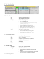
D F M
ata
rom
User Manual
by Cormac Purcell
31/10/2003
opra
Contents
1 Introduction – What is DFM?
2 The User Interface
2.1 The Load Panel
2.2 The Information Panel
2.3 The Scan Panel
2.4 The Message Panel
2.5 The Action Panel
2.6 The Save Panel
3. Reducing Position Switched Data
3.1 Preliminary Information - Register Usage
3.2 The Settings Dialog
3.3 Loading a Data File
3.4 Examining Data
3.5 Averaging Single Polarisation Data
3.6 Changing Polarisation
3.7 Averaging Dual Polarisation Data
3.8 Fitting a Baseline Polynomial
3.9 Zeroing Channels
3.10 Shifting the Velocity Scale
3.11 Saving Results
3.12 Quitting
1. Introduction- What is DFM?
DFM is a GUI interface to SPC, the spectral line reduction program used to process Mopra and
Parkes data. It is designed to enable the novice user to quickly and easily reduce dual-polarisation
position-switched data into a format usable by other programs such as CLASS and XS.
DFM contains the following features:
•
Automatically forms a quotent from signal and reference spectra on loading data.
•
Supports the following modes of position switching: ref-sig, sig-ref, ref-sig-sig-ref,
sig-ref-ref-sig.
•
Switches data to the LSR-K reference frame on load.
•
Allows seperate and independent reduction of both polarisation quadrants
•
Allows the user to inspect and flag bad scans in one click,
•
Aligns and averages scans in velocity space, weighted by (Integration Time)/Tsys2.
•
Correctly averages polarisation A and B together using correct header data.
•
Provides an interface fit polynomials to scan baselines with the option of accepting
or rejecting the results in a single click.
•
Allows the user to zero portions of the any scan.
•
Allows the user to shift the velocity scale on any scan based on the desired zero
velocity frequency.
•
Supports input of both .rpf and .sdf format data
•
Supports output in .sdf, .fits and .ps formats.
•
Corrects for the “Parkes Scaling Error” automatically for data prior to 05/09/02.
All of the above tasks may be performed manualy on the command line using spc, however this
would be a long and involved process. DFM automatically compensates for quirks in SPC that
might result in errors in the reduced data, should the user not be aware of them and take the
appropriate steps.
2. The User Interface
2.1 The Load Panel
Dir
Directory containing input file
File
Input file name with extention
Settings
Displays the settings menu.
Load
•
Type of file being read.
•
Accumulate individual integrations from a single
position? (rpf files only).
•
Correct for the Parkes Scaling Error?
•
Form a quotient from Signal – Reference?
•
Order of the scans in the file (Ref, Sig.....)
Load the file into the registry,
•
Switches to the LSR-K reference frame.
•
Form the quotients and plot the 1st scan
2.2 The Information Panel
Src
Source Name of the current scan.
Date
Date of observation
Freq
Frequency of Polarisation A (1st Quadrant).
BW
Bandwidth of Polarisation A
RA
RA in J2000
DEC
Dec in J2000
2.3 The Scan Panel
Green Box
Long Box
2.4 The Message Panel
Current scan / register displayed
Selectable list of scans
•
Select or de-select individual scans to average
together.
•
Clicked scans will be displayed and the values in the
Information Panel will update accordingly.
Blue Box
2.5 The Action Panel
Pol A / B
Sel & Average
Messages and feedback
•
Error and confirmation messages.
•
Tsys and Integration Time for the current scan.
Toggles between Polarisation A and B
Aligns and averages the selected scans in the current
polarisation.
Saves the result and remembers the scans selected.
Av A & B
Averages the results from “Sel & Average” on Pol A and
Pol B (Only available if Pol A and Pol B have been
averaged)
Fit Baseline
Displays the Fit Baseline Dialog
•
Zero Channels
Displays the Zero Channels Dialog
•
Shift Vel
2.6 The Save Panel
Dir
Fit a polynomial to the baseline (order 1-5).
Zero a selected range of channels.
Displays the Shift Velocity Dialog
•
Calculates a velocity shift based on a difference in
zero velocity frequency and a user specified frequency.
•
Velocity shift can be specified manually.
Directory to write out to.
File
File name prefix
File Type
Choose format of output file (.sdf, .fits, .ps)
Save
Save a the currently displayed scan using a the options
specified above.
Quit
End the program and save the settings last used.
3. Reducing Position Switched Data
3.1 Preliminary Information - Register Usage
SPC has a maximum of 256 registers which may be used to store scans. DFM reserves six registers
for its own use meaning that files containing more than 250 individual positions (Sig or Ref) will
need to be split.
In an individual scan Pol A data is stored in Quadrant 1, while Pol B data is stored in Quadrant 2.
If a data file contains n scans corresponding to n individual positions then the 6 registers
immediately after the nth scan will be used in the reduction process. The usage is allcoated as so:
Register
Usage
N
Last scan in the data set.
N+1
Average of selected Pol A scans (Quad 1)
N+2
Average of selected Pol B scans (Quad 2)
N+3
Average of Pol A & B scans (Quad 1)
N+4
Copy of Pol B scans copied to Quad 1(Save)
N+5
Temporary (Scratch) Register
N+6
Copy of Pol B scans copied to Quad 1(Av A&B)
3.2 The Settings Dialog
Before loading a data file it is necessary to tailor the file loading options to the data. Click on the
Settings button to display the settings dialog.
Choose the file-type, both sdfits and rpfits are supported.
Depending on the schedule file used during the observations adjacent scans may need to be
accumulated together. This will be the case if the telscope dumped data to the file more than once
per pointing. Choose Auto if you want to accumulate the individual integrations or straight
otherwise. Note- this option is only available when loading raw RPFits files.
Data taken before 5th September 2002 is affected by a scaling error introduced in the Telescope
Control Software. The amplitude of the Pol A data was multiplied by 1.51 and Pol B by 1.73 before
being written to the file. Selecting the TCS Scaling Error Correction checkbutton implements a
routine that removes these scaling factors from each scan based on the date of observation. If you
are loading previously corrected data from an sdf file you should turn this option off.
You can choose to form quotient scans from the reference and signal positions at load time. Four
observation schemes are supported at the present time:
1. Reference – Signal
2. Signal – Reference
3. Reference – Signal – Signal – Reference
4. Signal – Reference – Reference – Signal
These settings will be retained in a text file called .dfm_settings in your home directory and read
each time the program is started.
When finished click OK to dismiss the Settings Dialog and save the settings.
3.3 Loading a Data File
After configuring the load settings as above, type in the full directory path to your data directory in
the field labeled Dir. It is necessary to enter the last “/” in the path eg: /home/crp/data/
Type in the full file name, including extention in the field labeled File and click the Load button.
The data file will be read and loaded into memory using the options specified in the Settings dialog.
On load the following tasks are performed:
Accumulate (optional): RPFits files only. Concatenate all adjacent scans beloging to a
single position.
Rvel: Switch all scans to the LSR-K reference frame.
Scale Err (optional): If the observations were taken before 05/09/2002 correct the
amplitude of all the scans for the Parkes Scaling Error.
Quotient (optional): Form the quotient based on the observing scheme specified in the
settings dialog. The algorithm used is Q = (Tref.S)/R -Tsig where Tref and Tsig are the
system temperatures of the reference and signal spectra. Q, S, R are the quotient signal
and reference spectra.
A list of the scan numbers loaded appears in the Scan Selection Panel and the first scan is displayed
in the PGPLOT window.
3.4 Examining Data
The scan selection panel contains a list of all scans loaded into memory in the current polarisation.
Clicking on a scan number causes it to be displayed in the PGPLOT window and selects it for
averaging (highlighted in colour). Clicking a highlighted scan dedelects it.
The green box contains the number of the currently displayed scan.
3.5 Averaging Single Polarisation Data
Data from a single polarisation may be averaged together by clicking the Sel & Average button.
Highlighted scans are aligned in velocity space and then averaged together, weighted by (Int Time) /
Tsys2. The result is stored in reserved register and plotted for inspection. The selections made may
be specific to a single polarisation and both the result and the scans selected for averaging are
remembered by DFM.
3.6 Changing Polarisation
You may toggle between polarisation at any time by clicking on the button labeled Pol A / Pol B. If
you have already averaged scans from one polarisation the result will be displayed upon returning to
that polarisation, additionally the individual scans selected for averaging will be retained.
3.7 Averaging Dual Polarisation Data
Dual polarisation data may be combined by first averaging data from each polarisation individually
and then combining the two results. When both Pol A and Pol B data has been averaged (using the
Sel & Av button) the Av A & B button will become active. Clicking this button averages the Pol A
and Pol B data together weighted by (Int Time) / Tsys2. The resultant scan is stored in quadrant 1
(Pol A) of a reserved register and plotted for inspection.
3.8 Fitting a Baseline Polynomial
A polynomial of order 1-5 may be fitted to the currently displayed scan. Click on the Fit Baseline
button to display the Baseline Fitting Dialog. The x-axis of the plotted spectrum will change from
velocity to channel number. The baseline is fitted using two “baseline boxes” - regions of the
spectrum absent of any spectral lines. Choose two baseline boxes from the plot and enter in their
channel ranges in the fields provided, eg: 1075-1375 and 1698-1998. Be wary of syntax mistakes
here as SPC will return rubish results if you enter a text character by mistake. Choose the order of
polynomial to fit (1-5) from the menu at the top of the dialog box.
Click on Fit to see the effect of your chosen fit. If you wish to try again with new settings simply
click Revert to return to the original scan. When you are happy with the fit click Apply, changes will
be saved to the scan and the dialog box will close. Cancel aborts any changes made and exits from
the dialog box.
3.9 Zeroing Channels
Occasionally it may be necessary to set some chanels in an individual scan to zero, particiularly at
the edges of the bandpass. Click on the Zero Channels button to bring up the Zero Channels
Dialog. The x-axis of the plotted spectrum will change from velocity to channel number. Enter the
range of channels to be zeroed in the fields provided and click Zero to test. Revert returns to the
original scan. When you are happy with the result click Apply, changes will be saved to the scan and
the dialog box will close. Cancel aborts any changes made and exits from the dialog box.
Note: To achieve good results with this tool it may be necessary to fit a baseline to the scan in
quiestion first.
3.10 Shifting the Velocity Scale
When observing molecules with multiple transitions it may be necessary to shift the velocity scale
on the scans so that the zero position corresponds to a particular line. It is also possible that the
wrong frequency was centred in the bandpass due to errors while observing or otherwise.
Click on the Shift Velocity button to display the Offset Velocity Dialog. The current zero velocity
frequency is displayed (as requested at the telescope and uncorrected for VLSR of source). If this
frequency is different from the desired frequency simply enter in the desired zero velocity frequency
and click Calculate to compute the necessary velocity offset. The calculated offset will appear in the
Velocity Offset field. Alternatively the desired offset may be entered manually. The Test button
shifts the scale by the desired amount, Revert returns to the last scan. Apply causes the changes to
be saved to the scan and exits the dialog box. Cancel aborts any changes made and exits the dialog
box.
3.10 Saving Results
The currently displayed scan (indicated by the green box) may be saved at any time simply by
clicking on the Save File button. In the field labeled Dir enter the full path to the directory you wish
to write files to. You must include the trailing “/” as in the load panel. The File field contains the
prefix of the file to be saved, by default this is the source name as read from the input file.
Select your desired file type from the File Type menu. Supported types are SD-Fits and Fits and
Postscript plots. Click on Save Files to write the file.
Note: it is not possible to overwrite files of the same name.
3.11 Quitting
To exit the program click the Quit button. The choices made in the Settings dialog will be saved to
a text file named .dfm_settings in your home directory. DFM will read this file on the next startup.