Download User Manual for Australis

© Photometrix, Australia
www.photometrix.com.au
Version 7, October 2007
User Manual for Australis
Contents
1. Australis User Interface
Page
Page
5
2. Project Set up
2.1 Importing Project Images
2.2 Selecting the Camera
6
6
7
3. Automatic Measurement Operation
3.1 Procedure
3.2 Initial Camera Self-Calibration
3.3 Automatic 3D Measurement
3.4 Bundle Adjustment
3.5 Coordinate List and Point Dialog
3.6 Point Re-labelling
7
7
8
9
11
13
14
4. Setting the Scale
4.1 Automatic Scaling via Coded Targets
4.2 Scaling with Known Distances
4.3 Entering Scalebar Lengths into the Scale Database
17
17
17
20
5. Assigning the XYZ Coordinate System
5.1 Automatic Assignment of XYZ Axes
5.2 Operator Controlled 3-2-1 Process
21
21
21
6. Transforming to a Coordinate System via Control Points
6.1 Coordinate transformation
6.2 What is Needed for Coordinate Transformation?
6.3 Transformation Procedure
6.4 Point Re-Labelling via Coordinate Transformation
23
23
23
24
27
7. Quality Assessment and Results Summary
28
8. Exporting XYZ Coordinate Data
30
9. Automatic Camera Calibration
31
10. Lines and Colour
33
11. Point Referencing for Manual Measurement
11.1 Marking and Referencing
11.2 Undoing the Last Point Reference
11.3 Target Centroiding
35
35
38
38
12. Review Mode
39
13. Camera Selection and Camera Data Entry
13.1 Three Camera Scenarios
13.2 Unique Camera Identifier
13.3 Changing Cameras
13.4 Camera Databases
13.5 Listing the Global Camera Database
41
41
44
45
45
46
14. Generation of 3D Polylines
14.1 Polyline types
14.2 Polyline Creation
14.3 Selecting, Deleting and Colouring Polylines
46
46
47
49
2
14.4
14.5
14.6
14.7
14.8
14.9
14.10
14.11
14.12
Polyline Information Dialog
Polyline Length
Closed Polylines
Facet Versus Free-Form Polylines
Ambiguous Polyline Solutions
Planar and Non-Planar Polylines
Smoothed and Non-Smoothed Polylines
Referencing and Unreferencing Polylines
Summary of Hotkeys/Short Cuts
page
49
50
50
50
52
52
54
54
55
15. Texture Mapping To Generate Photo-Realistic 3D Models
15.1 Overview
15.2 Selecting Texture Mapping Mode
15.3 Planar Surface Entity Creation
15.4 Texturing
15.5 Generation of Constructed Points
15.6 Re-Texturing
15.7 Deleting Entities
15.8 Export of Texture Mapped Object in VTML format
15.9 Saving and Re-Loading the Project File
15.10 Summary of Hot-Keys
55
55
56
56
57
58
59
60
60
61
61
16. Adjustment of Image Scanning Parameters
16.1 Autoscanning
16.2 Autoscanning Control Dialog and Parameters
16.3 Target Scanning Parameters
16.4 Measurement Tolerance Parameters
16.5 Default Settings
16.6 Saving Autoscanning Settings
16.7 When to adjust the scanning settings
61
61
62
62
63
65
65
65
Appendix A Summary of Hotkey and Program Control Functions
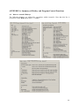
A1. Index to XYZ Hotkeys
A2.
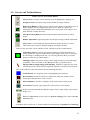
Cursors and Toolbar Buttons
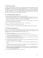
A3. Rotating an Image
A4.
Zooming within the Image View
A5.
Panning in the Image View
A6.
3D View Functions
A7.
Menu from Right-Click in 3D View
A8.
Menu from Right-Click in Image View
A9.
Deleting Images from the Project
A10. De-activating a Referenced Image
A11. Re-orienting an Image
A12. Re-orienting all Images
A13. Relative Orientation
A14. Re-linking a Folder of Images to a Project
66
66
67
68
68
68
68
69
69
69
70
70
70
70
70
3
A15.
A16.
A17.
A18.
Driveback
Single Image Resection
Entering a Point Description
Exporting Orientation Parameters and Image Coordinates
Appendix B The End-User License Agreement for Australis
page
71
71
74
74
75
Quick Reference Note
For a quick reference to all program controls such as toolbar buttons, cursors,
menus within the Image View and 3D View workspaces, refer to Appendix A.
Note on Camera Settings and Operation
Recall that there are three basic rules which apply to recording images for
photogrammetric measurement with Australis:
1. The camera lens should not be refocused during the photography session.
2. If using a zoom lens, the zoom setting should not be adjusted during the
photography session.
3. Where the camera has an ‘auto rotate’ function, which digitally rotates
the recorded image, turn this feature OFF.
4
1.
Australis User Interface
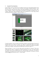
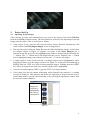
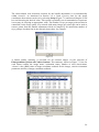
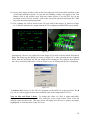
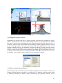
Upon running Australis (double-click on desktop icon) the user is presented with the screen
shown in Figure 1.1. There are two basic windows, the scrollable ‘Thumbnail Window’ at the
left of the screen which lists the camera(s) and image thumbnails used in the project, and a
main ‘Workspace’ window in which image measurement and graphics operations occur. An
example, which shows image thumbnails along with a graphical view of the image stations
and measured 3D point locations, is shown in Figure 1.2.
Figure 1.1
Figure 1.2
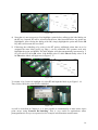
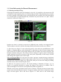
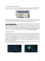
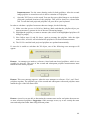
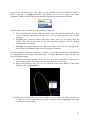
Generally speaking, Australis will be used to make automatic 3D measurements of an array of
targetted points on an object of interest. The targets for measurement points will usually
comprise retro-reflective ‘dots’ and coded targets will be employed to facilitate the automatic
measurement. Samples of dot targets and coded targets are shown in Figure 1.3.
Shown in Figures 1.1 and 1.2 are the main menus and toolbars for Australis. These have
deliberately been kept to a minimum to facilitate maximum ease of use. The menu options
and toolbar icons will be explained later and a full description of functions is provided in
Appendix A. Note that the list of Hotkey functions listed in Appendix A can also be accessed
from the Help pull-down menu or the ‘?’ on the toolbar.
5
Figure 1.3
2.
Project Set Up
2.1 Importing Project Images
Upon running Australis and commencing a new project, the operator first selects File|New
from the main File pull-down menu. The first function to perform is the importing of selected
images into the project. This is carried out as follows:
•
If the project is new, Australis will enter the Import Images function. Alternatively, this
can be selected with File|Import Images for an existing project.
•
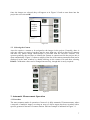
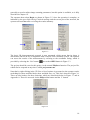
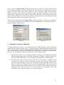
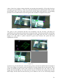
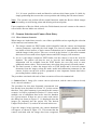
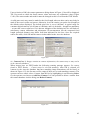
The user then selects from the Image Browser the folder holding the images. At this point
the window shown in Figure 2.1 appears. An image in the Select Image(s) list is
transferred into the project by first highlighting the image or images and then selecting the
‘>’ button. The ‘>>’ button moves all images into the project. Similarly, the ‘<’ button
moves highlighted images out of the project list, and ‘<<’ removes all images.
•
A single image at a time can be selected, or multiple images can be highlighted by either
dragging the mouse over the images (as shown in Figure 2.1; left-mouse click and drag) or
holding down the CTRL key while selecting multiple images. Holding down the SHIFT
key means all images between the two selected images will be highlighted.
•
Australis currently supports JPEG (*.jpg) and TIFF (*.tif) image formats.
•
If the image files do not contain information which identifies the camera(s), a warning
message is displayed. This indicates that before the importing of images into the project,
camera data must be entered either manually, or by selecting the appropriate camera from
the Australis camera database.
Images are
selected by
highlighting
the chosen
‘thumbnails’
Figure 2.1
6
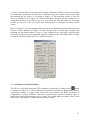
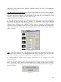
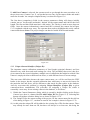
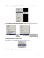
Once the images are selected, they will appear as in Figure 2.2 and to enter them into the
project the user selects OK.
Images
selected
for the
project
Figure 2.2
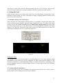
2.2 Selecting the Camera
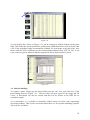
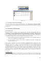
Australis requires a camera to be assigned to the images in the project. Generally, there is
only one camera per project, but there may be more than one. An up-to-date list of cameras
and their key metric design characteristics is provided with the Australis software. The
operator generally does not have to identify the camera or cameras used in the project; this is
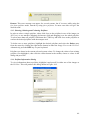
done automatically. Figure 2.3 shows a sample of the list of the camera parameters that can be
displayed in the main window by double-clicking on the camera icon and then selecting
Details. Calibration values can be changed interactively, though this is rarely required.
Figure 2.3
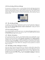
3. Automatic Measurement Operation
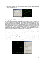
3.1 Procedure
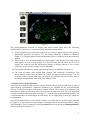
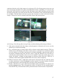
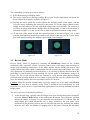
The most common mode of operation of Australis is fully automatic 3D measurement, where
a network of multiple images covering an array of object targets has been recorded with a
specific geometric network of camera stations. Such an example is indicated in Figure 3.1.
7
Figure 3.1
The photogrammetric network of images and object points must have the following
characteristics if Australis is to perform a fully automatic measurement:
i) Every targetted object point must appear in two or more images that provide good ray
intersection geometry (see Figure 3.1). The targets should be as distinct as shown in
Figure 1.3 (ie bright against a dark background such as is achieved with retroreflective
targets)
ii) There needs to be a sufficient number of coded targets, such that any five coded targets
must appear on two or more images. It is not necessary that all codes are seen in all
images, but codes provide the link between images so having subsets of five or more
codes seen in two or more images is quite important.
iii) The network should have strong convergent geometry, as indicated in Figure 3.1.
iv) The array of images must include both ‘portrait’ and ‘landscape’ orientations. This
means that the camera must be rotated or ‘rolled’ 90 degrees between images. It is not
necessary to have exactly half with a 90 degree roll and half with no roll, but some of
the images and preferably more than 30% must be rolled.
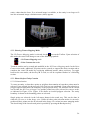
3.2 Initial Camera Self-Calibration
Automatic measurement with Australis requires that the camera be first calibrated, at least so
approximately representative calibration parameters are available for the auto-referencing
process, in which the camera calibration is further refined. This camera self-calibration step
generally need only be carried out once, the first time the camera is used. The self-calibration
uses the normal measurement network, Figure 3.1, with the only provision being that there are
a sufficient number of coded targets in each image. Six to eight codes or more per image are
recommended.
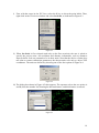
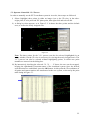
Once these requirements are met and the images are loaded into the project (stage indicated
by Figure 2.2), the network of coded targets is automatically measured to provide the camera
self-calibration. This is initiated by choosing AutoCal from the pull-down Photogrammetry
menu as indicated in Figure 3.2.
8
Figure 3.2
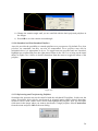
The initial self-calibration process concludes with a listing of the updated camera parameters,
as shown in Figure 3.3. A further more comprehensive account of automatic camera
calibration is provided in Section 9 of this Users Manual.
Figure 3.3
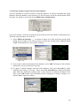
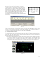
3.3 Automatic 3D Measurement
Once the initial self-calibraton has been completed (only if necessary), fully automatic 3D
measurement of the object targets can be commenced by selecting Auto-reference from the
pull-down Photogrammetry menu, or from the R++ toolbar button, as indicated in Figure 3.4.
Figure 3.4
Note on image scanning: Automatic measurement requires that all image points are detected
within the imagery in an initial image scanning process. This requires high contrast between
target blobs and background as well as particular characteristics for the image points. There is
9
generally no need to adjust image scanning parameters, but this option is available, as is fully
described in Chapter 16.
The operator then selects Begin, as shown in Figure 3.5. Once the operation is complete, as
indicated by the Auto Referencing Finished message and the screen plot of the network, the
operator selects Close after reviewing the results summary.
Figure 3.5
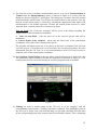
The basic 3D photogrammetric network is now measured, which means that its shape is
determined, but not its size or alignment with a chosen XYZ coordinate system. The operator
can assess the results of the measurement by referring to the coordinate listing, which is
provided by selecting the ‘List’ button
next to the OPEN button in Figure 3.3.
The project should be saved at this point, via the normal File|Save function. The project file,
which can be reopened at any time is called projectname.aus.
Note that by right-clicking in the 3D View a list of options is presented so the operator can do
such things as show and hide labels, show and hide axes, etc. This list is shown in Figure 3.6.
There are also hotkeys for these functions, which are listed both below in Figure 3.7 and in
Appendix A. These are accessed via the Help toolbar button and the ‘?’ button.
Figure 3.6
10
Figure 3.7
3.4 Bundle Adjustment
The final stage of the automatic measurement process within Australis is the bundle
adjustment, a least-squares estimation process that computes the photogrammetric network
orientation and thus the XYZ coordinates of all object feature points. There are a number of
circumstances that will lead the user to require a recomputation of the bundle adjustment at
the end of an automeasure sequence. This is initiated via the B toolbar button or the
Photogrammetry|Bundle menu selection, the associated dialog being as shown in Figure 3.8.
11
Figure 3.8
Upon selecting Run, the user will be presented with the statistics of the bundle adjustment
solution, namely the number of cameras employed, the number of image stations accepted
and rejected, the number of object points accepted and rejected. A number of important
metrics are also provided; these include the number of iterations involved, the image
coordinate misclosure value (RMS (microns)), the assigned minimum number of rays per
point, the observation rejection limit and the number of rejected image coordinate
observations. The numbers of single points, coded targets and code ‘nuggets’ are also listed.
It is often desired to re-run the bundle adjustment with altered tolerance values, the two most
common being the Minimum number of rays per point and the Rejection limit. The Setup
button is used to assign the new values, the dialog being shown in Figure 3.9.
Figure 3.9
12
A ‘fixed’ rejection limit (in micrometres) for image coordinate residuals can be set by ticking
Fixed and then entering the desired value, 5 microns in this case, which is much looser than
the automatically set value of 1.95 shown in Figure 3.8. The minimum number of rays has
also been changed to 3 in Figure 3.8, which means that a 3D point will be accepted if it is
triangulated by three non-rejected rays. It is very rarely the case that either the maximum
number of iterations or the convergent limit would need to be changed from their default
values.
Shown in Figure 3.10 is the summary dialog for the re-run bundle adjustment with the altered
tolerance values displayed in Figure 3.9. The relaxing of the rejection limit, coupled with
changing the minimum number of rays to 3, has resulted in two previously rejected points
now being accepted, but the adjustment quality is slightly poorer, the RMS value of image
coordinate residuals rising from 0.57 to 0.64 micrometres.
Figure 3.10
3.5 Coordinate List and Point Dialog
The 3D List of currently measured XYZ coordinates is obtained by clicking on the
button,
as indicated in Figure 3.11. The list shows the point labels (numbers or alphanumeric labels),
coordinates, number of images upon which the point appears, the RMS misclosure of
triangulation (a quality indicator, expressed in micrometres) and the maximum angle of
intersection between intersecting rays to a point. The overall RMS misclosure value is also
shown, as are the number of points and codes in the network.
13
Figure 3.11
A Point Dialog Box, shown in Figure 3.12, can be selected by double-clicking on the point
label. This shows the current point label, quality factor (RMS misclosure value in pixels), and
a list of the individual image measurement residuals for each image seeing the point. Also
shown with the XYZ coordinates are the corresponding standard errors (SX, SY, SZ). A red
cross, instead of green, indicates that the image point observation has been rejected.
Figure 3.12
3.6 Point Re-labelling
To re-label a point, simply type the desired label into the enter new point label box of the
Point Dialog shown in Figure 3.12. The new label will now appear in the Image and 3D
Views. A description can also be entered and this will be written to the DXF file on
coordinate output.
As an alternative, it is possible to manually relabel strings of points with sequentially
increasing numbers. This is more convenient when there is a lot of point relabelling required.
The steps are as follows:
14
1) Assume that it is desired change the labels of the points below in Figure 3.13 as follows:
27 to Edge_31, and then 25, 24, 23 and 21 to Edge_32 to Edge_35. Also, label 19 is to be
changed to Corner10. The changes can now be made in either the Image or 3D Views.
Figure 3.13
2) Select point 21 & then hit the F7 key. The following dialog, Figure 3.14, will appear
Figure 3.14
3) Enter the prefix ‘Edge_’ and use the arrow keys to select the start number, in this case 31,
as indicated in Figure 3.15.
Figure 3.15
Select OK and the point label will change to the desired new label, as in Figure 3.16.
15
Figure 3.16
4) Note that it is not necessary to first highlight a point before calling up the label dialog via
the F7 key. Instead, F7 can be selected and the new label inserted before any points are
highlighted. After closing the dialog with OK, simply highlight the point and hit the F8
key and it will assume the new label.
5) Following the relabelling of a point via the F7 option, additional points that are to be
assigned the same label prefix (eg Edge_) can be relabelled. The operator need only
highlight the point and hit F8. The label number will then automatically increment by 1.
So, you select 25 & hit F8, select 24 & hit F8, select 23 & hit F8 and finally select 21 &
hit F8 and the labels will appear as in Figure 3.17.
Figure 3.17
To rename 19 to Corner10, highlight 19, select F7 and input the label as per Figure 3.18.
Then, Select OK & the point will be relabelled.
Figure 3.18
As will be described in Chapter 6, it is also possible to automatically re-label entire object
point arrays using Network Re-Labelling. This is very useful in applications where
photogrammetric surveys are repeated, as for example in deformation measurement.
16
The next two steps in the Australis data processing sequence are to scale the object to true
scale and assign a particular Cartesian coordinate reference system to the object points.
4. Setting the Scale
There are three means to set object space scale, first via coded targets, second using a Scale
Database of stored scale bar values, and third by simply assigning distances between point
pairs in the object point array.
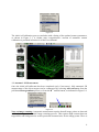
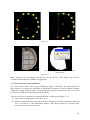
4.1 Automatic Scaling via Coded Targets
Since Australis uses coded targets of known sizes, it is possible to assign object space scale
based on point-to-point distances between points forming the codes. To achieve this initial
scaling, the user ticks Scale via codes from the Edit|Project Settings menu and ensures that
the correct coded target size is also ticked (there are three standard size options). The dialog
appears as in Figure 4.1. Selection of this option causes red scaled distances to be shown for
coded targets within the 3D View, as shown in Figure 4.2.
Figure 4.1
Figure 4.2
Cautionary Note:
The distances used to scale the network via coded targets are very short and thus small
uncertainties in the mean scale will be magnified for larger point-to-point distances in the
network. It is therefore recommended that scaling via codes be used where a preliminary scale
of only moderate accuracy is required. Higher accuracy scaling requires one of the following
two approaches.
4.2 Scaling with Known Distances
To set a true scale to the XYZ coordinates, the operator must specify one or more point-topoint distances. The scaling process proceeds as follows:
17
i) First, with the cursor in the 3D View, select the L key to show the point labels. Then,
right-click in the 3D viewer window and select Set Scale, as indicated in Figure 4.3.
Figure 4.3
ii) When Set Scale is first selected (and only on the first occasion), the user is asked to
specify the project units. All coordinate and distance information, such as distances
input to define scale are assumed to be in these units. Note that the choice of units does
not relate to camera calibration parameters; the chosen units refer only to object XYZ
coordinates. The units are defined by choosing one of the four options in Figure 4.4.
Figure 4.4
iii) The dialog box shown in Figure 4.5 then appears. The operator selects the two points A
and B (from the number list) forming the known distance, and this distance is entered.
Figure 4.5
18
iv) To register the scaled distance, click Apply. At this point, or later, you can add
additional distances for scale control, or even change or delete previously entered
distances. Once all data is entered, press Close. Red lines will be drawn between the
pairs of nominated ‘scale points’ in the Image and 3D Views. The final scale will be a
weighted average of the nominated scaled distances. Figure 4.6 indicates a scale
distance in the 3D View. The S key can be used to toggle the red line between show and
hide in both the 3D and individual Image Views.
Figure 4.6
v) As an alternative to entering the numbers for points A and B, as in (iv), first
highlight/select two points. Left-click in either the 3D View or Image View (with the
Select tool) and then CTRL/left-click for the second point. Then, select Set Scale. The
two selected points will be shown as Points A and B and the operator need only enter
the distance and press Apply followed by Close. This is shown in Figure 4.7.
Figure 4.7
In order to check point-to-point distances after scaling, simply highlight the two end points of
a line in the 3D view, right-click and then select Distance from the menu.
Cautionary Notes:
a) In the event of a drastic rescaling of the network, the 3D view may look too small or large
and may require rescaling via either the mouse wheel or the Increase or Decrease view scale
options (see Figure 3.6). The camera size may also need rescaling (the ‘1’ and ‘2’ keys).
b) Unless Set Scale is employed to fix one or more point-to-point distances, the object
coordinates will be at an arbitrary scale (ie objects will not be at true size). A warning is given
in this case to set scale if coordinates are to be exported via DXF or a text file, or if the project
is closed without first establishing a scale.
19
4.3 Entering Scalebar Lengths into the Scale Database
Australis maintains a Scalebar Database of known distances. In order to automatically assign
distances from the database to the network, it is first necessary to tick the option shown below
in Figure 4.8, which is accessed from the Edit|Project Settings menu.
Figure 4.8
Users who employ a scalebar on many projects need only enter the distance information once.
This data entry procedure is as follows:
i) Select Edit/Scale database … , as shown in Figure 4.9a. This will bring up the Scale
dialog shown in Figure 4.9b. The next step is to enter the scalebar name, endpoint labels,
length and standard error (enter 0.001 if unsure).
Figure 4.9a
Figure 4.9b
ii) To store the scalebar information in the database, select Add. The input of such scalebar
information can be performed at any time.
iii) To apply a scalebar distance from the scale database, first select Set Scale by rightclicking in the Image or 3D view. Then, select Get from DB and a dialog will appear
from which the particular scalebar name can be selected, as indicated in Figure 4.10.
Then, select OK and the scale information will be displayed as shown in Figure 4.11.
Select Close to apply the scaling.
Figure 4.10
20
iv) To remove a scalebar entry from the database, simply select the Delete button in the
dialog shown in Figure 4.11.
Figure 4.11
5. Assigning the XYZ Coordinate System
The process of photogrammetric orientation can be carried out within an arbitrary XYZ
Cartesian coordinate system. In Australis, this coordinate system has its origin at the first of
the relatively oriented images, and its XY plane is aligned with the focal plane of the camera
at that station. In most cases the user will wish to assign a more useful XYZ reference system.
This assignment of the coordinate system origin and orientation is carried out via the so-called
3-2-1 process. First, a point is selected to define the origin (X,Y,Z values of zero). Next, a
point through which the X axis will pass is defined, and finally a third point is selected to
define the XY plane and therefore the direction of the Z coordinate axis.
This process can be carried out either automatically via coded targets, or manually by
selecting appropriate object points an then choosing the 3-2-1 command. These two XYZ
datum assignment options will now be described.
5.1 Automatic Assignment of XYZ Axes
Open the Edit|Project Settings Dialog and enter the desired labels for the origin point, Xaxis point and the point to define the XY plane orientation, as indicated in Figure 5.1. This
choice of XYZ coordinate system can be made at any time, but it will only come into effect
with the running of a bundle adjustment. Thus, select the B toolbar button if necessary. The
resulting coordinate axes are displayed in the 3D View, as shown in Figure 5.1.
Figure 5.1
21
5.2 Operator Controlled 3-2-1 Process
In order to manually set the XYZ coordinate system in Australis, these steps are followed:
i) Select (highlight) three points in either an image view or the 3D view, in the order:
origin point, X-axis point and XY-plane point, then right-click and select 3-2-1.
ii) A dialog box then appears, as in Figure 5.2. It shows the three points and the default
axes, as well as the newly assigned axes.
Figure 5.2
Note: The three points for the 3-2-1 process can also be selected (highlighted) in an
image window, but the 3D view is necessary for viewing the newly assigned axes. The
3-2-1 process can also be selected without highlighting points, in which case point
numbers are entered via the dialog box.
iii) By interactively checking the selected +X, -X, ... , -Z boxes, the axes can be swapped,
keeping the right-handed Cartesian nature of the coordinate system. Once the desired
axial directions are established, press the OK button. At this point the 3D coordinates of
all points and camera stations are transformed to the new system, as shown by the point
table listing in Figure 5.3.
Figure 5.3
22
6. Transforming to a Coordinate System via Control Points
6.1 Coordinate Transformation
There are many situations where it is desired to tie the photogrammetrically measured 3D
point coordinates into an existing coordinate system, which is defined by ‘control points’.
Control points have known coordinates in two Cartesian reference systems: they have Xc, Yc,
Zc coordinates from the existing Primary or ‘control’ coordinate system, as well as X, Y, Z
coordinates from the specified Secondary or Australis 3D reference system.
In such instances, it is usually desired to transform all Secondary coordinates into the Primary
or control point system. Australis accommodates three coordinate transformation options, a
block shift, 2D transformation within the XY plane, and a full shape-preserving 3D similarity
transformation. The 3D transformation will be of most use to Australis users and so it will be
explained in more detail here.
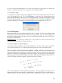
3D transformation: Given three or more control points that are non co-linear, a 3D
transformation can be performed from the specified Secondary XYZ system to the Primary
XcYcZc system of the control points. The transformation involves a translation, three rotations
and possibly a uniform scale change. This represents the general transformation case, and 2D
transformations and block shifts are special cases of this general case. Figure 6.1 illustrates a
2D coordinate transformation. Basically, the provision of control points allows transformation
into any chosen object space Cartesian (XcYcZc) reference system.
6.2 What is Needed for Coordinate Transformation?
In order to transform Australis XYZ coordinates into another reference coordinate system,
control points are required (either a text file of control point coordinates or interactively input
coordinate values). A sample control points file is shown in Figure 6.2.
a) Control points in
Primary Xc,Yc system
b) Measured points in
Secondary X,Y System
c) Measured points transformed
into the Primary Xc,Yc system
Figure 6.1: 2D transformation of XY coordinates (Secondary system) into Xc,Yc coordinates (Primary system)
via four control points (Points 2, 10, 11 and 15).
Control Points File. The format for each point record in the file must be: Control Point label,
Xc, Yc, Zc. Not all points need also be measured in the Australis project, though clearly the
minimum number of common point is three non co-linear points for a 3D transformation. If
more points are used a least-squares estimation process is adopted to obtain a best-fit solution.
Also, the point labels of the control points file and the Australis points do not need to
correspond exactly.
23
Interactive Entry of Control Points for Coordinate
Transformation. It is also possible to enter the control
points interactively, directly into the listing within the
dialog box shown in Figure 6.3. Select the New Point
button. Each time this button is selected a new control
point record will appear, with XYZ coordinate values of
N/A and with a label of NEWPOINTi, where i is
incremented. This dialog will be further explained in the
next section.
X
C-15 595.3
C-21 1383.6
C-33 1381.2
C-40 178.9
C-44 184.5
Y
743.6
1246.7
0.0
5.1
1253.0
Z
30.4
-0.9
-0.0
41.2
43.5
Figure 6.2
Figure 6.3
Once the desired number of control point entries is entered, simply highlight the cell in which
a value is to be entered and insert the correct label/coordinate value, as shown in Figure 6.3.
To remove a control point, right-click on the label and select Remove.
6.3 Transformation Procedure
The following procedure can be performed at any time after the 3D points measurements have
been made, and after ensuring that the desired control points have also been referenced and
therefore measured in 3D by Australis.
i) Because the transformation to control points process involves a point ‘linking’ operation,
it is useful to initially have the 3D View open in the Workspace, with the point labels
turned on (the L key). It might also be useful to have an image open for better visual
interpretation of the control point layout. An example 3D View is shown in Figure 6.4.
Figure 6.4
24
ii) The first step in the coordinate transformation process is to select Transformation to
Control from the Photogrammetry menu, as shown in Figure 6.4. At this point the
dialog box shown in Figure 6.3 will appear. This dialog has a window where the control
point coordinates will be listed. Two actions are required here by the operator: First, the
desired transformation must be selected by clicking the appropriate radio button (3D
transformation is the default selection). Second, the control points need to be either
imported from a control points file or interactively input.
Note on Scale: One of the two messages will be given in the dialog regarding the
adopted scale of the transformed coordinates:
a) Scale Set and Held - scale has been set in the Australis project and will be
maintained.
b) Control Points Scale Adopted - means that the final scale of the transformed
coordinates will be that of the control points system.
The program will adopt option (a) or (b) purely on the basis of whether scale has been
set in the project. If scale has been set in Australis, the user must first delete the scale
information from the 3D View (ie no red scaled distances in the 3D View) in order to
adopt the scale of the control point coordinates.
iii) Select Import Control Points in the case where control points are to be read from a file.
The point labels and coordinates will then be displayed, as indicated in Figure 6.5. The
control points text file can be built using an accessory program such as NotePad.
Figure 6.5
iv) Linking. In order to match points in the 3D view or in the image(s) with the
corresponding control points, a ‘linking’ procedure is adopted. First, highlight a point in
the 3D View or image view (left-click and drag over the point) and then click the label
of the corresponding point in the control points list (left hand column). This is illustrated
25
for 3D Points 21, 33, 40 and 44 (Control: C-21, C-33, C-40 and C-44) in Figure 6.6.
Note that once the control point has been referenced, a green tick mark will appear. Also
the label in the 3D view and images will change to that of the control point. If the point
is the first to be linked, the coordinate origin will move to that point. Continue this
process, ensuring that at least the minimum number of points for the desired
transformation have been linked: 1 for a block shift, 2 for a 2D transformation, and 3 for
a 3D transformation. A warning message will be displayed if a linked control point label
is the same as an existing referenced point. The already referenced point will then have a
‘1’ appended to its label.
Figure 6.6
Note: When moving the cursor from the control point dialog box to the 3D View or the
image view, the window for these two views may not become active until a cursor
action is initiated. To activate the windows, simply left-click within the window.
v) Linking via the List of Reference Points. A second method to link control points to
referenced points is to right-click on the control point label and select Link to … The
desired point is then selected from the list of referenced points by left-clicking on the
label in the referenced points list and choosing OK. This is illustrated in Figure 6.7.
Figure 6.7
vi) The Transformation Computation will occur automatically, as soon as enough control
points are referenced to their corresponding measured points. Upon transformation, the
coordinate axes in the 3D View will move to correspond with the Control Point
Reference System, as shown in Figures 6.6 to 6.8. At this time, ‘transformation
residuals’ will be displayed in the columns headed DX, DY and DZ in the control points
dialog box. In the case of there being more control points referenced than necessary,
these coordinate discrepancy values can be used to indicate the quality of shape
26
correspondence between the measured and the control point networks. This is illustrated,
by the example shown in Figure 6.8 where 5 points have been linked for a 3D
transformation; the magnitude of the residuals indicates the level of shape/size
correspondence between the two networks. Non-zero residuals will always be apparent
for a 3-point 3D transformation. An overall quality value for the transformation, which
is only applicable for cases of more control points than necessary, is indicated by the
Quality: RMS = *.**, which is shown in Figure 6.8 with the value 0.025 mm.
Upon transformation to control, the position of all control points will be shown in the
3D view in blue. The blue labels for these can be toggled on and off with the N key.
Figure 6.8
vii) Linking Closest Points. As shown in Figure 6.8, after a transformation solution is
obtained a listing will be made of the referenced points which lie closest to the
‘unlinked’ control points. The distance discrepancies are indicated for the unlinked
points in the columns DX, DY, DZ and Total (vector distance). In most cases, if the
values are small & consistent with the DX,DY,DZ values for linked points, then there is
a good chance that the closest point is also the correct point to be linked to the
corresponding control point. To achieve an automatic linking of the closest points,
simply choose the Link Close Points button, which will be greyed out until an initial
transformation solution is obtained.
viii) Unlinking Control Points. In order to either unlink a control point, or remove the point
from the control listing altogether, right-click on the control point and make the required
selection. When a point is unlinked, a new point label is assigned to the corresponding
point in the 3D view. This will also occur if a linked control point is removed. It is
possible to unlink all points, but in doing so the XYZ coordinate system will remain in
its current position.
ix) The transformation process is now complete and the Close button can be selected. If at
any time following the transformation to control it is desired to again assign a new XYZ
coordinate system, this can be achieved via the standard 3-2-1 procedure (Section 5).
Similarly, scale can be re-set via the standard approach (Section 4).
6.4 Point Re-Labelling via Coordinate Transformation
There are many instances where object points are measured repeatedly, for example in
deformation monitoring surveys where it is desired to quantify point movement over time.
Because the automated referencing procedure assigns point labels automatically, the
27
numbering sequence for non-coded targets can change between repeat surveys. Australis
offers a feature whereby point labels from a previous survey can be assigned to a repeat
measurement through the coordinate transformation process. The procedure is basically
identical to that for the 3D coordinate transformation to ‘control’, except that when a point is
re-labelled it retains its original coordinates, i.e. there is no transformation of XYZ values.
To initiate the Re-labelling, select Point Re-labelling Only from the control points dialog
(see Figure 6.8) and proceed through steps (iii) and (iv) of the coordinate transformation
procedure i.e. import the control file & perform the linking, but with a relaxed Closeness
value. Once linked, the ‘control point’ labels will be assigned to the corresponding object
points.
Figure 6.9
7. Quality Assessment and Results Summary
Australis updates the photogrammetric orientation and object point coordinates through a
process called bundle triangulation every time a point is referenced. Thus, the final measured
3D data is always up-to-date and no special orientation processing step needs to be selected at
any time by the user. If required, however, the bundle triangulation can be performed, as
described in Section 3.4, by simply selecting the B button on the toolbar and then Run. This
produces a summary of the bundle adjustment listing the number of points and images as well
as other information, as shown in Figure 7.1. Clicking on the buttons labelled Camera(s),
Stations or Points will give listings for these parameters, as shown for example for the camera
stations in Figure 7.2.
Figure 7.1
28
The observational error detection criterion for the bundle adjustment is set automatically
within Australis. As mentioned in Section 3.4, a fixed rejection limit for the image
coordinates observations can be set by selecting Setup (Figure 7.1) and then ticking the Fixed
box and choosing the desired value. This option is generally not recommended as experience
is necessary in selecting an appropriate value. The number of rays per target point can also be
controlled via the Setup option. In a network with many images per point, this can be used to
remove points from the bundle adjustment which are imaged by an insufficient number of
rays, perhaps less than four in the network shown here, for example.
Figure 7.2
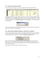
A further quality summary is provided for all oriented images via the selection of
Photogrammetry|Orient all Camera Stations. This summary, shown in Figure 7.3, lists for
each camera station the image name, orientation status, number of used observations,
‘closure’ value (RMS value of image coordinate residuals for the image), exterior orientation
parameters and list of image coordinate residuals.
Figure 7.3
29
Prior to exporting the measured 3D coordinates, it is desirable to assess the accuracy of the
overall photogrammetric survey. Information related to the quality of the full measurement
process is contained in the Summary, which is available through selecting the S button on the
toolbar. A sample summary is shown in Figure 7.4. This can be printed via the Print button.
Note the measurement accuracy summary in the figure. It states that scale has been set and
that the individual 1-sigma accuracies for the X, Y and Z coordinates are 0.024, 0.023 and
0.029mm, respectively. The relative accuracies are also listed, as is the internal accuracy of
the photogrammetric triangulation, which is here 0.07 pixels (1/15th of a pixel) suggesting a
0.6 micrometer accuracy for image coordinate measurements on the Nikon D100 images in
this project. It is important to verify the quality of the results before the XYZ object point
coordinate data is exported for further analysis.
Figure 7.4
8. Exporting XYZ Coordinate Data
The final XYZ coordinates can be exported for further analysis and for CAD modelling
purposes. There are two options, the first as a listing of XYZ coordinates and coordinate
standard errors (sigma X, sigma Y, sigma Z) in an ASCII text file (filename.txt), and the
second as a DXF-formatted file of XYZ coordinates (filename.dxf) which may include
attribute data (eg lines, point identifier numbers, colours). To export the coordinates, select
the XYZ coordinate list
(button next to OPEN above the camera icon) and then select
either of the Export … options.
30
Upon selection of Export DXF, the dialog box indicated in Figure 8.1 will be shown and the
user is asked to select the text size for the DXF file. Also, there are four options. The first is to
include a Network Label Prefix. The second is to write a ‘dummy’ origin point to the file,
which is simply a record with the point label ‘origin’ and XYZ coordinates of (0,0,0). The
third relates to whether the user wishes to output to the DXF file text descriptions entered for
points. The default option for Include descriptions is to output the text point descriptor strings.
The fourth option relates to the output of Offset Points.
There are also output options for Export TXT, as shown in Figure 8.2. These cover inclusion
of code points, the ordering of the output ASCII file in alphanumeric order and the inclusion
of the coordinate standard errors.
Figure 8.1
Figure 8.2
9. Automatic Camera Calibration
As briefly discussed in Section 3, the basic procedure for fully automatic camera calibration
within Australis follows closely that for a normal automatic photogrammetric measurement.
The only distinction is that the initial AutoCal procedure involves the use of coded targets
alone. The user needs an array of preferably 20-30 coded targets. To illustrate the process here,
however, we will simply use the same network as in the previous sections.
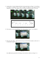
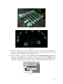
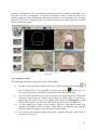
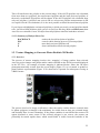
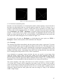
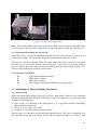
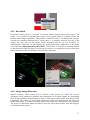
i) Establish the target array. Using the principles of having a well spread array which
fills the image format and is preferably non-planar, establish a suitable target array.
The array is shown in Figure 9.1. (Normally, more codes than 12 should be used).
ii) Determine the camera station geometry and record the images as JPEGS (at full
resolution). The primary items to remember are that a) the camera station network
provides strong convergence angles, b) The images are taken such that at least 3-4 of
them are ‘rolled’ (90˚ rotation), c) the codes are distinguishable with each code dot
being of high contrast and larger than 5 pixels in diameter in the imagery and d) it is
preferable if all codes do not lie in the same plane. The geometry of the ship
component survey, shown in Figure 9.2, is a good example.
31
Figure 9.1
Figure 9.2
iii) Load the images into a new Australis project in the normal way, as described in
Section 2. At this point the project camera will have been identified and the image
thumbnails will be displayed in the thumbnail window.
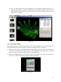
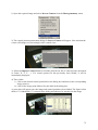
iv) Run the automatic calibration. Select AutoCal from the Photogrammetry menu as in
Figure 9.3. (same dialog box as in Figure 3.2). The operator then selects Begin and the
automatic calibration proceeds. Each image is sequentially processed and once the
calibration is complete the calibration results are displayed, as indicated in Figure 9.4.
Figures 9.3
32
v) Save the calibration data. Upon completion of the automatic calibration the user is
asked whether he/she wishes to update the local camera database with the new
calibration data. The normal response would be Yes. The project can then be saved and
the process is complete.
Figures 9.4
10. Lines and Colour
Lines joining points can be drawn in both the 3D View and Image Views. The procedure for
drawing lines, between just two points or between multiple points, is as follows:
i) Select the Line Cursor via the Line Button on the toolbar, the line cursor being a short line
with a cross at each end. The cursor ‘point’ is the dot adjacent to the upper cross. The line
cursor can also be selected in the image view using the L key.
ii) Click the Colour Button on the tool bar. This will generate the colour chart shown in
Figure 10.1. Click on the desired colour and then click OK.
Figure 10.1
33
iii) In any of the image windows click on the first end point of the desired line and then on the
second and subsequent points. To stop the line building, simply click again on the Line
Button, click in the window away from any feature points, or use the ESC key on the
keyboard. In the 3D view window, click on the first point and then hold down the CTRL
key when selecting subsequent points.
iv) The resulting line will be drawn in the 3D view and in the images, as shown in Figure
10.2, and line attributes are output with the XYZ coordinates with the DXF export option.
Figure 10.2
Alternatively, the user can right-click in the Image View while in Select Mode and choose
Line. This brings up the dialog box shown in Figure 10.3. After selecting the two endpoint
labels from the pull-down list, the line length will be displayed. The operator then chooses
the colour and selects OK (twice if a new colour is set), at which point the line is displayed.
Figure 10.3
To delete a line, Select it in the 3D View and then use the DEL key on the keyboard. The D
key can be used to toggle between show and hide lines in the Image and 3D Views.
Note on Line and Point Colour: To change the colour of a line or point (and label),
highlight the line or point in the 3D View and click on the colour button. Then, select the
desired colour and press OK. (The new colour will apply after the line or point is no-longer
highlighted; ie click anywhere in the 3D View)
34
11. Point Referencing for Manual Measurement
11.1 Marking and Referencing
Following the automatic network orientation in Australis, it is possible to also measure the 3D
coordinates of non-targetted points via a Referencing procedure. This manual process can also
be used to initially orient images where coded targets are not available, but in this description
it is assumed that an initial automatically measured 3D point network is in place. Such a
situation is indicated in Figure 11.1.
Figure 11.1
Imagine now that it is desired to measure an additional point, usually a non-targetted point.
The procedure to do this is called referencing. Briefly, the actions to take are as follows:
1) Enter Reference Mode: To enter referencing mode, select either the green R button on the
toolbar, or simply the R key on the keyboard. Or, when there are three or more images open,
click on the red ‘R’ button on the image titlebar of the two images you wish to reference; the
R button will then turn green. The cursor will now change to a green ‘pencil’. Referencing
simply entails the successive marking of the same point, sequentially in each image, with the
order being either right to left or left to right.
Note on Navigate Mode: If at any time you wish to ‘navigate’ around the images, hold down
the Space Bar on the keyboard and Navigate Mode will be selected. Left- and right-clicking in
navigate mode zooms the image view. Recall also, that you can move the image by holding
down the mouse wheel and moving the mouse.
2) Reference the point(s) of interest: The actual marking is illustrated in Figure 11.2. As
shown, it is generally desirable to enlarge the image of the point to be marked. This is
achieved through one of the four zoom options described in Appendix A.
With the pencil cursor positioned on the point of interest, click the left mouse button and a
purple cross will mark the desired point. A sequence number, which has no importance at this
stage, will also appear. This is the case in Figure 11.2. Then, move to the second image
35
where a blue line is shown, along which the correspond point should lie. (If the blue line does
not appear, press the B key). A line also joins the marked point (with the pink label) and the
green pencil. Now, go to the same point in the second image and mark the corresponding
position. The two label markers now turn green and a number is assigned to the point.
Figure 11.2
The point is now referenced and has 3D coordinates, but the accuracy will likely be
significantly lower than the measurement of targeted points. Upon the successful referencing,
the new point label (62 in this case) will appear in the Image and 3D Views, as shown in
Figure 11.3 (the label is yellow instead of green here because the point has been
highlighted/selected).
Figure 11.3
3) Referencing Predicted Points: After the new point is referenced (and therefore measured in
3D) in two images, its position can be predicted in all other images that see that point. These
points are labelled in blue (if the ‘blue’ points are not displayed, move the cursor over the
image and select the B key). So, if the user now chooses to reference the image point 62 in the
third image, he/she must first un-click the green R button of one of two referencing images
36
and then click the red R of the image to be referenced. The R will turn green (or the user can
turn referencing off and back on again via the R toolbar button or the R key). To reference the
blue point, first click close to point 62 in the left image (green label) and then precisely mark
the image point (don’t just click near the blue label; its position is only predicted and may not
be accurate). The blue label will turn to green and so point 62 is now referenced in three
images. This process can be continued with other images and desired points.
Figure 11.4
4) Deleting a Point During Referencing: Points are deleted during referencing as follows:
i) If the point selected in the first image (coloured purple) is deemed to be in error, use the
Delete key to cancel the marking.
ii) For a referenced pair of points (while still in reference mode) hold down the CTRL key
and the cursor will change to the Select cursor (arrow). A marquee box can then be drawn
over the points(s) to be either unreferenced or deleted altogether. Also the point label in
all images containing that point will turn yellow. Using the DELETE key will then unreference the points and they will revert to red ‘marked’ status only (hence they are no
longer 3D points). Clicking on these points in reference mode (after the CTRL key is
released) will turn them purple and DELETE will remove them completely.
iii) When in reference mode, a right-click on the mouse will present the user with the option
to either unreference or delete highlighted (yellow) points. For points already referenced
in other image pairs, unreferencing will occur only in the current image.
iv) Finally, if the 3D view is open, the left-mouse button can be pressed and a box drawn over
points to highlight them. They will again turn yellow, in both the 3D view and the images.
The DELETE key will unreference these points and remove them from the 3D points list.
37
11.2 Undoing the Last Point Referencing
It is possible to undo the most recent point referencing operation by selecting CTRL+Z or
choosing the pull-down menu selection Edit|Undo last referenced point: # (Figure 11.5).
Figure 11.5
In the case where a point is already referenced, this operation un-references the point pair and
deletes the new point marking. Through this function it is possible to undo referencing in the
reverse order to which is was carried out, stepping backwards through the points.
Note on displaying images: It is possible to have multiple images open at different
enlargements. It is thus often useful to return all images to full image view. To achieve this,
simply use the SHIFT + F keyboard combination. To return a single image to full view, use
the F key on the keyboard. Also, in order to close all images that are displayed, but not being
referenced, either select Window|Close NonReferencing or call up the Select Cursor (use
CTRL key when in reference mode), right-click and choose Close Non-Referencing Images.
Finally, to evenly tile uneven windows, simply select either Window|Tile or SHIFT+T.
11.3 Target Centroiding
The optimum targets for precise marking and referencing are likely to be high contrast dots.
Where such targets are utilised, Australis can fine-measure them during manual referencing
with an auto-assist function that provides precise centre-of-target (centroid) determination. In
order to perform an automatic precise marking in either Referencing or Single Image Point
Marking mode (Photogrammetry menu, red pencil cursor), the Centroiding function can be
employed. By selecting the X key for white blobs on a dark background, or the C key for
dark blobs on a light background. (Recall: select Referencing or Marking mode first, followed
by the centroiding function).
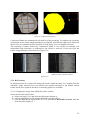
The centroid tool determines the precise centre (centre of gravity) of a target ‘blob’. In this
case the centre of target G in Figure 11.6 is required:
Figure 11.6
Figure 11.7
38
The centroiding operation proceeds as follows:
i) Select Referencing or Marking mode.
ii) The cursor is placed over the target and the X key (or C key for dark blobs) is selected; the
zoom window then appears as shown in Figure 11.7.
iii) Moving the mouse within the window adjusts the intensity profile of the target, with the
red cross always indicating the centroid (centre point). To see the image window clearly,
simply move the mouse to the top right-hand corner of the zoom window. The aim here is
to isolate an image blob which is distinct from its background, ie it has a closed border as
indicated in Figure 11.8, and its red cross is stable with small movements of the mouse.
iv) A left-click of the mouse records the centroid position, as shown in Figure 11.9. A final
centroid determination has thus been made to an accuracy that may well be 5 times better
than with manual marking for suitably exposed high contrast targets.
Figure 11.8
Figure 11.9
12. Review Mode
Review Mode, which is initiated by selecting the Edit/Review button on the Toolbar
(Indicated with a capital E), allows a point-by-point review of all image point markings (ie
image point referencing operations). As the name implies, Review Mode represents a final
quality control procedure which is commenced once the network has been formed. It is really
only appropriate for manually referenced points, so it will only be briefly described here. By
presenting a visual display of every marking for a given point, as indicated by point 13 in
Figure 12.1, the review process allows the operator to verify that the same physical feature
point has been precisely marked in every image. If this is not the case, the operator can either
move the marked point to the correct position or delete it if desired.
Caution: When the network contains many very large images (say 10 at >8mb each), Review
Mode can be very slow to initially set up. Thus, it should be used infrequently for such
networks, or even not at all. It is generally only appropriate for reviewing manually measured
image points.
The review process is carried out as follows:
i) At the desired stage, typically after all images have been oriented and points referenced,
select the Review Mode button on the toolbar (the E button). The workspace will then
display the images. In Figure 12.1, the manually referenced point 13 is shown. Note the
small dialog box which allows the user to move forward to the next point, move
backwards to the previous point or move to any selected point (by selecting the number
from the list). Also, the number of imaging rays to the point is shown, the maximum
39
intersection angle, and a Quality Value which is the RMS value of image measurement
errors (in pixels) for the individual triangulated point. Values in the range of 0.05 to 3.0
would be expected for this. Finally, there are zoom buttons to further enlarge or reduce
the images (all together).
Figure 12.1
Note on number of images displayed: In Review Mode, only six images will be displayed
at any one time. The operator can use the ‘>>’ or ‘<<’ buttons to move forward to the next
subset of nine image chips of the point currently being reviewed, or back to the previous
subset. Thus for a network with 36 images, the user must proceed, if desired, through six
subsets of six image sets to review all possible images.
ii) The marked, referenced point in any image can be dragged to a new position using the
blue pencil cursor and by holding down the left mouse button (if the blue predicted
points are not being displayed, hit the B key).
iii) Every time a point is ‘moved’ in Review Mode, the full network is immediately
recomputed, so small changes will be seen in the Point Table list, especially for the
point being reviewed.
iv) In instances where multiple points appear in an enlarged image view, only the current
point can be adjusted.
v) Where a point does not lie within the format of an image, a red cross will be shown in
the centre of the image.
vi) On the other hand, if the ray from an object point to a camera station does fall within the
image format then the predicted point location will be indicated in blue, as in Figure
40
12.1. It is now possible to mark and therefore reference this feature point, if visible, by
simply positioning the cursor at the correct position and clicking the left mouse button.
Note: The operator can perform all the normal functions within the Review Mode images
such as zooming, un-referencing points and deleting referenced points.
Upon completion of Review Mode (select the Finish button) Australis returns to the status it
was at before Review Mode was selected.
13. Camera Selection and Camera Data Entry
13.1 Three Camera Scenarios
When images are loaded into Australis, one of three possibilities arises regarding the selection
of the camera(s) and camera data:
i) The images contain an EXIF header which identifies both the camera and important
camera parameters, especially the focal length. The Australis camera database already
has details of this camera, so basic camera information can be immediately associated
with the images in the project. This case, covered in the Section 2, is the most common
that Australis users with newer digital cameras and JPEG imagery will encounter.
ii) As in (i), the images contain an EXIF header, but the camera is not in the Australis
database. The camera will then be new to Australis and although certain camera
information will be available from the EXIF header, the user may need to enter
additional camera values. This scenario may arise when using a newly released camera.
iii) The final scenario is where the images have no EXIF header and so Australis cannot
determine from the imagery alone the make, model and calibration parameters for the
camera. In this case the user will be prompted to enter important camera data before
proceeding further with the project.
The procedure associated with each of these scenarios will now be summarised.
i) Camera Case 1: Image files contain camera information, and the camera data is already
in the Australis database
The procedure for this most frequently encountered case
has already been described in Section 2.2. In this section,
therefore, only a brief summary is presented for this camera
scenario. As will be explained in Section 13.2, there can be
multiple sets of calibration data in the Australis database
for a given camera. If there are two or more such entries,
the dialog box shown in Figure 13.1 is displayed when the
images are imported into the project list. The desired
Unique ID (Section 13.2) needs to be selected in this case.
Upon the images being imported, the camera thumbnail
will appear, as shown in Figure 13.2. This means that the
camera associated with the images has been recognised,
Figure 13.1
41
and that it exists in the Australis database. Multiple cameras can also be accommodated
within the one project.
Note Regarding Image Resolution: It is highly recommended for accuracy reasons that the
digital camera be used at the ‘correct’ resolution setting. It is best not to use resolutions where
the image dimensions (in pixels) are either higher or lower than the pixel dimensions of the
camera. If the camera is 3008 x 2000 pixels, then use the
image resolution of 3008 x 2000.
A list of the camera parameters can be generated in the main window by double-clicking on
the camera icon, this list being shown in Figure 13.2. Calibration values can be changed
interactively, though this is only infrequently required for the case of a previously calibrated
camera already residing in the database. Caution must be exercised in altering camera
calibration values. If nothing is known of these, other than the approximate focal length value
which must always be entered, the values should be left at either their previously calibrated
values, or at zero.
Figure 13.2
Note: If the focal length in the EXIF Header is more than 1mm different from that for the
same camera in the database, a new Unique ID for the camera should be set at this time. This
will create a second set of calibration parameters, as explained in Section 13.2.
ii) Camera Case 2: Images contain camera information, but the camera is not in the
Australis database.
In the case where the images have EXIF header information about the camera, but the camera
data is not already in the Australis camera database, the warning message shown in Figure
13.3 is displayed to indicate that some camera data will need to be entered before the project
images are loaded.
Figure 13.3
42
Upon selection of OK, the camera parameters dialog shown in Figure 13.4a will be displayed.
The User needs to check the listed camera values and enter any calibration values (Figure
13.4b). The camera make and model cannot be changed as this is read from the EXIF header.
A valid (non-zero) entry must be made for the focal length, whereas other entries need only be
made if the correct values are known. Otherwise, leave the entries (except the focal length) at
the default values displayed. The default pixel size is set to 0.005mm. A typical range for
consumer digital cameras is 0.003mm to 0.009mm, and it is desirable – though not mandatory
– to enter the correct value here if it is known. Adoption of the default pixel size will lead to a
satisfactory camera calibration and subsequent 3D measurement, but the computed focal
length (principal distance) may differ from that indicated for the lens. Once the required
entries are made, click OK and the camera is then added to the Australis database.
Figure 13.4
iii) Camera Case 3: Images contain no camera information; the camera may or may not be
in the Australis database
When images have no EXIF header the following warning message appears: No camera
found in EXIF Header … Camera must be selected manually. After OK is selected, all
cameras in the Australis database that have matching image dimensions will be listed, as
shown in Figure 13.5 (the list may well be empty if there are no such matching cameras). The
operator can now either select a camera from the list by highlighting it and choosing Select.
Or, the operator can choose to Add New Camera. It is also possible to delete a camera from
the camera database via this dialog (use Delete Camera).
Figure 13.5
43
If Add New Camera is selected, the operator needs to go through the same procedure as in
the previous case (Camera Case 2), except that here an entry for the camera make and model
must also be made. An example completed entry is as shown in Figure 13.6.
The first three (compulsory) fields in the camera parameters dialog will always initially
contain ‘not set’ for the make and model, ‘default’ for the camera name and 0.00 for the focal
length. The first and third field must have valid entries. The Tab key is used to move between
fields. Once the camera information is entered and OK is selected, the camera list in Figure
13.5 is updated with the new entry. The operator then needs to highlight this newly entered
camera and choose Select. The project images can then be loaded in the normal manner.
Figure 13.6
13.2 Unique Camera Identifier (Unique ID)
The important camera calibration parameters of focal length (principal distance) and lens
distortion vary with focus and zoom settings for a lens. The possibility then arises, that for a
given camera in the Australis database, multiple sets of calibration data might be needed if the
camera is employed either at different lens focus, or with different lenses or zoom settings.
This can create difficulties because the same camera name, etc. will be read from the EXIF
header in the images, but the essential calibration data, which may or may not be known for
the particular lens and focus, will be different to that stored for that camera in the database.
Australis overcomes this problem by assigning Unique Identifiers (Unique IDs) to given
camera/lens/focus combinations. The procedure for assigning a Unique ID, which is
essentially a new entry for an existing camera in the database, is as follows:
i) Within the Camera Parameters dialog, which is opened by double-clicking on the Project
Camera icon, there is a button labelled Add Unique ID (See Figure 13.2). Selecting this
button will produce a further dialog box as shown in Figure 13.7a.
ii) The Unique ID for the camera setting of the project, for the camera named in the title bar
of the dialog in Figure 13.7, can then be entered. An example is shown in Figure 13.7b.
iii) At this point the unique ID will be added to the existing list of IDs for that camera. There
may already be more than one ID, but there will always be at least one, this being the
44
‘default’ ID. If a camera has only one set of calibration data recorded in the database, then
it does not need a Unique ID.
Subsequent selection of Add Unique ID will show all IDs listed (Figure 13.7c). The dialog
will now also show the Unique ID and the parameters related to that camera setting.
(a)
(b)
Figure13.7
(c)
13.3 Changing Cameras
The user may wish to change the camera (and camera parameters) associated with the project
images (either a single image or a group of images). For example, it may be desired to change
from the default camera to a calibration set associated with a particular Unique ID. There are
two ways to change the project camera:
i) The most common procedure will entail double-clicking on the Project Camera icon and
then selecting the Change Camera button in the Camera Parameters dialog box (see
Figure 13.2). This will open a list of cameras, from which the desired camera/Unique ID
combination can be selected. After clicking on the desired camera, select the Change
button. Note that only cameras with the correct image dimensions will be displayed.
ii) A second way to invoke the Change Camera function is to right-click on one of the
image thumbnails. The procedure is then the same as in (i), except that in this case only
the image concerned will be assigned the new camera.
13.4 Camera Databases
Australis utilises two camera database files: a read-only ‘global’ database and a ‘local’
database. All cameras utilised in projects will be entered into the local database. Thus,
whenever Australis searches for a camera, it first looks in the local database, after which it
accesses the global database. The distinction between the two is not apparent to the user. The
global database is ‘read-only’ so that no editing of this is allowed. On the other hand, cameras
can be added or deleted from the local database, as required, through normal Australis
operations. Descriptions have been given as to how to add a camera to a project, and hence to
the local database, and how to delete a camera from the local database via the Change Camera
option. To delete a camera from the camera database, select Edit|Camera Database|Local, as
indicated in Figure 13.10. This then brings up the dialog box shown in Figure 13.11, which
lists all cameras in the local database. To delete a camera from the list, and therefore
permanently from the local database (but not the global database), highlight the camera and
select Delete.
45
Figure 13.10
Figure 13.11
13.5 Listing the Global Camera Database
To list all cameras in the Global Camera Database, select Edit|Camera Database|Global.
The user can then scroll through the list of cameras, but cameras cannot be added to or deleted
from this list.
14. Generation of 3D Polylines
14.1 Polyline types
Previous versions of Australis have supported only 3D point determination from the
referencing of corresponding image points in overlapping images. Sometimes, edge detail and
curved features are found where point referencing is difficult or not feasible. In such cases it
is now possible to determine 3D Polylines, which do not require the specific referencing of
corresponding image points. Australis can generate two types of polylines:
i) Facet polylines, which are best suited to geometric figures whose boundary points (eg
corners) are recognisable in multiple images.
ii) Free-form polylines, which are best suited to defining curved lines, a straight edge
being the simplest case.
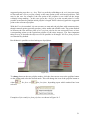
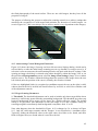
Two examples of polylines are shown (in selected or highlighted mode) in Figure 14.1. The
arch above the door is a 3D free-form polyline generated from non-corresponding point
markings, whereas the rectangle at the top of the door is a facet polyline that has
corresponding corner points, but note that these are not referenced points. The arch could also
have been generated via the facet polyline method. Both polylines in Figure 14.1 were
referenced via the two right-hand images, with their positions in the lower left image being
from back-projection (equivalent to blue, predicted points). Their 3D location is shown via
the 3D View.
Cautionary Note
The generation of polylines is an inherently less accurate and often less robust procedure than
the creation of single 3D points through referencing. Indeed, there are many possible image
46
geometry configurations where the polyline determination will be subject to systematic error,
and may even fail. Consequently, care needs to be taken to ensure a) that the project will
produce accurate polyline information, and b) that polylines free of systematic error are being
generated. This can be checked in part via visual assessment of the back-projected polylines
in non-referencing images.
Figure 14.1
14.2 Polyline Creation
The following procedure is adopted to create a 3D polyline:
i)
In order to draw polylines, switch to the Polyline Marking Mode by selecting
on the toolbar. This is only possible in Referencing Mode
. Either Facet or
Free-form polylines are available, as mentioned above and detailed later.
ii)
You can create a polyline now in one of the two referencing images by clicking the
left mouse button along the desired object. Select as many points as necessary to
approximate the object. If you are not happy with a point, press backspace to undo
the last clicked point. To cancel the whole drawing process, press the ESC key.
iii)
To stop adding more points to the polyline, click the right mouse button. The
polyline will change colour to purple, which advises you that any new polyline
drawn on the other images will be referenced to this polyline.
iv)
Go to the second referenced image and create a polyline along the same object as
described in ii) and iii).
47
Important note: Use the same drawing order for both polylines. After the second
image polyline is created Australis is able to calculate a 3D polyline.
v)
Open the 3D View to see the result. You can also open a third image to see the backprojected (predicted location of the) polyline. This will be shown as a dotted blue
line. To turn the back projected polylines off, press N on your keyboard.
In order to calculate a polyline from more than two images, do the following:
1) Make sure that you are in PolyLine Marking Mode and that the polyline object you
want to measure is present in one of the two referencing images.
2) Highlight the polyline you want to measure (the colour of the highlighted polyline will
change to purple).
3) Now follow steps ii) and iii) above, again to measure the polyline. After the right
mouse click, Australis will recalculate the polyline in 3D from all measurements.
4) The 3D View and the back projected polylines are updated automatically.
If Australis is unable to calculate the 3D object, one of the following error messages will
appear:
Reason: An attempt was made to reference closed and non-closed polylines, which is not
possible in Australis. The type of the second and subsequent polyline measurements must
match the first drawn polyline.
Reason: This error-message appears, when the user attempts to reference ‘Free’ and ‘Facet’
polylines together. The polyline type of the second and subsequent referenced polylines must
match the type of the first drawn line!
Reason: Australis was not able to determine the common start and/or end points between two
or more referenced polylines. Suggestion: if this message occurs, try to use exactly the same
start and end points rather than using different points.
48
Reason: This error message can appear for several reasons, but if it occurs while using the
free-form polyline mode, instead try using facet polylines. In most cases this will give the
desired result.
14.3 Selecting, Deleting and Colouring Polylines
In order to select a single polyline, either click close to the polyline in one of the images (or
3D View), or use marquee dragging (left-mouse click and dragging) over the whole polyline.
To select more than one polyline, hold down the CTRL key and click close to the polylines or
enclose the desired polylines with the marquee tool.
To delete one or more polylines, highlight the desired polylines and select the Delete entry
from the menu by clicking the right mouse button in either the Image View or the 3D View.
Alternatively press the DEL key on your keyboard.
Polylines are drawn in the current selected system colour. To change the colour of an existing
polyline, first highlight it, then click the colour button in the toolbar, choose a colour in the
dialog and press OK.
14.4 Polyline Information Dialog
To view information about a polyline, highlight it and press P in either one of the images or
the 3D View. This will produce the dialog shown in Figure 14.2.
Figure 14.2
49
In order to change the default label, or to add a description for the polyline just change the
entries new polyline label and/or text string description and press OK.
14.5 Polyline Length
To determine the length of a polyline, highlight it and click the right mouse button in either
one of the images or the 3D View. Select Distance… from the menu. Depending upon the
units used and whether or not the scale is set, a dialog similar to that below will appear, listing
the length of the polyline. If more than one polyline is selected only the length of the first
polyline is displayed. The length of a selected polyline is also displayed in the 3D View.
14.6 Closed Polylines
Both closed and open (non-closed) polylines can be created. To close the polyline being
working on, move the mouse pointer to the first clicked polyline point. A small rectangle over
this point will then appear. Just press the left or right mouse button and Australis will close
the polyline automatically.
Important note: As previously mentioned, it is not possible to mix closed and non-closed
polylines in the calculation of a single 3D object.
14.7 Facet Versus Free-Form Polylines
Australis provides two different ways to draw polylines – the Facet and Free-form methods.
The preferred method is Facet as this usually leads to more accurate and reliable results.
The facet polyline method provides the capability to define polylines using discrete points
(such as distinctive corners, edges, pixel brightness variations, etc) where it is possible to see
common points between images. Of course this restricts the choice of points as the polyline
needs to be defined by corresponding points in the images. The polyline can start and end on
different points, as illustrated in Figure 14.3 below. Notice that the resultant 3D polyline will
consist of only the common segments measured between the images.
Figure 14.3
Since common points are selected with Facet polylines, Australis suggests the next point to be
measured on the referenced polyline. Additionally, a guiding line is shown in the image in
which the polyline is currently being marked, as shown in Figure 14.4. To change to the next
50
suggested point press the + or – key. This is a perfectly valid thing to do, as it is not necessary
to start and end a Facet polyline exactly at the same points as the referenced polylines. This
may be the case for example if the first point of the polyline is not visible on the image
currently being marking – in this case, press the + key to go to the second point. It is also
possible to measure beyond the initial polyline’s length. If this is desired, ignore the suggested
point on the referenced polyline.
With the Free-form method, it is not necessary to start and end polylines with common points,
though common points generally produce a more stable and reliable result. The points marked
in between the first and last point of a Free-form polyline do not necessarily have to have
corresponding points on the equivalent polyline in the other image(s). The most important
thing is to try to describe the object as well as possible in all images. All Free-form polylines
are smoothed by default.
Recall that it is possible to close both types of polylines.
Guiding line
Next referenced
polyline point
Current
measured
polyline
Figure 14.4
To change between the two polyline modes, click the down arrow next to the polyline button
on the toolbar and select the desired mode. This will change the icon of the polyline button to
either
selected.
for facet or
for free-form, depending upon which method has been
Examples of facet and free-form polylines are shown in Figure 14.5.
51
‘Facet’ polyline
Back projected polyline
‘Freeform’ polyline
Figure 14.5
14.8 Ambiguous Polyline Solutions
Sometimes the operator will have to mark a polyline where the blue guiding line closely
follows the path of the actual object feature being measured. For example, the blue guiding
line may be parallel and overlapping the white road paint that defines the edge of a lane. In
such cases Australis may have problems in determining a unique solution, and this is caused
by the overall geometry of the camera station network. The dialog below, which lists all
possible solutions Australis can determine, will then be shown. To help select the correct
solution it is useful to open the 3D View as well as a few additional images in which the
polyline is back projected. The selected solution in the dialog will be shown in the open views
so that the correct solution can be visually determined. Once OK is selected, there is no way
to change it, so care must be taken to ensure the correct solution is chosen.
14.9 Planar and Non-Planar Polylines
Quite often the object featured being measuring using polylines in the images are planar, for
example building facades, road surfaces, car panels, etc. A planarity constraint can be added
to ensure the polyline lies within a plane. Alternatively, the planarity constraint can be
52
removed for non-planar cases. This option is only available in PolyLine Marking Mode or
when a polyline is highlighted/selected. The default selection is to impose the planar
constraint, with the choose being made through the pull-down menu from the toolbar:
There are three ways to add/remove the planarity constraint:
1. When activating the PolyLine Marking Mode, choose the polyline method (Free-form
or Facet) and the constraint in advance. Every newly created polyline will use these
settings.
2. Highlight one or more polylines and select either planar or non-planar from the
toolbar. The 3D object(s) and all the back projected polylines will be changed
immediately to reflect this.
3. Highlight one polyline and press the right mouse button in the 3D View to bring up the
menu; then select Planar to add/ remove the planar constraint.
Once the planarity constraint is added to a polyline, it is possible to adjust the adopted plane
by changing the rotation angle and rotation axis. To change the rotation angle and axis, use
the following procedure:
i) Zoom to the desired polyline in the 3D View. It is also a good idea to open one or
more image(s) where the back projection of this polyline can be seen.
ii) Select one polyline in the 3D View and click the right mouse button. In the menu
displayed, select Adjust Plane.
iii) Notice the red line below; this is the rotation axis. Use either the default rotation axis
or adjust the axis by unselecting Use default rotating axis and changing the line points
considered for the rotation.
53
iv) Change the rotation angle until you are satisfied with the back projected polylines in
the images.
v) Press OK to save the rotation axis and angle.
14.10 Smoothed and Non-Smoothed Polylines
Australis provides the possibility to smooth polylines as a post process. By default Free-form
polylines are smoothed, but they can also be unsmoothed. Facet polylines may also be
smoothed where it is appropriate to do so. To toggle between smoothed and non-smoothed,
highlight one polyline and press the right mouse button in the 3D View to bring up the menu
shown in Figure 14.6. Select or deselect Smoothed from the menu to toggle the status of the
polyline.
Figure 14.6
14.11 Referencing and Unreferencing Polylines
Sometimes the operator may not be satisfied with the calculated 3D polyline. In this case the
entire 3D polyline object can be unreferenced in selected images and/or deleted altogether.
Switch to Select mode (white arrow cursor) and highlight the polyline. Now use the rightclick menu in the image where you want to unreference a single polyline. Select Unreference
from the menu and press OK on the next dialog.
54
This will unreference the polyline in the current image. If the old 3D polyline was calculated
from more than two polylines, the unreferenced polyline and the back projected polyline of
the newly recalculated 3D polyline will be shown. If the old 3D polyline was calculated from
only two polylines, it will now not exist in 3D (as at least two polyline measurements in 2D
are required for the 3D calculation). It is also now possible to delete the unreferenced polyline.
If you forgot to highlight the referenced polyline to which your newly created polyline should
refer, just select both polylines while you are in PolyLine Marking Mode and Reference them.
Australis now calculates a new 3D object from all polylines related to both those selected.
14.12 Summary of Hotkeys/Short Cuts
BACKSPACE
ESC
N
P
undoes the last clicked point of polyline
cancels whole drawing process of current polyline
turns back projected polylines off
shows information about selected polyline
15. Texture Mapping to Generate Photo-Realistic 3D Models
15.1 Overview
The process of texture mapping involves the ‘mapping’ of image patches from selected
Australis project images onto planar surface entities defined on the 3D object model displayed
in the 3D View. An example of texture mapping is indicated below, where the 3D object
photogram-metrically created from the seven images (Figure 15.1a) is textured to produce a
photo-realistic representation (Figure 15.1b) that can be exported for subsequent viewing in
VRML format.
Figure 15.1a.
The process involved is image rectification, where the surface entities that are textured must
be planar polygons (a triangle is the minimum), be visible from at least one oriented image
and desirably have a convex boundary. If the planar condition is not fulfilled the texture will
appear distorted to some extent. If the selected polygon is not convex, the texture can
potentially be turned upside down, which would make it visible from the backside of the
55
entity, rather than the front. If no oriented image is available, or the entity is too large to fit
into one orientated image a default texture (white) appears.
Figure 15.1b.
15.2 Selecting Texture Mapping Mode
The 3D Texture Mapping mode is selected via the
icon on the Toolbar. Upon selection of
this mode, the cursor will change to one of the following symbols:
= 3D Texture Mapping mode
= Point Construction mode
Textured entities can be created and modified in the 3D Texture Mapping mode. In the Point
Construction mode, additional 3D points can be created, to support the entity creation and to
complete the visual 3D model by overlaying additional texture where necessary. To toggle
between the two modes, the hot key W is used, as will be explained further in a following
section.
15.3 Planar Surface Entity Creation
15.3.1 Point selection
To create an entity, at least three points or polylines that contains at least three points must be
selected. Lines created via the Australis Line Tool are not considered. Upon point selection, a
polygon appears that shows the boundary of the proposed entity. The selection can be carried
out in either the 3D View or Image View and the points have to be selected in a convex order,
as indicated in Figure 15.2a. Figure 15.2b shows an invalid polygon selection. The entity
boundary is drawn as the bounding points are selected.
Single points are selected via the left mouse button in the usual way. This can be done in
either the 3D view or in the Image view. Unlike all other point selection modes in Australis,
predicted (blue) points can also be selected in the Image View when in texture mapping mode.
The deselecting of the last selected point is possible by pressing the Backspace key.
56
(a) correct selection
(b) invalid selection
Figure 15.2. Selected boundaries for entity creation
15.3.2 Selection of polyline points
Polylines can form boundaries of textured planar surface entities and they can be selected in
the same way that single points are selected, again in either the 3D View or Image view. A
polyline is internally stored as a sequence of 3D points and it is possible to use only a subset
of these in the texture mapping process. To ‘shorten’ a polyline from each end for texturing,
use the Backspace and CTRL + Backspace to deselect points from both sides/ends of the
polyline. To aid in this process, points of the polyline are highlighted and the start and end
points are coloured green and red. For a closed polyline, at the beginning the start (green) and
end (red) are the same and appear in red, as shown in Figure 15.3.
To deselect the red point use Backspace to deselecting the green point use CTRL +
Backspace. Further selected points will be attached to the end point.
15.4 Texturing
The texturing step follows immediately after the planar surface entity is generated. To texture
a selected, bounded entity press the right mouse button in the 3D View. The image patch to be
rectified onto the surface entity will be automatically selected based on the geometry of the
images forming the network. Normally, the best image is that whose orientation in 3D is most
parallel to the entity surface. Only images from side of the viewing direction, from which the
user is looking at the entity in the 3D View, will be considered.
As an alternative to automatic texture selection, the user can specify a given image from
which the texture will be taken. In this case, which occurs quite frequently because the
automatic selection might not be the optimal choice because of occlusions or image quality,
the user simply clicks the right mouse button within the desired Image view, or he/she selects
(highlights) a chosen thumbnail within the thumbnail view and presses the E key.
The texture mapping of the entity will result in one of three outcomes, as shown in Figure
15.4. In the first, a texture will be mapped to the surface in the 3D View. In the second, a
yellow fill will appear, along with a message that there is no texture available (eg the selected
entity is being viewed from the backside in the 3D View). In the third, a default texture is
assigned to indicate that the entity spans more than one image (ie entity is not contained
within a single image).
57
Selected points of a polyline
Polyline with four points excluded
Figure 15.3.
Textured entity
Warning message, if no texture is available; blank
default texture
Figure 15.4.
Note: Textures can be toggled off and on via the Z key, and entities can also be
created/textured when the visibility is toggled off.
15.5 Generation of Constructed Points
3D ‘Constructed Points’ can be created within the plane of an entity. The main purpose of
these points is to enable the definition of additional sub-entities to allow further texturing
within an existing textured entity. Constructed points appear in red in the 3D View. Point
Construction mode is invoked by pressing the W key.
There are two ways to generate a Constructed Point, as indicated in Figure 15.5:
a) Click on an existing entity in the 3D View, or
b) Select an entity first (this represents a plane in 3D space) and click somewhere in the 3D
View or ImageView. The intersection point of this chosen image ray and the plane
results into a constructed 3D point.
58
(a) Point construction within an entity
(b) Point construction in relation to an entity
Figure 15.5. 3D point construction
Constructed Points are automatically selected for a later texturing. To complete the texturing,
switch back to the texture mapping mode by pressing W, and click the right mouse button (in
the 3D View for automatic texture selection or in the Image View for manual selection).
The texturing of entities formed by Constructed Points is very useful for texturing over
obstructions and occlusions, as indicated by the effective ‘removal’ of the pole from the
texture mapped façade section shown in Figure 15.6.
Texture mapped pole to be removed
Pole is cut out; Constructed Points used to define an
additional entity, which is textured
Figure 15.6.
15.6 Re-Texturing
In situations where it is required to change the texture within an entity, for example when the
automatic image selection does not produce the optimal texturing or the default (white)
texture needs to be replaced, the three re-texturing options are available:
15.6.1 Changing the image from which the texture is taken
Select the relevant entities, then:
a) choose an Image View and click the right mouse button, or
b) select a thumbnail of in the thumbnail window and press E, or
c) click the right mouse button in the 3D View, and choose Recalculate Texture from the
menu shown in Figure 15.7.
59
15.6.2 Assigning an artificial texture
It is possible to assign an artificial texture to a planar entity. This is often required when the
default texture (no orientated image is available for texturing) appears. Select an entity and
click the right mouse button and the Entity menu (Figure 15.7) appears. With Set Texture, an
artificial texture (8bit, or 24bit TIFF, or JPG file) could be chosen. The texture will be
stretched onto the chosen entity.
Through use of the Point Construction mode and artificial texturing, unrecorded areas of the
3D scene can be texture mapped in this way. This is a particularly useful way to fill small
gaps between complex textured entities.
Figure 15.7. Menu resulting from right-click in a selected entity within the 3D View.
15.6.3 Mapping the entity on its reverse side
It is possible to texture map an entity ‘from behind’, ie to have the texture visible from the
opposite direction. To achieve this, first select the entity in the 3D View and then rotate it into
the position where the texture should be visible. Now, either:
a) choose an Image View and click the right mouse button, or
b) select a thumbnail of in the thumbnail window and press E, or
c) click the right mouse button in the 3D View, and choose Recalculate Texture from the
menu shown in Figure 15.7.
Note: To make the entity visible from both sides, a second entity must be created. See: “How
to create an entity?”
15.7 Deleting Entities
To delete an entity or entities, select the entities and press the Delete key. Sometimes
overlapping objects of the OpenGL View and Image View are simultaneously selected. You
can choose individually which group of objects have to be deleted.
15.8 Export of Texture Mapped Object in VTML format
The virtual reality modelling language (VRML) is a well known 3D data format. The textured
entities including the 3D vertices, image points of the texture and the texture itself can be
exported using the Entity menu (Figure 15.7). A sample VRML view is shown in Figure 15.8.
In addition to the VRML file, textures are saved as JPEG files. The image files comprise
rectified images of the entities. A VRML Viewer is required to view the exported model.
60
VRML model
Boundaries of entities
Figure 15.8. Views of the VRML model
Note: The textured entities will not be exported into DXF format, but the Constructed Points
will be exported. Only geometric elements are stored in the exported DXF file from Australis.
15.9 Saving and Re-Loading the Project File
When the project is saved an additional subfolder for the entity textures is created in the
current project folder. The subfolder contains the rectified entity images as tiff files.
If the project is moved to another folder, the image path of the entities has to be set in much
the same way as occurs with normal Australis projects. In this case, to re-link the textures,
select an entity, right click, and choose Select Image Path in the Entity Menu (Figure 15.7).
The new image path can be assigned for all entities.
15.10 Summary of Hot-Keys
W
Z
D
E
toggle point construction mode
toggle entity visibility
toggle line visibility
for texturing with selected thumbnail of the project Bar
16. Adjustment of Image Scanning Parameters
16.1 Autoscanning
Within the autoscanning process, the aim is to detect ‘white blobs’ which are well contrasted
against a dark background. Whether each of these blobs is a valid target or not depends upon
a number of blob properties:
a) How ‘white’ it is compared to the background, ie is its greyvalue intensity sufficiently
higher than the background?
b) Its size, ie is it too big or too small?
c) Its shape, ie is it elliptical and not long and thin?
Note in Figure 16.1 that there are four detected potential targets. The code is recognized, as is
the valid target at the left of the figure, but the other two detected blobs are ‘hot spots’ from
61
the flash photography of the metal surface. These are not valid targets, but they have all the
properties of targets.
The purpose of allowing the operator to adjust the scanning controls is to achieve settings that
maximize the recognition of valid targets and minimize the detection of invalid targets. As
seen in Figure 16.1, this is not always easy to achieve and it is very dependent on the imagery.
valid target
invalid targets
Figure 16.1
16.2 Autoscanning Control Dialog and Parameters
Figure 16.2 shows the Image Scanning and Auto-Measurement Settings dialog, which can be
selected before or after the initial image scanning process (eg after R++ or imagescan only). If
selection is after an autoscan, the autoscanning must be run again with the new settings. After
opening an image, the dialog is selected using either the Q key within the Image View or via
the pull-down Photogrammetry menu selection Image Scan Settings (Image View window
must be active). The window within the dialog shows the portion of the image where the user
left-clicked (note the position of the cursor). Initially, this window is blank.
Of the two highlighted blobs (ie recognized as candidate targets) the one on the right is valid,
whereas that on the left is invalid, but classified here by Australis as valid. Now consider each
of the adjustment controls.
16.3 Target Scanning Parameters
1) Threshold: The threshold adjustment can be used to include only those target blobs whose
intensity is sufficiently greater than the surrounding background. The threshold greyvalue step
between background and a target will be larger for a highly reflective target. The default
setting is 20 greyvalues (the maximum for an 8-bit image is 255) and a suitable setting for
retrotargets against a moderately dark background is anywhere from 15 to 50.
Note what happens when the threshold in Figure 16.2 is changed to 36, as shown in Figure
16.3. Only the valid target remains and the ‘hotspot’ is not classified as a candidate target.
Typically, sliding the threshold value to the right causes less blobs to be found, and more
blobs (ie higher noise) are found when it is moved to the left.
62
invalid target
valid target
Figure 16.2
Figure 16.3
2) The Maximum Width (or diameter) simply specifies the largest size that a blob may have
to be classed as a valid target. The default size is 50. There is no adjustable minimum size,
that width being about 4 pixels. The ideal sizes for target blobs are from 5 to 30 pixels.
3) The width-to-height or ‘W/H’ ratio is one measure of blob shape. A value of 1 would
normally indicate a near-circular blob, which is generally what is required. A value of more
than 4 (the default) would indicate a very thin, elongated blob, which is likely invalid.
16.4 Measurement Tolerance Parameters
The next four parameter values that can now be interactively changed relate to the point
measurement process and specifically to the determination of matching unlabelled image
points. These parameters are Rank Value, Intersection Angle, Minimum Number of Rays
and Driveback Tolerance. The function of these individual adjustments is as follows:
63
1) The Rank Value expresses the geometric tolerance applying to the ray-intersection
geometry during the determination of corresponding non-coded targets in multiple images.
There is a range of values from 1 to 5, with three being the default. Basically, the smaller the
value, the larger the number of possible point matches (true targets and erroneous hot-spot
targets). Thus, although more possible matches will be made, the automeasure process will
slow down as this value is decreased towards 1. The admission of possibly many more
erroneous point matches is not such a problem because these will usually be edited out in the
final bundle adjustment. The recommended action here is to start with the default setting of 3.
If valid target points are missed, then reduce the value to 2 and select R++ and CONTINUE
to re-run the Automeasure (it is not necessary to re-scan the images). Reduce the value to 1 if
true target points are still missed.
2) The Intersection Angle Limit is an important tolerance to apply since it is often the case
in networks with many images that erroneous targets arising from such factors as sun
reflections are seen in closely adjacent images, which often means that they have very small
angles of intersection. This is depicted in Figure 16.4, where the point out in the right side of
the figure has a maximum intersection angle of 5 degrees. The Intersection Angle Limit can be
used to omit such points.
Figure 16.4
As a recommended action, the default setting of 15 (degrees) should initially be used. To
include points with a smaller intersection angle, move the slider to the left; the minimum
admissible angle is 3 degrees. To omit more points, move the slider to the right, but note that
this adjustment cannot be used to reject points with an intersection angle of more than 40
degrees. After adjustment, select R++ and CONTINUE to re-run the Automeasure (it is not
necessary to re-scan the images).
3) Minimum Number of Rays. This adjustment operates the same as the intersection angle
condition, except that here points can be omitted in situations where they do not have a
sufficient number of intersecting rays. The minimum number of rays for Automeasure is 2
and points with more than 10 rays cannot be omitted via this adjustment. The default number,
which is recommended for strong multi-image networks is 5.
4) The Driveback Tolerance relates to the process that finds image points corresponding to
3D object points. Based on the image orientation, Australis looks within a certain location for
a candidate image point matching a given object point. The Driveback Tolerance expresses
the size of the window in which the search will be conducted for an image point. The
tolerance value goes from 1 pixel to 15 pixels, with the default being 5 pixels. If it is found
64
that points are not being identified (labelled and triangulated), then relaxing the tolerance will
increase the chance of finding more matching points. But, it will also increase the chance of
finding close-by but wrong points. In general, this tolerance should rarely need to be adjusted.
16.5 Default Settings
Default values have been set for Image Scanning and Automeasure Settings and these can be
reset at any time by selecting the Defaults button shown in Figure 16.2. The settings adopted
via the dialog will only apply to the current project. Upon starting a new project, the settings
return to the default values
16.6 Saving Autoscanning Settings
Selecting the OK button sets the assigned scanning values for all images within the project.
Thus, some care must be taken in ensuring that the adjusted settings are most suitable for all
images. Images can then be scanned or rescanned with the new settings.
16.7 When to adjust the scanning settings
As mentioned, the Q-selection can be carried out before or after an Autoscan (eg R++), but if
after, the autoscanning must be repeated with the new settings. The recommended time to
adjust the target detection criteria is after the images are initially loaded into the project,
before the first autoscan. Open a representative image, make the necessary adjustments and
then run the autoscanning (via Autocal or R++).
65
APPENDIX A: Summary of Hotkey and Program Control Functions
A1. Index to Australis Hotkeys
The following hotkeys are utilised for operations within Australis. Note that this list is
accessible via the Help menu & the ‘?’ toolbar.
66
A2. Cursors and Toolbar Buttons
Further Cursors and Toolbar Buttons
Select Cursor: used for ‘select’ functions such as highlighting, dragging, etc.
Navigate Cursor: used for moving around within the image windows
Referencing Button: produces green ‘pencil’ used to mark corresponding pairs of
feature points in the two images being ‘referenced’. When two points are
referenced, both are marked and identified as the same point in two images, seen
from different viewing directions.
Auto-Referencing Button: Initiates fully automatic measurement via coded
targets
Bundle Adjustment: Optional operator invoked processing of bundle adjustment
Line Cursor: used to build line segments between feature points (2 or more).
These lines can be shown in both the graphics and image windows.
There are also two other cursors which are used, which do not have toolbar buttons:
Centroiding Cursor: used for auto-assisted marking (centroid measuring) of
feature points; this requires suitable feature point targets. This cursor is activated in referencing or marking mode only - by selecting either the X key (for white
targets) or the C key (for dark targets).
Marking Cursor: red ‘pencil’ used to ‘mark’ image points to provide 2D image
coordinates. This is accessed via the M keyboard key or pull-down menu
Photogrammetry|Single image point marking. Marking is implicitly part of the
referencing process and is thus not frequently required as a stand-alone procedure.
Also on the toolbar are the select buttons for the following functions:
Colour Button: for assigning colour to highlighted points and lines.
Review Button: Selects the Review or Edit mode, where the quality of each
feature point determination can be verified
Status Summary: Provides a summary of the current status of the project
ScreenGrab: Provides a jpeg image file of the current screen contents
Step forward or backwards through the images when a single image is open in the
image view
Buttons to open a new Australis project, open an existing project, and to save the
current project.
In addition, there are also the ‘?’ button and the selection buttons for polylines and texturing
67
A3. Rotating an Image
In order to rotate an image to make it view as ‘upright’, right-click in the image view and
select Rotate. You will then have the option of rotating either +/- 90o or 180o. Once rotated,
the image will stay in its new rotation throughout the project. The manual referencing
function is easier when the two images being referenced are similarly oriented. The presence
of camera rotations of +/- 90o in the image network is quite important for camera selfcalibration, so image rotation will be frequently encountered.
A4. Zooming within the image view
The four zoom options available in the active image window are:
i) The Z key. When the pencil cursor is over the point of interest, hold down the Z key to
generate a zoom window. The cursor can then be accurately placed on the feature point of
interest. The window will remain as long as the Z key is held down.
ii) The ALT zoom. Press the ALT key and use the mouse to draw a marquee box that will
enclose the enlarged portion of the image.
iii) The ‘+’ keyboard key to enlarge the image and the ‘-’ key to reduce it.
iv) The mouse wheel (if present) can be used to zoom.
v) To ‘zoom’ the display size of labels, hold down the CTRL key and use the mouse wheel.
A5. Panning in the image view
To ‘pan’ or roam within an enlarged image, hold down the wheel of the mouse (or central
button) and move the mouse. The slider bars can also be used for this function, as can
dragging the mouse with left-button held down in Navigate mode.
A6. 3D View Functions (the cursor must be in the 3D View area)
i)
To zoom in or out within the 3D view (make sure the cursor is over the 3D window), you
can also use the roller ball on the mouse.
ii) To rotate the 3D View about the axis coming out of the screen, hold down the CRTL key
and the right mouse button and move the mouse.
iii) To rotate the 3D View about the vertical axis on the screen, hold down the ALT key and
the right mouse button and move the mouse.
iv) To pan in the 3D View, use the SHIFT key and the right mouse button and move the
mouse.
v)
To bring a point to the centre of the 3D View display window, first highlight the point
(left mouse button and drag) and then hit the Spacebar.
vi) Moving the mouse with the right button pressed and the point in (v) still highlighted will
rotate the display about the highlighted point. Also the rotations described in (ii) and (iii)
will be about the highlighted point.
vii) To centre the network in the 3D View, use the F key.
68
A7. Menu from Right-Click in the 3D View (cursor must be in the 3D View area)
A8. Menu from Right-Click in the Image View (cursor must be in Image View)
A9. Deleting Images from the Project
Right-clicking in the image thumbnails produces the following menu.
Select Remove Image to completely remove an image from the project
69
A10. De-activating a Referenced Image
If at any time it is desired to ‘remove’ a referenced image from the multi-image network, the
operator need only right-click on the image thumbnail and select Set Un-oriented. The
referenced points from that image are then effectively unreferenced. This operation should
only be used with caution, for it may weaken network geometry. Also if a point on the ‘unoriented’ image is only referenced to one other, then that point will be effectively removed
from the 3D list.
A11. Re-orienting an Image
To reinstate a referenced image which has been ‘removed’ from the network by setting it unoriented, simply open the image, right-click in Select Cursor (the white arrow) or Reference
Mode and choose Photogrammetry|Orient Camera Station|Orient. A dialog box lists the
status of the re-orientation.
A12. Re-orienting all Images
To re-orient all images at any given point in time, select Orient all camera stations from the
Photogrammetry pull-down menu. Note, however, that it is very unlikely that you will need
to use this facility in routine use of Australis.
A13. Relative Orientation
In the normal processing of Australis, all orientation functions occur automatically. In very
rare instances the user may wish to explicitly orient one already referenced image to another.
This process can be carried out by choosing Relative Orientation from the Photogrammetry
pull-down menu. The two images for Relative Orientation are then chosen from the dropdown lists of images and Compute is selected. Following success of this process, the operator
will be asked whether all other images should be re-oriented to this newly relatively oriented
pair. The normal answer to this would be Yes, although it is always possible to re-orient all
images at any time.
A14. Re-linking a Folder of Images to a Project
In the case where a project file (projectname.aus) is moved to another folder, along with its
images, the images must be re-linked to the project if they are to be further used. You will
know that this is the case because when you open the project by double clicking on the project
file (projectname.aus), the image thumbnails will be red. To re-link, right-click on any
thumbnail and choose Set Image Path … The directory holding the images then needs to be
specified. After this, there will be a further option to Set Path for All Images, to which the
answer is mostly Yes.
70
A15. Driveback
In instances where there is a network of oriented images and an object point array of 3D
points, it is possible to automatically assign correct point labels to scanned points and
measure there image coordinates. This process is called Driveback. To illustrate the concept,
consider the situation depicted below, where there is a complete network, but one of the
images has only some of the image points measured (but the rest are scanned). To
automatically ‘driveback’ to and measure the unmeasured points, right-click in the Image
View and select Photogrammetry|Driveback. This feature is useful for re-instating deleted
or unreferenced points and also for repeat surveys where it is required to use the same point
labels (automatic point re-labelling is an alternative approach).
A16. Single Image Resection
Spatial resection, often termed Inverse Camera is the process by which the exterior
orientation (EO) parameters (position and orientation) at an image station are determined
from image coordinate measurements to four or more object space points with known XYZ
coordinates. The function is most often employed to either gain approximate EO values for
bundle adjustment, or to track a moving camera with respect to a fixed array of object points.
The process to determine spatial resection in Australis proceeds as follows once the image(s)
are loaded into the project:
71
1) Open the required image and select Inverse Camera from the Photogrammetry menu.
2) The control points measurement dialog for Inverse Camera will appear. Note also that the
cursor will change to a blue triangle with a central cross.
3) Select the Import Control button to load the desired text file of control points (structured
as Label, X, Y, Z …). If a control points file has previously been loaded, it will be
immediately displayed.
4) Then, either:
i) click on the desired control point label in the dialog box and then on the corresponding
image point, or
ii) click on the image point followed by the label in the dialog box.
A green tick will appear once the image and control point have been linked. The figure below
shows CC1 linked and CC3 selected in the dialog and about to be measured in the image
72
5) Link as many image and control points as desired, with 4 well-spread points being the
minimum. The example below has 6 points linked (referenced)
6) When the desired number of points have been linked (4 or more), choose the Orient button.
This will bring up the Orientation Summary Dialog, whereupon Orient is chosen from the
dialog box. Orientation results are then displayed & the image thumbnail changes to green to
indicate that the image is oriented.
7) The 3D View can be used to view the resulting position of the resected camera with respect
to the control points used for the resection, as shown below.
73
A17. Entering a Point Description
A text description can be added for each object point, this being shown in the 3D List:
Although this description can be added at any time via the Point Dialog (double-click on
point label in 3D List or highlight point in Image or 3D Views and select the P key), it is often
convenient to enter the description just before the point is initially referenced. To do this,
either use the F9 key or select Point Description from the Edit Menu. The following dialog
box will appear:
The user need only enter the desired description and then choose OK. The description will
then stay in effect until it is again changed.
A18. Exporting Orientation Parameters and Image Coordinates
Text files of the computed exterior and interior orientation parameters (EO/IO), as well as the
image coordinates for each image, can be exported from Australis to the project directory by
selecting the appropriate Output Options from the Edit|Project Settings dialog.
In the case of the EO/IO, the output text file name will be named projectname_EOIO.txt.
Thus, there are two conditions necessary to generate this output file: first the project must
have been saved and, second, a bundle adjustment must be run following the selection of the
EO/IO parameters option.
The output image coordinate files are named imagename.icf.
74
Appendix B: STANDARD END-USER LICENCE AGREEMENT
FOR Australis AND PHOTOMETRIX PRODUCTS
Warning:
Permission to use the software
Australis, including any associated media,
printed materials, and "online" or electronic
documentation
(collectively,
"Photometrix
Products"), is conditional upon you, the
customer (either an individual or a single entity)
("Licensee"), agreeing to the terms set out below.
By installing, copying, or otherwise using the
Photometrix Product Australis, you agree to be
bound by the terms of this Agreement. If you do
not agree to the terms of this Agreement, do not
install or use Australis; you may, however,
return Australis to your Australis supplier for a
refund. This document is a legal agreement
("Agreement") between you and Photometrix
Pty Ltd (ACN 105 272 562) ("Photometrix").
Acceptance shall bind you and all of your
employees, sub-contractors and other agents to
the terms of this Agreement and of the Licence
described below.
PHOTOMETRIX PRODUCTS LICENCE
The Photometrix Product Australis is protected by
copyright laws and international copyright
treaties in addition to other intellectual
property laws and treaties. The Photometrix
Product Australis is licensed, not sold.
Pursuant to this Agreement, the Licensee acquires a
non-exclusive right to ("the Licence"):
at any one time use one copy of Australis on a
single computer;
make one copy for backup purposes only; and
use Australis strictly in accordance with the
provisions of this Agreement.
If the Licensee wishes to use Australis on more
than one computer at the same time, it may
purchase an additional dongle key from
Photometrix, or its licensed distributor, and
such use will be subject to and governed by the
terms of this Agreement.
LICENCE FEE
The Licensee is not entitled to use Australis until
the agreed licence fee has been paid. In the case of
payment by cheque, payment will not be deemed
received until the cheque has been cleared. A
separate licence fee is payable in the circumstances
described in clause 0.
DOCUMENTATION
This Licence extends to any enclosed or related
documentation. The documentation may not be
copied, modified or used in any way not
contemplated or expressly authorised by this
Agreement.
LICENSEE’S OBLIGATIONS
The Licensee hereby undertakes the following
obligations:
to not copy, reproduce, lend, rent, lease, sell,
translate, adapt, vary or modify Australis
without the express consent of Photometrix,
except as expressly authorised by this
Agreement;
to supervise and control the use of Australis in
accordance with the terms of this Agreement
and the Licence;
to ensure its employees, sub-contractors and other
agents who have authorised access to Australis
are made aware of the terms of this Agreement;
to not provide or otherwise make available
Australis in any form to any person other than
those referred to in paragraph 00 without the
written consent of Photometrix; and
WARRANTY
The Licensee acknowledges that Australis cannot
be guaranteed error free and further
acknowledges that the existence of any such
errors shall not constitute a breach of this
Agreement or the Licence.
Photometrix will replace any defective media at no
charge, subject to notification of the said defect
within 90 days of the date of the
commencement of this Licence and provided
that the Licensee is responsible for all shipping
costs associated with the replacement exercise.
In the event any statute implies terms into this
Agreement which cannot be lawfully excluded,
such terms will apply to this Agreement, save
that the liability of Photometrix for breach of
any such implied term will be limited, at the
option of Photometrix, to any one or more of
the following:
the replacement of goods to which the breach
relates or the supply of equivalent goods; or
75
the payment of the cost of replacing the goods
or of acquiring equivalent goods.
enters into
arrangement;
a
deed
of
company
Photometrix will not be liable for any indirect or
consequential damages arising out of a breach
of this Agreement or the Licence, or arising out
of the supply of defective Photometrix
Products.
if the Licensee, being a firm or partnership, is
dissolved; or
The Licensee acknowledges that it has exercised its
independent judgment in acquiring Australis
and has not relied on any representation made
by Photometrix which has not been stated
expressly in this Agreement or upon any
descriptions or illustrations or specifications
contained in any document including
catalogues or publicity material produced by
Photometrix or a licensed reseller of
Photometrix.
Upon termination, the Licensee or its
representatives shall destroy any remaining
copies of Australis and documentation or
otherwise return or dispose of such material in
the manner directed by Photometrix.
if the Licensee destroys the Photometrix
Products and documentation for any
reason.
Termination pursuant to this clause shall not affect
any rights or remedies which Photometrix may
have otherwise under this Agreement or at law.
ASSIGNMENT
COPYRIGHT
The Licensee acknowledges that Australis and any
associated documentation are the subject of
copyright. The Licensee shall not during or
any time after the expiry or termination of this
Agreement permit any act which infringes that
copyright and, without limiting the generality
of the foregoing, the Licensee specifically
acknowledges that it may not copy the
Photometrix Products except as otherwise
expressly authorised by this Agreement.
The documentation may not be copied unless
written consent has first been obtained form
Photometrix.
Additional copies of the
associated documentation may be acquired
from Photometrix.
The Licensee shall indemnify Photometrix fully
against all liabilities, costs and expenses which
Photometrix may incur to a third party as a
result of the Licensee’s breach of the copyright
provisions of this Agreement.
TERM OF LICENCE
The Licence commences upon payment of the
licence fee and is granted in perpetuity, but
may be terminated in the following
circumstances:
if the Licensee is in breach of any term of this
Agreement;
if the Licensee, being a corporation, is wound
up, has a receiver (or receiver and
manager) appointed to any of its property,
has a voluntary administrator or
provisional liquidator appointed to it, or
The benefit of this Agreement shall not be dealt
with in any way by the Licensee (whether by
assignment, sub-licensing or otherwise) without
Photometrix’s written consent.
WAIVER
Failure or neglect by either party to enforce at any
time any of the provisions of this Agreement shall
not be construed or deemed to be a waiver of that
party’s rights under the Licence and this Agreement.
GOVERNING LAW
This Agreement takes effect, is governed by and
shall be construed in accordance with the laws of
the state of Victoria, Australia and each party
hereby unconditionally submits to the jurisdiction
of the courts of Victoria and of any court competent
to hear appeals therefrom.
SUPPORT SERVICES
Photometrix may provide the Licensee with
technical support services related to Australis
("Support Services"). Use of Support Services is
governed by the Photometrix policies and programs
described in the documentation accompanying
Australis and/or in other Photometrix provided
materials.
Any supplemental software code
provided to the Licensee as part of the Support
Services shall be considered part of the Photometrix
Products and subject to the terms and conditions of
this Agreement.
With respect to technical
information you provide to Photometrix as part of
the Support Services, Photometrix may use such
information for its business purposes, including for
product support and development. Photometrix
will not utilise such technical information in a form
that personally identifies you.
76