Download The Huygens Essential User Guide

Huygens Essential
User Guide
Scientific Volume Imaging
Huygens Essential
User Guide
Scientific Volume Imaging b.v.
Alexanderlaan, 14
1213 XS Hilversum
P.O. box 615
1200 AP Hilversum
The Netherlands
http://www.svi.nl
Copyright © 1995−2006 by Scientific Volume Imaging b.v.
Alexanderlaan, 14. 1213 XS Hilversum
P.O. Box 615. 1200 AP Hilversum
The Netherlands
All rights reserved
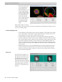
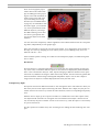
Cover illustration:
Macrophage recorded by Dr. James Evans (White-head Institute, MIT,
Boston MA, USA) using widefield microscopy, as deconvolved with
Huygens.
At the right the same dataset again: macrophage fluorescently stained
for tubulin (yellow/green), actin (red) and the nucleus (DAPI, blue).
Left part: original data; right part: as deconvolved with the classical
Maximum Likelihood Estimation method (MLE).
The image was visualized using the Simulated Fluorescence Process
(SFP) volume rendering package from Scientific Volume Imaging.
Image in figures 22, 24, 27 and 29: isolated Rat Hepatocyte couplet re­
corded by Dr. Permsin Marbet at the Department of Anatomy of the
University of Basel, Switzerland (head: Prof. Lukas Landmann), as de­
convolved with Huygens.
Image in figure 28: FISH-stained cell nucleus recorded at the Nuclear
Organization Group, SILS, University of Amsterdam, The Netherlands
(head: Prof. Roel van Driel).
This document was typeset with OpenOffice.org.
essential Doc 2.9 - 0406
Contents
Table of Contents
1. What is Huygens Essential? 1
2. Installing Huygens Essential 1
Mac OS X 1
Microsoft Windows 1
Linux 2
SGI Irix 6.5 2
IBM AIX 5.2 2
After the installation 2
The license string 2
Obtaining a license string 3
Installing the license string 3
Location of the license file 3
Trouble shooting license strings 4
Updating the software 4
Removing the software 4
System requirements for Huygens Essential 5
Windows and Linux 5
Mac OS X 5
SGI Irix, IBM AIX 5
Running the program 5
Support on installation 6
3. The image restoration process 6
The processing stages 6
Loading an image 7
Preprocessing 8
Converting a data set (optional) 8
Time series 8
Adapting the image 8
Processing brightfield images 8
Setting the image channel colors 9
Image statistics 9
Verifying the microscopic parameters 9
Parameters Templates 10
The intelligent cropper 11
Cropping an image in x y z 11
Cropping an image in time 12
Removing channels 12
Stage 1: Parameter tuning 12
Stage 2: The image histogram 12
Stage 3: Estimate the average background in the image 13
Stage 4: Deconvolution 14
The Point Spread Function (PSF) 14
The Classical Maximum Likelihood Estimation (CMLE) algorithm 15
Number of iterations 15
Signal to noise ratio 15
Quality threshold 15
Iteration mode 15
Bleaching correction 15
Stopping the MLE algorithm 16
Finishing or restarting a deconvolution run 16
z-drift corrector for time series 16
Saving the result 16
Saving the restored image 16
Saving your Task report 17
Multi channel images 17
Deconvolving a channel in a multi channel image 17
Joining the results 17
Batch processor 18
The Huygens Essential User Guide i
Contents
Start up 18
Window description 18
Usage 19
Adding one task 19
Adding multiple tasks
Running the batch job
Menus 20
File menu 20
Task menu 20
More information 20
4. Huygens Essential Visualization Tools
The Twin Slicer 21
Color mode 21
Contrast mapping mode 22
Time series 22
The MIP Renderer 23
Soft threshold 23
Rendering a movie 23
The SFP Renderer 24
Summary 24
SFP fundamentals 24
Rendering a movie 26
The Surface Renderer 26
Hue Selector 27
Transparency depth 27
19
20
21
5. Huygens Essential Analysis Tools 28
The Object Analyzer 28
How to use the Object Analyzer 28
Mouse mode 29
Frame selector 29
Render pipes 30
Object removal 30
Regions of interest (ROI) 30
Data analysis 31
Visualization parameters 32
Save the results 32
Read more 32
The Colocalization Analyzer 32
Iso-colocalization object analysis 33
How to use the Colocalization Analyzer 33
Backgrounds vs. thresholds in colocalization 35
Read more 35
6. The PSF Distiller 36
Beads for PSF distillation 36
The Distiller stages 37
Starting the Distiller 37
Parameter check stage 37
Averaging stage 37
Confocal and two photon bead images 37
Widefield bead images 38
Distillation stage 38
Assembly stage 38
7. Establishing image parameters 38
Image size 38
Brick wise processing 39
Signal to Noise Ratio (SNR) 39
Blacklevel 40
Sampling densities 40
Computing the backprojected pinhole radius 41
Airy disk as unit for the backprojected pinhole 42
Converting from integer parameter 42
Shape factor 42
Airy disk as unit for the backprojected radius of a square pinhole 43
ii Scientific Volume Imaging
Contents
Computing the backprojected pinhole distance in Nipkow spinning disks 43
Pinhole radius tables 43
Leica confocal microscopes 43
TCS 4d, SP1, NT 43
TCS-SP2 44
Zeiss confocal microscopes 44
Olympus confocal microscopes 45
Biorad confocal microscopes 45
Checking the Biorad system magnification 45
A supplied calibration curve 46
8. Improving the quality of your images 46
Data acquisition pitfalls 46
Refractive index mismatch 46
Clipping 46
Undersampling 47
Do not undersample to limit photodamage
Bleaching 47
Illumination instability 47
Mechanical instability 47
Thermal effects 48
Internal reflection 48
Deconvolution improvements 48
Acquire an experimental PSF 48
Spherical aberration correction 48
Improve the estimated parameters 48
47
9. Appendix 49
License string details 49
Questions 50
Where can I find support on the web? 50
What does the quality factor mean while running Huygens? 50
Can I deconvolve a TIFF series? 51
TIFF file series naming convention 51
Can I deconvolve a single plane widefield image? 52
Can I deconvolve a single TIFF image? 52
How do I generate a debug log? 52
Addresses and URLs 53
Where can we be reached? 53
Scientific Volume Imaging b.v. 53
Distributors 53
Support and FAQ 53
Knowledge database (FAQ) 53
The SVI-wiki 53
Starting points 53
Quick reference 54
Alphabetical Index 55
The Huygens Essential User Guide iii
Contents
iv Scientific Volume Imaging
1. What is Huygens Essential?
1. What is Huygens Essential?
Huygens Essential is an image processing software package tailored for restoration, visualization
and analysis of microscopic images. Its wizard driven user interface guides you through the pro­
cess of deconvolving images from light microscopes. Huygens Essential is able to deconvolve a
wide variety of images ranging from 2D widefield (WF) images to 4D multi-channel multi-photon
confocal images. To facilitate comparison of raw and deconvolved data or results from different
deconvolution runs the Essential is equipped with a dual 4D slicer tool. You can also render 3D
images and animations with its powerful visualization tools. Post-restoration analysis is possible
using the interactive analysis tools.
Based on the same image processing engine (the compute engine) as Huygens Professional, Huy­
gens Essential combines the quality and speed of the algorithms available in Huygens Professional
with the ease of use of a wizard driven intelligent user interface.
Huygens Essential is based on cross-platform technology. It is available on various Microsoft Win­
dows operating systems, Linux for Intel or AMD based systems, MAC OS X, IBM AIX and SGI's
Irix 6.5. For AIX and Irix 64 bit multiprocessing versions are also available.
2. Installing Huygens Essential
You can download Huygens Essential from the SVI website: http://www.svi.nl
Mac OS X
Go to the folder were you down­
loaded the distribution and
double-click on it. It will be ex­
tracted by "StuffIt Expander" to a
.pkg file, which will be placed
in the same directory. Double
click this
.pkg file, and follow the install­
ation wizard.
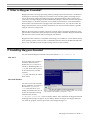
Microsoft Windows
You have received an executable
file for installation, for instance a
file named Huygense280
.exe. Place this file on your
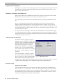
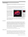
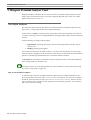
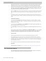
Figure 1. The start-up window on Microsoft Windows. If no license
desktop and double click its icon string is installed the software runs in 'Freeware mode'. You can find
your computer's ID number by using HELP > ABOUT
to start the installation. During
installation the directory
C:\Program files\SVI\ will be created by default. After completion the Huygens Essential
and Huygens Scripting icons appear on your desktop. Double clicking on the Huygens Essential
icon starts the program; the start-up window will be displayed (Figure 1).
The Huygens Essential User Guide 1
2. Installing Huygens Essential
Linux
The Huygens Essential Linux distribution is a 'rpm' file, for instance
huygens-2.7.0-p7.rpm. Open a Unix shell, go to the directory were this file is located,
become superuser and type: rpm -ivh --force huygens-2.7.0-p7.rpm
After installing the software type essential in a shell to start the software. A directory
/usr/local/svi will be created; initialization scripts will be installed in
/usr/local/bin.
SGI Irix 6.5
Currently the Irix distribution is a single 'tardist' file containing various components. By default
all components are installed. Become superuser and type:
swmgr -f dist65-2.7.0-p7.tardist
Press START in the Software Manager window.
After installing the software type essential in a shell to start the software. The program will
display the start-up window (Figure 1). A directory /usr/local/svi will be created; the ex­
ecutables will be installed in /usr/local/bin.
IBM AIX 5.2
Log in as root on your workstation or ask your system administrator to do so. Huygens for AIX is
distributed in a tar file. Go to the directory where you downloaded it to. After unpacking the distri­
bution file with tar xvf my_aixfile.tar you will find three new files: svi.tar.Z,
README.AIX and a shell script AIX-install.sh. To install the software you have to run the
file AIX-install.sh by typing ./AIX-install.sh. This script will unpack the
svi.tar.Z file under /usr/local and then will do some post installation tasks and verifica­
tion. After a successful installation it will print the message "OK." to the screen.
A directory /usr/local/svi will be created; the executables will be installed in
/usr/local/bin.
After the installation
After a first-time installation there is not yet a license available. Still, you can start the software.
Without a license it will run in 'Freeware mode'. Among others, this gives you access to the Li­
cense tools in the HELP menu. The next section explain how to obtain and install a license string.
On AIX, Irix and Linux start the software by clicking its icon or by typing essential into a
Unix shell. On Mac OS X and Windows click its icon. The software will open in Freeware mode
and display the start-up window (Figure 1).
The license string
The license key used by all SVI software is a single string per licensed package. It may look as fol­
lows:
HuEss-2.7-wcnp-d-tv-emnps-eom2008Dec31-e7b7c623393d708e{[email protected]}-4fce0dbe86e8ca4344dd
At startup Huygens Essential searches for a license file huygensLicense which contains a li­
cense string. This license string is provided by SVI via e-mail. Installing the license string is the
same for all platforms, though on Linux, Irix and AIX only the superuser can do this.
2 Scientific Volume Imaging
2. Installing Huygens Essential
Obtaining a license string
If you are not upgrading from a previous installa­
tion it is likely that a license is not yet available. To
enable us to generate a license string for you we
need the fingerprint of your computer, the system
ID number. If you have not done so already, start
Huygens Essential. The system ID is displayed in
the HELP > ABOUT dialog (Figure 2). Send it to
[email protected], and you will be provided with a
license string. To prevent any typing error use the
COPY button to save the ID to the clipboard. You
can print it into your mail message with the EDIT >
PASTE menu item of your mail program.
In this dialog box you can also find a button to
CHECK FOR HUYGENS UPDATES on our company server.
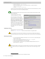
Installing the license string
Figure 2 The HELP > ABOUT window. The
system ID is shown at the bottom.
Select the license string in your email message and
copy it to the clipboard using EDIT > COPY in your mailing program. Start Huygens Essential and
go to HELP > LICENSE: a dialog box pops up (Figure 3). Then press the ADD A NEW LICENSE button
and a new window will pop up (Figure 4). Paste the string into the text field using your keyboard1.
Complete the procedure using the ADD LICENSE to add the string to the huygensLicense file.
Please try to avoid typing the license string by hand: any small typing error will invalidate the li­
cense. With an invalid license, the software will remain in Freeware mode.
Figure 3. The License manager dialog. Left: as displayed on Mac OS X; right: as displayed on Irix.
The License manager allows you to add, delete and troubleshoot licenses.
Figure 4. The Add License dialog box.
Location of the license file
The license string is added to the file huygensLicense in the svi directory. On the different
supported platforms this is located in:
1
Use your operating system's generic copy / paste operations: Mac OS X: apple-c / apple-v; Windows:
control-c / control-v; Linux, Irix, Aix: on most common desktops copying is done simply by marking the
text area with the mouse, and pasting by either middle mouse click or control-v.
The Huygens Essential User Guide 3
2. Installing Huygens Essential
•
•
•
AIX, Irix and Linux: /usr/local/svi
Mac OS X: depends on where you installed the software. A typical example is
/Applications/SVI
Windows: C:\Program Files\SVI\
On AIX, Irix and Linux and Mac OS X an alternative location is the user's home directory. On OS
X this is especially convenient when updating frequently.
Restart Huygens Essential to activate the new license. This will enable the deconvolution or PSF
distiller functionality.
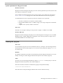
Trouble shooting license strings
The license string as used by SVI has
the same appearance on all supported
platforms. For each product2 you need to
have a license string installed. Select a
license string in the License manager
and press the EXPLAIN LICENSE button. All
details for the current license will be lis­
ted. If you run into licensing problems
you may use this information to analyze
the problem. See License string details
on page 49.
Updating the software
Figure 5. The License details.
Download the new version from the SVI
website at http://www.svi.nl. Proceed with the installation as explained above.
Do not uninstall the old version as this will delete your license string. On Mac OS X make sure
you make a backup of the license string in a safe place before you remove the previous installation.
Removing the software
•
•
•
•
Irix: Open the Software Manager, select MANAGE INSTALLED SOFTWARE, and mark the pack­
ages you wish to remove.
Linux: To remove Huygens Essential type as root: rpm -e huygens
Mac OS X: Drag the installation to the waste basket.
Microsoft Windows: Clicking START in your Windows desktop and select: PROGRAMS >
HUYGENS ESSENTIAL > UNINSTALL.
Removing the software will also cause your license string to be removed. If you prefer to uninstall
your current version prior to installing a newer one, be sure to store your license string in a safe
place.
2
Huygens Essential, Huygens Professional and Huygens Scripting.
4 Scientific Volume Imaging
2. Installing Huygens Essential
System requirements for Huygens Essential
Windows and Linux
Huygens Essential and Huygens Scripting run on the following Windows operation systems: Win­
dows 2000, NT, 2003 Server and XP.
Linux: RedHat and SuSE distributions. Since Linux versions evolve rapidly best consult SVI's
http://www.svi.nl web page to see which Linux distributions are currently supported.
A standard Ethernet card is required to provide your computer with a system ID.
•
•
•
Processor: Pentium III or IV (Intel) or Athlon (AMD).
Recommended RAM memory: 512 MB or larger (to run larger images like 512*768*50
voxels).
Graphics card: any fairly modern card will do.
Mac OS X
Mac OS X 10.2 or higher running on a G4 processor or higher. 512 MB or more RAM.
SGI Irix, IBM AIX
Huygens Essential and Huygens Scripting run on all SGI equipment running Irix 6.5 on a MIPS
R5000 processor or higher, IBM AIX 5.2 equipment with a Power4 processor or higher. The re­
commended RAM size is 512 MB or larger.
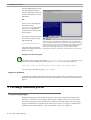
Running the program
Mac OS X
You can find the program icon in the installation directory. Clicking it will start Huygens Essen­
tial and open the main window (Figure 6). You can also run the program by typing essential
at a shell prompt.
Windows
The Windows installation procedure has automatically placed an Huygens Essential icon on your
desktop. Clicking it will start Huygens Essential and open the main window (Figure 6).
Linux
On Linux you can start Huygens Essential by typing essential at a shell prompt. It will start
Huygens Essential and opens the main window (Figure 6).
If the shell is unable to find this command then typing the full path should help:
/usr/local/bin/essential
If this still does not help then Huygens Essential has not been installed correctly.
The Huygens Essential User Guide 5
2. Installing Huygens Essential
In Linux KDE desktop you may
also start Huygens Essential
from the Application menu and
in the Gnome desktop from the
Main Menu.
Irix
On Irix you can start Huygens
Essential by typing
essential at a shell prompt
which will start Huygens Es­
sential and opens the main win­
dow (Figure 6).
If the shell is unable to find this
command then typing the full
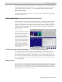
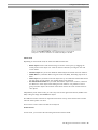
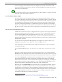
Figure 6. The start-up window. The gray area in the upper part is the
path should help:
/usr/sbin/essential
If this still does not help then
Huygens Essential has not been
installed correctly.
work area where the thumbnail representation of the original image
and its individual channels will be placed. The blue window in the left
will show help text, task reports and supporting information during the
various processing stages. In the gray bottom right field different
dialog boxes will appear during processing. Also intermediate
deconvolution results are shown here. The bottom bar is a status area.
Adding to the shell search path
Users of the csh or tcsh shell can add the /usr/local/bin or /usr/sbin/ directory to their
shell search path by adding the following line to the .cshrc file in their home directory:
set path=(/usr/local/bin $path) or set path=(/usr/sbin $path)
You can inquire your shell by typing: echo $shell
Support on installation
If you find any problem in installing the program or the licenses that you could not solve with the
guidelines here included, please search the knowledge database or contact SVI on the addresses on
page 53.
3. The image restoration process
The processing stages
Huygens Essential guides you through the process of microscopic image deconvolution (also re­
ferred to as 'restoration') in several stages. Each stage is composed of one or more tasks. While
proceeding each stage is briefly described in the bottom-left Task Info window pane. The stages
progress is indicated at the right side of the status bar (see Figure 15 on page 13). Additional in­
formation can be found in the HELP > QUESTIONS and HELP > DICTIONARY (Figure 7).
6 Scientific Volume Imaging
3. The image restoration process
The following steps and stages are to be
followed:
•
•
•
•
•
•
•
Opening an image. A demo im­
age (the faba64.ics/ids
file pair) is placed in the
images subdirectory of svi.
stage P: The Preprocessing
stage: loading an image, con­
verting data sets, parameter
check and cropping.
stage 1: Tune the parameters.
This stage will be skipped when Figure 7. The Dictionary. The DICTIONARY and the QUESTIONS
you entered from the prepro­
from HELP give additional information.
cessing stage. In the prepro­
cessing stage you have already checked the parameter settings for the intelligent cropper intelligent since it uses a-priori knowledge for setting the optimal cropping boundaries
automatically. You will enter this stage from the latest one when clicking the <<RESTART
button. This is useful if you wish to fine tune your parameters for the best deconvolution
result, in particular when you like to set your parameters slightly different when using
multi-channel images (see page 17).
stage 2: Inspecting the image histogram.
stage 3: Background estimation.
stage 4: The deconvolution run.
saving the result.
The different stages will be explained below
Loading an image
Select OPEN from the FILE menu to enter the file browser and move to the directory where your im­
ages are stored. Select the image to be deconvolved, e.g. the faba64.ics/ids file pair in the
images subdirectory of svi.
Several formats from microscope vendors are supported. If you have TIFF images to be processed
please read TIFF file series naming convention on page 51 for the naming convention in order to
be able to read a multi-dimensional image as a whole.
When the file is read successfully you can either press START DECONVOLUTION to begin processing
your image or you can convert your data set with the TOOLS button.
If you have loaded a bead image you also can proceed selecting START PSF DISTILLER and proceed
with generating a Point Spread Function (PSF, see page 14) from measured beads (See The PSF
Distiller on page 36).
A special license is needed in order to launch the PSF Distiller.
You can OPEN ADDITIONAL images for reference purposes, but only the one named 'original' will be
deconvolved during the guided restoration.
The Huygens Essential User Guide 7
3. The image restoration process
Preprocessing
Converting a data set (optional)
Before you press the START DECONVOLUTION button you can convert a 3D stack into time series im­
ages (Convert XYZ to XYZT) or vice versa, or you can convert a 3D stack into a time series of 2D
images (XYZ to XYT) or vice versa. These functions can be found in the TOOLS.
Hint: If you have a data stack that is poorly sampled in z (not fulfilling the Nyquist criterion) you
better interpret the different planes as independent (i.e. as 2D images) and do 2D deconvolution
planewise while taking the optimal Nyquist criterion for z as imposed by the optical parameters
(see the diagram in , page ). To do this in one run for all the planes, convert the 3D stack to a 2Dtime series, do the deconvolution run, and convert back from 2D-time to 3D.
Time series
A time series is a sequence of images recorded along time at uniform time intervals. Every recor­
ded image is a time frame. The Huygens Essential is capable of automatic deconvolution of 2Dtime or 3D-time data. There are some tools that are intended only for time series, as the confocal
bleaching corrector or the z-drift corrector (page 16).
Adapting the image
In the TOOLS menu you can find a contrast inverter helpful for the processing of brightfield images,
see below.
A CROP tool is also available, but its use is recommended only after properly tuning the image
parameters and will be explained in a later stage.
In the TOOLS menu you can also find a MIRROR ALONG Z tool, to flip the image when the coverslip is
in the top. This is specially important in case of a refractive index mismatch: see Spherical aber­
ration correction on page 48.
Processing brightfield images
Brightfield imaging is not a 'linear imaging' process. In a linear imaging process the image forma­
tion can be described as the linear convolution of the object distribution and the point spread func­
tion (PSF, see page 14), hence the name deconvolution for the reverse process. So in principle one
cannot apply deconvolution based on linear imaging to non linear imaging modes like brightfield
and reflection. One could say the image formation in these cases IS linear because it is governed
by linear superposition of amplitudes. However, microscopes do not measure light amplitudes but
rather intensities, the absolute squared values of the amplitudes. Taking the absolute square des­
troys all phase information one would need to effectively apply deconvolution. Fortunately, in the
brightfield case the detected light is to a significant degree incoherent. Because in that case there
are few phase relations the image formation is largely governed by the addition of intensities, es­
pecially if one is dealing with a high contrast image.
In practice one goes about deconvolving brightfield images by inverting them (using TOOLS >
INVERT IMAGE) and processing them further as incoherent fluorescence widefield images. Still, one
should watch out sharply for interference like patterns (periodic rings and fringes around objects)
in the measured image. As a rule these become pronounced in low contrast images. After the de­
convolution run you may reverse to the original contrast setting.
8 Scientific Volume Imaging
3. The image restoration process
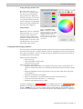
Setting the image channel colors
The Color picker tool (TOOLS >
SET CHANNEL COLORS) allows you to
alter the colors for the different
image channels (see Multi chan­
nel images on page 17). The color
of a particular channel can be ed­
ited by clicking the corresponding
button. This opens a platform spe­
cific color editor (Figure 8).
Image statistics
Right-mouse-click on a thumbnail
image and select SHOW PARAMETERS
and you will find, besides the
parameter settings, statistical in­
formation of the particular image.
Amongst them are the mean, sum,
standard deviation, norm, and po­
sition of the center of mass.
Figure 8. The Image Color
Picker. Clicking on a channel
button (top) opens a color editor
(right) by which the color can be
changed. The color editor is
platform specific. The picture on
the right shows the Mac OS X
color editor.
Verifying the microscopic parameters
Next to the basic voxel data the Huygens Essential also tries to read as much as possible informa­
tion about the microscopic recording conditions. However, depending on the file type this inform­
ation may be incomplete or incorrect. In this first stage all parameters relevant for deconvolution
are displayed and can be modified:
Optical parameters (first page):
• Microscope type
• Lens and medium refractive index
• Numerical Aperture (NA)
Optical parameters (second page):
• Backprojected pinhole radius in nm. 'Backprojected' means the size of the pinhole as it
appears in the specimen plane, see Computing the backprojected pinhole radius on page
41.
• Backprojected distance between the pinholes in microns (only visible if the microscope
type is 'Nipkow').
• Excitation and emission wavelengths
• Photon count (number of excitation photons involved in the fluorescence)
• Voxel sizes in the three directions x, y, z (third page)
• Summary of all parameters now in effect
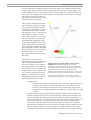
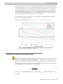
If values are displayed in a red background , they are highly suspicious. An orange background
indicates a non-optimal situation. Oversampling is also indicated with a cyan background , that
becomes violet when it is very severe. Figure 9 shows settings which do not fulfill the criterion
for the critical sampling distance versus numerical aperture. (See Sampling densities on page 40).
The Huygens Essential User Guide 9
3. The image restoration process
You can see and correct the image
parameters not only at this decon­
volution stage, but also at any time
by right-clicking on the image
thumbnail and selecting SHOW
PARAMETERS or CORRECT PARAMETERS.
Correcting will pop up the window
shown on Figure 11.
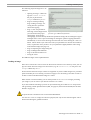
Parameters Templates
Once the proper parameters have
been set and verified, they can be
saved to a Huygens template file
(suffix .hgst). Those template
files are loadable in the very start
Figure 9. Parameters check stage: Sampling. Red coloring
indicates a suspicious value, and orange a non-optimal value.
of the wizard, hence the user can
skip the parameters verification
stage, provided that an image is to be restored with the same optical properties as the ones which
were recorded on the template.
Figure 10. Importing a microscopical parameters template.
The IMPORT MICROSCOPIC TEMPLATE button will allow you to choose a
template from a list of pre-saved template files which reside both in
the common templates directory and in the user's personal template
Figure 11. Microscopical
directory. The Huygens common templates directory is named
parameters corrector.
Templates, and resides in the Huygens installation directory,
namely /usr/local/svi/Templates on Unix systems, C:\Program
Files\SVI\Templates on Windows and /Applications/SVI/Templates on the Mac
OS X. The user's personal templates directory is called .svi on the Unix platforms and SVI
on Windows, and it can be found in the user's home directory on Unix, and in C:\Documents
and Settings\user_name on Windows. You can also choose to load a template file from a
different location by pressing the FROM DISK... option.
10 Scientific Volume Imaging
3. The image restoration process
The EXPORT TEMPLATE button will al­
low you to either save the template
to the personal template directory
by choosing the TO DISK... option, or
overwrite one of the existing tem­
plates by selecting them from the
list.
The Huygens template is a simple
.xml file which can be edited 'by
hand' as well (see examples in the
common Templates directory).
The intelligent cropper
The time needed to deconvolve an
Figure 12. Exporting a microscopical parameters template.
image increases more than propor­
tional with its volume. Therefore, deconvolution can be accelerated considerably by cropping the
image. Huygens Essential is equipped with an intelligent cropper which automatically surveys the
image to find a reasonable proposal for the crop region. In computing this initial proposal the mi­
croscopical parameters are taken into account, making sure that cropping will not have a negative
impact on the deconvolution result. Because the survey depends on accurate microscopical para­
meters it is recommended to use the intelligent cropper as final step in the preprocessing stage, but
you can launch it before the restoration process from the TOOLS > CROP ORIGINAL IMAGE menu. Once
you have cropped your image during the guided restoration process you can not crop it again ex­
cept after closing the image and reloading it again.
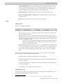
Cropping an image in x y z
After you have verified your image parameters the Crop tool is launched if you press the YES but­
ton to the question 'Launch the cropper?'. The cropper will look as in Figure 13 (the image will be
in gray scale mode if it is a single channel). Red lines indicate the borders of the proposed crop­
ping region. This is computed from the image content and the microscopic parameters at launch
time of the cropper.
The cropper allows manual adjustment of the proposed crop region. To adjust the crop region put
the cursor inside the red boundary, press the left mouse button and keep it pressed to sweep out a
volume. Accept the new borders by pressing the CROP button. Do not crop the object too tightly,
because you would remove blur information relevant for deconvolution. Do not crop the image to
make it too large along the optical axis Z, an aspect ratio close to 1:1:1 (or less than 1 for Z) is
much better.
The three views shown are Maximum Intensity Projections (MIP's) along the main axes. The pro­
jections are computed by tracing parallel rays perpendicular to the projection plane through the
data volume, each ray ending in a pixel of the projection image. The maximum intensity value
found in each ray path is projected. For example, each pixel in the xy projection image corres­
ponds with the maximum value in the vertical column of voxels above it.
By default the projections are over the whole dataset (including all the frames in time series), but
this might be confusing sometimes. The small colored triangles can be used to restrict the projec­
tions within a specific range of slices.
The Huygens Essential User Guide 11
3. The image restoration process
Cropping an image in time
You also can reduce the number of time
frames by selecting TIME > SELECT FRAMES
from the CROP menu, as shown in Figure
14. This applies to time series (see Time
series on page 8).
Removing channels
You can remove channels from a multichannel image (see p. 17) using the crop
tool's channels selecting tool CHANNELS >
SELECT CHANNELS.
Stage 1: Parameter tuning
Stage 1 enables you to tune your para­
meter settings as set in the pre-pro­
cessing stage. After you have finish
cropping stage 1 is skipped and you will
directly jump into the image histogram
(stage 2). Still you may wish to tune
your parameter settings afterwards. You
can enter stage 1 by pressing the RESTART
button in the latest stage.
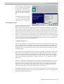
Stage 2: The image histogram
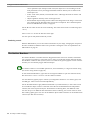
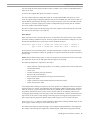
Figure 13. The Crop tool.
The next stage shows you the image histogram.
The histogram image is an important statistical tool for inspecting your image. It is included to let
you spot problems that might have occurred during the recording. It has no image manipulation
options as such, it just may prevent you from future recording problems.
The histogram shows the number of pixels as a function of the in­
tensity (gray value) or groups of intensities. If your image is an 8bit image (gray values from 0−255) the x-axis is the gray value and
the y-axis is the number of pixels in the image with that gray
value. If the image is more than 8-bits gray values are collected to
form a 'bin' (for example gray values from 0−9 form bin 0, values
from 10−19 form bin 1, etc.) The histogram is now the number of
pixels in every bin.
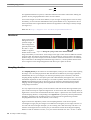
The histogram from the demo image as shown in Figure 15 is of
Figure 14. Reducing the
reasonable quality. The narrow peak you see at the left represents
number of time frames.
the background pixels, all with similar values. The height of the
peak represents the amount of background pixels. Because in this particular image there are many
voxels with a value in a narrow range around the background the peak is higher than the other.
In this case there is also a small black gap at the left of the histogram. This signifies an electronic
offset (blacklevel) in the signal recording chain of the microscope (see page 40).
If a peak is visible at the extreme right hand side of the histogram it indicates saturation or 'clip­
ping'. Clipping is caused by intensities above the maximum digital value available in your micro­
scope. Usually, all values above the maximum value are replaced by the maximum value. On rare
12 Scientific Volume Imaging
3. The image restoration process
occasions they are replaced by
zeros. Clipping will have a negat­
ive effect on the results of decon­
volution, especially with WF im­
ages. (See page 46).
The histogram stage is included
for examining purpose only. It
has no meaning for the deconvo­
lution process that follows3.
Stage 3: Estimate the average background in the
image
In this stage the average back­
ground in a volume image is es­
timated. The average background
is thought to correspond with the
noise-free equivalent of the back­ Figure 15. The image histogram. The vertical mapping mode can be
selected from linear, logarithmic or sigmoid.
ground in the measured (noisy)
image. It is determined by searching the image first for a region with low values. Subsequently the
value for the background is determined by searching in this region for the area with radius r
which has the lowest average value. It is important for the search strategy that the microscopic
parameters of the image are correct, in especially the sampling distance and the microscope type.
The following choices are possible here:
•
•
•
Lowest value (Default):
The image is searched
for a 3D region with the
lowest average value.
The axial size of the re­
gion is around 0.3 mi­
cron; the lateral size is
controlled by the radius
parameter which is de­
fault set to 0.5 micron.
In/near object: The
neighborhood around the
voxel with the highest
value is searched for a
planar region with the
Figure 16. Estimating the average background.
lowest average value.
The size of the region is
controlled by the radius parameter.
WF: First the image is searched for a 3D region with the lowest values to ensure that the
region with the least amount of blur contributions is found. Subsequently the background
is determined by searching this region for the planar region with radius r that has the
lowest value.
Press the ESTIMATE button to continue. You may now adapt the value if you like to, either by alter­
ing the value in the ESTIMATE BACKGROUND field or in the RELATIVE BACKGROUND field. Setting this last
3
Learn more about histograms in http://support.svi.nl/wiki/ImageHistogram
The Huygens Essential User Guide 13
3. The image restoration process
to -10, for example, lowers the estimated background with 10%. If you are done press ACCEPT to
start the last stage, the true deconvolution process.
Stage 4: Deconvolution
Before starting the actual iterat­
ive deconvolution run, stage 4
first carries out several prepro­
cessing steps:
1. Background: This value
is calculated in stage 3.
You can verify whether
this value represents
areas in the image which
you consider background
by opening the Twin
Slicer (see Figure 21)
and moving the mouse
pointer over the areas of
interest. The voxel val­
ues are displayed below Figure 17. Stage 4: starting the deconvolution.
the image. Modify the
value as you see fit.
2. A Point Spread Function (PSF, see below) was generated from the established microscop­
ic parameters. This took place off the screen and is fully transparent to the user.
3. If the size of the computer's RAM is too small to deconvolve the image as a whole, it is
split up in parts called 'bricks'. SVI's Fast Classic Maximum Likelihood Estimation
(MLE) algorithm runs on the image or on all the bricks and fits the deconvolved bricks
seamlessly together (see Brick wise processing on page 39).
The Point Spread Function (PSF)
One of the basic concepts in image deconvolution is the Point Spread Function. The PSF of your
microscope is the image which results from imaging a point object in the microscope. Due to wave
diffraction a point object is imaged, 'spread out', into a fuzzy spot: the PSF. In fluorescence ima­
ging the PSF completely determines the image formation. In other words: all microscopic imaging
properties are packed into this 3D function. The PSF can be obtained in two different ways:
1. Generating a theoretical PSF: When a measured PSF is not available, Huygens Essen­
tial automatically uses a theoretical PSF. The PSF is computed from the microscopic
parameters that come with your image and which you have double-checked in the prepro­
cessing 'P' stage or in stage one. Because a theoretical PSF can be generated without any
user intervention Huygens Essential does the calculation in the background without any
notice.
Images affected by spherical aberration (S.A.) due to a refractive index mismatch are better re­
stored through the use of theoretical depth-dependent PSF's. Read about S.A. on page 46, and how
to correct it on page 48.
2. Measuring a PSF: By using the PSF Distiller or the tools in Huygens Professional you
can derive a measured PSF from images of small (< 200 nm) fluorescent beads.
You can load a previously measured PSF with FILE > OPEN PSF... (Main menu). If you
load a PSF, Huygens Essential will automatically use it. If the measured PSF contains less
14 Scientific Volume Imaging
3. The image restoration process
channels than the image, a theoretical PSF will be generated for the channels where there
is no PSF available.
See The PSF Distiller on page 36 for more information on measuring a PSF.
A measured PSF should only be used for deconvolution if the image and the bead(s) were recorded
with the same microscope at the same parameter settings as the bead image(s).
The Classical Maximum Likelihood Estimation (CMLE) algorithm
Huygens Essential uses the Classical Maximum Likelihood Estimation for the deconvolution pro­
cess. This method is an extremely versatile algorithm, applicable for all types of data sets4.
The following option values may be set:
Number of iterations
MLE-based deconvolution uses an iterative process that never stops if no stopping criterion is giv­
en. This stopping criterion can simply be a maximum number at which the process will stop. This
value depends on the desired final quality of your image. For an initial run you can leave the value
at its default. To achieve the best result you can increase this value.
Another stopping criterion is one based on the Quality change of the process, see Quality
threshold below.
Signal to noise ratio
You have to make an estimation of the SNR from your recorded image. Inspect your image and
decide if your image is noisy (SNR < 10), has moderate noise (10 < SNR < 20) or is a low-noise
image (SNR > 20). See Signal to Noise Ratio (SNR) on page 39, and some examples of noisy im­
ages in Figure 31.
Quality threshold
Beyond a certain amount of iterations, typically below 100, the difference between successive iter­
ations becomes insignificant and progress grinds to a halt. Therefore it is a good idea to monitor
progress with a quality measure, and to stop iterations when the change in quality drops below a
threshold. At a high setting of this quality threshold (e.g. 0.1) the quality difference between sub­
sequent iterations may drop below the threshold before the indicated maximum number of itera­
tions has been completed. The smaller the threshold the larger the number of iterations which are
completed and the higher the quality of restoration. Still, the extra quality gain becomes very
small at higher iteration counts.
Iteration mode
In FAST MODE (highly recommended) the iteration steps are bigger than in HIGH QUALITY mode.
More information can be read in the DICTIONARY from the HELP menu.
Bleaching correction
The data is inspected for bleaching. 3D images and time series of WF images will always be cor­
rected. Confocal images can only be corrected if they are part of a time series, and when the
bleaching over time shows exponential behavior.
4
Huygens Professional also has Quick-MLE-time, Quick-Tikhonov-Miller, and Iterative Constrained
Tikhonov-Miller.
The Huygens Essential User Guide 15
3. The image restoration process
Stopping the MLE algorithm
Pressing RESTORE starts the iterative MLE algorithm; a STOP button appears. Pressing STOP halts the
iterations and retrieves the result from the previous iteration. If the first iteration is not yet com­
plete a empty image will result.
Finishing or restarting a deconvolution run
When a deconvolution run is finished use the Twin Slicer (page 21) to inspect the result in detail.
Depending on the outcome of that you can choose AGAIN, RESUME or ACCEPT:
AGAIN discards the present result, and re-runs the deconvolution, possibly with different paramet­
ers.
RESUME re-runs the MLE procedure without discarding the result, and with the possibility to
change the deconvolution parameters. The software will ask you to continue were you left off
(keeping improving the image, quite recommendable) or to start from the raw image again. A new
result will be generated to compare with the previous one, for instance using the Twin Slicer. You
can repeat this several times.
ACCEPT proceeds to the final stage or, if the data was multi-channel, to the next channel (see page
17). If you generated several results by resuming the deconvolution you will be asked to select the
best result as the final one, that will be renamed to 'deconvolved'. The other results will remain as
well in case you want to save them.
z-drift corrector for time series
For 3D time series the program pops-up an
additional tool that enables you to correct for
movement in the z (axial) direction that could
have been occurred for instance by thermal
drift of the microscope table. In case of a
multi channel image (see p. 17), the corrector
can survey ALL CHANNELS and determine the
mean z position of the channels, or it can take
ONE CHANNEL as set by the REFERENCE CHANNEL
parameter.
After determining the z positions per frame,
the z-positions can be filtered with a MEDIAN,
GAUSSIAN or KUWAHARA filter of variable width. Figure 18. The z-drift corrector.
When the drift is gradual, a gaussian filter is
probably best. In case of a drift with sudden reversals or outliers a median filter is best. In case the
z positions show sudden jumps, we recommend the edge preserving Kuwahara filter.
Saving the result
Saving the restored image
After each deconvolution run you can save the result. Select the image to be saved and do FILE >
SAVE 'IMAGENAME' AS... in the menu bar. You can save the image as an Image Cytometry Standard
(ICS or ICS2) image file, a TIFF file series, an Imaris-Classic file or a Biorad .pic file. Only the
ICS and ICS2 file type save all the microscopic parameters. For information on how to proceed
with multi-channel data see Joining the results on page 17.
16 Scientific Volume Imaging
3. The image restoration process
The ICS file format actually uses two separate files: a header file with .ics extension and other,
much bigger and with the actual image data, with .ids extension. On the other hand the newer
ICS2 file format uses only one single .ics file with both the header and the data together.
Saving your Task report
Select from the Main menu bar TASK > SAVE TASK REPORT to store the information as displayed in
your Task report tab deck.
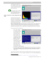
Multi channel images
Fluorescent microscopes can usually register different emission wavelengths (almost) simultan­
eously, allowing you to image different dyes on the sample. In the terminology of the Huygens
Software, one channel in an image refers to the intensity distribution recorded at a given fixed
wavelength, independently of what device made the acquisition. Thus, it is a logical channel of
stored data, and not necessarily a physical channel (as all the image channels could have been
measured by a single photomulti­
plier, for instance).
Multi channel images can be de­
convolved in a semi automatic
fashion, giving you the opportun­
ity to fine tune the results ob­
tained with each individual chan­
nel. After the preprocessing
stage the multi channel image is
split into single channel images
named 'channel-0', 'channel-1',
and so on. The first of these is
automatically selected for decon­
volution. To deconvolve it, pro­
ceed as follows:
Deconvolving a channel in a multi channel image
Figure 19. Deconvolving a two channel image.
The procedure to deconvolve a channel in a multi channel data set is exactly the same as for a
single channel image. You can therefore do multiple reruns on the channel at hand, just as you
can with single channel data. When you are done press ACCEPT in the last (stage 4) screen. This
will cause the next channel to be selected for restoration. Proceed as usual with that channel and
the remaining channels. If you do not want to process all the channels in an image you may skip
one or more channels.
Joining the results
When you press ACCEPT for the last channel you enter a screen which allows you to select the res­
ults which you want to combine into the final deconvolved multi channel image. This means that
up to this point you can still change your mind as to which of the results you want to combine,
even in what order. Once you press ACCEPT a multi channel image named Restored is created. To
save it go to the FILE > SAVE 'RESTORED' AS menu.
The Huygens Essential User Guide 17
3. The image restoration process
Batch processor
Once you know how to deal with a particular kind of dataset and are sure of the restoration para­
meters (see Improve the estimated parameters on page 48), you can restore a couple or more of
similar datasets automatically. This is called batch processing.
A batch process is made of independent image restoration tasks (one per image) that are executed
one by one until all are finished. Depending on the multithread capabilities of the computer mul­
tiple tasks can be executed in parallel.
You can for example program batch scripts using Huygens Scripting, that enables you to run
scripts written in Tcl, using the extensive set of Tcl-Huygens image processing commands.
You can also configure batch processes easily using the interactive Huygens Batch Processor. The
Batch Processor is the tool to do large scale deconvolution of multiple images within the Huygens
Essential.
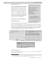
Start up
To launch the Batch Processor first open Huygens Essential, then click on the menu
DECONVOLUTION > BATCH PROCESSOR.
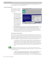
Window description
These are the different elements that form the window:
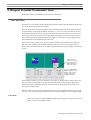
Figure 20: Batch Processor main window.
•
18 Scientific Volume Imaging
Save location is the location where the resulting images will be placed during the batch
run. With the two folder buttons you can respectively select a location or create a new one
in the currently selected folder.
3. The image restoration process
•
Current task lines shows a list of tasks (empty at start). Tasks are jobs that will be pro­
cessed by the Batch Processor one by one. Each task line consists of an image, a micro­
scopic template and a deconvolution template. These templates can be updated after a
task line is added to the list to tune the values in each particular case.
•
Add Task Line(s) to add tasks to the list, one by one or many at the same time.
•
The text tabs (Info, Progress, and Report) give information about the whole process in
its different stages.
•
Run button, to launch the process when everything is configured.
Usage
Adding one task
First let us try adding a single task:
•
•
•
•
Click on SELECT AN IMAGE FILE... and browse to select one raw image that you want to de­
convolve. End by clicking OPEN.
Then click on MICRO TEMPLATE... to load on the microscopic parameter set that you use in
Huygens Essential. If none exists, you must CREATE one. The CREATE actually opens a tem­
plate editor, where you can load and save many different templates (overwriting the exist­
ing ones, or creating new ones).
• Tip: prepare your templates in the Huygens Essential main window before select­
ing them in the Batch Processor (see page 10). This will allow you to use the
parameters saved inside an image.
Repeat the same procedure with the DECON TEMPLATE... to establish a set of restoration para­
meters. In the Batch Processor, appart from the wizard CMLE restoration algorithm, you
can also use the QMLE, a quicker version that works very well with low noise images5.
Finally, the icon with the single green plus sign will be enabled: click on it to add the
task.
You will see the task included in the list of tasks. By now it is the only one, we will add more
later. You can now click on the different task elements:
•
the image name, to change the data file the task is executed with.
•
the microscopic template, to change the microscopic parameters You can modify them or
load a new template.
•
the deconvolution template, to change the restoration parameters. You can modify them
or load a new template.
•
the "trash can" icon, to remove the task from the list.
Adding multiple tasks
Now that you have learnt how to add one task to the job list and explored its capabilities, we can
speed things up and add many tasks at the same time.
5
See http://support.svi.nl/wiki/RestorationMethod for more information.
The Huygens Essential User Guide 19
3. The image restoration process
You can use the button with the two plus signs for that:
That will open a new dialog, where you can select multiple images that will be deconvolved with
the same microscopic and restoration templates, as specified.
You can add all image files present in a directory, or add multiple files. In the second alternative,
multiple files can be selected by holding down the control key (apple in the Mac). Once you have
accepted a list with all the images, select the templates to be used with them, and click ADD to
generate all the task lines. All of them will use the selected templates.
Repeat the procedure to add more image or use different templates. Click CANCEL to finish.
When you change one task's template you see that the template name is also changed, indicating
that some parameters were modified locally. These changes do not affect the template as it is used
by the other tasks.
Running the batch job
Make sure you selected the desired location to save the results.
When you have your batch process configured, you can save it for future reference: in the menu,
do FILE > SAVE.
When everything is ready you just click the RUN button to start the jobs.
The progress of the Batch Processor and the report for each individual task are shown on the text
tabs of the Batch Processing Overview. The status of each task on the task list changes accord­
ingly to the evolution of the process.
The restored images are saved on the selected destination directory as soon as they are ready.
Menus
File menu
By using this menu you can CLOSE the current process, create a NEW task list, OPEN previously
saved processes and SAVE them to the disk, or APPEND other task lists to the current one.
You can also EXIT the Processor.
Task menu
By using this menu you can RUN the tasks, and SAVE BATCH PROGRESS or SAVE BATCH REPORT to text
files on the disk.
More information
Updated information about the Batch Processor can be found in
http://support.svi.nl/wiki/BatchProcessor.
20 Scientific Volume Imaging
4. Huygens Essential Visualization Tools
4. Huygens Essential Visualization Tools
Huygens Essential provides different tools for data visualization.
The Twin Slicer
This allows you to compare a deconvolution result with the original, but also different deconvolu­
tion results obtained from the same original.
Open the Twin Slicer by double clicking on one of the thumbnail images in the main window (or
by right-clicking on the image thumbnail, then SHOW ON TWIN SLICER). The Twin Slicer will show
the selected image on the left. By clicking on the menu bar below the image you can select a dif­
ferent image. Likewise, the bar below the right display field gives access to one of the other im­
ages currently present in Huygens Essential (see Figure 21). Currently only two images with the
same dimensions can be displayed at the same time.
If you select the same image twice, you may compare different slices from the same image. For
this, first move the slider until the desired position, then click on one of the image's name to
DISABLE the action of the slider on it: the slider will then affect only the other image view (see Fig­
ure 22).
Click the name
button to select an
image, disable the
slider function or
center the image.
Figure 21. The Twin
Slicer, applied to a 3D
dataset. The selected
display settings are
highlighted in blue.
Pixel intensity values for the cursor position on the image are displayed at the bottom of the win­
dow. You can move the image by clicking the left-mouse button and keeping it pressed while
moving the image to the desired position. You can center the image again by selecting CENTER
IMAGE from the name button.
With the slider you can slice your images along the three axis, depending on what is the selected
slice view. You can also change the zoom factor, the color mode and the contrast mapping mode.
Color mode
•
Gray: pixel values are assigned different shades of gray ranging from black for the lowest
values to white for the highest values.
The Huygens Essential User Guide 21
4. Huygens Essential Visualization Tools
•
•
False color: pixels values
are assigned different
colors ranging from
black/dark purple for the
lowest values to bright
red for the highest value.
True color: pixel values
are assigned different
shades of a particular
color ranging from black
for the lowest values to
the brightest possible
shade for the highest
values.
Figure 22. The Twin Slicer showing two slices of the same 3D image.
Multi channel images are always
rendered with a true color scheme, otherwise the information from the different channels will res­
ult in very confusing images.
Contrast mapping mode
•
•
•
Linear (default): In this mode the pixel values are mapped to screen buffer color intensit­
ies in a linear fashion. Note that the actual translation of the screen buffer values to the
actual brightness of a screen pixel is usually quite non-linear.
Compress: Where an image contains a few very bright spots and some larger darker
structures using Linear mode will result in poor visibility of the darker structures. Restor­
ation of such images is likely to further increase the dynamic range resulting in the large
structures becoming even dimmer. In such cases use the compress display mode to in­
crease the contrast of the low valued regions and reduce the contrast of the high-valued
regions. Another way to improve the visibility of dark structures is the usage of false col­
ors (see above).
Widefield (WF) mode: In restoring widefield images it sometimes happens that blur re­
moval is not perfect, for instance when one is forced to use a theoretical point spread
function in sub optimal optical conditions. In such cases the visibility of blur remnants
can be effectively suppressed.
Time series
If you open the Twin Slicer on a
time series a second slider is ad­
ded. Both the time-slider and the
spatial-slider have a swing op­
tion. When the spatial swing is
pressed the slider moves back and
forth; when the time swing button
is pressed the slider only moves
forward, i.e. in the positive time
direction.
Figure 23. The Twin Slicer with time slider.
22 Scientific Volume Imaging
4. Huygens Essential Visualization Tools
The MIP Renderer
The Maximum Intensity Projection (MIP) Renderer is part of the Huygens Essential since release
2.6.0p4 and enables you to obtain a spatial projection of your data from a given viewpoint (see
Figure 24).
The renderer projects, in the visualization plane, the voxels with maximum intensity that fall in
the way of parallel rays traced from the viewpoint to the plane of projection. Notice that this im­
plies that two MIP renderings from opposite viewpoints show symmetrical images.
To start the MIP Renderer, right-click on an image's thumbnail to open the contextual menu, then
select SHOW IN MIP RENDERER.
Select your viewpoint by moving
the 'Tilt' and 'Twist' sliders, or by
dragging the mouse pointer on
the large view (that will be empty
at first, before your first render­
ing). Also try changing the zoom.
You will see how the preview
thumbnail changes. When you
have set all the rendering options,
click Render to create the final
view, that you can save as a TIFF
image.
Figure 24. The Maximum Intensity Projection (MIP) Renderer
You will find different rendering
options on the window, and also in the Options menu. The configurable parameters are the ren­
dering size and quality, the appearance of the bounding box, and the mode of the soft thresholds
applied to the image channels.
Soft threshold
A soft threshold is a preprocessing tool that reduces the background in the image, so voxels with
intensity values below the threshold value become more transparent. Contrary to a standard
threshold, that is 'all or nothing' (values above the threshold are kept, values below it are deleted),
the soft threshold function handles images in a different way. It makes smooth transitions between
the original an the deleted values. If the original value S of a voxel is S > (threshold value +
range/2) then the final filtered value D does not change (D = S). If S < (threshold value - range/2)
then the voxel is 'deleted' (D = 0). For the values in between, a smooth function is applied: if
(threshold value -range/2) < S < (threshold value + range/2) then D = f(S) according to a shape
function, which in this case is a sinusoidal. By changing the parameters in OPTIONS > SOFT
THRESHOLD mode from HARD to SOFT, you progressively increase the 'range' value, thus broadening
the transition from the original to the deleted values.
You can apply different soft thresholds to the different image channels.
Rendering a movie
With the MIP Renderer you can also make an animation of your image, changing the viewpoint in
different frames. Select the viewpoint coordinates for the first frame, then click SET > HOME. Select
now the viewpoint coordinates for the last frame, and click SET > END. (You can now go to the last
or the first frame by clicking GO > END or GO > HOME). Select all the rendering parameters, in­
cluding the total number of rendered frames for the movie (OPTIONS > ANIMATION FRAME COUNT ). Fi­
nally, click ANIMATE, and select a directory to save the TIFF frames to. You can later load and edit
The Huygens Essential User Guide 23
4. Huygens Essential Visualization Tools
these TIFF images with your favorite animation tool. For instance, you can use the convert tool
from ImageMagick (http://www.imagemagick.org) to make a GIF animation, using
convert -delay 20 animatedMip*.tiff animatedMip.gif
You can now place this single file GIF animation directly on your web page, as most of the Inter­
net browsers currently available can handle this kind of movie files.
With the appropriate codec, you can also use convert to make a MPEG animation. See the Im­
ageMagick website for more details.
If your image is a time series, you can also make an animation along time frames.
The SFP Renderer
Starting from Essential 2.5, a simplified version of SVI's high end volume renderer FluVR (Fluor­
escence Volume Renderer) is available for visualizing your volumetric object from a selectable
viewpoint. Like FluVR, this renderer is based on taking the volume image as a distribution of
fluorescent material, simulating what happens if the material is excited and how the subsequently
emitted light travels to the observer. The computational work is done by the Simulated Fluores­
cence Process (SFP) algorithm.
The ray-tracing technique does not require a special graphical board as the polygon based tech­
niques do.
To start the SFP renderer, right-click on an image's thumbnail to open the contextual menu, then
select SHOW IN SFP RENDERER (see Figure 25).
Summary
A virtual light source produces excitation light that illuminates the object. This casts shadows
either on parts of the object itself or on a table below it. The interaction between the excitation
light and the object provokes the emission light, that also interacts with the object before it reaches
the eye of the viewer (see Figure 26).
SFP fundamentals
The voxel values in the image
are taken as the density of a
fluorescent material. If the
voxels are multiparameter
(“multi-channel” in microscopic
parlance, see page 17) each
parameter is taken as a different
fluorescent dye. Each dye has its
specific excitation and emission
wavelength with corresponding
distinct absorption properties.
The absorption properties can
be controlled by the user. The
Figure 25. The SFP volume renderer. Up right the preview
different emission wavelengths subsampled image that acts directly on the slider position. The
give each dye its specific color. actual rendering is started by pressing the RENDER button.
24 Scientific Volume Imaging
4. Huygens Essential Visualization Tools
To excite the fluorescent matter light must traverse other matter. The resulting attenuation of the
excitation light will cause objects, which are hidden from the light source by other objects, to be
weakly illuminated, if at all. The attenuation of the excitation light will be visible as shadows on
other objects. To optimally use the depth perception cues generated by these shadows a homogen­
eous plane (the gray table) below the
data volume is placed on which the cast
shadows become clearly visible.
After excitation the fluorescent matter
will emit light at a longer wavelength.
Since this emitted light has changed
wavelength it is not capable to re-excite
the same fluorescent matter: multiple
scattering does not occur. Thus only the
light emitted in the direction of the
viewer, either directly or by way of the
semi reflecting table is of importance.
By simulating the propagation of the
emitted light through the matter, the al­
gorithm computes the final intensities
of all wavelengths (the spectrum) of the
light reaching the viewpoint. By default
the first channel (ch-0) is the red object,
the second channel is (ch-1) is the
green object and the third (ch-2) is the
blue object.
The properties of the interaction
between object and light (transparency),
both for excitation and emission, as
well as the viewpoint, can be adapted
interactively by the user to produce dif­
ferent sceneries. Since the volume ren­
dering process is rather compute intens­
ive, a preview image is displayed (see
Figure 25). Apart from the viewpoint
settings and the optional zooming, the
following sliders affect the image:
•
•
Figure 26. With the SFP renderer excitation and
subsequent emission of light of fluorescent materials is
simulated. Each subsequent voxel in the light beam
(excitation) is affected by shadowing from its predecessors.
The transparency of the object for the emission light controls
to what extent the viewer can peer inside the object.
The light source is drawn here inside the figure, but in real is
placed at infinite distance as to make the light rays parallel.
The renderer in Essential is in non-perspective mode (so
called orthogonal projection), i.e. the viewpoint is at infinity.
Transparencies:
• Excitation: The transparency of the object for the excitation light. The less trans­
parency the more shadow is casted on the subsequent voxels and on the table.
• Emission: The transparency of the object for the emission light. The lower the
transparency for the emission light the more difficult it is to peer inside or trough
the object.
The Characteristic object size affects both the excitation and the emission transparency.
While traveling through the object, the light intensity is attenuated to some degree. This
enables us to define some definition for penetration depth at which the light intensity is
decreased to some extent, say 10% of its initial value. This penetration depth should be in
line with the object size. A transparent object is small with respect to the penetration
depth. Thus for the same physical properties of the light one object can be transparent
while the other is oblique due to its size. To find a reasonable range in transparencies the
object size may be altered. At start-up the object size is computed from the microscopic
sampling sizes and number of pixels the image is composed off. If your image has not the
The Huygens Essential User Guide 25
4. Huygens Essential Visualization Tools
•
•
•
correct parameters (for example a TIFF series) the object size is set according to the de­
fault parameters as set by the Huygens Essential software and may not be related to the
actual object size.
Frame: Time series (frames) can be handled. For a 3-D image this slider is inactive and
set to Frame 0.
Object brightness: Intensity of the virtual light source.
Soft threshold: Preprocessing tool that reduces the background in the image. Voxels with
gray values below the threshold value become more transparent. See a detailed explana­
tion in the MIP Renderer section, on page 23.
Use the RENDER button to start the actual rendering. The result can be saved as a TIFF-image (FILE
> SAVE).
Use LIGHT DIRECTION to alter the direction of the light.
You can open as many SFP windows as you like.
Rendering a movie
With the SFP Renderer you can also make an animation of your image, changing the viewpoint or
the time coordinate in different frames. The procedure is analogous to the one explained for the
MIP renderer on page 23.
The Surface Renderer
The Surface Renderer is available from the Huygens Essential version 3.0 onwards, and enables
you to represent your data in a convenient way to clearly see separated volumes. Because this Sur­
face Renderer is based on fast raytracers, there is no need for any special graphic card as would be
necessary for conventional polygon based techniques.
The Surface renderer is an extended optional tool, and is enabled by a v flag in the license string
(see License string details on page 49).
To start the Surface Renderer, right-click on an image's thumbnail to open the contextual menu,
then select SHOW IN SURFACE RENDERER. Let the renderer initialize.
You can find three graphic pipes to redirect your image data channels to: two surface pipes, and
one MIP pipe. These can be activated independently.
Use the threshold slider to apply different thresholds to your data channels, to select what voxels
are considered to shape volumes. Connected voxels after the threshold determine independent
volumes, that will be represented by the 3D isosurfaces containing them, with different colors.
You can use up to two different data channels for surface rendering, one in each of the two avail­
able surface graphic pipes. The color of the different objects inside a channel can be modified with
a selector (see Hue Selector below).
26 Scientific Volume Imaging
4. Huygens Essential Visualization Tools
There is a third graphic pipe to
redirect data to the rendered im­
age: the MIP pipe works project­
ing the voxels with maximum in­
tensity laying in the path of the
rays traced along the viewing
direction (see The MIP Renderer
on page 23). In combination with
the surface pipes, you can obtain
very clear representations of the
different objects in your image.
The MIP rendering of one chan­
nel can be a good spatial refer­
ence for the objects in the other
channels.
Figure 27. The Surface Renderer.
You can control the transparency and the brightness of the rendered surfaces with the correspond­
ing sliders, independently in each graphic pipe.
Select the viewpoint by moving the 'Tilt' and 'Twist' sliders, or by dragging the mouse pointer on
the large view. Also try changing the zoom. When you have your rendering ready, save it to a
TIFF file with FILE > SAVE.
Other available options to change are render size and transparency depth, accessible through the
OPTIONS menu.
Hue Selector
The hue selector is a component that allows you to select the color range (actually, the hue prop­
erty of the color) in which the different objects of each channel are displayed by the Surface Ren­
derer or the Colocalization Analyzer. Thus, objects belonging to different channels can be repres­
ented with very different hue ranges to make them clearly distinct, but also with some gradual dif­
ferences inside the selected range to distinguish independent objects. You can also collapse a
range to have all objects in a channel displayed with exactly the same color.
Transparency depth
This option controls how different surfaces are seen through the others. The effects are mainly vis­
ible when you have some objects intersecting with other. With the SIMPLE depth, only the piece of
surface closest to the viewer's eye screens the others behind it, with its corresponding transparency
level.
With the NORMAL depth, up to two pieces of surface are considered to screen other objects. Thus,
one object B inside the surface A will appear less screened than a third object C behind A. B is
only screened by the piece of surface A closer to the viewer's eye, while the object C is screened by
two pieces of surface A.
The DEEP option will consider many more screening levels, making the final rendering more com­
plex.
The Huygens Essential User Guide 27
5. Huygens Essential Analysis Tools
5. Huygens Essential Analysis Tools
Huygens Essential is extended with new tools for interactive analysis of 3D and 4D microscopic
images. The Colocalization Analyzer is present in Huygens Essential since version 3.0, and the
Object Analyzer since version 3.1.
The Object Analyzer
The interactive Object Analyzer tool allows you to obtain statistics of individual objects by click­
ing on them, or analyzing all objects with a single button press.
In this context, an object is a distinct group of interesting voxels that are spatially connected one
to another. Interesting voxels are distinguished from the background by using a seed and threshold
criterion.
Therefore defining an image's objects implies
1. segmentation: separating interesting voxels from the background according to a given
criterion, and
2. labeling: grouping them together.
This is done interactively by the Object Analyzer. To remove too small objects in an early stage
from the analysis a garbage level can be set below which objects are discarded. After that, detected
objects are automatically labeled and sent to a continuous isosurface renderer.
An isosurface is a 3D surface representation of points with equal values in a 3D data distribution.
Is the 3D equivalent of a 2D contour line.
The Object Analyzer is an extended optional tool, and is enabled by a A flag in the license string
(see License string details on page 49).
How to use the Object Analyzer
To start the Object Analyzer in Huygens Essential, right-click on an image's thumbnail to open
the contextual menu, then select SHOW IN OBJECT ANALYZER. Alternatively, you can select an image's
thumbnail, then in the menu bar select VISUALIZATION > LAUNCH OBJECT ANALYZER . Wait for the ana­
lyzer to initialize and to compute the first image based on the default parameters. It is recommen­
ded to use a deconvolved image.
28 Scientific Volume Imaging
5. Huygens Essential Analysis Tools
Figure 28. The Object Analyzer, with segmented objects represented as
isosurfaces. An area is selected to be extruded and define a 3D ROI.
Mouse mode
Depending on the selected mode, the mouse has different behaviors:
•
•
•
•
•
Rotate object interacts with the full image to rotate it in the space, by dragging the
mouse pointer on the object view. That can also be achieved by moving the 'Tilt' and
'Twist' sliders.
Measure object lets you click on different defined objects and obtain the local statistics.
Define ROI lets you define different regions of interest (ROI), discarding objects out of
them.
Delete object lets you delete irrelevant objects one by one. Both this and the ROI selector
act only on the current window, the original image is not changed.
Set measurement anchor lets you select and unselect objects to be 'anchors', references
for distances to other objects when asking for local statistics. It is possible to select a
group of anchor objects. The location of the anchor is then the centre of mass of all an­
chor objects.
Independently of the mouse mode, you can at any time use the right mouse button (middle in the
Mac) to drag the image and recenter the objects.
The different window elements are explained with a short text tip on the bottom of the window
when the mouse passes over them.
First we have to select what is the data to be analyzed.
Frame selector
In time series, you can select the interesting time frame with this slider.
The Huygens Essential User Guide 29
5. Huygens Essential Analysis Tools
Render pipes
You can find three graphic pipes to redirect your image data channels to: two isosurface pipes,
and one MIP pipe. These can be activated independently, by selecting a channel data from the im­
age. Objects, as defined above, are represented in the isosurface pipes. The MIP pipe is used as a
reference.
You can use up to two different data channels for isosurface rendering, one in each of the two
avaliable surface graphic pipes.
Use the threshold sliders to apply different threshold levels to your pipes, to select what voxels are
considered to form objects based on their intensities. The remaining adjacent voxels are grouped
together to determine independent volumes, that will be represented with different colors:
1. The image is segmented into objects by an effective seed and threshold level and 6-con­
nection technique. The image is first explored for features that have intensities above the
seed level, then the selection is expanded around this seed to capture all the neighbor
voxels down to the threshold. If the seed is set to zero, then the segmentation is done by a
standard threshold level6. Voxels connected by one face are grouped together.
2. To remove too small objects in an early stage from the analysis a garbage volume (in
pixels) can be set below which objects are discarded.
3. The segmented and automatically labeled image is shown as a colored isosurface image.
Each object is assigned a different hue from a range of hues selectable with the hue se­
lector (see p. 27).
Because the isosurface renderer can recompute a new isosurface rapidly, the thresholds can be ma­
nipulated interactively.
Object removal
Uninteresting objects can be deleted one by one by clicking on them in the delete object mouse
mode explained above. All the voxels in a channel inside the removed object are not considered
anymore, even when you change the thresholds again.
Regions of interest (ROI)
You can define a region of interest (ROI) in the data, to discard objects out of it for further analys­
is.
1. Select the define ROI mouse mode.
2. Draw an area on the isosurface pane keeping the mouse button pressed down. When you
release it, the area selection will be automatically closed. The selected area is extruded
perpendicular to the screen to create a 3D selection.
3. Select on what data channel you what to operate. Your options are
1. One channel, as selected in the Primary graphic pipe.
2. All channels.
4. Click on the appropriate button what do you want to delete: objects INSIDE or OUTSIDE the
selected area.
You will see all the excluded objects disappear and the volume enclosed in the ROI become high­
lighted. The way the ROI is represented is controlled by another graphics pipe, whose controls are
grouped in the ROI surface pane. As you can define different ROIs for different channels, you can
use different visualization parameters for each of them. Switch the highlighting off to leave just
the data.
6
For more explanations see http://support.svi.nl/wiki/SeedAndThreshold
30 Scientific Volume Imaging
5. Huygens Essential Analysis Tools
You can repeat the select-delete procedure in this or another view to refine your ROI definition as
much as you want.
To recover the original data again, press the RELOAD button.
The EXPORT button takes the image data inside the currently defined ROI and exports it to over­
write the original image in Huygens Essential, that was not modified up to this moment. Data out­
side the ROI is removed from the image, that can now be saved in a new file. This makes the Ob­
ject Analyzer a powerful cropping tool, useful as a independent preprocessing tool for visualiza­
tion or for example colocalization analysis.
The RELOAD button always reloads the image in the main window. That means that in will reload
the result of your last Export, if you did any.
Data analysis
When the measure object mouse mode is active, local statistics are returned in the lower window
pane when clicking on different objects. As these properties (and the number of objects) vary with
the selected thresholds, first a report of the current conditions is shown:
Conditions: pipe 0 chan 1: thresh 136.7 seed 170.8 garb. 1 objects 4
pipe 1 chan 0: thresh 256.1 seed 320.1 garb. 1 objects 4
That reports the active isosurface pipes, what data channels they are using, the current seed and
threshold levels (in absolute values), the garbage level in pixels, and the total number of found ob­
jects per pipe.
Notice that the object statistics pane is a text box. Output will be placed in the current cursor posi­
tion. Make sure to put it at the end again after selecting text for copying.
The following statistics are reported for each object:
•
•
•
•
•
•
•
•
Object reference: Surface pipe (primary or secondary), position (front or back), data chan­
nel and label number
Voxel count
Volume enclosed by the local isosurface
Surface of the local isosurface
Sum, minimum and maximum of all object voxels intensities
Length of the object
Caliper width in the axial and lateral direction of the microscope
Center of mass of the object
It may happen that clicking at one point of the screen produces an ambiguous selection of objects,
because to have two of them, one behind the other, belonging to different graphic pipes. That will
make the analyzer to report information about the two pointed objects. In cases like that is when
the position information (front or back) is more relevant. There is no ambiguity when the two
overlapping objects belong to the same pipe: in that case information is always reported about the
object closer to the viewer. If they belong to the same pipe the overlapping is only apparent and
due to the perspective projection: distinct objects inside a pipe are never in contact in space.
There is an ANALYZE ALL button to obtain information about all the presently defined objects on the
primary pipe, without having to click on them one by one.
The width of the objects is measured using a virtual caliper held perpendicular to the length axis.
The caliper is moved along the length axis to find the largest width while being rotated around.
The Huygens Essential User Guide 31
5. Huygens Essential Analysis Tools
Because microscopic data, even deconvolved microscopic data, often shows orientation dependent
imaging due to the lower axial resolution, a distinction is made between width measurements
where the measurement direction is in the axial direction vs. the lateral direction. The caliper ro­
tates 180 ° in space along the length axis to find maximum widths, but this rotation is split in two
90 ° ranges: one where the component along the optical axis is dominant, and another one where
lateral components are larger. Both values are reported.
When an anchor object was previously defined (in the set measurement anchor mouse mode), dis­
tance to the anchor is also reported at the top of the object statistics pane for the last pointed ob­
ject.
It is possible to select a group of anchor objects. The location of the anchor is then the center of
mass of all anchor objects. A button is available at the statistics pane to remove all the anchor pos­
itions.
Visualization parameters
You can select the viewpoint of the rendering by moving the TILT and TWIST sliders, or by drag­
ging the mouse pointer on the object view when the rotate object mouse mode is active. Also try
changing the ZOOM slider.
You can control the transparency and the brightness of the isosurface pipes independently with
the correspondent sliders, or just set them off.
The color range in which the objects are displayed can be modified using the hue selectors (see p.
27).
Other available options to change are render size and transparency depth (see p. 27), accessible
through the Options menu. The render size can be set to fit the size of the canvas, which is the
pane where the rendering is displayed (and whose size depends on the size of the window)
Save the results
All the obtained information can be saved to external data files through the FILE menu.
The exported image, as viewed on the screen, will have the size determined by the render size
visualization parameter mentioned above. Notice that if the render size is too big it might not fit
the display pane, but it will still be saved as rendered. You can shift the rendering by dragging it
with the middle mouse button.
The exported text file includes the calculated object statistics as shown in the lower data pane.
Read more
More information is available at http://support.svi.nl/wiki/ObjectAnalyzer.
The Colocalization Analyzer
The Colocalization Analyzer provides information about the amount of spatial overlap between
structures in different data channels, for 3D images and time series.
32 Scientific Volume Imaging
5. Huygens Essential Analysis Tools
As this overlapping can be defined in many ways, Huygens gives you the colocalization coeffi­
cients most commonly used in literature: Pearson, Overlap, and Manders M and K (see Colocaliz­
ation Theory in the SVI-wiki7).
The Colocalization Analyzer is an extended optional tool, and is enabled by a C flag in the license
string (see License string details on page 49).
Iso-colocalization object analysis
One of the features of the colocalization analyzer is iso-colocalization object analysis. It allows
you to quickly determine the properties of the different colocalization regions in your data. This is
realized by visualizing the colocalization map as iso-colocalization surfaces. In this way regions in
which the degree of colocalization exceeds a certain value become objects. By clicking on the ob­
jects local colocalization parameters are computed and reported. To relate the iso-colocalization
objects to the original data the surface objects can be blended with a MIP projection of the data (p.
23). The color range in which these objects are displayed can be modified using a hue selector (p.
27).
How to use the Colocalization Analyzer
To start the Colocalization Analyzer in Huygens Essential, right-click on an image's thumbnail to
open the contextual menu, then select SHOW IN COLOCALIZATION ANALYZER. Alternatively, you can se­
lect an image's thumbnail, then in the menu bar select VISUALIZATION > LAUNCH COLOCALIZATION
ANALYZER. The image must be multi channel (see p. 17) as the colocalization is based on the over­
lapping of different channel intensities. Wait for the analyzer to initialize and to compute the first
MIP projection of the data.
You can select the viewpoint of the MIP projection by moving the TILT and TWIST slides, or by
dragging the mouse pointer on the object view. Also try changing the zoom.
At the beginning the iso-colocalization surface sliders are deactivated, as we have to calculate a
colocalization map first.
First we select the data to analyze. For time series, the ''frame selector'' selects the time coordin­
ate.
We follow the usual naming convention in colocalization theory for the two compared channels:
Red (R) for the first channel, Green (G) for the second channel. We can select, in the lower part of
the window, which data channels from our image are the Red and Green channels to be compared.
A two-channel histogram is calculated by default, and updated whenever we change the Red or
Green channel selection. This histogram is already an indication of the degree of overlapping
between the selected channels: for two channels with a high degree of overlapping, the histogram
pixels trend to concentrate along the diagonal y = x line. On the other side, total absence of over­
lapping would produce a 2D histogram with values only on the coordinate axes8.
By moving the colored background lines in the histogram, or by changing the numeric values in
the input fields, we specify the backgrounds for the two selected channels. These values are sub­
tracted from the voxels intensities when calculating the coefficients (if the result is negative, it is
understood as a zero). Generally the colocalization coefficients depend much on correct estimation
of the image background and resolution. For these reasons we strongly recommend to compute
colocalization coefficients only on deconvolved images.
7
8
http://support.svi.nl/wiki/ColocalizationTheory
Read more on http://support.svi.nl/wiki/TwoChannelHistogram
The Huygens Essential User Guide 33
5. Huygens Essential Analysis Tools
Figure 29. Colocalization Analyzer with surfaces for regions of 'overlapping'.
Backgrounds are for removing signal that would lead to spurious colocalization, prior to the calcu­
lation. This is intended for minor tuning, or just in case you really need to calculate colocalization
in raw images that still have all the measured background. See Backgrounds vs. thresholds in
colocalization below.
Next we select what colocalization map we want to calculate: Pearson, Overlap, Manders M, K,
or H.
Notice the difference between maps and coefficients: the colocalization coefficients parametrize
the degree of colocalization of the full image, while a colocalization map parametrizes the colocal­
ization locally. In a map, a single colocalization value is calculated per voxel creating a 3D distri­
bution that is represented in a 3D image by isosurfaces.
The Colocalization Analyzer computes only the map selected by the user, but it always computes
all the available coefficients.
Finally we click on COMPUTE.
The Frame colocalization coefficients pane will show all available colocalization coefficients for
the whole frame.
The obtained colocalization map is represented in the renderer window by iso-colocalization sur­
faces: regions in which the degree of colocalization exceeds a certain value become objects. This
34 Scientific Volume Imaging
5. Huygens Essential Analysis Tools
''certain value'' can be controlled by the threshold slider in the iso-colocalization surface paramet­
ers. You can control the transparency and the brightness of this surface pipe with the correspond­
ent sliders, or just set this pipe off. The color range in which the objects are displayed can be mod­
ified using a hue selector (see page 27).
Some modes generate two-channel colocalization maps: colocalization of Red respect to Green,
and vice versa, e.g. in case of the Manders M1 and M2 coefficients. In these cases, the iso-colocal­
ization surface parameters will offer the possibility of rendering any of the two channels, and thus
the threshold is referred to the active one.
By clicking on the rendered objects local colocalization parameters are computed and reported.
There is one Maximum Intensity Projection (MIP) pipe available to redirect your data channels to.
The MIP rendering of one original channel (maybe none of the ones used for colocalization) or the
two channels under analysis can be a good spatial reference for the objects from the colocalization
map. When you select an original channel, you can use the threshold slider to select what voxels
are considered for the MIP rendering, depending on their intensities. Notice that here the
threshold is simply used for representation. If you select both R and G channels to be rendered,
their correspondent backgrounds as selected in the histogram will be used as projection thresholds.
As with the surface pipes you can also control the transparency and the brightness of this MIP.
All the obtained information can be saved to external data (text or image) files through the FILE
menu.
Backgrounds vs. thresholds in colocalization
Backgrounds are for removing signal prior to the calculation. In an ideally restored image that
would not be necessary, because all the signal present in the image is "good signal". The back­
ground would have been removed during the image restoration.
Thresholds are to split the colocalization maps in two regions: what are interesting objects, and
what are not. Local colocalization values are calculated for every image voxel, but the zero value
would be very rarely achieved. Most of the times you have some non-zero colocalization every­
where, but you are probably interested in regions where colocalization exceeds, let us say, a value
of 20 % of the maximum.
With the backgrounds, you discard data based on voxels intensities: high intensity regions are left,
low intensity regions are disregarded. But that says nothing about colocalization! You can very
well have high colocalization levels in regions with low voxel intensity.
Therefore you should not use backgrounds to remove signal that can still have some colocalization
level. Ideally you consider all the signal, then study the colocalization levels using thresholds to
split regions of high colocalization from regions with low colocalization, something that you can
not know beforehand! Backgrounds are for removing really constant background signals.
Thresholds do not affect colocalization, but only the way colocalization maps are represented on
the screen and objects splitted appart from each other based on the locally calculated colocaliza­
tion. What affects colocalization, as explained in the colocalization theory at the SVI-wiki, are the
backgrounds. In the computation of Manders coefficients the background values act like in this ex­
ample: to the computation of m1 only pixels in R contribute when their corresponding pixel in G
is above the background.
Read more
More information is available at
http://support.svi.nl/wiki/ColocalizationAnalyzer
The Huygens Essential User Guide 35
6. The PSF Distiller
6. The PSF Distiller
Starting from version 2.5.7 Huygens Essential is optionally equipped with the PSF Distiller to al­
low you to measure your microscope's PSF. Measured PSFs allow you to improve deconvolution
results and may also serve as a quality test for your microscope. It is a calibration of the micro­
scope, in the sense of relating a physical known object with what the microscope actually meas­
ures.
The PSF Distiller is an optional component enabled by a f flag in the license string. Please refer
to the License string details on page 49.
The PSF Distiller is an intelligent wizard based tool that is able to measure a PSF from one or
more images of fluorescent beads, each containing one or more beads. It is also able to distill
multi-channel PSFs from information collected from multi wavelength beads, or assemble a multichannel PSF from single channel PSFs.
The PSF Distiller wizard leads you through four stages to carry out the following tasks:
•
•
•
•
Preprocessing 'P'-stage
to check microscopic im­
age parameters. This
stage is similar to the de­
convolution 'P' stage.
Stage 1: Averaging
stage. In this stage all
channels of the image
are searched for beads
that meet the selection
criteria. After each suc­
cessful or unsuccessful
search there is the pos­
sibility to load in addi­
tional bead images, or go
to the next stage.
Figure 30. The PSF Distiller. After adding one or more bead
Stage 2: Distill stage. In images, an 'average bead' image is displayed in the Accumulator
thumbnail. After pressing the DISTILL button, a PSF will be generated
this stage the PSF is
measured from the aver­ in a PSF thumbnail.
aged beads, for all available channels.
Stage 3: Assembly stage. In case you want to combine results from earlier Distill runs
with the current result to obtain a multi channel PSF you can add the earlier result here.
It is also possible to add single or multi channel earlier results to a current multi channel
result.
In the section The Distiller stages below, the stages will be discussed in detail.
Beads for PSF distillation
The diameter of the beads should be in the order of the Half Intensity Width of the expected PSF.
Larger beads will reduce the accuracy of the Distiller; smaller beads yield insufficient signal for
accurate stacking in the averaging procedure, also resulting also in reduced accuracy. Typically
beads with a diameter of 160 nm perform very well for many types of microscopy.
36 Scientific Volume Imaging
6. The PSF Distiller
Beads should be recorded with the same microscopic parameters that you will use later to image
your specimens. Please find more information about beads for PSF measurements on the SVI-wiki,
at http://support.svi.nl/wiki/RecordingBeads.
The Distiller stages
Starting the Distiller
After launching Huygens Essential open the first bead image with FILE > OPEN. If your license in­
cludes the PSF Distiller option the START PSF DISTILLER button appears in the workspace; press it.
One or more Accumulator images will be created into which later on the averaged beads will be
kept. You now enter the 'P' stage.
Parameter check stage
This stage is similar to the deconvolution 'P' stage and allows you to check all relevant microscop­
ic parameters, in particular the sampling density.
Do not use undersampled bead images!
If any of the entry fields for the sampling density turn orange or worse, red, the data in unusable!
The parameters of bead images loaded at a later stage should match the ones you establish in this
stage; if they do not you will be warned.
Averaging stage
After setting the diameter and estimated Signal to Noise Ratio (SNR) of the beads, the image is
searched for beads which meet all selection criteria:
•
•
•
A bead should not be too close to another bead. If a bead it too close to another bead their
images will interfere with each other. In widefield bead images this is quite problematic
due to the large size of the blur cone. Fortunately, widefield PSF can be derived from
single bead images.
A bead should not be too close to an image edge. After all, another bead might be located
just over the image edge.
The intensity of a bead should not deviate too much from the median intensity of all
beads. If it is brighter then it may be an cluster of two or more beads. If it is dimmer then
it is not likely to be a bead. In both cases the object geometry is unknown so they are un­
usable.
If for some reason no beads are found, an explanation and some advice will be displayed in a
popup. The software will try to find beads first with ideal selection criteria. If this does not yield a
single bead then it will automatically retry with reduced inter bead distance criteria.
Confocal and two photon bead images
Images from 160 nm beads should look like smooth fuzzy blobs with hardly visible noise. Use the
default SNR settings. If available, it is a good idea to average 2−5 beads. Two photon bead images
may look slightly noisy. If so, set the SNR to 20 and average 4−10 beads. To load additional bead
images press LOAD ADDITIONAL after completing a search.
The Huygens Essential User Guide 37
6. The PSF Distiller
Widefield bead images
Images from 160 nm beads should look like smooth fuzzy blobs with no visible noise. Use the de­
fault SNR settings. It is not necessary to average any more beads.
After you have added the last bead recording press DISTILL to enter the Distillation stage.
Distillation stage
The distillation stage usually requires no user intervention, though in some cases a popup will be
displayed with a question or a warning. All channels will be processed automatically.
Assembly stage
In the assembly stage you can add a previously obtained PSF image file as a channel before or
after the current result. Press ADD CHANNEL if you want to do this. The Distiller will compare the
microscopic image parameters of the selected PSF image and check its content. In case there are
problems the software will ask you to decide between ignoring the differences and discarding the
selected file.
If you do not want to add channels press NEXT and then DONE. This leaves you with a loaded meas­
ured PSF for immediate use in a subsequent deconvolution run.
We advise you to measure the PSF of your system for each recording situation and certainly after
each maintenance job in which the optics or scanning device was serviced.
Read more on the SVI-wiki, at http://support.svi.nl/wiki/PsfDistiller.
7. Establishing image parameters
The deconvolution algorithm needs to know some of the parameters describing your image acquis­
ition. These are not too many, but you should carefully determine them. They are explained in this
chapter.
Image size
The amount of computing time involved in deconvolving images is more than proportional to the
image size. It is therefore sensible to limit the data size as much as possible. With widefield im­
ages we recommend to not record planes below and above the object which only contain blur.
Huygens Essential does not need these planes to restore your object. Since the blur in these planes
might be affected by hard to correct bleaching they might even reduce the quality of the deconvo­
lution result. In any case, never crop your objects of interest. As a rule of thumb, leave about one
extra micron above and below your objects.
38 Scientific Volume Imaging
7. Establishing image parameters
Brick wise processing
Deconvolving images requires much computer memory because all computations are done in 32bit floating point format, and because several extra (hidden) images are needed to store intermedi­
ate results. To reduce the memory requirements Huygens Essential will split your images into
bricks, deconvolve the bricks sequentially, and fit the bricks together in a seamless fashion. Brick
wise processing is an automatic feature of Huygens Essential. To find out the best number of
bricks, let the software run in automatic mode for splitting. It will consider many options and go
for the best one.
Signal to Noise Ratio (SNR)
The Signal to Noise Ratio (SNR) can be estimated from the quality of the image. In Figure 31 you
find some examples of recordings where different noise levels were added to an original (restored)
image.
Original
SNR = 30
SNR = 15
SNR = 5
Figure 31. Examples of different SNR values. Same image, different SNR values. Top left:
original image. Top right: image with SNR = 30. Bottom left: image with SNR = 15. Bottom right:
image with SNR = 5.
If you want to calculate this SNR with more detail, you must remember that we define the SNR as
the square root of the number of photons in the brightest part of the image.
Estimating the SNR in noisy images is surprisingly easy. It is based on the idea of establishing the
voxel intensity value s corresponding to a single photon 'hit', by looking for such an event in dark
areas of the image. Knowing the intensity value M of the brightest voxel in the image, one can
now calculate how many photons are involved in it. Thus the SNR is
The Huygens Essential User Guide 39
7. Establishing image parameters
SNR =

M
s
If a significant blacklevel is present, it should be subtracted from these values before making the
quotient. See the paragraph Blacklevel below for more details.
In low noise images it is much more difficult, as you no longer see single photon events so easily.
Fortunately, in such cases the establishment of the precise SNR is not very important for the res­
toration method, and a rough estimation based on the appearance of the image is usually enough
(see Figure 31).
Read more in http://support.svi.nl/wiki/SignalToNoiseRatio.
Blacklevel
Figure 32 shows the
histograms of three
synthetic images. At
left an image homo­
geneously filled with
the value 5. At the
blacklevel
middle we applied
Figure 32. Histogram of images with various blacklevel values.
Poisson noise as if the
image was build by a CCD camera. At the image on the right a value of 20 was added to simulate
electronic shift. This shift is called 'blacklevel'. A large blacklevel value will reduce the effective
dynamic range of your microscope, but will do no harm to the deconvolution since it is automatic­
ally accounted for in the background estimation stage. However, it is also possible that the black­
level is negative. In the image histogram this will show up as a spike on the left.
Sampling densities
The sampling density is the number of recorded samples (voxels) per unit volume when acquiring
the image. It is a microscopic parameter that describes the conditions of your image acquisition,
established by the way you configure your microscope (usually by the zoom factor). The ideal
sampling density depends on the system optics and is determined by the Nyquist rate: it is recom­
mended that acquisition is done according to it as much as possible. If this was not achieved, the
actual sampling distances must be used in any case as parameters when doing deconvolution.
Imaging with one sampling density but using different values for deconvolution will produce
wrong image restorations.
It is very important for the quality of a deconvolution result that all information generated by the
optics of the microscope is captured in digital form. It can be shown that if the sampling density is
higher than a certain value all information about the object is captured. We will call this value the
critical sampling distance, corresponding to the Nyquist rate. Apart from practical problems like
bleaching, acquisition time and data size there is no objection at all against using a smaller
sampling distance than the critical distance, to the contrary.
Figure 33 shows the dependency of this critical sampling distance on the NA for specific
wavelengths. To apply the plot of Figure 33 to different wavelengths you can simply scale the ver­
tical axis with the wavelength. Example: you are working with a WF microscope with NA 1.3 at
emission wavelength 570 nm. From the plot you read that the critical lateral Nyquist sampling
distance at 500 nm emission is 95 nm, so in your case this becomes 570 / 500 × 95 nm = 108 nm.
40 Scientific Volume Imaging
7. Establishing image parameters
In the confocal case it is the excitation wavelength which determines the Nyquist sample distance.
In theory the pinhole plays no role, but larger pinholes strongly attenuate fine structures at the res­
olution limit. Therefore, as a rule of thumb, with a common pinhole diameter of 1 Airy disk the
lateral critical sampling distance may be increased by 50% with negligible loss of information. In
cases were the pinhole is much larger, the lateral imaging properties much resemble those of a
WF system and the sampling distance can be set accordingly. We do not recommend to increase
the axial sampling distance appreciably beyond the critical distance
In a multi-photon excitation microscope, it is the excitation wavelength divided by the photon
count which determines the sampling.
Read more on the SVI-wiki: http://support.svi.nl/wiki/NyquistRate.
Figure 33. Critical sampling distance vs. NA. The curves above show the critical sampling
distance in axial and lateral directions for wide-field and confocal microscopes. The
emission wavelength in both cases is 500 nm.
Computing the backprojected pinhole radius
Throughout the Huygens Professional and Huygens Essential pinhole sizes of confocal systems are
specified as the backprojected radius in nanometers r b. 'Backprojected' means the size of the
pinhole as it appears in the specimen plane: the physical pinhole radius r phys divided by the total
magnification of the detection system. This total magnification is the product of the (variable) ob­
jective magnification times a fixed internal magnification:
rb=
r phys
(1)
m obj m system
where m obj is the magnification factor of the objective and m system is the fixed magnification of
the system.
The Huygens Essential User Guide 41
7. Establishing image parameters
The equations that you can find in the next pages for different microscopes are intended to orient­
ate the user in finding out the backprojected value, but the idea is always the same: given the dia­
meter of the real pinhole d, we apply a factor for unit conversion (to obtain the radius in nm), and
some dividing numbers that take account of the magnification of the microscope. These include
both the objective and the intrinsic system magnification. In some microscopes with pinhole
shapes other than circular, a geometrical correction will also be needed.
Airy disk as unit for the backprojected pinhole
Some confocal microscopes report the pinhole size (diameter) with the Airy disk (diameter) as
unit. The backprojected pinhole radius can then be computed with:
rb=
0.61  ex N Airydisks
NA
(2)
with NA the numerical aperture of the lens, N Airydisks the number of Airy disks, and  ex the excit­
ation wavelength. In principle using  ex is not correct because the Airy diffraction pattern is
formed by the emitted light. However, we suspect microscope manufacturers prefer to use the ex­
citation wavelength because it is better defined and does not depend on settings of devices like ad­
justable band filters. For this reason in the formula above we too use  ex.
Note that this relation bypasses the need to know internal system and lens magnifications.
Converting from integer parameter
Unfortunately, quite a few commercial microscopes do not report the physical pinhole size or the
Airy disk size. Instead, often an integer size parameter is specified with a range 0−255 (8-bit).
Matters are further complicated by the use of non-circular pinholes. To compensate this we intro­
duce a shape factor cshape which takes care of the conversion from size (diameter or edge size) to
radius. The following formula can be used to translate the 8-bit machine number into the backpro­
jected pinhole radius:
r b = 1000 cshape
 P 8 /255  s max − s min   s min
m obj m system
(3)
where P 8 is the 8-bit machine number for the pinhole, s min is the maximal pinhole size in micro­
meters, s min is the minimal pinhole size in micrometers. The factor 1000 is to convert from mi­
crons to nanometers.
Shape factor
The shape correction from a square to a circular pinhole is based on setting the area of the square
pinhole equal to the area of the replacing circular pinhole.
42 Scientific Volume Imaging
7. Establishing image parameters
d 2 =  r 2 and thus r =
d
d

(4)
2r
For a square pinhole cshape =1/   =0.564. For circular pinholes cshape =0.5 to just convert from
diameter to radius.
Airy disk as unit for the backprojected radius of a square pinhole
The relation between the edge size of square pinhole in Airy disk units and the backprojected radi­
us is a combination of equations 2 and 4. Taking into account that equation 2 already converts a
diameter into a radius, we get:
rb=
0.69  ex N Airydisks
(5)
NA
with N Airydisks the number of Airy disks.
Computing the backprojected pinhole distance in Nipkow spinning disks
As is the case for the backprojected pinhole diameter, the distances between the pinholes in spin­
ning disks must be divided by the system magnification. For the most used Yokogawa, for ex­
ample, the pinhole physical distance is 250 µm. You can check this by stopping the disk. So with
an ×100 lens the backprojected distance is about 2.5 µm. If an extra zoom lens is placed between
the disk and the sample, its magnification must be also considered.
Pinhole radius tables
In the case of the Leica TCS, the Biorad MRC, the Olympus Fluoview and the Zeiss LSM micro­
scopes the pinhole geometry and system magnification is known resulting in the conversion for­
mulas from the following tables:
Leica confocal microscopes
TCS 4d, SP1, NT
The size of the square pinhole is given as an 8-bit number which maps to the physical pinhole ra­
dius given in the following table:
The Huygens Essential User Guide 43
7. Establishing image parameters
TCS4d
Range begin
Range end
Reported parameter ( P 8)
0
255
Diameter (micron)
20
630
(earlier reported as 500)
Pinhole geometry
square
System magnification
4.5
295 P 8  2508
Backprojected pinhole
radius (nm)
(Eq. 6)
m obj
Table 1. Leica TCS4d pinhole parameters. This table is believed to be valid for the SP1 and NT models too.
If the pinhole is specified in Airy disk units, see Airy disk as unit for the backprojected radius of a
square pinhole on page 43 for information on how to convert to a backprojected radius.
TCS-SP2
The Leica TCS-SP2 has a system magnification of 3.6. However, the size of its square pinhole is
usually specified in Airy disk units making it independent of the actual overall magnification. It is
dependent though on wavelength and NA of the objective. See Airy disk as unit for the backpro­
jected radius of a square pinhole on page 43 for information on how to convert to a backprojected
radius.
Zeiss confocal microscopes
Zeiss LSM410 inverted
Range begin
Range end
Reported parameter ( P 8)
0
255
Diameter (micron)
0
1000
Pinhole geometry
square
System magnification (msys)
2.23
992 P 8
Backprojected pinhole ra­
dius (nm)
m obj
Table 2. Zeiss LSM410 (inverted) pinhole parameters.
Zeiss LSM510
Diameter (micron)
d
Pinhole geometry
circular
System magnification (msys)
Backprojected pinhole ra­
dius (nm)
Table 3. Zeiss LSM510 pinhole parameters.
44 Scientific Volume Imaging
3.33
10 3 d
2 m sys m obj
(Eq. 8)
(Eq. 7)
7. Establishing image parameters
Olympus confocal microscopes
Olympus Fluoview
Reported parameter
1
2
3
4
5
Diameter d (micron)
0
100
150
200
300
Pinhole geometry
square
System magnification (msys)
3.426 / 3.8 (FV500)
10 3 d
2   m sys m obj
Backprojected pinhole radi­
us (nm)
(Eq. 9)
Table 4. Olympus Fluoview pinhole parameters.
Biorad confocal microscopes
Biorad
Reported parameter ( P 8)
n.a.
Diameter d (mm)
0−8
Pinhole geometry
circular
System magnification (msys)
53−83, reported 60 for the
Radiance, 53 for the 1024.
Backprojected pinhole radius (nm)
10 6 d
2 m system m obj
(Eq. 10)
Table 5. Biorad MRC600/1024/Radiance pinhole parameters.
Checking the Biorad system magnification
The Biorad MRC500/600/1024 microscopes have a very high magnification in the detection sys­
tem. The fixed system magnification is, according to Pawley9, 53 × mtube, with mtube between 1.0
and 1.56 (a factor 1.25 for the fluorescence attachment and also a factor 1.25 for the 'DIC' attach­
ment). The factor of 53 includes the 8× "eyepiece" just below the scan head, but does not include
that variability in magnification due to the variations in tube-length that are result from the align­
ing the system.
The high system magnification allows you to view the diffraction pattern (Airy disk) at the pin­
hole plane directly by eye. To enable you to verify the correctness of equation 10 in the table above
for your instrument we outline the way the system magnification was derived:
In a Biorad MRC600 with a 1.3 60× objective, the Airy disk has a diameter of around 2−2.5 mm
at the pinhole plane. The diameter of the first Airy zero ring is 7.6 lateral optical units (o.u.), us­
ing the following transformation to express a distance x in dimensionless o.u.,
v=x
2

n sin 
(11)
where n sin  is the numerical aperture NA. In the system above an o.u. is 0.3 ± 0.033 mm. At the
specimen plane (backprojected) a lateral o.u. is in this case around 61 nm. The total magnification
9
Pawley, J. B. Handbook of biological confocal microscopy, 2 nd ed. 1995. Plenum Press, New York and
London. ISBN 0-306-448262. Page 30.
The Huygens Essential User Guide 45
7. Establishing image parameters
appears thus to be 4918, the system magnification 82 ± 9. This value corresponds well with the
largest possible system magnification for the MRC600.
A supplied calibration curve
If a calibration curve was supplied with your microscope best use that curve to convert the dis­
played setting to a physical size and from there convert to the backprojected radius.
8. Improving the quality of your images
In this chapter you can find some basic suggestions on how to acquire better microscope images.
They are based on frequent problems that we find on users data. These recommendations go on
the direction of obtaining the greatest quality images from your microscope, from the point of
view of acquiring as much information as clean as possible. This alone worths the effort, but it
will also be very valuable for the deconvolution afterwards.
Some basic guidelines to improve the deconvolution results are also included. You can find more
information at the SVI-wiki, at http://support.svi.nl/wiki.
Data acquisition pitfalls
Some of the most common problems arising when acquiring images are addressed in this section.
Refractive index mismatch
A mismatch between the refractive index of the lens immersion medium and specimen embedding
medium will cause several serious problems:
•
•
•
Geometrical distortion: the fishtank effect
Objects will appear elongated in the microscope. Huygens Essential takes this into ac­
count when calculating the theoretical PSF, but it will not modify the image geometry.
Spherical aberration (S.A.)
S.A. will cause the oblique rays to be focused in a different location than the central rays.
The distance in this focal shift is dependent on the depth of the focus in the specimen. If
the mismatch is large, e.g. when going from oil immersion into a watery medium, the
PSF will become asymmetric at depths of already a few micron. Especially harmful for
WF deconvolution. Workaround: keep the z-range of the data as small as possible. Solu­
tion: use a water immersion lens.
Total internal reflection
When the lens numerical aperture NA is larger than the medium refractive index n total
internal reflection will occur, causing excitation light to be bounced back into the lens
and limiting the effective NA.
If S.A. is unavoidable, you can still improve the image during restoration using an adaptive point
spread function. See Spherical aberration correction on page 48.
Clipping
The light intensities from the microscopic object are converted to electrical signals that pass an
adjustable amplifier. Also an electrical DC component can be added or subtracted by the micro­
scope operator. The electrical signal may thus range from negative to highly positive. These elec­
trical signals must be converted to numbers processed by the computer. This converting stage is
46 Scientific Volume Imaging
8. Improving the quality of your images
done in the CCD camera and its electronics. Most CCD cameras have an 12-bit converter limiting
the output numbers to a range of 0 to 4095. Negative input signals are usually converted to 0 while
positive input values exceeding some value are all converted to 4095 (clipping): information in the
clipped samples is lost.
In practice: be suspicious if you find in your image voxel intensity values at the extremes of the
numerical range, probably clipping occurred.
Read more in http://support.svi.nl/wiki/ClippedImages.
Undersampling
One of the rules of measurement that is often overlooked is that one takes too few xy slices from
the microscopic object. In that case the sampling distance is too large (too few samples: under­
sampled) which leaves you with a 3-D stack with hardly any relation between the adjacent planes.
It is important to know how the sampling conditions should be established in order to recover an
image from the sampled values. How you should sample your object depends on your microscope
type -WF or confocal- and on the microscope parameters used, like the numerical aperture and
wavelength of the light. The correct sampling distances can be estimated as explained on
Sampling densities (page 40) or calculated using the formulas as given in The Nyquist rate from
the Huygens Deconvolution Recipes10.
Do not undersample to limit photodamage
Some times undersampling is done to limit photodamage to live cells. If photodamage plays a role
it is better to distribute the available photons over more pixels, resulting in an apparently noisier
image, than putting the photons in fewer pixels to get a low noise, but undersampled, image. Of
course there are limits, but a fair trade-off can be often found.
It is better to record 10 separate noisy slices 100 nm apart than slices on 1000 nm each averaged 5
times in order to reduce noise. See also A typical example in Sampling an image from the Huy­
gens Deconvolution Recipes or in the above mentioned Internet link.
Bleaching
Bleaching is a practically unavoidable phenomenon in fluorescence microscopy. Because the im­
age planes are acquired sequentially, bleaching will vary along the z direction. Assuming it is not
strong it will not affect deconvolution results on confocal or two photon images. But in WF decon­
volution bleaching is more of a problem. Fortunately, usually the bleaching in WF images can be
corrected quite easily. Huygens will do so automatically. However, if the bleaching is strong the
correction might not be perfect, resulting in lower quality deconvolution results.
Illumination instability
Some WF systems are equipped with unstable arc lamps. Huygens will correct this instability, but
when the instability is severe it cannot do so sufficiently.
Mechanical instability
Mechanical instability can take many shapes, for example:
•
•
•
Vibrations sometimes seen in confocal images. They may seriously hamper deconvolution
z-stage moves irregular or with sudden jumps. Fatal for confocal or WF deconvolution.
Specimen moves. If in WF data the object can clearly be seen moving when slicing along
over a few micron in z this will cause problems for the deconvolution. Best cause of ac­
10 Also available on-line in http://support.svi.nl/wiki/NyquistRate
The Huygens Essential User Guide 47
8. Improving the quality of your images
tion, apart from speeding up acquisition, is limiting the z-range of the data as much as
possible. Confocal data of moving specimen causes less problems.
Thermal effects
Thermal effects are known to affect calibration of the z-stage, especially if piezo actuators without
feedback control are used. In particular harmful for WF data.
Internal reflection
At high NA the angle of incidence of the most oblique rays can be close to 70 degrees. When a ray
has to cross the cover-glass to medium interface at such an angle total reflection may occur. To be
precise, total reflection occurs when the NA of your lens is higher than the refractive index of the
embedding medium. This will reduce the effective NA of the lens.
Deconvolution improvements
Acquire an experimental PSF
A point spread function (PSF) is the image of a single point object. The degree of spreading (blur­
ring) in the image of this point object is a measure for the quality of an optical system, and the
imaging in a fluorescent microscope is completely described by its PSF. Although in many cases a
theoretically calculated PSF very well matches the real one, ideal theoretical calculations can not
predict actual misalignments or other problems inside the optical path. Therefore it is always re­
commendable to measure an experimental PSF and, if it is very different from the ideal one, use it
for deconvolution instead of the theoretical one.
Obtaining an experimental PSF is based on recording the image of a well know probe, as close as
the ideal subresolution light source as possible, and distilling a PSF from it using The PSF Distil­
ler as explained on page 36.
Spherical aberration correction
The Huygens software automatically adapts the theoretical point spread function (PSF) to the
sample depth to correct for spherical aberration, in case of a refractive index mismatch. For that,
the program considers that the coverslip is placed at the bottom of the image, at lower Z coordin­
ates (as in an inverted microscope). If your image suffers from a refractive index mismatch you
should adapt the image to this condition before the restoration: the Huygens Essential has a
MIRROR ALONG Z tool, to flip the image in case your coverslip is on the top.
In case your image suffers from high spherical aberration, it might be better to use a theoretical
PSF with this depth-dependent correction than an experimental one.
Read more in http://support.svi.nl/wiki/SphericalAberration.
Improve the estimated parameters
This is an usual procedure to improve the estimated parameters for deconvolution: you start out
with a signal-to-noise ratio (SNR) derived either from an estimate of the number of photons in the
image or simply from a visual inspection (as explained on page 39). Subsequently you do a restor­
ation run and inspect the result for artifacts and residue background. If you are confident all is fine
you resume the restoration with a higher SNR setting (say 30%-50%) and perhaps a higher back­
ground. The software will ask you to continue were you left off (keeping improving the image,
quite recommendable) or to start from the raw image again with the new parameters. A new result
48 Scientific Volume Imaging
8. Improving the quality of your images
will be generated to compare with the previous one, for instance using the Twin Slicer. You can
repeat this several times, and at the end you will be asked to select the best result as the final one.
If you have done this a previous time for a similar image then of course you just use the values es­
tablished then!
Find a detailed example in the following wiki article:
http://support.svi.nl/wiki/DeconvolutionProcedure.
9. Appendix
License string details
You can have detailed information about your license strings by going to HELP > LICENSE, select the
license string you want to inspect, and click EXPLAIN LICENSE .
This is a License String example:
HuEss-2.7-wcnp4-d-ft-demnps-2008Sep30-33dfa680a8402167{[email protected]}-c338a4da57cb342151d3
As from Huygens Compute engine version 2.4 the license strings have the following format:
<prod>-<vers>-<micr>-<server>-<flags>-<lock>-<date>-<sysid><email>-<checksum>
Where:
<prod> can be one of HuEss, HuScript, HuPro, FluVR.
<vers> is the version number which is 2.4 or higher.
<micr> consists of one or more characters representing microscope types:
w: Widefield, enables you to deconvolve WF data
c: Confocal, enables you to deconvolve confocal data
n: Nipkow Disk, enables you to deconvolve data from Nipkow (spinning) Disks
p: multi-photon, for 2-(or more) photon microscopes
4: 4-pi, for experimental microscopes
<server> can be one of:
d: desktop (1 or 2 CPU's)
s: small server (3−8 CPU's)
m: medium server (9−32 CPU's)
l: large server (33−64 CPU's)
x: extreme server (65 or more CPU's)
Remark for Linux and Mac OS X multi-processing users:
d: desktop (1 thread)
m: medium server (max 2 threads)
The Huygens Essential User Guide 49
9. Appendix
l: large server (max 4 threads)
x: extreme server (5 threads and more)
<extra flags> which enables additional functionality:
f: Distiller option, enables obtaining PSF's from measured beads.
t: Time series option, enables deconvolution of time series, either 2D-time or 3D-time
v: Surface Renderer visualization option.
C: Colocalization Analyzer option.
A: Object Analyzer option.
<lock> Set of license policy or locking flags having of one or more characters:
d: License expiry date
e: Email address
m: Hardware system ID
n: Number of processors
p: Processor type
s: Processor details
<date> is the end of license or end of support date in the format eomYYYYMMMDD
<sysid> is 16 hexadecimal digits of system identification
<email> is the email address of the customer who bought this license in the format {email
address}
<checksum> is 20 hexadecimal digits of license checksum
When the d flag (license expiry date) is specified, then after the locking flags comes the expiry
date. Without this flag the expiry date will be preceded with the letters eom, which turns the date
into an end date of the current support contract. Currently the e flag is always present. If it is after
the system ID an email address surrounded by braces is given. This is the email address of either
the creator of the license, or the sales person in case of a temporary license, or the customer to
whom the license was sold. This is used for informational purposes only. It does not limit the li­
cense in any way. If the m flag is present then the hardware system identification ID must match
the one from the running system. Similar for the n flag. It requires that the number of processors
as specified by the system ID matches the number in the current system. The p requires a match
on processor type. For PCs this consists of the name of the processor vendor like Intel or AMD,
the processor family like Pentium, and the processor model. For Irix machines this is the IP level
of the processor board which can be found in the first line of the output of the hinv command.
The s flag is only meaningful for PCs. It enables additional matching on the processor core 'step­
ping number' which is a notation from Intel (like a revision number) that indicates the changes or
improvements inside the CPU's instructions set.
Questions
Where can I find support on the web?
See Addresses and URLs on page 53.
What does the quality factor mean while running Huygens?
Deconvolution as it is done in Huygens Essential hinges around the idea of finding an as good as
possible estimate of the object that is imaged by the microscope. To assess the quality of an estim­
ate, Huygens Essential computes the image of each estimate as it would appear in the microscope
50 Scientific Volume Imaging
9. Appendix
and compares it with the measured image. From the difference a quality factor is computed. The
difference is also used to compute a correction factor to modify the estimate in such a way that the
corrected estimate will yield a better quality factor. The quality factor as reported by Huygens Es­
sential is a measure relative to the first estimate and therefore a number greater or equal to 1. If
the increase in quality drops below a threshold the iterations are stopped. See also Quality
threshold on page 15.
Can I deconvolve a TIFF series?
Yes, if the series is a numbered series like: slice001.tif, slice002.tif, ...,
slice0nn.tif Huygens Essential will read the series into a single 3D image. Because TIFF's
usually carry no additional microscopic information, check the parameters carefully.
TIFF file series naming convention
If you have TIFF images to be read into the Huygens Professional or the Huygens Essential you
should know about the naming convention used.
If you select a file from a numbered series, the selected file and the following files will be inter­
preted as x-y planes of a 3D stack and read into a 3D image of suitable size and channel configur­
ation.
A one-channel 3D images only go with numbers:
As an example a dataset called c with 32 slices numbers as follows:
c000.tif
c001.tif
...
...
c031.tif
If you wish to work on the complete c stack you only have to select c000.tif while opening. If
you select file c020.tif the first 20 slices will be skipped.
Numbered series without the TIFF extension like
c04
c05
...
...
c18
are not read in as a series.
Huygens Essential and Professional read and write TIFF series with Leica style numbering if there
are more channels (different wavelengths), slices or frames(in time).
An image of four slices and two frames is named with Leica style numbering as follows:
c_t00_z000.tif
c_t00_z001.tif
c_t00_z002.tif
c_t00_z003.tif
c_t01_z000.tif
c_t01_z001.tif
c_t01_z002.tif
c_t01_z003.tif
The Huygens Essential User Guide 51
9. Appendix
And an image sTCh of four slices, three frames and two channels:
sTCh_t00_z000_ch00.tif
sTCh_t00_z000_ch01.tif
sTCh_t00_z001_ch00.tif
sTCh_t00_z001_ch01.tif
sTCh_t00_z002_ch00.tif
sTCh_t00_z002_ch01.tif
sTCh_t00_z003_ch00.tif
sTCh_t00_z003_ch01.tif
sTCh_t01_z000_ch00.tif
sTCh_t01_z000_ch01.tif
sTCh_t01_z001_ch00.tif
sTCh_t01_z001_ch01.tif
sTCh_t01_z002_ch00.tif
sTCh_t01_z002_ch01.tif
sTCh_t01_z003_ch00.tif
sTCh_t01_z003_ch01.tif
sTCh_t02_z000_ch00.tif
sTCh_t02_z000_ch01.tif
sTCh_t02_z001_ch00.tif
sTCh_t02_z001_ch01.tif
sTCh_t02_z002_ch00.tif
sTCh_t02_z002_ch01.tif
sTCh_t02_z003_ch00.tif
sTCh_t02_z003_ch01.tif
Can I deconvolve a single plane widefield image?
Yes. Single plane WF deconvolution works because the data is extrapolated into a region above
and below the plane spanning typically between 10−20 planes of 100−300 nm sampling in z. The
software generates an appropriate PSF.
Can I deconvolve a single TIFF image?
Yes. Huygens Essential treats the image as the only known plane of a 3D stack and proceeds as
usual. Set the z-sampling distance to the Nyquist value: see Sampling densities on page 40.
How do I generate a debug log?
See http://support.svi.nl/wiki/DebugMode.
52 Scientific Volume Imaging
9. Appendix
Addresses and URLs
Where can we be reached?
Scientific Volume Imaging b.v.
Alexanderlaan 14
1213XS Hilversum
The Netherlands
You can call us directly by phone:
+31 35 6859405 or ++653 345445,
or fax us at: +31 35 6837971,
or email us at: [email protected]
http://www.svi.nl
Distributors
A list of distributors can be found on our web site:
http://www.svi.nl/company/distributors.php
Support and FAQ
Knowledge database (FAQ)
It is good to know that an extensive support base is available where you may find answers to ques­
tions that come to front while reading this document. FAQ's are available for many items such as
deconvolution and general microscopy, installation, memory management, visualization, file
formats, platforms and reported bugs:
http://support.svi.nl
On this web site you will also find a form to submit questions to SVI's support team.
The SVI-wiki
The SVI-wiki is a rapidly expanding public knowledge resource on 3D microscopy and deconvolu­
tion. Based on the WikiWikiWeb principle, it is open to contributions from every visitor. In addi­
tion it serves as a support medium for SVI customers and relations to discuss different aspects of
SVI's Huygens Software. The SVI-wiki can be found in
http://support.svi.nl/wiki
Starting points
Here you can find a selection of good starting points in the SVI-wiki to learn more about the Huy­
gens Software and microscopical imaging:
•
On the parameters describing your imaging conditions (sampling, numerical aperture,
pinholes...) see http://support.svi.nl/wiki/MicroscopicParameters
The Huygens Essential User Guide 53
9. Appendix
•
On the restoration parameters (signal to noise ratio, backgrounds, quality criteria...)
used by the deconvolution algorithms, see
http://support.svi.nl/wiki/RestorationParameters
•
A step by step example on how to tune these parameters to achieve the desired restora­
tion results: http://support.svi.nl/wiki/DeconvolutionProcedure
•
Very important factors (sampling, clipping...) on image acquisition and restoration:
http://support.svi.nl/wiki/ImportantFactors
•
Typical acquisition pitfalls (spherical aberration, undersampling, bleaching...) ex­
plained: http://support.svi.nl/wiki/AcquisitionPitfalls
•
On recording beads to measure a PSF:
http://support.svi.nl/wiki/RecordingBeads
•
Tutorials and detailed information on using the different software tools (restoration,
visualization, analysis, programming...) can be found in
http://support.svi.nl/wiki/Tutorials
•
If you are sending your images to SVI to get further assistance, please follow the instruc­
tions detailed in http://support.svi.nl/wiki/SendImagesToSvi.
•
Do you want to edit the wiki, contributing to enhance its contents? Read
http://support.svi.nl/wiki/HowToUseWiki
•
With the search tools you can find much more information on the topic you want:
http://support.svi.nl/wiki/FindPage
Quick reference
Write here your support data in order to have it always available:
SVI support number
Login for the wiki and the image database
(do not write your secret password!)
For further information see http://support.svi.nl/wiki/SupportNumber and
http://support.svi.nl/wiki/WhyLogin.
54 Scientific Volume Imaging
Alphabetical Index
Alphabetical Index
A
acquisition pitfalls 46
acquisition time 40
Airy disk 41-45
Analyzer
Colocalization Analyzer 32
Object Analyzer 28
anchor 32
animation 23, 26
artifacts 46
average background 13
B
background 34, 35
backprojected distance 9, 43
backprojected pinhole 9, 41-45
batch processing 18
bead 7, 14, 36-38, 50
Biorad 16, 43, 45
blacklevel 12, 40
bleaching 15, 38, 40, 47
brick 14, 39
brightfield images 8
C
caliper 31
channel removal 12
circular pinhole 42, 43
clipping 12, 46, 47
CMLE 19
Colocalization Analyzer 28, 32, 50
colocalization coefficients 34
colocalization map 34
color 27
color mode 21
color of the channels 9
compress color mode 22
compute engine 1, 49
computing time 38
confocal 37, 41, 49
contrast 8, 21, 22
correction 15, 42, 47, 51
correction for z-drift 16
critical sampling 9
critical sampling distance 40, 41
cropping 7, 11, 12, 31
cyan background 9
D
debug 52
deconvolving 8, 38, 39
demo image 7, 12
distance 9
distributors 53
download 1, 4
drift corrector 16
E
email SVI 53
emission 24, 25, 40, 41
excitation 24, 25, 41, 42, 46
F
FAQ 53
Fast Classic Maximum Likelihood
Estimation 14
faxing SVI 53
fishtank effect 46
Fluorescence Volume Renderer 24
FluVR 24, 49
Frequently Asked Questions (FAQ)
53
ROI 29, 30
G
geometrical distortion 46
S
H
histogram 7, 12, 13, 40
hue 27
HuEss 2, 49
HuPro 49
HuScript 49
I
ICS file 16
ICS2 file 16
illumination instability 47
image statistics 9
Imaris-Classic file 16
internal reflection 46, 48
inversion of contrast 8
isosurface 28
L
labeling 28
Leica 43, 44, 51
Leica style numbering 51
license string 2-4, 26, 28, 33, 36, 49
linear color mode 22
M
Maximum Intensity Projections 11
Maximum Likelihood Estimation 14,
15
mechanical instability 47
MIP 11, 23, 26
MIP Renderer 23
MLE 14-16
movie rendering 23, 26
multi-channel 7, 12, 16, 17, 24, 36
multi-photon excitation 37, 41, 47,
49
N
NA 9, 40, 42, 44-46, 48
Nipkow 9, 43, 49
non-circular 42
numbering of TIFF series 51
numerical aperture 9, 42, 45, 47
Nyquist rate 40, 47
sampling 13, 37, 40, 47
saturation 12
saving 16, 17
Scientific Volume Imaging b.v. 53
seed and threshold 30
segmentation 28
SFP renderer 24
shape correction 42
shape factor 42
Signal to noise ratio (SNR) 15, 39
Simulated Fluorescence Process 24
SNR 15, 39
specimen moves 47
spherical aberration 14, 46, 48
square pinhole 42-44
statistics 9
StuffIt Expander 1
Surface Renderer 26, 50
T
task report 17
template 10
thermal effects 48
threshold 30, 35
TIFF file 16, 27, 51
TIFF series 26, 51
time series 8, 15, 16, 22, 24, 26, 50
total internal reflection 46
Transparency 25, 27
Twin Slicer 14, 16, 21, 22
two photon 37, 47, 49
U
undersampling 47
unstable arc lamps 47
updates 3
V
vibrations 47
Viewer
MIP Renderer 23
SFP Renderer 24
Surface Renderer 26
Twin Slicer 21
violet background 9
O
object 28
object analysis 33
Object Analyzer 28
Olympus 45
optical units 45
orange background 9
W
wavelength 9, 24, 25, 36, 40-42, 44,
47, 51
website 4, 24
widefield 38, 49
Z
P
photon 37, 39, 47
photon count 9
pinhole 9, 41-45
Point Spread Function (PSF) 14
PSF 8, 14, 15, 36, 46, 52
PSF Distiller 4, 7, 14, 36
Q
QMLE 19
quality threshold 15
R
red background 9
refractive index mismatch 46
region of interest 29, 30
Renderer
MIP 23
SFP 24
Surface 26
rendering 23, 25-27
restoration algorithm 19
z-drift corrector 16
z-stage moving 47
Zeiss 43, 44
.
.exe file 1
.gif file 24
.ics file 17
.ids file 17
.pic file 16
.pkg file 1
.rpm file 2
.tar file 2
.tardist file 2
.xml file 11
2
2D images 8
4
4-pi 49
The Huygens Essential User Guide 55