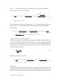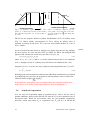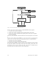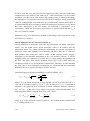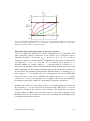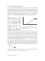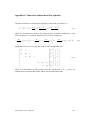
Download Alterra Report1649 - Swap32 Theory description and user manual

SWAP version 3.2. Theory description and user manual
Update 02 : August 2009
Updated items are marked with a red color in the text.
An overview of the updates since the first release of the manual in 2008 is given in
the list below.
Updated item
User
Input
optional
Measured saturated hydraulic conductivity additional to
fitted value in Van Genuchten relation
Soil physical relation in tabulated form functions
optional
Convergency criteria
optional
Switch to suppress the contribution of vertical resistance in mandatory
the phreatic aquifer to the total vertical resistance at the
bottom boundary
Derive Soil cover from a given LAI
no
Input of crop resistance for a wet canopy, completely mandatory
covering the soil (RSW)
Uniformity of fluxes to split ET over Tp and Ep
no
Preferential root water uptake
optional
Time-dependent threshold value for ponding
optional
Adjust the lower boundary of the model discharge layer optional
(lateral drainage)
Introduction of an option to relate the position of the upper optional
boundary of the model discharge layer to the groundwater
level (lateral drainage)
Macropore flow: 1) introduction of user defined resistance optional
of rapid drainage system; 2) specification of one of the
drainage systems number as a “rapid” drainage system; and
3) specification of a ponding threshold
Parameters to relate EC of saturated paste extract to the mandatory
actual salt concentration
Crop growth of grasland according to wofost-approach
optional
Ksat
Page
number
45
θ, K
h, θ,
qbot
45
45
50
Ei
ET
54
58
Tp, Ep
Ta
qpond
qdrain
60
62
163
90
95
qdrain
96
qmp
145
c
163
181
265
Refers to
Variable
Y, ET, q
2
Alterra Report 1649 - update02
SWAP version 3.2. Theory description and user manual
J.G. Kroes
J.C. Van Dam
P. Groenendijk
R.F.A. Hendriks
C.M.J. Jacobs
Alterra Report1649(02) - Swap32 Theory description and user manual.doc
Alterra, Wageningen, 2008
ABSTRACT
Kroes, J.G., J.C. Van Dam, P. Groenendijk, R.F.A. Hendriks, C.M.J. Jacobs, 2008. SWAP
version 3.2. Theory description and user manual. Wageningen, Alterra, Alterra Report1649(02)
- Swap32 Theory description and user manual.doc. 262 pages.; 47 figs.; 12 tables; 39 boxes,
249 refs.
SWAP 3.2 simulates transport of water, solutes and heat in the vadose zone. It describes a
domain from the top of canopy into the groundwater which may be in interaction with a surface
water system. The program has been developed by Alterra and Wageningen University, and is
designed to simulate transport processes at field scale and during whole growing seasons. This
is a new release with special emphasis on numerical stability, macro pore flow, and options for
detailed meteorological input and linkage to other models. This manual describes the
theoretical background, model use, input requirements and output tables.
Keywords: agrohydrology, drainage, evaporation, irrigation, salinization, simulation model,
soil water, solute transport, surface water management, transpiration, vadose zone
ISSN 1566-7197
This report is available in digital format at www.alterra.wur.nl.
A printed version of the report, like all other Alterra publications, is available from Cereales
Publishers in Wageningen (tel: +31 (0) 317 466666). For information about, conditions, prices and
the quickest way of ordering see www.boomblad.nl/rapportenservice
© 2009 Alterra
P.O. Box 47; 6700 AA Wageningen; The Netherlands
Phone: + 31 317 474700; fax: +31 317 419000; e-mail: [email protected]
No part of this publication may be reproduced or published in any form or by any means, or
stored in a database or retrieval system without the written permission of Alterra.
Alterra assumes no liability for any losses resulting from the use of the research results or
recommendations in this report.
4
Alterra Report 1649 - update02
[Alterra Report1649(02) - Swap32 Theory description and user manual.doc/August/2009]
Contents
Preface
9
Summary
11
1
Model overview
1.1 Model domain and processes
1.2 SWAP installation
1.3 Model input
1.4 Model run
1.5 Model output
1.6 Example run: Hupsel catchment
1.7 Reading guide
15
15
16
17
18
21
21
26
2
Soil water flow
2.1 Basic equations
2.2 Soil physical relations
2.3 Modification for near saturation conditions
2.4 Hysteresis
2.5 Frozen soil conditions
2.6 Lower boundary
2.7 Numerical implementation
2.7.1 Richards’ equation
2.7.2 Numerical solution
2.7.3 Numerical implementation of boundary conditions
2.7.3.1 Top boundary condition
2.7.3.2 Bottom boundary condition
2.8 User instructions
2.8.1 General
2.8.2 Bottom boundary conditions
27
27
27
28
29
31
32
34
34
35
38
38
39
43
43
46
3
Evapotranspiration and rainfall interception
3.1 Introduction
3.2 Rainfall interception
3.2.1 Agricultural crops
3.2.2 Forests
3.3 Potential evapotranspiration of uniform surfaces
3.3.1 Penman Monteith method
3.3.2 Reference evapotranspiration and crop factors
3.4 Potential transpiration and evaporation fluxes of partly covered soils
3.5 Actual plant transpiration
3.6 Actual soil evaporation
3.7 User instructions
3.7.1 General information
3.7.2 Weather data
53
53
54
54
55
56
57
59
60
61
62
64
64
66
Alterra Report 1649 - update02
5
3.7.3 Soil data
67
4
Surface runoff, interflow and drainage
69
4.1 Surface runoff
70
4.2 Interflow
71
4.3 Drain discharge
71
4.3.1 Field scale drainage relation according to Hooghoudt and Ernst 75
4.3.2 Field scale drainage relation defined by a tabulated function
78
4.3.3 General aspects of regional scale drainage
79
4.3.4 Regional scale drainage relation defined by a tabulated function 81
4.3.5 Multi-level drainage with fixed resistances and imposed drainage
levels
82
4.3.6 Multi-level drainage with surface water dependent resistances and
simulated drainage levels
83
4.4 Distribution with depth of drainage fluxes
85
4.4.1 Implicit approach of travel times
85
4.4.2 Discharge layers
86
4.5 User instructions
90
4.5.1 Surface runoff
90
4.5.2 Interflow
91
4.5.3 Drainage
91
5
Surface water management
5.1 Surface water balance
5.1.1 Multi-level drainage with imposed surface water levels
5.1.2 Multi-level drainage with simulated surface water levels
5.1.2.1 Fixed weir
5.1.2.2 Soil moisture controlled weir management
5.2 User instructions
5.2.1 Example case
5.2.2 Input instructions
97
97
99
99
99
100
101
101
103
6
Macropore flow
6.1 Concept
6.1.1 Macropore geometry
6.1.1.1 Continuity
6.1.1.2 Persistency
6.1.1.3 Horizontal distribution
6.1.2 Water flow and balance
6.2 Numerical implementation
6.2.1 Macropore geometry
6.2.1.1 Continuity
6.2.1.2 Persistency
6.2.1.3 Horizontal distribution
6.2.2 Water flow and balance
6.3 User instructions
6.3.1 General input parameters
6.3.2 Macropore input parameters
111
111
112
113
116
122
123
130
130
130
132
133
134
137
137
138
6
Alterra Report 1649 - update02
6.3.2.1 Macropore geometry
6.3.2.2 Water flow
138
145
7
Crop growth
7.1 Introduction
7.2 Simple crop module
7.3 Detailed crop module
7.3.1 Phenological development stage
7.3.2 Radiation fluxes above the canopy
7.3.3 Radiation profiles within the canopy
7.3.4 Instantaneous assimilation rates per leaf layer
7.3.5 Daily gross assimilation rate of the canopy
7.3.6 Maintenance respiration
7.3.7 Dry matter partitioning and growth respiration
7.3.8 Senescence
7.3.9 Net growth
7.3.10 Root growth
7.4 User instructions
7.4.1 Simple crop module
7.4.2 Detailed crop module
147
147
147
148
151
152
153
155
156
158
158
160
162
163
163
163
167
8
Solute transport
8.1 Introduction
8.2 Basic equations
8.2.1 Transport processes
8.2.2 Continuity and transport equation
8.3 Boundary conditions
8.4 Crack solute transport
8.5 Residence time in the saturated zone
8.6 User instructions
173
173
174
174
176
178
179
179
181
9
Soil temperature
9.1 Temperature conductance equation
9.2 Numerical solution
9.3 Analytical solution (sinus wave)
9.4 User instructions
185
185
186
189
190
10 Snow and frost
10.1 Snow
10.1.1 Snowfall
10.1.2 Snowpack
10.2 Frost
10.3 User instructions
193
193
193
194
196
199
11 Irrigation
11.1 Fixed irrigation regime
11.2 Scheduled irrigation regime
11.2.1 Timing criteria
11.2.1.1 Allowable daily stress
201
201
201
201
202
Alterra Report 1649 - update02
7
11.2.1.2 Allowable depletion of readily available water
11.2.1.3 Allowable depletion of totally available water
11.2.1.4 Allowable depletion of field capacity water
11.2.1.5 Critical pressure head or moisture content
11.2.1.6 Fixed interval
11.2.1.7 Minimum interval
11.2.2 Depth criteria
11.2.2.1 Back to Field Capacity (+/- specified amount)
11.2.2.2 Fixed irrigation depth
11.2.2.3 Limited depth
11.3 User instructions
202
202
203
203
203
203
203
204
204
204
205
References
209
Appendix 1 Application Penman Monteith method
225
Appendix 2 Derivation of some macropore geometry equations
231
Appendix 3 Examples of description of macropore geometry
235
Appendix 4 Partial derivatives of Fi to pressure heads
237
Appendix 6 Numerical solution heat flow equation
241
Appendix 7 Parameters of soil hydraulic functions: Staring series
245
Appendix 8 Critical pressure head values for root water extraction
247
Appendix 9 Salt tolerance data
249
Appendix 10 Shrinkage characteristic data
251
Appendix 11 Examples of shrinkage characteristics of peat
253
Appendix 12 List of input array lengths
255
Appendix 13 List of main SWAP subroutines
257
Appendix 14 Description of output files *.afo and *.aun
259
Appendix 15 Description of output files *.bfo and *.bun
261
Appendix 16 Crop growth of grassland
265
8
Alterra Report 1649 - update02
Preface
SWAP (Soil-Water-Atmosphere-Plant) is the successor of the agrohydrological
model SWATR (Feddes et al., 1978) and some of its numerous derivatives. Earlier
versions were published as SWATR(E) by Feddes et al. (1978), Belmans et al. (1983)
and Wesseling et al. (1991), as SWACROP by Kabat et al. (1992) and as SWAP93 by
Van den Broek et al. (1994). SWAP2.0 was published by Van Dam et al. (1997) and
Kroes et al. (2001). The latest version was published as SWAP3.0.3 by Kroes and
Van Dam (eds, 2003). Main differences between the current version SWAP 3.2 and
the previous version are:
• Source code was restructured;
• Numerical stability has been largely improved;
• MacroPore flow is operational;
• Detailed rainfall and evapotranspiration data is optional;
• Testing has been strongly intensified;
All reports, together with the SWAP program and examples, are available through the
SWAP-development group and the Internet (www.swap.alterra.nl ).
The general reference to the SWAP model is Van Dam (2000).
The reference to recent advances is Van Dam et al. (2008).
The reference to numerical algorithm is Groenendijk and Kroes (in prep)
The reference to macropore flow is Hendriks et al. (in prep)
Alterra Report 1649 - update02
9
10
Alterra Report 1649 - update02
Summary
SWAP simulates transport of water, solutes and heat in the vadose zone in interaction
with vegetation development. In the vertical direction the model domain reaches from
a plane just above the canopy to a plane in the shallow groundwater. In this zone the
transport processes are predominantly vertical, therefore SWAP is a one-dimensional,
vertically directed model. In the horizontal direction, SWAP’s main focus is the field
scale.
The SWAP model can be downloaded from site www.swap.alterra.nl. The model
input may consist of files for main input, meteorological data, crop growth and
drainage. SWAP employs the TTUTIL library to read the ASCII input files in easy
format. Output is generated in ASCII and binary files. The internet site contains a
large number of SWAP test cases (Chapter 1).
Soil water flow is calculated with the Richards’ equation. The Mualem-Van
Genuchten relations, with a modification near saturation, describe the soil hydraulic
functions. Scaling of main drying and main wetting curves describe hysteresis in the
retention function. The bottom boundary is controlled by head, flux or the relation
between flux and head. SWAP solves the Richards’ equation numerically with an
implicit, backward, finite difference scheme. The Newton-Raphson iterative
procedure ensures mass conservation and rapid convergence (Chapter 2).
For agricultural crops and grassland, SWAP computes the interception following Von
Hoyningen-Hüne and Braden. The interception concept of Gash is available for trees
and forests. The Penman-Monteith equation can be used to calculate the potential
evapotranspiration of uniform surfaces (wet and dry vegetation, bare soil). An
alternative is providing input of reference evapotranspiration in combination with
crop factors. Next the potential transpiration and evaporation fluxes of partly covered
soils are derived, taking into account interception and soil cover. Actual transpiration
depends on the moisture and salinity conditions in the root zone, weighted by the root
density. Actual evaporation depends on the capacity of the soil to transport water to
the soil surface. SWAP uses the soil hydraulic functions and semi-empirical equations
to determine this transport capacity (Chapter 3).
Surface runoff will be calculated when the height of water ponding on the soil surface
exceeds a critical depth. The rate of surface runoff depends on a specified resistance.
Interflow may occur when the groundwater level becomes higher than the interflow
drainage level.
Drainage can be calculated with the Hooghoudt or Ernst equations, with a table
relating drainage flux and groundwater level, or with drainage resistances per
Alterra Report 1649 - update02
11
drainage system. In order to calculate proper residence times of solutes, the drainage
fluxes are vertically distributed according to so-called discharge layers (Chapter 4).
The water balance of the surface water system can be calculated to analyse water
management options. Surface water levels can be imposed, or derived by setting soil
moisture criteria (groundwater level, pressure head, minimum storage) in
combination with a weir (Chapter 5).
Macroporosity can be caused by shrinking and cracking of soil, by plant roots, by soil
fauna, or by tillage operations. The macropore module in SWAP includes infiltration
into macropores at the soil surface, rapid transport in macropores to deeper layers,
lateral infiltration into and exfiltration out of the soil matrix, water storage in
macropores, and rapid drainage to drainage systems. The macropores are divided in a
main bypass domain (network of continuous, horizontal interconnected macropores)
and an internal catchment domain (discontinuous macropores ending at different
depths). The internal catchment domain causes infiltration of macropore water at
different, relatively shallow depth. In addition, the macropores are divided in static
and dynamic volumes. The dynamic volumes depend on shrinkage characteristics
(Chapter 6).
The simple crop module prescribes crop development, independent of external stress
factors. Its main function is to provide a proper upper boundary condition for soil
water movement. In addition, SWAP includes the generic crop growth module
WOFOST. In this module, the absorbed radiation is a function of solar radiation and
crop leaf area. Next the produced carbohydrates (CH2O) are calculated, taking into
account photosynthetic leaf characteristics and possible water and/or salinity stress.
The carbohydrates provide energy for living biomass (maintenance respiration) and
are converted into structural material during which weight is lost as growth
respiration. The material produced is partitioned among roots, leaves, stems and
storage organs, using partioning factors that depend on the crop development stage.
The fraction partioned to the leaves, determines leaf area development and hence the
dynamics of light interception. During crop development a part of the living biomass
dies due to senescence (Chapter 7).
SWAP may simulate transport of salts, pesticides and other solutes that can be
described with basic physical relations: convection, diffusion, dispersion, root uptake,
Freundlich adsorption and first order decomposition. In case of advanced pesticide
transport, including volatilization and kinetic adsorption, SWAP can be used in
combination with PEARL. In case of advanced transport of nitrogen and phosphorus,
SWAP can be used in combination with ANIMO (Chapter 8).
SWAP may simulate soil temperature analytically, using an input sine function at the
soil surface and the soil thermal diffusivity. In the numerical approach, SWAP takes
into account the influence of soil moisture on soil heat capacity and soil thermal
12
Alterra Report 1649 - update02
conductivity. The top boundary condition can be input of air temperatures or soil
surface temperatures (Chapter 9).
The snow module calculates the accumulation and melting of a snowpack when the
air temperature is below a threshold value. The water balance of the snow pack
includes storage, incoming snow and rain and outgoing melting and sublimation.
Melting may occur due to air temperature rise or heat release from rainfall. When a
snowpack is present, the soil temperature top boundary condition is adjusted in order
to account for the insulating effect of the snowpack. In case of frost, reduction factors
can be calculated for the hydraulic conductivity, root water uptake, drainage fluxes
and bottom flux (Chapter 10).
Irrigations with fixed date, depth and quality can be specified as input. In addition,
SWAP can be used to schedule irrigation. Timing criteria include allowable daily
stress, allowable depletion amount and critical pressure head or water content. Depth
criteria include back to field capacity and fixed depth (Chapter 11).
The appendices contain information on the parameters of the soil hydraulic functions,
critical pressure heads for root water extraction, salt tolerance data, shrinkage
characteristic data, numerical solution of water and heat flow, description of binary
output files and list of main SWAP subroutines.
Alterra Report 1649 - update02
13
14
Alterra Report 1649 - update02
1
Model overview
1.1
Model domain and processes
SWAP simulates transport of water, solutes and heat in the vadose zone in interaction with
vegetation development. The model employs the Richards equation including root water
extraction to simulate soil moisture movement in variably saturated soils. Concepts are
added to account for macroporous flow and water repellency. SWAP considers for solute
transport the basic processes convection, dispersion, adsorption and decomposition. For
more extensive studies which for instance include volatilization or nutrient transformations,
SWAP generates soil water fluxes for detailed chemical transport models as PEARL for
pesticides and ANIMO for nutrients. SWAP simulates soil heat flow taking into account
actual heat capacities and thermal conductivities. The generic crop growth module
WOFOST is incorporated to simulate leaf photosynthesis and crop growth. The soil
moisture, heat and solute modules exchange status information each time step to account for
all kind of interactions. Crop growth is affected by the actual soil moisture and salinity
status on a daily basis. An extensive test protocol ensures the numerical code quality of
SWAP.
In the vertical direction the model domain reaches from a plane just above the canopy to a
plane in the shallow groundwater (Fig. 1.1).
Rain
Irrigation
Transport of:
soil water
solutes
soil heat
Transpiration
Evaporation
Interception
Runoff
Snow
Top soil
Sub soil
Groundwater level
Local drainage
flux
Saturated zone
er flux
grondwat
Regional
Aquitard
Second aquifer
Figure 1.1 SWAP model domain and transport processes.
In this zone the transport processes are predominantly vertical, therefore SWAP is a onedimensional, vertical directed model. The flow below the groundwater level may include
Alterra Report 1649 - update02
15
lateral drainage fluxes, provided that these fluxes can be prescribed with analytical drainage
formulas. The model is very flexible with regard to input data at the top and bottom of the
soil column. At the top in general daily weather conditions will suffice. For Nordic
conditions a simple snow storage module has been implemented. In case of more focussed
studies (e.g. runoff or diurnal transpiration fluxes) evapotranspiration and rainfall data can
be specified in more detail. At the bottom various forms of head and flux based conditions
are used.
In the horizontal direction, SWAP’s main focus is the field scale. At this scale most
transport processes can be described in a deterministic way, as a field generally can be
represented by one microclimate, one vegetation type, one soil type, and one drainage
condition. Also many cultivation practices occur at field scale, which means that many
management options apply to this scale. Upscaling from field to regional scale for broader
policy studies is possible with geographical information systems.
The smallest time steps in SWAP are in the order of seconds for fast transport processes
such as intensive rain showers with runoff or flow in macroporous clay soils. These time
steps are automatically increased in periods with less fluctuating flow conditions.
Depending on simulation complexity, computation times for 50 year periods range from 30
to 500 seconds on ordinary personal computers.
1.2
SWAP installation
The SWAP model can be downloaded from Internet site www.swap.alterra.nl. This site
contains also general information on model features, applications and test reports. Various
SWAP versions are available at the Internet site, all running under MS Windows.
SWAP2.0.7.d contains a graphical user interface. This manual applies to SWAP3.2. Only
the most recent SWAP version is supported by the Swap team.
By running the SWAP setup file, a number of folders are created, as depicted in Figure 1.2.
These folders contain:
• Swap executable
• Swap source code
• User manual (in Documents)
• Two examples (Hupsel and CranGras)
• Additional input data:
16
Alterra Report 1649 - update02
Daily weather data of Wageningen
meteorological station of the period 19712000
o Simple crop input data for grass, fodder
maize, potato, sugar beet and winter wheat
o Detailed crop input data for winter wheat,
grain maize, spring barley, rice, sugar
beet, potato, field bean, soy bean, winter
oilseed rape and sunflower
o
After running the setup file, SWAP can be
automatically launched for the example Hupsel.
1.3
Model input
The input data of SWAP are divided over 4 different
file types:
• Main input file (*.swp)
• Meteorological file (*.yyy)
• Crop growth file (*.crp)
• Drainage file (*.dra)
Figure 1.2 Installed folders by
standard SWAP setup file
Box 1.2 provides an overview of the information in these input files. The main input file
and the meteorological data file are always required. Input files of crop growth and drainage
are optional. The extensions of the files are fixed. An exception is the meteorological file,
which has an extension equal to the last 3 digits of the year (e.g. 2008 gives .008). The
names of the input files are free to choose and are specified in the main input file. As listed
in Box 1.1, the main input file contains general information with regard to the simulation,
meteorology, crop rotation scheme, irrigation, soil water flow, heat flow and solute
transport. For meteorological data, commonly a file with daily data is used. In Chapter 3
more detailed input of evapotranspiration and rainfall fluxes will be discussed. The detailed
crop growth input file is required to simulate crop development and biomass assimilation.
As an alternative, the development of crop parameters as leaf area index or rooting depth
can be prescribed in the simple crop growth input file. The drainage input file contains two
sections. The basic drainage section provides input for drainage towards ditches and/or
drains. The extended drainage section provides input for drainage including simulation of
surface water levels.
Alterra Report 1649 - update02
17
SWAP uses the TTUTIL library (Kraalingen & Rappoldt, 2000) for reading input files. Box
1.3 gives an example of a part of the *.swp input file. General rules for the format of input
files are:
• free format with the structure ‘VariableName’ = ‘value’ or in a table with variable
names in the first line (see Box 1.3);
• order of variables is free;
• comment in lines is allowed starting with ‘*’ or ‘!’;
• blank lines are allowed.
In the input files, of each parameter the symbolic name, a description and an identification
is given. The identification between square brackets provides information on:
• range
• unit
• data type (I = Integer, R = Real, Ax = character string of x positions)
For example: [-5000 .. 100 cm, R] means: value between -5000 and +100 with a unit in cm,
given as a Real data type (which means that in the input file a dot should be added).
1.4
Model run
The most common way to run SWAP is by executing a batch file, which refers to the
SWAP executable and the *.swp file. The batch file and the *.swp file need to be present in
the same directory. The *.swp file contains the names and locations of other input files.
Therefore, it is possible to have separate directories with meteorological, crop and drainage
data.
An example of the batch file is given in Box 1.1. In this case SWAP will use Hupsel.swp as
main input file. If no name is specified behind the call ‘Swap.exe’, SWAP will use
Swap.swp as main input file. The pause statement keeps the window box with screen
messages open when runtime warnings or errors might occur.
Box 1.1 Example of batch file to run SWAP with input file Hupsel.swp
c:\Program Files\SWAP\Swap.exe Hupsel.swp
pause
18
Alterra Report 1649 - update02
Box 1.2 Summary of information in input files. Optional files are denoted with #.
Main input file (*.swp)
• General section
- Environment
- Timing of simulation period
- Timing of boundary conditions
- Processes which should be simulated
- Optional output files
• Meteorology section
- Name of file with meteorological data
- Rainfall intensity
• Crop section
- Crop rotation scheme (calendar and files)
- Crop data input file
- Calculated irrigation input file
- Crop emergence and harvest
- Fixed irrigation parameters (Amount and quality
of prescribed irrigation applications)
• Soil water section
- Initial moisture condition
- Ponding
- Soil evaporation
- Vertical discretization of soil profile
- Soil hydraulic functions
- Hysteresis of soil water retention function
- Maximum rooting depth
- Similar media scaling of soil hydraulic functions
- Preferential flow due to soil volumes with
immobile water
- Preferential flow due to macro pores
- Snow and frost
- Numerical solution of Richards' equation
• Lateral drainage section
- (optional) name of file with drainage input data
- (optional) name of file with runon input data
• Bottom boundary section
- (optional) name of file with bottom boundary
conditions
- selection out of 8 options
• Heat flow section
- calculation method
• Solute transport section
- Specify whether simulation includes solute
transport or not
- Top boundary and initial condition
- Diffusion, dispersion, and solute uptake by roots
- Adsorption
- Decomposition
- Transfer between mobile and immobile water
volumes (if present)
- Solute residence in the saturated zone
Alterra Report 1649 - update02
File with daily meteorological data (*.yyy)
- Radiation, temperature, vapour pressure, wind
speed, rainfall and/or reference
evapotranspiration,
- rainfall intensities
File with Detailed crop growth (*.crp) #
• Crop section
- Crop height
- Crop development
- Initial values
- Green surface area
- Assimilation
- Assimilates conversion into biomass
- Maintenance respiration
- Dry matter partitioning
- Death rates
- Crop water use
- Salt stress
- Interception
- Root growth and density distribution
• Calculated Irrigation section
- General
- Irrigation time criteria
- Irrigation depth criteria
File with Simple crop growth (*.crp) #
• Crop section
- Crop development
- Light extinction
- Leaf area index or soil cover fraction
- crop factor or crop height
- rooting depth
- yield response
- soil water extraction by plant roots
- salt stress
- interception
- Root density distribution and root growth
• Calculated Irrigation section
- General
- Irrigation time criteria
- Irrigation depth criteria
File with drainage data (*.dra) #
• Basic drainage section
- Table of drainage flux - groundwater level
- Drainage formula of Hooghoudt or Ernst
- Drainage and infiltration resistances
• Extended drainage section
- Drainage characteristics
- Surface water level of primary and/or secondary
system
- Simulation of surface water level
- Weir characteristics
19
Box 1.3 Example of input according to TTUTIL in main file *.SWP.
* General data
METFIL = 'Wageningen' ! File name of meteorological data without extension .YYY, [A16]
! Extension equals last 3 digits of year number, e.g. 2003 has extension .003
SWETR = 0
! Switch, use reference ET values of meteo file [Y=1, N=0]
* If SWETR = 0, then LAT,ALT and ALTW must have realistic values
LAT
=
52.0
! Latitude of meteo station, [-60..60 degrees, R, North = +]
ALT
=
10.0
! Altitude of meteo station, [-400..3000 m, R]
ALTW
=
2.0
! Altitude of wind speed measurement (10 m is default) [0..99 m, R]
*
* Use of detailed meteorological records (< 1 day)
SWMETDETAIL = 0
! Switch, use detailed meteor. records of both ET and rainfall [Y=1, N=0]
*
* In case of detailed meteorological weather records (SWMETDETAIL = 1):
NMETDETAIL = 10
! Number of weather data records per day, [1..96 -, I]
*
* In case of daily meteorological weather records (SWMETDETAIL = 0):
SWETSINE = 0
! Switch, distribute daily Tp and Ep according to sinus wave [Y=1, N=0]
*
*
SWRAIN = 0
! Switch for use of actual rainfall intensity:
! SWRAIN = 0: Use daily rainfall amounts
! SWRAIN = 1: Use daily rainfall amounts + mean intensity
! SWRAIN = 2: Use daily rainfall amounts + duration
! SWRAIN = 3: Use short time rainfall intensities, as supplied in sep. file
* If SWRAIN = 1, then specify mean rainfall intensity RAINFLUX [0.d0..1000.d0 cm/d, R]
* as function of time TIME [0..366 d, R], maximum 30 records
TIME
RAINFLUX
1.0
2.0
360.0
2.0
* End of table
* If SWRAIN = 3, then specify file name of file with detailed rainfall data
RAINFIL = 'WagRain'
! File name of detailed rainfall data without extension .YYY, [A16]
! Extension equals last 3 digits of year number, e.g. 2003 has extension .003
An alternative to run SWAP is by directly executing Swap.exe. In that case the main input
file should be named Swap.swp, and should be located in the same folder as Swap.exe.
Three types of messages may occur:
• error messages generated by the utility library TTUTIL (Kraalingen & Rappoldt, 2000)
with respect to the format of the input data
• warnings with the advise to adapt the combination of selected options because the
specified combination is not feasible
• fatal errors which stop the simulation
Output files will be generated in the same directory as the main input file. Also the log file
of the most recent simulation run can be found here. The Swap.log file contains a copy of
the *.swp file, possible errors and warnings, and in case of a successful simulation run:
‘Swap simulation okay!’
20
Alterra Report 1649 - update02
1.5
Model output
Output from SWAP is stored in general ASCII files. Some of these files are always
generated, other files are optional output. Box 1.4 provides an overview of the variables that
are printed in each output file. All output files have the same header with the project name,
file content, file name, model version, date of generation, period of calculations and the
depth of the soil profile. The output interval may range from a day to years. Some output
can be generated with time intervals less than a day. We may distinguish output of state
variables, incremental fluxes since the last output time, and cumulative fluxes since a
specified data. The output file with final values of state variables can be used as input for a
subsequent simulation period. This might be useful to derive suitable initial conditions.
In addition to the ASCII files, formatted and unformatted (binary) export files can be
generated with data that cover the entire simulation period. These output files can be used
as input for other models, such as the pesticide and nutrient models like PEARL (Leistra et
al., 2001) and ANIMO (Groenendijk et al., 2005). A description of these files is given in
Appendix 14 Description of output files *.afo and *.aun and Appendix 15 Description of
output files *.bfo and *.bun).
1.6
Example run: Hupsel catchment
The setup file contains the input for a field in the Hupsel catchment in The Netherlands. The
simulation run covers the years 1980-1982. The potential evapotranspiration fluxes are
calculated from daily meteorological measurements. Daily rainfall fluxes are used, as in the
catchment with mild slopes and sandy soils no runoff is expected. The cropping pattern
consists of maize in the summer season of 1980 and 1982. The development of these crops
is prescribed. In the summer season of 1981 potatoes are grown, of which the actual growth
is simulated. On 5 January 1980 a tracer is applied, which leaches in the subsequent years
towards the drains. Initial soil water contents are assumed to be in hydrostatic equilibrium
with a groundwater level at 75 cm depth. The sandy soil profile consists of a top- and
sublayer with thicknesses of 30 and 170 cm, respectively. At the bottom of the soil profile a
layer of boulder clay with low permeability prevents vertical soil water movement.
Therefore at the bottom a zero flux condition is specified. Drainage fluxes are calculated for
subsurface drains at 80 cm depth and with a lateral distance of 11 m. Results are shown in
water balances in Box 1.5 (summary) and Box 1.6 (detail).
Alterra Report 1649 - update02
21
Box 1.4 Summary of information in output files. Optional files are denoted with #.
Short water and solute balance (*.bal)
Final and initial water and solute storage
Water balance components
Solute balance components
Extended water balance (*.blc) #
Final and initial water storage
Water balance components of sub systems
Incremental water balance (*.inc)
Gross rainfall and irrigation
Interception
Runon and runoff
Potential and actual transpiration
Potential and actual evaporation
Net drainage and bottom flux
Cumulative water balance (*.wba)
Gross and net rainfall
Runon and runoff
Potential and actual transpiration
Potential and actual evaporation
Net lateral flux (drainage)
Net bottom flux
Change water storage in profile
Groundwater level
Water balance error
Log file (SWAP.log)
Echo of input (*.swp-file)
Errors and warnings
Cumulative solute balance (*.sba) #
Flux at soil surface
Amount decomposed
Amount taken up by plant roots
Amount in soil profile
Amount in cracks
Flux at soil profile bottom
Drainage flux
Bypass flux from cracks
Amount in defined saturated aquifer
Flux from defined saturated aquifer
Soil temperatures (*.ate) #
Soil temperature of all nodes
Soil profiles (*.vap) #
Profiles of water content, pressure head, solute concentration,
temperature, water flux and solute flux
Irrigation (*.irg) #
Calculated irrigation applications
Detailed crop growth (*.crp)
Development stage
Leaf area index
Crop height
Rooting dept
Cumulative relative transpiration during DVS: 0-2 and 1-2
Cumulative potential and actual weight of dry matter
Cumulative potential and actual weight of storage
22
Simple crop growth (*.crp)
Development stage
Leaf area index
Crop height
Rooting depth
Cumulative relative transpiration
Cumulative relative crop yield
Transpiration stress (*.str)
Potential and actual transpiration
Transpiration reduction due to wet, dry, saline and frost
conditions
Extended drainage components (*.drf) #
Drainage fluxes of each level
Total drainage flux
Net runoff
Rapid drainage
Surface water management 1 (*.swb) #
Groundwater level
Weir target level
Surface water level
Storage in surface water reservoir
Sum of drainage, runoff and rapid drainage
External supply to surface water reservoir
Outflow from surface water reservoir
Surface water management 2 (*.man) #
Weir type
Groundwater level
Pressure head for target level
Total air volume in soil profile
Weir target level
Surface water level and outflow
Number of target level adjustments
Indicator weir overflow
Weir crest level
Snowpack water balance (*.snw) #
Final and initial water storage
Water balance components
Detailed waterbalance Macropores (*.bma) #
Final and initial water storage
Water balance components
Soil physical parameters (soilphysparam.csv)
For each soil layer the relation between: soil water pressure
head h (cm), theta θ (cm3.cm-3), differential capacity C(cm-1),
RelSat Se (-) and hydraulic conductivity K (cm.d-1)
Soil heat conductivity and capacity (heatparam.csv) #
For each soil layer the relation between theta, heatcapacity
and heat conducitivity
Final values of state variables (*.end)
Snow and ponding layer
Soil water pressure heads
Solute concentrations
Soil temperatures
Alterra Report 1649 - update02
Box 1.5 Example of Result.bal file for Hupsel case.
*
*
*
*
*
Project:
File content:
File name:
Model version:
Generated at:
Hupsel
overview of actual water and solute balance components
.\Result.bal
Swap 3.2 (revision 10) (Date 02 May 2008)
05-May-2008 15:57:05
Period
:
Depth soil profile :
Final
:
Initial :
Change
01-Jan-1980 until
200.00 cm
Water storage
72.19 cm
72.07 cm
=============
0.12 cm
31-Dec-1980
Solute storage
0.4570E+02 mg/cm2
0.0000E+00 mg/cm2
=================
0.4570E+02 mg/cm2
Water balance components (cm)
In
=========================
Rain + snow
:
66.01
Runon
:
0.00
Irrigation
:
0.05
Bottom flux
:
0.00
=========================
Sum
:
66.06
Out
============================
Interception
:
4.52
Runoff
:
0.00
Transpiration
:
25.82
Soil evaporation :
14.42
Crack flux
:
0.00
Drainage level 1 :
21.17
============================
Sum
:
65.94
Solute balance components (mg/cm2)
In
=========================
Rain
: 0.0000E+00
Irrigation : 0.5000E+02
Bottom flux : 0.0000E+00
=========================
Sum
: 0.5000E+02
Out
============================
Decomposition : 0.0000E+00
Root uptake
: 0.0000E+00
Cracks
: 0.0000E+00
Drainage
: 0.4300E+01
============================
Sum
: 0.4300E+01
Output is requested at the end of each month for incremental and cumulative fluxes,
and at the end of each year for overviews of the water and solute balance. Box 1.5
shows the water and solute balance components for the year 1980. The rainfall (66.01
cm) is divided over interception (4.52 cm), transpiration (25.82 cm), soil evaporation
(14.42 cm) and drainage (21.17 cm). The soil water storage increases slightly with
0.12 cm. During the experiment a tracer application 500 mg/cm2 has been applied.
After one year, 4.3 mg/cm2 solutes have leached towards the drains, the remaining
amount (45.7 mg/cm2) is still in the soil profile.
Alterra Report 1649 - update02
23
A more detailed overview of the water balance components is given in the Result.blc
file (Box 1.6). In this output file the fluxes are presented between the subdomains
plant, snow, pond layer, soil, and their environment, as depicted in Figure 1.3. Apart
from the in- and outgoing fluxes, of each subdomain also the water storage and
balance is depicted. For instance the ponding layer received 61.49 cm rain and 7.57
cm soil water from the first soil compartment. Of this amount 14.42 cm evaporated
towards the atmosphere, and 54.69 cm infiltrated into the first soil compartment. As
both the initial and final storage of the ponding layer are zero, the storage change is
also zero.
Box 1.6 Example of Result.blc file for Hupsel case.
*
*
*
*
*
Project:
File content:
File name:
Model version:
Generated at:
Hupsel
detailed overview of water balance components (cm)
.\Result.blc
Swap 3.2 (revision 10) (Date 02 May 2008)
05-May-2008 15:57:05
Period
: 01-Jan-1980 until 31-Dec-1980
Depth soil profile : 200.00 cm
=================================================+=================================================
INPUT
| OUTPUT
PLANT
SNOW
POND
SOIL |
PLANT
SNOW
POND
SOIL
=================================================+=================================================
Initially Present
0.00
0.00
72.07 | Finally present
0.00
0.00
72.19
Gross Rainfall
66.01
|
Nett Rainfall
0.00
61.49
| Nett Rainfall
61.49
Gross Irrigation
0.05
|
Nett Irrigation
0.05
| Nett Irrigation
0.05
| Interception
4.52
Snowfall
0.00
|
Snowmelt
0.00
| Snowmelt
0.00
| Sublimation
0.00
| Plant Transpiration
25.82
| Soil Evaporation
14.42
Runon
0.00
| Runoff
0.00
Inundation
0.00
|
Infiltr. Soil Surf.
54.69 | Infiltr. Soil Surf.
54.69
Exfiltr. Soil Surf.
7.57
| Exfiltr. Soil Surf.
7.57
Infiltr. subsurf.
| Drainage
- system 1
0.00 | - system 1
21.17
Upward seepage
0.00 | Downward seepage
0.00
=================================================+=================================================
Sum
66.06
0.00
69.11 126.76 | Sum
66.06
0.00
69.11 126.76
=================================================+=================================================
Storage Change
0.00
0.00
0.12
Balance Deviation
0.00
0.00
0.00
0.00
===================================================================================================
24
Alterra Report 1649 - update02
Precipitation
Gross rainfall
Snowfall
Gross irrigation
Sublimation
Interception
PLANT
Soil evaporation
Plant transpiration
Nett rainfall
Nett irrigation
Melt
SNOW
Runon
Inundation
POND
Runoff
Infiltration/exfiltration
SOIL
surface
water
Drainage/Infiltration
Up/downward seepage
Figure 1.3 Scheme of water fluxes between the subdomains plant, snow, ponding layer, soil
and surface water.
In this case also the cumulative and incremental fluxes are requested at the end of
each month. Box 1.7 shows the incremental water fluxes for the same year 1980. The
actual transpiration rates are close to the potential transpiration rates due to the high
rain amounts in the summer season and the relatively shallow groundwater level. In
May the maize is not yet covering the soil. The solar radiation fluxes are high, which
cause a high potential soil evaporation rate of 11.977 cm/month. Due to the low
rainfall amounts, the top soil becomes dry, and the actual soil evaporation rate is only
1.107 cm/month.
The simulated groundwater levels fluctuate between 71.6 and 112.9 cm depth.
Box 1.7 Example of Result.inc output file for Hupsel case.
*
*
*
*
*
*
Project:
File content:
File name:
Model version:
Generated at:
Date,Day,
31-Jan-1980, 31,
29-Feb-1980, 60,
31-Mar-1980, 91,
30-Apr-1980,121,
31-May-1980,152,
30-Jun-1980,182,
31-Jul-1980,213,
31-Aug-1980,244,
Hupsel
water balance increments (cm/period)
.\Result.inc
Swap 3.2 (revision 10) (Date 02 May 2008)
05-May-2008 15:57:06
Dcum,
31,
60,
91,
121,
152,
182,
213,
244,
Rain,
4.690,
4.650,
5.490,
4.060,
0.930,
6.620,
14.570,
4.640,
Snow,
0.000,
0.000,
0.000,
0.000,
0.000,
0.000,
0.000,
0.000,
Alterra Report 1649 - update02
Irrig, Interc,
0.050,
0.000,
0.000,
0.000,
0.000,
0.000,
0.000,
0.000,
0.000,
0.013,
0.000,
0.796,
0.000,
1.424,
0.000,
1.076,
Runon, Runoff,
0.000,
0.000,
0.000,
0.000,
0.000,
0.000,
0.000,
0.000,
0.000,
0.000,
0.000,
0.000,
0.000,
0.000,
0.000,
0.000,
Tpot,
0.000,
0.000,
0.000,
0.000,
0.068,
3.629,
7.362,
9.502,
Tact,
0.000,
0.000,
0.000,
0.000,
0.068,
3.521,
4.328,
8.895,
Epot,
0.563,
1.642,
3.316,
6.371,
11.977,
5.680,
1.056,
0.757,
Eact, Drainage, QBottom,
0.545,
2.698,
0.000,
1.150,
4.968,
0.000,
1.843,
2.430,
0.000,
2.273,
3.085,
0.000,
1.107,
0.336,
0.000,
2.192,
0.363,
0.000,
1.056,
6.876,
0.000,
0.757,
0.057,
0.000,
25
Gwl
-71.6
-74.7
-67.9
-75.4
-80.4
-81.4
-74.4
-112.9
1.7
Reading guide
In the next chapters we discuss subsequently:
Chapter 2. Soil water flow
Chapter 3. Evapotranspiration and rainfall interception
Chapter 4. Surface runoff, interflow and drainage
Chapter 5. Surface water system
Chapter 6. Macropore flow
Chapter 7. Crop growth
Chapter 8. Solute transport
Chapter 9. Soil heat flow
Chapter 10. Snow and frost
Chapter 11. Irrigation
The first part of each chapter describes the physical relations incorporated in SWAP.
This part also describes implemented numerical procedures, if required to use SWAP
in a proper way. The second part of each chapter describes the model input. If
relevant, suggestions for input are included.
The appendices contain information on:
• Description of the application of the Penman Monteith method
• Description of derivation and examples of macropore equations
• Equations for the partial derivatives of Fi to pressure heads
• Equations for the implicit linearization of hydraulic conductivities
• Equations for the numerical solution of heat flow
• Tables with soil hydraulic functions: Staring Series 2001
• Tables with critical pressure heads for root water extraction
• Tables with salt tolerance data
• Tables with shrinkage characteristic data
• Tables with shrinkage characteristic data for peat soils
• List of subroutines
• List of fixed ranges of array lengths
• Listing of formatted and unformatted binary output files
• Description of WOFOST crop growth routine for grassland
26
Alterra Report 1649 - update02
2
Soil water flow
2.1
Basic equations
Gradients of the soil water potential induce soil water movement. Darcy's equation is
commonly used to quantify these soil water fluxes. For one-dimensional vertical
flow, Darcy's equation can be written as:
q = − K ( h)
∂ (h + z )
∂z
(2.1)
where q is soil water flux density (positive upward) (cm d-1), K(h) is hydraulic
conductivity (cm d-1), h is soil water pressure head (cm) and z is the vertical
coordinate (cm), taken positively upward.
Water balance considerations of an infinitely small soil volume result in the
continuity equation for soil water:
∂θ
∂q
= − − S a ( h) − S d ( h) − S m ( h)
∂t
∂z
(2.2)
where θ is volumetric water content (cm3 cm-3), t is time (d), S a (h) is soil water
extraction rate by plant roots (cm3 cm-3 d-1), S d (h) is the extraction rate by drain
discharge in the saturated zone (d-1) and S m (h) is the exchange rate with macro pores
(d-1).
Combination of Eqs. [2.1] and [2.2] provides the general water flow equation in
variably saturated soils, known as the Richards' equation:

 ∂h 
∂  K (h) + 1
∂θ
 ∂z 
− S a ( h) − S d ( h) − S m ( h)
= 
∂z
∂t
(2.3)
SWAP applies Richards' equation integrally for the unsaturated-saturated zone,
including possible transient and perched groundwater levels. SWAP solves Eq. [2.3]
numerically, using known relations between θ, h and K.
2.2
Soil physical relations
The Mualem-Van Genuchten function (Van Genuchten, 1980) which has been used in
numerous studies and forms the basis of several national and international data-bases
(e.g. Carsel and Parrish, 1988; Yates et al., 1992; Leij et al., 1996; Wösten et al.,
2001) has been implemented in SWAP. The analytical θ(h) function proposed by Van
Genuchten (1980) reads:
(
θ = θ res + (θ sat − θ res ) 1 + α h
Alterra Report 1649 - update02
)
n −m
(2.4)
27
where θsat is the saturated water content (cm3 cm-3), θres is the residual water content
in the very dry range (cm3 cm-3) and α (cm-1), n (-) and m (-) are empirical shape
factors. Without loosing much flexibility, m can be taken equal to :
m = 1−
1
n
(2.5)
Using the above θ(h) relation and applying the theory on unsaturated hydraulic
conductivity by Mualem (1976), the following K(θ) function results:
1 m
 

m
=
K K sat Se 1 − 1 − Se  
 
 
2
λ
(2.6)
where Ksat is the saturated conductivity (cm d-1), λ is a shape parameter (-) depending
on ∂K/∂h, and Se is the relative saturation defined as:
Se =
θ − θ res
θsat − θ res
(2.7)
The numerical solution to the Richards’ equation requires an approximation of the
differential water capacity C (cm-1). An expression is obtained by taking the
derivative of θ to h:
C=
(
∂θ
n −1
n
= α m n αh (θ sat − θ res ) 1 + αh
∂h
)
− ( m +1)
(2.8)
A numerical approach to Eq. [2.3] yielding a steady-state solution requires an implicit
treatment of the hydraulic conductivity. This implies the use of the derivative of the
hydraulic conductivity to the pressure heads. Expressions are given in 0.
2.3
Modification for near saturation conditions
A modification to the Mualem-Van Genuchten function (Schaap and Van Genuchten,
2006) has been implemented in SWAP. The modification is based on the introduction
of a small minimum capillary height he , causing a minor shift in the retention curve
(Vogel et al. 2001). We follow Ippisch et al. (2006) by defining the relative water
content as:
[
n
1
1 + αh

Se =  Sc

1
]
−m
h < he
h ≥ he
(2.9)
where S c is the relative saturation at the cut-off point he in the classical Van
Genuchten model, given by:
[
S c = 1 + αhe
]
n −m
(2.10)
The hydraulic conductivity is then given by:
28
Alterra Report 1649 - update02
2

1
m 

 K (S )λ 1 − (1 − (S e S c ) m ) 
K =  sat e 
1
m 
 1 − (1 − (S c ) m ) 


K sat
Se < 1
(2.11)
Se ≥ 1
This model reduces to Eq. [2.6] for he = 0. We refer to Vogel et al. (2001), Schaap
and Van Genuchten (2006) and Ippisch et al. (2006) for a detailed discussion of the
above equations. They showed that the modification affects the shape of the retention
curve only minimally relative to the original function. However, the effects on the
unsaturated hydraulic conductivity of fine-textured soils can be significant.
To prevent for numerical instabilities of the solution scheme the soil moisture
retention curve between 1.05 and 0.95 times the he-value is approached by a cubic
spline for which the parameters are chosen as such that the continuity of both the soil
moisture retention curve and the differential moisture capacity function is preserved.
2.4
Hysteresis
Soil water pressure head h
Hysteresis refers to non-uniqueness of the θ(h) relation and is caused by variations of
the pore diameter (inkbottle effect), differences in radii of advancing and receding
meniscus, entrapped air, thermal gradients and swelling/shrinking processes (Hillel,
1980; Feddes et al., 1988). Gradual desorption of an initially saturated soil sample
gives the main drying curve, while slow absorption of an initially dry sample results
in the main wetting curve. In the field partly wetting and drying occurs in numerous
cycles, resulting in so-called drying and wetting scanning curves lying between the
main drying and the main wetting curves (Fig. 2.1).
Scanning drying curves
Scanning wetting curve
Main drying curve
Main wetting curve
0
0
Volumetric water content q
Figure 2.1 Water retention function with hysteresis, showing the
main wetting, main drying and scanning curves.
Alterra Report 1649 - update02
29
In simulation practice, often only the main drying curve is used to describe the θ(h)
relation. This is mainly due to the time and costs involved in measurement of the
complete θ(h) relationship, including the main wetting, the main drying and the scanning
curves, especially in the dry range. For instance, a generally applied soil hydraulic data
base in The Netherlands, known as the Staring series (Wösten et al., 1994), contains only
θ(h) data of the main drying curve. Nevertheless, it is obvious that the simulation of
infiltration events with the main drying curve can be inaccurate. The scaling method of
Scott et al. (1983), who derived scanning curves by rescaling the main wetting or the
main drying curve to the actual water content, has been implemented into SWAP.
The main drying and main wetting curve are described analytically with the Mualemvan Genuchten parameters (α, n, θres, θsat, Ksat, and λ). Some of the parameters
describing the main wetting and main drying curve are related. We assume θres and
θsat to be equal for both curves. Usually the K(θ) function shows only minor
hysteresis effects, which can be achieved by choosing for the main wetting and main
drying curve a common value for n. Ultimately the two curves only differ in the
parameter α, as depicted in Fig.2.1. The scanning curves are derived by linear scaling
of either the main wetting or main drying curve, such that the scanning curve includes
the current θ-h combination and approaches the main wetting curve in case of a
wetting scanning curve and the main drying curve in case of a drying scanning curve.
The scaling principle in case of a drying scanning curve is depicted in Fig.2.2A.
Based on its wetting and drying history, at a certain time and depth the soil shows an
actual water content θact at the soil water pressure head hact. The valid drying scanning
curve should pass through the point (θact, hact), and approach the main drying curve at
smaller water contents.
A
Soil water pressure head h
Main wetting curve (αwet, n, qres, qsat)
Main drying curve (αdry, n, qres,
qsat)
Drying scanning curve (αdry, n, qres,
qsat*)
qmd
hact
Current status
Soil water pressure head h
B
Main wetting curve (αwet, n, qres, qsat)
Main drying curve (αdry, n, qres,
qsat)
Current status
hact
Wetting scanning curve
(αwet, n, qres*, qsat)
qmw
0
0
qres
qact
qsat*
qsat
0
Water content q
0
qres
qres*
qact
qsat
Water content q
Figure 2.2 (A) Linear scaling of the main drying water retention curve in order to derive a drying
scanning curve; (B) Linear scaling of the main wetting water retention curve in order to derive a
drying wetting curve.
30
Alterra Report 1649 - update02
We may define θmd as the water content of the main drying curve at hact, and θsat* as
the saturated water content of the drying scanning curve. Linear scaling of the main
drying curve with respect to the vertical axis θ = θres gives (Fig.2.2A):
*
θsat
− θ res θ act − θ res
=
θsat −θ res θ md −θ res
*
⇒ θsat
=θ res + (θsat −θ res )
θ act − θ res
θ md −θ res
(2.12)
The only unknown in Eq. [2.13] is θsat*, which can be directly solved. The drying
scanning curve is described accordingly with the parameters (αdry, n, θres, θsat*). As long
as the soil keeps drying, this drying scanning curve is valid.
The opposite occurs when the soil gets wetter. Again we start from the arbitrary
actual water content θact at the soil water pressure head hact, and now define θmw as the
water content of the main wetting curve at hact, and θres* as the residual water content
of the wetting scanning curve. Linear scaling of the main wetting curve with respect
to the vertical axis θ = θsat gives (Fig.2.2B):
*
θsat − θ res
θ −θ
= sat act
θsat −θ res θsat −θ mw
*
⇒ θ res
=θsat − (θsat −θ res )
θsat − θ act
θsat −θ mw
(2.13)
From Eq.[2.14], θres* can be directly solved. The wetting scanning curve is accordingly
described with the parameters (αwet, n, θres*, θsat), and is valid as long as the soil keeps
wetting. As the wetting-drying history is different at each soil depth, each node may
show a different scanning curve. The unique K(θ) relation of a soil layer always follows
from the parameter set (n, θres, θsat, Ksat, λ) according to Eq. [2.6].
2.5
Frozen soil conditions
Impacts of frozen soil moisture on soil water flow can optionally be described by a
reduction of the hydraulic conductivity:
K * = K min + ( K − K min ) ⋅ max(0, min( 1,
T − T2
))
T1 − T2
(2.14)
where K* is the adjusted hydraulic conductivity (cm d-1), T is the soil temperature
(oC), T1 and T2 (oC) are the threshold values bounding the linear reduction and K min
is a minimum value of the hydraulic conductivity (cm d-1) which holds for
temperatures less than T2.
Alterra Report 1649 - update02
31
2.6
Lower boundary
The bottom boundary of the one-dimensional SWAP is either in the unsaturated zone
or in the upper part of the saturated zone where the transition takes place to threedimensional groundwater flow. The lower boundary conditions in SWAP can be
specified, depending on the application and the relevant spatial scale.
Three general types and some special cases of lower boundary conditions are
distinguished:
1) The Dirichlet condition
The head controlled boundary is often referred as to the Dirichlet condition and
involves the imposing of a pressure head hbot at the lower boundary. A special case
involves the use of a recorded groundwater elevation. The pressure head at the
groundwater elevation φ avg is defined as h=0. This yields a linear relation between
the pressure heads at the grid points above and below φ avg :
hi +1 = −hi
φ avg − z i +1
z i − φ avg
(2.15)
2) The Neumann condition
The flux is often referred as to the Neumann condition and involves prescribing a
flux qbot at the bottom. Since the model employs an explicit linearization scheme,
the flux - groundwater level relations are treated as a Neumann condition, where
the actual flux is calculated from the groundwater level of the previous time step.
The relation between flux and groundwater level can be obtained from regional
groundwater flow models (e.g. Van Bakel, 1986). Some special options are
available to define qbot:
- A zero bottom flux may be applied when an impervious layer exists at the
bottom of the profile.
- Impose a time series of qbot
- Calculate qbot at the start of a time step as a function of the groundwater level
φavg of the previous timestep, either by interpolation in a tabulated function or
by using an exponential function, defined as:
(
q bot = a bot exp − bbot φavg
)
(2.16)
where abot (cm d-1) and bbot (cm-1) are empirical coefficients.
32
Alterra Report 1649 - update02
-
Calculate qbot at the start of a time step as a function of the groundwater level
φavg of the previous timestep, the hydraulic head in a semi-confined aquifer
φaquif (cm), and the resistance of the semi-confining layer c1 (d), according to:
qbot =
φaquif − φavg
n
c1 +
∑
i =igwl
∆zi
k sat ,i
(2.17)
The flow resistance in the saturated zone between the groundwater level and
the lower boundary has been accounted for by summation of the flow
resistances
∆zi
in this zone. Some options for defining φaquif are available.
k sat ,i
3) The Cauchy condition
The flux q at the lower boundary is defined as a function of the prevailing pressure
head. This condition can be used when unsaturated flow models are combined
with models for regional groundwater flow and when an implicit handling of qbot
in the iterative computation scheme is required. The flux through the bottom
boundary is defined by the difference of the hydraulic head (h+z) and the hydraulic
head φ (cm) of the regional groundwater outside the flow domain described by the
model, divided by a flow resistance c (d).
qbot =
[h + z ]z =bot − ϕ
c
(2.18)
4) Special cases
Two special cases involve the option to define a seepage face at the lower
boundary and to define free drainage. The seepage face is meant to simulate
moisture flow in a lysimeter which is composed of a combination the head
controlled condition and the zero flux controlled condition.
hz =bot < 0 → qbot = 0
 ∂ (h + z ) 
hz =bot </ 0 → qbot = − K n 

 ∂z  z =bot
(2.19)
The free drainage results from the assumption that the hydraulic head gradient
equals the elevation head gradient, thus: so that the magnitude of qbot equals the
hydraulic conductivity of the lowest compartment:
 ∂ (h + z ) 
= 1 → qbot = − K n
 ∂z 

 z =bot
Alterra Report 1649 - update02
(2.20)
33
During frost conditions, qbot will be modified according to
qbot = fT ( z ) qbot
(2.21)
but can be reduced even to a lower value in case of the presence of frozen layers (see
Chapter 10).
2.7
Numerical implementation
Accurate numerical solution of Richards' partial differential equation is difficult due
to its hyperbolic nature, the strong non-linearity of the soil hydraulic functions and
the rapid changing boundary conditions near the soil surface. Calculated soil water
fluxes can be significantly affected by the structure of the numerical scheme, the
applied time and space discretizations, and the procedure for the top boundary
condition (Van Genuchten, 1982; Milly, 1985; Celia et al., 1990; Warrick, 1991;
Zaidel and Russo, 1992). The numerical scheme chosen in SWAP solves the onedimensional Richards' equation with an accurate mass balance and converges rapidly.
This scheme in combination with the top boundary procedure has been shown to
handle rapid soil water movement during infiltration in dry soils accurately. At the
same time the scheme is computationally efficient (Van Dam and Feddes, 2000).
2.7.1 Richards’ equation
The current numerical scheme of SWAP to solve Richards’ equation is the implicit,
backward, finite difference scheme with explicit linearization of hydraulic
conductivities as described by Haverkamp et al. (1977) and Belmans et al. (1983), but
with the following adaptations:
• The numerical scheme applies to both the unsaturated and saturated zone and
the flow equations are solved in both zones simultaneously.
•
The water storage term
C
•
∂θ
is evaluated instead of using an approximation for
∂t
∂h
where C is the water capacity (cm-1).
∂t
There are several options for calculating the internodal conductivity.
The implicit, backward, finite difference scheme of Eq. [2.23] with explicit
linearization, yields the following discretization of Richards' equation:
34
Alterra Report 1649 - update02
θ i j +1 − θ i j
=
∆t j
−
1
∆zi
S aj, i
 j + κ hi j−+11 − hi j +1

hi j +1 − hi j++11
+ K i j−+½κ − K i j++½κ
− K i j++½κ 
 K i −½
½ (∆zi −1 + ∆zi )
½ (∆zi + ∆zi +1 )


−
S dj , i
−
(2.22)
S mj +, i1
where ∆t j = t j+1 - t j and ∆zi is compartment thickness. The sink terms representing
the root extraction Sa and the flow to drains Sd are evaluated at the old time level j
(explicit linearization). The macro pore exchange rate Sm is evaluated at the new time
level j+1 and the internodal conductivity K i −j +½κ can be evaluated at the old time level j
( κ = 0 ) or at the new time level j+1 ( κ = 1 ). The internodal conductivity K i j−+½κ can
be calculated as:
Arithmic mean:
(
K i j−+½κ = ½ K i j−+1κ + K i j +κ
)
(2.23)
j +κ
i −1
∆z i −1 K
+ ∆z i K i
∆z i −1 + ∆z i
Weighted arithmic mean:
K i −j +½κ =
Geometric mean:
K i j−+½κ = K i j−+1κ
Weighted geometric mean:
K i j−+½
j +κ
( ) (K κ )
κ
(K κ )
= (K κ )
½
j+
i −1
j+
½
i
∆z i −1
∆z i −1 + ∆z i
j+
i
∆z i
∆z i −1 + ∆z i
(2.24)
(2.25)
(2.26)
Starting in the saturated zone, the groundwater table is simply found at h = 0. Also
perched water tables may occur above dense layers in the soil profile. Since the
SWAP model attempts to describe a wide range of layered soil types combined with
different types of boundary conditions, the nodal distance is made variable and should
be specified by the user. Calculations using a non-weighted arithmic mean for the
internodal conductivity show that for accurate infiltration and evaporation
simulations, the nodal distance should be in the order of centimetres near the soil
surface (Van Dam and Feddes, 2000).
2.7.2 Numerical solution
The discrete form of the Richard’s equation is solved iteratively using the pressure
heads as state variables. Taylor-expansion of the new moisture fraction at a new
iteration level with respect to the moisture fraction at the preceding iteration step is
defined by:
θ i j +1, p +1 (hi j +1 ) ≈ θ i j +1, p (hi j +1, p ) + (hi j +1, p +1 − hi j +1, p )
∂θ i j +1, p
∂hi j +1, p
+ +
(2.27)
Ignoring the second and higher order terms of the Taylor series yields an expression
which can substitute the moisture fraction variable at the new time-level. The first
order derivate of the moisture fraction to the pressure head is identical to the water
capacity C j +1, p . In fact the basis (first order approximation of the new moisture
Alterra Report 1649 - update02
35
fraction) of the method proposed by Celia et al. (1990) complies with the assumptions
made in the Newton-Raphson iteration procedure. An improvement to this method is
made by defining Fi based on the closure term of the water balance as a function of
hi j +1 :
Fi =
+
∆zi
∆t
j
(θ
j +1, p
i
K i j++½κ ,κp
)
− θ i j − K i j−+½κ ,κ p
hi j−+11, p − hi j +1, p
− K i j−+½κ ,κ p
½ (∆zi −1 + ∆zi )
(2.28)
hi j +1, p − hi j++11, p
+ K i j++½κ ,κ p + ∆zi S aj,+i κ , p + ∆zi S dj ,i + ∆zi S mj +,i1, p
½ (∆zi + ∆zi +1 )
where the superscript p+1 points to the solution of iteration round p. This discrete
form of the Richards’ equation allows for a straightforward evaluation of the storage
term and is flexible with the respect to adding of hi j +1 -dependent source and sinkterms. Solving the set of non-linear equations numerically implies root finding of the
function Fi ≈ 0 for i=1..N. The Newton Raphson-iteration scheme for the set of
equations is written as follows:
 ∂F1
 j +1, p
 ∂h1

 h1j +1, p +1   h1j +1, p   ∂F2

 
 ∂h j +1, p

     1

 j +1, p +1   j +1, p   0
 hi
 =  hi
−




  
 j +1, p +1   j +1, p   0
 hn
  hn
 

 0


∂F1
∂h2j +1, p
∂F2
∂h2j +1, p
∂Fi
∂hi j−+11, p
0
0
0

0
0
∂Fi
∂Fi
0
0

∂hi j++11, p
∂Fn −1
0
0
∂Fn
∂hi
j +1, p
∂hnj−+11, p
∂hnj−+11, p
∂Fn −1
∂hnj +1, p
∂Fn
∂hnj +1, p















−1
 F1 
 
  
F 
 i
  
 
 Fn 
(2.29)
The starting values are the results of the previous iteration round, indicated by the
superscript p. The solution of the second part of the right hand side is found by
solving a tri-diagonal system of equations which can be solved efficiently (Press et
al., 1989). The coefficients of the Jacobian are listed in 0. The contribution of the
partial derivative of the macro-pore exchange to the pressure head (
∂S mj +,i1, p
∂hi j +1, p
) is discussed
in Chapter 6. If the option to treat the hydraulic conductivities implicitly is used (κ=1),
the contribution of the partial derivates of the internodal conductivity relation to the
pressure head should also accounted. Expressions for these terms are given in 0.
Newton’s method for solving nonlinear equations might wander off into the wild blue
yonder if the initial guess is not sufficiently close to the root.
36
Alterra Report 1649 - update02
F(hij,p)
hij,p+1
hij,p
Figure 2.3 Influence of initial estimate on an intermediate solution of a first order
approximation based root finding procedure.
The solution to the second part of the right hand side of Eq. [2.30] is referred to as the
Newton-step ∆hi j +1, p (Eq. [2.31]).
 h1j +1, p +1   h1j +1, p 
 ∆h1j +1, p 

 



 
   
  
 j +1, p +1   j +1, p 
 j +1, p 
 hi
 =  hi
 + λ  ∆hi

 
   
  
 j +1, p +1   j +1, p 
 j +1, p 
 hn
  hn

 ∆hn

(2.30)
We always first try the full Newton step and we check at each iteration that the
n
proposed step reduces ½∑ Fi 2 . If not, we backtrack along the Newton direction until
i =1
we have an acceptable step. The aim is to find λ which results in a decrease of
∑ [Fi (hij +1, p + λ ∆hij +1, p )]
n
½
2
. The first estimate of λ amounts to 1. If it is decided that a
i =1
second estimate is needed, λ is set to 1/3. The third estimate amounts to 1/9.
Thereafter, no further reduction of λ is applied but a new Newton -iteration step is
performed.
In SWAP the main convergence criterium in the unsaturated zone is based on the
water closure term of the water balance F. If Fi is less than a user defined criterion
for all compartments, it is decided that the iteration cycle has resulted into a
sufficiently accurate solution.
Alterra Report 1649 - update02
37
2.7.3 Numerical implementation of boundary conditions
2.7.3.1 Top boundary condition
Appropriate criteria for the procedure with respect to the top boundary condition are
important for accurate simulation of rapidly changing soil water fluxes near the soil
surface. This is for instance the case with infiltration/runoff events during intensive
rain showers or when the soil occasionally gets flooded in areas with shallow
groundwater tables. At moderate weather and soil wetness conditions the soil top
boundary condition will be flux-controlled. In either very wet or very dry conditions
the prevailing water pressure head at the soil surface starts to govern the boundary
condition.

 hi j−+11, p − hi j +1, p
+ 1 is

 ½ (∆zi −1 + ∆zi ) 
In case of a Flux controlled top boundary the term − K i j−+½κ ,κ p 
replaced by the flux through the soil surface qtop (cm d −1 ) which yields the following
expression:
F1 =
∆z1
∆t j
(θ
j +1
− θ1j
1
)+ q
top
+ K1j½+κ
h1j +1 − h2j +1
+ K1j½+κ + ∆z1S aj,+1κ + ∆z1S dj ,1 + ∆z1S mj +,11 (2.31)
½ (∆z1 + ∆z2 )
where qtop is calculated from external driving factors as net precipitation (qprec),
irrigation (qirri), melt of a snow pack (qmelt) runon originating from adjacent fields
(qrunon) and inundation from adjacent water courses (qinun)
qtop = −q prec − qirri − q melt − q runon − qinun
(2.32)

 hi j−+11, p − hi j +1, p
+ 1 is

 ½ (∆zi −1 + ∆zi ) 
In case of a Head controlled top boundary the term − K i j−+½κ ,κ p 
 h0j +1 − h1j +1
replaced by − K½j +1 
 ½ (∆z1 )

+ 1 , where h0j +1 is the pressure head at the soil surface


at the new time level. The internodal conductivity K½j +1 is always treated implicitly.
Within each iteration round and also within each backtracking sub-cycle it is tested
 qtop
whether the combination of qtop and h1j +1 would lead to h1j +1 − ½(∆z1 )

K ½j +1

+ 1 > 0 . In


such a case it is decided that the head boundary condition holds and the water balance
of the so-called ponding layer is calculated which includes the surface runoff flux and
38
Alterra Report 1649 - update02
the ponding depth at time level j+1. The value of
h0j +1 is
set to the ponding depth at
time level j+1. The water balance of the ponding layer reads as:

 h j +1 − h1j +1
h0j +1 − h0j
= − K ½j +1  0
+ 1 + q prec + qirri + qmelt + qrunon + qinun − qe , pond − qrunoff − I ru
∆t

 ½ (∆z1 )
(2.33)
Where Iru is the runoff into the macropores (section 6.1.2).
The surface runoff flux qrunoff is defined as a function of the ponding height:
h0j +1 ≤ h0,threshold
qrunoff = 0
h0j +1 > h0,threshold
qrunoff = α h0j +1 − h0,threshold
(
)
β
(2.34)
Where α and β are coefficients of the surface runoff equation employed by the
SWAP model (see Section 4.1). Substitution of surface runoff expression into water
balance equation for the ponding layer yields the relation which is solved in the
iteration procedure:
 1
β
K j +1 
h0j +1  + ½  + α h0j +1 − h0,threshold =
 ∆t ½ (∆z1 ) 
(
)
h0j
K j +1
+ ½ h1j +1 − K½j +1 + q prec + qmelt + qrunon − qe , pond − I ru
∆t ½ (∆z1 )
(2.35)
which is solved in the iteration procedure.
2.7.3.2 Bottom boundary condition
The SWAP model provides a number of options to describe the relation between
saturated shallow soil layers with deep groundwater (see Chapter 5). Beside handling
the flux controlled boundary condition and head controlled boundary condition, the
model has additional capabilities to combine these basic types of conditions.
Additional options comprise the handling of:
• Predefined groundwater levels
• Cauchy relation for the bottom boundary
• Free drainage
• Free outflow
Alterra Report 1649 - update02
39
Flux controlled bottom boundary

 hi j +1, p − hi j++11, p
+ 1 -term in Eq. [2.29] is replaced by − qbot , which

 ½ (∆zi + ∆zi +1 ) 
For i=n, the K i j++½κ ,κp 
yields:
Fn =
∆z n
∆t j
(θ
j +1
n
(
)
)
 hnj−+11 − hnj +1

− θ nj − K nj−+½κ 
+ 1 − qbot + ∆z n S aj,+nκ + S dj , n + S mj +, n1 (2.36)
 ½ (∆z

n −1 + ∆z n )


Beside the flux boundary condition, the SWAP model has options to handle groundwater
level dependent bottom fluxes. The flux can be formulated as an exponential function of
groundwater level, or as the difference between groundwater level and hydraulic head in
deep groundwater outside the flow domain divided by a flow resistance. Such a flux is
calculated explicitly at the start of the current time step and is treated as a flux condition
in the numerical scheme.
Head controlled bottom boundary
For i=n, ∆zi +1 is set to zero and hi +j +11, p = hbot , which leads to the following expression:
Fn =
(
)

 h j +1 − h j +1

 h j +1 − hbot
∆z n j +1
θ n − θ nj − K nj−+½κ  n −1 n
+ 1
+ 1 + K nj++½κ  n
j
 ½ (∆z n −1 + ∆z n ) 
∆t

 ½ ∆z n


+
(
∆z n S aj,+nκ
+
+
S dj , n
S mj +, n1
)
(2.37)
Predefined groundwater levels
First, the lowest partially unsaturated compartment is searched for and is called n*.
The set of n* non-linear equations for F(h) is then solved for the unsaturated
compartments. The bottom boundary condition for this set of equations is defined by:
Fn* =
∆z n*
∆t
(
θ nj*+1
j
(
− θ j*
n
+ ∆z n S j +κ* + S j
a ,n
d , n*
)−
 h j*+1 − h j*+1
j +κ 
n −1
n
K *
n −½  ½ ( ∆z
+
∆z n* )
*
n −1

+ S j +1*
m ,n
)


 h j*+1 − h j*+1
j +κ 

n
n +1
+1 + K *
+ 1
n +½  ½ ( ∆z + ∆z

)  (2.38)
n*
n* +1



The groundwater level is situated between the nodal points n* and n*+1. The pressure
head of nodal point n*+1 is approximated hnj*+1 by:
hnj*++11 = −hnj*+1
40
gwl − zn* +1
zn* − gwl
(2.39)
Alterra Report 1649 - update02
where
zn*
is the height of the node in compartment n* and gwl is the groundwater
level. Substitution into Eq. [2.30] yields:
Fn* =
j
(θ
(
a ,n
∆z n*
∆t
j +1
n*
−θ
j
n*
+ ∆z n S j +κ* + S j
d ,n*
)


 
 h j +1  z n* − z n* +1  
*


 n  z * − gwl  
 n
 + 1
− K j*+κ 
+ 1 + K j*+κ 
n −½  ½ ( ∆z
n
+

½
+ ∆z n* )
 ½ (∆z n* + ∆z n* +1 )

n* −1








h j*+1
n −1
+ S j +1*
m,n
− h j*+1
n
(2.40)
)
After iteratively solving the set of equations for i ≤ n*, the pressure head profile of the
compartments i > n* can be calculated from the pressure head of the two adjacent
upward nodes.
j +κ
j +κ
 K j +κ ( ∆z i + ∆z i +1 ) 
 − h j +1 K i −½ (∆z i + ∆z i +1 ) + ½ (∆z i + ∆z i +1 )(1 − K i −½ )
hi +j +11 = hi j +1 1 + i −j +½κ
 K
 i −1 K j +κ (∆z + ∆z )
K i j++½κ
i −1
i
i +½ ( ∆z i −1 + ∆z i ) 
i +½

(2.41)
½ (∆z i + ∆z i +1 )  ∆z i
j
j +κ
j
j +1 
+
 j θ sat ,i − θ i + ∆z i S a ,i + S d ,i + S m,i 
K i j++½κ

 ∆t
(
)
(
)
Cauchy relation for the bottom boundary
The flux through the bottom boundary is defined by the difference the hydraulic head
at the lower boundary and the hydraulic head φ (cm) of the regional groundwater
specified by the user, divided by a flow resistance c (d). The hydraulic head at the
lower boundary is approximated by the pressure head of the lowest nodal point plus
the elevation head of node n.
qbot =
hnj +1 + z n − ϕ
½ ∆z n
+c
K nj++½κ
(2.42)
Substitution into Eq. [2.30] yields:
(θ
∆t
+ ∆z (S
Fn =
∆z n
j
n
j +1
n
j +κ
a ,n
)

 hnj−+11 − hnj +1
h j +1 − (ϕ − z n )
− θ nj − K nj−+½κ 
+ 1 + K nj++½κ n

 ½ (∆z n−1 + ∆z n )
½ ∆z n + cK nj++½κ


+ S dj ,n + S mj +,n1
)
(2.43)
Seepage face
The seepage face option is used to simulate the soil moisture flow in a lysimeter with
an open outlet at the bottom. No outflow occurs when the bottom soil layer is still
unsaturated. Since the flow resistance of the outlet is negligible small, no positive
Alterra Report 1649 - update02
41
pressure head values will be build up at the bottom when the soil water percolates at
the bottom. Within the iteration cycle for solving the numerical expression of the
Richards’ equation, it is checked whether the flux or the head controlled boundary
condition prevails. When hnj +1 + ½ ∆z n < 0 the bottom flux qbot is set to zero, but when
hnj +1 + ½ ∆z n tends to take values larger than zero, the pressure at the bottom is set to
zero ( hbot = 0 ). The numerical implementation is as follows:
hnj +1 + ½ ∆z n < 0 →
(
+
Fn =
hnj +1
)
j +1
j +1


∆z n j +1
j + κ  hn −1 − hn
j
K
θ
θ
−
−
+ 1
n
n
n −½ 
j

∆t
 ½ (∆z n −1 + ∆z n ) 
Fn =
+ ½ ∆z n </ 0 →
(
∆z n S aj,+nκ
(
+
S dj , n
+
S mj +, n1
(2.44)
)
)
j +1
j +1


∆z n j +1
j + κ  hn −1 − hn
j
K
−
−
+ 1
θ
θ
n
n
½
n
−
j


∆t
 ½ (∆z n −1 + ∆z n ) 
+
(

hnj +1
+ 1 + ∆z n S aj,+nκ + S dj , n + S mj +, n1

 ½ ∆z n

K nj++½κ 

)
(2.45)
Free drainage
The free drainage option is applied for soil profiles with deep groundwater levels. The
bottom flux is only provoked by gravity flow and the head pressure gradient equals
zero:
  ∂h 

q bot = − K nj++½1   
+ 1 → q bot = − K nj++½1
  ∂z  n +½

(2.46)
Substitution into Eq.[2.30] yields:
Fn =
(θ
∆t
+ ∆z (S
∆z n
j +1
n
j
n
42
)
 hnj−+11 − hnj +1

1
− θ nj − K nj−+½κ 
+ 1 + K nj++½
 ½ (∆z

+
∆
z
)
n −1
n


j +κ
a, n
+
S dj , n
+
S mj +, n1
)
(2.47)
Alterra Report 1649 - update02
2.8
User instructions
2.8.1 General
Box 2.1 shows the general input with regard to soil water flow. The initial soil
moisture condition (Part 1) is defined by the soil water pressure head. Initial values
can by specified as function of soil depth with linear interpolation between depths or
can be calculated assuming hydrostatic equilibrium with a groundwater level. A third
option is to use the output of an earlier SWAP simulation. This option is very useful
when no data are available of the initial soil moisture condition.
Part 4 describes the vertical discretization of the soil profile. In addition to the natural
soil layers with different hydraulic functions, the thicknesses of the calculation
compartments should be defined. For correct simulation of infiltration and
evaporation fluxes near the soil surface, the compartment thickness near the soil
surface should be ≤ 1 cm. Deeper in the soil profile, where the soil water flow is less
dynamic, the compartment thicknesses may increase to 10 cm. Subsequently in part 5
the hydraulic parameters of each distinct soil layer are defined, which describe the
water retention and hydraulic conductivity functions. Caution should be exercised
with the use of the air-entry-value concept he. The effects of even a small value of |he |
on the unsaturated hydraulic conductivity of fine-textured soils can be significant.
The introduction of the air-entry-value concept requires the re-fitting of the other
parameters of the classical Mulaem-Van Genuchten model on the original
experimental data.
In part 6 the inclusion of hysteresis in the water retention function can be selected. In
case of hysteresis, the parameter ALFAW of the wetting curve (part 5) should be
properly defined. Whether the initial condition is wetting or drying, may have a large
effect on the water balance. In general the simulations are not sensitive to the
minimum head difference to change from wetting to drying scanning curves and vice
versa (TAU). The parameter TAU is usually set equal to 0.2 cm.
In part 11 various parameters are defined that may affect the numerical solution of the
Richards’ equation. In general, the default values will garantuee an accurate
numerical solution of the highly non-linear Richards’ equation. In extreme cases
different input values might be required. The user should specify a minimum and a
maximum time step, ∆tmin and ∆tmax (d). SWAP will determine the optimal time step
which minimizes the computational effort of a simulation while the numerical
solution still meets the convergence criterion. For this purpose, SWAP employes the
Alterra Report 1649 - update02
43
number of iterations needed to reach convergence, Nit, in the following way (Kool
and Van Genuchten, 1991):
• Nit < 3
: multiply time step with a factor 2
• 3 ≤ Nit ≤ Maxit : keep time step the same
• Nit > Maxit
: divide time step by a factor 2
where Maxit is a user defined maximum number of iterations allowed. The maximum
number of back-track cycles should also be specified by the user. A common value
for this maximum is 3.
Routinely, SWAP uses three convergence criteria:
• the maximum difference of nodal water contents between iterations
• the maximum difference of groundwater level fluctuations between iterations
• the water balance error of a possible ponding layer
For the initial time step, SWAP will take ∆t = √∆tmin∆tmax. Depending on Nit, the time
step will be decreased, maintained or increased for the following timesteps. The
timestep is always confined to the range ∆tmin ≤ ∆t ≤ ∆tmax. When the actual time step
in a certain part if the simulation period is at its minimum size (∆t = ∆tmin), the
maximum number of iterations allowed is set to 2* Maxit.
In the numerical solution section also a choice can be made with respect to spatial
averaging of hydraulic conductivity and explicit/implicit use of hydraulic
conductivity in the numerical solution. Haverkamp and Vauclin (1979), Belmans et
al. (1983) and Hornung and Messing (1983) proposed to use the geometric mean. In
their simulations the geometric mean increased the accuracy of calculated fluxes and
caused the fluxes to be less sensitive to changes in nodal distance. However, the
geometric mean has serious disadvantages too (Warrick, 1991). When simulating
infiltration in dry soils or high evaporation from wet soils, the geometric mean
severely underestimates the water fluxes. Other researchers proposed to use the
harmonic mean of K or various kind of weighted averages (Ross, 1990; Warrick,
1991; Zaidel and Russo, 1992; Desbarats, 1995). Van Dam and Feddes (2000) show
that, although arithmetic averages at larger nodal distances overestimate the soil water
fluxes in case of infiltration and evaporation events, at nodal distances in the order of
1 cm non-weighted arithmetic averages are more close to the theoretically correct
solution than geometric averages. Also they show that the remaining inaccuracy
between calculated and theoretically correct fluxes, is relatively small compared to
effects of soil spatial variability and hysteresis. Therefore the SWAP development
team has a preference for applying weighted arithmetic averages of K, which is in line
with commonly applied finite element models (Kool and Van Genuchten, 1991;
Šimůnek et al., 1992). Therefore default choices are weighted arithmetic mean
(SWKMEAN = 2) and explicit solution (SWKIMPL = 0).
44
Alterra Report 1649 - update02
Box 2.1 Information on soil water flow in main file *.swp
**********************************************************************************
* Part 1: Initial soil moisture condition
SWINCO = 2 !
!
!
!
!
Switch, type of initial soil moisture condition:
1 = pressure head as function of depth is input
2 = pressure head of each compartment is in hydrostatic equilibrium
with initial groundwater level
3 = read final pressure heads from output of previous Swap simulation
* If SWINCO = 1, specify (maximum MACP):
* ZI = soil depth, [-10000..0 cm, R]
* H = initial soil water pressure head, [-1.d10..1.d4 cm, R]
ZI
H
-0.5
-93.0
-195.0
120.0
* End of table
* If SWINCO = 2, specify:
GWLI
= -75.0 ! Initial groundwater level, [-10000..100 cm, R]
* If SWINCO = 3, specify:
INIFIL = 'result.end'
! name of final with extension .END [a200]
**********************************************************************************
**********************************************************************************
* Part 4: Vertical discretization of soil profile
*
*
*
*
*
*
Specify the following data (maximum MACP lines):
ISOILLAY = number of soil layer, start with 1 at soil surface, [1..MAHO, I]
ISUBLAY = number of sub layer, start with 1 at soil surface, [1..MACP, I]
HSUBLAY = height of sub layer, [0.0..1000.0 cm, R]
HCOMP
= height of compartments in this layer, [0.0..1000.0 cm, R]
NCOMP
= number of compartments in this layer (= HSUBLAY/HCOMP), [1..MACP, I]
ISOILLAY ISUBLAY HSUBLAY
HCOMP
NCOMP
1
1
10.0
1.0
10
1
2
20.0
5.0
4
2
3
30.0
5.0
6
2
4
140.0
10.0
14
* end of table
**********************************************************************************
**********************************************************************************
* Part 5: Soil hydraulic functions
* as table or as function
SWSOPHY = 0
! Switch for use of tables or functions[tables=1, functions=0]
* If SWSOPHY = 1 then supply input data for tables:
! FILENAMESOPHY = File names (with extension) of input data [A80]
FILENAMESOPHY = 'topsoil_sand_B2.csv', 'subsoil_sand_O2.csv'
*
*
*
*
*
*
*
*
*
*
*
If SWSOPHY = 0 then supply input data for functions
Specify for each soil layer (maximum MAHO):
ISOILLAY1 = number of soil layer, as defined in part 4 [1..MAHO, I]
ORES
= Residual water content, [0..0.4 cm3/cm3, R]
OSAT
= Saturated water content, [0..0.95 cm3/cm3, R]
ALFA
= Shape parameter alfa of main drying curve, [0.0001..1 /cm, R]
NPAR
= Shape parameter n, [1..4 -, R]
KSAT
= Saturated vertical hydraulic conductivity, [1.d-5..1000 cm/d, R]
LEXP
= Exponent in hydraulic conductivity function, [-25..25 -, R]
ALFAW = Alfa parameter of main wetting curve in case of hysteresis, [0.0001..1 /cm, R]
H_ENPR = Air entry pressure head [-40.0..0.0 cm, R]
ISOILLAY1
1
2
* --- end of
ORES
0.01
0.02
table
OSAT
0.43
0.38
ALFA
0.0227
0.0214
NPAR
1.548
2.075
KSAT
9.65
15.56
LEXP
-0.983
0.039
* OR: If SWSOPHY = 0 the intro of additional saturated hydraulic
* Specify for each soil layer (maximum MAHO) KSATFIT and KSATEXM
ISOILLAY1 ORES
OSAT
ALFA
NPAR KSATFIT
LEXP
1
0.01
0.43
0.0227
1.548
9.65
-0.983
2
0.02
0.38
0.0214
2.075
15.56
0.039
ALFAW H_ENPR
0.0454 0.0
0.0428 0.0
conductivity (ksatexm) is possible
like the example below:
ALFAW H_ENPR KSATEXM
0.0454 0.0
18.0
0.0428 0.0
30.0
**********************************************************************************
Alterra Report 1649 - update02
45
**********************************************************************************
* Part 6: Hysteresis of soil water retention function
* Switch for hysteresis:
SWHYST = 0
! 0 = no hysteresis
! 1 = hysteresis, initial condition wetting
! 2 = hysteresis, initial condition drying
* If SWHYST = 1 or 2, specify:
TAU = 0.2
! Minimum pressure head difference to change wetting-drying, [0..1 cm, R]
**********************************************************************************
**********************************************************************************
* Part 11 Numerical solution of Richards' equation
DTMIN
= 1.0d-6
! Minimum timestep, [1.d-7..0.01 d, R]
DTMAX
= 0.2
! Maximum timestep, [ 0.01..0.5 d, R]
GWLCONV
= 100.0
! Maximum dif. groundwater level between iterations, [1.d-5..1000 cm, R]
CritDevPondDt = 1.0d-4 ! Maximum water balance error of ponding layer, [1.0d-6..0.1 cm, R]
MaxIt
= 30
! Maximum number of iteration cycles, [5..100 -, I]
MaxBackTr = 3
! Max. number of back track cycles within an iteration cycle, [1..10 -,I]
* Optional input of 2 criteria (CritDevh1Cp and CritDevh2Cp),
* when these parameters are absent then defaults values of resp. 0.02 and 0.01 are applied
CritDevh1Cp
= 1.0d-2 ! Maximum relative difference in pressure heads per compartment,[1.0d-10..0.1 -, R]
CritDevh2Cp
= 1.0d-1 ! Maximum difference in pressure heads per compartment, [1.0d-10..1.0 cm, R]
* Switch for mean of hydraulic conductivity, [1..4 -, I]:
* 1 = unweighted arithmic mean; 2 = weighted arithmic mean
* 3 = unweighted geometric mean; 4 = weighted geometric mean
SWkmean = 2
* Switch for explicit/implicit solution Richards equation with hydr. conductivity, [1..2 -, I]:
SWkImpl = 0
! 0 = explicit solution
! 1 = implicit solution
**********************************************************************************
2.8.2 Bottom boundary conditions
SWAP offers a number of options to prescribe the lower boundary condition, each
having their typical scale of application (Table 2.1, Box 2.2).
Table 2.1. Options for the lower boundary condition
Lower boundary
Description
condition
Type of
Typical scale of
condition
application
(input switch SwBotB)
1
Prescribe groundwater level
Dirichlet
Field
2
Prescribe bottom flux ( qbot )
Neumann
region
3
Calculate
bottom
flux
from Cauchy
region
Calculate bottom flux as function Cauchy
region
hydraulic head of deep aquifer
4
of groundwater level
5
Prescribe soil water pressure head Dirichlet
field
of bottom compartment
6
Bottom flux equals zero
Neumann
Field / region
7
Free drainage of soil profile
Neumann
field
8
Free outflow at soil-air interface
Neumann /
field
Dirichlet
46
Alterra Report 1649 - update02
In case of options 1, 2, 3, 5 and 6, in addition to the flux across the bottom of the
modelled soil profile (qbot), a drainage flux (qdrain) can be defined (Chapter 4). In case
of option 4 the lower boundary includes drainage to local ditches or drains so qdrain
should not be defined separately. In case of options 7 and 8, the simulated soil profile
is unsaturated, so lateral drainage will not occur. We will discuss the 8 available
bottom boundary conditions sequentially.
1. Prescribed groundwater levels
In this case a field-averaged groundwater level (φavg) is given as a function of time
(Box 2.2). SWAP will linearly interpolate between the dates and times at which the
groundwater levels are specified. SWAP will read times according to the following
format: 05-jan-2005_14:30:00.00 denotes January 5, 2005 at 2.30 PM. If only dates
and no times are specified (as in Box 2.2), SWAP will assume time 0:00.
The main advantage of this boundary condition is the easy recording of the phreatic
surface in case of a present groundwater table. A drawback is that at shallow
groundwater tables the simulated phreatic surface fluctuations are very sensitive to
the soil hydraulic functions and the top boundary condition. If the top and bottom
boundary condition not properly match, or the soil hydraulic functions deviate from
reality, strong fluctuations of water fluxes across the lower boundary may result.
Especially when the output of SWAP is used as input in water quality calculations, it
is recommended to use another type of lower boundary condition. The option of
prescribed groundwater levels is disabled for macropore flow simulations.
2. Prescribed bottom flux
In this case the bottom flux (qbot) might be given as function of time with linear
interpolation between the data pairs, or as a sine function (Box 2.2). This option has a
similar disadvantage as the previously described option with the prescribed
groundwater level at the field scale. When a mismatch occurs between boundary
conditions (e.g. drainage + leakage to deep aquifer exceeds net precipitation excess)
the result may be a continuously declining or increasing groundwater level. In
particular in cases where the output of SWAP is used as input in water quality
calculations, it is recommended to use another type of lower boundary condition.
3. Calculate the bottom flux from the hydraulic head of a deep aquifer
To illustrate this option figure 2.4 shows a soil profile which is drained by ditches and
which receives a seepage flux from a semi-confined aquifer. SWAP makes a
distinction between qdrain, the local drainage flux to ditches and drains (see Chapter 4),
and qbot the bottom flux due to regional groundwater flow.
Alterra Report 1649 - update02
47
Figure 2.4 Pseudo two-dimensional Cauchy lower boundary conditions, in case of drainage
to ditches and seepage from a deep aquifer
The bottom flux qbot depends on the average groundwater level φavg (cm), the
hydraulic head in the semi-confined aquifer φaquif (cm), and the resistance of the semiconfining layer c1 (d):
qbot =
φaquif − φavg
c1 +
n
∑
i = i gwl
(2.48)
∆zi
k sat ,i
where the subscript igwl points to the compartment number in which the groundwater
level is located. The vertical resistance between the bottom of the model and the
groundwater level may be taken into account by adding it to the aquitard resistance
c1 . The hydraulic head φaquif is prescribed using a sinusoidal wave:
 2π

t − tmax ) 
(
φ

 aquif,p

φaquif =
φaquif,m + φaquif,a cos 
(2.49)
where φaquif,m , φaquif,a , and φaquif,p are the mean (cm), amplitude (cm) and period (d)
of the hydraulic head sinus wave in the semi-confined aquifer, and tmax is a time (d)
at which φaquif reaches its maximum.
The SWAP model comprises option for the implicit treatment of pressure head in
lowest compartment by substitution of φavg by hnj +1 + zn and considering the vertical
resistance within the model domain only between the lowest node and the lower
boundary. Another option involves the possibility to specify a groundwater flux
additional to qbot to facilitate the coupling of the SWAP model to a regional
groundwater model.
48
Alterra Report 1649 - update02
4. Calculate bottom flux as a function of groundwater level
The relation between qbot and φavg can be given as an exponential relation or as a table
(Box 2.2). The exponential relationship is formulated as:
(
qbot = aqbot exp bqbot φ avg
)
(2.50)
where aqbot (cm d-1) and bqbot (cm-1) are empirical coefficients. This kind of
exponential relationships was derived for deep sandy areas in The Eastern part of The
Netherlands (Massop and De Wit, 1994).
Special care should be taken with respect to the distinction between drainage and
bottom boundary flux. The relationship that may be used to compute drainage
(Chapter 4) can conflict with the relation for qbot. It may then be appropriate to apply
another type of boundary condition.
When the relation between qbot and φavg is given as a table qbot results from an
interpolation between groundwater level and bottom flux listed in the table, using the
simulated groundwater level (φgwl).
5. Prescribed soil water pressure heads at the bottom of the model
In this case values of hbot are given as input to the model. For days with unknown
values a linear interpolation is carried out between the days with known values.
6. Zero flux at the bottom of the model domain
A bottom flux (qbot) of zero may be applied when an impervious layer exists at the
bottom of the profile. This option is implemented with a simple switch, which forces
qbot to zero.
7. Free drainage
In the case where free drainage is taken to be the bottom boundary condition, the
gradient of hydraulic head H is assumed to be equal to one at the bottom boundary,
which sets qbot equal to the hydraulic conductivity of the lowest compartment:
∂H
(2.51)
=1
thus: qbot = − K n
∂z
8. Free outflow
In this case, drainage will only occur if the pressure head in the bottom compartment
(hn) becomes greater than zero. During drainage and after a drainage event, hn is set
equal to zero and qbot is calculated by solving the Richards' equation. This option is
commonly applied for lysimeters, where outflow only occurs when the lowest part of
the lysimeter becomes saturated. In the field this condition is appropriate when the
soil profile is drained by a coarse gravel layer. Lysimeters with groundwater table
controlling provisions can be better simulated imposing a zero bottom flux condition
Alterra Report 1649 - update02
49
(SWBOTB=6), combined with a single drainage system, where the drainage
resistance is low.
Box 2.2 Bottom boundary section in main input file *.swp
**********************************************************************************
* If SWBBCFILE = 0, select one of the following options:
! 1 Prescribe groundwater level
! 2 Prescribe bottom flux
! 3 Calculate bottom flux from hydraulic head of deep aquifer
! 4 Calculate bottom flux as function of groundwater level
! 5 Prescribe soil water pressure head of bottom compartment
! 6 Bottom flux equals zero
! 7 Free drainage of soil profile
! 8 Free outflow at soil-air interface
SWBOTB = 6
! Switch for bottom boundary [1..8,-,I]
* Options 6,7 and 8 require no additional bottom input data
**********************************************************************************
**********************************************************************************
* SWBOTB = 1 Prescribe groundwater level
* specify DATE [dd-mmm-yyyy] and groundwater level [cm, -10000..1000, R]
DATE1
GWLEVEL
! (max. MABBC records)
01-jan-1981
-95.0
31-dec-1983
-95.0
* End of table
**********************************************************************************
**********************************************************************************
* SWBOTB = 2
Prescribe bottom flux
* Specify whether a sine or a table are used to prescribe the bottom flux:
SW2
= 2
! 1 = sine function; 2 = table
* In case of sine
SINAVE = 0.1
SINAMP = 0.05
SINMAX = 91.0
function (SW2 = 1), specify:
! Average value of bottom flux, [-10..10 cm/d, R, + = upwards]
! Amplitude of bottom flux sine function, [-10..10 cm/d, R]
! Time of the year with maximum bottom flux, [1..366 d, R]
* In case of table (SW2 = 2), specify date [dd-mmm-yyyy] and bottom flux QBOT2
* [-100..100 cm/d, R, positive = upwards]:
DATE2
QBOT2
! (maximum MABBC records)
01-jan-1980
0.1
30-jun-1980
0.2
23-dec-1980
0.15
* End of table
**********************************************************************************
**********************************************************************************
* SWBOTB = 3 Calculate bottom flux by using a Cauchy-relation from hydraulic head in deep aquifer
* Switch to suppress the vertical resistance in the phreatic aquifer between groundwater level and
* the bottom of the model profile 0 = default, 1 = suppress
SWBOTB3RESVERT = 0 ! Switch to suppress vertical resistance of phreatic aquifer [0,1, I]
* Switch for implicit treatment of pressure head in lowest compartment while applying a Cauchy
* boundary condition: 0 = explicit, 1 = implicit
SWBOTB3IMPL = 0
! Switch for implicit/explicit [0,1, - , I]
* Specify:
SHAPE =
HDRAIN =
RIMLAY =
0.79 ! Shape factor to derive average groundwater level, [0.0..1.0 -, R]
-110.0 ! Mean drain base to correct for average groundwater level, [-10000..0 cm, R]
500.0 ! Vertical resistance of aquitard, [0..10000 d, R]
* Specify prescribe hydraulic head of the deep aquifer by either a sine function or as a
* tabulated time series:
SW3
= 1
! 1 = sine function; 2 = table
* In case of sine function (SW3 = 1), specify:
AQAVE = -140.0 ! Average hydraulic head in underlaying aquifer, [-10000..1000 cm, R]
AQAMP =
20.0 ! Amplitude hydraulic head sinus wave, [0..1000 cm, R]
AQTMAX = 120.0 ! First time of the year with maximum hydraulic head, [1..366 d, R]
AQPER = 365.0 ! Period hydraulic head sinus wave, [1..366 d, I]
50
Alterra Report 1649 - update02
* In case of table (SW3 = 2), specify date [dd-mmm-yyyy] and average hydraulic head
* HAQUIF in underlaying aquifer [-10000..1000 cm, R]:
DATE3
01-jan-1980
30-jun-1980
23-dec-1980
* End of table
HAQUIF
-95.0
-110.0
-70.0
! (maximum MABBC records)
* Specify an additional bottom flux to be added to the Cauchy relation by a tabulated time series:
* (this option is only meant to facilitate the coupling of the SWAP model to a regional
* groundwater model)
SW4
= 0
! 0 = no extra flux; 1 = include extra flux
* If SW4 = 1, specify date [dd-mmm-yyyy] and bottom flux QBOT4 [-100..100 cm/d, R,
* positive = upwards]:
DATE4
01-jan-1980
30-jun-1980
23-dec-1980
* End of table
QBOT4
1.0
-0.15
1.2
! (maximum MABBC records)
**********************************************************************************
**********************************************************************************
* SWBOTB = 4
Calculate bottom flux as function of groundwater level
* Specify whether an exponential relation or a table is used to calculate the bottom flux
* from the groundwater level:
SWQHBOT = 2
! 1 = exponential relation; 2 = table
* In case of an exponential relation (SWQHBOT = 1),
* specify coefficients of relation qbot = A exp (B*abs(groundwater level))
COFQHA = 0.1 ! Coefficient A, [-100..100 cm/d, R]
COFQHB = 0.5 ! Coefficient B [-1..1 /cm, R]
* In case of a table (SWQHBOT = 2),
* specify groundwaterlevel Htab [-10000..1000, cm, R] and bottom flux QTAB [-100..100 cm/d, R]
* Htab is negative below the soil surface, Qtab is negative when flux is downward.
HTAB
QTAB
-0.1
-0.35
-70.0 -0.05
-125.0 -0.01
**********************************************************************************
**********************************************************************************
* SWBOTB = 5
Prescribe soil water pressure head of bottom compartment
* Specify DATE [dd-mmm-yyyy] and bottom compartment pressure head HBOT5 [-1.d10..1000 cm, R]:
DATE5
HBOT5
! (maximum MABBC records)
01-jan-1980
-95.0
30-jun-1980
-110.0
23-dec-1980
-70.0
* End of table
**********************************************************************************
Alterra Report 1649 - update02
51
52
Alterra Report 1649 - update02
3
Evapotranspiration and rainfall interception
3.1
Introduction
In contrast to rainfall, measurement of reliable evapotranspiration fluxes is far from
trivial and strongly varies with the local hydrological conditions. Therefore SWAP
simulates evapotranspiration fluxes from basic weather data or reference crop
evapotranspiration data, as discussed in this chapter.
Rainfall and irrigation minus the sum of transpiration, evaporation and interception
determine the amount of infiltration in the soil (Fig. 3.1) and groundwater fluxes. In
general the sums of rainfall+irrigation and transpiration+evaporation+interception are
large compared to their difference, which equals the infiltration. This means that
relative errors in these sums will magnify in relative errors in the infiltration and
groundwater fluxes. Therefore, reliable soil water and groundwater fluxes require
accurate simulation of evapotranspiration and interception fluxes.
Rainfall
In general the daily
water fluxes passing
Irrigation
through a canopy are
large compared to the
Evaporation
Surface runoff
Surface runon
amounts of water stored
in the canopy itself.
Infiltration
Therefore
we
will
Rootwater
extraction
assume that root water
extraction in the soil is
Figure 3.1 Water fluxes near the soil surface.
equal to plant transpiration. While root water extraction may occur throughout the root zone, soil
evaporation occurs at the interface soil-atmosphere. The consequence is that during
drying conditions, evaporation fluxes decline much more rapidly than transpiration
fluxes. Water harvesting, by leaving fields fallow during one or several seasons, uses
this phenomenon. Because of the different physical behaviour of transpiration and
evaporation, SWAP will consider evaporation and transpiration separately.
In this chapter we will first discuss the rainfall interception as used for low vegetation
and forests. Next we discuss the simulation of potential evapotranspiration and its
distribution into potential transpiration and evaporation for partly covered soils. Then
we will discuss the reduction of transpiration for wet, dry and saline soil conditions,
and the reduction of evaporation for dry top soils. In the last part the related model
input is described.
Interception
Alterra Report 1649 - update02
Transpiration
53
3.2 Rainfall interception
Two methods are available in SWAP to simulate rainfall interception, one for
agricultural crops and one for trees and forests.
3.2.1 Agricultural crops
For agricultural crops and for grassland, SWAP computes the interception following
Von Hoyningen-Hüne (1983) and Braden (1985). They proposed the following
general formula for canopy interception (Fig. 3.2):


1
Pi =
a ⋅ LAI 1 −
b
 1 + ⋅ Pgross

a ⋅ LAI







(2.52)
where Pi is intercepted precipitation (cm d-1), LAI is leaf area index, Pgross is gross
precipitation (cm d-1), a is an empirical coefficient (cm d-1) and b represents the soil
cover fraction (-). For increasing amounts of precipitation, the amount of intercepted
precipitation asymptotically reaches the saturation amount aLAI. In principle a must
be determined experimentally and should be specified in the input file. In case of
ordinary agricultural crops we may assume a = 0.025 cm d-1. The coefficient b
denotes the soil cover fraction and, when LAI is given, b is estimated by SWAP as:
b = 1− e
− κ gr LAI
(2.53)
where b denotes the soil cover fraction (-), and κgr (-) is the extinction coefficient for
solar radiation.
4.0
Gash with:
p = 0.32 (-)
pt = 0.02 (-)
S = 0.8 mm
Pmean = 1.38 mm h-1
Emean = 0.19 mm h-1
Ps = 1.359 mm
Interception Pi (mm)
3.0
an
pe
Slo
2.0
an
= E me
/ P me
Von Hoyningen-Hüne and Braden with
a = 0.25 mm
b = 1.00 (-)
LAI = 4.00 (-)
Maximum = a LAI
1.0
0.0
0
5
10
15
20
Precipitation Pgross (mm)
Figure 3.2 Interception for agricultural crops (Von Hoyningen-Hüne, 1983; Braden,
1985) and forests (Gash, 1979; 1985).
54
Alterra Report 1649 - update02
In case irrigation water is applied with sprinklers, SWAP will simulate separately
interception of rainfall and irrigation. This is required because the solute
concentration of both water sources may be different. Observed rainfall Pgross minus
intercepted rainfall Pi is called net rainfall Pnet. Likewise, applied irrigation depth Igross
minus intercepted irrigation water is called net irrigation depth Inet.
The method of Von Hoyningen-Hüne and Braden is based on daily precipitation
values. Although rainfall may be specified in smaller time steps, the interception will
be based on daily amounts.
3.2.2 Forests
An important drawback of the method of Von Hoyningen-Hüne and Braden is that
the effect of rain duration and evaporation during the rain event is not accounted for.
In case of interception by trees and forests the effect of evaporation during rainfall
can not be neglected. Gash (1979, 1985) formulated a physically based and widely
used interception formula for forests. He considered rainfall to occur as a series of
discrete events, each comprising a period of wetting up, a period of saturation and a
period of drying out after the rainfall. The canopy is assumed to have sufficient time
to dry out between storms. During wetting up, the increase of intercepted amount is
described by:
∂Pi
P
= (1 − p − pt ) Pmean − i Emean
∂t
S
(2.54)
where p is a free throughfall coefficient (-), pt is the proportion of rainfall diverted to
stemflow (-), Pmean is the mean rainfall rate (mm h-1), Emean is the mean evaporation
rate of intercepted water when the canopy is saturated (mm h-1) and S is the maximum
storage of intercepted water in the canopy (mm). Integration of Eq. [3.2] yields the
amount of rainfall which saturates the canopy, Ps (mm):

P S 
Emean
Emean
− mean ln 1 −
≥0
Ps =
 with 1 −
Emean  Pmean (1 − p − pt ) 
Pmean (1 − p − pt )
(2.55)
For small storms (Pgross < Ps) the interception can be calculated from:
Pi = (1 − p − pt ) Pgross
(2.56)
For large storms (Pgross > Ps) the interception according to Gash (1979) follows from:
Pi = (1 − p − pt ) Ps +
Emean
( Pgross − Ps )
Pmean
(2.57)
Figure 3.2 shows the relation of Gash for typical values of a pine forest as function of
rainfall amounts. The slope ∂Pi / ∂Pgross before saturation of the canopy equals
(1 − p − pt ) , after saturation of the canopy this slope equals Emean / Pmean.
Alterra Report 1649 - update02
55
SWAP uses mean intensities of rainfall and evaporation rate to calculate the amount
of rainfall which saturates the canopy, according to Eq. [3.3]. Next, depending on the
total amount of rainfall during a day, the amount of interception is calculated
according to either Eq. [3.4] or Eq. [3.5].
3.3 Potential evapotranspiration of uniform surfaces
Evapotranspiration refers to both transpiration of the plants and evaporation from the
soil or of water intercepted by vegetation or ponding on the soil surface. The addition
‘potential’ refers to non-limiting water supply from the soil. The potential
evapotranspiration flux is therefore only determined by atmospheric conditions and
plant characteristics. In SWAP we assume the atmospheric conditions to be external
conditions, which are representative for the area for which the simulations are
performed.
Starting point in the calculations is the determination of the potential
evapotranspiration of different uniform surfaces. The model offers two methods to
calculate this potential evapotranspiration (see Fig. 3.3): the Penman Monteith
method and the reference evapotranspiration method. The last method may be
combined with the use of crop factors.
Input of refererence evapotranspiration
Input of basic meteorological data
Apply Penman-Monteith
with actual crop data
Apply Penman-Monteith with
reference crop data and crop factor
Apply crop factor
Evapotranspiration of dry and wet uniform canopy and of wet soil
Divide over soil and crop using either leaf area index or soil cover
Potential transpiration Tp
Interception
Potential soil evaporation Ep
Water stress
Reduce to maximum soil water flux
Salinity stress
If selected, in addition reduce with empirical
soil evaporation method
Actual transpiration Ta
Actual soil evaporation Ea
Figure 3.3 Method used in SWAP to derive actual transpiration and soil evaporation of partly
covered soils from basic input data.
56
Alterra Report 1649 - update02
3.3.1 Penman Monteith method
Using similar physics as Penman (1948), Monteith (1965) derived an equation that
describes the evapotranspiration from a dry, extensive, horizontally-uniform
vegetated surface, which is optimally supplied with water. This equation is known as
the Penman-Monteith equation. Jensen et al. (1990) analyzed the performance of 20
different evapotranspiration formula against lysimeter data for 11 stations around the
world under different climatic conditions. The Penman-Monteith formula ranked as
the best for all climatic conditions. Therefore this equation has become an
international standard for calculation of potential evapotranspiration (Allen et al.,
1998), and is applied by SWAP.
For a closed canopy with insignificant evaporation from the soil the PenmanMonteith equation can be written as (Monteith, 1965, 1981):
pρ C
∆v
( Rn − G ) + 1 air air
λ
λw
ETp = w
 r
∆ v + γ air 1 + crop
rair

esat − ea
rair



(2.58)
where ET is the transpiration rate of the canopy (mm d-1), ∆v is the slope of the
vapour pressure curve (kPa °C-1), λw is the latent heat of vaporization (J kg-1), Rn is
the net radiation flux at the canopy surface (J m-2 d-1), G is the soil heat flux
(J m-2 d-1), p1 accounts for unit conversion (=86400 s d-1), ρair is the air density
(kg m-3), Cair is the heat capacity of moist air (J kg-1 °C-1), esat is the saturation vapour
pressure (kPa), ea is the actual vapour pressure (kPa), γair is the psychrometric
constant (kPa °C-1), rcrop is the crop resistance (s m-1) and rair is the aerodynamic
resistance (s m-1).
The FAO has proposed a clearly defined and well established methodology to apply
the Penman-Monteith equation for evapotranspiration estimates at a daily time scale
using routinely measured weather data (Allen et al., 1998). The required weather data
include daily values of air temperature (preferably the minimum as well as the
maximum value), global radiation, wind speed and relative humidity. The FAO
methodology is applied in SWAP and the basic equations are listed in 0.
In general the parameter rcrop is used to calculate ETp from a mixture of vegetation
and bare soil, in which case this parameter is called the surface resistance rs. In
SWAP we will always apply the Penman-Monteith method to either vegetations fully
covering the soil or bare soils. Therefore we replace rs by rcrop (at bare soils rcrop is
absent and equals zero). SWAP calculates three quantities for three uniform surfaces:
Alterra Report 1649 - update02
57
•
•
•
ETw0 (cm d-1), evapotranspiration rate from a wet canopy, completely covering
the soil;
ETp0 (cm d-1), evapotranspiration rate from a dry canopy, completely covering the
soil;
Ep0 (cm d-1), evaporation rate from a wet, bare soil.
These ET-quantities are obtained by varying the values for crop resistance (rcrop), crop
height (hcrop) and reflection coefficient (αr) for the three uniform surfaces as listed in
Table 3.1. For a dry crop completely covering the soil with optimal water supply in
the soil rcrop is minimal and varies between 30 s m-1 for arable crop to 150 s m-1 for
trees in a forest (Allen et al., 1986, 1989). This value is input, as is the crop height.
For a wet, bare soil SWAP will assume rcrop = 0 and ‘crop height’ hcrop = 0.1 cm.
As Fig. 3.3 shows, the Penman-Monteith method can be applied for the reference
grass, in combination with crop factors. This method has been extensively discussed
by Allen et al., (1998). In that case SWAP will set rcrop = 70 s m-1, hcrop = 12 cm and
αr = 0.23, as generally defined for the reference grass. Table 3.2 shows how the crop
factors relate ETw0 and ETp0 to the corresponding values for grass. The crop factors
belong to a certain crop and depend on its development stage. In case of bare soils the
‘crop factor’ has just one value, and is called soil factor. The use of a soil factor is
optional. Without soil factor SWAP will directly calculate Ep0 with the PenmanMonteith method. With soil factor SWAP wil relate Ep0 to the reference
evapotranspiration rate calculated with Penman-Monteith for grass, ETp0,grass (see
Table 3.2).
Table 3.1 Three uniform surfaces and its corresponding potential evapotranspiration ETp :
parameter settings for the method Penman-Monteith
hcrop
αr
(s m )
(cm)
(-)
ETw0
input
input
input
dry canopy completely covering the soil
ETp0
input
input
input
wet, bare soil
Ep0
0.0
0.1
0.15
Description of uniform surface
ETp
wet canopy, completely covering the soil
rcrop
-1
Table 3.2 Options in SWAP to derive potential evapotranspiration rates for uniform surfaces
Uniform surface
Input ETref
Input basic weather data, use PM
Reference grass
Actual crop
Wet canopy
ETw0 = kc ETref
ETw0 = kc ETw0,grass
ETw0
Dry canopy
ETp0 = kc ETref
ETp0 = kc ETp0,grass
ETp0
Use soil factor
Ep0 = ksoil ETref
Ep0 = ksoil ETp0,grass
Ep0 = ksoil ETp0
No soil factor
Ep0 = ETref
Ep0
Ep0
Bare soil
58
Alterra Report 1649 - update02
3.3.2 Reference evapotranspiration and crop factors
Application of the Penman-Monteith equation requires daily values of air
temperature, net radiation, wind speed and air humidity, which data might not be
available. Also in some studies other methods than Penman-Monteith might be more
appropriate. For instance in The Netherlands the Makkink equation is widely used
(Makkink, 1957; Feddes, 1987). Therefore SWAP allows the use of a reference
evapotranspiration rate ETref (cm d-1), see Fig. 3.3. In that case the potential
evapotranspiration rate for the dry canopy ETp0 is calculated by:
ETp 0 = kc ETref
(2.59)
where kc is the so called crop factor, which depends on the crop type and the method
employed to obtain ETref. In a similar way the potential evapotranspiration rate for the
wet canopy ETw0 is derived:
ETw 0 = kc ETref
(2.60)
The evaporation rate of a wet, bare soil, can be derived with a soil factor ksoil :
Ep 0 = ksoil ETref
(2.61)
Without soil factor, Ep0 is set equal to ETref. Table 3.2 provides an overview of the
SWAP options when ETref and crop factors are used.
The reference evapotranspiration rate can be determined in several ways, such as pan
evaporation, the Penman open water evaporation (Penman, 1948), the FAO modified
Penman equation (Doorenbos and Pruitt, 1977), the Penman-Monteith equation
applied for a reference crop (Allen et al., 1998), Priestly-Taylor (1972), Makkink
(Makkink, 1957; Feddes, 1987) or Hargreaves et al. (1985). In case of Priestly-Taylor
and Makkink, only air temperature and solar radiation data are required. Hargreaves
requires solely air temperature data.
In SWAP the crop factors are used to convert the evapotranspiration rate of a
reference crop fully covering the soil to the potential evapotranspiration rate of the
actual crop fully covering the soil (Fig. 3.3). This is different from programs like
CROPWAT (Smith, 1992) and CRIWAR (Bos et al., 1996), which use crop factors
that depend on the crop development stage and soil cover. Because the soil has
generally a dry top layer, soil evaporation is usually below the potential evaporation
rate. Hence, these crop factors semi-empirically combine the effect of an incomplete
soil cover and reduced soil evaporation. Instead SWAP uses the crop factor to relate
uniform, cropped surfaces. Therefore crop factors in SWAP can be larger than those
in CROPWAT and CRIWAR.
Alterra Report 1649 - update02
59
3.4 Potential transpiration and evaporation fluxes of partly covered
soils
Until now we considered fluxes of uniform surfaces: either a wet (ETw0) or dry (ETp0)
canopy and a wet soil (Ep0). In field conditions, we deal with partly covered soils and
with vegetation which is either dry or wet due to rainfall or irrigation interception.
We will use the uniform fluxes to derive the potential transpiration rate Tp and
potential soil evaporation rate Ep for these field conditions.
When the crop is wet due to interception, we assume that the energy available for
evapotranspiration is entirely used to evaporate the intercepted water, independent of
the soil cover fraction. This is at least valid for higher soil cover fractions. At small
soil cover fractions, this assumption might overestimate the actual evaporation rate of
intercepted water. However, as at small soil fractions the interception amounts are
minor, this seems not important. Therefore the fraction of the day that the crop is wet,
Wfrac (-), follows from the ratio of the daily amount of intercepted precipitation Pi
(Section 3.2) and ETw0:
=
Wfrac
Pi
ETw0
with
Wfrac ≤ 1.0
(2.62)
Next the potential soil evaporation rate can be derived from Ep0, taking into account
reductions due to shade by crops and periods without evaporation when the crop is
wet. The most common method assumes that the net radiation inside the canopy
decreases according to an exponential function (Goudriaan, 1977; Belmans, 1983). In
that case, the potential soil evaporation rate Ep is equal to:
=
Ep Ep0 (1 − Wfrac ) e
− κgr LAI
(2.63)
where κgr (-) is the extinction coefficient for solar radiation. Ritchie (1972) and
Feddes (1978) used κgr = 0.39 for common crops. More recent approaches estimate
κgr as the product of the extinction coefficient for diffuse visible light, κdf (-), which
varies with crop type from 0.4 to 1.1, and the extinction coefficient for direct visible
light, κdir (-):
κgr =κdf κdir
(2.64)
Not always reliable figures of LAI as function of crop development are available. For
such cases, the soil cover fraction might be a good alternative to account for the
reduction of solar radiation due to crop cover:
Ep =
Ep0 (1 − Wfrac )(1.0 − SC )
60
(2.65)
Alterra Report 1649 - update02
Next the most important evapotranspiration term should be calculated: the potential
transpiration rate Tp of the dry crop which partly covers the soil. During transpiration
of dry crops, the total energy for evapotranspiration will be distributed over Ep and Tp.
SWAP assumes that the total evapotranspiration rate in periods with dry canopy
corresponds to ETp0, as this rate is best defined. Therefore Tp, taking into account
rainfall interception and partly soil cover, follows from:
T=
ETp0 (1.0 − Wfrac ) − Ep
p
(2.66)
3.5 Actual plant transpiration
Potential and even actual evapotranspiration estimates are possible with the PenmanMonteith equation, through the introduction of canopy and air resistances to water
vapour diffusion. This direct, or one-step, approach requires canopy and air resistances, which are not yet available for many crops. Therefore, at present SWAP follows
a two-step approach. The first step is calculation of potential evapotranspiration,
using the minimum value of the canopy resistance and the actual air resistance, as
shown in Section 3.3. In the second step actual evapotranspiration is calculated taking
into account reduction of root water uptake due to water and/or salinity stress (this
section) and reduction of soil evaporation due to drying of the top soil (next section),
see Fig. 3.3.
The maximum possible root water extraction rate, integrated over the rooting depth, is
equal to Tp (cm d-1), which is governed by atmospheric conditions and plant
characteristics. Taking into account the root length density distribution (Bouten,
1992), the potential root water extraction rate at a certain depth, Sp(z) (d-1) is
calculated by:
Sp ( z ) =
 root ( z )
∫
0
− Droot
 root ( z ) dz
Tp
(2.67)
where Droot is the root layer thickness (cm).
Stresses due to dry or wet conditions and/or high salinity concentrations may reduce
Sp(z). The water stress in SWAP is described by the function proposed by Feddes et
al. (1978), which is depicted in Fig. 3.4. In the range h3 < h < h2 root water uptake is
optimal. Below h3 root water uptake linearly declines due to drought until zero at h4
(wilting point). Above h2 root water uptake linearly declines due to insufficient
aeration until zero at h1. The critical pressure head h3 increases for higher potential
transpiration rates Tp.
Alterra Report 1649 - update02
61
1.0
1.0
Tlow
ECslope
αrw
αrs
Thigh
0.0
h3l
h4
h3h
h2
h1 0.0
0.0
0.0
ECmax
Soil water electrical conductivity
Soil water pressure head
Figure 3.4 Reduction coefficient for root water
uptake, αrw, as function of soil water pressure head h
and potential transpiration rate Tp (after Feddes et
al., 1978).
Figure 3.5 Reduction coefficient for root
water uptake, αrs, as function of soil water
electrical conductivity EC (after Maas and
Hoffman, 1977).
SWAP uses the response function of Maas and Hoffman (1977) for salinity stress
(Fig. 3.5). Below salinity concentrations of ECmax (dS/m) no salinity stress is
assumed. At salinity levels above ECmax the root water uptake declines at a rate of
ECslope (m/dS).
In case of both water and salt stress, Skaggs et al. (2006) argue that we may multiply
the stress factors for water and salt stress. In SWAP we follow this multiplication
approach and calculate the actual root water flux, Sa(z) (d-1), by:
(2.68)
S a ( z ) = α rdα rwα rsα rf S p ( z )
where αrd (-), αrw (-),αrs (-) and αrf (-) are the reduction factors due to wet conditions
(h>h2) , drought stress (h<h3), salinity stress and frozen soil conditions (Par. 10.2).
Integration of Sa ( z ) over the root layer yields the actual transpiration rate Ta (cm d-1):
=
Ta
∫
0
− Droot
Sa ( z ) ∂z
(2.69)
Splitting up the total transpiration reduction into individual contributions is performed
by multiplying (Sp(z)-Sa(z)) by the proportion of the logarithmic value of each of the
reduction factors ( log α j ∑ log(α i ) ).
( )
i =1
Preferential root water uptake may be simulated using the concept described by De
Jong van Lier et al. (2008). Input requirements are given in paragraph 7.4.
3.6
Actual soil evaporation
At a wet soil, soil evaporation equals its potential rate Ep. This is also the case at
ponded conditions, during which SWAP will increase Ep to the evaporation rate of
intercepted water. When the soil becomes drier, the soil hydraulic conductivity
decreases, which may reduce Ep to evaporation rate, Ea (cm d-1). In SWAP the
62
Alterra Report 1649 - update02
maximum evaporation rate that the top soil can sustain, Emax (cm d-1), is calculated
according to Darcy’s law:
h −h −z 
Emax = K½  atm 1 1 
z1


(2.70)
where K½ is the average hydraulic conductivity (cm d-1) between the soil surface and
the first node, hatm is the soil water pressure head (cm) in equilibrium with the air
relative humidity, h1 is the soil water pressure head (cm) of the first node, and z1 is the
soil depth (cm) at the first node. Equation 2.70 excludes water flow due to thermal
differences in the top soil and due to vapour flow, as on daily basis the concerned
flow amounts are probably negligible compared to isothermal, liquid water flow
(Koorevaar et al., 1983; Ten Berge, 1986; Jury et al., 1991). Note that the value of
Emax in Eq. (2.70) depends on the thickness of the top soil compartments. Increase of
compartment thickness, generally results in smaller values for Emax due to smaller
hydraulic head gradients. For accurate simulations at extreme hydrological
conditions, the thickness of the top compartments should not be more than 1 cm (see
Chapter 2).
There is one serious limitation of the Emax procedure as described above. Emax is
governed by the soil hydraulic functions θ(h) and K(θ). It is still not clear to which
extent the soil hydraulic functions, that usually represent a top layer of a few
decimeters, are valid for the top few centimeters of a soil, which are subject to
splashing rain, dry crust formation, root extension and various cultivation practices.
Therefore also empirical evaporation functions may be used, which require
calibration of their parameters for the local climate, soil, cultivation and drainage
situation. SWAP has the option to choose the empirical evaporation functions of
Black (1969) or Boesten and Stroosnijder (1986).
Reduction of soil evaporation according to Black
Black (1969) calculated the cumulative actual evaporation during a drying cycle, ΣEa
(cm) as:
∑E
a
½
= β1 tdry
(2.71)
where β1 is a soil specific parameter (cm d-0.5), characterizing the evaporation process
and tdry is the time (d) after a significant amount of rainfall, Pmin. SWAP resets tdry to
zero if the net precipitation Pnet exceeds Pmin.
Reduction of soil evaporation according to Boesten/Stroosnijder
Alterra Report 1649 - update02
63
In order to take account for the dependence of the Black-parameter β1 on Ep, Boesten
and Stroosnijder (1986) proposed to use the sum of potential evaporation, ΣEp (cm),
as time variable:
=
∑ Ea
∑E
∑ E = β (∑ E )
½
a
2
∑E ≤β
∑E >β
for
p
for
p
2
2
p
p
2
2
(2.72)
where β2 is a soil parameter (cm½), which should be determined experimentally. The
parameter β2 determines the length of the potential evaporation period, as well as the
slope of the ΣEa versus (ΣEp)½ relationship in the soil limiting stage.
Boesten and Stroosnijder suggest the following procedure with respect to updates of
ΣEp. On days with no excess in rainfall (Pnet < Ep), ΣEp follows from Eq. 2.72
( ∑ E=
) (∑ E )
j
p
j −1
p
+ ( Ep − Pnet )
j
(2.73)
in which superscript j is the day number. (ΣEa)j is calculated from (ΣEp)j with Eq.
(2.72) and Ea is calculated with
Eaj =
Pnetj + ( ∑ Ea ) − ( ∑ Ea )
j
j −1
(2.74)
On days of excess in rainfall (Pnet > Ep)
Eaj = Epj
(2.75)
and the excess rainfall is subtracted from ΣEa
( ∑ E=
) (∑ E )
j
a
a
j −1
− ( Pnet − Ep )
j
(2.76)
Next (ΣEp)j is calculated from (ΣEa)j with Eq. (2.72). If the daily rainfall excess is
larger than (ΣEp)j-1, then both (ΣEa)j and (ΣEp)j are set to zero.
SWAP will determine Ea by taking the minimum value of Ep, Emax and, if selected by
the user, one of the empirical functions.
3.7 User instructions
3.7.1 General information
Box 3.1 lists the general input data with respect to evapotranspiration. The name of
the meteorological files is generic, and the extension denotes the year. A main choice
is whether pre-calculated ETref are used (SWETR = 1) or basic data on solar radiation,
air temperature, air humidity and wind speed. These basic weather data may be
64
Alterra Report 1649 - update02
specified daily or with shorter, constant time intervals (SWMETDETAIL = 1). In
case of daily meteorological weather records, SWAP may distribute the
evapotranspiration fluxes uniform over the day (default) or sinusoïdal during daylight
(SWETSINE = 1). As listed in Box 3.1, the rainfall input may range from daily
amounts to short time rainfall amounts.
Box 3.1 General information on meteorological input in main file *.SWP.
*** METEOROLOGY SECTION ***
**********************************************************************************
* General data
METFIL = 'Wageningen' ! File name of meteorological data without extension .YYY, [A16]
! Extension equals last 3 digits of year number, e.g. 2003 has extension .003
SWETR = 0
! Switch, use reference ET values of meteo file [Y=1, N=0]
* If SWETR = 0, then LAT,ALT and ALTW must have realistic values
LAT
=
52.0
! Latitude of meteo station, [-60..60 degrees, R, North = +]
ALT
=
10.0
! Altitude of meteo station, [-400..3000 m, R]
ALTW
=
2.0
! Altitude of wind speed measurement [0..99 m, R]
*
* Use of detailed meteorological records (shorter time interval than one day)
SWMETDETAIL = 0
! Switch, use detailed meteorological records of both ET and rainfall [Y=1, N=0]
*
* In case of detailed meteorological weather records (SWMETDETAIL = 1):
NMETDETAIL = 10
! Number of weather data records per day, [1..96 -, I]
*
* In case of daily meteorological weather records (SWMETDETAIL = 0):
SWETSINE = 0
! Switch, distribute daily Tp and Ep according to sinus wave [Y=1, N=0]
*
SWRAIN = 0
! Switch for use of actual rainfall intensity:
! SWRAIN = 0: Use daily rainfall amounts
! SWRAIN = 1: Use daily rainfall amounts + mean intensity
! SWRAIN = 2: Use daily rainfall amounts + duration
! SWRAIN = 3: Use actual rainfall amounts and times, as supplied in separate file
* If SWRAIN = 1, then specify mean rainfall intensity RAINFLUX [0.d0..1000.d0 cm/d, R]
* as function of time TIME [0..366 d, R], maximum 30 records
TIME
RAINFLUX
1.0
2.0
360.0
2.0
* End of table
* If SWRAIN = 3, then specify file name of file with detailed rainfall data
RAINFIL = 'WagRain'
! File name of detailed rainfall data without extension .YYY, [A16]
! Extension equals last 3 digits of year number, e.g. 2003 has extension .003
For many applications daily input of solar radiation, air temperature, air humidity and
wind speed is preferred. In that case SWAP applies the Penman-Monteith method to
determine ETp. If some of these data are missing or unreliable, alternative methods to
determine ETref in combination with crop factors are advised.
Input of daily rainfall amounts will suffice for most applications. However when
surface runoff is expected, daily rainfall amounts may underestimate the amount of
surface runoff. In such situations real rainfall intensities should be used.
Alterra Report 1649 - update02
65
3.7.2 Weather data
In case of daily weather records, the data should be specified as listed in Box 3.2.
Missing data are given the number -99.9. When SWAP should use Penman Monteith
(SWETR = 0, Box 3.1), data on solar radiation, air temperature (min and max), air
humidity and wind speed are required. When SWAP should simulate detailed crop
growth (Chapter 7), data on solar radiation and air temperature (min and max) are
required. For rainfall, either daily amounts (SWRAIN = 0, Box 3.1) or daily amounts
plus duration (SWRAIN = 0, Box 3.1) should be specified.
Box 3.2 Daily basic weather data.
******************************************************************************************************
* Filename: Wageningen.003
* Contents: Daily meteorological data of Wageningen weather station
******************************************************************************************************
* Comment area:
*
* Use of basic weather data for Penman-Monteith method. Including rainfall duration. Missing data -99.9
******************************************************************************************************
Station
DD
MM
YYYY
RAD
Tmin
Tmax
HUM
WIND
RAIN
ETref
WET
*
nr
nr
nr
kJ/m2
C
C
kPa
m/s
mm
mm
d
******************************************************************************************************
'Wageningen'
1
1
2003 2540.0
-1.2
1.4
0.62
3.5
6.2
-99.9 0.1550
'Wageningen'
2
1
2003 3520.0
-6.5
1.4
0.53
1.7
0.0
-99.9 0.0000
'Wageningen'
3
1
2003 1510.0
-8.2
0.1
0.49
2.2
0.2
-99.9 0.0050
'Wageningen'
4
1
2003
740.0
-0.3
3.5
0.66
4.5
7.0
-99.9 0.1750
'Wageningen'
5
1
2003
990.0
2.8
5.1
0.78
3.0
2.2
-99.9 0.0550
'Wageningen'
6
1
2003 1090.0
3.8
6.0
0.82
2.7
8.7
-99.9 0.2175
'Wageningen'
7
1
2003 1720.0
1.4
5.5
0.76
1.5
0.3
-99.9 0.0075
'Wageningen'
8
1
2003
500.0
0.2
3.5
0.66
2.5
0.0
-99.9 0.0000
'Wageningen'
9
1
2003 1500.0
-0.1
1.3
0.59
2.2
0.0
-99.9 0.0000
'Wageningen'
10
1
2003
660.0
-1.6
0.5
0.49
2.5
0.0
-99.9 0.0000
'Wageningen'
11
1
2003 1080.0
-5.9
-1.2
0.39
2.7
0.0
-99.9 0.0000
Alternatively weather records can be specified with short, constant time intervals (>
15 minutes) according to the format listed in Box 3.3. Radiation and rainfall denote
cumulative amounts during the time interval. Air temperature, humidity and wind
speed denote average values during the time interval.
A third combination is daily evapotranspiration data and detailed rainfall data. In this
case evapotranspiration data are input according to Box 3.2, while the rainfall data are
input according to Box 3.4. The rainfall data follow the format of a tipping bucket
measurement device. The rainfall amount refers to the amount fallen in the previous
period.
66
Alterra Report 1649 - update02
Box 3.3 Weather records for short, constant time intervals.
**************************************************************************
* Filename: Raindetail.003
* Contents: Detailed meteorological data of Wageningen weather station
**************************************************************************
* Comment area:
*
* Each day 10 weather records, as specified in general input file
**************************************************************************
Date
Record
Rad
Temp
Hum
Wind
Rain
*
nr
kJ/m2
'C
kPa
m/s
mm
**************************************************************************
01-may-2003
1
0.0
10.0
0.75
0.5
0.0
01-may-2003
2
3.0
10.0
0.76
0.4
0.1
01-may-2003
3
1347.0
9.0
0.76
0.6
1.2
01-may-2003
4
3622.0
8.5
0.74
1.2
4.7
01-may-2003
5
5029.0
10.5
0.78
2.4
0.0
01-may-2003
6
5029.0
15.3
0.85
4.0
0.0
01-may-2003
7
3622.0
14.0
0.84
3.5
0.0
01-may-2003
8
1347.0
13.5
0.82
2.0
0.0
01-may-2003
9
3.0
11.8
0.75
1.1
0.0
01-may-2003
10
0.0
10.5
0.73
0.7
0.0
02-may-2003
1
0.0
9.8
0.71
0.4
0.0
02-may-2003
2
8.0
9.0
0.69
0.3
0.0
02-may-2003
3
2046.0
8.5
0.68
0.5
0.0
02-may-2003
4
5429.0
12.0
0.76
1.2
0.0
02-may-2003
5
7520.0
14.5
0.82
2.5
0.0
Box 3.4 Detailed rainfall data.
***********************************************************
* Filename: Raindetail.003
* Contents: Detailed rainfall data of Wageningen weather station
***********************************************************
* Comment area:
*
* Amount refers to the rainfall amount in the previous period
* (like a tipping bucket rainfall measurement device)
***********************************************************
Station
Day
Month Year
Time
Amount
*
nr
nr
nr
d
mm
***********************************************************
'Wageningen'
1
1 2003
0.00
0.0
'Wageningen'
1
1 2003
0.43
2.0
'Wageningen'
1
1 2003
0.50
4.2
'Wageningen'
3
1 2003
0.35
0.0
'Wageningen'
3
1 2003
0.37
0.2
'Wageningen'
4
1 2003
0.10
1.2
'Wageningen'
4
1 2003
0.15
2.0
……………….
3.7.3 Soil data
Box 3.5 lists the soil data which are required to determine the actual evaporation at
the soil surface. The soil factor CFBS can be used to transform reference crop
evapotranspiration into potential soil evaporation (see Section 3.3.2 and Table 3.2).
When the Penman-Monteith equation is applied (SWETR = 0 in Box 3.1), SWAP
will calculate directly potential soil evaporation by setting rcrop = 0, hcrop = 0.1 cm and
αr = 0.15. In that case soil factor CFBS is not needed.
Three options are offered to reduce soil evaporation according to the maximum water
flux which can be delivered by the soil. Applying straight soil physically theory, the
first option would suffice. However, as discussed in section 3.6 this method in
generally results in overestimation of the actual soil evaporation. Therefore we
Alterra Report 1649 - update02
67
recommend to use the combination of reduction to maximum Darcy flux and
reduction with either the Black or Boesten/Stroosnijder method (SWREDU = 1 or 2).
Default soil evaporation coefficient for Black equals 0.35 cm d-0.5, and for
Boesten/Stroosnijder 0.54 cm-0.5.
Box 3.5 Soil data to derive actual soil evaporation in main file *.SWP
**********************************************************************************
* Part 3: Soil evaporation
*
SWCFBS = 0
! Switch for use of a soil factor to derive soil evaporation [Y=1, N=0]
! 0 = CFBS is not used
! 1 = CFBS used to calculate potential evaporation from reference ET
* If SWCFBS = 1, specify soil factor CFBS:
CFBS
= 1.0 ! Soil factor for potential soil evaporation, [0.5..1.5 -, R]
SWREDU = 1
!
!
!
!
Switch, method for reduction of potential soil evaporation:
0 = reduction to maximum Darcy flux
1 = reduction to maximum Darcy flux and to maximum Black (1969)
2 = reduction to maximum Darcy flux and to maximum Bo/Str. (1986)
COFRED = 0.35 ! Soil evaporation coefficient of Black, [0..1 cm/d1/2, R],
! or Boesten/Stroosnijder, [0..1 cm1/2, R]
RSIGNI = 0.5 ! Minimum rainfall to reset method of Black [0..1 cm/d, R]
**********************************************************************************
68
Alterra Report 1649 - update02
4
Surface runoff, interflow and drainage
The interaction between soil water and surface water is of importance in lowland
areas. Dependent on the specific setting in the landscape of the field studied, different
types of pathways and interconnections may play a role.
Surface runoff that occurs when the rainfall rate exceeds the infiltration rate is called
Horton overland flow. A second form of runoff occurs after the water storage volume
of a soil has been exceeded, which means that the groundwater table has reached the
soil surface. This runoff is commonly called the Dunne overland flow. It occurs in
areas with a shallow groundwater table and light rainfall of long duration.
Interflow can be defined as the near-surface flow of water within the soil profile
resulting in seepage to a stream channel within the time frame of a storm hydrograph.
Interflow involves both unsaturated and saturated flows, the latter being in zones of
limited vertical extent caused by soil horizons impeding vertical percolation. The
mechanisms by which subsurface flow enters streams quickly enough to contribute to
streamflow responses to individual rainstorms are summarized in various publications
(Beven 1989).
Infiltration excess moves slowly downwards and once it has reached the saturated
zone, it is called ground water. Ground water moves downward and laterally through
the subsurface and eventually discharges through tile drains, field ditches or other
open conduits. A tile drain is a perforated conduit, such as tile, pipe or tubing,
installed below the ground surface to intercept and convey drainage water.
The SWAP model can take account for the different types of interconnections
between soil moisture/groundwater and surface water by offering options for
describing surface runoff as a non-linear function of water storage on the field,
interflow as a non-linear function of the groundwater elevation when it has reached
the near-surface zone and the discharge to a series of drainage systems. Options to
simulate dynamically the levels in surface water systems provide the possibility to
describe the feedback and the close interconnection between groundwater and
surface water in stream valleys and polders.
Alterra Report 1649 - update02
69
4.1
Surface runoff
Surface runoff is one of the terms in the water balance of the ponding reservoir. The
ponding reservoir stores a certain amount of excess water on top of the soil surface
(Fig.4.1).
Runon
Net precipitation
Flooding
Net irrigation
Evaporation
Snow melt
Ponding layer
Soil surface
h0,threshold
Surface runoff
q1
Soil compartment 1
q2
Interflow
Soil compartment 2
q3
Soil compartment 3
Figure 4.1 Schematic representation of the near surface flux to a surface water system and
the water balance of the ponding layer.
The water balance of the ponding reservoir is governed by:
∆h0
= qprec + qirri + qmelt + qrunon + qinun + q1 − qe,pond − qrunoff − I ru
∆t
(4.1)
where ∆h0 is the storage change of the ponding reservoir (cm d-1), qprec is the
precipitation flux subtracted with interception, (cm d-1), qirri is the irrigation flux
subtracted with interception (cm d-1), q1 is the flux from the first model compartment
to the ponding layer (cm d-1), qmelt is snowmelt (cm d-1), qrunon is the runon flux of
water which enters the field from an upstream adjacent field (cm d-1), qinun is the
inundation or flooding from surface water to the field (cm d-1), qrunoff is surface runoff
flux (cm d-1) and qe,pond is the evaporation flux of the open water stored on the soil
surface (cm d-1) and Iru is the runoff into the macropores (cm d-1, see section 6.1.2)
Surface runoff occurs when the water storage in the ponding layer exceeds the critical
depth of h0,threshold (cm):
70
Alterra Report 1649 - update02
qrunoff =
1
(max( 0, (h0 − h0, threshold ))β
γ
(4.2)
where h0 is the ponding depth of water (cm) on the soil surface, γ is a resistance
parameter (cmβ-1 d) and β is an exponent (-) in the empirical relation. Inundation of
the field from an adjacent water course can be simulated when the surface water level
exceeds both h0 and h0,threshold. This option is only available when the so-called
extended drainage option is chosen (see Chapter 5).
4.2
Interflow
In some applications one may wish to describe an interflow system, which has a rapid
discharge with short residence times of the water in the soil system. If the
groundwater level is higher than the reference level φdrain,n, the interflow flux is
optionally calculated as:
qdrain, n =
φ gwl − ϕ drain, n
max(γ min ,1 ⋅ φ gwl − γ ref )
(4.3)
or as:
qdrain, n = Ainterflow (φ gwl − φ drain, n ) Binterflow
(4.4)
Where qdrain,n is the interflow flux (cm d-1), γ min and γ ref are the minimum and the
reference resistance related to the interflow process, “1” is a factor that expresses the
unit conversion and is equal to 1 (d cm-1) in this case. Ainterflow is a conductance
parameter (cm1-B d-1) and Binterflow is an exponent (-) in the empirical relation. The
subscript n points to the rule that in the SWAP model interflow is always assigned to
the highest order of distinguished drainage systems.
4.3
Drain discharge
Although the entity for which the SWAP model operates is at field scale, the model is
used both for field studies and for regional studies. The different spatial scales of
operation are expressed among other things by the type of drainage relation and its
associated parameters chosen. For the purpose of a drainage system at field scale, one
may use one of the classical drainage equations, but for simulation of water discharge
in the spatial entity of a sub-catchment, the use of a multiple drainage system
formulation is more convenient. Table 4.1 provides a brief overview of the drainage
options available in the SWAP model. Additionally, options are available to take
account for the influence of surface water management strategies on soil water flow
and drain discharge. The background and the implementation of this option is
presented in Chapter 5.
Alterra Report 1649 - update02
71
Table 4.1 Options to simulate drain discharge at field scale and at regional scale
Scale of
application
No of systems
Single drainage system
Field
Drainage flux relation
Drainage level
Hooghoudt or Ernst
Specified in model input
equation
Tabulated input
Implicitly included in
tabulated input
Single drainage system
Regional
Multiple drainage system
Tabulated input
Implicitly included in
tabulated input
Drainage resistance per
Specified in model input
sub-system
per drainage system
Drainage resistance per
Specified in model input
sub-system dependent on
per drainage system
wetted perimeter of drains
Simulated (see Chapter 5)
The options provided by the SWAP model are limited to lowland conditions.
Subsurface groundwater flow and drainage response of sloping fields can better be
described by 2D or 3D models or Boussinesq-equation based models. Another
limitation of the drainage equations involves the steady-state assumption. Hysteresis
phenomena in the groundwater – discharge relation as they can be observed in
experimental data are attributed to the different possible shapes of the groundwater
elevation surface pertaining to one groundwater level value. Although there are
possibilities to conceptualize the 2D groundwater depth discharge relation for
nonsteady-state conditions (Kraijenhoff van de Leur, 1957, Wesseling and Wesseling,
1984), such relation is not implemented. These relations consider only one over-all
value for the storage coefficient and neglect the influence of the pressure head
variations in space and time on the storativity. If such phenomena are of interest for
drainage flow simulations, the reader is referred to 2D and 3D models as
MODFLOW-VSF (Thoms et al., 2006), SUTRA (Voss and Provost, 2002),
FEMWATER (Lin et al., 1997), and HYDRUS ( Šimůnek et al., 2007)
The drainage flux are incorporated in the numerical solution to the Richards’
equations (see Chapter 2) by specifying it as a sink term. The drainage relations
presented in Section 4.3 are conceptualizations of 2D and 3D saturated groundwater
flow to surface water systems and are based on the head difference between
groundwater elevation and drainage level. Assignment of drainage sink term values
in the Richards’ equation involves a conceptualization of the 2D and 3D flow field,
which is briefly explained in chapter 4.4. Optionally, to provide possibilities to
compare the SWAP model with other 1D soil moisture models as HYDRUS1D
72
Alterra Report 1649 - update02
(Šimůnek et al., 1998), the drain flux can be described as a vertical flow in the model,
which leaves the flow domain at the bottom.
It should be noticed that the calculation of drainage resistance should be attuned to
the definition of the groundwater elevation as one of the driving forces of
groundwater discharge and to the lower boundary condition one wants to impose. The
general formulation of the drainage equation:
qdrain =
(φ gwl or φ avg ) − φ drain
(4.5)
γ drain
where:
φ gwl
phreatic groundwater level midway between the drains or ditches (cm)
φ avg
averaged phreatic groundwater level midway between the drains or ditches
φ drain
(cm)
drainage level (cm)
drainage resistance (d)
γ drain
Drainage relations are generally derived from the groundwater elevation as a function
of distance. An example is given in Figure 4.2.
qd
x=Ldrain/2
x=0
ϕ drain
ϕ ( x) = ϕdrain + qdrain (γ entr + γ rad ) + qdrain
D
x( Ldrain-x)
2 KD
K
Figure 4.2 Groundwater elevation as a function of distance as the basis for drainage equations
For drainage design purposes, one may be interested in the maximum groundwater
elevation ( φ gwl ), but for the analysis of regional water management, the average
groundwater elevation ( φ avg ) is often a key variable to be studied. The different
backgrounds reveals itself in the manner the drainage flux is calculated. For field
applications, the relation between the drainage flux and the groundwater elevation can
be expressed by the Ernst equation, modified with respect to the introduction of an
additional entrance resistance :
Alterra Report 1649 - update02
73

L2
φ gwl = φ drain + qdrain  γ entr + γ rad + drain

8 KD


φ gwl − φ drain
 → qdrain =

L2

γ entr + γ rad + drain
8 KD
(4.6)
and for regional applications:


φ avg − φ drain
L2
φ avg = φ drain + qdrain  γ entr + γ rad + drain  → qdrain =
12 KD 
L2

γ entr + γ rad + drain
12 KD
(4.7)
By comparing Eq. [4.5] with Eq. [4.6] it can be seen that the two definitions of γdrain
in the equations differ by the so-called shape factor. The shape factor α is the ratio
between the mean and the maximum groundwater level elevation above the drainage
base.
α=
φ avg − φ drain
φ gwl − φ drain
(4.8)
The shape factor depends on the vertical, horizontal, radial and entrance resistances of
the drainage system (Ernst, 1978). For regional situations, where the 'horizontal'
resistance to flow plays an important role, the shape factor is relatively small (≈ 0.7).
The smaller the horizontal resistance becomes, the more 'rectangular' shaped the
water table: in the most extreme case with all the resistance concentrated in the direct
vicinity of the channel, the water table is level, except for the abrupt decrease towards
the drainage base. In that case the shape factor approaches to unity.
It should be noted that the parameters chosen to describe the relation between
discharge and groundwater elevation should be attuned to the hydrological
schematization. The combination of a Cauchy condition for the bottom boundary with
a drainage relation for the lateral boundary may require an other formula (De Lange,
1999) than the one usually applied for drainage combined with a flux bottom
boundary condition. Also the coupling of the SWAP model to a regional groundwater
model by exchanging information concerning fluxes and hydraulic heads at the
bottom of the schematization may require alternative formulations for the drainage
equation to be used.
The influence of frost at a certain depth can optionally be accounted for by the
reduction of prevailing drainage fluxes at that depth similar to the reduction of
hydraulic conductivities (see Chapter 2).
74
Alterra Report 1649 - update02
4.3.1 Field scale drainage relation according to Hooghoudt and Ernst
The drainage equations of Hooghoudt and Ernst allow the evaluation of drainage
design and are based on the drainage flux as a function of the head difference the
maximum groundwater elevation midway between the drains and the drainage level.
Depending on position of the groundwater level, the drainage level and the possibility
for water supply in the surface water system, the channels will act as either drainage
or sub-irrigation media. The theory behind the field drainage equations used for
drainage design purposes is summarized by Ritzema (1994). Five typical drainage
situations are distinguished (Table 4.2). For each of these situations the drainage
resistance γdrain (d) can be defined.
Table 4.2 Five field drainage situations considered in SWAP (after Ritzema, 1994)
Drain
Theory
Case Schematization
Soil profile
position
1
On top of
Hooghoudt,
Homogeneous impervious
Donnan
layer
2
Homogeneous
Above
impervious
layer
Hooghoudt
with
equivalent
depth
Two layers
At
interface of
two soil
layers
Hooghoudt
Two layers
(Ktop <<Kbot)
In bottom
layer
Ernst
Two layers
(Ktop >>Kbot)
In top layer
Ernst
3
4
5
Case 1: Homogeneous profile, drain on top of impervious layer
The drainage resistance is calculated as:
γ drain =
L2drain
+ γ entr
4 K hprof (φ gwl − φ drain )
Alterra Report 1649 - update02
(4.9)
75
with Khprof the horizontal saturated hydraulic conductivity above the drainage basis
(cm d-1), Ldrain the drain spacing (cm) and γentr the entrance resistance into the drains
and/or ditches (d). The value for γentr can be obtained, analogous to the resistance
value of an aquitard, by dividing the 'thickness' of the channel walls with the
permeability. If this permeability does not differ substantially from the conductivity
in the surrounding subsoil, the numerical value of the entry resistance will become
relatively minor.
Case 2: Homogeneous profile, drain above impervious layer
This drainage situation has been originally described by Hooghoudt (1940). An
extension for the entrance resistance has been added later on. The drainage resistance
follows from:
γ drain =
L2drain
+ γ entr
8K hprof Deq + 4 K hprof (φ gwl − φ drain )
(4.10)
where Deq is the equivalent depth (cm) that accounts for the extra head loss near the
drains caused by converging flow lines (Hooghoudt, 1940). The numerical solution of
Van der Molen and Wesseling (1991) is employed to obtain an estimate for Deq. A
characteristic dimensionless length scale x is used:
x = 2π
φ drain − zimp
(4.11)
Ldrain
where zimp is the level of the impervious layer. The equivalent depth Deq is
approximated for three ranges of x as:
Deq = φ drain − zimp
If x < 10-6:
Deq
If 10-6 < x < 0.5:
Deq
If x > 0.5:
(4.12)
Ldrain
=
Ldrain
8  φ drain − zimp 
+
ln

π  π rdrain  φ drain − zimp
Ldrain
=
∞

8   Ldrain 
4e − 2 kx 
 +
ln
π   π rdrain  k =1,3,5,.. k (1 − e − 2 kx ) 
∑
(4.13)
(4.14)
Case 3: Heterogeneous soil profile, drain at interface between both soil layers
The drainage resistance follows from:
γ drain =
76
L2drain
+ γ entr
8 K hbot Deq + 4 K htop (φ gwl − φ drain )
(4.15)
Alterra Report 1649 - update02
with Khtop and Khbot the horizontal saturated hydraulic conductivity (cm d-1) of upper
and lower soil layer, respectively. The equivalent depth Deq is calculated using Eq.
[4.11] to Eq. [4.13].
Case 4: Heterogeneous soil profile, drain in bottom layer
The drainage resistance is calculated according to Ernst (1956) with later extensions
for the entrance resistance as:
γ drain = γ ver + γ hor + γ rad + γ entr
(4.16)
where γver, γhor, γrad and γentr are the vertical, horizontal, radial and entrance resistance
(d-1), respectively. The vertical resistance is calculated by:
φ −z
z − φ drain
Fout! Bladwijzer niet gedefinieerd.
(4.17)
γ ver = gwl int + int
K vtop
K vbot
with zint the level of the transition (cm) between the upper and lower soil layer, and
Kvtop and Kvbot the vertical saturated hydraulic conductivity (cm d-1) of the upper and
lower soil layer, respectively. The horizontal resistance is calculated as:
γ hor =
L2drain
8 K hbot Dbot
Fout! Bladwijzer niet gedefinieerd.
(4.18)
with Dbot the depth of the contributing layer below the drain level (cm), which is
calculated as the minimum of (φdrain - zimp) and ¼ Ldrain. The radial resistance is
calculated using:
D 
Ldrain
γ rad =
ln bot 
(4.19)
π K hbot K vbot  udrain 
with udrain the wet perimeter (cm) of the drain.
Case 5: Heterogeneous soil profile, drain in top layer
Again the approach of Ernst (1956),with later extensions for the entrance resistance,
is applied. The resistances are calculated as:
γ ver =
γ hor =
γ rad =
φ gwl − φ drain
(4.20)
K vtop
L2drain
8 K htop Dtop + 8 K hbot Dbot
Ldrain
π K hbot K vbot

− zint
φ
ln g drain drain
udrain

Alterra Report 1649 - update02
(4.21)



(4.22)
77
with Dtop equal to ( φ drain - zint) and gdrain is the drain geometry factor, to be specified in
the input. The value of gdrain in Eq.[4.21] depends on the ratio of the hydraulic
conductivity of the bottom (Khbot) and the top (Khtot) layer. Ernst (1962) distinguished
the following situations:
Khbot/Khtop < 0.1:
0.1 < Khbot/Khtop < 50:
Khbot/Khtop>50
the bottom layer can be considered impervious and the case is
reduced to a homogeneous soil profile and gdrain = 1
gdrain depends on the ratios Khbot/Khtop and Dbot/Dtop, as given
in Table
gdrain = 4
Table 4.3 The geometry factor gdrain (-), as obtained by the relaxation method (after Ernst, 1962).
Khbot/Khtop
Dbot/Dtop
1
2
3
5
10
20
50
1
2.0
2.4
2.6
2.8
3.2
3.6
3.8
2
3.0
3.2
3.3
3.5
3.6
3.7
4.0
4
5.0
4.6
4.5
4.4
4.2
4.0
4.0
8
9.0
6.2
5.5
4.8
4.5
4.2
4.0
16
15.0
8.0
6.8
5.6
4.8
4.4
4.2
32
30.0
10.0
8.0
6.2
5.0
4.6
4.6
1
2.0
2.4
2.6
2.8
3.2
3.6
3.8
4.3.2 Field scale drainage relation defined by a tabulated function
The SWAP model provides an option to specify a tabulated drainage flux relationship
as a function of the groundwater level. When this option is chosen, one should specify
a number of ( φ gwl , qdrain) data-pairs. For a linear relation only two data-pairs suffices,
but a non-linear relation requires more data-pairs. A non-linear relation can be either
the result of:
• describing the drainage flux by the Hooghoudt equation;
• an analysis of the flux relation in a stratified profile by means of a numerical
model
• an analysis of measured field data.
The general shape of such a relation is given in Fig. 4.3. Specifying a non-linear
relation by means of a tabulated function involves a linearization, since flux values are
derived by linear interpolation. Specifying more data pairs can reduce the inaccuracy
which results from this type of linearization.
78
Alterra Report 1649 - update02
qdrain
φgwl
linearization of
non linear relation
data-pair to be
specified in the input
Fig.4.3 Linearization of a non-linear drainage flux relation
4.3.3 General aspects of regional scale drainage
Schematization
The groundwater-surface water system is described at the scale of a horizontal subregion. A network of drainage devices consists of a hierarchical system of different
order and incision depth, but only a single representative groundwater level is
simulated for a sub-region, which is 'stretched' over a scale that in reality involves a
variety of groundwater levels. In the following, due consideration will be given to the
schematization of the surface water system, the simulation of drainage/sub-irrigation
fluxes, and the handling of an open surface water level.
The regional surface water system consists of a hierarchical system of different order
drainage devices (Fig. 4.4), each with its own with bed level, bed width, side-slope,
and spacing conveyance capacity. The drainage devices can be connected to each
other in different ways. In the man-made the ditches of the network systems act as
perennial streams, connected to larger canals with a nearly equal surface water level.
In the alluvial sandy areas of the Netherlands, the smaller streams may have
intermittent character which only discharge water in periods with rainwater excess.
Alterra Report 1649 - update02
79
Secondary
water course
Weir
Inlet
Tertiary
water course
SWAP column
Phreatic aquifer
Figure 4.4 Schematization of surface water system in a control unit.
It should be noted that contrary to the classification notation used in geomorphological sciences, in this report the stream and canal order is dictated by the
level of the stream bed or water level (drainage level) compared to the land surface
level: the deeper the drainage level, the lower classification index.
The representative distance between drain devices Ldrain,i (m) is derived by dividing
the area of the subregion Areg (m2) by the total length of the ith order channels, ldrain,i
(m):
Ldrain,i =
Areg
ldrain,i
(4.23)
In the surface water model, we assume that the different channels orders are
connected in a dendritic manner. Together they form a surface water 'control unit'
with a single outlet (indicated by the weir in Fig. 4.4) and, if present, a single inlet.
The surface water level at the outlet is assumed to be omnipresent in the subregion.
Friction losses are neglected and thus the slope of the surface water level is assumed
to be zero. This means that in all parts of the subregion the surface water level has the
same depth below soil surface.
In the so-called 'multi-level' drainage or sub-irrigation approach employed by the
SWAP model, it is possible that more than one type of surface water channel become
active simultaneously. In the following, we will refer to channels in terms of their
80
Alterra Report 1649 - update02
'order' if their role as part of the surface water system is being considered. When
considering their drainage characteristics we will refer to them in terms of their
'level'.
The SWAP model has the option for specifying resistances for calculating the subirrigation flux that differ from the resistance values used for drainage. An additional
model option involves the limitation of the sub-irrigation rate by defining the
min
at which the maximum sub-irrigation rate is reached. Such a
groundwater level φ avg
limitation is needed because the sub-irrigation rate does not increase infinitely when
the groundwater level lowers.
qdrain
0
Soil surface
φ avg
φ avg − φ drain
γ drain
φ drain
Drainage base
qdrain =
φ avg − φ drain
γ inf
Groundwater level at which max
infiltration rate is reached
q drain =
q drain =
min
φ avg
min
φ avg
− φ drain
γ inf
Figure 4.5 Lineair relationships between drainage (qdrain > 0) and infiltration (qdrain < 0) flux
and mean groundwater level φavg
4.3.4 Regional scale drainage relation defined by a tabulated function
An example of a non-linear relation between discharge and groundwater elevation
resulting from an analysis of observed field data is presented in Fig. 4.6 (Massop and
De Wit, 1994). It can be seen from this figure that the non-linear relation may be
linearized to a piece-wise linear relation in which each part of this relation corresponds
to a certain type of drainage system. From Figure 4.6 one can infer that the drainage
base of the larger channels is roughly at z = -120 cm, as no discharges were measured
below that level. The schematized qdrain(φavg)-relationship has transition points at
mean groundwater levels of 80 and 55 cm below soil surface. These transition points
Alterra Report 1649 - update02
81
correspond to the 'representative' bed levels of the second and third order channels.
These levels could be imposed to the SWAP model as drainage levels.
Figure 4.6 Discharge qdrain as function of mean phreatic surface φ avg in the Beltrum area
(Massop and de Wit, 1994)
4.3.5 Multi-level drainage with fixed resistances and imposed drainage
levels
Prior to any calculation of the drainage/sub-irrigation rate, we determine whether the
flow situation involves drainage, sub-irrigation, or neither. No drainage or subirrigation will occur if both the groundwater level and surface water level are below
the drainage base.
Drainage will only occur if the following two conditions are met:
- the groundwater level is higher than the channel bed level;
- the groundwater level is higher than the surface water level.
Sub-irrigation can only occur if the following two conditions are met:
- the surface water level is higher than the channel bed level;
- the surface water level is higher than the groundwater level.
In both cases we take for the drainage base, φdrain (cm), either the surface water level,
φsur (cm), or the channel bed level, zbed (cm), whichever is higher:
82
Alterra Report 1649 - update02
φ drain = max(φ sur , z bed )
(4.1)
The variable φ is defined positive upward, with zero at the soil surface.
The drainage/infiltration flux qdrain,i (cm d-1) to/from each surface water system i is
calculated from the linear relation:
qdrain,i =
φ avg − φ drain,i
γ drain,i
(4.2)
Where φ drain,i is the drainage base is equal to the surface water level of system i (cm
below the soil surface) and γ drain,i is the drainage resistance of system i (d). Similar
to the case of single-level drainage, a drainage level is only 'active' if either the
groundwater level or the surface water level is higher than the channel bed level. The
drainage base is determined separately for each of the drainage levels. In computing
tot
the total flux qdrain
to/from surface water, the contributions of the different channel
orders are simply added:
tot
qdrain
=
n
∑ qdrain,i
(4.3)
i =1
4.3.6 Multi-level drainage with surface water dependent resistances and
simulated drainage levels
In most applications, the control unit involves the primary watercourse; the largest
canals with the deepest channels beds. An option is available to specify that the
primary watercourse, e.g., a large river, functions separately from the other
watercourses within the sub-regional surface water system. In that case the primary
water courses have their own surface water level which should be specified in the
input. In the real situation there may be some interaction between the primary water
course and the control unit: for instance a pumping station for removal of drainage
water, and/or an inlet for letting in external surface water supply (Figure 4.4). The
hydraulics of such structures are not included in the model. Conveyance processes
within the surface water devices are not described.
Contrary to the model option described in Par 4.3.5, the influence of the surface water
level on drainage resistances can be accounted for by distinguishing two parts of the
resistance: 1) a part independent of the surface water level and 2) a part that is
adjusted by the level. For the drainage case:
Alterra Report 1649 - update02
83
γ drain,i = γ 0drain,i + γ*entr,i
Ldrain,i
(4.4)
udrain,i
And for the sub-infiltration case:
0
*
γ infil,i = γ infil,
i + γ exit, i
Ldrain,i
(4.5)
udrain,i
0
Where γ 0drain,i and γ infil,
i are the level independent parts of the drainage and infiltration
resistance and resp. γ*entr,i and γ*exit, i are the entrance and exit resistance factor per unit
drain distance ( Ldrain,i ) and divided by the wetted perimeter ( udrain,i ). The radial
resistance has been lumped with the entrance or exit resistance. By assuming a
trapezoidal cross section of the water courses, the wetted perimeter can be calculated
as:


(4.6)
u drain, i = wbed , i + max 0, 2 ⋅ (φ sur − z bed, i ) 1 + 1 2 

α sl,i 

Where wbed ,i is the channel bed width (cm) and α sl,i (-) is the slope of the channel
bank.
Another feature of this model option includes the ability to simulate the flooding of
the field when the surface water level higher appears to be higher than both the
ponding sill and the ponding level or groundwater level (Fig. 4.7)
Surface runoff
Flooding
φ sur
h0
h0,threshold
φ sur
φ sur
h0
h0
h0,threshold
Figure 4.7 In-between position of groundwater/ponding level h0 and surface waterlevel φsur in
case of surface runoff (left) and flooding (right)
The model concept for flooding does not take account for the resistance of water
flowing on the field surface and an immediate equilibrium between the ponding level
and the surface water level is assumed when flooding occurs.
84
Alterra Report 1649 - update02
4.4
Distribution with depth of drainage fluxes
4.4.1 Implicit approach of travel times
In this section, the concept for the distribution drainage fluxes with depth as one of
the sink terms in the SWAP model is described. Although the concept discussed here
is valid for a region having any number of drainage levels, only three drainage
systems are considered for reasons of convenience.
One-dimensional leaching models generally represent a vertical soil column. Within
the unsaturated zone, solutes are transported by vertical water flows, whereas in the
saturated zone the drainage discharge can have a three dimensional flow pattern. Van
Ommen (1986) has shown that for a simple single-level drainage system, the travel
time distribution is independent from the size and the shape of the recharge area.
Under these assumptions, the average concentration in drainage water can
mathematically be described by the linear behaviour of a single reservoir. But, the
non-homogeneous distribution of exfiltration points, the variety of hydraulic
properties and the influence of stratified soil chemical characteristics necessitates to
distinguish between the different soil layers.
The distribution of drainage fluxes with depth is used to describe the travel time
distribution of drainage water in an implicit manner. Drainage fluxes are treated as
lateral sink terms of the water balance in the SWAP model. The vertical flux qy in the
saturated zone of the SWAP model relates to the distribution of lateral drainage rate
sink terms according to:
dq y
dy
=−
qdrain
D
(4.7)
where D is the depth of the zone for which qdrain has a certain value. Assume that a
fluid particle is at the depth of y0 at time t0. The time it takes for this particle to reach
a depth y is given by:
y
t − t0 =
ε dy
∫ q y ( y)
(4.8)
y0
The travel time relation is governed by the vertical flux as a function of depth and the
porosity. It can be seen from Eq. [4.26] that the vertical flux coheres with the
drainage flux.
Alterra Report 1649 - update02
85
4.4.2 Discharge layers
The concept of the distribution of the drainage flux with depth for a single level
drainage system can be very simple. The Dupuit-Forcheimer assumption involves
disregarding the head loss due to radial flow and vertical flow in the largest part of
the flow domain. Based on this rule, the groundwater movement towards drains in a
non-stratified aquifer is considered as an uni-directional flow and the drainage flux is
distributed uniformly with depth.
The distribution with depth for a multi-level drainage system should ideally be based
on the 3-D flow paths of water parcels migrating to drains. But since such type of
information is not available in the 1-D vertical model, additional assumptions have to
be made. The concept of discharge layers has been introduced, representing the flow
systems associated with each of the drains. Although the verification of the concept
by comparing the depth of discharge layers with the streamline patterns generated by
2D models do not always agree, the concept enables the accounting of the different
types of water courses and the stratification of hydraulic properties in the implicit
travel time approach.
The discharge layers are considered as horizontal layers. Each layer occupies a
certain part of the groundwater volume. The ratio between the occupied flow volumes
Vi is derived from the proportionality between flow volumes and volumetric
discharge rates:
Q
Vi
= drain,i
Vi −1 Qdrain,i −1
(4.9)
The volumetric flux Qdrain,i to drainage system i, is calculated as:
Qdrain,i = Ldrain,i qdrain,i
86
(4.10)
Alterra Report 1649 - update02
Flow to first order drains
V1/2
D1
Ldrain,1/2
Flow to second order drains
V2/2
D2
Ldrain,2/2
Flow to third order drains
D3
V3/2
Ldrain,3/2
Figure 4.7 Schematization of regional groundwater flow to drains of three different orders
First order drains act also as field ditches and trenches and next higher drains act
partly as third order drains. In the SWAP-model the lumped discharge flux per
drainage system is computed from the relation between groundwater elevation and
drainage resistance. Figure 4.7 shows the schematization of the regional groundwater
flow, including the occupied flow volumes for the nested drain systems. The volume
Vi consists of summed rectangles LiDi of superposed drains, where Di is the thickness
(cm) of discharge layer i.
The flow volume Vi assigned to drains of order 1, 2 and 3 is related to drain distances
Li and thickness Di of discharge layers as follows:
V1 = L1D1 + L2 D2 + L3 D3
(4.11)
V2 = L2 D2 + L3 D3
(4.12)
V3 = L3 D3
(4.13)
Rewriting Eq. 4.30 to 4.32 and substituting Eq. 4.28 and Eq. 4.29 yields an
expression which relates the proportions of the discharge layer to the discharge flow
rates:
Alterra Report 1649 - update02
87
L1D1 : L2 D2 : L3 D3 =
(qdrain,1Ldrain,1 − qdrain,2 Ldrain,2 ) : (qdrain,2 Ldrain,2 − qdrain,3 Ldrain,3 ) : (qdrain,3 Ldrain,3 )
(4.14)
In theory, the terms (qdrain,1Ldrain,1 − qdrain,2 Ldrain,2 ) and (qdrain,2 Ldrain,2 − qdrain,3 Ldrain,3 ) can
take negative values for specific combinations of qdrain,1Ldrain,1 , qdrain,2 Ldrain,2 and
qdrain,3 Ldrain,3 . When (qdrain,1Ldrain,1 − qdrain,2 Ldrain,2 ) < 0 it is assumed that D1 will be zero
and the nesting of superposed flows systems on top of the flow region assigned to
drainage class 1 will not occur. Likewise, a separate nested flow region related to a
drainage class will not show up when (qdrain,2 Ldrain,2 − qdrain,3 Ldrain,3 ) < 0. These cases are
depicted schematically in figure 4.8.
qdrain,1Ldrain1 - qdrain,2Ldrain2 < 0
Flow to second order drains
Flow to first order drains
D3
D2
V1/2
V2/2
D1 = 0
qdrain,2Ldrain2 - qdrain,3Ldrain3 < 0
Flow to third order drains
Flow to second order drains
D3
V2/2
V3/2
D2 = 0
D1
Figure 4.8 Schematization of regional groundwater flow to drains of three orders when either
qdrain,1Ldrain,1 - qdrain,2Ldrain,2 < 0 or qdrain,2Ldrain,2 - qdrain,3Ldrain,3
If the soil profile is stratified with respect to horizontal conductivities, the
heterogeneity can be taken into account by substituting transmissivities kD for layer
thicknesses in Eq. [4.33]:
KD1 : KD2 : KD3 =
qdrain,1Ldrain,1 − qdrain,2 Ldrain,2 qdrain,2 Ldrain,2 − qdrain,3 Ldrain,3
:
: qdrain,3
Ldrain,1
Ldrain,2
(4.15)
Lateral drainage fluxes to a certain drainage system per nodal point are calculated by
multiplying the flux and the transmissivity proportion of that nodal point in the total
transmissivity of the discharge layer.
88
Alterra Report 1649 - update02
In deep aquifers, the thickness of a model discharge layer is limited by:
D≤
Ldrain
4
Kv
Kh
(4.16)
where Kv is the vertical conductivity and Kh is the horizontal conductivity. In
stratified aquifers, the weighted arithmetic mean is used for the horizontal
conductivity and the weighted harmonic mean is used for the vertical conductivity.
The top of any of the discharge layers is situated at the average groundwater level.
This implies that solute transport to drains is calculated for the soil compartments
between the simulated groundwater level and the bottom of the discharge layer. The
groundwater level as the defined top of the zone that contributes to surface water
loading may be inaccurate in case of concentration profiles with steep gradients. In
reality the surface water load is determined by the present concentrations and water
fluxes at the exfiltration zone in the drain. From Fig. 4.9 (left) it can be seen that the
concentrations at the drain bottom and at the depth of the surface water level are
lower than the ones at the groundwater level. In such case the concept will lead to an
over estimation to the surface water load relative to the results of 2D models. The
SWAP model provides an option to specify the top of the zone that contributes to
surface water loading as a function of the average groundwater level and the drainage
level (ztop, Fig. 4.9; right) according to:
(4.17)
z top = f ztop φ avg + (1 − f ztop ) φ drain
Soil surface
φ avg
φdrain
ztop
φ avg
φdrain
φ(x)
zbot
Figure 4.9 2D-schematization of the saturated flow domain with a hypothetical concentration
profile indicated by gray shading (left) and the schematization of the top of the zone that
contributes to surface water loading (right)
Alterra Report 1649 - update02
89
4.5
User instructions
4.5.1 Surface runoff
The maximum height of ponded water stored h0, threshold on the field surface is
determined by the irregularities and the slope of the soil surface. Also the extend to
which local field depressions are connected to each other and are connected to the
surface water affects the h0, threshold -value. Typical values range from 0.5 to 2 cm for
well maintained agricultural fields in the Netherlands. Since it is impossible to
measure the h0, threshold -parameter directly, a value should be established by expertjudgement or model calibration.
As surface runoff is a rapid process, the resistance γ will typically take values of less
than 1 d. When the dynamics of surface runoff are relevant, the values of γ and β
might be derived from experimental data or from a hydraulic model of soil surface
flow.
Box 4.1 Information on input of surface runoff in main file *.SWP
**********************************************************************************
* Part 2: Ponding, runoff and runon
* Ponding threshold
* time-dependent threshold of ponding layer is optional and dependent on the presence of * the
input parameter swPondmx. Only when swPondmx is present and has a value of 1, then:
* - a table must be supplied with dates and values for days when pondmx changes value.
* - the value for RSRO must be larger than 0.01 d.
swPondmx = 1
* In case of time dependent threshold (swpondmx = 1), then specify date DATEPMX [dd-mmm-yyyy] and
* threshold for ponding PONDMXTB [cm], maximum MAIRG records:
* The threshold value is determined by linear interpolation between date-values.
DATEPMX PONDMXTB
22-Jan-1981
5.0
22-Feb-1981
0.2
17-Jul-1981
0.0
18-Jul-1981
0.0
17-Sep-1981
0.2
* End of table
* In case of a constant threshold (swpondmx = 0 or absent), then specify PONDMX:
PONDMX = 0.2 ! In case of ponding, minimum thickness for runoff, [0..1000 cm, R]
* Runoff
RSRO
=
RSROEXP =
0.5 ! Drainage resistance for surface runoff [0.001..1.0 d, R]
1.0 ! Exponent in drainage equation of surface runoff [0.1..10.0 -, R]
* Runon
* Specify whether runon data are provided in extra input file
SWRUNON = 0 ! 0 = No input of runon data
! 1 = Runon data are provided in extra input file
* If SWRUNON = 1, specify name of file with runon input data
* This file may be an output *.inc file (with only 1 header) of a previous Swap-simulation
RUFIL = 'runon.inc' ! File name with extension [A80]
**********************************************************************************
90
Alterra Report 1649 - update02
4.5.2 Interflow
For describing the interflow process, a non-linear relation can be used. Such relation
may useful for taking account for the horizontal flow in the saturated zone above
drainage level may yield a non-linear relation contrary to relation based on the
assumption made in the derivation of the horizontal resistance in the Ernst-equation.
Another reason to introduce a non-linear relation for interflow may be the occurrence
of hillslope. Sometimes it is possible to relate the parameters Ainterflow and Binterflow to
a specific flow concept, but most of the model user has to rely on expert judgement of
model calibration.
Box 4.2 Information on interflow in drainage file *.DRA
* Option for interflow in highest drainage level (shallow system with short residence time)
SWINTFL = 0
! Switch for interflow [0,1, I]
* If SWINTFL = 1, specify:
COFINTFLB = 0.5
! Coefficient for interflow relation [0.01..10.0 d, R]
EXPINTFLB = 1.0
! Exponent for interflow relation [0.1..1.0 -, R]
**********************************************************************************
4.5.3 Drainage
The input requirements for the simulation of a field scale drainage relation according
to Hooghoudt and Ernst is given in Box 4.3.
Alterra Report 1649 - update02
91
Box 4.3 Field scale drainage relation according to Hooghoudt and Ernst in drainage file
*.DRA
**********************************************************************************
* Part 0: General
*
*
*
DRAMET = 2 ! Switch, method
METHOD 1 = Use
METHOD 2 = Use
METHOD 3 = Use
of lateral drainage calculation:
table of drainage flux - groundwater level relation
drainage formula of Hooghoudt or Ernst
drainage/infiltration resistance, multi-level if needed
**********************************************************************************
* METHOD 2 - Part 2: Drainage formula of Hooghoudt or Ernst (DRAMET = 2)
* Drain characteristics:
LM2
= 11.
! Drain spacing, [1..1000 m, R]
SHAPE = 0.8
! Shape factor to account for actual location between drain and water divide [0.0..1.0 -, R]
WETPER = 30.0
! Wet perimeter of the drain, [0..1000 cm, R]
ZBOTDR = -80.0
! Level of drain bottom, [-1000..0 cm, R, neg. below soil surface]
ENTRES = 20.0
! Drain entry resistance, [0..1000 d, R]
* Soil profile characteristics:
IPOS = 2
*
*
*
*
*
! Switch for position of drain:
1 = On top of an impervious layer in a homogeneous profile
2 = Above an impervious layer in a homogeneous profile
3 = At the interface of a fine upper and a coarse lower soil layer
4 = In the lower, more coarse soil layer
5 = In the upper, more fine soil layer
* For all positions specify:
BASEGW = -200.
! Level of impervious layer, [-1d4..0 cm, R]
KHTOP =
25.
! Horizontal hydraulic conductivity top layer, [0..1000 cm/d, R]
* In addition, in case IPOS = 3,4,5
KHBOT = 10.0
! horizontal hydraulic conductivity bottom layer, [0..1000 cm/d, R]
ZINTF = -150.
! Level of interface of fine and coarse soil layer, [-1d4..0 cm, R]
* In addition, in case IPOS = 4,5
KVTOP =
5.0
! Vertical hydraulic conductivity top layer, [0..1000 cm/d, R]
KVBOT = 10.0
! Vertical hydraulic conductivity bottom layer, [0..1000 cm/d, R]
* In addition, in case IPOS = 5
GEOFAC = 4.8
! Geometry factor of Ernst, [0..100 -, R]
**********************************************************************************
The input requirements for the simulation of a field scale drainage relation defined by
a tabulated function is given in Box 4.4.
Box 4.4 Field scale drainage relation defined by a tabulated function in drainage file
*.DRA
**********************************************************************************
* METHOD 1 - Part 1: Table of drainage flux - groundwater level relation (DRAMET = 1)
* If SWDIVD = 1, specify the drain spacing:
LM1 = 30. ! Drain spacing, [1..1000 m, R]
* Specify drainage flux Qdrain [-100..1000 cm/d, R] as function of groundwater level
* GWL [-1000.0..10.0 cm, R, negative below soil surface]; maximum of 25 records
* start with highest groundwater level:
GWL
Qdrain
-20.0
0.5
-100.
0.1
* End of table
**********************************************************************************
92
Alterra Report 1649 - update02
The input requirements for the simulation of multi-level drainage given in Box 4.5 for
a basic system with fixed resistances and imposed levels. In Box 4.6 the requirements
are given for an extended system with surface water dependent resistances and
simulated drainage levels.
Up to five different drainage levels can be specified. For each level the user can
specify whether drainage or infiltration or both are allowed. Both the drainage and
infiltration resistance needs to be specified by the user. In case of sub-irrigation, the
entrance resistance (then denoted as γinf) can be either higher or lower than that for
drainage (γdrain), depending on local conditions. A substantial raising of the surface
water level can for instance result in infiltration through a more conductive 'bioactive' zone which will reduce the entrance resistance. In most situations with subirrigation the radial resistance will be higher than with drainage, because the wetted
section of the subsoil is less than in the situation with drainage (the groundwater table
becomes concave instead of convex). Especially if the conductivity is larger in the
subsoil above the drainage base than in the deeper subsoil, γinf will be substantially
higher than γdrain. To deal with such cases, the model has the option for using subirrigation resistances that differ from the ones for drainage (e.g. γinf ≈ 3/2 γdrain in
Figure 4.5).
When calibrating SWAP against measured groundwater levels it should be realised
that SWAP calculates a field-average groundwater level. Measured groundwater
levels represent a point of the convex or concave shaped groundwater table,
depending on the position of the piezometer in the field in relation to the drains.
Piezometers in the middle of two parallel drains will display stronger fluctuations of
the groundwater level than the field-average level. Calibrating SWAP against these
strong fluctuating groundwater levels will result in a calibrated model that deviates
strongly from groundwater behavior at the field scale. To overcome this inaccuracy, it
is advised to measure groundwater level movement in a row of piezometers
perpendicular to the drain starting at a close (0.5 m) distance of the drain, including
the drain level. From these measurements a shape-factor can be calculated that
represents the relationship between the measured convex or concave groundwater
table and the field average. This shape-factor can be used to convert measured levels
into levels that are suitable for calibration of SWAP.
Alterra Report 1649 - update02
93
Box 4.5 Multi-level drainage with fixed resistances and imposed drainage levels in
drainage file *.DRA
**********************************************************************************
* METHOD 3 - Part 3: Drainage and infiltration resistance (DRAMET = 3)
NRLEVS = 2
! Number of drainage levels, [1..5, I]
**********************************************************************************
* Part 3a: Drainage to level 1
DRARES1 = 100
INFRES1 = 100
SWALLO1 =
1
!
!
!
!
!
!
ZBOTDR1 = -90.0 !
SWDTYP1 = 2
!
Drainage resistance, [10..1d5 d, R]
Infiltration resistance, [0..1d5 d, R]
Switch, for allowance drainage/infiltration:
1 = Drainage and infiltration are both allowed
2 = Drainage is not allowed
3 = Infiltration is not allowed
Level of drainage medium bottom, [-1000..0 cm, R]
Type of drainage medium: 1 = drain tube, 2 = open channel
* If SWDIVD = 1 (drainage flux vertically distributed), specify the drain spacing:
L1
= 20.
! Drain spacing, [1..1000 m, R]
* In case of open channel (SWDTYP1 = 2), specify date DATOWL1 [dd-mmm-yyyy] and channel
* water level LEVEL1 [cm, negative if below soil surface], maximum MAOWL records:
DATOWL1
LEVEL1
12-jan-1981
-90.0
14-dec-1981
-90.0
* End of table
**********************************************************************************
* Part 3b: Drainage to level 2
DRARES2 = 100
INFRES2 = 100
SWALLO2 =
1
!
!
!
!
!
!
ZBOTDR2 = -90.0 !
SWDTYP2 = 2
!
Drainage resistance, [10..1E5 d, R]
Infiltration resistance, [0..1E5 d, R]
Switch, for allowance drainage/infiltration:
1 = Drainage and infiltration are both allowed
2 = Drainage is not allowed
3 = Infiltration is not allowed
Level of drainage medium bottom, [-1000..0 cm, R]
Type of drainage medium: 1 = drain tube, 2 = open channel
* If SWDIVD = 1 (drainage flux vertically distributed), specify the drain spacing:
L2 = 20.
! Drain spacing, [1..1000 m, R]
* In case of open channel (SWDTYP2 = 2), specify date DATOWL2 [dd-mmm-yyyy] and channel
* water level LEVEL2 [cm, negative if below soil surface], maximum MAOWL records:
DATOWL2
LEVEL2
12-jan-1981
-90.0
14-dec-1981
-90.0
* End of table
**********************************************************************************
If the Number of drainage levels (NRLEVS) is larger than 2, then
similar input is required for levels 3 – 5
94
Alterra Report 1649 - update02
Box 4.6 Multi-level drainage with surface water dependent resistances and simulated
drainage levels in drainage file *.DRA
*** EXTENDED DRAINAGE SECTION ***
********************************************************************************
* Part 0: Reference level
ALTCU = 0.0 ! ALTitude of the Control Unit relative to reference level
*
AltCu = 0.0 means reference level coincides with
*
surface level [-300000..300000 cm, R]
********************************************************************************
* Part 1a: drainage characteristics
*
NRSRF = 2
! number of subsurface drainage levels [1..5, I]
*
*** Table with physical characteristics of each subsurface drainage level:
*
* LEVEL
! drainage level number [1..NRSRF, I]
* SWDTYP ! type of drainage medium [open=0, closed=1]
* L
! spacing between channels/drains [1..1000 m, R]
* ZBOTDRE ! altitude of bottom of channel or drain [ALTCU-1000..ALTCU-0.01 cm,R]
* GWLINF ! groundw. level for max. infiltr. [-1000..0 cm rel. to soil surf., R]
* RDRAIN ! drainage resistance [1..100000 d, R]
* RINFI
! infiltration resistance [1..100000 d, R]
* Variables RENTRY, REXIT, WIDTHR and TALUDR must have realistic values when the
*
type of drainage medium is open (second column of this table:SWDTYP=0)
*
For closed pipe drains (SWDTYP=1) dummy values may be entered
* RENTRY ! entry resistance [1..100 d, R]
* REXIT
! exit resistance
[1..100 d, R]
* WIDTHR ! bottom width of channel [0..100 cm, R]
* TALUDR ! side-slope (dh/dw) of channel [0.01..5, R]
*
LEV SWDTYP
L
ZBOTDRE GWLINF RDRAIN RINFI RENTRY REXIT WIDTHR TALUDR
1
0
250.0 1093.0 -350.0 150.0 4000.0 0.8
0.8 100.0 0.66
2
0
200.0 1150.0 -300.0 150.0 1500.0 0.8
0.8 100.0 0.66
* End_of_table
*
*
* Part 1b: Separate criteria for highest (shallow) drainage system
*
SWNRSRF = 0
! Switch to introduce rapid subsurface drainage [0..2, I]
*
0 = no rapid drainage
*
1 = rapid drainage in the highest drainage system (=NRSRF)
*
(implies adjustment of RDRAIN of highest drainage system)
*
2 = rapid drainage as interflow according to a power relation
*
(implies adjustment of RDRAIN of highest drainage system)
* When SWRNSRF = 1, then enter realistic values for rapid drainage
RSURFDEEP
= 30.0
! maximum resistance of rapid subsurface Drainage [0.001..1000.0 d, R]
RSURFSHALLOW = 10.0
! minimum resistance of Rapid subsurface Drainage [0.001..1000.0 d, R]
*
* When SWRNSRF = 2, then enter coefficients of power function
COFINTFL = 0.1
! coefficient of interflow relation [0.01..10.0 d-1, R]
EXPINTFL = 0.5
! exponent of interflow relation [0.1...1.0 -, R]
*
*
* Switch to adjust the bottom of the model discharge layer in case of lateral (swdivdra=1)
* interflow or rapid drainage (Swnrsrf=1 or Swnrsrf=2).
* When the switch is on (SwTopnrsrf=1) then the bottom of the highest order drainage
* system (Zbotdr(NumDrain)) represents the max depth of the interflow.
SwTopnrsrf = 0 ! Switch to enable adjustment of model discharge layer [0,1, I]
Alterra Report 1649 - update02
95
The input requirements to influence the distribution of drainage fluxes with depth are
given in Box 4.7 and 4.8.
An implicit approach for travel times distribution (Section 4.4.1) requires
specification of an anisotropy factor (COFANI) for each soil layer. This factor
represents the division of horizontal over vertical saturated hydraulic conductivity and
will generally increase with depth.
The exact location of the so-called discharge layers may be influenced by an
adjustment of the upper boundary of the discharge layer (Box 4.8 and Section 4.4.2).
This adjustment requires expert judgement and it is generally not recommended to
apply/adjust it without thorough knowledge of the underlying processes.
Box 4.7 Implicit approach of travel times in drainage file *.DRA
**********************************************************************************
* Part 0: General
SWDIVD = 1 ! Calculate vertical distribution of drainage flux in groundwater [Y=1, N=0]
* If SWDIVD = 1, specify anisotropy factor COFANI (horizontal/vertical saturated hydraulic
* conductivity) for each soil layer (maximum MAHO), [0..1000 -, R] :
COFANI =
1.0
1.0
Box 4.8 Discharge layers in drainage file *.DRA
**********************************************************************************
* Switch to adjust upper boundary of model discharge laye
SWDISLAY = 1
! switch to adjust discharge layer [0,1,2, -, I]
*
* If SWDISLAY = 1, specify for the drainage systems 1 - NRLEVS or NRSRF:
* - swtopdislay(madr) ! Switch, for each drainage level, to distribute drainage
*
flux vertically with a given position of the top of the
*
model discharge layers: [0,1 - , I]
0 = no; 1 = yes
* - ztopdislay(madr)
! Array with depth of top of model discharge layer for
*
each drain level, see also swtopdislay (L);
* If SWDISLAY = 2, then specify ftopdislay instead of ztopdislay:
* - ftopdislay(madr)
! Array with factor of top of model discharge layer for
*
each drain level, see also swtopdislay ();
*
(level is a dummy array, just as either ztopdislay or ftopdislay)
level swtopdislay ztopdislay ftopdislay
1
1
-200.0
0.5
2
0
-0.01
0.0
3
0
-0.01
0.0
4
0
-0.01
0.0
5
0
-0.01
0.0
* end of SWDISLAY-tabel
96
Alterra Report 1649 - update02
5
Surface water management
5.1
Surface water balance
Surface water management options have been implemented in the SWAP model by
taking account of the water balance of the surface water. The groundwater-surface
water system is described at the scale of a horizontal subregion. The subregion has a
single representative groundwater level and it is assumed that the soil profile occupies
the whole surface area. This results in water balance terms of the soil profile that are
computed per unit area (cm3 cm-2) and have the same numerical value for the subregion as a whole. The surface water system is simplified to a control unit for which
the following surface water balance equation is formulated:
dVsur
= qsup − qdis + qdrain + qcrackfl + qrunoff
dt
where :
Vsur
qsup
qdis
qdrain
qcrackfl
qrunoff
(5.1)
regional surface water storage
(cm3 cm-2)
external supply to the control unit
(cm3 cm-2 d-1)
discharge from control unit
(cm3 cm-2 d-1)
regional drainage flow
(cm3 cm-2 d-1)
bypass flow through cracks of a clay soil to drains or (cm3 cm-2 d-1)
ditches
surface runoff/runon
(cm3 cm-2 d-1)
The regional surface water storage Vsur (cm3 cm-2) is the sum of the surface water
storage in each order of the surface water system:
Vsur =
1
Areg
n
∑ li Ad,i
(5.2)
i =1
in which Areg is the total area of the sub-region (cm2), li the total length of
channels/drains of order i in the sub-region (cm), and Ad,i is the wetted area of a
channel vertical cross-section (cm2). The wetted area Ad,i is calculated from the
surface water level φsur, the channel bed level, the bottom width, and the side-slope.
Substitution of Eq. [4.22] in Eq. [5.2] yields the expression:
Vsur =
n
Ad, i
i =1
Li
∑
(5.3)
Channels of order i only contribute to the storage if φsur > zbed,i. The storage in tile
drains is neglected. SWAP calculates the net discharge qdis- qsup for a given timestep
j
j +1
and φ sur
:
and for specified surface water levels φ sur
Alterra Report 1649 - update02
97
qdis − qsup =
Vsurj (φsurj ) − Vsurj +1 (φsurj +1 )
+ qdrain + qcrackfl + qrunoff
∆t j
(5.4)
If the sum of the terms on the right hand side is positive, discharge has taken place
and the supply is equal to zero. If the sum is negative, supply has taken place and the
discharge is equal to zero.
The drainage flux is calculated by:
q drain =
n
∑
i =1
φ avg − φ drain,i
γ drain,i
(5.5)
where the drainage level φ drain,i is in this case equal to the channel bed level, zbed,i.
When the groundwater level is situated above the highest bed level and with the
surface water level is below the lowest one the total drainage flux. If the surface water
level tends to rise to levels higher than the channel bed level zbed,i, the latter is
replaced by the surface water level.
Calculation of the discharge rate q dis is the last step in solving Eq. (5.4):
1. If the supply rate q sup takes a positive value, the discharge is set to zero. The
calculation of the supply rate is based on the comparison the target level and that
actual surface water level. After establishing a target level it is examined whether
the surface water level can take the target value. If necessary, surface water
supply is used to attain the target level. The water supply should meet to the
following criteria:
a. The supply rate should not exceed a user defined value of the maximum
supply rate q sup,max
b. Water supply only occurs when the surface water level takes a value
below the water supply level. This water supply level is defined as a
tolerance value in relation to the target level.
2. For the fixed weir, the discharge follows from the iterative procedure to establish
a target level from the stage – discharge relationship. This relationship can either
be expressed in tabulated form or as a power function for “weir flow” (see Par
5.1.2.1).
3. For a soil moisture controlled weir, the discharge follows simply from the water
balance equation as given by Eq. (5.4), with q sup set to zero and the storage Vsurj +1
set equal to the storage for the target level. The discharge q dis is then the only
unknown left, and can be solved directly.
98
Alterra Report 1649 - update02
5.1.1 Multi-level drainage with imposed surface water levels
SWAP comprises an option for imposing a surface water level time series to be used
as drainage level time series. When using this option it is assumed that the surface
water level is equal for all drainage systems. Surface waters associated to the different
drainage systems have open connections to each other and conduit resistances are
neglected. This results to only one overall surface water level. The number of
drainage systems to account for depends on the position of the groundwater level and
the surface water level relative to the channel bed level.
5.1.2 Multi-level drainage with simulated surface water levels
Another option in the SWAP model is to simulate the surface water level on the basis
of the control unit surface water balance. Then, the discharge is governed by a either
a fixed weir or an automated weir. The user can specify different water management
periods for which the settings of the weirs can be different. During each time step,
SWAP determines in subsequent order:
1. the target level;
2. whether the target level is reached, and the amount of external supply that is
needed (if any);
3. the discharge that takes place (if any) and the surface water level at the end of
the time step.
Two options for describing the functioning of a weir are available: 1) the target level
of a fixed weir coincides with the crest level, which has a constant value within a
certain management period, or 2) the target level of soil moisture controlled weir is a
function of a soil moisture state variable and is defined by a water management
scheme.
5.1.2.1 Fixed weir
The fixed weir-option employs a power function based 'stage-discharge' relationship
qdis(φsur) for which the parameters in the input are specified in SI-units 1 or a tabulated
relationship. The power function based 'stage-discharge' relationship reads as:
q dis =
Qdis α weir (φ sur − z weir ) β weir
=
Acu
Acu
(5.4)
in which Qdis is the volumetric discharge (m3 s-1), Acu is the area of the control unit
(m2), zweir is the weir crest level (m), αweir is the discharge coefficient (m3-β d-1) and
1
literature values are often given in these units. The conversion to internal units is handled by the
SWAP model itself.
Alterra Report 1649 - update02
99
βweir is the discharge exponent (-). For a broad-crested rectangular weir, α weir is
(approximately) given by α weir = 1.7 x " weir width"
The stage-discharge relationship can optionally be specified by a table. Then, the
relationship should be defined for each management period.
5.1.2.2 Soil moisture controlled weir management
This model option assumes the target level of a weir to be controlled by one or more
soil moisture state variables. The so called water management scheme defines the
setting of the water level φsur,tar aimed for in relation to a soil moisture state variable.
The target level is defined as a combinational function of three state variables related
to soil moisture:
1. the average groundwater level φ avg . Lower target levels a higher groundwater
levels may prevent waterlogging and can contribute to minimize crop yield
reduction.
2. the soil water pressure head h (cm) at a certain depth. A soil water pressure value
appears to be a better indicator for water logging in nature reserves than a
groundwater level criterium..
3. the capacity of the unsaturated soil profile to store water Vuns (cm). This state
variable is an indicator for the possibility of buffering extreme rainfall events.
Maintaining a certain minimum amount of storage, reduces the risk of flooding
and subsequent discharge peaks.
During the simulation, the SWAP model selects the target level for which all three
criteria are met. A scheme maintained by a soil moisture controlled weir is illustrated
in Table 5.1. The minimum target level is specified in the first column. The second,
third and fourth column represent values for the corresponding groundwater level,
soil water pressure head and soil water storage capacity. The first row contain zeros,
indicating that irrespective the conditions, the minimum target level should never
drop below that level.
Table 5.1 Example of a water management scheme, with φsur,tar as the target level, the groundwater level criterium
φavg,max, the pressure head criterium hmax and the soil water storage criterium Vuns,min.
φsur,tar (cm)
-180
-160
-140
-120
-100
-80
100
φavg,max (cm)
0
-80
-90
-100
-120
-130
hmax (cm)
0
-100
-150
-200
-250
-300
Vuns,min (cm)
0
1.5
2.0
2.5
3.0
4.0
Alterra Report 1649 - update02
To avoid the target level reacting too fast on the prevailing groundwater level, a
maximum drop rate parameter has been introduced specifying the maximum
permitted change of the target level per time unit (cm d-1). The limitation of the target
level change can become effective in periods with surface water supply combined
with a rising groundwater level.
In periods with heavy rainfall and high discharge, the maximum capacity of a soil
moisture controlled weir can be reached and the crest level will drop to its minimum
level. Then, the surface water level is not controlled by any of the criteria mentioned
before any longer, but will be a function of the discharge characteristics of the surface
water infrastructure. Therefore, the management scheme of a soil moisture controlled
weir should always be combined with a table defining a stage discharge relationship.
This tabulated relationship should be defined for every management period. The
minimum level of management scheme should identical to the minimum level of the
discharge relationship.
5.2
User instructions
5.2.1 Example case
The Wildenborch case is presented to explain the capabilities of the SWAP model to
simulate surface water levels and to impose different options of water management.
Input data were derived from the results of a monitoring program, which was carried
out in several fields surrounding the “Wildenborch” estate in the eastern part of The
Netherlands. Data series were collected on meteorology, soil, groundwater and
surface water during several years. Here we focus on a field with a groundwater
observation point (GWL in Fig. 5.1) and measurements in the adjacent surface water
(SWL and weir in Fig. 5.1).
The SWAP model was applied assuming a seepage flux at the lower boundary
described as a Cauchy condition due to regional flow and local flow to surface water
systems at the lateral boundary. The surface water system was schematized in two
systems. The first system has a weir with a movable crest and a depth of 1.0 meter
below the soil surface. The second system has a depth of 0.6 meter below the soil
surface. The drainage resistances of the two systems were calibrated with PEST
(Doherty et al., 1995). The crest level was specified according to monitored data.
Alterra Report 1649 - update02
101
102
Alterra Report 1649 - update02
5.2.2 Input instructions
The user first has to select the option for extended drainage (Box 5.1).
Box 5.1 Extended drainage option in drainage file *.DRA
*** LATERAL DRAINAGE SECTION ***
**********************************************************************************
* Specify whether lateral drainage should be included
SWDRA = 2
!
!
!
!
Switch, simulation of lateral drainage:
0 = No simulation of drainage
1 = Simulation with basic drainage routine
2 = Simulation with extended drainage routine (incl surf water man.)
* If SWDRA = 1 or SWDRA = 2 specify name of file with drainage input data:
DRFIL = 'wg02' ! File name with drainage input data, no extension [A16]
*********************************************************************************
Parameters and input variables are specified in a separate file, indicated by the varia
ble DRFIL.
The input data for the options described in this paragraph are given in 2 sections:
− section 1: drainage characteristics (described in chapter 4)
− section 2: surface water system
In section 1, the user should specify the altitude of the control unit (= soil surface),
with respect to a certain reference level (ALTCU). In section 2, water management
levels are given with respect to the same reference. The user may choose to define the
soil as surface reference level by specifying zero for the altitude.
A flow chart of the input for the surface water module (section 2 in the input file) is
given in figure 5.3. The user should make selections for the kind of surface water
system (SWSRF) and the kind of control (SWSEC). The different parts of section 2
are described hereafter.
Alterra Report 1649 - update02
103
Start section 2
1
Section 2a
3
Select system
(SWSRF)
Section 2b
2
Section 2c
Select control
(SWSEC)
1
Surface water levels in
primary water course (WLP)
2
Section 3
Surface water levels in
secondary water course (WLS)
Section 4
Miscellaneous parameters,
Type of water management,
Parameters for fixed or
automatic weir
End
Figure 5.3 Flow chart for input data of surface water system
Section 2 starts with a switch (section 2a, variable SWSRF) for three options:
1. no surface water system is simulated;
2. surface water system is simulated with no separate primary water course;
3. surface water system is simulated with a primary water course (level 1) separate
from the control unit
If the first option (SWSRF=1) has been chosen, the user may skip the rest of section
2.
For the second or third option (SWSRF=2 or 3) the user has also to specify how the
surface water level in the control unit is determined (section 2c, variable SWSEC):
1. the surface water level is simulated;
2. the surface water level is obtained from input data.
If the third option (SWSRF=3) has been chosen, the user should also specify (section
2b) the time variation of the surface water level in the primary water course. The
specification is done in terms of data pairs (date, water level). To obtain levels at
intermediate dates, the model performs a linear interpolation.
104
Alterra Report 1649 - update02
Box 5.2 Global options for interaction with surface water in drainage file *.DRA
********************************************************************************
* Part 2a: Specification and control of surface water system
*
SWSRF = 2 ! option for interaction with surface water system [1..3, I]
*
1 = no interaction with surface water system
*
2 = surf. water system is simulated with no separate primary system
*
3 = surf. water system is simulated with separate primary system
********************************************************************************
*
* Part 2b: Surface water level of primary system
*
* Only if SWSRF = 3 then the following table must be entered
* Table with Water Levels in the Primary system [max. = 52]:
* no levels above soil surface for primary system
*
* Water level in primary water course WLP [ALTCU-1000..ALTCU-0.01 cm, R] as
* function of DATE1 [dd-mmm-yyyy]
DATE1
WLP
02-jan-1980
-100.
14-jun-1980
-80.
24-oct-1980
-120.
*End_of_table
********************************************************************************
*
* Part 2c: Surface water level of secondary system
* If SWSRF =
2 or 3
then the variable SWSEC must be entered
SWSEC = 2 ! option for surface water level of secondary system [1..2, I]
*
1 = surface water level is input
*
2 = surface water level is simulated
********************************************************************************
If the option is chosen to obtain surface water levels from input data (SWSEC=1), the
surface water level of the secondary watercourse has to be specified in the form of
data pairs (section 3).
If the option is chosen to simulate surface water levels (SWSEC=2), the user has to
specify how the surface water system in the control unit functions and how it is
managed (section 4).
Section 4 starts with some miscellaneous parameters (section 4a):
− the initial surface water level in the control unit;
− the criterium for detecting oscillation of the surface water level;
− the number of water management periods.
In the next section 4b the management period are defined as well as the type of
watermanagent (1- fixed weir crest; 2- automatic weir), the water supply capacity and
a tolerance value (WLDIP). The tolerance value WLDIP relates the water supply
level to the target level preventing oscillations and too fast unrealistic responses of
surface water management to the prevailing conditions. This tolerance can be seen as
the allowed dip of the surface water level and can take a value of e.g. 10 cm. An
appropriate setting of this parameter can save a substantial amount of water.
Alterra Report 1649 - update02
105
Box 5.3 Input of surface water levels in drainage file *.DRA
*
*
*
*
*
*
Part 3: surface water level in secondary water course is input
Table with Water Levels in the Secondary system [max. = 52]:
Water level in secondary water course WLS [ALTCU-1000..ALTCU-0.01 cm, R] as
function of DATE2 [dd-mmm-yyyy]
DATE2
WLS
24-Apr-1993,-77.0
25-Apr-1993,-78.0
26-Apr-1993,-79.0
.................
29-Dec-2000,-86.0
30-Dec-2000,-86.0
31-Dec-2000,-85.2
*End_of_table
********************************************************************************
Box 5.4 Simulation of surface water levels in drainage file *.DRA
********************************************************************************
* Part 4: surface water level is simulated
*
********************************************************************************
* Part 4a: Miscellaneous parameters
*
WLACT = -77.0 ! initial surface water level [ALTCU-1000..ALTCU cm,R]
OSSWLM =
2.5 ! criterium for warning about oscillation [0..10 cm, R]
********************************************************************************
*
* Part 4b: management of surface water levels
*
NMPER = 34 ! number of management periods [1..10, I]
*
* For each management period specify:
* IMPER index of management period [1..NMPER, I]
* IMPEND date that period ends [dd-mm-yyyy]
* SWMAN type of water management [1..2, I]
*
1 = fixed weir crest (see part 4c and 4d)
*
2 = automatic weir (see part 4e)
* WSCAP surface water supply capacity [0..100 cm/d, R]
* WLDIP allowed dip of surf. water level, before starting supply [0..100 cm, R]
* INTWL length of water-level adjustment period (SWMAN=2 only) [1..31 d, R]
IMPER_4b
IMPEND
SWMAN WSCAP WLDIP INTWL
1
21-Mar-1996
1
0.0
0.0
1
2
15-Jan-1997
1
0.0
0.0
1
..
..-...-....
..
...
...
..
33
29-Aug-2000
1
0.0
0.0
1
34
02-Oct-2000
1
0.0
0.0
1
*End_of_table
*
106
Alterra Report 1649 - update02
Dependent on the discharge relationship for the weir, the user has to specify:
− either Section 4c (SWQHR=1, exponential relation)
− or Section 4d (SWQHR=2, relation given as table)
If an exponential relations is chosen then, for each water management period with a
fixed weir crest using weir characteristics, the user should specify (section 4c):
− Size of the control unit (catchment) (ha);
− A table with weir characteristics for each management period:
o Index for management period (-);
o Elevation (H) of the weir crest (cm);
o dischargecoefficient αinput (m3-β s-1);
o discharge exponent β (-)
Head-discharge relationships are given in SI-units, i.e. m for length and s for time and
the discharge is computed as a volume rate (m3 s-1). To facilitate the input for the user
we conformed to hydraulic literature. This implies that the user has to specify the
weir characteristics that define a relationship of the following form:
Q = α input H β
(5.7)
where Q is the discharge (m3 s-1), H is the head above the crest (m) and αinput is a weir
coefficient (m3-β s-1), β is a weir exponent (-).
The preparatory work that the user has to do is to compute the value of αinput from the
various coefficients preceding the upstream head above the crest. For instance, for a
broad-crested rectangular weir, αinput is (approximately) given by:
α input = 1.7 b
(5.8)
where 1,7 is the discharge coefficient of the weir (based on SI-units), b is the width of
the weir (m).
To correct for units, the model carries out the following conversion:
α weir
8.65 ∗ 100 (1−β )
=
Acu
(5.9)
where Acu is the size of the control unit (ha)
The model requires input of the size of the control unit (Acu), which in simple cases
will be identical to the size of the simulation unit.
Alterra Report 1649 - update02
107
If the discharge relation is described using a table (SWQHR=2) then, for each water
management period with a fixed weir crest using weir characteristics, the user should
specify a table in section 4d.
In section 4e of the input file the required parameters should be given to introduce
an automatic weir (SWMAN=2) controlled by soil moisture characteristics (see also
par. 5.1.2.2). For each management period with an automatic weir the user should
specify in section 4e:
− the maximum allowed drop rate of the water level setting
− the depth (HDEPTH) in the soil profile for a comparison between simulated and
required soil moisture criterium (HCRIT)
The three state variables (GWLCRIT, HCRIT, VCRIT) that define the target weir
level are given in a separate table.
Box 5.5 Relation between groundwater and surface water levels in drainage file
*.DRA
********************************************************************************
* choice for type of discharge relationship
*
SWQHR = 1 ! option for type of discharge relationship [1..2, I]
*
1 = exponential relationship (see part 4c)
*
2 = table (see part 4d)
*
********************************************************************************
*
* Part 4c: exponential discharge relation (weir characteristics)
*
* If SWQHR=1 and for ALL periods specify:
*
SOFCU = 100.0 ! Size of the control unit [0.1..100000.0 ha, R]
*
* IMPER index of management period [1..NMPER, I]
* HBWEIR weir crest; levels above soil surface are allowed, but simulated
*
surface water levels should remain below 100 cm above soil surface;
*
the crest must be higher than the deepest channel bottom of the
*
secondary system (ZBOTDR(1 or 2), [ALTCU-ZBOTDR..ALTCU+100 cm,R].
*
If SWMAN = 2: HBWEIR represents the lowest possible weir position.
* ALPHAW alpha-coefficient of discharge formula [0.1..50.0, R]
* BETAW beta-coefficient of discharge formula [0.5..3.0, R]
IMPER_4c HBWEIR ALPHAW BETAW
1
-96.0
1.7
1.5
2
-45.0
1.7
1.5
..
...
...
...
33
-51.5
1.7
1.5
34
-66.5
1.7
1.5
*End_of_table
********************************************************************************
*
* Part 4d: table discharge relation
*
* If SWQHR=2 and for ALL periods specify:
*
* IMPER index of management period [1..NMPER, I]
* ITAB
index per management period [1..10, I]
* HTAB
surface water level [ALTCU-1000..ALTCU+100 cm, R]
*
(first value for each period = ALTCU + 100 cm)
* QTAB
discharge [0..500 cm/d, R]
*
(should go down to a value of zero at a level that is higher than
*
the deepest channel bottom of secondary surface water system)
*
IMPER_4d IMPTAB HTAB
QTAB
1
1
-75.0
2.0
*End_of_table
********************************************************************************
108
Alterra Report 1649 - update02
Box 5.6 Automatic and soil moisture controlled Weir management – in drainage file
*.DRA
* Part 4e: automatic weir control
*
* For the periods when SWMAN=2 specify next two tables:
*
*** Table #1
*
* IMPER index of management period [1..NMPER, I]
* DROPR maximum drop rate of surface water level [0..100 cm/d, positive, R]
*
if the value is set to zero, the parameter does not play any role at all
* HDEPTH depth in soil profile for comparing with HCRIT
*
[-100..0 cm below soil surface, R]
*
IMPER_4E1 DROPR
HDEPTH
1
0.0
-15.0
*End_of_table
*
*** Table #2
*
* IMPER
index of management period [1..NMPER, I]
* IPHASE index per management period [1..10, I]
* WLSMAN surface water level of phase IPHASE [ALTCU-500.0..ALTCU cm,R]
* GWLCRIT groundwater level of phase IPHASE, max. value
*
[-500..0 cm below soil surface, R]
* HCRIT
critical pressure head, max. value, (at HDEPTH, see above)
*
for allowing surface water level [-1000..0 cm, neg., R]
* VCRIT
critical unsaturated volume (min. value) for all
*
surface water level [0..20 cm, R]
*
*
Notes: 1) The zero's for the criteria on the first record are in fact
*
dummy's, because under all circumstances the scheme will set
*
the surface water level at least to wlsman(imper,1)
*
2) The lowest level of the scheme must still be above the
*
deepest channel bottom of the secondary surface water system
*
IMPER_4E2 IMPPHASE WLSMAN GWLCRIT
HCRIT
VCRIT
2
1
1114.0
0.0
0.0
0.0
2
2
1124.0
-80.0
0.0
0.0
2
3
1124.0
-90.0
0.0
0.0
2
4
1154.0 -100.0
0.0
0.0
3
1
1114.0
0.0
0.0
0.0
3
2
1124.0
-80.0
0.0
0.0
3
3
1124.0
-90.0
0.0
0.0
3
4
1154.0 -100.0
0.0
0.0
*End_of_table
********************************************************************************
Alterra Report 1649 - update02
109
110
Alterra Report 1649 - update02
6
Macropore flow
In structured soils such as clay and peat, preferential flow occurs through large pores
or macropores in the (un)saturated soil matrix. Macropores are defined as pores with
a diameter or width equal to or larger than 100 µm. Macroporosity can be caused by
shrinking and cracking of soil, by plant roots, by soil fauna, or by tillage operations.
Due to the very rapid flow through macropores, water and solutes can reach large
depths almost immediately after the start of a shower, bypassing the capacity of the
soil matrix for storage, adsorption and transformation of potential pollutants. This
process is known as ‘bypass flow’ or ‘short-circuiting’ (Hoogmoed and Bouma,
1980). Because of the great impact of macropores on water flow and solute transport
through the vadose zone, a concept has been implemented in SWAP for simulating
preferential flow at the field scale.
Cracked clay soils reveal a large spatial variability of water contents and solute
concentrations at given depth (Beven and Germann, 1982; Bronswijk et al., 1995).
Therefore, instead of trying to describe water flow and solute transport at each
location, the field-average behaviour may be easier to catch in a model. In order to
make the model suitable for process and scenario analysis, concepts should be used
that are generally applicable, thus physically based. Furthermore, model calibration
requires a limited number of parameters, and preferably parameters that can be
measured directly in the field. The description of macropore flow in SWAP has been
developed taking into account these requirements.
The macropore flow concept is described by Hendriks et al. (in prep). It is new in the
present SWAP and therefore, and to promote a well-considered use of this option its
description is rather extensive and detailed. The concept of macropore flow is
described in Section 6.1. The numerical implementation in the SWAP model is
discussed in Section 6.2. User instructions are given in Section 6.3.
6.1
Concept
In the SWAP model macropore water flow includes the following processes:
- uptake of water by macropores at the soil surface;
- vertical transport to deeper layers or the groundwater bypassing the soil matrix;
- lateral infiltration into and exfiltration out of the soil matrix;
- rapid drainage to drainage systems;
- water storage in the macropores.
Alterra Report 1649 - update02
111
The simulation of these processes is based on the description of the macropore
geometry as proposed by Hendriks et al. (1999). The description of this geometry that
SWAP uses, is discussed in Section 6.1.1. Water flowing into macropores is
instantaneously added to the water storage at the bottom of the macropores. Lateral
infiltration into the soil matrix of macropore water running rapidly downwards is
neglected. Because such downward flow occurs in a low number of contracted films,
contact areas with the matrix are small, and consequently this infiltration is negligible
(Hoogmoed and Bouma, 1980; Booltink, 1993). Some of the macropore inflow is
trapped in discontinuous macropores and is therefore forced to infiltrate into the
unsaturated matrix at different depths. This process is called `internal catchment'
(Bouma and Dekker, 1978; Van Stiphout et al., 1987). The water flow and balance
are described in more detail in Section 6.1.2.
6.1.1 Macropore geometry
In SWAP the geometry of macropore structure is described by characterising the
macropore volume according to three main properties:
1. Continuity: vertical continuity controls flow of water that is taken up at the soil
surface to different depths in the profile and horizontal continuity controls
exchange of water between macropores (Section 6.1.1.1);
2. Persistency: static macropore volume is permanent, while dynamic macropore
volume (shrinkage cracks) depends on soil moisture status (Section 6.1.1.2);
3. Horizontal distribution: in the horizontal plane, macropore volume is distributed
over cracks and holes. The shape of the horizontal cross-section of the macropore
volume has a large impact on the water exchange between macropore volume and
soil matrix, and on rapid drainage (Section 6.1.1.3).
The concept provides a functional rather than a meticulous description of these
macropore geometry properties. With a limited number of input parameters it
determines a functional macropore bottom depth distribution, and magnitude and
horizontal shape of the macropore volume as a function of depth.
A basic assumption in the concept is that property ‘persistency’ is not correlated with
both other properties. ‘Persistency’ refers to volume and not to pore structure: static
macropore volume and dynamic macropore volume form together the total macropore
volume. Characterisation according to the other two properties applies to the total
volume. The properties ‘continuity’ and ‘horizontal distribution’ are correlated: the
horizontal macropore volume distribution as a function of depth depends on the
macropore bottom depth distribution.
112
Alterra Report 1649 - update02
6.1.1.1 Continuity
With respect to vertical and horizontal continuity the macropores are divided into two
classes that are integrated in two domains:
1. Main Bypass (MB) flow domain: the network of continuous, horizontal
interconnected macropores;
2. Internal Catchment (IC) domain: discontinuous non-interconnected macropores,
ending at different depths.
The MB domain represents the main system of continuous structural and shrinkage
cracks, as well as root and worm holes. These macropores penetrate relatively deep
into the soil profile and are assumed to be horizontal interconnected, for example in a
network of structural and shrinkage cracks. In the MB domain water is transported
relatively fast and deep into the profile bypassing the soil matrix. This may lead to
short-circuiting between soil surface and groundwater, and rapid drainage to drains.
The IC domain represents macropores − cracks and holes − that are not
interconnected and not connected to the MB domain, and that end at different depths
in the profile. In this domain macropore inflow is entrapped at the bottom of
individual macropores, resulting in forced infiltration of macropore water into the
(mainly) unsaturated soil matrix at different, relatively shallow depths.
A
B
Vst (cm3 cm-3)
0.00
0
Vst,mb
0.02
Vst,ic
0.04
-20
ZAh
-40
-60
z (cm)
-80
Zic
-100
-120
-140
Zst
Figure 6.1 A: schematic representation of the two main domains: 1) Main bypass flow domain (MB):
transporting water deep into the profile and possibly leading to rapid drainage, 2) Internal
catchment domain (IC): infiltration of trapped water into the (mainly) unsaturated matrix at different
depths; B: mathematical description of the two domains, as static macropore volume fraction Vst as
a function of depth for the MB (Vst,mb) and IC (Vst,ic) domain, with the IC domain divided in several
sub-domains.
Alterra Report 1649 - update02
113
Figure 6.1.A presents a conceptual visualisation of the two classes of macropores;
Figure 6.1.B depicts a mathematical representation of the conceptual figure. It
describes the static macropore volume fraction Vst (cm3 cm-3) of the two domains,
Vst,mb and Vst,ic, as a function of depth. From these two volume fractions the partition
of the static macropore volume over the two domains at any depth can be calculated.
This partition as a function of depth is a crucial property of macropore geometry in
the concept. It determines the distribution of macropore volume and water flow over
both domains. It is expressed in the volumetric proportion Pdm (-) of each domain dm:
=
Pmb
Vst,mb
Vst,ic
=
and Pic
Vst,mb + Vst,ic
Vst,mb + Vst,ic
(6.1)
and
Pmb = 1 − Pic
(6.2)
where subscripts ‘mb’ and ‘ic’ refer to MB and IC domains, respectively.
In the concept, static macropore volume is not necessary always present. But even in
the absence of this volume the volumetric proportions are required to partition the
dynamic volume over the domains. Therefore, the calculation of the volumetric
proportions as a function of depth is independent of the magnitude of the dynamic
macropore volume. This calculation provides the ‘blueprint’ of the macropore
domains. In order to visualize this ‘blueprint’ it is more illustrative to show only the
static macropore volume as is done in Figure 6.1.B. Since the dynamic volume
changes with time and depth, depending on shrinkage characteristic and soil moisture
status that may differ at each depth, it would distort the image of the ‘blueprint’.
The volumetric proportion of each domain as a function of depth is described by
analytical equations with four basic input parameters: two depths (cm), ZAH
representing the bottom of the A-horizon and Zic representing the bottom of the IC
domain, proportion Pic,0 (-) of the IC domain at soil surface and power m (-), a shape
factor. In order to describe the individual IC macropores, the IC domain is divided
into sub-domains. Strictly speaking, this subdivision of the IC macropore volume is
an aspect of the numerical implementation and therefore is discussed in Section
6.2.1.1.
The IC volumetric proportion at the soil surface Pic,0 is an essential parameter of the
concept. It determines the distribution over the two main domains of the precipitation
water routed into the macropores at the soil surface, the major source of macropore
water. It is assumed that the IC macropore volume consists of many individual small
macropores that originates at the soil surface and functional end at different depths. In
114
Alterra Report 1649 - update02
R, F (-)
0.0
0
S
RZZAh
Ah
0.5
1.0
-20
ZAh
z
-40
(cm)
-60
R
F
-80
Zic
-100
Figure 6.2 Cumulative frequency distribution R of the depth z at which the functional IC
macropores end and the fraction F of IC macropores that is functional at depth z
this sense ‘functional’ implies that flow is blocked at the depth of ending of the
macropores. Thus, the functional volume of IC macropores gradually declines to zero
at depth Zic.
The cumulative frequency distribution of the depth z at which the functional IC
macropores end in the concept is described with a power law function (Fig. 6.2):
z
(6.3.a)
R RZ Ah
for 0 ≥ z > Z Ah
Z Ah
m
 Z −z 
(6.3.b)
R= RZ Ah + 1 − RZ Ah  Ah
for Z Ah ≥ z ≥ Z ic

 Z Ah − Z ic 
where the depths z, ZAh and Zic (cm) are defined negative downwards and the power m
(-) is a shape-factor. Power m < 1 describes shallow IC systems, while m > 1
describes deep IC systems; m = 1 describes an intermediate system with a linear
decline of functional IC macropores with depth. RZAH (-) is an optional parameter
with which a linear increase of the R-curve over the thickness of the A-horizon can be
described. Its default value is zero.
(
)
Curve F in Figure 6.2 depicts the complement of R, the cumulative frequency
distribution of the depth at which IC macropores are not ended in the concept, i.e. the
fraction of IC macropores that is functional at that depth z. Functional in the sense of
downward transport and storage of water, and lateral infiltration of macropore water
into the soil matrix:
F= 1− R
Alterra Report 1649 - update02
(6.4)
115
The volumetric proportion of IC macropore volume as a function of depth can be
written in terms of the constant Pic,0 and the function F:
=
Pic
F
1
+ F −1
Pic,0
Pic =0
for 0 ≥ z > Z ic and 0 < Pic,0 ≤ 1
(6.5.a)
for z ≤ Z ic
(6.5.b)
and/or for Pic,0 =0
The volumetric proportion of MB macropore volume as a function of depth is
calculated from function Pic with Eq. [6.2]. This results in a proportion Pmb of 1 for
depths below Zic where IC macropore volume is absent and all macropore volume is
MB volume.
6.1.1.2 Persistency
With respect to persistency the macropore volume of each of the domains consists of:
1. Static macropore volume, expressed as volume fraction Vst (cm3 cm-3):
macropores that are permanent present. The static volume as a function of depth
is constant in time;
2. Dynamic macropore volume, expressed as volume fraction Vdy (cm3 cm-3) i.e.
shrinkage cracks. The dynamic volume as a function of depth is not constant in
time.
The dynamic shrinkage volume is added up to the static volume, if present, and in this
way enlarges the total macropore volume (Fig. 6.3). The total macropore volume
fraction Vmp (cm3 cm-3) is distributed over the two domains according to their
volumetric proportion:
Vmp
= Vst + Vdy
(6.6.a)
Vmb = PmbVmp = Pmb (Vst + Vdy ) = Vst,mb + PmbVdy
(6.6.b)
Vic = PicVmp = Pic (Vst + Vdy ) = Vst,ic + PicVdy
(6.6.c)
This implies that below depth Zic all dynamic volume is part of the MB domain. And
below depth Zst only dynamic volume may occur.
Static macropore volume
The static macropore volume consists of structural shrinkage cracks, bio-pores (e.g.,
worm and root holes) and macropores that originate from tillage operations. Contrary
to dynamic macropore volume, it is independent of the soil moisture status. The volu-
116
Alterra Report 1649 - update02
Figure 6.3 Partitioning of static and dynamic macropore volume over the two macropore
domains according to the volumetric proportions of the domains (Pic = 0.25): ratio between
MB and IC domains is equal for static and dynamic macropore volume. White areas represent
static and light areas dynamic macropore volume. Dark colour is the soil matrix. Numbers are
imaginary macropore volumes meaning: Total = Main Bypass + Internal Catchment
me fraction of static macropores Vst (cm3 cm-3) as a function of depth z is described
with the constant Pic,0, the function F (Eq. [6.4]) and the two additional input
parameters Vst,0 (-), describing the volume fraction of static macropores at the soil
surface, and Zst (cm), signifying the depth of static macropores.
In general (all V in cm3 cm-3):
Vst =
Vst,mb + Vst,ic and thus
Vst,0 =
Vst,mb,0 + Vst,ic,0
(6.7.a)
where:
Vst,ic,0= Pic,0Vst,0
and
Vst,mb,0=
(1 − P )V
ic,0
st,0
(6.7.b)
The static macropore volume fraction of the MB domain as a function of depth is
calculated as:
=
Vst,mb Vst,mb,0
=
Vst,mb Vst,mb,0
z − Z st
Z ic − Z st
=
Vst,mb 0
for 0 ≥ z > Z ic
(6.8.a)
for Z ic ≥ z > Z st
(6.8.b)
for z ≤ Z st
(6.8.c)
And the static macropore volume fraction of the IC domain as a function of depth:
=
Vst,ic F Vst,ic,0
=
Vst,ic 0
Alterra Report 1649 - update02
for 0 ≥ z > Z ic
(6.9.a)
for z ≤ Z ic
(6.9.b)
117
Dynamic macropore volume
The dynamic macropore volume originates from the shrinking of the soil matrix due
to soil moisture loss. In general, this process is restricted to soils that contain
substantial amounts (> 10-15 mass-%) of clay minerals (except kaolonite) and/or
organic matter. Mostly, the shrinkage volume occurs as shrinkage cracks. But
shrinkage of the matrix may also enlarge cylinder-shaped macropores. In SWAP it is
assumed that shrinkage enlarges the present permanent macropore volume and
consequently the shrinkage volume is added up to the static volume (Eq. [6.3]).
Soil matrix shrinkage occurs in vertical and horizontal direction. Vertical shrinkage
leads to soil surface subsidence, horizontal shrinkage to dynamic macropore volume.
The dynamic volume is calculated from overall and vertical shrinkage as:
V=
Vsh − Vsu
dy
(6.10)
where Vsh, Vdy and Vsu (all in cm3 cm-3) are the volume fraction of overall matrix
shrinkage, the dynamic macropore volume fraction and the subsidence volume
fraction, respectively.
In the present version of SWAP the vertical shrinkage does not affect the vertical
coordinate system of SWAP. This approach avoids numerical problems that may
result from solving Richards’ equation for a dynamical vertical coordinate. We
assume that at the field scale the effects of ignoring changes of the soil matrix in
vertical direction are small as compared to effects of uncertainties in other processes
and input parameters.
However, the approach of ignoring vertical changes in soil matrix does affect the
calculation of the dynamic macropore volume. This volume is corrected for the
vertical shrinkage according to:
Vdy =
Vsh − Vsu
1 − Vsu
(6.11)
In this way the ratio between Vdy on one hand, and the matrix volume fraction and the
static macropore volume fraction Vst on the other hand is consistent.
If static macropore volume is present, the horizontal area fraction of the matrix equals
1 − Vst cm2 cm−2 and consequently the dynamic macropore volume fraction is
calculated as:
Vdy=
118
(1 − Vst )
Vsh − Vsu
1 − Vsu
(6.12)
Alterra Report 1649 - update02
The vertical shrinkage component is determined from the overall matrix shrinkage as
(Bronswijk, 1988):
1
Vsu =1 − (1 − Vsh ) rs
(6.13)
where exponent rs (-) is the geometry factor (Rijniersce, 1983). In case of threedimensional isotropic shrinkage, rs = 3. When cracking dominates subsidence rs > 3,
when subsidence dominates cracking 1 < rs < 3. In case of subsidence only, rs = 1.
The geometry factor is an input parameter.
The matrix shrinkage volume fraction Vsh is a function of volumetric moisture content
and shrinkage characteristic. A shrinkage characteristic describes the relationship
between soil volume and soil moisture content. Many forms of shrinkage
characteristics exist. A very convenient one is the characteristic that takes the
constant volume fraction of the solid soil fraction Vsol as reference for all variable
volume fractions and expresses the soil matrix volume fraction Vm in terms of pore
volume fraction Vp relative to Vsol (Bronswijk, 1988) (all V in cm3 cm-3):
Vm =Vsol + Vp = (1 + e)Vsol
(6.14)
where e (cm3 cm-3) is the void ratio:
e=
Vp
Vsol
(6.15)
The shrinkage volume fraction Vsh is equal to the fraction of volume loss of the matrix
that in its turn equals the fraction loss of pore volume. The latter is expressed in terms
of e and Vsol:
Vsh = −∆Vm = −∆Vp = −∆eVsol = − ( e − es )Vsol
(6.16)
where es is the void ratio at saturation.
The shrinkage characteristic expresses the variable e as a function of the variable ϑ
(cm3 cm−3), which represents the moisture ratio:
e= f ( ϑ)
(6.17.a)
where the moisture ratio is defined as:
=
ϑ
Vw
θ
=
Vsol 1 − θs
(6.17.b)
with Vw (cm3 cm-3) the actual water volume fraction that equals θ, the volumetric
moisture content of the matrix. Volume fraction of solids Vsol (cm3 cm-3) equals 1 − θs
(θs = θ at saturation).
Alterra Report 1649 - update02
119
The exact form of the shrinkage characteristic depends on soil texture, in terms of
content and nature of clay minerals, and organic matter. Shrinkage characteristics of
clay and organic soils − peat and peaty soils − differ strongly.
Shrinkage characteristic of clay and clayey soils
Figure 6.4.A shows a typical shrinkage characteristic of a clay soil. Three stages can
be distinguished (Stroosnijder, 1975; Bronswijk, 1988):
1. Normal shrinkage: volume decrease of clay aggregates is equal to moisture loss.
The aggregates remain fully saturated;
2. Residual shrinkage: upon drying the volume of the aggregates still decreases, but
moisture loss is greater than volume decrease. Air enters the pores of the
aggregates;
3. Zero shrinkage: soil particles reach their most dense configuration. Upon further
moisture extraction, the volume of the aggregates remains constant. Moisture loss
equals air volume increase of the aggregates. Rigid soils, like sands, only show
this stage.
A fourth shrinkage stage that precedes normal shrinkage may be recognized:
structural shrinkage. When saturated soils dry, large water filled pores may be
emptied. As a result, aggregates can get a somewhat denser packing. Overall, the
volume changes in this stage are negligible, but water losses can be considerable. In
SWAP, structural shrinkage is explicitly accounted for in the form of the static
macropores, e.g. structural shrinkage cracks. The first three real shrinkage stages are
computed as a function of moisture content with the equation of Kim (1992):
e = α K exp( − β K ϑ) + γ K ϑ for 0 < ϑ < ϑs
where ϑs =
θs
1-θs
(6.18)
with αK (cm3 cm-3) equals e0 the void ratio at ϑ = 0, βK, and γK are dimensionless
fitting parameters and ϑs is void ratio at saturation. Using Eq. [6.18], e may become
smaller than e0, in which case the model sets e to e0 (zero shrinkage).
Shrinkage characteristic of peat and peaty soils
According to Hendriks (2004), for peat soils three shrinkage stages can be
distinguished as well (Fig. 6.4.B):
1. Near-normal shrinkage: volume reduction equals nearly moisture loss, little air
enters the pores and the peat matrix remains close to saturation;
2. Subnormal shrinkage: upon drying moisture loss exceeds volume reduction, air
enters the relatively large pores while the small pores in the organic fibres, that
form the ‘skeleton’ around the larger pores, remain water-filled;
120
Alterra Report 1649 - update02
Supernormal
Saturation
line
Subnormal
shrinkage
Near- normal
Saturation line
ϑa
Figure 6.4 Typical shrinkage characteristic of A. clay (modified after Bronswijk, 1988) and B. peat
(after Hendriks, 2004), expressed as void ratio e as a function of moisture ratio ϑ, showing the
three shrinkage stages. Black dots in B. are measurements while solid line is fit with Eq.[6.19].
3. Supernormal shrinkage: volume reduction exceeds by far moisture loss, small
pores are emptied and the skeleton collapses, so that air is driven out of the larger
pores and the matrix reaches its final, smallest volume when the moisture content
is zero.
Hendriks’ (2004) equation for the shrinkage curve of peat and peaty soils reads:

ϑt αH ( exp ( -β H ϑt ) − exp ( -β H ) ) 
=
e et  1 + PH αH


ϑt,P ( exp ( -α H ) − exp ( -β H ) ) 

e
et
for 0 < ϑ < ϑa
(6.19.a)
for ϑa ≤ ϑ < ϑs
(6.19.b)
with:
et = e0 + ( es − e0 )
=
ϑt
ϑ
θs
; es = ϑs =
ϑs
1-θs
ϑ
αH
;ϑ
=
t,P
ϑa
βH
for 0 < α H < β H
(6.19.c)
(6.19.d)
where ϑa is the moisture ratio at the transition of the near-normal shrinkage stage to
the subnormal shrinkage stage, when air entry increases substantially. αH, βH and PH
are dimensionless fitting parameters.
Alterra Report 1649 - update02
121
Overburden pressure
Shrinking and swelling behaviour in the field may deviate from that in the laboratory
because of overburden pressure of overlaying soil layers in the field. This may result
in delayed horizontal shrinkage in favour of vertical shrinkage. To account for this
process, a threshold moisture content θcrack is introduced. For moisture contents θ ≥
θcrack all shrinkage is vertical and for θ < θcrack shrinkage is vertical and horizontal
according to geometry factor rs. This concept does not apply to swelling: shrinkage
cracks are not closed before saturation. θcrack is an input parameter.
6.1.1.3 Horizontal distribution
In the horizontal plane in the field, macropore volume is distributed over different
forms of macropores: from holes with a diameter of 100 µm to several centimetres
wide, several decimetres long cracks. This distribution determines the functional
horizontal shape of the macropores, which forms the basis of the calculation of
several important parameters:
1. two parameters that affect lateral water exchange between macropores and soil
matrix:
a. the vertical area of macropore walls per unit of volume, and
b. the distance from macropore wall to centre of matrix polygons;
2. the lateral hydraulic conductivity of cracks in case of rapid drainage.
For simplicity and input parameter limitation, cracks and hole-shaped macropores are
not explicitly distinguished. Instead, they are implicit in an effective functional
horizontal macropore shape that is described by an effective matrix polygon diameter
dpol (cm) as a function of depth.
Assuming effective regular soil matrix polygons, the effective vertical area of
macropore walls per unit of volume A*wall (cm2 cm−3) is equal to the quotient of the
perimeter divided by the area of the polygons. For all even-sided regular polygons,
from square to circle, this quotient equals (see Appendix 2 for derivation):
*
Awall
=
4
d pol
(6.20)
The effective horizontal distance xpol (cm) from macropore wall to matrix polygon
centre is taken equal to:
1
xpol = d pol
2
(6.21)
The effect of horizontal macropore shape on rapid drainage is expressed through the
effect on the lateral hydraulic conductivity of cracks which depends on the effective
122
Alterra Report 1649 - update02
crack width wcr (cm) (see Section 6.1.2.3). This width is calculated from the effective
polygon diameter and the volume fraction Vmb of macropores in the MB domain (see 0
for derivation):
(
wcr = d pol 1 − 1 − Vmb
)
(6.22)
It is assumed that the effective diameter dpol of the soil polygons is a function of depth
with its minimum value at the soil surface where macropore density is maximal and
consequently distances between macropores are relatively small, and its maximum
value deeper in the profile where macropore density is minimal. dpol as a function of
depth is determined from a maximum dp,max and minimum dp,min polygon diameter,
both input parameters, and the relative macropore density M (-) as a function of depth
according to:
d pol =d p, min + ( d p, max − d p, min ) (1 − M )
(6.23.a)
where M depends on the static macropore volume if present:
=
M
Vst
Vst,0
for Vst,0 > 0
(6.23.b)
If no static macropore volume is present M depends on the volumetric proportion of
the IC domain:
=
M
Pic
Pic,0
=
for Vst,0 0
and Pic,0 > 0
(6.23.c)
If no static macropore volume and no IC domain are present, M can be defined as a
function of depth with Zdpmax as the depth below which dpol equals dp,max:

z 
M=
max  0,1 −


Z dpmax 

for Vst,0 =
0 and Pic,0 =
0
(6.23.d)
6.1.2 Water flow and balance
In SWAP macropore water flow and balance comprise (Fig. 6.5):
1. storage of water in the macropore domains Smp (cm);
2. infiltration of water into macropores at soil surface, by precipitation, irrigation
and snowmelt water falling directly into macropores Ipr and by overland flow
(runoff) into the macropores Iru (cm d-1);
3. lateral infiltration into the unsaturated soil matrix qlu (cm d-1);
4. lateral infiltration into and exfiltration out of the saturated soil matrix qls (cm d-1);
Alterra Report 1649 - update02
123
Main Bypass flow
Internal Catchment
P
Ipr,mb
Ipr,ic
Iru,mb
Iru,ic
qli,ic
p.g.
qli,mb
qlu,ic
qlu,ic
qlu,mb
drain
qls,mb
qrd
Smb
qlu,ic
Sic
qls,ic
qls,ic
groundwater
Figure 6.5 Schematic representation of the soil profile with soil matrix, drain, groundwater,
perched groundwater (p.g.), macropores in MB and IC domains, and the various macropore
water balance terms. Mark that the saturated lateral exchange flux qls can occur in two
directions. See text for explanation of terms
5. lateral exfiltration out of the saturated soil matrix by interflow out of a zone with
perched groundwater qli (cm d-1);
6. rapid drainage to drainage systems qrd (cm d-1).
Water balance
The water balance of the MB domain for a given time interval dt = t0 → t reads:
t
t0
t
Smb
− Smb
=
∫(I
pr,mb
+ I ru,mb + qli,mb − qlu,mb − qls,mb − qrd )dt
(6.24.a)
t0
where:
zif,top
=
qli,mb
=
∫ q dz; qlu,mb
*
li,mb
zif,bot
z =0
zuns,bot
q dz; q
∫=
∫
*
lu,mb
zuns,bot
ls,mb
*
qls,mb
dz
(6.24.b)
zprof,bot
All balance terms are positive except qls which is positive in case of infiltration into
the matrix and negative in case of exfiltration out of the matrix. The storage term is
always less than or equal to the actual macropore volume. All flux densities q* are
defined per unit of depth (cm cm-1 d-1). Depths zif,top, zif,bot, zuns,bot and zprof,bot (cm) refer
to top and bottom of interflow zone, and bottom of unsaturated zone and soil profile,
respectively.
124
Alterra Report 1649 - update02
The water balance calculation of the IC domain is equal to that of the MB domain
with the exception of the rapid drainage term. Per definition, rapid drainage occurs
exclusively in the MB domain.
Inflow at soil surface (Ipr and Iru)
The rate Ipr of precipitation, irrigation and snowmelt water routed directly into the
macropores at the soil surface at a given precipitation/irrigation/snowmelt intensity P
(cm d-1) is calculated as:
I pr = Amp P
(6.25)
where Amp (cm2 cm-2) is the horizontal macropore area fraction at the soil surface
which equals Vmp,0 (cm3 cm-3) the total macropore volume fraction at soil surface. For
macropore domain dm (subscript dm = mb or ic) this direct infiltration reads:
=
I pr,dm A=
with Adm Pdm ,0Vmp,0
dm P
(6.26)
where Pdm,0 (-) is the volumetric proportion of domain dm at the soil surface. In case
of a snowpack on top of the soil surface, it is assumed that the macropores are sealed
off from the atmosphere and consequently Ipr = 0, except when snowmelt occurs.
Infiltration rate term Iru occurs when the head boundary condition holds for the top
boundary of the soil matrix (see Section 2.7.3.1). In that case the water balance of the
ponding layer is calculated, which includes Iru. Ponding occurs when the total of
precipitation, irrigation, snow melt, runon and inundation intensity exceeds soil
matrix infiltration capacity. Runoff into the macropores is described in the same form
as used for regular runoff to surface water or adjacent fields (Section 4.1 ) to allow
for similar incorporation into the numerical solution of the top boundary (Eq. [2.34]
and [2.36]):
I ru =
h0
γ Iru
(6.27)
where h0 (cm) is the pressure head at the soil surface that equals the ponding height
and γIru (d) is the resistance for macropore inflow at the soil surface. The macropore
inflow resistance is estimated from the maximum ponding height h0,max assuming no
runoff, either into macropores or regular, and the vertical hydraulic conductivity of
the macropores at soil surface Kver,mp (cm d−1). The latter is derived as a function of
effective macropore width at soil surface from a theoretical slit model presented by
Bouma and Anderson (1973):
3
h0,max
8 wmp,0
=
γ Iru =
with K ver,mp 14.4 ⋅ 10
k ver,mp
d pol,0
Alterra Report 1649 - update02
(6.28)
125
It can be seen that even the lower limit of macropore width (100 µm) yields large
conductivities in the order of 100-1000 (cm d−1) and consequently very low inflow
resistances of 0.001-0.01 d. This implies that ponding water is routed preferentially
into macropores. To account for the micro relief at the soil surface, mostly a threshold
value for ponding height is used that must be exceeded before regular runoff starts. It
is assumed that this does not apply to runoff into macropores, because it is very likely
that micro depressions at the soil surface are connected to macropores. As a
consequence, runoff into macropores is favoured over regular runoff and thus γIru is
not a very sensitive variable.
Distribution of Iru over MB and IC domains is according to their proportions at the
soil surface Pmb,0 and Pic,0.
Lateral infiltration into the unsaturated matrix qlu
Lateral infiltration of macropore water into the unsaturated soil matrix takes place
strictly over the depth where stored macropore water is in contact with the
unsaturated matrix. Two lateral infiltration mechanisms are relevant: absorption of
macropore water when capillary forces dominate and Darcy flow due to a pressure
head gradient from macropore wall to centre of the effective matrix polygon.
Absorption is the dominant mechanism at low soil moisture contents. It will be
negligible under wet conditions even when there is a large pressure head gradient. In
the latter case Darcy flow will be dominant. Darcy flow is very small under dry
conditions because of very low hydraulic conductivities. Therefore, for each situation
the flow rates of both infiltration mechanisms are calculated and the unsaturated
infiltration flux is set equal to the largest of these two rates.
Lateral absorption is described with Philip’s sorptivity (Philip, 1957):
*
*
I ab,
t = Awall,mtx S P
4 S t − t0
t − t0 = P
d pol 1 − Vmp
(6.29)
where I*ab,t is the lateral absorption per unit of depth (cm cm-1) over time interval t0 →
t (d) and SP is Philip's sorptivity (cm d-0.5). The meaning of A*wall,mtx is explained in
Appendix 2 (Eq.[A2.12]). SP is a function of initial volumetric moisture content θ0
(cm3 cm-3) at t = t0, the time of first contact of macropore water with the matrix. It is
empirically described as (adapted from Greco et al., 1996):
αS
 θ −θ 
θ −θ 
S P = S P,max  1 - 0 r  = S P,max  s 0 
 θs − θr 
 θs − θr 
αS
(6.30)
where SP,max is the maximum sorptivity when θ0 = θr (residual moisture content) and
αS is a fitting parameter (-).
126
Alterra Report 1649 - update02
Average, constant absorption rate q*lu,ab per unit of depth (cm cm−1 d−1) for time
interval t1 → t2 is obtained from:
*
lu,ab
q
=
*
*
I ab,
t2 − I ab,t1
(6.31)
t2 − t1
Infiltration rate by Darcy flow per unit of depth q*lu,D (cm cm−1 d−1) reads:
*
*
qlu,D
= f shp Awall
Kh
(h
− hmt )
mp
xpol
=
f shp 8K h ( hmp − hmt )
2
d pol
(6.32)
where Kh (cm d−1) is the hydraulic conductivity as a function of pressure head in the
unsaturated matrix hmt (cm) and term (hmp – hmt) / xpol is the lateral pressure head
gradient between macropore and centre of the matrix polygon. Parameter fshp (-) is a
shape factor to account for the uncertainties in the theoretical description of lateral
infiltration by Darcy flow originating from uncertainties in the exact shape of the soil
matrix polygons. Depending on whether the polygons are more plate or cylinder
shaped, the figure in Eq. [6.32] should be somewhere between 8 and 16. Thus,
theoretically, the value of fshp lies between 1 and 2. Pressure head hmp as a function of
depth is obtained from the macropore water level elevation φmp and depth z as:
hmp =
ϕ mp − z
(6.33)
Finally, the lateral infiltration fluxdensity into the unsaturated matrix per unit of depth
q*lu (cm cm−1 d−1) is obtained by taking the largest flow rate:
*
*
qlu* = max ( qlu,ab
, qlu,D
)
(6.34)
Distribution of q*lu over MB and IC domains is according to their proportions Pmb and
Pic at the specific depth z.
Lateral infiltration into and exfiltration out of the saturated matrix qls
Lateral infiltration of macropore water into the saturated soil matrix and lateral
exfiltration of soil matrix water into the macropores takes place strictly over the depth
where stored macropore water is in contact with the saturated matrix. This only
concerns static macropores below the groundwater table, since in the present concept
in saturated condition the soil is assumed swollen to its maximum volume, without
dynamic macropore volume.
The lateral in- and exfiltration rate per unit of depth q*ls,D (cm cm−1 d−1) in case of
water filled macropores (hmp > 0) is described by Darcy flow similar to Eq. [6.32]:
*
*
qls,D
= f shp Awall
Ksat
(h
Alterra Report 1649 - update02
mp
− hmt )
xpol
=
f shp 8Ksat ( hmp − hmt )
2
d pol
(6.35)
127
The same shape factor fshp as in Eq. [6.32] is adopted since the same considerations
about uncertainties in the exact shape of the soil matrix polygons apply. Infiltration
occurs if hmp > hmt and exfiltration if hmp < hmt.
Exfiltration rate out of the matrix into empty macropores (hmp = 0) is described as a
seepage face: q*ls,seep (cm cm−1 d−1). It is approached with a seepage resistance γseep (d)
that is based on Ernst’s drainage resistance equation Eq. [4.16] without term γentr:
*
qls,seep
=−
γ ver =
γ hor =
γ rad =
hmt
hmt
=−
γ seep
γ ver + γ hor + γ rad
Dseep
Ksat
with Dseep =
ϕgwl − zseep
2
d pol
8Ksat Dseep
D 
ln  seep 
πKsat  useep 
d pol
(6.36.a)
(6.36.b)
(6.36.c)
(6.36.d)
where φgwl (cm) is the groundwater elevation, zseep (cm) is bottom of seepage layer
which equals depth of either bottom of macropores or macropore water level, Dseep
(cm) is thickness of seepage zone and useep (cm) is thickness of seepage face which is
set to 10% of Dseep. Eq. [6.36.b]-Eq. [6.36.d] are derived from Eq. [4.20]-Eq. [4.22].
Distribution of q*li over MB and IC domains is according to their proportions Pmb and
Pic at the specific depth z.
Lateral exfiltration out of the saturated matrix as interflow qli
Lateral exfiltration q*li (cm cm−1 d−1) out of the saturated soil matrix into macropores
by interflow (Section 4.2) out of a zone with perched groundwater occurs over the
depth of perched groundwater. This process is a special case of exfiltration of soil
water from the saturated zone into the macropores and is described in a similar way
using Eq. [6.35] and Eq. [6.36], but with an opposite sign due to its definition in Eq.
[6.24]. If hmp > hmt, infiltration into the saturated matrix in the perched groundwater
zone occurs according to Eq. [6.35]. A perched groundwater zone is here defined as a
saturated zone above groundwater level that is separated from the saturated zone
below groundwater level by an unsaturated zone which contains at least a critical
value Vundsat,crit (default: 0.1 cm) of under-saturated volume Vundsat (= ∫[θs – θ]dz cm).
Distribution of q*li over the MB and IC domains is according to their proportions Pmb
and Pic at the specific depth z.
128
Alterra Report 1649 - update02
Rapid drainage qrd
Rapid drainage to drainage systems can occur via a network of lateral interconnected
cracks or via otherwise (nearly) interconnected macropores. Also when macropores
are separated by just thin walls of soil matrix they can enhance drainage considerably.
Fed by macropore water, the small matrix barriers will become saturated even when
the soil matrix as a whole remains unsaturated. They then form part of a saturated
macropore-soil-matrix-system that conducts water better in vertical and horizontal
direction than the bulk of the soil matrix (Nieber et al., 2006). Sidle et al. (2001)
proposed the concept of a self-organising network of preferential flow pathways,
where the connections in the network are controlled by moisture level.
In SWAP, the complex process of rapid drainage is described with a drainage
resistance. This resistance may depend on the width of macropores and of shrinkage
cracks in particular: wider cracks have higher hydraulic conductivities. It may also
depend on macropore water level: the higher this level, the more macropore volume
involved, the higher the hydraulic conductivity and the lower the resistance.
Therefore, the functional input parameter ‘drainage resistance’ is considered as a
reference drainage resistance: it is valid for a defined reference situation. The actual
drainage resistance is derived from the reference resistance according to the
deviations from the actual situation to the reference situation.
The reference situation is preferably an average situation at the field scale and should
be based on a relevant reference level. In this SWAP version it is fixed. The reference
level is chosen to be the drainage basis: drain depth or surface water level. The
definition of the reference situation is: soil moisture is in hydrostatic equilibrium with
groundwater level at depth of drainage basis and with the water level in the MB
macropores at a depth of three-quarters of the drainage basis depth.
The actual drainage resistance γact (d) is calculated from the reference drainage
resistance γref (d) according to the ratio between actual and reference transmissivity
KD of the MB macropores (cm2 d-1):
=
γ act
[ KD ]act
γ
[ KD ]ref ref
(6.37.a)
where:
=
[ KD ]
zlevMB
zlevMB
zbotMB
zbotMB
=
∫ Klatdz
r
zlevMB
d pol
zbotMB
wcrrd
C
dz C
∫=
∫
r
wcrrd
d pol
dz
(6.37.b)
with Klat (cm d-1) the lateral hydraulic conductivity of the macropores, zbotMB and
zlevMB (cm) the depths of the bottom of and the water level in the MB macropores. C
Alterra Report 1649 - update02
129
is a constant that follows from the slit model for conductivity (Eq. [6.28]). Its value is
irrelevant because it is eliminated in Eq. [6.37.a]). The exponent rrd (-) is a reaction
coefficient that determines the effect of width wcr (cm) on γact. It varies between 0 and
3. When rrd = 0, γact becomes independent of wcr.
Rapid drainage flux qrd (cm d-1) is calculated from MB domain water level elevation
φMB (cm) above drainage level φdb (cm) and γact (d-1) at actual moisture content:
qrd =
6.2
ϕ MB − ϕdb
γ act
(6.38)
Numerical implementation
SWAP applies the same vertical spatial (Δz) and temporal (Δt) discretisation for
macropore flow as is used for matrix flow. Besides, SWAP uses a horizontal
discretisation in the form of macropore domains for macropore flow. In this section
the horizontal discretisation, its relationship with vertical and temporal discretisation,
and the numerical implementation of water balance and flow equations are described.
6.2.1 Macropore geometry
6.2.1.1 Continuity
To obtain the required resolution in IC macropores, the IC domain is divided into nsd
sub-domains. This partition represents the horizontal discretisation of the macropore
system. The IC volume at soil surface, minus the RZAH-volume, is equally distributed
over the nsd sub-domains. Thus, all nsd sub-domains take up an equal amount of
infiltrating water at the soil surface. The volumetric proportion Psd,j of sub-domain j
as a function of z is calculated according to:
=
Psd, j
1
1 − RZ Ah
1
+ F −1
Pic,0
nsd


j −1
 F − n 1 − RZ Ah 
sd


1
+ F −1
Pic,0
(
Psd, j
=
Psd, j 0
130
)
for 0 ≥ z > zsd, j +1
(6.39.a)
for zsd, j +1 ≥ z > zsd, j
(6.39.b)
for z ≤ zsd, j
(6.39.c)
Alterra Report 1649 - update02
where j = 1 is the deepest and j = nsd the shallowest sub-domain (respectively left and
right in Fig. 6.1.B), and zsd,j is the depth at which sub-domain j ends:
1
zsd, j

j − 1 m
=Z Ah − ( Z Ah − Z ic )  1 −

nsd 

(6.40)
If option RZAH > 0 is chosen, an extra Ah-sub-domain j = nsd + 1 is created with
proportion:
=
Psd,nsd +1
RZ Ah + F − 1
1
+ F −1
Pic,0
=
Psd,nsd +1 0
for 0 ≥ z > Z Ah
(6.41.a)
for z ≤ Z Ah
(6.41.b)
Because the MB domain is always present, though sometimes with very low
proportion, the total number of domains ndm = nsd + 1. In case of RZAH > 0, ndm = nsd +
2. All domains are numbered from j = 1 to ndm with the MB domain being the first
domain j = 1 and the deepest IC domain the second j = 2.
In the model, the vertical coordinate z is partitioned into discrete model compartments
i with thickness Δz,i (cm) between zb,i and zt,i at the bottom and top of the
compartment, respectively. For each compartment a discrete macropore volume per
domain is required. Volumetric proportion Pj,i for each combination of domain j and
compartment i is obtained by integration of PMB and Psd,j as a function of z over the
compartment thickness and dividing by Δzi:
zt,i
zt,i
∫P
MB
P1,i
=
zb,i
∆zi
dz
and Pj ,i
=
∫P
sd, j −1
zb,i
∆zi
dz
for 2 ≤ j ≤ ndm
(6.42)
Per domain the macropore volume is vertically interconnected over the soil
compartments. Domains j > 1 to j + ndl,j inclusive, that end in the same model
compartment, are functionally equal and therefore are lumped for all compartments
i = 1 to ndbj (compartment number that contains bottom of domain j):
ndl , j
Pj ,i= Pj ,i + ∑ Pj +l ,i and Pl ,i= Pl + ndl , j ,i for all l: j + 1 ≤ l ≤ ndm − ndl, j
(6.43)
l =1
For each lumped domain ndm is reduced with 1. In this way, the resolution of the
horizontal discretisation in terms of ndm is determined by nsd, the thickness of
Alterra Report 1649 - update02
131
compartments and the shape of curve F: the combination of large nsd, small Δz’s in
the IC domain and a linear F-curve (m = 1) yields the largest ndm.
6.2.1.2 Persistency
The volume of macropores Vmp,j,i (cm3 cm-2 unit of area) for domain j in compartment
i is calculated for each time-step Δt as:
=
Vmp, j ,i Pj ,i (Vst,i + Vd yi, )
(6.44)
Static Vst,i and dynamic Vdy,i macropore volume (cm3 cm-2) in each compartment i are
obtained as explained below. Dynamic volume is changing in time, static volume is
not. Consequently, if dynamic volume is present in compartment i, the total
macropore volume in this compartment is changing in time as well.
The total volume Vdm,j (cm3 cm-2) of macropore domain j equals:
ndb j
Vdm, j = ∑ Vmp, j ,i
(6.45)
i =1
where ndbj is the number of the compartment that contains the bottom of domain j.
Static macropore volume
The volumes of static macropores per compartment i for the MB and IC domain,
Vst,mb,i and Vst,ic,i (cm3 cm-2), are obtained by integration over Δzi:
zt,i
=
Vst,mb,i
Vst,mb d z and Vst,ic,i
∫=
zb,i
zt,i
∫z V
st,ic
(6.46)
dz
b,i
The total volume of static macropores Vst,i in compartment i equals:
=
Vst,i Vst,mb,i + Vst,ic,i
(6.47)
Dynamic macropore volume
Dynamic macropore volume Vdy,i (cm3 cm-2) in compartment i is computed for each
time-step Δt by substituting Eq. [6.13] in Eq. [6.12] and multiplying with
compartment thickness Δzi:
1
Vdy,i
 Vst,i  Vsh,i + (1 − Vsh,i ) rs,i − 1
=
∆zi
1 −

1
∆
z
i 

(1 − Vsh,i ) rs,i
(6.48)
The shrinkage volume fraction Vsh,i (cm3 cm-3) is calculated from actual moisture
content and shrinkage characteristic of compartment i at the beginning of Δt:
132
Alterra Report 1649 - update02
V=
sh,i
(e
s,i
− ei )Vsol,i
(6.49.a)
where:
θ
θ
ei =f ( ϑi )i , ϑi = i , es,i =ϑs,i = s,i and Vsol,i =1-θs,i
Vsol,i
Vsol,i
(6.49.b)
with θi is the actual and θs,i the saturated volumetric moisture content (cm3 cm-3) of
compartment i.
In order to correctly model infiltration into the soil matrix at soil surface, thin model
compartments in the order of 1 cm thick are advised for the top of the soil profile
(Van Dam and Feddes, 2000). Because of the dynamical conditions at soil surface
and the small storage capacity of the thin compartments, moisture contents may
change rapidly. As a result shrinkage volume at soil surface may appear and
disappear faster than in reality. Because the quantity of shrinkage volume at the soil
surface is crucial for determining the amount of precipitation water infiltrating into
the macropores, shrinkage volume of the first compartments is calculated on the basis
of moisture content of the compartment that contains a reference depth zcrack, where
moisture conditions are less dynamical. zcrack is an input parameter.
6.2.1.3 Horizontal distribution
Effective diameter of soil polygons dpol,i (cm) for compartment i is calculated with Eq.
[6.23] by substituting Vst,i, 1 ─ P1,i and zi for Vst, Pic and z, respectively. zi (cm) is the
depth of node i which is in the middle of compartment i.
The effective vertical area of macropore walls per unit of horizontal area Awall,i (cm2
cm−2) is obtained by multiplying the vertical area of macropore walls per unit of
volume A*wall,i with compartment thickness Δzi:
*
Awall,i= Awall
∆zi=
4
d pol,i
∆zi
(6.50)
The effective horizontal distance xpol,i (cm) is calculated with Eq. [6.21] by
substituting dpol,i for dpol. The effective crack width wcr,i (cm) in the MB domain for
compartment i is calculated from Eq. [6.22] as:

Vmp,1,i
w=
d
cr,i
pol,i  1 − 1 −

∆zi

Alterra Report 1649 - update02




(6.50)
133
6.2.2 Water flow and balance
The water balance of macropore domain j = 1 (MB domain) for time-step Δt (d) reads
in accordance with Eq. [6.24]:
ndb j
nib
nub


S − S =  I pr,j + I ru,j + ∑ qli, j ,i ∆zi − ∑ qlu, j ,i ∆zi − ∑ qls, j ,i ∆zi − qrd  ∆t (6.52)
=i nit
=i 1
=i nub+1


t
j
t −∆t
j
Water balance equations of all other domains j > 1 are equal to Eq. [6.52] but with
exclusion of the rapid drainage term qrd that only applies to domain 1, the MB
domain. The compartment numbers nit, nib, nub and ndbj refer to the top and bottom
compartment with interflow from perched groundwater, the bottom (deepest)
unsaturated compartment and the compartment with bottom of domain j, respectively.
Storage Sj is always limited to 0 ≤ Sj ≤ Vdm,j. In case of water deficit (Sj < 0) all
outgoing fluxes are decreased with a part of the deficit according to their relative rate.
In case of water excess (Sj > Vdm,j) all incoming fluxes are decreased with a part of the
excess according to their relative rate. The excess of the inflow at soil surface is
distributed over macropore domains that are not fully filled up, that is, if S < Vdm for a
particular domain. The remaining excess is added to the ponding layer.
Inflow at soil surface (Ipr and Iru)
The inflow at the soil surface fluxes Ipr and Iru (cm d-1) are calculated according to
Eq.’s [6.25] to [6.28] with the relevant properties of the first compartment. When
these fluxes exceed storage capacity of total macropore volume, the inflow excess is
added to the ponding layer before calculation of regular runoff takes place.
Distribution of Ipr and Iru over all macropore domains j is according to the domains
proportions at soil surface, that is, in model compartment 1:
=
I pr,j P=
Pj ,1 I ru
j ,1 I pr and I ru,j
(6.53)
Lateral infiltration into the unsaturated matrix qlu
Cumulative lateral absorption Iab,j,i (cm) for all compartments i of the unsaturated
matrix that are in contact with water in macropore domain j is computed according to
Eq. [6.29]:
I ab,j ,i = Pj ,i Awall,mtx,i S P,j ,i
tcum,j ,i = Pj ,i
4∆zi S P,j ,i
d pol,i
tcu m,j ,i
(V
1−
dy,i
+ Vst,i )
(6.54)
∆zi
where tcum,j,i (d) is the cumulative time since first contact of compartment i with water
in macropore domain j. At each new contact event, SP,j,i and tcum,j,i are updated.
134
Alterra Report 1649 - update02
The sorptivity approach assumes that the moisture content is not influenced by
another process then sorption. In the model, moisture content θi is also affected by
vertical matrix flow and uptake by roots. To account for this inadequacy, for each
time-step sorptivity SP,j,i is corrected according to the deviation Δθi between actual θi
and theoretical θthe,j,i moisture content at the beginning of the time-step:
 θ − θ − ∆ θ j ,i 
S P,j ,i = S P,max,i  s,i 0,j ,i

θs,i − θr,i


αS,i
(6.55)
where Δθj,i = θi − θthe,j,i. For further explanation, see Eq. [6.30]. θthe,j,i is computed
with Eq. [6.54] on the basis of initial sorptivity SP,j,i that is obtained by Eq. [6.55]
without term Δθj,i.
The lateral absorption rate during time step Δt is linearised to obtain an average, constant rate qlu,ab,j,i (cm d-1):
q lu,ab,j ,i =
t
t −∆t
I ab,
j ,i − I ab,j ,i
(6.56)
∆t
Infiltration rate qlu,D,j,i (cm d−1) by lateral Darcy flow from domain j into compartment
i reads in accordance to Eq. [6.32]:
q lu,D,j ,i = Pj ,i f shp Awall,i K h,i
(h
mp,j ,i
− hmt,i )
xpol,i
= Pj ,i
f shp 8K h,i ( hmp,j ,i − hmt,i )
2
d pol,
i
(6.57)
where hmp,j,i is calculated with Eq. [6.33] by using φmp,j (cm), the water level in
domain j, and zi.
The resulting lateral infiltration rate qlu,j,i (cm d−1) from macropore domain j into
unsaturated compartment i is derived from Eq. [6.34].
Lateral infiltration into and exfiltration out of the saturated matrix qls
Rate of lateral water exchange qls,j,i (cm d−1) between macropore domain j and
saturated compartment i by Darcy flow is computed in accordance to Eq. (6.35):
q ls,D,j ,i = Pj ,i f shp Awall,i Ksat,i
(h
mp,j ,i
− hmt,i )
xpol,i
= Pj ,i
f shp 8Ksat,i ( hmp,j ,i − hmt,i )
2
d pol,
i
(6.58)
and in case of a seepage face (hmp,j,I = 0) according to Eq. (6.36):
qls,seep,j ,i = −
hmt,i
γ ver,i + γ hor,i + γ rad,i
Alterra Report 1649 - update02
(6.59.a)
135
γ ver,i =
γ hor,i =
γ rad,i =
∆zi
Ksat,i
(6.59.b)
2
d pol,
i
(6.59.c)
8Ksat,i ∆zi
 ∆zi 
ln 

u
 seep,i 
d pol,i
πKsat,i
(6.59.d)
where useep,i is set to 10% of Δzi.
Lateral exfiltration out of the saturated matrix as interflow qli
Lateral exfiltration rate qli,j,i (cm d−1) out of compartment i with perched
groundwater into macropore domain j by interflow is calculated according to Eq.
(6.58) and Eq. (6.59) with an opposite sign.
Rapid drainage qrd
The actual drainage resistance γact (d-1) for calculating rapid drainage flux qrd (cm d-1)
according to Eq. [6.30] is obtained by:
=
γ act
nbact
∑
r
wcr,act,
i
i = nlact
d pol,i
nbref
r
wcr,ref,
i
i = nlref
d pol,i
∑
rd
rd
∆zi
γ ref
(6.60)
∆zi
where nl and nb are the numbers of the compartments with the water level and the
bottom of the MB domain, respectively, for actual and reference situation.
For use in solute models, the rapid drainage flux qrd is distributed over the
compartments nlact to nbact according to their relative KD values:
r
wcr,act,
i
rd
qrd,i =
d pol,i
∆zi
nbact
r
wcr,act,
i
i = nlact
d pol,i
∑
rd
qrd
(6.61)
∆zi
Numerical solution
For the numerical solution of Richards’ equation (Section 2.7.2) the partial derivative
of the exchange between macropores and matrix to the pressure head must be added
to the total partial derivative to the pressure head. For each compartment i the
macropore contribution to this derivative is the sum of the derivatives of all ndm,i
macropore domains j:
136
Alterra Report 1649 - update02
l +1, p
∂Sml +,1,i p ndm,i  ∂Sm,
j ,i 
=


∑
∂hil +1, p j =1  ∂hil +1, p 
(6.62)
where l refers to the time level and p to the iteration round. For the Darcy flow and
seepage face fluxes qlu,D, qls and qli the derivative to the pressure head is calculated as:
l +1, p
∂Sm,
j ,i
∂hil +1, p
l +1, p
l +1, p
 qlu,D_or_ls,



∂Sm,
qli,l +j1,,i p
j ,i
j ,i
=
=
−
and
(6.63)
 − l



l +1, p 
l
l +1, p 
∂hil +1, p  hmp,
j ,i − hmt,i 
 hmp,j ,i − hmt,i 
For the absorption flux qlu,ab the derivative to the pressure head is obtained by:

qlu,ab,j ,i
∂θi 
=  −αS,i

l +1, p

∂hi
(θs,i + θ thr,j ,i − θ0,j ,i − θi ) ∂hi 

l +1, p
∂Sm,
j ,i
where
6.3
l +1, p
(6.64)
∂θi
is the differential water capacity (Section 2.2).
∂hi
User instructions
6.3.1 General input parameters
The most important aspect of macropore flow is that precipitation water is routed into
macropores at the soil surface. A relatively small part of precipitation enters the
macropore volume directly. Inflow of precipitation excess via overland flow in case
of precipitation intensity exceeding matrix infiltration rate is the dominant source of
macropore inflow at soil surface. In order to describe these inflow processes
accurately, realistic precipitation intensities and matrix infiltration rates should be
simulated. The consequences of this for the SWAP parameterisation other than the
macropore parameters, are discussed below.
Rainfall option
For realistic rainfall intensities, rainfall option SWRAIN 3 is preferred (Section
3.7.1). Less preferable are options 1 and 2. Option 0, daily rainfall sum, is not
recommended. This option may seriously underestimate macropore inflow at soil
surface because of far too small rainfall intensities.
Vertical discretisation
Realistic simulation of matrix infiltration at the soil surface requires thin
compartments in the top of the profile in the order of 1 cm thick (Van Dam and
Feddes, 2000). A typical vertical discretisation for a macroporous field soil could be:
for the first 10-20 cm compartments of 1 cm thick, for the next 20-30 cm 2.5 cm
Alterra Report 1649 - update02
137
thick, until the depth of the bottom of the IC domain maximal 5 cm thick, until the
depth of the bottom of the static macropores 5 to maximal 10 cm thick and below this
depth compartments of 10-25 cm thick.
Soil hydraulic functions
The hydraulic functions of the soil matrix should be used. This implies that the
saturated volumetric moisture content is without the static macropore volume. And
that the saturated hydraulic conductivity concerns a soil physical conductivity of the
matrix rather than a hydrological conductivity of the soil. The air-entry-value option
should be switched off, thus he = 0 (see Sections 2.3 and 2.8.1).
Time step
It is recommended to take 10-5 or 10-6 (d) for the minimum time step and 10-1 (d) or
less for the maximum time-step.
Output
Macropore simulation provides the option of output of a macropore water balance in
the file *.BMA. For this option, switch SWBMA should have value 1 (see Box 1.4).
Automatically generated are output files MacroGeom.csv and SoilShrinkChar.csv,
which contain a tabular representation of the macropore geometry and the shrinkage
characteristics as computed by the model on basis of the user’s input.
6.3.2 Macropore input parameters
The typical macropore input parameters are discussed in this Section. They are listed
in Boxes 6.1 (Section 6.3.2.1: Macropore geometry) and 6.2 (Section 6.3.2.2: Water
flow). The presented values concern a field experiment on water, bromide tracer and
pesticide transport in a tile-drained field on clay soil (Scorza Júnior et al., 2004). The
field was located in the riverine area in the central part of the Netherlands. The soil
concerned light to moderate clay (30-55 mass-% clay) and the crop was winter wheat.
At 320 cm depth the clay soil was underlain by a coarse sand aquifer. The presented
values are the first results of a calibration of SWAP against the dataset.
6.3.2.1 Macropore geometry
The input parameters of the macropore geometry are listed in Box 6.1. They are
discussed below.
138
Alterra Report 1649 - update02
F (-)
0.0
0
0.5
1.0
-20
Z Ah
z
m = 0.1
-40
(cm)
m = 0.4
m =1
-60
m = 2.5
-80
m = 10
Z ic
-100
Figure 6.6 Fraction of functional IC macropores F as a function of depth is described by a
power law function with power m. m = 1 describes a linear decline, while m < 1 represents
shallow IC systems and m > 1 deep IC systems.
Illustration of the effect of parameters on macropore geometry
Curve F in Figure 6.6 illustrates the effect of shape-factor m in combination with
other macropore geometry parameters on the fraction of IC macropores that is
functional at depth z (in case that RZAH = 0). For m = 0.1, 0.4, 1.0, 2.5 and 10,
respectively, depth z at which fraction F of functional IC macropores has declined to
0.5 equals −25.1, −35.6, −55, −70.5 and −81 cm, respectively. In general, m < 1
describes shallow IC systems, while m > 1 represents deep IC systems; m = 1
describes an intermediate system with linear decline of functional IC macropores with
depth. Optionally, two more shape parameters can be used to describe IC macropores
in more detail. The symmetry-point-parameter SPOINT allows for ‘standing’ (m < 1)
and ‘laying’ (m > 1) S-shaped F-curves. In combination with switch SWPOWM
turned on, these curves can be modified into double convex (m < 1) or double
concave (m > 1) curves (see Appendix 3 for examples). This allows for a functional
description of macropore volume for a wide range of macropore geometries.
Default value of RZAH is 0.0. In Figure 6.2 RZAH = 0.2, implying that at the bottom of
the A-horizon (z = -25 cm) 20% of the IC macropores has ended. If RZAH = 0, no IC
macropores end above the bottom of the A-horizon. This option may be used to
describe effects of tillage of the A-horizon. Data of a dye tracer experiment from
Booltink (1993) for an A-horizon in a clay soil in Flevoland, the Netherlands, point
out that this option may be relevant.
Alterra Report 1649 - update02
139
Box 6.1 Macropore flow input: geometry. Case: Andelst (Scorza Júnior et al., 2004)
**********************************************************************************
* Part 10: Preferential flow due to macro pores
SwMacro = 1 ! Switch for macro pores, [0..1, I]
* If SwMacro = 1, specify parameters for macropore flow:
Z_AH = -26.0
! Depth bottom A-horizon [-1000..0 cm, R]
Z_IC = -90.0
! Depth bottom Internal Catchment (IC) domain [-1000..0 cm, R]
Z_ST = -180.0 ! Depth bottom Static macropores [-1000..0 cm, R]
VlMpStSs = 0.04! Volume fraction of Static Macropores at Soil Surface [0..0.5 cm3/cm3, R]
PpIcSs = 0.6
! Proportion of IC domain at Soil Surface [0..0.99 -, R]
NumSbDm = 4
! Number of Sub-domains in IC domain [0..MaDm-2 -, I]
PowM = 0.8
! Power M for frequency distrib. curve IC domain (OPTIONAL, default 1.0) [0..100 -,
RZah = 0.0
! Fraction macropores ended at bottom A-horizon [OPTIONAL, default 0.0] [0..1 -, R]
SPoint = 1.
! Symmetry Point for freq. distr. curve [OPTIONAL, default 1.0] [0..1 -, R]
SwPowM = 0
! Switch for double convex/concave freq. distr. curve (OPTIONAL, Y=1, N=0; default:
[0..1 -,
DiPoMi = 10.0 ! Minimal diameter soil polygons (shallow) [0.1..1000 cm, R]
DiPoMa = 50.0 ! Maximal diameter soil polygons (deep)
[0.1..1000 cm, R]
ZDiPoMa = -180.0! Depth below which diameter polygons is max. (OPTIONAL, default 0.) [-1000..0 cm,
*
*
*
*
*
*
*
*
*
*
*
*
*
*
*
*
*
*
R]
0)
I]
R]
Start of Tabel with shrinkage characteristics
ISOILLAY3 = indicator (number) of soil layer, as defined in part 4 [1..MAHO, I]
SWSoilShr = Switch for kind of soil for shrinkage curve: 0 = rigid, 1 = clay, 2 = peat [0..2 -, I]
SWShrInp = Switch for determining shrinkage curve [1..2 -, I]: 1 = parameters of curve are given;
2 = typical points of curve given;
3 = (only peat) intersection points
of 3-straight-line-model given
ThetCrMP = Threshold moisture content below which horizontal shrinkage [0..1 cm3/cm3, R]
GeomFac
= Geometry factor (3.0 = isotropic shrinkage), [0..100, R]
ShrParA to ShrParE = parameters for describing shrinkage curves,
depending on combination of SWSoilShr and SwShrInp [-1000..1000, R]:
SWSoilShr = 0
: 0 variables required (all dummies)
SWSoilShr = 1, SwShrInp 1 = : 3 variables required (ShrParA to ShrParC) (rest dummies)
SWSoilShr = 1, SwShrInp 2 = : 2 variables required (ShrParA to ShrParB) (rest dummies)
SWSoilShr = 2, SwShrInp 1 = : 5 variables required (ShrParA to ShrParE)
SWSoilShr = 2, SwShrInp 2 = : 5 variables required (ShrParA to ShrParE)
SWSoilShr = 2, SwShrInp 3 = : 4 variables required (ShrParA to ShrParD) (rest dummy)
ISOILLAY3 SWSoilShr SwShrInp ThetCrMP GeomFac ShrParA ShrParB ShrParC ShrParD ShrParE
1
1
2
0.5001
3.0
0.343 0.6558
0.0
0.0
0.0
2
1
2
0.3994
3.0
0.343 0.5392
0.0
0.0
0.0
3
1
2
0.3895
3.0
0.415 0.6281
0.0
0.0
0.0
4
1
2
0.3843
3.0
0.400 0.6233
0.0
0.0
0.0
5
1
2
0.3894
3.0
0.412 0.5340
0.0
0.0
0.0
6
1
2
0.4052
3.0
0.406 0.6583
0.0
0.0
0.0
7
1
2
0.4052
3.0
0.446 0.5536
0.0
0.0
0.0
*End of Tabel with shrinkage characteristics
ZnCrAr = -5.0
! Depth at which crack area of soil surface is calculated [-100..0 cm, R]
Figure 6.7 illustrates a macropore geometry with six domains: MB-domain, four IC
sub-domains and Ah-sub-domain. In this example Vst at soil surface = 0.04 cm3 cm-3,
Pic,0 = 0.6, m = 0.4, ndm = 6, nsd = 4, RZAH = 0.2, ZAH = −25 cm and Zic = −85 cm. Vst,ic
at soil surface equals 0.6 x 0.04 = 0.024 cm3 cm-3. This volume is equally divided
over the nsd + 1 sub-domains, including the Ah-sub-domain, because at soil surface
Psd,j is equal for all five sub-domains and amounts to 0.6 / 5 = 0.12. Depth zsd,j of
bottom of domains 2 to 6, equals −85, −54.2, −35.6, −26.9 and −25 cm, respectively.
Figure 6.8 presents an example of lumped sub-domains.
140
Alterra Report 1649 - update02
P (-)
Vst (cm3 cm-3)
A
0.00
0
V mb
Vmb
V ic
0.02
0.04
B
Pmb
-20
zsd,4
1.0
ZAh
-40
zsd,2
-60
z
(cm)
P ic
Psd,1 Psd,2 Psd,3 Psd,4 Psd,5
-20
zsd,5
zsd,3
-40
0.5
0
Vsd,1 Vsd,2 Vsd,3 Vsd,4 Vsd,5
ZAh
-60
P mb
0.0
z
-80
Z ic
(cm)
zsd,1
-80
-100
-100
-120
-120
-140
-140
Zic
Zst
Zst
Figure 6.7 Example of macropore geometry with the IC domain partitioned in four subdomains and an Ah-sub-domain. Static macropore volume Vst (left) and volumetric proportion
P (right) for MB, IC and IC-sub-domains. Vst,0 = 0.04 cm3 cm-3, Pic,0 = 0.6, m = 0.4, ndm = 6,
nsd = 4, RZAH = 0.2, ZAH = −25 cm and Zic = −85 cm. zsd,j is bottom of sub-domain j.
1
2 3
4
5
6
7 8
9
1 2 3 4 5 6 7 8 9 10
Figure 6.8 Example of a combination of horizontal and vertical discretisation: number of IC
sub-domains nsd = 10 (italic figures) while resulting total number of domains ndm = 9 (regular
figures). Former sub-domains 3 and 4 are lumped to obtain present domain 4, and former
sub-domains 6 and 7 are lumped to obtain present domain 6.
Vst,0 = 0.1 cm3 cm-3, Pic,0 = 0.6, m = 1, RZAH = 0, ZAH = −20 cm, Zic =−80 cm, Zst =−120 cm.
Obtaining parameter values for macropore continuity and distribution
Most macropore input parameters are functional parameters with a physical
relevancy. Information on their values can be derived from field and lab research.
This especially counts for the depths ZAh, Zic and Zst. Depth of A-horizon ZAh may be
Alterra Report 1649 - update02
141
known from soil mapping or field investigation. Zst could be taken at or some
decimetres above the mean annual lowest groundwater table. Processes leading to the
presence of static macropores like ripening of clay and peat soils, and biological
activities like soil penetration by plant roots, worms, insects and small mammals, will
very likely be limited to this depth. Zic might be found at the depth of a clear shift in
macropore density by investigation of a vertical soil profile in a pit or by taking
relatively large soil samples (e.g. 20 cm diameter and 10-20 cm height).
Information about macropore volume to obtain a value for static macropore volume
fraction at soil surface Vst,0 (VlMpStSs in Box 6.1) and the distribution of macropore
volume with depth, can be obtained by comparing pore volume of large samples with
fitted values for θsat of the original, unmodified Mualem-Van Genuchten functions.
The latter expresses the pore volume of the soil matrix, while the first may comprise
macropore volume as well.
Parameters which are relevant for the distribution of macropore volume with depth,
PpIcSs, NumSbDm, PowM, DiPoMi, DiPoMa, and optional RZah, SPoint, SwPowM,
ZDiPoMa, may be derived from inverse modelling of field experiments on tracer
transport, with dye, conservative solutes or isotope tracers.
To illustrate the concept of the effective polygon diameter in case of combinations of
cracks and hole-shaped macropores in the field, we consider the following equation:
d pol =
1
+π
d pf
1
( N h,1d hf,1 + N h,2d hf,2 + .......)
(6.65)
4 Ah
where dpol (cm) is the effective polygon diameter, dpf (cm) is the actual average
polygon diameter in the field, dhf,1 and dhf,2 (cm) are the diameters of two classes of
hole-shaped macropores in the field and Nh,1 and Nh,2 are their numbers per area Ahf
(cm2). If we assume that dpf =15 cm, that there are two classes of hole-shaped
parameters with an average diameter of 0.4 and 1.0 cm and with numbers per dm2 of
3 and 1, then the effective polygon diameter will be 11.9 cm.
Shrinkage characteristics
The SWAP user needs to specify either the parameters of Kim’s or Hendriks’
relationship (see Section 6.1.1.2), or the values of typical points of the shrinkage
characteristic curve. The different options and required parameters are listed in Table
6.1. The option to specify the original parameters of both relationships is especially
relevant for the development of pedotransfer functions for shrinkage characteristics.
Alterra is working on pedotransfer functions for shrinkage characteristics of clay and
peat soils. The options to use typical points of the shrinkage characteristic curves are
142
Alterra Report 1649 - update02
Table 6.1 Overview of required shrinkage parameters for clay and peat soils (Fig. 6.4.A and 6.9)
Soil
Clay
Peat
Input option
Shrinkage parameters
ShrParA
ShrParB
ShrParC
ShrParD
ShrParE
1
2
αK (e0 )
αK (e0 )
βK
ϑa
γK
−
−
−
−
−
1
2
3
e0
e0
e0
ϑa
ϑa
ϑa
αH
ϑr
ϑi
βH
ϑP
ei
PH
PH
−
useful when limited information about the exact curves is available. When just a
(rough) sketch of a curve is available it may be possible to recognize these typical
points.
For clay soils, the typical points are the void ratio e0 at ϑ = 0 (αK) and the moisture
ratio ϑa at transition of normal to residual shrinkage (Fig. 6.4.A). With these two
input data, SWAP generates the parameters of Kim’s relationship. For peat soils,
there are two options to use typical points of the shrinkage curve. The first, option 2
in Table 6.1, requires typical points with which the parameters of Hendriks’ curve can
be generated. The second, option 3 in Table 6.1, enables to describe the shrinkage
with three straight line-pieces.
Alterra Report 1649 - update02
143
e*s
L3
PH es
es
Lp3
ea
es
L2
Lp2
ei
L
Lp1
Saturation
line
e*0
L1
e0
ϑP
Saturation
line
ϑr
e0
ϑa
ϑs
ϑi
ϑa
ϑs
Figure 6.9 Construction of support-lines and line-pieces in the graph of the peat-shrinkage
curve to find values of input parameters for Option 2 of Table 6.1: ‘typical points’ (left) and
for Option 3 of Table 6.1: ‘3 straight line-pieces’ (right). Symbols in circles represent input
parameters.
Option 2 requires the construction of three support-lines, L1, L2 and L3, in the graph
of the shrinkage curve (Fig. 6.9). L1 connects the points (0,e0) and (ϑs,es). L2 is
parallel to the saturation line and starts at point (0,e0). L3 connects the points (0,e*0)
and (ϑs,e*s) and is tangent to the shrinkage curve. In order to construct this line,
parameter PH should be found so that e*0 = (1 + PH) e0 and e*s = (1 + PH) es. This can
easily be done by trial-and-error in a spreadsheet or on paper. When PH < 0, L2 must
start at point (0,½e0) instead of point (0,e0) (e.g. samples A-15 and V-10 in Appendix
11). For values of |PH| < 0.1, option 3 is recommended (e.g. sample A-25 in Appendix
11). Input parameters are (Table 6.1): e0, PH, ϑa (moisture ratio at transition of ‘nearnormal’ to ‘subnormal’ shrinkage on L1, Fig. 6.4.B), ϑr (moisture ratio at intersection
point of L2 and curve) and ϑP (moisture ratio at tangency point of L3 to curve). Values
must be given with an accuracy of at least 1% of saturated moisture ratio (ϑs).
Option 3 requires the construction of three line-pieces Lp1, Lp2 and Lp3 and one
support-line L in the graph of the shrinkage curve (Fig. 6.9). Lp1 connects the points
(0,e0) and (ϑi,ei), Lp2 the points (ϑi,ei) and (ϑa,ea), and Lp3 the points (ϑa,ea) and
(ϑs,es). L connects the points (0,e0) and (ϑs,es). Point (ϑa,ea) is situated on this line and
represents the point of transition of ‘near-normal’ to ‘subnormal’ shrinkage. Point
(ϑi,ei) should be chosen in such a way that the three line-pieces describe the shrinkage
curve as accurate as possible. For use in the model, Lp2 and Lp3 are much more
important than Lp1. So emphasis should be put on these two line-pieces. Input
parameters are (Table 6.1): e0, ϑa, ei and ϑi.
144
Alterra Report 1649 - update02
Box 6.2 Macropore flow input: water flow. Case: Andelst (Scorza Júnior et al., 2004)
**********************************************************************************
* Start of Tabel with sorptivity characteristics
* ISOILLAY4
= Indicator (number) of soil layer, as defined in part 4 [1..MAHO, I]
* SWSorp
= Switch for kind of sorptivity function [1..2 -, I]:
*
1 = calculated from hydraulic functions according to Parlange
*
2 = empirical function from measurements
* SorpFacParl = Factor for modifying Parlange function (OPTIONAL, default 1.0) [0..100 -, R]
* SorpMax
= Maximal sorptivity at theta residual [0..100 cm/d**0.5, R]
* SorpAlfa
= Fitting parameter for empirical sorptivity curve [-10..10 -, R]
ISOILLAY4 SwSorp
SorpFacParl SorpMax SorpAlfa
1
1
0.33
0.0
0.0
2
1
0.33
0.0
0.0
3
1
0.50
0.0
0.0
4
1
0.50
0.0
0.0
5
1
0.50
0.0
0.0
6
1
0.50
0.0
0.0
7
1
0.50
0.0
0.0
*End of Tabel with sorptivity characteristics
*
ShapeFacMp
= 1.0
! Shape factor for lateral Darcy flow (theoret. 1-2) [0..100 -, R]
CritUndSatVol = 0.1
! Critical value for under-saturation volume [0..10 -, R]
*
SwDrRap
= 1
! Switch for simulating rapid drainage,[Y=1, N=0]
RapDraResRef = 15.
! Reference rapid drainage resistance [0..1.E+10 /d, R]
RapDraReaExp = 1.0
! Exponent for reaction rapid drainage to dynamic crack width
!
[0..100 -, R]
NumLevRapDra = 1
! Number of drainage system connected to rapid drainage
[1..NRLEVS, -, I]
* Threshold value for ponding (cm) on soil surface before overland flow into macropores starts
PNDMXMP = 0.0
! [0.0 .. 10.0, cm, R]
If there is no information available to decide otherwise, ThetCrMP could be taken at
90-100% θsat, GeomFac as 3.0 and ZnCrAr around -5.0 cm.
Measured shrinkage characteristics of seven clay profiles in the Netherlands, as
described by Bronswijk and Evers-Vermeer (1990), are listed in Appendix 10. Yule
and Ritchie (1980a, 1980b) described shrinkage characteristics of eight Texas
Vertisols, using small and large cores. Garnier et al. (1997) propose a simple
evaporation experiment to determine simultaneously the moisture retention curve,
hydraulic conductivity function and shrinkage characteristic. Measured shrinkage
characteristics of four peat soil profiles in the Netherlands, as described by Hendriks
(2004), are listed in Appendix 11.
6.3.2.2 Water flow
The input parameters of the water flow concept are listed in Box 6.2. They are
discussed below.
The sorptivity parameters can be obtained by fitting Eq. [6.30] against measured
values to derive a relationship between sorptivity and initial moisture content. The
advantage of measured sorptivities is that they may reflect the influence of water-
Alterra Report 1649 - update02
145
repellent coatings on the surface of clay aggregates which often hamper infiltration
into these aggregates (Thoma et al., 1992; Dekker and Ritsema, 1996). If measured
sorptivities are not available, sorptivity as a function of moisture content is derived
from the soil hydraulic characteristics (Parlange, 1975). To account for waterrepellent coatings a correction factor SorpFacParl can be entered. Greco et al. (1996)
found values for this factor of 0.33 for the topsoil and 0.5 for the sub-soil of a Dutch
clay soil similar to the Andelst soil. They describe a simple way of measuring
sorptivity as a function of moisture content.
ShapeFacMp can be used to decrease or increase exchange fluxes between
macropores and soil matrix. Theoretically, its value lies between 1 and 2 (see Section
6.1.2); default value is 1.0. RapDraResRef depends on the system of macropores and
their connection to drains or ditches. In case of a network of structural cracks,
RapDraResRef will be smaller than in case of mainly hole shaped macropores. The
opposite applies to RapDraReaExp.
146
Alterra Report 1649 - update02
7
Crop growth
7.1
Introduction
SWAP contains three crop growth routines: a simple module, a detailed module for
all kind of crops (WOFOST, WOrld FOod STudies), and a detailed module for grass
(re)growth.
The simple module prescribes crop development, independent of external stress
factors. Its main function is to provide proper upper boundary conditions for soil
water movement. The simple model is useful when crop growth doesn't need to be
simulated or when crop growth input data are insufficient. Section 7.2 provides a
description of the simple module.
In the footsteps of De Wit and co-workers (De Wit et al., 1978; Goudriaan, 1977;
Penning de Vries and Van Laar, 1982), in the 1980s a wide range of scientists in
Wageningen became involved in the development and application of crop growth
models. The generic crop model SUCROS for the potential production situation was
developed (Spitters et al., 1989). SUCROS formed the basis of a range of
Wageningen crop models, as reviewed by Bouman et al. (1996) and Van Ittersum et
al. (2003). One of the developed models is the WOFOST model, which simulates in
detail photosynthesis and crop development, taking into account growth reductions
due to water and/or salt stress. WOFOST has been implemented in SWAP and is
described in Section 7.3.
The detailed module for grass is a modified version of WOFOST. The only species
occuring in the sward is supposed to be perennial ryegrass (Lolium perenne L.). The
sward is regular mowed and remains vegetative. No grazing takes place and the
grassland is permanent. The settings for regrowth after grass cutting have a large
effect on the LAI development, and the application of this module requires expert
judgement. For more information of this module we refer to the SWAP source code,
subroutine GRASS.
7.2
Simple crop module
The simple crop growth model represents a green canopy that intercepts precipitation,
transpires water vapour and shades the ground. The user specifies as a function of
development stage either leaf area index or soil cover fraction, along with crop height
and rooting depth. The development stage can be controlled either by the temperature
sum or can be linear in time.
Alterra Report 1649 - update02
147
The simple model does not calculate the crop potential or actual yield. However, the
user may define yield response factors (Doorenbos and Kassam, 1979; Smith, 1992)
for various growing stages as a function of development stage. For each growing
stage k the actual yield Ya,k (kg ha-1) relative to the potential yield Yp,k (kg ha-1) during
this growing stage is calculated by:
1−
 T
Ya,k
= K y,k 1 − a,k
 T
Yp,k
p,k




(7.1)
where Ky,k (-) is the yield response factor of growing stage k, and Tp,k (cm) and Ta,k
(cm) are the potential and actual transpiration, respectively, during growing stage k.
The relative yield of the whole growing season is calculated as the product of the
relative yields of each growing stage:
n Y
Ya
= ∏  a,k
Yp k =1  Yp,k



(7.2)
where Ya is the cumulative actual yield (kg ha-1) of the whole growing season, Yp is
the cumulative potential yield (kg ha-1) of the whole growing season, index k is the
growing stage and n is the number of defined growing stages.
7.3
Detailed crop module
Three groups of growth factors (Fig. 7.1) may be distinguished to obtain a hierarchy
of production levels in crop production (Van Ittersum et al., 2003). Growth defining
factors determine the potential production that can be achieved in a given physical
environment and for a plant species. Radiation intensity, carbon dioxide
concentration, temperature and crop characteristics are the major growth defining
factors. Their management, at least in open, non-controlled environments, is only
possible through tactical decisions such as sowing date, sowing density and breeding.
To achieve the potential production the crop must be optimally supplied with water
and nutrients and completely protected against weeds, pests, diseases and other
factors that may reduce growth.
148
Alterra Report 1649 - update02
defining factors
• CO2
• radiation
• temperature
• crop characteristics
- physiology, phenology
- canopy architecture
Potential
defining factors
+
limiting factors
• water
• nutrients
- nitrogen
- phophorus
Water- and/or
Nutrient limited
defining factors
+
limiting factors
+
reducing factors
• weeds
• pests
• diseases
• pollutants
Actual
Production situation
Figure 7.1 A hierarchy of growth factors, production situations and associated production
levels (Van Ittersum et al., 2003).
Growth-limiting factors comprise water and nutrients and determine water- or
nutrient-limited production levels in a given physical environment. Here,
management can be used to control availability of water and nutrients, and may
increase production towards potential levels. Growth reducing factors reduce or
hamper growth and comprise biotic factors such as weeds, pests and diseases, and
abiotoc factors such as pollutants and Al-toxicity. Crop protection aims at effective
management of these growth factors. In the actual production situation, the
productivity achieved is usually the results of a combination of growth-limiting and –
reducing factors (Van Ittersum et al., 2003).
Alterra Report 1649 - update02
149
The model WOFOST (Van Keulen and Wolf, 1986; Spitters et al., 1989; Supit et al.,
1994; Hijmans et al., 1994; Boogaard et al., 1998) has been developed to simulate
potential production and limited production due to water and/or salinity stress. Figure
7.2 shows the processes and relations incorporated in WOFOST. The radiation energy
absorbed by the canopy is a function of incoming radiation and crop leaf area. Using
the absorbed radiation and taking into account photosynthetic leaf characteristics the
potential gross photosynthesis is calculated. The latter is reduced due to water and/or
salinity stress, as quantified by the relative transpiration, and yields the actual gross
photosynthesis.
Radiation
Light interception
Leaf area
Potential
photosynthesis
Water and/or
salt stress
Important
feedback
Actual
photosynthesis
Maintenance
respiration
Growth
respiration
Dry matter
increase
Partitioning
Death
Roots
(alive)
Death
Stems
(alive)
Storage organs
(alive)
Leaves
(alive)
Death
Figure 7.2 Overview of crop growth processes incorporated in WOFOST.
Part of the carbohydrates (CH2O) produced are used to provide energy for the
maintenance of the living biomass (maintenance respiration). The remaining carbohydrates are converted into structural matter. In this conversion, some of the weight
is lost as growth respiration. The dry matter produced is partitioned among roots,
leaves, stems and storage organs, using partitioning factors that are a function of the
phenological development stage of the crop (Spitters et al., 1989). The fraction
partitioned to the leaves, determines leaf area development and hence the dynamics of
light interception. The dry weights of the plant organs are obtained by integrating
their growth rates over time. During the development of the crop, part of living
biomass dies due to senescence.
Light interception and CO2 assimilation are the main growth driving processes. Some
simulated crop growth processes are influenced by temperature, like for example the
maximum rate of photosynthesis and the maintenance respiration. Other processes,
like the partitioning of assimilates or decay of crop tissue, are a function of the phenological development stage.
150
Alterra Report 1649 - update02
7.3.1 Phenological development stage
As many physiological and morphological processes change with the phenological
stage of the plant, quantification of phenological development is essential in any crop
growth simulation model. For many annual crops, the phenological development can
conveniently be expressed in development stage Ds (-), having the value 0 at seedling
emergence, 1 at flowering and 2 at maturity (Van Heemst, 1986a; 1986b). The most
important phenological change is the one from vegetative (0 < Ds < 1) to reproductive
stage (1 < Ds < 2) , which changes drastically the dry matter allocation to organs.
30
25
Effective temperature
WOFOST starts crop growth
simulation at emergence, of which
the date should be specified by the
user. A crop passes through
successive phenological development
stages, of which the length depends
on
the
development
rate.
Development rates before floral
20
15
10
5
0
0
5
10
15
20
25
30
35
40
Daily average temperature
initiation or anthesis (Ds = 1) are Figure 7.3 Example of effective temperature for
controlled by day length and temperature sum as function of daily average
temperature. After anthesis only temperature.
temperature will affect development
rate. Higher temperatures accelerate the development rate, leading to shorter growing
periods. It has often been demonstrated, that over a wide range of temperatures, the
development rate increases more or less linearly with temperature (Van Dobben,
1962; Van Keulen and Seligman, 1987). Therefore WOFOST uses the temperature
sum to account for the effect of temperature on the development stage. An effective
temperature Teff (°C) is calculated as function of daily average temperature Tair (°C).
For species originating from temperate regions Teff = 0 at Tair = 0-3 °C, while for
species of subtropical and tropical origins Teff = 0 at Tair = 9-14 °C (Angus et al.,
1981). In a table the WOFOST user should specify the relation between Teff and Tair.
An example is given in Fig. 7.3. Within a species, cultivars may vary substantially in
their temperature requirements. Therefore, the temperature sum is characteristic for
each cultivar, and is input to WOFOST. Accordingly, the development stage, Ds (-),
is calculated as:
+1
Dsj=
Dsj +
Teff
Tsum,i
(7.3)
where superscript j is the day number and Tsum,i is the temperature sum required to
complete either the vegetative or the reproductive stage.
Alterra Report 1649 - update02
151
For some species or cultivars, during the vegetative stage, the effect of day length
should be taken into account. Approaches that describe such effects quantitatively are
given, amongst others, by Weir et al. (1984), Hadley et al. (1984) and Reinink et al.
(1986). In the model, a reduction factor for the development rate as function of day
length flday (-) is computed:
f lday
=
Lday − Lcday
Loday − Lcday
with
0 < f lday < 1
(7.4)
with Lday the actual day length (d), Lcday the shortest day length for any development
(d), and Loday the minimum day length for optimum development (d). Note that in
modern cultivars, photosensitivity is much less pronounced than in traditional
cultivars, and that for the purpose of modelling the day length influence can be
ignored by choosing an appropriate temperature sum, which leads to an equivalent
crop life cycle.
The simulation of crop growth stops when the development stage reaches the stage at
which the crop will be harvested. The development stage at harvest time should be
provided by the user.
7.3.2 Radiation fluxes above the canopy
Measured or estimated daily global radiation (wavelength band 300-3000 nm) is input
for the model. Incoming radiation is partly direct, with the angle of incidence equal to
the angle of the sun, and partly diffuse, with incidence under various angles. The sine
of solar elevation as a function of the day hour, can be calculated with:
 2π ( th + 12 ) 
βsun sin Lg sin σsun + cos Lg cos σsun cos 
sin=

24


(7.5)
with βsun the solar elevation (degrees), σsun is solar declination (degrees), Lg is
geographic latitude (degrees) and th is hour of the day.
Only about 50 percent of the global radiation is photosynthetically active (PAR,
Photosynthetically Active Radiation, wavelength band 400-700 nm). The daily
incoming PAR (J m-2 d-1) is calculated by multiplying half of the daily global
radiation with the ratio of the actual effective solar elevation and the integral of the
effective solar height, taking into account reduced atmospheric transmission at low
solar elevations:
PAR = 0.5 Rs
152
sin βsun (1 + 0.4 sin βsun )
∫ sin β
(7.6)
mod, sun
Alterra Report 1649 - update02
where Rs is daily global radiation (J m-2 d-1) and ∫sin βmod,sun the integral of sin βsun
over the day (-) which is corrected for reduced atmospheric transmission at low solar
elevations.
A diffuse radiation flux results from scattering of sun rays by clouds, gases and dust
in the atmosphere. To quantify the degree of scattering, the measured daily total
radiation is compared with the amount that would have reached the Earth's surface in
the absence of an atmosphere, Ssun, which can be calculated as:

 2 jπ  
=
Ssun 1.18108 1 + 0.033 

 365  

(7.7)
where Ssun is the solar constant (J m-2 d-1) and j the day number in the year (DOY).
The ratio of potential and measured daily total radiation is called atmospheric
transmission At (-). The proportion of diffuse radiation, Ifdif (-), is derived from the
atmospheric transmission by an empirical relationship (Spitter et al., 1989). Taking
also into account that only 50 percent of the solar radiation is photosynthetically
active, the diffuse photosynthetically active radiation PARdif (J m-2 d-1) can thus be
calculated by:
=
PARdif 0.5 I fdiff At Ssun sin βsun
(7.8)
The direct radiation flux, PARdir (J m-2 d-1), is obtained by subtracting the diffuse part
from the photosynthetically active radiation flux:
PAR
=
PAR − PARdif
dir
(7.9)
7.3.3 Radiation profiles within the canopy
The incoming PAR is partly reflected by the canopy. The reflection coefficient is
defined as the fraction of the downward radiation flux that is reflected by the entire
canopy. According to Goudriaan (1977), the reflection coefficient ρrad (-) of a green
leaf canopy with a random spherical leaf angle distribution equals:
 1 − 1 − σleaf
ρrad =

1+ 1− σ
leaf



2

  1 + 1.6 sin βsun 

(7.10)
with σleaf the scattering coefficient of single leaves for visible radiation (-), which is
taken to be 0.2. The first right-hand-side term of Eq. (7.10) denotes the reflection of a
canopy of horizontal leaves and the second term is the approximate correction factor
for a spherical leaf angle distribution. The fraction (1-ρrad) of the incoming visible
radiation is available for absorption by the canopy.
Light intensity, adjusted for crop reflection, decreases approximately exponentially
with leaf area index when going deeper into the canopy:
Alterra Report 1649 - update02
153
PARL=
(1 − ρrad ) PAR e− κ L
(7.11)
where L is the cumulative leaf area index, ΣLAI (m2 leaf m-2 ground), counted from
the top of the canopy downwards, PARL is the net light intensity (J m-2 d-1) at depth L,
and κ is the radiation extinction coefficient (-).
The profiles of the net diffuse flux and the net flux caused by direct irradiance can be
characterized analogously (Goudriaan, 1982). Diffuse and direct fluxes each attenuate
at a different rate, and both extinction coefficients are input in SWAP. For a random
spherical leaf angle distribution the extinction coefficient of the direct flux
component, κdir (-), might be approximated by (Goudriaan, 1977, 1982):
0.5
κdir =
sin βsun
(7.12)
and the extinction coefficient of the diffuse flux component, κdif (-), might be
calculated as:
κdif = κdir 1 − σleaf
(7.13)
In Eq. (7.12), the factor 0.5 represents the average projection on the ground surface of
leaves showing a spherical angle distribution. Averaging 0.5/sinβ during a day with
an overcast sky, gives a value of κdir = 0.8 (-). The value of κdif can be measured
directly under completely overcast sky conditions, when only diffuse radation reaches
the canopy. The average value is about 0.72 (-) (Goudriaan, 1977).
In many situations, the leaf angle distribution is not spherical. Therefore, in
WOFOST the actual leaf angle distribution is accounted for by using a so called
cluster factor which is the measured extinction coefficient for diffuse radiation,
relative to the theoretical one for a spherical leaf area distribution.
On its way through the canopy, part of the direct flux is intercepted and scattered by
the leaves. Hence, the direct flux segregates into a diffuse, scattered component and
another component which remains direct. Attenuation of the remaining direct
component proceeds like in a hypothetical canopy of black, non scattering leaves. The
diffuse component is obtained as the difference between the total direct flux and its
direct component.
The rate of light absorption at depth L in the canopy, PARL,a (J m-2 leaf d-1), is
obtained by taking the derivative of Eq. (7.11) with respect to L:
PARL ,a = κ (1 − ρrad ) PAR e − κ L
154
(7.14)
Alterra Report 1649 - update02
Similar expressions can be derived for the separate light components: the diffuse flux,
the total direct radiation flux and the direct component of the direct radiation flux.
The absorbed diffuse component of the direct flux is obtained by subtracting the
direct component from the total direct flux.
7.3.4 Instantaneous assimilation rates per leaf layer
The CO2 assimilation rate of a canopy layer is obtained by substituting the absorbed
amount of light energy into the assimilation-light response of single leaves (Peat,
1970):
−ε PAR PARL ,a

=
AL Amax 1 − e Amax






(7.15)
where AL is the gross assimilation rate (kg CO2 m-2 leaf d-1), Amax the gross
assimilation rate at light saturation (kg CO2 m-2 leaf d-1), and εPAR the initial slope or
light use efficiency (kg CO2 J-1 absorbed).
Two leaf classes are distinguished: shaded leaves and sunlit leaves. The shaded leaf
area absorbs the diffuse flux and the diffuse component of the direct flux. The sunlit
leaf area receives diffuse and direct radiation. At every horizon within the canopy, the
intensity of the unobstructed direct beam equals its intensity above the crop.
llumination intensity of sunlit leaves varies strongly with leaf angle. In the model, the
assimilation rate of the sunlit leaf area is therefore integrated over the leaf angle
distribution.
The assimilation rate per unit leaf area in a canopy, is the sum of the assimilation
rates of sunlit and shaded leaves, taking into account their proportion in each layer.
The proportion of sunlit leaf area at depth L in the canopy equals the proportion of the
direct component of the direct flux reaching that depth. This proportion is calculated
analogous to Eq. (7.14), using the extinction coefficient of the direct radiation
component.
Figure 7.4 shows the CO2 assimilation rate at different sunlight intensities as
measured for different crops. Striking are the higher assimilation rates of so-called C4
crops in comparison to C3 crops. The reason is that C4 plants are more effective in
fixation of CO2 within the leaf. The internal CO2 concentration amounts 120 ppm at
C4 plants and 210 ppm at C3 plants. Currently the CO2 concentration in the
atmosphere is about 370 ppm. This means that at C4 plants the gradient for diffusion
of CO2 throught the stomata is 250/160 = 1.56 times as large as at C3 plants.
Alterra Report 1649 - update02
155
Figure 7.4 CO2 exchange rate as function of radiation amount for C3 and C4 plants.
Therefore, at a certain light intensity, the CO2 uptake rate and the photosynthesis are
much higher in case of C4 plants.
7.3.5 Daily gross assimilation rate of the canopy
The instantaneous rates per leaf layer need to be integrated over the canopy leaf area
index and over the day. This is efficiently achieved using the Gaussian integration
method (Press et al., 1989). This method specifies the discrete points at which
function values have to be calculated, and the weighting factors with which the
function values have to be multiplied in order to minimize deviation from analytical
integration. A three-point algorithm evaluates the function at 0.1127a, 0.5a and
0.8873a of the interval (0,a), with weighting coefficients 1.0, 1.6 and 1.0,
respectively. The Gaussian integration method is remarkably accurate in case of
trigonometric (radiation) and exponential (light absorption) functions. WOFOST
computes at three selected moments of the day incoming PAR just above the canopy.
Using this radiation, assimilation is computed at three selected depths in the canopy
(Spitters et al., 1989). Gaussian integration of these values results in the daily rate of
potential gross CO2 assimilation, Apgross (kg CO2 ha-1 d-1).
156
Alterra Report 1649 - update02
Until now the assimilation has been treated as a function of the intercepted light and
of photosynthetic crop characteristics such as initial light use efficiency and
maximum leaf CO2 assimilation at light saturation. Other factors that may reduce the
daily assimilation rate are typical crop characteristics, unfavourable temperatures and
water stress.
Typical crop characteristics depend on the phenological crop stage. Therefore the
WOFOST user should specify a maximum CO2 assimilation rate, Amax (kg CO2 ha-1
d-1), as function of development stage.
A reduction factor ftday (-), which is a function of the average daytime temperature
Tday (°C), accounts for sub-optimum temperatures. Tday is calculated by:
=
Tday 0.75 Tmax + 0.25 Tmin
(7.16)
where Tmax and Tmin (°C) are the daily maximum and minimum temperature,
respectively. The shape of the reduction function is entered as a table in WOFOST.
The crop characteristics and temperature effect reduce Apgross to Apgross1 (kg CO2 ha-1
d-1):
1
Apgross
= max ( Apgross , f tday , Amax )
(7.17)
In addition, low nighttime temperatures affect assimilation. At night, assimilates
produced during daytime, are transformed into structural biomass. This process is
hampered by low temperature. If these low temperatures prevail for several days, the
assimilates accumulate in the plant and the assimilation rate diminishes and
ultimately halts. In the model, this temperature effect is accounted for by a reduction
factor f7min, which is a function of the minimum temperature during the previous
seven days.
Other important factors that may reduce assimilation are water and salinity stress.
WOFOST uses the ratio of actual transpiration and potential transpiration, Ta/Tp, as
reduction coefficient.
Reduction due to low minimum temperatures, water stress, and salinity stress, and
taking into account that for each kg CO2 30/44 kg biomass (CH2O) is formed, results
in the following daily gross assimilation rate Agross (kg ha-1 d-1):
Agross =
T 1
30
f 7min a Apgross
Tp
44
Alterra Report 1649 - update02
(7.18)
157
7.3.6 Maintenance respiration
Some of the carbohydrates formed are respired to provide energy for maintaining the
existing bio structures. This maintenance respiration consumes roughly 15 - 30% of
the carbohydrates produced by a crop in a growing season (Penning de Vries et al.,
1979). This underlines the importance of accurate quantification of this process in the
model.
WOFOST estimates the maintenance costs using the approach proposed by Penning
de Vries and Van Laar (1982), assuming that the reference maintenance requirements
Rmref (kg ha-1 d-1) are proportional to the dry weights of the plant organs to be
maintained:
Rmref = cm,leaf Wleaf + cm,stemWstem + cm,storWstor + cm,rootWroot
(7.19)
where cm,i denotes the maintenance coefficient of organ i (kg kg-1 d-1) and Wi the
organ dry weight (kg ha-1). The maintenance coefficients should be specified by the
user.
The maintenance respiration rate still has to be corrected for senescence and
temperature. The reduction factor for senescence fsenes (-) is crop-specific and is
defined as a function of development stage. Higher temperatures accelerate the
turnover rates in plant tissue and hence the costs of maintenance. An increase in
temperature of 10°C typically increases maintenance respiration by a factor of about 2
(Kase and Catsky, 1984; Penning de Vries and Van Laar, 1982). However, to be more
flexible, the user may specify the increase factor of the respiration rate per 10°C
temperature increase, Q10 (-):
Tavg − 25
Rm = f senes Rmref Q10 10
(7.20)
where Rm is the actual maintenance respiration rate (kg ha-1 d-1).
It may be assumed that the vegetation will not be 'self-consuming' in terms of
carbohydrates. Therefore the maintenance respiration rate cannot exceed the gross
assimilation rate. The net assimilation rate Anet (kg ha-1 d-1) is the amount of
carbohydrates available for conversion into structural material:
Anet =
Agross − Rm
with
Anet ≥ 0
(7.21)
7.3.7 Dry matter partitioning and growth respiration
The primary assimilates in excess of the maintenance costs, are available for
conversion into structural plant material. In this conversion process CO2 and H2O are
released. The magnitude of growth respiration is determined by the composition of
158
Alterra Report 1649 - update02
Figure 7.5 Typical partitioning of assimilated dry matter among leaves, stem, roots and
storage organs as function of development stage.
the end product formed (Penning de Vries et al., 1974). Thus the weight efficiency of
conversion of primary photosynthates into structural plant material varies with the
composition of that material. Fats and lignin are produced at high costs; structural
carbohydrates and organic acids are relatively cheap. Proteins and nucleic acids form
an intermediate group.
At higher temperatures the conversion processes are accelerated, but the pathways are
identical (Spitters et al. 1989). Hence, the assimilate requirements do not vary with
temperature.
In the vegetative stage, the increase in total dry weight of the crop is partitioned over
the plant organs: roots, leaves, stems and storage organs. Storage organs, however,
may not only be formed from current photosyntheses but also from carbohydrates and
proteins that have been stored temporarily in vegetative parts and that are
redistributed during the reproductive stage. In the model, the latter process is not
incorporated. The total growth of the crop is partitioned among the plant organs
according to partitioning factors that are introduced as forcing functions; their values
only change with the development stage of the crop.
Alterra Report 1649 - update02
159
In WOFOST, average (crop specific) conversion factors Ce,i (kg kg-1) should be
specified for leaf, storage organ, stem and root biomass. WOFOST calculates a
weighted average, Ce (kg kg-1), of these organ specific conversion factors by
multiplying the organ specific values with the partitioning factors:
Ce =
1
 ξleaf
ξ
ξ
+ stor + stem

 Ce,leaf Ce,stor Ce,stem
(7.22)

ξ root
 (1 − ξ root ) +
Ce,root

where ξi is the partitioning factor for organ i.
The gross dry matter growth rate wgross (kg ha-1 d-1) is related to the net assimilation
rate Anet by:
wgross = Ce Anet
(7.23)
Gross dry matter growth is first partitioned between shoots (leafs, stems and storage
organs together) and roots:
wgross,root = ξroot wgross
and
wgross,sh = (1 − ξroot ) wgross
(7.24)
where ξroot is the partitioning factor for roots (-) and wgross,root and wgross,sh are the gross
growing rates (kg ha-1 d-1) of the roots and the shoots, respectively. The gross growth
rate of leaves, stems and storage organs is simply the product of the gross dry matter
growth rate of the shoots and the fraction allocated to these organs. The partitioning
factors are a function of development stage and are crop specific. Figure 7.5 gives a
typical example of the partitioning.
7.3.8 Senescence
The death rate of storage organs is assumed to be zero. The death rate of stem and
roots is crop specific and is defined as the daily amount of the living biomass that no
longer participates in the plant processes. The death rate of stems and roots is
considered to be a function of development stage as specified by the user.
The death rate of leaves is more complicated. Leaf senescence occurs due to water
stress, shading (high LAI), and also due to exceedance of the life span.
The potential death rate of leaves due to water stress ζleaf,water (kg ha-1 d-1) is calculated
as:
 T
ζ leaf,water= Wleaf 1 − a
 T
p

160

 ζ leaf,p

(7.25)
Alterra Report 1649 - update02
where Wleaf is the leaf dry matter weight (kg ha-1), Ta and Tp are the actual and
potential transpiration rates (cm d-1), respectively, and ζleaf,p is the maximum relative
death rate of leaves due to water stress (kg kg-1 d-1). The latter is crop specific and
should be provided by the user.
A potential death rate due to self-shading, ζleaf,shade (kg ha-1 d-1), is defined which
increases linearly from zero at a critical leaf area index LAIc (-), to its maximum
value at 2LAIc:
 LAI − LAI c 
ζ leaf,shade =
0.03 Wleaf 

LAI c


with
 LAI − LAI c
0< 
LAI c


 <1

(7.26)
with LAIc = 3.2/κdf (see, section 7.4). Typical values for ζleaf,p and LAIc are 0.03 d-1
and 4 m2m-2, respectively (Spitters et al., 1989).
WOFOST uses the highest value of ζleaf,water and ζleaf,shade for the combined effect of
water stress and mutual shading.
Leaves that have escaped from premature death due to water stress or mutual shading,
inevitably die due to exceedance of the life span for leaves. Life span is defined as the
maximum time a leaf can live at a constant temperature of 35°C. A physiologic
ageing factor, fage (-), is calculated each day:
f age
=
T − Tb,age
35 − Tb,age
with
f age ≥ 0
(7.27)
with Tb,age the lower threshold temperature for physiologic ageing (°C), which is crop
specific and should be provided by the user.
The integral of the physiologic ageing factor over time yields the physiologic age,
Page (d):
Pagej +1 = Pagej + f age ∆t
(7.28)
In order to correct for leaf senescence, the specific leaf area of each day, Slaj (ha kg-1),
the growth of the dry matter weight of leaves per day, wleaf, and the physiological age,
Page, are stored in 3 corresponding arrays. The first element of the arrays represents
the most recent day and the last element of the arrays represents the oldest day.
The weight of the leaves that have died during a day due to water stress or mutual
shading is subtracted from the weight of the oldest leaf class. When senescence is
larger than the amount available in the oldest leaf class, the remaining senescence is
subtracted from the next oldest leaf class. Emptying of the leaf classes continues,
Alterra Report 1649 - update02
161
until the amount of senescence is dissipated completely or the remaining amount of
leaves becomes zero.
Leaves may maximally attain the age defined by the crop specific life span.
WOFOST checks the leaf classes ages. The first class younger than the defined life
span becomes the oldest class.
7.3.9 Net growth
The initial amount of total dry crop weight should be provided by the user. This
amount is multiplied by the partitioning factors, ξi, to yield the dry weight values at
emergence.
The net growth rates of the plant organs, wnet,i (kg ha-1 d-1) result from the gross
growth rates (Section 7.8) and the senescence rates, ζi (kg kg-1 d-1):
w
=
wgross,i − ζ iWi
net,i
(7.29)
By integrating wnet,i over time, the dry matter weight of organ i, Wi (kg ha-1), is
calculated.
An exception has to be made for the growth of leaves. In the initial stage, the rate of
leaf appearance and final leaf size are constrained by temperature through its effect
on cell division and extension, rather than by the supply of assimilates. For a relative
wide range of temperatures the growth rate responds more or less linearly to temperature (Hunt et al., 1985; Causton and Venus, 1981; Van Dobben, 1962). The growth
rate of the leaf area index, wLAI (ha ha-1 d-1), in this so-called exponential stage, is
described by:
wLAI = LAI wLAI, maxTeff
(7.30)
where wLAI,max is the maximum relative increase of leaf area index (°C-1 d-1).
WOFOST assumes that the exponential growth rate of leaf area index will continue
until it equals the assimilation limited growth rate of the leaf area index. During this
second, source limited growth stage, wLAI is described by:
wLAI = wnet,leaf Sla
(7.31)
where Sla is the specific leaf area (ha kg-1).
The green parts of stems and storage organs, may absorb a substantial amount of
radiation. Therefore the so-called green area index GAIi (ha ha-1) should be added to
the leaf area index. The green area index of the stems and storage organs, are
calculated from the dry matter weights of the organs:
162
Alterra Report 1649 - update02
GAI i = Sga,iWi
(7.32)
with Sga,i the specific green area (ha kg-1) of either stems or storage organ. Sga,i are
crop specific and should be provided by the user.
7.3.10 Root growth
Root extension is computed in a straightforward way. The user needs to specify the
initial rooting depth, the maximum rooting depth as determined by the crop and by
the soil, and the maximum daily increase in rooting depth, droot,max (cm). Daily
increase in rooting depth is equal to the maximum daily increase, unless maximum
rooting depth is reached or no assimilates are available for root growth:
j +1
j
Droot
=
Droot
+ d root, max if
j +1
Droot
≤ Droot, max
and
wnet, root ≥ 0
(7.33)
where Drootj is the rooting depth (cm) at day j.
7.4
User instructions
7.4.1 Simple crop module
An example of the input file is given in Box 7.1. Most data are specified as function
of crop development stage, which ranges from 0 to 2. In part 1, the development stage
can be defined either linear in time (specify only duration of crop growth) or based on
the temperature sums in the vegetative and reproductive stage.
In part 2, light extinction coefficients are used to quantify the decrease of solar
radiation within a canopy (Chapter 3). Default values of κdir = 0.8 and κdif = 0.72 will
suffice in most cases.
In part 3, either leaf area or soil cover during crop development should be specified,
in order to distribute evapotranspiration fluxes over evaporation and transpiration, as
discussed in Chapter 3.
In part 4 a choice should be made between input of crop factors or crop heights. Crop
factors should be used when ETref values are used as input, or when the PenmanMonteith method is used to calculate ETref. Crop heights should be specified if the
potential evapotranspiration fluxes are derived directly for the actual crop (see Table
3.2). In that case also the reflection coefficient and stomatal resistance of the crop
should be defined.
Rooting depth during crop development (part 5) in combination with a dimensionless
root length density distribution (part 10) will be used by SWAP to determine the
distribution of rootwater extraction rates.
Alterra Report 1649 - update02
163
In part 6, yield response factors as function of development stage should be specified.
In case of a linear relation between Ya/Yp and Ta/Tp during the whole growing period,
or when no information is available of the yield response factors as function of
development stage Ds for the particular crop, specify Ky,k = 1 for 0 < Ds < 2 and
specify one growing stage k. Please, note that increasing the number of growing
stages reduces the relative yield as calculated by Eq. (7.1).
Part 7 describes the reduction function of root water uptake for either too wet or too
dry conditions (Fig. 3.4). Critical pressure head values of this sink term function for a
number of crops are given by Taylor and Ashcroft (1972), see 0. In part 7 also the
minimum canopy resistance for the Penman-Monteith method should be specified.
Preferential root water uptake may be described using an input option (swroottyp);
when left out a default value (swroottype=1) is assumed.
Part 8 specifies the parameters which describe the reduction of root water uptake as
function of salinity concentrations (Fig. 3.5). Critical salinity concentrations have
been experimentally determined for many crops (Maas, 1990). 0 lists salt tolerance
data for a number of crops.
Interception input data are specified in Part 9. For agricultural crops, just one
interception coefficient for the Von Hoyningen-Hune and Braden concept is required.
The default value of a = 0.25 mm will suffice for most agricultural crops. In case of
trees and forests (Gash concept) SWAP requires average rainfall and evaporation
fluxes as function of crop development. These values are independent of other
specified weather data.
Box 7.1 Crop input data for simple model in file *.crp.
***********************************************************************************************
*** PLANT GROWTH SECTION ***
***********************************************************************************************
* Part 1: Crop development
IDEV = 1 ! length of crop cycle: 1 = fixed, 2 = variable
* If fixed growth length (IDEV = 1), specify:
LCC =
168 ! Length of the crop cycle [1..366 days, I]
* If variable growth length (IDEV = 2), specify:
TSUMEA = 1050.0
! Temperature sum from emergence to anthesis [0..10000 C, R]
TSUMAM = 1000.0
! Temperature sum from anthesis to maturity [0..10000 C, R]
TBASE = 0.0
! Start value of temperature sum [-10..30 C, R]
***********************************************************************************************
***********************************************************************************************
* Part 2: Light extinction
KDIF
=
0.60 ! Extinction coefficient for diffuse visible light [0..2 -, R]
KDIR
=
0.75 ! Extinction coefficient for direct visible light [0..2 -, R]
***********************************************************************************************
***********************************************************************************************
* Part 3: Leaf area index or soil cover fraction
SWGC = 1 ! choice between LAI [=1] or soil cover fraction [=2]
* If SWGC = 1, list leaf area index [0..12 ha/ha, R],
164
as function of dev. stage [0..2 -,R]:
Alterra Report 1649 - update02
* If SWGC = 2, list soil cover fraction [0..1 m2/m2, R], as function of dev. stage [0..2 -,R]:
*
DVS
LAI or SCF ( maximum 36 records)
GCTB =
0.00
0.05
0.30
0.14
0.50
0.61
0.70
4.10
1.00
5.00
1.40
5.80
2.00
5.20
* End of table
***********************************************************************************************
***********************************************************************************************
* Part 4: crop factor or crop height
SWCF = 2 ! choice between crop factor [=1] or crop height [=2]
* Choose crop factor if ETref is used, either from meteo input file (SWETR = 1) or with PM
* Choose crop height if PM should be used with actual crop height, albedo and resistance
* If SWCF = 1, list crop factor CF [0.5..1.5, R],
as function of dev. stage DVS [0..2 -,R]:
* If SWCF = 2, list crop height CH [0..1000 cm, R], as function of dev. stage DVS [0..2 -,R]:
* (maximum 36 records)
DVS
CH
0.0
1.0
0.3
15.0
0.5
40.0
0.7
140.0
1.0
170.0
1.4
180.0
2.0
175.0
* End of table
CF
0.8
0.8
0.9
1.0
1.1
1.2
1.2
* If SWCF = 2, in addition to crop height list crop specific values for:
ALBEDO =
0.23 ! crop reflection coefficient [0..1.0 -, R]
RSC
=
70.0 ! Minimum canopy resistance [0..10^6 s/m, R]
***********************************************************************************************
***********************************************************************************************
* Part 5: rooting depth
* List rooting depth [0..1000 cm, R], as a function of development stage [0..2 -,R]:
*
DVS
RD
(maximum 36 records)
RDTB =
0.00
5.00
0.30
20.00
0.50
50.00
0.70
80.00
1.00
90.00
2.00 100.00
* End of table
***********************************************************************************************
***********************************************************************************************
* Part 6: yield response
* List yield response factor [0..5 -,R], as function of development stage [0..2 -,R]:
*
DVS
KY
(maximum 36 records)
KYTB =
0.00
1.00
2.00
1.00
* End of table
***********************************************************************************************
***********************************************************************************************
* Part 7: soil water extraction by plant roots
*
* Switch for concept root water extraction:
swroottyp = 1
! 1 = Macroscopic concept (Feddes et al., 1978)
! 2 = Microscopic concept (De Jong van Lier et al., 2008)
* if swroottyp = 1, specify:
HLIM1 =
-15.0 ! No water extraction at higher pressure heads, [-100..100 cm, R]
HLIM2U =
-30.0 ! h below which optimum water extr. starts for top layer, [-1000..100 cm, R]
HLIM2L =
-30.0 ! h below which optimum water extr. starts for sub layer, [-1000..100 cm, R]
HLIM3H =
-325.0 ! h below which water uptake red. starts at high Tpot, [-10000..100 cm, R]
HLIM3L =
-600.0 ! h below which water uptake red. starts at low Tpot, [-10000..100 cm, R]
Alterra Report 1649 - update02
165
HLIM4
ADCRH
ADCRL
=
=
=
-8000.0 ! No water extraction at lower pressure heads, [-16000..100 cm, R]
0.5 ! Level of high atmospheric demand, [0..5 cm/d, R]
0.1 ! Level of low atmospheric demand, [0..5 cm/d, R]
* If SWROOTTYP = 2, specify:
WILTPOINT = -15000.0 ! Minimum pressure head at interface soil-root, [-1.0d6..-1.0d2, cm]
ROOTRADIUS =
0.05
! Root radius, [0.0001..1 cm, R]
ROOTCOEFA = 0.53
! Defines relative distance at which mean soil water content occurs, [0..1.0, R]
***********************************************************************************************
***********************************************************************************************
* Part 8: salt stress
* linear relation between ECsat and crop reduction
ECMAX = 2.0
! ECsat level at which salt stress starts, [0..20 dS/m, R]
ECSLOP = 0.0
! Decline of rootwater uptake above ECMAX [0..40 %/dS/m, R]
* non-linear relation between salinity concentration and EC
C2ECa = 1.492 ! Coefficient a to convert salt concentration to electrical conductivity [0.0..1000.0 -, R]
C2ECb = 1.0
! Coefficient b to convert salt concentration to electrical conductivity [0.0..10.0 -, R]
* Switch for solute conversion factors for entire profile or per soil layer:
SWC2ECF = 1
! 1 = conversion factors for entire profile
! 2 = conversion factors per soil layer
* If SWC2ECF = 1, specify for entire soil profile:
C2ECf = 1.0
! Factor f to account for 'over'saturation of saturated paste [0.0..10.0 -, R]
* If SWC2ECF = 2, specify for each soil layer:
* C2ECf = 1.0 1.0
! Factor f to account for 'over'saturation of saturated paste [0.0..10.0 -, R]
***********************************************************************************************
***********************************************************************************************
* Part 9: interception
SWINTER =
1
!
!
!
!
Switch for rainfall interception method:
0 = No interception calculated
1 = Agricultural crops (Von Hoyningen-Hune and Braden)
2 = Closed forest canopies (Gash)
* In case of interception method for agricultural crops (SWINTER = 1) specify:
COFAB =
0.25 ! Interception coefficient Von Hoyningen-Hune and Braden, [0..1 mm, R]
*
*
*
*
*
*
*
In case of interception method for closed forest canopies (SWINTER = 2) specify as function
of time of the year T [0..366 d, R], maximum 36 records:
PFREE = free throughfall coefficient, [0.d0..1.d0 -, R]
PSTEM = stem flow coefficient, [0.d0..1.d0 -, R]
SCANOPY = storage capacity of canopy, [0.d0..10.d0 cm, R]
AVPREC = average rainfall intensity, [0.d0..100.d0 cm, R]
AVEVAP = average evaporation intensity during rainfall from a wet canopy, [0.d0..10.d0 cm, R]
T
PFREE
PSTEM
SCANOPY
AVPREC
AVEVAP
0.0
0.9
0.05
0.4
6.0
1.5
365.0
0.9
0.05
0.4
6.0
1.5
* End of table
***********************************************************************************************
***********************************************************************************************
* Part 10: Root density distribution and root growth
* List relative root density [0..1 -, R], as function of rel. rooting depth [0..1 -, R]:
*
Rdepth Rdensity (maximum 11 records)
RDCTB =
0.00
1.00
1.00
0.00
* End of table
************************************************************************************
166
Alterra Report 1649 - update02
7.4.2 Detailed crop module
Input of the detailed crop module has been divided in 13 parts:
1. Crop factor of crop height
2. Crop development
3. Initial values
4. Green surface area
5. Assimilation
6. Conversion of assimilates into biomass
7. Maintenance respiration
8. Partitioning
9. Death rates
10. Crop water use
11. Salt stress
12. Interception
13. Root growth and root density profile
An example of the input file is given in Box 7.2. In general the theorie description in
Section 7.3 in combination with the descriptions in the input file will be sufficient to
guide the model user. However a few additional remarks should be made here.
In part 4 a choice should be made between input of crop factors or crop heights. Crop
factors should be used when ETref values are used as input, or when the PenmanMonteith method is used to calculate ETref. Crop heights should be specified if the
potential evapotranspiration fluxes are derived directly for the actual crop (see Table
3.2). In that case also the reflection coefficient and stomatal resistance of the crop
should be defined.
In part 8 the user should specify the partitioning factors as function of crop
development stage. As explained in Section 7.3.7, WOFOST first divides the gross
dry matter among roots and shoots (leafs, stems and storage organs together), using
the partitioning factor for roots. Next WOFOST divides the gross dry matter directed
to the shoots among leafs, stems and storage organs, using the partitioning factors for
these plant organs. At any development stage the sum ξleaf+ξstem+ξstor must equal one.
The theoretical background of Parts 10-12 (Crop water use, Salt stress and
Interception) applies to both the simple and detailed crop model and has been
explained in Chapter 3. Preferential root water uptake may be described using an
input option (swroottyp); when left out a default value (swroottype=1) is assumed.
Alterra Report 1649 - update02
167
Boons-Prins et al. (1993) documented specific parameters for the crops winter wheat,
grain maize, spring barley, rice, sugar beet, potato, field bean, soy bean, winter
oilseed rape and sunflower. WOFOST input files for these crops will be provided
with the SWAP program.
Box 7.2 Crop input data for detailed model in file *.crp.
***********************************************************************************************
*** PLANT GROWTH SECTION ***
***********************************************************************************************
* Part 1: Crop factor or crop height
SWCF = 1 ! choice between crop factor [=1] or crop height [=2]
* Choose crop factor if ETref is used, either from meteo input file (SWETR = 1) or with PM
* Choose crop height if PM should be used with actual crop height, albedo and resistance
* If SWCF = 1, list crop factor CF [0.5..1.5, R],
as function of dev. stage DVS [0..2 -,R]:
* If SWCF = 2, list crop height CH [0..1000 cm, R], as function of dev. stage DVS [0..2 -,R]:
* (maximum 36 records)
DVS
CH
0.0
1.0
1.0
40.0
2.0
50.0
* End of Table
CF
1.0
1.1
1.1
* If SWCF = 2, list crop specifi values for:
ALBEDO =
0.23 ! crop reflection coefficient [0..1.0 -, R]
RSC
=
70.0 ! Minimum canopy resistance [0..10^6 s/m, R]
***********************************************************************************************
***********************************************************************************************
* Part 2 : Crop development
IDSL
= 0 !
!
!
!
Switch for crop development:
0 = Crop development before anthesis depends on temperature only
1 = Crop development before anthesis depends on daylength only
2 = Crop development before anthesis depends on both
* If IDSL = 1 or 2, specify:
DLO
= 14.0
! Optimum day length for crop development [0..24 h, R]
DLC
= 8.0
! Minimum day length, [0..24 h, R]
* If IDSL = 0 or 2 specify:
TSUMEA =
152.00 ! Temperature sum from emergence to anthesis, [0..10000 C, R]
TSUMAM = 1209.00 ! Temperature sum from anthesis to maturity [0..10000 C, R]
* List increase in temperature sum [0..60 C, R] as function of daily average temp. [0..100 C, R]
*
TAV DTSM
(maximum 15 records)
DTSMTB =
0.00
0.00
2.00
0.00
13.00 11.00
29.00 11.00
* End of Table
DVSEND =
2.00 ! development stage at harvest [-]
***********************************************************************************************
***********************************************************************************************
* Part 3: Initial values
TDWI
=
33.0 ! Initial total crop dry weight [0..10000 kg/ha, R]
LAIEM = 0.0589 ! Leaf area index at emergence [0..10 m2/m2, R]
RGRLAI = 0.01200 ! Maximum relative increase in LAI [0..1 m2/m2/d, R]
***********************************************************************************************
***********************************************************************************************
* Part 4: Green surface area
168
Alterra Report 1649 - update02
SPA
SSA
SPAN
TBASE
=
=
=
=
0.0000
0.0000
35.00
2.00
!
!
!
!
Specific pod area [0..1 ha/kg, R]
Specific stem area [0..1 ha/kg, R]
Life span under leaves under optimum conditions, [0..366 d, R]
Lower threshold temperature for ageing of leaves ,[-10..30 C, R]
* List specific leaf area [0..1 ha/kg, R] as function of devel. stage [0..2, R]
*
DVS
SLA
(maximum 15 records)
SLATB =
0.00 0.0030
1.10 0.0030
2.00 0.0015
* End of Table
***********************************************************************************************
***********************************************************************************************
* Part 5: Assimilation
KDIF
KDIR
EFF
=
=
=
1.00 ! Extinction coefficient for diffuse visible light, [0..2 -, R]
0.75 ! Extinction coefficient for direct visible light, [0..2 -, R]
0.45 ! Light use efficiency for real leaf [0..10 kg CO2 /J adsorbed), R]
* List max CO2 assimilation rate [0..100 kg/ha/hr, R] as function of development stage [0..2 -, R]
*
DVS
AMAX
(maximum 15 records)
AMAXTB =
0.00 30.000
1.57 30.000
2.00 0.000
* End of table
* List reduction
*
TAVD
TMPFTB =
0.00
3.00
10.00
15.00
20.00
26.00
33.00
* End of table
factor of AMAX [-, R] as function of average day temp. [-10..50 C, R]
TMPF (maximum 15 records)
0.010
0.010
0.750
1.000
1.000
0.750
0.010
* List reduction factor of AMAX [-, R] as function of minimum day temp. [-10..50 C, R]
*
TMNR
TMNF
(maximum 15 records)
TMNFTB =
0.00 0.000
3.00 1.000
* End of table
***********************************************************************************************
***********************************************************************************************
* Part 6: Conversion of assimilates into biomass
CVL
= 0.7200 ! Efficiency of conversion into leaves,
[0..1 kg/kg, R]
CVO
= 0.8500 ! Efficiency of conversion into storage organs, [0..1 kg/kg, R]
CVR
= 0.7200 ! Efficiency of conversion into roots,
[0..1 kg/kg, R]
CVS
= 0.6900 ! Efficiency of conversion into stems,
[0..1 kg/kg, R]
***********************************************************************************************
***********************************************************************************************
* Part 7: Maintenance respiration
Q10
RML
RMO
RMR
RMS
=
=
=
=
=
2.0000
0.0300
0.0045
0.0100
0.0150
!
!
!
!
!
Rel.
Rel.
Rel.
Rel.
Rel.
increase in
maintenance
maintenance
maintenance
maintenance
respiration
respiration
respiration
respiration
respiration
rate
rate
rate
rate
rate
with temperature,
of leaves, [0..1
of st. org.,[0..1
of roots,
[0..1
of stems,
[0..1
[0..5 /10 C,
kgCH2O/kg/d,
kgCH2O/kg/d,
kgCH2O/kg/d,
kgCH2O/kg/d,
R]
R]
R]
R]
R]
* List reduction factor of senescence [-, R] as function of dev. stage [0..2 -, R]
*
DVS
RFSE
(maximum 15 records)
RFSETB =
0.00
1.00
2.00
1.00
* End of table
***********************************************************************************************
Alterra Report 1649 - update02
169
***********************************************************************************************
* Part 8: Partitioning
* List fraction of total dry matter increase partitioned to the roots [kg/kg, R]
* as function of development stage [0..2 -, R]
*
DVS
FR
(maximum 15 records)
FRTB =
0.00
1.00
1.36
2.00
* End of table
0.20
0.20
0.00
0.00
* List fraction of total above ground dry matter incr. part. to the leaves [kg/kg, R]
* as function of development stage [0..2 -, R]
*
DVS
FL
(maximum 15 records)
FLTB =
0.00
1.00
1.27
2.00
* End of table
0.75
0.75
0.00
0.00
* List fraction of total above ground dry matter incr. part. to the stems [kg/kg, R]
* as function of development stage [0..2 -, R]
*
DVS
FS
(maximum 15 records)
FSTB =
0.00
0.25
1.27
0.25
1.36
0.00
2.00
0.00
* End of table
* List fraction of total above ground dry matter incr. part. to the st. organs [kg/kg, R]
* as function of development stage [0..2 -, R]
*
DVS
FO
(maximum 15 records)
FOTB =
0.00
0.00
1.00
0.00
1.27
0.75
1.36
1.00
2.00
1.00
* End of table
***********************************************************************************************
* Part 9: Death rates
PERDL =
0.030 ! Maximum rel. death rate of leaves due to water stress [0..3 /d, R]
* List relative death rates of roots [kg/kg/d] as function of dev. stage [0..2 -, R]
*
DVS
RDRRTB =
0.0000
1.5000
1.5001
2.0000
* End of table
RDRR
(maximum 15 records)
0.0000
0.0000
0.0200
0.0200
* List relative death rates of stems [kg/kg/d] as function of dev. stage [0..2 -, R]
*
DVS
RDRS
(maximum 15 records)
RDRSTB =
0.0000 0.0000
1.5000 0.0000
1.5001 0.0200
2.0000 0.0200
* End of table
***********************************************************************************************
170
Alterra Report 1649 - update02
***********************************************************************************************
* Part 10: soil water extraction by plant roots
*
* Switch for concept root water extraction:
swroottyp = 1
! 1 = Macroscopic concept (Feddes et al., 1978)
! 2 = Microscopic concept (De Jong van Lier et al., 2008)
*
* if swroottyp = 1, specify:
HLIM1 =
-10.0 ! No water extraction at higher pressure heads, [-100..100 cm, R]
HLIM2U =
-25.0 ! h below which optimum water extr. starts for top layer, [-1000..100 cm, R]
HLIM2L =
-25.0 ! h below which optimum water extr. starts for sub layer, [-1000..100 cm, R]
HLIM3H =
-300.0 ! h below which water uptake red. starts at high Tpot, [-10000..100 cm, R]
HLIM3L =
-500.0 ! h below which water uptake red. starts at low Tpot, [-10000..100 cm, R]
HLIM4 = -10000.0 ! No water extraction at lower pressure heads, [-16000..100 cm, R]
ADCRH =
0.5 ! Level of high atmospheric demand, [0..5 cm/d, R]
ADCRL =
0.1 ! Level of low atmospheric demand, [0..5 cm/d, R]
* If SWROOTTYP = 2, specify:
WILTPOINT = -15000.0 ! Minimum pressure head at interface soil-root, [-1.0d6..-1.0d2, cm]
ROOTRADIUS =
0.05
! Root radius, [0.0001..1 cm, R]
ROOTCOEFA = 0.53
! Defines relative distance at which mean soil water content occurs, [0..1.0, R]
***********************************************************************************************
***********************************************************************************************
* Part 11: salt stress
* linear relation between ECsat and crop reduction
ECMAX = 1.7 ! ECsat level at which salt stress starts, [0..20 dS/m, R]
ECSLOP = 12.0 ! Decline of rootwater uptake above ECMAX [0..40 %/dS/m, R]
* non-linear relation between salinity concentration and EC
C2ECa = 4.21 ! Coefficient a to convert salt concentration to electrical conductivity [0.0..1000.0 -, R]
C2ECb = 0.763 ! Coefficient b to convert salt concentration to electrical conductivity [0.0..10.0 -, R]
* Switch for solute conversion factors for entire profile or per soil layer:
SWC2ECF = 1
! 1 = conversion factors for entire profile
! 2 = conversion factors per soil layer
* If SWC2ECF = 1, specify for entire soil profile:
C2ECf = 1.7
! Factor f to account for 'over'saturation of saturated paste [0.0..10.0 -, R]
* If SWC2ECF = 2, specify for each soil layer:
* C2ECf = 1.7 1.7
! Factor f to account for 'over'saturation of saturated paste [0.0..10.0 -, R]
***********************************************************************************************
***********************************************************************************************
* Part 12: Interception
COFAB =
0.25 ! Interception coefficient Von Hoyningen-Hune and Braden, [0..1 cm, R]
***********************************************************************************************
***********************************************************************************************
* Part 13: Root growth and root density profile
RDI
RRI
RDC
=
=
=
10.00 ! Initial rooting depth, [0..1000 cm, R]
1.20 ! Maximum daily increase in rooting depth, [0..100 cm/d, R]
50.00 ! Maximum rooting depth crop/cultivar, [0..1000 cm, R]
* List relative root density [0..1 -, R], as function of rel. rooting depth [0..1 -, R]:
*
Rdepth Rdensity
(maximum 11 records)
RDCTB =
0.00
1.00
1.00
1.00
* End of table
************************************************************************************
Alterra Report 1649 - update02
171
172
Alterra Report 1649 - update02
8
Solute transport
8.1
Introduction
Many solutes enter the natural system at the soil surface. The solute residence time in
the unsaturated zone is important for soil- and groundwater pollution management.
For instance organic compounds are mainly decomposed in the unsaturated zone,
where the biological activity is concentrated. Most plants are able to extract water and
nutrients from the soil only in the unsaturated zone. In irrigated areas, the long term
salinity in the root zone will depend on the amount of percolation from the
unsaturated zone. Whereas in the unsaturated zone the transport of solutes is
predominantly vertical, once being in the groundwater solutes may diverge in any
direction, threatening surface waters, nature reserves and drinking wells. Using an
analytical model, Beltman et al. (1995) show the importance of the transport
processes in the unsaturated zone as compared to the transport processes in the
saturated zone. It is clear that a thorough understanding is needed of the processes
that govern the transport, adsorption, root uptake and decomposition of the solutes in
the unsaturated zone, in order to analyse and manage soil and water related
environmental problems.
SWAP is designed to simulate basic transport processes at field scale level. Although
for management purposes most farmers try to have more or less the same soil and
drainage condition per field, still the existing soil spatial heterogeneity within a field
may cause a large variation of solute fluxes (Biggar and Nielsen, 1976; Van de Pol et
al., 1977; Van der Zee and Van Riemsdijk, 1987). Most of this variation is caused by
spatial variation of the soil hydraulic functions, preferential flow due to macropores in
structured soils or unstable wetting fronts in unstructured soils. In many cases it will not
be possible to determine the variation (including the correlations) of all the physical
parameters (Hopmans and Stricker, 1989). SWAP confines to the physical processes in
order to be flexible in parameter input and allow the simulation of all kind of design
and management scenarios. The spatial variability can be taken into account by inverse
modelling or Monte Carlo simulation. Inverse modelling has been applied by Groen
(1997). He measured for a period of time the solute concentrations in the soil profile
and drainage water and determined 'field effective' transport parameters by inverse
modelling. In case of Monte Carlo simulations the model is run a large number of
times, while the input parameters and boundary conditions are varied according to the
variation at comparable fields (Boesten and Van der Linden, 1991).
Alterra Report 1649 - update02
173
SWAP focuses on the transport of salts, pesticides and other solutes that can be
described with relatively simple physical relations: convection, diffusion, dispersion,
root uptake, Freundlich adsorption and first order decomposition. Transport related
processes that are not considered in SWAP are:
- volatilization and gas transport
- transport of non-mixing or immiscible fluids (e.g. oil and water)
- chemical equilibria of various solutes (e.g. between Na+, Ca2+ and Mg2+)
- chemical and biological chain reactions (e.g. mineralization, nitrification)
In case of advanced pesticide transport, including volatilization and kinetic
adsorption, SWAP can be used in combination with the model PESTLA (Van den
Berg and Boesten, 1998) and PEARL (Leistra et al., 2000; Tiktak et al., 2000). For
nutrient transport (nitrogen and phosphorus), SWAP can be used in combination with
the model ANIMO (Rijtema et al., 1997; Kroes and Roelsma, 1998).
In this chapter, we first describe the solute transport processes that are considered in
SWAP. Next, we discuss the boundary conditions applied. Also, we consider how
SWAP deals with solute transport in water repellent soils and in cracked clay soils.
Finally we describe the input data for solute transport.
8.2
Basic equations
8.2.1 Transport processes
The three main solute transport mechanisms in soil water are diffusion, convection
and dispersion. Diffusion is solute transport caused by the solute gradient. Thermal
motion of the solute molecules within the soil solution causes a net transport of
molecules from high to low concentrations. The solute flux Jdif (g cm-2 d-1) is
generally described by Fick's first law:
J dif = −θDdif
∂c
∂z
(8.1)
with Ddif the diffusion coefficient (cm2 d-1) and c the solute concentration in soil water
(g cm-3). Ddif is very sensitive to the actual water content, as it strongly affects the
solute transport path and the effective cross-sectional transport area. In SWAP we
employ the relation proposed by Millington and Quirk (1961):
Ddif = Dw
θ7 / 3
φ2por
(8.2)
with Dw the solute diffusion coefficient in free water (cm2 d-1) and φpor the soil
porosity (cm3 cm-3).
174
Alterra Report 1649 - update02
Variation within pores
Variation due to pore network
Average flow direction
Figure 8.1 Flow velocity variation within pores and within the pore network.
The bulk transport of solutes occurs when solutes are carried along with the moving
soil water. The mean flux of this transport is called the convective flux, Jcon (g cm-2 d1
), and can be calculated from the average soil water flux:
J con = qc
(8.3)
When describing water flow, we usually consider the Darcy flux q (cm d-1), which is
averaged over a certain cross section. In case of solute transport, we have to account
for the water velocity variation between pores of different size and geometry and also
the water velocity variation inside a pore itself (Fig. 8.1). The variety of water
velocities cause some solutes to advance faster than the average solute front, and
other solutes to advance slower. The overall effect will be that steep solute fronts
tends to smoothen or to disperse. Solutes seem to flow from high to low
concentrations. If the time required for solutes to mix in the transverse direction is
small, compared to the time required for solutes to move in the flow direction by
mean convection, the dispersion flux Jdis (g cm-2 d-1) is proportional to the solute
gradient (Bear, 1972):
J dis = −θDdis
∂c
∂z
(8.4)
with Ddis the dispersion coefficient (cm2 d-1). Under laminar flow conditions Ddis itself
is proportional to the pore water velocity v = q/θ (Bolt, 1979):
Ddis = Ldis v
(8.5)
with Ldis the dispersion length (cm). Unless water is flowing very slowly through
repacked soil, the dispersion flux is usually much larger than the diffusion flux.
Alterra Report 1649 - update02
175
The total solute flux J (g cm-2 d-1) is therefore described by:
J= J con + J dif + J dis= qc − θ ( Ddif + Ddis )
∂c
∂z
(8.6)
8.2.2 Continuity and transport equation
By considering conservation of mass in an elementary volume, we may derive the
continuity equation for solute transport:
∂X
∂J
=
−
− Ss
∂t
∂z
(8.7)
with X being the total solute concentration in the soil system (g cm-3) and Ss the solute
sink term (g cm-3 d-1) accounting for decomposition and uptake by roots.
The solutes may be dissolved in the soil water or may be adsorbed to organic matter
or to clay minerals:
X = θc + ρb Q
(8.8)
with ρb being the dry soil bulk density (g cm-3) and Q the amount adsorbed (g g-1).
The adsorption isotherm describes the amount of solutes adsorbed in equilibrium with
the dissolved concentration. At this stage we will assume instantaneous equilibrium
between c and Q and use the non-linear Freundlich equation, which is a flexible
function for many organic and inorganic solutes. Freundlich adsorption can be written
as:
 c 
Q = K f cref 

 cref 
Nf
(8.9)
with Kf the Freundlich coefficient (cm3 g-1), Nf is the Freundlich exponent (-) and cref
is a reference value of the solute concentration (g cm-3) which is used to make Nf
dimensionless.
The solute sink term Ss can be written as:
Ss = µ ( θc + ρb Q ) + K r Sc
(8.10)
where µ is the first order rate coefficient of transformation (d-1), Kr is the root uptake
preference factor (-) and S the root water extraction rate (d-1). At the right hand side of
Eq. (8.10), the first term accounts for linear decomposition and the second term for
root uptake proportional to water uptake. Kr accounts for positive or negative
selection of solute ions relative to the amount of soil water that is extracted.
176
Alterra Report 1649 - update02
The coefficient µ is affected by soil temperature, water content and depth. Analogous
to Boesten and Van der Linden (1991), SWAP calculates µ from:
=
µ f T f θ f z µ ref
(8.11)
in which fT is a soil temperature factor (-), fθ and fz are reduction factors (-)
accounting for the effect of soil water content and soil depth, and µref (d-1) is µ at
reference conditions (e.g. soil from the plough layer at 20 °C and at soil water
pressure head h = -100 cm).
The factor fT is described according to Boesten (1986) as:
f T = e γT (T − 20)
(8.12)
where γT is a parameter (°C-1), and T is the soil temperature in °C.
Wolfe et al. (1990) describe the importance of the water content in transformation
processes. Realizing that it is a large simplification, in SWAP we adopt the relation as
proposed by Walker (1974) :
 θ 
fθ 
=

 θref 
B
with
f θ ≤ 1.0
(8.13)
where θref is θ at h = -100 cm and B is a constant (-).
The transformation reduction factor for soil depth, fz, should be derived from in situ
measurements. The user may specify fz as function of soil depth in the input file.
Combination of Eq. (8.6), (8.7), (8.8), and (8.10), yields the transport equation
applied in SWAP which is valid for dynamic, one-dimensional, convective-dispersive
mass transport, including non-linear adsorption, linear decay and proportional root
uptake in unsaturated/saturated soil (Van Genuchten and Cleary, 1979; Nielsen et al.,
1986; Boesten and Van der Linden, 1991):
∂c 

∂ θ ( Ddif + Ddis ) 
∂ ( θc + ρb Q )
∂ ( qc )
∂z 
=−
+ 
− µ ( θc + ρb Q ) − K r Sc
∂t
∂z
∂z
(8.14)
An explicit, central finite difference scheme is used to solve Eq. (8.14):
Alterra Report 1649 - update02
177
θij +1cij +1 + ρb Qi j +1 − θij cij − ρb Qi j
=
∆t j
j
j
j
j
j
j
j
j
qij−½ cij−½ − qij+½ cij+½
1  θi −½ Di −½ ( ci −1 − ci ) θi +½ Di +½ ( ci − ci +1 ) 

−
+
−
∆zi
∆zi  ½ ( ∆zi −1 + ∆zi )
½ ( ∆zi + ∆zi +1 ) 


µij ( θij cij + ρb Qi j ) − K r Si j cij
(8.15)
where D (= Ddif + Ddis) is the overall dispersion coefficient (cm2 d-1); the superscript j
denotes the time level, subscript i the node number and subscripts i-1/2 and i+1/2
refer to linearly interpolated values at the upper and lower compartment boundary,
respectively. Compared to an implicit, iterative scheme, above explicit scheme has
the advantage that incorporation of non-linear adsorption, mobile/immobile concepts,
and other non-linear processes is relatively easy. In order to ensure stability of the
explicit scheme, the time step ∆t j should meet the criterium (Van Genuchten and
Wierenga, 1974):
∆t j ≤
∆zi2 θij
2 Di j
(8.16)
This stability criterium applies to non-sorbing substances and is therefore also safe for
sorbing substances.
8.3
Boundary conditions
As initial condition, the user needs to specify the solute concentrations, ci (g cm-3), in
the soil water and the average solute concentration, cgr (g cm-3), in the groundwater.
For the top boundary condition, the solute concentrations in irrigation and rain water,
cirr and cprec (g cm-3), need to be specified. During evaporation no solutes leave the
soil profile at the surface. During infiltration, the solute concentration of water that
enters the soil profile at the top, cpond (g cm-3), is affected by the ponding layer and its
concentration at the former time step, the solute amounts coming in by rain and
irrigation, and the solute amounts transported laterally to cracks:
j
pond
c
(P
=
j
net prec
c
j
j −1 j −1
+ I net
cirr ) ∆t j + hpond
cpond
j
− ( qtop + qlat ) ∆t j
hpond
(8.17)
where Pnet is the net precipitation rate (cm d-1, Inet is the net irrigation rate (cm d-1),
hpond is the height of water ponding on the soil surface, qtop is the water flux at the soil
surface (cm d-1, positive upward) and qlat is the water flux flowing to cracks (cm d-1,
see Section 8.4). The solute flux Jtop (g cm-2) entering the soil at the surface, equals:
=
J top qtop cpond (1.0 − Ac )
178
(8.18)
Alterra Report 1649 - update02
where Ac is the relative crack area (cm2 cm-2).
For the drainage boundary condition, during drainage (qdrain > 0) the solute flux Jdrain
(g cm-2) that leaves the one-dimensional soil profile is accumulated for each
compartment below groundwater level:
J drain =
n
∑q
i = n gwl
drain,i
ci
(8.19)
where ngwl is the compartment with the groundwater level and qdrain,i is the lateral
drainage flux (cm d-1) of compartment i. During infiltration (qdrain < 0), Jdrain follows
from:
J drain =
n
∑q
i = n gwl
drain,i
cgr
(8.20)
where cgr is the average solute concentration in the groundwater (g cm-3).
For the bottom boundary condition, SWAP uses the flux through the bottom of the
soil profile qbot (cm d-1). In case of upward flow (qbot > 0), the solute flux Jbot (g cm-2,
positive is upwards) equals:
J bot = qbot cgr
(8.21)
If qbot is directed downwards (qbot < 0), the solute flux Jbot (g cm-2) equals:
J bot = qbot cn
8.4
(8.22)
Crack solute transport
In order to calculate solute transport in combination with macropore flow, SWAP
may generate soil water fluxes which are input to the pesticide model PEARL or the
nutrient model ANIMO.
8.5
Residence time in the saturated zone
In the case of heterogeneous groundwater flow or multi-level drainage, the residence
time approach described in Chapter 4 is used. This section describes an alternative
concept assuming a homogeneous aquifer and field drainage at one level.
Ernst (1973) and Van Ommen (1985) showed that the breakthrough curve of a field
with fully penetrating drainage canals, is identical to the breakthrough curve of a
reservoir with complete mixing. This is also valid if adsorption can be described by a
linear isotherm and transformation occurs proportional to the existing concentration
(Van Ommen, 1985).
Alterra Report 1649 - update02
179
Linear adsorption might be described by:
Q = kads cgr
(8.23)
where kads is the linear adsorption coefficient in the saturated zone (cm3 g-1).
Numerical analysis by Duffy and Lee (1992) showed that dispersion in the saturated
zone has only a minor effect for Ldrain/daquif ≥ 10, where Ldrain is the distance between
the drainage canals (cm) and daquif the thickness of the aquifer (cm). Generally
Ldrain/daquif will be around 10 or larger, therefore SWAP ignores dispersion.
In order to derive the breakthrough curve, the similarity is used between breakthrough
curves of drained fields and mixed reservoirs. Starting point is the solute transport
equation of the unsaturated zone, Eq. (8.14). Replacement of non-linear adsorption by
linear adsorption, and removal of dispersion and root water uptake, results in the mass
balance equation of the saturated zone:
∂ ( θs cgr + ρb kads cgr ) qdrain
=
( cin − cgr ) − µgr ( θs cgr + ρb kads cgr )
∂t
d aquif
(8.24)
where θs is the saturated water content (cm3 cm-3), qdrain is the drainage flux (cm d-1),
cin is the solute concentration of water percolating from the unsaturated zone (g cm-3)
and µgr is the first order rate coefficient for transformation in the saturated zone (d-1).
Eq. (8.24) applies to a drainage situation (qdrain > 0). In case of infiltration (qdrain < 0),
SWAP assumes the infiltrating water from the drainage system to be solute free, and
Eq. (8.24) transforms into:
∂ ( θs cgr + ρb kads cgr ) qdrain
=
cgr − µ gr ( θs cgr + ρb kads cgr )
∂t
d aquif
(8.25)
Eq. (8.24) and (8.25) are discretized as an explicit, forward difference scheme. The
boundary conditions that apply to the saturated zone, are included in Eq. (8.24) and
(8.25).
180
Alterra Report 1649 - update02
8.6
User instructions
Box 8.1 lists the input data for solute transport, which are divided over 7 parts:
1. Main switch
2. Top and initial boundary condition
3. Miscellaneous parameters as function of soil depth
4. Diffusion coefficient and solute uptake by roots
5. Adsorption
6. Decomposition
7. Solute residence in the saturated zone
In general the theorie description in Sections 8.2 – 8.6 in combination with the
descriptions in the input file will be sufficient to guide the model user. A few
additional remarks are appropriate at this place.
In case conservative solute are simulated, like salts are non-reactive tracers, we need
only to consider the transport processes convection, diffusion, dispersion and passive
uptake by plant roots.
At most field conditions we may neglect the effect of diffusion with respect to
dispersion and therefore may specify Ddif = 0. The parameter dispersion length, Ldis
(cm), depends on the scale over which the water flux and solute convection are
averaged. Typical values of Ldis are 0.5 - 2.0 cm in packed laboratory columns and 520 cm in the field (Jury et al., 1991).
In case of high salinity levels, SWAP will reduce the root water uptake according to
the reduction function of Maas and Hoffman (1977), see Fig. 3.5. In order to apply
this reduction function, we should translate the simulated salinity concentration in the
soil water to the salinity concentration in the saturated paste:
csat = cact
θact
θ sat f
(8.26)
where cact is the actual salt concentration in the liquid phase (mg cm-3), θact is the actual
volumetric soil water content (cm3 cm-3), θsat is the saturated volumetric soil moisture
content (cm3 cm-3), f is a factor to account for ‘over’saturation in the soil paste.
SWAP calculates the salt concentration of the saturated paste for each compartment. Next
the electrical conductivity is derived from the salt concentration:
Alterra Report 1649 - update02
181
ECsat = a csat
b
(8.27)
where ECact is the electrical conductivity in the saturated paste extract (dS m-1), csat is the
solute concentration in the liquid phase at saturated volumic soil moisture content (mg
cm-3), and a and b are empirical coefficients.
The user should supply as input in the crop input file: a, b, and f (Section 7.4). As a
general rule, the moisture content in the saturated paste extract is about twice of that at
field capacity and about four times that at wilting point. The factor f is independent of the
soil type for which simulations are performed. It rather characterizes the experimental
conditions of the salt tolerance experiments used for deriving the Maas Hoffman
relationship. A default value of 2 is recommended for f. For optimal flexibility and to
enable downward compatibility the factor f is an input parameter for each soil horizon.
Some examples of coefficients are given in Table 8.1.
Table 8.1 Some examples of coefficients for the relation between ECsat and solutes
Case
1
2
Solute
TDS
Chloride
a
1.492
21.7
b
1.0
0.763
f
1.0
1.0
Source
FAO 48
CT Vademecum 1988
SWAP supports two methods to account for the residence time of solutes in the
saturated zone. The first one by proper distribution of the lateral drainage flux over
the saturated compartments (Chapter 4). In that case we may set SWBR = 0 and
specify the solute concentration in the groundwater as boundary condition for upward
flow (Box 8.1, Part 7). The second method has been described in this chapter and
views the saturated zone as one mixed reservoir (Section 8.5). In that case we should
set SWBR = 0 and provide the effective transport properties of the saturated zone
(Box 8.1, Part 7).
Box 8.1 Information on solute transport in main file *.SWP
**********************************************************************************
* Part 1: Specify whether simulation includes solute transport
SWSOLU = 1 ! Switch for simulation of solute transport, [Y=1, N=0]
**********************************************************************************
**********************************************************************************
* Part 2: Top boundary and initial condition
CPRE = 0.0
! Solute concentration in precipitation, [0.0..100.0 mg/cm3, R]
* If SWINCO = 1 or 2, list initial solute concentration CML [0.0..1000.0 mg/cm3, R]
* as function of soil depth ZC [-10000..0 cm, R], max. MACP records:
ZC
CML
-10.0
0.0
-95.0
0.0
* End of table
**********************************************************************************
182
Alterra Report 1649 - update02
**********************************************************************************
* Part 3: Miscellaneous parameters as function of soil depth
*
*
*
*
*
*
Specify for
ISOILLAY6 =
LDIS
=
KF
=
BDENS
=
DECPOT
=
each soil layer (maximum MAHO)
number of soil layer, as defined in soil water section (part 4) [1..MAHO, I]
dispersion length, [0.0..100.0 cm, R]
Freundlich adsorption coefficient, [0.0..100.0 cm3/mg, R]
dry soil bulk density, [500.0..3000.0 mg/cm3, R]
potential decomposition rate, [0.0..10.0 /d, R]
ISOILLAY6
LDIS
KF
BDENS DECPOT
1
5.00
0.0001389
1315.00
0.0
2
5.00
0.0001378
1318.00
0.0
* --- end of Table
**********************************************************************************
**********************************************************************************
* Part 4: Diffusion constant and solute uptake by roots
DDIF = 0.0
! Molecular diffusion coefficient, [0..10 cm2/day, R]
TSCF = 0.0
! Relative uptake of solutes by roots, [0..10 -, R]
**********************************************************************************
**********************************************************************************
* Part 5: Adsorption
SWSP = 0
! Switch, consider solute adsorption, [Y=1, N=0]
* In case of adsorption (SWSP = 1), specify:
FREXP = 0.9
! Freundlich exponent, [0..10 -, R]
CREF = 1.0
! Reference solute concentration for adsorption, [0..1000 mg/cm3, R]
**********************************************************************************
**********************************************************************************
* Part 6: Decomposition
SWDC = 0
! Switch, consideration of solute decomposition, [Y=1, N=0]
* In case of solute decomposition (SWDC = 1), specify:
GAMPAR = 0.0 ! Factor reduction decomposition due to temperature, [0..0.5 /ºC, R]
RTHETA = 0.3 ! Minimum water content for potential decomposition, [0..0.4 cm3/cm3, R]
BEXP
= 0.7 ! Exponent in reduction decomposition due to dryness, [0..2 -, R]
* List the reduction of pot. decomposition for each soil type, [0..1 -, R]:
ISOILLAY7 FDEPTH
! (maximum MAHO records)
1
1.00
2
0.65
* End of table
**********************************************************************************
**********************************************************************************
* Part 7: Solute residence in the saturated zone
SWBR = 0
! Switch, consider mixed reservoir of saturated zone [Y=1, N=0]
* Without mixed reservoir (SWBR = 0), specify:
CDRAIN = 0.1
! solute concentration in groundwater, [0..100 mg/cm3, R]
* In case of mixed reservoir (SWBR = 1), specify:
DAQUIF = 110.0 ! Thickness saturated part of aquifer, [0..10000 cm, R]
POROS = 0.4
! Porosity of aquifer, [0..0.6 -, R]
KFSAT = 0.2
! Linear adsorption coefficient in aquifer, [0..100 cm3/mg, R]
DECSAT = 1.0
! Decomposition rate in aquifer, [0..10 /d, R]
CDRAINI = 0.2 ! Initial solute concentration in groundwater, [0..100 mg/cm3, R]
**********************************************************************************
Alterra Report 1649 - update02
183
184
Alterra Report 1649 - update02
9
Soil temperature
Soil temperature affects many physical, chemical and biological processes in the top
soil, for instance the surface energy balance, soil hydraulic properties, decomposition
rate of solutes and growth rate of roots. Currently SWAP uses the soil temperatures
only to adjust the solute decomposition rate, but other temperature relations may
readily be included. SWAP calculates the soil temperatures either analytically or
numerically. In the following sections the heat flow equations and the applied analytical
and numerical solutions are discussed.
9.1
Temperature conductance equation
If we consider heat transport only by convection, the one-dimensional soil heat flux,
qheat (J cm-2 d-1), can be described as:
qheat = −λ heat
∂T
∂z
(9.1)
where λheat is the thermal conductivity (J cm-1 oC-1 d-1) and T is the soil temperature
(°C).
Conservation of energy results in:
Cheat
∂T −∂qheat
=
∂t
∂z
(9.2)
where Cheat is the soil heat capacity (J cm-3 oC-1).
Combination of Eq. (9.1) and (9.2) yields the differential equation for soil heat flow:
Cheat
∂T 

∂  λ heat

∂T
∂z 
= 
∂t
∂z
(9.3)
In general in the liquid phase, radiation and convection will also transport heat. As the
contribution of radiation and convection to soil heat transport in general is small
compared to conductance, SWAP only considers conductance. In the vapour phase,
diffusion may contribute to soil heat transport. The rate of heat transfer by water
vapour diffusion is small and proportional to the temperature gradient (De Vries,
1975). Therefore, such diffusion can be taken into account by slightly increasing the
soil thermal diffusivity. This approach is followed in SWAP as well. Apparent
thermal properties rather than real thermal properties are assumed to account for both
conductive and non-conductive heat flow.
Alterra Report 1649 - update02
185
9.2
Numerical solution
The parameters λheat and Cheat strongly depend on the soil moisture content. Therefore
in general Eq. 9.3 can only be solved with a numerical solution. SWAP employs a
fully implicit finite difference numerical scheme to solve Eq. 9.3:
j
Ci j +1 (Ti j +1 − T=
i )
∆t j
∆zi
j +1
 j +½ Ti −j1+1 − Ti j +1
− Ti +j1+1 
j + ½ Ti
λ
−
λ
 i −½

i +½
∆zu
∆z


(9.4)
where superscript j denotes the time level, subscript i is the node number, ∆zu = zi+1 zi and ∆zl = zi - zi+1. As the coefficients Cheat and λheat are not affected by the soil
temperature itself, Eq. (9.4) is a linear equation.
Both volumetric heat capacity and thermal conductivity depend on the soil
composition. The volumetric heat capacity is calculated as weighted mean of the heat
capacities of the individual components (De Vries, 1963):
=
Cheat f sand Csand + f clay Cclay + f organic Corganic + θCwater + f air Cair
(9.5)
where f and C on the right hand side of Eq. (9.5) are the volume fraction (cm3 cm-3)
and volumetric heat capacity (J cm-3 °C-1) of each component, respectively, and the
components are indicated in the subscripts. Table 9.1 gives values of C for the
different soil components.
Table 9.1 Volumetric heat capacity and thermal conductivity of the soil components.
Component
Sand
Clay
Organic
Water
Air (20°C)
Volumetric heat capacity
(J cm-3 °C-1)
2.128
2.385
2.496
4.180
1.212
Thermal conductivity
(J cm-1 °C-1 d-1)
7603
2523
216
492
22
In order to calculate Cheat (and λheat) from (9.10), the percentage (by volume) of sand
and clay, denoted VPsand and VPclay,respectively, must be specified by the SWAP user.
VPsand and VPclay should be provided as percentages of the total solid soil matter and
may differ for each soil layer. The total volume fraction of solid matter is given by:
θsolid = 1 − θsat
(9.6)
where θsat is the saturated volumetric water content. The volume fraction of air is
equal to the saturated minus the actual water content:
f air = θsat − θ
(9.7)
fsand, fclay and forganic are then calculated by:
186
Alterra Report 1649 - update02
=
f sand
VPsand
θsolid
100
=
f clay
VPclay
100
θsolid
f organic =
θsolid − f sand − f clay
(9.8)
(9.9)
(9.10)
where it has been assumed that solid matter that is not sand or clay, is organic.
Table 9.1 also lists the thermal conductivities, which are greatest for sand and clay, an
order smaller for organic material and water, and again an order smaller for air.
Hence the space-average thermal conductivity of a soil depends upon its mineral
composition and organic matter content, as well as the volume fractions of water and
air. Since the thermal conductivity of air is much smaller than that of water or solid
matter, a high air content (or low water content) corresponds to a low thermal
conductivity.
The components that affect λheat are the same as those affecting Cheat. However, the
variation in λheat is much greater than that of Cheat. In the range of soil wetness
normally experienced in the field, Cheat may undergo a threefold or fourfold change,
whereas the corresponding change in λheat may be hundredfold or more. Unlike heat
capacity, thermal conductivity is also sensitive to the sizes, shapes, and spatial
arrangements of the soil particles (Hillel, 1980).
The thermal conductivity is found by considering the soil as a continuous liquid or
gaseous phase in which soil and respectively gas or liquid ‘particles’ are dispersed.
In the case of a ‘wet’ soil (θ > θwet) liquid water is assumed to be the continuous
phase and the thermal conductivity is given by:
xsand-water fsand λ sand + xclay-water f clay λ clay + xorganic-water f organic λ organic + xwater-water θλ water + xair-water f air λ air
(9.11)
λ heat =
xsand-water fsand + xclay-water f clay + xorganic-water f organic + xwater-water θ + xair-water f air
The k –values on the right hand side of Eq. (9.11) refer to the thermal conductivities
(J cm-1 oC-1 d-1) of each individual component, as listed in Table 9.1. The weighting
factors xmn for component m particles suspended in the continuous phase n phase
depend on the ratio of the specific thermal conductivities of component m and n and
on the shape of m particles in the direction of the temperature gradient. When we
assume the particles to be spheroids whose axes are randomly oriented in the soil
(Ten Berge, 1986), the weighting factors can be calculated by:
=
xmn
2
1
+
3 + 3 g m ( km / kn − 1) 3 (1 + ( km / kn − 1)(1 − 2 g m ) )
Alterra Report 1649 - update02
(9.12)
187
The shape factors and weights calculated using Eq. (9.12) are given in Table 9.2.
For ‘dry’ soil (θ < θdry) air is considered as the continuous phase and the conductivity
is given by:
λ heat =
1.25
xsand-air fsand λ sand + xclay-air f clay λ clay + xorganic-air f organic λ organic + xwater-air θλ water + xair-air f air λ air
xsand-air fsand + xclay-air f clay + xorganic-air f organic + xwater-air θ + xair-air f air
(9.13)
which is similar to Eq. (9.11) with an empirical correction factor.
In the case that neither water nor air can be considered as the continuous phase (θdry <
θ < θwet) λheat is found by interpolation between values at the wet and dry limits:
λ heat ( θ ) = λ heat ( θdry ) +
λ heat ( θwet ) − λ heat ( θdry )
θwet − θdry
(θ − θ )
(9.14)
dry
The values of θdry and θwet are taken as 0.02 and 0.05 respectively. We refer to De
Vries (1975) and Ten Berge (1986) for more detail on the calculation of λheat and
further references.
Table 9.2 Shape and weight factors for different components in water and air phases, as used for
thermal conductivity calculations (Ashby et al., 1996).
Component
Sand
Clay
Shape factor
gsand
gclay
0.14
0.00
Weight factor for water
xsand-water
xclay-water
as continuous phase
0.2474
0.7244
Weight factor for air
xsand-air
xclay-air
as continuous phase
0.0145
0.6628
Organic
gorganic
0.50
xorganic-water
1.2476
xorganic-air
0.4500
Water
gwater
0.14
Air
gair
0.05
xwater-water
1.0000
xwater-air
0.1826
xair-water
3.0592
xair-air
1.0000
At the soil surface either the daily average air temperature Tavg or measured soil
surface temperatures can be used as boundary condition. In case of a snow layer and
the use of Tavg, SWAP will adjust Tavg as described in Chapter 10. At the bottom of
the soil profile either soil temperatures can be specified or qheat = 0.0 can be selected.
The latter option is valid for large soil columns.
Application of Eq. (9.4) to each node and including the boundary conditions at the top
and bottom of the soil profile, results in a tri-diagonal system of equations, as shown
in 0. SWAP efficiently solves the equations with LU-decomposition for tridiagonal
systems (Press et al., 1989).
188
Alterra Report 1649 - update02
9.3
Analytical solution (sinus wave)
If the values of λheat and Cheat are considered to be constant with depth and time, the
soil thermal diffusivity Dheat (cm2 d-1) can be defined as:
Dheat =
λ heat
Cheat
(9.15)
and Eq. (9.3) simplifies to:
∂T
∂ 2T
= Dheat 2
∂t
∂z
(9.16)
This partial differential equation can be solved for simple boundary conditions,
assuming Dheat constant or very simple functions for Dheat (Van Wijk, 1966; Feddes,
1971; Wesseling, 1987). A commonly used top boundary condition is a sinusoidally
varying soil surface temperature:
T ( 0,=
t ) Tmean + Tampl sin ( ½ π + ω ( t − tmax ) )
(9.17)
where Tmean is the mean yearly temperature (°C), Tampl is the wave amplitude (°C), ω
= 2π / τ is the angular frequency, where τ is the period of the wave (d), t is time (d)
starting January 1st and tmax equals t when the temperature reaches its maximum. In
case of a semi-infinite soil profile with constant Dheat and using Eq. (9.17), the
solution to Eq. (9.16) is:
, t ) Tmean + Tampl e
T ( z=
z
d temp

z
sin  ½ π + ω ( t − tmax ) +

d temp




(9.18)
where dtemp is the damping depth (cm), which equals:
d temp =
2Dheat
ω
(9.19)
Equation (9.18) can be used for daily or yearly fluctuations. Measured values of Dheat
for various dry and wet soils are given in Table 9.3. Figure 9.1 gives an example of
calculated soil temperatures for a dry and wet sand soil. The sinusoidal temperature
fluctuations at each depth are reduced in amplitude and delayed in time with respect
to the top boundary condition. Although the heat capacity of wet sand is higher than
of dry sand, the temperature wave in the wet sand is less attenuated due to the higher
thermal conductivity.
Alterra Report 1649 - update02
189
Table 9.3 Thermal diffusivity Dheat (cm2/d) for various dry and wet soils (Jury et al., 1991).
Sand
Loam
Clay
Peat
Dry
Wet
Dry
Wet
Dry
Wet
Dry
Wet
147
380
156
518
156
320
112
104
B
25.00
20.00
20.00
Soil Bodemtemperatuur
temperature (°C) (C)
Soil Bodemtemperatuur
temperature (°C) (C)
A
25.00
15.00
10.00
5.00
0.00
0.00
0.50
1.00
1.50
2.00
Time
(days)
Tijd (dagen)
2.50
3.00
15.00
10.00
5.00
0.00
0.00
0.50
1.00
1.50
2.00
2.50
Time
(days)
Tijd (dagen)
Figure 9.1 Calculated soil temperatures at depths z = 0, z = -5 en z = -10 cm for a dry (A)
and a wet (B) sand soil. The following input date were used: Tmean = 12 °C, Tampli = 10 °C,
τ = 1 d, tmax = 0.5 d en Dheat = 147 (droog) en 380 (nat) cm2 d-1.
9.4
User instructions
Box 9.1 lists the input data for heat transport. When the analytical method is used, the
parameters describing the soil surface temperature wave and the demping depth
should be specified. The demping depth might be derived from Eq. (9.19) and the
thermal diffusivity values in Table 9.3. When the numerical method is used,
information should be given of the soil texture, initial soil temperatures and type of
bottom boundary condition.
190
Alterra Report 1649 - update02
3.00
Box 9.1 Information on heat transport in main file *.SWP.
**********************************************************************************
* Part 1: Specify whether simulation includes heat flow
SWHEA = 1 ! Switch for simulation of heat transport, [Y=1, N=0]
**********************************************************************************
**********************************************************************************
* Part 2: Heat flow calculation method
SWCALT = 2
! Switch for method: 1 = analytical method, 2 = numerical method
**********************************************************************************
**********************************************************************************
* Part 3: Analytical method
* If SWCALT = 1 specify the following heat parameters:
TAMPLI = 10.0 ! Amplitude of annual temperature wave at soil surface, [0..50 C, R]
TMEAN = 15.0 ! Mean annual temperature at soil surface, [5..30 C, R]
TIMREF = 90.0 ! Time in the year with top of sine temperature wave [1..366 d, R]
DDAMP = 50.0 ! Damping depth of temperature wave in soil, [0..500 cm, R]
**********************************************************************************
**********************************************************************************
* Part 4: Numerical method
* If SWCALT = 2 specify the following heat parameters:
* Specify for each soil type the soil texture (g/g mineral parts)
* and the organic matter content (g/g dry soil):
ISOILLAY5 PSAND
1
0.80
2
0.80
* End of table
PSILT
0.15
0.15
PCLAY
0.05
0.05
ORGMAT
0.100
0.100
! (maximum MAHO records)
* If SWINCO = 1 or 2, list initial temperature TSOIL [-20..40 C, R] as function of
* soil depth ZH [-1.0d5..0 cm, R]:
ZH
TSOIL
-10.0
15.0
-40.0
12.0
-70.0
10.0
-95.0
9.0
* End of table
! (maximum MACP records)
* Define top boundary condition:
SwTopbHea = 1
! 1 = use air temperature of meteo input file as top boundary
! 2 = use measured top soil temperature as top boundary
* If SwTopbHea = 2, specify name of input file with soil surface temperatures
TSOILFILE = 'Haarweg' ! File name without extension .TSS, [A16]
* Define bottom boundary condition:
SwBotbHea = 1
! 1 = no heat flux; 2 = prescribe bottom temperature
* If SwBotbHea = 2, specify a tabel with dates and temperatures at bottom boundary
DATET
01-jan-1980
30-jun-1980
23-dec-1980
* End of table
TBOT
-15.0
-20.0
-10.0
! (maximum MABBC records)
Alterra Report 1649 - update02
191
192
Alterra Report 1649 - update02
10
Snow and frost
The SWAP model contains separate switches for simulating snow and frost
conditions. When these two switches are turned off, in the simulations precipitation
and soil water remain unfrozen at temperatures below zero oC. Snow is described in
Section 10.1 and frost in Section 10.2.
10.1
Snow
When the snow option is switched on, SWAP simulates snowfall, accumulation of
snow in a snowpack and the water balance of the snowpack. The present approach is
quite simple and consists of the more basic processes, including a description of the
insulating effect of snow on soil temperature. Simulation of snowfall and water
balance of the snowpack is performed on a daily basis. Snowfall and snowpack are
described in the next two Sections.
10.1.1 Snowfall
Snowfall occurs when air temperature drops below a threshold value. In that case
precipitation falls partly or completely as snow. The division of total precipitation P
(cm d-1) into snow Ps (cm d-1) and rain Pr (cm d-1) depends on the daily average air
temperature. For air temperatures Tav (oC) below the threshold temperature Tsnow (oC)
all precipitation is snow, while for air temperatures above the threshold temperature
Train (oC) all precipitation is rain. Between both threshold temperatures the snow
fraction fsnow (-) and rain fraction frain (-) of the precipitation are obtained by linear
interpolation:
=
f snow 1
=
f snow
Train − Tav
Train − Tsnow
=
f snow 0
for Tav ≤ Tsnow
(10.1.a)
for Tsnow < Tav < Train
(10.1.b)
for Tav ≥ Train
(10.1.c)
f rain = 1 − f snow
(10.1.d)
=
Ps f=
f rain P
snow P and Pr
(10.1.e)
Alterra Report 1649 - update02
193
10.1.2 Snowpack
Snow that falls on the soil surface is accumulated in a snowpack, on condition that the
temperature of the soil surface is below 0.5 oC. The water balance of the snowpack
includes storage, the incoming fluxes snow and rain and the outgoing fluxes melt and
sublimation (Figure 10.1) and reads:
t
t −1
S snow
− S snow
=
(P + P − q
r
s
melt
− qmelt ,r − Es ) ∆t
(10.2)
in which Ssnow is storage of snow at day t or the previous day t-1 in cm water
equivalent (cm w.e.), Ps and Pr are the two precipitation terms (cm w.e. d-1), qmelt and
qmelt,r are two snow melt terms (cm w.e. d-1), Es is sublimation of snow (cm w.e. d-1)
and Δt is the time-step of one day.
Figure 10.1 Water fluxes to and from the snow layer
Two forms of snowmelt are included in the model:
1. air temperature rise above a threshold value, the ‘degree-day model’ (Kustas &
Rango, 1994):
qmelt =
a (Tav − Tb )
=
qmelt 0
194
for Tav > Tb
(10.3.a)
for Tav ≤ Tb
(10.3.b)
Alterra Report 1649 - update02
where a is the ‘degree-day factor’ (cm oC-1 d-1), Tav is the daily average air
temperature (oC) and Tb is the base temperature (oC) which is set to 0 oC according
to Kustas & Rango (1994). The value of a can be specified by the user, and ranges
under most circumstances between 0.35 and 0.60 cm oC-1 d-1.
2. heat release from rainfall Pr on the snowpack: additional melt will occur due to
heat released by splashing raindrops. This snowmelt rate qmelt,r is calculated with
(Fernández, 1998; Singh et al., 1997):
=
qmelt,r
PC
r m (Tav − Tsnow )
Lf
=
qmelt,r 0
for Tav > Tsnow
(10.4.a)
for Tav ≤ Tsnow
(10.4.b)
where Cm is the heat capacity of water (4180 J kg-1 oC-1), Lf is the latent heat of
fusion (333580 J kg-1) and Tsnow is the temperature of the snowpack, which is set to
0 oC.
The melt fluxes leave the snow pack as infiltration into the soil and/or runoff when
infiltration capacity of the soil is exceeded.
Snow can evaporate directly into the air, a process called sublimation. The
sublimation rate Es is taken equal to the potential evaporation rate Ep (see Chapter 3).
When a snow pack exists, the evapotranspiration from the soil and vegetation is set to
zero.
A snowpack on top of the soil surface has great effect on soil temperature. Because of
the low thermal conductivity of snow (0.1-0.4 times thermal conductivity of water), a
snowpack can form a perfect insulating layer that will considerably damp the effects
on soil temperature of strong changes in air temperature. The insulating effect of a
snowpack on soil temperature is accounted for by calculating the temperature at the
soil surface, the driving force for soil temperature calculations (see Chap. 9), taking
into account the thermal conductivity and thickness of the snowpack. Therefore, the
surface temperature Tss (oC ) is calculated as a weighted average derived from the
distances from the top of the snow cover and the first soil temperature node to the
surface and the respective temperatures of air and soil, and thermal conductivities of
snow and soil (Granberg et al., 1999):
Tss =
T1 + aTav
1+ a
(10.5a)
where:
Alterra Report 1649 - update02
195
 ∆z 
λ snow  1 
 2 
a=
λ1∆zsnow
(10.5b)
with λ1 (J cm-1 oC -1 d-1) and Δz1 (cm) are thermal conductivity and thickness of the
first soil compartment. Thermal conductivity of the snowpack λsnow (J cm-1 oC -1 d-1)
depends on density ρsnow (kg cm-3) of the snowpack (Granberg et al., 1999):
2
λ snow = ksnowρsnow
(10.6)
where ksnow is a thermal conductivity parameter for snow (24.71
·10 8 J cm5 kg-2 oC-1
d-1). For ρsnow the average value of 170·10 -6 kg cm-3 is taken (Granberg et al., 1999),
so that λsnow equals 71.4 J cm-1 oC -1 d-1 (15% of λwater).
Thickness of the snowpack Δzsnow (cm) is calculated from storage and density of
snow, and density of water (1000·10-6 kg cm-3):
∆=
zsnow
10.2
ρ water
1000
=
S snow
S snow
ρsnow
170
(10.7)
Frost
If the option for frost is switched on, SWAP simulates freezing of soil water when
soil temperature drops below a threshold value Tfrz (°C). Soil ice has a markedly
impact on water flow and storage in the soil. To express this impact in simulations
where soil ice occurs, some transport parameters are adjusted. This is achieved by
using a factor fT(z), which introduces a correction when soil temperatures are below
Tfrz at depth z. This correction factor is assumed to be linear related to the fraction of
soil ice fice(z) (-) at depth z:
f T ( z )= 1 − f ice ( z )
(10.8)
where fice(z) is the fraction of the actual freezable volumetric soil water content
(actual water content minus residual water content) at depth (z).
According to measured data from Kujala (1991), fice(z) can reasonably well be
described by a linear function of soil temperature T(z) (°C) between two threshold
temperatures:
=
f ice ( z ) 0
=
f ice ( z )
196
Tfrz − T ( z )
Tfrz − Tmlt
for T ( z ) ≥ Tfrz
(10.9.a)
for Tmlt < T ( z ) < Tfrz
(10.9.b)
Alterra Report 1649 - update02
=
f ice ( z ) 1
for T ( z ) ≤ Tmlt
(10.9.c)
where Tfrz is the temperature below which soil water starts freezing, and Tmlt is the
temperature above which soil ice starts melting and below which all soil water except
θres is frozen. A value of Tfrz < 0 oC expresses freezing point depression. Tfrz and Tmlt
are model input with default values of 0 and -1 oC.
The following parameters are adjusted in case of soil ice:
1. hydraulic conductivity K:
*
K=
( z ) fT ( z ) ( K ( z ) − K min ) + K min
(10.10)
where K * ( z ) is the adjusted hydraulic conductivity at depth z (cm d-1) and K min is
a very small hydraulic conductivity (cm d-1). For K min a default value is taken of
10-10 cm d-1;
2. actual crop uptake is reduced as:
Sa ( z ) =α rf Sa ( z )
with αrf =0
for
T ( z) < 0 0 C
(10.11)
where α rf is a multiplication factor for soil temperatures (-);
3. drainage fluxes of all drainage levels:
qdrain ,i ( z ) = fT ( z ) qdrain ,i ( z )
(10.12)
where qdrain ,i ( z ) is the drainage flux at depth z from drainage level i (cm d-1);
4. bottom flux:
qbot = fT ( z ) qbot
(10.13)
where qbot is the flux across the bottom of the modelled soil profile and z the
bottom depth;
5. boundary fluxes (drainage and bottom) when the available air volume is very low:
When drainage does not occur and the available air volume is very low (<0.01 cm
cm-3), the bottom flux is reduced to zero.
When drainage occurs and the available air volume is very low (<0.01 cm cm-3),
the drainage fluxes of frozen soil compartments above the drainage level are
reduced to zero.
Alterra Report 1649 - update02
197
The (available) air volume in the soil Vair (cm) for a soil profile that becomes
saturated equals:
Vair = ∑ {(θ s ,i − θi ) ∆zi }
m
(10.14)
i=n
where θs,i is the saturated water content (cm cm-3), θi is the actual water content
(cm3 cm-3), i is a node number, n is the node number of the bottom compartment,
m is the node number of the highest soil compartment with a temperature below
Tmlt starting to count from the bottom compartment, and ∆zl is the nodal distance
(zi - zi+1)
When a soil compartment is frozen (T(z) <Tmlt) the pore volume of the total soil
profile becomes smaller, because only the compartments below this layer are used
in the calculation.
An example is a soil in spring that is melting
(figure 10.2). The lower compartments were
never frozen and the melting starts at the soil
surface. It is possible that the first 4
compartments have melted and only the
compartments 5 - 8 are frozen. Now the air
volume is only calculated for compartments n
(bottom) to m=5 (frozen). The following is then
valid:
− When drainage does not occur and the
available air volume is very low (<0.01 cm
cm-3), the bottom flux is reduced to zero
− When drainage does occur and the available
air volume is very low (<0.01 cm cm-3), the
drainage fluxes of all drainage systems, that
have a drainage level above the lowest
frozen soil compartment, are reduced to
zero.
198
Figure 10.2 Partly frozen soil profile
Alterra Report 1649 - update02
10.3
User instructions
Both the options for snow and frost can only be used in combination with the option
for simulation of soil temperature.
For the snow option, the two threshold temperatures Train and Tsnow, the initial storage
of snow at the beginning of the simulations Ssnow and the ‘degree-day factor’ a are
required as model input (Box 10.1).
The frost option requires input for the two threshold temperatures Tfrz and Tmlt (Box
10.1).
Box 10.1 Input for snow and frost modules in file *.SWP
**********************************************************************************
* Part 11: Snow and frost
*
SWSNOW = 1
! Switch, calculate snow accumulation and melt. [Y=1, N=0]
*
* If SWSNOW = 1, then specify initial snow water equivalent and snowmelt factor
SNOWINCO = 22.0 ! Initial snow storage in w.e. (water equivalent) [0.0...1000.0 cm, R]
TePrRain = 2.0 ! Temperature above which all precipitation is rain [ 0.0...5.0 oC, R]
TePrSnow = -2.0 ! Temperature below which all precipitation is snow [-5.0...0.0 oC, R]
SNOWCOEF = 0.3 ! Degree-day factor for snowmelt, [0.0...10.0 cm/oC/d, R]
*
SWFROST = 1
! Switch, in case of frost: stop soil water flow, [Y=1, N=0]
* If SWFROST = 1, then specify soil temperature to start end end flux-reduction
tfroststa = 0.0 ! Tfrz, soil temperature below which soil water starts freezing [-10.0,5.0,oC, R]
tfrostend = -1.0 ! Tmlt, soil temperature above which soil ice starts melting and
below which all soil water is frozen [-10.0,5.0, oC, R]
**********************************************************************************
Alterra Report 1649 - update02
199
200
Alterra Report 1649 - update02
11
Irrigation
The SWAP water balance simulations may be used to develop optimal irrigation
schedules by evaluating alternative application strategies.
Irrigation strategies may be applied with a fixed or a scheduled regime. The fixed
regime is defined by the time and depth of irrigation application. The scheduled
regime is defined by different criteria for time and depth of an irrigation application.
A combination of a fixed and a scheduled regime is also possible. This regime allows
the evaluation of water productivity in relation to several degrees of water stress.
11.1 Fixed irrigation regime
At user-defined dates a fixed application depth may be applied as an observed gross
irrigation dose (Ig). Interception of irrigation water may occur, dependent on the type
of application (surface irrigation or sprinkling):
I n = I g − Ei
(11.1)
where In is the net amount of irrigation water (cm/d), Ig is the gross given amount of
fixed irrigation water (cm/d), Ei is the amount of intercepted irrigation water (cm/d).
The interception irrigation water (Ei) is assumed to evaporate within the same day as
the day of irrigation.
11.2 Scheduled irrigation regime
A specific combination of timing and depth criteria is valid from a user-defined date
in the growing season until the end of crop growth. Both timing and depth criteria
may be defined as a function of crop development stage. Scheduled irrigation only
occurs when a crop is present.
11.2.1 Timing criteria
For the timing of the irrigation schedule one out of five different criteria must be
selected:
• Allowable daily stress
• Allowable depletion of readily available water in the root zone
• Allowable depletion of totally available water in the root zone
• Allowable depletion amount of water in the root zone
• Critical pressure head or moisture content at sensor depth
Alterra Report 1649 - update02
201
At the start of each day the selected criterion is evaluated based on state variables at
the start of the day. The outcome of this evaluation may generate an irrigation event
on that same day.
In addition the user may prescribe a minimum interval between irrigated applications.
11.2.1.1 Allowable daily stress
The level of soil water shortage by drought and salinity stress may be diagnosed from
a threshold defined by the ratio of reduced transpiration Tr to potential transpiration
Tp. Irrigation is applied whenever reduced transpiration becomes lower than a limit
defined by this threshold:
Tr ≤ f1 T p
(11.2)
where Tr is the transpiration reduced by drought and salinity stress (cm d-1), Tp is the
potential transpiration (cm d-1), f1 (-) is a user defined factor for allowable daily stress.
11.2.1.2 Allowable depletion of readily available water
In order to optimize irrigation scheduling where irrigation is always secured before
conditions of soil moisture stress occur, the maximum amount of depletion of readily
available water in the root zone can be specified. Irrigation is then applied whenever
the water depletion exceeds fraction f2 of the readily available water amount:
(U field − U a ) ≥ f 2 (U field − U h3 )
(11.3)
where Ua (cm) is the actual water storage in the root zone, Ufield (cm) is the root zone
water storage at h = given value for field capacity, and Uh3 (cm) is the root zone water
storage at h = h3, the pressure head from where root water extraction starts being
reduced due to drought stress, f2 (-) is a user-defined depletion fraction.
Ua is calculated by integrating numerically the water content in the rooting layer. For
deficit irrigation purposes, stress can be allowed by specifying f2 > 1.
11.2.1.3 Allowable depletion of totally available water
Depletion of water in the root zone can also be evaluated relative to the total amount
of water available in the root zone as given by the difference between the field
capacity and the wilting point. Irrigation is then applied whenever the depletion of
water in the root zone exceeds fraction f3 (-) of the available water:
(U field − U a ) ≥ f3 (U field − U h4 )
(11.4)
where Uh4 (cm) is the root zone water storage at h = h4, the pressure head at which
root water extraction is reduced to zero, f3 (-) is a user-defined factor depletion
fraction.
202
Alterra Report 1649 - update02
11.2.1.4 Allowable depletion of field capacity water
In case of high-frequency irrigation systems (drip) it may be useful to specify the
maximum amount of water that may be extracted below field capacity, ∆Umax (cm).
Irrigation is then applied if:
U a ≤ U field − ∆U max
(11.5)
11.2.1.5 Critical pressure head or moisture content
The user may specify a soil moisture threshold value θmin (cm3 cm-3) or pressure head
threshold value hmin (cm) and a corresponding depth for which the threshold values
are valid.
This option may be used to simulate irrigation with automated systems relying on soil
moisture measurements. Irrigation is then applied whenever a threshold is exceeded:
θsensor ≤ θ min
or
hsensor ≤ hmin
(11.6)
where θsensor and hsensor are the threshold values for soil moisture and pressure head,
respectively.
11.2.1.6 Fixed interval
By default an irrigation interval has a minimum of one day and the length of the
interval is variable and determined by the moment when one of the previously
mentioned timing criteria becomes valid.
The user may optionally choose a fixed interval of one week between possible
irrigation events. Irrigation events occur weekly during crop growth when the
required amount of water to bring the rootzone to field capacity exceeds a given
threshold value. This threshold value is input to the model.
11.2.1.7 Minimum interval
The length of the interval between irrigation events may also be variable and be
determined by the moment when one of the timing criteria becomes valid.
The user may select this option in addition to one of the previous five criteria (par.
11.2.1.1 - 11.2.1.5) to have a minimum time interval between irrigation applications.
11.2.2 Depth criteria
Scheduled irrigation results in gross irrigation depths. Interception of irrigation water
may occurin case of sprinkling irrigation:
I n = I g − Ei
(11.7)
Two option are available for the amount of irrigation:
Alterra Report 1649 - update02
203
• An application depth which is brings the root zone back to field capacity
• A fixed application depth
In addition to one of these 2 options the actual depth of the application may be limited
by a minimum and a maximum level.
The 2 criteria and the option for limited depth will be explained hereafter.
11.2.2.1 Back to Field Capacity (+/- specified amount)
The soil water content in the root zone is brought back to field capacity. An additional
irrigation amount can be defined to leach salts, while the user may define a smaller
irrigation amount when rainfall is expected. This option may be useful in case of
sprinkler and micro irrigation systems, which allow variation of irrigation application
depth.
11.2.2.2 Fixed irrigation depth
A specified amount of water is applied. This option applies to most gravity systems,
which allow little variation in irrigation application depth.
11.2.2.3 Limited depth
With this option enabled the scheduled irrigation depth occurs only when the
calculated irrigation depth lies between a minimum and maximum limit:
I g ,min ≤ I g ≤ I g . max
(11.8)
where Ig,min and Ig,max are the threshold values for minimum and maximum irrigation
depth (mm), respectively.
204
Alterra Report 1649 - update02
11.3 User instructions
Fixed irrigation depths must be entered in the *.SWP file (Box 11.1).
Scheduled irrigation enters the model by means of timing and depth criteria in the
.CRP-file, see respectively Boxes 11.2 and 11.3
Box 11.1 Fixed irrigation in the input file *.SWP, CROP-Section part 2
**********************************************************************************
* Part 2: Fixed irrigation applications
SWIRFIX = 1
! Switch for fixed irrigation applications
! SWIRFIX = 0: no irrigation applications are prescribed
! SWIRFIX = 1: irrigation applications are prescribed
* If SWIRFIX = 1:
SWIRGFIL
*
*
*
*
*
= 0
! Switch for file with fixed irrigation applications:
! SWIRGFIL = 0: data are specified in the .swp file
! SWIRGFIL = 1: data are specified in a separate file
If SWIRGFIL = 0 specify information for each fixed irrigation event (max. MAIRG):
IRDATE
= date of irrigation, [dd-mmm-yyyy]
IRDEPTH = amount of water, [0.0..100.0 mm, R]
IRCONC
= concentration of irrigation water, [0.0..1000.0 mg/cm3, R]
IRTYPE
= type of irrigation: sprinkling = 0, surface = 1
IRDATE
IRDEPTH
05-jan-1980
5.0
* --- end of table
IRCONC
1000.0
IRTYPE
1
* If SWIRGFIL = 1 specify name of file with data of fixed irrigation applications:
IRGFIL = 'testirri'
! File name without extension .IRG [A16]
**********************************************************************************
Box 11.2 Scheduled irrigation in the input file *.CRP, IRRIGATION SCHEDULING part 1
*** IRRIGATION SCHEDULING SECTION ***
**********************************************************************************
* Part 1: General
SCHEDULE = 0
! Switch for application irrigation scheduling [Y=1, N=0]
* If SCHEDULE = 0, no more information is required in this input file!
* If SCHEDULE = 1, continue ....
STARTIRR = 30 3
ENDIRR = 31 12
CIRRS = 0.0
ISUAS = 1
!
!
!
!
!
!
Specify day and month after which irrigation scheduling is allowed [dd mm]
Specify day and month after which irrigation scheduling is NOT allowed [dd mm]
solute concentration of scheduled irrig. water, [0..100 mg/cm3, R]
Switch for type of irrigation method:
0 = sprinkling irrigation
1 = surface irrigation
* Specify pressure head at field capacity
* required for timing options TCS = 2, 3, or 4 and depth option DCS = 1, else dummy
phFieldCapacity = -100.0
! soil hydraulic pressure head [-1000.0 .. 0.0,cm, R]
**********************************************************************************
Alterra Report 1649 - update02
205
Box 11.3 Scheduled irrigation - timing criteria: in the .CRP-file IRRIGATION
SCHEDULING, part 2
**********************************************************************************
* Part 2: Irrigation time criteria
*** Choose one of the following 5 timing options:
TCS = 1 ! Switch, timing criterion [1..5, I]]
!
1 = Daily Stress
!
2 = Depletion of Readily Available Water
!
3 = Depletion of Totally Available Water
!
4 = Depletion Water Amount
!
5 = Pressure head or moisture content
!
6 = Fixed weekly irrigation, rootzone to field capacity
*** Daily stress criterion (TCS = 1)
* If TCS = 1, specify mimimum of ratio actual/potential transpiration Trel [0..1, R],
* as function of development stage DVS_tc1 [0..2, R], maximum 7 records:
DVS_tc1 Trel
0.0 0.95
2.0 0.95
* End of table
*** Depletion of Readily Available Water (TCS = 2)
* If TCS = 2, specify minimal fraction of readily available water RAW [0..1, R],
* as function of development stage DVS_tc2 [0..2, R], maximum 7 records:
DVS_tc2
RAW
0.0 0.95
2.0 0.95
* End of table
*** Depletion of Totally Available Water (TCS = 3)
* If TCS = 3, specify minimal fraction of totally available water TAW [0..1, R],
* as function of development stage DVS_tc3 [0..2, R], maximum 7 records:
DVS_tc3
TAW
0.0 0.50
2.0 0.50
* End of table
*** Depletion Water Amount (TCS = 4)
* If TCS = 4, specify maximum amount of water depleted below field cap. DWA [0..500 mm, R],
* as function of development stage DVS_tc4 [0..2, R], maximum 7 records:
DVS_tc4
DWA
0.0 40.0
2.0 40.0
* End of table
*** Pressure head or Moisture content (TCS = 5)
* If TCS = 5, specify:
PHORMC = 0
! Switch, use pressure head (PHORMC=0) or water content (PHORMC=1)
DCRIT = -30.0! Depth of the sensor [-100..0 cm, R]
* Also specify critical pressure head [-1.d6..+100 cm, R] or moisture content
* [0..1.0 cm3/cm3, R], as function of development stage DVS_tc5 [0..2, R]:
DVS_tc5 Value_tc5
0.0
-1000.0
2.0
-1000.0
* End of table
*** fixed irrigation time (weekly during crop growth) (TCS = 6)
* If TCS = 6, specify:
* Threshold for weekly irrigation only when deficit is higher then threshold
irgthreshold = 1.0
! Threshold value [0.0..20.0 mm, R]
*** Select (optional) minimum time interval:
tcsfix = 0 ! Switch, minimum timing criterion [0 or 1, I]]
* If tcsfix = 1, specify:
irgdayfix = 7
! minimum length of interval between irrigations [1..365 d, I]
206
Alterra Report 1649 - update02
Box 11.4 Scheduled irrigation - depth criteria: in the .CRP-file IRRIGATION
SCHEDULING, part 3
**********************************************************************************
* Part 3: Irrigation depth criteria
*** Choose one of the following 2 options for irrigation depth:
DCS = 1 ! Switch, depth criterion [1..2, I]]
!
1 = Back to Field Capacity
!
2 = Fixed Irrigation Depth
*** Back to Field Capacity (DCS = 1)
* If DCS = 1, specify amount of under (-) or over (+) irrigation dI [-100..100 mm, R],
* as function of development stage DVS_dc1 [0..2, R], maximum 7 records:
DVS_dc1
dI
0.0 10.0
2.0 10.0
* End of table
*** Fixed Irrigation Depth (DCS = 2)
* If DCS = 2, specify fixed irrigation depth FID [0..400 mm, R],
* as function of development stage DVS_dc2 [0..2, R], maximum 7 records:
DVS_dc2
FID
0.0 60.0
2.0 60.0
* End of table
*** Select (optional) limitations of irrigation depth:
dcslim = 0 ! Switch, limited irrigation depth [0=No, 1=Yes]
[0..1, I]
* If dcslim = 1, specify:
irgdepmin = 0.0
!
minimum irrigation depth [0.0d0 .. 100.0d0, mm, I]
irgdepmax = 0.0
!
maximum irrigation depth [irgdepmin .. 1.0d7, mm, I]
Alterra Report 1649 - update02
207
208
Alterra Report 1649 - update02
References
Abenney-Mickson, S., A. Yomota, and T. Miura, 1997. Water balance of field plots
planted with soybean and pumpkin. Trans. ASAE, 40: 899-909.
Allen, R.G., M.E. Wright and R.D. Burman, 1989. Operational estimates of
evapotranspiration. Agron. J., 81, 650-662.
Allen, R.G., 1991. REF-ET Reference evapotranspiration calculator, version 2.1.
Utah State University, Logan, 39 pp.
Allen, R.G., L.S. Pereira, D. Raes, and M. Smith, 1998. Crop evapotranspiration.
Guidelines for computing crop water requirements. Irrigation and Drainage
Paper 56, FAO, Rome, Italy, 300 p.
Angus, J.F., R.B. Cunningham, M.W. Moncur and D.H. Mackenzie, 1981. Phasic
development in field crops. I. Thermal response in seedling phase. Field Crops
Research 3, 365-378.
Ashby, M., A.J. Dolman, P. Kabat, E.J. Moors and M.J. Ogink-Hendriks, 1996.
SWAPS version 1.0. Technical reference manual. Technical document 42,
Winand Staring Centre, Wageningen.
Bear, J., 1972. Dynamics of fluids in porous media. Elsevier, Amsterdam.
Belmans, C., J.G. Wesseling and R.A. Feddes, 1983. Simulation of the water balance
of a cropped soil: SWATRE. J. Hydrol., 63, 271-286.
Beltman, W.H.J., J.J.T.I. Boesten and S.E.A.T.M. van der Zee, 1995. Analytical
modelling of pesticide transport from the soil surface to a drinking water well. J.
Hydrol., 169, 209-228.
Beven, K. and P. Germann, 1982. Macropores and water flow in soils. Water Resour.
Res., 18: 1311-1325.
Biggar, J.W. and D.R. Nielsen, 1976. The spatial varability of the leaching
characteristics of a field soil. Water Resour. Res., 12, 78-84.
Black, T.A., W.R. Gardner and G.W. Thurtell, 1969. The prediction of evaporation,
drainage, and soil water storage for a bare soil. Soil Sci. Soc. Am. J., 33, 655660.
Boesten, J.J.T.I., 1986. Behaviour of herbicides in soil : Simulation and experimental
assessment. Ph.D. thesis Winand Staring Centre, Wageningen.
Boesten, J.J.T.I. and L. Stroosnijder, 1986. Simple model for daily evaporation from
fallow tilled soil under spring conditions in a temperate climate. Neth. J. Agric.
Sci., 34, 75-90.
Boesten, J.J.T.I. and A.M.A. van der Linden, 1991. Modeling the influence of
sorption and transformation on pesticide leaching and persistence. J. Environ.
Qual., 20, 425-435.
Bolt, G.H., 1979. Movement of solutes in soils: principles of adsorption/exchange
chromatography. In: G.H. Bolt (Ed.), Soil Chemistry B, Physico-Chemical
Models. Elsevier, Amsterdam. p. 285-348.
Boogaard, H.L., C.A. van Diepen, R.P. Rötter, J.C.M.A. Cabrera, and H.H. van Laar,
1998. WOFOST 7.1. User guide for the WOFOST 7.1 crop growth simulation model
and WOFOST Control Center 5.1. Techn. Doc. 52, Alterra, WUR, Wageningen, The
Netherlands, pp. 144.
Alterra Report 1649 - update02
209
Booltink, H.W.G., 1993. Morphometric methods for simulation of water flow. PhDthesis, Wageningen University, 169 p.
Booltink, H.W.G. and J. Bouma, 1993. Sensitivity analysis on processes affecting
bypass flow. Hydrol. Process., 7: 33-43.
Boons-Prins, E.R., G.H.J. de Koning, C.A. van Diepen and F.W.T. Penning de Vries,
1993. Crop specific simulation parameters for yield forecasting across the
European Community. Simulation Rep. 32, CABO-DLO and SC-DLO,
Wageningen, The Netherlands.
Bos, M.G., J. Vos and R.A. Feddes, 1996. CRIWAR 2.0. A simulation model on crop
irrigation water requirements. ILRI publ. 46, Wageningen, The Netherlands.
Bouma, J. and J.L. Anderson, 1973. Relationships between soil structure
characteristics and hydraulic conductivity. p. 77-105. In: R.R. Bruce (ed.). Field
soil moisture regime. SSSA Special Publ. no. 5. Am. Soc. of Agron. Madison,
Wis.
Bouma, J. and L.W. Dekker, 1978. A case study on infiltration into a dry clay soil. I.
Morphological observations. Geoderma, 20: 27-40.
Bouma, J., C. Belmans, L.W. Dekker and W.J.M. Jeurissen, 1983. Assessing the
suitability of soils with macropores for subsurface liquid waste disposal. J.
Environ. Qual. 12, 305-311.
Bouma, J., 1990. Using morphometric expressions for macropores to improve soil
physical analyses of fields soils. Geoderma 46, 3-11.
Bouman, B.A.M., H. van Keulen, H.H. van Laar and R. Rabbinge, 1996. The ‘School of
de Wit’ crop growth simulation models: a pedigree and historical overview. Agric.
Systems 56, 171-198.
Bouten, W., 1992. Monitoring and modelling forest hydrological processes in support
of acidification research. Diss. Univ. A'dam. 218 pp.
Braden, H., 1985. Ein Energiehaushalts- und Verdunstungsmodell for Wasser und
Stoffhaushaltsuntersuchungen landwirtschaftlich genutzer Einzugsgebiete.
Mittelungen Deutsche Bodenkundliche Geselschaft, 42, 294-299.
Bresler, E., and G. Dagan, 1983. Unsaturated flow in spatially variable fields. 2.
Application of water flow models to various fields. Water Resour. Res., 19: 421428.
Bronswijk, J.J.B. 1988. Modeling of water balance, cracking and subsidence of clay
soils. J. Hydrol., 97: 199-212.
Bronswijk, J.J.B. and J.J. Evers-Vermeer, 1990. Shrinkage of Dutch clay soil
aggregates. Neth. J. of Agric. Sci., 38, 175-194.
Bronswijk, J.J.B., W. Hamminga and K. Oostindie, 1995. Field-scale solute transport
in a heavy clay soil. Water Resour. Res., 31, 517-526.
Brooks, R.H. and A.T. Corey, 1964. Hydraulic properties of porous media. Colorado
State Univ., Hydrology paper no. 3, p. 27.
Bruin, R.A., 1998. Micrometeorology. Lecture notes 06252207, Wageningen
University, 156 p.
Brunt, D., 1952. Physical and dynamical meteorology. Second edition, University
Press, Cambridge, 428 pp.
Burman, R.D., M.E. Jensen and R.G. Allen, 1987. Thermodynamic factors in
evapotranspiration. In 'Proc. Irrig. and Drain. Spec. Conf.', L.G. James and M.J.
English (Eds.), ASCE, Portland, Ore., July, p. 28-30.
210
Alterra Report 1649 - update02
Carrera, J. and S.P. Neuman, 1986. Estimation of aquifer parameters under transient
and steady state conditions. 2. Uniqueness, stability, and solution algorithms.
Water Resour. Res. 22, 211-27.
Carsel, R.F. and R.S. Parrish, 1988. Developing joint probability distributions of soil
water characteristics. Water Resour. Res., 24, 755-769.
Causton, D.R. and J.C. Venus, 1981. The biometry of plant growth. Edward Arnold,
London. 307 pp.
Celia, M.A., E.T. Bouloutas and R.L. Zarba, 1990. A general mass-conservative
numerical solution for the unsaturated flow equation. Water Resour. Res., 26,
1483-1496.
Clausnitzer, V., J.W. Hopmans and D.R. Nielsen, 1992. Simultaneous scaling of soil
water retention and hydraulic conductivity curves. Water Resour. Res., 28, 1931.
Clothier, B.E., M.B. Kirkham and J.E. McLean, 1992. In situ measurement of the
effective transport volume for solute moving through soil. Soil Sci. Soc. Am. J.,
56, 733-736.
Dane, J.H., and G.C. Topp, 2002. Methods of soil analysis. Part 4. Physical methods.
SSSA Book series, number 5, Madison, Wisconsin, 1692 p.
De Jong van Lier, Q. , J. C. van Dam, K. Metselaar, R. de Jong, and W. H. M.
Duijnisveld, 2008. Macroscopic root water uptake distribution using a matric
flux potential approach. Vadose Zone J. 7:1065–1078, doi:10.2136.
Dekker, L.W. and P.D. Jungerius, 1990. Water repellency in the dunes with special
reference to the Netherlands. In 'Dunes of the European Coasts', Catena Suppl.,
18, 173-183.
Dekker, L.W. and C.J. Ritsema, 1994. How water moves in a water repellent sandy
soil. 1. Potential and actual water repellency. Water Resour. Res., 30, 25072517.
Dekker, L.W. and C.J. Ritsema, 1996. Preferential flow paths in a water repellent
clay soil with grass cover. Water. Resour. Res. 32: 1239-1249.
Dekker, L.W., 1998. Moisture variability resulting from water repellency in Dutch
soils. PhD-thesis Wageningen University, 240 p.
De Rooij, G.H., 1996. Preferential flow in water-repellent sandy soils. Model
development and lysimeter experiments. Ph.D. thesis, Wageningen Agricultural
University, The Netherlands, 229 p.
Desbarats, A.J., 1995. An interblock conductivity scheme for finite difference models
of steady unsaturated flow in heterogeneous media. Water Resour. Res., 31,
2883-2889.
De Smedt, F. and P.J. Wierenga, 1979. A generalized solution for solute flow in soils
with mobile and immobile water. Water Resour. Res., 1137-1141.
De Vries, D.A., 1975. Heat transfer in soils. In 'Heat and mass transfer in the
biosphere. I. Transfer processes in plant environment', De Vries, D.A. and N.H.
Afgan (eds.), Scripts Book Company, Washington D.C., p. 5-28.
De Wit, C.T. et al., 1978. Simulation of assimilation and transpiration of crops.
Simulation Monographs, Pudoc, Wageningen, The Netherlands. 100 pp.
Dirksen, C., 1979. Flux-controlled sorptivity measurements to determine soil
hydraulic property functions. Soil Sci. Soc. Am. J., 43, 827-834.
Dirksen, C., 1987. Water and salt transport in daily irrigated root zone. Neth. J. Agric.
Sci., 35: 395-406.
Alterra Report 1649 - update02
211
Dirksen, C., 1991. Unsaturated hydraulic conductivity. In 'Soil analysis, physical
methods', K.A. Smith and C.E. Mullins (eds), Marcel Dekker, New York, p. 209269.
Dirksen, C., J.B. Kool, P. Koorevaar and M.Th. van Genuchten, 1993. Hyswasor:
simulation model of hysteretic water and solute transport in the root zone. In:
D. Russo and G. Dagan (Eds.), Water flow and solute transport in soils.
Springer-Verlag, Adv. Series in Agric. Sci., 20, 99-122.
Dirksen, C. and S. Matula, 1994. Automatic atomized water spray system for soil
hydraulic conductivity measurements. Soil Sci. Soc. Am. J., 58, 319-325.
Doorenbos, J. and W.O. Pruitt, 1977. Guidelines for predicting crop water
requirements. Irrigation and Drainage Paper 24, FAO, Rome, Italy.
Doorenbos, J. and A.H. Kassam, 1979. Yield response to water. FAO Irrigation and
Drainage Paper 33, FAO, Rome, Italy.
Elrick, D.E. and W.D. Reynolds, 1992. Infiltration from constant-head well
permeameters and infiltrometers. In 'Advances in measurement of soil physical
properties: bringing theory into practice', G.C. Topp, W.D. Reynolds and R.E.
Green (eds.), SSSA special publication no. 30, p. 1-24.
Ernst, L.F., 1956. Calculation of the steady flow of groundwater in vertical crosssections. Netherlands Journal of Agricultural Science 4, 126-131.
Ernst, L.F. 1962. Groundwater flow in the saturated zone and its calculation when
parallel open conduits are present. Thesis (Dutch with English summary),
University of Utrecht, 189 pp.
Ernst, L.F., 1973. The determination of residence times in case of groundwater flow.
Nota 755 I.C.W., now Winand Staring Centre, Wageningen (in Dutch).
Ernst, L.F. 1978. Drainage of undulating sandy soils with high groundwater tables. I
en II. Journal of Hydrology 39, 1-50.
Ernst, L.F. and R.A. Feddes, 1979. Invloed van grondwateronttrekking voor
beregening en drinkwater op de grondwaterstand. Report 1116, ICW (currently
Winand Staring Centre), Wageningen, The Netherlands.
Feddes, R.A., 1971. Water, heat and crop growth. Ph.D. thesis, Wageningen
Agricultural University, The Netherlands.
Feddes, R.A., P.J. Kowalik and H. Zaradny, 1978. Simulation of field water use and
crop yield. Simulation Monographs. Pudoc. Wageningen. 189 pp.
Feddes, R.A., 1987. Crop factors in relation to Makking reference crop
evapotranspiration. In 'Evaporation and weather', TNO Committee on
Hydrological Research, Proceedings and information no 39, p. 33-46.
Feddes, R.A., P. Kabat, P.J.T. van Bakel, J.J.B. Bronswijk and J. Halbertsma, 1988.
Modelling soil water dynamics in the unsaturated zone - state of the art. J.
Hydrol., 100, 69-111.
Feddes, R.A., G.H. de Rooij, J.C. van Dam, P. Kabat, P. Droogers, and J.N.M.
Stricker, 1993a. Estimation of regional effective soil hydraulic parameters by
inverse modelling. In 'Water flow and solute transport in soils: modelling and
application', D. Russo and G. Dagan (Eds.), Springer Verlag, Berlin, p. 211-231.
Feddes, R.A., M. Menenti, P. Kabat, and W.G.M. Bastiaanssen, 1993b. Is large scale
inverse modelling of unsaturated flow with areal average evaporation and
surface soil moisture as estimated from remote sensing feasible? J. Hydrol., 143:
125-152.
212
Alterra Report 1649 - update02
Feddes, R.A. and K.J. Lenselink, 1994. Evapotranspiration. In 'Drainage priciples
and applications', H.P. Ritzema (ed.), ILRI publication 16, second ed.,
Wageningen, p. 145-174.
Fernández, A., 1998. An Energy Balance Model of Seasonal Snow Evolution.
Physical Chemistry of the Earth 23, 5-6: 661-666.
Flury, M. and H. Flühler, 1995. Tracer characteristics of Brilliant Blue FCF. Soil
Sci. Soc. Am. J., 59, 22-27.
Garnier, P., Rieu, M., Boivin, P., Vauclin, M., and Baveye, P. 1997. Determining the
hydraulic properties of a swelling soil from a transient evaporation experiment.
Soil Sci. Soc. Am. J., 61: 1555-1563.
Gash, J.H.C., 1979. An analytical model of rainfall interception by forests. Q. J. R.
Meteor. Soc. 105, 43-55.
Gash, J.H.C., C.R. Lloyd and G. Lachaud, 1995. Estimating sparse forest rainfall
interception with an analytical model. Journal of Hydrology 170 (1995) 79-86.
Gelhar, L.W. and J.L. Wilson, 1974. Groundwater quality modeling. Ground Water,
12, 399-408.
Gerke, H.H. and M.Th van Genuchten, 1993. A dual-porosity model for preferential
movement of water and solutes in structured porous media. Water Resour. Res.,
29, 305-319.
Goudriaan, J., 1977. Crop meteorology: a simulation study. Simulation monographs,
Pudoc, Wageningen.
Goudriaan, J., 1982. Some techniques in dynamic simulation. In 'Simulation of plant
growth and crop production', F.W.T. Penning de Vries and H.H. van Laar (Eds.),
Simulation Monographs, Pudoc, Wageningen, p. 66-84.
Granberg, G., H. Grip, M. Ottoson Lofvenius, I. Sundh, B.H. Svensson and M.
Nilsson, 1999. A simple model for simulation of water content, soil frost, and soil
temperatures in boreal mixed mires. Water Resources Research 35: 3771-3782.
Greco, R., R.F.A. Hendriks and W. Hamminga, 1997. Clay soil aggregate sorptivity
measurements under different water contents. Proceedings of the National
Hydraulics Conference, Turin, Italy, November 1996.
Groen, K.P., 1997. Pesticide leaching in polders. Field and model studies on cracked
clays and loamy sand. PhD thesis, Wageningen Agricultural University,
Wageningen, The Netherlands, 296 pp.
Groenendijk, P., L.V. Renaud, and J. Roelsma, 2005. Prediction of Nitrogen and
Phosphorus leaching to groundwater and surface waters; Process descriptions
of the ANIMO 4.0 model. Alterra–Report 983. Wageningen.
Groenendijk, P. and J.G. Kroes (in prep). Performance of the numerical
implementation of the Richards' equation and associated boundary conditions in
the SWAP model.
Hadley, P., E.H. Roberts, R.J. Summerfield and F.R. Minchin, 1984. Effects of
temperature and photoperiod on flowering in soya bean: a quantitative model.
Annals of Botany, 53, 669-681.
Hargreaves, G.L., and Z.A. Samani, 1985. Reference crop evapotranspiration from
temperature. Applied Engineer. In Agric., 1, 2, 96-99.
Harrison, L.P., 1963. Fundamental concepts and definitions relating to humidity. In
'Humidity and moisture', A. Wexler (Ed.), Vol. 3, Reinhold Publishing
Company, New York.
Alterra Report 1649 - update02
213
Haverkamp, R., M. Vauclin, J. Touma, P.J. Wierenga and G. Vachaud, 1977. A
comparison of numerical simulation models for one-dimensional infiltration. Soil
Sci. Soc. Am. J., 41, 285-294.
Haverkamp, R., and M. Vauclin, 1979. A note on estimating finite difference
interblock hydraulic conductivity values for transient unsaturated flow problems.
Water Resour. Res., 15, 181-187.
Hendriks, R.F.A., K. Oostindie, and P. Hamminga, 1999. Simulation of bromide
tracer and nitrogen transport in a cracked clay soil with the FLOCR/ANIMO
model combination. J. Hydrol., 215: 94-115.
Hendriks, R.F.A. (2004). An analytical equation for describing the shrinkage
characteristics of peat soils. In J. Päivänen (Ed.) Wise use of Peatlands.
Proceedings of the 12th International Peat Congress. Tampere, Finland.
Hendriks, R.F.A., J.J.T.I. Boesten, J.C. van Dam, and P. Groenendijk. in
prep. Modelling macropore flow in swelling/shrinking clay and peat soils on the
basis of macropore geometry.
Hijmans, R.J., I.M. Guiking-Lens and C.A. van Diepen, 1994. User's guide for the
WOFOST 6.0 crop growth simulation model. Technical Document 12, Winand
Staring Centre, Wageningen, The Netherlands, 144 p.
Hillel, D., 1980. Fundamentals of soil physics. Academic Press, San Diego, CA, 412
p.
Hooghoudt, S.B., 1940. Algemene beschouwing van het probleem van de
detailontwatering en de infiltratie door middel van parallel lopende drains,
greppels, sloten en kanalen. Versl. Landbouwk. Onderz., 46, B, 193 p.
Hoogmoed, W.B., and Bouma, J. 1980. A simulation model for predicting infiltration
into a cracked clay soil. Soil Sci. Soc. Am. J., 44: 458-461.
Homaee, M., 1999. Root water uptake under non-uniform transient salinity and water
stress. PhD- thesis, Wageningen University, 173 p.
Hopmans, J.W., and J.N.M. Stricker, 1989. Stochastic analysis of soil water regime in
a watershed. J. Hydrol., 105, 57-84.
Hopmans, J.W., K.C. Roy, and W.W. Wallender, 1991. Irrigation water management
and soil-water hysteresis - a computer modeling study with stochastic soil hydraulic
properties. Transactions of the ASAE, 34: 449-459.
Hopmans, J.W., J.C. van Dam, S.O. Eching and J.N.M. Stricker, 1994. Parameter
estimation of soil hydraulic functions using inverse modeling of transient outflow
experiments. Trends in Hydrology, 1, 217-242.
Hornung, U., and W. Messing, 1983. Truncation errors in the numerical solution of
horizontal diffusion in saturated/unsaturated media. Adv. Water Resour., 6, 165168.
Huang, K., B.P Mohanty and M.Th. van Genuchten, 1996. A new convergence
criterion for the modified Picard iteration method to solve the variably saturated
flow equation. J. Hydrol., 178, 69-91.
Hunt, E.R., J.A. Weber and D.M. Gates, 1985. Effects of nitrate application on
Amaranthuspowellii Wats. I. Changes in photosynthesis, growth rates, and leaf
area. Plant Physiology 79, 609-613.
Ippisch, O., H.-J. Vogel and P. Bastian, 2006. Validity limits for the van GenuchtenMualem model and implications for parameter estimation and numerical
simulation. Adv. Water Resour., 29, 1780-1789.
214
Alterra Report 1649 - update02
Jacucci, G., P. Kabat, L. Pereira, P. Verrier, P. Steduto, C. Uhrik, G. Bertanzon,
J.Huygen, B. van den Broek, J. Teixeira, R. Fernando, G. Giannerini, F. Carboni,
M. Todorovic, G. Toller, G. Tziallas, E. Fragaki, J. Vera Munoz, D. Carreira, P.
Yovchev, D. Calza, E. Valle and M. Douroukis, 1994. The Hydra Project: a
Decision Support System for Irrigation Water Management. Proceedings of the
International Conference on Land and Water Resources Management in the
Mediterranean Region. 4-8 September 1994, Valenzano (Bari), Italy.
Jarvis, N.J., 1989. CRACK - A model of water and solute movement in cracking clay
soils. Technical description and user notes. Report 159, Dept. Soil Sci., Swedish
Univ. Agric. Sci., Uppsala, Sweden, 37 pp.
Jaynes, D.B., 1984. Comparison of soil water hysteresis models. J. Hydrol., 75, 287299.
Jensen, M.E., R.D. Burman and R.G. Allen, 1990. Evapotranspiration and irrigation
water requirements. ASCE manuals and reports on enigineering practice 70,
ASCE, New York. 332 pp.
Jury, W.A., 1982. Simulation of solute transport using a transfer function mode.
Water Resour. Res., 18, 363-368.
Jury, W.A., D. Russo and G. Sposito, 1987. The spatial variability of water and
solute transport properties in unsaturated soil, II Scaling of water transport.
Hilgardia, 55, 33-56.
Jury, W.A., W.R. Gardner and W.H. Gardner, 1991. Soil Physics. Fifth edition.
Wiley, New York. 330 pp.
Kabat, P., B.J. Broek, van den and R.A. Feddes, 1992. SWACROP: A water
management and crop production simulation model. ICID Bulletin 92, vol. 41
No. 2, 61-84.
Kaluarachchi, J.J., and J.C. Parker, 1987. Effects of hysteresis with air entrapment on
water flow in the unsaturated zone. Water Resour. Res., 23: 1967-1976.
Kase, M. and J. Catský, 1984. Maintenance and growth components of dark
respiration rate in leaves of C3 and C4 plants as affected by leaf temperature.
Biologia Plantarum 26, 461-470.
Kim, D.J., 1992. Characterization of swelling and shrinkage behaviour, hydraulic
properties and modelling of water movement in a physically ripening marine
clay soil. PhD thesis, Catholic University Leuven.
Kim, R., 1995. The water budget of heterogeneous areas. Doctoral thesis.
Wageningen Agricultural University, Wageningen, The Netherlands, 182 pp.
Kool, J.B., J.C. Parker and M.Th. van Genuchten, 1985. Determining soil hydraulic
properties from One-step outflow experiments by parameter estimation: I.
Theory and numerical studies. Soil Sci. Soc. Am. J.,49, 1348-1354.
Kool, J.B., and J.C. Parker, 1987. Development and evaluation of closed form
expressions for hysteretic soil hydraulic properties. Water Resour. Res., 23, 105114.
Kool, J.B., J.C. Parker and M.Th. van Genuchten, 1987. Parameter estimation for
unsaturated flow and transport models - a review. J. Hydrol., 91, 255-293.
Kool, J.B., and M.Th. van Genuchten, 1991. HYDRUS, One-dimensional variably
saturated flow and transport model including hysteresis and root water uptake.
Research Report 124, U.S. Salinity Laboratory, USDA, ARS, Riverside, CA.
Koorevaar, P., G. Menelik and C. Dirksen, 1983. Elements of soil physics.
Developments in Soil Science 13, Elsevier, Amsterdam, p. 223.
Alterra Report 1649 - update02
215
Klute, A., 1986. Water retention: laboratory methods. In 'Methods of soil analysis;
Part 1; Physical and Mineralogical methods', A. Klute (Ed.), Agronomy series n.
9, ASA and SSSA, Madison, Wisconsin, p. 635-662.
Klute, A., and C. Dirksen, 1986. Hydraulic conductivity and diffusivity: laboratory
methods. In 'Methods of soil analysis; Part 1; Physical and Mineralogical
methods', A. Klute (Ed.), Agronomy series n. 9, ASA and SSSA, Madison,
Wisconsin, p. 687-734.
Kraalingen, D. W. G, and C. Rappoldt, 2000. Reference manual of the FORTRAN
utility library TTUTIL v. 4. Report 5. Plant Research International, Wageningen.
Krammes, J.S., and L.F. DeBano, 1965. Soil wettability: a neglected factor in
watershed management. Water Resour. Res., 1, 283-288.
Kraijenhoff van de Leur, D.A., 1958. A study of non-steady groundnwater flow with
special references to a reservoir coefficient. Ingenieur, 70: B87-B94.
Kroes, J.G., and J. Roelsma, 1997. User's Guide ANIMO 3.5; input instructions and
technical programme description. Technical Document 46, DLO Winand Staring
Centre, Wageningen.
Kroes, J.G., P.J.T. van Bakel, J. Huygen, T. Kroon en R. Pastoors, 2001. Actualisatie
van de hydrologie voor STONE 2.0. Rapport 298, Alterra, Wageningen, 68 p.
Kropff, M.J., H.H. van Laar and H.F.M. ten Berge (Eds.), 1993. ORYZA1 A basic
model for irrigated lowland rice production. IRRI, Los Banos, The Philippines.
Kujala, K., 1991. Factors affecting frost susceptibility and heaving pressure in soils.
Acta Univ. Oul. C 58. Department of Civil Engineering, University of Oulu,
Finland, 104 pag.
Kustas, W., A. Rango, 1994. A simple energy algorithm for the snowmelt runoff
model. Water Resources Research 30: 1515-1527.
Leij, F.J., W.J. Alves, M. Th. van Genuchten and J.R. Williams, 1996. The UNSODA
Unsaturated Soil Hydraulic Database. User's manual Version 1.0, Soil Salinity
Laboratory, Riverside, California.
Leistra, M., A.M.A. van der Linden, J.J.T.I.Boesten, A. Tiktak and F. van den Berg.
2001. PEARL model for pesticide behaviour and emissions in soil-plant systems.
Description of processes. Alterra report 13, RIVM report 711401009, Alterra,
Wageningen, 107 pp.
Lin, H.C., Richards, D.R., Yeh, G.T., Cheng, J.R., Cheng, H.P., Jones, N.L., 1997.
FEMWATER: A Three-Dimensional Finite Element Computer Model for
Simulating Density-Dependent Flow and Transport in Variably Saturated Media.
Technical Report CHL-97-12. Waterways Experiment Station, U.S. Army Corps
of Engineers, Vicksburg, MS 39180-6199
Maas, E.V., and G.J. Hoffman, 1977. Crop salt tolerance-current assessment. J. Irrig.
and Drainage Div., ASCE 103, 115-134.
Maas, E.V., 1990. Crop salt tolerance. In 'Agricultural salinity assessment and
management', K.K. Tanji (Ed.), ASCE Manuals and Reports on Engineering
practice, No 71, New York.
Makkink, G.F., 1957. Testing the Penman formule by means of lysimeters. J. Int. Water
Eng., 11:277-288.
Massop, H.Th.L., and P.A.J.W. de Wit, 1994. Hydrologisch onderzoek naar de
gewasweerstanden van het tertiair ontwateringsstelsel in Oost-Gelderland.
Report 373, Winand Staring Centre, Wageningen, The Netherlands, 132 p.
216
Alterra Report 1649 - update02
Miller, E.E., and R.D. Miller, 1956. Physical theory for capillary flow phenomena. J.
Appl. Phys., 27, 324-332.
Millington, R.J., and J.P. Quirk., 1961. Permeability of porous solids. Trans. Faraday
Soc., 57, 1200-1207.
Milly, P.C.D., 1985. A mass conservative procedure for time-stepping in models of
unsaturated flow. Adv. Water Resour., 8, 32-36.
Monteith, J.L., 1965. Evaporation and the Environment. In: G.E. Fogg (ed.), The
state and movement of water in living organisms. Cambridge University Press, p.
205-234.
Monteith, J.L., 1981. Evaporation and surface temperature. Quarterly J. Royal Soc.,
107, 1-27.
Mualem, Y., 1976. A new model for predicting the hydraulic conductivity of
unsaturated porous media. Water Resour. Res., 12, 513-522.
Murray, F.W., 1967. On the computation of saturation vapor pressure. J. Appl.
Meteor., 6, 203-204.
Nieber, John, L., Tammo S. Steenhuis, Todd Walter & Mark Bakker, 2006.
Enhancement of seepage and lateral preferential flow by biopores on hillslopes,
in Biologia.
Nielsen, D.R., M.Th. van Genuchten and J.W. Biggar, 1986. Water flow and solute
transport in the unsaturated zone. Water Resour. Res., 22, supplement, 89S108S.
Nimmo, J.R., J. Rubin and D.P. Hammermeister, 1987. Unsaturated flow in a
centrifugal field: Measurement of hydraulic conductivity and testing of Darcy's
law. Water Resour. Res., 32, 124-134.
Parlange, J.Y., 1975. On solving the flow equation in unsaturated soils by
optimization: horizontal infiltration. Soil Sci. Soc. Am. Proc. 39, 415-418.
Peat, W.E., 1970. Relationships between photosynthesis and light intensity in the
tomato. Annal Bot., 34, 319-328.
Peck, A.J., R.J. Luxmoore and J.L. Stolzy, 1977. Effects of spatial variability of soil
hydraulic properties in water budget modeling. Water Resour. Res., 13, 348-354.
Penning de Vries, F.W.T., A.H.M. Brunsting and H.H. van Laar, 1974. Products requirements and efficiency of biosynthesis: a quantitative approach. Journal of
Theoretical Biology 45, 339-377.
Penning de Vries, F.W.T., J.M. Witlage and D. Kremer, 1979. Rates of respiration
and of increase in structural dry matter in young wheat, ryegrass and maize
plants in relation to temperature, to water stress and to their sugar content.
Annals of Botany (London) 44, 595-609.
Penning de Vries, F.W.T. and H.H. van Laar, 1982. Simulation of growth processes
and the model BACROS. In Penning de Vries, F.W.T. and H.H. van Laar (Eds.)
Simulation of plant growth and crop production. Simulation Monographs, Pudoc,
Wageningen, The Netherlands. p. 114-135.
Penning de Vries, F.W.T., D.M. Jansen, H.F.M. ten Berge and A. Bakema, 1989.
Simulation of ecophysiological processes of growth in several annual crops.
Pudoc, Wageningen, the Netherlands, 271 pp.
Penman, H.L., 1948. Natural evaporation from open water, bare soil, and grass.
Proc. Royal Society, London 193, 120-146.
Philip, J.R., 1957. The theory of infiltration: 4. Sorptivity and algebraic infiltration
equations. Soil Science 84, 264-275.
Alterra Report 1649 - update02
217
Press, W.H., B.P. Flannery, S.A. Teukolsky and W.T. Vetterling, 1989. Numerical
Recipes. The art of scientific computing. Cambridge University Press. 702 pp.
Priestley, C.H.B., and R.J. Taylor, 1972. On the assessment of surface heat flux and
evaporation using large scale parameters. Mon. Weath. Rev., 100, 81-92.
Raats, P.A.C., 1973. Unstable wetting fronts in uniform and nonuniform soils. Soil
Sci. Soc. Am. J., 37, 681-685.
Raes, D., H. Lemmens, P. van Aelst, M. van der Bulcke and M. Smith, 1988. IRSIS
(Irrigation Scheduling Information System), reference manual. Laboratory of
Land Management, K.U. Leuven, Belgium.
Reinink, K., I. Jorritsma and A. Darwinkel, 1986. Adaption of the AFRC wheat
phenology model for Dutch conditions. Neth. J. Agric. Science, 34, 1-13.
Rijniersce, K., 1983. A simulation model for physical ripening in the
IJsselmeerpolders. Rijksdienst voor IJsselmeerpolders. Lelystad, The
Netherlands, 216 pp.
Rijtema, P.E., P. Groenendijk and J.G. Kroes, 1997. ANIMO, a dynamic simulation
model for transport and transformation of nutrients and organic materials in
soils. Report 30, DLO Winand Staring Centre, Wageningen, in press.
Ritchie, J.T., 1972. A model for predicting evaporation from a row crop with
incomplete cover. Water Resour. Res., 8, 1204-1213.
Ritsema, C.J., L.W. Dekker, J.M.H. Hendrickx and W. Hamminga, 1993. Preferential
flow mechanism in a water repellent sandy soil. Water Resour. Res., 29, 21832193.
Ritsema, C.J., and L.W. Dekker, 1994. How water moves in a water repellent sandy
soil. 2. Dynamics of fingered flow. Water Resour. Res., 30, 2519-2531.
Ritsema, C.J., 1998. Flow and transport in water repellent sandy soils. PhD-thesis
Wageningen University, 213 p.
Ritzema, H.P., 1994. Subsurface flow to drains. In 'Drainage principles and
applications', H.P. Ritzema (Ed. in Chief), ILRI publication 16, second edition,
Wageningen, p. 263-304.
Ross, P.J., 1990. Efficient numerical methods for infiltration using Richards'
equation. Water Resour. Res., 26, 279-290.
Russo, D., E. Bresler, U. Shani and J. Parker, 1991. Analysis of infiltration events in
relation to determining soil hydraulic properties by inverse problem
methodology. Water Resour. Res., 27, 1361-1373.
Saxena, R.K., N.J. Jarvis and L. Bergström, 1994. Interpreting non-steady state
tracer breakthrough experiments in sand and clay soils using a dual-porosity
model. J. Hydrol., 162, 279-298.
Schaap, Marcel G. and Martinus Th. Van Genuchten, 2006.A Modified Mualem–van
Genuchten Formulation for Improved Description of the Hydraulic Conductivity
Near Saturation. In: Vadose Zone Journal 5:27–34.
Scorza Júnior, R.P., J.H. Smelt, J.T.I. Boesten, R.F.A. Hendriks and S.E.A.T.M. van
der Zee (2004). Preferential flow of bromide, bentazon and imidacloprid in a
Dutch clay soil. J. Environ. Qual. 33:1473-1486.
Scott, P.S., G.J. Farquhar and N. Kouwen, 1983. Hysteretic effects on net infiltration.
In 'Advances in infiltration', American Society of Agricultural Engineers, St.
Joseph, Mich, p. 163-170.
Shalhevet, J., 1994. Using water of marginal quality for crop production: major
issues. Agric. Water Man., 25, 233-269.
218
Alterra Report 1649 - update02
Sidle, R.C., S. Noguchi, Y. Tsuboyama and K. Laursen, 2001. A conceptual model of
preferential flow systems in forested hillslopes: evidence of self-organization.
Hydrol. Process., 15: 1675-1692.
Singh, P., G. Spitzbart, H. Hübl, H. W. Weinmeister, 1997. Hydrological response of
snowpack under rain-on-snow events: a field study. Journal of Hydrology 202:
1-20.
Šimůnek, J., T. Vogel and M.Th. van Genuchten, 1992. The SWMS-2D code for
simulating water flow and solute transport in two-dimensional variably saturated
media. Version 1.1. Res. Rep. 126, U.S. Salinity Lab., Agric. Res. Ser., U.S.
Dept. of Agric., Riverside, Calif.
Šimůnek, J., K. Huang, M. Šejna, and M. Th. van Genuchten. 1998. The HYDRUS1D Software Package for Simulating the One-Dimensional Movement of Water,
Heat and Multiple Solutes in Variably-Saturated Media, Version 1.0. IGWMCTPS-70, Int. Ground Water Modeling Center, Colorado School of Mines,
Golden, CO., 186 p.
Šimůnek, J., R. Kodesova, M.M. Gribb and M.T. van Genuchten, 1999. Estimating
hysteresis in the soil water retention function from cone permeameter
experiments. Water Resour. Res., 35: 1329-1345.
Šimůnek, J., M. Šejna and M. Th. van Genuchten, 2007. The HYDRUS Software
Package for Simulating the Two- and Three-Dimensional Movement of Water,
Heat, and Multiple Solutes in Variably-Saturated Media. User Manual Version
1.0. PC-Progress, Prague, Czech Republic
Skaggs, T.H., M.Th van Genuchten, P.J. Shouse, and J.A. Poss, 2006. Macroscopic
approaches to root water uptake as a function of water and salinity stress. Agric.
Water Man., 86, 140-149.
Smith, M., 1992. CROPWAT, a computer program for irrigation planning and
management. FAO Irrigation and Drainage Paper 46. Rome, Italy.
Spitters, C.J.T., H. van Keulen and D.W.G. van Kraalingen, 1989. A simple and
universal crop growth simulator: SUCROS87. In: R. Rabbinge, S.A. Ward and
H.H. van Laar (Eds.) Simulation and systems management in crop protection.
Simulation Monographs, Pudoc, Wageningen, The Netherlands. p. 147-181.
Stolte, J., J.I. Freijer, W. Bouten, C. Dirksen, J.M. Halbertsma, J.C. van Dam, J.A.
van den Berg, G.J. Veerman and J.H.M. Wösten, 1994. Comparison of six
methods to determine unsaturated soil hydraulic conductivity. Soil Sci. Soc. Am.
J., 58, 1596-1603.
Stroosnijder, L. 1975. Infiltration and redistribution of water in the soil. PhD-thesis,
Wageningen University, 213 p. (in Dutch)
Supit, I., A.A. Hooyer and C.A. van Diepen (Eds.), 1994. System description of the
WOFOST 6.0 crop simulation model implemented in CGMS. Vol. 1: Theory and
algorithms. EUR publication 15956, Agricultural series, Luxembourg, 146 p.
Taylor, S.A., and G.M. Ashcroft, 1972. Physical Edaphology. Freeman and Co., San
Francisco, California, p. 434-435.
Ten Berge, H.F.M., 1986. Heat and water transfer at the bare soil surface: aspects
affecting thermal images. PhD thesis, Wageningen Agricultural University,
Wageningen, The Netherlands.
Tetens, O., 1930. Uber einige meteorologische Begriffe. Z. Geophys, 6, 297-309.
Alterra Report 1649 - update02
219
Thoma , S.G., D.P. Gallegos and D.M. Smith, 1992. Impact of fracture coatings on
fracture/matrix flow interactions in unsaturated porous media. Water Resources
Res., 28, 1357-1367.
Thoms, R.B., R.L. Johnson, and R.W. Healy, 2006. User's guide to the variability
saturated flow (VSF) process for MODFLOW. USGS Techniques and Methods
6-A18. Reston, Virginia: U.S. Geological Survey.
Tiktak, A., F. van den Berg, J.J.T.I. Boesten, M. Leistra, A.M.A. van der Linden, and
D. van Kraalingen, 2000. Pesticide Emission at Regional and Local scales: Pearl
version 1.1 User Manual. RIVM report 711401008, report 29, Alterra Green
World Research, Wageningen.
Van Bakel, P.J.T., 1986. Planning, design and operation of surface water
management systems; a case study. PhD thesis, Wageningen Agricultural
University.
Van Dam, J.C., J.M.H. Hendrickx, H.C. van Ommen, M.H. Bannink, M.Th. van
Genuchten and L.W. Dekker, 1990. Water and solute movement in a coarsetextured water-repellent field soil. J. Hydrol., 120, 359-379.
Van Dam, J.C., J.N.M. Stricker and P. Droogers, 1994. Inverse method to determine
soil hydraulic functions from multi-step outflow experiments. Soil Sci. Soc. Am.
J., 58, 647-652.
Van Dam, J.C., J.H.M. Wösten and A. Nemes, 1996. Unsaturated soil water
movement in hysteretic and water repellent soils. J. Hydrol., 184, 153-173.
Van Dam, J.C., J. Huygen, J.G. Wesseling, R.A. Feddes, P. Kabat, P.E.V. van
Walsum, P. Groenendijk and C.A. van Diepen, 1997. Theory of SWAP version
2.0. Simulation of water flow, solute transport and plant growth in the SoilWater-Atmosphere-Plant environment. Wageningen University and Alterra.
Technical Document 45.
Van Dam, J.C, 2000. Field scale water flow and solute transport. SWAP model
concepts, parameter estimation and case studies. PhD thesis, Wageningen
Universiteit, 167 p.
Van Dam, J.C., and R.A. Feddes, 2000. Simulation of infiltration, evaporation and
shallow groundwater levels with the Richards' equation. J. of Hydrol., 233, 7285.
Van Dam, J.C., P. Groenendijk, R.F.A. Hendriks and J.G. Kroes, 2008. Advances of
modeling water flow in variably saturated soils with SWAP. Vadose Zone
Journal, in press.
Van de Pol, R.M., P.J. Wierenga and D.R. Nielsen, 1977. Solute movement in a field
soil. Soil Sci. Soc. Am. J., 41, 10-13.
Van den Berg, F., and J.J.T.I. Boesten, 1998. PEsticide Leaching and Accumulation
model (PESTLA) version 3.4; description and user's guide. Technical Document
43, Alterra Green World Research, Wageningen, 150 p.
Van den Broek, B.J., J.C. van Dam, J.A. Elbers, R.A. Feddes, J. Huygen, P. Kabat
and J.G. Wesseling, 1994. SWAP 1993, input instructions manual. Report 45,
Dep. Water Resources, Wageningen Agricultural University.
Van der Molen, W.H., and J. Wesseling, 1991. A solution in closed form and a series
solution to replace the tables for the thickness of the equivalent layer in
Hooghoudt's drain spacing formula. Agricultural Water Management 19, p. 116.
220
Alterra Report 1649 - update02
Van der Zee, S.E.A.T.M., and W.H. van Riemsdijk, 1987. Transport of reactive
solute in spatially variable soil systems. Water Resour. Res., 23, 2059-2069.
Van Dobben, W.H., 1962. Influence of temperature and light conditions on dry
matter distribution, development rate and yield in arable crops. Netherlands
Journal of Agricultural Science 10, 377-389.
Van Genuchten, M.Th., and P.J. Wieringa, 1974. Simulation of one-dimensional
solute transfer in porous media. New Mexico State University Agric. Exp. Stn.
Bull. 628, New Mexico.
Van Genuchten, M.Th., and R.W. Cleary, 1979. Movement of solutes in soil :
computer simulated and laboratory results. In: G.H. Bolt (Ed.), Soil Chemistry
B, Physico-Chemical Models. Elsevier, Amsterdam, pp. 349-386.
Van Genuchten, M.Th., 1980. A closed form equation for predicting the hydraulic
conductivity of unsaturated soils. Soil Sci. Soc. Am. J., 44, 892-898.
Van Genuchten, M.Th., 1982. A comparison of numerical solutions of the onedimensional unsaturated-saturated flow and transport equations. Adv. Water
Resour., 5, 47-55.
Van Genuchten, M.Th., 1987. A numerical model for water and solute movement in
and below the root zone. Res. Report, US Salinity Laboratory, Riverside, CA.
Van Genuchten, M.Th., and R.J. Wagenet, 1989. Two-site/two-region models for
pesticide transport and degradation: Theoretical development and analytical
solutions. Soil Sci. Soc. Am. J., 53, 1303-1310.
Van Genuchten, M.Th., F.J. Leij and S.R. Yates, 1991. The RETC code for
quantifying the hydraulic functions for unsaturated soils. U.S. Salinity
Laboratory, Riverside, California.
Van Genuchten, M.Th., and F.J. Leij, 1992. On estimating the hydraulic properties of
unsaturated soils. In 'Indirect methods for estimating hydraulic properties of
unsaturated soils', M.Th. van Genuchten and F.J. Leij (eds.), Proc. Int.
Workshop, Riverside, California, p. 1-14.
Van Grinsven, J.J.M., C. Dirksen and W. Bouten, 1985. Evaluation of hot air method
for measuring soil water diffusivity. Soil Sci. Soc. Am. J., 49, 1093-1099.
Van Heemst, H.D.J., 1986a. The distribution of dry matter during growth of a potato
crop. Potato Research 29, 55-66.
Van Heemst, H.D.J., 1986b. Crop phenology and dry matter distribution. In: H. van
Keulen and J. Wolf (Eds.). Modelling of agricultural production: soil, weather
and crops. p. 13-60.
Van Ittersum, M.K., P.A. Leffelaar, H. van Keulen, M.J. Kropff, L. Bastiaans and J.
Goudriaan, 2003. On approaches and applications of the Wageningen crop models.
Europ. J. Agronomy 18, 201-234.
Van Keulen, H., 1975. Simulation of water use and herbage growth in arid regions.
Simulation Monographs. Pudoc, Wageningen, the Netherlands. 184 pp.
Van Keulen, H., N.G. Seligman and R.W.Benjamin, 1981. Simulation of water use
and herbage growth in arid regions - A re-evaluation and further development of
the model 'Arid Crop'. Agricultural systems 6, 159-193.
Van Keulen, H., and J. Wolf, 1986. Modelling of agricultural production: weather, soil
and crops. Simulation Monographs. Pudoc, Wageningen, The Netherlands, pp. 479.
Van Keulen, H., and N.G. Seligman, 1987. Simulation of water use, nitrogen
nutrition and growth of a spring wheat crop. Simulation Monographs. Pudoc,
Wageningen, The Netherlands. 310 pp.
Alterra Report 1649 - update02
221
Van Laar, H.H., J. Goudriaan and H. van Keulen (Eds.), 1992. Simulation of crop
growth for potential and water-limited production situations (as applied to
spring wheat). Simulation reports CABO-TT 27. CABO-DLO, WAU-TPE,
Wageningen. 72 pp.
Van Ommen, H.C., M.Th. van Genuchten, W.H. van der Molen, R. Dijksma and J.
Hulshof, 1989. Experimental assessment of preferential flow paths in a field soil.
J. Hydrol., 105, 253-262.
Van Stiphout, T.P.J., H.A.J. van Lanen, O.H. Boersma, and J. Bouma, 1987. The
effect of bypass flow and internal catchment of rain on the water regime in a clay
loam grassland soil. J. Hydrol. 95, 1-11.
Van Wijk, W.R. (Ed.), 1966. Physics of plant environment. North Holland Publ.
Comp., Amsterdam, The Netherlands, 2nd edition. 382 pp.
Vogel T., M.Th. van Genuchten, M. Cislerova, 2001. Effect of the shape of the soil
hydraulic functions near saturation on variably-saturated flow predictions. In:
Advances in WaterResources 24 (2001) 133-144.
Von Hoyningen-Hüne, J., 1983. Die Interception des Niederschlags in
landwirtschaftlichen Beständen. Schriftenreihe des DVWK 57, 1-53.
Voss, C. I., and A.M. Provost, 2002. SUTRA, A model for saturated-unsaturated
variable-density ground-water flow with solute or energy transport. U.S.
Geological Survey Water-Resources Investigations Report 02-4231, 250 p.
Walker, A., 1974. A simulation model for prediction of herbicide persistence. J.
Environ. Qual., 3, 396-401.
Warrick, A.W., 1991. Numerical approximations of darcian flow through unsaturated
soil. Water Resour. Res., 27, 1215-1222.
Weir, A.H., P.L. Bragg, J.R. Porter and J.H. Rayner, 1984. A winter wheat crop
simulation model without water and nutrient limitations. Journal of Agricultural
Science 102, 371-382.
Wendroth, O., W. Ehlers, J.W. Hopmans, H. Kage, J. Halbertsma and J.H.M. Wösten,
1993. Reevaluation of the evaporation method for determining hydraulic
functions in unsaturated soils. Soil Sci. Soc. Am. J., 57, 1436-1443.
Wesseling, JG; Wesseling, J, 1984. Influence of seepage on the depth of water tables
in drainage. J. Hydrol., 73, 289-297
Wesseling, J.G., 1987. Invloed van bodemsoort en vochtgehalte op de
bodemtemperatuur. Een theoretische beschouwing. Cultuurtechnisch tijdschrift,
27(2), 117-128.
Wesseling, J.G., J.A. Elbers, P. Kabat and B.J. van den Broek, 1991. SWATRE;
instructions for input. Internal note, Winand Staring Centre, Wageningen.
Wesseling, J.G., J.G. Kroes, and K. Metselaar, 1998. Global sensitivity analysis of the
Soil-Water-Atmosphere-Plant (SWAP) model. Report 160, Alterra, Wageningen,
67 p.
Wolfe, N.L., U. Mingelgrin, G.C. Miller, 1990. Abiotic transformations in water,
sediments and soil. In: H.H. Cheng (Ed.), Pesticides in the soil environment:
processes, impacts and modeling. SSSA Book Series no. 2, Madison, Wisconsin,
USA.
Wösten, J.H.M., G.J. Veerman and J. Stolte, 1994. Water retention and hydraulic
conductivity functions of top- and subsoils in The Netherlands: The Staring
series. Technical Document 18, Winand Staring Centre, Wageningen, The
Netherlands, 66 p. (in Dutch).
222
Alterra Report 1649 - update02
Wösten, J.H.M., A. Lilly, A. Nemes and C. Le Bas, 1998. Using existing soil data to
derive hydraulic properties for simulation models in environmental studies and
in land use planning. Report 156, Winand Staring Centre, The Netherlands.
Wösten, J.H.M., G.J. Veerman, W.J.M. de Groot, and J. Stolte, 2001. Water retention
and hydraulic conductivity functions of top- and subsoils in The Netherlands:
The Staring series. Alterra report 153, Wageningen, The Netherlands, 86 p. (in
Dutch).
Yates, S.R., M.Th. van Genuchten, A.W. Warrick and F.J. Leij, 1992. Analysis of
measured, predicted and estimated hydraulic conductivity using the RETC
computer program. Soil Sci. Soc. Am. J., 56, 347-354.
Youngs, E.G., and R.I. Price, 1981. Scaling of infiltration behaviour in dissimilar
porous materials. Water Resour. Res., 17, 1065-1070.
Yule, D.F., and J.T. Ritchie, 1980a. Soil shrinkage relationships of Texas Vertisols: I.
Small cores. Soil Sci. Soc. Am. J., 44: 1285-1291.
Yule, D.F., and J.T. Ritchie, 1980b. Soil shrinkage relationships of Texas Vertisols:
II. Large cores. Soil Sci. Soc. Am. J., 44: 1291-1295.
Zaidel, J., and D. Russo, 1992. Estimation of finite difference interblock
conductivities for simulation of infiltration into initially dry soils. Water Resour.
Res., 28, 2285-2295.
Alterra Report 1649 - update02
223
224
Alterra Report 1649 - update02
Appendix 1 Application Penman Monteith method
After Allen et al. (1998)
The original form of the Penman-Monteith equation can be written as (Monteith,
1965, 1981):
pρ C
∆v
( Rn − G ) + 1 air air
λ
λw
ETp = w
 r
∆ v + γ air 1 + crop
rair

esat − ea
rair



where ETp is the potential transpiration rate of the canopy (mm d-1), ∆v is the slope of
the vapour pressure curve (kPa °C-1), λw is the latent heat of vaporization (J kg-1), Rn
is the net radiation flux at the canopy surface (J m-2 d-1), G is the soil heat flux (J m-2
d-1), p1 accounts for unit conversion (=86400 s d-1), ρair is the air density (kg m-3), Cair
is the heat capacity of moist air (J kg-1 °C-1), esat is the saturation vapour pressure
(kPa), ea is the actual vapour pressure (kPa), γair is the psychrometric constant (kPa
°C-1), rcrop is the crop resistance (s m-1) and rair is the aerodynamic resistance (s m-1).
To facilitate analysis of the combination equation, an aerodynamic and radiation term
are defined:
=
ETp ETrad + ETaero
where ETp is potential transpiration rate of crop canopy (cm d-1), ETrad is the radiation
term (cm d-1) and ETaero is the aerodynamic term (cm d-1).
The radiation term equals:
ETrad =
∆ v ( Rn − G )
λ w (∆ v + γ *air )
where the modified psychrometric constant (kPa °C-1) is:
 rcrop 
γ *air =
γ air 1 +

rair 

The aerodynamic term equals:
ETaero =
p1ρair Cair (esat − ea )
λ w (∆ v + γ *air )rair
Alterra Report 1649 - update02
225
Many meteorological stations provide mean daily values of air temperature Tair (°C),
global solar radiation Rs (J m-2 d-1), wind speed u0 (m s-1) and air humidity eact (kPa).
These basic meteorological data are used to apply the Penman Monteith equation.
226
Alterra Report 1649 - update02
Radiation term
The net radiation Rn (J m-2 d-1) is the difference between incoming and outgoing
radiation of both short and long wavelengths. It is the balance between the energy
adsorbed, reflected and emitted by the earth’s surface:
Rn=
(1 − α r ) Rs − Rnl
where αr is the reflection coefficient or albedo (-) and Rnl is the net longwave
radiation (J m-2 d-1). The albedo is highly variable for different surfaces and for the
angle of incidence or slope of the ground surface. It may be as large as 0.95 for
freshly fallen snow and as small as 0.05 for a wet bare soil. A green vegetation cover
has an albedo of about 0.20-0.25 (De Bruin, 1998). SWAP will assume in case of a
crop αr = 0.23, in case of bare soil αr = 0.15.
The earth emits longwave radiation, which increases with temperature and which is
adsorbed by the atmosphere or lost into space. The longwave radiation received by
the atmosphere increases its temperature and, as a consequence, the atmosphere
radiates energy of its own. Part of this radiation finds its way back to the earth’s
surface. As the outgoing longwave radiation is almost always greater than the
incoming longwave radiation, the net longwave radiation Rnl represents an energy
loss. Allen et al. (1998) recommend the following formula for the net longwave
radiation:
4
 T 4 + Tmin

Rnl =
σsb  max
 0.34 − 0.14 eact ( 0.1 + 0.9 N rel )
2


(
)
where σsb is the Stefan-Boltzmann constant (4.903 10-3 J K-4 m-2 d-1), Tmin and Tmax
are the minimum and maximum absolute temperatures during the day (K),
respectively, eact is the actual vapour pressure (kPa), and Nrel is the relative sunshine
duration. The latter can be derived from the measured global solar radiation Rn and
the extraterrestrial radiation Ra (J m-2 d-1), which is received at the top of the Earth’s
atmosphere on a horizontal surface:
R
1
=
N rel  s − a 
 Ra
b
where a and b are empirical coefficients which depend on the local climate. For
international use Allen et al. (1998) recommend a = 0.25 and b = 0.50.
The extraterrestrial radiation Ra depends on the latitude and the day of the year. Ra is
calculated with:
=
Ra
Gsc
d r ωs sin ( ϕ ) sin ( δ ) + cos ( ϕ ) cos ( δ ) sin ( ωs ) 
π
Alterra Report 1649 - update02
227
where Gsc is the amount of solar radiation striking a surface perpendicular to the sun’s
rays at the top of the Earth’s atmosphere, called the solar constant (J m-2 d-1), dr is the
inverse relative distance Earth-Sun (-), ωs is the sunset hour angle (rad), ϕ is the
latitude (rad) and δ is the solar declination (rad). The inverse relative distance EarthSun and the solar declination are given by:
 2π 
d r = 1 + 0.033 cos 
J
 365 
 2π

=
δ 0.409 sin 
J − 1.39 
 365

where J is the number of the day in the year (1-365 or 366, starting January 1). The
sunset hour angle expresses the day length and is given by:
=
ωs arccos -tan ( ϕ ) tan ( δ ) 
Aerodynamic term
Latent heat of vaporization, λw (J g-1), depends on the air temperature Tair (°C)
(Harrison, 1963):
λ=
2501 − 2.361Tair
w
Saturation vapour pressure, esat (kPa), also can be calculated from air temperature
(Tetens, 1930):
 17.27 Tair 
esat = 0.611 exp 

 Tair + 237.3 
The slope of the vapour pressure curve, ∆v (kPa °C-1), is calculated as (Murray, 1967):
4098 esat
∆v =
(Tair + 237.3) 2
The psychrometric constant, γair (kPa °C-1), follows from (Brunt, 1952):
p
γ air =
1.63 air
λw
with pair the atmospheric pressure (kPa) at elevation z0 (m), which is calculated from
(Burman et al., 1987):
 T − 0.0065 z0 
pair = 101.3  air,K


Tair,K


5.256
Employing the ideal gas law, the atmospheric density, ρa (g cm-3), can be shown to
depend on p and the virtual temperature Tvir (K):
p
ρair =
3.48610−3 air
Tvir
where the virtual temperature is derived from:
Tair,K
Tvir =
e
1 - 0.378 act
pair
228
Alterra Report 1649 - update02
The heat capacity of moist air, Cair (J g-1 °C-1), follows from:
γ λ
Cair = 0.622 air w
pair
Aerodynamic resistance
The aerodynamic resistance rair depends on the wind speed profile and the roughness
of the canopy and is calculated as (Allen et al., 1998):
 z − d   zh − d 
ln  m
 ⋅ ln 

zom   zoh 

rair =
κ 2vk ⋅ u
where zm is height of wind speed measurements (m), zh is height of temperature and
humidity measurements (m), d is zero plane displacement of wind profile (m), zom is
roughness parameter for momentum (m) and zoh is roughness parameter for heat and
vapour (m), κvk is von Karman constant = 0.41 (-), u is wind speed measurement at
height zm (m s-1).
The parameters d, zom and zoh are defined as:
d = 23 hcrop
zom = 0.123 hcrop
zoh = 0.1 zom
with hcrop the crop height (cm)
A default height of 2 m is assumed for wind speed measurements (zm) and height of
temperature and humidity measurements (zh).
Meteorological stations generally provide 24 hour averages of wind speed
measurements, according to international standards, at an altitude of 10 meter.
To calculate rair, the average daytime wind (7.00 - 19.00 h) should be used. For
ordinary conditions we assume (Smith, 1991) for the average daytime windspeed
(u0,day):
u0,day = 1.33 u0
where u0 is the measured average wind speed over 24 hours (m s-1).
When crop height (hcrop) reaches below or above measurement height (zm,meas), the
wind speed is corrected with the following assumptions:
• a uniform wind pattern at an altitude of 100 meter;
• wind speed measurements are carried out above grassland;
• a logarithmic wind profile is assumed;
Alterra Report 1649 - update02
229
•
below 2 meter wind speed is assumed to be unchanged with respect to a value at
an altitude of 2 meter; applying a logarithmic wind profile at low altitudes is not
carried out due to the high variation below 2 meter.
These assumptions result in the following equation for wind speed correction:
 z100 − d grass 
 z − d act 
ln  act

 ln 
zom,grass 
zom,act 


u =
u0,day
 z100 − d act 
 zm,meas − d grass 
ln 

 ln 
zom,grass
 zom,act 


where: u wind speed at crop height (m s-1), zact is the actual crop height with a
minimum value of 2 m, dact and dgrass are zero plane displacement of actual crop and
grass (m), zom,act and zom,grass are roughness parameter for momentum actual crop and
grass (m).
230
Alterra Report 1649 - update02
Appendix 2 Derivation of some macropore geometry equations
Basis of the determination of the effective vertical macropore wall area and the
effective crack width is the assumption that the natural variety of soil matrix polygons
can be described in terms of one effective regular soil matrix polygon. Crucial
condition for this polygon is that many of it should fit together without any gaps to
‘tile the plane’. From the regular polygons, only equilateral triangles, squares and
regular hexagons have this quality. Empirical experience points out that squares and
hexagons in particular are the most likely candidates for these polygons. Which of the
two should be chosen, is irrelevant. They are both regular polygons with an even
number of sides. All of these even-sided regular polygons, from square to circle, have
two relevant, special qualities: the quotient of their perimeter divided by their area is
independent of the number of sides and their area is a function of the squared
diameter.
Effective vertical macropore wall area
All even-sided regular polygons with n sides are built up of n equal isosceles triangles
with base of length x (cm) and height ½ dpol (cm) (Fig. A2.1). The perimeter of the
polygon equals n times x and the area equals n times the area of the triangle. The
latter equals ¼ dpol x (cm2), so that:
perimeterpol
nx
4
= =
1
areapol
n d pol x d pol
(A2.1)
4
Figure A2.1 Hexagon: 6-sided
regular polygon, consists of 6
isosceles triangles with area
dpol
½dpol∙½x =¼ dpolx. Area of
polygon = 6∙¼ dpolx and
½dpol
x
perimeter = 6 x. Vertical wall
area per unit of volume A*wall =
6 x / (6∙¼ dpolx) = 4 / dpol.
x
The vertical area of the wall of the polygon of Figure A2.1 per unit of depth is equal
to the perymeter of the polygon. In order to express this area per unit of horizontal
area it is divided by the area of the polygon. Thus, the effective vertical area of the
wall of the matrix polygons A*wall per unit of depth and horizontal area, which implies
Alterra Report 1649 - update02
231
per unit of volume, equals the quotient of the polygons’ perimeter divided by their
area, which equals 4 / dpol (cm-1).
Apol
Figure A2.2 Area A and
diameter d of basis polygon
(pol) and matrix polygon
dpol
Amtx
(mtx). Crack width wcr is
equal to the difference between
dpol
dmtx
dpol and dmtx.
Amtx
wcr
dmtx
dpol
Effective crack width
For even-sided regular polygons it can be derived that their sides x (Fig. A2.1) can be
expressed as (Cn / n) dpol, where Cn (-) is a constant that depends on n. For squares,
hexagons and circles, Cn equals, 4, √
2 3 and π, respectively. With C n a general
2
equation for the area Apol (cm ) of an even-sided regular polygon as function of d2pol
can be derived:
1
1
Cn
=
Apol n=
d pol x n d pol =
d pol
n
4
4
1
4
2
Cn d pol
(A2.2)
For this equation, we define dpol as the distance between the centres of two adjacent
basis polygons (Fig. A2.2). The value of this diameter is fixed. The value of the
actual soil matrix polygon diameter dmtx depends on the crack width, which is not
fixed in case of a shrinking matrix. Thus, the crack width wcr can be calculated as
(Fig. A2.2):
w=
d pol − d mtx
cr
(A2.3)
The horizontal area of the cracks Acr (cm2) as fraction of Apol depends on the
macropore volume fraction Vmp (cm3 cm-3) as:
Acr = Vmp Apol
(A2.4)
The horizontal area of the matrix polygon Amtx (cm2) is a function of d2mtx according
to Eq. [A2.2]:
1
2
Amtx = Cn d mtx
(A2.5)
4
232
Alterra Report 1649 - update02
Amtx is also equal to the difference between basis polygon area Apol and crack area Acr:
2
Amtx =Apol − Acr =Apol − Vmp Apol =(1 − Vmp ) Apol =(1 − Vmp ) Cn d pol
1
(A2.6)
4
Combining the right hands terms of Eq. [A2.5] and Eq. [A2.6] yields:
1
4
2
Cn d mtx
=
(1 − V ) 14 C d
n
mp
(A2.7)
2
pol
and:
(1 − V ) d
2
d mtx
=
mp
2
pol
(A2.8)
so that:
=
d mtx d pol 1 − Vmp
(A2.9)
And finally, the crack width is expressed as:
(
wcr = d pol − d mtx = d pol 1 − 1 − Vmp
)
(A2.10)
Figure A2.3 shows the crack width wcr as function of the macropore volume fraction
Vmp for different polygon diameters dpol.
Polygon diameter
dpol (cm)
crack width w cr (cm)
3.0
50
2.5
40
2.0
30
1.5
20
1.0
10
0.5
0.0
0
0.02
0.04
0.06
0.08
0.1
macropore volume fraction V mp (cm3 cm-3)
Figure A2.3 Crack width wcr as function of the macropore volume fraction Vmp for different
polygon diameters dpol
Alterra Report 1649 - update02
233
Effect of crack width wcr on calculation of area of vertical wall A*wall and distance
xpol
Strictly speaking, the vertical macropore wall area A*wall and the horizontal distance
xpol should be calculated on the basis of dmtx instead of dpol. However, xpol is always
used in combination with A*wall as: A*wall / xpol (Eq. [6.32], Eq. [6.35] and Eq. [6.36]).
This quotient is similar for using dmtx and dpol:
2
4 d mtx
Amtx
2
*
d mtx Apol
d mtx d pol
Awall,mtx
=
=
=
1
1
xpol,mtx
d mtx
d mtx
4
2
2
4
A*
= wall
1 2
xpol
d pol
(A2.11)
2
Only in Eq. [6.29], the calculation of the absorption, A*wall is used without dividing
by xpol. In that case, A*wall,mtx is used for A*wall. Therefore, A*wall is corrected with Eq.
[A2.9] according to:
*
=
Awall,mtx
234
d pol 1 − Vmp *
d mtx *
=
=
Awall
Awall
d pol
d pol
*
1 − Vmp Awall
(A2.12)
Alterra Report 1649 - update02
Appendix 3 Examples of description of macropore geometry
VLMPSTSS = Vst,0
=
NUMSBDM =
POWM
=
RZAH
=
SPOINT
=
SWPOWM =
PPICSS
Pic,0
nsd
m
RZAh
Sp
Swpowm
Zah = -20 cm; Zic = -80 cm; Zst = -120 cm;
Vst,0 = 0.1 cm3 cm-3; Pic,0 = 0.7; m = 1.0; nsd = 10
m = 0.25; RZAh = 0.2
m = 4.0
m = 4.0; Sp = 0.5
m = 0.25; Sp = 0.5
Alterra Report 1649 - update02
235
236
m = 0.25; Sp = 0.25
m = 0.25; Sp = 0.75
Sp = 0.5; Swpowm = 1
m = 4.0; Sp = 0.5; Swpowm = 1
m = 4.0; Sp = 0.25; Swpowm = 1
m = 4.0; Sp = 0.75; Swpowm = 1
Alterra Report 1649 - update02
Appendix 4 Partial derivatives of Fi to pressure heads
The coefficients of the Jacobian are given by:
K i j−+½κ ,κp
∂K i j−+½κ ,κ p
∂Fi
κ
=
−
−
½ (∆zi −1 + ∆zi )
∂hi j−+11, p
∂hi j−+11, p

 hi j−+11, p − hi j +1, p

+ 1
 ½ (∆zi −1 + ∆zi ) 


∂S mj +, i1, p
K i j−+½κ ,κp
K i j++½κ ,κp
∂Fi
∆zi j +1, p
=
+
∆
+
+
C
z
i
i
∂hi j +1, p ∆t j
∂hi j +1, p ½ (∆zi −1 + ∆zi ) ½ (∆zi + ∆zi +1 )
−κ

∂K i j−+½κ ,κ p  hi j−+11, p − hi j +1, p
∂K i j++½κ ,κ p
+ 1 + κ
j +1, p 

∂hi
∂hi j +1, p
 ½ (∆zi −1 + ∆zi ) 
K i j++½κ ,κp
∂K i j++½κ ,κ p
∂Fi
κ
=
−
+
½ (∆zi + ∆zi +1 )
∂hi j++11, p
∂hi j++11, p
 hi j +1, p − hi j++11, p


+ 1
 ½ (∆zi + ∆zi +1 ) 



 hi j +1, p − hi j++11, p

+ 1
 ½ (∆zi + ∆zi +1 ) 


Where Ci j +1, p is the differential moisture capacity (cm-1).
∂K i −j +½κ ,κ p
∂hi j +1, p
and
∂K i +j +½κ ,κ p
∂hi j +1, p
are
the partial derivatives of the internodal conductivity to the pressure head, further
elaborated in 0. The calculation of the partial derivatives for the top and bottom
compartment requires special attention.
The Jacobian coefficient for the first compartment reads as:
Flux controlled top boundary condition
∂F1
∂h1j +1
=
∆z1
∆t j
C1j +1 + ∆z1
∂S mj +,11
∂h1j +1
+
K1j½+κ
∂K j +κ
+ κ 1j½+1
½(∆zi + ∆zi +1 )
∂h1
 h1j +1 − h2j +1


+ 1
 ½(∆z1 + ∆z 2 ) 


Head controlled top boundary condition
∂F1
∂h1j +1
=
∆z1
∆t j
−
C1j +1 + ∆z1
∂S mj +,11
∂h1j +1
+
K ½j +1
K1j½+κ
+
½ ∆zi ½(∆zi + ∆zi +1 )
∂K ½j +1  h0j +1 − h1j +1 
∂K1j½+κ
+
1
κ
+

∂h1j +1  ½ ∆z1
∂h1j +1

 h1j +1 − h2j +1


+ 1
 ½(∆z1 + ∆z 2 ) 


The internodal conductivity K½j +1 is irrespective the value of κ always treated implicitly.
The Jacobian coefficient for the last compartment reads as:
Flux controlled bottom boundary
∂F1
∂hnj +1
=
∆z n
∆t j
C nj +1 + ∆z n
Alterra Report 1649 - update02
∂S mj +,n1
∂hnj +1
+
K nj−+½κ
∂K nj−+½κ
−κ
½ (∆z n−1 + ∆z n )
∂hnj +1

 hnj−+11 − hnj +1

+ 1
 ½ (∆z n−1 + ∆z n ) 


237
Head controlled bottom boundary
∂Fn
∂hnj +1, p
=
∆z n
∆t j
−κ
C nj +1 + ∆z n
∂S mj +,n1
+
∂hnj +1
K nj−+½κ
K j +κ
+ n+½
½ (∆z n−1 + ∆z n ) ½ ∆z n
j +κ

∂K nj−+½κ  hnj−+11 − hnj +1
 + κ ∂K n+½
1
+
∂hnj +1
∂hnj +1  ½ (∆z n−1 + ∆z n ) 

 hnj +1 − hbot

+ 1

 ½ ∆z
n


Predefined groundwater levels
∂S mj +, n1*
K nj*+−κ½
∂K nj*+−κ½
∂Fi
∆zi j +1
C * + ∆z n *
=
+
−κ
∂hnj*+1 ∆t j n
∂hnj*+1 ½ (∆z n * −1 + ∆z n * )
∂hnj*+1
K nj*++κ½
∂K nj*++κ½
 z * − z n * +1 

+ n
+κ
 z * − gwl  ½ (∆z * + ∆z * )
∂hnj*+1
n
n +1
 n


 h j*+1 − h j*+1

n −1
n
+ 1
 ½ (∆z * + ∆z * ) 
n −1
n


j
+
1

 z * − z * 
hn *
 n
n +1 
+ 1
  z * − gwl  ½ (∆z * + ∆z * ) 
n
n +1


 n
Cauchy relation for the bottom boundary
∂Fn
∂hnj +1, p
=
∆z n
∆t j
−κ
Cnj +1 + ∆z n
∂S mj +,n1
+
∂hnj +1
K nj−+½κ
K nj++½κ
+
½ (∆z n−1 + ∆z n ) ½ ∆z n + cK nj++½κ
j +κ

 j +1

∂K nj−+½κ  hnj−+11 − hnj +1
 + κ ∂K n+½ ½ ∆z n  hn − (ϕ − z n ) 
1
+

j +κ 2 

∂hnj +1
∂hnj +1  ½ (∆z n−1 + ∆z n ) 
 ½ ∆z n + cK n+½ 
(
)
Seepage face
hnj +1 + ½ ∆z n < 0 →
∂F1
∂h1j +1
=
∆z1
∆t j
C1j +1 + ∆z1
∂S mj +,11
∂h1j +1
+
K1j½+κ
∂K j +κ
+ κ 1j½+1
½(∆zi + ∆zi +1 )
∂h1
∂Fn
hnj +1 + ½ ∆z n </ 0 →
∂hnj +1, p
=
∆z n
∆t j
−κ
Cnj +1 + ∆z n
 h1j +1 − h2j +1


+ 1
 ½(∆z1 + ∆z 2 ) 


∂S mj +,n1
∂hnj +1
+
K nj−+½κ
K j +κ
+ n+½
½ ( ∆z n−1 + ∆z n ) ½ ∆z n
j +κ

∂K nj−+½κ  hnj−+11 − hnj +1
 + κ ∂K n+½
1
+
∂hnj +1
∂hnj +1  ½ (∆z n−1 + ∆z n ) 
 hnj +1


+ 1
 ½ ∆z

n


Free drainage
∂Fn
∂hnj +1, p
=
∆z n
∆t j
−κ
Cnj +1 + ∆z n
∂S mj +,n1
∂hnj +1
+
K nj−+½κ
K j +1
+ n+½
½ (∆z n−1 + ∆z n ) ½ ∆z n
j +1

∂K nj−+½κ  hnj−+11 − hnj +1
 + κ ∂K n+½
1
+
∂hnj +1
∂hnj +1  ½ (∆z n−1 + ∆z n ) 
The internodal conductivity K nj++½1 is in the case of free drainage irrespective the value
of κ always treated implicitly
238
Alterra Report 1649 - update02
Appendix 5 Implicit linearization of hydraulic conductivities
An implicit linearization of hydraulic conductivities in the numerical elaboration of
Eq. () requires expressions for the derivative of the conductivity to the pressure head:
Arithmetic mean:
Weighted arithmetic mean:
Geometric mean:
∂K i −j +½κ ,κ p
∂K i −j +11, p
=½
∂hi −j +11, p
∂hi −j +11, p
∂K i −j +½κ ,κ p
∂K i j +1, p
=
½
∂hi j +1, p
∂hi j +1, p
∂K i −j +11, p
∂K i −j +½κ ,κ p
∆z i −1
=
∆z i −1 + ∆z i ∂hi −j +11, p
∂hi −j +11, p
∂K i −j +½κ ,κ p
∆z i
∂K i j +1, p
=
∆z i −1 + ∆z i ∂hi j +1, p
∂hi j +1, p
½
 K i j +1, p
∂K i −j +½κ ,κ p
 j +1, p
½
=
∂hi −j +11, p
 K i −1
 ∂K i −j +11, p

j +1, p
 ∂hi −1
 K i −j +11, p
∂K i −j +½κ p
 j +1, p
½
=
∂hi j +1, p
 Ki
½
j +κ ,κ p
i −½
j +1, p
i −1
∂K
∂h
Weighted geometric mean:
j +κ p
i −½
j +1, p
i
∂K
∂h
 ∂K i j +1, p

j +1, p
 ∂hi
 K i j +1, p
∆z i −1

=
∆z i −1 + ∆z i  K i −j +11, p
 K i −j +11, p
∆z i

=
∆z i −1 + ∆z i  K i j +1, p
∆zi
 ∆zi −1 + ∆zi ∂K i −j +11, p

∂hi −j +11, p

∆zi −1
 ∆zi −1 + ∆zi ∂K i j +1, p

∂hi j +1, p

A relation for the conductivity derivative to the pressure head ∂K
∂h
is given by:
∂K ∂K ∂S e
=
∂h ∂S e ∂h
Where:
Alterra Report 1649 - update02
239
1 m 
1 m −1
1
 


 

∂K
λ −1
m
m
= K sat S e 1 − 1 − S e   λ + 1 − S e   (2 + λ )S em − λ 
∂S e
 
  

 


∂S e
C
=
∂h θ sat − θ res
The coefficients of the Jacobian are given by:
∂Fi
K i −j +½κ ,κp
∂K i −j +½κ ,κ p
κ
=
−
−
½ (∆z i −1 + ∆z i )
∂hi −j +11, p
∂hi −j +11, p
∂S mj +,i1, p
∂Fi
∆z i j +1, p
Ci
=
+ ∆z i
∂hi j +1, p ∆t j
∂hi j +1, p

 hi −j +11, p − hi j +1, p


1
+
 ½ (∆z + ∆z ) 
i −1
i


j +κ ,κp
K i −½
K i +j +½κ ,κp
+
+
½ (∆z i −1 + ∆z i ) ½ (∆z i + ∆z i +1 )
∂K i −j +½κ ,κ p
−κ
∂hi j +1, p
∂Fi
∂hi +j +11, p
240


 hi −j +11, p − hi j +1, p
∂K i +j +½κ ,κ p  hi j +1, p − hi +j +11, p


+ 1
+ 1 + κ
j +1, p 
∂hi
 ½ (∆z i + ∆z i +1 ) 
 ½ (∆z i −1 + ∆z i ) 

K i +j +½κ ,κp
∂K i +j +½κ ,κ p  hi j +1, p − hi +j +11, p

=−
+κ
+ 1
j +1, p 
½ (∆z i + ∆z i +1 )
∂hi +1
 ½ (∆z i + ∆z i +1 ) 
Alterra Report 1649 - update02
Appendix 6 Numerical solution heat flow equation
The discretized form of the heat flow equation as described in Chapter 9, is:
j
Ci j +½ (Ti j +1 − T=
i )
T j +1 − Ti +j1+1 
∆t j  j +½ Ti −j1+1 − Ti j +1
− λ ij++½½ i
 λ i −½

∆zi 
∆zu
∆z

(A6.1)
where for notational convencience the subscript heat of thermal conductivity λ and
soil heat capacity C is omitted. Equation [A6.1] can be rewritten as:
−


∆t j
∆t j
∆t j
∆t j
Ci j +½Ti j
λ ij−+½½Ti −j1+1 + Ci j +½ +
λ ij−+½½ +
λ ij++½½  Ti j +1 −
λ ij++½½Ti +j1+1 =
∆zi ∆zu
∆zi ∆zu
∆zi ∆z
∆zi ∆z


Application of Eq. A6.2 to each node results in a tri-diagonal matrix:
 β1

 α2









γ1
β2
γ2
α3
β3
γ3
α n −1
βn −1
αn
 T1 j +1   f1 
 


 T2j +1   f 2 
 


 T3 j +1   f 3 
=


 


 


j +1 



γ n −1 Tn −1
f 
  n −1 

βn  Tnj +1   f n 
(A6.3)
where n is the number of nodal points. Next the coefficients αi, βi, γi, and fi are
explained for the intermediate nodes and for the top and bottom node.
Alterra Report 1649 - update02
241
(A6.2)
Intermediate nodes
From Eq. [A6.2] and Eq. [A6.3] we may derive the coefficients:
α i =−
∆t j
λ ij−+½½
∆zi ∆zu
=
βi Ci j +½ +
γ i =−
(A6.4)
∆t j
∆t j
λ ij−+½½ +
λ ij++½½
∆zi ∆zu
∆zi ∆z
(A6.5)
∆t j
λ ij++½½
∆zi ∆z
(A6.6)
f i = Ci j +½Ti j
(A6.7)
Top node
The temperature at soil surface is set equal to the daily average air temperature, Tavg.
Therefore, in case of the top node, Eq. [A6.1] transforms to:
j +½
1
C
(T
1
j +1
∆t j
− T=
1 )
∆z1
j
 j +½ Tavg − T1 j +1
T j +1 − T2j +1 
− λ1j½+½ 1
λ½

∆zu
∆z


(A6.8)
which can be written as:
 j +½
∆t j
∆t j
∆t j
∆t j
j +½
j +½ 
j +1
j + ½ j +1
j +½ j
+
λ
+
λ
−
λ
=
+
λ½j +½Tavg
C
T
T
C
T
 1
½
1½  1
1½
2
1
1
∆
∆
∆
∆
∆
∆
∆
∆
z
z
z
z
z
z
z
z
1
u
1

1

1
u


Combination of Eq. [A6.9] and [A6.3] gives the following coefficients:
=
β1 C1j +½ +
γ1 =−
∆t j
∆t j
λ½j +½ +
λ1j½+½
∆z1∆zu
∆z1∆z
∆t j
λ1j½+½
∆z1∆z
f1 = C1j +½T1 j +
242
∆t j
λ½j +½ Tavg
∆z1 ∆zu
(A6.10)
(A6.11)
(A6.12)
Alterra Report 1649 - update02
(A6.9)
Bottom node
SWAP adopts a heat flow rate qheat,bot (J cm-2 d-1) at the bottom of the soil profile.
At the bottom node, the general heat flow equation, Eq. [A6.1], transforms to:
Cnj +½ (Tnj +1 − Tnj ) =
∆t j
∆zn
 j +½ Tnj−+11 − Tnj +1

− qheat,bot 
 λ n −½
∆zu


(A6.13)
which can be written as:
−


∆t j
∆t j
∆t j
λ nj +−½½Tnj−+11 + Cnj +½ +
λ nj +−½½  Tnj +1 = Cnj +½Tnj +
qheat,bot
∆zn ∆zu
∆zn ∆zu
∆zn


(A6.14)
Combination of Eq. [A6.14] and [A6.3] gives the following coefficients:
α n =−
∆t j
λ nj +−½½
∆zn ∆zu
=
βn Cnj +½ +
(A6.15)
∆t j
λ nj +−½½
∆zn ∆zu
(A6.16)
∆t j
qheat,bot
∆zn
(A6.17)
=
f n Cnj +½Tnj −
In case of prescribed temperature Tbot at the soil profile bottom, Eq. [A6.1],
transforms to:
j
Cnj +½ (Tnj +1 − T=
n )
∆t j
∆zn
j +1
 j +½ Tnj−+11 − Tnj +1
− Tbot 
j + ½ Tn
λ
−
λ
 n −½

n +½
∆zu
∆z 

(A6.18)
which can be written as:
−


∆t j
∆t j
∆t j
∆t j
λ nj +−½½Tnj−+11 + Cnj +½ +
λ nj +−½½ +
λ nj ++½½  Tnj +1 = Cnj +½Tnj +
λ nj ++½½ Tbot (A6.19)
∆zn ∆zu
∆zn ∆zu
∆zn ∆z
∆zn ∆z


Combination of Eq. [A6.19] and [A6.3] gives the following coefficients:
∆t j
α n =−
λ nj +−½½
∆zn ∆zu
=
βn Cnj +½ +
∆t j
∆t j
λ nj +−½½ +
λ nj ++½½
∆zn ∆zu
∆zn ∆z
f n = Cnj +½Tnj +
∆t j
λ nj ++½½ Tbot
∆zn ∆z
Alterra Report 1649 - update02
(A6.20)
(A6. 21)
(A6.12)
243
244
Alterra Report 1649 - update02
Appendix 7 Parameters of soil hydraulic functions: Staring series
After Wösten et al. (2001)
Dutch nomenclature
Sand
B1
B2
B3
B4
B5
B6
Loam
B7
B8
B9
Clay
B10
B11
B12
Silt
B13
B14
Peat
B15
B16
B17
B18
Zand
Leemarm, zeer fijn tot matig fijn zand
Sterk lemig, zeer fijn tot matig fijn zand
Sterk lemig, zeer fijn tot matig fijn zand
Zeer sterk lemig, zeer fijn tot matig fijn zand
Grof zand
Keileem
Zavel
Zeer lichte zavel
Matig lichte zavel
Zware zavel
Klei
Lichte klei
Matig zware klei
Zeer zware klei
Leem
Zandige leem
Siltige leem
Moerig
Venig zand
Zandig veen en veen
Venige klei
Kleiig veen
Clay-Silt (50μm)
(%)
Clay
(<2μm)
(%)
4-10
11-18
18-29
30-50
5-39
Organic
matter
(%)
M50
(μm)
Dry bulk
density
(g cm-3)
1-4
1-10
3-13
2-5
1-3
1-8
140-170
125-175
105-165
118-160
350-500
150-400
1.4-1.7
1.2-1.6
1.1-1.5
1.1-1.5
1.3-1.6
1.1-1.6
10-12
12-16
18-25
1-6
0-4
1-8
1.2-1.8
1.2-1.6
1.2-1.6
26-35
35-50
51-77
1-6
3-15
3-5
1.1-1.6
0.9-1.7
0.9-1.3
1-8
0-6
1.0-1.6
1.1-1.6
15-22
28-80
20-30
30-65
1.0-1.3
0.2-1.0
0.9-1.2
0.4-0.8
60-75
85-95
2-6
1-7
30-80
10-80
Dutch nomenclature
Sand
O1
O2
O3
O4
O5
O6
O7
Loam
O8
O9
O10
Clay
O11
O12
O13
Silt
O14
O15
Peat
O16
O17
O18
Zand
Leemarm, zeer fijn tot matig fijn zand
Zwak lemig, zeer fijn tot matig fijn zand
Sterk lemig, zeer fijn tot matig fijn zand
Zeer sterk lemig, zeer fijn tot matig fijn zand
Grof zand
Keileem
Beekleem
Zavel
Zeer lichte zavel
Matig lichte zavel
Zware zavel
Klei
Lichte klei
Matig zware klei
Zeer zware klei
Leem
Zandige leem
Siltige leem
Veen
Oligotroof veen
Mesotroof en eutroof veen
Moerige tussenlaag
Alterra Report 1649 - update02
1-10
10-16
20-32
36-47
0-3
1-3
0-2
0-2
0-2
1-7
1-3
5-40
35-45
60-75
85-92
105-205
105-175
114-172
128-170
220-400
150-400
100-140
1.4-1.8
1.4-1.7
1.4-1.8
1.4-1.7
1.5-1.7
1.1-1.6
1.0-1.7
8-11
12-17
18-22
0-2
0-2
0-3
1.4-1.6
1.3-1.7
1.3-1.5
28-33
35-48
50-77
1-3
0-3
0-3
1.3-1.6
1.0-1.5
1.0-1.4
0-2
1-3
1.0-1.6
1.1-1.6
40-96
60-80
15-30
0.1-0.7
0.1-0.6
0.8-1.4
245
1
θres
(cm3 cm-3)
θsat
(cm3 cm-3)
Ksat
(cm d-1)
α
(cm-1)
λ
(-)
n1
(-)
Sand
B1
B2
B3
B4
B5
B6
0.02
0.02
0.02
0.02
0.01
0.01
0.43
0.42
0.46
0.46
0.36
0.38
23.41
12.52
15.42
29.22
52.91
100.69
0.0234
0.0276
0.0144
0.0156
0.0452
0.0222
-0.000
-1.060
-0.215
0.000
-0.359
-1.747
1.801
1.491
1.534
1.406
1.933
1.238
Loam
B7
B8
B9
0.00
0.01
0.00
0.40
0.43
0.43
14.07
2.36
1.54
0.0194
0.0099
0.0065
-0.802
-2.244
-2.161
1.250
1.288
1.325
Clay
B10
B11
B12
0.01
0.01
0.01
0.43
0.59
0.54
1.70
4.53
5.37
0.0064
0.0195
0.0239
-3.884
-5.901
-5.681
1.210
1.109
1.094
Silt
B13
B14
0.01
0.01
0.42
0.42
12.98
0.80
0.0084
0.0051
-1.497
0.000
1.441
1.305
Peat
B15
B16
B17
B18
0.01
0.01
0.00
0.00
0.53
0.80
0.72
0.77
81.28
6.79
4.46
6.67
0.0242
0.0176
0.0180
0.0197
-1.476
-2.259
-0.350
-1.845
1.280
1.293
1.140
1.154
θres
(cm3 cm-3)
θsat
(cm3 cm-3)
Ksat
(cm d-1)
α
(cm-1)
λ
(-)
n
(-)
Sand
O1
O2
O3
O4
O5
O6
O7
0.01
0.02
0.01
0.01
0.01
0.01
0.01
0.36
0.38
0.34
0.35
0.32
0.33
0.51
15.22
12.68
10.87
9.86
25.00
33.92
39.10
0.0224
0.0213
0.0170
0.0155
0.0521
0.0162
0.0123
0.000
0.168
0.000
0.000
0.000
-1.330
-2.023
2.286
1.951
1.717
1.525
2.374
1.311
1.152
Loam
O8
O9
O10
0.00
0.00
0.01
0.47
0.46
0.48
9.08
2.23
2.12
0.0136
0.0094
0.0097
-0.803
-1.382
-1.879
1.342
1.400
1.257
Clay
O11
O12
O13
0.00
0.00
0.00
0.42
0.56
0.57
13.79
1.02
4.37
0.0191
0.0095
0.0194
-1.384
-4.295
-5.955
1.152
1.158
1.089
Silt
O14
O15
0.01
0.01
0.38
0.41
1.51
3.70
0.0030
0.0071
-0.292
0.912
1.728
1.298
Peat
O16
O17
O18
0.00
0.01
0.01
0.89
0.86
0.57
1.07
2.93
43.45
0.0103
0.0123
0.0138
-1.411
-1.592
-1.204
1.376
1.276
1.323
The parameters of the Mualem - van Genuchten model are explained in Chapter 2
246
Alterra Report 1649 - update02
Appendix 8 Critical pressure head values for root water
extraction
After Taylor and Ashcroft (1972)
Crop
Vegetative crops
Alfalfa
Beans (snap and lima)
Cabbage
Canning peas
Celery
Grass
Lettuce
Tobacco
Sugar cane
tensiometer
blocks
Sweet corn
Turfgrass
h3h
h3l
-1500
-750
-600
-300
-200
-300
-400
-300
-1500
-2000
-700
-500
-300
-1000
-600
-800
-150
-1000
-500
-240
-500
-2000
-1000
-360
Root crops
Onions
early growth
bulbing time
Sugar beets
Potatoes
Carrots
Broccoli
early
after budding
Cauliflower
-450
-550
-400
-300
-550
-550
-650
-600
-500
-650
-450
-600
-600
-550
-700
-700
Fruit crops
Lemons
Oranges
Alterra Report 1649 - update02
-400
-200
-400
-1000
Crop
Deciduous fruit
Avocadoes
Grapes
early season
during maturity
Strawberries
Cantaloupe
Tomatoes
Bananas
h3h
-500
-500
h3l
-800
-500
-400
-1000
-200
-350
-800
-300
-500
-1000
-300
-450
-1500
-1500
-500
-8000
-500
-12000
-400
-8000
-500
-12000
-2000
-4000
-8000
-2000
-8000
-15000
-4000
-6000
-4000
-1500
-6000
-1500
-3000
-3000
Grain crops
Corn
vegetative period
during ripening
Small grains
vegetative period
during ripening
Seed crops
Alfalfa
prior to bloom
during bloom
during ripening
Carrots
at 60 cm depth
Onions
at 7 cm depth
at 15 cm depth
Lettuce
during productive phase
247
248
Alterra Report 1649 - update02
Appendix 9 Salt tolerance data
After Maas (1990) 2
Crop common name
Fiber and grain crops
Barley 6
Bean
Corn
Cotton
Peanut
Rice (paddy)
Rye
Sorghum
Soybean
Sugar beet 7
Sugar cane
Wheat
Wheat, durum
Grasses and forage crops
Alfalfa
Barley (forage) e
Bermuda grass 8
Clover, ladino
Corn (forage)
Cowpea (forage)
Ryegrass, perennial
Sundan grass
Wheat (forage) 9
Wheat, durum (forage)
Vegetables and fruit crops
Bean
Beet, red f
Broccoli
Cabbage
Carrot
Corn, sweet
Cucumber
Lettuce
Onion
Potato
Spinach
Tomato
Crop botanical name
Hordeum vulgare
Phaseolus vulgaris
Zea mays
Gossypium hirsutum
Arachis hypogaea
Oryza sativa
Secale cereale
Sorghum bicolor
Glycine max
Beta vulgaris
Sacharum officinarum
Triticum aestivum
Triticum turgidum
ECmax 3
(dS m-1)
ECslope
(% per dS m-1)
Rating 4
Ref.
8.0
1.0
1.7
7.7
3.2
3.0
11.4
6.8
5.0
7.0
1.7
6.0
5.9
5.0
19.0
12.0
5.2
29.0
12.0
10.8
16.0
20.0
5.9
5.9
7.1
3.8
T
S
MS
T
MS
S
T
MT
MT
T
MS
MT
T
1
1
1
1
1
1
2
2
1
1
1
1
2
Medicago sativa
Hordeum vulgare
Cynodon dactylon
Trifolium repens
Zea mays
Vigna unguiculata
Lolium perenne
Sorghum sudanese
Triticum aestivum
Triticum turgidum
2.0
6.0
6.9
1.5
1.8
2.5
5.6
2.8
4.5
2.1
7.3
7.1
6.4
12.0
7.4
11.0
7.6
4.3
2.6
2.5
MS
MT
T
MS
MS
MS
MT
MT
MT
MT
1
1
1
1
1
3
1
1
2
2
Phaseolus vulgaris
Beta vulgaris
Brassica oleracea botrytis
Brassica oleracea capitata
Daucus carota
Zea mays
Cucumis sativus
Lactuca sativa
Allium cepa
Solanum tuberosum
Spinacia oleracea
Lycopersicon lycopersicum
1.0
4.0
2.8
1.8
1.0
1.7
2.5
1.3
1.2
1.7
2.0
2.5
19.0
9.0
9.2
9.7
14.0
12.0
13.0
13.0
16.0
12.0
7.6
9.9
S
MT
MS
MS
S
MS
MS
MS
S
MS
MS
MS
1
1
1
1
1
1
1
1
1
1
1
1
2
These data serve only as a guideline to relative tolerances among crops. Absolute tolerances vary,
depending on climate, soil conditions and cultural practices
3
In gypsiferous soils, plants will tolerate ECe values about 2 dS/m higher than indicated
4
Ratings according to Maas (1990): S sensitive, MS moderately sensitive, MT moderately tolerant, and T
tolerant
5
References: 1 Maas and Hoffman (1977), 2 Francois et al. (1986), 3 West and Francois (1982)
6
Less tolerant during seedling stage, ECe at this stage should not exceed 4 dS/m or 5 dS/m
7
Sensitive during germination and emergence, ECe should not exceed 3 dS/m
8
Average of several varieties. Suwannee and Coastal are about 20% more tolerant, and common and
Greenfield are about 20% less tolerant than the average
9
Data from one cultivar, 'Pobred'.
Alterra Report 1649 - update02
249
5
250
Alterra Report 1649 - update02
Appendix 10 Shrinkage characteristic data
After Bronswijk and Vermeer (1990)
ρ
e
ν
ν
µ
1
2
3
4
5
6
7
0- 22
A11
2.52
0.0
10.3
39.9
20.9
33.4
5.8
0.45
1.0
0.0
22-42
ACg
2.60
0.0
6.9
40.7
25.9
28.3
5.1
0.37
0.6
0.0
42-78
C1g
2.66
2.5
4.5
58.1
24.7
16.2
1.1
0.43
0.7
0.0
78-120
C2g
2.68
6.9
2.2
24.1
14.3
53.5
8.1
0.56
0.7
0.0
0- 26
Ap
2.64
1.4
4.8
45.4
27.8
16.6
10.2
0.52
0.8
0.2
26-34
A12
2.61
0.8
3.9
45.9
27.4
18.9
6.8
0.46
0.9
0.0
34-56
C11g
2.62
1.7
2.2
51.6
29.2
15.4
3.8
0.48
0.9
0.1
56-75
C12g
2.68
3.3
1.9
39.1
24.1
32.8
4.0
0.50
0.9
0.1
75-107
C13g
2.69
0.3
3.0
59.3
31.7
6.9
2.1
0.50
0.9
0.05
0- 29
Ap
2.65
9.0
3.3
52.0
24.2
20.4
3.4
0.49
0.7
0.2
29-40
AC
2.67
10.6
2.9
62.9
17.0
17.7
2.4
0.50
0.8
0.2
40-63
C21
2.69
11.3
2.7
52.4
25.3
18.3
4.0
0.55
0.8
0.1
63-80
C22g
2.66
9.8
2.8
55.8
24.1
16.7
3.4
0.58
1.0
0.1
80-100
C23g
2.69
11.6
2.2
59.6
26.4
12.2
1.8
0.57
1.0
0.1
0- 21
A11
2.59
11.7
5.9
34.8
17.9
27.9
19.5
0.52
1.0
0.0
21-52
A12
2.61
11.1
6.2
42.9
22.1
26.5
8.5
0.53
0.9
0.0
52-77
C21g
2.62
17.6
3.7
32.1
20.4
33.2
14.2
0.82
1.2
0.0
77-100
C22g
2.63
18.8
3.1
16.2
10.1
37.8
36.0
0.79
1.0
0.0
0- 22
Ap1
2.66
9.9
2.6
36.8
22.2
27.5
13.5
0.48
0.8
0.0
22-38
A12
2.66
8.1
2.2
45.6
27.2
22.9
4.3
0.56
0.8
0.0
38-60
C22g
2.63
6.6
7.6
35.3
43.9
19.7
1.1
0.68
1.2
0.1
60-90
C23g
2.59
5.8
7.0
15.9
23.9
58.2
2.0
1.10
2.0
0.0
90-110
C24g
2.57
4.6
10.5
20.2
27.2
51.2
1.4
1.10
2.1
0.0
0- 18
A11
2.52
0.0
9.9
58.1
30.7
10.2
1.0
0.30
0.9
0.0
18-30
A12
2.60
0.0
7.5
55.8
35.5
8.1
0.6
0.34
0.9
0.0
30-58
C11g
2.64
0.0
3.7
59.6
29.5
10.1
0.8
0.37
0.5
0.0
58-85
C12g
2.59
0.0
3.8
51.7
37.0
9.6
1.7
0.40
0.8
0.05
0- 35
Ap
2.67
10.2
2.1
30.8
15.7
30.2
23.3
0.43
1.0
0.0
35-60
C21g
2.67
13.6
1.6
46.4
20.5
21.2
11.9
0.45
0.8
0.0
60-80
C22g
2.70
15.7
1.3
41.9
18.3
23.3
15.5
0.40
1.3
0.0
80-95
C23g
2.69
9.5
0.3
16.2
6.7
21.0
56.1
0.40
1.3
0.0
(1) Locations: 1-Oosterend, 2-Nieuw Beerta, 3-Nieuw Statenzijl, 4-Schermerhorn, 5-Dronten, 6-Bruchem and 7-Kats.
(2) Density of the solid phase
(3) Organic matter
Alterra Report 1649 - update02
251
252
Alterra Report 1649 - update02
Appendix 11 Examples of shrinkage characteristics of peat
Shrinkage characteristics of peat and peaty soils (after Hendriks, 2004). Black dots are
measurements and lines are fits with Eq. (6.19). Parameter values concern parameters of Eq.
(6.19).
12
6
0.6
J s = 9.4
J a = 8.4
e0 = 2.2
a = 0.60
b = 3.90
P = 0.79
4
2
0
0.4
0.2
0
10
8
6
4
2
Moisture ratio J (cm3.cm-3)
10
10
8
8
6
Z-80
4
0
0.2 0 0.42
0
6
J s = 11.2
J a = 10.8
e0 = 2.2
a = 0.50
b = 2.60
P = 0.48
2
14
4
0.6
J t (-)
N-80
6
0.8
J s = 12.0
J a = 10.7
e0 = 1.7
a = 0.42
b = 3.13
P = 0.55
4
2
0
8 1 10 1.212
0
14
12
12
10
10
2
4
6
8
10
12
A-45
3
-3
Void ratio (cm .cm )
0
12
D-80
-3
0.8
3
8
Void ratio (cm .cm )
1
Z-60
e* (-)
Void ratio e (cm3.cm-3)
10
8
8
J s = 13.5
J a = 12.4
e0 = 1.2
a = 0.40
b = 2.50
P = 0.41
6
4
2
0
8
Description, organic matter and clay content
-3
Void ratio (cm .cm )
(mass-%) of the peat soils. Figures in sample
Sample
code
Soil
description
Org.
matter
Clay
A-15
peaty clay
33
40
A-25
clayey peat
62
21
A-45
sphagnum
peat
wood peat
93
1
81
5
91
2
Z-10
sphagnum
peat
peaty, sandy
clay
clayey peat
48
36
Z-60
wood peat
82
4
Z-80
wood peat
83
4
V-10
8
10
12
14
-3
3
17
0
0
3
2
8
6
4
10
12
14
Z-10
6
2
4
1.5
J s = 7.3
J a = 6.6
e0 = 0.5
a = 0.80
b = 1.78
P = 0.06
2
0
2
4
6
J s = 3.04
J a = 2.67
e0 = 0.36
a = 0.90
b = 4.00
P = 0.29
1
0.5
0
8
0
2
A-15
2
0.5
1
1.5
2
2.5
3
V-10
1.5
1.5
J s = 2.33
J a = 2.21
e0 = 0.52
a = 0.70
b = 3.73
P = -0.13
1
0.5
0
Alterra Report 1649 - update02
6
A-25
2.5
18
4
2
2.5
0
Void ratio (cm .cm )
N-80
2
4
3
codes refer tot sample depths in cm.
D-80
0
J s = 12.6
J a = 12.1
e0 = 2.5
a = 0.90
b = 4.50
P = 0.55
6
0
0.5
1
1.5
2
3
-3
Moisture ratio (cm .cm )
1
J s = 1.80
J a = 1.62
e0 = 1.10
a = 1.00
b = 1.90
P = -0.07
0.5
2.5
0
0
0.5
1
1.5
3
-3
Moisture ratio (cm .cm )
253
2
254
Alterra Report 1649 - update02
Appendix 12 List of input array lengths
The array lengths of input data are defined as parameters in the Fortran file
‘param.fi’. The array lengths can be enlarged by adjusting the values in ‘param.fi’ en
recompilation of the Fortran code. In the internet version of WAP we did define the
array lengths as listed in the Table below.
Code
Description
Array length
MAYRS
number of years in the simulation period
70
MAXDAT
number of days in the simulation period
MAYRS*366
MACROP
number of crops
200
MACP
number of compartments
500
MADR
number of drainage systems
5
MAHO
number of horizons
200
MABBC
number of time-dependent values for bottom boundary
10*366
MASCALE
number of scaling factors
100
MRAIN
number of rainfall records in case of detailed rainfall
40000
MAIRG
number of applied irrigations
10000
MAOUT
number of specified output dates
3000
MAOWL
number of open water levels (basic drainage routine)
10*366
MAWLP
number of open water levels in primary system
10*366
MAWLS
number of open water levels in secondary system
10*366
MAMP
number of surface water management periods
10*366
MADM
number of macropore domains
20
MASTEQ
number of static equilibrium relations
10000
NMETFILE
number of weather records in one year (48 per day)
17568
Alterra Report 1649 - update02
255
256
Alterra Report 1649 - update02
Appendix 13 List of main SWAP subroutines
Assim
Bocodrb
Bocodre
Boundbottom
Boundtop
CalcGwl
CalcGrid
CropFixed
Drainage
DeVries
DivDra
Fluxes
Grass
HConduc
HeadCalc
Hysteresis
Integral
Irrigation
MacroPore
MeteoInput
MoisCap
NoCrop
OutAfo
OutAun
OutBal
OutBlc
OutDrf
OutEnd
OutInc
OutSba
OutSwb
OutTem
OutVap
OutWba
Penmon
Ponding
PrHead
Radiat
ReadSwap
ReducEva
RootExtraction
Snow
SoilWater
Solute
SurfaceWater
Temperature
TimeControl
Totass
Warn
WatCon
WatStor
gross CO2 assimilation rate of the crop
calculate lateral drainage rate and state variables
calculate lateral drainage rate and state variables, including surface water system
calculate lower boundary conditions
calculate top boundary conditions
search for groundwater levels
converts vertical discretization
prescribed crop growth
lateral drainage
calculate soil thermal properties
divide drainage flux to compartments
calculate bottom and compartment fluxes
detailed grass growth routine
calculate hydraulic conductivity from water content
calculate pressure heads at next time
check hysteretic reversal and update scanning curve
integrate intermediate and cumulative water fluxes
initialize and calculate irrigation
calculate crack shrinkage and swelling, including fluxes
read meteorological data and return values of actual day
calculate moisture capacity from pressure head
specify crop characteristics for bare soil
formatted hydrological output for ANIMO/PESTLA (*.AFO)
unformatted hydrological output for ANIMO/PESTLA (*.AUN)
write overview balances (*.BAL)
write total water balances (*.BLC)
write drainage fluxes, runoff, etc. (*.DRF)
write final soil state variables for next initial condition
write water balance increments (*.INC)
write solute balance (*.SBA)
write surface water balance (*.SWB)
write soil temperatures (*.TEM)
write water and solute profile data (*.VAP)
write water balance (*.WBA)
calculate potential evaporation and transpiration rates
calculation of runoff
calculate pressure head from water content
calculate fluxes of diffuse and PAR radiation
read SWAP main input file
calculate actual soil evaporation
calculate potential and actual water extraction by roots
snow submodel
calculate soil water rate/state variables
calculate solute transport
calculate rate/state variables of surface water system
calculate soil temperatures
handles time variables, switches and flags
calculate daily total gross assimilation
output of warnings to screen and log file
calculate water content from pressure head
calculate water storage in soil profile and cracks
Alterra Report 1649 - update02
257
Wofost
WriteHead
258
detailed crop growth routine
write header with model version, project name, etc.
Alterra Report 1649 - update02
Appendix 14 Description of output files *.afo and *.aun
This annex describes the content of the output files with extension *.afo and *.aun.
The content of both files is identic; they only differ in format: one file is binary and
unformatted (*.aun) and the other file is formatted (*.afo). The description given in
this annex uses the following symbols:
– Unit
= units as applied in these output files; units differ from those applied
in Swap !
– R
= data are written to a new record;
– DT
= data type; R means Real*4, I means Integer*2;
– Mnemonic = the name of the variable as applied in the source code of Swap
Description of variable
Unit
Range
R
DT
Mnemonic
Year when hydrological simulation started
-
[1. .∞>
*
I
bruny
Year when hydrological simulation ended
-
[bruny..∞>
-
I
eruny
Time (Julian daynumber) when hydrological simulation
started (Minimum); will be 0.0 when simulation started at
1st of January, 00.00 hour.
-
[0.0..366]
-
R
brund-1
Time (Julian daynumber) when hydrological simulation
ended (Maximum)
-
[0.0..366]
-
R
erund
Step size of time-interval for dynamic hydrological data
d
[1.0..30.0]
-
R
period
Number of model compartments
-
[1.numnod]
*
I
numnod
Number of horizons
-
[1 ..numlay
-
I
numlay
Number of drainage systems
(value must be 0, 1, 2, 3, 4 or 5)
-
[0,1,2,3,4,5]
-
I
nrlevs
[1..numnod]
*
I
botcom(numlay)
Time domain
Geometry of model system
The following 4 variables (botcom – thetawp) are given for the horizons 1 – numlay:
Compartment number of the deepest compartment
(bottom) of each horizon/layer
-
Volume fraction moisture at Saturation
m m
3
-3
[0.0 .. 1.0]
*
R
thetas (numlay)
Volume fraction moisture at Field Capacity
m m
3
-3
[0.0 .. 1.0]
*
R
thetafc(numlay)
3
-3
[0.0 .. 1.0]
*
R
thetawp(numlay)
[0.001..100]
*
R
dz(numnod)
Volume fraction moisture at Wilting point
m m
The following variable dz is given for the compartments 1 – numnod
Thickness of compartments
m
Alterra Report 1649 - update02
259
Description of variable
Unit
Range
R
DT
Mnemonic
[0.0 .. 1.0]
*
R
theta(numnod)
Initial conditions
The following variable theta is given for the compartments 1 – numnod
3
-3
Volume fraction moisture inItially present in compartments
1 – NUMNOD
m m
InItial groundWAterlevel
msurface
[0.0..∞>
*
R
gwl
Storage by inItial ponding (m+surface)
m+
surface
[0.0..∞>
-
R
pond
Time (Julian daynumber) in hydrological model
-
[0.0..∞>
*
R
tcum
Precipitation (incl. irrigation) water flux
md
-1
[0.0..∞>
-
R
iprec
Evaporation flux by interception
md
-1
[0.0..∞>
-
R
iintc
Actual evaporation flux by bare soil
md
-1
[0.0..∞>
-
R
ievap
Evaporation flux by ponding
md
-1
[0.0]
-
R
0.0
Potential evaporation flux by soil
md
-1
[0.0..∞>
-
R
ipeva
Potential transpiration flux
md
-1
[0.0..∞>
-
R
iptra
Flux of surface RUnoff
md
-1
[0.0..∞>
-
R
iruno
GroundwAter level at end of time-interval
msurface
[0.0..∞>
-
R
gwl
Storage by ponding at soil surface at end of time-interval
m+
surface
[0.0..∞>
-
R
pond
Dynamic part
The variables h - inqdra are given for the compartments 1 - numnod, with one exception for inq, which is given for
the compartments 1 – numnod+1
<-∞..+∞>
*
R
h(numnod)
[0.0 .. 1.0]
*
R
theta(numnod)
-1
[0.0..∞>
*
R
inqrot(numnod)
-1
[0.0..∞>
*
R
inq(numnod+1)
Suction (pressure head) of soil moisture (negative when
unsaturated)
cm
Volume fraction of moisture at end of time-interval
m m
Actual transpiration flux
md
md
Flux incoming from above (compartments 1 – numnod+1,
downward=positive)
3
-3
The presence of values for variables inqdra1-inqdra5 is determined by the variable nrlevs. The value of nrlevs determines the
number of drainage systems for which flux densities must be given.
-1
[0.0..∞>
Flux of drainage system of 1st order (e.g. canal)
md
*
R
inqdra(1,numnod)
-1
[0.0..∞>
md
*
R
inqdra(2,numnod)
Flux of drainage system of 2nd order (e.g. ditch)
-1
inqdra(3,numnod)
[0.0..∞>
Flux of drainage system of 3rd order (e.g. trench)
md
*
R
-1
[0.0..∞>
Flux of drainage system of 4th order (e.g. tube drain)
md
*
R
inqdra(4,numnod)
-1
[0.0..∞>
Flux of drainage system of 5th order (e.g. rapid drainage)
md
*
R
inqdra(5,numnod)
260
Alterra Report 1649 - update02
Appendix 15 Description of output files *.bfo and *.bun
This annex describes the content of the output files with extension *.bfo and *.bun. The content of
both files is identical; they only differ in format: one file is binary and unformatted (*.bun) and the
other file is ascii and formatted (*.bfo). Differences between the (*.bfo, *.bun) and (*.aun, *.afo,
0) are indicated with a vertical line next to the text.
Part of the content of this file is optional and indicated with grey shading of the corresponding
rows. The optional content is indiced with the switch SWOP (see section File Options).
The temperature parameter (Tsoil) has a value of “-99.9” when temperature processes were not
simulated.
The snow-parameters (Ssnow, Igsnow, Isubl) have a value of “0”, when snow processes were not
simulated. This 0-value instead of -99.9-value is applied to facilitate uniformity of water balance
calculations.
The description given in these pages uses the following symbols:
– Unit
= units as applied in these output files; units mostly differ from those applied in Swap
– Range
= upper and lower boundary of given data
–R
= an asterisk (*) indicates that data are written to a new record;
– DT
= data type; R means Real*4, I means Integer*2, C means CharacterString;
– Mnemonic = the name of the variable as applied in the source code of Swap
Description of variable
Unit
Range
R
DT
Mnemonic
-
…
*
C80
Project
-
…
*
C80
FilText
-
…
*
C80
FilNam
-
…
*
C80
Model_ID
-
…
*
C80
DTString
-
[1 ... 2]
*
I
swop
Year when hydrological simulation started
-
[1 ... ]
*
I
bruny
Year when hydrological simulation ended
-
[bruny ... ]
-
I
eruny
Time (Julian daynumber) when hydrological simulation
started (Minimum); will be 0.0 when simulation started at 1st
of January, 00.00 hour.
-
[0.0 ... 366.0]
-
R
brund-1
Time (Julian daynumber) when hydrological simulation
ended (Maximum)
-
[0.0 ... 366.0]
-
R
erund
Headerof 5 records, each records with a fixed length of 80 characters
Project Name
( example: * Project:
CranGras )
File Content
( example: * File content: formatted hydrological data )
File Name
( example: * File name:
Result.bfo )
Model Version
( example: * Model version: SWAP3.0.0
Date and time of file creation
( example: * Generated at: 28-Mar-2003 13:59:31
File Options
SWitch for OPtions of content of this file (shaded parts in this table)
SwOp = 1 : no data of macro pore flow
SwOp = 2 : data of macro pore flow (in this table: shaded and red)
Time domain
Alterra Report 1649 - update02
261
Geometry of model system
Number of model compartments
-
[1 ... numnod]
*
I
numnod
Number of horizons
-
[1 ... numlay]
-
I
numlay
Number of drainage systems
(value must be 0, 1, 2, 3, 4 or 5)
-
[0 ... 5]
-
I
nrlevs
[1 ... numnod]
*
I
botcom(numlay)
The following 4 variables (botcom … thetawp) are given for the horizons 1 ... numlay:
Compartment number of the deepest compartment (bottom)
of each horizon/layer
-
Volume fraction moisture at Saturation
m m
3
-3
[0.0 ... 1.0]
*
R
thetas (numlay)
3
[0.0 ... 1.0]
*
R
thetafc(numlay)
[0.0 ... 1.0]
*
R
thetawp(numlay)
[0.001 ... 100.0]
*
R
dz(numnod)
Volume fraction moisture at Field Capacity
m m
-3
Volume fraction moisture at Wilting point
m m
3
-3
The following variable dz is given for the compartments 1 ... numnod
Thickness of compartments
m
Geometry of macropore system
Areic volume of static macropores in domain 1 (Main Bypass
Flow domain) per compartment 1 … NUMNOD
m m
3
-2
[0.0 ... ]
*
R
VlMpStDm1(numnod)
Areic volume of static macropores in domain 2 (Internal
Catchment domain) per compartment 1 … NUMNOD
m m
3
-2
[0.0 ... ]
*
R
VlMpStDm2(numnod)
Diameter of soil matrix polygones per compartment
1 … NUMNOD
m
[0.001 ... 10.0] *
R
DiPoCp(numnod)
[0.0 ... 1.0]
*
R
Theta(numnod)
Initial conditions
The following variable theta and tempi are given for the
compartments 1 … numnod
3
-3
Volume fraction moisture initially present in compartments 1
… NUMNOD
m m
Initial groundwaterlevel
(negative below soil surface, when positive use Pond )
m-surf.
[0.0 ... ]
*
R
Gwl
Storage by initial ponding
m
[0.0 ... ]
-
R
Pond
Storage by snow
m
[0.0 ... ]
*
R
Ssnow
o
[-50.0 ... 50.0]
*
R
Tsoil(numnod)
Water level
m-surf.
[0.0 ... ]
*
R
WaLevDm1
Areic volume
m m
3
-2
[0.0 ... ]
-
R
VlMpDm1
Areic volume of water stored
m m
3
-2
[0.0 ... ]
-
R
WaSrDm1
Soil temperature of compartments 1 ... NUMNOD
Initial conditions for macropores, domain 1 (Main
Bypass Flow domain)
C
Initial conditions for macropores, domain 2 (Internal
Catchment domain)
Areic volume
m m
3
-2
[0.0 ... ]
-
R
VlMpDm2
Areic volume of water stored
m m
3
-2
[0.0 ... ]
-
R
WaSrDm2
262
Alterra Report 1649 - update02
Description of variable
Unit
Range
R
DT
Mnemonic
Time (Julian daynumber) in hydrological model.
(1.0 means: 1st of January, 24.00 hour)
-
[0.0 ... ]
*
R
Daycum
Stepsize of time-interval for dynamic hydrological data
d
[1.0 ... 30.0]
-
R
period
Rainfall water flux
md
[0.0 ... ]
-
R
Igrai
Snowfall water flux
m d-1
[0.0 ... ]
-
R
Igsnow
Irrigation flux
md
-1
[0.0 ... ]
-
R
Igrid
Evaporation flux by interception of precipitation water
md
-1
[0.0 ... ]
-
R
Ierai
Evaporation flux by interception of irrigation water
md
-1
[0.0 ... ]
-
R
Ieirr
Sublimation of snow (Evaporation flux)
md
-1
[0.0 ... ]
-
R
ISubl
Actual evaporation flux by bare soil
md
-1
[0.0 ... ]
-
R
Ievap
md
-1
[0.0]
-
R
Iepnd
Potential evaporation flux by soil
md
-1
[0.0 ... ]
-
R
Ipeva
Potential transpiration flux
md
-1
[0.0 ... ]
-
R
Iptra
Flux of surface Runon (originates from other source/field)
md
-1
[0.0 ... ]
-
R
Irunon
Flux of surface Runoff (negative value means inundation)
md
-1
[ ... ]
-
R
Iruno
Groundwater level at end of time-interval
(negative below soil surface, when positive use Pond )
m-surf.
[0.0 ... ]
-
R
Gwl
Storage by ponding at soil surface at end of time-interval
m
[0.0 ... ]
-
R
Pond
Storage by snow at end of time-interval
m
[0.0 ... ]
-
R
SSnow
Error in Water Balance
m
[ ... ]
-
R
Wbalance
Dynamic part
Evaporation flux by ponding
-1
The variables h ... inqdra are given for the compartments 1 ... numnod, with one exception for inq, which is given for the
compartments 1 ... numnod+1
Suction (pressure head) of soil moisture
cm
[ ... ]
*
R
h(numnod)
(negative = unsaturated)
3
-3
Volume fraction of moisture at end of time-interval
m m
[0.0 ... 1.0]
*
R
theta(numnod)
-1
Actual transpiration flux
md
[0.0 ... ]
*
R
inqrot(numnod)
-1
Flux incoming from above (compartments 1 … numnod+1,
md
[ ... ]
*
R
inq(numnod+1)
positive = downward)
The presence of values for variables inqdra1…inqdra5 is determined by the variable nrlevs. The value of nrlevs determines the
number of drainage systems for which flux densities must be given (postive: from soil to drainage system)
-1
Flux of drainage system of 1st order (e.g. canal)
md
[ ... ]
*
R
inqdra(1,numnod)
-1
Flux of drainage system of 2nd order (e.g. ditch)
md
[ ... ]
*
R
inqdra(2,numnod)
-1
inqdra(3,numnod)
Flux of drainage system of 3rd order (e.g. trench)
md
[ ... ]
*
R
Flux of drainage system of 4th order (e.g. tube drain)
m d-1
[ ... ]
*
R
inqdra(4,numnod)
Flux of drainage system of 5th order (e.g. rapid drainage)
m d-1
[ ... ]
*
R
inqdra(5,numnod)
Soil cover
m m
2
-2
2
-2
LAI
m m
Rooting Depth
m
Alterra Report 1649 - update02
[0.0 ... 1.0]
*
[0.0 ... 10.0]
-
[0.0...numnnod] -
R
soco
R
lai
R
drz
263
Crop Factor (or crop height)
- or cm
[0.0 ... ]
-
Average daily air temperature
Average daily soil temperature of compartments 1… NUMNOD
o
[-50.0 ... 50.0]
[-50.0 ... 50.0]
*
*
[0.0 ... ]
*
R
WaLevDm1
C
C
o
R
R
R
cf
tav
tsoil(numnod)
Dynamic part for macropores, domain 1 (Main Bypass Flow domain)
Water level at end of time-interval
m-surf.
Areic volume at end of time-interval
m m
3
-2
[0.0 ... ]
-
R
VlMpDm1
Areic volume of water stored at end of time-interval
m m
3
-2
[0.0 ... ]
-
R
WaSrDm1
Infiltration flux at soil surface directly by precipitation
md
-1
[0.0 ... ]
-
R
IQInTopPreDm1
Infiltration flux at soil surface indirectly by lateral overland
flow (runoff)
md
-1
[0.0 ... ]
-
R
IQInTopLatDm1
Exchange flux with soil matrix per compartment 1-numnod
(positive: from macropores into matrix)
m d-1
[ ... ]
*
R
InQExcMtxDm1Cp(numno
d)
Rapid drainage flux towards drain tube per compartment 1numnod
md
-1
[0.0 ... ]
*
R
InQOutDrRapCp(numnod)
Average fraction of macropore wall in contact with
macropore water during timestep per comp. 1-numnod
md
-1
[0.0 ... ]
*
R
FrMpWalWetDm1(numnod
)
Dynamic part for macropores, domain 2 (Internal Catchment domain)
Areic volume at end of time-interval
m m
3
-2
[0. 0 ... ]
*
R
VlMpDm2
Areic volume of water stored at end of time-interval
m m
3
-2
[0. 0 ... ]
-
R
WaSrDm2
Infiltration flux at soil surface directly by precipitation
md
-1
[0. 0 ... ]
-
R
IQInTopPreDm2
Infiltration flux at soil surface indirectly by lateral overland
flow (runoff)
md
-1
[0. 0 ... ]
-
R
IQInTopLatDm2
Exchange flux with soil matrix per compartment 1-numnod
(positive: from macropores into matrix)
md
-1
[ ... ]
*
R
InQExcMtxDm2Cp(numno
d)
Average fraction of macropore wall in contact with
macropore water during timestep per comp. 1-numnod
md
-1
[0.0 ... ]
*
R
FrMpWalWetDm2(numnod
)
264
Alterra Report 1649 - update02
Appendix 16 Crop growth of grassland
Author: Iwan Supit, Joop Kroes
Crop Assimilation
The maximum leaf CO2 assimilation rate in subroutine Grass is a function of the day
number (acronym: amaxtb An afgen function with the day number as independent
variable describes this dependency (Figuur B16.1).
{kg/ha/hr]
AMAXTB
45
40
35
30
25
20
15
10
5
0
1
95
200
275
366
Day
Figure B16.1 The maximum leaf CO2 assimilation rate AMAX as a function of the
day number
The maximum leaf CO2 assimilation rate has to be corrected for sub-optimal average
day time temperatures. The applied correction factor is a function of the average day
time temperature (acronym: tmpftb). An afgen function is used to establish its value
((Figuur B16.2).
Reduction factor AMAX
1
Reduction
0.8
0.6
0.4
0.2
0
0
5
15
25
40
Day time average Temp
Figure B16.2 Reduction factor for influence of day time average temperature on
AMAX
The average day time temperature is calculated as:
Alterra Report 1649 - update02
265
Tmax + 0.5(Tmax + Tmin )
2
: Average day time temperature
where Tavd
Tmax : Maximum temperature
Tmin : Minimum temperature
Tavd =
[oC]
[oC]
[oC]
The corrected maximum leaf CO2 assimilation rate is subsequently introduced in the
subroutine totass which returns the gross daily CO2 assimilation rate. This rate is
subsequently corrected for low minimum temperatures using a correction factor
(acronym: tmnftb, Figure B16.3). The reduction is based on the 7-day running
average of Tmin.
Reduction factor daily gross assimilation rate
1
Reduction
0.8
0.6
0.4
0.2
0
0
4
6
Minimum Temp
Figure B16.3 Reduction factor for influence of minimum temperature on AMAX
The photosynthesis process reduces the absorbed CO2 to carbohydrates (CH2O) using
the energy supplied by the absorbed light. For each kg of CO2 absorbed, 30/44 kg of
CH2O is formed, the numerical values representing the molecular weights of CH2O.
30
Rd = Ad
44
where
: Gross daily CH2O assimilation rate (not corrected for water stress)
Rd
[kg CH2O ha-1 d-1]
: Gross daily CO2 assimilation rate (corrected for low minimum temperature)
Ad
[kg CO2 ha-1 d-1]
The gross daily CH2O assimilation rate is subsequently corrected for water stress and
nitriogen shortage.
Rdc = Rd Fw Fn
where
: Gross daily CH2O assimilation rate
[kg CH2O ha-1 d-1]
Rcd
Rd
: Gross daily CH2O assimilation rate (not corrected for water stress)
[kg CH2O ha-1 d-1]
: Water stress reduction factor
[-]
Fw
Fn
: Nitrogen application reduction factor
[-]
266
Alterra Report 1649 - update02
The water stress reduction factor is related to ratio of the actual transpiration and the
potential transpiration.
Ta
Tp
where Ta
Tp
Fw =
[cm d-1]
[cm d-1]
: Actual transpiration
: Potential transpiration
The nitrogen stress factor depends on the nitrogen application and the crop nitrogen
uptake. Not all applied feretilizer will be consumed by the crop. An AFGEN table
(acronym: relnitab) with the applied Nitrogen amount (kg) as independent variable, is
used to describe this dependency (Figure B16.4).
Reduction factor as a function of the nitrogen application
1
0.8
0.6
0.4
0.2
0
0
200
300
400
600
800
Nitrogen application [kg]
Figure B16.4 Reduction factor for influence of nitrogen supply on on AMAX (Source:
Nitriogen fluxes in intensive grassland systems. Van der Meer,H.G., Ryden, J.C.,
Ennik, G.C., 1986)
Maintenance respiration
Grass assumes that the maintenance requirements are approximately proportional to the
dry weights of the plant organs to be maintained:
3
Rm ,r = ∑ c m ,iWi
i =1
where
Rm,r
cm,i
Wi
i
: Maintenance respiration rate at ref. temp. of 25 oC
: Maintenance coefficient organ i
: Dry matter weight organ i
: Leaves, stems or roots
[kg CH2O ha-1 d-1]
[kg CH2O kg-1 d-1]
[kg ha-1]
[-]
The maintenance respiration rate has to be corrected for senescence. This correction
factor is crop specific and is defined as a function of the day number. An AFGEN table
Alterra Report 1649 - update02
267
(acronym: rfsetb) with the day number as independent variable, is used to describe this
dependency. However, in Grass this factor is set to unity.
Higher temperatures accelerate the plant tissue turnover rates and hence the maintenance
costs. An increase of 10°C increases maintenance respiration by a factor of about 2. To
be more flexible, a variable Q10 is introduced which is defined as the relative increase of
the respiration rate per 10°C increase. Q10 should be provided by the user. The
maintenance respiration rate at a certain temperature, can be calculated with:
T −Tr
Rm ,T = Rm ,r Q10 10
where
Rm,T : Maintenance respiration rate at temperature T
[kg ha-1 d-1]
: Maintenance respiration rate at reference temperature of 25 °C
Rm,r
[kg ha-1 d-1]
: Relative increase of the respiration rate per 10°C temperature increase
Q10
[-]
T
: Average daily temperature
[°C]
: Reference temperature [=25 °C in the model]
[°C]
Tr
For tropical species, the reference temperature may be 10°C higher than for species from
temperate climates. The grass crop maintenance requirements are likely to be adapted to
the higher growth temperatures. However, in Grass the temperature is fixed at 25°C.
Note that the maintenance respiration cannot exceed the gross daily assimilation rate.
Growth respiration
The primary assimilates in excess of the maintenance are converted into structural plant
material. The growth respiration rate can then be calculated as:
R g = Rd − Rm ,T
where
Rg
: Growth respiration rate
Rd
: Actual daily CH2O assimilation rate (see eq. 5.37)
Rm,T : Maintenance respiration rate at temperature T
[kg ha-1 d-1]
[kg ha-1 d-1]
[kg ha-1 d-1]
However, this process requires energy and therefore a conversion factor is defined. This
factor depends on the conversion efficiency of assimilates and on the efficiency factor to
calculate the dry matter increase. It can be calculated as a weighted average of the
efficiencies of various plant organs:
Ce =
where
Ce
Ce,i
pci
i
rt
268
1
pc rt
pc
+ ∑ i • (1 − pc rt )
C e ,rt i =1 C e ,i
2
: Conversion efficiency factor of assimilates, total crop
: Conversion efficiency factor of the assimilates of a specific organ
: Partitioning factor of organ i
: Leaves (lv), stems (st)
: roots
[kg kg-1]
[kg kg-1]
[kg kg-1]
Alterra Report 1649 - update02
The total crop dry matter growth rate can be calculated as:
∆W = C e R g
where
ΔW
: Dry matter growth rate total crop
: Conversion efficiency factor of assimilates, total crop
Ce
Rg
: Growth respiration rate
[kg ha-1 d-1]
[kg kg-1]
[kg ha-1 d-1]
Dry matter partioning
The dry matter partitioning is calculated in two steps. First the total available
assimilates are distributed over the roots and the above ground plant parts (i.e. leaves
and stems).
∆Wrt = pc rt ∆W
∆Wag = (1 − pc rt )∆W
where
ΔW
: Dry matter growth rate total crop
ΔWrt : Dry matter growth rate roots
ΔWag : Dry matter growth above ground plant parts
pcrt
: Partitioning factor of roots
[kg ha-1 d-1]
[kg ha-1 d-1]
[kg ha-1 d-1]
[kg kg-1]
In a second step the leaf and stem growth rates are calculated as the product of the above
ground dry matter growth rate and the fraction allocated to these organs.
∆Wi = pci ∆Wag
where
ΔWi : Dry matter growth rate of organ i
ΔWag : Above ground dry matter growth
: Partitioning factor of organ i
pci
i
: Leaves (lv), stems (st)
[kg ha-1 d-1]
[kg ha-1 d-1]
[kg kg-1]
The partitioning factors are a function of the day number. An AFGEN function with the
day number as the independent variable is used to describe these factors. Note that in
Grass fixed (defined in input file) partitioning factors are applied (Figure B16.5).
Alterra Report 1649 - update02
269
Dry matter
increase stems
(0.4)
Total above
ground dry matter
Increas
(0.7)
Dry matter
increase leaves
(0.6)
Total dry matter increase
(1)
Dry matter
increase roots
(0.3)
Figure B16.5 Partitioning factors applied in the grassland module
Carbon balance check
The actual gross CO2 assimilation rate has to be identical to the amount of structural
plant material produced plus the amounts used for maintenance respiration and
conversion. The carbon balance has to be zero.
0=
Rd − Rm ,T − R g • ( pc rt + pclv + pc st )
where
Rg
Rd
Rm,T
pci
i
Rd
: Growth respiration rate
: Actual daily CH2O assimilation rate
: Maintenance respiration rate
: Partitioning factor of organ i
: Leaves (lv),stems (st), roots (rt)
[kg ha-1 d-1]
[kg ha-1 d-1]
[kg ha-1 d-1]
[kg kg-1]
It is assumed that maintenance respiration cannot exceed the actual gross assimilation
rate. However, in case the daily CH2O assimilation rate comes close to zero, the
maintenance respiration rate and the growth respiration rate also become small and a
situation may occur that the numerator of the above mentioned equation becomes very
small and negative and the crop simulation should be stopped. Introducing a division by
Rd in the carbon check will identify such an event.
Growth and senescence
Plant organ growth is obtained by multiplying the organ growth rate with the fraction
allocated to that organ. Its total dry biomass (dead and alive) is obtained by integrating
the growth rate over time. Subtracting the death rate, the integration over time of the net
dry matter increase yields the living dry matter weight.
270
Alterra Report 1649 - update02
Wt ,i = Wt −1,i + ∆Wni ∆t
where
Wi,t
: Dry matter weight organ i at time step t
ΔWni : Net dry matter growth rate of organ i
Δt
: Times step
i
: Stems (st), roots (rt), leaves (lv)
[kg ha-1]
[kg ha-1 d-1]
[d]
The dry matter partitioning approach is descriptive, the distribution keys are defined as a
function of the day number only. The influence of environmental factors could be
included by applying modification factors to these keys, depending on temperature,
water and nutrient status of the crop and its reserve level. In Grass however, this is not
applied, more attention is paid to the crop growth by introducing a death rate for leaves,
roots and stems, respectively. For roots and stems the living biomass increase can be
determined as the growth rate minus the death rate, yielding the net growth rate.
∆Wni
where
ΔWni
ΔWi
Wi
†i
i
= ∆Wi −† i Wi
: Net dry matter growth rate of organ i
: Dry matter growth rate of organ i
: Dry matter weight organ i
: Death rate organ i
: Stems (st), roots (rt)
[kg ha-1 d-1]
[kg ha-1 d-1]
[kg ha-1]
[kg kg-1 d-1]
Plant organ death is defined as the daily amount of the living biomass which no longer
participates in the plant processes. In Grass, stem and root death rate are considered to be
a function of the day number. This dependency is described using an AFGEN function
with the day number as the independent variable. Note that in Grass the both the stem
and root death rate are set to zero!!
The death rate of leaves is more complicated. Leaves die due to shading (high LAI),
water stress and due to exceeding the life span.
In Grass, the initial dry weight values of the organs are calculated. An initial value for
the total crop dry weight (acronym: tdwi) should be provided by the user. This value is
multiplied by the partioning factors, pci, at emergence, yielding the initial dry weight
values of the organs.
Leaf growth and leaf area extension
The green leaf area is the major determinant for light absorption and crop photosynthesis. Under optimal conditions, light intensity and temperature are the environmental
factors influencing the leaf area expansion rate. Light intensity determines the
photosynthesis rate and hence the supply of assimilates to the leaves. Temperature
affects the cell division and extension rate. During the early crop growth stages,
temperature is the overriding factor. The leaf appearance rate and final leaf size are
constrained by temperature through its effect on cell division and extension, rather than
by the assimilates supply. The growth curve in the early stage has an exponential form.
Alterra Report 1649 - update02
271
Grass assumes that the exponential leaf growth rate continues until a closed canopy is
formed, i.e. a leaf area index of about 6. The exponential growth rate is calculated as:
Lexp,t = LAI t RLmax Te
where
Lexp,t : Exponential leaf area growth rate at time step t
LAIt : Leaf area index at time step t
RLmax : Maximum relative leaf area index increase
: Daily effective temperature
Te
[ha ha-1 d-1]
[ha ha-1]
[°C-1 d-1]
[°C]
In theory, the maximum relative leaf area index increase is a function of the effective
temperature. For a relative wide temperature range the maximum relative leaf area index
increase responds more or less linearly to temperature. In Grass, however, a fixed value
is assumed (acronym: rgrlai). The effective temperature is defined as:
Te = max(0, Tav − Tbase )
where
: Average temperature
Tav
Tbase : Temperature below which physiological processes stop
[°C]
[°C]
During crop development the leaf area expansion is increasingly restricted by assimilate
supply. Branching and tillering generate an increasing number of sites per plant, where
leaf initiation can take place. Grass assumes that during the exponential leaf area growth
no leaf senescence takes place (i.e. the dry matter growth equals the net dry matter
growth rate). The source limited leaf area growth rate is described by:
Lsc ,t = ∆Wlv S la
where:
Lsc,t
: Leaf area index growth rate at time step t during the source limited growth
stage
[ha ha-1 d-1]
[kg ha-1 d-1]
ΔWlv : Dry matter growth of leaves at time step t
Sla
: Specific leaf area at time step t
[ha kg-1]
The exponential growth is limited by the available assimilates for leaf growth (i.e.
source-limited growth)
Lt = min( Lexp,t , Lsc ,t )
where
Lt
: Leaf area index growth rate at time step t
[ha ha-1 d-1]
The accumulated leaf area index at time step t is described as:
LAI t = LAI t −1 + Lt ∆t
where
LAIt : Leaf area index at time step t
Δt
: Time step
272
[ha ha-1]
[d]
Alterra Report 1649 - update02
LAIt is initialized by setting the starting value equal to the leaf area index at emergence
(acronym: LAIEM). The specific leaf area, Sla (acronym: SLATB), is defined as the
leaf area increase per kg living leaf increase (see Fig.). Grass assumes that Sla is a
function of the day number. This dependency is described using an AFGEN table with
the day number as the independent variable (Figure B16.6).
Specific Leaf Area
0.0025
[ha/kg]
0.002
0.0015
0.001
0.0005
0
1
80
300
366
Day
Figure B16.6 Specific Leaf Area (SLA) as function of time
Special attention should be paid to the exponential growth, during this stage the specific
leaf is not established and has to be calculated according to:
S exp,t =
Lexp,t
∆Wlv
where
Sexp,t : Specific leaf area at time step t during the exponential growth stage
[ha kg-1]
ΔWlv : Leaf dry matter increase
[kg ha-1 d-1]
LExp,t : Leaf area index growth rate at time step t during exponential growth stage
[ha ha-1 d-1]
The accumulated leaf area cannot be calculated directly, it has to be corrected for leaf
senescence which occurred during the current time step. Leaf senescence can be caused
by physiological ageing, water stress and/or high leaf area index (i.e. mutual shading).
Later in this text, more attention will be paid to these effects. To correct for leaf
senescence, the specific leaf area of each time step, Sla, the dry matter growth increase of
the leaves per time step, ΔWlv and the physiological age, Page, have to be stored in three
different arrays. These arrays are organized as follows: the first element of the arrays
represents the most recent age class (or time step) and the last element of the arrays
represents the oldest age class (or time step). It should be clear that the position of an
element in the arrays represents its age class in time steps. The dry matter weight of the
leaves that died during the current time step has to be subtracted from the dry matter
weight increase per time step. One array contains thus the net leaf dry matter growth per
Alterra Report 1649 - update02
273
time step, ΔWnlv. The procedure describing this process will be explained later in this
text.
After correction for leaf senescence, the accumulated leaf area can be established. The
net dry matter leaf weight, ΔWnlv, in the remaining and new leaf classes is multiplied
with the specific leaf areas yielding the leaf area index growth rate of the living leaves
per age class. Multiplication with Δt and summation over the classes gives the total leaf
area index. The green area index of the stems and the storage organs is added to this
amount. The total dry matter weight of living leaves can be found in a similar way.
The green area index of the stems may also absorb radiation and should therefore be
added to the total leaf area index. The green area index of these organs can be calculated
by:
GAI s = S sWs
where
GAIi : Green area index of stems
Ss
: Specific stem green area
: Stem dry matter
Ws
[ha ha-1]
[ha kg-1]
[kg ha-1]
However, in Grass the specific stem green area (acronym: SSA) is set to zero
Leaf senescense
Senescence refers to the loss of capacity to carry out essential physiological processes
and to the loss of living biomass. The fundamental processes involve physiological
ageing and protein breakdown. These processes are difficult to quantify, leaves are
assumed to die when they have completed their life cycle. The dying rate may be
accelerated by drought stress and mutual shading.
Physiologic ageing
Leaves die when the leaf age exceeds the life span for leaves (i.e. physiologic ageing).
Life span is defined as the maximum time in days a leaf can live at a constant temperature of 35°C. The concept of lifespan is compatible with a definition in terms of
temperature sum. The physiologic ageing factor per time step is calculated as:
f age =
T − Tb ,age
35 − Tb ,age
where
: Physiologic ageing factor for leaf age increase
fage
T
: Daily (average) temperature
Tb,age : Lower threshold temperature for physiologic ageing
[-]
[°C]
[°C]
The lower threshold temperature for physiologic ageing, Tb,age (acronym: tbase), is crop
specific and should be provided by the user. The integral of the physiologic ageing
factor over time yields the physiologic age.
Page ,t = Page ,t −1 + f age ∆t
274
Alterra Report 1649 - update02
where
Page,t : Physiologic age at time step t
fage
: Physiologic ageing factor for leaf age increase
Δt
: time step
[d]
[-]
[d]
Leaves may attain the age defined by the crop specific life span (acronym: span),
however, they can not exceed it. In Grass the leaf class age is checked, the first class
younger than the defined life span becomes the oldest class. Note that death of old leaves
takes place after ageing, being the result of the daily shifting from one leaf class to the
next. In this way, the life time of leaves is the maximum number of days that a leaf class
contributes to the LAI and to photosynthesis. The leaf death rate due to water stress is
calculated as:
T
∆Wd1 = Wlv (1 − a )† max,lv
Tp
where
[kg ha-1 d-1]
ΔW1d : Leaf death rate due to water stress
[kg kg-1 d-1]
†max,lv : Maximum relative leaf death rate due to water stress
Wlv
: Leaf dry matter weight
[kg ha-1]
: Actual transpiration
[cm d-1]
Ta
Tp
: Potential transpiration
[cm d-1]
The maximum relative leaf death rate due to water stress, †max,lv (acronym: perdl) is
crop specific and should be provided by the user.
Leaf senescence also occurs due to high leaf area index (i.e. mutual shading). In Grass a
relative death rate due to self-shading is defined which increases linearly from zero at a
certain, critical leaf area index, to its maximum value which is set to 0.03. A value
lower than 0 will be set to 0 and a value higher than 0.03 will be set to 0.03. The leaf
death rate due to high LAI is calculated as:
∆Wd2 = Wlv ⋅ 0.03
where
ΔW2d
Wlv
LAI
LAIc
LAI − LAI c
LAI c
: Leaf death rate due to high LAI
: Leaf dry matter weight
: Leaf area index
: Critical leaf area index
[kg ha-1 d-1]
[kg ha-1]
[ha ha-1]
[ha ha-1]
The critical leaf area index is defined as:
LAI c =
3.2
k df
where
LAIc : Critical leaf area index
κdf
: Extinction coefficient for the diffuse radiation flux
Alterra Report 1649 - update02
[ha ha-1]
[-]
275
Subsequently, the highest value of the two calculated leaf death rates is selected for
calculation of the dry matter weight increase reduction per time step. The weight of
leaves that died during the current time step is established by multiplying the death rate
with the time step.
Wd = max(∆Wd1 , ∆Wd2 )
where
: Weight of leaves that have died during current time step
Wd
ΔW1d : Leaf death rate due to water stress
ΔW2d : leaf death rate due to high LAI
Δt
: Time step
[kg ha-1]
[kg ha-1 d-1]
[kg ha-1 d-1]
[d]
The death leaves weight, Wd, is subtracted from the weight of the oldest leaf class. If
there is only one class the result should be positive. When more leaf classes exist, the
oldest leaf class may be emptied completely, the remainder is subtracted from the next
leaf class. Emptying the oldest leaf class goes on, until the original amount is dissipated
completely and the remaining leaf amount remains positive. All leaves are shifted every
time step (daily) to the next class.
Stem death rate
The stem death rate due to water stress is calculated in a similar way as the leaf death
rate due to water stress using the same factor for the maximum relative death rate:
T
∆Wd1 = Wst (1 − a )† max,lv
Tp
where
[kg ha-1 d-1]
ΔW1d : Stem death rate due to water stress
†max,lv : Maximum relative leaf death rate due to water stress
[kg kg-1 d-1]
: Stem dry matter weight
[kg ha-1]
Wst
Ta
: Actual transpiration
[cm d-1]
: Potential transpiration
[cm d-1]
Tp
Grass assumes that the death rate due to ageing depends on the day number. An
AFGEN function with the day number as independent variable is used to describe this
relation (acronym: rdrstb). For further calculations the average of both death rates is
used. Note that in Grass rdrstb is set to zero for all day numbers.
Root extension
Crop transpiration must be balanced by water uptake from the soil which depends on the
potential difference between plant moisture and the soil moisture. The moisture transport
resistance between the soil and the atmosphere plays also an important role. The general
consensus is that the major resistance to moisture transport is:
• in the plant in case the soil moisture potential is low.
• in the soil in case the soil moisture potential is high.
276
Alterra Report 1649 - update02
Root growth is implemented in a straightforward way. The vertical root extension rate is
equal to the maximum daily increase, and cannot exceed the maximum daily rooting
depth increase (acronym: rri).
Gr = min( RDm − RD, RRi )
where
: Root growth rate
Gr
RDm : Maximum rooting depth
RD
: Actual rooting depth
: Maximum daily root growth rate
RRi
[cm d-1]
[cm]
[cm]
[cm d-1]
The maximum rooting depth is established by selecting the lowest value of the
maximum rooting depth determined by the crop (acronym: rdc), the maximum rooting
depth determined by the soil (acronym: rds), and the depth the roots would reach in the
potential production situation.
RDm = max( RDi , min( RDs , RDc )
where
RDs : Maximum rooting depth determined by the soil
RDc : Maximum rooting depth determined by the crop
RDi
: Initial rooting depth
[cm]
[cm]
[cm]
Root growth continues until the maximum rooting depth is reached. The rooting depth
can be established by:
RDt = RDt −1 + Gr ∆t
where
: rooting depth at time step t
RDt
Δt
: time step
[cm]
[d]
In theory, root growth ceases when no more assimilates are available, when an
impermeable layer is reached, when the root tip reaches a soil compartment with a
moisture content at or below wilting point or when the root tip reaches the groundwater
table. However, in Grass the root extension stops when:
• no more assimilates are available, but then the complete simulation process
ceases.
• the maximum rooting depth is reached.
• after reaching a live weight of 2500 kg growth is balanced by dying root tissue,
i.e. death rate equals growth rate.
For the potential crop growth calculation, water availability is assumed to be optimal and
the soil moisture content is always at field capacity.
Alterra Report 1649 - update02
277
Acronyms
admi(pot)
amax
amaxtb
asrc(pot)
cptr0
ctr0
crt0
cvl
cvs
cvr
dmi(pot)
dalv(pot)
drrt(pot)
drst(pot)
drst1
drst2
dslv(pot)
dslv1
dslv2
drlv(pot)
dtga(pot)
dwlv(pot)
dwrt(pot)
dwst(pot)
dteff
eff
fr
fs
fl
fltb
frtb
fstb
gass(pot)
glaiexp(pot)
gla(pot)
glasol(pot)
grlv(pot)
grrt(pot)
grst(pot)
gwrt(pot)
278
above ground dry matter increase
[kg ha-1 d-1]
instantaneous gross assimilation at light saturation
[kg ha-1 hr-1]
list max. CO2 assimilation rate as a function of day [kg ha-1 hr-1]
number
assimilates available for growth
[kg ha-1 d-1]
accumulated potential transpiration
[cm]
accumulated actual transpiration
[cm]
relative transpiration
[-]
efficiency of conversion into leaves
[kg kg-1]
efficiency of conversion into stems
[kg kg-1]
efficiency of conversion into roots
[kg kg-1]
dry matter increase
[kg ha-1 d-1]
leaf death rate due to ageing
[kg d-1]
root death rate roots
[kg ha-1 d-1]
stem death rate
[kg ha-1 d-1]
stem death rate due to water stress
[kg ha-1 d-1]
stem death rate due to ageing
[kg ha-1 d-1]
leaf death rate due to stress (shading or water)
[kg d-1]
leaf death rate due to water stress
[kg d-1]
leaf death rate due to mutual shading
[kg d-1]
total death rate leaves
[kg d-1]
gross daily CO2 assimilation rate
[kg ha-1 d-1]
dry weight death leaves
[kg ha-1]
dry weight death roots
[kg ha-1]
dry weight death stems
[kg ha-1]
daily effective temperature
[°C]
light use efficiency of single leaf
[kgha-1hr-1 (Jm2s)1
]
root partitioning factor
[-]
stem partitioning factor
[-]
leaves partitioning factor
[-]
list fraction of total dry matter increase partitioned to [kg kg-1]
the leaves as function of day number
list fraction of total dry matter increase partitioned to [kg kg-1]
the roots as function of day number
list fraction of total dry matter increase partitioned to [kg kg-1]
the stems as function of day number
available assimilates after correction for drought stress [kg ha-1 d-1]
leaf area index growing rate during the exponential [ha ha-1 d-1]
growing phase
leaf area index growth rate
source limited leaf area index growing rate
[ha ha-1 d-1]
leaf growth rate
[kg ha-1 d-1]
roots growth rate
[kg ha-1 d-1]
stem growth rate
[kg ha-1 d-1]
net growth rate roots
[kg ha-1 d-1]
Alterra Report 1649 - update02
gwst(pot)
idregr(pot)
il
Ilvold(pot)
kdif
kdir
lai(pot)
laicr
laiem
laiexp(pot)
laisum
lv(pot)
lvage(pot)
perdl
pgass(pot)
ptra
q10
rdc
rd(pot)
rdi
rds
relni
relnitab
reltr
rest(pot)
rfsetb
rgrlai
rid
rml
rmres(pot)
rms
rmr
rr(pot)
rri
rdrstb
sla(pot)
slat(pot)
slatb
span
ssa
tagp(pot)
tagps(pot)
tagptpt(pot)
net stem growth rate
starting day re-growth after mowing
counter leaf age classes
counter leaf age classes
extinction coefficient for diffuse visible light
extinction coefficient for direct visible light
total green area index (leaves + stems)
critical leaf area index
leaf area index at emergence
leaf area index during exponential growing phase
total leaf area of all leaf classes
array that contains the leaf weight classes
array that contains the leaf age classes
maximum rel. leaf death rate due to water stress
gross daily CH2O assimilation rate
potential transpiration rate
relative increase of the respiration rate per 10°C
temperature increase
maximum rooting depth determined by the crop
rooting dept
Initial rooting depth
maximum rooting depth determined by the soil
reduction factor of the gross daily assimilation rate as
table containing the gross daily assimilation factors as
a function of the nitrogen application
ratio actual transpiration over potential transpiration
death plant material in current time step
list senescence reduction factor as function of day
number
maximum relative increase of LAI per day
day number
rel. maintenance respiration rate of leaves
maintenance respiration at reference temperature of
25°C
rel. maintenance respiration rate of stems
rel. maintenance respiration rate of roots
growth rate roots
maximum daily growth rate roots
list relative stem death rates as function of day number
array that contains the specific leaf area classes
specific leaf area at time step t
list specific leaf area as function of day number
life span of leaves under optimum conditions
specific stem area
total above ground production (stems +leaves)
total above ground death plant material
accumulated total above ground death plant material
Alterra Report 1649 - update02
[kg ha-1 d-1]
[d]
[-]
[-]
[-]
[-]
[ha ha-1]
[ha ha-1]
[ha ha-1]
[ha ha-1]
[ha ha-1]
[kg]
[d]
[d-1]
[kg ha-1 d-1]
[cm d-1]
[-]
[cm]
[cm]
[cm]
[cm]
[-]
[-]
[kg ha-1]
[-]
[ha ha-1]
[d]
[kg kg-1 d-1]
[kg ha-1 d-1]
[kg kg-1 d-1]
[kg kg-1 d-1]
[cm d-1]
[cm d-1]
[kg kg-1 d-1]
[ha kg-1]
[ha kg-1]
[ha kg-1]
[d]
[ha kg-1]
[kg ha-1]
[kg ha-1]
[kg ha-1]
279
tav
tbase
tdwi
teff
tmnftb
tmpftb
tra
twlv(pot)
twst(pot)
wrt(pot)
wlv(pot)
wst(pot)
280
average temperature
lower threshold temperature for ageing of leaves
initial total crop dry weight
temperature factor for the maintenance respiration
list AMAX reduction factor as function of minimum
day temperature
list AMAX reduction factor as function of average day
temperature
actual transpiration rate
total weight leaves (living + death)
total stems leaves (living + death)
dry matter weight roots
dry matter weight leaves
dry matter weight stems
[°C]
[°C]
[kg ha-1]
[-]
[-]
[-]
[cm d-1]
[kg ha-1]
[kg ha-1]
[kg ha-1]
[kg ha-1]
[kg ha-1]
Alterra Report 1649 - update02
Example of an input file “GrassG_field16_600N.crp”
***********************************************************************************************
* Filename: GrassG.crp
* Contents: SWAP 3 - Data for detailed grass model
***********************************************************************************************
* Demo data set detailed grass model
***********************************************************************************************
*** PLANT GROWTH SECTION ***
***********************************************************************************************
* Part 1: Crop factor or crop height
SWCF = 2 ! choice between crop factor [=1] or crop height [=2]
* Choose crop factor if ETref is used, either from meteo input file (SWETR = 1) or with Penman-Monteith
* Choose crop height if Penman-Monteith should be used with actual crop height, albedo and resistance
* If SWCF = 1, list crop factor CF [0.5..1.5, R],
as function of day number DNR [0..366 -,R];
* If SWCF = 2, list crop height CH [0..1000 cm, R], as function of day number DNR [0..366 -,R];
* (maximum 36 records)
DNR
CH
CF
0.0
12.0
1.0
180.0
12.0
1.0
366.0
12.0
1.0
* End of Table
* If SWCF = 2, list crop specifi values for:
ALBEDO =
0.23 ! crop reflection coefficient [0..1.0 -, R]
RSC
=
70.0 ! Minimum canopy resistance [0..10^6 s/m, R]
RSW
=
0.0 ! Canopy resistance of intercepted water [0..10^6 s/m, R]
***********************************************************************************************
***********************************************************************************************
* Part 2: Initial values
*
TDWI
= 1000.00 ! Initial total crop dry weight, [0..10000 kg/ha, R]
LAIEM = 0.6300 ! Leaf area index at emergence, [0..10 m2/m2, R]
RGRLAI = 0.00700 ! Maximum relative increase of LAI per day, [0..1 m2/m2/d, R]
***********************************************************************************************
***********************************************************************************************
* Part 3: Green surface area
*
* List specific leaf area [ha/kg, R] as function of daynumber [1..366 d, R]:
*
DNR SLA
(maximum 15 records)
SLATB =
1.00 0.0015
80.00 0.0015
300.00 0.0020
366.00 0.0020
* End of Table
*
* SSA
= 0.0000 ! Specific stem area [0..1 ha/kg, R]
SSA
=
0.004 ! Specific stem area [0..1 ha/kg, R]
! value from Retta et al(2000)
SPAN
=
30.00 ! Life span of leaves under optimum conditions, [0..366 d, R]
TBASE =
0.00 ! Lower threshold temperature for ageing of leaves ,[-10..30 C, R]
***********************************************************************************************
***********************************************************************************************
* Part 4: Assimilation
*
KDIF
=
0.60 ! Extinction coefficient for diffuse visible light, [0..2 -, R]
KDIR
=
0.75 ! Extinction coefficient for direct visible light, [0..2 -, R]
EFF
=
0.50 ! Light use efficiency of single leaf [0..10 kg/ha/hr/(Jm2s), R]
*
* List max. CO2 assimilation rate [kg/ha/hr,R] as a function of daynumber [1..366 d, R ]
*
DNR
AMAX (maximum 15 records)
AMAXTB =
1.00 0.00
50.00 10.00
60.00 20.00
95.00 40.00
200.00 35.00
275.00 20.00
300.00 5.00
366.00 0.00
* End of table
*
* List reduction factor of AMAX [-, R] as function of average day temp. [-10..50 C, R]
*
TAVD
TMPF (maximum 15 records)]
TMPFTB =
0.00
0.00
5.00
0.70
15.00
1.00
25.00
1.00
40.00
0.00
* End of table
*
* List reduction factor of AMAX [-, R] as function of minimum day temp. [-10..50 C, R]
*
TMNR TMNF
(maximum 15 records)
TMNFTB =
0.00
0.00
Alterra Report 1649 - update02
281
4.00
1.00
* End of table
***********************************************************************************************
***********************************************************************************************
* Part 5: Conversion of assimilates into biomass
*
CVL
= 0.6850 ! Efficiency of conversion into leaves,
[0..1 kg/kg, R]
CVR
= 0.6940 ! Efficiency of conversion into roots,
[0..1 kg/kg, R]
CVS
= 0.6620 ! Efficiency of conversion into stems,
[0..1 kg/kg, R]
***********************************************************************************************
***********************************************************************************************
* Part 6: Maintenance respiration
*
Q10
= 2.0000 ! Rel. increase in respiration rate with temperature, [0..5 /10 C, R]
RML
= 0.0300 ! Rel. maintenance respiration rate of leaves, [0..1 kgCH2O/kg/d, R]
RMR
= 0.0150 ! Rel. maintenance respiration rate of roots,
[0..1 kgCH2O/kg/d, R]
RMS
= 0.0150 ! Rel. maintenance respiration rate of stems,
[0..1 kgCH2O/kg/d, R]
*
* List reduction factor of senescence [-, R] as function of daynumber [1..366 d, R]:
*
DNR
RFSE (maximum 15 records)
RFSETB =
1.00 1.0000
366.00 1.0000
* End of table
***********************************************************************************************
***********************************************************************************************
* Part 7: Partitioning
*
* List fraction of total dry matter increase partitioned to the roots [kg/kg, R]
* as function of daynr [1..366 d, R]
*
DNR
FR (maximum 15 records)]
FRTB =
1.00 0.3000
366.00 0.3000
* End of table
*
* List fraction of total above ground dry matter incr. part. to the leaves [kg/kg, R]
* as function of daynumber [1..366 d, R]
*
DNR
FL (maximum 15 records)
FLTB =
1.00 0.6000
366.00 0.6000
* End of table
*
* List fraction of total above ground dry matter incr. part. to the stems [kg/kg, R]
* as function of daynumber [1..366 d, R]
*
DNR
FS
(maximum 15 records)
FSTB =
1.00 0.4000
366.00 0.4000
* End of table
***********************************************************************************************
***********************************************************************************************
* Part 8: Death rates
*
PERDL = 0.0500 ! Maximum rel. death rate of leaves due to water stress [0..3 /d, R]
*
* List relative death rates of roots [kg/kg/d] as function of daynumber [1..366 d, R]
*
DNR
RDRR (maximum 15 records)
RDRRTB =
1.0 0.0
180.0 0.02
366.0 0.02
* death rate stems and roots van 0.0 op 0.02 gezet
* End of table
*
* List relative death rates of stems [kg/kg/d] as function of daynumber [1..366 d, R]
*
DNR
RDRS (maximum 15 records)
RDRSTB =
1.0 0.0
180.0 0.02
366.0 0.02
* death rate stems and roots van 0.0 op 0.02 gezet
* End of table
***********************************************************************************************
***********************************************************************************************
* Part 9: Crop water use
*
* Switch for concept root water extraction:
swroottyp = 1
! 1 = Macroscopic concept (Feddes et al., 1978)
! 2 = Microscopic concept (De Jong van Lier et al., 2008)
* if swroottyp = 1, specify:
HLIM1 = 0.0 ! No water extraction at higher pressure heads, [-100..100 cm, R]
HLIM2U =
1.0 ! h below which optimum water extr. starts for top layer, [-1000..100 cm, R]
HLIM2L =
-1.0 ! h below which optimum water extr. starts for sub layer, [-1000..100 cm, R]
HLIM3H =
-300.0 ! h below which water uptake red. starts at high Tpot, [-10000..100 cm, R]
HLIM3L =
-300.0 ! h below which water uptake red. starts at low Tpot, [-10000..100 cm, R]
HLIM4 =
-3000.0 ! No water extraction at lower pressure heads, [-16000..100 cm, R]
ADCRH =
0.5 ! Level of high atmospheric demand, [0..5 cm/d, R]
ADCRL =
0.1 ! Level of low atmospheric demand, [0..5 cm/d, R]
282
Alterra Report 1649 - update02
* If SWROOTTYP = 2, specify:
WILTPOINT = -15000.0 ! Minimum pressure head at interface soil-root, [-1.0d6..-1.0d2, cm]
ROOTRADIUS =
0.05
! Root radius, [0.0001..1 cm, R]
ROOTCOEFA
=
0.53
! Defines relative distance at which mean soil water content occurs, [0..1.0, R]
***********************************************************************************************
***********************************************************************************************
* Part 10: Salt stress
*
* linear relation between ECsat and crop reduction
ECMAX =
5.6 ! ECsat level at which salt stress starts, [0..20 dS/m, R]
ECSLOP =
7.6 ! Decline of rootwater uptake above ECMAX [0..40 %/dS/m, R]
* non-linear relation between salinity concentration and EC
C2ECa = 4.21 ! Coefficient a to convert salt concentration to electrical conductivity [0.0..1000.0 -, R]
C2ECb = 0.763 ! Coefficient b to convert salt concentration to electrical conductivity [0.0..10.0 -, R]
* Switch for solute conversion factors for entire profile or per soil layer:
SWC2ECF = 1 ! 1 = conversion factors for entire profile
! 2 = conversion factors per soil layer
* If SWC2ECF = 1, specify for entire soil profile:
C2ECf = 1.7
! Factor f to account for 'over'saturation of saturated paste [0.0..10.0 -, R]
* If SWC2ECF = 2, specify for each soil layer:
* C2ECf = 1.7 1.7
! Factor f to account for 'over'saturation of saturated paste [0.0..10.0 -, R]
***********************************************************************************************
***********************************************************************************************
* Part 11: Interception
*
COFAB =
0.25 ! Interception coefficient Von Hoyningen-Hune and Braden, [0..1 cm, R]
***********************************************************************************************
***********************************************************************************************
* Part 12: Root density distribution and root growth
*
* List relative root density [0..1 -, R], as function of rel. rooting depth [0..1 -, R]:
* ! RDCTB is not used in Swap/Grass !!
*
RD
RDC
(maximum 11 records)
RDCTB =
0.00
1.00
1.00
1.00
* List specific root length [0..5000 -, R], as function of rel. root weight [0..5000 -, R]:
* RW in kg/ha dm, RL in cm
*
RW
RL
(maximum 11 records)
RLWTB =
300.00
20.0
2500.00
40.0
* End of table
*
RDI
=
20.0
! Initial rooting depth, [0..1000 cm, R]
RRI
=
0.01
! Maximum daily increase in rooting depth, [0..100 cm/d, R]
RDC
=
40.0
! Maximum rooting depth crop/cultivar, [0..1000 cm, R]
*
* Maximum root weight (kg/ha dry matter) default was 2500.0
wrtmax = 4000.0
! Maximum root weight [0..100000.0 kg/ha DM, R]
************************************************************************************
*** MANAGEMENT SECTION ***
************************************************************************************
* Part 1: Harvest
* swharvest: harvest based on DM (=1) or date (=2)
swharvest = 2
! Switch for kind of harvest [1,2 -, I]
*
! (1 = use dry matter threshold; 2 = use fixed timing-dates)
* if swharvest = 1 then supply dmharvest2, daylastharvest, dmlastharvest and swgrazing (see Part 2)
* if swharvest = 2 then supply dateharvest
* when swharvest = 1 then supply:
dmharvest2 = 4200.0d0
daylastharvest = 366
dmlastharvest = 2700.0d0
* when swharvest = 2 then supply dataharvest
dateharvest =
06-May-1980
28-May-1980
24-Jun-1980
……………………………..
………………………………
07-Jun-1984
05-Jul-1984
02-Aug-1984
11-Sep-1984
07-Nov-1984
Alterra Report 1649 - update02
283
**********************************************************************************
* Part 2: Grazing
swgrazing = 2
! Switch for grazing [1,2 -, I]
*
! (1 = grazing; 2 = no grazing)
* if swgrazing = 1 then supply Grazingfactor
* if swgrazing = 2 then supply dmharvest2 (see Part 1)
*
* when swgrazing = 1 then supply:
Grazingfactor = 0.1
dmharvest1 = 1500.0d0
**********************************************************************************
* Part 3: Nutrients
*
*
*
*
*
*
*
Supply a table with relation between Nutrient supply and dry matter reduction
example-table is taken from:
Van der Meer,H.G., Ryden, J.C., Ennik, G.C., 1986: "Nitrogen
fluxes in intensive grassland systems. "
Table has 2 columns:
- Nsuptab = Nsupply in kg/ha N
[0.0..1000.0 kg/ha N, R]
- DMfac
= reduction factor mfror N-supply [0..1.0, -,R]
(maximum 36 records)
Nsuptab DmFac
0.0
0.4
200.0
0.7
300.0
0.82
400.0
0.90
600.0
0.96
800.0
1.0
* End of Table
* Nsupply for this field experiment in kg/ha N
Nsupply = 600.0
! [0.0..1000.0 kg/ha N, R]
************************************************************************************
*** IRRIGATION SCHEDULING SECTION ***
**********************************************************************************
* Part 1: General
SCHEDULE = 0
! Switch for application irrigation scheduling [Y=1, N=0]
* If SCHEDULE = 0, no more information is required in this input file!
* If SCHEDULE = 1, continue with irrigation data identic to other crop input
*
files(see other example input files for details)
************************************************************************************
* End of .crp file !
284
Alterra Report 1649 - update02