1
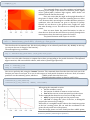
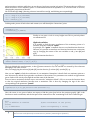
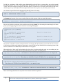
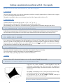
Solving a maximization problem with R - User-guide By Maria Corina Greab, Laura Montenovo, and Maria Pugliesi 1. Introduction The aim of this user-guide is to solve an optimization problem, to display graphically the solutions, and to suggest to users some helpful commands and tricks. The guide is intended for those users having at least a little bit of grasp with the basics of R. 2. Inputing the data Consider a function 𝒇 such that 𝒇(𝒙, 𝒚) = 𝟐 ⋅ 𝒙 ⋅ 𝒚𝟐 + 𝟐 ⋅ 𝒙𝟐 ⋅ 𝒚 + 𝒙 ⋅ 𝒚 We must find the coordinates of the stationary points and then classify them. The first thing to do is to define our 2-variable function, paying attention to brackets and signs, and call it f. > f <- function(x,y) 2*x*(y**2)+2*(x**2)*y+x*y in R performs computations in the following order: powers, multiplications and divisions, sums and subtractions. Now, we want R to assign values to 𝒙 and 𝒚 (we assign 𝒚 values only in the two variable case), through “seq”: > x<- seq(-0.5,0.5, len=200) > y<- seq(-0.5,0.5, len=200) 𝒙 is a sequence of 200 components (len=200) going from -0.5 up to 0.5. Such high choice of sequence length will allow us to produce a sufficiently precise and detailed graph. The same procedure is applied to define the variable𝒚. Since we have a two variables function, we need to define the variable z= 𝒇(𝒙, 𝒚) which corresponds to the values of the function for each pair of 𝒙 and 𝒚 that satisfies 𝒇(𝒙, 𝒚). > z <- outer(x,y,f) The outer command computes a matrix with all the values of 𝒇 for all pairs of 𝒙 and𝒚. To see the proper structure of the matrix, we can use “str(z)” (structure of z) We are now ready to plot the graph of this 3-dimensional function. 3. Graphs To take a look at the 3-dimensional image, we can use the command “persp” (perspective). > persp(x,y,z, theta=-30,phi=15,ticktype="detailed") 𝒙, 𝒚, 𝒛 are our three variables, theta=-30,phi=15 are the coordinates of the angles from which we look at the graph, and ticktype="detailed" displays the numerical values of the variables on the 3 axes. The “persp” command gives us an accurate overview of the shape of our function but this is not enough to find optimizers. For this purpose, we can use the “image” command, with 𝒙, 𝒚, 𝒛 being the three variables of the function𝒇. 1 CompTools a.a. 2011.2012 Maria Corina Greab (832579) Laura Montenovo (832617) Maria Pugliesi (835310) > image(x,y,z) This command allows us to detect minima and maxima by showing us the height of the function at different points: lighter colors (yellow/white) indicate high regions, while darker red indicates that the function decreases. Here, we notice that the angle at the upright boundary of the picture is almost “white”, while the remaining three are more “red”. However, this is not enough to conclude that these points are optimizers, since the function can grow or decrease to infinity. Instead, we can observe on the picture some “bright red” parts that meet forming a cross. This allows us to identify three saddle points. Now we must obtain the partial derivatives in order to draw the zero level sets that will show us precisely, through their intersections, where the stationary points are located. The partial derivative with respect to 𝒙 in R is: >fx <- function(x,y,h=0.001) (f(x+h,y)-f(x,y))/h This describes the incremental ratio. We shock 𝒙 by adding to it an arbitrarily small value, 𝒉(= 𝟎. 𝟎𝟎𝟏). In this way, we compute the rate of change (of the function). The same applies to 𝒚, as follows: >fy <- function(x,y,h=0.001) (f(x,y+h)-f(x,y))/h We now re-use the other function to compute the 𝒛 values corresponding to the partial derivatives. Thus 𝒛𝒇𝒙 and 𝒛𝒇𝒚 are matrices, 400 rows and 400 columns, with values of 𝒇𝒙 and 𝒇𝒚 respectively. >zfx <- outer(x,y,fx) >zfy <- outer(x,y,fy) Now we are perfectly able, using the “contour” function. This command draws lines that show the level sets of the function you insert as an input. If we use it with respect to both partial derivatives at the zero level, it becomes possible to see the stationary points, which are: * Saddle points where the lines cross; *Maxima and minima where we observe small circles. >contour(x,y,zfx,level=0) >contour(x,y,zfy,level=0, add=T, col=”red”) When giving the command we write: the two variables, 𝒙 and 𝒚; the function for which we want to see the level sets. level =0 because we are not interested just in the others. To the command that draws the zero level sets of zfy, we add: add=T to impose this graph over the previous one; col=”red” to change the colors of the line, to distinguish properly the contours for 𝒇𝒙 and 𝒇𝒚. Afterwards, it is straightforward to observe the 4 stationary points at the four crossing points. We can read the coordinates of the points directly on the axis of the pictures. From the image picture we have found just three saddle points, 2 CompTools a.a. 2011.2012 Maria Corina Greab (832579) Laura Montenovo (832617) Maria Pugliesi (835310) and no maxima or minima, while here we see the zero level sets crossing in 4 points. This means that we still do not know the nature of one stationary point. To understand what kind of optimizer it is, we must zoom on its area, changing the proportions of the axis. We do this through “seq” (choosing a shorter interval for x and y), and defining 𝒛 correspondingly. >x <- seq(-0.2,0,len=400) >y <- seq(-0.2,0,len=400) >z<- outer(x,y,f) Looking at the picture of both colors and contours, we will identify the “misterious” point. >image(x,y,z) >contour(x,y,z,add=T) Finally, we can spot a circle in a very bright area. This is precisely where our maximum lies. Algebraic solution: It is possible to find the exact coordinates of the stationary points of a function, using the command “optim”. In principle, the “optim” command does not read multivariate functions. However, it is possible to transform our bivariate function into a univariate one, by changing the names of the two variables x and y, into 𝒙[𝟏] and 𝒙[𝟐]. The new function therefore is: >fbb<-function(x) f(x[1],x[2]) The logic behind this transformation, is that [ ] means extraction. So, 𝒙[𝟏] and 𝒙[𝟐] are viewed by R as elements belonging to the same vector 𝒙. Here, we simply plug the values 𝒙[𝟏] and 𝒙[𝟐] into the function 𝒇, so that 𝒙[𝟏]= 𝒙, and 𝒙[𝟐] = 𝒚. Next, we use “optim” to find the coordinates of our maximizer. Remember is that R finds one stationary point at a time. Moreover, by default R just givesthe coordinates of the minima. Two parameters are needed: an approximate guess of where the critical point might be and the name of the function. Since we have a maximizer, the best way to overcome the “minimizer-default” of R is to reverse the function down, so that the original minimizer becomes now a maximizer. This is done by changing the sign of the value corresponding to the parameter “fnscale”. >optim(c(0.5,0.5),gb,control=list(fnscale=-1)) Here, the vector is our guess of where we expect to find the point (just look at the previous graph). “𝒈𝒃” is the function we need to maximize, and the last part of the command is to the “maximizing trick”. Here is what we get: $par [1] -0.1666634 -0.1666765 $value [1] 0.009259259 3 #(the coordinates of the point) #(the corresponding z value) CompTools a.a. 2011.2012 Maria Corina Greab (832579) Laura Montenovo (832617) Maria Pugliesi (835310) To find the coordinates of the saddle points algebraically, we should solve a system where we set both partial derivatives equal to zero. This is not possible in R. We minimize the sum of the square partial derivatives with “optim”. This sum is always non-negative. The points where it is equal to zero are exactly where both (second order, considering the very initial objective function) partial derivatives are equal to zero, then the system is solved. Let's define the partial derivatives plugging 𝒙[𝟏] and 𝒙[𝟐] instead of 𝒙 and 𝒚. >fxb <- function(x) fx(x[1],x[2]) >fyb <- function(x) fy(x[1],x[2]) Call sumssq the function of the vector 𝒙 made of the sum of the squares of the two partial derivatives. >sumssq <- function(x) fxb(x)**2+fyb(x)**2 Now we can find the coordinates of the saddle points through “optim”. We do exactly the same thing for all three points, just changing the guess of their locations, according to the graphs >optim(c(0.1,0.1),sumssq) $par [1] 1.910525e-06 -1.277307e-05 optim(c(-0.4,0.1),sumssq) $par [1] -5.010126e-01 -4.415738e-06 optim(c(0.1,-0.4),sumssq) $par [1]-4.415738e-06 -5.010126e-01 #(this is almost 0,0) #(this is almost 0.5,0) #(this is almost 0,0.5) Now please recall what is written at about half of the second page. We should make sure that the function increases or decreases to infinity at the angles of the pictures, in ensure that we have found ALL the stationary points of the function, and that none is hidden beyond the boarder of our graphs. We maximize the “white angle” and minimize the other three (to understand what angle we are working on, just have a look at the vector c that indicates approximately where we place our initial guess): >optim(c(-0.4,0.4),fbb) #The values are: 5.457516e+53 and 5.399318e+53 => 𝒙 → +∞ and y-> +∞ >optim(c(0.4,-0.4),fb) #The values are 4.804367e+54 and -4.727385e+54 => x-> +∞ and y-> -∞. >optim(c(0.4,0.4),fb,control=list(fnscale=-1)) # The values are -4.727385e+54 and 4.804367e+54 => x-> -∞ and y-> +∞. >optim(c(-0.4,-0.4),fb)# The values are -1.185271e+54 and -6.367610e+54 =>x-> -∞ and y-> -∞. These results imply that there are no points of our interest outside our pictures. 4 CompTools a.a. 2011.2012 Maria Corina Greab (832579) Laura Montenovo (832617) Maria Pugliesi (835310)