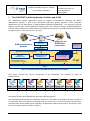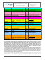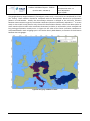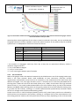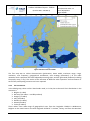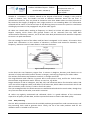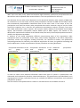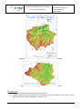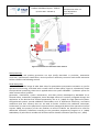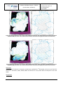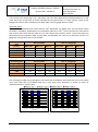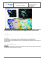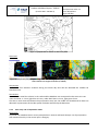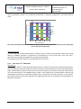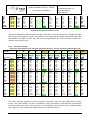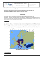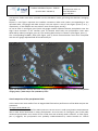
1
Product Validation Report for product H01 – PR-OBS-1 Version 1.1, 30 September 2011 EUMETSAT Satellite Application Facility on Support to Operational Hydrology and Water Management Product Validation Report (PVR-01) for product H01 (PR-OBS-1) Precipitation rate at ground by MW conical scanners Reference Number: Issue/Revision Index: Last Change: About this document SAF/HSAF/PVR-01/1.1 1.1 30 September 2011 This Document has been prepared by the Product Validation Cluster Leader, with the support of the Project Management Team and of the Validation and Development Teams of the Precipitation Cluster Product Validation Report - PVR-01 (Product H01 – PR-OBS-1) Doc.No: SAF/HSAF/PVR-01/1.1 Issue/Revision Index: 1.1 Date: 30/09/2011 Page: 2/183 DOCUMENT CHANGE RECORD Issue / Revision Date Description 1.0 16/05/2011 Baseline version prepared for ORR1 Part 2. Obtained by PVR-01 delivered during the Development Phase. 1.1 30/09/2011 Updates, acknowledging ORR1 Part 2 review board recommendation 1.2 16/01/2012 Minor adjustments: Document reference number as “PVR-01” instead of “PVR” Product Validation Report - PVR-01 (Product H01 – PR-OBS-1) Doc.No: SAF/HSAF/PVR-01/1.1 Issue/Revision Index: 1.1 Date: 30/09/2011 Page: 3/183 Index 1 2 The EUMETSAT Satellite Application Facilities and H-SAF ............................................................... 14 Introduction to product PR-OBS-1 ................................................................................................... 15 2.1 Sensing principle ....................................................................................................................... 15 2.2 Algorithm principle ................................................................................................................... 16 2.3 Main operational characteristics .............................................................................................. 17 3 Validation strategy, methods and tools ........................................................................................... 18 3.1 Validation team and work plan ................................................................................................. 18 3.2 Validation objects and problems .............................................................................................. 20 3.3 Validation methodology............................................................................................................ 20 3.4 Ground data and tools used for validation ............................................................................... 21 3.5 Spatial interpolation for rain gauges ........................................................................................ 24 3.6 Techniques to make observation comparable: up-scaling technique for radar data............... 25 3.7 Temporal comparison of precipitation intensity ...................................................................... 27 3.8 Large statistic: Continuous and multi-categorical .................................................................... 27 3.9 Case study analysis.................................................................................................................... 32 4 Ground data used for validation activities ....................................................................................... 32 4.1 Introduction .............................................................................................................................. 32 4.2 Rain Gauge in PPVG .................................................................................................................. 32 4.2.1 The networks ..................................................................................................................... 32 4.2.2 The instruments ................................................................................................................ 34 4.2.3 Data processing ................................................................................................................. 35 4.2.4 Some conclusions .............................................................................................................. 36 4.3 Radar data in PPVG ................................................................................................................... 37 4.3.1 The networks ..................................................................................................................... 37 4.3.2 The instruments ................................................................................................................ 38 4.3.3 Data processing ................................................................................................................. 39 4.3.4 Some conclusions .............................................................................................................. 40 4.4 Rain gauge and radar data integrated products in PPVG ......................................................... 43 4.4.1 INCA system....................................................................................................................... 43 4.4.2 RADOLAN system .............................................................................................................. 44 4.4.3 Some conclusions .............................................................................................................. 47 4.5 Ground data in Belgium (IRM) .................................................................................................. 48 4.5.1 Radar data ......................................................................................................................... 48 4.6 Ground data in Bulgaria (NIMH) ............................................................................................... 49 4.6.1 Rain gauge ......................................................................................................................... 49 4.7 Ground data in Germany (BfG) ................................................................................................. 51 4.7.1 Rain gauge ......................................................................................................................... 51 4.7.2 Radar data ......................................................................................................................... 52 4.8 Ground data in Hungary (OMSZ)............................................................................................... 54 4.8.1 Radar data ......................................................................................................................... 54 4.9 Ground data in Italy (DPC, Uni Fe) ............................................................................................ 57 4.9.1 Rain gauge ......................................................................................................................... 57 4.9.2 Radar data ......................................................................................................................... 59 Product Validation Report - PVR-01 (Product H01 – PR-OBS-1) Doc.No: SAF/HSAF/PVR-01/1.1 Issue/Revision Index: 1.1 Date: 30/09/2011 Page: 4/183 4.10 Ground data in Poland (IMWM) ............................................................................................... 67 4.10.1 Rain gauge ......................................................................................................................... 67 4.11 Ground data in Slovakia (SHMU) .............................................................................................. 69 4.11.1 Rain gauge ......................................................................................................................... 69 4.11.2 Radar data ......................................................................................................................... 70 4.12 Ground data in Turkey .............................................................................................................. 73 4.12.1 Rain gauge ......................................................................................................................... 73 4.13 Conclusions ............................................................................................................................... 77 5 Validation results: case study analysis ............................................................................................. 78 5.1 Introduction .............................................................................................................................. 78 5.2 Case study analysis in Belgium (IRM) ........................................................................................ 79 5.2.1 Case study: 14th -17th of August 2010 ............................................................................... 79 5.2.2 Case study: 22nd -24th of August 2010 .............................................................................. 82 5.2.3 Case study: 12nd - 15th of November 2010 (h01) ............................................................... 85 5.3 Case study analysis in Germany (BfG) ....................................................................................... 89 5.3.1 Case study: 7th of August 2010 (River Neiße, Oder, Spree and Elbe catchments) ............ 89 5.3.2 Case study: 3rd of June 2010 (River Danube catchment) .................................................. 94 5.3.3 Case study: 5th - 6th of December 2010 (River Rhine catchment) ..................................... 97 5.4 Case study analysis in Hungary (OMSZ) .................................................................................. 102 5.4.1 Case study: 5th of May 2010 ............................................................................................ 102 5.4.2 Case study: 18th of July 2010 ........................................................................................... 103 5.4.3 Case study: 10th of September 2010 .............................................................................. 104 5.5 Case study analysis in Italy (Uni Fe) ........................................................................................ 106 5.5.1 Case study: 6th of July 2010 ............................................................................................. 106 5.6 Case study analysis in Poland (IMWM) ................................................................................... 109 5.6.1 Case study: 15th of August 2010 ...................................................................................... 109 5.6.2 Case study: 17th of May 2010 .......................................................................................... 112 5.7 Case study analysis in Slovakia................................................................................................ 116 5.7.1 Case study: 15th of August 2010 ...................................................................................... 116 5.8 Case study analysis in Turkey (ITU) ......................................................................................... 120 5.8.1 Case study: 20th of October 2010 .................................................................................... 120 5.9 Conclusions ............................................................................................................................. 123 6 Validation results: long statistic analysis........................................................................................ 124 6.1 Introduction ............................................................................................................................ 124 6.2 The continuous statistic .......................................................................................................... 125 6.2.1 The winter period ............................................................................................................ 125 6.2.2 The spring period............................................................................................................. 126 6.2.3 The summer period ......................................................................................................... 127 6.2.4 The autumn period .......................................................................................................... 128 6.2.5 The annual average ......................................................................................................... 129 6.3 The multi-categorical statistic ................................................................................................. 130 6.3.1 Radar validation............................................................................................................... 130 6.3.2 Rain gauge validation ...................................................................................................... 131 6.4 User requirement compliance ................................................................................................ 131 7 Conclusions..................................................................................................................................... 132 7.1 Summary conclusions on the status of product validation .................................................... 132 7.2 Next steps ............................................................................................................................... 133 Product Validation Report - PVR-01 (Product H01 – PR-OBS-1) Doc.No: SAF/HSAF/PVR-01/1.1 Issue/Revision Index: 1.1 Date: 30/09/2011 Page: 5/183 8 Annex 1: Status of working group .................................................................................................. 135 9 Annex 2: Working Group 1 “Rain gauge data” ............................................................................... 135 10 Annex 3: Working Group 2 “Radar data” ....................................................................................... 142 11 Annex 4: Study on evaluation of radar measurements quality indicator with regards to terrain visibility ................................................................................................................................................... 150 12 Annex 5: Working Group 3 “INCA Precipitation for PPV” .............................................................. 156 13 Annex 6: Working Group 4: “PR-ASS-1 (COSMO grid) validation” ................................................. 170 14 Annex 7: Working Group 5: “Geographical maps – distribution of error” .................................... 173 15 Annex 8: Comments on the Validation Results for Products PR-OBS-1, PR-OBS-2 And PR-OBS-3 178 Product Validation Report - PVR-01 (Product H01 – PR-OBS-1) Doc.No: SAF/HSAF/PVR-01/1.1 Issue/Revision Index: 1.1 Date: 30/09/2011 Page: 6/183 List of tables Table 1 H-SAF Products List ...................................................................................................................... 15 Table 2 List of the people involved in the validation of H-SAF precipitation products ........................... 19 Table 3 Number and density of raingauges within H-SAF validation Group............................................ 22 Table 4 Summary of the raingauge characteristics .................................................................................. 23 Table 5 Data pre-processing strategies .................................................................................................... 25 Table 6 Classes for evaluating Precipitation Rate products ..................................................................... 28 Table 7 Number and density of raingauges within H-SAF validation Group............................................ 34 Table 8 Summary of the raingauge characteristics .................................................................................. 35 Table 9 Data pre-processing strategies .................................................................................................... 36 Table 10 Matching strategies for comparison with H01 and H02 ........................................................... 36 Table 11 Inventory of the main radar data and products characteristics in Belgium, Italy and Hungary 42 Table 12 Inventory of the main radar data and products characteristics in Poland, Slovakia and Turkey .................................................................................................................................................................. 42 Table 13 INCA Questionnaire ................................................................................................................... 46 Table 14 Precipitation data used at BfG for validation of H-SAF products .............................................. 51 Table 15 Location of the 16 meteorological radar sites of the DWD ....................................................... 53 Table 16 Main characteristics of the Hungarian radar network .............................................................. 55 Table 17 Characteristics of the three radar instruments in Hungary ...................................................... 55 Table 18 Characteristics of the SHMÚ radars .......................................................................................... 71 Table 19 QA flags descriptions (modified from Shafer et al., 1999) ........................................................ 74 Table 20 Scores obtained with the comparison with radar data (* in mm h-1) ...................................... 81 Table 21 Scores obtained with the comparison with radar data (* in mm h-1) ...................................... 84 Table 22 Scores obtained with the comparison with radar data (* in mm h-1) ...................................... 88 Table 23 Hourly precipitation sum [mm] for H01 satellite data (crosses, time stamp 2010-08-07 05:43 UTC) and for RADOLAN-RW (left, filled raster, 2010-08-07 05:50 UTC) and station data (right, dots, 2010-08-07 06:00 UTC) ............................................................................................................................ 91 Table 24 Results of the categorical statistic of the validation for whole month August 2010 ................ 92 Table 25 Continuous statistic ................................................................................................................... 93 Table 26 Results of the categorical validation statistic of case study 3rd June 2010 .............................. 95 Table 27 Results of the categorical statistic of the validation for whole month June 2010 .................... 96 Table 28 Continuous statistic ................................................................................................................... 97 Table 29 Results of the categorical validation statistic of case study5/6th December 2010 ................ 100 Table 30 Results of the categorical statistic of the validation for whole month December 2010 ........ 100 Table 31 Continuous statistic ................................................................................................................. 101 Table 32 Results of the categorical statistics obtained for PR-OBS-1 .................................................... 111 Table 33 Results of the categorical statistics obtained for PR-OBS-1 .................................................... 115 Table 34 Scores for continuous statistics ............................................................................................... 119 Table 35 Scores for dichotomous statistics ............................................................................................ 119 Table 36 Statistic scores for H01 ............................................................................................................ 123 Table 37 split in four sections, one for each season, reports the Country/Team results side to side. . 125 Table 38 The main statistical scores evaluated by PPVG for H01 during the winter period. Rain rates lower than 0.25 mm/h have been considered no rain .......................................................................... 126 Table 39 The main statistical scores evaluated by PPVG for H01 during the spring period. Rain rates lower than 0.25 mm/h have been considered as no rain ...................................................................... 127 Product Validation Report - PVR-01 (Product H01 – PR-OBS-1) Doc.No: SAF/HSAF/PVR-01/1.1 Issue/Revision Index: 1.1 Date: 30/09/2011 Page: 7/183 Table 40 The main statistical scores evaluated by PPVG for H01 during the summer period. Rain rates lower than 0.25 mm/h have been considered as no rain ...................................................................... 128 Table 41 The main statistical scores evaluated by PPVG for H01 during the autumn period. Rain rates lower than 0.25 mm/h have been considered as no rain ...................................................................... 129 Table 42 The main statistical scores evaluated by PPVG for H01 during one year of data 1st December 2009- 30th November 2010 . Rain rates lower than 0.25 mm/h have been considered as no rain ..... 129 Table 43 The averages POD, FAR and CSI deduced comparing H01 with radar data ............................ 130 Table 44 The contingency table for the three precipitation classes defined in fig. 11 of Chapter 3 evaluated by comparing H01 with radar data........................................................................................ 130 Table 45 The averages POD, FAR and CSI deduced comparing H01 with rain gauge data .................... 131 Table 46 The contingency table for the three precipitation classes defined in Section 3 evaluated by comparing H01 with rain gauge data ..................................................................................................... 131 Table 47 User requirement and compliance analysis for product H01 ................................................. 132 Table 48 Summary of the raingauge characteristics .............................................................................. 138 Table 49 Number and density of raingauges within H-SAF validation Group........................................ 139 Table 50 Data pre-processing strategies ................................................................................................ 140 Table 51 Matching strategies for comparison with H01 and H02 ......................................................... 141 Table 52 Matching strategies for comparison with H03 and H05 ......................................................... 141 Table 53 List of contact persons............................................................................................................. 158 Table 54 Questionnaire .......................................................................................................................... 162 Table 55 List of precipitation events selected for statistical analysis .................................................... 166 Table 56 Mean Residual and Mean Absolute Residual values obtained for three algorithms for spatial interpolation using cross-validation approach....................................................................................... 176 Table 57 Simplified compliance analysis for product PR-OBS 1-2-3 ...................................................... 178 Table 58 Errors of the ground reference provided by all validation groups .......................................... 179 Table 59 RMSE% and standard deviation of interpolation algorithms for 3 different regular grids ..... 182 List of figures Figure 1 Conceptual scheme of the EUMETSAT application ground segment ........................................ 14 Figure 2 Current composition of the EUMETSAT SAF network (in order of establishment) ................... 14 Figure 3 Geometry of conical scanning for SSMIS.................................................................................... 16 Figure 4 Flow chart of the precipitation rate processing chain from SSM/I and SSMIS .......................... 17 Figure 5 Structure of the Precipitation products validation team ........................................................... 18 Figure 6 The network of 3500 rain gauges used for H-SAF precipitation products validation ................ 21 Figure 7 The networks of 54 C-band radars available in ther H-SAF PPVG .............................................. 24 Figure 8 Geometry of conical scanning (left) and IFOV (right) of SSMI .................................................. 25 Figure 9 Left) Gaussian filter – Right) section of gaussian filter .............................................................. 26 Figure 10 Left) Original Gaussian matrix – Right)Reduced matrix to dimensions M xK .......................... 26 Figure 11 Main steps of the validation procedure in the PPVG ............................................................... 29 Figure 12 Rain gauge networks in PPVG .................................................................................................. 33 Figure 13 Correlation coefficient between raingauge pairs as function of the distances between the gauges. Colours refer to the months of the year 2009 ............................................................................ 34 Figure 14 Radar networks in PPVG........................................................................................................... 38 Figure 15 Radar scan procedure............................................................................................................... 39 Product Validation Report - PVR-01 (Product H01 – PR-OBS-1) Doc.No: SAF/HSAF/PVR-01/1.1 Issue/Revision Index: 1.1 Date: 30/09/2011 Page: 8/183 Figure 16 Coverage of Europe by the INCA and RADOLAN systems ........................................................ 43 Figure 17 Procedure of the RADOLAN online adjustment (hourly precipitation amount on 7 August 2004 13:50 UTC) ....................................................................................................................................... 45 Figure 18 Precipitation intensity field from 15 August 2010 15:00 UTC obtained by a) radars, b) interpolated raingauge data, c) INCA analysis and d) PR-OBS-1 product ................................................ 47 Figure 19 Meteorological radar in Belgium .............................................................................................. 48 Figure 20 Distribution of the raingauge stations of Iskar River Basin ...................................................... 49 Figure 21 Distribution of the raingauge stations of Chepelarska River Basin .......................................... 50 Figure 22 Distribution of the raingauge stations of Varbica River Basin ................................................. 50 Figure 23 Network of rain gauges in Germany ........................................................................................ 52 Figure 24 Pluvio with Remote Monitoring Module.................................................................................. 52 Figure 25 Left: radar compound in Germany (March 2011) ; Right: location of ombrometers for online calibration in RADOLAN; squares: hourly data provision (about 500), circles: event-based hourly data provision (about 800 stations .................................................................................................................. 53 Figure 26 Flowchart of online calibration RADOLAN (DWD, 2004) ......................................................... 54 Figure 27 location and coverage of the three Hungarian radars ............................................................. 54 Figure 28 Correlation between rainrates detected by two close by stations as function of the distance between the two stations. Colors refer to the month along 2009 .......................................................... 57 Figure 29 Distribution of the raingauge stations of the Italian network collected by DPC ..................... 58 Figure 30 Italian radar network coverage ................................................................................................ 59 Figure 31 Graphical mosaic of reflectivity (CAPPI at 2000 m) for the event of 04/18/08 at 0015 U.T.C 60 Figure 32 Architecture of the Italian radar network ................................................................................ 61 Figure 33 Schematic representation of radar data processing chain ...................................................... 62 Figure 34 Measured (upper panel) and attenuation corrected (lower panel) PPI (1.0 deg) of reflectivity observed on 09/14/08 at 0500 U.T.C. by the polarimetric radar operated by Piemonte and Liguria regions ...................................................................................................................................................... 63 Figure 35 Hydrometeor classes as detected by the classification algorithm starting from the radar variables observed on 09/14/08 at 0500 U.T.C. by the polarimetric radar operated by Piemonte and Liguria regions .......................................................................................................................................... 64 Figure 36 Measured (upper panel) and VPR corrected (lower panel) PPI of reflectivity observed on 03/25/07 at 0930 U.T.C. by the polarimetric radar located in Gattatico (Emilia Romagna, Italy). ......... 66 Figure 37 Cumulated radar rainfall estimates versus gage measurements for the event observed on 06/01/2006 by the dualpolarized radar located in Settepani (Liguria, Italy). .......................................... 67 Figure 38 ATS national network in Poland ............................................................................................... 68 Figure 39 Map of SHMÚ rain gauge stations: green – automatic (98), blue – climatological (586), red hydrological stations in H-SAF selected test basins (37) .......................................................................... 69 Figure 40 Map of SHMÚ radar network; the rings represent maximum operational range – 240 km for radar at Maly Javornik (left), 200 km for radar at Kojsovska hola (right) ................................................ 70 Figure 41 Map of relative RMSE (left) and Mean Error (right) over the SHMÚ radar composite ........... 72 Figure 42 Automated Weather Observation System (AWOS) station distribution in western part of Turkey ....................................................................................................................................................... 73 Figure 43 H01 and H02 products footprint centers with a sample footprint area as well as the Awos ground observation sites .......................................................................................................................... 75 Figure 44 Meshed structure of the sample H01 and H02 products footprint ......................................... 76 Figure 45 Synoptic situation on 15 August 2010 at 6 UTC (zoom in the surface map)............................ 79 Product Validation Report - PVR-01 (Product H01 – PR-OBS-1) Doc.No: SAF/HSAF/PVR-01/1.1 Issue/Revision Index: 1.1 Date: 30/09/2011 Page: 9/183 Figure 46 H01 image of August 15th, 2010 at 16.41 (left) compared with upscaled radar at 16.40 (right). The scale corresponds to thresholds of 0.1, 1., and 10. mm h-1. The product matches the rainfall pattern quite good ....................................................................................................................... 80 Figure 47 H01 image of August 16th, 2010 at 4.56 (left) compared with upscaled radar at 4.55 (right). The scale corresponds to thresholds of 0.1, 1., and 10. mm h-1. Also in this case the matching is quite good .......................................................................................................................................................... 80 Figure 48 H01 image of August 14th, 2010 at 6.06 (left) compared with upscaled radar at 6.05 (right). The scale corresponds to thresholds of 0.1, 1., and 10. mm h-1 ............................................................. 81 Figure 50 Surface map on 22 August 2010 at 06 UTC (MSLP and synoptic observations) ...................... 82 Figure 49 Time evolution of fraction area with rain measured by radar > 0.25 mm/h and Equitable Threat Score (ETS) during the present case study ................................................................................... 82 Figure 51 H01 image of August 23th, 2010 at 16.18 (left) compared with upscaled radar at 16.20 (right). The scale corresponds to thresholds of 0.1, 1., and 10. mm h-1. The product matches the rainfall pattern quite good, but underestimates higher rain amounts.................................................... 83 Figure 52 H01 image of August 23th, 2010 at 5.53 (left) compared with upscaled radar at 5.55 (right). The scale corresponds to thresholds of 0.1, 1., and 10. mm h-1. ............................................................ 84 Figure 53 Time evolution of fraction area with rain measured by radar > 0.25 mm/h and Equitable Threat Score (ETS) during the present case study ................................................................................... 85 Figure 54 Surface map on 13 November 2010 at 06 UTC (MSLP and synoptic observations) ................ 86 Figure 55 H01 image of November 13th, 2010 at 5.28 (left) compared with upscaled radar at 5.30 (right). The scale corresponds to thresholds of 0.1, 1., and 10. mm h-1 ................................................. 87 Figure 56 H01 image of November 13th, 2010 at 15.17 (left) compared with upscaled radar at 15.15 (right). The scale corresponds to thresholds of 0.1, 1., and 10. mm h-1 ................................................. 87 Figure 57 H01 image of November 13th, 2010 at 6.03 (left) compared with upscaled radar at 6.05 (right). ....................................................................................................................................................... 88 Figure 58 Time evolution of fraction area with rain measured by radar > 0.25 mm/h and Equitable Threat Score (ETS) during the present case study ................................................................................... 89 Figure 59 Synopsis for Central Europe for 07th August 2010 (FU - Berlin, http://wkserv.met.fuberlin.de) .................................................................................................................................................. 90 Figure 60 two-day totals (ending at 9th August, 0 UTC) interpolated on a 1°x1° evaluation grid as derived from SYNOP messages (Global Precipitation Climatology Centre, GPCC operated by DWD .... 90 Figure 61 Hourly precipitation sum [mm] for H01 satellite data (crosses, time stamp 2010-08-07 05:43 UTC) and for RADOLAN-RW (left, filled raster, 2010-08-07 05:50 UTC) and station data (right, dots, 2010-08-07 06:00 UTC) ............................................................................................................................ 91 Figure 62 Contingency table statistic of rain rate [mmh-1] for PR-OBS1 vs. radar data Left: for 7th August 2010, Right: for whole August 2010............................................................................................. 92 Figure 63 Contingency table statistic of rain Rate [mmh-1] for PR-OBS1 vs. rain gauge data. Left: for 7th August 2010, Right: for whole August 2010............................................................................................. 93 Figure 64 Synopsis for Central Europe for 03rd June 2010 (FU Berlin, http://wkserv.met.fu-berlin.de)94 Figure 65 12h totals of precipitation(ending at 3rd June 2010, 7 UTC) ................................................... 94 Figure 66 Hourly precipitation sum [mm] for H01 satellite data (crosses, time stamp 2010-06-03 07:17 UTC) and for RADOLAN-RW (left, filled raster, 2010-06-03 07:50 UTC) and station data (right, dots 2010-06-03 08:00 UTC) ............................................................................................................................ 95 Figure 67 Contingency table statistic of Rain Rate [mmh-1] for PR-OBS1 vs. radar data ........................ 96 Figure 68 Contingency table statistic of rain rate [mmh-1] for PR-OBS1 vs. rain gauge data ................. 96 Figure 69 Synopsis for Central Europe for 05th December 2010 (FU Berlin, http://wkserv.met.fuberlin.de) .................................................................................................................................................. 98 Product Validation Report - PVR-01 (Product H01 – PR-OBS-1) Doc.No: SAF/HSAF/PVR-01/1.1 Issue/Revision Index: 1.1 Date: 30/09/2011 Page: 10/183 Figure 70 96h totals of precipitation ........................................................................................................ 98 Figure 71 Hourly precipitation sum [mm] for H01 satellite data (crosses, time stamp 2010-12-05 07:027 UTC) and for RADOLAN-RW (left, filled raster, 2010-12-05 07:50 UTC) and station data (right, dots 2010-12-05 08:00 UTC) ............................................................................................................................ 99 Figure 72 Hourly precipitation sum [mm] for H01 satellite data (crosses, time stamp 2010-12-06 06:49 UTC) and for RADOLAN-RW (left, filled raster, 2010-12-06 06:50 UTC) and station data (right, dots 2010-12-06 07:00 UTC) ............................................................................................................................ 99 Figure 73 Contingency table statistic of Rain Rate [mmh-1] for PR-OBS1 vs. radar data ...................... 100 Figure 74 Contingency table statistic of rain rate [mmh-1] for PR-OBS1 vs. rain gauge data ............... 101 Figure 75 Synoptic chart at 00 UTC on 5 May 2010 ............................................................................... 102 Figure 76 Precipitation rate from the Hungarian radar network at its original resolution (upper right panel), H01 product (upper left panel) , operational png (lower left panel), SAFNWC Cloud Type (CT) product (lower right) .............................................................................................................................. 103 Figure 77 Synoptic chart at 00 UTC on 18th of July 2010 ...................................................................... 104 Figure 78 H01 product (left panel), Cloud type from NWC SAF (right panel). Precipitation rate from the H ungarian radar network at its original resolution (in middle) ............................................................ 104 Figure 79 Synoptic chart at 00 UTC on 10th of September 2010 .......................................................... 105 Figure 80 Precipitation rate from the Hungarian radar network at its original resolution at 6:45 UTC) (right panel), H01 product (left panel) at 6:45 UTC ............................................................................... 105 Figure 81 H01 precipitation map at 15:42 UTC ...................................................................................... 108 Figure 82 Raingauges hourly precipitation cumulated at 16:00 UTC (right) of 06 July 2010. Please note different colour scales ............................................................................................................................ 108 Figure 83 Synoptic chart at 1200 UTC on 15th of August 2010 ............................................................. 109 Figure 84 Total lighting map of Poland showing electrical activity between 1445 and 1515 UTC on 15th of August 2010 ....................................................................................................................................... 110 Figure 85 PR-OBS-1 at 1459 UTC on the 15th of August 2010 (right panel) and 10 minute precipitation interpolated from RG data from 1500 UTC (left panel) ......................................................................... 110 Figure 86 Scatter plot for measured (RG) and satellite derived (H01) rain rate obtained for all H01 data on the 15th of August 2010.................................................................................................................... 111 Figure 87 Percentage distribution of PR-OBS-1 precipitation classes in the rain classes defined using rain gauges (RG) data on the 15th of August 2010 ................................................................................ 112 Figure 88 Synoptic chart at 0000 UTC on 17th of May 2010. Source: IMWM ....................................... 113 Figure 89 PR-OBS-1 at 0453 UTC on the 17th of May 2010 (right panel) and 10 minute precipitation interpolated from RG data from 0500 UTC (left panel) ......................................................................... 114 Figure 90 PR-OBS-1 at 0546 UTC on the 17th of May 2010 (right panel) and 10 minute precipitation interpolated from RG data from 0550 UTC (left panel) ......................................................................... 114 Figure 91 Scatter plot for measured (RG) and satellite derived (H-01) rain rate obtained for all PR-OBS1 data on the 17th of May 2010............................................................................................................. 115 Figure 92 Percentage distribution of PR-OBS-1 precipitation classes in the rain classes defined using rain gauges (RG) data on the 17th of May 2010 .................................................................................... 116 Figure 93 Synoptic situation on 15 August 2010 at 0:00 UTC ................................................................ 116 Figure 94 Instantaneous precipitation field on 15 August 2010 at 07:05 UTC (top row) and 15:00 UTC (second row) derived by SHMU radar network (left column) and H01 product (right column) ........... 118 Figure 95 Comparison of radar precipitation field from 15 August 2010 at 07:05 UTC in original 1 km resolution (left) and upscaled into the satellite grid of the 07:04 UTC passage of DMSP16 ................. 120 Figure 96 Atmospheric condition (20.10.2010; 06:00 GMT).................................................................. 120 Figure 97 Atmospheric condition (20.10.2010; 12:00 GMT).................................................................. 121 Product Validation Report - PVR-01 (Product H01 – PR-OBS-1) Doc.No: SAF/HSAF/PVR-01/1.1 Issue/Revision Index: 1.1 Date: 30/09/2011 Page: 11/183 Figure 98 Comparison of H01 product and rain gauge (RG) .................................................................. 122 Figure 99 Scatter diagram of rain gauge and H01 product (Red line is 45 degree line) ........................ 122 Figure 100 Rain gauge networks in PPVG .............................................................................................. 137 Figure 101 Correlation coefficient between raingauge pairs as function of the distances between the gauges. Colours refer to the months of the year 2009 .......................................................................... 139 Figure 102 Distribution of rain gauges according their altitude above the sea level ............................ 151 Figure 103 Radar horizon model output for Malý Javorník (left) and Kojšovská hoľa (right) radar sites ................................................................................................................................................................ 152 Figure 104 Composite picture of minimum visible height above the surface over the whole radar network. Compositing algorithm selects the minimum value from both radar sites ............................ 152 Figure 105 Distribution of rain gauges according to the minimum visible height of radar beam ......... 153 Figure 106 Scatterplot of log(R/G) versus station altitude shows general underestimation of precipitation by radar ............................................................................................................................. 153 Figure 107 Scatterplot of log(R/G) versus radar beam altitude shows increased underestimation of radar for high and close to zero radar beam elevations ........................................................................ 154 Figure 108 Relative RMSE (left) and Mean Error (right) computed independently for each rain gauge station in radar range and corresponding trend lines extrapolated for beam elevation up to 1500m 155 Figure 109 Final relative root mean square error map of radar measurements with regard to terrain visibility by current radar network of SHMÚ ......................................................................................... 155 Figure 110 Final mean error map of radar measurements with regard to terrain visibility by current radar network of SHMÚ. General underestimation of precipitation by radars is observed ................. 156 Figure 111 Coverage of Europe by the INCA and RADOLAN systems .................................................... 159 Figure 112 Procedure of the RADOLAN online adjustment (hourly precipitation amount on 7 August 2004 13:50 UTC) ..................................................................................................................................... 161 Figure 113 Precipitation intensity field from 15 August 2010 15:00 UTC obtained by a) radars, b) interpolated raingauge data, c) INCA analysis and d) PR-OBS-1 product .............................................. 163 Figure 114 Precipitation intensity field from 15 August 2010 6:00 UTC obtained by a) radars, b) interpolated raingauge data, c) INCA analysis and d) PR-OBS-3 product (5:57 UTC) supplemented with map of minimum visible height above surface level of the SHMU radar network e)............................ 164 Figure 115 As in previous figure except for 8:00 UTC ............................................................................ 165 Figure 116 Comparison of selected statistical scores for the PR-OBS-2 product obtained by different “ground reference” data; valid for event 1 (convective) ....................................................................... 167 Figure 117 As in previous figure except for event 4 (stratiform) ........................................................... 168 Figure 119 The Wideumont radar image of 1/2/2010 (cumulated rainfall in the previous 24 hours, raingauge-adjusted) and upscaled to the COSMO grid.......................................................................... 172 Figure 118 the Wideumont radar image of 1/2/2010 (cumulated rainfall in the previous 24 hours, raingauge-adjusted) ............................................................................................................................... 172 Figure 120 Distribution of the monthly average H-05 3 h cumulated precipitation Mean Error calculated for July 2010 using three methods: a) Ordinary Kriging, b) Natural Neighbour, and c) IDW (2) ................................................................................................................................................................ 175 Figure 121 Cross validation results obtained for three different methods for spatial interpolation .... 176 Figure 122 Example of sampled data for a regular grid. In right on the upper part a detail of field studied, below the original grid of field for step 2 ............................................................................... 181 Figure 123 Randomly distribution of perfect measurement to remap the field on a regular grid ....... 182 Figure 124 STD vs. RMSE% for interpolations by step 2 ........................................................................ 183 Product Validation Report - PVR-01 (Product H01 – PR-OBS-1) Doc.No: SAF/HSAF/PVR-01/1.1 Issue/Revision Index: 1.1 Date: 30/09/2011 Page: 12/183 Acronyms AMSU AMSU-A AMSU-B ATDD AU BfG CAF CDOP CESBIO CM-SAF CNMCA CNR CNRS DMSP DPC EARS ECMWF EDC EUM EUMETCast EUMETSAT FMI FTP GEO GRAS-SAF HDF HRV H-SAF © IDL IFOV IMWM IPF IPWG IR IRM ISAC ITU LATMOS LEO LSA-SAF Météo France METU MHS MSG MVIRI MW NESDIS NMA NOAA NWC-SAF NWP NWP-SAF O3M-SAF OMSZ Advanced Microwave Sounding Unit (on NOAA and MetOp) Advanced Microwave Sounding Unit - A (on NOAA and MetOp) Advanced Microwave Sounding Unit - B (on NOAA up to 17) Algorithms Theoretical Definition Document Anadolu University (in Turkey) Bundesanstalt für Gewässerkunde (in Germany) Central Application Facility (of EUMETSAT) Continuous Development-Operations Phase Centre d'Etudes Spatiales de la BIOsphere (of CNRS, in France) SAF on Climate Monitoring Centro Nazionale di Meteorologia e Climatologia Aeronautica (in Italy) Consiglio Nazionale delle Ricerche (of Italy) Centre Nationale de la Recherche Scientifique (of France) Defense Meteorological Satellite Program Dipartimento Protezione Civile (of Italy) EUMETSAT Advanced Retransmission Service European Centre for Medium-range Weather Forecasts EUMETSAT Data Centre, previously known as U-MARF Short for EUMETSAT EUMETSAT’s Broadcast System for Environmental Data European Organisation for the Exploitation of Meteorological Satellites Finnish Meteorological Institute File Transfer Protocol Geostationary Earth Orbit SAF on GRAS Meteorology Hierarchical Data Format High Resolution Visible (one SEVIRI channel) SAF on Support to Operational Hydrology and Water Management Interactive Data Language Instantaneous Field Of View Institute of Meteorology and Water Management (in Poland) Institut für Photogrammetrie und Fernerkundung (of TU-Wien, in Austria) International Precipitation Working Group Infra Red Institut Royal Météorologique (of Belgium) (alternative of RMI) Istituto di Scienze dell’Atmosfera e del Clima (of CNR, Italy) İstanbul Technical University (in Turkey) Laboratoire Atmosphères, Milieux, Observations Spatiales (of CNRS, in France) Low Earth Orbit SAF on Land Surface Analysis National Meteorological Service of France Middle East Technical University (in Turkey) Microwave Humidity Sounder (on NOAA 18 and 19, and on MetOp) Meteosat Second Generation (Meteosat 8, 9, 10, 11) Meteosat Visible and Infra Red Imager (on Meteosat up to 7) Micro Wave National Environmental Satellite, Data and Information Services National Meteorological Administration (of Romania) National Oceanic and Atmospheric Administration (Agency and satellite) SAF in support to Nowcasting & Very Short Range Forecasting Numerical Weather Prediction SAF on Numerical Weather Prediction SAF on Ozone and Atmospheric Chemistry Monitoring Hungarian Meteorological Service Product Validation Report - PVR-01 (Product H01 – PR-OBS-1) ORR OSI-SAF PDF PEHRPP Pixel PMW PP PR PUM PVR RMI RR RU SAF SEVIRI SHMÚ SSM/I SSMIS SYKE TBB TKK TMI TRMM TSMS TU-Wien U-MARF UniFe URD UTC VIS ZAMG Doc.No: SAF/HSAF/PVR-01/1.1 Issue/Revision Index: 1.1 Date: 30/09/2011 Page: 13/183 Operations Readiness Review SAF on Ocean and Sea Ice Probability Density Function Pilot Evaluation of High Resolution Precipitation Products Picture element Passive Micro-Wave Project Plan Precipitation Radar (on TRMM) Product User Manual Product Validation Report Royal Meteorological Institute (of Belgium) (alternative of IRM) Rain Rate Rapid Update Satellite Application Facility Spinning Enhanced Visible and Infra-Red Imager (on Meteosat from 8 onwards) Slovak Hydro-Meteorological Institute Special Sensor Microwave / Imager (on DMSP up to F-15) Special Sensor Microwave Imager/Sounder (on DMSP starting with S-16) Suomen ympäristökeskus (Finnish Environment Institute) Equivalent Blackbody Temperature (used for IR) Teknillinen korkeakoulu (Helsinki University of Technology) TRMM Microwave Imager (on TRMM) Tropical Rainfall Measuring Mission UKMO Turkish State Meteorological Service Technische Universität Wien (in Austria) Unified Meteorological Archive and Retrieval Facility University of Ferrara (in Italy) User Requirements Document Universal Coordinated Time Visible Zentralanstalt für Meteorologie und Geodynamik (of Austria) Product Validation Report - PVR-01 (Product H01 – PR-OBS-1) 1 Doc.No: SAF/HSAF/PVR-01/1.1 Issue/Revision Index: 1.1 Date: 30/09/2011 Page: 14/183 The EUMETSAT Satellite Application Facilities and H-SAF The “EUMETSAT Satellite Application Facility on Support to Operational Hydrology and Water Management (H-SAF)” is part of the distributed application ground segment of the “European Organisation for the Exploitation of Meteorological Satellites (EUMETSAT)”. The application ground segment consists of a “Central Application Facility (CAF)” and a network of eight “Satellite Application Facilities (SAFs)” dedicated to development and operational activities to provide satellite-derived data to support specific user communities. See fig. 1. EUM Geostationary Systems Systems of the EUM/NOAA Cooperation Data Acquisition and Control other data sources Data Processing EUMETSAT HQ Application Ground Segment Meteorological Products Extraction EUMETSAT HQ Archive & Retrieval Facility (Data Centre) EUMETSAT HQ Centralised processing and generation of products Satellite Application Facilities (SAFs) Decentralised processing and generation of products USERS Figure 1 Conceptual scheme of the EUMETSAT application ground segment Next figure reminds the current composition of the EUMETSAT SAF network (in order of establishment). Nowcasting & Very Short Range Forecasting Ocean and Sea Ice Ozone & Atmospheric Chemistry Monitoring Climate Monitoring Numerical Weather Prediction GRAS Meteorology Land Surface Analysis Operational Hydrology & Water Management Figure 2 Current composition of the EUMETSAT SAF network (in order of establishment) Conceptual scheme of the EUMETSAT application ground segment The H-SAF was established by the EUMETSAT Council on 3 July 2005; its Development Phase started on 1st September 2005 and ended on 31 August 2010. The SAF is now in its first Continuous Development and Operations Phase (CDOP) which started on 28 September 2010 and will end on 28 February 2012 The list of H-SAF products is shown in Table 1: Product Validation Report - PVR-01 (Product H01 – PR-OBS-1) Acronym Doc.No: SAF/HSAF/PVR-01/1.1 Issue/Revision Index: 1.1 Date: 30/09/2011 Page: 15/183 Identifier Name PR-OBS-1 H-01 Precipitation rate at ground by MW conical scanners (with indication of phase) PR-OBS-2 H-02 Precipitation rate at ground by MW cross-track scanners (with indication of phase) PR-OBS-3 H-03 Precipitation rate at ground by GEO/IR supported by LEO/MW PR-OBS-4 H-04 Precipitation rate at ground by LEO/MW supported by GEO/IR (with flag for phase) PR-OBS-5 H-05 Accumulated precipitation at ground by blended MW and IR PR-OBS-6 H-15 Blended SEVIRI Convection area/ LEO MW Convective Precipitation PR-ASS-1 H-06 Instantaneous and accumulated precipitation at ground computed by a NWP model SM-OBS-2 H-08 Small-scale surface soil moisture by radar scatterometer SM-OBS-3 H-16 Large-scale surface soil moisture by radar scatterometer SM-DAS-2 H-14 Liquid root zone soil water index by scatterometer assimilation in NWP model SN-OBS-1 H-10 Snow detection (snow mask) by VIS/IR radiometry SN-OBS-2 H-11 Snow status (dry/wet) by MW radiometry SN-OBS-3 H-12 Effective snow cover by VIS/IR radiometry SN-OBS-4 H-13 Snow water equivalent by MW radiometry Table 1 H-SAF Products List 2 2.1 Introduction to product PR-OBS-1 Sensing principle Product PR-OBS-1 is fundamentally based on the instruments SSM/I and SSMIS flown on the DMSP satellites. These conical scanners provide images with constant zenith angle, that implies constant optical path in the atmosphere and homogeneous impact of the polarisation effects (see Figure 3). Product Validation Report - PVR-01 (Product H01 – PR-OBS-1) Doc.No: SAF/HSAF/PVR-01/1.1 Issue/Revision Index: 1.1 Date: 30/09/2011 Page: 16/183 Figure 3 Geometry of conical scanning for SSMIS Also, conical scanning provides constant resolution across the image, though changing with frequency. It is noted that the IFOV is elliptical, with major axis elongated along the viewing direction and the minor axis along-scan, approximately 3:5 of the major. Its size is dictated by the antenna diameter (actually, the antenna is slightly elliptical, to partially compensate for the panoramic distortion), but also by the portion of antenna effectively illuminated (this enables to obtain the same IFOV for a group of different frequencies, if co-registration is a strong requirement). As for the ‘pixel’, i.e. the area subtended as a consequence of the bi-dimensional sampling rate, the sampling distance along the satellite motion, i.e. from scan line to scan line, is invariably 12.5 km, dictated by the satellite velocity on the ground and the scan rate. Along scan, the sampling rate is selected differently for different frequencies or set of frequencies, as necessary to fulfil the radiometric accuracy requirement and to . minimise aliasing. For more information, please refer to the Products User Manual (specifically, volume PUM-01). 2.2 Algorithm principle The baseline algorithm for PR-OBS-1 processing is described in ATDD-01. Only essential elements are highlighted here. Fig. 04 illustrates the flow chart of the SSM/I-SSMIS processing chain. There is an off-line activity to prepare the Cloud-Radiation Database (CRD) and a real-time activity to exploit the satellite data for the product retrieval. The off-line activities consist of: collecting well-documented meteorological events (analysis or re-analysis); applying a Cloud Resolving Model (CRM) to simulate the cloud microphysics missing in the analysis; applying a Radiative Transfer Model (RTM) to convert the cloud pattern in a pattern of (monochromatic) radiances at all frequencies and polarisations of the SSM/I-SSMIS channels; convoluting the monochromatic radiances with the instrument model so to simulate brightness temperatures comparable with those that would be measured from the satellite; finally collect the simulated TB’s in the Cloud-Radiation Database. Product Validation Report - PVR-01 (Product H01 – PR-OBS-1) Doc.No: SAF/HSAF/PVR-01/1.1 Issue/Revision Index: 1.1 Date: 30/09/2011 Page: 17/183 When the satellite passes, the acquired data are pre-processed by the instrument processor and made available for the precipitation generation chain, that includes: an initial preparation of the dataset to be processed (sea-land mask, emissivity, preventive classification of cloud nature, …); the retrieval algorithm that searches for the maximum-likelihood solution in the hydrometeor profiles available in the CRD, also using the error structure available in a database; the uncertainty estimator, that appends the retrieved precipitation rate with information on likely error; this information is also used for updating the error structure database. OFF-LINE ACTIVITY REAL-TIME ACTIVITY Meteorological events Cloud Resolving Model Actual SSM/I - SSMIS data (pre-processed) Simulated cloud microphysics Radiative Transfer Model Precipitation retrieval model Simulated MW radiances Instrument model Uncertainty estimator model PRECIPITATION RATE Cloud-Radiation Database Error structure database ERROR ESTIMATE Figure 4 Flow chart of the precipitation rate processing chain from SSM/I and SSMIS 2.3 Main operational characteristics The operational characteristics of PR-OBS-1 are discussed in PUM-01. Here are the main highlights. The horizontal resolution ( x) descends from the instrument Instantaneous Field of View (IFOV), the sampling distance (pixel), the Modulation Transfer Function (MTF) and number of pixels to co-process for filtering out disturbing factors (e.g. clouds) or improving accuracy. Conclusion for PR-OBS-1: resolution x ~ 30 km - sampling distance: 16 km. The observing cycle ( t) depends on the instrument swath and the number of satellites carrying the addressed instrument. For PR-OBS-1 there are 4 DMSP satellites but, because of the limited instrument swath, they provide a total service equivalent to that one of two satellites, around 7:00 and 18:00 LST. In average the observing cycle over Europe is t ~ 6 h, with actual interval ranging from 2 to Product Validation Report - PVR-01 (Product H01 – PR-OBS-1) Doc.No: SAF/HSAF/PVR-01/1.1 Issue/Revision Index: 1.1 Date: 30/09/2011 Page: 18/183 10 hours. Gaps are filled by product PR-OBS-2, that also has observing cycle t ~ 6 h, but LST around 9:30 and 14:00, with actual intervals ranging from 4.5 to 7.5 hours. Conclusion: for PR-OBS-1 as stand alone (i.e. from DMSP satellites): cycle t = 6 h, sampling 2 10 h; for the composite PR-OBS-1 + PR-OBS-2 system: cycle t = 3 h, sampling 2 4.5 h. The timeliness ( ) is defined as the time between observation taking and product available at the user site assuming a defined dissemination mean. The timeliness depends on the satellite transmission facilities, the availability of acquisition stations, the processing time required to generate the product and the reference dissemination means. In the case of PR-OBS-1 it is strongly conditioned by the availability of DMSP data at CNMCA, through NOAA and UKMO. The outcome is timeliness ~ 2.5 h. The accuracy (RMS) is the convolution of several measurement features (random error, bias, sensitivity, precision, …). To simplify matters, it is generally agreed to quote the root-mean-square difference [observed - reference values]. The accuracy of a satellite-derived product descends from the strength of the physical principle linking the satellite observation to the natural process determining the parameter. It is difficult to be estimated a-priori: it is generally evaluated a-posteriori by means of the validation activity. 3 3.1 Validation strategy, methods and tools Validation team and work plan To evaluate the satellite precipitation product accuracy a Validation Group has been established by the beginning of the Validation Phase in the H-SAF project. The Precipitation Product Validation team is composed of experts from the National Meteorological and Hydrological Institutes of Belgium, Bulgaria, Germany, Hungary, Italy, Poland, Slovakia, and Turkey (Figure 5). Hydrologists, meteorologists, and precipitation ground data experts, coming from these countries are involved in the product validation activities (Table 2). H01 has been submitted to validation in all these countries except Bulgaria. Until now the Bulgarian data are used only for H05 validation activity according to the Project Plan. Their use in the next months is under consideration. Precipitation Products Validation Group: Italy (DPC) Belgium IRM Bulgaria NIMH-BAS Germany BfG Hungary OMSZ Italy Uni Fe Poland IMWM Slovakia SHMU Turkey ITU TSMS Figure 5 Structure of the Precipitation products validation team Validation team for precipitation products Silvia Puca (Leader) Dipartimento Protezione Civile (DPC) Italy Emanuela Campione Dipartimento Protezione Civile (DPC) Italy [email protected] [email protected] t Gianfranco Vulpiani Dipartimento Protezione Civile (DPC) Italy [email protected] Product Validation Report - PVR-01 (Product H01 – PR-OBS-1) Doc.No: SAF/HSAF/PVR-01/1.1 Issue/Revision Index: 1.1 Date: 30/09/2011 Page: 19/183 Alexander Toniazzo Dipartimento Protezione Civile (DPC) Italy [email protected] Emmanuel Roulin Institut Royal Météorologique (IRM) Belgium [email protected] Angelo Rinollo Institut Royal Météorologique (IRM) Belgium National Institute of Meteorology and Hydrology Bulgarian Academy of Sciences (NIMH-BAS) Bulgaria National Institute of Meteorology and Hydrology Bulgarian Academy of Sciences (NIMH-BAS) Bulgaria Gergana Kozinarova Georgy Koshinchanov [email protected] [email protected] [email protected] Claudia Rachimow Peter Krahe Bundesanstalt für Gewässerkunde (BfG) Germany [email protected] Bundesanstalt für Gewässerkunde (BfG) Germany [email protected] Hungarian Meteorological Service Eszter Lábó (OMSZ) Hungary [email protected] Hungarian Meteorological Service Judit Kerenyi (OMSZ) Hungary [email protected] Ferrara University, Department of Federico Porcu' Physics (UniFe) Italy [email protected] Ferrara University, Department of Lisa Milani Physics (UniFe) Italy [email protected] Institute of Meteorology and Water Bozena Lapeta Management (IMWM) Poland [email protected] Institute of Meteorology and Water Rafal Iwanski Management (IMWM) Poland [email protected] Slovenský Hydrometeorologický Ústav Ján Kapák (SHMÚ) Slovakia [email protected] Slovenský Hydrometeorologický Ústav Ľuboslav Okon (SHMÚ) Slovakia [email protected] Slovenský Hydrometeorologický Ústav Mariàn Jurasek (SHMÚ) Slovakia [email protected] Ahmet Öztopal Istanbul Technical University (ITU) Turkey [email protected] Turkish State Meteorological Service Ibrahim Sonmez (TSMS) Turkey [email protected] Turkish State Meteorological Service Aydin Gurol Erturk (TSMS) Turkey [email protected] Table 2 List of the people involved in the validation of H-SAF precipitation products The Precipitation products validation programme started with a first workshop in Rome, 20-21 June 2006, soon after the H-SAF Requirements Review (26-27 April 2006). The first activity was to lay down the Validation plan, that was finalised as first draft early as 30 September 2006. After the first Workshop, other ones followed, at least one per year to exchange experiences, problem solutions and to discuss possible improvement of the validation methodologies. Often the Precipitation Product Validation workshop are joined with the Hydrological validation group. The results of the Product Validation Programme are reported in this Product Validation Report (PVR) and are published in the validation section of the H-SAF web page. A new structure and visualization of the validation section of H-SAF web page is in progress to take into account the user needs. This validation web section is continuously updated with the last validation results and studies coming from the Precipitation Product Validation Group (PPVG). In the last Validation Workshop hosted by Slovenský Hydrometeorologický Ústav in Bratislava, 20-22 October 2010 it has been decided to introduce several Working Groups to solve specific items of Product Validation Report - PVR-01 (Product H01 – PR-OBS-1) Doc.No: SAF/HSAF/PVR-01/1.1 Issue/Revision Index: 1.1 Date: 30/09/2011 Page: 20/183 validation procedure and to develop software used by all members of the validation cluster. The coordinators and the participants of the working groups are members of the PPVG or external experts of the institutes involved in the validation activities. The first results obtained by the Working Groups are here reported. 3.2 Validation objects and problems The products validation activity has to serve multiple purposes: to provide input to the product developers for improving calibration for better quality of baseline products, and for guidance in the development of more advanced products; to characterise the product error structure in order to enable the Hydrological validation programme to appropriately use the data; to provide information on product error to accompany the product distribution in an open environment, after the initial phase of distribution limited to the so-called “beta users”. Validation is obviously a hard work in the case of precipitation, both because the sensing principle from space is very much indirect, and because of the natural space-time variability of the precipitation field (sharing certain aspects with fractal fields), that places severe sampling problems. It is known that an absolute ‘ground reference’ does not exist. In the H-saf project the validation is based on comparisons of satellite products with ground data: radar, rain gauge and radar integrated with rain gauge. During the Development phase some main problems have been pointed out. First of all the importance to characterize the error associated to the ground data used by PPVG. Secondly to develop software for all steps of the Validation Procedure, a software available to all the members of the PPVG. Three months ago the radar and rain gauge Working Group (WG) have been composed in order to solve these problems. The first results obtained by the working groups are reported in the following sections and a complete documentation is available as annex 1-7 of this document. In addition to the radar and rain gauge WG other WG have been composed on: integrate various sets of precipitation data sources – raingauge network, radar network, NWP models outputs and climatological standards into common precipitation product, which can describe the areal instantaneous and cumulated precipitation fields (INCA -WG) and to investigate the opportunity to create geographical maps of error distribution for providing information on test catchments to the Hydrological Validation Group (GEO MAP –WG). 3.3 Validation methodology From the beginning of the project it was clear the importance to define a common validation procedure in order to make the results obtained by several institutes comparable and to better understand their meanings. The main steps of this methodology have been identified during the development phase inside the validation group, in collaboration with the product developers, and with the support of ground data experts. The common validation methodology is based on ground data (radar and rain gauge) comparisons to produce large statistic (multi-categorical and continuous), and case study analysis. Both components (large statistic and case study analysis) are considered complementary in assessing the accuracy of the implemented algorithms. Large statistics helps in identifying existence of pathological behaviour; selected case studies are useful in identifying the roots of such behaviour, when present. The main steps of the validation procedure are: Product Validation Report - PVR-01 (Product H01 – PR-OBS-1) Doc.No: SAF/HSAF/PVR-01/1.1 Issue/Revision Index: 1.1 Date: 30/09/2011 Page: 21/183 ground data error analysis: radar and rain gauge; point measurements (rain gauge) spatial interpolation; up-scaling of radar data versus SSMI grid; temporal comparison of precipitation products (satellite and ground); statistical scores (continuous and multi-categorical) evaluation; case study analysis. 3.4 Ground data and tools used for validation Both rain gauge and radar data have been used until now for H01 validation. As said in the previous section during the last Precipitation Product Validation Workshop held in Bratislava, 20-22 October 2010 it has been decided to set up Working Groups to solve specific items of the validation procedure and to develop software used by all members of the validation cluster. A complete knowledge of the ground data characteristics used inside the PPVG has been the first item of the working groups; this is necessary to understand the validation results and to define the procedure to select the most reliable data to represent a “ground reference”. A complete report on the results obtained by the Working Group on rain gauge, radar and ground data integration are reported in the Chapter 4 with a complete inventory of the ground data used within the PPVG. Figure 6 The network of 3500 rain gauges used for H-SAF precipitation products validation The rain gauge networks of PPVG is composed of approximately 3500 stations across 6 Countries (Figure 6). A key characteristic of such networks is the distance between each raingauge and the closest one, averaged over all the instruments considered in the network and it is a measure of the raingauge density. Instruments number and density are summarized in Table 3. Product Validation Report - PVR-01 (Product H01 – PR-OBS-1) Country Total number of gauges * Belgium Bulgaria Germany Italy Poland Turkey 89** 37*** 1300 1800 330-475 193**** Doc.No: SAF/HSAF/PVR-01/1.1 Issue/Revision Index: 1.1 Date: 30/09/2011 Page: 22/183 Average minimum distance (km) 11.2 7 17 9.5 13.3 27 Table 3 Number and density of raingauges within H-SAF validation Group * the number of raingauges could vary from day to day due to operational efficiency within a maximum range of 10-15%. ** only in the Wallonia Region *** only in 3 river basins **** only covering the western part of Anatolia Most of the gauges used in the National networks by the PPVG Partners are of the tipping bucket type, and hourly cumulated (see Table 4). The rain gauge inventory (Chapter 4) proposed by rain gauge-WG (annex 2) on the instruments, the operational network and the approach to match gauge data with the satellite estimates in the PPVG, has pointed out that the rain gauge networks available in the PPVG are surely appropriated for the validation of cumulated products (1 hour and higher), but probably not for instantaneous estimates. The comparison of satellite rain rate with hourly cumulated ground measurements surely introduces intrinsic errors in the matching scores, that can be estimated as very large. The validation of instantaneous estimates should be carried on only when gauges cumulation interval is 10 to 15 minutes (as in Poland). Values cumulated over shorter intervals (5 or even one minute, as it is done in Turkey) are affected by large relative errors in cases of low/moderate rain rates. Studies are undertaken in order to quantitatively estimate the errors introduced in the validation procedure comparing the instantaneous satellite precipitation estimation with the rain gauge precipitation cumulated on different intervals. Moreover the revisiting time (3,4 hours) of H01 makes impossible or not reasonable to validate the product for 1-24 hours cumulated interval. The WG has also pointed out that different approaches for the estimates matching are considered in the PPVG. One of the next step of the WG will be to define in collaboration with the GeoMap-WG (Annex 7) the spatial interpolation technique and to develop the related software to be used in side the PPVG. Country Belgium Bulgaria Germany Italy Poland Turkey Minimum detectable rainrate (mm h-1) 0.1 0.1 0.05 0.2 0.1 0.2 Maximum detectable rainrate (mm h-1) N/A 2000 3000 300 300 288 Heating system (Y/N) N Y Y Y/N* Y Y cumulation interval (min) 60 120, 1440 60 60 10 1 Product Validation Report - PVR-01 (Product H01 – PR-OBS-1) Doc.No: SAF/HSAF/PVR-01/1.1 Issue/Revision Index: 1.1 Date: 30/09/2011 Page: 23/183 Table 4 Summary of the raingauge characteristics * only 300 out of 1800 gauges are heated An inventory on radar data, networks and products used in PPVG (Chapter 4), has pointed out that all the institutes involved in the PPVG declared the system are kept in a relatively good status and all of them apply some correction factors in their processing chain of radar data. In Figure 7 there is the map of the 54 C-band radars available in their H-SAF PPVG. Only the radar data which pass the quality control of the owner Institute are used by the PPVG for validation activities. However, these correction factors are diverse in the countries, depending on their capacities and main sources of error in the radar measurements. This also means that the corresponding rainfall estimates are different products in nature, and the estimation of their errors cannot be homogenized for all the countries of the PPVG. However, each county can provide useful information of the error structure of its rainfall products based on its own resources. The Radar-WG (Annex 3) is now working to define quality index (static or dynamic) in order to select the more reliable radar fields and to associate an error structure to the radar data. Quality information should take into account the radar site/geographical areas/event type/radar products. The study performed by the Slovakian team (Annex 4) and the scheme published by J. Szturcn et all 2008, on the quality index evaluation are under consideration by the Radar-WG. In the future the satellite product testing will be carried out using only the data having a sufficient quality but the validation results showed in this document have been obtained using radar data which passed only data owner institute controls. Product Validation Report - PVR-01 (Product H01 – PR-OBS-1) Doc.No: SAF/HSAF/PVR-01/1.1 Issue/Revision Index: 1.1 Date: 30/09/2011 Page: 24/183 Figure 7 The networks of 54 C-band radars available in ther H-SAF PPVG The studies that have been carried out in the PPVG on comparison of radar data with rain gauge data have shown that RMSE error associated with radar fields depends considerably on radar minimum visible height above the rain gauge in mountainous terrains like Slovakia, but less importantly in flat terrains like Hungary. In Slovakia, the RMSE% error (see Section 3.7) of radar accumulated fields is between 70-90%, whereas in Hungary, it is slightly lower, between 60-80%. Dataset for MaySeptember 2010 have been used to derive these parameters. In PPVG it is under investigation (INCA-WG annex 5) the possibility to use ground data integrated software to produce precipitation field. The results obtained by INCA-WG are reported in the chapter 4. 3.5 Spatial interpolation for rain gauges The partners of the Validation Group have been using a variety of different strategies to treat gauge data. Some are using interpolation algorithms to get spatially continuous rainfall maps, while others process directly the measurements of individual gauges (Table 5). The first approach seems to be more convenient, especially when the “large” IFOV of H01 are concerned. Country Type of interpolation Product Validation Report - PVR-01 (Product H01 – PR-OBS-1) Belgium Bulgaria Germany Italy Poland Turkey Doc.No: SAF/HSAF/PVR-01/1.1 Issue/Revision Index: 1.1 Date: 30/09/2011 Page: 25/183 Barnes over 5x5 km grid Co kriging Inverse square distance Barnes over 5x5 km grid No No Table 5 Data pre-processing strategies One of the next step of the Rain Gauge-WG will be to harmonize the different spatial interpolation techniques among partners developing a common software for the validation, collaborating with the GeoMap-WG (Annex 7). 3.6 Techniques to make observation comparable: up-scaling technique for radar data From the first Validation Workshop in 2006 it has been decided that the comparison between satellite product and ground data has to be on satellite native grid. Generally one or two rain gauges are in a SSMI pixel, but radar instruments provide many measurements within a single SSMI pixel. For this reason an up-scaling technique is necessary to compare radar data with the H01 precipitation estimations on the satellite native grid. The precipitation data in the retrieval product (H01) follows the scanning geometry and IFOV resolution of SSM/I and SSMI/S flown on the DMSP Satellites. These conical scanners provide images with constant zenith angle, that implies constant optical path in the atmosphere and homogeneous impact of the polarisation effects (see next figure). Also, conical scanning provides constant resolution across the image, though changing with frequency. It is noted that the IFOV has a constant elliptical dimension, with major axis elongated along the viewing direction and the minor axis along-scan, approximately 3:5 of the major. Its size is dictated by the antenna diameter (actually, the antenna is slightly elliptical, to partially compensate for the panoramic distortion), but also by the portion of antenna effectively illuminated. As for the ‘pixel’, i.e. the area subtended as a consequence of the bidimensional sampling rate, the sampling distance along the satellite motion, i.e. from scan line to scan line, is invariably 12.5 km, dictated by the satellite velocity on the ground and the scan rate. Figure 8 Geometry of conical scanning (left) and IFOV (right) of SSMI Product Validation Report - PVR-01 (Product H01 – PR-OBS-1) Doc.No: SAF/HSAF/PVR-01/1.1 Issue/Revision Index: 1.1 Date: 30/09/2011 Page: 26/183 The main steps followed by the PPVG to face the up-scaling of radar data versus the instantaneous PROBS-1 rainfall rates are: average of high resolution ground validation data and smoothing of radar precipitation. a) Average of hi-res ground validation Radar instruments provide many measurements within a single SSMI or SSMI/S pixel. Those measurements should be averaged following the SSMI antenna pattern that means: - establish the size in km of the axis for each FOV, (Fxn, Fyn): SSMI 15 Km (along Track) x 13 Km, SSMI/S 15.5 Km (along Track) x 13.2 Km - define a 2-dimensional Gaussian surface (matrix G(NxN)), having resolution R (pixel size) R≤radar resolution, which full width at half maximum (FWHM) is an ellipse with axes (Exn, Eyn) of size equal to ones of a single FOV (i.e. Fxn= Exn e Fyn= Eyn see Figure 9) Figure 9 Left) Gaussian filter – Right) section of gaussian filter If the Radar resolution is 1km, 1px=1km. If the matrix NxN is too large, it is reduced to a MxK matrix until the pixels (1,C), (C,1), (N,C), (C,N) are less than (C,C)/100 (Figure 10) (1,1) (…) (1,C) (…) (1,N) … 0.24 0.25 … (…) (C,1) (C,C) (C,N) 0.23 0.25 … … 25 … … 0.25 0.23 (…) (N,1) (…) (N,C) (…) (N,N) … 0.25 0.24 Figure 10 Left) Original Gaussian matrix – Right)Reduced matrix to dimensions M xK … Product Validation Report - PVR-01 (Product H01 – PR-OBS-1) Doc.No: SAF/HSAF/PVR-01/1.1 Issue/Revision Index: 1.1 Date: 30/09/2011 Page: 27/183 - normalize gaussian matrix G (by now MxK) obtaining G’ matrix which element sum would be Σ G’=1: G( m, k ) G '( m, k ) M K G( m, k ) m 1k 1 b) Smoothing of radar precipitation - for each FOV and for each SCANLINE in the file H01, superimpose gaussian filter G’ on radar data, in such a way that the central pixel (C,C) corresponds to (H01lat, H01lon) and the y -axis has the same direction of the scanline. - multiply each element of G’ by the nearest radar precipitation estimation (RRhigh(lat,lon)), and sum the products: M K G '( m, k ) RR high RRlow m 1k 1 Following this procedure it is obtained, for each FOV and SCANLINE, a value RRlow. RRlow(FOV,SCANLINE) which represents the matrix of validation used versus SSMI estimates. This scheme has been suggested by the precipitation developers of CNR-ISAC and it has been adopted by the PPVG. One of the Radar-WG and Rain Gauge-WG next steps is to develop a common code for the up-scaling of radar data versus SSMI and SSMI/S grids following this technique. The code will be an evolution and optimization of the code already available by Belgium (Van de Vyver, H., and E. Roulin, 2008). All participants of validation task will use not only the same technique but the same software. 3.7 Temporal comparison of precipitation intensity Taking into account the revisiting time of the PR-OBS-1 (3,4 hours ) it was decided (during the first validation workshop in 2006) to perform a direct comparison between the satellite and radar precipitation intensity maps. The revisiting time of the product does not allow to have a sensible accumulated precipitation map on 1-24 hours. In the PPVG the satellite product is compared with the closest (up-scaled) radar and rain gauge data in time. The satellite time is considered the time in the BUFR4 file, provided by CNMCA, when validation area is first reached. 3.8 Large statistic: Continuous and multi-categorical The large statistic analysis allows to point out the existence of pathological behaviour in the satellite product performance. It requires the application of the same validation technique step by step in all the institutes take part of the PPVG. Product Validation Report - PVR-01 (Product H01 – PR-OBS-1) Doc.No: SAF/HSAF/PVR-01/1.1 Issue/Revision Index: 1.1 Date: 30/09/2011 Page: 28/183 The large statistic analysis in PPVG is based on the evaluation of monthly and seasonal Continuous verification and Multi-Categorical statistical scores on one year of data (2010) for three precipitation classes (see Table 6). It was decided to evaluate both continuous and multi-categorical statistic to give a complete view of the error structure associated to H01. Since the accuracy of precipitation measurements depends on the type of precipitation or, to simplify matters, the intensity, the verification is carried out on three classes indicated by hydrologists during the development phase (see Table 6). Precipitation Classes 1 < 1 mm/h (light precipitation) 2 1 - 10 mm/h (medium precipitation) 3 > 10 mm/h (intense precipitation) Table 6 Classes for evaluating Precipitation Rate products The rain rate lower than 0.25 mm/h is considered no precipitation. The main steps to evaluate the statistical scores are: all the institutes up-scale the national radar and rain gauge data on the satellite native grid using the up-scaling techniques before described; all the institutes compare H01 with the radar precipitation intensity and the rain gauge cumulated precipitation; all the institutes evaluate the monthly and seasonal continuous scores (below reported) and contingency tables for the precipitation classes producing numerical files called ‘CS’ and ‘MC’ files; all the institutes evaluate PDF producing numerical files called ‘DIST’ files and plots; the precipitation product validation leader collects all the validation files (MC, CS and DIST files), verifies the consistency of the results and evaluates the monthly and seasonal common statistical results; Doc.No: SAF/HSAF/PVR-01/1.1 Issue/Revision Index: 1.1 Date: 30/09/2011 Page: 29/183 Product Validation Report - PVR-01 (Product H01 – PR-OBS-1) BELGIUM -RMI BULGARIA NIMH-BAS GERMAN Y -BFG HUNGAR Y -HMS ITALY -Uni. Fe POLAND -IMWM SLOVAKI A SHMU TURKEY -ITU, TSMS comparison national radar and rain gauge data with precipitation products on satellite native grid • • • • evaluation of the monthly continuous scores and contingency tables for the precipitation classes producing numerical files called ‘CS’ and ‘MC’ files evaluation of PDF producing numerical files called ‘DIST’ files and plots numerical files called ‘CS’ and ‘MC’ files numerical files called ‘DIST’ files and plots The PP validation leader collects all the validation files (MC, CS and DIST files), verifies the consistency of the results and evaluates the monthly common statistical results ITALY -DPC Figure 11 Main steps of the validation procedure in the PPVG Statistical scores The statistical scores evaluated in PPVG for continuous statistics are: - Mean Error (ME) ME - (satk Range: - ∞ to ∞. Perfect score: 0 truek ) k 1 1 N N | sat k Range: 0 to ∞. Perfect score: 0 truek | k 1 Standard Deviation (SD) SD - N Mean Absolute Error (MAE) MAE - 1 N 1 N N sat k truek k 1 Multiplicative Bias (MBias) ME 2 Range: 0 to ∞. Perfect score: 0 Product Validation Report - PVR-01 (Product H01 – PR-OBS-1) 1 N 1 N MB - Doc.No: SAF/HSAF/PVR-01/1.1 Issue/Revision Index: 1.1 Date: 30/09/2011 Page: 30/183 N satK Range: - ∞ to ∞. Perfect score: 1 1 N trueK 1 Correlation Coefficient (CC) N sat k CC sat truek true with sat k 1 N sat k sat k 1 2 N truek true 2 1 N sat k Nk 1 and true 1 N N truek ; k 1 1 Range: -1 to 1. Perfect score: 1 - Root Mean Square Error (RMSE) RMSE - 1 N N sat k truek 2 Range: 0 to ∞. Perfect score: 0 k 1 Root Mean Square Error percent (RMSE %), used for precipitation since error grows with rate. RMSE % 1 N sat k truek Nk1 true 2 k 2 *100 Range: 0 to ∞. Perfect score: 0 The statistical scores evaluated in PPVG for multi categorical statistic are derived by the following contingency table: Contingency Table ground satellite yes no total yes hits misses observed yes no false alarms correct negatives observed no total forecast yes forecast no total where: - hit: event observed from the satellite, and also observed from the ground - miss: event not observed from the satellite, but observed from the ground - false alarm: event observed from the satellite, but not observed from the ground - correct negative: event not observed from the satellite, and also not observed from the ground. The scores evaluated from the contingency table are: Product Validation Report - PVR-01 (Product H01 – PR-OBS-1) Probability Of Detection (POD) - hits hits misses POD false alarms hits false alarms FAR Range: 0 to 1. Perfect score: 1 observed yes forecast yes hits hitsrandom with hitsrandom total hits misses false alarm hitsrandom ETS ranges from -1/3 to 1. 0 indicates no skill. Perfect score: 1. ETS Frequency BIas (FBI) hits false alarms hits misses FBI forecast yes observed yes Range: 0 to ∞. Perfect score: 1 Probability Of False Detection (POFD) POFD false alarms correct negatives false alarms false alarms observed no Range: 0 to 1. Perfect score: 0 Fraction correct Accuracy (ACC) ACC hits correct negatives total Range: 0 to 1. Perfect score: 1 Heidke skill score (HSS) HSS - Range: 0 to 1. Perfect score: 0 Equitable Threat Score (ETS) - - false alarms forecast yes hits hits misses false alarm CSI - Range: 0 to 1. Perfect score: 1 Critical Success Index (CSI) - - hits observed yes False Alarm Rate (FAR) - - Doc.No: SAF/HSAF/PVR-01/1.1 Issue/Revision Index: 1.1 Date: 30/09/2011 Page: 31/183 (hits correct negatives) (ex pected correct)random with N (ex pected correct)random 1 (ex pected correct)random (observed yes)(forecast yes) (forecast no)(observed no) N Range: -∞ to 1. 0 indicates no skill. Perfect score: 1. Dry-to-Wet Ratio (DWR). DWR false alarm correct negative hits misses observed no observed yes Range: 0 to ∞. Perfect score: n/a. Product Validation Report - PVR-01 (Product H01 – PR-OBS-1) 3.9 Doc.No: SAF/HSAF/PVR-01/1.1 Issue/Revision Index: 1.1 Date: 30/09/2011 Page: 32/183 Case study analysis Each Institute, in addition to the large statistic verification produces a case study analysis based on the knowledge and experience of the Institute itself. Each institute, following a standard format here reported decides whether to use ancillary data such as lightning data, SEVIRI images, the output of numerical weather prediction and nowcasting products. The main sections of the standard format are: description of the meteorological event; comparison of ground data and satellite products; visualization of ancillary data; discussion of the satellite product performances; indications to Developers; indication on the ground data (if requested) availability into the H-SAF project. More details on case study analysis will be reported in the Chapter 5. 4 Ground data used for validation activities 4.1 Introduction In the following sections the precipitation ground data networks used in the PPVG are described: radar and rain gauge data of eight countries: Belgium, Bulgaria, Germany, Hungary, Italy, Poland, Slovakia, and Turkey. H01, has been submitted to validation in all these countries except Bulgaria. Until now the Bulgarian data are used only for H05 validation activity according to the Project Plan. Their uses in the next months is under consideration. It is well know that radar and rain gauge rainfall estimation is influenced by several error sources that should be carefully handled and characterized before using these data as reference for ground validation of any satellite-based precipitation products. In the last months working groups (Annex 1, 2, 3, 4, 5 and 7) have been composed in order to provide a complete information on the ground data characteristics and to evaluate the associated errors. In this chapter a complete analysis of the ground data available in the PPVG is reported by the rain gauge and radar data in PPVG summaries (Section 4.2 and 4.3), the Rain gauge and radar data integrated products in PPVG first report (Section 4.4) and a country by country ground data description (Section 4.5- 4.13). The chapter has the object to provide ground data information and to highlight their error sources. 4.2 Rain Gauge in PPVG In this section the complete inventory of the raingauges used in the PPVG with some considerations are reported as first results of the Rain gauge- WG (Annex 2). 4.2.1 The networks The validation work carried on with raingauges uses about 3500 instruments across the 6 Countries: Belgium, Bulgaria, Germany, Italy, Poland, and Turkey, as usual, irregularly distributed over ground. A key characteristic of such networks is the distance between each raingauge and the closest one, averaged over all the instruments considered in the network and it is a measure of the raingauge density. Instruments number and density are summarized in Table 7. Product Validation Report - PVR-01 (Product H01 – PR-OBS-1) Doc.No: SAF/HSAF/PVR-01/1.1 Issue/Revision Index: 1.1 Date: 30/09/2011 Page: 33/183 The gauges density ranges between 7 (for Bulgaria, where only 3 river basins are considered) to 27 km (for Turkey). These numbers should be compared with the decorrelation distance for precipitation patterns at mid-latitude. Usually the decorrelation distance is defined as the minimum distance between two measures to get the correlation coefficient (Pearson Coefficient) reduced to e-1. A recent study on the H-SAF hourly data for Italy, shows this decorrelation distance varies from about 10 km in warm months (where small scale convection dominates) to 50 km in cold months, when stratified and long lasting precipitation mostly occur. In Figure 13 the value of the linear correlation coefficient is computed between each raingauge pair in the Italian hourly 2009 dataset, as function of the distance between the two gauges. Figure 12 Rain gauge networks in PPVG Product Validation Report - PVR-01 (Product H01 – PR-OBS-1) Doc.No: SAF/HSAF/PVR-01/1.1 Issue/Revision Index: 1.1 Date: 30/09/2011 Page: 34/183 Figure 13 Correlation coefficient between raingauge pairs as function of the distances between the gauges. Colours refer to the months of the year 2009 Assuming these values significant for the other Countries involved in this study, we can conclude that the gauge network in PPVG is capable to resolve the spatial structure of rain patterns only for stratified systems but it is inadequate for small scale convective events. Country Belgium Bulgaria Germany Italy Poland Turkey Total number of gauges * 89** 37*** 1300 1800 330-475 193**** Average minimum distance (km) 11.2 7 17 9.5 13.3 27 Table 7 Number and density of raingauges within H-SAF validation Group * the number of raingauges could vary from day to day due to operational efficiency within a maximum range of 10-15%. ** only in the Wallonia Region *** only in 3 river basins **** only covering the western part of Anatolia 4.2.2 The instruments Most of the gauges used in the National networks by the PPVG Partners are of the tipping bucket type, which is the most common device used worldwide to have continuous, point-like rainrate measurement. Nevertheless, several source of uncertainty in the measurements are well known but difficult to mitigate. First, very light rainrates (1 mm h-1 and less) can be incorrectly estimated due to the long time it takes the rain to fill the bucket (Tokay et al., 2003). On the other side, high rainrates (above 50 mm h-1) are usually underestimated due to the loss of water during the tips of the buckets (Duchon and Biddle, 2010). Drifting wind can also greatly reduce the size of the effective catching area, if rain does not fall vertically, resulting in a rainrate underestimation quantitatively assessed in about 15% for an average event (Duchon and Essenberg, 2001). Further errors occur in case of solid precipitation (snow or hail), when frozen particles are collected by the funnel but not measured by the buckets, resulting in a temporal shift of the measurements since the melting (and the measure) can take place several hours (or days, depending on the environmental Product Validation Report - PVR-01 (Product H01 – PR-OBS-1) Doc.No: SAF/HSAF/PVR-01/1.1 Issue/Revision Index: 1.1 Date: 30/09/2011 Page: 35/183 conditions) after the precipitation event (Leitinger et al, 2010, Sugiura et al, 2003). This error can be mitigated by an heating system that melts the particles as soon as are collected by the funnel. All these errors can be mitigated and reduced, but in general not eliminated, by a careful maintenance of the instrument. A number of a posteriori correction strategies have been developed in order to correct precipitation data measured by raingauges, but mainly apply at longer accumulation intervals, daily to monthly (Wagner, 2009) Country Belgium Bulgaria Germany Italy Poland Turkey Minimum detectable rainrate 0.1 mm 0.1 mm 0.05 mm h-1 0.2 mm 0.1 mm 0.2 mm Maximum detectable rainrate (mm h-1) N/A** 2000 3000 N/A** N/A** 720 Heating system (Y/N) N Y Y Y/N* Y Y cumulation interval (min) 60 120, 1440 60 60 10 1 Table 8 Summary of the raingauge characteristics * only 300 out of 1800 gauges are heated ** information not available at the moment: a value about 300 mmh-1 can be assumed for tipping bucket raingauges. Most of these shortcomings could be avoided by using instruments based on different principle or mechanisms. The German network, and a part of the Bulgarian network, as an example, are equipped by precipitation weighting gauges, that allow continuous precipitation (both solid and liquid) measurements with higher accuracy. Other option could be the use of disdrometers, that give more information about the precipitation structure and a more accurate rain rate measure. In table 5 relevant characteristics of the raingauges used in the different countries are reported. 4.2.3 Data processing The partners of the Validation Group have been using a variety of different strategies to treat gauge data and to compare them with satellite estimates. Some are using interpolation algorithms to get spatially continuous rainfall maps, while others process directly the measurements of individual gauges. All the data in the network (except for cold months in Poland) are quality controlled: there is no information about the techniques used, but usually quality control rejects data larger than a given threshold and in case of too high rainrate difference (exceeding given thresholds) among neighbouring gauges and between subsequent measures of the same instrument. Table 9 summarizes the data preprocessing performed in different Countries, while Table 10 reports the different matching approaches for H01-H02 respectively. As for the temporal matching, the used approaches are rather homogeneous within the Groups: instantaneous measurements are matched with next ground cumulated values over the different available intervals, ranging from 1 minute (Turkey) to 1 hour (Italy, Germany). Cumulated estimates, obviously, are compared to ground measured rain amounts over the same cumulation intervals. As for spatial matching, different approaches are considered, also taking into account the different spatial structure of the satellite IFOVs. Two basic ideas are pursued: pixel-by-pixel matching or ground measure averaging inside satellite IFOV. The second approach seems to be more convenient, especially when the “large” IFOV of H01 and H02 are concerned. Probably it is mandatory for H02 also Product Validation Report - PVR-01 (Product H01 – PR-OBS-1) Doc.No: SAF/HSAF/PVR-01/1.1 Issue/Revision Index: 1.1 Date: 30/09/2011 Page: 36/183 take into account that the size of the IFOV changes across the track and could become very large. The first approach, e.g. nearest neighbour, can be more effective for H03 and H05 products. Country Belgium Bulgaria Germany Italy Poland Turkey Type of interpolation Barnes over 5x5 km grid Co kriging Inverse square distance Barnes over 5x5 km grid No No Quality control (Y/N) Y Y Y N Y (except cold months) Y Table 9 Data pre-processing strategies Country Belgium* Bulgaria* Germany Italy Poland Turkey H01 Spatial matching Temporal matching N/A N/A N/A N/A matching gauges are each overpass is searched on a radius compared to the of 2.5 km from the next hourly rain IFOV centre amount mean gauges value each overpass is over 15x15 km area compared to the centred on satellite next hourly rain IFOV amount mean gauges value each overpass is over the IFOV area compared to the (rectangular) next 10-minutes rain amount weighted mean of each overpass is the gauge values compared to 5 estimated at the minute averaged 3kmX3km grid rain" for Temporal structure within matching satellite IFOV by using semi variogram H02 Spatial matching Temporal matching N/A N/A N/A N/A matching gauges are each overpass is searched on a radius compared to the of 2.5 km from the next hourly rain IFOV centre amount Gaussian-weighted each overpass is mean gauges value compared to the centred on satellite next hourly rain IFOV amount mean gauges value each overpass is over the IFOV area compared to the (rectangular) next 10-minutes rain amount weighted mean of each overpass is the gauge values compared to 5 estimated at the minute averaged 3kmX3km grid rain" for Temporal structure within matching satellite IFOV by using semi variogram Table 10 Matching strategies for comparison with H01 and H02 *Belgium and Bulgaria use raingauges only for cumulated precipitation validation. 4.2.4 Some conclusions After this inventory some conclusion can be drawn. First, it seems the raingauge networks used in this validation activities are surely appropriated for the validation of cumulated products (1 hour and higher), while for instantaneous estimates the use of hourly cumulated ground measurements surely introduces intrinsic errors in the matching scores, that can be estimated as very large. The validation of instantaneous estimates should be carried on only when gauges cumulation interval is 10 to 15 minutes (as in Poland). Values cumulated over shorter Product Validation Report - PVR-01 (Product H01 – PR-OBS-1) Doc.No: SAF/HSAF/PVR-01/1.1 Issue/Revision Index: 1.1 Date: 30/09/2011 Page: 37/183 intervals (5 or even one minute, as it is done in Turkey) are affected by large relative errors in cases of low/moderate rainrates. Different approaches for the estimates matching are considered, and probably could be a good idea to harmonize them among partners. The ground data up-scaling procedure indicated in Section 3.5 has been already developed by E. Roulin (Van de Vyver, H., and E. Roulin, 2008) and A. Rinollo. An optimization of this code to be used by all the partners of the PPVG represent one of the next step. Anyway, different approaches over different Countries are leading to very similar values in the considered skill scores, indicating probably two things: 1) none of the considered approaches can be considered as inadequate and (more important) 2) the differences between ground fields and satellite estimates are so large that different views in the data processing do not results in different numbers. 4.3 Radar data in PPVG In this section the complete inventory of the radar data used in the PPVG with some considerations are reported as first results of the Radar- WG (Annex 3). 4.3.1 The networks In the HSAF project, satellite-based precipitation estimations are compared regularly with the radarderived precipitation fields. However, radar rainfall products are influenced by several error sources that should be carefully analyzed and possibly characterized before using it as a reference for validation purposes. However, we have to emphasize that the radar data used for validation purposes is not developed by the validation groups themselves. They are developed within specialized radar working teams in many of the countries. It is not the aim of the PPVG to improve the radar data used; however, it is specifically expected from the current activities to characterize radar data and error sources of the ground data coming from the radar networks of the PPVG. Main error sources of radar rainfall estimations are listed in the Radar Working Group description document (Annex 3): 1. system calibration, 2. contamination by non-meteorological echoes, i.e. ground clutter, sea clutter, “clear air” echoes (birds, insects), W-LAN interferences, 3. partial or total beam shielding, 4. rain path attenuation, 5. wet radome attenuation, 6. range dependent errors (beam broadening, interception of melting snow), 7. contamination by dry or melting hail (“hot spots”), 8. variability of the Raindrop Size Distribution (RSD) and its impact on the adopted inversion techniques Moreover, several studies have been on radar quality assessments like S´ alek M, Cheze J-L, Handwerker J, Delobbe L, Uijlenhoet R. 2004.: Radar techniques for identifying precipitation type and estimating quantity of precipitation. COST Action 717, Working Group 1 – A review. Luxembourg, Germany; or Holleman, I., D., Michelson, G. Galli, U. Germann and M. Peura, Quality information for radars and radar data, Technical rapport: 2005, EUMETNET OPERA, OPERA_2005_19, 77p. Product Validation Report - PVR-01 (Product H01 – PR-OBS-1) Doc.No: SAF/HSAF/PVR-01/1.1 Issue/Revision Index: 1.1 Date: 30/09/2011 Page: 38/183 Figure 14 Radar networks in PPVG The first step was to collect characteristics (polarization, beam width, maximum range, range, resolution, scan frequency, geographical coordinates, scan strategy *elevations+…) of the radar networks which composes the PPVG adopted processing chain; and the generated products (including the quality map, if any). The results of the overview of different radar capacities and instruments in each of the participating countries are here reported. 4.3.2 The instruments In the PPVG group, there are 54 C-band radars used, or in the plan to be used. Their distribution in the countries is: Belgium (1 radar) Germany (16 radars – not BfG products) Hungary (3 radars) Italy (18 radars) Slovakia (2 radars) Poland (8 radars) Turkey (6 radars) These radars cover wide range of geographical area: from the longitude 5.50562 in Wideumont, Belgium to the most Eastern area with longitude 32°58'15" in Ankara, Turkey; and from the Northern Product Validation Report - PVR-01 (Product H01 – PR-OBS-1) Doc.No: SAF/HSAF/PVR-01/1.1 Issue/Revision Index: 1.1 Date: 30/09/2011 Page: 39/183 latitude of 54°23’03,17’’ in Gdaosk, Poland to the latitude of 36°53'24" in Mugla, Turkey and lat 37,462 in Catania, Italy. The Radars are built at different elevations above the sea level. In mountainous countries, they are placed at elevations more than 1000m above sea level; whereas in flat countries like Hungary or Belgium, their height position is not exceeding 400m. This information collected will be useful in the future steps of the Working Group to assess the partial or total beam shielding by mountains in the propagation way of the radar signals. All radars are C-band radars, working at frequency in C-band, at 5.6 GHz. All radars are equipped by Doppler capacity which means that ground clutters can be removed from the radar data measurements effectively; however, not all of them have dual polarization which would be important to correct rain path attenuation. The scan strategy for each of the radars used has been investigated. In this matter, all countries have shared their information on the number of elevations, minimum and maximum elevations, scan frequency, maximum nominal range distance, and range resolution. Figure 15 Radar scan procedure In the PPVG the scan frequency ranges from 5 minutes in Belgium, Germany and Slovakia to 10 minutes in Turkey and Poland, and 15 minutes in Hungary; and varying frequency for Italian radars. The number of elevation stays between 4 and 15, in average around 10. The range distance used is 240 km in general. But in some places in Italy, and for the Turkish radars, the maximum range distance used is 120 km, or even less, e.g. 80 km. Range resolution is 250 m in Belgium, 250, 340, 225, and sometimes 500 m for the Italian radars, 500 m for one of the Hungarian radars, and 250m for the other two, Polish radars can work with 125 m and 250 m resolution, and in Turkey it is 250 m for all the radars. The scan strategies within the PPVG countries are well-balanced and similar to each other; though they vary from one radar to the other, even within countries. All radars are regularly maintained and calibrated, which is a good indicator of the continuous supervision of quality of radar data, and the important element to sustain radar data quality. 4.3.3 Data processing The Tab. 08 is provided to summarize the available products generated from radar measurements, and the processing chain used to generate them. Finally, the list of the radar products used for the validation work is included in the last row. Product Validation Report - PVR-01 (Product H01 – PR-OBS-1) Doc.No: SAF/HSAF/PVR-01/1.1 Issue/Revision Index: 1.1 Date: 30/09/2011 Page: 40/183 Radar rainfall products are obtained after processing the measured radar reflectivity at different elevations of the radar scan strategy. After each elevation, the PPI (Plan Position Indicator) products and the CAPPI (Constant Altitude PPI) products are calculated. PPI is the measurement of the radar antenna rotating 360 degrees around the radar site at a fixed elevation angle. CAPPI products are derived from this, by taking into account the radar displays which give a horizontal cross-section of data at constant altitude. The CAPPI is composed of data from several different angles that have measured reflectivity at the requested height of CAPPI product. The PPVG group uses mostly CAPPI products for calculation of rainfall intensities; except for Hungary, which uses the CMAX data (maximum radar reflectivity in each pixel column among all of the radar elevations) for deriving rainfall intensities. However, the rest of the countries have also chosen different elevation angles for the CAPPI product which provides the basis for rain rate estimations. Additionally, we have to say that the countries apply different techniques of composition of radar data that were not specified in this questionnaire. The composition technique is important in areas which are covered by more than one radar measurements. Also, the projection applied is varying from one country to the other. To sum up, the radar products used are not harmonized, different techniques are applied. However, each of them is capable to grasp rainfall and to estimate rainfall intensity. As for the accumulated products, we see that Belgium uses 24-hourly accumulations, with rain gauge correction, Italy uses 3, 6, 12, 24h accumulations without gauge-correction; in Hungary 3, 6, 12, 24h data is used, but only the 12h and 24 hourly accumulations are corrected by rain gauges, in Poland and Slovakia no rain gauge correction is applied. Poland has only 6, and 24 hourly data. Turkey has 3,6,12,24h data, and applies rain gauge correction for 1 hourly data. It is important to note that techniques used for accumulation are numerous, even within the same country the can differ from one accumulation period to another. E.g. in Hungary, the 3,6h accumulations are derived from summing up the interpolation of the 15minute-frequent measurements into 1 minute-intervals; whereas the 12, and 24 h accumulations are summed up from 15 minute measurements, but corrected with rain gauge data. All above implies that more probably the quality and error of rainfall and rain rate accumulations is differing from one country to another; and cannot be homogeneously characterized. 4.3.4 Some conclusions Maintenance All the contributors declared the system are kept in a relatively good status. Correction factors for error elimination: These correction factors are diverse in the countries, not homogeneous distribution of correction methods: all contributors compensate for non-meteorological echoes (Clutter) RLAN interferences implemented in Hungary, Slovakia- in development. Poland and Slovakia correct attenuation. In other countries, it is not accounted for. Some of the countries are testing new procedures for dealing with VPR (Italy) and Partial Beam Blockage, PBB effects. VPR (Vertical Profile of Reflectivity) used in Turkey. This means that the corresponding rainfall estimates are diverse, and the estimation of their errors cannot be homogenized. Product Validation Report - PVR-01 (Product H01 – PR-OBS-1) Doc.No: SAF/HSAF/PVR-01/1.1 Issue/Revision Index: 1.1 Date: 30/09/2011 Page: 41/183 However, each county can provide useful information of the error structure of its rainfall products based on its own resources: e.g. if they have already defined Quality Indicators, or estimations of errors based on studies of comparison of radar and rain gauge data in the country itself. The study performed by the Slovakian team (Annex 4) and the scheme published by J. Szturc, on the quality index evaluation are under consideration by the Radar-WG. In the future, possible separation of reliable and quasi-reliable radar fields would be possible. Separation would be based on radar site/geographical areas/event type/radar products. Selected cases will be suitable enough to be used as a reference for the H-SAF products validation. A study on evaluation of radar measurements quality indicator with regards to terrain visibility has been conducted by the Slovakian team (see Annex 4). Satellite product testing will be carried out in areas with higher reliability. Statistical results will be evaluated and compared to previous data. As such, the accuracy of statistical results of PPVG with radar data as ground reference will be able to be established. BELGIUM ITALY List of Rain rate 240 Km; Available rain rate 120 Km; velocity Products. (120 Km); MAX (240 Km); VVP2 Windprofiles; Hail Probability; Hail Probability 24h Overview; 1, 3, 24 Hr Rainrate accumulation; Is any quality NO YES map available? Processing Clutter removal (time- Clutter suppression by chain domain Doppler filtering Fuzzy Logic scheme using and static clutter map); Clutter map, Velocity, Z-R: a=200, b=1.6 Texture. Z-R: a=200, b=1. VPR correction under testing. Description of PCAPPI-1500m Cartesian Nationale composite: instanteneous grid, CAPPI 2 km, CAPPI 3 km, radar product 600m resolution CAPPI 5 km, VMI, SRI used in HSAF Projection: Mercator Validation Resolution: 1 km Activities Threshold: No HUNGARY CMAX, PPI, CAPPI(2.5 km), VIL, ETops, Base, HailProbability NO RLAN(wifi) filter; Clutter removal; atttenuation correction + beam blocking correction => next Year (2012) VPR => No Z-R: a=200, b=1.6 National composite, (CMAX) Projection: stereographic (S60) Resolution: 2 km Threshold: 7dBZ No rain gauge correction Description of 24-h accumulation with Acc. periods: 1, 3, 6, 12, Acc.periods: 3,6,12,24h accumulated range-dependent gauge 24h National composite, radar product adjustment, Projection: Mercator (CMAX) used in HSAF Cartesian grid, Resolution: 1 km Projection: stereographic Product Validation Report - PVR-01 (Product H01 – PR-OBS-1) Validation Activities 600m resolution Doc.No: SAF/HSAF/PVR-01/1.1 Issue/Revision Index: 1.1 Date: 30/09/2011 Page: 42/183 Threshold: No No rain gauge correction (S60) Resolution: 2 km Threshold: 7dBZ Rain gauge correction applied for 12, 24 hourly data Table 11 Inventory of the main radar data and products characteristics in Belgium, Italy and Hungary POLAND List of Available PPI, PCAPPI, RHI, MAX, Products. EHT, SRI, PAC, VIL, VVP, HWIND, VSHEAR, HSHEAR, LTB, SWI, MESO, WRN. List of non-operational products: LMR, CMAX, UWT, VAD, SHEAR, SWI, MESO, ZHAIL, RTR, CTR, WRN. SLOVAKIA CAPPI 2 km, Etops, PPI 0.2, Base, Cmax, Hmax, VIL, Precip. Intensity, 1h-, 3h-, 6h-, 24h-acc. precip., 1h-acc. SRI 1km, 2km agl Processing chain Doppler method clutter Clutter filtering: removal; atenuation frequency-domain IIR correction - yes; filter; VPR => No Atmospheric Z-R: a=200, b=1.6 attenuation correction; Z-R: a=200, b=1.6 RLAN filtering in development Is any quality NO, in development NO map available? TURKEY MAX, PPI, CAPPI, VIL, ETOPS, EBASE, RAIN Acumulation (1,3,6,12,24h) Description of instanteneous radar product used in HSAF Validation Activities National composite, (SRI); Projection: azimutal equidistant (standard: elipsoid); Resolution: 1 km; Threshold: 5 dBZ; No rain gauge correction. CAPPI, Projection: Azimuthal Equidistant Resolution: 250 m Threshold: ? Rain Gauge Correction (with limited number of gauges) Description of accumulated radar product used in HSAF Validation Activities Acc. Periods: 1, 6, 24h; National composite (PAC), Projection: azimuthal equidistant (standard: elipsoid); Resolution: 1 km; Treshold: 0,1 mm; No rain gauge correction National composite CAPPI 2 km Projection: Mercator Resolution: 1 km Threshold: -31.5 dBZ No rain gauge correction Acc. periods: 3, 6, 12, 24h National composite CAPPI 2 km Projection: Mercator Resolution: 1 km Threshold: -31.5 dBZ No rain gauge correction Clutter Removal, VPR Correction, Z-R: A=200 b=1.6 NO Acc.periods: 1,3,6,12,24h Projection: Azimuthal Equidistant Resolution: 250 m Threshold: ? Rain gauge correction applied for 1h Rain Acc. Table 12 Inventory of the main radar data and products characteristics in Poland, Slovakia and Turkey Product Validation Report - PVR-01 (Product H01 – PR-OBS-1) Doc.No: SAF/HSAF/PVR-01/1.1 Issue/Revision Index: 1.1 Date: 30/09/2011 Page: 43/183 4.4 Rain gauge and radar data integrated products in PPVG In order to investigate the possible improvement of the ground precipitation field estimation a WG “INCA-WG” has been introduced in the validation activities of PPVG. In this section the first results with some considerations of the INCA- WG (Annex 5) are reported. Within the WG participating countries (Slovakia, Poland and Germany) there are two types of systems providing precipitation analyses usable for H-SAF validation: INCA (developed by ZAMG, Austria) and RADOLAN (DWD, Germany). The INCA system is currently under development as INCA-CE (Central Europe) and it is used in preoperational mode in Slovakia and Poland. The RADOLAN system is used in Germany operationally and it is already utilized for the H-SAF products validation. Both systems consist of computational modules which enable to integrate various sets of precipitation data sources – raingauge network, radar network, NWP models outputs and climatological standards into common precipitation product, which can describe well the areal instantaneous and cumulated precipitation fields. Here below a brief description of the INCA and RADOLAN systems follows. More information on both systems can be found in the documentation which is available on the H-SAF ftp server: /hsaf/WP6000/precipitation/WG_groups/WG3-inca/documentation . Figure 16 Coverage of Europe by the INCA and RADOLAN systems 4.4.1 INCA system The INCA (Integrated Nowcasting through Comprehensive Analysis) analysis and nowcasting system is being developed primarily as a means of providing improved numerical forecast products in the nowcasting and very short range forecasting. It should integrate, as far as possible, all available data sources and use them to construct physically consistent analyses of atmospheric fields. Among the input data sources belong: • NWP model outputs in general (P, T, H, clouds …) • Surface station observations (T, precipitation) • Radar measurements (reflectivity, currently 2-d, 3-d in development) Product Validation Report - PVR-01 (Product H01 – PR-OBS-1) • • Doc.No: SAF/HSAF/PVR-01/1.1 Issue/Revision Index: 1.1 Date: 30/09/2011 Page: 44/183 Satellite data (CLM, Cloud type, in development for use in precipitation analysis) Elevation data (high resolution DTM, indication of flat and mountainous terrain, slopes, ridges, peaks) The INCA system provides: • High-resolution analyses – interest of validation WG-3 • Nowcasts • Improved forecasts of the following variables: • Temperature (3-d field) • Humidity (3-d) • Wind (3-d) • Precipitation (2-d) – interest of validation WG-3 • Cloudiness (2-d) • Global radiation (2-d) The INCA precipitation analysis is a combination of station data interpolation including elevation effects, and radar data. It is designed to combine the strengths of both observation types, the accuracy of the point measurements and the spatial structure of the radar field. The radar can detect precipitating cells that do not hit a station. Station interpolation can provide a precipitation analysis in areas not accessible to the radar beam. The precipitation analysis consists of the following steps: i. Interpolation of station data into regular INCA grid (1x1 km) based on distance weighting (only nearest 8 stations are taken into account to reduce bull-eyes effect) ii. Climatological scaling of radar data by means of monthly precipitation totals of raingauge to radar ratio (partial elimination of the range dependance and orographical shielding) iii. Re-scaling of radar data using the latest rain gauge observations iv. Final combination of re-scaled radar and interpolated rain gauge data v. Elevation dependence and orographic seeding precipitation In the final precipitation field the raingauge observations are reproduced at the raingauge station locations within the limits of resolution. Between the stations, the weight of the radar information becomes larger the better the radar captures the precipitation climatologically. Important factor affecting the final precipitation analysis is accuracy and reliability of the raingauge stations. In order to eliminate the influence of raingauge stations providing evidently erroneous data, the SHMÚ is developing the blacklisting technique which temporarily excludes such stations from the analysis. Currently, the stations can be put into the blacklist only manually but development of the automated blacklisting is expected in near future. 4.4.2 RADOLAN system RADOLAN is a routine method for the online adjustment of radar precipitation data by means of automatic surface precipitation stations (ombrometers) which has started on a project base at DWD in Product Validation Report - PVR-01 (Product H01 – PR-OBS-1) Doc.No: SAF/HSAF/PVR-01/1.1 Issue/Revision Index: 1.1 Date: 30/09/2011 Page: 45/183 1997. Since June 2005, areal, spatial and temporal high-resolution, quantitative precipitation data are derived from online adjusted radar measurements in real-time production for Germany. The data base for the radar online adjustment is the operational weather radar network of DWD with 16 C-band sites on the one hand, and the joined precipitation network of DWD and the federal states with automatically downloadable ombrometer data on the other hand. In the course of this, the precipitation scan with five-minute radar precipitation data and a maximum range of 125 km radius around the respective site is used for the quantitative precipitation analyses. Currently, from more than 1000 ombrometer station (approx. 450 synoptic stations AMDA I/II-and AMDA III/S-of DWD; approx. 400 automatic precipitation stations AMDA III/N of DWD; approx. 150 stations of the densification measurement network of the federal states) the hourly measured precipitation amount is used for the adjustment procedure. In advance of the actual adjustment different preprocessing steps of the quantitative radar precipitation data are performed. These steps, partly already integrated in the offline adjustment procedure, contain the orographic shading correction, the refined Z-R relation, the quantitative composite generation for Germany, the statistical suppression of clutter, the gradient smoothing and the pre-adjustment. Further improvements of these procedures are being developed. Precipitation distribution of the Precipitation distribution of the RADOLAN rain gauge point areal original radar product measurements measurements precipitation Figure 17 Procedure of the RADOLAN online adjustment (hourly precipitation amount on 7 August 2004 13:50 UTC) In order to collect more detailed information about both types of systems a questionnaire was elaborated and completed by Slovakia, Poland and Germany. The questionnaire provided details such as geographical coverage, input data inventory or availability of different instantaneous and cumulated precipitation products. The final version of the questionnaire is shown in next table and is also available as annex 5. Doc.No: SAF/HSAF/PVR-01/1.1 Issue/Revision Index: 1.1 Date: 30/09/2011 Page: 46/183 Product Validation Report - PVR-01 (Product H01 – PR-OBS-1) Group of information Item GERMANY POLAND Availability of documentation for INCA or similar (German) system [Yes/No] If possible please attach link or documentation Dokumentation received during Helsinki validation meeting Documentation available from ZAMG Documentation available from ZAMG Documentation should be issued in future 900x900 741x651 501x301 1193x951 Min longitude 3.5943 E 13.82 E 15.99231 E 8,9953784943 E Max longitude 15.71245 E 25.334 E 23.09630 E 25,9996967316 E Min latitude 46.95719 N 48.728 N 47.13585 N 45,0027313232 N Max latitude 54.73662 N 55.029 N 50.14841 N 53,000579834 N Definition of geographical area covered by Grid size in pixels INCA or similar (in Germany) system Space resolution Input data Number of radars in network Number of precipitation stations Blacklist for precipitation stations [Yes/No] Density of raingauge stations Output data 1 km 1 km 1 km 1 km Composite of 16 national radars Composite of 8 national radars Composite of 2 national radars Composite of 5 international radars 1300 475 (Poland only) 397 (SHMU, CHMI, ZAMG, IMWM ) TBD ? Yes Yes Yes TBD TBD TBD No Yes, 15 min Yes, 15 minute No Yes, 5 minute Yes, 5 minute Yes, 10 minutes Yes, 5 minutes Yes, 5 minutes No Yes, min 5 min, available 1,3,6,12,24 hours Yes, min 5 min, available 1,3,6,12,24 hours No Yes, min 5 min, available 1,3,6,12,24 hours Yes, min 5 min, available 1,3,6,12,24 hours 5 min, 1,3,6,12,18,24 hours Yes, min 10 minutes, available in future Yes, min 5 min, available 1,3,6,12,24 hours Yes, min 5 min, available 1,3,6,12,24 hours will be set Map of density of precipitation stations ? [Yes/No] Instantaneous precipitation based only on raingauge network, time resolution, 5 min timelines Instantaneous precipitation based only on radar network, time resolution, 5 min timelines Instantaneous precipitation based on combined raingauge and radar 5 min network, time resolution, timelines Cumulative precipitation based only on raingauge network, time intervals, 5 min, 1,3,6,12,18,24 hours timelines Cumulative precipitation based only on 5 min, 1,3,6,12,18,24 hours radar network, time intervals, timelines Cumulative precipitation based on combined raingauge and radar network, time intervals, timelines Dates for selected case studies No 29.3.2009 Case 2 No 1.-3.6.2010 Case 3 No 20.6.2010 Case 4 No 15.-16.8.2010 Case 1 No Case 5 Availability of own software for upscaling INCA data into native satellite grid SLOVAKIA domain1 SLOVAKIA domain2 H01 yes No No No H02 yes No No No H03 yes No No No H04 no No No No H05 yes No No No H06 yes No No No Table 13 INCA Questionnaire It is also here presented the first case study elaborated at SHMÚ (Annex 5) which compares the H01 product with precipitation fields produced by the INCA system. In order to make precipitation fields from the microwave instruments and ground observations at 1 km resolution comparable, the INCA precipitation fields have been upscaled into the PR-OBS-1 native grid using the Gaussian averaging method (see Chapter 3). Product Validation Report - PVR-01 (Product H01 – PR-OBS-1) Doc.No: SAF/HSAF/PVR-01/1.1 Issue/Revision Index: 1.1 Date: 30/09/2011 Page: 47/183 Ellipses in Figure 18 represent the satellite instrument IFOVs with colour corresponding to the upscaled radar, rain-gauge and INCA analysis rain-rate value in case of Fig. 1 a), b) and c), respectively, or the satellite rain-rate value in case of Fig. 1 d). As can be seen in Fig. 1 b) the rain-gauge network captured intense precipitation near the High Tatras mountain in the northern part of Slovakia where only low precipitation rates were observed by radars (Fig. 1 a)). The resulting INCA analysis is shown in Fig. 1 c). The corresponding PR-OBS-1 field (Fig 1 d)) shows overestimation even when compared with the raingauge adjusted field of the INCA analysis. a) b) c) d) Figure 18 Precipitation intensity field from 15 August 2010 15:00 UTC obtained by a) radars, b) interpolated raingauge data, c) INCA analysis and d) PR-OBS-1 product 4.4.3 Some conclusions The INCA system as a potential tool for the precipitation products validation is available in Slovakia and Poland, in both countries being run in pre-operational mode. It is still relatively new system undergoing continuous development. More sophisticated algorithms of the precipitation analysis (e.g. assimilation of the 3-D radar data) can be expected from its development in frame of the ongoing INCA-CE project. In Germany similar precipitation analysis system called RADOLAN is being run operationally. This tool is already used for validation of the H-SAF precipitation products in this country. The accuracy and reliability of the raingauge stations significantly affect final precipitation analysis of the INCA or INCA-like systems and therefore need to be checked. In order to solve this problem an automated blacklisting technique is going to be developed at SHMÚ (currently blacklisting is used in manual mode). Product Validation Report - PVR-01 (Product H01 – PR-OBS-1) Doc.No: SAF/HSAF/PVR-01/1.1 Issue/Revision Index: 1.1 Date: 30/09/2011 Page: 48/183 The software for upscaling the INCA precipitation field into the H-SAF products grid will have to be developed. Since the grids of INCA and RADOLAN have similar horizontal resolution to the common radar grid, the radar upscaling techniques can be applied also on the INCA or RADOLAN data. In frame of the unification of the validation methodologies the same common upscaling software could be shared between both radar and INCA working groups in the future. 4.5 4.5.1 Ground data in Belgium (IRM) Radar data The network Belgium is well covered with three radars (see next figure). Further radar is currently under construction in the coastal region. Figure 19 Meteorological radar in Belgium The instruments These are Doppler, C-band, single polarization radars with beam width of 1° and a radial resolution of 250 m. Data are available at 0.6, 0.66 and 1 km horizontal resolution for the Wideumont, Zaventem and Avesnois radars respectively. In this report, only the Wideumont radar has been used. The data of this radar are controlled in three steps. Data processing First, a long-term verification is performed as the mean ratio between 1-month radar and gauge accumulation for all gauge stations at less than 120 km from the radar. The second method consists in fitting a second order polynomial to the mean 24 h (8 to 8 h local time) radar / gauge ratio in dB and the range; only the stations within 120 km and where both radar and gauge values exceed 1 mm are taken into account. The third method is the same as the second but is performed on-line using the 90 telemetric stations of the SETHY (Ministry of the Walloon Region). Corrected 24 h images are then Product Validation Report - PVR-01 (Product H01 – PR-OBS-1) Doc.No: SAF/HSAF/PVR-01/1.1 Issue/Revision Index: 1.1 Date: 30/09/2011 Page: 49/183 calculated. New methods for the merging of radar and raingauge data have been recently evaluated (Goudenhoofdt and Delobbe 2009)1.In this report, only instantaneous radar images are used. 4.6 4.6.1 Ground data in Bulgaria (NIMH) Rain gauge The network The maximum number of available raingauges for this project is 37, distributed over 3 basins. The average distance between stations is about 7 km, with a very high variance. Generally in the plain area distance is lower than in the mountainous areas Figure 20 Distribution of the raingauge stations of Iskar River Basin 1 Goudenhoofdt E. and L. Delobbe, 2009: “Evaluation of radar-gauge merging methods for quantitative precipitation estimates”. Hydrol. Earth Syst. Sci., 13, 195-203. Product Validation Report - PVR-01 (Product H01 – PR-OBS-1) Doc.No: SAF/HSAF/PVR-01/1.1 Issue/Revision Index: 1.1 Date: 30/09/2011 Page: 50/183 Figure 21 Distribution of the raingauge stations of Chepelarska River Basin Figure 22 Distribution of the raingauge stations of Varbica River Basin The instrument The following information should be provided in this section: Tipping bucket with heating (measures the precipitation with increments of 0.1 mm) - quality index of the measurements (between 1 and 10) - 7-8. Product Validation Report - PVR-01 (Product H01 – PR-OBS-1) Doc.No: SAF/HSAF/PVR-01/1.1 Issue/Revision Index: 1.1 Date: 30/09/2011 Page: 51/183 Weighing type measurement with heating rim (measures the precipitation with increments of 0.1 mm) - quality index of the measurements (between 1 and 10) - 8-9. Conventional precipitation gauges type Wild measuring 24 hourly totals of precipitation The rainrate is given only by the automatic stations for a 60 minutes interval. Those stations are located in Varbica and Chepelarska river basins. There are no automatic stations in Iskar river basin. Data processing There is quality control on the data. In this Project the point-like gauges data are interpolated for using Co kriging interpolation of the ground measurements taking into account orography . 4.7 Ground data in Germany (BfG) The H-SAF products are validated for the territory of Germany by use of two observational ground data sets: SYNOP - precipitation data based on the network of synoptical stations, provided by the German Weather Service (DWD) and RADOLAN-RW - calibrated precipitation data based on the radar network of DWD and calibrated by DWD by use of measurements at precipitation stations. Data Synoptical stations Precipitation stations RADOLAN RW Number/Resolution Time interval ~ 200 ~ 1100 6h / 12h hourly 16 German radar 1 hour, sites, ~1 km x ~1 km Delay Near-real-time Near-real-time Near-real-time Annotation Automatic precipitation stations Quantitative radar composite product RADOLAN RW (Radar data after adjustment with the weighted mean of two standard procedures) Table 14 Precipitation data used at BfG for validation of H-SAF products 4.7.1 Rain gauge The network The data used are compiled from ~1300 rain gauges. About 1000 are operated by DWD while about 300 are operated by other German authorities. The average minimum distance between stations is 17 km. The instruments The measurement instruments are precipitation sensors OTT PLUVIO of Company Ott2 3. They continually and precisely measure quantity and intensity of precipitation in any weather, based on balance principle with temperature compensation (heated funnel) and by an electronic weighing cell. The absolute measuring error is less than 0.04 mm for a 10 mm precipitation amount and the longterm (12months) stability is better than 0.06 mm. The operating temperature ranges from –30°C to +45°C. The minimum detected quantity (sensitivity) is 0,05 mmh-1. The maximum possible measured rain rate is 3000 mmh-1. The operational accumulation interval theoretically is one minute. 2 3 http://www.ott.com/web/ott_de.nsf/id/pa_ottpluvio2_vorteile.html?OpenDocument&Click= Precipitation amount and intensity measurements with the Ott Pluvio, Wiel Wauben, Instrumental Department, INSA-IO, KNMI, August 26, 2004 Product Validation Report - PVR-01 (Product H01 – PR-OBS-1) Doc.No: SAF/HSAF/PVR-01/1.1 Issue/Revision Index: 1.1 Date: 30/09/2011 Page: 52/183 The data processing Continuous, automatic measurement of liquid and solid precipitation data are collected, accumulated (intervals: from 1hour until 1day) and provided as SYNOP tables by DWD. These data are error corrected and quality controlled in four steps with checks of completeness, climatologic temporal/spatial consistency and marginal checks. Figure 23 Network of rain gauges in Germany Figure 24 Pluvio with Remote Monitoring Module 4.7.2 Radar data Radar-based real-time analyses of hourly precipitation amounts for Germany (RADOLAN) is a quantitative radar composite product provided in near-real time by DWD. Spatial and temporal highresolution, quantitative precipitation data are derived from online adjusted radar measurements in Product Validation Report - PVR-01 (Product H01 – PR-OBS-1) Doc.No: SAF/HSAF/PVR-01/1.1 Issue/Revision Index: 1.1 Date: 30/09/2011 Page: 53/183 real-time production for Germany. Radar data are calibrated with hourly precipitation data from automatic surface precipitation stations. 4 The combination of hourly point measurements at the precipitation stations with the five-minuteinterval radar signals of the 16 weather radars (C-Band Doppler) provides gauge-adjusted hourly precipitation sums for a ~1km x ~1km raster for Germany in a polar stereographic projection. Radar site München Frankfurt Hamburg BerlinTempelhof Essen Hannover Emden Neuhaus Latitude (N) 48° 20’ 14’’ 50° 01’ 25’’ 53° 37’ 19’’ 52° 28’ 43’’ Longitude (E) 11° 36’ 46’’ 08° 33’ 34’’ 09° 59’ 52’’ 13° 23 17’’ WMO No. 10871 10630 10147 10384 Radar site Rostock Ummendorf Feldberg Eisberg Latitude (N) 54° 10’ 35’’ 52° 09’ 39’’ 47° 52’ 28’’ 49° 32’ 29’’ Longitude (E) 12° 03’ 33’’ 11° 10’ 38’’ 08° 00’ 18’’ 12° 24’ 15’’ WMO No. 10169 10356 10908 10780 51° 24’ 22’’ 52° 27’ 47’’ 53° 20’ 22’’ 50° 30’ 03’’ 06° 58’ 05’’ 09° 41’ 54’’ 07° 01’ 30’’ 11° 08’ 10’’ 10410 10338 10204 10557 Flechtdorf Neuheilenbach Türkheim Dresden 51° 18’ 43’’ 50° 06’ 38’’ 48° 35’ 10’’ 51° 07’ 31’’ 08° 48’ 12’’ 06° 32’ 59’’ 09° 47’ 02’’ 13° 46’ 11’’ 10440 10605 10832 10488 Table 15 Location of the 16 meteorological radar sites of the DWD Figure 25 Left: radar compound in Germany (March 2011) ; Right: location of ombrometers for online calibration in RADOLAN; squares: hourly data provision (about 500), circles: event-based hourly data provision (about 800 stations 4 http://www.dwd.de/bvbw/appmanager/bvbw/dwdwwwDesktop?_nfpb=true&_windowLabel=dwdwww_main_book&T1460994925114492118088 1gsbDocumentPath=Navigation%2FWasserwirtschaft%2FUnsere__Leistungen%2FRadarniederschlagsprodukte%2FRADOLAN%2Fradolan__node.ht ml%3F__nnn%3Dtrue&switchLang=en&_pageLabel=_dwdwww_spezielle_nutzer_forschung_fkradar Product Validation Report - PVR-01 (Product H01 – PR-OBS-1) Doc.No: SAF/HSAF/PVR-01/1.1 Issue/Revision Index: 1.1 Date: 30/09/2011 Page: 54/183 The flowchart of online calibration method applied in RADOLAN is depicted in the figures below: Figure 26 Flowchart of online calibration RADOLAN (DWD, 2004) 4.8 4.8.1 Ground data in Hungary (OMSZ) Radar data The network The main data used for validation in Hungary would be the data of meteorological radars. There are three C-band dual polarized Doppler weather radars operated routinely by the OMSZHungarian Meteorological Service. The location and coverage of the three Hungarian radars are shown here below; the measurement characteristics are listed in Table 16. All three radars are calibrated periodically, with an external (calibrated) TSG, the periodicity is kept every 3 months. Pogányvár Napkor Budapest Figure 27 location and coverage of the three Hungarian radars Product Validation Report - PVR-01 (Product H01 – PR-OBS-1) Doc.No: SAF/HSAF/PVR-01/1.1 Issue/Revision Index: 1.1 Date: 30/09/2011 Page: 55/183 Year of installation Location Radar type Parameters measured 1999 Budapest Dual-polarimetric Doppler radar Z, ZDR 2003 Napkor Dual-polarimetric Doppler radar Z,ZDR,KDP,ΦDP 2004 Poganyvar Dual-polarimetric Doppler radar Z,ZDR,KDP,ΦDP Table 16 Main characteristics of the Hungarian radar network The instruments The Hungarian radar network is composed by three Doppler radars, which are measuring in the Cband, mainly at same frequencies. The scan strategy is the same for all the radars, the Budapest radar has a resolution lower than the two other radars which are newer types. The parameters of the instruments and the measurement campaigns are listed in next Table: Budapest C-Band, 5625MHz Frequency band Polarization (Single/Double) Doppler capability (Yes/No) Scan strategy: elevations, maximum nominal range distance, range resolution Napkor C-Band, 5610MHz Poganyvar C-Band, 5610MHz single single single Yes Yes Yes scan freq: 15 min scan freq: 15 min scan freq: 15 min Elevaions(deg): 0 0.5 Elevaions(deg): 0 0.5 Elevaions(deg): 0 0.5 1.1 1.8 2.7 3.8 5.1 1.1 1.8 2.7 3.8 5.1 1.1 1.8 2.7 3.8 5.1 6.6 8.5 6.6 8.5 6.6 8.5 Range 240 Km Range 240 Km Range 240 Km Resolution:500m Resolution:250m Resolution:250m Table 17 Characteristics of the three radar instruments in Hungary The data processing Radar measurements are influenced by many error sources that should be minimized as much as possible. As such, in case of the Hungarian radar data many correction methods are applied, or planned to be applied int he near future to filter out false radar reflectivity measurements. Clutter removal, and WLAN filter is already implemented int he processing chain of all three radar data; and a filter to disregard signals below 7dBz is also applied because in general, these data is not coming from real rain drops, but false targets. According to experiences, beam blockage can result in serious underestimation of precipitation amounts (e.g. behind the Börzsöny mountains at the north of Budapest). So the bleam blockage correction is planned to be implemented during year 2012. Also, the attenuation correction (the Product Validation Report - PVR-01 (Product H01 – PR-OBS-1) Doc.No: SAF/HSAF/PVR-01/1.1 Issue/Revision Index: 1.1 Date: 30/09/2011 Page: 56/183 attenuation of electromagnetic waves in water environment, water drops) is planned for 2012. Hungary does not apply VPR (Vertical Profile Reflectivity) correction. Precipitation intensity is derived from radar reflectivity with the help of an empirical formula, the Marshall-Palmer equation (R=a*Z^b, where a=200, b=1.6). From the three radar images a composite image over the territory of Hungary is derived every 15 minutes applying the maximum reflectivity in one column method, in order to make adjustments in overlapping regions. Description of instantaneous and accumulated radar product used in HSAF Validation Activities Rain gauge correction The non-corrected precipitation field can be corrected by rain gauge measurements. In Hungary, we do not make corrections to instantaneous 15 minutes radar data. In our institute, we only use a correction for the total precipitation for 12 and 24 hour periods. For the 3h and 6h accumulated products, we use a special method to accumulate rainfalls: we interpolate the 15-minutes measurements for 1-minute grid by the help of displacement vectors also measured by the radar, and then sum up the images which we got after the interpolation. It is more precise especially when we have storm cells on the radar picture, because a storm cell moves a lot during 15 minutes and thus we do not get continuous precipitation fields when we sum up only with 15.minutes periods. This provides satisfying results. However, there is still a need for rain-gauge adjustment because there are obviously places (behind mountains) that the radar does not see. The radars are corrected with rain gauge data every 12 hours. The correction method using rain gauge data for 12 hour total precipitation consists of two kinds of corrections: the spatial correction which becomes dominant in the case of precipitation extended over a large area, whereas the other factor, the distance correction factor prevails in the case of sparse precipitation. These two factors are weighted according to the actual situation. The weighting factor depends on the actual effective local station density, and also on the variance of the differences of the bias between radar and rain gauge measurements. On the whole, we can say that our correction method is efficient within a radius of 100 km from the radar. In this region, it gives a final underestimation of about 10%, while at bigger distance; the underestimation of precipitation fields slightly increases. Besides, we also produce 12 hour total composite images: first the three radar data are corrected separately, and then the composite is made from them. The compositing technique consists of weighting the intensity of each radar at a given point according to the distance of the given point from the radars. This is also true for the 24-hourly accumulations. Resolution, projection, threshold of detection The resolution of the radar data used for validation is 2km by 2km. This is true for the accumulated and the instantaneous products as well. As We have already mentioned, the threshold of detection in Hungary is 7dB. Hungarian radar data is available operationally in stereographic (S60) projection. References Péter Németh: Complex method for quantitative precipitation estimation using polarimetric relationships for C-band radars. Proceed. of 5th European Radar Conference (ERAD), Helsinki (Finland); http://erad2008.fmi.fi/proceedings/extended/erad2008-0270-extended.pdf Product Validation Report - PVR-01 (Product H01 – PR-OBS-1) 4.9 4.9.1 Doc.No: SAF/HSAF/PVR-01/1.1 Issue/Revision Index: 1.1 Date: 30/09/2011 Page: 57/183 Ground data in Italy (DPC, Uni Fe) Rain gauge The network The maximum number of available raingauges is about 1800, irregularly distributed over the surface. On the average, however, a number of stations have low quality data, failure or data transmission problems and their data are missing (-9999 recorded). This number of no data stations is highly varying on hourly/daily basis and ranges from few units to a hundred. In case of data acquired but not transmitted/recorded, the first transmitted measure is the cumulated value over the time when the data were not transmitted. The average minimum distance between closest stations is about 9.5 km, with a very high variance: in some regions (such as Tuscany in central Italy) it is below 5 km, while in Emilia Romagna (Po Valley) it is more than 20 km. A study of the decorrelation distance between stations as function of the mutual distance has been carried out for the 2009 dataset. The decorrelation distance is defined as the minimum distance between two observations that makes the Pearson correlation coefficient between the two measures decrease below e-1. Results are shown in Figure 28 where the decorrelation distance is plotted as function of the distance between stations. It appears that there is a large variability of this parameter from higher values (around 60 km for cold months when large precipitating systems dominate and reduces to roughly 10 km when small scale convection is more likely to occur (warm months). This points out that the distribution of gauges could be able to describe the spatial structures of precipitation fields in case of wintertime rainfall, while may be inadequate for spring/summer convective events. Figure 28 Correlation between rainrates detected by two close by stations as function of the distance between the two stations. Colors refer to the month along 2009 In the following figure the distribution of working stations over Italy is shown for a given day. Product Validation Report - PVR-01 (Product H01 – PR-OBS-1) Doc.No: SAF/HSAF/PVR-01/1.1 Issue/Revision Index: 1.1 Date: 30/09/2011 Page: 58/183 Figure 29 Distribution of the raingauge stations of the Italian network collected by DPC The instruments The following information should be provided in this section: All the available raingauge are of tipping bucket type; Most of the raingauge have a minimum detected quantity of 0.2 mm, others have 0.1 mm. The maximum rainrate that can be measured by the gauges ranges between 300 and 500 mm -1 over one minute, depending on the manufacturer. The rainrate is measured over different cumulation intervals by the different local administrations managing the network, but the data disseminated are all integrated over 60 minutes. At the moment, the National network made available by DPC provides only hourly data, Shorter cumulation times could be available for case studies after specific agreements with local management authorities. Only a small subset (about 300 stations) of gauges have heated funnel, especially in alpine regions (such as Valle d’Aosta and Piedmont), and this is a clear source of errors in both summer (due to hailfall) and in autumn/winter (due to snowfall). The data processing No quality control is performed on the data right now. In this Project the point-like gauges data are interpolated by using the Barnes method (Barnes, 1964; Koch et al, 1983) widely used to interpolate station data. It works by defining a regular output grid (5x5 km in our case) and a “radius of influence” of each station (in our case it was 10 km). The point information from a raingauge is “spread” in the neighbour by an exponential function, limited by the influence radius, and the rainfall value for each grid-point is computed as the contribution of all the closest measurements. Product Validation Report - PVR-01 (Product H01 – PR-OBS-1) Doc.No: SAF/HSAF/PVR-01/1.1 Issue/Revision Index: 1.1 Date: 30/09/2011 Page: 59/183 The resulting grid is a 5x5 km regular grid with 240 columns and 288 lines. Moreover, a Digital elevation model is used to provide a mask of Italy in order to: 1) screen out sea-pixels too far from the coastlines and 2) process the pixels with the elevation above sea level. 4.9.2 Radar data The network The Italian radar data have been not used for the validation of the current version of H01 but the verification of the satellite product with those data is in progress. The results will be presented at the next review of the project. The Italian Department of Civil Protection (DPC) is the authority leading the national radar coverage project in order to integrate the pre-existent regional systems, made of ten C band fixed regional installations (five of them polarimetric and one transportable X-band polarimetric radar), two systems owned by the Italian company for air navigation services (ENAV), and three managed by the Meteorological Department of the Italian Air Force (AMI). After its completion, the Italian radar network will include twenty-five C-band radars (including seven polarimetric systems) and five transportable dual-polarized X-band radars (see next figure). The Italian Department of Civil Protection is developing the radar network in Southern Italy and, thanks also to the fruitful collaborations with Regional Authorities, ENAV and AMI, integrated all the existing radars in one national network with a clear advantage for both severe weather monitoring and civil protection purposes. Figure 30 Italian radar network coverage The existing sixteen C-band weather radars that belong to Regional Authorities ENAV and AMI are listed below: · Bric della Croce (Owner: Regione Piemonte; Polarization: on going upgrade to polarimetry) Product Validation Report - PVR-01 (Product H01 – PR-OBS-1) Doc.No: SAF/HSAF/PVR-01/1.1 Issue/Revision Index: 1.1 Date: 30/09/2011 Page: 60/183 · Settepani (Owner: Regione Piemonte and Regione Liguria; Polarization: dual) · San Pietro Capofiume and Gattatico (Owner: Regione Emilia Romagna; Polarization: dual) . Monte Macaion (Owner: Regione Trentino Alto Adige and Provincia autonoma Trento; Polarization: single) · Teolo and Loncon (Owner: Regione Veneto; Polarization: single) · Monte Midia (Owner: Regione Abruzzo; Polarization: single) · Monte Rasu (Owner: Regione Sardegna; Polarization: single) · Fossolon di Grado (Owner: Regione Friuli Venezia Giulia; Polarization: single) · Linate and 12) Fiumicino (Owner: ENAV; Polarization: single) · Brindisi (Owner: Italian Air Force; Polarization: single) · Grazzanise (Owner: Italian Air Force; Polarization: single) · Pisa, (Owner: Italian Air Force; Polarization: single) · Istrana, (Owner: Italian Air Force; Polarization: single) The first C-band radar of new generation, directly managed by DPC (located in Tuscany, Italy), is operational since the beginning of 2008, whereas six C-band radars (including two dual-polarized systems) will be operational by the end of 2008 (see Figure 1). As an example, the national mosaic CAPPI at 2000 m is shown in Figure 2 relatively to the event of 04/18/08 at 0015 U.T.C. Figure 31 Graphical mosaic of reflectivity (CAPPI at 2000 m) for the event of 04/18/08 at 0015 U.T.C As depicted in Figure 3, each Doppler Radar System either dual or single-polarized (PDRS or DRS) are connected by satellite links to the two National Radar Primary Centres (RPC), located in Roma (DPC) and Savona (CIMA Research Foundation) in order to mainly ensure the remote control (through the RRC server) and products generation (through the RPG server). The RPC located in Savona works as “backup centre” in order to continuously ensure the system functioning. The subsystem RAC (Radar Archive Centre) is devoted to archive and manage radar data and products by means of a relational database. The generated products are then disseminated to all institutions composing the national network. Product Validation Report - PVR-01 (Product H01 – PR-OBS-1) Doc.No: SAF/HSAF/PVR-01/1.1 Issue/Revision Index: 1.1 Date: 30/09/2011 Page: 61/183 Figure 32 Architecture of the Italian radar network Data processing Data processing and product generation are here briefly described. In particular, attenuation correction, hydrometeor classification, vertical profile of reflectivity correction and rainfall estimation will be treated in the following sections Radar data quality As known, any fruitful usage of radar data either for quantitative precipitation estimation or just for operational monitoring, must deal with a careful check of data quality. Figure 4 schematically shows the operational processing chain that is applied within the system DATAMET ® (software system for radar remote control, product generation, visualization, system maintenance, and data archive) developed by DATAMAT S.P.A. Ground clutter, anomalous propagation, beam blockage effects are routinely mitigated through the application of the decision-tree method proposed by Lee et al., (1995) for single polarized systems. Dual-polarized systems provide additional observables such as differential reflectivity, correlation coefficient (and their texture) that can be used to further reinforce the traditional techniques. Furthermore, as soon as the polarimetric systems directly managed by DPC will be operational (end of summer 2008), the property of the rain medium at vertical incidence are planned to be used for differential reflectivity calibration according to the procedure proposed by Gorgucci et al. (1999). Redundancy of polarimetric variables will also be used for absolute calibration (Gourley et al., 2005). Product Validation Report - PVR-01 (Product H01 – PR-OBS-1) Doc.No: SAF/HSAF/PVR-01/1.1 Issue/Revision Index: 1.1 Date: 30/09/2011 Page: 62/183 Figure 33 Schematic representation of radar data processing chain Attenuation correction and hydrometeor classification Polarimetric radar systems enable the use of reliable algorithms for correcting rain path attenuation. Based on the paradigm that specific attenuation ah,dp and specific differential phase Kdp (Kdp=0.5 dFdp/dr) are linearly related in rain (ah,dp =g h,dp Kdp), cumulative attenuation effects can be corrected through the use of Fdp (Carey et al., 2000). Product Validation Report - PVR-01 (Product H01 – PR-OBS-1) Doc.No: SAF/HSAF/PVR-01/1.1 Issue/Revision Index: 1.1 Date: 30/09/2011 Page: 63/183 a) Observed b) Corrected Figure 34 Measured (upper panel) and attenuation corrected (lower panel) PPI (1.0 deg) of reflectivity observed on 09/14/08 at 0500 U.T.C. by the polarimetric radar operated by Piemonte and Liguria regions Product Validation Report - PVR-01 (Product H01 – PR-OBS-1) Doc.No: SAF/HSAF/PVR-01/1.1 Issue/Revision Index: 1.1 Date: 30/09/2011 Page: 64/183 Although, several approaches with different degree of sophistication have been proposed in the last years, the procedure (named APDP) proposed in Vulpiani et al. (2007) has been chosen to be implemented for its physical adaptability and operationally-oriented architecture. APDP (Adaptive PhiDP method) is an iterative correction of attenuation, based on the use of Fdp, that taking advantage from the classification of hydrometeors (Marzano et al.,2006, 2007), adapt the coefficients g h,dp.to the observed physical conditions. As an example, Figure 34 shows the 1.0 degree PPI of measured (upper panel) and attenuation corrected (lower panel) reflectivity observed on 09/14/08 at 0500 U.T.C. by the polarimetric radar (located in mount Settepani) operated by Piemonte and Liguria regions. Figure 6 shows the hydrometeor classes detected by the classification algorithm corresponding to the event illustrated in Figure 33. Note: LD (Large Drops), LR (Light Rain), MR(Moderate Rain), HR (Heavy Rain), R/H (Rain/ Hail mixture), HA (Hail), G/H (Graupel or small Hail), DS (Dry Snow), WS (Wet Snow), IC (Ice Crystals). Figure 35 Hydrometeor classes as detected by the classification algorithm starting from the radar variables observed on 09/14/08 at 0500 U.T.C. by the polarimetric radar operated by Piemonte and Liguria regions . Reconstruction of vertical profile of reflectivity Rainfall estimation might be heavily perturbed by the presence of melting snow due to the enhancement of reflectivity factor (caused by the increase in size and dielectric constant), without a corresponding increase of rain rate. This well known problem is usually handled by retrieving the Vertical Profile of Reflectivity (VPR) and correcting the observed measures. Product Validation Report - PVR-01 (Product H01 – PR-OBS-1) Doc.No: SAF/HSAF/PVR-01/1.1 Issue/Revision Index: 1.1 Date: 30/09/2011 Page: 65/183 The algorithm developed by ARPA-SIM for VPR retrieval and correction is currently under test in order to be implemented within the DATAMET system. It is based on the computation of mean VPR shape (Germann and Joss, 2002) and, assuming it to be uniform in the whole radar domain, on the retrieval of the reflectivity at the desired level by the simple adding of a constant quantity (in dBZ units). The original algorithm is modified and integrated with a VPR diagnosis and analysis phase, to handle different operative problems (Fornasiero et al., 2008). As an example, next figure shows the measured (upper panel) and VPR-corrected (lower panel) PPI of reflectivity observed on 03/25/07 at 0930 U.T.C. by the polarimetric radar located in Gattatico (Emilia Romagna, Italy). Product Validation Report - PVR-01 (Product H01 – PR-OBS-1) Doc.No: SAF/HSAF/PVR-01/1.1 Issue/Revision Index: 1.1 Date: 30/09/2011 Page: 66/183 .a) b) Figure 36 Measured (upper panel) and VPR corrected (lower panel) PPI of reflectivity observed on 03/25/07 at 0930 U.T.C. by the polarimetric radar located in Gattatico (Emilia Romagna, Italy). Rainfall estimation Quantitative rainfall estimation is one of the first application of the radar network. The estimation of rainfall at the ground takes advantage of the dense network of raingauges spread all over Italy. This network is one of the most dense in the world with more than 1700 gages and it is used for tuning and correcting the operational Z-R algorithms of non-polarimetric radars. In order to evaluate the benefits of upgrading the new radar installations to full-polarimetric radars and for considering the benefit of existing polarimetric radars, many studies have been carried on by Product Validation Report - PVR-01 (Product H01 – PR-OBS-1) Doc.No: SAF/HSAF/PVR-01/1.1 Issue/Revision Index: 1.1 Date: 30/09/2011 Page: 67/183 Research Centres and Regional Authorities belonging to the network (e.g,. Silvestro et al 2008). As an example, in next figure is shown the cumulated rainfall estimates versus gage measurements obtained for the event observed on 06/01/2006 by the dualpolarized C-Band radar of Mt. Settepani. The figure shows the comparison between a multi-parameter algorithm that uses polarimetric data (Silvesto et al., 2008) and a simple ZR relationship (Marshall-Palmer). Figure 37 Cumulated radar rainfall estimates versus gage measurements for the event observed on 06/01/2006 by the dualpolarized radar located in Settepani (Liguria, Italy). 4.10 Ground data in Poland (IMWM) 4.10.1 Rain gauge The network The maximum number of rain gauges in the Polish ATS (Automatic Telemetric Station) national network is 950. Each ATS post is equipped with two independent rain gauges of the same sort. One of them is heated during the winter period and the other one is not. Therefore precipitation information is derived from 475 points at the time. Fact that rainfall is measured by two equally sensitive instruments two meters away from each other at the same post, enables to apply simple in situ data quality control during summertime. During winter non-heated rain gauge is covered with a cup to prevent it from being clogged by the ice and damaged. Because of that the precipitation information derived from ATS network in winter cannot be verified using this method. It can be stated that during the wintertime precipitation information might be burdened by a slightly bigger measuring error. The number of rain gauges available for H-SAF validation activities varies from day to day due to operational efficiency of ATS network in Poland and depends on large number of independent factors. Product Validation Report - PVR-01 (Product H01 – PR-OBS-1) Doc.No: SAF/HSAF/PVR-01/1.1 Issue/Revision Index: 1.1 Date: 30/09/2011 Page: 68/183 It can be stated that the number varies between 330 and 475 rain gauges for each day of operational work. Mean minimum distance between precipitation measuring ATS posts (between each pair of rain gauges) in Polish national network is 13,3 km. Figure 38 ATS national network in Poland The instruments All rain gauges working within Polish ATS national network are MetOne tipping bucket type instruments. Minimum detected quantity that can be measured by those rain gauges is 0,1 mm/h which means that each tilt of rain gauge bucket adds 0,1mm to the total sum of the measured precipitation. During very heavy precipitation events MetOne rain gauges tend to underestimate real precipitation by factor of 10%. Maximum measured rainrate (mmh-1) by MetOne instruments in Poland was recorded in 5.06.2007 at ATSO Koscielisko Kiry at the foot of Tatra Mountains. The recorded values reached 65 mm/h. Operational cumulation interval (min) of ATS network rain gauges is set for 10 minutes and can be adjusted according to given needs. There is possibility to have very short cumulation intervals for case studies - theoretically 1 minute - but not on every given precipitation post. It depends on local DCS settings. The data processing As stated above the data quality control can be achieved by comparison on two rainfall datasets collected by two independent rain gauges at the same ATS post. It is done operationally during summertime. There is no such possibility during the winter because of lack of non-heated rain gauge dataset. In case that one pair of rain gauges at the same ATS post provide two different rainfall readings the higher one is taken into account. No specialization technique is used for standard validation process. However, for some case studies, the Natural Neighbor technique is applied for satellite and ground precipitation data. To match the precipitation information with satellite data spatial and temporal matching are applied. Spatial matching: for each given satellite pixel, the posts situated within that pixel were found. The pixel size was taken into account, however, its shape was assumed to be Product Validation Report - PVR-01 (Product H01 – PR-OBS-1) Doc.No: SAF/HSAF/PVR-01/1.1 Issue/Revision Index: 1.1 Date: 30/09/2011 Page: 69/183 rectangular. If more than one rain gauge were found within one satellite pixel, the ground rain rate value was calculated as a mean of all rain gauges measurements recorded within that pixel; Temporal matching: satellite derived product is combined with the next corresponding ground measurement. As the ground measurements are made with 10 minute time resolution, the maximum interval between satellite and ground precipitation is 5 minutes. 4.11 Ground data in Slovakia (SHMU) 4.11.1 Rain gauge The network In Slovakia there are overall 98 automatic rain gauge stations potentially available for the H-SAF project. The real number of usable gauges varies with time because on average about 20 of them are out of operation. Mean minimum distance between rain-gauges in the complete network is 7,74 km. Map of the rain gauge network in Slovakia containing also climatological and selected hydrological stations is shown in next figure. Figure 39 Map of SHMÚ rain gauge stations: green – automatic (98), blue – climatological (586), red - hydrological stations in H-SAF selected test basins (37) The instruments Type of all the automatic rain gauges is tipping bucket (without heating of the funnel). The gauges are able to measure precipitation rates ranging from 0,1 to 200 mm/h at 10 min operational accumulation interval. Shorter accumulation interval of 1 min is also possible which makes the instruments suitable for case studies in the H-SAF project. The data processing The rain gauge data are not used at SHMÚ directly for the H-SAF precipitation validation but they are utilized as the input to the INCA precipitation analysis system which is supposed to become a new Product Validation Report - PVR-01 (Product H01 – PR-OBS-1) Doc.No: SAF/HSAF/PVR-01/1.1 Issue/Revision Index: 1.1 Date: 30/09/2011 Page: 70/183 validation tool. Prior the INCA analysis the rain gauge data are interpolated onto the regular 1x1 km grid using the inverse-distance-squared (IDS) interpolation method. Only the 8 nearest rain gauge stations are taken into account in the interpolation in order to reduce occurrence of precipitation bulleyes artifact. SHMÚ performs the offline automatic and manual quality check of the rain gauge data. In frame of the INCA system a quality control technique called blacklisting has been developed which avoids the data from systematically erroneous rain gauges to enter the analysis. Currently the blacklisting is used in manual mode only. 4.11.2 Radar data The network The Slovak meteorological radar network consists of 2 radars (see next figure). One is situated at the top of Maly Javornik hill near city Bratislava and second one is on the top of Kojsovska hola hill close to the city Kosice. Both are Doppler, C-band radars; the newer one at Kojsovska hola is able to measure also the dual polarization variables (non-operational). Figure 40 Map of SHMÚ radar network; the rings represent maximum operational range – 240 km for radar at Maly Javornik (left), 200 km for radar at Kojsovska hola (right) The instruments The radars are operated and technically maintained by SHMÚ. Receivers of radars are calibrated regularly by means of internal test signal generator (TSG). In case of radar at Maly Javornik calibration is performed every 3 months and in case of radar at Kojsovska hola every 1 month. The basic parameters of both SHMÚ radars are summarized in next table. Frequency band Polarization (Single/Double) Maly Javornik C-Band, 5600 MHz Kojsovska hola C-Band, 5617 MHz Single Double (but so far only single pol. products generated) Product Validation Report - PVR-01 (Product H01 – PR-OBS-1) Doppler (Yes/No) capability Scan strategy: scan frequency, elevations, maximum nominal range distance, range resolution Doc.No: SAF/HSAF/PVR-01/1.1 Issue/Revision Index: 1.1 Date: 30/09/2011 Page: 71/183 Yes Scan frequency: 5 min Yes Scan frequency: 5 min Elevations (deg): 0.2 0.7 1.4 2.5 Elevations (deg): -0.5 0.0 0.5 1.0 3.8 5.4 7.3 9.5 13.0 17.0 25.0 1.5 2.5 4.0 6.0 10.0 20.0 Range: 240 Km Range: 200 Km Resolution: 1000m Resolution: 125m Table 18 Characteristics of the SHMÚ radars The data processing For ground clutter removal the Doppler filtering is used. In case of radar at Maly Javornik the frequency-domain IIR filter is used, at Kojsovska hola the Doppler filtering is supplemented with moving target identification (MTI) technique. Isolated radar reflectivity and Doppler velocity bins are removed by the Speckle removal filter. The data with signal to noise ratio below the specified threshold are also eliminated. The measured radar reflectivity is corrected for atmospheric (clear-air) attenuation of the radar beam. Neither beam blocking correction nor vertical profile of reflectivity (VPR) is applied at SHMÚ. However implementation of the beam blocking correction is being considered for the H-SAF validation due to complicated orographical conditions in Slovakia. Precipitation intensity is derived from radar reflectivity according to the Marshall-Palmer equation (Z=a*R^b) with constant coefficients valid for stratiform rain (a=200, b=1.6). Polarimetric techniques for quantitative precipitation estimation in case of dual polarization radar at Kojsovska hola are not used because the measured polarimetric data are not operational (calibration would be required). Software filter for the RLAN interference detected by radars is currently in development at SHMÚ. Radar composite based on CAPPI 2 km products from both radars is used for the H-SAF validation. The composition algorithm used selects the higher value measured by the two radars in the overlapping area. No raingauge correction of the derived instantaneous precipitation is applied. Effect of elevating radar beam with increasing range and beam attenuation is reduced by limiting the validation area to rain effective range of 120 km for both radars in the composite. The instantaneous precipitation products are provided in Mercator projection with approximately 1 km resolution. Threshold for precipitation detection is 0,02 mm/h. Time resolution of the current instantaneous products is 5 minutes, for the products prior to April 2010 it was 10 minutes and prior to August 2009 15 minutes. Precipitation accumulation in case of 3-hourly interval is based on integration of 5 (10 or 15) minutes instantaneous measurements in time period of 3 hours. Accumulated precipitation for intervals of 6, 12 and 24 hours is calculated as a sum of the 3-hourly accumulated precipitation. At least 92% of instantaneous measurements must exist in relevant time period for the 3-hourly accumulated product to be produced. No rain gauge correction of the accumulated precipitation is applied but the same limitation of validation area is used as for the instantaneous product. Threshold for precipitation detection of the 3- Product Validation Report - PVR-01 (Product H01 – PR-OBS-1) Doc.No: SAF/HSAF/PVR-01/1.1 Issue/Revision Index: 1.1 Date: 30/09/2011 Page: 72/183 hourly accumulated product is 0,5 mm. Geographical projection and space resolution of the accumulated products are the same as those of instantaneous product (see above). For validation of H-SAF precipitation products it is necessary to know errors distribution of used ground reference data – in case of SHMÚ it is precipitation intensity and accumulated precipitation measured by Slovak radar network. For this purpose a study called “SHMU study on evaluation of radar measurements quality indicator with regards to terrain visibility” has been elaborated. To find distribution of errors in radar range next steps had to be done: simulations of terrain visibility by radar network using 90m digital terrain model statistical comparison of radar data against independent rain gauge data measurements derivation of dependence (regression equation) describing the errors distribution in radar range with regard to terrain visibility, based on rain gauge and radar data statistical evaluation computation of error distribution maps using regression equation and terrain visibility Main results of this study are shown in next figure. It is evident that the best visibility of SHMU radars corresponds to the lowest URD-RMSE of 60% displayed by light violet colors. URD-RMSE is of quite homogeneous distribution with average of 69% in prevalent lowlands of Slovakia displayed by bluish colors. But in central and north-west mountainous areas this error exceeds 100%. Figure 41 Map of relative RMSE (left) and Mean Error (right) over the SHMÚ radar composite Similar studies that have been carried out in the PPVG on comparison of radar data with rain gauge data have shown in general that RMSE error associated with radar fields depends considerably on radar minimum visible height above the rain gauge especially in mountainous countries. In lowlands this dependence is not so significant, but no negligible. The reason can be the location of radar sites at the top of hills and impossibility of the lowest elevation to reach the lowland’s surface. In case of Slovakia The URD-RMSE error of radar accumulated fields is between 60-90%, with an average URDRMSE value of 69,3%. Mean Error specified for 24-hours cumulated precipitation is -4,42mm or converted into instantaneous precipitation -0,184 mm/h. RMSE specified for 24-hours cumulated precipitation is 9,48mm or converted into instantaneous precipitation 0,395 mm/h. Complete SHMU study is available on the H-SAF ftp server: /hsaf/WP6000/WP6100/precipitation/WG_groups/WG2-radar/WG-2-3_radar indication_v1.doc quality Product Validation Report - PVR-01 (Product H01 – PR-OBS-1) Doc.No: SAF/HSAF/PVR-01/1.1 Issue/Revision Index: 1.1 Date: 30/09/2011 Page: 73/183 4.12 Ground data in Turkey 4.12.1 Rain gauge The network 193 Automated Weather Observation Station (AWOS) located in the western part of Turkey are used for the validation of the satellite precipitation products in the HSAF project. The average distance between the AWOS sites is 27 km. The locations of the AWOS sites are shown in next figure. Figure 42 Automated Weather Observation System (AWOS) station distribution in western part of Turkey The instruments The gauge type of the network is tipping bucket where each has a heated funnel. The minimum detection capability of the gauge is 0.2mm per tip. In the maximum capacity of the instrument is 720 mm/h at most. The operational accumulation interval is 1 minute, so that alternative cumulation intervals such as 5, 10, 20, 30 minutes are possible. Data processing Quality control High quality of the ground data is critical for performing the validation of the precipitation products. The validation results or statistics can provide meaningful feedbacks for the product developers and additionally the products can be used reliably only if there is a confidence present about the ground data at a certain level. For this reason, some predefined quality assurance (QA) tests are considered for the precipitation data in order to define the confidence level. First of all, a flagging procedure is defined as described in next table. QA Flag Value QA Status Brief Description 0 Good 1 Suspect There is concern about accuracy of datum 2 Failure Datum is unstable Datum has passed all QA Test Product Validation Report - PVR-01 (Product H01 – PR-OBS-1) Doc.No: SAF/HSAF/PVR-01/1.1 Issue/Revision Index: 1.1 Date: 30/09/2011 Page: 74/183 Table 19 QA flags descriptions (modified from Shafer et al., 1999) The precipitation data QA tests are summarized as follows. Range Test This test is used to see if any individual precipitation observation falls within the climatological lower and upper limits. The test procedures applied in the study are as follows. IF LimLower Obserj,t LimUpper THEN Obserj,t flag is ‘Good’ IF Obseri > LimUpper OR Obserj,t < LimLower THEN Obserj,t flag is ‘Failure’ LimLower and LimUpper thresholds are separately determined for each station on a monthly basis. At any specific site, all the observed monthly data is considered for determination of the upper and lower limits. By applying this test, each observation is flagged either by ‘Good’ or ‘Failure’ label depending on the comparison tests mentioned above. Step Test It is used to see if increment/decrement between sequential observations in time domain is in acceptable range or not. The applied test procedure is, IF |Obserj,t-Obserj,t-1| < Stepj THEN Obseri,t flag is ‘Good’ IF |Obserj,t-Obserj,t-1| > Stepj THEN Obseri,t flag is ‘Suspect’ Stepj threshold is determined again for each site on a monthly basis. For each site, the dataset containing the absolute difference of the sequential observations is determined by considering the observations for the matching month. The 99.9 % cumulative histogram value of the dataset is set as the Stepj threshold for the related site and month. Persistence Test Persistence test is used to determine if any group of observations are due to instrument failures. The test procedure applied is defined as, IF T < Δ THEN Flag for all Obser in T : ‘Good’ IF T > Δ THEN Flag for all Obser in T : ‘Suspect’ where T is the total number of the sequentially repeating observations forward in time and Δ is the possible maximum number of sequentially repeating observations. As in the other two tests, Δ threshold is determined for each site on a monthly basis. For any site, the data belonging to the same month is taken into account to determine the repeating number of the sequential observations. Then, 99.9 % cumulative histogram value of the repeating number dataset is assigned as the Δ amount for the corresponding site and month. Since there is a high possibility of no-precipitation data (zero), the sequential zero observations are excluded in this test during the determination of the Δ threshold amount and application of the test. QA Test procedure By applying the control procedures of the QA test mentioned above, each individual precipitation observation receives three flags referring to the corresponding test. For the corresponding observation if all the test flag is not ‘Good’ then the observation is excluded from the validation process. Product Validation Report - PVR-01 (Product H01 – PR-OBS-1) Doc.No: SAF/HSAF/PVR-01/1.1 Issue/Revision Index: 1.1 Date: 30/09/2011 Page: 75/183 Use of spatialization technique Due to the time and space structure of precipitation and to the sampling characteristics of both the precipitation products and observations used for validation, care has to be taken to bring data into comparable and acceptable range. At a given place, precipitation occurs intermittently and at highly fluctuating rates. Various maps, time series analysis, statistical and probabilistic methodologies are employed in the validation procedure classically, but some additional new aspects such as the spatial coverage verification model of point cumulative semivariogram (PCSV) approach (Şen and Habib, 1998) are proposed for usage in this work. Each precipitation product within the H-SAF project represents a foot print geometry. Among these, H01 and H02 products represent an elliptical geometry while H03 and H05 have a rectangular geometry. On the other hand, the ground observation (rain gauge) network consists of point observations. The main problem in the precipitation product cal/val activities occurs in the dimension disagreement between the product space (area) and the ground observation space (point). To be able to compare both cases, either area to point (product to site) or point to area (site to product) procedure has to be defined. However, the first alternative seems easier. The basic assumption in such an approach is that the product value is homogenous within the product footprint. Next figure presents satellite foot print (FOV) centers of the H01 and H02 products, an elliptical footprint for the corresponding center (area within the yellow dots) and Awos ground observation sites. The comparison statistic can be performed by considering just the sites in the footprint area. Although this approach is reasonable on the average but it is less useful in spatial precipitation variability representation. The comparison is not possible when no site is available within the footprint area. Figure 43 H01 and H02 products footprint centers with a sample footprint area as well as the Awos ground observation sites Alternatively, the point to area approach is more appealing for the realistic comparison of the precipitation product and the ground observation. This approach is simply based on the determination of the reference precipitation field underneath the product footprint area. To do so, the footprint area is meshed and precipitation amounts are estimated at each grid point by using the precipitation observations at the neighboring Awos sites as shown in next figure. A 3x3 km grid spacing is considered for the products with elliptical geometry while 2x2 km spacing is considered for the Product Validation Report - PVR-01 (Product H01 – PR-OBS-1) Doc.No: SAF/HSAF/PVR-01/1.1 Issue/Revision Index: 1.1 Date: 30/09/2011 Page: 76/183 products with rectangular geometry. For any grid point, Awos sites within the 45 km for the time period of April-September (convective type) and 125km for the rest(stratiform type) are taken into consideration. At each grid point, the precipitation amount is estimated by, n W( ri , m ) Z i Zm i 1 n (4.13.1) W( ri , m ) i 1 where Zm is the estimated value and W(ri,m) is the spatially varying weighting function between the i-th site and the grid point m. Figure 44 Meshed structure of the sample H01 and H02 products footprint Determination of the W(ri,m) weighting function in Equation 1 is crucial. In open literature, various approaches are proposed for determining this function. For instance, Thiebaux and Pedder (1987) suggested weightings in general as, W( ri ,m ) R2 ri2,m R2 ri2,m for ri ,m R (4.13.2) 0 for ri ,m R where R is the radius of influence, ri,m is the distance from point i to point m to the point and is a power parameter that reflects the curvature of the weighting function. Another form of geometrical weighting function was proposed by Barnes (1964) as, W ( ri ,m ) exp 4 ri ,m R (4.13.3) Unfortunately, none of these functions are observation dependent but suggested on the basis of the logical and geometrical conceptualizations only. They are based only on the configuration, i.e. geometry of the measurement stations and do not take into consideration the natural variability of the meteorological phenomenon concerned. In addition, the weighting functions are always the same Product Validation Report - PVR-01 (Product H01 – PR-OBS-1) Doc.No: SAF/HSAF/PVR-01/1.1 Issue/Revision Index: 1.1 Date: 30/09/2011 Page: 77/183 from site to site and time to time. However, in reality, it is expected that the weights should reflect to a certain extent the regional and temporal dependence behavior of the phenomenon concerned. For the validation activities, the point cumulative semi-variogram technique proposed by Şen and Habib (1998) is used to determine the spatially varying weighting functions. In this approach, the weightings not only vary from site to site, but also from time to time since the observed data is used. In this way, the spatial and temporal variability of the parameter is introduced more realistically to the validation activity. Matching approach The temporal and spatial matching approaches are applied separately in the validation of the satellite products. As for the temporal matching, the product time is taken into account and 5 minute window(t-2 to t+3) is considered for estimation of the average rainrate for each site. For the spatial matching, the mesh grid size of 3kmX3km is constructed for each IFOV area. For each grid point, the rainrate is estimated by taking the 5 minute averaged rainrate amounts observed at the nearby AWOS sites within the radius distance of 45 km(for convective type) or 125 km(for stratiform type) considering the weighting of each site with respect to the grid point(Equation 1). The weighting amounts are derived from the spatially varying weighting functions obtained by using the semivariogram approach(Şen and Habib,1998). Finally, the Gaussian filter is applied to the estimations at the mesh grid of the IFOV area to get the average rainrate. Then, this amount is compared with the satellite precipitation product amount for the validation purposes. 4.13 Conclusions After these inventories some conclusions can be drawn. The rain gauge in PPVG is composed by 3500 instruments across the 6 Countries: Belgium, Bulgaria, Germany, Italy, Poland, and Turkey. These data are, as usual, irregularly distributed over ground and are generally deduced by tipping bucket type instruments. Moreover most of the measurements are hourly cumulated. So probably the raingauge networks used in this validation activities are surely appropriated for the validation of cumulated products (1 hour and higher), while for the validation of instantaneous estimates the use of hourly cumulated ground measurements could introduce a large error. Moreover the revisiting time (3,4 hours) of H01 makes impossible or not reasonable to validate the product for 1-24 hours cumulated interval. The first object of PPVG (Rain Gauge- WG) in the next future it will be to quantitatively estimate the errors introduced in the validation procedure comparing the instantaneous satellite precipitation estimation with the rain gauge precipitation cumulated on different intervals (the Polish and Turkish data will be used for this purpose). The rain gauge inventory has also pointed out that different approaches for the estimates matching are considered in the PPVG. The second steps in the next future will be to define the rain gauge spatial interpolation technique and to develop the related software. The radar data in the PPVG is composed by 54 C-band radars across the 7 countries: Belgium, Germany, Hungary, Italy, Slovakia, Poland, Turkey. The rain gauge network responsible declared that the systems are kept in a relatively good status. The rain gauge inventory pointed out that different correction factors are applied. This means that the corresponding rainfall estimates are diverse, and the estimation of their errors cannot be homogenized. The first step in PPVG (Radar –WG) will be to define a quality index on the base of the study performed by the Slovakian team (Annex 4) and the Product Validation Report - PVR-01 (Product H01 – PR-OBS-1) Doc.No: SAF/HSAF/PVR-01/1.1 Issue/Revision Index: 1.1 Date: 30/09/2011 Page: 78/183 scheme published by J. Szturc et all 2008. The main difficulty consists on the definition of a quality index computable for every radar networks of PPVG. The evaluation of this quality index will allow to evaluate the rain gauge error in the same way and to select the more reliable radar data in the PPVG. In this chapter the first example of precipitation fields integration has been provided (Section 4.4.3): INCA and RADOLAN products. The INCA system, a tool for the precipitation products validation, is available in Slovakia and Poland, in both countries being run in pre-operational mode. In Germany similar precipitation analysis system called RADOLAN is being run operationally. This tool is already used for validation of the H-SAF precipitation products in Germany. The study performed in the PPVG (INCA-WG) showed that the accuracy and reliability of the raingauge stations significantly affect final precipitation analysis of the INCA or INCA-like systems. In order to solve this problem an automated blacklisting technique is going to be developed at SHMÚ (currently blacklisting is used in manual mode). The next step will be to develop the software for up-scaling the INCA precipitation field into the satellite product grid. The grids of INCA and RADOLAN have similar horizontal resolution to the common radar grid. The up-scaling software will allow to provide case study analysis and statistical score evaluation for future considerations on the opportunity to use these precipitation integration products in the H-SAF validation programme. 5 Validation results: case study analysis 5.1 Introduction As reported in the Chapter 3 the common validation methodology is composed of large statistic (multicategorical and continuous), and case study analysis. Both components (large statistic and case study analysis) are considered complementary in assessing the accuracy of the implemented algorithms. Large statistics helps in identifying existence of pathological behaviour, selected case studies are useful in identifying the roots of such behaviour, when present. This Chapter collects the case study analysis performed by PPVG on H01 for the year 2010. The Chapter is structured by Country / Team, one section each. The analysis has been conducted to provide information to the User of the product on the variability of the performances with climatological and morphological conditions, as well as with seasonal effects. Each section presents the case studies analysed giving the following information: description of the meteorological event; comparison of ground data and satellite products; visualization of ancillary data deduced by nowcasting products or lightning network; discussion of the satellite product performances; indications to satellite product developers; indication on the ground data (if requested) availability into the H-SAF project. In the future the PPVG will test the possibility to present case study analysis in the test sites, indicated by the hydrological validation team, in order to provide a complete product accuracy and hydrological validation analysis to the users. Product Validation Report - PVR-01 (Product H01 – PR-OBS-1) Doc.No: SAF/HSAF/PVR-01/1.1 Issue/Revision Index: 1.1 Date: 30/09/2011 Page: 79/183 5.2 Case study analysis in Belgium (IRM) The following three case study analysis are here presented: August 14th -17th of 2010, August 22th -24th, of 2010, November 12th - 15th of 2010. 5.2.1 Case study: 14th -17th of August 2010 Description of the event This event has been select because convective precipitation occurred during 14 – 17 August and covering large parts of the study area during 15 and 16 August. A low was moving from Germany to The Netherlands (see next figure). Warm air from Central Europe was lifted over oceanic cold air over the study area. Figure 45 Synoptic situation on 15 August 2010 at 6 UTC (zoom in the surface map) Satellite and ground data used Products (H01) from 6.00 UTC of August 14th to 18.00 UTC of August 17th have been considered. The total is 19 satellite passages, distributed as follows: - 2 in the morning of August 14th; - 3 in the morning of August 15th; - 3 in the afternoon of August 15th; - 3 in the morning of August 16th; - 3 in the afternoon of August 16th; - 3 in the morning of August 17th; - 2 in the afternoon of August 17th. The ground data used for validation are the Wideumont radar instantaneous measurements, without rain-gauge adjustment. Radar data are available within 5 minutes around the satellite passage. Comparison Product Validation Report - PVR-01 (Product H01 – PR-OBS-1) Doc.No: SAF/HSAF/PVR-01/1.1 Issue/Revision Index: 1.1 Date: 30/09/2011 Page: 80/183 Here are two examples of H01 files, compared with radar data upscaled to the same grid. The first example is of the afternoon of August 15th and the second in the early morning of August 16th (next two figures). Figure 46 H01 image of August 15th, 2010 at 16.41 (left) compared with upscaled radar at 16.40 (right). The scale corresponds to thresholds of 0.1, 1., and 10. mm h-1. The product matches the rainfall pattern quite good Figure 47 H01 image of August 16th, 2010 at 4.56 (left) compared with upscaled radar at 4.55 (right). The scale corresponds to thresholds of 0.1, 1., and 10. mm h-1. Also in this case the matching is quite good It is possible to see that in both cases the matching is quite good, with correct reconstruction and estimation of rainfall patterns and amounts, and in particular of the delineation between light precipitation and precipitation greater than 1 mm h-1. In analyzing the H01 files, it is noted that many of them have not the standard resolution (128 pixels per line) but a lower one. Here is an example with 60 pixel per line, early morning of August 14th: Product Validation Report - PVR-01 (Product H01 – PR-OBS-1) Doc.No: SAF/HSAF/PVR-01/1.1 Issue/Revision Index: 1.1 Date: 30/09/2011 Page: 81/183 Figure 48 H01 image of August 14th, 2010 at 6.06 (left) compared with upscaled radar at 6.05 (right). The scale corresponds to thresholds of 0.1, 1., and 10. mm h-1 Scores evaluation The scores obtained for the present case study (Table 1) are very good, especially if compared with the long-period scores. In particular, the product appears just very slightly overestimating (while in the long-period it is heavily underestimating) and probability of detection is high, with low false alarm ratio. Sample 19 Mean error* 0.31 Standard deviation* 1.41 Mean absolute error* 0.94 Multiplicative bias 1.18 Correlation coefficient 0.60 Root mean square error* 1.37 URD-RMSE 1.27 POD 0.91 FAR 0.42 CSI 0.55 Table 20 Scores obtained with the comparison with radar data (* in mm h-1) The time evolution of the fraction area with rain (measured by radar > 0.25 mm/h) and the Equitable Threat Score (ETS) is reported in next figures. Product Validation Report - PVR-01 (Product H01 – PR-OBS-1) Doc.No: SAF/HSAF/PVR-01/1.1 Issue/Revision Index: 1.1 Date: 30/09/2011 Page: 82/183 Figure 49 Time evolution of fraction area with rain measured by radar > 0.25 mm/h and Equitable Threat Score (ETS) during the present case study Conclusions From qualitative and statistics comparison, it appears that for this case study (summer storm characterized by convective rainfall) the H01 product could reproduce the rainfall patterns and amounts with quite good confidence. The qualitative location of the precipitating cells is correct in particular in the range between 1 and 10 mm h-1. 5.2.2 Case study: 22nd -24th of August 2010 Description of the event Figure 50 Surface map on 22 August 2010 at 06 UTC (MSLP and synoptic observations) This event has been chosen because thunderstorms with intense precipitation resulted in local flooding in Belgium. The country was at the edge of a large anti-cyclone that was moving away towards South-East (next figure). Warm but humid and unstable air was brought from South-West whereas a cold front was moving from West. Data used Product Validation Report - PVR-01 (Product H01 – PR-OBS-1) Doc.No: SAF/HSAF/PVR-01/1.1 Issue/Revision Index: 1.1 Date: 30/09/2011 Page: 83/183 Products (H01) from 6.00 UTC of August 22th to 12.00 UTC of August 24th have been considered. The total is 10 satellite passages, distributed as follows: - 1 in the morning of August 22th; - 2 in the afternoon of August 22th; - 3 in the morning of August 23th; - 1 in the afternoon of August 23th; - 3 in the morning of August 24th; The ground data used for validation are the Wideumont radar instantaneous measurements, without rain-gauge adjustment. Radar data are available within 5 minutes around the satellite passage. Comparison Here is an example of H01 files, compared with radar data upscaled to the same grid, of the afternoon of August 23th: Figure 51 H01 image of August 23th, 2010 at 16.18 (left) compared with upscaled radar at 16.20 (right). The scale corresponds to thresholds of 0.1, 1., and 10. mm h-1. The product matches the rainfall pattern quite good, but underestimates higher rain amounts As in the other summer case, there are also files with a coarser resolution than the normal 128 pixels per row. One of them, referring to the morning of the same day (August 23th) and showing a rather good matching, is reported here below: Product Validation Report - PVR-01 (Product H01 – PR-OBS-1) Doc.No: SAF/HSAF/PVR-01/1.1 Issue/Revision Index: 1.1 Date: 30/09/2011 Page: 84/183 Figure 52 H01 image of August 23th, 2010 at 5.53 (left) compared with upscaled radar at 5.55 (right). The scale corresponds to thresholds of 0.1, 1., and 10. mm h-1. Also in this case (characterized by a coarser resolution) the matching is good, but also underestimation is more evident. We can see that in both cases the product can make a rather correct reconstruction of rainfall patterns, but underestimates the amounts (especially the higher ones). Scores evaluation The scores obtained for the present case study (Table 2) are better than the long-period scores, but poorer if compared with the other summer case study. In particular, here the product is remarkably underestimating. Probability of detection is still high, but also false alarm ratio is (unlike the other case). This might be connected with the fact that in this case, the fraction of area interested by the rainfall is smaller. Sample Mean error* Standard deviation* Mean absolute error* Multiplicative bias Correlation coefficient Root mean square error* URD-RMSE POD FAR CSI 10 -0.77 1.98 1.23 0.56 0.27 2.07 1.45 0.83 0.53 0.43 Table 21 Scores obtained with the comparison with radar data (* in mm h-1) The time evolution of the fraction area with rain (measured by radar > 0.25 mm/h) and the Equitable Threat Score (ETS) is reported in next figure: Product Validation Report - PVR-01 (Product H01 – PR-OBS-1) Doc.No: SAF/HSAF/PVR-01/1.1 Issue/Revision Index: 1.1 Date: 30/09/2011 Page: 85/183 Figure 53 Time evolution of fraction area with rain measured by radar > 0.25 mm/h and Equitable Threat Score (ETS) during the present case study Conclusions From qualitative and statistics comparison, it appears that for this case study the H01 product could reproduce the shape of rainfall patterns, but failed in the quantitative reproduction of the actual rainfall amount. 5.2.3 Case study: 12nd - 15th of November 2010 (h01) Description of the event A wide area with low pressure extended from Scandinavia to Great Britain and made a very active precipitating perturbation stay over the country during several days (Fig. 10) and result in high flows and even flooding. Product Validation Report - PVR-01 (Product H01 – PR-OBS-1) Doc.No: SAF/HSAF/PVR-01/1.1 Issue/Revision Index: 1.1 Date: 30/09/2011 Page: 86/183 Figure 54 Surface map on 13 November 2010 at 06 UTC (MSLP and synoptic observations) Satellite and ground data used Products (H01) from November 12th at 0.00 UTC to November 15th at 18.00 UTC have been considered. The total is 18 satellite passages, distributed as follows: - 3 in the morning of November 12th; - 3 in the afternoon of November 12th; - 3 in the morning of November 13th; - 1 in the afternoon of November 13th; - 2 in the early morning of November 14th; - 5 in the morning of November 15th; - 1 in the afternoon of November 15th; The ground data used for validation are the Wideumont radar instantaneous measurements, without rain-gauge adjustment. Radar data are available within 5 minutes around the satellite passage. Comparison Here are two examples of H01 files, compared with radar data upscaled to the same grid. Product Validation Report - PVR-01 (Product H01 – PR-OBS-1) Doc.No: SAF/HSAF/PVR-01/1.1 Issue/Revision Index: 1.1 Date: 30/09/2011 Page: 87/183 Figure 55 H01 image of November 13th, 2010 at 5.28 (left) compared with upscaled radar at 5.30 (right). The scale corresponds to thresholds of 0.1, 1., and 10. mm h-1 Figure 56 H01 image of November 13th, 2010 at 15.17 (left) compared with upscaled radar at 15.15 (right). The scale corresponds to thresholds of 0.1, 1., and 10. mm h-1 We can see that in both cases the satellite product misses or dramatically underestimates the rainfall. As in the summer case, there are files with a coarser resolution than the normal 128 pixels per row. Some of them show a better matching, compared to the examples seen just above. Here are two of them: Product Validation Report - PVR-01 (Product H01 – PR-OBS-1) Doc.No: SAF/HSAF/PVR-01/1.1 Issue/Revision Index: 1.1 Date: 30/09/2011 Page: 88/183 Figure 57 H01 image of November 13th, 2010 at 6.03 (left) compared with upscaled radar at 6.05 (right). The scale corresponds to thresholds of 0.1, 1., and 10. mm h -1. In this case, the satellite reconstructs correctly the higher rainfall zones, missing the lower rainfall ones. Scores evaluation The scores obtained for this case study are given in next table: Sample Mean error* Standard deviation* Mean absolute error* Multiplicative bias Correlation coefficient Root mean square error* URD-RMSE POD FAR CSI 18 -0.45 0.64 0.74 0.48 0.42 0.90 1.14 0.24 0.27 0.22 Table 22 Scores obtained with the comparison with radar data (* in mm h-1) Unlike in the summer case, here the product shows the same underestimation pattern as in the longperiod analysis, and a low probability of detection. It can be added that the radar data cumulated over 24h revealed to be underestimated compared with interpolated rain-gauge data. This of course only worsens the conclusion about the product. The time evolution of the fraction area with rain (measured by radar > 0.25 mm/h) and the Equitable Threat Score (ETS) is reported in next figure. Product Validation Report - PVR-01 (Product H01 – PR-OBS-1) Doc.No: SAF/HSAF/PVR-01/1.1 Issue/Revision Index: 1.1 Date: 30/09/2011 Page: 89/183 Figure 58 Time evolution of fraction area with rain measured by radar > 0.25 mm/h and Equitable Threat Score (ETS) during the present case study Conclusions From visual and statistics comparison, it appears that for this winter situation the H01 product could not (apart from few cases) reproduce the rainfall patterns and amounts, sometimes even missing them at all. 5.3 5.3.1 Case study analysis in Germany (BfG) Case study: 7th of August 2010 (River Neiße, Oder, Spree and Elbe catchments) Description At 7th August 2010 there was a baroclinic zone reaching from the Baltic sea across Poland and Czechia until Austria, where sub-tropical air was advected from south to north at the eastern flank of the associated low pressure. During the 7/8th August 2010 the precipitation reached about 35 mmh-1 (150 mm in 48 hours) in parts of Germany, especially in Saxony, causing floods in the upper parts of the rivers Neiße, Spree and Elbe with catastrophic damages.5 5 Zur Rolle des Starkniederschlages am 7.-9. August 2010 im Dreiländereck Polen, Tschechien, Deutschland bei der Entstehung der Hochwasser von Neiße, Spree und Elbe, Bissolli at all, Rapp, Friedrich, Ziese, Weigl, Nitsche, Gabriele Malitz, Andreas Becker (Floods in Eastern Central Europe in May 2010, FU Berlin 2010). Product Validation Report - PVR-01 (Product H01 – PR-OBS-1) Doc.No: SAF/HSAF/PVR-01/1.1 Issue/Revision Index: 1.1 Date: 30/09/2011 Page: 90/183 Figure 59 Synopsis for Central Europe for 07th August 2010 (FU - Berlin, http://wkserv.met.fu-berlin.de) Figure 60 two-day totals (ending at 9th August, 0 UTC) interpolated on a 1°x1° evaluation grid as derived from SYNOP messages (Global Precipitation Climatology Centre, GPCC operated by DWD Product Validation Report - PVR-01 (Product H01 – PR-OBS-1) Doc.No: SAF/HSAF/PVR-01/1.1 Issue/Revision Index: 1.1 Date: 30/09/2011 Page: 91/183 Figure 61 Hourly precipitation sum [mm] for H01 satellite data (crosses, time stamp 2010-08-07 05:43 UTC) and for RADOLAN-RW (left, filled raster, 2010-08-07 05:50 UTC) and station data (right, dots, 2010-08-07 06:00 UTC) Data used PR-OBS1 data for eastern part of Germany in the given period were available for 5:43 UTC, 5:57 UTC, 7:03 UTC and 14:11 UTC. Only these data are analysed in this case study. Statistical score evaluation A first look to the results (Fig 15) shows, that rain rates detected by satellite product are in the same area of Germany as those indicated by the ground data. In Table 1/2 the result of the categorical statistic of the validation with both RADOLAN and rain gauge data are listed. The Probability Of Detection (POD) of precipitation >0.25 mmh-1 gain for validation with RADOLAN 0.90 and in comparison with rain gauges 0.85. The different results are due to the fact that RADOLAN data produce more valid pairs of satellite/ground points. A valid pair is given if for a satellite observation point (fixed date/time) at least one ground observation point can be found within a surrounding area formed by a search ellipse of ~2.5 km x ~2.5 km. Also the False Alarm Rate (FAR) is slightly different. For RADOLAN a FAR of 0.66 and for rain gauge of 0.62 is estimated. These values are higher than those for whole month August 2010. Only for the RADOLAN data there was one valid pair in the class RR >= 10 mmh-1, so that for this class we have no statement on validation with rain gauge data. 7th August 2010 [mm/h] Samples POD FAR CSI H01 vs. radar RR>=0.25 RR>=1.0 2837 576 0.90 0.59 0.66 0.29 0.33 0.48 RR>=10 1 0.02 0.00 0.02 H01 vs. rain gauge RR>=0.25 RR>=1.0 RR>=10 756 127 0 0.85 0.39 0.00 0.62 0.50 0.35 0.28 0.00 Table 23 Hourly precipitation sum [mm] for H01 satellite data (crosses, time stamp 2010-08-07 05:43 UTC) and for RADOLAN-RW (left, filled raster, 2010-08-07 05:50 UTC) and station data (right, dots, 2010-08-07 06:00 UTC) Product Validation Report - PVR-01 (Product H01 – PR-OBS-1) August 2010 [mm/h] Samples POD FAR CSI H01 vs. radar RR>=0.25 RR>=1.0 78959 15085 0.72 0.49 0.70 0.46 0.27 0.35 RR>=10 105 0.06 0.84 0.05 Doc.No: SAF/HSAF/PVR-01/1.1 Issue/Revision Index: 1.1 Date: 30/09/2011 Page: 92/183 H01 vs. rain gauge RR>=0.25 RR>=1.0 RR>=10 18925 3800 26 0.63 0.43 0.05 0.64 0.59 0.92 0.30 0.26 0.03 Table 24 Results of the categorical statistic of the validation for whole month August 2010 In comparison with categorical statistic of the whole August 2010 we got better results for POD in all classes for both kinds of ground data than for the 7th August. Mostly for validation with rain gauge data we have less POD and less FAR than for validation with RADOLAN data, caused on less valid data pairs. The critical success index (CSI) is more stable and differs only by 1%-2% between the different validation methods. A CSI of 0.33 (0.35) means that 33% resp. (35 % ) of the predictions (H01) of precipitation (>= 0.25 mmh-1) of all predicted/observed rain events are correct. Figure 16 and 17 show the contingency table of four precipitation classes. By validation with radar data in the lower three classes over 50% of the H01 data are in the same class in both periods (August 7th and for the whole month August). For the validation with rain gauge data it was only for the lowest two periods on 7th August. Over the whole month of August we’ve got worse results for second class, but better results for class 1 mmh-1 <=RR<10 mmh-1. The validation for whole month August shows analogue results with both kinds of ground data. 90 80 80 70 70 60 60 [%] 100 90 [%] 100 50 50 40 40 30 30 20 20 10 10 0 0 class 1: 0<=RR<0.25 class 2: 0.25<=RR<1 class 3: 1<=RR<10 RR Radar class 4: RR>=10 class 1: 0<=RR<0.25 class 2: 0.25<=RR<1 class 3: 1<=RR<10 class 4: RR>=10 RR Radar Figure 62 Contingency table statistic of rain rate [mmh-1] for PR-OBS1 vs. radar data Left: for 7th August 2010, Right: for whole August 2010 Product Validation Report - PVR-01 (Product H01 – PR-OBS-1) 90 80 80 70 70 60 60 [%] 100 90 [%] 100 50 Doc.No: SAF/HSAF/PVR-01/1.1 Issue/Revision Index: 1.1 Date: 30/09/2011 Page: 93/183 50 40 40 30 30 20 20 10 10 0 0 class 1: 0<=RR<0.25 class 2: 0.25<=RR<1 class 3: 1<=RR<10 class 4: RR>=10 class 1: 0<=RR<0.25 class 2: 0.25<=RR<1 class 3: 1<=RR<10 class 4: RR>=10 RR Rain Gauge RR Rain Gauge Figure 63 Contingency table statistic of rain Rate [mmh-1] for PR-OBS1 vs. rain gauge data. Left: for 7th August 2010, Right: for whole August 2010 Results of the continuous statistic (see next Table) show negative Mean Error (ME) for detection of precipitation (RR >= 0.25 mmh-1), which means, that H-SAF product underestimates the fact of precipitation generally. Standard deviation (SD) with 2.97 mmh-1 for this class is the highest for validation with radar for 7th August, nevertheless the correlation coefficient (CC) with 0.46 is the best, analogue to the results for POD (see above). RR[mmh-1] ME SD MAE MB CC RMSE ME SD MAE MB CC RMSE 7th August 2010 August 2010 rain rain gauge radar gauge radar 0.25 <= RR < 1 0.12 0.25 0.10 0.15 0.78 0.78 0.98 0.92 0.47 0.52 0.59 0.57 1.23 1.43 1.18 1.27 0.02 0.03 0.10 0.11 0.79 0.82 0.99 0.93 1 <= RR < 10 -1.17 -1.29 -0.80 -1.18 1.96 1.84 1.75 1.92 1.55 1.67 1.45 1.68 0.51 0.56 0.62 0.54 0.17 0.44 0.27 0.28 2.28 2.25 1.93 2.25 7th August 2010 August 2010 rain rain gauge radar gauge radar RR >= 0.25 -0.54 -1.16 -0.25 -0.59 1.78 2.97 1.56 1.89 1.03 1.66 0.91 1.20 0.63 0.55 0.78 0.65 0.24 0.46 0.32 0.38 1.87 3.19 1.57 1.98 RR >= 10 -14.78 -11.70 -11.28 -9.74 0.00 5.79 4.86 4.88 14.78 11.70 11.28 9.88 0.04 0.22 0.22 0.28 0.07 0.19 0.13 14.78 13.05 12.28 10.89 Table 25 Continuous statistic Conclusions The detection of precipitation (RR>=0.25 mmh-1) in comparison with both radar and rain gauge data was quite good, for higher rain rates the probability of detection is lower, although lower false alarms. The quantitative precipitation amounts were overestimated for small amounts and underestimated generally for rain rates greater 1mmh-1. Product Validation Report - PVR-01 (Product H01 – PR-OBS-1) 5.3.2 Doc.No: SAF/HSAF/PVR-01/1.1 Issue/Revision Index: 1.1 Date: 30/09/2011 Page: 94/183 Case study: 3rd of June 2010 (River Danube catchment) Description On the beginning of June 2010 the weather was determined by a low pressure area over eastern part of Central Europe. Wet hot air out from Mediterranean Sea was directed around the low-pressure vortex “Bergthora“ contraclockwise out from north to Bavaria and arrived overhead the near-ground cold area. By this air advection on 3rd of June fell long lasting rain in the catchments of the rivers Regen and Danube and caused a Danube river flood. Precipitation amounts over 24 hours reached between 80 mm and 155 mm6. Figure 64 Synopsis for Central Europe for 03rd June 2010 (FU Berlin, http://wkserv.met.fu-berlin.de) Figure 65 12h totals of precipitation(ending at 3rd June 2010, 7 UTC) 6 Gewässerkundlicher Monatsbericht Juni 2010, Bayrisches Landesamt für Umwelt Product Validation Report - PVR-01 (Product H01 – PR-OBS-1) Doc.No: SAF/HSAF/PVR-01/1.1 Issue/Revision Index: 1.1 Date: 30/09/2011 Page: 95/183 Figure 66 Hourly precipitation sum [mm] for H01 satellite data (crosses, time stamp 2010-06-03 07:17 UTC) and for RADOLAN-RW (left, filled raster, 2010-06-03 07:50 UTC) and station data (right, dots 2010-06-03 08:00 UTC) Data used PR-OBS1 data for Bavaria in the given period were available for 5:43 UTC, 6:14 UTC and 7:17 UTC. Only these data are analysed in this case study. Statistical score evaluted A first look to the results shows that rain rates detected by satellite product are in the same area of Germany as those indicated by the ground data. In next two tables the result of the categorical statistic of the validation with both radar and rain gauge data are listed. The results for validation with radar data for 3rd June are better than for the whole month June: Probability Of Detection of precipitation (RR>=0.25 mmh-1) was 0.74 with less False Alarm Rate of 0.39 and Critical Success Index is 0.5, compared with other periods, quietly good. Since there was not detected hourly precipitation data in both radar and PR-OBS1 this class has no amounts and for rain gauge we have got false alarm rate of 100%. rd H01 vs. Radar 3 June 2010 -1 [mmh ] Samples POD FAR CSI RR>=0.25 1073 370 RR>=10 0 RR>=0.25 RR>=1.0 RR>=10 280 114 1 0.74 0.56 0.59 0.38 0.00 0.39 0.31 0.40 0.61 1.00 0.50 0.45 0.42 0.24 0.00 Table 26 Results of the categorical validation statistic of case study 3rd June 2010 H01 vs. Radar June 2010 -1 RR>=1.0 H01 vs. rain gauge [mmh ] RR>=0.25 RR>=1.0 Samples 36361 5245 H01 vs. rain gauge RR>=10 82 RR>=0.25 RR>=1.0 RR>=10 9590 1901 25 Doc.No: SAF/HSAF/PVR-01/1.1 Issue/Revision Index: 1.1 Date: 30/09/2011 Page: 96/183 Product Validation Report - PVR-01 (Product H01 – PR-OBS-1) POD 0.65 0.48 0.11 0.55 0.43 0.07 FAR 0.79 0.53 0.90 0.77 0.70 0.96 CSI 0.19 0.31 0.05 0.20 0.21 0.03 Table 27 Results of the categorical statistic of the validation for whole month June 2010 The contingency tables (next two figures) for both kinds of validation data show that in the lowest three classes more than 50% of PR-OBS-1 data fall in the same class, better results are with radar data. 90 80 80 70 70 60 60 [%] 100 90 [%] 100 50 50 40 40 30 30 20 20 10 10 0 0 class 1: 0<=RR<0.25 class 2: 0.25<=RR<1 class 3: 1<=RR<10 class 4: RR>=10 class 1: 0<=RR<0.25 RR Radar class 2: 0.25<=RR<1 class 3: 1<=RR<10 class 4: RR>=10 RR Radar Figure 67 Contingency table statistic of Rain Rate [mmh-1] for PR-OBS1 vs. radar data 90 80 80 70 70 60 60 [%] 100 90 [%] 100 50 50 40 40 30 30 20 20 10 10 0 0 class 1: 0<=RR<0.25 class 2: 0.25<=RR<1 class 3: 1<=RR<10 class 4: RR>=10 class 1: 0<=RR<0.25 RR Rain Gauge class 2: 0.25<=RR<1 class 3: 1<=RR<10 class 4: RR>=10 RR Rain Gauge Figure 68 Contingency table statistic of rain rate [mmh-1] for PR-OBS1 vs. rain gauge data Results of the continuous statistic show positive Mean Error (ME) in both periods with both kind of ground data in the first class, which means, that H-SAF product overestimates small precipitation amounts. The opposite is for the other classes. Standard deviation (SD) with 2.4 mmh-1 for the class RR>=0.25 mmh-1 is the highest for validation with rain gauge for 3rd June, the correlation coefficient (CC) with 0.43 for radar data is the best, analogue to the results for POD (see above). For detection of precipitation RR>=0.25 mmh-1 there are nearly the same results for both kind of ground data and for both periods, which means the chosen period is representative for June 2010. -1 RR[mmh ] 3rd June 2010 rain gauge radar June 2010 rain gauge radar 3rd June 2010 rain gauge radar June 2010 rain gauge radar Doc.No: SAF/HSAF/PVR-01/1.1 Issue/Revision Index: 1.1 Date: 30/09/2011 Page: 97/183 Product Validation Report - PVR-01 (Product H01 – PR-OBS-1) RR >= 0.25 0.25 <= RR < 1 ME SD MAE MB CC RMSE 0.35 0.15 0.11 0.15 -0.17 -0.29 -0.17 -0.39 1.17 0.85 1.17 1.01 2.40 1.29 2.35 1.97 0.78 0.55 0.64 0.60 1.19 0.90 0.99 1.14 1.64 1.26 1.22 1.28 0.85 0.80 0.84 0.73 0.10 0.20 0.11 0.13 -0.04 0.43 0.18 0.34 1.22 0.87 1.17 1.03 2.40 1.32 2.35 2.01 1 <= RR < 10 RR >= 10 ME -0.63 -0.70 -0.57 -0.94 -30.80 - -18.18 -10.37 SD 1.82 1.48 2.17 2.22 0.00 - 23.02 6.10 MAE 1.50 1.23 1.56 1.68 30.80 - 18.18 10.72 MB 0.64 0.68 0.72 0.62 0.00 - 0.14 0.26 CC -0.12 0.36 0.22 0.29 - - -0.04 -0.07 RMSE 1.92 1.64 - 29.33 12.03 2.24 2.41 30.80 Table 28 Continuous statistic Conclusions The results were some worse than for the case of 7th August, in summary the results are similar. The detection of precipitation (RR>=0.25 mmh-1) in comparison with both radar and rain gauge data was quite good, for higher rain rates the probability of detection is lower, although lower false alarms with one exception for comparison with ground data. The quantitative precipitation amounts were overestimated for small amounts and underestimated generally for rain rates greater 1mmh-1. 5.3.3 Case study: 5th - 6th of December 2010 (River Rhine catchment) Description Intense rains on 5th / 6th December 2010 lasting over 72 hours fell along an air mass boundary, lying across France and Germany. It was a result of subtropical air from south west and polar cold air over Central Europe, moving forward to south. First precipitation as snow and rain were observed on 5th in relation to the cyclone “Liane” in northern parts of Germany. On the evening the precipitation deflected to the south of Germany. In higher regions of the river Rhine they fell as snow. In the night to 6th December in south of river Danube the snow changed to rain.7 7 Der Wetterservice für NRW und Deutschland, Rückblick Starkniederschläge - Hochwasser - West-, Mitteleuropa 05.12. - 09.12.2010 Product Validation Report - PVR-01 (Product H01 – PR-OBS-1) Doc.No: SAF/HSAF/PVR-01/1.1 Issue/Revision Index: 1.1 Date: 30/09/2011 Page: 98/183 Figure 69 Synopsis for Central Europe for 05th December 2010 (FU Berlin, http://wkserv.met.fu-berlin.de) Over a period of 4 days precipitation sum reached 100 mm (next figure). Figure 70 96h totals of precipitation Product Validation Report - PVR-01 (Product H01 – PR-OBS-1) Doc.No: SAF/HSAF/PVR-01/1.1 Issue/Revision Index: 1.1 Date: 30/09/2011 Page: 99/183 Figure 71 Hourly precipitation sum [mm] for H01 satellite data (crosses, time stamp 2010-12-05 07:027 UTC) and for RADOLAN-RW (left, filled raster, 2010-12-05 07:50 UTC) and station data (right, dots 2010-12-05 08:00 UTC) Figure 72 Hourly precipitation sum [mm] for H01 satellite data (crosses, time stamp 2010-12-06 06:49 UTC) and for RADOLAN-RW (left, filled raster, 2010-12-06 06:50 UTC) and station data (right, dots 2010-12-06 07:00 UTC) Data used PR-OBS1 data for Bavaria in the given period were available for 5th December, 4:59, 5:51 and 7:02 UTC and for 6th December, 04:43, 05:38, 06:49 and 16:13 UTC. Only these data are analysed in this case study. Comparison Doc.No: SAF/HSAF/PVR-01/1.1 Issue/Revision Index: 1.1 Date: 30/09/2011 Page: 100/183 Product Validation Report - PVR-01 (Product H01 – PR-OBS-1) A first look to the results (Fig 2.13, 2.14) shows, that rain rates detected by satellite product are in the same two areas of Germany as those indicated by the ground data. In Table 7/8 the result of the categorical statistic of the validation with both radar and rain gauge data are listed. Statistical scores The results for validation with radar data for 5/6th December are better than for the whole month December: Probability Of Detection of precipitation (RR>=0.25 mmh-1) was 0.32 with less False Alarm Rate of 0.73 and Critical Success Index is 0.17, more worse than summer results . Since there were not detected hourly precipitation data in both radar and PR-OBS1 this class has no amounts and for rain gauge we have got false alarm rate of 100%. 5/6 December 2010 -1 [mmh ] H01 vs. Radar RR>=0.25 RR>=0.25 RR>=1.0 RR>=10 661 661 0 POD 0.32 0.30 0.27 0.23 FAR 0.73 0.94 0.68 0.92 CSI 0.17 0.05 0.17 0.06 Table 29 Results of the categorical validation statistic of case study5/6th December 2010 - Samples RR>=1.0 H01 vs. rain gauge 3087 0 H01 vs. Radar December 2010 -1 RR>=10 3087 [mmh ] RR>=0.25 RR>=1.0 Samples 23151 23051 POD 0.20 FAR 0.80 H01 vs. rain gauge RR>=10 RR>=0.25 RR>=1.0 RR>=10 155 5284 5242 34 0.28 0.00 0.17 0.25 0.00 0.94 1.00 0.74 0.91 1.00 CSI 0.11 0.05 0.00 0.12 0.07 Table 30 Results of the categorical statistic of the validation for whole month December 2010 0.00 The contingency tables (next two figures) for both kinds of validation data show that only in the lowest class more than 50% of PR-OBS-1 data fall in the same class. Generally in winter we have an underestimation by satellite data. 90 80 80 70 70 60 60 [%] 100 90 [%] 100 50 50 40 40 30 30 20 20 10 10 0 0 class 1: 0<=RR<0.25 class 2: 0.25<=RR<1 class 3: 1<=RR<10 RR Radar class 4: RR>=10 class 1: 0<=RR<0.25 class 2: 0.25<=RR<1 class 3: 1<=RR<10 class 4: RR>=10 RR Radar Figure 73 Contingency table statistic of Rain Rate [mmh-1] for PR-OBS1 vs. radar data Doc.No: SAF/HSAF/PVR-01/1.1 Issue/Revision Index: 1.1 Date: 30/09/2011 Page: 101/183 Product Validation Report - PVR-01 (Product H01 – PR-OBS-1) 90 80 80 70 70 60 60 [%] 100 90 [%] 100 50 50 40 40 30 30 20 20 10 10 0 0 class 1: 0<=RR<0.25 class 2: 0.25<=RR<1 class 3: 1<=RR<10 class 4: RR>=10 class 1: 0<=RR<0.25 class 2: 0.25<=RR<1 RR Rain Gauge class 3: 1<=RR<10 class 4: RR>=10 RR Rain Gauge Figure 74 Contingency table statistic of rain rate [mmh-1] for PR-OBS1 vs. rain gauge data Results of the continuous statistic (Table 9) show positive Mean Error (ME) in the period 5/6 th December with both kind of ground data in the first class in opposite to the whole month, which means, that H-SAF product overestimated small precipitation amounts. For the other classes there is generally an overestimation. Standard deviation (SD) with 1.46 mmh-1 for the class RR>=0.25 mmh-1 is the highest for validation with radar data for 5/6th December, the correlation coefficient (CC) with mostly less than 0.1 is more worse than for results in summer, analogue to the results for POD (see above). -1 RR[mmh ] 5/6 December 2010 rain gauge radar December 2010 rain gauge radar 5/6 December 2010 December 2010 rain gauge rain gauge radar RR >= 0.25 0.25 <= RR < 1 ME SD MAE MB CC RMSE radar 0.19 0.31 -0.10 0.00 -0.09 0.06 -0.28 -0.17 1.21 1.33 1.07 1.23 1.34 1.46 1.41 1.46 0.97 1.06 0.75 0.84 1.12 1.19 0.97 1.04 1.34 1.55 0.81 1.00 0.90 1.08 0.64 0.79 0.06 0.05 0.12 0.09 0.02 0.00 0.11 0.15 1.23 1.36 1.07 1.23 1.34 1.46 1.43 1.47 1 <= RR < 10 RR >= 10 ME -0.74 -0.74 -0.84 -0.72 - - -17.85 -17.90 SD 1.40 1.58 1.73 1.84 - - 9.32 6.23 MAE 1.46 1.59 1.65 1.70 - - 17.85 17.90 MB 0.48 0.54 0.49 0.57 - - 0.00 0.00 CC 0.06 -0.05 0.06 0.13 - - - - RMSE 1.58 1.74 1.92 1.98 Table 31 Continuous statistic 20.14 18.95 Conclusions This case study has worst results in comparison with the two examined summer cases. The false alarm rates were higher than the probability of detection. There were no detected rain rates between Product Validation Report - PVR-01 (Product H01 – PR-OBS-1) Doc.No: SAF/HSAF/PVR-01/1.1 Issue/Revision Index: 1.1 Date: 30/09/2011 Page: 102/183 0.2mmh-1 and 1mmh-1, while about 15% of radar/rain gauge data fell in this class. Averaging in this winter period we get an underestimation by satellite data. 5.4 5.4.1 Case study analysis in Hungary (OMSZ) Case study: 5th of May 2010 Description A front from North-East to South-West Europe defines the weather. Close to the front – at Alps, Carpathian basin, North-Italy, South-France several thunderstorms are developed. In Carpathian basin, South-East Europe the temperatures are between 22-29C, while in North-West Europe only 6-14 C are measured. Figure 75 Synoptic chart at 00 UTC on 5 May 2010 Data used Product Validation Report - PVR-01 (Product H01 – PR-OBS-1) Doc.No: SAF/HSAF/PVR-01/1.1 Issue/Revision Index: 1.1 Date: 30/09/2011 Page: 103/183 Figure 76 Precipitation rate from the Hungarian radar network at its original resolution (upper right panel), H01 product (upper left panel) , operational png (lower left panel), SAFNWC Cloud Type (CT) product (lower right) Comparison H01 well detected the thunderstorm systems over the country. Rainfall a little bit is overestimated if we compare the values. Conclusions Note that the same blue colours in the radar and the H01does not correspond to the same rain rate. H01: dark blue: 1- 2 mm, light blue: 4-5 mm, radar: dark blue: 0-1 mm, light green: 5mm The H01 well detects the precipitation area, but it overestimates the precipitation values, mainly the light rain values. 5.4.2 Case study: 18th of July 2010 Description At Iceland a cyclone multiple centre derives the weather of Europe. Along the front lot of clouds with rain develope, thunderstorms are also observed. Product Validation Report - PVR-01 (Product H01 – PR-OBS-1) Doc.No: SAF/HSAF/PVR-01/1.1 Issue/Revision Index: 1.1 Date: 30/09/2011 Page: 104/183 Figure 77 Synoptic chart at 00 UTC on 18th of July 2010 Data used Figure 78 H01 product (left panel), Cloud type from NWC SAF (right panel). Precipitation rate from the H ungarian radar network at its original resolution (in middle) Comparison In this cold front weather situation during the whole day H01 did not detected the middle size thunderstorms. Conclusions Note that the same blue colours in the radar and the H01does not correspond to the same rain rate. H01: dark blue: 1- 2 mm, light blue: 4-5 mm, radar: dark blue: 0-1 mm, light green: 5mm. The H01 in most cases well detects the precipitation area, but the middle size thunderstorms were not detected. Improvement of the H01 spatial resolution would help the detection. 5.4.3 Case study: 10th of September 2010 Description A cyclone over Mediterranean causes precipitation in Central and South Europe. Lot of precipitation was measured mainly in the central part in Hungary. Product Validation Report - PVR-01 (Product H01 – PR-OBS-1) Doc.No: SAF/HSAF/PVR-01/1.1 Issue/Revision Index: 1.1 Date: 30/09/2011 Page: 105/183 Figure 79 Synoptic chart at 00 UTC on 10th of September 2010 Data used Figure 80 Precipitation rate from the Hungarian radar network at its original resolution at 6:45 UTC) (right panel), H01 product (left panel) at 6:45 UTC Conclusions Note that the same blue colours in the radar and the H01does not correspond to the same rain rate. H01: dark blue: 1- 2 mm, light blue: 4-5 mm, radar: dark blue: 0-1 mm, light green: 5mm. The H01 well detects the precipitation area, but H01 overestimates the precipitation values. Product Validation Report - PVR-01 (Product H01 – PR-OBS-1) 5.5 Doc.No: SAF/HSAF/PVR-01/1.1 Issue/Revision Index: 1.1 Date: 30/09/2011 Page: 106/183 Case study analysis in Italy (Uni Fe) It is here reported the case study analysis of 06 July 2010 on Italian territory performed by University of Ferrara. 5.5.1 Case study: 6th of July 2010 Description On July 06 the Azores anticyclone avvected very warm and moist air on the Tyrrhenian coasts, where a weak trough induced cyclonic circulation and instability in the early morning. After 10:00 UTC deep convections initiated in the Po Valley and in central Italy, along the Apennines chain, causing waterspouts along the northern Adriatic coasts, hailfalls and supercells storms in Central Italy. SEVIRI HR-VIS image at 12:00 on July 06 shows a well developed convective cluster over central Italy, while small-scale, scattered convection is present along the Apennines chain. Some of these small systems are expected to grow in the following hours. Product Validation Report - PVR-01 (Product H01 – PR-OBS-1) Doc.No: SAF/HSAF/PVR-01/1.1 Issue/Revision Index: 1.1 Date: 30/09/2011 Page: 107/183 Data used Reference data: Italian hourly raingauges network (provided by DPC) Ancillary data (used for case analysis): SEVIRI images (courtesy of University of Dundee – NEODAAS) Weather charts (courtesy of Wetterzentrale) Comparison This event is dominate by convective systems over a wide range of spatial scales: from the nearly Mesoscale Convectiv System over Central Italy, to few SEVIRI pixels sized cells scattered over southern Italy. H01 is expected to perform at its best over the large/deep systems and to suffer of rainrate/rainarea underestimation in case of sub-pixel structures. The average rainrate during this event is about 2.3 mmh-1, while the highest peak measured by raingauges is of about 17 mmh-1 (negligibly reduced by IFOV averaging) while h01 shows a peak value around 20 mmh-1. Statistical scores Statistical indicators show acceptable values for POD (0.71) and FAR (0.46), with a corresponding ETS of 0.32, indicating good capabilities of h01 to detect this kind of summertime, convective and intense precipitation. The multi category HSS is 0.36, confirming that h01 is able to at least partially catch the structure of such precipitating systems. In the figures are the results of the 15:42 UTC overpass (right) and the raingauges hourly cumulated precipitation at 16:00 UTC (left), with different colour scales. Most of the small-scale precipitation structures are detected by h01, however the satellite algorithm estimates very light precipitation (around 1 mm h-1) in few areas where raingauges don’t measure rainfall, especially on the surrounding of the main cells. Underestimation seems greatly reduced and apparently no coast effects are present. A quite large spot is overestimated close the Gulf of Taranto, where rainrates of about 8 mm h-1 are estimated, but no rain was detected by gauges. Product Validation Report - PVR-01 (Product H01 – PR-OBS-1) Doc.No: SAF/HSAF/PVR-01/1.1 Issue/Revision Index: 1.1 Date: 30/09/2011 Page: 108/183 Figure 81 H01 precipitation map at 15:42 UTC Figure 82 Raingauges hourly precipitation cumulated at 16:00 UTC (right) of 06 July 2010. Please note different colour scales Product Validation Report - PVR-01 (Product H01 – PR-OBS-1) Doc.No: SAF/HSAF/PVR-01/1.1 Issue/Revision Index: 1.1 Date: 30/09/2011 Page: 109/183 Some conclusions This case study, with severe convective developments is generally well described by the H01 algorithm, in terms of both areal matching and quantitative estimate, even if some spurious scattered raining IFOVs are present in southern Italy. For this convective case the performances are quite acceptable, very likely the indicators could reach even higher values if parallax correction would be applied before matching. Probably a final control scheme for isolated raining IFOVs could be implemented. 5.6 5.6.1 Case study analysis in Poland (IMWM) Case study: 15th of August 2010 Description of the case study On the 15th of August 2010, significant cloud layer reaching over Lower Silesia region with its upper constituent belongs to developing low pressure centre. That structure is a part of bigger low pressure centre over France and tends to move over Germany to Poland. Stripe of clouds extending from Tunis, central Italy, Adriatic Sea to Austria is a cold front of Atlantic air which is going to reach Poland on Monday 16th of August when bay of low pressure over Germany moves over Poland. Mentioned above bay of low pressure extends further over Balkans with significant wind convergence stimulating convection updrafts with large-scale moves. Moreover the forecast dated on 0000 UTC shows very turbulent night because of development of low pressure centre over Poland. Figure 83 Synoptic chart at 1200 UTC on 15th of August 2010 Convective storms where observed over the country on that day. The precipitation was accompanied by lightning activity. In next figure, the lightning activity map for half an hour time spam (1445 UTC 1515 UTC) is presented. The map was constructed on the base of data from Polish Lighting Detection System, PERUN. Doc.No: SAF/HSAF/PVR-01/1.1 Issue/Revision Index: 1.1 Date: 30/09/2011 Page: 110/183 Product Validation Report - PVR-01 (Product H01 – PR-OBS-1) Figure 84 Total lighting map of Poland showing electrical activity between 1445 and 1515 UTC on 15th of August 2010 Data and products used Reference data: data from Polish automatic rain gauges network (IMWM) H-SAF product: PR-OBS-1 Ancillary data (used for case analysis): Polish Lighting Detection System, PERUN (IMWM) Weather charts (courtesy of Wetterzentrale) Comparison This event is dominated by convective systems of limited spatial scales moving across Poland. The average rain rate measured by rain gauges during this event is about 2.6 mm/h, while the PR-OBS-1 averaged rain rate is of 7.9 mm/h. The highest peak measured by rain gauges is of about 51.6 mm/h (negligibly reduced by IFOV averaging) while PR-OBS-1 shows a peak value of 56.2 mmh-1. On the next figure the PR-OBS-1 product is visualized for afternoon overpass. For comparison, the distribution of 10 minute precipitation obtained from RG data measured at closest to the given time slot is presented. The RG derived precipitation map was prepared using Near Neighbor method. 42 40 38 36 34 54 32 30 28 53 26 24 22 2052 RG rain rate 15.08.2010, 1500 UTC 54 53 52 51 50 15 16 17 18 19 20 21 22 23 24 18 16 1451 12 10 8 50 6 4 2 0 H01 rain rate 15.08.2010, 1459 UTC 15 16 17 18 19 20 21 22 23 24 Figure 85 PR-OBS-1 at 1459 UTC on the 15th of August 2010 (right panel) and 10 minute precipitation interpolated from RG data from 1500 UTC (left panel) On both maps, the precipitating areas reveal the lightning activity seen on the previous figure, however, the PR-OBS-1 tends to overestimate the precipitating area. Yet, the precipitation measured Product Validation Report - PVR-01 (Product H01 – PR-OBS-1) Doc.No: SAF/HSAF/PVR-01/1.1 Issue/Revision Index: 1.1 Date: 30/09/2011 Page: 111/183 in the central Poland was missed by H01. On the other hand, the precipitating area seen on the satellite derived rainfall map in the North Poland (right panel) correspond to lightning activity observed in this region (previous figure). Fact that this rainfall is not present on the RG map may be explained by the ground network density that is rather sparse in this region. It should be also stressed that the maximum of convective precipitation seen on the satellite-derived map is shifted westward and more fuzzy than the one on the ground based precipitation map . Statistical scores The ability of H01 product to recognize the precipitation was analysed using dichotomous statistics parameters performed for all overpasses available for the 15th of August 2010. The 0.25mm/h threshold was used to discriminate rain and no-rain cases. In the Table 1 the values of Probability of Detection (POD), False Alarm Rate (FAR) and Critical Success Ratio (CSI) are presented. Parameter Scores POD 0.93 FAR 0.62 CSI 0.37 Table 32 Results of the categorical statistics obtained for PR-OBS-1 Higher value of POD than the value of FAR indicate that the product ability to recognize the convective precipitation is quite good. The quality of H01 in estimating the convective precipitation is presented on the next figure. One can easily notice that H01 overestimates the rain rate for light and moderate precipitation. 60 H-01 [mm/h] 50 40 30 20 10 0 0 10 20 30 40 50 60 RG [mm/h] Figure 86 Scatter plot for measured (RG) and satellite derived (H01) rain rate obtained for all H01 data on the 15th of August 2010 Finally, the analysis of rain classes was performed. The categories were selected in accordance with the common validation method. Next figure shows the percentage distribution of satellite derived precipitation categories within each precipitation class defined using ground measurements. One can easily notice very good ability of H01 to recognize both, no-rain and heavy precipitation situations – more than 80% of ground cases was properly allocated by satellite product. The light precipitation is strongly overestimated – more than 70% of cases is allocated in the moderate and Product Validation Report - PVR-01 (Product H01 – PR-OBS-1) Doc.No: SAF/HSAF/PVR-01/1.1 Issue/Revision Index: 1.1 Date: 30/09/2011 Page: 112/183 heavy precipitation classes. The moderate precipitation is properly recognized in more than 50% of cases. H-01 Percentage contribution 1 0.3% 3.3% 9.6% 10.9% 36.1% 0.8 [mm/h] 0.6 60.9% 83.3% >= 10 [1 10) 0.4 86.8% [0,25 1,0) 55.6% 0.2 [0 0,25) 17.4% 0 [0 0,25) 10.9% 5.6% 2.8% 16.7% [0,25 1,0) [1 10) >= 10 Rain rate RG [mm/h] Figure 87 Percentage distribution of PR-OBS-1 precipitation classes in the rain classes defined using rain gauges (RG) data on the 15th of August 2010 Some Conclusions To sum it up, the analysis performed for situation with convective precipitation showed very good ability of PR-OBS-1 product in recognition of precipitation of no-rain and heavy ones (rain rate > 10mm/h) while the light precipitation is strongly overestimated. The displacement of the maximum precipitation was also found. 5.6.2 Case study: 17th of May 2010 Description Between 15th and 20th of May 2010 Poland was within a centre of low pressure moving from Northern Italy to Hungarian Lowlands and Ukraine. Due to that low, humid and cold air masses of North Atlantic origin covered western part of Poland. At the same time eastern part of the country was influenced by very hot and humid air from Mediterranean region. Total cloud cover connected with intensive and prolonged precipitation on lowlands, brought snow in mountains on South of Poland. In the Eastern part of the country storms were reported. The highest diurnal sums of precipitation reached 186mm in the South of Poland. Product Validation Report - PVR-01 (Product H01 – PR-OBS-1) Doc.No: SAF/HSAF/PVR-01/1.1 Issue/Revision Index: 1.1 Date: 30/09/2011 Page: 113/183 Figure 88 Synoptic chart at 0000 UTC on 17th of May 2010. Source: IMWM Data and products used Reference data: data from Polish automatic rain gauges network (IMWM) H-SAF product: PR-OBS-1 Ancillary data (used for case analysis): Polish Lighting Detection System, PERUN (IMWM) Weather charts (IMWM) Comparison This event is dominate by stratiform precipitation connected with low pressure system of very large spatial scales resulted in floods in South Poland. The average rain rate measured by rain gauges during this event is about 1.9 mm/h, while the PR-OBS-1 averaged rain rate is of 0.6 mm/h. The highest peak measured by rain gauges is of about 8.4 mm/h (negligibly reduced by IFOV averaging) while PR-OBS-1 shows a peak value of 4.9 mm/h. On the next two figures the PR-OBS-1 product is visualized for two morning overpasses. For comparison, the distributions of 10 minute precipitation obtained from RG data measured at closest to the given time slots are presented. The RG derived precipitation maps were prepared using Near Neighbor method. a) Doc.No: SAF/HSAF/PVR-01/1.1 Issue/Revision Index: 1.1 Date: 30/09/2011 Page: 114/183 Product Validation Report - PVR-01 (Product H01 – PR-OBS-1) H01 rain rate 17.05.2010, 0453 UTC RG rain rate 17.05.2010, 0500 UTC 8.5 8 7.5 54 7 54 6.5 6 53 53 5.5 5 4.5 52 52 4 3.5 51 3 51 2.5 2 50 1.5 50 1 0.5 15 16 17 18 19 20 21 22 23 24 0 15 16 17 18 19 20 21 22 23 24 Figure 89 PR-OBS-1 at 0453 UTC on the 17th of May 2010 (right panel) and 10 minute precipitation interpolated from RG data from 0500 UTC (left panel) b) RG rain rate 17.05.2010, 0550 UTC H01 rain rate 17.05.2010, 0546 UTC 6 5.5 54 5 54 4.5 53 4 53 3.5 52 3 52 2.5 51 2 51 1.5 50 50 1 0.5 15 16 17 18 19 20 21 22 23 24 0 15 16 17 18 19 20 21 22 23 24 Figure 90 PR-OBS-1 at 0546 UTC on the 17th of May 2010 (right panel) and 10 minute precipitation interpolated from RG data from 0550 UTC (left panel) Although precipitation maps obtained for two time slots with the use of ground data are very similar, the distributions achieved on the base of PR-OBS-1 are totally different. Most of the rainfall observed on the 17th of May 2010 at 0453 UTC was missed by satellite product leaving only few precipitating spots (left panel). For the later overpass, however, the opposite effect can be observed. The precipitating area observed by ground stations is overestimated by PR-OBS-1 leaving unrecognized only one spot of rain in the NE Poland. The maxima of rainfall are generally properly located, however, its’ spatial distributions are more fuzzy (right panel). One of the reasons for that might be time shift of 7 and 4 minutes respectively in those cases. Statistical scores The ability of PR-OBS-01 product to recognize the precipitation was analysed using dichotomous statistics parameters performed for all overpasses available for the 17th of May 2010. The 0.25mm/h threshold was used to discriminate rain and no-rain cases. In the next table the values of Probability of Detection (POD), False Alarm Rate (FAR) and Critical Success Ratio (CSI) are presented. Parameter Scores Product Validation Report - PVR-01 (Product H01 – PR-OBS-1) POD 0.36 FAR 0.44 CSI 0.28 Doc.No: SAF/HSAF/PVR-01/1.1 Issue/Revision Index: 1.1 Date: 30/09/2011 Page: 115/183 Table 33 Results of the categorical statistics obtained for PR-OBS-1 Low value of POD than the high value of FAR indicate that the product ability to recognize the stratiform precipitation is not satisfactory. The quality of PR-OBS-1 in estimating the convective precipitation is presented on the next figure. One can easily notice that PR-OBS-1 underestimates the rain rate for moderate precipitation rarely exceeding the 4 mm/h value. Rain rate- H-01 [mm/h] 10 8 6 4 2 0 0 2 4 6 8 10 Rain rate - RG [mm/h] Figure 91 Scatter plot for measured (RG) and satellite derived (H-01) rain rate obtained for all PR-OBS-1 data on the 17th of May 2010 Finally, the analysis of rain classes was performed. The categories were selected in accordance with the common validation method. Next figure shows the percentage distribution of satellite derived precipitation categories within each precipitation class defined using ground measurements. One can easily notice that most of the precipitation cases was missed and only 17% and 30% of pixels in respectively light and moderate precipitation classes were properly allocated. On the other hand, more than 30% of no-rain pixels were recognized as precipitation. Product Validation Report - PVR-01 (Product H01 – PR-OBS-1) Doc.No: SAF/HSAF/PVR-01/1.1 Issue/Revision Index: 1.1 Date: 30/09/2011 Page: 116/183 H-01 Percentage contribution 100 90 80 70 17 16 16 17 30 [mm/h] 7 60 50 [0,25 1,0) 40 30 [1 10) [0 0,25) 67 66 63 [0 0,25) [0,25 1,0) [1 10) 20 10 0 Rain rate - RG [mm/h] Figure 92 Percentage distribution of PR-OBS-1 precipitation classes in the rain classes defined using rain gauges (RG) data on the 17th of May 2010 Some conclusions The analysis performed for situation with stratiform precipitation showed that PR-OBS-1 has difficulties with proper recognition and estimation of this type of precipitation. 5.7 Case study analysis in Slovakia 5.7.1 Case study: 15th of August 2010 Description During the day, a cold front was moving over Slovakia territory towards North-East (next figure). The cold front was accompanied by thunderstorms and occasional torrential rainfall causing severe floods in some river catchments in the western half of Slovakia. Figure 93 Synoptic situation on 15 August 2010 at 0:00 UTC Data used Product Validation Report - PVR-01 (Product H01 – PR-OBS-1) Doc.No: SAF/HSAF/PVR-01/1.1 Issue/Revision Index: 1.1 Date: 30/09/2011 Page: 117/183 The H0a data from two satellite passages over the SHMU validation area on 15 August 2010 have been selected: the DMSP16 observation at 07:04 UTC (average observation time of the SHMU validation area) and the DMSP15 observation at 15:00 UTC. As ground data the instantaneous precipitation field derived by the SHMU radar network is used. The closest coincident fields (5 min time frequency) to the satellite passages have been selected: from 07:05 UTC and 15:00 UTC. The radar composites used consist of data from two radars: one is situated at Maly Javornik and the second at Kojsovska hola. The rule of maximum value selection is applied in the composition. The original spatial resolution of the radar field is about 1 km but values upscaled into the satellite grid using the IFOV Gaussian filter are presented. For statistical scores computation only the data lying inside the 120 km rain effective range of both radars are considered. Comparison The H01 and upscaled radar precipitation fields for both satellite passages are presented in Fig 2. In the situation corresponding to the 07:04 UTC passage (Fig 2 top row) a general overestimation of the precipitation by H01 compared to radars is clearly seen. This is obvious especially in case of higher precipitation intensities. The maximum value observed by radars is 17 mm/h while by H01 it is 58 mm/h for the identical area or within the same cell. Also some light precipitation detected by H01 is not present in the radar field. On the other hand a good match of the local maxima can be seen in the precipitation cell located in the eastern Austria. It should be noted that the comparison in the northwest of Slovakia, where a local maximum of about 45 mm/h was measured by H01, is complicated by poor radar visibility in this region. Contrary to the intensities a good spatial consistency between the two fields can be seen. Not only the precipitation rate maxima but also the patterns of light precipitation e.g. in the northern and eastern parts of Austria were localized quite well. Only small dislocation of centers of intense precipitation cells over Slovakia can be observed probably caused by the parallax shift. Product Validation Report - PVR-01 (Product H01 – PR-OBS-1) Doc.No: SAF/HSAF/PVR-01/1.1 Issue/Revision Index: 1.1 Date: 30/09/2011 Page: 118/183 Figure 94 Instantaneous precipitation field on 15 August 2010 at 07:05 UTC (top row) and 15:00 UTC (second row) derived by SHMU radar network (left column) and H01 product (right column) In the figure below the precipitation values are shown as satellite IFOVs projected over the radar composite domain. White contoured circles represent 120 km rain effective range of the radars inside which data are included in the statistical scores computation. In case of precipitation fields observed at 15:00 UTC (prev. figure second row) very similar features can be observed as in the case above. Compared to the radar field the intensities are overestimated by H01 in each of the precipitation cells. The maximum value observed by radars is 15 mm/h while by H01 it is 66 mm/h. Moreover these maxima were not detected within the same cell unlike in case of the 07:04 UTC passage. It should be noted that lower radar intensities or undetected precipitation by radars, especially near the Slovakia-Poland border, could be also caused by the radar beam blockage and/or attenuation in the precipitation. Scores evaluation Since only a small fraction of validation area (white contoured circles in Fig 2) is covered by precipitation in case of the satellite passage at 07:04 UTC, common statistical scores for both satellite passages have been computed. Totally 684 radar-satellite pairs have been included in the computation. Results of the scores for continuous and dichotomous statistics are presented in next two tables, respectively. Precipitation class (mm/h) Number of satellite values Number of radar values Mean error (mm/h) Standard deviation (mm/h) Mean absolute error (mm/h) Multiplicative bias Correlation coefficient Root mead square error (mm/h) URD-RMSE 0.25 - 1 108 68 7.91 10.81 8.00 14.63 -0.04 13.39 33.17 1 - 10 113 57 18.79 14.47 18.89 9.12 0.25 23.71 12.42 ≥ 10 74 5 24.94 15.77 24.94 3.03 0.22 29.50 2.62 ≥ 0.25 295 130 13.33 14.00 13.43 8.45 0.46 19.34 25.37 Product Validation Report - PVR-01 (Product H01 – PR-OBS-1) Doc.No: SAF/HSAF/PVR-01/1.1 Issue/Revision Index: 1.1 Date: 30/09/2011 Page: 119/183 Table 34 Scores for continuous statistics In agreement with visual comparison of the precipitation fields, the scores of continuous statistics (first table) exhibit strong overall overestimation of the H01 product in these events. All of the error-based scores are higher by one order than results of long-term statistics for August 2010 or whole year 2010. However this is not true for the results of correlation coefficient which are even better than the longterm values (except for 0.25 ≤ PR ≤ 1). The relatively high correlation coefficient values reflect good spatial consistency of the compared fields. Precipitation threshold (mm/h) POD FAR CSI ≥ 0.25 0.97 0.57 0.42 ≥1 0.98 0.67 0.32 Table 35 Scores for dichotomous statistics All obtained scores of dichotomous statistics (previous table) are better than the long-term results. The POD reaches values very close to 1 for both intensity thresholds, i.e. almost all precipitation detected by radars was also observed by H01. On the other hand FAR values are also relatively high supporting the finding from visual comparison that H01 detected some light precipitation that was not observed by radars. Comparison of original and upscaled radar data (next figure) demonstrates significant spill of convective cells in upscaled image because of big ratio of radar and satellite resolution (1:15). This effect is strengthened also due to a typical size of convective cells which does not exceed the satellite IFOV. Capturing of convective cores by satellite IFOV or in upscaled radar image is then strongly dependent on the mutual position of convective core and IFOV centers. The purpose of this case study is to evaluate the H01 product by means of radar measurements as ground reference. But it should be noted that the evaluation results can be strongly affected by validation methodology itself. Upscaling method for radar data is applied on 2-dimensional CAPPI 2km radar product and if we consider the horizontal radar beam width of 1 degree, atmospheric volume from which radar signal is coming differ from the volume represented by microwave satellite measurements. Different atmospheric volumes can differ also in water content detected and transformed into precipitation intensities. Product Validation Report - PVR-01 (Product H01 – PR-OBS-1) Doc.No: SAF/HSAF/PVR-01/1.1 Issue/Revision Index: 1.1 Date: 30/09/2011 Page: 120/183 Figure 95 Comparison of radar precipitation field from 15 August 2010 at 07:05 UTC in original 1 km resolution (left) and upscaled into the satellite grid of the 07:04 UTC passage of DMSP16 Conclusions In this intense convective precipitation event, the H01 product strongly overestimated the precipitation as compared to radars, especially in case of higher precipitation rates. This conclusion was made by visual comparison of the precipitation fields and confirmed by high values of continuous statistical scores as Mean Error and Multiplicative bias. The strong overestimation of heavy precipitation by H01 could have resulted from scanning horizontally small but vertically developed (radar echo tops about 14 km) convective cells by instruments with different scanning geometry. Thus the IFOVs of the microwave instrument observing at relatively high incident angle (more than 45 degrees) could have captured much larger area of the cells volume than area of the cells projected into the radar CAPPI product. Almost all precipitation detected by radars was captured by H01 (POD very close to 1) but on the other hand the satellite product falsely detected a lot of light precipitation (FAR > 0.5). Despite the H01 overestimation and false detection the overall spatial consistency of the H01 and radar fields is very good as confirmed by results of the correlation coefficient and dichotomous scores. 5.8 Case study analysis in Turkey (ITU) It is here reported the case study analysis of 20 of October 2010 on Turkish territory performed by ITU. 5.8.1 Case study: 20th of October 2010 Description As it can be seen from next two figures, Turkey is in low pressure area and there are respectively warm and stationary fronts rain bands and precipitation in western part of Turkey on October 20 at 06:00 GMT and 12:00 GMT. Figure 96 Atmospheric condition (20.10.2010; 06:00 GMT) Product Validation Report - PVR-01 (Product H01 – PR-OBS-1) Doc.No: SAF/HSAF/PVR-01/1.1 Issue/Revision Index: 1.1 Date: 30/09/2011 Page: 121/183 Figure 97 Atmospheric condition (20.10.2010; 12:00 GMT) Data used In this case study, 193 rain gauges, which have specifications as explained in section 4.12, in western part of Turkey has been used. H01 product on October 20 at 04:57 GMT has been compared with gauge observations. Moreover, synoptic cards from UK MetOffice have been taken for understanding the meteorological situation. Comparison Next two figures show comparison of H01 product and rain gauge. Values of H01 product are between 0.25 to 14.00 mm/h, but they vary from 0.25 to 7.00 mm/h for gauge. Main patterns of product and gauge are similar in next figure. Doc.No: SAF/HSAF/PVR-01/1.1 Issue/Revision Index: 1.1 Date: 30/09/2011 Page: 122/183 Product Validation Report - PVR-01 (Product H01 – PR-OBS-1) H01 RAIN RATE (mm/h) 20.10.2010; 04:57 GMT 42.0 41.0 LATITUDE 40.0 Rain rate (mm/h) 0.25 to 1.00 1.01 to 4.00 4.01 to 7.00 7.01 to 10.00 10.01 to 14.00 39.0 38.0 37.0 36.0 35.0 26.5 28.5 30.5 32.5 34.5 36.5 38.5 40.5 42.5 44.5 LONGITUDE RG RAIN RATE (mm/h) 20.10.2010; 04:57 GMT 42.0 41.0 Rain rate (mm/h) LATITUDE 40.0 0.25 to 1.00 1.01 to 4.00 4.01 to 7.00 7.01 to 10.00 10.01 to 14.00 39.0 38.0 37.0 36.0 35.0 26.5 28.5 30.5 32.5 34.5 36.5 38.5 40.5 42.5 44.5 LONGITUDE Figure 98 Comparison of H01 product and rain gauge (RG) According to next figure there is an overestimation for this case study. 14 H01 rain rate (mm/h) 12 10 8 6 4 2 0 0 2 4 6 8 10 12 14 RG rain rate (mm/h) Figure 99 Scatter diagram of rain gauge and H01 product (Red line is 45 degree line) Product Validation Report - PVR-01 (Product H01 – PR-OBS-1) Doc.No: SAF/HSAF/PVR-01/1.1 Issue/Revision Index: 1.1 Date: 30/09/2011 Page: 123/183 Statistical scores Statistics scores can be seen from next table. Correlation coefficient is 0.70 for H01 product. POD, FAR and CSI are respectively 0.81, 0.12 and 0.73 for this case study. All these indicators are acceptable. NS 399 NR 436 ME 0.88 SD 1.48 MEA 1.28 MB 1.55 CC 0.70 RMSE 1.71 URD POD 142% 0.81 FAR 0.12 CSI 0.73 Table 36 Statistic scores for H01 Conclusions H01 product is successful to catch rainy area. In other words, frontal system is well described generally by this product algorithm in terms of areal matching. For quantitative estimate, there is an overestimation. Performance of h01 algorithm is acceptable. 5.9 Conclusions Twelve case study analysis of H01 have been here reported for 2010. Stratiform and convective precipitations during summer and winter periods have been analysed in different countries. Rain gauges with 10 minutes refresh time, radar data and nowcasting tools have been used to highlight different characteristics of the satellite product. The case studies here proposed have pointed out that different statistical score values are obtained during summer and winter period. In summer, when more convective events occur, all the countries have observed that H01 reproduces the rainfall patterns and amounts with quite good confidence. About the convective systems it has been observed that H01 did not well detect the small- medium size thunderstorms. This effect is due to a typical size of these convective cells which does not exceed the H01 (SSMI and SSMI/S) IFOV. Capturing of convective cores by satellite IFOV or in upscaled radar image is strongly dependent on the mutual position of convective core and satellite IFOV centres. Other cases of medium-large size convective cells have showed a general correct qualitative location and estimation of the precipitation by H01, in particular for the rain rate in the range between 1 and 10 mm/h. The highest precipitation class (rain rate greater than 10 mm/h) has often been slightly underestimated by the satellite product. The dichotomous statistical scores evaluated for the summer cases have the following mean values: POD 0.90, FAR 0.50 and CSI 0.40. So the case study analysis has pointed a high capacity of the satellite product to detect precipitation (POD 0.90) but also a tendency of the product to detected falsely a lot of light precipitation (FAR > 0.5). During spring period different dichotomous statistical scores have been obtained with lower values in particular for POD. During winter period, when more stratiform events occur, the H01 product did not (apart from few cases) reproduce correctly the rainfall patterns and amounts. The satellite product misses or strongly underestimates the rainfall. In general for these events the FAR has an higher value than POD, and the CSI is average 0.20. Some general satellite product characteristics have been highlighted by the case studies here proposed as problems on coast line and parallax shift. It has been showed a case study (Poland) where the ground data have been unable to catch the precipitation system while the satellite product reproduced more correctly the precipitation area. Product Validation Report - PVR-01 (Product H01 – PR-OBS-1) Doc.No: SAF/HSAF/PVR-01/1.1 Issue/Revision Index: 1.1 Date: 30/09/2011 Page: 124/183 It is also interesting to stress the German case study where ground data of different sources (rain gauge and radar) have been used for validation exercise over the same region. The statistical scores obtained by rain gauge and radar data validation have very similar values. 6 6.1 Validation results: long statistic analysis Introduction In this Chapter the validation results of the H01 long statistic analysis are reported for the period (1.12.2009 – 31.11.2010). The validation has been performed on the product release currently in force at the time of writing. Each Country/Team contributes to this Chapter by providing the monthly contingency tables and the statistical scores. The results are showed for radar and rain gauge, land and coast area in the three precipitation classes defined in fig. 11 of Chapter 3. The rain rates lower than 0.25 mm/h have been considered as no rain. The precipitation ground networks, instruments and data used for the validation of H01 have been described in Chapter 4. To assess the degree of compliance of the product with user requirements all the PPVG members provided the long statistic results following the validation methodology reported in Chapter 3. For product H01 the User requirements are recorded in Table 6: Table 6 - Accuracy requirements for product PR-OBS-1 [RMSE (%)] Precipitation range threshold target optimal > 10 mm/h 1-10 mm/h < 1 mm/h 90 120 240 80 105 145 25 50 90 This implies that the main score to be evaluated has been the RMSE%. However, in order to give a more complete idea of the product error structure, several statistical scores have been evaluated as reported: Mean Error, Standard Deviation (SD) and Correlation Coefficient (CC), Probability Of Detection (POD), False Alarm Rate (FAR) and Critical Success Index (CSI). These scores have been defined in Section 3.7. The long statistic results obtained in Belgium, Hungary, Germany, Italy, Poland, Slovakia and Turkey will be showed in the next sections. The country validation results are here reported in order to respond not only to the question whether the product meets the requirements or not, but also where meets or approaches or fails the requirements. The average performance of H01 for all sites is presented in a compact, synoptic way in this chapter. The contents of the monthly statistical scores have been provided by the individual Countries/Teams and verified by the Validation Cluster Leader, step by step, as described in the Chapter 3. As stressed in Doc.No: SAF/HSAF/PVR-01/1.1 Issue/Revision Index: 1.1 Date: 30/09/2011 Page: 125/183 Product Validation Report - PVR-01 (Product H01 – PR-OBS-1) Chapter 4, the average scores reported in the following tables have been obtained on measurements collected in heterogeneous geographical, orographical and climatological conditions. 6.2 The continuous statistic There are three sets of columns: one set for Countries/Teams that has compared satellite data with meteorological radar in inner land areas: Belgium/BE, Germany/DE, Hungary/HU and Slovakia/SL; and their average weighed by the number of comparisons; one set for three Countries/Teams that has compared satellite data with rain gauges in inner land areas: Italy/IT, Germany/DE, Poland/PO and Turkey/TU; and their average weighed by the number of comparisons; one column for Turkey/TU that has compared satellite data with rain gauges in coastal areas. In order to highlight the seasonal performances of H01 the statistical scores have been presented not only for yearly average but also for seasons averages. The seasons are reported in the following table: Winter: Dec. 2009, Jan. and Feb. 2010 Spring: March, April and May 2010 Summer: June, July and August 2010 Autumn: Sept., Oct. and Nov. 2010 Table 37 split in four sections, one for each season, reports the Country/Team results side to side. With NR has been indicated the number of ground samples (radar or rain gauge) and with NS the number of satellite samples. 6.2.1 The winter period PR-OBS-1 BE DE HU SL TOTAL IT PO TU DE TOTAL ITU winter 2010 Version 1.4 NS NR ME SD MAE MB CC RMSE RMSE% NS NR ME SD MAE MB CC radar radar radar radar radar gauge gauge gauge gauge gauge gauge <1mm/h <1mm/h <1mm/h <1mm/h <1mm/h <1mm/h <1mm/h <1mm/h <1mm/h 1-10mm/h 1-10mm/h 1-10mm/h 1-10mm/h 1-10mm/h 1-10mm/h 1-10mm/h 283 6958 -0,17 0,18 0,58 0,59 0,07 0,83 238% 13916 1131 -1,63 1,05 1,84 0,16 0,08 1538 38044 0,08 1,51 0,95 1,19 0,01 1,59 388% 105474 13432 -1,20 1,66 1,74 0,32 0,11 102 14064 0,21 1,64 0,97 1,45 0,05 1,67 427% 44429 3079 -1,00 1,80 1,76 0,44 -0,04 36 1914 1,09 2,29 1,60 3,81 0,18 2,58 700,% 18722 124 -0,84 1,61 1,60 0,47 -0,01 1959 60980 0,11 1,41 0,93 1,26 0,03 1,55 390% 182541 17766 -1,19 1,65 1,75 0,33 0,08 20190 63546 -0,34 0,73 0,59 0,36 0,07 0,81 166,% 24675 43386 -1,74 1,77 2,02 0,25 0,17 0 1662 0,07 1,42 0,92 1,15 -0,04 1,43 360,% 424 397 -0,84 1,48 1,47 0,47 0,08 7389 57869 -0,29 0,86 0,63 0,44 0,10 0,91 178% 27425 20876 -1,03 2,43 1,92 0,45 0,21 249 5689 0,57 2,36 1,27 2,22 -0,02 2,43 628% 20998 1138 -0,54 2,37 1,76 0,64 -0,04 27828 128766 -0,27 0,87 0,64 0,49 0,08 0,93 195% 73522 65797 -1,49 1,99 1,98 0,32 0,18 NS NR ME SD MAE MB CC RMSE RMSE% NS NR ME SD MAE MB CC RMSE RMSE% NS NR ME 1-10mm/h 1-10mm/h ≥10mm/h ≥10mm/h ≥10mm/h 2,40 99% 285 4 -4,51 2,12 124% 11566 9 -12,34 2,10 117% 28 4 -11,64 1,85 137% 0 0 - 2,12 121% 20771 17 -11,95 2,48 97% 117 423 -13,09 1,70 106% 0 1 -8,58 2,67 137% 0 0 - 2,43 186% 380 4 -37,085 2,53 111% 2827 428 -13,31 RMSE RMSE% NS NR ME Doc.No: SAF/HSAF/PVR-01/1.1 Issue/Revision Index: 1.1 Date: 30/09/2011 Page: 126/183 Product Validation Report - PVR-01 (Product H01 – PR-OBS-1) SD MAE MB CC RMSE RMSE% ≥10mm/h ≥10mm/h ≥10mm/h ≥10mm/h ≥10mm/h ≥10mm/h 0,82 11,39 0,00 11,41 100,% 1,56 12,34 0,09 0,77 12,47 91% 0,79 11,64 0,00 11,67 100,% -% 1,20 11,95 0,05 0,77 12,03 95% 5,04 13,09 0,09 0,00 14,06 92,30% 0,00 8,58 0,25 -,00 8,58 75,30% -% 36,531 37,085 0,013 -0,109 52,056 98,40% 5,32 13,31 0,09 0,77 14,40 92% SD MAE MB CC RMSE RMSE% Table 38 The main statistical scores evaluated by PPVG for H01 during the winter period. Rain rates lower than 0.25 mm/h have been considered no rain In Table 38 it can be seen that the scores obtained by radar data are quite different from the scores obtained by rain gauge data for light precipitation (rain rate< 1 mm/h). Besides, the RMSE % of this precipitation class has the highest value. This is due probably to the difficult, not only of the satellite product, but also of rain gauge and radar instruments to measure small precipitation intensities. This aspect has been highlighted also in Section 4.2 and 4.3 on ground data description. Germany is the only country which has performed the validation using both radar and rain gauge data. The results reported in Table 38 appear quite different in particular for precipitation with rain rate< 1 mm/h. It seems to confirm the difficulty of the ground networks to measure light rain rate. The statistical scores evaluated for precipitation classes 2 and 3, using both rain gauge and radar data, are very similar. A general precipitation underestimation by H01 is reported in Table 38 using both rain gauge and radar data. Only for light precipitation (rain rate< 1mm/h) there is an overestimation by H01 compared with radar data. The best scores using radar data have been evaluated in Belgium (RMSE% Cl1: 238%, Cl2:99%, Cl3:100%) and using rain gauge in Italy (RMSE% Cl1: 195%, Cl2:111%, Cl3:92%). The Slovakian team in general obtained the worst results. An investigation on this result is in progress. In the frame of this investigation Slovakian team tested the conformity of validation software with common validation methodology. Moreover the meteorological situation was analysed in the first half of February and it was shown that data from H01 shows high precipitation intensities (10mm/h) in some regions of western Slovakia and central Europe. One of these regions was measured also by western Slovak radar Maly Javornik. This radar captured precipitation intensities of 1 mm/h in average. Using MSG RGB imagery only low level clouds or clear atmosphere was detected in relevant timeframes. To ensure about the meteorological situation also rain gauge measurements map was checked and it is in agreement with radar measurements. After these tests preliminary conclusions can be deducted that H01 product in February 2010 could provide false detections of snow cover (especially in flat non- forested areas over the clear atmosphere) as a precipitation field with rain intensity of 10mm/h. Very similar phenomena can be observed over the Gulf of Bothnia in the second half of February. The Slovakian team confirmed certain outages of radar measurements in the period from February 19 to 28 so bad statistical scores from first half of February could not be fully suppressed in the validation results for this period. 6.2.2 PR-OBS-1 Version 1.4 NS <1mm/h NR <1mm/h The spring period HU SL TOT IT TOT TU coast BE DE PO TU DE spring 2010 spring 2010 spring 2010 spring 2010 spring spring 2010 2010 spring 2010 spring 2010 spring spring 2010 2010 spring 2010 radar radar radar radar radar gauge gauge gauge gauge gauge gauge 4950 3793 36210 29711 8667 12905 5224 3890 55051 50299 13988 24207 506 2165 17327 12434 41407 49208 41407 49208 NS NR Doc.No: SAF/HSAF/PVR-01/1.1 Issue/Revision Index: 1.1 Date: 30/09/2011 Page: 127/183 Product Validation Report - PVR-01 (Product H01 – PR-OBS-1) ME SD MAE MB CC RMSE RMSE% NS NR ME SD MAE MB CC RMSE RMSE% NS NR ME SD MAE MB <1mm/h <1mm/h <1mm/h <1mm/h <1mm/h <1mm/h <1mm/h 1-10mm/h 1-10mm/h 1-10mm/h 1-10mm/h 1-10mm/h 1-10mm/h 1-10mm/h 1-10mm/h 1-10mm/h ≥10mm/h ≥10mm/h ≥10mm/h ≥10mm/h ≥10mm/h ≥10mm/h CC ≥10mm/h -0,19 0,20 0,62 0,63 0,08 0,95 200,% 2656 1563 -1,38 1,46 2,01 0,40 0,15 2,59 105,39% 8 26 -11,79 3,68 12,02 0,15 0,27 -0,23 0,84 0,61 0,56 0,06 0,90 192,12% 16684 15893 -1,46 1,67 1,81 0,30 0,09 2,23 95,83% 168 96 -12,67 4,69 12,70 0,07 -0,11 0,16 1,37 0,83 1,30 0,13 1,39 313,80% 10585 5219 -0,15 2,76 2,01 0,91 0,19 2,78 156,85% 275 12 -12,819 6,401 13,143 0,112 -0,274 0,91 2,06 1,28 2,88 0,21 2,25 487,12% 3737 929 2,57 4,30 3,21 2,49 0,26 5,01 318,04% 0 0 - -0,04 1,02 0,72 0,94 0,09 1,14 246% 35216 23604 -1,01 2,00 1,92 0,53 0,12 2,49 118% 627 134 -12,51 4,64 12,61 0,09 -0,04 14,328 - 91,80% -% RMSE ≥10mm/h 12,70 13,58 RMSE% ≥10mm/h 89,66% 92,99% ME SD MAE MB CC RMSE RMSE% NS NR ME SD MAE MB CC RMSE RMSE% NS NR ME SD MAE MB -0,18 0,99 0,67 0,66 0,07 1,02 218,64% 15170 18721 -1,55 2,12 2,08 0,34 0,09 2,63 102,12% 470 297 -14,23 5,59 14,24 0,05 0,05 -0,13 0,74 0,61 0,75 0,09 0,78 156,35% 1067 1593 -1,33 1,87 1,74 0,45 0,24 2,29 88,94% 2 37 -14,36 8,54 14,36 0,16 -0,04 -0,10 1,10 0,70 0,81 0,08 1,17 254,79% 7273 4688 -0,91 2,22 1,94 0,49 0,16 2,45 123,92% 0 0 - -0,15 1,02 0,67 0,71 0,07 1,05 229% 29505 27839 -1,36 2,09 1,98 0,39 0,11 2,52 106% 795 341 -14,25 6,04 14,25 0,06 0,04 -0,15 1,02 0,67 0,71 0,07 1,05 229% 29505 27839 -1,36 2,09 1,98 0,39 0,11 2,52 106% 795 341 -14,25 6,04 14,25 0,06 0,04 13,48 15,38 16,74 - 15,59 15,59 92% 95,45% 83,28% -% 93% 93,82% RMSE% CC RMSE Table 39 The main statistical scores evaluated by PPVG for H01 during the spring period. Rain rates lower than 0.25 mm/h have been considered as no rain In Table 39 it is possible to see that the scores obtained on land areas comparing H01 with radar data are similar to the scores obtained with rain gauge for all the precipitation classes. The best scores have been calculated on coastal areas by Turkey. A general precipitation underestimation by H01 is reported in Table 39 using both rain gauge and radar data for all precipitation classes. The best scores using radar data have been evaluated in Germany (RMSE% Cl1: 192%, Cl2:96%, Cl3:93%) and using rain gauge in Italy (RMSE% Cl1: 156%, Cl2:89%, Cl3:83%). The statistical scores obtained during the spring period (Table 39) are very similar to the ones obtained during the winter period for rain rates greater than 1 mm/h (Table 38). 6.2.3 The summer period PR-OBS-1 Version 1.4 NS <1mm/h NR <1mm/h ME <1mm/h SD <1mm/h MAE <1mm/h MB <1mm/h CC <1mm/h RMSE <1mm/h RMSE% <1mm/h NS 1-10mm/h NR 1-10mm/h ME 1-10mm/h SD 1-10mm/h TU coast spring 2010 BE DE HU SL TOT IT PO TU DE TOT spring 2010 spring 2010 spring 2010 spring 2010 spring 2010 spring 2010 spring 2010 spring 2010 spring 2010 spring 2010 radar radar radar radar radar gauge gauge gauge gauge gauge gauge 4950 3793 -0,19 0,20 0,62 0,63 0,08 0,95 200,% 2656 1563 -1,38 1,46 36210 29711 -0,23 0,84 0,61 0,56 0,06 0,90 192,12% 16684 15893 -1,46 1,67 8667 12905 0,16 1,37 0,83 1,30 0,13 1,39 313,80% 10585 5219 -0,15 2,76 5224 3890 0,91 2,06 1,28 2,88 0,21 2,25 487,12% 3737 929 2,57 4,30 55051 50299 -0,04 1,02 0,72 0,94 0,09 1,14 246% 35216 23604 -1,01 2,00 13988 24207 -0,18 0,99 0,67 0,66 0,07 1,02 218,64% 15170 18721 -1,55 2,12 506 2165 -0,13 0,74 0,61 0,75 0,09 0,78 156,35% 1067 1593 -1,33 1,87 17327 12434 -0,10 1,10 0,70 0,81 0,08 1,17 254,79% 7273 4688 -0,91 2,22 41407 49208 -0,15 1,02 0,67 0,71 0,07 1,05 229% 29505 27839 -1,36 2,09 41407 49208 -0,15 1,02 0,67 0,71 0,07 1,05 229% 29505 27839 -1,36 2,09 NS NR ME SD MAE MB CC RMSE RMSE% NS NR ME SD Doc.No: SAF/HSAF/PVR-01/1.1 Issue/Revision Index: 1.1 Date: 30/09/2011 Page: 128/183 Product Validation Report - PVR-01 (Product H01 – PR-OBS-1) MAE MB CC RMSE RMSE% NS NR ME SD MAE MB 1-10mm/h 1-10mm/h 1-10mm/h 1-10mm/h 1-10mm/h ≥10mm/h ≥10mm/h ≥10mm/h ≥10mm/h ≥10mm/h ≥10mm/h CC RMSE RMSE% MAE MB CC RMSE RMSE% NS NR ME SD MAE MB ≥10mm/h 2,01 0,40 0,15 2,59 105,39% 8 26 -11,79 3,68 12,02 0,15 0,27 1,81 0,30 0,09 2,23 95,83% 168 96 -12,67 4,69 12,70 0,07 -0,11 2,01 0,91 0,19 2,78 156,85% 275 12 -12,819 6,401 13,143 0,112 -0,274 3,21 2,49 0,26 5,01 318,04% 0 0 - 1,92 0,53 0,12 2,49 118% 627 134 -12,51 4,64 12,61 0,09 -0,04 2,08 0,34 0,09 2,63 102,12% 470 297 -14,23 5,59 14,24 0,05 0,05 1,74 0,45 0,24 2,29 88,94% 2 37 -14,36 8,54 14,36 0,16 -0,04 1,94 0,49 0,16 2,45 123,92% 0 0 - 1,98 0,39 0,11 2,52 106% 795 341 -14,25 6,04 14,25 0,06 0,04 1,98 0,39 0,11 2,52 106% 795 341 -14,25 6,04 14,25 0,06 0,04 ≥10mm/h 12,70 13,58 14,328 - 13,48 15,38 16,74 - 15,59 15,59 RMSE 89,66% 92,99% 91,80% -% 92% 95,45% 83,28% -% 93% 93,82% RMSE% ≥10mm/h CC Table 40 The main statistical scores evaluated by PPVG for H01 during the summer period. Rain rates lower than 0.25 mm/h have been considered as no rain In Table 40 it can be see that the scores obtained by radar data are quite different from the scores obtained by rain gauge data for light precipitation (rain rate< 1 mm/h). Besides, the RMSE % of this precipitation class has the highest value. As it has been said in Section 6.2, this is due probably to the difficult, not only of the satellite product, but also of rain gauge and radar instruments to measure small precipitation intensities. The statistical scores evaluated for precipitation classes 2 and 3, using both rain gauge and radar data, are very similar. The best scores have been calculated on coastal areas by Turkey. A general precipitation underestimation by H01 is reported in Table 38 using both rain gauge and radar data for rain rate greater than 1 mm/h. Besides a precipitation overestimation by H01 has been found for light precipitation (rain rate< 1mm/h). The Slovakian team has obtained the worst results also during summer period. An investigation on this result is in progress. 6.2.4 The autumn period PR-OBS-1 Version 1.4 NS <1mm/h NR <1mm/h ME <1mm/h SD <1mm/h MAE <1mm/h MB <1mm/h CC <1mm/h RMSE <1mm/h RMSE% <1mm/h NS 1-10mm/h NR 1-10mm/h ME 1-10mm/h SD 1-10mm/h MAE 1-10mm/h MB 1-10mm/h CC 1-10mm/h RMSE 1-10mm/h RMSE% 1-10mm/h BE DE HU SL TOT IT PO TU DE TOT autumn 2010 autumn 2010 autumn 2010 autumn 2010 autumn 2010 autumn 2010 autumn 2010 autumn 2010 autumn 2010 autumn 2010 TU coast autumn 2010 radar radar radar radar radar gauge gauge gauge gauge gauge gauge 7005 5999 -0,11 0,20 0,63 0,78 0,09 0,89 195,98% 5510 2278 -0,91 1,14 1,37 0,52 0,36 1,78 92,40% 58393 37962 -0,17 0,77 0,64 0,68 0,09 0,79 164,84% 25846 22034 -1,07 1,47 1,51 0,45 0,24 1,82 89,05% 37706 11950 0,18 0,94 0,66 1,33 0,18 0,97 209,53% 14176 5397 0,05 1,62 1,23 1,02 0,44 1,63 96,76% 18556 4320 0,57 1,01 0,87 2,25 0,27 1,16 286,40% 5887 399 1,20 1,31 1,45 1,78 0,43 1,78 127,39% 121660 60231 -0,04 0,76 0,66 0,93 0,12 0,87 185,52% 51419 30108 -0,83 1,47 1,45 0,58 0,29 1,79 91,19% 18609 28185 -0,21 0,95 0,65 0,60 0,09 0,97 216,10% 20169 27042 -1,63 2,38 2,22 0,40 0,23 2,89 103,31% 466 3017 -0,05 0,91 0,69 0,90 0,14 0,92 172,75% 1370 1633 -0,66 1,70 1,46 0,68 0,27 1,84 92,94% 25600 19920 -0,11 1,08 0,69 0,80 0,12 1,09 226,82% 12878 11989 -0,84 2,27 1,90 0,59 0,30 2,44 119,51% 14548 12023 -0,14 0,84 0,63 0,72 0,10 0,86 184,78% 7907 5435 -0,91 1,54 1,49 0,49 0,21 1,80 98,51% 59223 63145 -0,16 0,97 0,66 0,70 0,11 0,99 211,45% 42324 46099 -1,30 2,23 2,02 0,47 0,25 2,61 106,59% NS NR ME SD MAE MB CC RMSE RMSE% NS NR ME SD MAE MB CC RMSE RMSE% Doc.No: SAF/HSAF/PVR-01/1.1 Issue/Revision Index: 1.1 Date: 30/09/2011 Page: 129/183 Product Validation Report - PVR-01 (Product H01 – PR-OBS-1) NS NR ME SD MAE MB CC RMSE RMSE% ≥10mm/h ≥10mm/h ≥10mm/h ≥10mm/h ≥10mm/h ≥10mm/h ≥10mm/h ≥10mm/h ≥10mm/h 15 18 -7,4369 3,4783 7,4687 0,4573 0,00 8,8241 58,39% 16 34 -10,44 4,88 10,44 0,25 0,10 11,55 76,86% 13 5 -11,815 1,952 11,815 0,048 0,10 11,975 95,30% 0 0 -% 48 57 -9,61 4,18 9,62 0,30 0,07 10,73 72,65% 292 960 -14,76 10,03 15,07 0,12 -0,03 17,85 90,55% 0 13 -24,17 37,22 24,17 0,04 -0,10 44,96 93,17% 144 13 -2,90 6,91 5,67 0,74 0,62 7,24 63,00% 10 6 -12,43 1,76 12,43 0,10 0,47 12,56 90,80% 489 992 -10,43 7,57 10,71 0,08 -0,01 12,94 62,25% NS NR ME SD MAE MB CC RMSE RMSE% Table 41 The main statistical scores evaluated by PPVG for H01 during the autumn period. Rain rates lower than 0.25 mm/h have been considered as no rain A general precipitation underestimation by H01 is reported in Table 41 using both rain gauge and radar data for all the precipitation classes. The statistical scores obtained during this season with both radar data (RMSE% Cl1: 186%, Cl2:91%, Cl3:73%) and rain gauge (RMSE% Cl1: 211%, Cl2:107%, Cl3:62%) are the best ones of all the year. 6.2.5 The annual average Table 42 The main statistical scores evaluated by PPVG for H01 during one year of data 1st December 2009- 30th PR-OBS-1 Version 1.4 NS <1mm/h NR <1mm/h ME <1mm/h SD <1mm/h MAE <1mm/h MB <1mm/h CC <1mm/h RMSE <1mm/h URD <1mm/h NS 1-10mm/h NR 1-10mm/h ME 1-10mm/h SD 1-10mm/h MAE 1-10mm/h MB 1-10mm/h CC 1-10mm/h RMSE 1-10mm/h URD 1-10mm/h NS ≥10mm/h NR ≥10mm/h ME ≥10mm/h SD ≥10mm/h MAE ≥10mm/h MB ≥10mm/h CC ≥10mm/h RMSE ≥10mm/h URD ≥10mm/h BE DE HU SL TOT IT PO TU DE TOT DIC.09NOV.10 DIC.09NOV.10 DIC.09NOV.10 DIC.09NOV.10 DIC.09NOV.10 DIC.09NOV.10 DIC.09NOV.10 DIC.09NOV.10 DIC.09NOV.10 DIC.09NOV.10 radar radar radar radar radar gauge gauge gauge gauge gauge 29288 22513 -0,10 0,20 0,60 0,77 0,09 0,91 216,82% 25907 8715 -1,18 1,39 1,74 0,47 0,22 2,31 94,49% 449 138 -9,84 4,31 11,37 0,30 0,25 12,42 82,50% 227633 135195 -0,04 1,05 0,71 0,93 0,07 1,09 244,55% 174323 80036 -1,20 1,82 1,72 0,44 0,20 2,21 96,01% 12316 826 -10,53 7,11 11,46 0,26 0,06 12,90 84,21% 95385 54308 0,27 1,50 0,84 1,51 0,12 1,53 345,20% 83357 23716 0,01 2,89 1,94 0,98 0,21 2,96 155,28% 1284 247 -9,23 10,66 12,79 0,41 0,03 14,76 89,77% 48615 17061 0,96 1,94 1,27 3,00 0,22 2,17 490,69% 35510 3492 2,33 4,51 3,09 2,30 0,24 5,11 311,57% 273 13 15,77 15,91 18,47 2,27 0,09 22,40 193,75% 400921 229077 0,10 1,14 0,77 1,20 0,09 1,26 284,02% 320651 115959 -0,84 2,09 1,81 0,61 0,20 2,46 114,51% 23487 1224 -9,93 7,61 11,79 0,32 0,08 13,32 86,31% 81665 126858 -0,24 0,90 0,63 0,55 0,07 0,95 202,35% 70563 100734 -1,64 2,16 2,14 0,34 0,17 2,73 104,05% 1332 2300 -13,89 7,70 14,10 0,11 -0,01 15,98 90,91% 2557 9283 0,05 1,20 0,73 1,09 0,08 1,22 263,55% 5015 6157 -0,80 2,27 1,71 0,65 0,22 2,47 102,35% 94 203 -16,61 13,31 16,95 0,20 0,18 21,54 82,55% 69632 98986 -0,19 1,02 0,67 0,63 0,10 1,06 216,35% 51881 42917 -1,00 2,50 2,00 0,50 0,22 2,72 132,89% 371 70 -8,80 4,84 9,53 0,29 0,32 10,32 83,11% 56782 41485 0,05 1,25 0,73 1,11 0,07 1,28 291,99% 42540 15994 -0,78 1,90 1,56 0,58 0,18 2,08 116,77% 574 111 -13,13 10,32 13,88 0,21 0,05 17,09 90,46% 210636 276612 -0,17 1,01 0,66 0,68 0,08 1,05 222,86% 169999 165802 -1,36 2,23 2,03 0,42 0,19 2,66 112,68% 5090 2684 -12,35 7,15 12,58 0,11 0,14 14,41 79,71% TU coast DIC.09NOV.10 gauge NS NR ME SD MAE MB CC RMSE URD NS NR ME SD MAE MB CC RMSE URD NS NR ME SD MAE MB CC RMSE URD November 2010 . Rain rates lower than 0.25 mm/h have been considered as no rain The yearly averages obtained by all the countries using both radar and rain gauge data are quite similar. The worst RMSE% has been evaluated for light precipitation comparing H01 precipitation estimations with radar data. In this case there is a precipitation overestimation by the satellite product but in general a clear precipitation underestimation is reported Table 42. Product Validation Report - PVR-01 (Product H01 – PR-OBS-1) 6.3 Doc.No: SAF/HSAF/PVR-01/1.1 Issue/Revision Index: 1.1 Date: 30/09/2011 Page: 130/183 The multi-categorical statistic Two sets of validation have been performed: one set for Countries/Teams that has compared satellite data with meteorological radar in inner land areas: Belgium/BE, Germany/DE, Hungary/HU and Slovakia/SL; one set for Countries/Teams that has compared satellite data with rain gauges in inner land areas: Italy/IT, Germany/DE, Poland/PO and Turkey/TU. Each Country/Team contributes to this Chapter by providing the monthly contingency table and the statistical scores. The Validation Cluster Leader has collected all the validation files, has verified the consistency of the results and evaluated the monthly and yearly contingency tables and the statistical scores. 6.3.1 Radar validation Dec-09 Jan-10 Feb.-10 Mar.-10 Apr.-10 May.-10 Jun.-10 Jul.-10 Aug-10 Sep-10 Oct-10 Nov-10 POD with RR ≥ 0.25 mm/h FAR with RR ≥ 0.25 mm/h CSI with RR ≥ 0.25 mm/h POD with RR ≥ 1 mm/h FAR with RR ≥ 1 mm/h CSI with RR ≥ 1 mm/h tot 0,18 0,30 0,20 0,09 0,17 0,46 0,63 0,74 0,72 0,60 0,23 0,20 0,43 0,84 0,93 0,96 0,86 0,82 0,71 0,74 0,74 0,73 0,78 0,90 0,69 0,81 0,09 0,06 0,03 0,06 0,09 0,22 0,22 0,24 0,25 0,19 0,07 0,14 0,15 0,23 0,28 0,18 0,14 0,15 0,38 0,52 0,49 0,52 0,56 0,27 0,28 0,41 0,95 0,99 0,99 0,94 0,88 0,67 0,60 0,59 0,52 0,58 0,91 0,83 0,87 0,04 0,01 0,01 0,04 0,07 0,21 0,30 0,29 0,33 0,31 0,07 Table 43 The averages POD, FAR and CSI deduced comparing H01 with radar data 0,12 0,11 Satellite data Radar data mm/h PR<0.25 0.25≤PR<1.00 1.00≤PR<10.00 10.00≤PR PR<0.25 87% 63% 45% 26% 0.25≤PR<1.00 8% 15% 14% 16% 1.00≤PR<10.00 5% 21% 40% 43% 10.00≤PR 0% 0% 1% 14% Table 44 The contingency table for the three precipitation classes defined in fig. 11 of Chapter 3 evaluated by comparing H01 with radar data The averages of POD : 0.43, FAR: 0.81 and CSI:0.15 have been obtained using radar data on one year of data 1st December 2009- 30th November 2010. In Table 44 it is possible to see that 87% of no rain is correctly classified by H01. There is a general precipitation underestimation by H01. Product Validation Report - PVR-01 (Product H01 – PR-OBS-1) 6.3.2 Doc.No: SAF/HSAF/PVR-01/1.1 Issue/Revision Index: 1.1 Date: 30/09/2011 Page: 131/183 Rain gauge validation Dec-09 Jan-10 Feb.-10 Mar.-10 Apr.-10 May.-10 Jun.-10 Jul.-10 Aug-10 Sep-10 Oct-10 Nov-10 POD with RR ≥ 0.25 mm/h FAR with RR ≥ 0.25 mm/h CSI with RR ≥ 0.25 mm/h POD with RR ≥ 1 mm/h FAR with RR ≥ 1 mm/h CSI with RR ≥ 1 mm/h TOT 0,14 0,30 0,28 0,17 0,23 0,35 0,48 0,60 0,63 0,41 0,26 0,24 0,32 0,76 0,87 0,92 0,72 0,75 0,63 0,69 0,74 0,68 0,73 0,70 0,55 0,72 0,10 0,10 0,07 0,12 0,14 0,22 0,23 0,22 0,27 0,20 0,16 0,18 0,18 0,19 0,25 0,32 0,21 0,25 0,31 0,34 0,41 0,46 0,35 0,32 0,31 0,31 0,87 0,97 0,98 0,83 0,76 0,65 0,62 0,62 0,55 0,58 0,65 0,66 0,75 0,09 0,02 0,02 0,10 0,14 0,20 0,22 0,25 0,29 0,24 0,20 0,19 0,16 Table 45 The averages POD, FAR and CSI deduced comparing H01 with rain gauge data Satellite data mm/h PR<0.25 Radar data 0.25≤PR<1.00 1.00≤PR<10.00 10.00≤PR 90% 74% 58% 47% 0.25≤PR<1.00 6% 12% 11% 13% 1.00≤PR<10.00 4% 14% 30% 36% PR<0.25 0% 0% 1% 5% 10.00≤PR Table 46 The contingency table for the three precipitation classes defined in Section 3 evaluated by comparing H01 with rain gauge data The averages of POD : 0.32, FAR: 0.72 and CSI:0.18 have been obtained using rain gauge data on one year of data 1st December 2009- 30th November 2010. In Table 46 it is possible to see that 90% of no rain is correctly classified by H01. There is a general precipitation underestimation by the satellite product H01. 6.4 User requirement compliance In the next table the statistical scores obtained by the yearly validation of H01 with radar and rain gauge data are reported. The statistical scores reach the thresholds stated in the User Requirements in all cases using rain gauge data as ground reference, and in all cases except for precipitation lower than 1 mm/h using radar data as ground reference (table 6.9). This result might be explained by considering the highest relative error for radar measurements at rain rate values lower than 1 mm/h (around 150 %, following annex8). Between target and optimal Between threshold and target Threshold exceeded by < 50 % Threshold exceeded by ≥ 50 % Product Validation Report - PVR-01 (Product H01 – PR-OBS-1) Precipitation Requirement (RMSE %) Doc.No: SAF/HSAF/PVR-01/1.1 Issue/Revision Index: 1.1 Date: 30/09/2011 Page: 132/183 radar gauge gauge class thresh target optimal land land coast > 10 mm/h 90 80 25 86% 80% 85% 1-10 mm/h 120 105 50 115% 113% 114% < 1 mm/h 240 145 90 284% 223% 125% Table 47 User requirement and compliance analysis for product H01 As reported in 15”, the results obtained by the current validation procedure represent the convolution of at least three factors: the satellite product accuracy, the accuracy of the ground data used and the limitations of the comparison methodology (e.g., errors of space and time colocation, representativeness changing with scale, etc.). Therefore, the results currently found are by far pessimistic in respect of what is the real product performance. 7 Conclusions 7.1 Summary conclusions on the status of product validation The H01 product has been validated by the PPVG on one year of data 1st of December 2009 – 30th of November 2010. Each Country/Team have provided case study and long statistic analysis using radar and rain gauge following the validation methodology reported in Chapter 3. The results of the Precipitation Validation Programme are reported in this Product Validation Report (PVR). A precipitation product validation section of the H-SAF web page is under development. This validation web section will be continuously updated with the last validation results and studies coming from the Precipitation Product Validation Group (SPVG). It is well know that radar and rain gauge rainfall estimation is influenced by several error sources that should be carefully handled and characterized before using these data as reference for ground validation of any satellite-based precipitation products. A complete inventory of the precipitation ground networks, instruments and data available inside the PPVG has been provided in Chapter 4 in order to highlight the main error sources and to present possible methodology for selecting the ground data more reliable (Annex 1-7). In the last months the first example of precipitation fields integration has been also provided (Section 4.4): INCA and RADOLAN products. The INCA system, a tool for the precipitation products validation, is available in Slovakia and Poland, in both countries being run in pre-operational mode. In Germany similar precipitation analysis system called RADOLAN is being run operationally. The study performed in the PPVG (Annex 5) showed that the accuracy and reliability of the raingauge stations significantly affect final precipitation analysis of the INCA or INCA-like systems. In order to solve this problem an automated blacklisting technique is going to be developed at SHMÚ (currently blacklisting is used in manual mode). Twelve case study analysis of H01 have been here reported in Chapter 5. Stratiform and convective precipitations during summer and winter periods have been analysed in different countries. Rain gauges with 10 minutes refresh time, radar data and nowcasting tools have been used to highlight different characteristics of the satellite product. The case studies proposed have pointed out that different statistical score values are obtained during summer and winter period, problems on coast Product Validation Report - PVR-01 (Product H01 – PR-OBS-1) Doc.No: SAF/HSAF/PVR-01/1.1 Issue/Revision Index: 1.1 Date: 30/09/2011 Page: 133/183 line and parallax shift. It has been also showed a case study (Poland) where the ground data have been unable to catch the precipitation system while the satellite product reproduced more correctly the precipitation area. In Chapter 6 the validation results of the H01 long statistic analysis obtained for the period (1.12.2009 – 31.11.2010), have been presented. To assess the degree of compliance of the product with user requirements Each Country/Team has provided the monthly contingency tables and the statistical scores. The results have been showed for radar and rain gauge, land and coast area in the three precipitation classes defined in fig. 11 of Chapter 3. The rain rates lower than 0.25 mm/h have been considered as no rain. The statistical scores evaluated by the PPVG reach the thresholds stated in the User Requirements in all cases using rain gauge data as ground reference, and in all cases except for precipitation lower than 1 mm/h using radar data as ground reference (table 6.9). This result might be explained by considering the highest relative error for radar measurements at rain rate values lower than 1 mm/h (around 150 %, following annex8). As reported in Annex 8 the results obtained by the current validation procedure represent the convolution of at least three factors: the satellite product accuracy, the accuracy of the ground data used and the limitations of the comparison methodology (e.g., errors of space and time co-location, representativeness changing with scale, etc.). Therefore, the results currently found are by far pessimistic in respect of what is the real product performance. 7.2 Next steps On the base of the development phase it is possible to say that the ground data error characterization is necessary and that a validation of a common protocol is not enough. Only the use of the same software can guarantee that the results obtained by several institutes are obtained in the same way. To improve the validation methodology and to develop software used by all members of the validation cluster several working groups have been composed during the last Validation Workshop held in Bratislava, 20-22 October 2010 (see annex 1,2,3,4,5,6,7). On the base of published papers and the characteristics of the ground data available inside the PPVG the main next steps are foreseen in order to improve the validation methodology: quantitative estimation of the errors introduced in the validation procedure comparing the instantaneous satellite precipitation estimation with the rain gauge precipitation cumulated on different intervals; definition of a rain gauge and radar data quality check; application of the data quality check to all radar and rain gauge data used in the PPVG; definition of the optimal and minimal spatial density of rain gauge stations to be representative of the ground precipitation in the view of satellite product comparison; development of the three software for raingauges, radar and INCA products up-scaling vs SSMI and SSMI/S grids; definition and code implementation of the technique for the temporal matching of satellite rain rate with rain gauge and radar data; selection of the appropriate methodology for spatial distribution of precipitation products errors taking into consideration spatial and temporal characteristics of each product for selected areas as test catchments. Product Validation Report - PVR-01 (Product H01 – PR-OBS-1) Doc.No: SAF/HSAF/PVR-01/1.1 Issue/Revision Index: 1.1 Date: 30/09/2011 Page: 134/183 All these activities will be developed and coordinated inside the Working Groups (Annex 1 -7). Product Validation Report - PVR-01 (Product H01 – PR-OBS-1) 8 Doc.No: SAF/HSAF/PVR-01/1.1 Issue/Revision Index: 1.1 Date: 30/09/2011 Page: 135/183 Annex 1: Status of working group H-SAF Product Validation Programme Working Group 1: “Rain gauge data” Coordinator: Federico Porcù (University of Ferrara) supported by Silvia Puca (DPC), Italy. Proposal completed, first report available. Participants: Emmanuel Roulin and Angelo Rinollo (Belgium), Gergana Kozinarova (Bulgaria), Claudia Rachimow and Peter Krahe (Germany), Emanuela Campione (Italy), Rafal Iwanski and Bozena Lapeta (Poland), Ibrahim Sonmez and Ahmet Oztopal (Turkey). Working Group 2: “Radar data” Coordinators: Gianfranco Vulpiani (DPC), Italy and Eszter Labo (HMS) Hungary Proposal completed, first report available. Participants: Rafal Iwanski (Poland), Emmanuel Roulin and Angelo Rinollo (Belgium) Marian Jurasek, Luboslav Okon, Jan Kanak, Ladislav Meri (Slovakia), Firat Bestepe and Ahmet Oztopal (Turkey) Working Group 3: “INCA products” Coordinator: Jan Kanak (SHMU) Slovakia Proposal completed, first report available. Participants: Claudia Rachimow and Peter Krahe (Germany), Rafal Iwanski and Bozena Lapeta (Poland), Silvia Puca (Italy) Working Group 4: “COSMO grid” Coordinators: Angelo Rinollo (RMI,) Belgium supported by Federico Porcù (University of Ferrara) and Lucio Torrisi (CNMCA) Italy Proposal completed, First report available in: ftp://ftp.meteoam.it/hsaf/WP6000/WP6100/precipitation/WG_groups/ software developed, WG CLOSED. Participants: Emmanuel Roulin, Eszter Labo and Judit Kerenyi Testing over Belgium successful; procedure already generalized in a way that can be tested and used by all groups and delivered. Testing by other members in progress Working Group 5: “Geographical error map” Coordinator: Bozena Lapeta (IMGW) Poland Proposal completed Participants: Silvia Puca (Italy), Ibrahim Sonmez and Ahmet Oztopal (Turkey) 9 Annex 2: Working Group 1 “Rain gauge data” PROPOSAL Product Validation Report - PVR-01 (Product H01 – PR-OBS-1) Doc.No: SAF/HSAF/PVR-01/1.1 Issue/Revision Index: 1.1 Date: 30/09/2011 Page: 136/183 The “ground reference” does not exits. The common validation methodology inside the H-saf project has been based on the “hydrologist reference” (end-users) constituted mainly by rain gauge and then by radar data. During the Precipitation Product and Hydrological Validation workshop held in Bratislava the 20-22 of October 2010 the Precipitation Product Validation Group (PPVG) has decided to set up a working group for the definition of the correct verification of satellite precipitation product performances using the rain gauges data available inside the PPVG. The main aims of this working group are: to identify the more suitable techniques to compare rain gauge data with satellite precipitation products; to analyse the application of these techniques to the rain gauge available inside the PPV; to produce a well referenced documentation on the methodology defined; to develop the code to be used in the PPVG for a correct verification of satellite precipitation product performances. Activities: First step - collect: characteristics (telemetric/…, spatial distribution, temporal resolution, quality check applied, instrument sensitivity and saturation value … and accuracy) of the rain gauge networks which composes the PPVG (Belgium, Bulgaria, Germany, Poland, Italy, Turkey). Start Time - End time : December 2010 - January 2011 First Report: 31st of January 2011 Second step- define on the base of published papers and the characteristics of the rain gauge data available inside the PPVG: ground data quality check to be applied to all rain gauge data; optimal spatial density of rain gauge stations to be representative of the ground precipitation in the view of satellite product comparison; optimal time resolution of rain gauge network (15 min, 30 min, 1 h) for a correct comparison with rain rate and cumulated precipitation satellite products; raingauges up-scaling techniques vs AMSU-B, SSMI, SEVIRI grids; technique for the temporal matching of rain rate and cumulated precipitation satellite products with rain gauge data; Start Time-End time: January 2011 – July 2011 Second Report: 31st of March 2011 Final Report: 31st of July 2011 Third step- code (possible Matlab) realization for: ground data quality check; comparison between rain gauge and satellite products. Start Time-End time: June 2011- November 2011 Codes delivery and related documentation: 30th of November 2011 Product Validation Report - PVR-01 (Product H01 – PR-OBS-1) Doc.No: SAF/HSAF/PVR-01/1.1 Issue/Revision Index: 1.1 Date: 30/09/2011 Page: 137/183 Composition of the working group: Coordinator: Federico Porcù (University of Ferrara) supported by Silvia Puca (DPC), Italy Participants from Belgium, Bulgaria, Germany, Poland, Italy, Turkey. FIRST REPORT Coordinator: Federico Porcù (University of Ferrara) supported by Silvia Puca (DPC), Italy Participants: Emmanuel Roulin and Angelo Rinollo (Belgium), Gergana Kozinarova (Bulgaria), Claudia Rachimow and Peter Krahe (Germany), Rafal Iwanski and Bozena Lapeta (Poland), Ibrahim Sonmez and Ahmet Oztopal (Turkey), Emanuela Campione (Italy). 0. Introduction This document reports on the outcomes of the inventory completed about the raingauges used as “ground reference” within the validation groups. Moreover, some general conclusion is drawn, based on the raingauges validation activities carried on in the last years by the Validation Group of H-SAF. The inventory was structured in three sections, dealing with the instruments used, the operational network and the approach to match gauge data with the satellite estimates. The results are summarized in the next pages. Figure 100 Rain gauge networks in PPVG 1. The Instruments Product Validation Report - PVR-01 (Product H01 – PR-OBS-1) Doc.No: SAF/HSAF/PVR-01/1.1 Issue/Revision Index: 1.1 Date: 30/09/2011 Page: 138/183 Most of the gauges used in the National networks by the Precipitation Product Validation Group (PPVG) Partners are of the tipping bucket type, which is the most common device used worldwide to have continuous, point-like rainrate measurement. Nevertheless, several source of uncertainty in the measurements are well known but difficult to mitigate. First, very light rainrates (1 mm h-1 and less) can be incorrectly estimated due to the long time it takes the rain to fill the bucket (Tokay et al., 2003). On the other side, high rainrates (above 50 mm h-1) are usually underestimated due to the loss of water during the tips of the buckets (Duchon and Biddle, 2010). Drifting wind can also greatly reduce the size of the effective catching area, if rain does not fall vertically, resulting in a rainrate underestimation quantitatively assessed in about 15% for an average event (Duchon and Essenberg, 2001). Further errors occur in case of solid precipitation (snow or hail), when frozen particles are collected by the funnel but not measured by the buckets, resulting in a temporal shift of the measurements since the melting (and the measure) can take place several hours (or days, depending on the environmental conditions) after the precipitation event (Leitinger et al, 2010, Sugiura et al, 2003). This error can be mitigated by an heating system that melts the particles as soon as are collected by the funnel. All these errors can be mitigated and reduced, but in general not eliminated, by a careful maintenance of the instrument. A number of a posteriori correction strategies have been developed in order to correct precipitation data measured by raingauges, but mainly apply at longer accumulation intervals, daily to monthly (Wagner, 2009) Country Belgium Bulgaria Germany Italy Poland Turkey Minimum detectable rainrate 0.1 mm 0.1 mm 0.05 mm h-1 0.2 mm 0.1 mm 0.2 mm Maximum detectable rainrate (mm h-1) N/A** 2000 3000 N/A** N/A** 720 Heating system (Y/N) N Y Y Y/N* Y Y cumulation interval (min) 60 120, 1440 60 60 10 1 Table 48 Summary of the raingauge characteristics * only 300 out of 1800 gauges are heated ** information not available at the moment: a value about 300 mmh-1 can be assumed for tipping bucket raingauges. Most of these shortcomings could be avoided by using instruments based on different principle or mechanisms. The German network, and a part of the Bulgarian network, as an example, are equipped by precipitation weighting gauges, that allow continuous precipitation (both solid and liquid) measurements with higher accuracy. Other option could be the use of disdrometers, that give more information about the precipitation structure and a more accurate rainrate measure. In table 1 relevant characteristics of the raingauges used in the different countries are reported. 2. The networks The validation work carried on with raingauges uses about 3000 instruments across the 6 Countries, as usual, irregularly distributed over the ground. A key characteristics of such networks is the distance between each raingauge and the closest one, averaged over all the instruments considered in the Product Validation Report - PVR-01 (Product H01 – PR-OBS-1) Doc.No: SAF/HSAF/PVR-01/1.1 Issue/Revision Index: 1.1 Date: 30/09/2011 Page: 139/183 network and it is a measure of the raingauge density. Instruments number and density are summarized in table 2. The gauges density ranges between 7 (for Bulgaria, where only 3 river basins are considered) to 27 km (for Turkey). These numbers should be compared with the decorrelation distance for precipitation patterns at mid-latitude. Usually the decorrelation distance is defined as the minimum distance between two measures to get the correlation coefficient (Pearson Coefficient) reduced to e -1. A recent study on the H-SAF hourly data for Italy, shows this decorrelation distance varies from about 10 km in warm months (where small scale convection dominates) to 50 km in cold months, when stratified and long lasting precipitation mostly occur. In next figure the value of the linear correlation coefficient is computed between each raingauge pair in the Italian hourly 2009 dataset, as function of the distance between the two gauges. Figure 101 Correlation coefficient between raingauge pairs as function of the distances between the gauges. Colours refer to the months of the year 2009 Assuming these values significant for the other Countries involved in this study, we can conclude the distribution of gauges is capable to resolve the spatial structure of rain patterns only for stratified systems but it is inadequate for small scale convective events. Country Belgium Bulgaria Germany Italy Poland Turkey Total number of gauges * 89** 37*** 1300 1800 330-475 193**** Average minimum distance (km) 11.2 7 17 9.5 13.3 27 Table 49 Number and density of raingauges within H-SAF validation Group * the number of raingauges could vary from day to day due to operational efficiency within a maximum range of 10-15%. ** only in the Wallonia Region *** only in 3 river basins Product Validation Report - PVR-01 (Product H01 – PR-OBS-1) Doc.No: SAF/HSAF/PVR-01/1.1 Issue/Revision Index: 1.1 Date: 30/09/2011 Page: 140/183 **** only covering the western part of Anatolia 3. Data processing The partners of the Validation Group have been using a variety of different strategies to treat gauge data and to compare them with satellite estimates. Some are using interpolation algorithms to get spatially continuous rainfall maps, while others process directly the measurements of individual gauges. All the data in the network (except for cold months in Poland) are quality controlled: there is no information about the techniques used, but usually quality control rejects data larger than a given threshold and in case of too high rainrate difference (exceeding given thresholds) among neighbouring gauges and between subsequent measures of the same instrument. Table 50 summarizes the data preprocessing performed in different Countries, while Table 51 and Table 52 reports the different matching approaches for H01-H02 and H03-H05, respectively. As for the temporal matching, the used approaches are rather homogeneous within the Groups: instantaneous measurements are matched with next ground cumulated values over the different available intervals, ranging from 1 minute (Turkey) to 1 hour (Italy, Germany). Cumulated estimates, obviously, are compared to ground measured rain amounts over the same cumulation intervals. As for spatial matching, different approaches are considered, also taking into account the different spatial structure of the satellite IFOVs. Two basic ideas are pursued: pixel-by-pixel matching or ground measure averaging inside satellite IFOV. The second approach seems to be more convenient, especially when the “large” IFOV of H01 and H02 are concerned. Probably it is mandatory for H02 also take into account that the size of the IFOV changes across the track and could become very large. The first approach, e.g. nearest neighbour, can be more effective for H03 and H05 products. Country Belgium Bulgaria Germany Italy Poland Turkey Type of interpolation Barnes over 5x5 km grid Co kriging Inverse square distance Barnes over 5x5 km grid No No Quality control (Y/N) Y Y Y Y Y (except cold months) Y Table 50 Data pre-processing strategies Country Belgium* Bulgaria* Germany Italy H01 Spatial matching Temporal matching N/A N/A N/A N/A matching gauges are each overpass is searched on a radius compared to the of 2.5 km from the next hourly rain IFOV centre amount mean gauges value each overpass is over 15x15 km area compared to the centred on satellite next hourly rain IFOV amount H02 Spatial matching Temporal matching N/A N/A N/A N/A matching gauges are each overpass is searched on a radius compared to the of 2.5 km from the next hourly rain IFOV centre amount Gaussian-weighted each overpass is mean gauges value compared to the centred on satellite next hourly rain IFOV amount Product Validation Report - PVR-01 (Product H01 – PR-OBS-1) Poland Turkey mean gauges value each overpass is over the IFOV area compared to the (rectangular) next 10-minutes rain amount weighted mean each overpass is (semi variogram) compared to the gauges value corresponding 1centred on satellite minute rain rate IFOV Doc.No: SAF/HSAF/PVR-01/1.1 Issue/Revision Index: 1.1 Date: 30/09/2011 Page: 141/183 mean gauges value each overpass is over the IFOV area compared to the (rectangular) next 10-minutes rain amount weighted mean each overpass is (semi variogram) compared to the gauges value over corresponding 1centred on satellite minute rain rate IFOV Table 51 Matching strategies for comparison with H01 and H02 *Belgium and Bulgaria use raingauges only for cumulated precipitation validation. H03 Temporal matching N/A Country Belgium* Spatial matching N/A Bulgaria* N/A N/A Germany matching gauges are searched on a radius of 2.5 km from the IFOV centre each overpass is compared to the next hourly rain amount Italy Nearest neighbour the average rainrate over a given hour Is compared to next hourly rain amount Poland mean gauges value each overpass is over the pixel area compared to the next 10-minutes rain amount Turkey weighted mean (semi variogram) gauges value centred on satellite IFOV each overpass is compared to the corresponding 1minute rain rate H05 Temporal matching rain amounts in the same number of hours are compared (24 hours) Nearest neighbour rain amounts in the same number of hours are compared (3 and 24 hours) matching gauges are rain amounts in the searched on a radius same number of of 2.5 km from the hours are compared IFOV centre (3, 6, 12 and 24 hours). Nearest neighbour rain amounts in the same number of hours are compared (3,6,12 and 24 hours). mean gauges value rain amounts in the over the pixel area same number of hours are compared(3,6,12 and 24 hours). weighted mean rain amounts in the (semi variogram) same number of gauges value over hours are compared centred on satellite (3,6,12 and 24 IFOV hours). Spatial matching Nearest neighbour Table 52 Matching strategies for comparison with H03 and H05 *Belgium and Bulgaria use raingauges only for cumulated precipitation validation. Product Validation Report - PVR-01 (Product H01 – PR-OBS-1) Doc.No: SAF/HSAF/PVR-01/1.1 Issue/Revision Index: 1.1 Date: 30/09/2011 Page: 142/183 Conclusions After this inventory some conclusion can be drawn. First, it seems the raingauge networks used in this validation activities are surely appropriated for the validation of cumulated products (1 hour and higher), while for instantaneous estimates the use of hourly cumulated ground measurements surely introduces intrinsic errors in the matching scores, that can be estimated as very large. The validation of instantaneous estimates should be carried on only when gauges cumulation interval is 10 to 15 minutes (as in Poland). Values cumulated over shorter intervals (5 or even one minute, as it is done in Turkey) are affected by large relative errors in cases of low/moderate rainrates. Different approaches for the estimates matching are considered, and probably could be a good idea to harmonize them among partners. As an example, for H02 a document was delivered by the developers, where the best estimate-ground reference matching strategy was indicated, and also Angelo Rinollo delivered few years ago the code for the Gaussian weight of the antenna pattern in the AMSU/MHS IFOV. Anyway, different approaches over different Countries are leading to very similar values in the considered skill scores, indicating probably two things: 1) none of the considered approaches can be considered as inadequate and (more important) 2) the differences between ground fields and satellite estimates are so large that different views in the data processing do not results in different numbers. 5. References Duchon, C.E. and G.R. Essenberg, G. R., 2001, Comparative rainfall observations from pit and aboveground gauges with and without wind shields, Water Resour. Res., 37, 3253–3263. Duchon, C.E. and C.J. Biddle, 2010, Undercatch of tipping-bucket gauges in high rain rate events. Adv. Geosci., 25, 11–15. Leitinger, G., N. Obojes and U. Tappeiner, 2010, Accuracy of winter precipitation measurements in alpine areas: snow pillow versus heated tipping bucket rain gauge versus accumulative rain gauge, EGU General Assembly 2010, held 2-7 May, 2010 in Vienna, Austria, p.5076. Sevruk, M. Ondrás, B. Chvíla, 2009, The WMO precipitation measurement intercomparisons, Atmos. Res., 92, 376-380. Sugiura, K., D. Yang, T. Ohata, 2003, Systematic error aspects of gauge-measured solid precipitation in the Arctic, Barrow, Alaska. Geophysical Research Letters, 30, 1-5. Schutgens, N.A.J. and R.A. Roebeling, 2009, Validating the validation: the influence of liquid water distribution in clouds on the intercomparison of satellite and surface observations, J. Atmos. Ocean. Tech., 26, 1457-1474 Tokay, A., D.B. Wolff, K.R. Wolff and P. Bashor, 2003, Rain Gauge and Disdrometer Measurements during the Keys Area Microphysics Project (KAMP). J. Atmos. Oceanic Technol., 20, 1460-1477. Wagner, A., 2009, Literature Study on the Correction of Precipitation Measurements, FutMon C1-Met29(BY), 32 p. available at www.futmon.org. 10 Annex 3: Working Group 2 “Radar data” PROPOSAL Product Validation Report - PVR-01 (Product H01 – PR-OBS-1) Doc.No: SAF/HSAF/PVR-01/1.1 Issue/Revision Index: 1.1 Date: 30/09/2011 Page: 143/183 Radar rainfall estimation is influenced by several error sources that should be carefully handled and characterized before using it as a reference for ground validation of any satellite-based precipitation products. The main issues to deal with are: system calibration, contamination by non-meteorological echoes, i.e. ground clutter, sea clutter, “clear air” echoes (birds, insects), W-LAN interferences, partial or total beam shielding, rain path attenuation, wet radome attenuation, range dependent errors (beam broadening, interception of melting snow), contamination by dry or melting hail (“hot spots”), variability of the Raindrop Size Distribution (RSD) and its impact on the adopted inversion techniques Some of them are typically handled by resorting to standard procedures, some others requires the availability of dual-polarized observations. Generally speaking, there are not correction methodologies applicable worldwide. The knowledge of the radar system and the environmental conditions makes the difference when approaching such problems. During the Precipitation Product and Hydrological Validation workshop held in Bratislava the 20-22 of October 2010 the Precipitation Product Validation Group (PPVG) has decided to set up a working group on the radar data use in the validation procedures. This WG is not aimed at promoting the acceptance of shared data processing chain. What really matter for us is the characterization of the error sources through the construction of appropriate “quality maps”. As requested by the hydro-meteorological community, many operational institutions already provide such information, others are currently working on this task. The main aims of this WG are: to describe the characteristics and generated products of PPVG radar networks; to produce a referenced documentation on minimal requirements for certifying the radar products quality, radar rainfall products testing and the procedure for satellite products validation; to develop the code to be used in the PPVG for satellite products validation. Activities: First step - collect: characteristics ((polarization, beam width, maximum range, range, resolution, scan frequency, geographical coordinates, scan strategy[elevations], number of integrated samples, etc.) of the radar networks which composes the PPVG adopted processing chain; generated products (including the quality map, if any); Start Time - End time : December 2010 - February 2011 First Report: 10th of Febrary 2011 Product Validation Report - PVR-01 (Product H01 – PR-OBS-1) Doc.No: SAF/HSAF/PVR-01/1.1 Issue/Revision Index: 1.1 Date: 30/09/2011 Page: 144/183 Second step- define on the base of published papers and studies of the characteristics of the radar data available inside the PPVG: 5 minimal requirements for certifying the radar products quality; 6 radar rainfall products testing; 7 identification of the test bed scenario for satellite products validation. Start Time-End time: January 2011 – July 2011 Second Report: 31st of March 2011 Final Report: 31st of July 2011 Third step- code (possible Matlab) realization for: comparison between radar data and satellite products on SSMI, AMSU-B and SEVIRI satellite grid. Start Time-End time: June 2011- November 2011 Codes delivery and related documentation: 30th of November 2011 Composition of the working group: Coordinators: Estezr Labo (HMS) Hungary and Gianfranco Vulpiani (DPC), Italy Participants: Belgium, Germany, Hungary, Italy, Slovakia, Turkey. FIRST REPORT AND SECOND REPORT Reported by Eszter Lábó, Hungarian Meteorological Service Contributors: Gianfranco Vulpiani (DPC, Italy), Angelo Rinollo (Belgium), Jan Kanak and Luboslav Okon (Slovakia), Firat Bestepe (Turkey), Rafal Iwanski (Poland), Claudia Rachimow (Germany) Description of tasks: In the HSAF project, satellite-based precipitation estimations are compared regularly with the radarderived precipitation fields. However, radar rainfall products are influenced by several error sources that should be carefully analyzed and possibly characterized before using it as a reference for validation purposes. However, we have to emphasize that the radar data used for validation purposes is not developed by the validation groups themselves. They are developed within specialized radar working teams in many of the countries. Therefore, it should not be the aim of the work of the Radar WG to improve the radar data used; however, it is specifically expected from the current activities to characterize radar data and error sources of the ground data coming from the radar networks of the Precipitation Validation Group (PPVG). Main error sources of radar rainfall estimations are listed in the Radar Working Group description document: system calibration, contamination by non-meteorological echoes, i.e. ground clutter, sea clutter, “clear air” echoes (birds, insects), W-LAN interferences, partial or total beam shielding, rain path attenuation, wet radome attenuation, Product Validation Report - PVR-01 (Product H01 – PR-OBS-1) Doc.No: SAF/HSAF/PVR-01/1.1 Issue/Revision Index: 1.1 Date: 30/09/2011 Page: 145/183 range dependent errors (beam broadening, interception of melting snow), contamination by dry or melting hail (“hot spots”), variability of the Raindrop Size Distribution (RSD) and its impact on the adopted inversion techniques Moreover, several studies have been on radar quality assessments like S´ alek M, Cheze J-L, Handwerker J, Delobbe L, Uijlenhoet R. 2004.: Radar techniques for identifying precipitation type and estimating quantity of precipitation. COST Action 717, Working Group 1 – A review. Luxembourg, Germany; or Holleman, I., D., Michelson, G. Galli, U. Germann and M. Peura, Quality information for radars and radar data, Technical rapport: 2005, EUMETNET OPERA, OPERA_2005_19, 77p. Our main purpose for the first step was to collect characteristics (polarization, beam width, maximum range, range, resolution, scan frequency, geographical coordinates, scan strategy *elevations+…) of the radar networks which composes the PPVG adopted processing chain; and the generated products (including the quality map, if any). This report is intended to present the results of the overview of different radar capacities and instruments in each of the participating countries. Radar sites and radars: In the PPVG group, we have all together 54 radars used, or in the plan to be used. Their distribution in the countries is: Belgium (1 radar) Germany (16 radars – not BfG products) Hungary (3 radars) Italy (18 radars) Slovakia (2 radars) Poland (8 radars) Turkey (6 radars) These radars cover wide range of geographical area: from the longitude 5.50562 in Wideumont, Belgium to the most Eastern area with longitude 32°58'15" in Ankara, Turkey; and from the Northern latitude of 54°23’03,17’’ in Gdaosk, Poland to the latitude of 36°53'24" in Mugla, Turkey and lat 37,462 in Catania, Italy. Radars are built at different elevations above the sea level. In mountainous countries, they are placed at elevations more than 1000m above sea level; whereas in flat countries like Hungary or Belgium, their height position is not exceeding 400m. This information collected will be useful in the future steps of the Working Group to assess the partial or total beam shielding by mountains in the propagation way of the radar signals. All radars are C-band radars, working at frequency in C-band, at 5.6 GHz. This is important to know that our radar system is comparable. All radars are equipped by Doppler capacity which means that ground clutters can be removed from the radar data measurements effectively; however, not all of them have dual polarization which would be important to correct rain path attenuation. Scan strategies: We have explored the scan strategy for each of the radars used. In this matter, all countries have shared their information on the number of elevations, minimum and maximum elevations, scan frequency, maximum nominal range distance, and range resolution. Product Validation Report - PVR-01 (Product H01 – PR-OBS-1) Doc.No: SAF/HSAF/PVR-01/1.1 Issue/Revision Index: 1.1 Date: 30/09/2011 Page: 146/183 We can conclude that the scan frequency ranges from 5 minutes in Belgium, Germany and Slovakia to 10 minutes in Turkey and Poland, and 15 minutes in Hungary; and varying frequency for Italian radars. The number of elevation stays between 4 and 15, in average around 10. The range distance used is 240 km in general. But in some places in Italy, and for the Turkish radars, the maximum range distance used is 120 km, or even less, e.g. 80 km. Range resolution is 250 m in Belgium, 250, 340, 225, and sometimes 500 m for the Italian radars, 500 m for one of the Hungarian radars, and 250m for the other two, Polish radars can work with 125 m and 250 m resolution, and in Turkey it is 250 m for all the radars. All in all, the scan strategies within the PPVG countries are well-balanced and similar to each other; though they vary from one radar to the other, even within countries. All radars are regularly maintained and calibrated, which is a good indicator of the continuous supervision of quality of radar data, and the important element to sustain radar data quality. Overview of radar products used for validation in the HSAF project: The Table at the end of the report is provided to summarize the available products generated from radar measurements, and the processing chain used to generate them. Finally, the list of the radar products used for the validation work is included in the last row. Radar rainfall products are obtained after processing the measured radar reflectivities at different elevations of the radar scan strategy. After each elevation, the PPI (Plan Position Indicator) products and the CAPPI (Constant Altitude PPI) products are calculated. PPI is the measurement of the radar antenna rotating 360 degrees around the radar site at a fixed elevation angle. CAPPI products are derived from this, by taking into account the radar displays which give a horizontal cross-section of data at constant altitude. The CAPPI is composed of data from several different angles that have measured reflectivity at the requested height of CAPPI product. The PPVG group uses mostly CAPPI products for calculation of rainfall intensities; except for Hungary, which uses the CMAX data (maximum radar reflectivity in each pixel column among all of the radar elevations) for deriving rainfall intensities. However, the rest of the countries have also chosen different elevation angles for the CAPPI product which provides the basis for rain rate estimations. Additionally, we have to say that the countries apply different techniques of composition of radar data that were not specified in this questionnaire. The composition technique is important in areas which are covered by more than one radar measurements. Also, the projection applied is varying from one country to the other. To sum up, the radar products used are not harmonized, different techniques are applied. However, each of them is capable to grasp rainfall and to estimate rainfall intensity. Product Validation Report - PVR-01 (Product H01 – PR-OBS-1) Doc.No: SAF/HSAF/PVR-01/1.1 Issue/Revision Index: 1.1 Date: 30/09/2011 Page: 147/183 As for the accumulated products, we see that Belgium uses 24-hourly accumulations, with rain gauge correction, Italy uses 3, 6, 12, 24h accumulations without gauge-correction; in Hungary 3, 6, 12, 24h data is used, but only the 12h and 24 hourly accumulations are corrected by rain gauges, in Poland and Slovakia no rain gauge correction is applied. Poland has only 6, and 24 hourly data. Turkey has 3,6,12,24h data, and applies rain gauge correction for 1 hourly data. It is important to note that techniques used for accumulation are numerous, even within the same country the can differ from one accumulation period to another. E.g. in Hungary, the 3,6h accumulations are derived from summing up the interpolation of the 15minute-frequent measurements into 1 minute-intervals; whereas the 12, and 24 h accumulations are summed up from 15 minute measurements, but corrected with rain gauge data. All above implies that more probably the quality and error of rainfall and rain rate accumulations is differing from one country to another; and cannot be homogeneously characterized. Conclusion of the questionnaire: Maintenance All the contributors declared the system are kept in a relatively good status. Correction factors for error elimination: These correction factors are diverse in the countries, not homogeneous distribution of correction methods: all contributors compensate for non-meteorological echoes (Clutter) RLAN interferences implemented in Hungary, Slovakia- in development. Poland and Slovakia correct attenuation. In other countries, it is not accounted for. Some of the countries are testing new procedures for dealing with VPR (Italy) and Partial Beam Blockage, PBB effects. VPR (Vertical Profile of Refelctivity) used in Turkey. This means that the corresponding rainfall estimates are diverse, and the estimation of their errors cannot be homogenized. However, each county can provide useful information of the error structure of its rainfall products based on its own resources: e.g. if they have already defined Quality Indicators, or estimations of errors based on studies of comparison of radar and rain gauge data in the country itself. In the future, possible separation of reliable and quasi-reliable radar fields would be possible. Separation would be based on radar site/geographical areas/event type/radar products. Selected cases will be suitable enough to be used as a reference for the H-SAF products validation. Satellite product testing will be carried out in areas with higher reliability. Statistical results will be evaluated and compared to previous data. As such, the accuracy of statistical results of PPVG with radar data as ground reference will be able to be established. References References have been collected from each country describing radar data, radar data quality, and radar data quality estimation techniques. This list will be the baseline for further work of the Radar WG. The following list of references has been set up: Product Validation Report - PVR-01 (Product H01 – PR-OBS-1) Doc.No: SAF/HSAF/PVR-01/1.1 Issue/Revision Index: 1.1 Date: 30/09/2011 Page: 148/183 Belgium Goudenhoofdt, E. and Delobbe, L.: Evaluation of radar-gauge merging methods for quantitative precipitation estimates, Hydrol. Earth Syst. Sci., 13, 195-203, doi:10.5194/hess-13-195-2009, 2009. http://radar.meteo.be/en/3302595-Publications.html Berne, A., M. ten Heggeler, R. Uijlenhoet, L. Delobbe, Ph. Dierickx, and M. De Wit, 2005. A preliminary investigation of radar rainfall estimation in the Ardennes region. Natural Hazards and Earth System Sciences, 5, 267-274. http://radar.meteo.be/en/3302595-Publications.html Italy Fornasiero A., P.P. Alberoni, G. Vulpiani and F.S. Marzano, “Reconstruction of reflectivity vertical profiles and data quality control for C-band radar rainfall estimation”, Adv. in Geosci., vol. 2, p. 209215, 2005. http://www.adv-geosci.net/2/index.html R. Bechini, L. Baldini, R. Cremonini, E. Gorgucci . Differential Reflectivity Calibration for Operational Radars, Journal of Atmospheric and Oceanic Technology, Volume 25, pp. 1542-1555, 2008. http://journals.ametsoc.org/doi/pdf/10.1175/2008JTECHA1037.1 Silvestro, F., N. Rebora, and L. Ferraris, 2009: An algorithm for real-time rainfall rate estimation using polarimetric radar: Rime. J. Hydrom., 10, 227–240. Vulpiani, G., P. Pagliara, M. Negri, L. Rossi, A. Gioia, P. Giordano, P. P. Alberoni, Roberto Cremonini, L. Ferraris, and F. S. Marzano, 2008: The Italian radar network within the national early-warning system for multi-risks management. Proceed. of 5th European Radar Conference (ERAD), Helsinki (Finland); http://erad2008.fmi.fi/proceedings/extended/erad2008-0184-extended.pdf Vulpiani, G., M. Montopoli, L. Delli Passeri, A. Gioia, P. Giordano and F. S. Marzano, 2010: On the use of dual-polarized C-band radar for operational rainfall retrieval in mountainous areas. submitted to J. Appl. Meteor and Clim. http://www.erad2010.org/pdf/oral/tuesday/radpol2/5_ERAD2010_0050.pdf Hungary Péter Németh: Complex method for quantitative precipitation estimation using polarimetric relationships for C-band radars. Proceed. of 5th European Radar Conference (ERAD), Helsinki (Finland); http://erad2008.fmi.fi/proceedings/extended/erad2008-0270-extended.pdf Slovakia D. Kotláriková, J. Ka ák and I. Strmiska: Radar horizon modelling as a requirement of SHMI radar network enhancement, Physics and Chemistry of the Earth, Volume 25, Issues 10-12, 2000, Pages 1153-1156 First European Conference on Radar Meteorology, doi:10.1016/S1464-1909(00)00170-2 Poland Szturc, J., Ośródka, K., and Jurczyk, A., 2008. Parameterization of QI scheme for radar-based precipitation data. Proceedings of ERAD 2008. http://erad2008.fmi.fi/proceedings/extended/erad2008-0091-extended.pdf Szturc, J., Ośródka, K., and Jurczyk, A., 2009. Quality index scheme for 3D radar data volumes, 34th Conf. on Radar Meteorology. Proceedings. AMS, 5-9.10.2009, Williamsburg VA, USA; Katarzyna Osrodka, Jan Szturc, Anna Jurczyk, Daniel Michelson, Gunther Haase, and Markus Peura: Data quality in the BALTRAD processing chain., Proceed. of 6th European Radar Conference (ERAD 2010), Sibiu (Romania); http://www.erad2010.org/pdf/oral/wednesday/dataex/06_ERAD2010_0240.pdf Product Validation Report - PVR-01 (Product H01 – PR-OBS-1) Doc.No: SAF/HSAF/PVR-01/1.1 Issue/Revision Index: 1.1 Date: 30/09/2011 Page: 149/183 Szturc, J., Ośródka, K. and Jurczyk, A. , Quality index scheme for quantitative uncertainty characterization of radar-based precipitation. Meteorological Applications, 2010 (doi: 10.1002/met.230) BELGIUM ITALY List of Rain rate 240 Km; Available rain rate 120 Km; Products. velocity (120 Km); MAX (240 Km); VVP2 Windprofiles; Hail Probability; Hail Probability 24h Overview; 1, 3, 24 Hr Rainrate accumulation; Is any quality NO YES map available? Processing Clutter removal (time- Clutter suppression by chain domain Doppler filtering Fuzzy Logic scheme using and static clutter map); Clutter map, Velocity, Z-R: a=200, b=1.6 Texture. Z-R: a=200, b=1. VPR correction under testing. Description of instanteneous radar product used in HSAF Validation Activities Description of accumulated radar product used in HSAF Validation Activities List HUNGARY CMAX, PPI, CAPPI(2.5 km), VIL, ETops, Base, HailProbability NO RLAN(wifi) filter; Clutter removal; atttenuation correction + beam blocking correction => next Year (2012) VPR => No Z-R: a=200, b=1.6 PCAPPI-1500m Nationale composite: National composite, Cartesian grid, CAPPI 2 km, CAPPI 3 km, (CMAX) 600m resolution CAPPI 5 km, VMI, SRI Projection: Projection: Mercator stereographic (S60) Resolution: 1 km Resolution: 2 km Threshold: No Threshold: 7dBZ No rain gauge correction 24-h accumulation with Acc. periods: 1, 3, 6, 12, Acc.periods: range-dependent gauge 24h 3,6,12,24h adjustment, Projection: Mercator National composite, Cartesian grid, Resolution: 1 km (CMAX) 600m resolution Threshold: No Projection: No rain gauge correction stereographic (S60) Resolution: 2 km Threshold: 7dBZ Rain gauge correction applied for 12, 24 hourly data POLAND SLOVAKIA of PPI, PCAPPI, RHI, MAX, CAPPI 2 km, TURKEY MAX, Product Validation Report - PVR-01 (Product H01 – PR-OBS-1) Available Products. EHT, SRI, PAC, VIL, VVP, HWIND, VSHEAR, HSHEAR, LTB, SWI, MESO, WRN. List of non-operational products: LMR, CMAX, UWT, VAD, SHEAR, SWI, MESO, ZHAIL, RTR, CTR, WRN. Doc.No: SAF/HSAF/PVR-01/1.1 Issue/Revision Index: 1.1 Date: 30/09/2011 Page: 150/183 Etops, PPI 0.2, Base, Cmax, Hmax, VIL, Precip. Intensity, 1h-, 3h-, 6h-, 24h-acc. precip., 1h-acc. SRI 1km, 2km agl Processing Doppler method clutter Clutter filtering: chain removal; atenuation frequency-domain IIR correction - yes; filter; VPR => No Atmospheric attenuation Z-R: a=200, b=1.6 correction; Z-R: a=200, b=1.6 RLAN filtering in development Is any quality NO, in development NO map available? Description of National composite, National composite instanteneous (SRI); Projection: CAPPI 2 km radar product azimutal equidistant Projection: Mercator used in HSAF (standard: elipsoid); Resolution: 1 km Validation Resolution: 1 km; Threshold: -31.5 dBZ Activities Threshold: 5 dBZ; No No rain gauge correction rain gauge correction. Description of Acc. Periods: 1, 6, 24h; Acc. periods: 3, 6, 12, accumulated National composite 24h radar product (PAC), Projection: National composite used in HSAF azimuthal equidistant CAPPI 2 km Validation (standard: elipsoid); Projection: Mercator Activities Resolution: 1 km; Resolution: 1 km Treshold: 0,1 mm; No Threshold: -31.5 dBZ rain gauge correction No rain gauge correction PPI, CAPPI, VIL, ETOPS, EBASE, RAIN Acumulation (1,3,6,12,24h) Clutter Removal, VPR Correction, Z-R: A=200 b=1.6 NO CAPPI, Projection: Azimuthal Equidistant Resolution: 250 m Threshold: ? Rain Gauge Correction (with limited number of gauges) Acc.periods: 1,3,6,12,24h Projection: Azimuthal Equidistant Resolution: 250 m Threshold: ? Rain gauge correction applied for 1h Rain Acc. 11 Annex 4: Study on evaluation of radar measurements quality indicator with regards to terrain visibility Ján Kaňák, Ľuboslav Okon, SHMÚ For validation of H-SAF precipitation products it is necessary to know errors distribution of used ground reference. In this case precipitation intensity or accumulated precipitation measured by SHMÚ radar network is considered as a ground reference. To find distribution of errors in radar range next steps must be done: Product Validation Report - PVR-01 (Product H01 – PR-OBS-1) Doc.No: SAF/HSAF/PVR-01/1.1 Issue/Revision Index: 1.1 Date: 30/09/2011 Page: 151/183 simulations of terrain visibility by radar network using 90m digital terrain model statistical comparison of radar data against independent rain gauge data measurements derivation of dependence (regression equation) describing the errors distribution in radar range with regard to terrain visibility, based on rain gauge and radar data statistical evaluation computation of error distribution maps using regression equation and terrain visibility 24-hour cumulated precipitation measurements from 68 automatic precipitation stations from the period 1 May 2010 – 30 September 2010 were coupled with radar based data. Distribution of gauges according their elevation above the sea level is shown in next figure. Figure 102 Distribution of rain gauges according their altitude above the sea level To simulate terrain visibility by meteorological radars Shuttle Radar Topography Mission (SRTM) data were used as an input into radar horizon modeling software developed in SHMÚ. Details about SRTM can be found at http://en.wikipedia.org/wiki/Shuttle_Radar_Topography_Mission or directly at http://www2.jpl.nasa.gov/srtm/ SRTM model provides specific data set of terrain elevations in 90 m horizontal resolution in the whole HSAF area where HSAF validation by radars is performed. Modelling software parameters were adjusted for single radar according real scanning strategy: Radar Site Malý Javorník Kojšovská hoľa Tower height Range Resulted resolution Min elevation Refraction Elevation step Azimuth step Layer minimum Layer maximum Max displayed height 25m 1200pixels/240km 200m/pixel -0,1 deg 1,3 (standard atmosphere) 0,01 deg 1/40 deg 500 m 1000 m 5000 m 25m 1200pixels/200km 166,67m/pixel -0,8 deg 1,3 (standard atmosphere) 0,01 deg 1/40 deg 500 m 1000 m 5000 m Radar horizon model provides the following outputs (maps of radar range): terrain elevation minimum visible height above the sea level minimum visible height above the surface Layer visibility (defined by minimum and maximum levels) Product Validation Report - PVR-01 (Product H01 – PR-OBS-1) Doc.No: SAF/HSAF/PVR-01/1.1 Issue/Revision Index: 1.1 Date: 30/09/2011 Page: 152/183 Results of the horizon model for Malý Javorník and Kojšovská hoľa radar sites are shown on Figure 103. To evaluate the radar visibility over the whole radar network composite picture of minimum visible height above the surface was created and is shown on Figure 104. Figure 103 Radar horizon model output for Malý Javorník (left) and Kojšovská hoľa (right) radar sites Colour scale on left corresponds to the products showing heights above the sea level, scale on right corresponds to the products showing heights above the surface. Figure 104 Composite picture of minimum visible height above the surface over the whole radar network. Compositing algorithm selects the minimum value from both radar sites In next step minimum visible heights above the rain gauge stations were derived from the composite picture. Distribution of rain gauges according to the minimum visible height of radar beam is shown on Product Validation Report - PVR-01 (Product H01 – PR-OBS-1) Doc.No: SAF/HSAF/PVR-01/1.1 Issue/Revision Index: 1.1 Date: 30/09/2011 Page: 153/183 next figure. It should be noted that while radar beam elevation is reaching 3000m in northern central part of composite picture, no rain gauge station was available in this region. Only rain gauge stations with minimum visible heights in the interval (0m; 1100m) were available in this study. Figure 105 Distribution of rain gauges according to the minimum visible height of radar beam To understand dependence of radar precipitation estimations and rain gauge values on gauge altitude above the sea and on radar beam altitude the scatterplots of log(R/G) versus station altitude shown on Next figure and log(R/G) versus radar beam altitude shown on Fig.6 were generated. Quite wide scattering can be observed but quadratic polynomial trend lines indicate that in general radar underestimates precipitation and this underestimation is proportional to station elevation and radar beam elevation. Figure 106 Scatterplot of log(R/G) versus station altitude shows general underestimation of precipitation by radar Product Validation Report - PVR-01 (Product H01 – PR-OBS-1) Doc.No: SAF/HSAF/PVR-01/1.1 Issue/Revision Index: 1.1 Date: 30/09/2011 Page: 154/183 Figure 107 Scatterplot of log(R/G) versus radar beam altitude shows increased underestimation of radar for high and close to zero radar beam elevations Polynomial trend line on the Figure 106 differs from trend line of Figure 107. While in case of rain gauge altitudes the lowest underestimation by radar can be observed for the lowest rain gauge altitudes, in case of radar beam altitudes the lowest underestimation by radar is observed for radar beam elevation about 500m. Stronger underestimation for rain gauges with close to zero radar beam elevation can be explained by partial signal blocking by terrain obstacles. These are the cases when rain gauge station is close to the top of terrain obstacle. Finally set of statistical parameters for each single rain gauge station was computed: mean error, standard deviation, mean absolute error, multiplicative bias, correlation coefficient, RMSE and relative RMSE. Relative RMSE and Mean Error were selected to be specified for radar precipitation measurement over the whole radar range. For this purpose quadratic or linear polynomial trend lines were created as is shown on next figure. Doc.No: SAF/HSAF/PVR-01/1.1 Issue/Revision Index: 1.1 Date: 30/09/2011 Page: 155/183 Product Validation Report - PVR-01 (Product H01 – PR-OBS-1) URD_RMSE [%] Slovak radar network URD_RMSE based on radar minimum visible height above the rain gauge 200 Slovak radar network Mean Error based on radar minimum visible height above the rain gauge Mean Error [mm/h] 1 0,9 180 0,8 0,7 160 0,6 0,5 140 0,4 0,3 120 0,2 y= 7E-07x2 + 0,0178x + 67,118 100 0,1 0 -0,1 80 -0,2 -0,3 60 -0,4 -0,5 40 y = -0,0001x - 0,1386 -0,6 -0,7 20 -0,8 -0,9 0 -1 0 200 400 600 800 1000 1200 1400 Radar minimum visible height above the rain gauge [m] 0 200 400 600 800 1000 1200 1400 Radar minimum visible height above the rain gauge [m] Figure 108 Relative RMSE (left) and Mean Error (right) computed independently for each rain gauge station in radar range and corresponding trend lines extrapolated for beam elevation up to 1500m Relative RMSE and Mean Error can be specified for each pixel of radar network composite map using regression equations which describe dependence on minimum radar beam elevation above the surface. This can be considered as quality indicator maps of radar measurements with regard to terrain visibility by current radar network of SHMÚ as is shown in next two figures. Figure 109 Final relative root mean square error map of radar measurements with regard to terrain visibility by current radar network of SHMÚ Product Validation Report - PVR-01 (Product H01 – PR-OBS-1) Doc.No: SAF/HSAF/PVR-01/1.1 Issue/Revision Index: 1.1 Date: 30/09/2011 Page: 156/183 Figure 110 Final mean error map of radar measurements with regard to terrain visibility by current radar network of SHMÚ. General underestimation of precipitation by radars is observed Conclusions Considering the fact that reference precision of rain gauges used in this study is not sufficient and they do not reflect real ground reference of precipitation fields, obtained results can be considered as a ceiling guess of radar measurements quality indicator with regards to terrain visibility. This result includes also the error of rain gauge network itself. Also averaged mean error, root mean square error and relative root mean square error values were computed for 68 rain gauge stations located in radar horizons: Averaged mean error: -0,184 mm/h for instantaneous or -4,42 mm for 24 hours cumulated precipitation Averaged RMSE: 0,395 mm/h for instantaneous or 9,48 mm for 24 hours cumulated precipitation Averaged URD_RMSE: 69,3 % for 24 hours cumulated precipitation It should be noted that all computations in this study were based on 24 hour cumulated precipitation and only re-calculated into instantaneous precipitation. Values of errors in case of instantaneous precipitation can be significantly higher because of short time spacing. Therefore it is planned in the future to calculate errors of radar measurements separately for instantaneous and for cumulated precipitation. 12 Annex 5: Working Group 3 “INCA Precipitation for PPV” PROPOSAL The “precipitation ground reference” can be only based on certain conceptual models. The validation activity inside H-saf project is composed by hydrological and product validations. Precipitation captured by river basin is transformed by set of processes into the river discharge. This set of processes is described by hydrological discharge models and by river discharges measured by hydrological equipments. Moreover validation of precipitation products can not be overcasted by only Product Validation Report - PVR-01 (Product H01 – PR-OBS-1) Doc.No: SAF/HSAF/PVR-01/1.1 Issue/Revision Index: 1.1 Date: 30/09/2011 Page: 157/183 an evaluation of methods describing transformation of precipitation into river discharge. For this reason a common validation methodology to compare satellite precipitation estimations with ground data (radar and rain gauge) inside the H-saf project has been defined. The validation of precipitation field is a difficult task and a continuous study of possible validation methodology improvement is necessary. The Precipitation Product Validation Group decided during the last internal workshop held in Bratislava from 20-22 of October 2010 to set up various working groups for the investigation of possible improvement of the validation methodology. One of this working groups is “INCA precipitation for PPV” group. Definition of INCA Precipitation Products: INCA system consists of computational modules which enable us to integrate various sets of precipitation data sources – raingauge network, radar network, NWP models outputs and climatological standards into common precipitation product, which can describe well the areal instantaneous and cumulated precipitation fields. The main aims of INCA precipitation for PPV group are: to identify the INCA precipitation products which can be considered as “precipitation ground reference” and used for validation of H-SAF products, both instantaneous and cumulated precipitation fields to identify the techniques of comparison the INCA precipitation products with satellite precipitation products; to develop the code to be used in the PPVG for a correct verification of satellite precipitation product performances with INCA; to produce a well referenced documentation on the methodology defined; to perform H-SAF products validation based on these techniques and INCA precipitation products; Activities: First step: identify experts/contact persons inside INCA community which can provide information on INCA system, like methods of precipitation data integration, product formats, data coverage, products availability and quality; collect and study INCA methods and products, and to consider how these methods meet requirements of H-SAF precipitation products validation; compare precipitation field reconstructed using radar data, raingauges data, and INCA products for some case studies; Start Time-End time: December 2010 – March 2011 First Report: 31st of March 2011 Second step: develop common upscaling software tools for proper upscaling of identified INCA products into native H-SAF product’s grids; Product Validation Report - PVR-01 (Product H01 – PR-OBS-1) Doc.No: SAF/HSAF/PVR-01/1.1 Issue/Revision Index: 1.1 Date: 30/09/2011 Page: 158/183 select extreme weather events and make case studies on comparison the INCA and H-SAF relevant precipitation products; in case of positive case studies to perform batch validation of H-SAF products and provide standard validation statistical outputs (continuous and multicategorical statistics); Start Time-End time: April 2011 – November 2011 Second Report: 31st of July 2011 Final Report: 30th of November 2011 Composition of the working group: Coordinator: Jan Kanak (SHMU) Participants: members of H-SAF consortium, which are in parallel involved in development of INCA products – Belgium, Germany, Italy, Hungary, Slovakia, Turkey. FIRST REPORT Coordinator: Ján Kaňák (Slovakia) Participants: Claudia Rachimow and Peter Krahe (Germany), Ľuboslav Okon, Jozef Vivoda and Michal Neštiak (Slovakia), Rafal Iwanski and Bozena Lapeta (Poland), Silvia Puca (Italy) Introduction This report presents outcomes of the initial activities performed within the “INCA products” working group. In the first part information on the INCA or INCA-like systems available in the participating countries are summarized. The second part of the report presents several case studies comparing precipitation fields estimated by radars, raingauges and the INCA system. Results of the statistical comparison of the PR-OBS-2 product with the different reference fields for selected precipitation events are also included. Summary of the INCA system survey As a first step of survey experts/contact persons were identified inside the INCA group community as listed in the next table. Country Slovakia Poland Germany Contact person/expert Jozef Vivoda Michal Neštiak Rafal Iwanski Claudia Rachimow Peter Krahe E-mail address [email protected] [email protected] [email protected] [email protected] [email protected] Table 53 List of contact persons Within the participating countries there are two types of systems providing precipitation analyses usable for H-SAF validation: INCA (developed by ZAMG, Austria) and RADOLAN (DWD, Germany). Product Validation Report - PVR-01 (Product H01 – PR-OBS-1) Doc.No: SAF/HSAF/PVR-01/1.1 Issue/Revision Index: 1.1 Date: 30/09/2011 Page: 159/183 The INCA system is currently under development as INCA-CE (Central Europe) and is used in preoperational mode in Slovakia and Poland. The RADOLAN system is used in Germany operationally and is already utilized for the H-SAF products validation. Figure 111 Coverage of Europe by the INCA and RADOLAN systems Here below a brief description of the INCA and RADOLAN systems follows. More information on both systems can be found in the documentation which is available on the H-SAF ftp server: /hsaf/WP6000/precipitation/WG_groups/WG3-inca/documentation Brief description of the INCA system The INCA (Integrated Nowcasting through Comprehensive Analysis) analysis and nowcasting system is being developed primarily as a means of providing improved numerical forecast products in the nowcasting and very short range forecasting. It should integrate, as far as possible, all available data sources and use them to construct physically consistent analyses of atmospheric fields. Among the input data sources belong: • • • • • NWP model outputs in general (P, T, H, clouds …) Surface station observations (T, precipitation) Radar measurements (reflectivity, currently 2-d, 3-d in development) Satellite data (CLM, Cloud type, in development for use in precipitation analysis) Elevation data (high resolution DTM, indication of flat and mountainous terrain, slopes, ridges, peaks) The INCA system provides: • High-resolution analyses – interest of validation WG-3 • Nowcasts • Improved forecasts of the following variables: • Temperature (3-d field) • Humidity (3-d) • Wind (3-d) Product Validation Report - PVR-01 (Product H01 – PR-OBS-1) • • • Doc.No: SAF/HSAF/PVR-01/1.1 Issue/Revision Index: 1.1 Date: 30/09/2011 Page: 160/183 Precipitation (2-d) – interest of validation WG-3 Cloudiness (2-d) Global radiation (2-d) The INCA precipitation analysis is a combination of station data interpolation including elevation effects, and radar data. It is designed to combine the strengths of both observation types, the accuracy of the point measurements and the spatial structure of the radar field. The radar can detect precipitating cells that do not hit a station. Station interpolation can provide a precipitation analysis in areas not accessible to the radar beam. The precipitation analysis consists of the following steps: Interpolation of station data into regular INCA grid (1x1 km) based on distance weighting (only nearest 8 stations are taken into account to reduce bull-eyes effect) Climatological scaling of radar data by means of monthly precipitation totals of raingauge to radar ratio (partial elimination of the range dependance and orographical shielding) Re-scaling of radar data using the latest rain gauge observations Final combination of re-scaled radar and interpolated rain gauge data Elevation dependence and orographic seeding precipitation In the final precipitation field the raingauge observations are reproduced at the raingauge station locations within the limits of resolution. Between the stations, the weight of the radar information becomes larger the better the radar captures the precipitation climatologically. Important factor affecting the final precipitation analysis is accuracy and reliability of the raingauge stations. In order to eliminate the influence of raingauge stations providing evidently erroneous data, the SHMÚ is developing the blacklisting technique which temporarily excludes such stations from the analysis. Currently, the stations can be put into the blacklist only manually but development of the automated blacklisting is expected in near future. Brief description of the RADOLAN system RADOLAN is a routine method for the online adjustment of radar precipitation data by means of automatic surface precipitation stations (ombrometers) which has started on a project base at DWD in 1997. Since June 2005, areal, spatial and temporal high-resolution, quantitative precipitation data are derived from online adjusted radar measurements in real-time production for Germany. The data base for the radar online adjustment is the operational weather radar network of DWD with 16 C-band sites on the one hand, and the joined precipitation network of DWD and the federal states with automatically downloadable ombrometer data on the other hand. In the course of this, the precipitation scan with five-minute radar precipitation data and a maximum range of 125 km radius around the respective site is used for the quantitative precipitation analyses. Currently, from more than 1000 ombrometer station (approx. 450 synoptic stations AMDA I/II-and AMDA III/S-of DWD; approx. 400 automatic precipitation stations AMDA III/N of DWD; approx. 150 stations of the Product Validation Report - PVR-01 (Product H01 – PR-OBS-1) Doc.No: SAF/HSAF/PVR-01/1.1 Issue/Revision Index: 1.1 Date: 30/09/2011 Page: 161/183 densification measurement network of the federal states) the hourly measured precipitation amount is used for the adjustment procedure. In advance of the actual adjustment different preprocessing steps of the quantitative radar precipitation data are performed. These steps, partly already integrated in the offline adjustment procedure, contain the orographic shading correction, the refined Z-R relation, the quantitative composite generation for Germany, the statistical suppression of clutter, the gradient smoothing and the pre-adjustment. Further improvements of these procedures are being developed. Precipitation distribution of Precipitation distribution of RADOLAN the rain gauge point the areal original radar product measurements measurements precipitation Figure 112 Procedure of the RADOLAN online adjustment (hourly precipitation amount on 7 August 2004 13:50 UTC) In order to collect more detailed information about both types of systems a questionnaire was elaborated and completed by Slovakia, Poland and Germany. The questionnaire provided details such as geographical coverage, input data inventory or availability of different instantaneous and cumulated precipitation products. The final version of the questionnaire is shown in the next table and is also available on the H-SAF ftp server: /hsaf/WP6000/precipitation/WG_groups/WG3-inca/questionnaire. Product Validation Report - PVR-01 (Product H01 – PR-OBS-1) Group of information Item Availability of documentation for INCA or similar (German) system [Yes/No] If possible please attach link or documentation GERMANY POLAND Dokumentation received during Helsinki validation meeting Documentation available from ZAMG Documentation available from ZAMG Documentation should be issued in future 900x900 741x651 501x301 1193x951 Min longitude 3.5943 E 13.82 E 15.99231 E 8,9953784943 E Max longitude 15.71245 E 25.334 E 23.09630 E 25,9996967316 E Min latitude 46.95719 N 48.728 N 47.13585 N 45,0027313232 N Max latitude 54.73662 N 55.029 N 50.14841 N 53,000579834 N Definition of geographical area covered by Grid size in pixels INCA or similar (in Germany) system Space resolution Input data Number of radars in network Number of precipitation stations Blacklist for precipitation stations [Yes/No] Density of raingauge stations Output data 1 km 1 km 1 km 1 km Composite of 8 national radars Composite of 2 national radars Composite of 5 international radars 1300 475 (Poland only) 397 (SHMU, CHMI, ZAMG, IMWM ) TBD ? Yes Yes Yes TBD TBD TBD No Yes, 15 min Yes, 15 minute No Yes, 5 minute Yes, 5 minute Yes, 10 minutes Yes, 5 minutes Yes, 5 minutes No Yes, min 5 min, available 1,3,6,12,24 hours Yes, min 5 min, available 1,3,6,12,24 hours No Yes, min 5 min, available 1,3,6,12,24 hours Yes, min 5 min, available 1,3,6,12,24 hours 5 min, 1,3,6,12,18,24 hours Yes, min 10 minutes, available in future Yes, min 5 min, available 1,3,6,12,24 hours Yes, min 5 min, available 1,3,6,12,24 hours will be set Map of density of precipitation stations ? [Yes/No] Instantaneous precipitation based only on raingauge network, time resolution, 5 min timelines Instantaneous precipitation based only on radar network, time resolution, 5 min timelines Instantaneous precipitation based on combined raingauge and radar 5 min network, time resolution, timelines Cumulative precipitation based only on raingauge network, time intervals, 5 min, 1,3,6,12,18,24 hours timelines Cumulative precipitation based on combined raingauge and radar network, time intervals, timelines No 29.3.2009 Case 2 No 1.-3.6.2010 Case 3 No 20.6.2010 Case 4 No 15.-16.8.2010 Case 1 No Case 5 Availability of own software for upscaling INCA data into native satellite grid SLOVAKIA domain1 SLOVAKIA domain2 Composite of 16 national radars Cumulative precipitation based only on 5 min, 1,3,6,12,18,24 hours radar network, time intervals, timelines Dates for selected case studies Doc.No: SAF/HSAF/PVR-01/1.1 Issue/Revision Index: 1.1 Date: 30/09/2011 Page: 162/183 H01 yes No No No H02 yes No No No H03 yes No No No H04 no No No No H05 yes No No No H06 yes No No No Table 54 Questionnaire Case studies Several case studies comparing the INCA analyses with their source precipitation fields from radars and raingauges and with selected H-SAF products have been elaborated at SHMÚ. The precipitation fields from individual observations have been compared visually but have also been used as a “ground reference” for statistical analysis of the PR-OBS-2 product during selected precipitation events. Case study PR-OBS-1 vs. INCA,15 August 2010 15:00 UTC This is the first case study elaborated at SHMÚ which compares the PR-OBS-1 product with precipitation fields produced by the INCA system. In order to make precipitation fields from the microwave instruments and ground observations at 1 km resolution comparable, the INCA Product Validation Report - PVR-01 (Product H01 – PR-OBS-1) Doc.No: SAF/HSAF/PVR-01/1.1 Issue/Revision Index: 1.1 Date: 30/09/2011 Page: 163/183 precipitation fields have been upscaled into the PR-OBS-1 native grid using the Gaussian averaging method. Ellipses in next figure represent the satellite instrument IFOVs with colour corresponding to the upscaled radar, rain-gauge and INCA analysis rain-rate value in case of next figure (from a) to c) ) respectively, or the satellite rain-rate value in case of next figure, part d) ). As can be seen in next figure, part b) the rain-gauge network captured intense precipitation near the High Tatras mountain in the northern part of Slovakia where only low precipitation rates were observed by radars (next figure, part a) ) The resulting INCA analysis is shown in (next figure, part c) ). The corresponding PR-OBS-1 field (next figure, part d) shows overestimation even when compared with the rain-gauge adjusted field of the INCA analysis. a) b) c) d) Figure 113 Precipitation intensity field from 15 August 2010 15:00 UTC obtained by a) radars, b) interpolated raingauge data, c) INCA analysis and d) PR-OBS-1 product Visual comparison of the precipitation fields In this section two case studies from 15 August 2010 focused on performance of the INCA analyses are presented. 15 August 2010, 06:00 UTC This case illustrates potential of the INCA system to correct errors in radar precipitation measurements due to radar beam attenuation in heavy precipitation. As can be seen in next figure, part a) the radar measured precipitation near centre of the circled area was relatively weak. However, as next figure, part c) suggests, the precipitation was probably underestimated by radars because an intense Product Validation Report - PVR-01 (Product H01 – PR-OBS-1) Doc.No: SAF/HSAF/PVR-01/1.1 Issue/Revision Index: 1.1 Date: 30/09/2011 Page: 164/183 convective cell occurred directly in path of the radar beam (dashed line in next figure, part c). The raingauge network (next figure, part b) captured the intense precipitation underestimated by radars and improved the INCA analysis (next figure, part c). a) b) c) d) e) Figure 114 Precipitation intensity field from 15 August 2010 6:00 UTC obtained by a) radars, b) interpolated raingauge data, c) INCA analysis and d) PR-OBS-3 product (5:57 UTC) supplemented with map of minimum visible height above surface level of the SHMU radar network e) 15 August 2010, 08:00 UTC The case from 08:00 UTC (next figure) gives an example of partial correction of radar beam orographical blocking by the INCA analysis. The radar precipitation field in the north-western part of Slovakia (next figure a)) is affected by orographical blocking as indicated by relatively high minimum elevations of radar beam above this location in next figure e)). Also in this case information from raingauge network (next figure b)) supplemented the radar field in the resulting INCA analysis (next figure c)). Product Validation Report - PVR-01 (Product H01 – PR-OBS-1) Doc.No: SAF/HSAF/PVR-01/1.1 Issue/Revision Index: 1.1 Date: 30/09/2011 Page: 165/183 a) b) c) d) e) Figure 115 As in previous figure except for 8:00 UTC Statistical analysis of the PR-OBS-2 product on selected precipitation events As a first step towards utilizing the INCA precipitation analyses for the H-SAF validation, it has been decided to perform at SHMÚ a statistical analysis of the H-SAF products using the precipitation fields from INCA, radars and raingauges as a “ground reference” data for selected precipitation events. Since this task required modification of the SHMÚ software currently used for upscaling radar data, until now results for the PR-OBS-2 product are only available. In order to eliminate interpolation artifacts in the areas outside the raingauge network occuring in the INCA analyses, only the PR-OBS-2 data falling inside the Slovakia territory were taken into account in the statistical analysis. Overall five precipitation events with different prevailing type of precipitation have been selected for the statistical analysis as listed in next table. Event Period (UTC) Precipitation type Product Validation Report - PVR-01 (Product H01 – PR-OBS-1) 1 2 3 4 5 Doc.No: SAF/HSAF/PVR-01/1.1 Issue/Revision Index: 1.1 Date: 30/09/2011 Page: 166/183 15 August 2010 00:00 - 21:00 convective 16 August 2010 06:00 - 23:45 convective 15 September 2010 15:00 - mixed 18 September 2010 09:00 21 November 2010 20:00 - stratiform 22 November 2010 23:45 28 November 2010 15:00 - stratiform 29 November 2010 10:00 Table 55 List of precipitation events selected for statistical analysis For each precipitation event and each “ground reference” data a set of continuous and dichotomous statistical scores was computed. The scores and thresholds of the precipitation classes were adopted from the H-SAF common validation methodology. As an example, the results of selected statistical scores obtained with different reference data for the event 1 and 4 are shown in next two figures respectively. Due to the small number of compared PR-OBS-2 observations during the selected precipitation events (overall convective: 1864 observations, stratiform: 2251, mixed: 3409) the obtained results may not be representative enough. Therefore it is questionable if any conclusion about dependence of the investigated “ground reference” data on the long-term validation results can be made. It is proposed that statistical analysis using longer validation period will have to be performed. Doc.No: SAF/HSAF/PVR-01/1.1 Issue/Revision Index: 1.1 Date: 30/09/2011 Page: 167/183 Product Validation Report - PVR-01 (Product H01 – PR-OBS-1) Multiplicative Bias 4 6 4 2 0 -2 -4 -6 -8 -10 -12 -14 -16 3.5 3 raingauge radar INCA 2.5 MB ME (mm/h) Mean Error 1.5 1 0.5 0 0.25≤PR<1 1≤PR<10 PR≥10 PR≥0.25 0.25≤PR<1 Class (mm/h) 800% raingauge radar INCA 600% CC RMSE % 1000% 400% 200% 0% PR≥10 PR≥0.25 1 0.8 0.6 0.4 0.2 0 -0.2 -0.4 -0.6 -0.8 -1 PR≥0.25 PR≥0.25 False alarm rate 0.9 raingauge radar INCA 0.7 0.65 RR ≥ 1 mm/h FAR 0.85 0.75 PR≥10 Class (mm/h) Probability of detection 0.8 raingauge radar INCA 0.25≤PR<1 1≤PR<10 Class (mm/h) RR ≥ 0.25 mm/h PR≥10 Correlation Coefficient 1200% 0.25≤PR<1 1≤PR<10 1≤PR<10 Class (mm/h) Relative RMSE POD raingauge radar INCA 2 1 0.9 0.8 0.7 0.6 0.5 0.4 0.3 0.2 0.1 0 raingauge radar INCA RR ≥ 0.25 mm/h Threshold RR ≥ 1 mm/h Threshold CSI Critical success index 1 0.9 0.8 0.7 0.6 0.5 0.4 0.3 0.2 0.1 0 raingauge radar INCA RR ≥ 0.25 mm/h RR ≥ 1 mm/h Threshold Figure 116 Comparison of selected statistical scores for the PR-OBS-2 product obtained by different “ground reference” data; valid for event 1 (convective) Doc.No: SAF/HSAF/PVR-01/1.1 Issue/Revision Index: 1.1 Date: 30/09/2011 Page: 168/183 Product Validation Report - PVR-01 (Product H01 – PR-OBS-1) Mean Error Multiplicative Bias 0.8 2.5 0.6 2 0.2 raingauge radar INCA 0 -0.2 1.5 raingauge radar INCA MB ME (mm/h) 0.4 1 -0.4 0.5 -0.6 -0.8 0 0.25≤PR<1 1≤PR<10 PR≥10 PR≥0.25 0.25≤PR<1 Class (mm/h) 350% 250% raingauge radar INCA 200% 150% CC RMSE % 300% 100% 50% 0% 1 0.8 0.6 0.4 0.2 0 -0.2 -0.4 -0.6 -0.8 -1 raingauge radar INCA RR ≥ 1 mm/h 1 0.9 0.8 0.7 0.6 0.5 0.4 0.3 0.2 0.1 0 raingauge radar INCA RR ≥ 0.25 mm/h Threshold RR ≥ 1 mm/h Threshold CSI Critical success index 1 0.9 0.8 0.7 0.6 0.5 0.4 0.3 0.2 0.1 0 raingauge radar INCA RR ≥ 0.25 mm/h PR≥0.25 False alarm rate FAR POD PR≥10 Class (mm/h) Probability of detection 1 0.9 0.8 0.7 0.6 0.5 0.4 0.3 0.2 0.1 0 raingauge radar INCA 0.25≤PR<1 1≤PR<10 PR≥0.25 Class (mm/h) RR ≥ 0.25 mm/h PR≥0.25 Correlation Coefficient 400% PR≥10 PR≥10 Class (mm/h) Relative RMSE 0.25≤PR<1 1≤PR<10 1≤PR<10 RR ≥ 1 mm/h Threshold Figure 117 As in previous figure except for event 4 (stratiform) Product Validation Report - PVR-01 (Product H01 – PR-OBS-1) Doc.No: SAF/HSAF/PVR-01/1.1 Issue/Revision Index: 1.1 Date: 30/09/2011 Page: 169/183 Conclusion The INCA system as a potential tool for the precipitation products validation is available in Slovakia and Poland, in both countries being run in pre-operational mode. It is still relatively new system undergoing continuous development. More sophisticated algorithms of the precipitation analysis (e.g. assimilation of the 3-D radar data) can be expected from its development in frame of the ongoing INCA-CE project. In Germany similar precipitation analysis system called RADOLAN is being run operationally. This tool is already used for validation of the H-SAF precipitation products in this country. The accuracy and reliability of the raingauge stations significantly affect final precipitation analysis of the INCA or INCA-like systems and therefore need to be checked. In order to solve this problem an automated blacklisting technique is going to be developed at SHMÚ (currently blacklisting is used in manual mode). The case studies presented in the report comparing the INCA analyses with corresponding input precipitation fields from radars and raingauges pointed out the benefits of the INCA system. It has been shown that the system has potential to compensate errors due to effects like radar beam orographical blocking but also to correct instantaneous factors affecting radar measurement quality like radar beam attenuation in heavy precipitation what can not be achieved by standard methods of climatological radar data adjustment. First attempts to utilize the INCA analyses as a “ground reference” data for the H-SAF products validation have been done by statistical analysis of the PR-OBS-2 product during selected precipitation events. The software for upscaling the INCA precipitation field into the H-SAF products grid will have to be developed. Since the grids of INCA and RADOLAN have similar horizontal resolution to the common radar grid, the radar upscaling techniques can be applied also on the INCA or RADOLAN data. In frame of the unification of the validation methodologies the same common upscaling software could be shared between both radar (WG2) and INCA (WG3) working groups in the future. References: T.Haiden, A. Kann, G. Pistotnik, K. Stadlbacher, C. Wittmann: Interated Nowcasting through Comprehensive Analysis (INCA) System description. ZAMG, Vienna, Austria, 4 January 2010 André Simon, Alexander Kann, Michal Neštiak, Ingo Meirold-Mautner, Ákos Horváth, Kálmán Csirmaz, Olga Ulbert, Christine Gruber: Nowcasting and very short range forecasting of wind gusts generated by deep convection. European Geosciences Union General Assembly 2011, Vienna, Austria, 03 - 08 April, 2011 Ingo Meirold-Mautner, Benedikt Bica, Yong Wang: INCA-CE: A Central European initiative in nowcasting applications. Central Institute for Meteorology and Geodynamics, Hohe Warte 38, 1190 Vienna, Austria Ingo Meirold-Mautner, Yong Wang, Alexander Kann, Benedikt Bica, Christine Gruber, Georg Pistotnik, Sabine Radanovics: Integrated nowcasting system f or the Central European area: INCA-CE. Central Institute for Meteorology and Geodynamics (ZAMG), Hohe Warte 38, 1190 Vienna, Austria Product Validation Report - PVR-01 (Product H01 – PR-OBS-1) Doc.No: SAF/HSAF/PVR-01/1.1 Issue/Revision Index: 1.1 Date: 30/09/2011 Page: 170/183 13 Annex 6: Working Group 4: “PR-ASS-1 (COSMO grid) validation” PROPOSAL The aim of the group is to find, in cooperation with the developing team of PR-ASS-1, the most reliable way to validate the PR-ASS-1 product, which is provided on the COSMO model grid in a rotated coordinate system, and to develop software tools for a common validation methodology of the product. Activities: First step – defining the best validation strategy for PR-ASS-1, depending on the resolution of the ground data used. Implementation of prototype softwarefor grid-cutting and ground data up-scaling in the COSMO grid (with the help of Lucio Torrisi, CNMCA). Start Time - End time : November 2010 - December 2010 First Report: 20th of December 2010 Second step- up-scaling software tools dissemination and checks by the different validation teams. Eventual improving and refining if needed. Start Time-End time: January 2011 – February 2011 Final Report: 28th of February 2011 Codes delivery and related documentation: 28th of February 2011 Composition of the working group: Coordinator: Angelo Rinollo (RMI, Belgium) supported by Federico Porcù (University of Ferrara, Italy) and Lucio Torrisi (CNMCA, Italy) Participants: Belgium, Bulgaria, Germany, Italy, Hungary, Slovakia, Turkey. Product Validation Report - PVR-01 (Product H01 – PR-OBS-1) Doc.No: SAF/HSAF/PVR-01/1.1 Issue/Revision Index: 1.1 Date: 30/09/2011 Page: 171/183 H-SAF project – WP 6100 - Working Group 4: Development of a common procedure for validation of PR-ASS-1 in the native COSMO model grid A.Rinollo (RMI, Belgium), F.Porcu' (Università di Ferrara, Italy), L.Torrisi (CNMCA, Italy) 1. Validation technique depends on data resolution The task of the present group is to develop a common validation procedure for the PR-ASS-1 product, characterized by the COSMO model native grid, which is built up in a rotated coordinate system. Depending on the resolution of the ground data, we decided to suggest two different approaches: -in case of ground data with a spatial sampling similar to the one of COSMO (that is the typical case of raingauge networks), the nearest-neighbor approach is suggested. In this case, no upscaling is needed. -in case of a resolution of the ground data much finer than the one of COSMO (that is the case of many radar products), then the upscaling to the native COSMO grid is recommended. For this case, we are currently working on a common upscaling procedure. Methodology The main issue in this task is the fact that PR-ASS-1 is based on the rotated coordinate system of the source model (COSMO), while the ground observations are normally based on geographical coordinates. For this reason, in case upscaling is needed, a regular portion (i.e. a fixed number of rows and columns) is extracted from the COSMO grid. Then all the coordinates of the ground data are converted in the rotated system, and associated to the grid cell in which they fall in. At this stage, upscaling technique is straightforward: the upscaled value associated to every grid cell is simply the arithmetical average of all the ground observations falling into that cell. Software development: extraction of a regular subset in the PR-ASS-1 files The first program we developed, useful to all groups (with both the validation approaches) allows to select a fixed number of rows and columns in the PR-ASS-1 files, given the geographical extremes of the chosen validation area. In this way, it's possible to process uniquely the data falling in and around the region of interest. Software development: upscaling of fine-resolution data to the COSMO grid A prototype version of the upscaling procedure has been developed and successfully tested over Belgium. It consists of two programs: the first creates a “lookup table”, a file which states a correspondence between every point of the observational grid (radar in this case) and the corresponding cell of the chosen subsection of the COSMO grid in which it falls. The second upscales every observational file to the COSMO grid, given the lookup table, and it is part of the Belgian validation procedure previously developed by E. Roulin (RMI, Belgium). Preliminary testing results Product Validation Report - PVR-01 (Product H01 – PR-OBS-1) Doc.No: SAF/HSAF/PVR-01/1.1 Issue/Revision Index: 1.1 Date: 30/09/2011 Page: 172/183 Here are the preliminary results obtained by testing the upscaling procedure over Belgium. On the first image the original images (from Wideumont radar, RMI, Belgium) and on the second one the corresponding upscaled images. The images appear correctly upscaled. Figure 118 the Wideumont radar image of 1/2/2010 (cumulated rainfall in the previous 24 hours, raingauge-adjusted) Figure 119 The Wideumont radar image of 1/2/2010 (cumulated rainfall in the previous 24 hours, raingaugeadjusted) and upscaled to the COSMO grid Adaption of the software to all the groups and delivery for testing: present status After successful testing over Belgium, the software has been adapted for common use by all the other groups, and then delivered for testing. Some feedback from Hungary and Slovakia Product Validation Report - PVR-01 (Product H01 – PR-OBS-1) Doc.No: SAF/HSAF/PVR-01/1.1 Issue/Revision Index: 1.1 Date: 30/09/2011 Page: 173/183 has already been received and used for improvements. The testing by all the groups is still in progress. References About the COSMO model rotated grid, see: http://www.cosmo-model.org/content/model/documentation/core/cosmoDyncsNumcs.pdf pages 21-27. 14 Annex 7: Working Group 5: “Geographical maps – distribution of error” PROPOSAL Validation activities performed during Development Phase for land and coast areas showed the difference in H-SAF precipitation products quality depending on geographical localisation. Those first achievements as well as the request from Hydrological Validation Group to provide the error characteristic of precipitation products for test catchments made Precipitation Validation Group to set up a Working Group for creating geographical maps of error distribution. The main goals of this working group are: to investigate the opportunity to create geographical maps of error distribution for H-SAF validation; to define (if necessary) the methodology for spatial representation of precipitation products errors; to produce a well referenced documentation on the methodology defined; to produce two short reports on the results obtained (first: by 31st of March 2011 and second by 30th of November 2011); to develop if necessary the code to be used in the PPVG for a correct generation of the defined geographical maps of error distribution. Activities: First step – to define the methodology selection of the appropriate methodology for spatial distribution of precipitation products errors taking into consideration spatial and temporal characteristics of each product; first study performed for selected Polish test catchments as well as Polish territory; Start Time - End time : December 2010 - March 2011 First Report: 31st of March 2011 Second step To define the precipitation products errors maps for country – members of PPVG. collection of collocated ground data and satellite products for selected period (possibly through 6300); creation of the error maps for territory of PPVG country - members for selected period; analysis of the achieved results emphasizing the errors distribution obtained for test catchments; analysis of the possible solutions for operational creation of the error maps and selection of the best one; Product Validation Report - PVR-01 (Product H01 – PR-OBS-1) Doc.No: SAF/HSAF/PVR-01/1.1 Issue/Revision Index: 1.1 Date: 30/09/2011 Page: 174/183 creation the software (if necessary). Start Time-End time: March 2011 – November 2011 Second Report: 30th of November 2011 Coordinator: Bozena Lapeta (IMGW, Poland) Members: Ibrahim Somnez (ITU, Turkey) H-SAF project – Validation Programme- WP 6100 – Working Group 5: Geographical maps – distribution of error Bozena Lapeta (IMGW, Poland) First report – March 31st, 2011 Introduction The Working Group 5 aims at creating geographical maps of H-SAF products’ error and analyzing its usefulness for H-SAF validation. The idea of this work stemmed from hydrological validation community that is interested in distribution of the error over the catchments. In this report the results obtained during the first step of WG5 activities aiming at selection of the best method for mean error specialization are presented. Selection of spatialisation algorithm – first results The most important issue in creating geographical distribution of any parameter is the algorithm for spatial interpolation. As there is no universal spatial interpolation method that can be applied for any parameters, the first step in the creation of maps of H-SAF precipitation products error was the selection of the interpolation algorithm. Commonly used Ordinary Kriging, Inverse Distance Weighted and Natural Neighbour methods were tested firstly. The analysis was performed for monthly average mean error of H-05 3 h cumulated precipitation for selected months. In the analysis data from Polish rain gauges were used. In the next figure the example mean error maps for July 2010 obtained using three mentioned above algorithms are presented. Product Validation Report - PVR-01 (Product H01 – PR-OBS-1) a) Doc.No: SAF/HSAF/PVR-01/1.1 Issue/Revision Index: 1.1 Date: 30/09/2011 Page: 175/183 b) H-05 3h July 2010 ME Ordinary Kriging H-05 3h July 2010 ME Natural Neighbour 0.3 0.3 0.1 54 0.1 54 -0.1 -0.1 53 -0.3 -0.5 52 53 -0.3 -0.5 52 -0.7 51 -0.9 -1.1 50 -0.7 51 -0.9 -1.1 50 -1.3 15 16 17 18 19 20 21 22 23 24 -1.5 -1.3 15 16 17 18 19 20 21 22 23 24 -1.5 c) Figure 120 Distribution of the monthly average H-05 3 h cumulated precipitation Mean Error calculated for July 2010 using three methods: a) Ordinary Kriging, b) Natural Neighbour, and c) IDW (2) One can see that the obtained maps do not differ significantly, however, for the map created with the use of Natural Neighbour method, the maximum and minimum values are less pronounced that on the other two maps. Moreover, application of Natural Neighbour method does not allow for extrapolating the distribution beyond the area defined by stations. In order to evaluate the quality of the error distribution, the cross validation was performed and the results are presented on the next figure. Product Validation Report - PVR-01 (Product H01 – PR-OBS-1) Doc.No: SAF/HSAF/PVR-01/1.1 Issue/Revision Index: 1.1 Date: 30/09/2011 Page: 176/183 Natural Neighbour Kriging 0.2 1 0.5 0 Estimated [mm] Estimated [mm] -0.8 0 -2 -1.5 -1 -0.5 0 -0.5 0.5 1 -1 -0.6 -0.4 -0.2 0 0.2 -0.2 -0.4 -0.6 -1.5 -0.8 -2 'Real' [mm] 'Real' [mm] IDW (2) 1 Estimated [mm] 0.5 0 -2 -1.5 -1 -0.5 0 -0.5 0.5 1 -1 -1.5 -2 'Real' [mm] Figure 121 Cross validation results obtained for three different methods for spatial interpolation For all methods, the results are similarly scattered around the perfect estimation, however, for IDW(2) some underestimation was found for negative ME values. The values of Mean Residual and Mean Absolute Residual defined as mean and mean absolute difference between Estimated and Real values of ME are presented in the next table. Mean Residual Kriging Natural Neighbour IDW(2) Mean Absolute Residual -0.004 0.09 0.007 0.06 -0.009 0.10 Table 56 Mean Residual and Mean Absolute Residual values obtained for three algorithms for spatial interpolation using cross-validation approach The lowest value of Mean Absolute Residual was found for Natural Neighbour method, what indicates that application of this algorithm may allow for minimizing the systematical error introduced by Product Validation Report - PVR-01 (Product H01 – PR-OBS-1) Doc.No: SAF/HSAF/PVR-01/1.1 Issue/Revision Index: 1.1 Date: 30/09/2011 Page: 177/183 spatialisation method. Therefore this method seems to be the best for creating the geographical distribution of H-SAF products error for countries characterized by terrain geographical configuration similar to the Polish one. Conclusions The analysis performed for ME of H-05 3 h cumulated product obtained using data from Polish network of rain gauges showed that Natural Neighbour interpolation method seems to be the best one for creating maps of H-SAF products error. However, application of Natural Neighbour method does not allow for extrapolating the distribution beyond the area defined by stations, what is a disadvantage of this methods. As the maps are to be created for the whole H-SAF domain, presented above results should be verified over other countries. Therefore, in the next step of WG5 activities the study will be performed for other countries and for the errors calculated using radar data. Product Validation Report - PVR-01 (Product H01 – PR-OBS-1) Doc.No: SAF/HSAF/PVR-01/1.1 Issue/Revision Index: 1.1 Date: 30/09/2011 Page: 178/183 15 Annex 8: Comments on the Validation Results for Products PR-OBS-1, PR-OBS-2 And PR-OBS-3 Please note: following paper is an historical record Casella F. *, Dietrich S. *, Levizzani V. *, Mugnai A. *, Laviola S. *, Petracca M. ***, Sanò P. * , F. Zauli ** * CNR-ISAC, ** CNMCA, ***VS EUMETSAT The results of WGs said that is not possible to consider radar and raingauge fields like the true and the accuracy indicated in the Table 57, RMSD, is the degree of closeness of measurements of a quantity to its actual reference value. The reference value of precipitation fields is not available, and the measurement available is a limited picture of the reference. Then it is important to evaluate which are the limits of “available reference” and then to understand the sources of errors of data used to evaluate the satellite outputs. Taking in account this consideration a direct comparison of the requirements with the result of validation is not correct, since they have different meanings: - the requirements indicate what error is allowed by the user to the satellite product to be significantly useful (threshold), or to produce a step improvement in the application (target) or to produce the maximum improvement before entering saturation (optimal); it is the RMSE of satellite v/s reference. - the result of validation activities indicate the difference between the satellite measurement and the ground measurement utilized as a reference; it is the RMSD of satellite v/s reference. Table 57 Simplified compliance analysis for product PR-OBS 1-2-3 Obviously, it is RMSD > RMSE, since RMSD is inclusive of: Product Validation Report - PVR-01 (Product H01 – PR-OBS-1) Doc.No: SAF/HSAF/PVR-01/1.1 Issue/Revision Index: 1.1 Date: 30/09/2011 Page: 179/183 - the error of satellite measurements RMSEsat (that is what we would like to know from validation); - the error of ground measurements RMSEground (that should be known by the owners of the stations); - the error of the comparison methodology RMSEcomparison (that should be estimated by metrologists). Then we should consider It should be: RMSD = (RMSEsat2 + RMSEground2 + RMSEcomparison2)1/2 In the final part of the H-SAF Development Phase attempts have been made to evaluate RMSEground. All validation groups (not only for precipitation, but also for soil moisture and snow) have been requested to quote figures to characterize the errors of the ground reference that they used. The various teams did this after consultation with the operational units in charge of the observing networks in their institutes. For precipitation the following figures were quoted. Table 58 Errors of the ground reference provided by all validation groups The values of table above, apart from details, indicates that the errors due to the ground reference are of the same order than the threshold requirements. It is interesting to note that the validation activity has indicated that the results from rain gauge and radar are comparable, whereas the error of radar should be definitively higher. This means that radar is favored in the third error type, RMSEcomparison. RMSEcomparison is in reality a composition of several errors. It refers to the limitations of the comparison method that, in spite of all efforts envisaged and implemented by the validation teams, has left residual errors difficult to be further reduced, but needing evaluation by in-depth investigation. A short list is: - upscaling/downscaling processes to make compatible the instrument resolution and the ground station representativeness have been applied, for instance by applying Gaussian filters, but the statistics of residual errors are not available; this problem affects radar to a minor extent than raingauge, that may explain why comparisons with radar finally are not worse than with rain gauge; - the raingauge's representativeness of IFOV; - pixel geolocation is retrieved by using the information made available by satellite owners, and it is not perfect; it is necessary to evaluate how much mislocations impact on the accuracy of the comparison. The effect is clearly larger for convective precipitation. This may explain why product PROBS-3 is apparently performing better than PR-OBS-1 and PR-OBS-2: the high resolution minimizes mislocation errors. Product Validation Report - PVR-01 (Product H01 – PR-OBS-1) Doc.No: SAF/HSAF/PVR-01/1.1 Issue/Revision Index: 1.1 Date: 30/09/2011 Page: 180/183 - similarly, time mismatching is a source of error, more effective for convective precipitation, hence the advantage of PR-OBS-3; and also of radar, contributing to reduce the effect of intrinsic lower accuracy. - parallax errors introduce mislocation of satellite precipitation, with associated comparison errors, larger for convective precipitation because of deeper penetration in the upper troposphere. These (and maybe other) error sources need to be analyzed in detail in order to determine their contribution to the overall RMSEcomparison. WG and VS started to evaluate the sources of errors, awaiting the final results is it possible to reconsider the requirements like to understand the thresholds of requirements in table 63. Then it is need to anticipate the likely size of these errors. The very low POD values and very high FAR values, as well as the invariably poor values of the correlation coefficient, indicate that RMSEcomparison could be dominant in the error partitioning with RMSEsat and RMSEground. An estimate of the errors due to the various effects impacting the RMSEcomparison is not difficult. It is not necessary to build a large statistics, but just perform experiments using a few campaigns carried out over one dense rain gauge network, and one wellcalibrated radar. In fact, the purpose is simply to evaluate the size of RMSEcomparison, not to reduce it (that would require a large effort, probably unproductive). For the sake of providing an example, it is noted that, if the three contributions RMSEsat, RMSEground and RMSEcomparison were of comparable size, equipartitioning of the error would improve the RMSD by a factor 31/2 = 1.7, and the figures resulting from the current validation would match at least the threshold requirements. In order to obtain an estimate of RMSEcomparison and then a more accurate estimation of RMSEsat, CNR-ISAC performed an experiment based on its polarimetric C-band radar (Polar 55C) located close to Rome, surrounded by a network of 14 rain gauges in an area of 14 km × 14 km (approximately the pixel of SSM/I at 85.5 GHz and of AMSU-B/MHS) generally used for the radar calibration. Assuming Polar 55C as “reference”, the spread of rain gauge measurements resulted as follows: RR > 10 mm/h : 50 % 1 < RR ≤ 10 mm/h : 80 % RR < 1 mm/h : 150 % A similar experiment, with 2 rain gauges in reduced area of 5 km × 5 km (approximately the pixel of SEVIRI at middle latitude), shows similar results. That’s means that In order to obtain an estimate of upscaling / downscaling and interpolation process theoretical experiment of some methodologies has been implemented. Hypothetic perfect fields have been defined and a grid of perfect measurements has been defined. The experiment assumed different typologies of precipitation field respect the variance of precipitation intensity in the field. To obtain the field of perfect measurements some grid points from the precipitation field are been removed. The experiment removed the perfect rain gauge long a regular grid to simulate an unreal distribution of non realistic rain gauges. The sampling has been done at different grid spacing (2, 3 and 4 time the perfect field) to obtain new data at different spatial density. Then, the algorithm performances of up/down scaling procedure to reproduce the original field are been evaluated. The work has been implemented for 4 different algorithms: Barnes, Inverse Distance Squared (IDS), kriging and Nearest Neighbor (NN). Product Validation Report - PVR-01 (Product H01 – PR-OBS-1) Doc.No: SAF/HSAF/PVR-01/1.1 Issue/Revision Index: 1.1 Date: 30/09/2011 Page: 181/183 Figure 122 Example of sampled data for a regular grid. In right on the upper part a detail of field studied, below the original grid of field for step 2 Note from figure above: From the field the white circles mean the data removed from the map. The black squares mean the position of perfect measurement. The techniques of up/down scaling reproduce the field only from the perfect measurements The algorithms used in the validation group are similar to the Barnes algorithm. This like-Barnes algorithm creates a grid of regular step where each node contains the data calculated from all data weighted by distance from the node itself. The calculation is done several times (through successive iterations) in order to minimize errors in the precipitation field. In the following table 65 are reported the values of RMSE were sati is the sampled and captioned data and truei is the value of perfect field. N is the total number of pairs data in which the reference value is different by 0. Product Validation Report - PVR-01 (Product H01 – PR-OBS-1) Algorithms Barnes Kriging: NN: IDS: Step 2 32 ± 11 % 35 ± 12 % 56 ± 20 % 63 ± 37 % Step 3 52 ± 34 58 ± 36 77 ± 45 71 ± 41 Doc.No: SAF/HSAF/PVR-01/1.1 Issue/Revision Index: 1.1 Date: 30/09/2011 Page: 182/183 Step 4 % % % % 68 ± 43% 77± 62 % 96 ± 50 % 81.± 43 % Table 59 RMSE% and standard deviation of interpolation algorithms for 3 different regular grids In the cases studied, Barnes appears to be the algorithm with the lower mean value of RMSE% and their standard deviation than the other interpolation algorithms, and the error of interpolation can be evaluated in the 30% for the step 2 that means an ideal condition were the rain gauge are disposed long a regular grid with a distance that the half of phenomenon length. The structure of precipitation depends from precipitation typology, time and spatial resolution, therefore phenomenon length cannot be considered absolute. An irregular distribution of perfect measurements has been considered also. For each step the number of perfect measurement has been redistribuited randomly to simulate the raingauge network. In the figure below the white circles mean the position of perfect measurement points. In the figure below the white circle mean the position of perfect measurement points in the best case (step 2). The results shown again the Barnes tecnique the best choice to reproduce the field. Figure 123 Randomly distribution of perfect measurement to remap the field on a regular grid Assuming the best condition (step 2 for the regular grid), an evaluation of spread of RMSE respect the structure of precipitation field has been done. In the figure 125 below the Barnes and Kriging tecniques show a low dependence from the standard deviation of field, ie the level of inomogeneity of field. The performance of up/down scaling tecniques are reported in table below: Product Validation Report - PVR-01 (Product H01 – PR-OBS-1) Doc.No: SAF/HSAF/PVR-01/1.1 Issue/Revision Index: 1.1 Date: 30/09/2011 Page: 183/183 Figure 124 STD vs. RMSE% for interpolations by step 2 Taking into account the results discussed before is possible to define a range of uncertainty that is necessary to consider when comparing the results of validation with operational requirements. More effort has to be done to understand if exist a link between the error of remap procedure and precipitation intensity, but the preliminary study shows that in the best case an error of 30% has to be considered for the up/down scaling remapping procedure. Using the previous equation we can derive: RMSEsat = (RMSD2 - RMSEground2 - RMSEcomparison2)1/2 where, RMSD is provided by the validation activity, RMSEground is provided by tab. 64 using the University of Ferrara numbers. At the moment for the RMSEcomparison is assumed: equal to three values resulting from the ISAC study for validation w.r.t. rain gauges, and equal zero for validation w.r.t. radar, plus a 30% for the remapping procedure. Conclusions: 1) It is believed that the results of the validation activity cannot be substantially improved: they are most probably consistent with the size of the error sources (satellite, ground stations and comparison method). This needs to be confirmed by evaluating the size of the error associated with the limits of the comparison technique. 2) It must be considered that the total RMSD is affected by other-than-satellite terms, one of which RMSEground, very difficult to be reduced, and the other one, RMSEcomparison, possibly dominant (and also very difficult to be reduced). This tells us that the validation figures have a large component, which is independent from the structure of the algorithm. 3) However, the case for continuing algorithm improvement is very strong. Data are produced for being used, and the better the quality, the higher the impact. The fact that the current validation methodology cannot completely evaluate the intrinsic error of satellite data is regrettable, but should not prevent a better representation of the physics in the retrieval model. 4) The case for continuing the validation activity essentially as it is now, or improving it if considered cost-effective, is also very strong since it is necessary to continuously watch that the product generation chain works correctly.