1
MatrixPro - User’s Manual
June 7, 2004
Contents
1
Introduction
1
2
Quick start
1
2.1
Using MatrixPro . . . . . . . . . . . . . . . . . . . . . . . . . . . . . . . . . . . . . . . . . .
1
2.2
Menus . . . . . . . . . . . . . . . . . . . . . . . . . . . . . . . . . . . . . . . . . . . . . . . .
1
2.3
Toolbar . . . . . . . . . . . . . . . . . . . . . . . . . . . . . . . . . . . . . . . . . . . . . . .
1
2.4
Structure Panel . . . . . . . . . . . . . . . . . . . . . . . . . . . . . . . . . . . . . . . . . . .
2
2.5
What next . . . . . . . . . . . . . . . . . . . . . . . . . . . . . . . . . . . . . . . . . . . . . .
3
3
4
Setting up and running the system
4
3.1
Downloading MatrixPro . . . . . . . . . . . . . . . . . . . . . . . . . . . . . . . . . . . . . .
4
3.1.1
Classes in a JAR file with Matrix framework . . . . . . . . . . . . . . . . . . . . . . .
4
3.1.2
Classes in a JAR file without Matrix framework . . . . . . . . . . . . . . . . . . . . . .
4
3.1.3
Source release . . . . . . . . . . . . . . . . . . . . . . . . . . . . . . . . . . . . . . .
4
Interaction
5
4.1
Mouse actions . . . . . . . . . . . . . . . . . . . . . . . . . . . . . . . . . . . . . . . . . . . .
5
4.2
Hotspots . . . . . . . . . . . . . . . . . . . . . . . . . . . . . . . . . . . . . . . . . . . . . . .
6
4.3
Data Structure Manipulation . . . . . . . . . . . . . . . . . . . . . . . . . . . . . . . . . . . .
6
4.3.1
Inserting Keys into a Data structure . . . . . . . . . . . . . . . . . . . . . . . . . . . .
7
4.3.2
Deleting Keys and Nodes from a Data Structure . . . . . . . . . . . . . . . . . . . . . .
8
4.3.3
Other Operations . . . . . . . . . . . . . . . . . . . . . . . . . . . . . . . . . . . . . .
8
Animation . . . . . . . . . . . . . . . . . . . . . . . . . . . . . . . . . . . . . . . . . . . . . .
9
4.4.1
Control panel . . . . . . . . . . . . . . . . . . . . . . . . . . . . . . . . . . . . . . . .
9
4.4.2
Manipulating animation . . . . . . . . . . . . . . . . . . . . . . . . . . . . . . . . . .
9
Customizing Visualization . . . . . . . . . . . . . . . . . . . . . . . . . . . . . . . . . . . . .
9
4.4
4.5
5
Menu commands
5.1
10
File Menu . . . . . . . . . . . . . . . . . . . . . . . . . . . . . . . . . . . . . . . . . . . . . . 10
5.1.1
New Window (Ctrl+N) . . . . . . . . . . . . . . . . . . . . . . . . . . . . . . . . . . . 10
5.1.2
Open (Ctrl+O) . . . . . . . . . . . . . . . . . . . . . . . . . . . . . . . . . . . . . . . 10
5.1.3
Open recent . . . . . . . . . . . . . . . . . . . . . . . . . . . . . . . . . . . . . . . . . 11
5.1.4
Save As... . . . . . . . . . . . . . . . . . . . . . . . . . . . . . . . . . . . . . . . . . . 11
5.1.5
Close (Ctrl+W) . . . . . . . . . . . . . . . . . . . . . . . . . . . . . . . . . . . . . . . 11
5.1.6
Clear . . . . . . . . . . . . . . . . . . . . . . . . . . . . . . . . . . . . . . . . . . . . 11
5.1.7
Export... . . . . . . . . . . . . . . . . . . . . . . . . . . . . . . . . . . . . . . . . . . . 11
i
5.1.8
Page Setup... . . . . . . . . . . . . . . . . . . . . . . . . . . . . . . . . . . . . . . . . 12
5.1.9
Print... . . . . . . . . . . . . . . . . . . . . . . . . . . . . . . . . . . . . . . . . . . . . 12
5.1.10 Print animation... . . . . . . . . . . . . . . . . . . . . . . . . . . . . . . . . . . . . . . 13
5.1.11 About . . . . . . . . . . . . . . . . . . . . . . . . . . . . . . . . . . . . . . . . . . . . 13
5.1.12 Exit . . . . . . . . . . . . . . . . . . . . . . . . . . . . . . . . . . . . . . . . . . . . . 13
5.2
Edit Menu . . . . . . . . . . . . . . . . . . . . . . . . . . . . . . . . . . . . . . . . . . . . . . 13
5.2.1
Font . . . . . . . . . . . . . . . . . . . . . . . . . . . . . . . . . . . . . . . . . . . . . 13
5.2.2
Font size . . . . . . . . . . . . . . . . . . . . . . . . . . . . . . . . . . . . . . . . . . 13
5.2.3
Show . . . . . . . . . . . . . . . . . . . . . . . . . . . . . . . . . . . . . . . . . . . . 13
5.2.4
Copy (Ctrl-C) . . . . . . . . . . . . . . . . . . . . . . . . . . . . . . . . . . . . . . . . 14
5.2.5
Cut (Ctrl-X) . . . . . . . . . . . . . . . . . . . . . . . . . . . . . . . . . . . . . . . . . 14
5.2.6
Paste (Ctrl-V) . . . . . . . . . . . . . . . . . . . . . . . . . . . . . . . . . . . . . . . . 14
5.2.7
Paste as new structure . . . . . . . . . . . . . . . . . . . . . . . . . . . . . . . . . . . 14
5.2.8
Delete . . . . . . . . . . . . . . . . . . . . . . . . . . . . . . . . . . . . . . . . . . . . 14
5.2.9
Undo . . . . . . . . . . . . . . . . . . . . . . . . . . . . . . . . . . . . . . . . . . . . 14
5.2.10 Redo . . . . . . . . . . . . . . . . . . . . . . . . . . . . . . . . . . . . . . . . . . . . 14
5.3
Structures Menu . . . . . . . . . . . . . . . . . . . . . . . . . . . . . . . . . . . . . . . . . . . 14
5.4
Options Menu . . . . . . . . . . . . . . . . . . . . . . . . . . . . . . . . . . . . . . . . . . . . 15
5.5
5.6
6
5.4.1
Update references . . . . . . . . . . . . . . . . . . . . . . . . . . . . . . . . . . . . . . 15
5.4.2
Swap . . . . . . . . . . . . . . . . . . . . . . . . . . . . . . . . . . . . . . . . . . . . 15
5.4.3
Preferences.. . . . . . . . . . . . . . . . . . . . . . . . . . . . . . . . . . . . . . . . . 15
Animator Menu . . . . . . . . . . . . . . . . . . . . . . . . . . . . . . . . . . . . . . . . . . . 15
5.5.1
Backward (Ctrl + Arrow left) . . . . . . . . . . . . . . . . . . . . . . . . . . . . . . . . 15
5.5.2
Forward (Ctrl + Arrow right) . . . . . . . . . . . . . . . . . . . . . . . . . . . . . . . . 15
5.5.3
Begin (Ctrl + Arrow up) . . . . . . . . . . . . . . . . . . . . . . . . . . . . . . . . . . 16
5.5.4
End (Ctrl + Arrow down) . . . . . . . . . . . . . . . . . . . . . . . . . . . . . . . . . . 16
5.5.5
Play . . . . . . . . . . . . . . . . . . . . . . . . . . . . . . . . . . . . . . . . . . . . . 16
5.5.6
Set beginning . . . . . . . . . . . . . . . . . . . . . . . . . . . . . . . . . . . . . . . . 16
5.5.7
Set end . . . . . . . . . . . . . . . . . . . . . . . . . . . . . . . . . . . . . . . . . . . 16
Content Menu . . . . . . . . . . . . . . . . . . . . . . . . . . . . . . . . . . . . . . . . . . . . 17
Pop-up Menu
17
6.1
Visualization Menu . . . . . . . . . . . . . . . . . . . . . . . . . . . . . . . . . . . . . . . . . 18
6.2
Filters Menu . . . . . . . . . . . . . . . . . . . . . . . . . . . . . . . . . . . . . . . . . . . . . 20
ii
7
Structures and layouts
7.1
7.2
8
21
Structures . . . . . . . . . . . . . . . . . . . . . . . . . . . . . . . . . . . . . . . . . . . . . . 21
7.1.1
Fundamental data types . . . . . . . . . . . . . . . . . . . . . . . . . . . . . . . . . . . 21
7.1.2
Conceptual data types . . . . . . . . . . . . . . . . . . . . . . . . . . . . . . . . . . . 22
7.1.3
Utils . . . . . . . . . . . . . . . . . . . . . . . . . . . . . . . . . . . . . . . . . . . . . 23
Layouts . . . . . . . . . . . . . . . . . . . . . . . . . . . . . . . . . . . . . . . . . . . . . . . 23
7.2.1
Array . . . . . . . . . . . . . . . . . . . . . . . . . . . . . . . . . . . . . . . . . . . . 24
7.2.2
List . . . . . . . . . . . . . . . . . . . . . . . . . . . . . . . . . . . . . . . . . . . . . 24
7.2.3
Trees . . . . . . . . . . . . . . . . . . . . . . . . . . . . . . . . . . . . . . . . . . . . 24
7.2.4
Graphs . . . . . . . . . . . . . . . . . . . . . . . . . . . . . . . . . . . . . . . . . . . 25
Toolbar
26
8.1
Animator components . . . . . . . . . . . . . . . . . . . . . . . . . . . . . . . . . . . . . . . . 26
8.2
Structure specific components . . . . . . . . . . . . . . . . . . . . . . . . . . . . . . . . . . . 26
8.3
Miscellaneous components . . . . . . . . . . . . . . . . . . . . . . . . . . . . . . . . . . . . . 26
8.4
Developer’s components . . . . . . . . . . . . . . . . . . . . . . . . . . . . . . . . . . . . . . 27
8.5
Components added from structures . . . . . . . . . . . . . . . . . . . . . . . . . . . . . . . . . 27
A APPENDIX - Text file formats
31
iii
1 Introduction
MatrixPro is a powerful tool for demonstrating algorithms. It has a library of predefined algorithms and it makes
it easy for users to visualize and animate their own algorithms implemented in Java.
For computer science students, MatrixPro can be a tool for figuring out how different algoritms work. It also
has several exercises that the student can do to test his/her knowledge about an algorithm.
For teachers, MatrixPro can be a tool for creating algorithm animations used in teaching. The animations
can be prepared prior to the lecture or on the fly during the lecture. MatrixPro offers ways to manipulate the
automatically generated animations so the teacher can produce the kinds of animations he/she wants.
If you are new to the system and want to start using the tool as quickly as possible and learn by trying things out
instead of reading a lenghty manual, you might want to start from Chapter 2 which gives a quick introduction
to the system.
2 Quick start
This chapter gives you a brief explanation of how to use MatrixPro. Only a few of the features will be presented,
but it should be enough to get you started without reading more than a few pages. For help on installing and
running MatrixPro, see Chapter 3.
2.1
Using MatrixPro
When MatrixPro is successfully started, you will see the animation window (shown in Figure 1). This quick
start describes how to get started with the GUI and how to employ basic animation and simulation functionality.
The main components in the animation window are the following:
• The menus (menu bar items File, Edit, etc., and the context sensitive pop-up menu),
• The toolbar (which contains a set of controls such as the animation stepping and speed controls), and
• The structure panel (the area where all the visualizations appear).
2.2
Menus
Menus are operating system dependent window components. Thus, they may appear in several different places
and in several different ways. Usually, the menu bar is located at the top of the window, and the pop-up menu
can be triggered by pressing the right mouse button1 . The pop-up menu is context sensitive. Thus, the operations
depend on the component that is right-clicked.
The most important menu commands are described in Subsection 2.4. For more information on the different
menus, see Chapter 5.
2.3
Toolbar
The animator panel (see Figure 2) is arguably the most important part of the toolbar. The animator panel makes
it possible to undo and redo the operations performed on the structures. The trace can be continued from any
state by performing a new operation. However, the old execution scenario (but not the history) will be lost.
The functions of the buttons in the picture from left to right are:
1 The usual convention of referring to the primary mouse button as the left mouse button is used throughout this document. Likewise,
the secondary mouse button (if one exists) is referred to as the right mouse button.
1
Figure 1: The MatrixPro main window when the tool is started.
Figure 2: The animation control panel provides control over the visualization. The buttons are, from left to
right, Begin, Backward, Play, Forward and End.
• The Begin button will undo all operations in the history.
• The Backward button will undo one operation.
• The Play button will play the animation step-by-step from the current position to the end of the scenario.
• The Forward button will redo one operation.
• The End button will redo all operations in the current scenario.
For information about the other toolbar components, see Chapter 8.
2.4
Structure Panel
You can insert data structures in the animation window through the Insert menu. The structures in the menu are
divided into three categories: Fundamental data types (FDTs), Conceptual data types (CDTs) and Utils. FDTs
are data types that connect components (which may be other FDTs or primitive values in the form of keys)
together in some way without constraints on type or value. CDTs are data structures that have some sort of
operations or functions (for example insert, delete, search, etc.) and constraints on the contents of the structure.
Utils are structures that are used to make the manipulation of CDTs and FDTs easier.
2
You can insert, for example, a table of random keys, and a binary search tree CDT into the animation window
by selecting them from the Structures menu. In addition, you can experiment with the strucures as follows.
Drag a key from the array of keys and drop it into the title bar of the binary search tree. Repeat this a couple
of times with different keys, and you will see how the keys are inserted into the correct positions in the tree.
The display should look roughly like the one in Figure 3. After that, you can scroll through the animation by
clicking the Backward and Forward buttons. Try the Begin and Play buttons, too. You can also drag the array
of keys (picking it up by the title bar) and drop it onto the title bar of the tree. All the keys in the array should
now be inserted into the binary search tree.
Figure 3: Inserting keys into a Binary Search Tree.
A key can be deleted by selecting Delete from the key’s pop-up menu. If the delete operation is selected from
the node’s pop-up menu, the whole subtree is deleted.
2.5
What next
The following sections will describe the features of MatrixPro in more detail. Section 3 explains how to install
and start MatrixPro. Section 4 describes how the user can interact with the data structures and manipulate them.
Section 5 covers all the menu commands and Section 6 describes the pop-up menus. In Section 7 the available
structures and layout are explained. Finally, Section 8 describes the toolbar components and their usage.
3
3 Setting up and running the system
3.1
Downloading MatrixPro
There are several different versions of MatrixPro available that you can download. They are described in this
subsection.
The Matrix framework needed to run MatrixPro is available at:
http://www.cs.hut.fi/Research/Matrix
3.1.1
Classes in a JAR file with Matrix framework
This is by far the easieast way to get MatrixPro up and running. The JAR file contains all the classes needed to
run the tool. On newer Windows and Macintosh platforms you can start the tool by simply double-clicking on
the downloaded file. Alternatively, you can start the tool by typing the following into a command prompt.
java -jar matrixpro-full.jar
The above command assumes that the Java runtime environment or SDK is in the command search path and the
JAR is in the current directory.
3.1.2
Classes in a JAR file without Matrix framework
If you already have a copy of the Matrix framework that is suitable for this version of MatrixPro, you can
download this type of release. If you have the matrix.jar file in the same directory as matrixpro.jar, you can start
it by typing:
java -jar matrixpro.jar
In general, you can start it by typing:
java -classpath <path-of-matrix.jar>:matrixpro.jar
matrixpro.ui.MainFrame <configuration-file>
Here you must substitute the path of the matrix.jar file for <path-of-matrix.jar> and the path and filename of the
configuration file for <configuration-file>. You can get the configuration file from the download page.
3.1.3
Source release
The source release does not contain the Matrix framework. To be able to compile the system, you should
download an appropriate version of Matrix. By default, the MatrixPro lib directory is expected to contain
matrix.jar. The source release of MatrixPro is available as a gzipped TAR or as a ZIP file.
To easily compile and run the tool you should have Apache Ant installed (available at http://ant.apache.org/).
The build file (build.xml) contains the following targets:
• clean Removes the compiled class files.
• compile Compiles all source code.
• javadoc Generates the Java API documentation for the system.
• run Compiles and runs the application.
4
• manual Compiles PDF, PS and HTML versions of the manual from LATEX source (LATEX, dvips, ps2pdf
and latex2html must be in the path).
So, to run the application, simply type ant run at the root directory of the MatrixPro hierarchy.
The important directories are:
• build/classes contains the compiled classes. This directory is created only if you use the Ant build file
provided with the sources.
• docs/javadoc contains the Java API documentation of the system.
• docs/manual contains the user’s manual as PDF (MatrixPro.pdf) and HTML (MatrixPro/index.html).
• lib Contains nothing, but this is the place where the matrix.jar file is searched for by the ant build file.
• src Contains the source code of MatrixPro.
If you don’t want to copy the matrix.jar file into the lib directory (or create a symbolic link, if your file system
supports them), you can modify the build.xml file. Change the value of the property named matrix.jar. In other
words, change the following line in the build.xml file.
<property name="matrix.jar" value="\${lib.dir}/matrix.jar"/>
If you don’t have Ant and you don’t want to install it, you can try the following in the MatrixPro root directory
(in Unix):
javac -classpath src:lib/matrix.jar src/*/*/*.java src/*/*/*/*.java
java -classpath src:lib/matrix.jar matrixpro.ui.MainFrame
Windows users should change the colons in the above commands to semicolons and the slashes to backslashes.
4 Interaction
Two kinds of functionality are provided for interaction with the system. First, control over the visualization
is allowed, for example, in order to adjust the amount of detail presented in the display, to navigate through
large object graphs, or to control the speed and direction of animations. It should be noted that the system is
always visualizing actual underlying data structures. The display contains the actual run-time topology of an
object-oriented program, and provides automatically produced layouts with different levels of detail.
Second, some meaningful ways to make experiments are needed in order to explore the behaviour of the underlying structure. Thus, MatrixPro allows the user to change the state of the underlying object graph in terms of
direct manipulation. Both kinds of functionality are needed to explore the underlying structure.
4.1
Mouse actions
The left mouse button is used to select, drag and drop objects. The right button is used to open the pop-up
menu. The contents of the pop-up menu depend on the active object.
An object can be selected by left-clicking it. Basic manipulation can be done by dragging and dropping objects.
For instance, in order to insert a key from an array into a binary search tree, the desired key must be dragged
from the array and dropped onto the tree. When an object is being dragged, a frame appears around it (see
Fig. 4).
5
Figure 4: A key from an array can be inserted into a tree by dragging and dropping it onto the tree.
4.2
Hotspots
All data structures with a visible title have a hotspot (a square containing a red “[^]” inside it) in the upper left
corner of the visualization. The pop-up menu can be opened by left-clicking on this hotspot.
Array visualizations contain another hotspot in their upper right corner. An arrow (“->”) appears when the
mouse cursor is held over this hotspot. The number of elements in the array can be changed by dragging this
hotspot left or right. Hotspots are illustrated in Figure 5.
Figure 5: The hotspot in the upper left corner of an array pops up a menu. The hotspot in the upper right corner
resizes the array.
4.3
Data Structure Manipulation
New data structures can be created using the Structures menu. For more information on the various kinds of
data structures, see Section 7.1.
Select a new data structure from the menu and the visualization of the data structure will be shown in the
window. If the window contains many other representations, the new data structure may be outside the visible
area of the animation window. If the new structure does not appear in the animation window, use the scrollbars
or enlarge the window.
The visualized structures can easily be manipulated using mouse actions. Most of the available commands can
be accessed through the pop-up menu. The following subsections describe the default behavior for the structures
shipped with the release. Non-default behaviour is described in Section 7.1.
6
4.3.1
Inserting Keys into a Data structure
Keys can be inserted into a data structure by dragging them from another structure (such as a table of keys)
onto the data structure. The insertion routine of the corresponding data structure will then be invoked and the
visualization will be updated.
It is also possible to insert a key in a specific node of a data structure. To do so, drag and drop the new key into
the desired node.
Remember that inserting a key in a structure (for example, an AVL tree) is not the same as inserting it in a node
of the structure (for example, a leaf node of an AVL tree). If you wish to call the insertion routine of a CDT,
drop the keys over the title of the visualization (see Fig. 6).
Figure 6: Keys can be inserted into a specific node or by invoking the insert routine for an CDT
One more way to insert keys into structures is through the clipboard. When an item is copied onto the clipboard
(using the Copy or Cut command in the Edit menu), it can be inserted into a structure by selecting paste from
the Edit menu.
It is also possible to insert sets of keys and some other structures into data structures with an insertion routine.
For example, in order to insert all the keys in a table of keys into a binary search tree, drag and drop the entire
array onto the title bar of the target search tree (see Fig. 7). This will insert the keys one by one. Not all data
structures support this functionality. For example, inserting a table into such a structure will cause the table to
be inserted as a whole.
Matrix supports nested data structures of arbitrary complexity. It is possible to have complex data structures
inside other structures. For example, one can store arrays inside graph nodes, or trees in array positions. As an
example, see the B-tree implementation supplied with the release, in which arrays are nested inside tree nodes
to hold the keys.
Some fundamental data types, such as arrays or binary trees, have no semantics for inserting keys “into the
structure”. For such structures, keys must be inserted in a specific position, node, or suchlike.
7
Figure 7: Keys can be inserted one at a time or the whole table at once
4.3.2
Deleting Keys and Nodes from a Data Structure
Objects can be deleted by using the Delete command in the pop-up menu of the desired object. What the Delete
command actually does depends on the data structure or structure component it was called on.
Using the delete command on a visualization of a data structure will always remove the whole structure. The
visualization of the structure is removed from the current frame. When a whole structure is deleted, it is not
possible to undelete it by going backward in the animation.
The effect of deleting a part of a structure depends on the corresponding data structure. Deleting a tree node
removes the subtree rooted at the deleted node. On the other hand, invoking the delete command on a graph
node causes that node (and all references to or from it) to deleted.
Some components of structures, such as array indices, cannot be deleted. Moreover, the effects of deleting a
node from a CDT depend on the CDT in question.
Objects can also be deleted by dragging and dropping them in a trash. A trash can be created using the Structures
menu.
When used on an item in a CDT, the two ways to delete an item described above both act as if the deletion were
performed on the FDT on which the CDT is based.
A different way to delete an item from a CDT is to hold the Shift key down while dragging the item away from
the CDT and dropping it somewhere else (such as an empty part of the animation window). This deletes the
item from the CDT. If the item is dropped on another structure, it is inserted as normal. Note that the CDT’s
delete routine is used to perform the delete in this case; for example, shift-dragging an item from a stack will
always cause the topmost item on the stack to be deleted regardless of which item was dragged.
4.3.3
Other Operations
This section of the manual describes miscellaneous commands that can be used to manipulate the data structures.
8
To copy a subtree, merely drag the root node of the subtree to the desired position. If you copy a subtree to a
different position in the same tree, the subtrees appear in DFS order and revisited nodes are marked as duplicate
trees and shown minimized. The copied tree points to the original tree, so changes in either of the visualizations
affect both the original and the copy.
Nodes and references in graphs and trees can be moved to point to another node by dragging and dropping them
on the new target node. Tree nodes that have no references are removed. Note that tree references must be
explicitly updated after a drag and drop operation using the Update References command in the Options menu.
4.4
Animation
Animation in MatrixPro is controlled by using the control buttons of the animation control panel.
By default, each animation window will have its own animator. If a visualization of a data structure is opened
in a new window (see section on pop-up menu commands for details), the two windows will have the same
animator.
In MatrixPro operations are grouped into animation steps that can contain other, smaller steps. The smallest
possible steps (atomic steps) may not have any visible effect on the visualizations. Moreover, it is possible to
move forwards and backwards one atomic step at a time by holding the SHIFT key when pressing backward or
forward. Normally, the animation control buttons work on non-atomic steps.
4.4.1
Control panel
Figure 8: Animation control panel allows the control over the visualization. The buttons are begin, backward,
play, forward and end.
The Begin button will undo all possible operations. The beginning of an animation can be reset by selecting Set
beginning from the Animator menu.
The Backward button will undo one operation (one enclosed animation step). If the data structure is modified
while there are undone operations, these operations can no longer be redone.
The Play button will play a step-by-step animation from the current animation state to the last animation state.
The Forward button will redo one operation.
The End button will redo all possible operations. The end of an animation can be reset by selecting Set end
from the Animator menu.
4.4.2
Manipulating animation
The contents of the animator can be modified in several ways. One can, for example, insert breaks and join
several steps to one step. For more information about this see Subsection 8.1.
4.5
Customizing Visualization
The visualization of different data structures can be changed using the menus and pop-up menu. These commands do not change the underlying data structure; they only change how it is visualized.
Depending on the data structure, there are several different layouts for the structure. In addition, the representation can be, for example, flipped or rotated.
9
Some layouts allow special customization. For example, the visualization of graph and tree edges can be
changed from directed to undirected and vice versa. In addition, the visualization of empty tree leaf nodes can
be turned on and off and so on.
See Section 6 for more details.
5 Menu commands
This section describes the various commands found in menus.
5.1
File Menu
The File menu contains, for example, commands to open an animation or a structure, save an animation or a
structure, close the current window, export an animation to SVG, print the current view and exit (see Fig. 9).
Figure 9: File menu
5.1.1
New Window (Ctrl+N)
Open a new animation window.
5.1.2
Open (Ctrl+O)
Open a new data structure. Java .class files, saved Matrix animations and ASCII text files containing string
representation of a data structure can be opened. Matrix knows how to visualize saved animations and parsed
strings automatically, but Java classes must implement Matrix visualization interfaces in order to be visualized
correctly.
Known problems: animations are saved as serialized Java objects. This causes problems if an object’s class has
changed after the object was saved. The saved animation can be loaded back if and only if the class remains
untouched from one release to another. Visualization customizations are not saved with serialized animations.
The following three text file formats are currently supported:
10
1. edge list (default) — In this format the edges of the graph are listed with one node pair per line. Each
node pair corresponds to an edge in the graph.
2. adjacency-list — In this format each line contains a node and the nodes adjacent to that node. The node
and its list of adjacent nodes define one edge in the graph.
3. array — In this format each line contains one key. The key in the first line is put into index 0 in the array,
the key in the second line is put into index 1 in the array, etc.
See Appendix A for examples of these file formats and a description of an extended text file format.
5.1.3
Open recent
This menu provides fast access to the recently opened/saved files. A file can be opened by selecting it from the
menu.
5.1.4
Save As...
Save As opens a dialog to save the structures either as Serialization or as ASCII. The type can be set from the
Files of types drop-down list.
1. Serialization — The animation in the current active window is saved.
2. ASCII — The structures in the current window are saved in an ASCII file. This saves the structures in the
extended file format which is described in the Appendix A. This also saves some information about the
visualization of each structure. Note that you might still lose some information about the data structures
when saving them as ASCII. It should also be noted that the animation is not saved in this format.
5.1.5
Close (Ctrl+W)
Close the current active animation window.
5.1.6
Clear
Clear the current active animation window. All the structures will be removed and the animator will be cleared.
5.1.7
Export...
Export the current view or animation. Formats currently supported are the following:
1. LATEX — export the current view in LATEX format.
2. SVG — export the animation in SVG format.
The format can be selected by selecting either LaTeX document or SVG animation from the Files of Type
drop-down list.
With LATEX the user can select whether or not to export a complete LATEX document or just a document fragment.
This can be done by selecting (or unselecting) the Complete document checkbox.
LATEX export creates a TeXdraw representation of the current view. The package needed for TeXdraw can be
found, for example, at
http://www.ibiblio.org/pub/packages/TeX/graphics/texdraw/
11
or
ftp://ftp.tsp.ece.mcgill.ca/TSP/texdraw/.
With SVG there are several selections to be made (see Fig. 10). The SVG file can be compressed with gzip by
selecting the Compress (gzip) option. Note that the compressed SVG animations can be opened with Adobe’s
SVG plug-in. A panel that controls the animation (see Fig. 11) can be added to the SVG by selecting the
Animator panel option. The animation can be scaled by changing the value in the Scale text box.
Figure 10: Options when exporting SVG
Figure 11: Animator panel in SVG animation
If the animator panel is not added to the animation two more options are possible. Pause length is the length of
the pause between steps (in seconds). Step length is the length of one step of animation (in seconds).
Exported SVG animations can be viewed with the Adobe SVG Viewer browser plug-in that can be obtained
from
http://www.adobe.com/svg.
5.1.8
Page Setup...
Open the page setup dialog for printers.
5.1.9
Print...
Print the current window.
12
5.1.10
Print animation...
Print an animation from the configurations currently in the Animator. Each step of the animation is printed on
its own page.
5.1.11
About
Show version information.
5.1.12
Exit
Exit the program.
5.2
Edit Menu
The edit menu holds the submenus where the font and the font size can be changed (see Fig. 12), commands for
access to the clipboard and
Figure 12: Edit menu
5.2.1
Font
Change the font used by visualizations.
5.2.2
Font size
Change the font size used by visualizations.
5.2.3
Show
Select the visible user interface components. The possible selections are
• Toolbar — show the toolbar
• Animator — show only the animator
13
5.2.4
Copy (Ctrl-C)
Copies the selected structure to the clipboard.
5.2.5
Cut (Ctrl-X)
Copies the selected structure to the clipboard and than deletes the original structure.
5.2.6
Paste (Ctrl-V)
Pastes the structure from the clipboard. This calls the insert routine of the selected structure, so the behaviour
depends on the implementation of that structure. Note that the pasted structure and the original copied structure
are both visualizations of the same structure, so modifications done to one changes the other too.
5.2.7
Paste as new structure
Pastes the structure from the clipboard as a new visual structure. Note, that only whole structures can be pasted
this way, not keys or nodes, etc.
5.2.8
Delete
Deletes the selected structure. Again, the effect depends on the underlying structures.
5.2.9
Undo
Undoes the last user interface operation. Note that not all operations can be undone. Currently, the undo
operation loses the visualization customizations (the rotations, flips etc.).
5.2.10
Redo
Redoes the last undone user interface operation. Currently, the redo operation loses the visualization customizations (the rotations, flips etc.).
5.3
Structures Menu
The Structures menu holds the data structures provided with Matrix. Selecting a structure will create a new
instance of the selected structure to be visualized in the animation window (see Fig. 13).
Figure 13: Structures menu
For more information about the different structures, see Section 7.1.
14
5.4
Options Menu
The options menu contains special commands for simulation purposes (see Fig. 14).
Figure 14: Options menu
5.4.1
Update references
Update references between objects and repaint the visualized data structures. One can change several references
each at a time by just moving them to point into the desired target. The underlying structure (and thus, the
visualization) is not updated until the update references operation is called.
5.4.2
Swap
Change the drag and drop operation semantics. There are two possible semantics: insert and swap. Insert is
the default semantics and can be changed to swap with this command and vice versa. Insert semantics behave
as expected, moving an object from the source location into the destination does not change the original source
structure (a := b;). While swap semantics are selected, dragging and dropping objects will cause the source
and target objects be swapped, i.e. change places (tmp := a; a := b; b := tmp;). Swap is only intended
for keys and FDT data structures. CDTs can have unexpected behaviour with swap semantics.
5.4.3
Preferences..
Change the settings of the application. This opens a dialog (represented in Fig. 15) where one can hide/show
components of the toolbar and move visible components up/down in the toolbar.
A component can be hidden by selecting it from the list of visible components and pressing the Hide button. A
component can be made visible similarly; select an item from the list of hidden components and press the Show
button.
Components can be moved up/down in the toolbar by selecting items from the list of visible components and
pressing the Move up/Move down buttons.
5.5
Animator Menu
The Animator menu contains commands to control and modify the animator. Shortcuts are also available for
the most used menu commands. See Section 4.4 for more details.
5.5.1
Backward (Ctrl + Arrow left)
Undo one operation (one enclosed animation step). If the data structure is modified while there are undone
operations, these operations can no longer be redone.
5.5.2
Forward (Ctrl + Arrow right)
Redo one operation.
15
Figure 15: Customizing the toolbar.
5.5.3
Begin (Ctrl + Arrow up)
Undo all possible operations.
5.5.4
End (Ctrl + Arrow down)
Redo all possible operations.
5.5.5
Play
Play a step-by-step animation from the current animation state to the last animation state.
5.5.6
Set beginning
Set the current state to be the beginning of the animation. The previous states can no longer be reached.
5.5.7
Set end
Set the current state to be the end of the animation. The following states can no longer be reached.
16
Figure 16: Animator menu
5.6
Content Menu
At the moment, this menu contains the prototypes of exercises implemented for the Data Types and Algorithms
course (See the TRAKLA2 application at the Matrix home page for more details). The examples cover areas
such as basic data types, tree traversal, dictionaries, and priority queues. In addition, an example case of code
animation is included by introducing an exercise in which the user is asked to complete several tasks with the
Boyer-Moore-Horspool string matching algorithm.
This menu is going to disappear in future releases. Instead, the content similar to this should be opened into the
application using the File->Open menu.
Instructions for the exercises can be found on the Support page of the MatrixPro web site.
6 Pop-up Menu
The pop-up menu is different for different items. In the following, the most general operations are described.
Some other items may have additional operations.
Figure 17: pop-up menu for a tree
Duplicate representation Create a new visualization of the data structure in the current animation window.
Changes in the new visualization affects the original and vice versa.
Delete Invoke the delete method for this object. By default this removes the selected structure or component
from the underlying data structure.
17
Change representations Change the layout for the data structure.
Visualization This submenu contains commands that directly modify how the data structure is visualized. See
the section about this submenu for further information.
Filters This submenu contains additional methods that, depending on the data structure, can be used to filter out
the structure’s details, or select only a part of it to be represented. See the section about this submenu for futher
information.
Rename Rename a data structure. This only affects keys, data structures with a header, or labeled nodes. This
command is also applied to modify the value of a key.
Rename all keys (Tables only) Rename all keys of the table. This opens a dialogue where the new keys can be
entered. The keys must be separated by a space character.
Labeled (Nodes only) Enable or disable the label beside the node.
InsertEdge (Graph vertices only) Insert an edge between two vertices (after the destination vertex has been
clicked).
Refresh Refresh the visualization. As a side effect, this will create new random keys for a table of random keys.
Call This menu appears only if user-defined methods are defined for this object. Methods without parameters
within this drop-down list can be invoked by selecting the desired method.
Change Edge Length This item is available only for graphs using either Kamada-Kawai or FruchtermanReingold layout. This opens a pop-up window where you can type a new edge length used in the algorithm.
This number is the ideal length of the edge used in the graph drawing algorithms. Changing the value can have
dramatical effect on the layout (see Fig. 18).
Figure 18: The same graph with edge length 25 on the left and 30 on the right.
6.1
Visualization Menu
The visualization menu contains commands that modify the way the structure is visualized (see Fig. 19).
Minimized Minimize or maximize a visualization.
Alive Enable and disable visualization’s response to simulation operations. If a visualization is not alive, it does
not respond to algorithm simulation operations (for example dragging and dropping).
Enable Enable and disable direct access to the subcomponents of a visualization. If a visualization is not
enabled, its subcomponents cannot be accessed through GUI.
18
Figure 19: Visualization menu
Titled Turn data structure title bar on or off (see Fig. 20).
Figure 20: The array in Fig. 5 without the title bar
Rotated Rotate the visualization (see Fig. 21).
Figure 21: On the left is the original visualization and on the right is the corresponding rotated visualization
FlipX Flips the X coordinates of the visualization (see Fig. 22).
Figure 22: Original visualization on the left and x-flipped on the right
FlipY Flips the Y coordinates of the visualization (see Fig. 23).
Indexed (Arrays only) Turn array indexes on or off.
19
Figure 23: Original visualization on the left and y-flipped on the right
6.2
Filters Menu
The contents of the filters menu depend heavily on the data structure. Practically every structure has a different
filters menu. Figure 24 shows filters menu for a tree and Figure 25 for an array.
Figure 24: Filters menu for a tree
Figure 25: Filters menu for an array
Directed (Trees and Graphs only) Select edges appear as directed or undirected.
20
EmptyLeaves (Trees only) Show or hide empty leaves.
DFSvalidate (Graphs only) Validate the graph in DFS order. Otherwise, validate in BFS order.
BackEdges Show or hide back edges for graphs.
ForwardEdges Show or hide forward edges for graphs.
CrossEdges Show or hide cross edges for graphs.
Increment (Arrays only) Increase the size of an (dynamic) array by one.
Decrement (Arrays only) Decrease the size of an array by one.
Double (Arrays only) Double the size of an array.
Halve (Arrays only) Halve the size of an array.
RaiseIndex (Arrays only) Shift array indexes right by one.
LowerIndex (Arrays only) Shift array indexes left by one.
7 Structures and layouts
7.1
Structures
The structures are divided into three categories: fundamental data types (FDT), conceptual data types (CDT)
and utils.
7.1.1
Fundamental data types
Fundamental data types, FDTs, include the basic structures like binary trees, arrays, linked lists and graphs.
These are presented in the following subsections.
Table
Inserting keys in a table can be done by dropping them either on the key (initially empty) or the index.
Default representation: array
Possible representations: array
Linked List Inserting keys in the list can be done by dropping them onto the structure. This always inserts
the keys as the first element of the list. To insert a key in the middle of the list, drop the new key onto the node
after which you want the new key to be inserted.
Default representation: list
Possible representations: list
Dynamic Binary Tree
Default representation: layered tree
Possible representations: array, layered tree, leaf tree, layered graph vertex
Static Binary Tree (8)
Default representation: layered tree
Possible representations: array, layered tree, leaf tree
21
Common Tree Inserting new nodes can be done by dropping keys onto an existing node. The new key is
added as a child node of the node it was inserted in.
Default representation: layered tree
Possible representations: layered tree, leaf tree, layered graph vertex
Directed Graph
ways:
Nodes can be inserted by dropping them onto the graph. Inserting edges can be done in three
• by selecting Insert edge from the source node’s pop-up menu and then clicking on the target node
• by selecting the source node, then clicking on Insert node from the toolbar and then clicking on the target
node
• by clicking the source node with shift-key held down and after that clicking the target node.
Default representation: layered graph
Possible representations: layered graph, Kamada-Kawai graph, Fruchterman-Reingold graph, dummy graph,
array
Undirected Graph
Nodes and edges can be inserted in the same way as for directed graphs.
Default representation: layered graph
Possible representations: layered graph, Kamada-Kawai graph, Fruchterman-Reingold graph, dummy graph,
array
7.1.2
Conceptual data types
Conceptual data types, CDTs, are more complex structures that have a pre-defined set of operations. The
implementation of an operation depends on the CDT. Inserting keys should be always done by dropping the
keys on the title of the CDT. This way, the structure can decide which position the new structure should be
added to. Keys can be deleted by selecting either delete from the pop-up menu or toolbar or by holding the
Shift key while dropping them outside the structure. For more information on deleting parts of the structure see
Section 4.3.2.
The currently available CDTs are presented in the following sections.
Binary Search Tree
Default representation: layered tree
Possible representations: array, layered tree, leaf tree, layered graph vertex
2-3-4 Tree
Default representation: layered tree
Possible representations: layered tree, leaf tree
Red-Black Tree
Default representation: layered tree
Possible representations: array, layered tree, leaf tree, layered graph vertex
Digital Search Tree
Default representation: layered tree
Possible representations: layered tree, leaf tree
22
Radix Search Tree
Default representation: layered tree
Possible representations: array, layered tree, leaf tree, layered graph vertex
Binary Heap
Default representation: layered tree
Possible representations: array, layered tree, leaf tree
AVL Tree
Default representation: layered tree
Possible representations: array, layered tree, leaf tree, layered graph vertex
Splay Tree
Default representation: layered tree
Possible representations: array, layered tree, leaf tree, layered graph vertex
Stack(list)
Default representation: list
Possible representations: list
Stack(array)
Default representation: array
Possible representations: array
Queue
Default representation: list
Possible representations: list
7.1.3
Utils
Utils are structures that are used to make the manipulation of CDTs and FDTs easier.
Trash Trash is a utility, which can be used to delete objects. All visual objects that are dropped onto the Trash
are deleted.
Table of Keys Table of Keys is a utility structure meant to make it easier to insert certain keys into structures.
The table contains all the letters of the alphabet from A to Z.
Table of Random Keys Table of Random Keys is a table that contains random strings of three keys. The keys
can contain alphabetic characters from a to z and A to Z and digits from 0 to 9.
7.2
Layouts
There are several different layouts that can be used to visualize the data structures. The layout of a structure can
be changed using the Change representation submenu of the pop-up menu or using the Representation toolbar
component. The following sections explain and show examples of the different layouts.
23
7.2.1
Array
The layout Array (represented in Fig. 26) can currently be used to represent arrays and trees.
Array visualizations contain a hotspot in their upper right corner. An arrow (“->”) appears when the mouse
cursor is held over this hotspot. The number of positions the array can hold can be changed by dragging this
hotspot left or right.
The size of the array can also be changed using the pop-up menu’s submenu Filters. For more information about
this see Section 6.2.
Figure 26: Example of Array layout
7.2.2
List
The layout List is represented in Fig. 27. It can be used to represent linked lists, stacks and queues.
Figure 27: Example of List layout
7.2.3
Trees
Layered Tree The Layered Tree layout (represented in Fig. 28) draws a tree using the Layered-Tree-Draw
algorithm, extended to support non-binary trees and variable-size nodes.
Figure 28: Example of Layered Tree layout
24
Leaf Tree
7.2.4
Graphs
Dummy Graph The dummy graph layout (represented in Fig. 29) is the most simple layout. All the nodes
are just positioned in a horizontal line.
Figure 29: Example of Dummy Graph layout
Layered Graph The layered graph layout uses a directed acyclic graph algorithm supporting arbitrary graphs
and variable-size nodes. It is represented in Fig. 30.
Figure 30: Example of Layered Graph layout
Kamada-Kawai Graph The Kamada-Kawai graph layout (represented in Fig. 31) is a layout for graphs that
uses an algorithm developed by Kamada and Kawai to layout the nodes.
The layout can be modified by the user by selecting Change edge length from the graph’s pop-up menu. This
value is the optimal length for the edges used in the algorithm. Changing this value can have a tremendous
effect on the layout; either positive or negative.
Fruchterman-Reingold Graph The Fructerman-Reingold graph layout (represented in Fig. 32) is a layout
for graphs that uses an algorithm developed by Fructerman and Reingold to layout the nodes.
The layout can be modified like the Kamada-Kawai layout by selecting Change edge length from the graph’s
pop-up menu.
25
Figure 31: Example of Kamada-Kawai Graph layout
Figure 32: Example of Fruchterman-Reingold Graph layout
8 Toolbar
This section describes the different components in the toolbar. Note that all components shown here are not in
the toolbar by default. The toolbar can be customized (see Section 5.4.3 for details).
Note, that the toolbar and the toolbar components are updated after moving the mouse outside a structure and
not immediately when a new visual structure is selected.
8.1
Animator components
There are two kinds of components that interact with the animation. First group is the components that offer
means to move backward and forward in the animation. These components are presented in Table 1. The second
group is the components that modify the animation. These are presented in Table 2.
8.2
Structure specific components
Components that in some way modify the structures are explained in Table 3.
8.3
Miscellaneous components
Some miscellaneous components are introduced in Table 4.
26
Table 1: Animation replaying components
Component
Explanation
Animator
The Begin button will undo all possible operations. The
Backward button will undo one operation (one enclosed
animation step). If the data structure is modified while
there are undone operations, these operations can no
longer be redone. By holding the SHIFT key when pressing Backward it is possible to go backward one atomic
step at a time. The Play button will play a step–by–step
animation from the current animation state to the last animation state. The Forward button will redo one operation. By holding the SHIFT key when pressing Forward
it is possible to go forward backward one atomic step at
a time. The End button will redo all possible operations.
Animation
Speed
With Animation speed -slider speed of the animation can
be adjusted. If the knob is on the right side of the slider,
the animation is faster and, if on the left side, slower.
Step View
In the Step view the current step and the number of steps
in the animation is shown. By writing a number of step
in the text field and pressing enter or the Go button it is
possible to jump to the desired step in the animation.
Microstep
backward
Move one atomic operation backward
Microstep
forward
Move one atomic operation forward
8.4
Picture
Developer’s components
Components providing behaviour for developers are represented in Table 5.
8.5
Components added from structures
Some structures can have operations that can be added as buttons to the toolbar. There is a special toolbar
component for these components called ContextualPanel. The components for the operations appear in this
toolbar component.
27
Table 2: Animation modifying components
Component
Explanation
Picture
Set begin
Set begin -button sets the current state to be the beginning of the animation. The previous states can no longer
be reached. This command can be undone by selecting
undo.
Set End
Set end -button sets the current state to be the end of the
animation. The following states can no longer be reached.
This command can be undone by selecting undo.
Insert break
With Insert break button a new break in the animation
can be added. This means that the animation will promote
the given step as a top level step and make the animator
stop at this position when moving with the Backward and
Forward buttons. This command can be undone by selecting undo.
Remove
break
With Remove break button a break in the animation can
removed so that the Backward and Forward buttons no
longer stop at that position. This command can be undone
by selecting undo.
Join steps
With the Join steps button, several steps in the animation
can be combined into one step. Usage is as follows:
1. Go to the step you want to start the join at
2. Press Join steps
3. Go to the step you want to end the join at
4. Press Join steps again
Note that it does not matter which of the selected steps
comes first in the animation. This command can be undone by selecting Undo.
Disjoin steps
With the Disjoin steps button, steps in the animation can
be broken up to distinct steps. Usage is as follows:
1. Go to the step you want to start the disjoin at
2. Press Disjoin steps
3. Go to the step you want to end the disjoin at
4. Press Disjoin steps again
Note that it does not matter which of the selected steps
comes first in the animation. It should also be noted that
this command might have no visible effect on the animation. This command can be undone by selecting Undo.
28
Table 3: Structure specific components
Component
Explanation
Picture
New representation
The New Representation button creates a new visualization of the selected data structure in the current animation
window. Changes in the new visualization affect the original and vice versa. If no structure is selected, the button
is disabled.
Open in new
window
The Open in new window button opens a new visualization of the selected data structure in a new animation
window. Changes in the new visualization affect the original and vice versa. If no structure is selected, the button
is disabled.
Delete
The Delete button invokes the delete method for the selected object. By default this removes the selected structure or component from the underlying data structure. If
no structure is selected, the button is disabled.
Insert edge
With the Insert edge button, edges to graphs can be easily added. To add an edge between two nodes, first select
the source node, then click the Insert edge button, and
finally click on the destination node. A new edge will
be created. If something else than a node of a graph is
selected, this button is disabled.
Rename
Renames a data structure. This affects only keys, data
structures with a header, and labeled nodes. If no structure is selected, this component is disabled.
Representation Change the layout for the selected data structure. This
can be done by selecting a layout from the drop-down
list.
Set
Edge This component is enabled only for graphs using either
Length
the Kamada-Kawai or the Fruchterman-Reingold layout.
A new edge length can be typed in the text box and it
is set when either Enter or the Set edge length button is
pressed. This number is the ideal length of the edge used
in the graph drawing algorithms. Changing the value can
have a dramatic effect on the layout.
Label Nodes
The nodes in a structure can be automatically labeled, i.e.
a unique number appears beside every node. This can be
done by checking the Node labeling box. For an example
of this, see Figure 33.
Note, that for arrays this feature is available but it does
nothing. In the future versions some behaviour might be
added.
29
Figure 33: Example of the automatic node labeling.
Table 4: Miscellaneous components
Component
Explanation
Picture
Edit
The edit component gives quick access to Copy, Cut,
Paste, Delete, Undo and Redo operations.
File
The file component gives quick access to New, Open,
Save animation, Export, Page Setup and Print operations.
Save
Saves the current structures either as an animation or as
ASCII.
Table 5: Developer’s components
Component
Explanation
Picture
Animator
dump
Shows debug information for animator.
Debug
Switch debug output on or off.
Dump
Show debug information of all objects if no structure is
selected. If a structure is selected, shows debug information on that structure.
30
A APPENDIX - Text file formats
As mentioned in the File menu -section the following three text file formats are currently supported:
1. edge list (default) — In this format the edges of the graph are listed with one node pair per line. One
node pair mathes with one edge in the graph.
2. adjacency-list — In this format each line contains a node and adjacent nodes of that node. The node and
its adjacent node define one edge in the graph.
3. array — In this format each line contains one key. The key which is in the first line is put into index 0 in
the array, the key in the second line is put into index 1 in the array etc.
The text files should contain the following headings and notations, respectively.
#matrix graph
1 2
1 3
1 4
1 5
2 3
2 4
2 5
3 4
3 5
4 5
#matrix graph adjacency-list
A:B C D
B:C
C:E
D:E
E:B
F:G
G:H
H:F
#matrix array
A
B
C
D
E
F
These examples are located in the \$MATRIX/code/examples/ directory.
There is also a new text file format which makes it possible that one file can contain arbitrary number of structures. It also enables that the keys in the structures can now contain, for example, space characters. Moreover,
with new format, the main structures can have inner structures and furthermore these inner structures can have
their own inner structures etc.
The following example is also in the \$MATRIX/code/examples/ directory.
Example:
31
#matrix structures
test#1
#matrix graph adjacency-list
a:test#1_1 c
test#1_1:e
c:d
e:test#1_2
#EOS
test#1_1
#matrix array
a
b
c
#EOS
test#1_2
#matrix graph adjacency-list
key1:key2 key3 key4
key2:test#1_2_1
key4:key6 key7
#EOS
test#1_2_1
#matrix array
d
e
f
#EOS
test#2
#matrix array
asdf
test#2_1
qwerty
#EOS
test#2_1
#matrix array
aa
bb
cc
dd
#EOS
//heading of the file
//name of the first main structure
//type of the structure
//keys in adjacency-list format
//test#1_1 is an inner structure
//end of structure -character
//description of the inner structure
//another inner structure
//another main structure
//type of the structure
//keys in array format
//inner structure
Names of the main structures must end with “#number” (e.g.structure#1) because they are separated from inner
structures with this ending. Names of the inner structures should be chosen so that it is easy to recognize their
parent structures (e.g. structure#1_1). The Description of the structure comes after the name of the structure..
This can be either in adjacency-list format or in array format because these formats are supported in this extended
file format. In the end of the description comes “#EOS” which marks the end of that structure.
The keys can be almost anything. If the key contains characters “ “ (space character), “_” or “#” they must be
marked with special character so that they are interpreted correctly when opening the file. Special character is
“ ’ “ and it must be inserted right before the wanted character (e.g. inner’ structure, a’_b, ’#matrix and I”m).
When opening the file these special characters are removed from the keys and the original keys are obtained.
It is also possible that the graph description can contain dublicates. If many nodes have the same key in graph,
these dublicates can be marked by adding “_number” in the end of them. First occurrence of the key is marked
as “key”, second one is marked as “key_2” etc. During the opening of the file these suffixes are removed and
the original keys are obtained and added to the graph.
To make the file more readable the lines can be indented with space characters. With help of this it is possible
to indent inner structures more than outer structures and this way to represent the hierarchy of the structures.
Moreover, lines can contain additional comments, which are skipped when loading the file. Comments must
start with string “//”. Space characters are also removed from the end of each line. Empty characters before the
32
comment must be space characters.
Also some information about visualization of each structure (representation, rotated and minimized) can be
saved into file but this is optional.
Example:
...
test#1
#representation layered graph
#rotated true
#minimized false
#matrix graph adjacency-list
...
//name of the structure
//type of the structure
33