1
Atropos
User’s manual
Jan Lönnberg
22nd November 2010
1
Introduction
Atropos is a visualisation tool intended to display information relevant to understanding the behaviour of concurrent Java programs, especially when they do not behave as expected. It allows a
user to explore, through a graph-based view, how the operations performed when a concurrent Java
program was executed interrelate.
1.1
Intended audience
Atropos has been designed to assist in the learning and teaching of concurrent programming in
Java with a focus on using basic concurrency constructs such as semaphores, locks, monitors and
conditional variables to construct simple concurrent programs and classes (on the order of a few
hundred lines).
The target audience of Atropos consists of two groups: students of concurrent programming and
their teachers. The primary use case is that the program to be visualised was written by a student (or
a group of students working together) and misbehaves in some way, such as locking up or printing
the wrong results. Students can use Atropos to find out why their programs do not work, helping
them to correct their programs and possibly learn something about how concurrency works in Java.
Similarly, teachers can use Atropos to help identify errors students have made in writing a program,
which is useful when assisting and assessing students.
1.2
What Atropos does
Atropos displays and allows you to navigate through the operations performed when a program is
executed. Atropos is entirely a post-mortem analysis tool; you cannot control program execution in
any way through Atropos.
The input to Atropos is an execution trace of a Java program, consisting of a (partially ordered)
sequence of executed JVM operations and any data they manipulate that Atropos cannot reconstruct
simply by re-executing the operations, such as reading data from memory shared between threads
or values generated by uninstrumented code.
When Atropos is used for debugging, the debugging process starts when a test fails, i.e. an
execution of the program resulted in a failure (a divergence of the behaviour expected from the program) with a symptom (behaviour that has been detected to be wrong, such as crashing or incorrect
output) that was detected through testing. A failure is incorrect behaviour caused by executing code
with a defect (some incorrect code), and a symptom is incorrect behaviour that you have detected
that was produced as a consequence of a failure. This is illustrated in Figure 1.
1
Correct code
Time
Failure
Defect
Correct behaviour
Incorrect behaviour
Symptom
Figure 1: Propagation of incorrect behaviour
Note that these definitions depend on what you want your program to do and how. For this
reason (and because communicating in detail how a program should work is essentially what writing
it is about!), Atropos usually cannot tell the difference between correct and incorrect behaviour, but
it can detect some indications of incorrect behaviour, such as a thread not being able to continue.
Most of the time you will have to determine yourself which behaviour is correct and which is
incorrect based on how you want the program to work. For the same reasons, Atropos cannot tell
you which code is defective. Note also that the correctness of the behaviour of an operation is
defined in terms of its effects (e.g. what variable values it wrote) compared to the expected result in
the correct program rather than the relationship between the input to the operation and its output.
Atropos is based on the idea of debugging backwards; starting from the symptom and working
backwards to the failure. Hence, the starting points shown by Atropos are at the end of a thread’s
execution, whether it ended normally, threw an uncaught exception or never terminated.
The visualisation Atropos uses to show you what happened in the program is based on a dynamic
dependence graph (DDG). A DDG is a directed graph. The vertices of a DDG are executions of
lines of code or blocks of code formed by grouping executions of lines together. The edges of a
DDG are the data and control dependencies between these operations. The control dependencies of
an operation are why the operation was executed in the first place and the data dependencies are the
information the operation acted on. Essentially, the DDG contains every way in which an operation
is affected by an earlier one.
2
Debugging strategies
Unlike traditional debugging tools, Atropos can explain why a program did what it did at a certain
point in terms of what happened before. Hence, rather than stepping through the execution of a
program until you find the point where it goes wrong, you can start from a point where you know
2
the program has gone wrong and work your way back. If you take a wrong turn, you can easily
backtrack and explore another path, since everything you’ve looked at is still shown (unless you’ve
explicitly hidden it).
2.1
Getting started
The starting point for a debugging session with Atropos is the point in your program’s execution
where you noticed the program is not working as expected. One of the simplest cases is that an
exception was thrown that was not caught; this shows that the section of code throwing the exception
could not continue. In a concurrent program, a deadlock may have occurred when none of the
threads that were alive at the time could continue to run. In such cases, where a thread stops running
because of a failure, Atropos can show you where the thread stopped and why and let you work
backwards from there.
Because of this, it is helpful to make sure that your program stops or reports a problem as soon
as one is detected. Unit tests are designed according to this principle and can be helpful in getting
useful starting points for Atropos to show you.
2.2
Finding where the execution went wrong
When working with Atropos, you are essentially constructing a graph that illustrates the chain of
events from a failure to the symptom you started working backwards from. This graph is part of
a larger graph that shows how everything that happened in the program is connected. A simplified
example of such a graph is shown in Figure 1. For each operation, Atropos can show you everything
that affected it (why it was executed and why it behaved the way it did). If an operation behaved
incorrectly (shown in red), it is either because the code for that particular operation was wrong (a
line of code was wrong or missing; shown with a dotted edge), because this code should not have
been executed at this time or because the data used by the operation was wrong. In many cases, you
may find several sources of incorrect behaviour, since incorrect behaviour may propagate to a later
operation through many paths. In some cases, a correct result may be produced from incorrect data.
You can find a bug in your program by following a chain of incorrect behaviour from the failure to
the symptom (shown as a squiggly blue line in the figure). However, you may have to explore some
of the rest of the execution to determine what the correct behaviour would be.
Debugging backwards is easy if you can tell whether a particular operation was performed
correctly or not just by looking at it. Sometimes you may not be able to tell whether a particular
operation was performed correctly without some information on the context in which the operation
was performed. For example, if you have two variables that must have values that are consistent
with each other, it may be hard to say whether one of the them has the right value without seeing
the other. In this sort of case, you can explore the other operations performed by the program to
determine what the state of the program was at the operation of interest.
How you can proceed depends on the type of operation you are looking at and what past incorrect behaviour has affected it. If an incorrect data value is used by an operation, the operation that
wrote the value has behaved incorrectly and is a good place to continue searching. Every operation
(except if no branching has yet occurred) can have been affected by branching, either directly (the
branch resulted in it being executed) or indirectly (something else should have been executed before
the operation), so if there’s nothing wrong with the data, it may be a good idea to check whether the
execution branched the right way.
3
2.3
Recognising the problem
In some cases, you may find that the failure and the defect that caused it is easy to recognise once
you reach the operation that caused the failure (e.g. multiplying where you should have divided).
In others, you may need to examine the state of the program further. If only one thread is involved
in the failure, you can typically pinpoint an operation that produced an incorrect effect even though
the branches leading to it and the data it used were correct.
The failure may involve a problem with consistency of state between two or more threads; even
so, you can recognise the failure by (at least) one thread doing something it should not. In the
following description of Atropos, such a case will be presented.
3
Generating an execution trace
In order for Atropos to have sufficient information to reconstruct the execution of a concurrent
program, the program that you want to examine has to be run with instrumentation that collects a
trace of the program execution and outputs a trace file that can be used immediately (for example,
to allow a student to start debugging once a failure has been noted to have occurred) or saved for
later use by another person. For example, a teaching assistant may provide a student with a trace
file to help her correct or understand her errors.
Before running your program, you need to compile it with full debugging information (javac
-g).
If you are a student or teaching assistant working with a programming assignment, you may
have been provided with a test package that combines unit tests with Atropos’s instrumentation. To
use the test cases in this package, see the documentation for that package.
Alternatively, to examine any1 program with Atropos, you can use the generic test package. The
generic test package simply runs the main method of the specified class and collects information on
the execution of the program. To execute the test, enter the directory containing your class files (as if
you intended to run your program normally) and execute “java -jar generic-test.jar hclass
namei” (substituting, as necessary, the correct paths to java and generic-test.jar). This will
automatically create modified versions of your class files (all class files in the current directory and
any directories within it) containing all the code needed to generate a trace and run (the modified
version) of your program for one minute or until it terminates by itself, whichever comes first. To
change the maximum execution time, add “-thsecondsi” before the class name. The execution trace
is saved as loghclass namei.dmp in the current directory.
4
Preparing to examine a trace
In order to visualise an execution trace, Atropos requires the following:
• The execution trace itself (.dmp).
• The (original) bytecode class files (.class) of all instrumented classes.
• The source code (.java) of all instrumented classes.
Please note that changes to the class files (caused by e.g. recompiling the class files with a different compiler) may cause Atropos to malfunction. Therefore, when transferring execution traces,
1 The
limitations of the current version of Atropos are described in more detail in Section 6.
4
you are strongly advised to copy the source and class files together with the trace. Future versions
of Atropos may include these files in the trace.
5
Examining an execution with Atropos
As an example in this section, a modified version of an example of an incorrect mutual exclusion
algorithm for two threads will be used:
1
2
3
4
5
6
7
8
9
10
11
/* Copyright (C) 2006 M. Ben−Ari. See copyright.txt */
/* Modified to exit if critical section counter shows something
other than 1. */
/* Second attempt */
class Second {
/* Number of processes currently in critical section */
static volatile int inCS = 0;
/* Process p wants to enter critical section */
static volatile boolean wantp = false;
/* Process q wants to enter critical section */
static volatile boolean wantq = false;
12
13
14
15
16
17
18
19
20
21
22
23
24
25
26
27
28
29
30
class P extends Thread {
public void run() {
while (true) {
/* Non−critical section */
while (wantq)
Thread.yield();
wantp = true;
inCS++;
Thread.yield();
/* Critical section */
System.out.println("Number of processes in critical section: "
+ inCS);
if ((inCS > 1) || (inCS < 0)) System.exit(1);
inCS−−;
wantp = false;
}
}
}
31
32
33
34
35
36
37
38
39
40
41
42
43
44
class Q extends Thread {
public void run() {
while (true) {
/* Non−critical section */
while (wantp)
Thread.yield();
wantq = true;
inCS++;
Thread.yield();
/* Critical section */
System.out.println("Number of processes in critical section: "
+ inCS);
if ((inCS > 1) || (inCS < 0)) System.exit(1);
5
inCS−−;
wantq = false;
45
46
}
47
}
48
}
49
50
Second() {
Thread p = new P();
Thread q = new Q();
p.start();
q.start();
}
51
52
53
54
55
56
57
public static void main(String[] args) {
new Second();
}
58
59
60
61
}
The expected behaviour of this program is that it repeatedly allows one of the two threads to
enter the critical section at a time. In particular, it is expected that the program will print, over and
over again ad infinitum the line “Number of processes in critical section: 1”. Instead,
in the trace provided, the program prints “Number of processes in critical section: 0”
before exiting.
The trace file used in this example is provided, together with the source code, in the examples directory at http://www.cse.tkk.fi/en/research/LeTech/Atropos/examples. You
can generate your own trace, but it will almost certainly not (due to nondeterminism) match the one
provided.
The problem with this program is that it does not guarantee mutual exclusion; both threads can
be in the critical section at the same time. If the count of processes in the critical section is invalid
when a process has entered the critical section, the execution is aborted to allow easier analysis.
To start Atropos, simply run atropos.jar (“java -jar atropos.jar”; again, substituting
the correct paths as necessary).
This will open a Atropos window. Each window can show an execution trace, once you load one
(File/Open Trace. . . ). The trace for the example code will be in the same directory as the source
code and class file and named logSecond.dmp. If you want to view several execution traces or have
several views of one trace, you can create a new window using (File/New Window); each window
is independent of all other windows (and can be resized and closed as usual) with one exception:
File/Quit closes all windows. To close only one window, you can use File/Close.
The Options menu currently only allows you to toggle debug output on and off; you only need
this if you are debugging Atropos.
Once you have opened a trace, the list at the top of the window shows the starting points for the
DDG: select one of these and click Show to add it to the graph. In the example, you will see the
final lines of code executed in each of the three threads in the example program, labelled with the
thread they occurred in and the description of the operation (see Subsection 5.3); the main thread
finishing the construction of a Second object and ending, and the two threads that fail to exclude
each other. At least one of these will have ended on the sanity check of the amount of threads in
the critical section (“Last operation in Thread 5: 25: if ((inCS > 1) || (inCS < 0))
System.exit(1); (118)” in the example trace), inCS, and terminated the program. Since we are
expecting the program never to end at this line and it did, this is clearly a symptom of a failure and
6
hence a good starting point for exploring what went wrong. Selecting this from the list at the top of
the screen and clicking Show will display a single vertex representing the point at which execution
ended.
The Clear button empties the view; this is useful if you want to start exploring a trace from the
beginning without reloading the trace.
5.1
Dynamic dependence graph visualisation
The visualisation upon which Atropos is based is a dynamic dependence graph that explicitly shows
how the results of executed operations depend on other, previously executed, operations.
As the full DDG of a program execution is likely to be very large, only a small portion that the
user has explicitly requested is shown. Essentially, the visualisation explains what happened in an
operation in terms of previous operations. Once the user has found an operation that does the wrong
thing despite being executed at the right time and operating on the right data, he has found a failure
and the executed code is part of a defect.
5.2
Names
While local variables and classes have names that are unique in context, other entities do not have
an obvious name by which they are identified. Objects are referred to as hclassi-hidi, where hidi is
a positive integer that makes the name unique for each object. Fields and methods of objects and
classes are referred to as hobject/classi.hfieldi. For convenience, the value of strings is shown after
their name in quotation marks.
5.3
Operations
The operations shown are limited to the operations in the instrumented code (i.e. the user’s program
and, if you have used a test case provided by your teacher, the test code). These operations are all
performed by Java bytecode (i.e. there is no native code).
The unit of code usually shown in Atropos as a vertex in the graph is the execution of a line
of code. Each vertex is shown as a box. The box contains a textual description of the operation.
The information shown in a vertex consists of the number of the executed line and the line of source
code, if the vertex corresponds to a line of source code. This is followed by the number of operations
executed in the thread at the time the operation was executed. For example, the line that ends the
execution of our example in the example trace is:
25: if ((inCS > 1) || (inCS < 0)) System.exit(1); (118)
The code shown is line 25 of the source code, and it was executed as operation 118 in its thread.
To show the line of code executed before one shown as a vertex, you can right-click the vertex
and choose Show previous line. This allows you to see the whole program execution, one step at a
time, although this is seldom a convenient way to do so. If you use this on the one visible operation
in the example, you will see the call to print the number of processes in the critical section that
was executed before the program exited. This allows us to find another symptom (the unexpected
output) and examine what caused it.
Vertices are arranged in chronological order from top to bottom, arranged in layers. Specifically,
if one operation happened before another, it will be above it. Two vertices being next to each other
does not imply they were executed simultaneously except in the sense that neither is known to have
preceded the other. Vertices are horizontally positioned by thread (i.e. operations executed by a
7
thread form a column). Threads are ordered by creation time from left to right. Above the vertices
that belong to the execution of a method call, the name of the method and the object or class on
which it was called is shown, together with the arguments to the call. Indentation is used to indicate
nesting of method calls; the further to the right within a thread a vertex is, the deeper nested the call
is.
The vertices representing lines can be combined with other lines in the execution of a method
call to form a single vertex representing the entire method call. Repeating this operation results in
vertices representing enclosing method calls, proceeding down the call stack to the method from
which the thread started. To perform these operations, right-click the vertex and select one of the
combining or splitting operations. To combine a vertex and any other vertices representing parts of
the same method execution, choose Combine into parent operation; this replaces lines of code or
method executions within a method execution with a single vertex. To split these vertices back to
their constituents, choose Show all child operations. If you only want to show vertices that would
be connected to something in the graph, choose Show child operations with visible edges instead.
To remove a vertex from the graph, choose Hide.
In the example, combining a vertex into its parent operation would replace it with a vertex
representing either the main method (in the case of the main thread) or run method (for the other
two threads). As this example makes little use of method calls, these operations are not particularly
useful.
5.4
Dependencies
Dependencies are shown as arrows between vertices.
The dependencies between operations that are to be shown are:
• Data/communication dependencies: data produced by one operation and used by another:
– Local variable values (shown as variable name where available and value)
– Fields (shown as class (for static fields) or object (for non-static fields) name and value)
– Values on the JVM stack (value only shown)
• Control dependencies:
– Operations that are executed because of a conditional branch (in practice, the enclosing
true if or while or similar conditional)
The set of dependencies of a vertex representing a set of operations is the union of the sets of
dependencies of the operations (with dependencies within the set removed). For example, if you
collapse a thread to a single vertex, the data it used was all the data read by the thread that was
written by another thread.
By default, to keep the visible graph manageable, all dependencies of vertices are hidden. To
show a dependency, the user must select it from the context menu of the vertex it starts from or ends
at. This may add vertices to the graph.
To show where a value read by an operation came from, choose the relevant value from the
Show data source submenu of the context menu of the vertex. Similarly, to show where a value
written by the operation was used, select the value from the Show data use submenu of the context
menu of the vertex. Both these submenus have corresponding commands to show all data sources
and uses at once; a warning is shown if this makes the graph much bigger. In the example, you can
8
go from an operation that uses inCS to the operation that wrote that value; repeatedly doing this
allows you to find the points where the critical section was entered and exited. In particular, you
should use this on the operation that exited the program to find out what value(s) of inCS it read
that caused it to exit the program and on the print statement preceding it. This will show you that
two different values of inCS were read by these operations: 0 from an incrementation by P and -1
from a decrementation by Q. This explains why the program exited despite printing out that inCS
was 0; the value was changed immediately afterwards to -1 by the other thread.
Using either one of these two commands, you can trace all the calculations and assignments
involved in producing a variable value back to the constants that the calculations started from. In
the example, checking the data source of the decrement of inCS to -1 will show that it indeed used
the value from the increment we already found. Continuing to show data sources for the source
operations thus uncovered allows us to trace the development of inCS backwards. We would expect
inCS to be 0 when neither thread is in its critical section and be increased to 1 when one is and
then be decreased back to 0 when that thread leaves. This is not the case. Hence, we want to look
at the origin of the values of inCS. Going three steps back this way, we see that P has toggled it
between -1 and 0 instead of 0 and 1 and on the fourth step back, we see that Q has left its critical
section at line 45 (operation 39) and correctly given inCS the value of 0. The very fact that we have
both threads leaving their critical section without one of them entering in between, showing that
they both were in the critical section at the same time, is a clear indication that we are seeing the
consequences of lack of mutual exclusion. Also, it means that inCS still has an unexpected value.
Continuing two more times back shows us where inCS got its original value of 0. The initial value
of inCS was obviously correct, but there is no sign of the expected increment by P when it first
entered the critical section, before operation 39.
To examine why an operation was executed, you can back-track to the previous conditional
using Show previous branch. In the example, you can use this to find, for example, when the
decision was made to allow a process into its critical section. In particular, we want to know how
P and Q got into their critical sections at the same time. Requesting the previous branch of Q’s
operation 9 and the previous branch of the previous branch of operation 39 in P will show you that
both P and Q exited their busy-waiting loops at operation 4.
Naturally, the reason for both threads unexpectedly entering their respective critical sections can
be found by examining the source of the data used as a loop condition. Examining where the value
of wantp and wantq involved in these branches came from will show that both flag variables were
false at the time they were read. In other words, what is wrong in the program is that both threads
may see that the other thread does not want to proceed; the defect is in the condition that allows the
threads to enter the critical section (or in the setting of the flags). Hence they both enter the critical
section simultaneously, allowing two concurrent changes to inCS, resulting in this variable also
behaving incorrectly. You can indeed find the missing increment of inCS by working forwards from
the value of inCS it read (the initialisation) by checking where this value was used. This confirms
that two increments of inCS (one in P and one in Q) read the same value of inCS (i.e. they executed
simultaneously) and the increment in Q overwrote the value written by P, causing inCS to have a
value 1 lower than expected.
Repeatedly showing the previous branch shows you all the conditional statements that were
executed up to the point you started from; all the places at which a thread’s execution would have
gone in a different direction had the condition been different.
9
6
Limitations
Currently, Atropos only works with full Java programs that start from a main method. This method
must be in an instrumented class. Facilities to examine code started in other ways (e.g. as a servlet
in a web server) may be added at a later date.
Exception handling is currently unimplemented; Atropos will probably crash if your code catches
exceptions. As a workaround, make sure the executions you examine do not execute catch blocks.
Atropos is only aware of what happens in one Java VM; support for distributed programs may
be added at a later date. Only the execution of instrumented code is shown and dependencies can
only be calculated between operations in instrumented code; this is a limitation of the Java bytecode
instrumentation approach. Native code cannot be instrumented at all. Attempting to instrument certain classes in the Java standard library, especially classes used by the instrumentation or the class
loader, such as java.lang and java.io, will cause strange and almost certainly undesirable behaviour (probably instant crashes). Furthermore, these classes may have different implementations
in different VMs. In practice, this means that dependency information is not calculated for e.g. the
collections in java.util. Also, you should not use synchronized on instances of system classes;
this is not a good idea anyway, as these classes may have implementation-dependent synchronisation behaviour. You can circumvent these issues by replacing these classes with corresponding ones
outside the standard library (future versions of Atropos may automatically perform this substitution
for commonly used classes).
Atropos generates the entire DDG of the execution in memory when it loads a trace; this severely
limits the size of the execution trace that you can examine. You may find that you easily run out
of memory when examining an execution trace. In this case, you should try to make the program
execution as short as possible in terms of the amount of operations that are executed in your code.
In particular, it is a good idea to stop program execution as soon as its behaviour is seen to diverge
from the expected. Future versions will probably use memory more efficiently.
10