Download User Guide to OML-Highway

USER GUIDE TO OML-HIGHWAY
Technical Report from DCE – Danish Centre for Environment and Energy
AU
AARHUS
UNIVERSITY
DCE – DANISH CENTRE FOR ENVIRONMENT AND ENERGY
No. 59
2015
[Blank page]
USER GUIDE TO OML-HIGHWAY
Technical Report from DCE – Danish Centre for Environment and Energy
Helge Rørdam Olesen
Matthias Ketzel
Steen Solvang Jensen
Per Løfstrøm
Ulas Im
Thomas Becker
Aarhus University, Department of Environmental Science
AU
AARHUS
UNIVERSITY
DCE – DANISH CENTRE FOR ENVIRONMENT AND ENERGY
No. 59
2015
Data sheet
Series title and no.:
Title:
Authors:
Technical Report from DCE – Danish Centre for Environment and Energy No. 59
User Guide to OML-Highway
Institution:
Helge Rørdam Olesen, Matthias Ketzel, Steen Solvang Jensen, Per Løfstrøm, Ulas Im &
Thomas Becker
Aarhus University, Department of Environmental Science
Publisher:
URL:
Aarhus University, DCE – Danish Centre for Environment and Energy ©
http://dce.au.dk/en
Year of publication:
Editing completed:
Referee:
Quality assurance, DCE:
Financial support:
Please cite as:
July 2015
July 2015
Ole Hertel
Vibeke Vestergaard Nielsen
Danish Road Directorate and DCE
Olesen, H.R., Ketzel, M., Jensen, S.S., Løfstrøm, P., Im, U. & Becker, T. 2015. User Guide
to OML-Highway. A tool for air pollution assessments along highways. Aarhus
University, DCE – Danish Centre for Environment and Energy, 66 pp. Technical Report
from DCE – Danish Centre for Environment and Energy No. 59
http://dce2.au.dk/pub/TR59.pdf
Reproduction permitted provided the source is explicitly acknowledged
Abstract:
Keywords:
Layout:
Drawings:
Front page photo:
ISBN:
ISSN (electronic):
Number of pages:
Internet version:
2
OML-Highway is a user-friendly GIS-based model for assessment of air quality along
motorways and other main roads in open terrain. The user guide gives a brief
introduction to OML-Highway and describes its use. It contains a detailed description
of the various menus and their application. Further, it contains an appendix with
reference material.
OML-Highway, atmospheric dispersion model, OSPM, GIS, SELMA
motorway, traffic pollution, air quality.
Majbritt Ulrich
Helge Rørdam Olesen
Danish Road Directorate
978-87-7156-150-0
2245-019X
65
The report is available in electronic format (pdf) at
http://dce2.au.dk/pub/TR59.pdf
GIS
, highway,
Contents
Summary
5
1
Introduction
6
2
Concepts in OML-Highway
9
2.1
2.2
2.3
2.4
2.5
2.6
3
4
5
Input requirements
Target roads, background roads and receptor points
Road source geometry
Traffic parameters and temporal variation of emission
Emission factors
Emission calculations for background roads
9
10
10
11
14
15
Installation and setup in ArcMap
17
3.1
3.2
17
18
Overview of installation process
Details of the installation procedure
Getting started
20
4.1
4.2
20
20
Guide for the first-time user
Sample files
Working through the menus
21
5.1
5.2
5.3
5.4
5.5
5.6
5.7
5.8
5.9
5.10
5.11
21
22
23
24
28
32
33
38
39
40
42
Basics
SELMAGIS menu
OML-Highway Navigator - introduction
Emissions - Road Sources
Emissions - Road Background
Emissions - Other Background Emissions
Receptors
Background concentrations
Meteorology
Run OML-Highway
SELMAGIS toolbar – remaining items
6
References
44
7
Appendix
46
7.1
7.2
7.3
7.4
7.5
7.6
46
47
49
61
62
65
Conventions
Guide to file extensions
Description of input files
Configuration file SelmaGIS.ini
Description of sample data
Definition of “day case”
3
Summary
OML-Highway is a user-friendly GIS-based model for assessment of air
quality along motorways and other main roads in open terrain. A common
application of OML-Highway is for assessment of air pollution in
environmental impact assessments of new major roads or major alteration of
existing roads. OML-Highway has been integrated into SELMAGIS, a GIS
environment developed by Lohmeyer GmbH & Co. KG, Germany.
SELMAGIS is a framework which is used for running various dispersion
models, including OML-Highway. It requires the GIS software ArcMap
marketed by the company ESRI.
The present user guide provides a brief introduction to OML-Highway and
to the central concepts in the model. It further describes the procedure and
requirements for installation.
A central part of this user guide is the chapter Working through the menus,
which gives a detailed description of the various menus and their
application.
A detailed description of the various files handled in a OML-Highway
project is provided in Appendix to the report.
5
1
Introduction
OML-Highway is a user-friendly GIS-based model for assessment of air
quality along motorways and other main roads in open terrain. It is based on
the OML model (Olesen et al., 2007) which is designed for air quality assessment based on point and area sources. In the OML-Highway model,
road sources are represented as area sources. The parameterisation for the
initial dispersion is based on the formulation in the Operational Street Pollution Model (OSPM; Berkowicz, R., 2000), but is slightly modified in order to
better represent the conditions at highways. In OML-Highway, traffic produced turbulence (TPT) is depending on traffic intensity, type of vehicles
(light and heavy-duty vehicles) and travel speed. This is similar to the OSPM
model, but in OML-Highway the TPT decays in an exponential manner with
distance from the road. OML-Highway has been successfully evaluated
against measured datasets from Denmark (Jensen et al., 2004; Wang et al.,
2010) and Norway for the pollutant of NOx (nitrogen oxides, the sum of NO
and NO2), and it has also been compared to other similar models (Berger et
al., 2010).
A common application of OML-Highway is for assessment of air pollution
in environmental impact assessments (EIA) of new major roads or major alteration of existing roads according to EU directive on EIA. A report from
2010 (Jensen et al., 2010) and a short paper (Jensen et al, 2012) describe the
potential applications of OML-Highway and its integration into the SELMAGIS framework. A guidance report from the Danish Road Directorate
(Jensen et al., 2013) provides recommendations on the application of OMLHighway for air quality assessments. There are a number of reports describing projects with application of OML-Highway for EIA of major roads (e.g.
Jensen et al., 2011a; 2011b; 2011c; 2015).
OML-Highway has been integrated into SELMA GIS, a GIS environment developed by Lohmeyer GmbH & Co. KG, Germany SELMAGIS runs as an extension to ArcGIS (Jensen et al., 2010). that is a suite of geospatial processing
programs marketed by the company ESRI. ArcMap is the main component
of this suite.
SELMAGIS is a framework which is used for running various dispersion
models, including OML-Highway. The purpose of SELMAGIS is to integrate
sophisticated dispersion models into a framework with the capability to
prepare input data and analyse model output by utilising the spatial capabilities.
Many aspects of file formats and preparation of input data in OMLHighway rely on the procedures used in the street canyon model
WinOSPM®. WinOSPM is a user-friendly version of the above mentioned
OSPM; for the sake of briefness, the abbreviation OSPM is often used in the
following even in cases where WinOSPM would be more correct. OMLHighway is accompanied by a limited version (or, optionally, a full version)
of WinOSPM®. The limited version gives access to various utilities for data
preparation, as emission calculation and traffic editor, but not to run
WinOSPM.
6
OML-Highway requires as input a digital GIS road network with traffic data
(average daily traffic, travel speed, and share of heavy-duty vehicles). Based
on this data OML-Highway is able to automatically generate emissions by
use of the European emission model COPERT IV, which is integrated into
the OML-Highway model. Emissions include NOx, NO2, PM exhaust, PM2.5,
PM10, CO and CO2 (based on fuel consumption; PM exhaust is particulate
matter from car exhaust, PM2.5 particulate matter smaller than 2.5 micron,
and PM10 particulate matter smaller than 10 micron). The digital road network has to be divided into “target roads” and “background roads” by assigning an attribute. Target roads are typically roads for which the user
wants to calculate air quality along the road at specified receptor points. The
target roads are automatically subdivided into elongated rectangular area
sources. The background roads are all other roads that contribute to the
background levels at the target roads. The user can specify a user-defined
grid (typically 1 x 1 km2) to automatically calculate the emissions from the
background roads, where the emissions subsequently are aggregated within
grid cells. The purpose of this aggregation is to reduce the number of individual sources and herewith the calculation times to a reasonable amount.
As further input, the OML-Highway model requires time-series data for regional background concentrations.
In addition to traffic sources, emissions from other sources can also be imported.
OML-Highway requires processed meteorological data, which can be provided by the OML meteorological preprocessor. This preprocessor calculates
turbulence parameters based on, e.g., synoptic and upper air data. A userfriendly simplistic special version of the OML meteorological preprocessor
has been integrated into the OML-Highway model a version of the meteorological pre-processor that only requires synoptic data. Alternatively, the user
can provide his own meteorological data, e.g. from a meteorological model.
The OML-Highway includes simple photo-chemistry and is able to model
NO2 taking into account chemical transformation between NO, NO2 and O3.
The model includes algorithms that enable modelling of the effects of noise
barriers on the dispersion of air pollution. The user has to specify the height
and location of the noise barrier.
Several tools are implemented into the user interface of the model that
makes it easy to generate receptor points e.g. along target roads in certain
distances or import receptor points that represent all buildings within a certain area e.g. as address points.
The calculation time step in the model is one hour, and model results may be
time-series or various statistical parameters like annual mean or percentiles.
The model can estimate concentrations of NOx, NO2, O3, number of particles,
PM2.5, PM10 and CO, provided that regional concentrations are available for
these pollutants.
Projects that have contributed to the development of OML-Highway have
been funded by the Danish Road Directorate and DCE – Danish Centre for
Environment and Energy at Aarhus University.
7
The present user guide describes the version of OML-Highway available in
May 2015, more specifically SelmaGisExt.dll version 9.29.4.5 (26-11-2014)
and OMLHighway.dll version 1.1.19.1 (26-11-2014; section 5.2 explains how
to find such version numbers). Furthermore it is based on the use of ArcMap
10.
In order to check whether you have the most up-to-date documentation you
should consult the web page for OML-Highway, www.au.dk/OMLHighway. In future you may also find a more up-to-date guide than the current user’s guide in the built-in help system of SELMAGIS, which is accessed
from the SELMAGIS menu.
The structure of the report is as follows:
8

Chapter 2 describes concepts in OML-Highway. A first-time user of
OML-Highway should get acquainted with the concepts of Target
roads and Background roads explained in this chapter, but can then
jump to the next chapters on installation and “Getting started”.

Chapter 3 describes the installing procedure and the requirements
for installation.

Chapter 4, Getting started, is a short introduction for the first-time
user. It briefly presents a set of sample files accompanying the software package.

Chapter 5, Working through the menus, gives a detailed description of
the various menus and the questions related to them.

Chapter 6 contains references.

The Appendix, numbered chapter 7, contains reference information.
There are many different types of files involved in an OMLHighway project. The chapter presents both an overview and details
on the contents of the various file types. Note that section 7.2 “Guide
to file extensions” is very useful as a reference.
2
Concepts in OML-Highway
This chapter outlies various concepts, which we refer to in the following description of parameters and files. If you are a first-time user of OMLHighway you should browse through the input requirements below and get
acquainted with the concepts of Target roads and Background roads explained in this chapter. You may then jump to the next chapters on installation and “Getting started”. However, you will need later to return to the description of concepts.
2.1
Input requirements
Below follows a summary of files to be provided by the user. If these files exist, all remaining files can be generated during a SELMA GIS session.

One or two road network shapefiles, which describe roads referred
to as “target roads” and “background roads”. These concepts are
further explained in the next sections. The files contain records describing road segments. Road segments are characterized by a large
number of attributes, the most important of which are Annual Average Diurnal Traffic (AADT), the share of heavy duty traffic, and average travel speed. Road network shapefiles and their attributes are
described in more technical detail in the Appendix, section 7.3.1.

A file with regional background concentrations. See section 5.8 and
the Appendix, section 7.3.6 concerning content and format.

A meteorological data set with hourly data (typically for a year). See
section 5.9 and the Appendix, section 7.3.8 concerning content and
format.

Other background emissions if any. See section 5.6 concerning content and format.

Files containing information on emission from traffic. There are several such files (having extensions *.trf, *.vlf and *.flf). A set of these
files exist for Danish conditions, but users elsewhere must make adjustments to reflect the situation in their country. There is some information on these in the remainder of the present chapter, but for
full details you must consult the manual for WinOSPM.

A *.deb file ("Diurnal Emission Background file"). It provides information on the diurnal variation of emissions from the background
roads. There is a sample *.deb file provided with the installation
package, which may be acceptable for direct use, also for nonDanish users. See section 5.5.3 and the Appendix, section 7.3.5.
9
2.2
Target roads, background roads and receptor points
Figure 2.1 illustrates some basic concepts in the use of OML-Highway.
Figure 2.1. Target roads, background roads and other basic concepts. In the example
presented here target roads are shown as blue lines, while background roads are brown
lines (of various widths). Line width indicates the traffic volume on each road, both for
target roads and background roads. In this example receptor points (calculation points)
are placed in short series of points perpendicular to the target roads. The emissions from
background roads only (aggregated in a 1km x 1km grid) are shown as coloured squares.
“Target roads” are roads where detailed traffic information is supplied, and
along which detailed information on concentrations is requested – e.g. a
highway, which is the subject of an environmental impact assessment.
“Background roads” are other roads. Detailed information for such roads
may be supplied, but only a limited amount of detail is carried on and used
in the calculations. The software aggregates emissions from the individual
background roads to yield a field of emissions for cells in an "emission grid".
The cells can, e.g., have a size of 1 km by 1 km. In Figure 2.1 the coloured
squares represent cells in an emission grid, and the colour coding depicts the
background emission level in each cell. The purpose of this aggregation is to
reduce the number of individual sources and herewith the calculation times
to a reasonable amount.
Concentrations are calculated in receptor points, the location of which can be
specified by the model user. Several tools are available for generating data
sets with receptor points. An often used tool within the software allows the
user to generate receptor points along target roads, at various distances from
the road, as indicated in Figure 2.1.
2.3
Road source geometry
A road can be represented as a single line or “double digitized”, i.e. as two
parallel lines which represent the two traffic directions separately.
During the process of preparing data for use in OML-Highway, a road is automatically divided into multiple segments, where each segment is approx10
imated by a rectangle. This rectangle is a so-called “area source”, which
emits pollution uniformly over its area. Such rectangles may be rotated at
any angle with respect to North, as illustrated in Figure 2.2.
Road centre line
for single digitised road
Side 2
Side 1
Road source
x,y : most south
westernly corner
Figure 2.2. An area source (road segment) in OML-Highway. It is characterised by the
coordinates of the most westerly corner and the lengths of two sides. The convention for
numbering the sides is as follows: From the corner, go along the circumference of the
rectangle in a clockwise direction. You will first meet "Side 1", then "Side 2".
Road segments have a unique ID number. For double digitized roads the
software keeps track of the ID of the opposite road segment as illustrated in
Figure 2.3.
Road centre lines
for double digitised road
ID 1131
The opposite road source
of ID1131 is ID 789
ID 789
The opposite road source
of ID 789 is ID1131
Figure 2.3. A double digitized road.
The user must supply the "road width" of each road segment (this parameter
is an attribute in the shapefile). For a single digitized road this corresponds
to the red arrow in Figure 2.2. For a double digitized road a "road width"
should be supplied for each of the two (approximately) parallel road segments (Figure 2.3). Internally, the program calculates a total width as the
sum of these two widths plus the centre strip.
2.4
Traffic parameters and temporal variation of emission
For target roads in OML-Highway the user must provide rather detailed information on traffic characteristics and the temporal variation of traffic. The
user can benefit from various predefined files with traffic characteristics. For
background roads the treatment is less elaborate. This section explains the
procedure for target roads.
Traffic on each target road segment is classified into a “Traffic Composition
Category”, according to (1) heavy duty share of traffic (HD share), (2) travel
11
speed, and (3) “OSPM traffic type” (A, B,....H). The “OSPM traffic type” refers to a pattern of diurnal traffic variation on a road. By default eight OSPM
traffic types are defined; for instance, there is a type representing “Transit
roads in medium or smaller size cities”. Each road type is associated with a
file that describes the diurnal pattern of traffic variation throughout a year
(taking account of day of week and some seasonal variation).
The classification of road segments into Traffic Composition Categories
takes place during data preparation with SELMA GIS. The basis is the information provided in a road network shapefile provided by the user (Appendix, section 7.3.1) and a definition of classes, which is prescribed in the main
SELMAGIS configuration file, SelmaGIS.ini (more information in the Appendix section 7.4). If you wish to change the definition of classes you must edit
SelmaGIS.ini directly – there is no way to do it through the menus.
Table 2.1 shows a listing of all Traffic Composition Categories present in the
sample data set distributed with an OML-Highway installation. Such a listing can be found in an Excel file produced with SELMA GIS during data preparation.
Table 2.1. Sample of file with Traffic Composition Categories. In this case only 8 different
categories are represented, but the number could be different. The first column contains
an ID for each category. The next three parameters taken together define a category,
while NrOfSections indicates how many road segments pertain to each category in the
data set considered.
ID
TrafType
HDshare (%)
Speed (km/h)
NrOfSections
1
Type_F.trf
10
70
93
2
Type_B.trf
15
120
37
3
Type_A.trf
15
120
20
4
Type_F.trf
15
120
11
5
Type_D.trf
5
50
14
6
Type_C.trf
0
30
1
7
Type_D.trf
10
70
2
8
Type_F.trf
5
50
1
2.4.1 Patterns of Diurnal Traffic Variation
As mentioned above, patterns of diurnal traffic variation are defined in a set
of files. These are the so-called *.trf-files, or “Diurnal Traffic Variation files”.
This is similar to how temporal variation of traffic is described in the Operational Street Pollution Model (OSPM). For Danish conditions eight different
street types have been identified based on a comprehensive analysis of
measured traffic data from different types of streets in different regions of
Denmark with a focus on urban roads, but also applicable for other types of
roads. For each of these types there is a *.trf file. A road segment can be associated with a certain “OSPM traffic type” – meaning that the pattern of diurnal traffic variation is defined by the corresponding *.trf file. A *.trf file describes diurnal, weekly and seasonal time variation of the fraction of each of
five vehicle types (passenger cars, buses etc.).
Table 2.2 gives an overview of the eight OSPM traffic types used in Denmark; the corresponding *.trf files are supplied with the standard installation. *.trf files contain normalized data. In order to use the information for a
specific road in OML-Highway it is necessary also to supply the annual average daily traffic (AADT) for the road, the share of heavy duty vehicles, as
12
well as an average travel speed for the road. This is done through the use of
the above mentioned Traffic Composition Categories.
Table 2.2. Main characteristics of the 8 “OSPM traffic types” used in Denmark. A road can be assigned an “OSPM traffic type”.
This implies that the traffic composition varies with time in a manner described in detail in the corresponding .trf file. In OMLHighway the distribution between vehicle types is not used directly, but scaled with the user provided share of heavy duty vehicles. Users outside of Denmark may create *.trf files reflecting the diurnal variation of local traffic.
OSPM traffic
Description
Passenger
type
A
Vans
cars
Transit roads in medium size or
Trucks
Trucks
(<= 32 t)
(> 32 t)
Buses
(%)
(%)
(%)
(%)
(%)
80.1
12.0
4.7
1.1
2.1
smaller cities
B
Transit roads in larger cities
81.9
10.8
2.8
1.4
3.1
C
Distribution roads in residential
83.2
12.1
2.5
0.74
1.6
Roads with a mix of residential and 81.9
11.7
3.0
1.5
2.0
areas
D
business area
E
Main street in center of larger cities 82.7
10.3
2.2
1.4
3.4
F
Access roads to larger cities
79.7
11.9
4.3
2.5
1.6
G
Road in larger and medium size
82.9
12.6
2.6
0.7
1.2
83.2
12.4
2.3
0.7
1.4
cities outside center
H
Main street in centre of medium
size city
Some technicalities on the use of *.trf files deserve further explanation. As a
reader you may skip the following technical explanation and return to it later when you feel a need for it.
The structure of *.trf files is designed for use in WinOSPM. In OMLHighway the information in the *.trf file on vehicle composition is not used
directly. This is because OML-Highway makes use of “binning” – classification of road segments into a limited number of “Traffic Composition Categories” – instead of applying the full flexibility of WinOSPM. This solution
has been chosen because full flexibility would introduce a very heavy computational load.
Thus, when applying OML-Highway some of the information in the *.trf
files is overruled by information provided by the user, and by the constraints imposed in the process of binning. In a shapefile for a target road the
user must specify the parameters AADT (Annual Average Daily Traffic), the
fraction in percent of heavy duty vehicles (trucks + buses) and the speed of
light vehicles. These numbers overrule the information in the *.trf file, wherever there are conflicts. A user does not see this – it happens internally during the data preparation with SELMAGIS.
An example may serve to clarify what goes on internally in that process.
Let us consider OSPM traffic type A in Table 2.2, where the share of light
vehicles amounts to 92.1% (passenger cars + vans), and the share of heavy
duty vehicles to 7.9% (two truck types plus buses). However, a user may
specify in the shapefile that the heavy duty fraction for a certain road segment is, e.g., 9.1% and that the road segment should be assigned OSPM traffic type A. With default settings of OML-Highway, this implies that the road
segment is ascribed a heavy duty fraction of 10%, because binning takes
place, and the bins closest to 9.1% have heavy duty fractions of, respectively,
13
8 and 10%. The information in the *.trf file Type_A.trf is processed to reflect
this. Thus, instead of literally using the heavy duty share of 7.9%, the rounded user-defined share of 10% is used. Next, the 10% heavy duty traffic is assumed to be distributed among vehicle types Truck 1 (<=32 t), Truck 2 (>32
t) and buses in the same proportion as in the original file Type_A.trf.
If the user wants to use a different vehicle composition for, e.g., passenger
cars and vans than that specified in the 8 standard OSPM traffic types, the
user will have to modify the *.trf file with WinOSPM tools (TrafEdit).
2.4.2 Target roads: Summary of emission data preparation
The entire procedure in OML-Highway for establishing emission data for
target roads with a temporal variation can be outlined as follows:

The user provides information on each road segment in a road network ESRI shapefile.

In SELMAGIS input data for OML-Highway is generated, involving
the following data processing:

o
Road segments are classified into bins, so each road segment
belongs to a Traffic Composition Category
o
Traffic Composition Categories are coupled with information in *.trf files on diurnal variation of traffic and on
emission factors. As a result, a lookup table is produced in
the form of a so-called *.det file (“Diurnal Emission Variation for Target roads”).
Such a *.det file allows you to look up the annual emission
for traffic of 10,000 vehicles (in g/m/s) if you know three
parameters: Traffic Composition Category, hour of day, and
day case. “Day case” can for instance be Sundays in July.
Eight day cases are defined, and the definition of day cases
is given in the Appendix, Section 7.6.
During further data processing in OML-Highway, the information
in the *.det lookup table is linked to data on individual target road
segments, thus allowing calculation of emission for each road segment.
There are further details on formats etc. in the OSPM user’s guide
(Berkowicz et al., 2003) and in the Appendix (chapter 7). When working with
*.trf files it is convenient to use the OSPM tool TrafEdit.
For background roads the procedure is simpler; see section 2.6.
2.5
Emission factors
The scheme for determining emission factors in OML-Highway follows that
of WinOSPM. It is quite complex, and for a detailed explanation you are referred to the OSPM User’s Guide (Berkowicz et al., 2003). Here only a very
brief introduction is given.
14
When generating input data for OML-Highway (Section 5.4) you will be
asked for an OSPM Vehicle List file (*.vlf) and an OSPM fuel list file (*.flf).
These files are used for calculation of emission factors.
A Vehicle List File basically contains pointers to other files, which contain the
actual data used for calculations of emission factors.
A Fuel List File contains similar pointers as well as expressions for a fuel
composition correction used for calculation of the emission factors.
Thus, in order to calculate emission factors numerous additional files are
used, which the above mentioned files refer to. Working samples of such
files are supplied with a standard installation.
Emissions are based on the COPERT IV methodology reflecting vehicle classes, engine size and weight classes, fuel types, emission dependence on travel speed and other parameters. In principle a user may manually modify the
vehicle, fuel and emission files to reflect local conditions, but this is a very
complex procedure and requires an in-depth understanding of the file structure.
2.6
Emission calculations for background roads
The treatment of background roads in OML-Highway is less elaborate than
the treatment of target roads. The user has to provide information on the
share of various vehicle types (passenger cars, vans, trucks and buses) on
each road segment via attributes in the road network shape file. Later in the
data processing the emission from background roads is averaged to yield a
field of emissions for a grid of cells, where each cell has a typical size of 1 km
by 1 km.
The user must assign a “Road type” to each road segment, where five different classes are possible. The classes and their code number are shown in Table 2.3. When using SelmaGIS to generate emission data for OML-Highway,
averaging within each cell is undertaken for each road type separately. E.g.,
within each cell an average speed is calculated for roads of type 2111, another average speed for roads of type 2112 etc.
For background roads only one profile for the diurnal variation of emission
is used, while for target roads there is a profile for each Traffic Composition
Category. The profile for background roads is embedded in a so-called *.deb
file (see section 5.5.3 and a description of the file in the Appendix, section
7.3.5).
It is mandatory to use the code numbers indicated in Table 2.3 that originates from a Danish classification of roads in the TOP10DK road network.
The background for classification into road types is discussed in a report by
Jensen et al. (2008).
As implemented in OML-Highway this classification has consequences only
for the subdivision of heavy duty traffic into three subtypes of heavy duty
traffic (trucks lighter than 32 t, trucks heavier than 32 t and buses) and for
the cold start share. Other required information is provided explicitly by the
user in a road network shapefile.
15
In OML-Highway the classification is implemented through the SELMAGIS
configuration file. In the Appendix section 7.4 it is specified what the default
classification implies and how it can be changed.
Table 2.3. The five possible road types for background roads.
Road type
16
Code for road type
Motorway (in Danish ”motorvej”)
2111
Express road/main roads (in Danish ”motortrafikvej”)
2112
Road > 6 m
2115
Road 3-6 m
2122
Other road
2123
3
Installation and setup in ArcMap
3.1
Overview of installation process
OML-Highway works in a GIS environment. This environment is based on
the software ArcMap™, which is the main component of the ArcGIS™ suite
of geospatial processing programs marketed by ESRI. Furthermore, OMLHighway requires the SELMAGIS package supplied by Lohmeyer GmbH &
Co. KG, Germany. In addition, the creation and handling of emission files as
described here requires modules from the WinOSPM model. All of the mentioned software is Windows-based.
Altogether, the installation described here involves installation of the following software products:

ArcMap (not supplied)

SELMAGIS with the OML-Highway component. A License manager is
supplied with SELMAGIS

WinOSPM® in a limited or full version. OML-Highway is accompanied by a limited version (or, optionally, a full version) of
WinOSPM®. The limited version gives access to various utilities for
data preparation, as emission calculation and traffic editor, but not
to run WinOSPM.
Additional recommended software is

Microsoft Excel or other software capable of reading and handling
Excel files.

A text editor, e.g. TextPad.
Administrative privileges are required for installation of the software.
It is highly recommended that you set Windows to show the extension of
file names. A default installation of Windows has turned on the option
“Hide extension for known file types”, but the resulting behaviour of Windows is likely to confuse users when working with systems such as OMLHighway. You can find out how to change the setting by searching in Windows for “hide extension”.
Further, it is required that you set the decimal separator to “.” (period) and
the digit grouping symbol to “ ” (space) in your Windows system.
17
3.2
Details of the installation procedure
We assume that you have already installed ArcMap, and that you have observed the instructions above on administrative privileges, filename extensions and decimal separator. Next, the following three steps should be taken.
They are elaborated below.

Install SELMAGIS with the OML-Highway component.

Copy the set of sample files accompanying the OML-Highway installation to a convenient location.

Install WinOSPM®.
The order of these steps is not important.
3.2.1 Installing SELMAGIS
SELMAGIS may be accompanied by a Readme file, which should be considered. Normally, SELMAGIS will be delivered with a dongle (USB key), which
is necessary for the program to run (for licensing reasons).

Be sure that ArcMap is not running and you have administrator
rights on the operating system.

Install the Rainbow Software from the SELMA GIS CD (Rainbow\Sentinel Protection Installer 7.6.5.exe or download current version
from
http://www.safenet-inc.com/support-downloads/sentinel-drivers/ for your operating system.

Put the dongle in an USB Port.

Execute the setup.exe from the SELMAGIS installation CD (or installation package) and follow the instructions. You will encounter a license agreement partly in German. Scroll down to see the English
text and accept the terms.

You will be asked for a Destination Folder for the installation, and a
suggestion of C:\Lohmeyer\SELMAGIS. We suggest to change the
destination folder to C:\Apps\SELMAGIS

After installation, open the SELMAGIS licence manager (just labelled
“Licencemanager”) under the Taskbar from Windows and check if
the SELMAGIS Basic Module and OML-Highway are available.
Otherwise you must use the Register button.
When opening ArcMap a SELMAGIS toolbar should be visible (shown in
Figure 5.1). If it is not visible, you should select the menu Customize > Extensions and check that SELMAGIS is available. Next, right-click in the
toolbar area and ensure that the SELMAGIS toolbar is selected.
Folder with sample files
The OML-Highway software is accompanied by a set of sample files. You
may receive the folder with sample files separately, not being part of the installation. In that case you should put it in a folder of your choice, which we
will here refer to as the folder TestData. This data set is a sample of the data
necessary to get a project started. It is described in the appendix, section 7.5.
18
3.2.2 Installing WinOSPM
Below is an outline of the installation process for WinOSPM. You may find
updated or more detailed information in a Readme file.

Unzip the installation files into a temporary folder on your local
hard disk.

Start the installation by running ‘Setup_4_All_Users.bat’ in the installation package to allow all users on the PC to run the WinOSPM (if
you just run “Setup.exe” the software can only be used by the current user).

Accept the suggested installation path ‘C:\Apps\WinOSPM\’.

The first time you start WinOSPM you will be asked for Country settings. Choose ‘Denmark’ and press OK. Adding a new country is a
tricky procedure and should not be done until later when you have
gained some experience with WinOSPM.

If you have previously entered a valid license key on this PC, this
key will remain valid; otherwise you have to enter your license key.

WinOSPM is using a version of Windows Help, which is not installed from the beginning on newer Windows systems. However it
can be installed manually. The first time you try to use Help in
WinOSPM (e.g. by pressing the key ‘F1’) you will be guided and can
download and install the missing components (WinHlp32.exe).
Note that the OSPM User’s guide is available via the menu Help in
WinOSPM.
19
4
Getting started
4.1
Guide for the first-time user
If you are a first-time user of OML-Highway it is recommended to start
reading a few sections in this manual, and subsequently to try to work with
a sample data set.
It is recommended that you skim through Chapter 2 on basic concepts, and
as a minimum get acquainted with the concepts of Target roads and Background roads. You can later return to the description of concepts.
Install the software if you do not already have a working installation (Chapter 3).
Then read the first sections of Chapter 5 on basics, on the SELMAGIS menu,
and the introduction to the OML-Highway Navigator. This will instruct you
how to get started with a sample data set.
Subsequently go on to work your way through the various menus, guided
by the descriptions of the various menu items in Chapter 5.
Note that the Appendix (Chapter 7) contains a lot of reference material, including descriptions of the numerous file types involved in an OMLHighway project.
4.2
Sample files
The software is accompanied by a set of sample files, located in the folder
TestData. This data set is a sample of the data necessary to get a project
started (RoadNetwork shapefile and a few OML-Highway text files as Background, Meteorology, deb file). You find a few more details on the sample
data set in the Appendix, section 7.5.
We make use of this sample data set in the next chapter: Working through the
menus.
20
5
Working through the menus
5.1
Basics
As a user of OML-Highway you will encounter two types of project files:
ArcMap project files with extension *.mxd and SELMAGIS project files with
extension *.sel. An ArcMap project file defines maps, layers etc., while a
SELMAGIS project file defines the setup of an OML-Highway run.
Start by opening ArcMap. When entering ArcMap you should see the SELMAGIS toolbar displayed as in Figure 5.1. If you don’t, then check the chapter
on installation.
Figure 5.1. SELMAGIS toolbar. The toolbar can be floating or docked. If docked, the left
edge is a handle that can be used to move the toolbar.
Most of the items on the SELMAGIS toolbar are drop-down menus. The one
exception is "OML-Highway Navigator", which is a button to start a wizard.
In the subsequent descriptions we will often refer to a package with sample
datasets: TestData. This package contains a sample of the data required to
build a project.
You can get familiar with the working environment of OML-Highway by
placing a copy of TestData in a convenient location and then start building a
SELMAGIS project.
In the following we will describe how to create a SelmaGIS project called
MyTest. We start by copying the files and folders in TestData to a folder
structure under the name MyTest.
Start ArcMap and open the ArcMap project
MyTest\RoadNetwork\RoadNetWork_And_TargetRoads.mxd
Two layers should be present: TargetRoadsOnly and RoadNetwork.
If the checkmarks are light grey with a red ‘!’ mark as in Figure 5.2 click on
one of the layer names twice. This allows you to set the correct data source
by selecting the Source tab and browse to the location of the relevant shapefile which has been copied from the TestData package
(e.g. RoadNetwork\TargetRoadsOnly.shp) and choose it as data source. Repeat this for the second layer. You may have to zoom to the layer afterwards
in order to see a map.
21
Figure 5.2. Opening the sample ArcMap project for the first time.
Save the ArcMap project (RoadNetWork_And_TargetRoads.mxd).
Subsequently use the SELMAGIS dropdown menu on the SELMAGIS toolbar
to create and save a new SELMAGIS project with the name MyTest.sel in the
MyTest folder. For the subsequent illustrations we use this project, and we
place all its files within the MyTest folder.
In the subsequent sections of this chapter (5.2 to 5.11) we will present the
features that can be accessed from the SELMAGIS toolbar.
5.2
SELMAGIS menu
Figure 5.3. The SELMAGIS drop-down menu sits at the left side of the SELMAGIS toolbar.
The leftmost item on the SELMAGIS toolbar is the SELMAGIS menu. It allows
you to create a new project, open an existing, etc.
If you create a new project, you will be taken immediately to the OMLHighway Navigator, which is a wizard to lead you through the setup of an
OML-Highway run. The OML-Highway Navigator is described in detail in
several subsequent sections.
From the SELMAGIS menu you can access a comprehensive help file. This
describes use of the SELMAGIS framework. Currently (June 2014) the help
file does not describe the OML-Highway Navigator, but this may change
with later software versions. Check this by opening SELMA GIS help.
The item Info (bottom of menu) will compile a detailed inventory of version
dates of various components of the SELMA GIS and OML-Highway software.
This is useful in case you request support.
22
The item Configuration is only of interest if you work with other tools in
SELMAGIS than OML-Highway, such as AUSTAL2000 or PROKAS.
5.3
OML-Highway Navigator - introduction
OML-Highway Navigator is a wizard to lead you through the setup of an
OML-Highway run. You can start the Navigator by pressing the button
"OML-Highway Navigator" on the SELMAGIS toolbar.
Figure 5.4. Appearance of OML-Highway Navigator for a new, empty project. The various
check boxes on the left will be filled as the project is defined. Use the labels within the red
box in order to navigate through tasks. Press the highlighted button "Create Target Roads"
to get started with the first task.
The mode of operation of OML-Highway Navigator requires a bit of explanation.
The user can perform various tasks related to data preparation by clicking
the labels "Road Sources" etc. in the left panel. These labels are used for navigating between the tasks. A click on a label changes the content of the panel
on the right. Next to each label is a box meant to display a tick mark when
the task is finished – you cannot place a tick mark by clicking in the box.
At many stages in the process, the right-hand panel will allow you to fill in
certain file names. Typically, these requested files do not exist at first, and
therefore you cannot initially fill in the boxes meant for file names.
However, the right panel contains a button – like the button "Create Target
Roads" in Figure 5.4. This button is the key to performing the current task,
unless you are already in possession of the files requested. Not all panels
have such a button, but if there is one, you should press it. This will lead you
deeper into the process of generating the appropriate files.
5.3.1 Buttons
You will encounter various buttons in the menus of OML-Highway Navigator. They are briefly explained in Table 5.1.
23
Table 5.1. Buttons in OML-Highway Navigator
Allows you to browse for a file or a path.
Allows you to specify path and name of a file that will be created. It is mandatory to use this button to name the
file – it won’t work just to type a file name.
Allows you to inspect a file with a suitable piece of software (the software associated with the file extension).
For meteorological data: Displays data as a wind rose.
Opens OSPM Traffic Editor. Allows you to inspect and work with traffic data based on files of type *.trf, *.vlf, *.flf and
several others.
Opens OSPM EmiFact. Allows you to inspect and work with emission factors.
For shapefiles. Adds a layer in ArcMap
5.4
Emissions - Road Sources
OML-Highway Navigator can assist in the task of preparing files, which can
be used as input to OML-Highway. The first task in the Navigator concerns
emissions from target road sources. This is a process involving three steps. The
files that are created have extension *.art ("ARea Target")1 and *.det ("Diurnal Emission variation for Target roads ").
In the left-hand panel select the label "Road sources" and then in the righthand panel click the button "Create Target Roads".
This opens the window "Road Source Characteristics - Step 1" (Figure 5.5)
which is discussed next.
5.4.1 Road source characteristics - Step 1
In this step an *.art file and certain other files are created by filling in the
fields shown in Figure 5.5.
The term ”area” is referred to in the description of the extension, because this file describes area sources, as opposed to
point sources.
1
24
Figure 5.5. Road Source Characteristics, Step 1 where an *.art file is created. You must
select an existing Road network shapefile (right panel, top) and indicate the name and
location of an *.art file to be created (right panel, bottom). The reddish icon inside the red
ring allows you to browse to a suitable location for the *.art file, while the other icon allows
you to inspect the contents of the file when it has been created.
The Close button will bring you back to the OML-Highway Navigator window. When you're
done with Step 1 you don't have to use Close, but can simply progress by clicking on the
label Step 2.
The caption of Figure 5.5 explains the essentials about filling in the two required fields. Some more details follow here.
It is required that you have a Road Network shapefile which corresponds to
the specifications given in Table 7.2. It should represent target roads, but
may include background roads as well. There is a sample of such a file in the
sample package, located at
TestData\RoadNetwork\RoadNetWork.shp
This sample file represents both target roads and background roads; for each
record the parameter Tflag indicates whether it is a target road (1) or a background road (2).
The grey table labelled "Traffic categories" in Figure 5.5 is displayed for information only – nothing in the grey table can be changed from the current
panel. It should be understood that the two columns in the panel are independent of each other.
The table is related to the fact that traffic on each road segment is classified
into a “traffic composition category”. The classification takes place according
to (1) heavy duty share, (2) travel speed, and (3) “OSPM traffic type” (A,
B,....H). The grey table shows possible classes for heavy duty share and travel speed. You can consult section 2.4 (Traffic parameters and temporal variation of emission) for further details.
When you are done filling in the fields, press the Start button.
After a successful run you are informed that an “RSC” shapefile, a Traffic
Category file, and an OML Road source file have been created. You should
allow the RSC file to be added to ArcMap. The RSC shapefile ("Road Source
Characteristics" file) has a name similar to MyTestRSC.shp; the contents of
the file are illustrated in Figure 5.6.
25
Figure 5.6. Example of target roads as specified in the Road Source Network file (left) and as specified in the Road Source
Characteristics (RSC) file (right). In the first file roads are lines, while in the latter they are represented as small segments with a
finite width (area sources).
The Traffic Category file is a small Excel file with information on the number
of road sections pertaining to each category, which is characterised by speed,
heavy duty share and Traffic type.
The OML Road source file is an *.art file, e.g. MyTest.art. This is a text file
used by OML-Highway to provide information on all target road segments
and the traffic they carry. It can be inspected by pressing an icon seen in
Figure 5.5 (the right button within the red ring).
5.4.2 Road source characteristics - Step 2
In this step a *.det file ("Diurnal Emission variation for Target roads") is created by filling in the fields shown in Figure 5.7.
Figure 5.7. Road Source Characteristics, Step 2 where a *.det file is created. When you
encounter this window, the uppermost file name (the *.xls Traffic Category file) will typically be filled in, because it was created during Step 1. The subsequent fields must be filled
in as explained below.
To the right of each field are two icons: the leftmost is for browsing to the file, while the
rightmost is for inspecting the file with suitable software.
26
It is required that you have access to certain files which are typically created
with OSPM tools. With a default installation you can find samples as indicated in the following. Three categories of files are required:
 OSPM Diurnal Traffic Variation Files (*.trf); you must indicate a folder,
where several such files are present. There is one such file for each
“OSPM traffic type” (see Section 2.4). With a default installation you may
indicate the path C:\Apps\Winospm\Data\Traffic\National\DK
 An OSPM Vehicle List file (*.vlf). With a default installation you may as
an example indicate the file
C:\Apps\Winospm\Lists\National\DK\VehiclesDK12_2013mil.vlf
 An OSPM Fuel List file (*.flf). With a default installation you may as an
example indicate the file
C:\Apps\Winospm\Lists\National\DK\Fuels_1999_El_FC_PN.flf
There are more details on the contents of these files in the OSPM manual.
The outcome of Step 2 is a *.det file ("Diurnal Emission variation for Target
roads"). You must specify a name for it in the last field of the window, e.g.
MyTest.det. The *.det file is a text file used by OML-Highway to provide information on the time variation of emissions from target road sources. Emissions are normalised to an annual daily traffic of 10,000 vehicles. The *.det
file can be inspected by pressing the rightmost icon besides the name of the
file (see Figure 5.7). The file is further described in Chapter 7.
5.4.3 Road source characteristics - Step 3
In this step average emissions are calculated. The files required to undertake
this task have been produced in the previous steps, so not much more is required than pressing the Start button in Figure 5.8.
Figure 5.8. Road Source Characteristics, Step 3 where average emissions are calculated.
You will be notified that calculations were successful.
27
When you close the window you will be asked to confirm that you wish to
add the *.art file and the *.det file to the current project. You should confirm
this in order to have the result of your work reflected in the main window of
OML-Highway Navigator as shown in Figure 5.9.
Figure 5.9. After finalising the three steps concerning Road Source Characteristics for
target roads there is a checkmark next to "Road sources" in the main window of OMLHighway Navigator.
5.5
Emissions - Road Background
OML-Highway Navigator offers to assist with preparation of a file concerning emissions from background roads. This is a process involving two steps. The
file which is created has extension *.arb ("ARea Background").
Files of type *.arb (for background roads) differ substantially from *.art files
(for target roads). A file of type *.arb describes cells with gridded emission
data covering the entire area with background roads, whereas a file of type
*.art describes physical characteristics of target road segments and the traffic
amount on segments, but not emissions.
In the left-hand panel in OML-Highway Navigator select the label "Road
Background" and then in the right-hand panel click the button "Create Background Roads".
This opens the window "Background Grid Emissions - Step 1" (Figure 5.10)
which is discussed next.
5.5.1 Background Grid Emissions - Step 1
In this step an MS Access database file (*.mdb) is created, referring to a grid
of background emissions. The database is populated with the information on
the kilometres travelled within every grid cell.
28
Figure 5.10. Background Grid Emissions, Step 1 where an *.mdb (database) file is created. Initially, all three fields in the right panel are empty. You must select (1) an existing
Road network shapefile and (2) an existing shapefile defining a grid. Furthermore indicate
the name and location of an *.mdb file to be created (right panel, bottom). It is mandatory
to use the button marked with a red circle when you specify this file.
The caption of Figure 5.10 explains the essentials about filling in the two required fields. A few more details follow here.
It is required that you have a Road Network shapefile which corresponds to
the specifications given in Table 7.2. It should represent background roads,
but may include target roads as well. There is a sample of such a file in the
sample package located at
TestData\RoadNetwork\RoadNetWork.shp (this is the same sample file
which was used to represent target roads in Section 5.4). This sample file
represents both target roads and background roads; for each record the parameter Tflag indicates whether it is one or the other.
Furthermore, before you can fill in the field "Grid for background road
sources" it is required that you have such a file. SELMA GIS gives you tools to
generate this file as explained in the following subsection, Generating a grid
for background road sources. You may close the current window in OMLHighway Navigator and return later.
The third and final field in the window shown in Figure 5.10 is for specifying the name of the *.mdb file, which is about to be created. You must use
the button inside the marked red circle for that purpose. Otherwise, you will
get error messages ("The intersection could not be done") when you press
Start.
When all file names are filled in as illustrated in Figure 5.10 you can press
the button Start. You receive a message when the calculations are finished.
Confirm that you wish to add the file to Step 2. (“Adding” a file to a project
implies that the file name appears in OML Highway Navigator; if you have
previously added the same file, nothing is changed by “adding” it once
more).
29
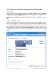
5.5.2 Generating a grid for background road sources
When filling in the menu Background Grid Emissions - Step 1 you are required
to have a shapefile with a grid for background road sources. You can generate such a file by using the SELMAGIS tool bar. Choose Domain > Terrain Create, and you will be presented with the dialog box shown in Figure 5.11.
Figure 5.11. Dialog box for creating terrain grid. Mesh size is filled in with 1000 m.
It is possible to define a grid shapefile by selecting a rectangle on the map
displayed in ArcMap or by defining the centre of the grid and give the
height and width extent. In any case the mesh size has to be defined. Here,
we outline the approach with creation of a grid rectangle. Further explanation can be found in the SELMAGIS help text, topic Terrain Grid. The help text
can be accessed through the SELMAGIS-dropdown menu on the SELMAGIS
toolbar.
In the dialog specify a Mesh size (e.g. 1,000 m). Press the X,Y button (marked
with a red rectangle in Figure 5.11). You should then see the tiny toolbar
shown in Figure 5.12, which allows you to draw and move a grid.
Figure 5.12. A click on the arrow icon on the tiny toolbar in the upper left corner (Selma
Terrain Factory) allows you to draw a grid.
If you press the Shift key while you draw the grid it will snap to rounded
coordinates corresponding to the mesh size. Finally, in the field Grid Shape
30
specify a file name, using the button to the right. Click OK in order to generate the grid file.
Note that with a standard installation a grid size of 1,000 m is required by
default. It is possible to use another grid size, but in that case you need to
change a setting in the configuration file Selmagis.ini – see the Appendix,
section 7.4.
5.5.3 Background Grid Emissions - Step 2
In this step a file of the type *.arb ("ARea Background") is created.
Figure 5.13. Background Grid Emissions, Step 2. When you encounter this window, the
uppermost file name (the *.mdb Traffic Category file) will typically be filled in because it
was created during Step 1. The subsequent fields must be filled in as explained below.
To the right of each field are two icons: the leftmost is for browsing to the file, while the
rightmost is for inspecting the file with suitable software.
Similar to the procedure for target roads it is required that you have access
to certain files which are typically created with OSPM tools. With a default
installation you can find samples as indicated in the following. Two files are
required:
 An OSPM Vehicle List file (*.vlf). With a default installation you may as
an example indicate the file
C:\Apps\Winospm\Lists\National\DK\VehiclesDK12_2013mil.vlf
 An OSPM Fuel List file (*.flf). With a default installation you may as an
example indicate the file
C:\Apps\Winospm\Lists\National\DK\Fuels_1999_El_FC_PN.flf
There are more details on the contents of these files in the OSPM manual.
The outcome of Step 2 is an *.arb ("ARea Background") file. You must specify
a name for it in the last field of the window in Figure 5.13. The *.arb file is a
text file used by OML-Highway; it provides information on gridded emission from background roads.
Press the Start button, and after a successful run you can close the window
and confirm that you wish to add the *.arb file to the current project.
31
In addition to the *.arb file, a *.deb ("Diurnal Emissions Background") file is
required for OML-Highway to run. This is a file somewhat similar to the
*.det file that contains information on the diurnal variation of emissions
from the target roads, but the *.deb file concerns background roads and relative diurnal emission factors. The file contains diurnal emission profiles that
are normalized to 1 for all pollutants. There is no tool in SELMA GIS to produce this file. If data for the area of interest are available the user can create
this file manually. Otherwise, the sample *.deb file provided with the installation package can be used if seen appropriate for the region. Typically, a
precise description of the diurnal variation of emissions for background
roads will be less important than the diurnal variation for target roads, and
therefore use of the sample file will be acceptable.
The sample *.deb file is located as
VariousOML_files\BackgroundDiurnalEmissions.deb. The *.arb and *.deb
files can be inspected by pressing the rightmost icon besides the name of the
file (see Figure 5.14).
Figure 5.14. OML-Highway Navigator window after an *.arb file has been created and a
*.deb file specified.
5.6
Emissions - Other Background Emissions
In the third and last dialog to create emission input files you can specify the
data for other background emissions (an *.aro file) and create a shapefile
from your *.aro file. If you don’t have any important background sources
other than traffic you can skip this step. However, you must make sure to
remove the checkmark, which may be set at “Select Other Background Emissions” (if you don’t, you won’t be able to run the OML-Highway model in
the last step).
There is an example of an *.aro file in the sample data set, as
VariousOML_files\OtherBackgroundSources.aro
32
Figure 5.15. You can use this menu if you wish to take other background emissions than
road sources into account. If you don’t want this you should make sure to deselect the
check mark on top (“Select Other Background Emissions”).
5.7
Receptors
Concentrations are calculated in receptor points, the location of which can be
specified by the model user. OML-Highway Navigator offers to assist with
preparation of files concerning receptor points.
You can access these tools from OML-Highway Navigator by selecting the
label Receptors and clicking the button Create Receptor File. As an alternative,
you can use the SELMAGIS toolbar and select Domain > Receptors OML.
This leads to the window shown in Figure 5.16.
33
Figure 5.16. Tools for creating receptor points. The tab Along roads is selected and partly
filled in. To the right the result is illustrated: Receptor points are distributed along target
roads. They are situated in 'perpendiculars' (series perpendicular to the road) with a distance of 400 meters (“perpendicular distance”) and extending to a distance of 150 meters
from the road. The “Offset for perpendicular distances” can be set to 0, unless you wish to
move the set of receptors a certain distance along the road.
There are four tabs, corresponding to four methods to create or import receptor points.
5.7.1 Receptors along roads
An often used tool allows the user to generate receptor points along target
roads, at various distances from the road. Figure 5.16 shows the tab corresponding to this tool. The top part of the menu is filled in, allowing receptor
points to be created.
First, a road shapefile is specified. Next, "perpendiculars" with series of receptor points are defined as illustrated in Figure 5.16.
The parameter of default terrain height is mandatory although it only matters if you are particularly concerned about high bridges (elevated points).
In all other cases the emission will follow the local orography.
The “receptor height” is the height (above the ground) where concentrations
are considered. Often a height of 1.5 m or 2 m is used.
The user must specify the name of a shapefile to contain the generated receptor points. This is done by pressing the button next to the file name field.
34
When all fields above the button Create Receptorpoints have been filled in, the
button can be pressed and a shapefile thereby generated.
This shapefile is not sufficient as input to OML-Highway; OML-Highway
needs a receptor file in *.rct format. For this purpose the bottom part of the
menu in Figure 5.16 must be filled in. The largest terrain inclination in the
area must be specified, as well as the general roughness length of the area.
The roughness length depends on land cover. Often, a value of 0.1 m is used
in the countryside and 0.3 m in urban areas. There is a drop-down menu to
assist in the selection. Note that there is an option (-1) to indicate that you
will just use the roughness length from the meteorological data file. In the
help text of SELMAGIS there is a table indicating examples of land cover and
roughness values. The end results in terms of concentrations are normally
not very sensitive to the values chosen for terrain inclination and roughness
length.
For the advanced user it can be of interest to know that the drop-down list
with roughness values is defined in the initialization file SelmaGIS.ini (more
information in the Appendix section 7.4)
At the bottom of the menu the user must specify the name of an *.rct file
(OML receptor file). This must be done making use of the button just to the
right of field. When the name has been specified (and provided that a receptor shapefile has already been created), the button Convert to *.rct can be
pressed.
The receptor point menu contains the option “Create line”. This is a facility
which can be useful for presentation purposes. It is explained in more detail
in section 5.7.5.
5.7.2 Receptors in a background source grid
The menu shown in Figure 5.16 has four tabs, corresponding to four methods to create or import receptor points. The second tab “Background” allows
the user to create receptor points based on a background source grid (the
creation of such a grid was discussed in Section 5.5). One receptor point will
be created in the centre of each grid cell.
5.7.3 Import of existing OML receptor file
The third tab in the menu shown in Figure 5.16 can be used for the situation,
where the user has an OML receptor file (*.rct), but not a corresponding
shapefile, and wishes to create one. By default “Use parameters from input
file” is checked, implying that values for receptor and terrain height are taken from the OML receptor file.
This import option is also useful if you have several *.rct files, which you
wish to combine. You can then take a detour via shapefiles, which you create
here, and subsequently import using the fourth tab (explained next).
35
5.7.4 Import of receptor point shapefile
The fourth tab in the menu shown in Figure 5.16 can be used to convert a receptor point shapefile to an OML receptor file (*.rct). If you have several
shapefiles you can combine them by checking the option “Append Receptors” for the second and later files when you create a combined shapefile.
Finally, you can convert this shapefile to an OML receptor file.
5.7.5 Creating buffer zones for presentation purposes
Above, basic information concerning creation of receptor points is given. By
applying ArcMap tools there are various ways to present model results. The
left part of Figure 5.17 shows how symbols in receptor points can be colourcoded to visualise concentrations. If you want a smoother visualization like
the one on the right with buffer zones you can make use of the option “Create line” in the receptor point menu and subsequently apply various
ArcMap tools. This involves an alternative way of creating receptor points.
The procedure is explained in the following; it may appear complicated, so
you may choose to read it only when you need it.
Figure 5.17. Visualisation of OML-Highway results (concentrations). On the left symbols in
receptor points are colour-coded. On the right a procedure with creation of buffer zones
has been used. Here, a receptor has been placed in the middle of each buffer zone (see
text).
In Figure 5.18 (left) the menu for receptors along roads has been filled in
with values of 20 m and 2,020 m for perpendiculars, and the “Create line”
option has been checked. This implies that the button “Create Receptors”
has been replaced by a button named “Create Lines”. The result of using it is
shown on the right in the figure: Lines are drawn perpendicular to the road,
between points 20 m and 2,020 m from the road on each side (due to the
scale in the figure no gaps at the road are visible). The distance between the
lines is 1000 m; an offset of 500 m has been specified, but this is unimportant
– it just moves the entire set of lines 500 m along the road (compared to 0).
36
Figure 5.18. Using the menu for receptors to create lines perpendicular to target roads.
These lines are used in a subsequent process, where polygons are created with ArcMap
tools.
Next, you can use the ArcMap tool Multiple Ring Buffer tool located under
Analysis Tools/Proximity to create buffers around the target roads. You can
define the number of buffers at each side of the road located and the distance between them.
By using the Split Polygons tool located under the Topography tool and using
the previously created lines, this buffer zone is then cut into n continuous
polygons along the road network, where n denotes the number of receptor
points on each side of the road. Next, by using the Multipart to Singlepart tool
located under Data Management/Features the polygons can be further split
into individual smaller polygons, each representing a polygon around each
receptor that you wish to create on each side of the road network.
Figure 5.19. Buffers along target roads and receptor points placed within them.
Further, create a shapefile with receptor points in the centre of each polygon
(using the tool Data Management > Feature to point) as illustrated in Figure
5.19. This shapefile is used as input to the fourth tab in the receptor point
menus (section 5.7.4) to create an *.rct file for OML-Highway.
37
After running OML-Highway you can join a shapefile containing results to
the receptor file with polygons, using proximity as a criterion for the join.
With the resulting file you can visualize results to get an output similar to
the right part of Figure 5.17.
5.8
Background concentrations
OML-Highway can make calculations of air pollution concentrations based
on the emissions provided in the previous steps. However, there is additional air pollution that has to be taken into account, namely regional background concentrations. This concentration contribution is the result of emissions from other sources than those explicitly specified, typically from
sources outside the domain considered.
Some air pollutants – such as CO – are simply additive, in the sense that total concentration can be found by adding background values and local concentration contributions. However, for others, in particular NO2, NO and
ozone, there is an interaction involving chemical reactions, so their level can
only be correctly determined if background concentrations are taken into account.
Therefore, the user should by some means acquire hourly data for the background concentration of a number of air pollution components and provide
them as input for OML-Highway. For instance, there may be available observational data available from a rural monitoring station or from a regional
air quality model. The structure of the file with background concentration
data (a *.dat file) is described in the appendix, section 7.3.6. The pollutants in
the file are NOX, NO2, O3, CO, CO2, PM2.5, PM10 and particle number. If, e.g.,
CO2 is not of interest the values can be indicated as a negative number,
meaning that data are missing. As mentioned above, you should make efforts to have reasonable values for NO2, NO and ozone, as chemical reactions
will otherwise not be taken correctly into account. Details on treatment of
missing values can be found in the appendix, section 7.3.6.
There is a sample of such a data set as
TestData\VariousOML_files\RegionalBackgroundConc.dat
Figure 5.20. OML-Highway Navigator. Dialogue where a file with background concentration data is included in the SELMAGIS project.
38
5.9
Meteorology
The meteorological data used for OML-Highway is a time series for one
point, which represents meteorological conditions in the entire modelling
area. In OML-Highway you can either use your own tools to produce a *.met
file in the correct format (*.met), or you can supply meteorology data in the
form of a *.txt file, from which a *.met file is generated with a meteorological
preprocessor. Such a preprocessor is accessible by using the button “Create
OML meteorological file” in Figure 5.21.
The first option where you provide a ready-made *.met file require that you
have access to certain advanced parameters (e.g. friction velocity and mixing
height), not just those directly observed at ordinary meteorological stations.
This can be obtained by using a meteorological model and applying appropriate post-processing. There is further information on the contents and
structure of *.met files in the Appendix, Section 7.3.7.
Figure 5.21. OML-Highway Navigator. The menu where the meteorological file is specified. Note the third button next to the field with the name of the *.met file. This button gives
access to a wind rose based on the meteorological data file.
In Figure 5.21 the meteorological file specified is taken from the sample
package: TestData\VariousOML_files\Meteorology.met
These data were generated with the MM5 meteorological model and subsequently post-processed.
By pressing “Create OML meteorological file” the user gets the opportunity
to create data according to the second option mentioned above, where the
user supplies a *.txt file with wind speed, temperature and various other information, and subsequently can run a meteorological preprocessor to create
the data file. There is a sample file for this purpose in TestData\VariousOML_files\Kastrup_2005_SynopticMet.txt, and an explanation of the file in the Appendix, section 7.3.8.
39
5.10 Run OML-Highway
To run the calculations and analysis of OML-Highway you should proceed
to the last label in OML-Highway Navigator: “Run OML-Highway” as
shown in Figure 5.22.
Here you should specify the calculation period and the name and location
for the output file. For the sample data, the relevant year is 2009, as the
background concentrations and the file Meteorology.met refer to that year.
You can only start a calculation if there are green checkmarks at all previous
steps in the process (with the possible exception of “Other Background”). If
the button to start the calculation isn’t active, you should check your specifications concerning “Other Background“ emissions. In that menu, you must
make sure to remove the checkmark, which may be set at “Select Other
Background Emissions” (Figure 5.15).
OML-Highway makes calculations for each hour in the calculation period.
Output files are divided into two groups: statistics and time series. For each
run of OML-Highway seven files with statistics are produced. These are,
e.g., average values for the calculation period, and the maximum of hourly
values for the calculation period. Further, a log file with the same name as
the statistics is produced. More information on statistics files is found in the
Appendix, Section 7.3.9.
As a user you should specify a file name for files with statistics without indicating any extension. During the OML-Highway run the seven statistics files
are created. They bear different extensions, thus allowing you to identify
their content. In addition, a log is produced in a file with extension *.log.
The second “group” of output files consists of one file only: An *.out file,
which contains a time series of concentrations for receptors according to
your specifications. This specification is given by an attribute in the receptor
file: If the field RFTIMES is 1 (instead of 0) an hourly series of concentrations
for that receptor is included in the *.out file. The format of an *.out file is described in the Appendix, Section 7.3.10.
40
Figure 5.22. OML-Highway Navigator. Dialogue to run OML-Highway.
You start a run by pressing the button Run OML-Highway.
After the run you are asked whether you wish to see the log file. The log file
gives an overview of input data and contains summary tables of results. It is
located in the same folder as the files with statistics.
Subsequently, you may choose “View results”. This is the step to take if you
wish to visualize the results in ArcMap. In the window that appears (Figure
5.23) you should specify location and name for the result files which have
been produced (just point to an arbitrary file among those with statistics),
and for a shapefile with results to be produced. Then press Start.
A shapefile will be produced, containing statistics for the various components (PM2.5, NO2 etc.) and parameters (annual average, 19th highest hourly
value, etc.). See the Appendix, section 7.3.9 for further details.
Subsequently you can use ArcMap to visualize the results, e.g. by colourcoding concentrations values in the receptor points as illustrated in Figure
5.24.
Figure 5.23. Dialogue to process results for viewing them as a shapefile.
41
Figure 5.24. Setting colour-coding for visualisation of mean value of PM2.5.
5.10.1 Exporting inputs
The menu in Figure 5.22 gives you the option to export all input files, so they
can be run on another PC. You may also wish just to export the input to another folder in order to get less clutter with a large number of files in the
folder where you currently work.
Choosing the export option means that all necessary input files for an OMLHighway run are copied to a single folder (with flat structure). A run can be
performed by creating a .bat file with a content of a single line in that folder,
and subsequently executing it. The contents of the .bat file should be:
c:\apps\selmagis\omlhw\OML-hw.exe OML-Highway.ini /Wl,Rm:Error-OML.txt
provided the export folder is on a PC with an OML-Highway installation.
Otherwise, you can copy the OML-Highway executable to the folder and
simplify the .bat file to
OML-hw.exe OML-Highway.ini /Wl,Rm:Error-OML.txt
The executable can be found as C:\Apps\SelmaGis\OMLHW\OML-hw.exe
5.11 SELMAGIS toolbar – remaining items
Figure 5.25. SELMAGIS toolbar. The toolbar can be floating or docked. If docked, the left
edge is a handle that can be used to move the toolbar.
In the preceding sections, focus has been on two of the items on SELMA GIS
toolbar, namely the SELMAGIS menu and the OML-Highway Navigator button.
There are several remaining items on the toolbar. However, nearly all of
these offer just an alternative way of accessing the dialogs that are described
in relation to OML-Highway Navigator.
42
The only exceptions are:
 Visualisation of noise barriers via the menu item Results
 The menu item Digitizing that enables the user to edit certain features of
the road network (presence of noise barrier) and of receptor points (receptor height, terrain height, and whether a time series of concentrations
for the receptor point should be saved).
Visualisation of noise barriers is described in the next section.
For help on the Digitizing menu, consult the SELMAGIS help (section 5.2 explains how to access the help).
5.11.1 Results - Visualisation of noise barriers
From the Results menu you can choose “Visualise Noise Barriers”. This is
only relevant if your Road Network Shapefile contains data that specify
noise barriers.
These data are indicated in two fields of the input road network shapefile.
They are: NDistance and NSide. A description of these parameters is given
in the Appendix, Table 7.2.
43
6
References
Berger, J., Walker, S. E., Denby, B., Berkowicz, R., Løfstrøm, P., Ketzel, M.,
Härkönen, J.,Nikmo, J. and Karppinen, A., 2010: Evaluation and intercomparison of open road line source models currently in use in the Nordic
countries, Boreal Env. Res., 15.
Berkowicz, R., 2000: OSPM – A parameterised street pollution model. Environmental Monitoring and Assessment 65 (1/2), 323–331.
Berkowicz, R., Olesen, H.R., Jensen, S.S., 2003: User’s Guide to WinOSPM
(OSPM User’s Guide). Comes with an installation of WinOSPM and can be
opened from the Help menu in WinOSPM.
Jensen, S. S., Løfstrøm, P., Berkowicz, R., Olesen, H.R., Frydendall, J., Fuglsang, K, and Hummelshøj, P. 2004: Air Quality Along Motorways – Measurement Campaign and Model Calculations. National Environmental Research Institute. NERI Technical Report No. 522. (In Danish with English
summary).
Jensen, S.S., Hvidberg, M., Petersen, J., Storm, L., Stausgaard, L., Becker, T.,
Hertel, O., 2008: GIS-baseret national vej- og trafikdatabase 1960-2005. Danmarks Miljøundersøgelser, Aarhus Universitet. 74 s – Faglig rapport fra
DMU nr. 678. http://www.dmu.dk/FR678.pdf.
Jensen, S. S., Becker, T., Ketzel, M., Løfstrøm, P., Olesen, H.R. and Lorentz,
H. 2010: OML-Highway within the framework of SELMAGIS. Final Report.
National Environmental Research Institute, Aarhus University, Denmark, 26
pp, NERI Technical Report No. 771. http://www.dmu.dk/Pub/FR771.pdf.
Jensen, S.S., Ketzel, M., Becker, T., Løfstrøm, P., Olesen, H.R., Lorentz, H.,
Nøhr Michelsen, L, Fryd, J. 2010: OML-Highway - en ny brugervenlig GISbaseret luftkvalitetsmodel for veje i åbent terræn. In: Trafik og Veje, Vol. 10,
2010, p. 34-36.
Jensen, S.S., Ketzel, M., Becker, T., Hertel, O., Løfstrøm, P., Olesen, H.R.
2011: Air Quality Assessment of Alternatives for a New Crossing of the Inlet
of Limfjorden. EIA, National Environmental Research Institute, Aarhus University. 86 p. – Report No. 824. http://www.dmu.dk/Pub/FR824.pdf (In
Danish).
Jensen, S.S., Ketzel, M., Hertel, O., Becker, T. 2011: Luftkvalitetsvurdering for
rute 26 Viborg - Aarhus : VVM redegørelse. Aarhus University, DCE – Danish Centre for Environment and Energy, 72 pp. Scientific Report from DCE –
Danish Centre for Environment and Energy No. 12,
http://dce2.au.dk/pub/SR12.pdf
Jensen, S.S., Ketzel, M., Becker, T., Løfstrøm, P., Olesen, H.R., 2011: Luftkvalitetsvurdering for udvidelse af motorvej syd om Odense : VVM redegørelse.
Danmarks Miljøundersøgelser, Aarhus Universitet, 2011. 56 s. (Faglig rapport fra DMU; Nr. 825).
44
Jensen, S.S., Ketzel, M., Becker, T., Løfstrøm, P., Hertel, O., Olesen, H.R., Lorentz, H. 2012: OML-Highway - A GIS-based road source model for air quality assessment – applications in EIA. Proceedings of Abstracts. 8th International Conference on Air Quality - Science and Application. red. / Vikas
Singh; Heather Price; John Bartzis; Ranjeet S. Sokhi. University of Hertfordshire Press, 2012. s. 81.
Jensen, S.S., Ketzel, M., Hertel, O., Becker, T., Løfstrøm, P., Olesen, H.R.
2013: Vejledning i luftkvalitetsvurdering af motorveje. Aarhus Universitet,
DCE – Nationalt Center for Miljø og Energi. Vejdirektoratet, rapport 455 –
2013.
http://www.vejdirektoratet.dk/DA/viden_og_data/publikationer/Lists/P
ublikationer/Attachments/831/Luftkvalitetsvurdering_rap455.pdf
Jensen, S.S., Im, U., Ketzel, M., Løfstrøm, P., Brandt, J. 2015: Mapping of air
quality along motorways and other main roads in Denmark (in Danish with
English summary). Aarhus University. Scientific Report from DCE – Danish
Centre for Environment and Energy No. 154
http://dce2.au.dk/pub/SR154.pdf
Olesen, H.R., Berkowicz, R.B, Løfstrøm, P., 2007: OML: Review of model
formulation. National Environmental Research Institute, Denmark. 130pp. NERI Technical Report No. 609, http://www.dmu.dk/Pub/FR609.
Wang, F., Ketzel, M., Ellermann, T., Wåhlin, P., Jensen, S. S., Fang, D., and
Massling, A. , 2010. Particle number, particle mass and NOx emission factors
at a highway and an urban street in Copenhagen, Atmos. Chem. Phys., 10,
2745-2764.
45
7
Appendix
This appendix contains the following sections:






Conventions
Guide to file extensions
Description of input files
o Road network shapefile (RNS)
o *.art – ARea Target
o *.det – Diurnal Emission Variation
o *.arb – ARea Background
o *.deb – Diurnal Emissions Background
o *.dat – regional background concentrations
o *.met – meteorological input
o *.txt – meteorological input to be preprocessed
o output files with statistics
o *.out – time series of calculated concentrations
Configuration file SelmaGIS.ini
Description of sample data
Definition of “day case”
Note that section 7.2 “Guide to file extensions” is very useful as a reference.
7.1
Conventions
Time format: values 1-24 indicate the end of the hour for which averages are
given.
In data files in text format OML-Highway uses as decimal separator a “.”
(period). This should also be the system setting when working with OMLHighway.
SELMAGIS versions distributed prior to November 15, 2014 produce files
where the variable IDTRAFCCAT is named IDDIURNAL (this is a setting in
the configuration file SelmaGIS.ini).
In the description given in the present user guide we assume that SELMAGIS
has been installed in folder C:\Apps\SELMAGIS and WinOSPM in folder
C:\Apps\WinOSPM.
46
7.2
Guide to file extensions
Table 7.1. Guide to file extensions (continued on next page).
Extension
Mnemonic
Explanation
Produced by
arb
Area Road
Text file with gridded information on emission from background roads. SELMAGIS
Background
Does not include information on variation with time. See Appendix,
section 7.3.4 for a description.
aro
art
ARea Other
ARea Target
Optional text file for providing information on other background
The user; no tool availa-
sources than roads.
ble.
Text file to provide information on all target road segments, the
SELMAGIS
amount of traffic they carry, and Traffic Composition ID. Does not
include information on variation with time. See Appendix, section
7.3.2 for a description.
dat
deb
Text file to provide information on regional background concentra-
The user; no tool availa-
tions. See Appendix, section 7.3.6 for a description.
ble.
Diurnal
Text file resembling a *.det file, see below; however, a *.deb file re-
The user; no tool availa-
Emissions
fers to background road emissions. A sample is provided, which may ble.
Background
be acceptable for direct use. See Appendix, section 7.3.5 for a description.
det
Diurnal
Text file, "Diurnal Emission Variation File". Information on the time
Emission
variation of emissions from target road sources. There is a group of
SELMAGIS
variation for Tar- lines for each Traffic Composition Category. Within each such group,
get roads
there is a line for each hour of day and each "day case" (defined in
appendix,
Table 7.11), i.e. 24 x 8 = 192 lines. The table of emissions is normalized to an AADT of 10,000. See Appendix, section 7.3.3 for a description.
emi
Text file with annual emissions for each segment of the target roads. SELMAGIS
The name includes the string "RSC" (Road Source Characteristics)
flf
Fuel List File
Text file in format developed for WinOSPM. Contains pointers to
WinOSPM
other files with data on the fuel composition, as well as expressions
used for calculation of the emission factors. See OSPM manual for
explanation.
H19HrM
Statics; output from OML-Highway run.
OML-Highway run
H26D8hr
Statics; output from OML-Highway run.
OML-Highway run
H36DayM
Statics; output from OML-Highway run.
OML-Highway run
H8DayM
Statics; output from OML-Highway run.
OML-Highway run
ini
SelmaGIS.ini is a text file with configuration parameters for SEL-
Intrinsic
MAGIS. Located in the same folder as the SELMAGIS executable.
The user should normally not change this file. See Appendix, section
7.4 for a description.
log
Log. Running OML-Highway produces a log file.
OML-Highway run
Max1hr
Statics; output from OML-Highway run.
OML-Highway run
Max8hr
Statics; output from OML-Highway run.
OML-Highway run
47
Table 7.1. (continued) Guide to file extensions.
Extension
Mnemonic
mdb
Explanation
Produced by
Access data base with kilometers travelled in each background grid
SELMAGIS
cell. There are data for each of five background road types.
mean
Statics; output from OML-Highway run.
OML-Highway run
met
Meteorological file in format appropriate for OML-Highway.
SELMAGIS or External
mxd
ArcMap project.
ArcMap
out
Output from OML-Highway run in the form of a time series of concen-
OML-Highway run
tration values for selected receptors.
prj
Information on geographic projection.
SELMAGIS
rct
ReCepTor
Receptor data.
SELMAGIS
sel
SELMAGIS
SELMAGIS project file.
Intrinsic
shp, BSF
Background Sources Shapefile (BSF).
SELMAGIS
shp, GBS
Grid for Background Sources Shapefile (GBS).
SELMAGIS
shp, RNS
Road Network File Road Network Shapefile (RNS).
External
shp, RSC
Road Source
Road Source Characteristics Shapefile (RSC).
SELMAGIS
shp, RSC
Road Emission Shapefile (RSC).
SELMAGIS
shp, RSF
Receptor Characteristics Shapefile (RSF).
SELMAGIS
Characteristics
trf
Traffic
Diurnal Traffic variation file, e.g. Type_A.trf. Described to some extent WinOSPM
in section 2.4; more detailed explanation in OSPM manual.
txt
Used for meteorological input to be treated by met. preprocessor. See WinOSPM
Appendix, section 7.3.8 for a description.
vlf
Vehicle List File
Text file in format developed for WinOSPM. Contains pointers to other WinOSPM
files, which actually contain data used for calculations of emission
factors. See OSPM manual for explanation.
xls
48
Used for Traffic Composition Category file.
SELMAGIS
7.3
Description of input files
7.3.1 Road network shapefile
A network shapefile contains characteristics of either target roads, background roads, or both types of roads. The field Tflag indicates the type of the
road. This file must be constructed by the user before running OMLHighway. However, the two last parameters in the table (Nside and IDTRAFCCAT) are calculated by SELMAGIS.
Table 7.2. Definition of fields in the road network shapefile. The column Target/Background indicates whether the parameter is
relevant for Target roads, Background roads or both.
Fieldname
Data description
Target/Background
Format
Shape
RoadID
Polyline
Both
Geometry
Unique number
Both
Roadtype
ID for road type used for background roads to characterise their traffic
Integer
Background
Integer
Target
Integer
Both
Float/Double
Background
Float/Double
Background
Float/Double
Background
Float/Double
Background
Float/Double
Target
Float/Double
Target
Text
Target
Float/Double
Both
Integer
conditions. Five types are used (2111, 2112...), see section 2.6.
DoubleD
Double digitized = 2, otherwise = 1. For double digitized roads there are
two close, approximately parallel road segments, each of which carries
traffic in one direction. In chapter 2 on concepts this is further explained.
AADT
Annual Average Daily Traffic (number)
FPass
Fraction of passenger cars. Number between 0 and 1. The sum
(FPass+FVans+FTrucks+FBus) should be 1.
FVans
Fraction of vans. Number between 0 and 1. The sum
(FPass+FVans+FTrucks+FBus) should be 1.
FTrucks
Fraction of trucks. Number between 0 and 1. The sum
(FPass+FVans+FTrucks+FBus) should be 1.
FBus
Fraction of buses. Number between 0 and 1. The sum
(FPass+FVans+FTrucks+FBus) should be 1.
FHeavyDuty
Fraction in percent of heavy duty vehicles (sum of trucks and buses, but
in percent).
OSPMType
Id for traffic type used for target roads to characterise their traffic conditions. An example is Type A.trf, which is a standard OSPM diurnal type.
This is discussed in chapter 2 on concepts.
Roadwidth
Width of carriageway of road segment (m); if double digitized only one
direction.
SpeedLight
Speed of light traffic in km/h. This speed is a scaling speed which implicitly defines the speed of heavy traffic. The speed for an actual hour may
be different and is computed based on information in *.trf files.
DamH
Height of dam (positive) or cutting (negative) in relation to ground (m)
Target
Float/Double
WallH
Height of noise wall (m).
Target
Float/Double
EmbankH
Height of embankment (m).
Target
Float/Double
TFlag
Flag. 1 for target roads, 2 for background roads; records with other
Both
Integer
values are ignored.
NDistance
Distance from road centre line to noise wall/embankment (m).
Target
Integer
NSide
Location of noise barrier in relation to the road follows the convention of
Target
Integer
Target
Integer
OSPM (either 1 or 2); created by SELMAGIS.
IDTRAFCCAT Id for traffic composition categories; created by SELMAGIS. Note that
SELMAGIS versions distributed prior to November 15, 2014 produce files
where the variable IDTRAFCCAT is named IDDIURNAL.
49
...
....
Figure 7.1. Sample of shapefile. The number of parameters is large, so a snapshot of the file has been divided into a left part
(on top) and a right part (below it). The sample contains more information than the required minimum.
7.3.2 Files of type *.art – ARea Target
An *.art file is a text file used by OML-Highway to provide information on
all target road segments and the traffic they carry.
Table 7.3. Data structure of the *.art file (“ARea Target”). This is a text file with a 6-line header. Figure 7.2 shows a sample. This
table describes the parameters in the body of the file.
Field name
Data description
ID
Source ID (for the road segment). A unique number. Called SOURCEID in RSC shapefile.
X
X-coordinate of the south west corner of the area source segment.
Y
Y-coordinate of the south west corner of the area source segment.
L1
Length of the first side of the area source when moving clockwise from southwest corner.
L2
Length of the second side. Max ratio L1/L2 for line sources is 1:10 (or 10:1).
TETA
Angle in degrees of L1 with respect to north values; 0-90 possible. Zero if L1 is North-South.
H_Rd
Height of the road/bridge in m.
H_DoC
Height of the dam/cutting in m.
AAdt
AADT annual average daily traffic in veh/day.
Id
Id for traffic composition categories, also referred to as IDTRAFCCAT in shapefiles.
Id
Source Id of the road segment in the opposite direction. Called OPPOSITEID in RSC shapefile.
Width
Total width over both directions. Called DOUBLWIDTH in RSC shapefile. Calculated by SELMAGIS.
Wall
Height of the noise barrier in m. Called WALLH in RSC shapefile.
Embankment
Height of the embankment in m. Called EMBANKH in RSC shapefile.
Figure 7.2. Sample of an *.art file. The sample shown has been reformatted slightly for legibility.
50
7.3.3 Files of type *.det – Diurnal Emission Variation
A "Diurnal Emission Variation File" is a text file providing information on
the time variation of emissions from target road sources. It is created by
SELMAGIS. There is a group of lines for each Traffic Composition Category.
Within each such group, there is a line for each hour of day and each "day
case", i.e. 24 x 8 = 192 lines. The table of emissions is normalized to an AADT
of 10,000. The definition of day cases is given in the Appendix, Section 7.6.
The file is used by OML-Highway as a lookup table for emissions.
Table 7.4. Data structure of the *.det file (“Diurnal Emission variation for Target roads”); emissions normalized to annual average daily traffic (AADT) of 10,000 vehicles
Fieldname
Data description
ID
ID for traffic composition category, also referred to as IDTRAFCCAT in shapefiles.
Weekday
Number of the day of the week; Monday = 1.
Mth
Number of the month; January = 1.
Day-Case
8 “day-cases” are defined, e.g. “Fridays in July”. Defined in the Appendix, Section 7.6.
Hr
Hour of the day; 1 – 24.
Nlight
Number of light vehicles during the hour considered.
Nheavy
Number of heavy duty vehicles during the hour considered.
Speed Vlight
Speed of light traffic in km/h.
Speed Vheavy
Speed of heavy duty traffic in km/h.
NOx
Emission in μg/m/s.
fractionNO2
Emission in %.
CO
Emission in μg/m/s.
CO2
Emission in μg/m/s.
PMexhaust
Emission in μg/m/s.
PM2.5
Emission in μg/m/s.
PM10
Emission in μg/m/s.
Pnumber
Particle number in #/m/s.
....
Figure 7.3. Sample of *.det file. ID in the first column refers to Traffic Composition Category. The file is wider than shown. The
sample shown has been reformatted slightly for legibility.
51
7.3.4 Files of type *.arb – ARea Background
A file of type *.arb is a text file, which describes cells with gridded emission
data. It concerns emission from background roads. Each record describes the
geometry and annual emission of one cell.
Table 7.5. Data structure of the *.arb file (“ARea Background”). This is a text file with a 6-line header.
Field name
Data description
ID
ID for background source. A unique number.
X
X-coordinate of the lower left corner of the area source.
Y
Y-coordinate of the lower left corner of the area source.
L1
Length of the first side of the area source when moving clockwise from southwest corner
L2
Length of the second side. Max ratio L1/L2 for line sources is 1:10 (or 10:1).
TETA
Angle in degrees of L1 with respect to North; values 0-90 possible. Zero if L1 is North-South
HS
Height of the release from background source in m. The default value is 1 m.
HB
Parameter with a default value of 3 m. Ensures a suitable initial dispersion for the area source,
taking traffic produced turbulence into account.
Id
ID of the traffic composition category for background roads. For background roads, only a value of
1 is currently used.
QNOx
Emissions in kg/year
fractionNO2
Emission fraction of NO2 in %.
QCO
Emissions in kg/ year.
QCO2
Emissions in kg/ year.
QPMExh
Emissions in kg/ year.
QPM2.5
Emissions in kg/ year.
QPM10
Emissions in kg/ year.
QPNumber
Particle number in 1014#/ year.
Number and order of parameters/components are fixed. (Line no. 1-6 are not read.
Missing emission values are negative.
Traffic
compos.
(-)
(m)
(m)
(m) (m)(deg)(m) (m)catogory(kg/year (%)
(kg/year)
(kg/year)
(kg/year) (kg/year) (kg/year) (10^14#/yr)
ID
X
Y
L1 L2 TETA HS
HB Id
QNOX
fractionNO2
QCO
QCO2
QPMExh
QPM2.5
QPM10
QPNumber
1 570700 6129800 1000 1000 0 1.0 4.0 1
360.4322 24.13512 789.705 155966.531449219
7.246446 20.8284
52.53595 309654.4
2 571700 6129800 1000 1000 0 1.0 4.0 1
96.42887 21.59819 329.0174 49854.6120634766 2.171314 6.349024 15.58568 72151.63
3 572700 6129800 1000 1000 0 1.0 4.0 1
295.5294 24.24422 618.3944 125872.345769531 5.884074 16.88584 42.6975 256538.6
4 573700 6129800 1000 1000 0 1.0 4.0 1
211.6069 24.13281 464.0358 91594.7706171875 4.255135 12.23087 30.84874 181758.8
5 574700 6129800 1000 1000 0 1.0 4.0 1
201.263
22.70435 599.8583 98059.1344921875 4.360292 12.67854 31.40097 158479.8
Figure 7.4. Sample of an *.arb file. The sample shown has been reformatted slightly for legibility.
52
7.3.5 Files of type *.deb – Diurnal Emissions Background
A "Diurnal Emission Background file" is a text file. It provides information
on the diurnal variation of emissions from the background roads. The file
contains diurnal emission profiles that are normalized to 1 for all pollutants.
There is no tool in SELMAGIS to produce this file. If data for the area of interest are available the user can create this file manually. Otherwise, the sample
*.deb file provided with the installation package can be used if seen appropriate for the region. Typically, a precise description of the diurnal variation
of emissions for background roads will be less important than the diurnal
variation for target roads, and therefore use of the sample file will be acceptable.
Table 7.6. Data structure of the *.deb file (”Diurnal Emissions Background”).
Fieldname
Data description
ID
Id of the traffic composition category for background roads. For
background roads, only a value of 1 is currently used in the
calculations (a value of 2 appears in the sample file, but is not
used).
Weekday
Number for the day of the week; Monday = 1
Mth
Number of the month; January = 1
Day-Case
8 “day-cases” are defined, e.g. “Fridays in July”. Defined in the
Appendix, Section 7.6.
Hr
Hour of the day; 1 - 24
QNOx
Relative diurnal emission factors: daily average = 1
fractionNO2
Relative diurnal emission factors: daily average = 1
QCO
Relative diurnal emission factors: daily average = 1
QCO2
Relative diurnal emission factors: daily average = 1
QPM2.5
Relative diurnal emission factors: daily average = 1
QPM10
Relative diurnal emission factors: daily average = 1
QPnumber
Relative diurnal emission factors: daily average = 1
Figure 7.5. Sample of *.deb file. The sample shown is the one provided with an OML-Highway installation.
7.3.6 Files of type *.dat – regional background concentrations
Data for hourly values of regional background concentrations should be
provided in a text file with extension *.dat. Such data may have been acquired by monitoring or modelling.
Values are required for the following compounds: NOX, NO2, O3, CO, CO2,
PM2.5, PM10 and particle number. Missing values are indicated by negative
numbers. In the file, the order and number of parameters is fixed, but you
may for instance disregard a component by indicating missing values for all
hours.
53
Missing values (negative numbers) are handled in the following way:

If the first line in the file contains missing values for a component,
values for all subsequent hours for that component are assumed to
be missing.

If there are missing data later in the file the model “fills” the missing
data with the values from the previous valid hour. For longer periods of missing data (days, weeks) this might appear inappropriate
and the user should take care to remove these results in the output.

If one of the components NO2, NO and ozone is missing, all three
components are replaced with the previous complete valid set of
these components.
Table 7.7. Data structure of the *.dat file with regional background concentrations.
Fieldname
Data description
DATE
Date in format yyyymmdd
HR
Hour of the day; 1 - 24
NOX
Concentration as μg-NO2/m3
NO2
Concentration in μg/m3
O3
Concentration in μg/m3
CO
Concentration in μg/m3
CO2
Concentration in μg/m3
PM2.5
Concentration in μg/m3
PM10
Concentration in μg/m3
PNumber
Particle number in #/cm3
Figure 7.6. Sample of *.dat file with regional background concentrations.
7.3.7 Files of type *.met with meteorological input
A user of OML-Highway can either (1) supply meteorology data in the form
of a *.met file with ready-made data in the correct format, or (2) provide a
*.txt file, from which a *.met file is generated with a meteorological preprocessor built into OML-Highway.
Use of the first option requires that the user has access to certain advanced
parameters (e.g. friction velocity and mixing height), not just those directly
observed at ordinary meteorological stations. This can be obtained by using
a meteorological model and applying appropriate post-processing.
The first option can potentially yield data of higher quality than the second.
This is because the meteorological preprocessor is a simplistic special version of the OML meteorological preprocessor. It requires only synoptic data
(not radiosonde data), and it uses various simplifying assumptions, especially in calculation of mixing height.
54
This section gives the specifications for the *.met file used by the first option.
A sample of such a file is provided in the sample data set,
TestData\VariousOML_files\Meteorology.met
This approach requires that the user has access to certain advanced meteorological parameters (e.g. friction velocity and mixing height), not just those
directly observed at ordinary meteorological stations. This can be obtained
by using a meteorological model and applying appropriate post-processing.
The file contains hourly meteorological data. It has a 10-line header, followed by 8,760 (or 8,784) records for a full year’s worth of data. For the period with data the time series is expected to be complete without interruptions. The data structure of records is shown as Table 7.8 and the first lines
of the sample in Figure 7.7. More details are given after the figure.
Table 7.8. Data structure of records in a *.met file
Fieldname
Data description
DATE
Date in format yyyymmdd.
Hr
Hour in local standard time, 1-24 (end of averaging period).
AL
Monin-Obukhov length (m).
DD
Wind direction in degrees. 360 is North, while 0 is not allowed.
DELDD (or short: DLD)
Delta of the wind direction in degrees. Described in section 7.3.8.
HSTAR
Buoyancy heat flux in unit 0.001 m2/s3.
SZI
Stability parameter si for layer above zi in unit 0.001 s-2. -9.9999 for missing.
SZLID
Stability parameter si for layer above zlid in unit 0.001 s-2. -9.9999 for missing.
SZMIX
Stability parameter si for layer above zzmix in unit 0.001 s-2. -9.9999 for missing.
TT
Temperature (Kelvin).
UST
Friction velocity (m/s).
WST
Convective velocity (m/s).
ZI
Convective mixing height (m). -1 for missing.
ZLD
Height of “sustained lid” base (m). -1 for missing.
ZMIX
Operational mixing height (m).
Z0
Roughness length, m.
TD
Not used. You may e.g. indicate -1.
CLD
Not used. You may e.g. indicate -1.
RAD
Global radiation, W/m2.
Figure 7.7. The first lines of the sample file Meteorology.met with preprocessed meteorological input for OML-Highway in the
*.met format. Slightly reformatted for readability.The text in red is ignored by the program (comments for guidance).
The contents of the file is further specified below.
55
Values in a .met file are read using free format, i.e. they should be separated
by at least one blank, but it is unimportant whether they are in certain columns.
The file has a 10-line header. Figure 7.7 is useful as illustration. The text in
dark red is ignored by the program, but explains the parameters. The parameters in the header are:

Line 1: “Gis-format”. This keyword is mandatory for *.met input
files to be used by OML-Highway.

Line 2: STATION_NAME. Any name of your choice, max. 14 characters. Blanks are not permitted.

Line 3: The keyword “Coarse” or “Fine”. Use “Coarse” if the wind
direction is in tens of degrees, e.g. 10, 20 etc. If the measured wind
direction is indicated with a resolution of 1 degree, you should use
the keyword “Fine”. The wind direction should be given as integers,
no matter which keyword you use. If the option “Coarse” is used, a
random number function will be applied internally in OMLHighway to distribute wind directions evenly in ten degree intervals. For instance, instead of an indicated value of 10 a random value between 5 and 15 will be applied. If your data have different
resolution (e.g. 22.5 degrees), you must make your own preprocessing before supplying the data to OML-Highway.

Line 4: Three parameters should be given. First the latitude of the
met station; next the keyword “LST” (Local Standard Time) or
“GMT” depending on your convention when indicating time in the
meteorological file; and finally either the value 0.35 or 0.40. This
number is the value of the von Karman constant used when computing the various parameters. Files created with the OML preprocessor use a value of 0.35 for the von Karman constant, whereas e.g.
AERMOD uses 0.40.
Lines 5-10 are not read by OML-Highway, but can contain comments.
The records in line 11 onwards contain values of the various parameters. For
most parameters it is not permitted to have missing values, but for some a
missing value can be flagged as specified below. The list below provides
further explanation of certain variables:
56

HSTAR. The buoyancy heat flux HSTAR can be calculated from sensible heat flux at the surface (HF) by the equation
HSTAR = HF * g/(T * ϱ * cp)
where g is the gravitational acceleration, T the surface temperature
in Kelvin, ϱ the density of air, and cp the specific heat capacity of dry
air at constant pressure.
This amounts to approximately
HSTAR (m2/s3) = HF (W/m2)* 2.76 * 10-5 (m4/(Js2))
(however with temperature dependence).
In the OML input file the unit 0.001 m2/s3 is used for HSTAR, implying that e.g. a sensible heat flux of 100 W/m2 is indicated as (approximately) the value 2.76 in the OML input file.

Boundary layer height. OML uses a height of the convective boundary layer (ZI) and an operational mixing height (ZMIX), which may
be the same value. OML requires information about the lapse rate
(the stability parameter) in the layer above these two heights. Furthermore, the OML meteorological preprocessor uses the concept of
a “sustained lid” which may be present and limit mixing.
If you prepare your data by other means than the OML preprocessor you can flag the parameters relating to a sustained lid
(SZLID and ZLD) as missing. A missing value of ZI or ZLD is indicated as -1. Missing values of ZMIX are not permitted.

Stability parameter (SZI, SZLID and SZMIX). These parameters can
be computed from the lapse rate in the relevant layer as follows:
SZI (s-2) = γ * g/T
where γ is the potential temperature gradient in the layer (K/m), g
the gravitational acceleration (m/s-2), and T the temperature (K). SZI
refers to the layer above the convective mixing height, and SZMIX to
the layer above the operational mixing height. The value must be determined from available information. Missing values of either of the
stability parameters are allowed and are indicated as –9.9999.
In the OML input file the unit 0.001 s-2 is used for SZI etc., implying
that e.g. a potential temperature lapse rate of 10 K/km results in a
value of approximately 0.36 in the OML input file.

Convective velocity WST. This is a convective scaling velocity defined as (ZI * HSTAR)1/3 where ZI is the convective boundary layer
height. It is 0 m/s for night time conditions. In the OML preprocessor WST is computed for all daytime hours, based on the operational mixing height ZMIX when ZI is undefined.

RAD: Global radiation in W/m2. Global radiation is incoming solar
radiation, both directly from the sun and scattered by clouds. At
night its value is 0, during daytime its value is positive. RAD may be
missing. Indicate missing values as -99. In some contexts you may
encounter the name “GL” instead of RAD.
7.3.8 Files of type *.txt with meteorological input
A user of OML-Highway can either (1) supply meteorology data in the form
*.met file with ready-made data in the correct format, or (2) provide a *.txt
file, from which a *.met file is generated with a meteorological preprocessor
built into OML-Highway.
It should be noted that the meteorological preprocessor is a simplistic special
version of the OML meteorological preprocessor. It requires only synoptic
data (not radiosonde data), and it uses various simplifying assumptions, especially in calculation of mixing height. The first option where a user provides a ready-made *.met file can potentially yield data of higher quality.
This section gives the specifications for the *.txt file used by the second option.
A sample of such a file is provided in the sample data set,
TestData\VariousOML_files\Kastrup_2005_SynopticMet.txt
The file contains hourly meteorological data. It has a 10-line header, followed by 8760 (or 8784) records for a full year’s worth of data. For the period
with data the time series is expected to be complete without interruptions.
57
The data structure of records is shown as Table 7.9 and the first lines of the
sample in Figure 7.8. More details are given after the figure.
Table 7.9. Data structure of records in the *.txt file to be converted to *.met.
Fieldname
Data description
DATE
Date in format yyyymmdd.
Hr
Hour in local standard time, 1-24 (end of averaging period)
Cir
Indicates whether cirrus is the dominating cloud type. 0 or 1. Use 1 if cirrus is dominating, use 0 if it
isn’t, or if this information is missing.
DD
Wind direction in degrees. 360 is North, while 0 is not allowed.
DELDD
Delta of the wind direction in degrees.
QUAL
User-defined quality indicator.
FF
Wind speed in m/s.
HUM
Humidity in %.
NN
Cloud cover in eights (1-8).
RA
Indicates whether it has rained or not during previous hour (0 or 1, 0 for no rain).
SN
Indicates whether the ground is more than half covered with snow (0 or 1, 0 for no snow).
TC
Temperature in Celsius.
RAD
Global radiation, W/m2.
Z0
Estimated roughness length, m.
Figure 7.8. The first lines of the sample file Kastrup_2005_SynopticMet.txt, providing meteorological data to be used as input
for the met preprocessor in OML-Highway (its use is described in section 5.9).
The file has a 10-line header. In order to create your own file you should
copy the header in the example with the following changes:
58

Line 2: Replace “Kastrup” with a relevant station name. The name
should be no longer than 14 characters and must contain no spaces.

Line 3: The keyword “Coarse” or “Fine”. Use “Coarse” if the wind
direction is in tens of degrees, e.g. 10, 20 etc. If the measured wind
direction is indicated with a resolution of 1 degree, you should use
the keyword “Fine”. The wind direction should be given as integers,
no matter which keyword you use. If the option “Coarse” is used, a
random number function will be applied internally in OMLHighway to distribute wind directions evenly in ten degree intervals. For instance, instead of an indicated value of 10 a random value between 5 and 15 will be applied. If your data have different
resolution (e.g. 22.5 degrees), you must make your own preprocessing before supplying the data to OML-Highway.

Line 5: Replace Latitude, Anemometer height and Thermometer
height with relevant values. There should be at least one blank between parameters to separate them, but the exact position of the pa-
rameters doesn’t matter. You should leave Longitude and Timeshift
unchanged. Also leave other parameters in line 5 unchanged. The
convention for time units in the subsequent lines is that you should
use local standard time (not daylight saving time).
The records in line 11 onwards:

The values are read using free format, i.e. they should be separated
by at least one blank, but it is unimportant whether they are in columns.

In general it is not permitted to have missing values. Exceptions to
this rule are indicated where applicable. When you prepare data,
this requirement may sometimes force you to create data values by
some method (interpolation, copying from a previous hour or some
sort of random generator).

For CIR just indicate the value 0.

DELDD is the change in wind direction from one hour to the next
(based on wind direction for the previous, the current and the next
hour). The unit is degrees. Assuming that DD_after is the wind direction during the hour after the current, and DD_before the wind direction during the previous hour, DelDD can be computed by this
piece of code:
DIFF = DD_after - DD_before
IF (DIFF>180) DIFF = DIFF-360
IF (DIFF<-180) DIFF = 360+DIFF
DelDD = DIFF/2

QUAL is a user-defined quality indicator for the data record. It is
not used in calculations, so you may just indicate a value of 0 if you
don’t want to use it.

FF is wind speed in m/s.

HUM is humidity in %.

NN is cloud cover in eights.

RA indicates whether it has rained during the previous hour (0 for
No rain, otherwise 1).

SN indicates whether more than half of the ground is covered with
snow (0 for no snow, otherwise 1).

TC is temperature in Celsius.

RAD is global radiation in W/m2. Global radiation is incoming solar
radiation, both directly from the sun and scattered by clouds. At
night its value is 0, during daytime its value is positive. RAD may be
missing. Indicate missing values as -99. In some contexts you may
encounter the name “GL” instead of RAD.

z0 is aerodynamic roughness height in meter (the term “roughness
length” might also be used) in the area where the met data are obtained. Typical values are 0.03 m for short grass; 0.1 m for countryside with only few trees; 0.3 for suburban/urban areas. This parameter has a relatively small effect on results.
59
7.3.9 Output files with statistics
Output files from OML-Highway are divided into two groups: statistics and
time series. For each run of OML-Highway seven files with statistics – referring to hourly concentration values – are produced. These are average values for the calculation period, the maximum of hourly values for the calculation period, etc. Further, a log file with the same name as the statistics is
produced.
This section provides technical information on the files with statics. The statistics can be visualized by using the button “View results” as explained in
section 5.10.
The seven statistics files have a common first name, but bear different extensions to identify their content. The extensions are listed in Table 7.10. The
statistics make most sense if you produce them for a one-year period; they
refer to various EU air quality limit values.
Table 7.10. Overview of output files with statistics from OML-Highway.
Extension
Explanation of parameter
Mean
Averages (µg/m3)
Max1hr
Maxima of hourly values (µg/m3)
Max8hr
Maxima of 8 hour running mean conc. (µg/m3)
H26D8hr
The 26th highest diurnal maximum of 8 hour running mean conc. (µg/m3)
H19HrM
The 19th highest one hour mean conc. (µg/m3)
H8DayM
The 8th highest 24-hour mean conc. (µg/m3)
H36DayM
The 36th highest 24-hour mean conc. (µg/m3)
Figure 7.9 shows a sample output file with extension “*.mean”. It has a oneline header, followed by a line for each receptor. The information in each
record is coordinates, followed by mean concentration values for 9 substances. The substance names are self-explanatory, except possibly for PMExh
(PM exhaust) and Pnumb (particle number concentration). Missing values
are indicated by -999. The structure for files with other extensions is the
same as the example shown.
Figure 7.9. The first lines of a file with output statistics. This file has extension “*.mean”, indicating that it contains average
values for the calculation period.
7.3.10 Files of type *.out with a time series of calculated concentrations
Optionally, OML-Highway can produce a file with a time series of calculated concentrations. As a user you must specify which receptors should be included in the time series. This specification is given by an attribute in the receptor file: If the field RFTIMES is 1 (instead of 0) an hourly series of concentrations for that receptor is included in the *.out file. The attribute can be
changed for individual receptors via the SELMAGIS Digitizing menu, but it
will often be more efficient to edit the attribute table manually.
60
Figure 7.10 displays an excerpt of the first lines of a file with a time series of
concentrations for selected receptors. In example shown, receptor no. 13 and
14 have been selected. There may be more receptors included, but the excerpt only shows the parameters for receptor 13 and two (of nine) parameters for receptor 14.
The file has a two-line header. The first line indicates receptor number, and
the second further identifies the columns beneath.
There is one record for each hour in the calculation period. The information
in each record is date, hour in local time, hour in summer time (daylight saving time), and next concentration for 9 substances for each receptor. Missing
values are indicated as -999.
You must use your own tools to process the information given in an “*.out”
file.
Figure 7.10. An excerpt of the first lines of a file with a time series of concentrations for selected receptors. In this example,
receptor no. 13 and 14 have been selected. Not all parameters referring to receptor no. 14 are included in the excerpt.
7.4
Configuration file SelmaGIS.ini
The configuration file SelmaGIS.ini is located in the folder, where OMLHighway is installed (C:\Apps\SelmaGIS for a standard installation).
You should be careful if you change the file, but advanced users may do so.
SelmaGIS.ini is a text file, and contains headings for various sections.
7.4.1 Traffic Composition Categories
Settings for OML-Highway can be found under the heading [OMLHighway-Settings]. Here, e.g. the definition of classes for Traffic Composition Categories is given by the statements
HD_share_classes= 0 1 2 3 4 5 6 8 10 12 15 20 25 30 40 50 60 80 100
Speed_classes= 10 20 30 40 50 60 70 80 90 100 110 120 130
It is explained in Section 2.4 how these values are used for “binning” traffic
composition into classes.
7.4.2 Background roads – traffic composition
Under the heading [UrbEmi] you find definitions related to background
roads. The following 5 lines define aspects of traffic composition (cold start
share and shares concerning types of heavy duty traffic) for the five types of
background roads:
61
"Motorway",
"Express way",
"Road > 6 m",
"Road 3- 6 m",
"Other road",
0, 60, 30, 10
0, 60, 25, 15
5, 70, 15, 15
10, 70, 15, 15
20, 40, 0, 60
These five lines should be interpreted according to the following key:
Road type / Cold starts / "Truck_1" / "Truck_2" /"Buses"
to be understood in the following way when we consider the first line:
Road type: “Motorway”
Share of cold starts: 0%.
Share of trucks not heavier than 32 t: 60% of the heavy duty traffic.
Share of trucks heavier than 32 t: 30% of the heavy duty traffic.
Share of buses: 10% of the heavy duty traffic.
The sum of the three types of heavy duty traffic (Truck_1, Truck_2 and Buses) should be 100.
The shares of passenger cars and vans are specified elsewhere by the user,
namely in the road network shapefile. Also the total share of heavy duty
traffic (trucks + buses) is determined by the information in the road network
shape file. The settings in Selmagis.ini solely determine the distribution
among the three types of heavy duty traffic.
7.4.3 Size of grid for background emissions
By default cells in the grid for background emissions have a size of 1 km x 1
km. If you wish to change this, you must not only create such a grid in the
GIS environment (Section 5.5.2), but also change the default value in the
SelmaGIS.ini file.
Under the heading [OML-Highway-Settings] you will find the statement
BgGridSize=1000
which indicates the size of grid cells in meter.
7.5
Description of sample data
The OML-Highway software is accompanied by a set of sample files. You
may receive the folder with sample files separately, not being part of the installation. In that case you should put it in a folder of your choice, which we
will here refer to as the folder TestData.
TestData contains three subfolders: RoadNetwork, VariousOML_files and
ExampleRun_001. The first two represent a sample of the data necessary to
get a project started (RoadNetwork Shape and a few OML-Highway text
62
files as Background, Meteorology, deb file), while the third contains all files
generated during an OML Highway based on the sample data.
The ArcMap project file for the sample project is \TestData\RoadNetwork\RoadNetWork_And_TargetRoads.mxd
Below is a listing of all files in the package (as of July 1, 2015; the contents of
the package may be subject to change).
Directory of folder \TestData
23-06-2015 11:47
<DIR>
ExampleRun_001
23-06-2015 11:31
<DIR>
RoadNetwork
23-06-2015 13:19
<DIR>
VariousOML_files
Directory of \TestData\ExampleRun_001
23-06-2015 10:32
56,159 ARB_001.arb
23-06-2015 10:32
71,212 ARB_001.dbf
23-06-2015 10:32
148 ARB_001.log
23-06-2015 10:42
4,428 ARB_001.sbn
23-06-2015 10:42
612 ARB_001.sbx
23-06-2015 10:32
56,404 ARB_001.shp
23-06-2015 10:32
23-06-2015 11:47
3,412 ARB_001.shx
<DIR> Export_001
23-06-2015 10:28
5 GRD_26_16.cpg
23-06-2015 10:28
4,642 GRD_26_16.dbf
23-06-2015 10:28
427 GRD_26_16.prj
23-06-2015 10:28
56,676 GRD_26_16.shp
23-06-2015 10:28
3,428 GRD_26_16.shx
23-06-2015 10:30
23-06-2015 11:41
23-06-2015 10:30
5 Intermediate_temp.cpg
13,212 Jun2015_SELproj.sel
864 KM_Travel_001.log
23-06-2015 10:30
315,392 KM_Travel_001.mdb
23-06-2015 10:37
4,171 Log_Synop_001.txt
23-06-2015 10:36
1,112,969 METfrom_Kastrup_Syn.met
23-06-2015 11:33
494,592 MXD_001.mxd
23-06-2015 11:35
239,616 MXD_001_ArcMap91.mxd
23-06-2015 10:46
34,634 ReceptorPoints_001.dbf
23-06-2015 10:33
1,624 ReceptorPoints_001.log
23-06-2015 10:34
427 ReceptorPoints_001.prj
23-06-2015 10:46
23,816 ReceptorPoints_001.rct
23-06-2015 10:46
3,364 ReceptorPoints_001.sbn
23-06-2015 10:46
324 ReceptorPoints_001.sbx
23-06-2015 10:46
14,356 ReceptorPoints_001.shp
23-06-2015 10:46
2,692 ReceptorPoints_001.shx
23-06-2015 10:34
256 ReceptorPoints_001.xml
23-06-2015 10:49
311,826 ResPNT_001.dbf
23-06-2015 10:49
1,349 ResPNT_001.log
23-06-2015 10:49
14,356 ResPNT_001.shp
23-06-2015 10:49
2,692 ResPNT_001.shx
23-06-2015 10:47
42,893 Statistics_001.H19HrM
23-06-2015 10:47
42,893 Statistics_001.H26D8hr
23-06-2015 10:47
42,893 Statistics_001.H36DayM
23-06-2015 10:47
42,893 Statistics_001.H8DayM
23-06-2015 10:47
23-06-2015 10:47
163,105 Statistics_001.log
42,893 Statistics_001.Max1hr
63
23-06-2015 10:47
42,893 Statistics_001.Max8hr
23-06-2015 10:47
42,893 Statistics_001.Mean
23-06-2015 10:10
96,977 Target_ART_001.art
23-06-2015 10:10
46,946 Target_ART_001.log
23-06-2015 10:10
2,276 Target_ART_001.xls
23-06-2015 10:14
354,034 Target_ART_001RSC.dbf
23-06-2015 10:14
79,981 Target_ART_001RSC.emi
22-06-2015 11:41
23-06-2015 10:14
23-06-2015 10:14
403 Target_ART_001RSC.prj
105,364 Target_ART_001RSC.shp
6,292 Target_ART_001RSC.shx
23-06-2015 10:13
180,232 Target_DET_001.det
23-06-2015 10:47
8,274 TimeSeries_001.out
Directory of \TestData\ExampleRun_001\Export_001
23-06-2015 10:32
16-01-2009 17:46
08-02-2011 16:30
56,159 ARB_001.arb
63,711 BackgroundDiurnalEmissions.deb
1,019,902 Meteorology.met
23-06-2015 10:50
23-06-2015 10:46
09-02-2011 01:05
651
OML-Highway.ini
23,816 ReceptorPoints_001.rct
632,792 RegionalBackgroundConc.dat
23-06-2015 10:10
96,977 Target_ART_001.art
23-06-2015 10:13
180,232 Target_DET_001.det
Directory of \TestData\RoadNetwork
22-06-2015 11:40
04-12-2013 23:01
22-06-2015 11:40
9,726,850 RoadNetWork.dbf
403 RoadNetWork.prj
271,412 RoadNetWork.sbn
22-06-2015 11:40
17,828 RoadNetWork.sbx
22-06-2015 11:40
4,112,540 RoadNetWork.shp
22-06-2015 11:28
64,653 RoadNetWork.shp.xml
22-06-2015 11:40
221,148 RoadNetWork.shx
23-06-2015 11:29
206,336 RoadNetWork_And_TargetRoads.mxd
22-06-2015 11:41
5 TargetRoadsOnly.cpg
23-06-2015 10:10
56,706 TargetRoadsOnly.dbf
22-06-2015 11:41
403 TargetRoadsOnly.prj
22-06-2015 11:41
1,692 TargetRoadsOnly.sbn
22-06-2015 11:41
220 TargetRoadsOnly.sbx
23-06-2015 10:10
32,076 TargetRoadsOnly.shp
22-06-2015 11:41
64,653 TargetRoadsOnly.shp.xml
23-06-2015 10:10
1,372 TargetRoadsOnly.shx
Directory of \TestData\VariousOML_files
16-01-2009 17:46
23-06-2015 13:20
08-02-2011 16:30
64
63,711 BackgroundDiurnalEmissions.deb
946,616 Kastrup_2005_SynopticMet.txt
1,019,902 Meteorology.met
08-01-2009 20:34
3,767 OtherBackgroundSources.aro
09-02-2011 01:05
632,792 RegionalBackgroundConc.dat
7.6
Definition of “day case”
“Day case” is a concept from OSPM and can be one of 8 cases as shown in
Table 7.11. It is used in the OSPM .trf files such as Type_A.trf (diurnal traffic
variation files), where time variation for the various day cases is specified.
When working with *.trf files it is convenient to use the OSPM tool TrafEdit.
Table 7.11. Definition of “Day case”.
Day case
Description
1
Monday-Thursday; months other than July
2
Friday; months other than July
3
Saturday; months other than July
4
Sunday; July
5
Monday-Thursday; July
6
Friday; July
7
Saturday; July
8
Sunday; July
65
USER GUIDE TO OML-HIGHWAY
OML-Highway is a user-friendly GIS-based model for assessment of air quality along motorways and other main
roads in open terrain. The user guide gives a brief introduction to OML-Highway and describes its use. It contains
a detailed description of the various menus and their
application. Further, it contains an appendix with reference
material.
ISBN: 978-87-7156-150-0
ISSN: 2245-019X