No category

Download User Guide - NovAtel Inc.

100

101

102

103

104

105

106

107

108

109

110

111

112

113

114

115

116

117

118

119

120

121

122

123

124

125

126

127

128

129

130

131

132

133

134

135

136

137

138

139

140

141

142

143

144

145

146

147

148

149

150

151

152

153

154

155

156

157

158

159

160

161

162

163

164

165

166

167

168

169

170

171

172

173

174

175

176

177

178

179

180

181

182

183

184

185

186

187

188

189

190

191

192

Transcript

A NovAtel Precise Positioning Product
GrafNav / GrafNet
GrafNav Static
User Guide
OM-20000147
Rev 3
November 2014
GrafNav / GrafNet User Guide
Publication Number:
OM-20000147
Revision Level:
3
Revision Date:
November 2014
This manual reflects GrafNav / GrafNet software version 8.60.
Warranty
NovAtel Inc. warrants that its GNSS products are free from defects in materials and workmanship, subject to the
conditions set forth on our web site: www.novatel.com/products/warranty/ and for the following time periods:
Software Warranty
Computer Discs
One (1) Year
Ninety (90) Days
Return instructions
To return products, refer to the instructions on the Returning to NovAtel tab of the warranty page: www.novatel.com/
products/warranty/.
Proprietary Notice
Information in this document is subject to change without notice and does not represent a commitment on the part of
NovAtel Inc. The software described in this document is furnished under a licence agreement or non-disclosure
agreement. The software may be used or copied only in accordance with the terms of the agreement. It is against the law
to copy the software on any medium except as specifically allowed in the license or non-disclosure agreement.
The information contained within this manual is believed to be true and correct at the time of publication.
NovAtel, Waypoint, GrafNav/GrafNet, Inertial Explorer, SPAN, OEM6, OEMV, OEM4 and AdVance are registered
trademarks of NovAtel Inc.
All other product or brand names are trademarks of their respective holders.
2
GrafNav / GrafNet 8.60 User Guide Rev 3
Table of Contents
Software License
7
Foreword
9
Chapter 1 Introduction and Installation
11
1.1 Waypoint Products Group Software Overview .............................................................................. 11
1.2 Installation ..................................................................................................................................... 11
1.2.1 What You Need To Start ...................................................................................................... 11
1.2.2 CD Contents and Installation ............................................................................................... 12
1.2.3 How to Upgrade Your Hardlock Key .................................................................................... 12
1.2.4 How to Activate Your FlexNet License................................................................................. 14
1.2.5 How to Manually Activate/Return Your FlexNet License...................................................... 14
1.3 Processing Modes and Solutions .................................................................................................. 17
1.4 Overview of the Products .............................................................................................................. 18
1.4.1 GrafNav................................................................................................................................ 18
1.4.2 GrafNet................................................................................................................................. 18
1.4.3 GrafNav Static...................................................................................................................... 18
1.4.4 Moving Baseline Features.................................................................................................... 18
1.4.5 Inertial Explorer .................................................................................................................... 18
1.5 Utilities ........................................................................................................................................... 19
1.5.1 Concatenate, Slice and Resample....................................................................................... 19
1.5.2 Copy User Files.................................................................................................................... 19
1.5.3 Download Service Data........................................................................................................ 19
1.5.4 GPB Viewer.......................................................................................................................... 19
1.5.5 GNSS Data Converter.......................................................................................................... 19
Chapter 2 GrafNav
21
2.1 GrafNav and GrafNav Static Overview.......................................................................................... 21
2.2 Start a Project with GrafNav .......................................................................................................... 22
2.3 File Menu....................................................................................................................................... 23
2.3.1 New Project.......................................................................................................................... 23
2.3.2 Open Project ........................................................................................................................ 24
2.3.3 Save Project......................................................................................................................... 24
2.3.4 Save As................................................................................................................................ 24
2.3.5 Print...................................................................................................................................... 24
2.3.6 Add Master File(s)................................................................................................................ 25
2.3.7 Add Remote File .................................................................................................................. 27
2.3.8 Add Precise Files ................................................................................................................. 27
2.3.9 Load ..................................................................................................................................... 29
2.3.10 Convert............................................................................................................................... 34
2.3.11 GPB Utilities ....................................................................................................................... 34
2.3.12 Remove Processing Files .................................................................................................. 36
2.3.13 Recent projects .................................................................................................................. 36
2.3.14 Exit ..................................................................................................................................... 36
2.4 View Menu..................................................................................................................................... 37
2.4.1 Project Overview .................................................................................................................. 37
2.4.2 GNSS Observations............................................................................................................. 37
2.4.3 Forward and Reverse Solutions........................................................................................... 38
2.4.4 Processing History ............................................................................................................... 39
GrafNav / GrafNet 8.60 User Guide Rev 3
3
Index
2.4.5 Processing Summary ........................................................................................................... 39
2.4.6 Features ............................................................................................................................... 40
2.4.7 Objects ................................................................................................................................. 42
2.4.8 ASCII File(s)......................................................................................................................... 44
2.4.9 Raw GNSS........................................................................................................................... 44
2.4.10 Current CFG File................................................................................................................ 44
2.5 Process Menu................................................................................................................................ 45
2.5.1 Process GNSS ..................................................................................................................... 45
2.5.2 Combine Solutions ............................................................................................................... 57
2.6 Settings Menu................................................................................................................................ 58
2.6.1 Coordinate/Antenna ............................................................................................................. 58
2.6.2 Moving Base Options ........................................................................................................... 59
2.6.3 Datum................................................................................................................................... 59
2.6.4 Grid ...................................................................................................................................... 60
2.6.5 Manage Profiles ................................................................................................................... 61
2.6.6 Compare Configuration Files ............................................................................................... 61
2.6.7 Preferences.......................................................................................................................... 62
2.7 Output Menu.................................................................................................................................. 66
2.7.1 Plot Results .......................................................................................................................... 66
2.7.2 Common Plots...................................................................................................................... 68
2.7.3 Plot Multi-Base ..................................................................................................................... 73
2.7.4 Plot Master / Remote Satellite Lock ..................................................................................... 73
2.7.5 Export Wizard....................................................................................................................... 74
2.7.6 View Coordinates ................................................................................................................. 78
2.7.7 Build HTML Report............................................................................................................... 78
2.7.8 Export to Google Earth......................................................................................................... 78
2.7.9 Export Binary Values............................................................................................................ 79
2.7.10 Export to DXF..................................................................................................................... 80
2.7.11 Show Map Window ............................................................................................................ 81
2.7.12 Processing Window............................................................................................................ 82
2.8 Tools Menu.................................................................................................................................... 85
2.8.1 Zoom In, Zoom Out & Zoom Reset ...................................................................................... 85
2.8.2 Distance & Azimuth Tool...................................................................................................... 85
2.8.3 Move Pane ........................................................................................................................... 85
2.8.4 Find Epoch Time .................................................................................................................. 85
2.8.5 Datum Manager ................................................................................................................... 86
2.8.6 Geoid.................................................................................................................................... 87
2.8.7 Grid/Map Projection ............................................................................................................. 88
2.8.8 Convert Coordinate File ....................................................................................................... 89
2.8.9 Time Conversion .................................................................................................................. 89
2.8.10 Favourites Manager ........................................................................................................... 90
2.8.11 Download Service Data...................................................................................................... 92
2.9 Window Menu................................................................................................................................ 97
2.9.1 Cascade ............................................................................................................................... 97
2.9.2 Tile ....................................................................................................................................... 97
2.9.3 Next and Previous................................................................................................................ 97
2.9.4 Close Window ...................................................................................................................... 97
2.9.5 Close All Windows ............................................................................................................... 97
2.10 Help Menu ................................................................................................................................... 98
2.10.1 Help Topics ........................................................................................................................ 98
2.10.2 Check for update................................................................................................................ 98
2.10.3 Download manufacturer files.............................................................................................. 98
2.10.4 NovAtel Waypoint Products ............................................................................................... 98
2.10.5 About GrafNav ................................................................................................................... 98
4
GrafNav / GrafNet 8.60 User Guide Rev 3
Index
Chapter 3 GrafNet
99
3.1 GrafNet Overview...........................................................................................................................99
3.1.1 Types of Networks ................................................................................................................99
3.1.2 Static Solution Types ..........................................................................................................100
3.1.3 Computing Coordinates ......................................................................................................101
3.2 Start a Project with GrafNet .........................................................................................................102
3.2.1 Fix Bad Baselines ...............................................................................................................104
3.3 File ...............................................................................................................................................105
3.3.1 New Project ........................................................................................................................105
3.3.2 Open Project.......................................................................................................................105
3.3.3 Save Project .......................................................................................................................105
3.3.4 Save As ..............................................................................................................................105
3.3.5 Print ....................................................................................................................................105
3.3.6 Add / Remove Observations...............................................................................................106
3.3.7 Add / Remove Control Points .............................................................................................107
3.3.8 Add / Remove Check Points...............................................................................................107
3.3.9 Add Precise Files................................................................................................................107
3.3.10 Remove Processing Files .................................................................................................107
3.3.11 Import Project Files...........................................................................................................107
3.3.12 View..................................................................................................................................108
3.3.13 Convert .............................................................................................................................108
3.3.14 GPB Utilities .....................................................................................................................108
3.3.15 Recent projects.................................................................................................................108
3.3.16 Exit....................................................................................................................................108
3.4 Process Menu ..............................................................................................................................109
3.4.1 Processing Sessions ..........................................................................................................109
3.4.2 Rescanning Solution Files ..................................................................................................112
3.4.3 Ignore Trivial Sessions .......................................................................................................113
3.4.4 Unignore All Sessions ........................................................................................................114
3.4.5 Compute Loop Ties ............................................................................................................114
3.4.6 Network Adjustment ...........................................................................................................115
3.4.7 View Traverse Solution.......................................................................................................118
3.4.8 View Processing Report .....................................................................................................118
3.4.9 View All Sessions ...............................................................................................................118
3.4.10 View All Observations.......................................................................................................118
3.4.11 View All Stations ...............................................................................................................118
3.5 Options Menu...............................................................................................................................119
3.5.1 Global Settings ...................................................................................................................119
3.5.2 Sessions Settings (Shown in Data Manager) .....................................................................119
3.5.3 Datum Options....................................................................................................................119
3.5.4 Grid Options .......................................................................................................................119
3.5.5 Geoid Options.....................................................................................................................119
3.5.6 Preferences ........................................................................................................................120
3.6 Output Menu ................................................................................................................................121
3.6.1 Export Wizard .....................................................................................................................121
3.6.2 Output to Google Earth.......................................................................................................121
3.6.3 Export to DXF .....................................................................................................................121
3.6.4 Export to STAR*NET ..........................................................................................................121
3.6.5 Build HTML Report .............................................................................................................121
3.6.6 Show Map Window .............................................................................................................121
3.6.7 Show Data Manager...........................................................................................................122
3.6.8 Baselines Window ..............................................................................................................126
3.7 Tools Menu ..................................................................................................................................126
3.8 Help Menu....................................................................................................................................126
GrafNav / GrafNet 8.60 User Guide Rev 3
5
Index
Chapter 4 File Formats
127
4.1 Overview of the File Formats....................................................................................................... 127
4.2 CFG File ...................................................................................................................................... 127
4.3 GNSS Data Files ......................................................................................................................... 127
4.3.1 GPB File............................................................................................................................. 127
4.3.2 STA File ............................................................................................................................. 128
4.3.3 EPP File ............................................................................................................................. 129
4.4 Output Files ................................................................................................................................. 130
4.4.1 FML, RML, FSL and RSL Files .......................................................................................... 130
4.4.2 FSS & RSS Files................................................................................................................ 132
4.4.3 FWD, REV, CMB, FSP, RSP and CSP files ...................................................................... 135
4.4.4 FBV & RBV Files................................................................................................................ 136
Chapter 5 Utilities
137
5.1 Utilities Overview ......................................................................................................................... 137
5.2 GPB Viewer Overview ................................................................................................................. 137
5.2.1 File ..................................................................................................................................... 137
5.2.2 Move .................................................................................................................................. 139
5.2.3 Edit ..................................................................................................................................... 139
5.3 Concatenate, Slice and Resample Overview .............................................................................. 142
5.3.1 Concatenate, Slice and Resample GPB Files.................................................................... 142
5.4 GNSS Data Converter Overview ................................................................................................. 143
5.4.1 Convert Raw GNSS data to GPB....................................................................................... 143
5.4.2 Pre-processing Checks ...................................................................................................... 144
5.4.3 Supported Receivers.......................................................................................................... 146
Appendix A WPGCMD
167
Appendix B Output Variables
181
Appendix C Antenna Measurements
185
Glossary
187
Index
189
6
GrafNav / GrafNet 8.60 User Guide Rev 3
Software License
BY INSTALLING, COPYING, OR OTHERWISE USING THE SOFTWARE PRODUCT, YOU AGREE TO BE
BOUND BY THE TERMS OF THIS AGREEMENT. IF YOU DO NOT AGREE WITH THESE TERMS OF USE,
DO NOT INSTALL, COPY OR USE THIS ELECTRONIC PRODUCT (SOFTWARE, FIRMWARE, SCRIPT
FILES, OR OTHER ELECTRONIC PRODUCT WHETHER EMBEDDED IN THE HARDWARE, ON A CD OR
AVAILABLE ON THE COMPANY WEB SITE) (hereinafter referred to as "Software").
1. License: NovAtel Inc. ("NovAtel") grants you a non-exclusive, non-transferable license (not a sale) to use the software
subject to the limitations below. You agree not to use the Software for any purpose other than the due exercise of the rights
and licences hereby agreed to be granted to you.
2. Copyright: NovAtel owns, or has the right to sublicense, all copyright, trade secret, patent and other proprietary rights
in the Software and the Software is protected by national copyright laws, international treaty provisions and all other
applicable national laws. You must treat the Software like any other copyrighted material and the Software may only be
used on one computer at a time. No right is conveyed by this Agreement for the use, directly, indirectly, by implication or
otherwise by Licensee of the name of NovAtel, or of any trade names or nomenclature used by NovAtel, or any other
words or combinations of words proprietary to NovAtel, in connection with this Agreement, without the prior written
consent of NovAtel.
3. Patent Infringement: NovAtel shall not be liable to indemnify the Licensee against any loss sustained by it as the
result of any claim made or action brought by any third party for infringement of any letters patent, registered design or
like instrument of privilege by reason of the use or application of the Software by the Licensee or any other information
supplied or to be supplied to the Licensee pursuant to the terms of this Agreement. NovAtel shall not be bound to take
legal proceedings against any third party in respect of any infringement of letters patent, registered design or like
instrument of privilege which may now or at any future time be owned by it. However, should NovAtel elect to take such
legal proceedings, at NovAtel's request, Licensee shall co-operate reasonably with NovAtel in all legal actions concerning
this license of the Software under this Agreement taken against any third party by NovAtel to protect its rights in the
Software. NovAtel shall bear all reasonable costs and expenses incurred by Licensee in the course of co-operating with
NovAtel in such legal action.
4. Restrictions:
You may not:
(a) use the software on more than one computer simultaneously;
(b) distribute, transfer, rent, lease, lend, sell or sublicense all or any portion of the Software without the written permission
of NovAtel;
(c) alter, break or modify the hardware protection key (dongle) thus disabling the software copy protection;
(d) modify or prepare derivative works of the Software;
(e) use the Software in connection with computer-based services business or publicly display visual output of the
Software;
(f) implement DLLs and libraries in a manner that permits automated internet based post-processing (contact NovAtel for
special pricing);
(g) transmit the Software over a network, by telephone or electronically using any means (except when downloading a
purchased upgrade from the NovAtel web site); or
(h) reverse engineer, decompile or disassemble the Software.
NovAtel retains the right to track Software usage for detection of product usage outside of the license terms.
You agree to keep confidential and use your best efforts to prevent and protect the contents of the Software from
unauthorized disclosure or use.
GrafNav / GrafNet 8.60 User Guide Rev 3
7
Software License
5. Term and Termination: This Agreement and the rights and licences hereby granted shall continue in force in
perpetuity unless terminated by NovAtel or Licensee in accordance herewith. In the event that the Licensee shall at any
time during the term of this Agreement: i) be in breach of its obligations hereunder where such breach is irremediable or if
capable of remedy is not remedied within 30 days of notice from NovAtel requiring its remedy; then and in any event
NovAtel may forthwith by notice in writing terminate this Agreement together with the rights and licences hereby granted
by NovAtel. Licensee may terminate this Agreement by providing written notice to NovAtel. Upon termination, for any
reasons, the Licensee shall promptly, on NovAtel's request, return to NovAtel or at the election of NovAtel destroy all
copies of any documents and extracts comprising or containing the Software. The Licensee shall also erase any copies of
the Software residing on Licensee's computer equipment. Termination shall be without prejudice to the accrued rights of
either party, including payments due to NovAtel. This provision shall survive termination of this Agreement howsoever
arising.
6. Warranty: NovAtel does not warrant the contents of the Software or that it will be error free. The Software is furnished
"AS IS" and without warranty as to the performance or results you may obtain by using the Software. The entire risk as to
the results and performance of the Software is assumed by you. See product enclosure, if any for any additional warranty.
7. Indemnification: NovAtel shall be under no obligation or liability of any kind (in contract, tort or otherwise and
whether directly or indirectly or by way of indemnity contribution or otherwise howsoever) to the Licensee and the
Licensee will indemnify and hold NovAtel harmless against all or any loss, damage, actions, costs, claims, demands and
other liabilities or any kind whatsoever (direct, consequential, special or otherwise) arising directly or indirectly out of or
by reason of the use by the Licensee of the Software whether the same shall arise in consequence of any such
infringement, deficiency, inaccuracy, error or other defect therein and whether or not involving negligence on the part of
any person.
8. Disclaimer and Limitation of Liability:
(a) THE WARRANTIES IN THIS AGREEMENT REPLACE ALL OTHER WARRANTIES, EXPRESS OR
IMPLIED, INCLUDING ANY WARRANTIES OF MERCHANTABILITY OR FITNESS FOR A PARTICULAR
PURPOSE. NovAtel DISCLAIMS AND EXCLUDES ALL OTHER WARRANTIES. IN NO EVENT WILL
NovAtel's LIABILITY OF ANY KIND INCLUDE ANY SPECIAL, INCIDENTAL OR CONSEQUENTIAL
DAMAGES, INCLUDING LOST PROFITS, EVEN IF NOVATEL HAS KNOWLEDGE OF THE POTENTIAL
LOSS OR DAMAGE.
(b) NovAtel will not be liable for any loss or damage caused by delay in furnishing the Software or any other performance
under this Agreement.
(c) NovAtel's entire liability and your exclusive remedies for our liability of any kind (including liability for negligence)
for the Software covered by this Agreement and all other performance or non-performance by NovAtel under or related to
this Agreement are to the remedies specified by this Agreement.
9. Governing Law: This Agreement is governed by the laws of the Province of Alberta, Canada. Each of the parties
hereto irrevocably attorns to the jurisdiction of the courts of the Province of Alberta.
10. Customer Support: For Software UPDATES and UPGRADES, and regular customer support, contact the NovAtel
GPS Hotline at 1-800-NOVATEL (1-800-668-2835) for US and Canada only, or 1-403-295-4900 for international access,
e-mail to [email protected], or website: www.novatel.com
8
GrafNav / GrafNet 8.60 User Guide Rev 3
Foreword
Congratulations!
Congratulations on purchasing a Waypoint® Products Group’s (Waypoint) software package. GrafNav / GrafNet® is a
Windows®-based suite of programs that provide GNSS (Global Navigation Satellite System) data post-processing.
Whether you have bought GrafNav / GrafNet or GrafNav Static, this manual will help you install and navigate your
software.
Scope
This manual contains information on the installation and operation of Waypoint’s GrafNav / GrafNet and GrafNav Static
software packages. This information allows you to effectively navigate and post-process GNSS data. It is beyond the
scope of this manual to provide details on service or repair. See Customer Service on page 10 for customer support.
How to use this manual
This manual is based on the menus in the interface of the GrafNav / GrafNet or GrafNav Static software. It is intended to
be used in conjunction with the corresponding version of Waypoint’s GrafNav / GrafNet or GrafNav Static software.
Prerequisites
To run Waypoint software packages, your personal computer must meet or exceed this minimum configuration:
Operating System
Windows Vista®, 7, 8 or 8.1.
Processor
A Pentium or Xeon processor is required. Simultaneous forward/reverse processing is possible on dual CPU (Central
Processing Unit) and Xeon systems. At least 256 MB of RAM is also required.
Although previous experience with Windows is not necessary to use Waypoint software packages, familiarity with certain
actions that are customary in Windows will assist in using the program. This manual has been written with the expectation
that you already have a basic familiarity with Windows.
Conventions
This manual covers the full performance capabilities of GrafNav / GrafNet GNSS data post-processing software. The
conventions include the following:
 This is a note box that contains important information before you use a command or log, or to give additional
information afterwards.
The term “master” refers to the reference station and the base station.
The term “remote” refers to a rover station.
This manual contains shaded boxes on the outside of the pages. These boxes contain procedures, screen shots and quick
references.
GrafNav / GrafNet 8.60 User Guide Rev 3
9
Foreword
Customer Service
If the software was purchased through a vendor, contact them for support. Otherwise, for software updates and customer
service, contact Waypoint using the following methods:
Call:
1-800-NovAtel (1-800-668-2835) for North American access
1-403-295-4900 for International access
Email:
[email protected]
Web:
www.novatel.com/
10
GrafNav / GrafNet 8.60 User Guide Rev 3
Chapter 1
Introduction and Installation
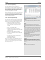
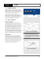
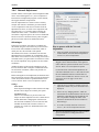
1.1 Waypoint Products Group
Software Overview
NovAtel's Waypoint Products Group offers GNSS postprocessing software packages including GrafNav (a static/
kinematic baseline processor) and GrafNet (a static
baseline processor/network adjustment package). Both of
these products have a Windows based Graphical User
Interface (GUI) and use the same precise GNSS
processing engine. This processing engine has undergone
years of development effort and has been optimized to
give the highest precision with the least amount of
operator intervention.
This chapter contains a description of the hardware
requirements, installation instructions and lists the CD
contents. This chapter also provides an overview of the
product packages (see Table 1, Product Capabilities on
page 18).
How to install Waypoint software
1.
1.2 Installation
Waypoint software supports USB licensing as well as
software-based licensing. Installation instructions for both
are provided in the shaded box.
1.2.1
What You Need To Start
All installation files are provided on both an FTP
site and a password protected website. Contact
[email protected] with your USB license
number or your FlexNet activation ID for login
instructions if these are required.
Sentinel USB Key or FlexNet Activation ID
A software license (USB or software-based) is required to
convert raw GNSS data1, use the Download Service
Utility and to process.
In either case, the license must be detected locally on the
computer running the software. Remote desktop
connections are only supported in a GrafNav term license.
If interested in GrafNav term licensing, contact your local
NovAtel sales representative or [email protected] for
more information.
2.
Launch the setup and follow the on-screen
instructions.
3.
If you are upgrading from a previous major
version, such as 8.50, you will need to upgrade
your USB hardlock key or FlexNet license.
For USB hardlock upgrade instructions, see
Section 1.2.3, How to Upgrade Your Hardlock
Key on page 12. For FlexNet upgrade
instructions, see Section 1.2.4, How to Activate
Your FlexNet License on page 14 or Section 1.2.5,
How to Manually Activate/Return Your FlexNet
License on page 14.
4.
To copy customized settings from a previously
installed major version (i.e. 8.50), access the
Copy User Files program within version 8.60.
This can be accessed from Start | Programs |
Waypoint GPS 8.60 | Utilities | Copy User Files.
Installation file
You will receive an installation CD as part of your
purchase. If you upgrade from a previous version, you will
be provided with a link to Waypoint’s FTP site where you
can download the new setup file.
If you are restricted from connecting to FTP sites for
security reasons, the 8.60 setup files are also available on a
password protected website.
See Prerequisites on page 9 for the hardware requirements.
1. No license is required to convert NovAtel data to Waypoint
format.
GrafNav / GrafNet 8.60 User Guide Rev 3
If you have a previous version of Waypoint
software installed, we do not recommend
uninstalling it prior to installing a new version.
This is because any user created content, such as
favourites, processing profiles, customized grids
or conversions etc., can be copied over to the new
version. This is only possible if the new version is
installed prior to uninstalling the old version.
Separate installation files are provided for the
USB and software-based versions of software. It
is important to download the appropriate
installation file for the type of licensing
purchased.
11
Chapter 1
Introduction and Installation
1.2.2
CD Contents and Installation
GrafNav / GrafNet is distributed on a CD. The latest
version is also kept on our 8.60 FTP site and a password
protected web page. Contact [email protected] to
obtain login information if required.
There are a number of folders on the CD and the FTP site
that contain additional programs and data. These include
the following:
Data
This directory contains sample GNSS data for GrafNav
and GrafNet. Browse through the subdirectories to see
what data is available. To process, copy the contents of
directories to the hard disk.
Geoids
This directory contains geoid files for the U.S. (Geoid03,
Geoid09, Geoid12 and Geoid12A), Mexico97, Australia
(AusGeoid93 and AusGeoid98) and the world (EGM96,
EGM2008). It also contains geoid files for other regions.
These files allow mean-sea-level (orthometric) heights to
be computed using GrafNav and GrafNet. Files are in the
WPG (Waypoint Geoid) format. Contact
[email protected] for more information about geoid
availability for other regions.
All Waypoint geoids are also available for download
directly on our website: www.novatel.com/support/
waypoint-support/waypoint-geoids/
Doc
Contains this manual in Adobe Acrobat PDF format.
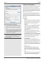
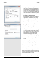
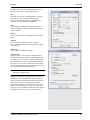
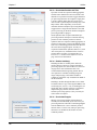
1.2.3
How to Upgrade Your Hardlock
Key
This section applies to customers who are:
• using the hardlock-protected version of Waypoint's
software
• upgrading to a newer version of the software
(i.e. Version 8.50 to 8.60)
• upgrading to a new software package
(i.e. GrafNav to Inertial Explorer)
• upgrading from a demo code to a full license
• applying a demo code to their key
(i.e. time-limited trials)
12
GrafNav / GrafNet 8.60 User Guide Rev 3
Introduction and Installation
1.
Chapter 1
Plug the USB Hardlock Key into an available port
on your computer.
 The hardlock-protected version of the software only
supports Sentinel USB keys. If you have a parallel
port key, contact your NovAtel sales representative to
have it exchanged.
2.
Install the software that you intend to use.
The Sentinel drivers will be installed if it is your
first time using Waypoint software or if your
current drivers are out-of-date.
3.
From the Start menu, navigate to the Utilities folder
within the software’s program group and open the
Hardlock Upgrade Utility.
 Check that the version number in the title bar is at
least 8.30. Older versions of the utility will not work
if you are upgrading to Version 8.30 or newer.
4.
Click the Read Key button to view the information
that is currently written to your hardlock key. This
helps to ensure that the key has been detected and is
communicating properly.
5.
Copy the 16-character code that was provided to
you by Customer Support.
6.
Paste the code into the Hardlock code box and
verify that the information that appears in the
Hardware Key Info area is correct.
If the window does not populate, double-check that
you have entered the code correctly and that there
are no trailing spaces.
7.
When the information appears properly, click the
Upgrade button.
Click the Yes button on the Update Key
confirmation dialog box.
If everything is successful, you will receive the
Update Key Success dialog box.
You are now ready to use the software. You can verify that
the code was properly written by clicking the Read Key
button again.
GrafNav / GrafNet 8.60 User Guide Rev 3
13
Chapter 1
Introduction and Installation
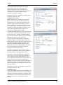
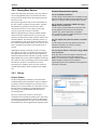
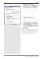
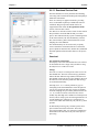
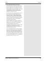
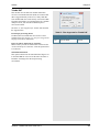
1.2.4
How to Activate Your FlexNet
License
This section applies to customers who wish to activate a
new FlexNet license or upgrade an existing license in
order to use Waypoint software.
 This procedure requires an Internet connection.
If you do not have an Internet connection, skip to
Section 1.2.5, How to Manually Activate/Return Your
FlexNet License on page 14.
1.
Install the Waypoint software that you intend to use.
Contact Customer Support if you need help locating
the setup file on the FTP server.
From the Start menu, navigate to the Utilities folder
within the software’s program group and open the
Local License Manager.
2.
Alternatively, you can navigate to the software's
installation folder on your computer and open the
LLMForm.exe file.
3.
If you are upgrading an existing license, you will
first need to return the original license. Do this by
selecting your existing license under Local Licenses
and then clicking the Return button.
4.
Copy the alpha-numeric Activation ID that was
provided to you by Customer Support and paste it
into the box under the Activate License branch.
5. After the Activation ID has been entered, click the
Activate button.
6.
If the license was successfully activated, you will
see it appear under the Local Licenses branch. Click
on the license to see the relevant information.
If you have activated a term license, then the
expiration date will be displayed here.
If the activation fails, contact Customer Support
([email protected]).
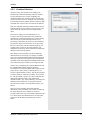
1.2.5
How to Manually Activate/Return
Your FlexNet License
The section describes how to activate and/or return a
FlexNet license when no Internet connection is available
or you are unable to access NovAtel's license server.
 If you are upgrading an existing license, your original
license will need to be returned prior to activating the
upgrade (see the instructions in Manual Return
Process on page 16 first).
14
GrafNav / GrafNet 8.60 User Guide Rev 3
Introduction and Installation
Chapter 1
Manual Activation Process
1.
Open a console window and navigate to the
software's installation folder
(e.g. C:\NovAtel\InertialExplorer860).
2. Enter the following command to generate a Manual
Activation Request.
llmform -am ActivationID OutputFile
Where:
ActivationID is the alpha-numeric Activation ID
provided to you by Customer Support
OutputFile is the output XML file that will contain
the request
Sample usage:
llmform -am 1a2b-3cf4-5e6f-1a2b3c4d-5e6 c:\temp\activate_req.xml
3.
Send the output file that was generated in the
previous step to NovAtel Customer Support
([email protected]). Note that this file is
simply an ASCII XML file.
4.
Customer Support will send back a new file
containing the response. To process this response,
navigate back to the installation directory and enter
the following command:
llmform -p InputFile
Where:
InputFile is the file that was sent back to you by
Customer Support
Sample usage:
llmform -p c:\temp\activation_
response.xml
5.
If this is the first manual activation on a machine,
the license will not be activated on the machine at
this point, because the first response file is simply a
configuration response. You will need to repeat
steps 1 - 4 in order to re-submit the request and
complete the activation.
6.
The license should now be activated. To check,
enter the following command:
llmform -v
Or open the Local License Manager and look under
the Local Licenses branch.
GrafNav / GrafNet 8.60 User Guide Rev 3
15
Chapter 1
Introduction and Installation
Manual Return Process
1.
2.
Open a console window and navigate to the
software's installation folder (e.g.
C:\NovAtel\InertialExplorer850).
Enter the following command to generate a Manual
Return Request:
llmform -rm ActivationID OutputFile
Where:
ActivationID is the alpha-numeric Activation ID
provided to you by Customer Support
OutputFile is the output XML file that will contain
the request
Sample usage:
llmform -rm 1a2b-3cf4-5e6f-1a2b3c4d-5e6 c:\temp\return_req.xml
3.
Send the output file that was generated in the
previous step to NovAtel Customer Support
([email protected]). Note that this file is
simply an ASCII XML file.
4.
Customer Support will send back a new file
containing the response. To process this response,
navigate back to the installation directory and enter
the following command:
llmform -p InputFile
Where:
InputFile is the file that was sent back to you by
Customer Support
Sample usage:
llmform -p
c:\temp\return_response.xml
5.
16
The license should now be returned. To check, open
the Local License Manager and look under the
Local Licenses branch to ensure that the license is
no longer listed.
GrafNav / GrafNet 8.60 User Guide Rev 3
Introduction and Installation
Chapter 1
1.3 Processing Modes and
Solutions
Processing Solutions
The types of solutions are described in the shaded box.
The following are the types of processing modes:
AdVance RTK® is NovAtel's industry leading RTK
engine which provides rapid centimetre level
positioning. ARTK is used in Waypoint products to
resolve integer carrier phase ambiguities.
Static
Static processing involves the determination of a single
coordinate for an entire static session. There are two types
of static solutions supported by GrafNav: float and fixed
solutions. They are discussed in the shaded box.
Kinematic
When processing kinematic data, it is of interest to
optimize the entire trajectory. This is in contrast to static
processing, which solves one coordinate for the entire
session.
In order to quickly achieve cm-level accuracy in kinematic
processing environments, ARTK is used to resolve integer
carrier phase ambiguities. This is discussed in the shaded
box.
ARTK solution
With short baseline lengths (several kilometres), open
sky conditions and dual frequency data, ARTK often
requires only several seconds of data. Although ARTK
needs at least 5 satellites to resolve, in practice it is most
robust when 7 or more satellites are available. ARTK
may resolve at baseline lengths as long as 70 km,
however it is most reliable at distances of 30 km and less
provided dual frequency data.
Fixed static solution
The fixed static solution uses ARTK with static
constraints to resolve integer carrier phase ambiguities.
When ARTK returns a successful fix it is automatically
re-engaged. A history of ARTK solutions over the static
session is kept and GrafNet allows you to choose which
is accepted as the final solution based on estimated error,
lowest RMS, highest reliability, or an average of all
fixes.
Float solution
Float solutions, unlike fixed static and ARTK solutions,
do not resolve carrier phase ambiguities as integers. As
such, they are associated with lower accuracy
applications than fixed solutions. Provided good data,
float solutions improve with time and can still achieve
sub decimetre accuracy, depending on other factors such
as baseline length, number of satellites and geometry,
raw measurement data quality, etc.
GrafNav / GrafNet 8.60 User Guide Rev 3
17
Chapter 1
Introduction and Installation
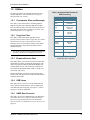
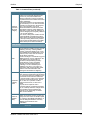
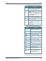
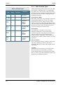
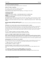
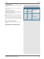
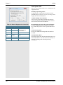
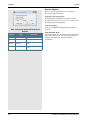
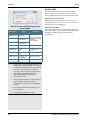
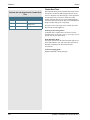
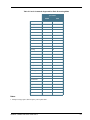
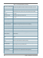
1.4 Overview of the Products
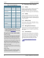
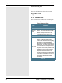
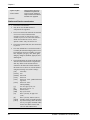
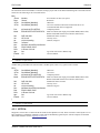
Table 1: Product Capabilities
Capabilities
Float Static
GrafNav Static
GrafNav/GrafNet



Float Kinematic
Fixed Integer Static
(Fixed Solution)



Fixed Integer Kinematic
Dual Frequency


GPS, GLONASS and
BeiDou Support



Multi-Base Processing
PPP
(Static only)

Moving Baseline

Azimuth Determination

Remote Desktop
Compatibility
a
Batch Processingab
(Static only)

IMU Processingc
a. Available only if a term license is purchased.
b. For more information about batch processing, see
Appendix A, WPGCMD on page 167.
c. Refer to the Inertial Explorer User Manual available
on our website at www.novatel.com.
Moving Baseline Features within GrafNav
Relative Processing
All of the same advanced GrafNav processing features
including ARTK, a robust Kalman filter, and forward/
reverse processing are also supported in moving base
processing. The only restriction is that only one base
station can be used when processing the relative vector.
For applications where both antennas are mounted on the
same vehicle, the surveyed distance between the
antennas can be entered to assist ambiguity resolution.
Heading can also be computed for these applications.
1.4.1
GrafNav
GrafNav is a kinematic and static GNSS post-processing
package. Included with GrafNav is a Precise Point
Positioning (PPP) module, support for multi-base
applications, and support for moving base applications.
See Chapter 2, GrafNav on page 21 for more information.
1.4.2
GrafNet
GrafNet is a batch static baseline processor and network
adjustment package. It is often used to check or establish
base station coordinates for later use within GrafNav or to
survey static networks. See Chapter 3, GrafNet on page 99
for more information.
1.4.3
GrafNav Static
GrafNav Static includes GrafNav and GrafNet, however
only static data can be processed. See Chapter 2, GrafNav
on page 21 for more information.
1.4.4
Moving Baseline Features
GrafNav features a moving baseline module that processes
GNSS data between two moving antennas. Heading can
also be computed if the two antennas are mounted on the
same vehicle
1.4.5
Inertial Explorer
Inertial Explorer shares a similar interface with GrafNav
and provides both GNSS and INS processing capabilities.
Inertial Explorer is powerful and feature rich, including
support for both loosely and tightly coupled processing,
multi-pass processing, a backsmoother, automatic
processing profile detection and many other features.
See www.novatel.com/products/software/inertialexplorer/ for more information.
Relative Vector Output
After processing, the included Export Wizard profiles
are available to output the relative vector in local level or
ECEF format.
Relative Velocity
In addition to relative position information, GrafNav
uses Doppler measurements to compute instantaneous
relative velocity between two moving antennas.
18
GrafNav / GrafNet 8.60 User Guide Rev 3
Introduction and Installation
Chapter 1
1.5 Utilities
The following utilities are installed automatically with
GrafNav and can be accessed from Start | Programs |
Waypoint GPS 8.60 | Utilities.
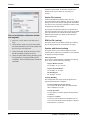
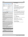
1.5.1
Concatenate, Slice and Resample
This utility is most often used for combining multiple
GPB files together and resampling GPB files to higher
intervals. There are many other uses of this utility however
and a full description can be found in Concatenate, Slice
and Resample Overview on page 142.
1.5.2
Copy User Files
This utility is intended for those upgrading from a
previous version (such as 8.50). It copies any user created
content from a previous version to the new version.
Examples of user created content include custom datum
and grid definitions, Export Wizard profiles and user
defined favourites.
 It is for this reason we do not recommend uninstalling
previous versions prior to installing version 8.60.
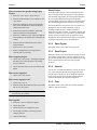
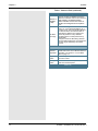
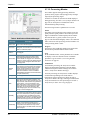
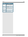
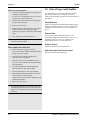
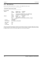
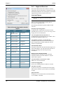
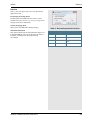
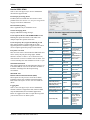
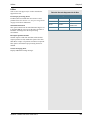
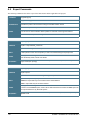
1.5.3
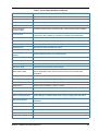
Download Service Data
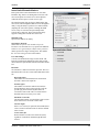
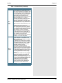
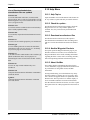
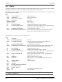
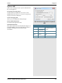
Table 2: Supported Data Formats for
Post-Processing
Make
Model
NovAtel
All Models
Javad
All Models
Leica
System 500
System 1200
GX1230
NavCom
SF-20x0
SF-30x0
Sapphire
RTCM
3.0
Septentrio
SBF
Ashtech/
Thales/
Magellan
Real Time
B-file
Trimble
DATa
U-Blox
Antaris
RINEX
2.x
3.x
a. Decoding of only GPS data from
Trimble DAT files is supported.
This utility allows you to search for freely accessible base
station data provided by government organizations. The
utility fully supports GPS, GLONASS and BeiDou and
will download, convert, and if necessary resample and
concatenate the downloaded data so that it is ready to be
used within your project.
The download utility can also be used to obtain precise
satellite clock and ephemeris data, almanacs and alternate
broadcast ephemerides.
1.5.4
GPB Viewer
This utility allows you to view converted GNSS data as
well as perform certain functions, such as changing the
static/kinematic processing flag. See Chapter 5, Utilities
on page 137 for more information.
1.5.5
GNSS Data Converter
This utility converts raw GNSS data files into Waypoint’s
own format. See Table 2, Supported Data Formats for
Post-Processing for supported receivers and formats.
Also, see Section 5.4, GNSS Data Converter Overview on
page 143.
GrafNav / GrafNet 8.60 User Guide Rev 3
19
Chapter 1
Introduction and Installation
IMU Data Converter also appears under the utilities group
when you install. Also, depending on which version (USB
or FlexNet) you installed you will either see the Hardlock
Upgrade utility or a Local License Manager.
20
GrafNav / GrafNet 8.60 User Guide Rev 3
Chapter 2
GrafNav
2.1 GrafNav and GrafNav Static
Overview
GrafNav
GrafNav is a full-featured kinematic and static GNSS
post-processing package that uses a proprietary GPS,
GLONASS and BeiDou processing engine. It supports
single and multi-baseline (MB) processing, moving
baseline processing, Precise Point Positioning, and
directly supports many different receiver formats. For any
receiver formats not currently supported, RINEX files can
be imported. See Table 2, Supported Data Formats for
Post-Processing on page 19 for more information.
This chapter describes how to get started with GrafNav
and goes through each menu of its interface. Step-by-step
instructions for first-time users are also included.
GrafNav Static
This chapter also describes the features of GrafNav Static.
GrafNav Static provides the same processing features as
GrafNav, but only for static baselines.
See Table 1, Product Capabilities on page 18 for a
capability comparison between GrafNav and GrafNav
Static.
GrafNav / GrafNet 8.60 User Guide Rev 3
21
Chapter 2
GrafNav
2.2 Start a Project with GrafNav
New users will find it easiest to create a new project with
the New Project Wizard. The Wizard takes you through all
the steps of creating a GrafNav project, including data
conversion and downloading base station data (if needed).
The only requirement for using the Wizard is that you
have a raw GNSS data file downloaded to your computer.
Access the Wizard through File | New Project | Project
Wizard.
After you have become familiar with the GrafNav
interface, you may prefer to create new projects using the
Empty Project method. When creating an empty project,
you need to first convert your data using the Raw GNSS
conversion utility and download any base station data
using the Download Service Utility. See Section 5.4,
GNSS Data Converter Overview on page 143 for a
description of the Convert Utility, and Section 2.8.11,
Download Service Data on page 92 for instructions on the
Download Utility.
Before you start a project in GrafNav, you need to verify
installation, convert data and download any required data.
Install Software
Verify that the installation was successful by ensuring that
you have a Waypoint program group on your computer. If
this program group is not there, see Chapter 1,
Introduction and Installation on page 11 for installation
instructions.
Convert Data
Raw GNSS data files must be converted into Waypoint’s
GPB format. If creating a project through the New Project
Wizard, there is no need to convert your data first. If
creating an empty project, the Raw GNSS Converter must
be used before creating a project. See Section 5.4, GNSS
Data Converter Overview on page 143 for a complete
description of the Convert utility.
Download Service Data
If no data was logged from a reference station, you have
the option of downloading free GNSS data from the
Internet.
A reference station can also be added directly from a list.
See Section 2.8.11, Download Service Data on page 92 for
these instructions as well as a complete description of the
Download utility.
22
GrafNav / GrafNet 8.60 User Guide Rev 3
GrafNav
Chapter 2
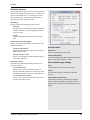
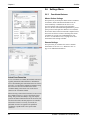
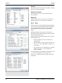
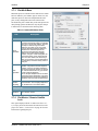
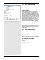
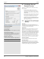
2.3 File Menu
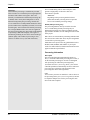
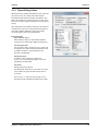
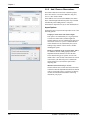
2.3.1
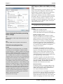
New Project
To process a survey for the first time, start a new project.
When you start a new project, choose between Project
Wizard and Empty Project.
The Project Wizard is recommended for new users as it
will guide you through all the steps of getting started,
including data conversion and downloading base station
data (if needed). After you are more familiar with
GrafNav's tools and workflow, you may prefer to use the
Empty Project option.
This section discusses these options and gives step-by-step
instructions once you have decided on the method for
starting your project.
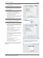
Project Wizard
Project Wizard Steps
1.
Create and name the project.
2. Add rover data to the project.
 The rover data can be in Waypoint’s GPB format, or
in the receiver’s raw format, in which case the
Wizard converts it to GPB for you.
3. Add base station data to the project.
 You can add your own local base station data (in
raw or GPB format) or you can have the Wizard
download free service data from the Internet.
If you plan to process with PPP, you can skip adding
base station data and download the precise satellite
clock and orbit files from the Internet
The Project Wizard offers you a guided step-by-step way
of creating a project. The Project Wizard steps are listed in
the shaded box
GrafNav / GrafNet 8.60 User Guide Rev 3
23
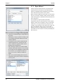
Chapter 2
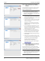
How to create a new project using Empty
Project
GrafNav
Empty Project
Creating an empty project is not recommended for new
users as all steps involved with project creation must be
done manually. Specifically, the remote GNSS data must
be converted to GPB format using the GNSS Data
Converter utility and any base station service data must be
downloaded through the Download Service Data Utility.
1.
Select File | New Project | Empty Project.
2.
Enter the name and where you would like to save
your project.
3.
Select File | Add Master File(s) to load master
files. Select the GPB files collected at the base
station(s) and click Open.
4.
Enter the base station coordinates, datum and
antenna information when prompted.
5.
Select File | Add Remote File. Select the GPB file
corresponding to the data that was collected at the
remote.
The Project Wizard is best for new users as it guides you
through each step involved with starting a project.
Creating an empty project is usually preferred by
advanced users. This is because, for someone familiar with
GrafNav's workflow, it may be possible to get started more
quickly creating an empty project as opposed to going
through each step of the Wizard. The steps involved with
creating an empty project are in the shaded box.
6.
Enter the antenna information for the remote
when prompted.
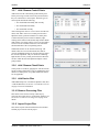
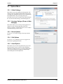
2.3.2
7.
Select Process | Process GNSS.
This option allows you to open existing projects.
8.
Ensure an appropriate processing profile is
selected prior to processing.
2.3.3
How to open a project
1.
Choose File | Open Project. A dialog box appears
that asks you to select the name of an existing
project (CFG file).
2.
Choose the name of the project and click the OK
button.
How to save a project
1.
Choose File | Save Project.
Open Project
Save Project
When this option is selected, all project settings are saved
to a GrafNav configuration (.cfg) file. GrafNav saves the
project automatically when processing and thus accessing
the save option from the file menu is not typically
necessary.
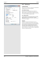
2.3.4
Save As
Use the Save As command under the File menu to create a
new project that has identical processing options as the
current project. This allows you to change the options in
the new project and process the data without losing the
solution computed by the original configuration.
How to save a project “as”
1.
Choose File | Save As.
2.3.5
Print
2.
Enter the name, file format and where you would
like to save your project.
This option allows you to print various items including
windows, plots and text files.
 Entering the name of a project that already exists
overwrites the file contents.
How to print
24
1.
Select File | Print. A dialog box appears.
2.
Choose the printer.
3.
Choose the item you would like to print.
4.
Set the page orientation, color and any other
settings you need.
5.
Click the OK button.
GrafNav / GrafNet 8.60 User Guide Rev 3
GrafNav
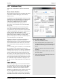
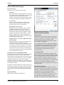
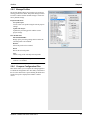
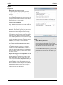
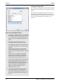
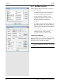
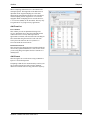
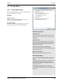
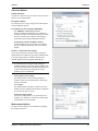
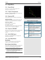
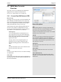
2.3.6
Chapter 2
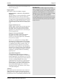
Add Master File(s)
Steps for how to add a master station are in the shaded
box.
Master Station Position
When loading a master station, the coordinates that appear
in the master coordinate dialog may come from two
different sources.
If loading data converted from RINEX, as is the case when
obtaining base station data through the Download Service
Data Utility, the coordinates that appear initially are
scanned from the RINEX header. The coordinates
provided in the RINEX header may be precise or
approximate, this will depend on the individual RINEX
data provider.
If loading base station data converted from any other
source, the coordinates that appear initially are likely
averaged from the unprocessed position records decoded
in the raw GNSS data file. The accuracy of this position is
typically no better than approximately 2 metres
horizontally and 5 metres vertically. If you select the OK
button using averaged coordinates, a warning dialog
appears to ensure you are aware the coordinates may not
be accurate enough for your application.
Regardless of the source of your base station data, it is
important that accurate coordinates are loaded. In
differential processing, a vector is solved between the base
station antenna and the remote antenna. Any error in the
base station position is directly transmitted to the remote
position.
To assist in loading precise coordinates, it is recommended
that coordinates be selected from the favourites list
through the Select from Favourites option. Coordinates for
select base station networks, such as CORS and IGN, are
regularly maintained and accessible through Favourites.
The Compute from PPP option can be used to easily check
or survey base station data using GrafNav's Precise Point
Processor. When using this option, the difference between
the loaded and computed coordinates is displayed. Note
that PPP accuracy is largely dependent on the length of the
survey.
How to add a master file
1.
Select File | Add Master File(s).
2.
Select the base station file(s) from the list of
available GPB files. Up to eight base stations can
be added to a GrafNav project. Click the Open
button.
3.
Enter the coordinates of each base station when
prompted.
4.
Verify that the coordinates match your selected
processing datum.
5.
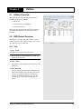
Enter the antenna model and height information
and click the OK button.
Datum Selection
In differential processing, a vector is solved between the
base station and the remote. Your project datum is thus not
controlled by what you select as your processing datum,
but rather the actual base station coordinates entered.
Regardless, it is important to ensure you have correctly set
the processing datum after entering the base station
coordinates. This is partly because the processing datum is
documented in the header of all export files generated by
GrafNav / GrafNet 8.60 User Guide Rev 3
25
Chapter 2
GrafNav
the Export Wizard. If it is incorrectly set, your results
could be interpreted by another person as being in the
incorrect datum.
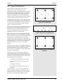
Antenna Height
The antenna height entered in this box applies primarily to
kinematic trajectories and static sessions. If exporting
camera marks/features, you are provided the opportunity
to apply an offset during export. As such, if you are
interested primarily in exporting camera events, we
recommend entering an antenna height of zero as
measured to the Antenna Reference Point (ARP).
Antenna Models
The purpose of an antenna model is to:
• Correct for the vertical offset between where
GNSS observations are observed (the electronic
phase center) and the bottom of the antenna
(Antenna Reference Point, or ARP).
• Correct for any difference between the L1 and L2
electronic phase centers, which can be a factor in
the success or failure of ambiguity resolution.
• Apply small elevation based corrections (mm
level)
GrafNav 8.60 supports absolute antenna models as
provided by the NGS. If the antenna model is not known at
your remote, it is recommended that the Generic profile be
applied, which does not apply any corrections. In that
case, the processed position is referenced to the antenna
L1 phase center. However, the correct antenna model
should be selected for best results.
When selecting an antenna model, the Applied height
reflects the vertical offset between the L1 phase center and
the ARP (which is the bottom of the antenna). This value
comes directly from the antenna model and reduces the
processed position from the phase center to the bottom of
the antenna. This value should match any diagram that
appears directly on your antenna, presuming it is an
absolute antenna calibration. Antenna heights can be
measured to the antenna reference point, phase center, or
computed from a slant measurement.
When loading a base station converted from RINEX, the
antenna name and radome (if provided) are scanned from
the RINEX header and used to automatically load the
appropriate antenna profile. It is good practice to ensure
the correct antenna model is loaded prior to processing.
26
GrafNav / GrafNet 8.60 User Guide Rev 3
GrafNav
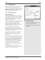
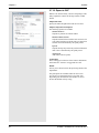
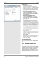
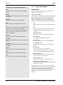
2.3.7
Chapter 2
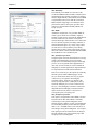
Add Remote File
The remote file contains the raw GNSS measurements that
are processed together with data from known base
station(s). The remote file must be converted to GPB prior
to loading. When adding a remote GPB file, you are
prompted to enter the antenna information. See Antenna
Models on page 26 for more information.
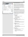
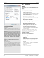
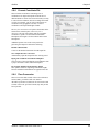
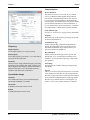
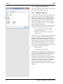
2.3.8
Add Precise Files
Broadcast Ephemeris
The ephemeris file contains Keplerian orbital parameters
used to compute satellite positions. Presently, the line of
sight component of satellite positions can be computed
within an accuracy of approximately 2 metres (RMS)
using the broadcast ephemeris.
Orbital error is largely removed in differential processing,
as the line of sight component of orbital error is heavily
correlated at short and medium baseline lengths.
Therefore, the accuracy of the broadcast obits is
completely sufficient for most projects. A discussion on
precise orbits is found in the next section.
Generally, the GNSS receiver includes broadcast
ephemeris data with its raw data files. The decoder
converts these files into EPP format. Receivers typically
output ephemerides at startup, as satellites rise into view,
or approximately every two hours.
How to add a remote file
1.
Select File | Add Remote File.
From the list of available GPB files, choose the
file collected at the remote station.
2.
When prompted, enter the remote station antenna
information.
Prior to processing, GrafNav combines all ephemeris
information collected at the base station(s) and remote.
This minimizes the chance of missing broadcast
ephemerides.
In version 8.50 and earlier, if a GPS broadcast ephemeris
was missing the satellite could not be used regardless of
whether or not a precise ephemeris file had been added to
the project. Version 8.60 is less dependent on the presence
of GPS and BeiDou broadcast ephemerides and any
missing broadcast values can be fixed by adding a precise
ephemeris to the project. The same is not true for
GLONASS, broadcast ephemerides are required
regardless of whether a precise ephemeris has been added
to the project.
The Download Service Data utility can be used to
download a global broadcast ephemeris file in EPP format
as well as to download precise ephemerides.
GrafNav / GrafNet 8.60 User Guide Rev 3
27
Chapter 2
GrafNav
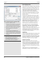
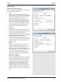
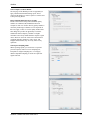
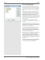
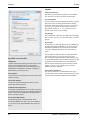
Precise Ephemerides
Precise ephemerides are computed from data collected by
ground reference stations around the world. These files are
produced by various agencies, including CODE (Center
for Orbit Determination), the IGS, and many others. The
different precise ephemeris products vary in their latency,
with presently supported products ranging from
approximately 6 hours to 2 weeks. The difference in
accuracy between rapid and final products is very small,
generally within the noise of either differential or PPP
kinematic solutions.
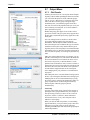
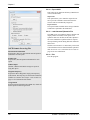
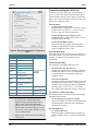
How to download precise ephemeris files
1.
Select File | Add Precise Files.
The project start and end date are automatically
scanned from the GNSS data loaded into the
project. This should not need to be set manually.
2.
Select Browse in order to choose any precise
orbits (.sp3) that have previously been
downloaded.
If no files have been downloaded, select
Download and the precise orbit (.sp3) and clock
(.clk) data will automatically be downloaded and
added to your project. This requires an internet
connection.
 If your project includes GLONASS or BeiDou data
make the appropriate selection under the
Constellation pull down menu prior to
downloading. The default search location for
precise products contains only GPS data.
Presently, precise ephemerides reduce the line of sight
component of satellite position error to approximately 2
cm RMS (as compared with approximately 2 m RMS for
broadcast orbits). As orbital error is largely cancelled in
differential processing, adding precise ephemerides to a
differential project will only produce observable
differences where the baseline length is very large (150200 km). For this reason, adding precise orbits to a
differential project is generally considered optional.
Precise ephemerides can be downloaded through the
Download Service Data utility or directly through the
GrafNav interface. The latter method is described in the
shaded box. Adding a precise ephemeris file will
compensate for any missing broadcast ephemeris data for
GPS and BeiDou satellites. A broadcast ephemeris for
each GLONASS satellite observed is required regardless
of the presence of a precise ephemeris.
IONEX Files
IONEX (Ionosphere Map Exchange) files contain a model
of the TEC (Total Electron Content) of the ionosphere.
These files can be applied to assist long distance L1 only
processing. As such, these corrections are not of interest to
the majority of GrafNav users. These files are ignored if
dual frequency ionospheric processing is engaged.
Satellite Clock Files
Presently, using the data available in the broadcast
ephemeris, satellite clock errors can be predicted within an
accuracy of approximately 2 m RMS. Satellite clock error
is completely removed in differential processing, as this
error is exactly the same at the base and the rover. Thus
adding precise clock files to a differential project will have
no effect.
Satellite clock files can be downloaded through the
Download Service Utility or from File | Add Precise Files.
28
GrafNav / GrafNet 8.60 User Guide Rev 3
GrafNav
2.3.9
Chapter 2
Load
GNSS Solution
After processing, forward and reverse solutions are
automatically combined if available. Thus the trajectory
output to the map window, and all generated plots, are
usually relative to a combined forward/reverse solution.
The title bar of the map window and plots clearly indicate
which solution is loaded.
If the processing results from a particular direction
(forward or reverse) are of interest, individual solutions
can be loaded using this feature.
PPP Solution
GrafNav's differential and PPP trajectory files have, by
design, different file extensions. This allows both
differential and PPP trajectories to be processed within the
same project without overwriting each other. If both types
of solutions have been processed, you can control which
type of solution is loaded through the GNSS Solution and
PPP Solution options.
Any Solution
This option allows any GrafNav readable trajectory to be
loaded into a project. The only requirement is that the
trajectory cover the same time range as the data within
your existing project. An example of when this feature
may be used is when loading a real time trajectory
produced from the GNSS decoder.
Single Point Solution (from .gpb file)
This option ensures the trajectory displayed to the map
window reflects the unprocessed positions in the remote
GNSS data. This trajectory typically represents the real
time solution as computed on board the receiver during
data collection.
GrafNav / GrafNet 8.60 User Guide Rev 3
29
Chapter 2
GrafNav
Loading Camera Event Marks
Use this feature to load external time-tagged events from
an ASCII file. When you load these events, they must be
referenced to GPS time and not UTC (coordinated
universal) time. The source of the events can come from
an aerial camera, sounding equipment or other real-time
devices. The GPS receiver must support a mark or pulse
input for this feature to work.
Most events are automatically stored in the station file
(.sta) during the conversion to GPB format and appear
when the remote is added to the project. For user events,
and a few receivers such as Ashtech or B-file, this feature
must be used.
File Format
STA File
Many new converters save the camera event marks
directly to the station file. The marks load when you
add the GPB file to the project. If they do not load,
then use the File | Load | Station File feature.
How to load camera event marks
1.
Under File, select Load | Camera Event Marks.
2.
Choose the file format that matches your input
file.
3.
Under File Name, use the Browse button to select
the file of interest. The file name depends on the
receiver format and is explained in Section 2.3.6,
Add Master File(s) on page 25.
 If the files formats you use are User1- User6, use
Time Settings to select the time formats. UTC time
cannot be loaded and the correction has to be
applied externally.
MRK File
Leica SR receivers save event marks into a EVT file,
which is converted into a MRK file by the Leica
decoder. The MRK file can be loaded using this
option. Numbering is performed by the converters.
Ashtech Download
Ashtech receivers with internal memory usually
output a PHOTO.DAT file after the receiver data has
been downloaded using HOSE or another
corresponding utility. Newer variants might be under
the format M????.###. Either file can be loaded using
this option. The GMT date of the first event mark
must be entered if it is not detected. Events are
automatically numbered starting at 1.
Leica GeoSystems
EV0 and TDU files are produced by the Leica
software and can be imported using this option. This
file might contain time in the local time zone. If not,
enter the time zone offset as zero. The time zone
correction and the GMT date of the first mark must be
entered. Events are automatically numbered starting
at 1.
LH-Systems Ascot
LH Systems ASCOT (RC-30) has a format very
similar to EV0 except that it contains the relative
angles of the camera mount, which can be used to
apply a 3-D offset for the antenna/camera difference.
User#
These formats allow you to import the time and name
of each event mark. Optional variables include line
number (description) and altitude information.
30
GrafNav / GrafNet 8.60 User Guide Rev 3
GrafNav
Chapter 2
File Name
The file name depends on the receiver format. Examples
include the following:
• NovAtel is MRK
• Ashtech is PHOTO.DAT
• Trimble is SUM
• Leica is EVO
Time settings
User time type:
Seconds of the week – GPS time ranging from 0 to
604800.
Local H:M:S – Local hours, minutes and seconds
(HH:MM:SS.SSSS).
GMT H:M:S – GMT hours, minutes and seconds
(HH:MM:SS.SSSS).
Local time correction:
This is necessary for both Leica and User# formats
using Local H:M:S. This is the offset, in hours, from
GMT. For the Eastern Standard Time zone, this
number is 5. For the Pacific Standard Time zone, this
number is 8. During daylight savings time, these
numbers are reduced by one. An incorrect entry
causes the camera marks to be displayed incorrectly
or not be displayed at all.
GMT date of first record:
This is necessary for Leica, Ashtech and User#
formats implementing H:M:S time-tagging. Enter the
date of the first exposure record in month/day/year
format. It is not the date in local time, which may
differ towards the end of the day. An invalid date
results in the marks not being displayed.
Attitude Format
For User5 and User6 formats that include attitude
information, a definition of how the angles are defined is
required. Currently, the following attitude formats are
supported:
Photogrammetric (w-p-k):
These angles are defined as omega primary, phi
secondary and kappa tertiary (ground-to-air).
Camera (roll, pitch, drift):
These angles are the relative ones between the frame
of the camera and that of the aircraft.
If the raw GPS receiver data logs position records, there
are small circular event marks on the trajectory map in
bright blue. These also appear if the data has been
processed. If no event marks are present after processing,
then it is likely that the time tags are wrong or no event
GrafNav / GrafNet 8.60 User Guide Rev 3
31
Chapter 2
GrafNav
marks have been loaded. To determine what has been
loaded, use the Feature Editor by selecting View |
Features.
Station File (.sta/nst)
GrafNav automatically loads the station file (.sta)
associated with the remote GPB file. This file is produced
during conversion and contains, among other information,
any camera events. If properly loaded, these camera events
are displayed to the map window.
How to load Stations with known latitude
and longitude
1.
2.
Select File | Load | Stations with Known Lat/
Long.
Choose the file, under File Name, that contains
the station information in one of the formats from
the Lat/Long Format option list.
3.
Choose the format, under the Lat/Long Format,
that the coordinates from the file are in.
4.
Choose an option under Id String Handling to tell
the program how to separate the ID from the
coordinates. The first column usually contains the
station IDs.
The program automatically loads the STA station file as
long as the filename is the same as that of the remote GPB
file. If the station file has a different filename than the
GPB file, then load the file separately. Most decoders
produce station files.
RTK Dat File (.sta/nst)
This option loads converted RTK solution files and then
uses the Export Wizard to re-format them for output.
Stations with Known Lat/Long
This option allows you to load and display a file that
contains stations with known coordinates. The coordinates
are displayed with pink triangles.
Lat/Long Format
This is a list of formats that the coordinates from the file
are in. These formats include the following:
Degrees Minutes Seconds
For example: 51° 03’ 28.3214”
Degrees Decimal Minutes
For example: 51° 03.4720’
Decimal Degrees
For example: 51.0579°
Id String Handling
The settings under this option tell the program how to
separate the ID from the coordinates.
Use first continuous word (no spaces)
To be used if the station names are separated from
their coordinates by a space.
Comma separation
Use this option if commas separate the IDs from the
coordinates.
Use first ‘n’ columns
If you know which column the coordinates start in,
you can enter the number for the program to begin at.
Each character is a column.
32
GrafNav / GrafNet 8.60 User Guide Rev 3
GrafNav
Chapter 2
Leica IDEX File (.idx)
Time-tagged points created with Leica 5 data collectors
can be given a name, position and antenna height.
However, firmware versions 3.0 and greater do not store
the station names within the TTP file. These names are
stored within the database structure (control.db) and
cannot be accessed directly by the software. The point
information contained within the database has to be
converted to ASCII, which is done by creating an IDEX
file using Leica's Ski software.
Once an IDEX file has been created, it can be loaded into
GrafNav. You should see a message indicating how many
IDEX points were matched to TTP points. After
processing at least one direction, the TTP points should be
visible and numbered sequentially. These have been
loaded from the STA file.
Points are matched via their times. Often, there are fewer
matched points than the original number of TTP points
due to several reasons, including the deletion of points in
the field, and/or the addition of static session marks.
Aschtech OUT File (.out)
This type of file is created by Ashtech’s Seismark
surveying system and can be loaded into a project.
GrafNav / GrafNet 8.60 User Guide Rev 3
33
Chapter 2
GrafNav
2.3.10 Convert
The two conversion utilities that are available are the
following:
Raw GNSS to GPB
You must convert your raw GNSS data files to GPB prior
to creating an empty project. It is not necessary to convert
your raw GNSS data prior to creating a new project if
using the New Project Wizard. See Section 5.4, GNSS
Data Converter Overview on page 143 for more
information regarding this utility.
GPB to RINEX
Convert GPB to RINEX
This utility converts a GPB file into a standard RINEX
file, version 2.0 or 2.11.
Rinex Version
Choose between Version 2.11 and Version 2.0 format.
GLONASS
If present, GLONASS measurement data writes to the
observation file, while the ephemerides write to their
own navigation file. This option can be enabled to create
GPS-only RINEX files.
Files to Convert
Allows you to select the files that are to be converted.
GPS Week
Sets the week number in which the observations were
made. If the Auto-Detect Week button is selected, then
the program determines the week number from the EPP
file. Sometimes, an incorrect week number is output to
the EPP file during the conversion from a raw data
format. In such a case, you must manually enter the
week number via the Set Week button.
GNSS manufacturers typically provide a utility to convert
their native data format to RINEX. It is therefore unusual
to convert from GPB to RINEX, as an intermediate step
would be involved (converting to GPB) when often the
native receiver data can be converted directly to RINEX.
Nonetheless, RINEX 2.11 and 2.0 files can be generated
from GPB files using this utility. See the shaded box for
more information.
2.3.11 GPB Utilities
The GPB Utilities are available for use with GPB files and
includes the following:
Concatenate, Slice and Resample
See Section 5.3, Concatenate, Slice and Resample
Overview on page 142.
View Raw GNSS Data
See Section 5.2, GPB Viewer Overview on page 137.
RINEX Header Information
Several fields are available here for editing. This
information is used only for the purpose of being written
to the header of the RINEX observation file.
 Multiple files can be added for conversion. For each
file added, you are prompted for a station name, an
antenna height, and, if needed, an alternate
ephemeris file.
34
GrafNav / GrafNet 8.60 User Guide Rev 3
GrafNav
Chapter 2
Insert Static/Kinematic Markers
Each epoch in the remote GPB file has its own static/
kinematic flag, which is set during data conversion. The
conversion options for each receiver can be adjusted
within the Global Options of each receiver type.
The static/kinematic flag can also be changed after data
conversion, either through the GPB Viewer or through this
utility. Using this utility is preferred over other methods
(adjusting the conversion options or through the GPB
Viewer) only if it is desired to input multiple static
sessions into a single file. This is because this utility
supports reading start and end times from a file.
GPB File Name
Specifies the GPB file to modify.
Operation to Perform
Select Make all epochs static or Make all epochs
kinematic to set the mode for every epoch in the GPB file.
Select Use user generated file to define static periods to
define specific time ranges as being static. This enables
the User File Settings section on the window.
User File Settings
Converts user-defined time ranges to static mode. The
input file containing the definitions of the static periods
must contain the space-delimited fields listed in the shaded
box.
Space-delimited fields
• StationID
• StartTime
• EndTime
• Description
File name
Click the Browse button to locate the input file. The View/
Edit button allows for the revision and modification of the
file.
Begin time offset
The number of seconds added to all user-defined
StartTime values in the input file.
End time offset
The number of seconds to subtract from all userdefined EndTime values in the input file. Only the
epochs lying between these adjusted times are
converted to static mode. This is to ensure that no
kinematic data is incorrectly set to static.
Minimum session time
The minimum number of seconds that a static session
must contain to be converted to static mode.
Antenna height
If the Create station file option has been enabled, this
value is written to the station file for all user-defined
static sessions.
Create station file
Writes all static sessions to the station file (STA),
regardless of whether an antenna height has been
entered.
GrafNav / GrafNet 8.60 User Guide Rev 3
35
Chapter 2
Files affected by each Remove Processing
Files option
Project(s) to Remove
Allows you to select what project(s) you want to delete
processing files from.
Current project
Only removes the selected files that are associated with
the project that is currently loaded.
All files in
Allows you to select the folder from which you want the
selected files deleted.
Selected projects
Allows you to select a specific project whose associated
files you want to delete.
GrafNav
2.3.12 Remove Processing Files
When processing GNSS data, GrafNav's processor
generates many different file types, both ASCII and
binary. Many of these files are required by the Export
Wizard to export the combined post-processed solution.
After the data processing and export is complete, you can
choose to delete some or all of the intermediate processing
files generated by GrafNav in order to save hard drive
space. All of GrafNav's processing files can be easily be
regenerated, if needed, provided the project file (.CFG).
This utility can be used to see how much disk space is
being used by different types of files generated by
GrafNav, and also to delete them. More information is
provided in the shaded box.
2.3.13 Recent projects
Files to Remove
Allows you to select the files to remove from the
specified project or folder.
Provides a list of recent projects for quick access.
Trajectories
Contains the solutions computed during processing.
Exits Waypoint software.
2.3.14 Exit
Additional processing
Includes message logs, static summaries and binary files.
Processing history
Contains information regarding any earlier processing
run performed in the project. See Section 2.4.4,
Processing History on page 39 for more details.
Project files
Contains project configurations and processing options.
Html/GE files
Deletes everything in the HTML sub-folder for a project.
This includes any bitmaps, HTML reports or Google
Earth output files.
36
GrafNav / GrafNet 8.60 User Guide Rev 3
GrafNav
Chapter 2
2.4 View Menu
2.4.1
Project Overview
This window provides a summary of the data in the
current project. From here, you can view information
regarding the base and remote files, including receiver/
antenna types, time coverage, and data gaps.
2.4.2
GNSS Observations
These options are available via Master or Remote:
View Raw GNSS Data
Opens the master file in GPB Viewer.
View Ephemeris File
Opens the EPP file in the internal viewer.
View Station File
Opens the STA file in the internal viewer.
Insert Static/Kinematic Markers
Launches another dialog that can be used to change the
static/kinematic flags in the data. This is a convenient way
of inputting multiple static sessions if you have the start/
end times of each session marked in a text file.
Resample/Fill Gaps using the following options
File Interval
Fills any gaps but does not resample to a higher rate
than the file was originally collected at.
Processing Interval
Fills gaps and matches the data rate in accordance
with the specified processing interval.
Remote File Times
Produces a GPB file with epoch times that match the
remote file. Any data gap present in the remote file is
also present in the new master GPB file. This method
of resampling removes unneeded data logged before,
and after, the observation time period at the remote.
 Resampling base station data to a lower interval will
add noise to the processed trajectory. This noise is
negligible if resampling from an original rate of 5
seconds or less, but can add as much as 1-2 cm if
resampling from 30 second data.
Disable
Disables the selected master station from being used for
processing. You may want to disable individual baselines
from a multi-base project when troubleshooting poor
multi-base processing results.
Remove
Removes the master file completely from the project.
GrafNav / GrafNet 8.60 User Guide Rev 3
37
Chapter 2
Types of messages written to the message
log files
• Times at which ARTK was engaged and the
reasons for its engagement. These messages are
preceded by +++.
• Any satellites with no ephemeris information.
• Epochs of less than 4 common satellites between
the master and remote.
• Periods of extremely poor satellite geometry.
• The occurrence of cycle slips. This log gives a
time and record of these slips that mean problems
in kinematic data.
• Data errors that cause filter resets or the rejection
of satellites. These messages are preceded by
$$$.
• Entering static and kinematic modes.
• Events resulting from significant changes in the
satellites’ geometry. These include changes in the
base satellite and the rising or falling of satellites
above or below the elevation mask.
• The omission of satellites, baselines or time
periods from processing.
Static/ARTK summary report items
• Final solutions for all static sessions, as well as
the type of solution obtained.
• Time and place at which ARTK engaged
successfully, as well as the corresponding
statistics. Such information is useful for
evaluating whether or not ARTK resolved
ambiguities correctly.
GrafNav
2.4.3
Forward and Reverse Solutions
GNSS / PPP Message Log
These files display all messages generated by the
processing engine. GrafNav outputs a forward message
log (.fml) and a reverse message log (.rml). Possible
messages reported in these logs are listed in the shaded
box.
GNSS Summary
These summary files display some basic processing
settings and the statistics for ARTK fixes and static
sessions. Other items reported in this summary are listed
in the shaded box. See Section 4.4.1, FML, RML, FSL and
RSL Files on page 130 for an example of this summary
file.
GNSS / PPP Trajectory
GrafNav generates a host of information for each
processed epoch. Examples include position, velocity,
local level vector, measurement residuals, etc. All of this
information is written to the trajectory files. GrafNav
produces a trajectory file for each processing direction as
well as a combined trajectory file that is automatically
produced after processing both directions.
Most of the Q/C plots accessible within GrafNav, as well
as the Export Wizard, draw on the information provided in
the trajectory files. It is therefore not common to view the
contents of these files directly. For an example of a
trajectory file, see Section 4.4.3, FWD, REV, CMB, FSP,
RSP and CSP files on page 135.
• Master station coordinates, antenna summary for
base and rover, and the processing mode.
• Satellite usage information pertaining to static
sessions.
• Slope, horizontal and corrected ellipsoidal
distances for all static sessions.
• Program completion information.
38
GrafNav / GrafNet 8.60 User Guide Rev 3
GrafNav
2.4.4
Chapter 2
Processing History
This feature displays the processing history in a
chronological list. It contains the date and time when each
run was performed, as well as the user's initials if this was
provided when processing. It also contains a description of
the run, including the directions being processed, the
processing settings and the return status.
The processing history can be used to restore settings from
a previous run and compare processing settings between
processing runs. A limited list of plots is also available for
each processing run. View options in the Process History
box are listed in the shaded box.
2.4.5
Processing Summary
This file provides a statistical summary of the processing
results. It can be used for reporting and quality checking
purposes. A list of the items reported in this file include:
• Solution type (forward/reverse/combined)
• Summary of the number of epochs processed,
missing, and epochs with poor measurement
residuals
• Phase, code and Doppler RMS
• The RMS of the forward/reverse position
separation, including separate statistics where both
solutions are fixed.
• Breakdown of quality number percentages
• Percentages of standard deviations that fall within
given intervals
• Percentage of epochs with very poor satellite
geometry (DD_DOP > 10)
• Baseline distance summary
The Processing Summary can be added to the end of an
output text file created through the Export Wizard. See
Section 2.7.5, Export Wizard on page 74 for information
about the Export Wizard.
Processing history view options
Settings
Accesses the processing settings used for the selected
run.
Details
Displays more information about the selected run,
including the following option for the configuration file.
Plot
Accesses the Combined Separation, Estimated Position
Accuracy, Quality Factor and Float/Fixed Status plots
for the selected run. Be aware that if processing was not
performed successfully in each direction, certain plots
can be unavailable or incomplete. This feature is very
useful for comparing different runs.
Load into Project
Loads the processing settings for the selected run into
the current project. You are prompted to back-up the
current project to a BAK file.
Compare
Compares two configuration files that are selected by
holding down the Ctrl key. This feature is useful for
determining the difference between the settings used for
two runs.
Clear
Deletes the entire processing history.
GrafNav / GrafNet 8.60 User Guide Rev 3
39
Chapter 2
GrafNav
Displayed in the Features Editor window
2.4.6
Name
The name of the feature. The symbol next to the name
indicates the type of feature loaded. Examples include
camera marks and stations. The symbol appears grey if
the feature has been disabled.
The Feature Editor window lists all of the features loaded
into the project. If the data has been processed, a summary
of processing quality is also displayed. In addition to
viewing features, the feature editor can also be used to:
Time
This is the feature’s GPS capture time. To show the time
in HH:MM:SS, select Show HMS.
Q
Reports the quality number. Quality numbers range from
1 to 6.
• 1 represents a fixed integer solution with good
satellite geometry
• 2 & 3 represent either fixed integers with
marginal geometry or converging float solutions
• 4 & 5 indicate qualities similar to DGPS
• 6 represents a C/A only solution
The quality number is only meant to communicate, at a
high level, the overall processed data quality. For more
information, access GrafNav's quality control plots.
Features
• Edit station feature names, time-tags, as well as
antenna heights and models. For camera marks, the
line number can be inserted into the Desc/Info
field.
• Re-number stations and camera event marks.
• Disable features so that they are not displayed or
exported.
The shaded box has a list of the columns that are
displayed.
 Changes made to stations are saved automatically to
an NST file. To revert back to the original station
information, use File | Load | Station File.
Std(m)
Combined standard deviation of the north, east and
height components, including additive PPM based error.
Fix
Shows the ambiguity status of the feature’s solution:
Y = fixed integer
N = float solution
Azimuth
Azimuth, in degrees-minutes-seconds, from previous
feature to current feature.
Dist(m)
Distance, in metres, from previous point to current point.
Dt(s)
Time difference, in seconds, between current and
previous point.
Height
Height, in metres, of the feature. This is normally an
ellipsoidal height, but if the master station height was
entered as orthometric then this height is more
orthometric. Use the Export Wizard to get the exact
orthometric height. For stations, like STA and GIS, with
antenna heights, this height is of the monument and not
the antenna.
AntHgt
The height of the antenna above the monument. Camera
marks do not have an antenna height and so N/A is
displayed.
Desc/Info
Describes the feature or line information for the camera
mark.
40
GrafNav / GrafNet 8.60 User Guide Rev 3
GrafNav
The shaded box contains a list of the options that are
available with the buttons on the right-hand side of the
Features Editor window.
Chapter 2
Options in the Features Editor window
Remarks
Remarks field.
Add Station
Lets you manually add a station. Also add stations by
right-clicking on epochs in the map window. You might
want to add stations to static sessions that have none
because static sessions cannot handle a varying antenna
height and a station can.
Remove
Removes the selected stations. Multiple stations can be
selected and removed. You might consider disabling a
feature instead of deleting it.
Edit
Edits the station name, time-tag, description and antenna
height of the selected feature.
Select All
Selects all features.
View Info
Shows processing information for any selected feature
enabled during processing.
Global Edit
Make changes to multiple selected features.
Modifications can be made to the antenna heights,
descriptions, camera line information, remarks and drift/
crab angles.
Re-Number
Re-number a selection of stations. Numbering can be
performed starting from the bottom or the top of the list.
You can specify the starting number and the increment
value. To decrease numbers, use a negative number.
Move to Static
This feature is used to assist in the quality control of
surveys where multiple short static sessions are collected
in challenging GNSS signal environments. When used, it
allows you to see the difference between the forward and
reverse solution for each static session in your survey
when exporting from the Wizard.
An example of an application that may use the Move to
Static feature is seismic surveying. Move to Static
requires that a station mark be present within each static
session.
 Global Edit, Re-Number and Move to Static work
with multiple features selected. To select a
continuous block, hold down the Shift key while
clicking on features. To select individual features,
use the Ctrl key.
GrafNav / GrafNet 8.60 User Guide Rev 3
41
Chapter 2
Options available in the Objects Menu
window
View
Brings up the Object Info message box for the selected
object.
Edit
Edits the station name, description and remarks for the
current selection. If a master station is selected, this
allows you to edit the coordinates and antenna height.
View/Edit GPS
Displays the following list of options. You must have
selected an epoch to use these options.
View Raw GNSS Data
Opens the master file in GPB Viewer.
View Ephemeris File
Opens the EPP file in the internal viewer.
View Station File
Opens the STA file in the internal viewer.
Insert Static/Kinematic Markers
Opens a menu to insert static/kinematic markers in
the file.
Remove
Removes the master file from the project.
Add as Station
Lets you manually add a station. The station’s time is
automatically set to the time of the selected object.
Initialize Remote
Lets you fix the remote’s position at the time of the
selected object. This will only work on objects with
valid solutions.
GrafNav
2.4.7
Objects
Select View | Objects | All to access the Object Menu
window. This window provides access to ARTK fixes,
static sessions, features/camera marks, epochs, master
stations and RTK data if present. The Object Menu can
also be activated by right-clicking on an epoch in the map
window. This displays the features and epochs around the
selected epoch.
The options that are available with the buttons on the
right-hand side of the window are listed in the shaded box.
Static Sessions
A remote GPB file may contain multiple static sessions.
These can either be separated by data gaps, if the receiver
is turned off when moving to a new station, or kinematic
marks if a "stop and go" style of survey is being
performed.
By default, if GrafNav detects a data gap larger than 120s
between static sessions, they are treated as separate
occupations. This is a setting that can be controlled within
GrafNav's Fixed Static tab.
The default antenna height and model applied to every
static session in the file is the same as that entered within
the Remote tab when creating a project. Antenna models
and heights can be adjusted for individual static sessions
by accessing the ARTK/Static component of the Object
Menu. This can be accessed through View | Objects |
ARTK/Static.
Engage ARTK
Forces the software to engage ARTK at the selected
object's time.
Add to Favourites
Adds the object’s solution to the list of Favourites.
Set Start Time
Uses the selected object’s time as the start time for GPS
processing.
Set End Time
Uses the selected object’s time as the end time for GPS
processing.
Find on Map
Finds the selected epoch on the map window.
Go to FML
Searches the forward GNSS differential message log for
a record closest to the time of the selected object.
Go to RML
Searches the reverse GNSS differential message log for
a record closest to the time of the selected object.
42
GrafNav / GrafNet 8.60 User Guide Rev 3
GrafNav
Chapter 2
Edit Static Sessions
Select a static baseline from the Object Menu and click the
Edit button to display the Edit Static Session window. The
options in this window allow you to change the station
name, antenna height, antenna model and fixed static
processing options for the static session.
Time Range
Displays information regarding the static session.
Start/End
Displays GPS seconds, GPS week number, GMT time
and date (mm/dd/yyyy) for the beginning and end of
the static session.
Length
Displays the difference between the start and end
time.
Point Name and Antenna Height
Displays information regarding the observed point name
and antenna height.
Automatic determination
Applies the antenna height and point name from the
global remote settings.
Override with these values
Allows you to manually enter the parameters that are
listed in the shaded box.
Fixed static settings
Customizes the conditions and settings for the use of a
fixed static solution.
Fixed solution usage
Allows you to override the global tolerances for
distance and length within the Fixed Static tab. More
information about these options is in the shaded box.
Use global fixed static options
Allows you to customize the fixed static processing
options for the static session.
GrafNav / GrafNet 8.60 User Guide Rev 3
Override values
Point Name
Allows you change the station’s name.
Antenna Information
To edit the antenna height and/or antenna model for the
static session, click the Change... button.
Fixed solution usage settings
Never
A float solution is used for the static sessions.
Always
A fixed integer solution is attempted for the static
sessions.
Only if distance and time OK
A fixed integer solution is attempted if the baseline
distance and session length are within the tolerances
applied in the Fixed Static tab of the GNSS processing
options.
43
Chapter 2
GrafNav
2.4.8
ASCII File(s)
The View ASCII File(s) option allows you to view any of
the ASCII files generated by the software using GrafNav’s
ASCII file viewer. Examples of these files include the
following:
• Epoch Solutions (FWD, REV and CMB)
• Message Logs (FML and RML)
• Static Summaries (FSS and RSS)
• Station Files (STA)
• Ephemeris Files (EPP)
• Configuration Files (CFG).
2.4.9
Raw GNSS
This option launches the GPB Viewer. The GPB viewer
allows the viewing and editing of raw GNSS data that has
been converted to Waypoint's format. This viewer is also
launched from File | View | Raw GNSS Data, or by double
clicking a converted GPB file within Windows Explorer.
See Section 5.2, GPB Viewer Overview on page 137 for
more information.
2.4.10 Current CFG File
This option opens a GrafNav project file (.cfg) within
GrafNav's ASCII viewer. The CFG file contains all of the
processing settings in a project.
44
GrafNav / GrafNet 8.60 User Guide Rev 3
GrafNav
Chapter 2
2.5 Process Menu
2.5.1
Process GNSS
The Process GNSS dialog is intended to provide a one
page startup where the processing method (differential and
PPP), processing direction, and processing options can all
be conveniently accessed.
Processing Method
Differential GNSS
Differential processing can be selected if base station(s)
have been added to the project. This method of processing
provides access to ARTK, where carrier phase ambiguities
are fixed for high accuracy applications.
Precise Point Positioning (PPP)
PPP is an autonomous positioning method where data
from only one receiver is used. If base station data has
been added to the project, it will not be used when
processing PPP. By design, both differential and PPP
trajectories can be processed within the same project
without over-writing each other.
GrafNav's PPP processor requires dual frequency data as
well as precise orbit and clock files. GrafNav will
automatically attempt to download precise orbits and
clocks if the Process button is selected prior to adding this
data to the project.
Processing Direction
See the shaded box for a complete description of the
processing directions available.
Processing Settings
Profile
Processing profiles are available for aerial, ground vehicle
and marine applications. These profiles load processing
settings that have been found to work well for each
application, including changes to the default elevation
mask, ARTK options, measurement weighting and more.
Processing profiles are particularly helpful for new users,
as adjusting individual processing settings from the
Advanced options are often unnecessary in order generate
a high quality result. For advanced user's, processing
settings can be created or customized.
During decoding, GrafNav's pre-processing checks use the
unprocessed position decoded in the raw GNSS data to
detect the processing environment (aerial, ground vehicle
or marine). The detected environment is written to the
header of the GPB file, allowing GrafNav to automatically
load a processing profile the first time you access the
GrafNav / GrafNet 8.60 User Guide Rev 3
Process direction options
Both
When processing both directions, independent forward
and reverse solutions are processed and automatically
combined. This method of processing is the default for
differential processing.
Combining forward and reverse solutions maximizes
solution accuracy and assists in quality control.
Depending in part on baseline length, satellite geometry
and number of satellites available, forward and reverse
solutions may achieve different solution types (fixed/
float) for different parts of the survey.
When both directions are combined automatically after
processing, GrafNav applies inverse variance weighting
to ensure the direction with the lower estimated errors
receives the most weight in the final trajectory.
Position differences between forward and reverse
directions can be accessed from the Combined
Separation and Combined Separation (fixed) plots after
processing. The latter plot shows the differences in
positions only where both have fixed integer solutions.
This plot will help detect incorrectly fixed ambiguities.
Forward and Reverse
Changing the processing direction to forward or reverse
is normally done only if a problem is detected after
processing both directions. The Advanced dialog can be
accessed to customize processing options prior to
reprocessing. Forward and reverse solutions are
automatically combined when processing either forward
or reverse.
Continued on following page...
45
Chapter 2
Multi-Pass
This method of processing is available only for PPP.
This is because it is a method of processing designed to
maximize float solution convergence. This is not
normally a consideration in differential processing due
to ARTK, where carrier phase ambiguities are fixed.
When choosing multi-pass processing, forward and
reverse solutions are not independent. Rather, the data is
processed three times sequentially (forward, reverse and
forward again). After each direction finishes processing,
the converged Kalman filter error states are applied to
the next processing direction. The benefit of this method
of processing is that float ambiguity convergence is
maximized, producing in some cases near fixed integer
solution quality. This method of processing is most
effective on shorter surveys (less than four hours).
GrafNav
Process GNSS dialog. This is done to help new users
generate a high quality result with as little user
intervention as possible.
Advanced...
Depending on the processing method selected
(differential or PPP), selecting Advanced provides
access to all available processing settings.
Datum (PPP processing only)
The processing datum is directly accessible from the
Process GNSS dialog for PPP processing only. In
differential processing, base station coordinates and the
project datum should be set when adding base station data
to the project.
PPP is however an autonomous positioning method which
does not use base station data. Thus, the processing datum
is treated like a processing option.
GNSS data can be processed in any global datum such as
WGS84, ITRF, ETRS89, and NAD83. If you require
results in a different datum, a datum transformation can be
applied within the Export Wizard.
Processing Information
Description
The processing description automatically appears as
Run (1) for the first differential processing run or PPP (1)
for the first PPP processing run. In order to distinguish
each processing run within the processing history
(accessible from View | Processing History), the counter
within the parentheses automatically increases each time a
processing run is performed. The description of the
processing runs can be edited (optional).
User
You can enter your name or initials here. This is shown in
the processing history (View | Processing History) and can
be helpful if multiple users will be processing the same
data on the same computer.
46
GrafNav / GrafNet 8.60 User Guide Rev 3
GrafNav
Chapter 2
General (Differential Settings)
Process Data Type
Defines the type of data used for processing.
Automatic
Detects dual frequency, single frequency or code only
receiver data. As only common data can be processed
between the remote and base station(s), dual
frequency carrier phase will be applied only if all data
is detected to contain dual frequency measurements.
C/A code only
Only C/A code measurements are applied in this
method of processing which is associated with
accuracies on the order of several metres.
Dual frequency carrier phase
Dual frequency processing uses L1 and L2 data for
the highest possible post-processed accuracies.
Ambiguity resolution is much faster, more reliable
and possible at longer baselines lengths than single
frequency processing. For long baselines (>7 km by
default), ionospheric processing is automatically
engaged, helping to preserve post-processed accuracy
with increasing baseline length.
Single frequency carrier phase (Differential GNSS
processing only)
Single frequency processing uses L1 measurements
only. While ambiguity resolution can still be
successful on very short baseline lengths, this method
of processing is generally associated with decimetre
level applications. As the ionospheric error cannot be
directly measured and removed, as in dual frequency
processing, post-processed accuracy quickly degrades
with increasing baseline length.
Processing Interval and Time Range (SOW)
The data rate of the remote GPB file is used as the default
processing interval. However as only common data
between the base station and remote can be processed, you
will need to ensure the base station(s) were also logged or
resampled to the same interval in order to output a
trajectory at this interval. GrafNav's pre-processing checks
will output a warning if the master data rate is detected to
be less than the remote.
By default, all common data between master and remote is
processed but a specific time range in GPS seconds of the
week can be entered here. The start and end processing
times can also be set by right clicking on the GrafNav Q/C
plots.
Signal Pre-filtering
These options are listed in the shaded box.
GrafNav / GrafNet 8.60 User Guide Rev 3
Signal Pre-filtering Options
Elevation Mask
Satellites below this elevation (relative to the horizon)
are ignored. Common elevation masks for differential
kinematic processing are 10-12 degrees. Static
processing generally benefits from a higher elevation
mask. 15 degrees is suggested.
Low elevation signals are more affected by multipath
and tropospheric error, and are more likely to be affected
by cycle slips due to signal blockages and/or signal
attenuation by the antenna. Thus, pre-filtering low
elevation signals is generally beneficial to postprocessed accuracy.
L1 Locktime Cutoff:
This is the number of seconds that continuous carrier
phase tracking is required before measurements will be
used. Lowering this value will help to maximize GNSS
position availability following a total loss of carrier
phase lock. However, using low values increases the
likelihood of an incorrect ambiguity fix. This is because
the quality of carrier phase measurements may be
suspect within the first few seconds the receiver achieves
carrier phase lock.
C/N0 Rejection Tolerance
Most often, pre-filtering GNSS signals by elevation
mask and L1 locktime cutoff is effective. For specialized
applications, introducing additional pre-filtering based
on the signal to noise ratio can also be effective.
This option is not engaged by default as not every
receiver provides a C/N0 value, and different receivers
may output this value at different stages of signal
processing. Care should be used if applying this option.
47
Chapter 2
GrafNav
Precise Files (SP3 and Clock)
Precise clock and orbit files can be downloaded by
accessing the Precise Files button. Adding a precise
ephemeris file will help mitigate residual orbital error on
long baselines. Precise clock files are not needed in
differential processing as this is an error that completely
cancels, however as both files are required should the
advanced tropospheric state be engaged or if a Precise
Point Positioning (PPP) solution is later computed, both
precise files can be added here.
Satellite/Baseline Omissions
GrafNav's pre-filtering options will often remove noisy or
problematic data prior to the processing stage. During
processing, GrafNav's automatic outlier detection routines
work to automatically fix errors when large measurement
residuals are detected. Failing all of this, if a problematic
measurement or satellite can be identified, usually from
examining the forward or reverse message log files, the
Omit Satellite Info dialog can be accessed to manually
enter satellite omissions.
Satellites to Omit
All Satellites
Disables all satellites from being used.
Only specified satellite
Disables individual satellites.
Baselines to Omit
Omit satellite for all baselines
Applies the satellite omission to all baselines in the
project.
Only selected baseline
Applies the satellite omission only to the specified
baseline (applies to multi-baseline projects only).
Time Period
Omit for entire data set
Applies the omission to the entire processing time
range.
Use specified time range
Applies the omission to a specific time period, entered
in GPS seconds of the week.
Where to Omit
From processing
Applies the omission to all types of processing.
From ARTK/Fixed-Static only
Applies the omission only during ambiguity
resolution.
48
GrafNav / GrafNet 8.60 User Guide Rev 3
GrafNav
Chapter 2
General (PPP Settings)
The options found in the General tab of the PPP
processing settings are explained in the Differential
General tab. See General (Differential Settings) on
page 47. The one exception is Allow processing without
precise files.
Allow processing without precise files
This option will not require precise clock and orbit
files prior to processing PPP. While this will
significantly limit the accuracy of the PPP solution, it
can be a useful mode of processing should precise
clock and orbit files be unavailable and all that is
required is a quick check on the collected data.
GrafNav / GrafNet 8.60 User Guide Rev 3
49
Chapter 2
GrafNav
ARTK Options (Differential GNSS processing
only)
ARTK (AdVance RTK) is NovAtel's method of resolving
integer carrier phase ambiguities in kinematic mode.
ARTK should be engaged in high accuracy applications,
whenever centimetre level results are required.
Dual frequency ARTK provides fast, reliable and robust
performance. However, in high multi-path environments
or where the satellite geometry is relatively poor, the
possibility of an incorrect ambiguity fix exists. This is why
it is important to access GrafNav's quality control plots
which will help detect errors.
 Both single and dual frequency ARTK require at least
5 satellites, but 6 or more are preferable.
Integer Ambiguity Resolution processing
option settings
On
Engages ARTK for both single and dual frequency data
processing.
Off
Disables ARTK. This will produce a float solution.
Criteria for accepting new fixes
Default
When ARTK is used in default mode, it is constantly
re-checking its solved ambiguities when the satellite
geometry changes (i.e. when new satellites come into the
solution or when individual satellites are lost). New fixes
are accepted if they are different by a minimum of 1.2
cm + 0.8 PPM. Thus it is possible, even under open sky
conditions where no loss of lock occurs, that ARTK will
reengage itself several times as new satellites come into
the solution or as the satellite geometry changes.
Using ARTK in default mode is thus mostly preferred
for ground vehicle applications, as this method provides
a high level of solution accuracy over the entire length of
a trajectory. As it is likely ARTK re-engages many times
during a survey, even where no loss of lock occurs, the
likelihood of small position jumps when new fixes are
accepted is high. This is not however a problem for the
majority of ground vehicle applications. Loading the
GNSS Ground Vehicle processing profile ensures that
ARTK is used in Default mode.
Continued on the next page...
50
General
Criteria for accepting new fixes
ARTK can be used in Default or On engage only
modes. These modes are described in the shaded box.
Quality acceptance criteria
This is the confidence level required in residual
testing for an ARTK fix to be accepted. Using lower
quality acceptance criteria increases both the
likelihood of achieving a fix and the possibility the fix
may be suspect. Conversely, increasing the quality
acceptance criteria helps reduce the likelihood of
incorrect ambiguity fixes, but also the chance that no
fix is achieved when conditions are marginal for
ambiguity determination.
The default criteria applied is Q2 (99%). This is
considered a good starting value for all applications.
In general, aerial applications benefit from more strict
tolerances as the GNSS signal conditions are not
challenging. Using too strict a tolerance in ground
vehicle applications can result in float solutions only
for a large percentage of the trajectory
The quality acceptance criteria provides a level of
control over ARTK performance, however advanced
users can also apply additional thresholds such as the
minimum reliability, maximum RMS, and other
thresholds listed in the Advanced section.
Maximum Distance
The distance tolerance for engaging ARTK in both
single and dual frequency can be defined here. The
default values applied are high, and therefore are
more often lowered than increased.
If your project involves a long flight to or from the
project area, and your base station is operating in the
project area, it is generally beneficial to lower the
distance threshold to 30 km or less. This will prevent
ARTK from engaging itself unnecessarily far from
GrafNav / GrafNet 8.60 User Guide Rev 3
GrafNav
your project area, which increases the likelihood of an
incorrect ambiguity fix.
Engage Options
These options control when ARTK is engaged.
Engage if distance < tolerance1, reset if distance>
tolerance2:
The first tolerance is used to automatically re-engage
ARTK on approach to any new base station. The
remote must exceed the second tolerance for ARTK to
re-engage when re-approaching the same base station.
This option, specifically the first tolerance, is useful
in multi-base projects where there are multiple project
areas.
Chapter 2
On engage only
This method ensures ARTK engages only at startup,
when a complete loss of lock occurs, or after a period of
very poor satellite geometry. This method is generally
preferred for aerial applications as it ensures that new
ambiguity fixes are not accepted in the middle of a flight
line, where position jumps can be problematic.
A new option in version 8.60, the fixed/fixed separation
threshold found in the Advanced section, allows control
of the maximum allowable position jump when ARTK
accepts a new fix.
Engage continuously every:
Engages ARTK at regular intervals. This option does
not check other criteria, such as baseline length or
data quality. Thus, it should not be used for aerial
applications. It is intended for use in slow moving or
monitoring applications.
Engage on event of poor DD_DOP:
It is possible to maintain a fixed integer solution
through an event which causes poor satellite
geometry, provided carrier phase lock is maintained
on four or more satellites.
However, it is good practice to re-engage ARTK
following the event. When satellites are re-acquired,
their carrier phase ambiguities are not automatically
re-established as fixed integer solutions. Thus, it is
possible that following a period of poor geometry,
more satellites in the solution have float ambiguities
than fixed. This will not necessarily result in degraded
accuracy, but re-establishing all satellites with fixed
ambiguities is generally beneficial to maintaining
high accuracies.
Apply Manual Engagement
A manual ARTK engagement forces GrafNav to
re-establish carrier phase ambiguities. Introducing a
manual engagement is one technique to recover from
an incorrect or drifting ambiguity fix. These instances
(incorrect or drifting ambiguity fixes) can be
identified from the forward/reverse separation plots.
If the Engage only on manual setting has not been
enabled, GrafNav will compute a float solution only
until a manual ARTK engage time is reached, at
which point GrafNav will attempt to resolve integer
carrier phase ambiguities.
Advanced
These options provide advanced users more control over
ARTK performance and more tools when reprocessing
problematic surveys. Each of the advanced options are off
by default, however can be individually enabled if needed.
GrafNav / GrafNet 8.60 User Guide Rev 3
51
Chapter 2
GrafNav
Min. Reliability:
The reliability of an ARTK fix is the ratio of the
second best RMS and the best RMS. It indicates how
much better the best solution is from the second best
solution. High reliability values indicate the best RMS
is significantly better (lower) than the second best
RMS, and thus a high degree of confidence can be
placed in the solution. This option provides direct
control over the minimum reliability ARTK will
accept as a pass.
Max. RMS:
An RMS is computed for every possible ARTK fix
within a given search area. This RMS, output by
GrafNav in units of mm, represents the mathematical
fit of the solution or how well the carrier phase
measurements agree with each other. Low values (mm
level or sub-mm) represent well fitting solutions, or
measurements that agree very closely. Large values
(several mm or cm level) indicate poorer fitting
solutions that are more suspect. This option provides
direct user control over the maximum allowable RMS
for an ARTK fix to be considered a pass.
Max. float/fixed separation:
Using this option forces the float solution to converge
within a specified distance prior to a fix being
accepted. It is recommended to keep this value high
(10 m to 15 m) for ground vehicle applications as
often only several seconds are used to establish an
ambiguity fix. In these applications, large differences
are expected between float and fixed solutions.
However in aerial surveys, this option can essentially
limit the speed at which ARTK engages. Aerial
surveys do not benefit in the same way as ground
vehicle surveys in regards to fast ambiguity
resolution. That is, aerial surveys often have the
luxury of using more data, or taking more time, to
ensure the ambiguity fix is correct. In most aerial
surveys, correct ambiguity resolution is much more
important than fast ambiguity resolution and this
option can be used to ensure a certain level of
convergence prior to accepting a fix.
Max fixed/fixed separation:
This option is of significance when ARTK is used in
Default mode. In this mode, ARTK is constantly
re-checking its carrier phase ambiguities as the
satellite geometry changes. If a new set of ambiguities
are solved that produce a position difference greater
than 1.2 cm + 0.8 PPM relative to the current set of
fixed integer carrier phase ambiguities, it is accepted.
This option provides an advanced user the ability to
limit the allowable size of the position jump when
accepting new fixed ambiguities.
52
GrafNav / GrafNet 8.60 User Guide Rev 3
GrafNav
Chapter 2
Measurement
Measurement Standard Deviations
Sets the measurement standard deviations applied to code,
carrier and Doppler measurements.
Code
Controls the measurement weighting applied to the
double differenced C/A measurements. Regardless of
what value is entered here, if ARTK is used to fix
integer carrier phase ambiguities, the C/A
measurement standard deviation will not impact
results. This is because when ambiguities are fixed,
the strength of the solution comes from the carrier
phase. The C/A measurement weighting can affect
float solution convergence and is one of the most
effective setting available for optimizing float
trajectories.
Carrier phase
Controls the measurement weighting applied to the
double differenced carrier phase measurements. This
value is automatically adjusted upwards if
ionospheric processing is engaged. Also, an additive
PPM value is applied to account for increased noise
on long baseline lengths. In general it is
recommended to leave this value at the default of 2
cm. However, it may need to be increased in certain
applications (such as, when ionospheric activity is
particularly high).
Doppler
Doppler is the instantaneous rate of change of the
carrier phase signal as measured in the receiver.
Doppler is used to calculate instantaneous velocity.
GrafNav assigns a conservative measurement
weighting of either 1.0 m or 0.25 m depending on the
receiver manufacturer. GrafNav uses a very
conservative weighting as the quality of Doppler
measurements vary significantly from one receiver
manufacturer to another.
Outlier Detection/Rejection
GrafNav attempts to automatically reject satellites or
measurements when large measurement residuals are
detected. If a large residual is detected, GrafNav
systematically rejects each satellite individually and
recalculates the position and residual. If the new
residual is significantly lower than the original
residual, the satellite is automatically removed from
the solution at that epoch. GrafNav’s sensitivity to
high measurement residuals is controlled through this
setting.
GrafNav / GrafNet 8.60 User Guide Rev 3
53
Chapter 2
GrafNav
Measurement Usage
Dual code/carrier clocks (PPP only)
This option engages the use of separate clock states
for the code and carrier measurements. Whether this
option should be engaged is completely dependent on
receiver design. It is most often needed for Trimble
receivers, so this option is automatically engaged if
the remote receiver is detected to be a Trimble. If this
option is not used when needed, the typical result is
Kalman filter resets even if the data is of very high
quality.
Use Doppler for velocity determination
If engaged, Doppler is used to derive instantaneous
velocity. If many Doppler measurement errors are
output to the GrafNav processing dialog, it may
indicate the Doppler measurement quality of your
receiver is very poor. In this case, it is recommended
you disable this option and calculate the velocity
using a carrier phase model.
Multi-Base Distance Tolerance (Differential
processing only)
This option is used to automatically disable base
stations according to baseline length. This is an
effective means of managing base station data use in
very large scale aerial projects.
Use tropospheric error state (PPP processing only)
As no base station data is used to reduce correlated
errors, such as tropospheric delay, this must be solved
as an additional state within the PPP filter. The
tropospheric spectral density controls how fast
GrafNav allows the tropospheric state to change.
Medium is suitable for most projects, but High may
work better if very fast and frequent changes in
elevation are expected in your survey. High allows the
tropospheric conditions to change more rapidly within
the filter.
Ionospheric Processing
Ionospheric processing requires dual frequency data. It
helps to maintain GNSS positioning accuracy with
increasing baseline length. The ionosphere can be a
significant error source for L1 only processing as it is
highly unpredictable and can change rapidly.
Ionospheric processing essentially removes the
ionospheric delay as an error source, however does so at
the cost of higher measurement noise. Thus, best results
are achieved on short baseline lengths when ionospheric
processing is disabled. However when the baseline
distance becomes large, the benefits of correcting for the
ionosphere out-weigh the increased noise and best results
are achieved when enabling this option.
In order to handle both scenarios, GrafNav has an
Automatic setting that will engage, or disable, ionospheric
54
GrafNav / GrafNet 8.60 User Guide Rev 3
GrafNav
Chapter 2
processing depending on the length of the baseline
detected in the project. Prior to processing, the
unprocessed positions in the remote GPB file are
compared with the base station position. If more than 10%
of the trajectory exceeds the distance tolerance,
ionospheric processing is engaged.
In addition to Automatic, ionospheric processing can also
be explicitly turned On or Off.
Tropospheric Error State
Unlike ionospheric error, tropospheric error cannot be
directly observed and removed using dual frequency
measurements. This is because the troposphere is nondispersive at GPS frequencies and affects L1 and L2
equally. GrafNav uses a Saastamoinen model to estimate
the tropospheric delay at the base and remote. However
regardless of what model is applied, tropospheric error is
largely removed in differential processing as it is a
correlated error on short baseline lengths.
As the baseline length increases (to ~150 km or more) and/
or where there is a significant height difference between
the base and remote (~10,000 ft), residual tropospheric
error can easily become the largest error source; reaching
magnitudes as much as 30 cm in some cases.
In order to reduce the tropospheric error under these
conditions, GrafNav leverages the ability of the Precise
Point Positioning engine to observe the actual tropospheric
delay at the base station. In PPP, tropospheric error is
observed as an additional Kalman filter state. Hence,
GrafNav first solves the actual tropospheric delay at the
base station and then, as a second step, applies this
information in differential processing.
The advanced tropospheric state can reduce residual
tropospheric significantly, further preserving GNSS postprocessing accuracy as baseline length increases.
The Automatic setting will automatically engage this
option if 10% or more of the unprocessed positions are
over 150 km from the base station OR if 10% of the
survey is detected as being flown in excess of 3000 m, or
10,000 feet above the base stations. In both cases, a
minimum of two hours of data is required for this option to
automatically engage, as it can perform poorly on short
data sets where there is insufficient data to provide a well
converged solution.
In addition to Automatic, the tropospheric error state can
be explicitly turned On or Off.
Constellation Usage
GrafNav 8.60 supports GPS, GLONASS and BeiDou. Use
of GPS data cannot be turned off, however the enabling or
disabling of GLONASS and BeiDou constellations can be
controlled here. If no measurements from GLONASS or
BeiDou are detected, the constellation will appear
disabled.
GrafNav / GrafNet 8.60 User Guide Rev 3
55
Chapter 2
GrafNav
User Cmds
This changes any command that is passed to GrafNav. It
can be used to change commands that are set by the other
option tabs, or set commands that are not handled by the
other option tabs.
When a configuration file is loaded, all commands that are
not handled by the other option tabs appear here. This
includes commands that are not supported in the version of
GrafNav being used. These commands can easily be
deleted here.
56
GrafNav / GrafNet 8.60 User Guide Rev 3
GrafNav
2.5.2
Chapter 2
Combine Solutions
After processing, forward and reverse solutions are
automatically combined. This helps maximize solution
accuracy through inverse variance weighting. The
combined solution will much more heavily weight each
solution when one has a low estimated error (for example,
a fixed integer solution) and the other has a relatively high
estimated error (such as is the case with a float solution).
Thus, the combined separation should contain the best of
both forward and reverse solutions and an average of the
results where the estimated errors are approximately
equal.
The Combine dialog is accessed through Process |
Combine. Since the forward and reverse solutions are
automatically combined in GrafNav, the Combine dialog
does not need to be used following forward/reverse
processing. It should only be used if you have identified
specific time ranges from forward or reverse processing
that you want to omit from the combined trajectory. An
example of this is where an incorrect ambiguity was
obtained in one direction, which could not be remedied by
changes to the processing options.
This dialog is more frequently used when comparing
different modes of processing. For example, a GrafNav
project can contain both PPP and differential solutions as
each type of solution writes trajectory files with different
extensions. This ensures differential and PPP solutions can
exist in the same project without overwriting each other.
An easy way of comparing the combined differential and
the combined PPP solution within the GrafNav
environment is to load and combine both of them into the
project at once. This is done by choosing the Any two
solutions option and then Combine. You will be prompted
to choose which two solutions to combine. If you choose
the .cmb file and the .csp file, you will be combining the
differential combined results (.cmb) and the PPP
combined results (.csp). After combining, you can plot the
difference in the solutions by viewing the Combined
Separation Plot, which is accessible under Output | Plot
Results.
However, before exporting ensure that either the
differential (.cmb) or the PPP (.csp) solution is loaded, as
the Export Wizard accesses whichever solution is
presently loaded. One way of re-loading combined results
is to choose Differential GNSS Solutions or PPP GNSS
Solutions from this dialog and clicking the Combine
button.
GrafNav / GrafNet 8.60 User Guide Rev 3
57
Chapter 2
GrafNav
2.6 Settings Menu
2.6.1
Coordinate/Antenna
Master Station Settings
This option lets you modify the master station coordinates.
Coordinates, datum and antenna information can be
entered manually or loaded from the Select From
Favourites button. The Compute from PPP button
processes the base station data through GrafNav's precise
point processor and reports the difference in coordinates
between the values on the screen and the computed values.
This can be an effective means of checking base station
coordinates or in some cases establishing them. See
Section 2.3.6, Add Master File(s) on page 25 for more
information of the settings available.
Remote Settings
This option lets you customize the remote’s antenna
information. See Section 2.3.7, Add Remote File on
page 27 for additional information.
Select From Favourites
Precise coordinates for CORS, IGN and IGS stations are
regularly maintained within GrafNav's manufacturer
files. If downloading base station data from one of these
networks, you can load the published coordinates using
the Select From Favourites button in the master
coordinate dialog. This returns a list of the closest
stations to the coordinates loaded.
When selecting a station from favourites, be sure to note
the available Attributes to Apply at the bottom of this
dialog. This provides the ability to copy not only the
position and datum information from the favourites, but
also the station name, antenna properties (if available)
and station velocities. If velocity is selected, the
published velocities are applied to the published
coordinates to update them to the epoch of data
collection.
58
GrafNav / GrafNet 8.60 User Guide Rev 3
GrafNav
2.6.2
Chapter 2
Moving Base Options
Enable moving baseline processing if your base station is
on a moving platform and you are interested in either a
post-processed azimuth between the antennas and/or the
local level vector.
Moving base applications may involve both antennas on
the same vehicle or separate moving vehicles. Azimuth
determination is typically of interest for the former,
whereas the local level vector (relative position and
velocity) is generally of interest in the latter.
When moving baseline processing is enabled, GrafNav
cannot fix the base station position. Every processing
epoch uses a different base station position, which is read
from the GPB file. The absolute positioning accuracy of
each instantaneous base station position is thus limited to
the autonomous positioning accuracy of the receiver used.
This is generally no better than 2 m horizontal and 5 m
vertical.
Although the absolute positioning accuracy in moving
base mode is poor, this is not of interest to most moving
base applications. Only the relative position difference
and/or azimuth between the antennas is typically required.
When ARTK resolves carrier phase ambiguities in moving
base mode, the relative positioning accuracy between base
and remote is the same as in stationary base mode.
If moving base is enabled, choose from one of the four
Azimuth determination options explained in the shaded
box.
2.6.3
Azimuth Determination Options
Off, no azimuth determination
Use this option if both antennas are on separate moving
platforms and the azimuth between the antennas is not of
interest (i.e. only the relative position and/or velocity).
On, use distance constraint in ARTK and engage
ARTK if out of out tolerance
Use this option if both antennas are fixed to the same
moving platform and a post-processed azimuth is
required. This option requires that you input the
surveyed distance between GNSS antennas as it is used
as a distance constraint in ARTK.
On, but compute only (don't use distance constraint
at all)
Use this option if the surveyed distance between the
antennas is not known, or is known to change
significantly during the survey.
On, but only use distance constraint to engage ARTK
if out of tolerance.
When this option is used, the distance constraint is not
applied when resolving carrier phase ambiguities.
Rather, it is used only to re-engage when the computed
distance disagrees with the surveyed distance
significantly (based on the standard deviation applied to
the distance constraint).
Datum
Project Options
The processing datum is normally set from the master
coordinate dialog when entering base station coordinates.
If your base station coordinates are provided in a local
datum however, such as NAD27, it is advisable to convert
the base station coordinates to a global datum prior to
processing, as only global datums should be used as
processing datums.
The Project Options tab is used to convert input
coordinates from one datum to another prior to processing.
Note that the processing datum is relatively unimportant
provided a global datum is used. This is because a datum
transformation can also be applied when exporting results.
GrafNav / GrafNet 8.60 User Guide Rev 3
59
Chapter 2
GrafNav
Datums
This feature allows custom datums to be added, or existing
datums to be enabled or disabled.
Datum Conversions
This tab allows you to view, edit or add conversions
between datums.
Ellipsoids
This page allows you to view the a, b or 1/f values for a
particular ellipsoid. You can also add new ellipsoids.
2.6.4
Grid
GrafNav supports several international and regional grids,
such as UTM, US State Plane, British Grid, Irish Grid etc.
Custom grids can also be defined by selecting Define
Grids within the Grid Settings for Coordinate Input
dialog.
Defining a grid allows the grid to be accessed by the
Export Wizard. Base station coordinates can also be added
directly in grid format as well.
GrafNav projects store grid information. Set up a grid for
the following reasons:
• Master coordinates can be entered directly in a
supported grid.
• The Map Window can plot in grid coordinates. See
Section 2.7.11, Show Map Window on page 81 for
more details.
• Export Wizard can use a defined grid for coordinate
output. See Section 2.7.5, Export Wizard on
page 74 for details.
New grid definitions can be added by clicking Define Grid
or via Tools | Grid/Map Projections | Define. See
Section 2.8.7, Grid/Map Projection on page 88 for more
information.
60
GrafNav / GrafNet 8.60 User Guide Rev 3
GrafNav
2.6.5
Chapter 2
Manage Profiles
The profile manager allows new profiles to be created or
existing profiles to be edited. The profile manager can also
be used to edit the GrafNav default settings or restore the
factory default settings.
Project/Profile Tools
New from Project
Creates a new CFG profile using the current project's
settings.
Update with Project
Updates the processing profile with the current
project settings.
CFG Profile Tools
Edit GNSS/PPP/IMU
Brings up the processing settings menu to allow the
selected profile to be modified.
Rename
Allows the profile to be renamed.
Delete
Deletes the selected profile.
Copy
Creates a copy of the currently selected profile.
 Modifications to pre-loaded profiles are lost if
software is re-installed.
2.6.6
Compare Configuration Files
This feature allows you to compare the settings applied in
two different configuration files. This utility scans both of
the CFG files and creates a report outlining the differences
found. This report is displayed in GrafNav’s ASCII
viewer.
GrafNav / GrafNet 8.60 User Guide Rev 3
61
Chapter 2
GrafNav
2.6.7
Preferences
Display
This tab allows you to edit what is displayed on the Map
Window.
General
The following settings are available:
Zoom increment scale factor
This setting affects the size of the displayed symbols
and text when zooming. Higher values will result in
smaller symbols and text.
Show direction arrows on trajectory
Shows arrows in the direction of travel on the map
screen.
Show grid lines in map window
Displays grid lines. Grid lines help show the scale of
the project. Depending on user preferences these can
be disabled.
Show legend at bottom of map window
Toggles the display of the color-coded quality
numbers legend.
Coordinates for Display
Geographic
Displays the latitude and longitude on the screen. The
orientation is such that the positive y-axis is true north.
Local level
Plots the local level vector if moving baseline processing
has been performed. Moving baseline processing should
only be engaged if both base and rover are kinematic and
the relative vector between them is of interest. Moving
baseline processing does not produce accurate absolute
positioning results, only accurate relative positioning
results.
Grid
Displays the coordinates in the grid selected under
Settings | Grid.
Map/distance units
Changes the units of the values being displayed for local
level or grid coordinates in the Map Window. Changes
the units displayed when using the Distance & Azimuth
tool as well. See Section 2.8.2, Distance & Azimuth Tool
on page 85 for information.
62
Draw White background instead of black
Changes the background color of the Map Window
from black to white.
Additionally, the display of all text, epochs, features,
ARTK marks, base stations and static sessions can be
enabled or disabled from the General tab.
Coordinates for Display
The settings are listed in the shaded box.
Zoom Level Settings
This set of options is based on the Zoom Level specified.
Zoom Level
Level 0 is the main screen without being zoomed.
Each level has its own set of default display options
that can be changed to your preferences.
Text Size
Controls the font size. The Show Text option allows
text to be seen on the screen.
Symbol Size
Controls the symbol display.
GrafNav / GrafNet 8.60 User Guide Rev 3
GrafNav
Chapter 2
Solution
Solution Settings
Automatically load solution on project start
Loads the combined trajectory when re-opening a
project that has been previously processed.
Processing
Default Datum
Allows you to select a default processing datum for
all GrafNav projects. This datum automatically
appears when adding base station data in the Master
Coordinate dialog, as well as within the Process
GNSS dialog.
Antenna Correction Profile
GrafNav 8.60 supports absolute antenna models.
Absolute calibrations are provided by organizations
such as the NGS (National Geodetic Survey) and IGS
(International GNSS Service) in ANTEX format.
GrafNav installs ngs08.atx (provided by the NGS) to
the manufacturer directory. See the Update tab within
Settings | Preferences to locate this directory if
needed. Absolute calibration files are regularly
updated by the organizations that provide them, and
thus Waypoint includes the latest version in regular
updates to all of GrafNav's manufacturer files.
Provided an internet connection, GrafNav will check
the NovAtel server on a bi-weekly basis to ensure
these files stay up to date.
Although GrafNav will only include, and will only
maintain, ngs08.atx, a user can download any
ANTEX files (such as IGS08.atx or IGS05.atx)
required and add them manually to the manufacturer
directory. Any file with a *.atx extension is available
for selection from this pull-down menu and if selected
will become the source of absolute antenna models.
Process forward/reverse directions simultaneously
This feature improves processing speed considerably
for computers with dual core or Xeon processors.
When finished processing
Close processing window(s):
Closes all processing windows after completion.
Display group of plots:
If you have defined a group of plots under Output |
Plot Results, then you may select it here for
automatic display. See Section 2.7.1, Plot Results on
page 66 for help creating a group of plots.
Export Google Earth file:
The software writes a KML/KMZ file to the HTML
folder, which is located in the project folder. If the
Output | Export to Google Earth | Create AutoUpdate Entry option has been used, then Google
Earth updates the new trajectory.
Perform smoothing automatically
This feature is disabled in GrafNav as it is applicable
only to Inertial Explorer.
Verbose messaging mode
Enabling this option will result in all processing
messages being written to the processing windows. If
disabled, only high priority messages, such as those
concerning measurement errors and ARTK fixes will
be displayed. It should be noted that all messages will
be written to the Message Log files regardless of this
setting.
GrafNav / GrafNet 8.60 User Guide Rev 3
63
Chapter 2
GrafNav
Enable processing profile detection
During the conversion of raw GNSS data to GPB, you
have the option of having pre-processing checks
performed. One of these checks includes trying to
determine what type of application/environment the
data was collected in. When this option is enabled, the
software will use this information to automatically
select the best processing profile. The profile can be
overridden regardless of this setting.
Leica airborne sensor work flow
This option enables the Leica IPAS workflow within
Inertial Explorer for FCMS and FlightPro users.
Engaging this option affects the folder structure
created during decoding and processing and will autogenerate a *.sol file after processing.
Apply lever arm correction for FCMS/FlightPro
When using Leica airborne sensor workflow, lever
arm correction is required with certain
FCMS/FlightPro versions. When the Leica airborne
sensor work flow check box is selected, Inertial
Explorer detects the need for the correction based on
the data from the flight and corrects the lever arm
automatically, showing the corrected settings in the
user interface. It is recommended to leave this check
box selected.
Float Static Tolerance
Allows you to adjust the pass/fail settings for float static
solutions. These options can be adjusted for specific
applications where high accuracies are not required or
expected, such as when collecting static sessions in
challenging GNSS signal environments.
64
GrafNav / GrafNet 8.60 User Guide Rev 3
GrafNav
Chapter 2
Export
Google Earth
Hold epochs and events to ground
This option plots the trajectory on the ground in
Google Earth. This option is recommended for ground
surveys.
Limit epoch output to interval
You can reduce the density of the output trajectory by
specifying an interval here. This helps reduce file size
and loading times in Google Earth.
Compress KML to KMZ file
Due to their ASCII nature, KML files can be quite
large. The KMZ format allows for a much smaller file
without losing any information.
Optimize output for trajectory comparison in GE
By default, the software overwrites the same project
KML/KMZ file, while using the Quality Number to
determine the color of the epochs used for display
purposes. However, if you wish to compare multiple
solutions for the same trajectory, enable this option to
ensure that a new output file is written. To make it
easier to distinguish between each solution in Google
Earth, each new output file is assigned its own
specific color. That is, the Quality Number is ignored.
In addition, a new folder is created if the Run
descriptor has changed.
Use concise epoch description for lower memory
usage
The default output files written by the software
contain a lot of additional information, which can
really slow down Google Earth. If this information is
not needed in the output file, a more concise output
file can be written.
Maximum Memory Allocation for Plotting/Export
Wizard
Change Memory Allocation
The software allocates memory up to the specified
maximum based on the number of epochs in the
project. This value is dependent on the length of the
data collection as well as the data rate. If the
software cannot allocate enough memory to
accommodate the entire trajectory, it pages to disk
when plotting or exporting and may degrade
performance. Do not lower this value unless your
computer lacks memory.
Output MSL height for better compatibility with GE
elevation data, using
Google Earth expects orthometric (mean-sea-level,
MSL) height values. As such, if Hold epochs and
events to ground is disabled, the plotted height may be
below ground level (if the geoid undulation is
negative) and the object is at ground level. Use the
Browse button to locate the Waypoint Geoid (WPG)
file. Other geoid formats are not supported. The
EGM96 geoid, which covers the entire world, has
sufficient accuracy for this purpose.
GrafNav / GrafNet 8.60 User Guide Rev 3
65
Chapter 2
GrafNav
2.7 Output Menu
2.7.1
Plot Results
GrafNav provides access to over 40 plots that are helpful
in quality control. When expanding the main Plots branch,
you will see that the plots are sorted within sub-groups,
such as Accuracy, Measurement, Coordinate Values and
others. The Most Common group will appear empty
immediately after you install the program for the first
time, but over time will be populated with up to 10 of your
most commonly accessed plots. To see all of GrafNav's
plots, expand the All group.
Within each group, plots appear as one of three colors:
green, blue or black. The green plots always appear above
the blue plots, and the blue plots always appear above the
black plots.
The color coding scheme is similar to a ski hill, where
green plots indicate beginner, blue plots indicate
intermediate, and black plots indicate advanced. These
three main categories do not indicate the type of user that
should access these plots. They indicate that the green/
beginner plots are more frequently accessed than the blue/
intermediate and so on. Therefore beginner and advanced
users will more frequently access the green plots than any
other.
Many plots support different units. For example, you can
plot the Combined Separation, which shows the difference
between forward and reverse solutions in metres or feet.
The Distance Separation, or baseline distance, can be
plotted in units of kilometres, miles or metres. In order to
change units on a plot, first select the plot from the list and
then access the Y axis tab. This tab has a units pull down
list which shows supported units for the selected plot.
After changing units, your preference is remembered for
all projects.
Individual plots can be viewed by double clicking a plot in
the list, or by selecting the OK button after selecting a plot.
Multiple plots can be accessed simultaneously by using
the Ctrl key prior to selecting the OK button. Further, if a
group of plots has been created using the Add Group
button, all plots within the group are plotted
simultaneously.
Add Group
You may wish to add a group of plots for the purpose of
plotting the entire group simultaneously. For example, if
after processing you always want to see the Combined
Separation, Number of Satellites (BAR), PDOP and
Estimated Position Accuracy, these four plots can be
added to a custom group.
When you click the Add Group button, a second dialog
appears that allows you to provide the group a name and
add plots to your group. There is also an option for
launching an HTML report that includes the grouped plots
and the Map Window.
66
GrafNav / GrafNet 8.60 User Guide Rev 3
GrafNav
Chapter 2
Build Custom
This option allows plots to be added to the Custom group.
Adding the plots you most commonly access here makes
them more accessible than choosing them out of other
groups, or from the All list.
The difference between creating a Grouped plot and
adding plots to the Custom group is that grouped plots will
all be plotted simultaneously, whereas plots to the Custom
list can still be accessed individually.
Plot Options
When you right click on a plot, a menu of options appears.
Properties
Allows access to many settings, like X and Y axes ranges
and the display format for the latter. The plot titles, along
with the X and Y axes labels, can be edited here. Other
options regarding the displaying of camera marks and the
usage of thick plotting lines are available too.
Copy
Copies the plot to the clipboard as a bitmap (BMP),
allowing you to paste the image into another application
such as Microsoft Word or Paint.
Copy (without title)
Copies the plot to the clipboard as a bitmap (BMP)
without the plot title.
Save to HTML
Copies a BMP version of the plot into an HTML file,
which opens upon completion. The HTML and BMP files
are saved to the project folder under a directory called
HTML.
Refresh
Reloads the selected plot.
X -Axis (Time)...
The options are described in the shaded box.
Y-Axis (Value)...
The options are described in the shaded box.
Go to Time…
Gives you the option of finding the nearest available time
in the forward or reverse message logs, or finding the
nearest epoch on the Map Window.
Compute Statistics for…
Calculates many useful statistics for either the entire valid
processed time range, or, if it has been adjusted, only the
time range being plotted. Statistics include RMS, average,
maximum and minimum. Note that this feature is only
available for appropriate plots.
GrafNav / GrafNet 8.60 User Guide Rev 3
X -Axis (Time)...
Auto-scale
Shows the entire time range of the data.
Set Minimum
Makes the current time the X-axis minimum.
Set Maximum
Makes the current time the X-axis maximum.
Select X-Range
Previously used settings of the X-axis are stored
here.
Apply to All
Scales the X-axis of the other opened plots to
facilitate analysis.
Y-Axis (Value)...
Select Y-Range
Previously used settings of the Y-axis are stored
here.
Apply to All
Scales the Y-axis of the other opened plots to
facilitate analysis.
 In order to apply the Y-axis to all plots, the
maximum and minimum values must be manually
specified, that is, not auto-scaled.
Auto-scale
Shows the entire value range of the data.
Set Minimum
Makes the current value the Y-axis minimum.
Set Maximum
Makes the current value the Y-axis maximum.
67
Chapter 2
GrafNav
Set Start Processing Time
Makes the selected time the start time for processing.
Set End Processing Time
Makes the selected time the end time for processing.
Engage ARTK at Time
Engages ARTK at the selected time.
2.7.2
Common Plots
Table 1, Common Plots contains a list of common plots
that are available through the Plot GPS window.
Table 1: Common Plots
Plot
Description
Accuracy
Estimated
Position
Accuracy
Plots the standard deviations of the east,
north and up directions versus time for the
solution. The total standard deviation with a
distance dependent component is also
plotted. View this plot for individual forward
or reverse solutions and losses of lock.
Measurement
RMS – C/A
Code
Plots the RMS of the double differenced C/A
residuals for all satellites used in the
solution. Under good conditions, this
indicates C/A measurement accuracy. High
C/A residuals often indicate high multipath.
Also plotted is the standard deviation
applied to the C/A measurements within the
Kalman Filter. This value comes in part by
the a-priori value set in the Measurement
tab. In dual frequency carrier phase
processing, where ARTK is used to resolve
integer carrier phase ambiguities, the C/A
code does not heavily influence solution
accuracy. Thus the standard deviation
assigned to the measurements is not
important, provided it is not overly optimistic.
Adjusting the C/A measurement standard to
a value more representative of the size of
the actual residuals (while still being
conservative) will benefit float solution
convergence.
(Sheet 1 of 5)
68
GrafNav / GrafNet 8.60 User Guide Rev 3
GrafNav
Chapter 2
Table 1: Common Plots (continued)
Plot
Description
RMS –
Carrier
Phase
Plots the RMS of the double differenced
carrier phase residuals for all satellites used
in the solution. Under good conditions and
with a short baseline, it is a good indication
of carrier phase measurement accuracy.
Carrier phase noise increases as the
baseline length grows due to factors such as
residual ionospheric error. Further, if
ionospheric processing is used, the carrier
phase noise will increase noticeably
(although it should still be cm level). Thus,
while values at or below 1 cm may be typical
for short baselines (1-2 km), values of 2-4
cm are typical for longer baselines (10-40+
km).
If large differences are found in the
Combined Separation (fixed) plot, the RMS
of the carrier phase can be a very helpful
plot in determining which direction (forward
or reverse) the incorrect ambiguity occurred.
When doing this, ensure to load each
solution (forward and reverse) separately
prior to plotting the carrier phase RMS, in
order to ensure you are viewing the carrier
phase residuals for each direction
separately. Large ramping trends are strong
indications of incorrect ambiguities.
RMS-L1
Doppler
Plots the RMS of the double differenced
Doppler residuals for all satellites in the
solution. GrafNav uses Doppler to compute
instantaneous velocity.
Also plotted is the measurement weighting
applied to the Doppler measurements within
the GrafNav Kalman filter. As the quality of
the Doppler measurements varies very
significantly between receiver
manufacturers, GrafNav applies a
conservative default measurement weight.
Therefore it is common to see that the actual
Doppler residuals are much lower (better)
than the weight applied in our filter. This will
only cause the estimated velocity errors to
be much higher than the actual velocity
accuracy.
Some receivers output such noisy Doppler
values (on the order of 5 m/s) that it will
actually cause Kalman Filter resets,
significantly degrading positioning accuracy.
Thus if you see very large residuals in this
plot, we recommend disabling Doppler from
the Measurement tab of the GNSS
processing options. When doing this,
velocity is not derived from Doppler but
rather through a carrier phase model.
(Sheet 2 of 5)
GrafNav / GrafNet 8.60 User Guide Rev 3
69
Chapter 2
GrafNav
Table 1: Common Plots (continued)
Plot
Description
Satellite
Lock –
Cycle Slips
This plot launches a dialog that provides
access to the L1 and L2 cycle slip plots for
all GPB files within the project, or a user
defined GPB file.
Each satellite in the GPB file is plotted as a
function of time and is color coded by
elevation. See the bottom of the plot for a
legend. Cycle slips for individual satellites
are represented as a vertical red tick mark
on the plot.
It is normal for cycle slips to occur on low
elevation satellites (< 10 degrees) due to
signal blockages or due to attenuation by
the GNSS antenna.
Cycle slips on high elevation satellites may
be expected if surveying in a challenging
GNSS signal environment and are thus not
necessarily an indication of a problem.
However, if the plot shows many cycle slips
on L1 or L2 in aerial survey applications
where good signal tracking is expected, it
can help diagnose receiver or antenna
problems that can significantly limit postprocessing performance.
If you are getting poorer than expected postprocessing performance, checking the
quality of L1 and L2 signal tracking at the
remote and base stations is a good first step
in determining the cause.
Individual
Satellite
Statistics
Shows satellite code residuals, phase
residuals, elevation angles and C/NO values
for individual PRNs.
Separation
Combined
Separation
Plots the north, east and height position
difference between any two solutions loaded
into the project. This is most often the
forward and reverse processing results,
unless other solutions have been loaded
from the Combine Solutions dialog.
Plotting the difference between forward and
reverse solutions can be very helpful in
quality checking. When processing both
directions, no information is shared between
forward and reverse processing. Thus both
directions are processed independently of
each other.
When forward and reverse solutions agree
closely, it helps provide confidence in the
solution. To a lesser extent, this plot can
also help gauge solution accuracy.
Large differences in the combined
separation plot may be a result of different
levels of solution convergence and thus not
indications of problems. Thus it is important
to also consider solution status (fixed/float)
when evaluating forward/reverse
differences. This is why the Combined
Separation with Fixed Ambiguity plot can
sometimes be more helpful.
(Sheet 3 of 5)
70
GrafNav / GrafNet 8.60 User Guide Rev 3
GrafNav
Chapter 2
Table 1: Common Plots (continued)
Plot
Description
Combined
Separation
with Fixed
Ambiguity
Similar to the Combined Separation plot,
however only the position differences
between forward and reverse processing
are plotted where both solutions have fixed
integer ambiguities.
Fixed integer solutions are associated with
high accuracies (cm, or cm-level accuracies
depending on other factors). Knowing this,
there is an expectation of cm level
differences between forward and reverse
fixed integer solutions. If large differences
(decimetre or metre level) are obtained, an
incorrect ambiguity was very likely obtained
in one or both directions.
In this event, loading each solution into the
project individually and plotting the RMS Carrier Phase can be useful in determining
in which processing direction the problem
occurred. See the description for the RMS Carrier Phase plot for more information.
Quality Control
PDOP
PDOP is a unit less number which indicates
how favorable the satellite geometry is to 3D
positioning accuracy. A strong satellite
geometry, where the PDOP is low, occurs
when satellites are well distributed in each
direction (north, south, east and west) as
well as directly overhead.
Values in the range of 1-2 indicate very good
satellite geometry, 2-3 are adequate in the
sense that they do not generally, by
themselves, limit positioning accuracy.
Values between 3-4 are considered
marginal and values approaching or
exceeding 5 can be considered poor.
If PDOP is very poor in your survey, try
reprocessing with a lower elevation mask
(however care should be taken when
lowering this value below 10 degrees).
Float/Fixed
Ambiguity
Status
This plot indicates, on an epoch-by-epoch
basis, whether a fixed solution was achieved
or if only a float solution is available. If both
forward and reverse solutions achieved a
fix, the plot shows a value of 2. If either the
forward or reverse achieved a fix, but not
both, a value of 1 is plotted. If neither
direction achieved a fix, a value of 0 is
plotted.
This plot can be helpful to view in
conjunction with the Combined Separation
plot, as it will help determine if large values
in the forward/ reverse separation are
expected or not, depending on solution
status in each direction.
Number of
Satellites
(BAR)
Plots the number of satellites used in the
solution as a function of time. The bar plot
displays the total number of satellites (GPS
and, if present, GLONASS and BeiDou). It
does not distinguish between how many
satellites are tracked from each
constellation.
(Sheet 4 of 5)
GrafNav / GrafNet 8.60 User Guide Rev 3
71
Chapter 2
GrafNav
Table 1: Common Plots (continued)
Plot
Description
Number of
Satellites
(LINE)
Plots the number of satellites used in the
solution as a function of time. The number of
GPS satellites, GLONASS satellites,
BeiDou satellites and the total number of
satellites are distinguished with separate
lines.
File Data
Coverage
Plots the coverage of each GPB file in the
project, or a user specified GPB file, as a
function of time. This plot indicates whether
the data has been converted as static or
kinematic (by different color codes) and
shows the presence of any detected
complete losses of carrier phase lock by
vertical bars.
This plot is useful in determining whether
any base station data does not overlap with
the time range collected by the remote
receiver.
Coordinate Values
Distance
Separation
This plot shows the distance between the
master and remote. For multi-base distance
separation, see Section 2.7.3, Plot MultiBase on page 73.
Height
Profile
Plots the ellipsoidal height of the remote as
a function of time.
Velocity
Profile
Plots the north, east and up velocity. Also
plots the horizontal speed.
(Sheet 5 of 5)
72
GrafNav / GrafNet 8.60 User Guide Rev 3
GrafNav
2.7.3
Chapter 2
Plot Multi-Base
Multi-base plots are available if more than one base station
has been added to your GrafNav project. In this case, the
multi-base plots are often more helpful than the main
plots, as they distinguish results from each baseline.
The multi-base plots contain many of the same plots as the
main plotting options and therefore only the plots unique
to multi-base are described in the following table.
Table 2: Common Multi-base Plots
Plot
Description
Separation
Carrier
Separation
One common reason for poor multi-base
results is biased base station coordinates
from one or more base stations. This plot
is helpful in determining which base
station is the outlier, if only one exists.
Carrier Separation plots the difference
between the multi-base position as
processed using data from all base
stations and a least-squares based
solution using the carrier ambiguities for
each base station. If the measurements
from one base station are affected by a
bias, such as due to incorrect base station
coordinates, it should be clearly shown in
this plot.
Code
Separation
Similar to Carrier Separation, however the
position computed in the least squared
solution, which is compared against the
processed multi-base solution, is derived
on code measurements only (not solved
carrier phase ambiguities).
Thus, this plot attempts to show the same
thing as the carrier separation, but is often
less helpful due to the accuracy difference
between code and carrier measurements.
Effective
Baseline
Weighting
Plots the relative weighting applied to
each baseline. This is largely dependent
on the distance to each base station.
Quality Control
Number of
Baselines
2.7.4
Shows the number of base stations used
as a function of time.
Plot Master / Remote Satellite
Lock
This option displays both the L1 and L2 Satellite Lock –
Cycle Slips plot for all the master and remote files in the
project. See Table 1, Common Plots on page 68 for more
information regarding this plot.
GrafNav / GrafNet 8.60 User Guide Rev 3
73
Chapter 2
GrafNav
2.7.5
Export Wizard
GrafNav's Export Wizard facilitates customized ASCII
exporting of processed results. Several manufacturer
profiles are included with the installation, however they
can be edited and new profiles can be created.
When creating or editing an export profile, you can choose
from over 150 source variables. Units, precision, column
width, field separators, and header/footer information can
all be customized.
You can choose to export all processed epochs,
interpolated results for features/stations (such as camera
marks) or static sessions. GrafNav will try to auto-detect
which Source to use given the data in your project. For
example, if more than 80% of the remote file is static, the
Source will default to Static Sessions. If more than a
handful of features are loaded into the project, the Source
will default to Features/Stations as this is presumably the
data of interest.
How to create a new Export Wizard profile
1.
Click the New button and type a unique name for
the profile.
Alternatively, it may be quicker to modify a copy
of an existing profile that contains most of the
variables required.
2.
In the Define Profile window, add the desired
variables from the Source Variables list. All
source variables are organized under various
headings from a pull down list.
After selecting a variable, click Add to add the
variable to the bottom of the list or Insert to add
the variable above the highlighted variable in the
list. See Table 7, List of Output Variables on
page 181 for a list of variables available for
output.
3. After you are finished adding all the necessary
components of the profile, click the OK button to
save the profile.
74
GrafNav / GrafNet 8.60 User Guide Rev 3
GrafNav
Chapter 2
Tips for creating an export profile
• To create a profile that does not have spaces
between variable entries and the record is based
on column width, follow these steps:
1.
Go to the Define Profile window.
2.
Click the Field Separator button.
3.
Select None under Separation Character to
remove any field separators in the file.
 The same procedure can be used to have the output
be space or comma delimited.
• To change the file by adding a header/footer of a
specific format, the Header/Footer button in the
Define Profile window allows you to add
headers/footers from a predefined text file. If
specific characters are needed to designate the
start and end of a text file, strings of characters
can also be added to the beginning and end of the
file.
• For formats that require no decimal points to be
shown in the file, like SEGP1 and Blue Book, the
decimal points can be removed by going into the
chosen variable, clicking the Format button in
the Define Profile window, and enabling the Do
not print decimal point option.
• If you need a text string label to designate the
type of record being printed/read, for example,
$--GLL, *81*, open up the Miscellaneous
variable category and add the User Text String
variable. Change the format of the string by
entering the text needed for the label and select
the Fixed Width option if the format is dependent
on column width.
• Review the Header/Footer button. You can put in
your own header file and display datum/
projections information, column descriptions and
titles. A special character can also be inserted at
the start of each header line making it easier for
other software to skip past the header. At the
bottom of the file, you can add errors/warnings of
any problems that were encountered and
processing summary information.
 Table 7, List of Output Variables on page 181
describes the many variables that you can include
your output profiles. Not all variables are available
for use with each source.
GrafNav / GrafNet 8.60 User Guide Rev 3
75
Chapter 2
GrafNav
Creating an Output File
The following is an example of the Export Wizard dialogs
that appear when exporting Epochs using the Geographic
profile.
Note that when exporting Features or Static Sessions, or
when choosing a different export profile, you may see
different dialogs. This is because the Wizard only prompts
you for the required information according to your
selections.
How to use the Export Wizard
1.
By default, the export file name is the same name
and directory as the project file (.cfg), except with
a .txt extension. The file name and directory of
the export file can be changed using the Browse
button.
2.
Ensure the Source has been set correctly
according to what you would like to export.
Choosing Epochs produces an output record for
each common measurement epoch for the entire
trajectory.
Choosing Features/Sessions exports results,
linearly interpolated between the nearest two
epochs, for any camera marks, features or stations
loaded.
Static Sessions is accessible provided static
sessions have been collected. Choosing this
option exports the final post-processed (best
converged) solution for each static session.
76
3.
Choose an export profile and select Next to start
the Wizard. Depending on the variables in the
profile, the Wizard will prompt you for any
needed information. For example, if the chosen
export wizard profile contains orthometric
heights, you will be prompted to locate a
Waypoint geoid file (.wpg).
4.
Click Finish on the last page of the Wizard. If
View ASCII output file on completion was
selected on the last page of the Wizard, the text
file will open within GrafNav's internal ASCII
viewer.
GrafNav / GrafNet 8.60 User Guide Rev 3
GrafNav
Chapter 2
Select Output Coordinate Datum
The first page of the Wizard provides an opportunity to
apply a datum transformation during export. This is
required if the datum you wish to export to is not the same
as the processing datum.
Filter Output/Estimated Accuracy Scaling
Results can be filtered using either GrafNav's quality
numbers or combined (3D) standard deviation. An
example of when it is useful to filter by quality number is
when only fixed integer solutions are to be exported. In
that case, apply a value of 1 for the quality number filter.
This dialog also provides an opportunity to scale the
standard deviations output by GrafNav to a higher
confidence interval. By default GrafNav outputs 1-sigma
values. However due to the conservative measurement
weighting applied in GrafNav to code, carrier, and
Doppler measurements, they are not by nature overly
optimistic.
Select Epoch Sampling Mode
When exporting epochs, you can choose to export all
processed epochs, reduce to a lower sampling rate,
interpolate to a higher sampling rate, or even apply
distance dependent sampling, if results are required at
regular intervals.
GrafNav / GrafNet 8.60 User Guide Rev 3
77
Chapter 2
GrafNav
Export Definition Complete
The last page of the Wizard provides a summary of the file
name and path where the file will be written and the
Source to be exported. The export variables within the
profile are also summarized. Optionally, the output file can
be viewed after export by selecting View ASCII output file
on completion.
2.7.6
View Coordinates
Opens the last file generated by the Export Wizard in
GrafNav's internal ASCII viewer.
2.7.7
Build HTML Report
Creates an HTML file containing a bitmap version of any
plot that is currently open, including the Map Window.
These HTML and BMP files are saved to the HTML folder
contained within the project folder. The HTML file also
contains information regarding the processing run(s) used
to generate the plots.
2.7.8
Export to Google Earth
Export and View
Writes a KML/KMZ file to the HTML sub-directory and
automatically opens it in Google Earth.
Export Only
Writes a KML/KMZ file to disk, but does not launch
Google Earth.
Create Auto-Update Entry
Creates a network link within Google Earth which scans
the project KML/KMZ file every 15 seconds for changes.
This option can be used along with the Export Google
Earth file option under Settings | Preferences to
completely automate the writing and loading of KML/
KMZ files. See Export on page 65 for more information.
For additional customizing of the Google Earth output
files produced by the software, see Export on page 65.
78
GrafNav / GrafNet 8.60 User Guide Rev 3
GrafNav
2.7.9
Chapter 2
Export Binary Values
When processing, GrafNav automatically writes a forward
(.fbv) and reverse (.rbv) binary file which contains
individual satellite statistics and other information. This
data is not of interest to commercial users, but may be of
interest in research or applications that involve specialized
testing.
This option allows the contents of this file to be extracted
from the binary file to text. It also provides the ability to
extract data found in GPB files, such as the satellite
elevation, signal to noise ratio and locktimes.
Export Selection
Type of data to export:
Select whether values for each satellite should be
exported or for each baseline (MB processing only).
Processing direction:
For processing values, forward or reverse values can
be exported. For values found in the GPB files, such
as satellite elevation, C/N0 and locktimes, the
direction is unimportant.
Time/Date format:
A number of time outputs are possible. See
Section 2.7.5, Export Wizard on page 74 for more
information on each format
File name:
Displays the name of the file.
For GPB based values like L1 C/N0 and L1 Locktime,
select whether to export the data from the base or
rover files.
See Section 2.7.5, Export Wizard on page 74 for a
description of the available individual export values.
GrafNav / GrafNet 8.60 User Guide Rev 3
79
Chapter 2
GrafNav
2.7.10 Export to DXF
DXF is a file format read by various CAD packages. This
utility outputs the contents of the map window to DXF
format.
Output File Name
Specify the name and path of the DXF to be created.
Output Components and Options
The following options are available:
Stations/Features
Outputs any stations or features loaded.
Baselines/Static Sessions
Outputs baselines between all the static sessions. The
color of the baselines will be the same as it appears in
GrafNav and is determined by the quality factor.
Epochs
Outputs the trajectory and is only useful for kinematic
data. Color is determined by the quality factor.
Join Epochs
Adds a line between epochs.
Symbol Sizes
These settings govern the size of the features and stations
in the DXF file. Automatic is suggested for a trial.
Datum
Allows you to choose between the processing datum or the
input datum.
The grid options are available under the Select Grid
System tab. For UTM, State Plane or any other zonedependent grid, check that the zone number is correct
because the default is likely wrong.
80
GrafNav / GrafNet 8.60 User Guide Rev 3
GrafNav
Chapter 2
2.7.11 Show Map Window
Prior to processing, the Map window displays the
unprocessed positions within the remote GPB file. These
positions usually reflect the real time position as logged by
the remote receiver.
After processing, the Map window displays the processed
results, color coded by quality number. Quality numbers,
which range from 1-6, are meant to convey only a general
indication of solution quality. A description and the
approximate accuracies associated with each quality
number is provided in Table 3, Quality Number
Description. GrafNav's Q/C plots should be accessed for a
more detailed analysis of solution quality. See
Section 2.7.2, Common Plots on page 68 for descriptions
of commonly accessed plots.
The information displayed to the Map window is fully
customizable from the Display tab within Settings |
Preferences. Users can choose whether to display text,
epochs, feature marks, ARTK marks, base stations and
static sessions. Also, right clicking any processed epochs
accesses the Object menu where a host of functions can be
found.
 The accuracies given are only guidelines. Quality
numbers are meant only to provide a high level
indication of solution quality. We highly recommend
accessing GrafNav's quality control plots for a more
in-depth analysis.
Mouse Usage in Map Window
Positioning the cursor on a processed epoch and clicking
with the left mouse button accesses a summary of the
processing results for that epoch. The time, quality
number, number of satellites, standard deviation, forward/
reverse separation and other statistics are displayed.
Table 3: Quality Number Description
Quality
Color
Description
3D Accuracy
(m)
1
Green
Fixed integer
0.00 – 0.15
2
Cyan
Converged
float or noisy
fixed integer
0.05 – 0.40
3
Blue
Converging
float
0.20 – 1.00
4
Purple
Converging
float
0.50 – 2.00
5
Magenta
DGPS
1.00 – 5.00
6
Red
DGPS
2.00 – 10.00
Unprocessed
Grey
Has not been
processed
N/A
Right clicking on a processed epoch accesses the Object
menu, which can be used to perform a host of other tasks.
See Section 2.4.7, Objects on page 42 for more
information about the Object menu
If you have a scroll-wheel on your mouse, you can use it to
zoom in and out by scrolling forwards and backwards over
the area of interest.
Right-clicking on the Map window provides you with
several options, including the ability to load a specific
solution and to open the Feature Editor.
The Save to HTML option generates an HTML file
containing a bitmap version of the Map window. These
HTML and BMP files are saved to the HTML folder
contained within the project folder.
See Section 2.8, Tools Menu on page 85 for additional
interactive mapping tools.
GrafNav / GrafNet 8.60 User Guide Rev 3
81
Chapter 2
GrafNav
2.7.12 Processing Window
This window appears during processing and shows
position, status, progress and any high priority messages
output by the processing engine.
Click the View button to customize the fields displayed
during processing. See Table 7, List of Output Variables on
page 181 for descriptions of variables that can be
monitored during data processing.
The Processing window is updated twice a second.
Table 4: Notifications Window Messages
Message
Description
Search time
Time at which ARTK engaged.
From base
Specifies which base station ARTK used to fix
ambiguities. This will often be the closest base
station in multi-base projects.
Search
distance
This is the baseline distance when ARTK was
first engaged.
Rewind time
When ARTK achieves a fix, GrafNav can (data
quality permitting) apply the integer carrier
phase ambiguities backwards in time to the
moment ARTK was engaged. The rewind time
reports the number of seconds ARTK was able
to restore integer ambiguities backwards from
the engage time.
Satellite
Count
The number of satellites used by ARTK. The
total, fixed and restored numbers are reported.
Total represents the number used in the float
solution. Fixed indicates the number which
achieved fixed integers at the restore time.
Restored indicates the number of satellites
where GrafNav was able to restore backwards in
time (see Rewind time)
Fix Type
Solution type used.
RMS
The RMS of an ARTK fix represents how well the
carrier phase measurements fit together. Low
RMS values (3 mm or less) represent very good
fitting solutions. While this does not guarantee a
correct solution, it is a good indication. High
RMS values (above 5 mm) may still be correct
but the chances of an incorrect fix are higher.
Regardless, the Combined Separation with
Fixed Ambiguity plot can be accessed to help
identify incorrect ambiguity fixes.
Reliability
Reliability is a unitless value that indicates how
much better the best ARTK fix is from the second
best. This is determined by dividing the RMS of
the second best fix by the RMS of the best fix.
High reliability values (above 3) indicate a high
probability the fix is correct as the best ARTK fix
appears much stronger than the second best.
FloatFixSep
This is the distance between the fixed integer
solution and the last float solution prior to
achieving a fix. Large values (metre level) can
be expected where ARTK uses only several
seconds of data, as the float solution will not be
well converged.
82
Status
The Status section of the Processing window reports the
quality number. Quality numbers are meant to provide a
high level indication of solution quality and are further
described in Table 3, Quality Number Description on
page 81. The float/fixed ambiguity status is also indicated
and as well as a K if the processing mode is kinematic or S
if the processing mode is static.
Progress
The Progress box graphically displays how much of the
data has been processed and how much remains.
View
In the left-hand window, various parameters are available
for display via the View button. The list of available
parameters is given in Table 6, Processing Window
Parameters on page 83.
Notifications
For kinematic processing, the Notifications window
displays all information pertaining to the last ARTK
solution. Descriptions of these messages are found in
Table 4, Notifications Window Messages.
For static processing, the Notifications window displays
all information pertaining to the fixed solution.
Descriptions of these messages are shown in Table 4,
Notifications Window Messages. Messages included in the
Notification Window for static processing are in Table 5,
Notifications for Static Processing on page 83.
GrafNav / GrafNet 8.60 User Guide Rev 3
GrafNav
Chapter 2
Table 5: Notifications for Static Processing
Message
Information
RMS
Similar to the RMS computed for an ARTK fix,
the RMS of a fixed static solution represents the
fit of the carrier phase measurements.
Reliability
See Reliability for ARTK fixes in Table 4,
Notifications Window Messages on page 82 for
a definition.
The reliability for long fixed static solutions may
be reported as N/A, which indicates that only one
fix was within the search area. Thus, there was
no second best RMS in order to use in
computing reliability.
Frequency
Reported as single or dual to indicate whether an
L1 only or L1/L2 solution was computed.
Time
The length of time used by the fixed integer
solution in hh:mm:ss format.
Type
Fixed static solution type used.
Continuous looks for the best continuous block
of cycle slip free data to use within the fixed
integer solution.
NewFixed (multi-sat) uses all of the data,
although it may reject some sections of data for
individual satellites.
Table 6: Processing Window Parameters
Parameter
GrafNav / GrafNet 8.60 User Guide Rev 3
Description
Acceleration
Vector
Displays the east, north and height
acceleration components in Local Level
frame.
Baseline Data
(MB)
Displays the distance, carrier phase RMS
and number of satellites for each baseline.
Baseline
Distance
Distance separation for projects
containing only one base station.
Channel
(Ambiguity)
Displays the ambiguities, as well as their
standard deviation, for each satellite being
tracked.
Channel
(Az/Elev)
Displays elevation and azimuth for each
satellite being tracked, in degrees.
Channel
(Flag/Locktime)
Displays the status flag and locktime
count for each satellite being tracked.
DOPs
Displays DD_DOP, PDOP, HDOP and
VDOP.
Estimated
Accuracy
The instantaneous north, east and height
standard deviation of the remote position.
Geographic
Position
Displays the instantaneous position and
antenna height of the remote.
Local Level
Vector
Local Level vector in metres.
Measurement
RMS
The RMS of the code and phase
measurements are displayed, together
with their standard deviation
(measurement weight) in the Kalman
filter.
83
Chapter 2
Parameter
GrafNav
Description
Speed/COG
Speed of the vehicle is displayed with the
Course-Over-Ground (COG), computed
between consecutive measurement
epochs.
Status Flags
Solution quality information such as
number of satellites, quality factor and
ambiguity status.
Time/Epochs
Displays time in seconds of the week, as
well as a continuous count of epochs
processed. The GPS week number is also
shown.
Velocity Vector
Components of velocity in the Local Level
frame.
Channel Data
B/L
Allows for selection of baseline for which
to display channel information.
84
GrafNav / GrafNet 8.60 User Guide Rev 3
GrafNav
Chapter 2
2.8 Tools Menu
2.8.1
Zoom In, Zoom Out & Zoom Reset
The Zoom In and Zoom Out tools adjust the viewing scope
of the map, while the Zoom Reset brings the map back into
the default view.
If you have a scroll-wheel on your mouse, you can use it to
zoom in and out by scrolling forwards and backwards over
the area of interest.
2.8.2
Distance & Azimuth Tool
The Distance & Azimuth tool can be used between epochs,
base stations and feature/station marks that are displayed
on the Map window. Left click on the feature or epoch that
you wish to measure from and then right-click on the
feature or epoch that you want to measure to. The
Distance and Azimuth window reports the horizontal,
surface, grid and spatial distances between the selected
points. The azimuth and scale factor information are also
displayed.
2.8.3
Move Pane
This tool is only accessible provided you have used the
Zoom In tool to view a smaller portion of the Map window
at greater magnification. This tool allows you to access
different areas of the Map window without changing the
zoom level.
2.8.4
Find Epoch Time
This feature makes it easy to find an epoch on the Map
window provided the GPS time in seconds of the week.
When used, it circles the epoch in red and if necessary
changes the zoom level so that it is in the middle of the
Map window.
GrafNav / GrafNet 8.60 User Guide Rev 3
85
Chapter 2
GrafNav
2.8.5
Datum Manager
See Section 2.6.3, Datum on page 59 for information
regarding the first three tabs. The remaining tab is
discussed here.
Transform Coordinates
Use this tab to transform individual points from one datum
to another. If you have a list of points to convert, use the
Convert Coordinate File option. Points can also be loaded
from favourites and after conversion saved back to
favourites.
One reason to use this tab is to convert base station
coordinates prior to processing. This is not strictly
necessary however, as it may be easier to process in the
same datum in which your base station coordinates are
provided, and if required specify a datum transformation
within the Export Wizard.
 Specifying the week number of the coordinate effects
the final result if using the conversion 14-parameter.
86
GrafNav / GrafNet 8.60 User Guide Rev 3
GrafNav
2.8.6
Chapter 2
Geoid
Geoid files are required when exporting Mean Sea Level
(MSL) heights. Geoid files contain a grid of undulation
values that represent the difference between ellipsoidal
and MSL height. To calculate MSL height from ellipsoidal
height at any geographic position, GrafNav subtracts an
interpolated geoid height (undulation value) from the
ellipsoidal height. A Lagrange interpolation method is
used.
Waypoint software supports a proprietary WPG geoid
format. All publicly available geoids (in WPG format) that
NovAtel is permitted to re-distribute can be found in the
Waypoint Geoids section of the NovAtel website. We
also provide utilities to create WPG files from ASCII files
and other known formats in order to create custom or local
geoids.
Every GrafNav project requires ellipsoidal base station
heights. This is because the geoid is a complicated
mathematical surface and all data processing needs to be
performed relative to the ellipsoid. However, the Enter
MSL Height feature on the Master Coordinate dialog
permits you to work directly with MSL heights. This
works by back-calculating an ellipsoidal height provided
an MSL height and a geoid file.
Regardless of how you have entered your base station
coordinates (i.e. if you have directly entered an ellipsoidal
height or if you have used the Enter MSL height feature),
the Export Wizard will prompt you for a geoid if your
export profile contains MSL heights.
The Information feature can be used to access basic
properties of a geoid in WPG format including the datum
and geographic boundaries. When using a datum, be
careful to ensure your processing datum is the same as the
geoid datum.
The Compute Geoid Height feature allows you to calculate
the geoid height for individual coordinates. If you have a
list of coordinates to convert from ellipsoidal to MSL (or
vise versa), use the Convert Coordinate File feature (see
Section 2.8.8, Convert Coordinate File on page 89.
GrafNav / GrafNet 8.60 User Guide Rev 3
87
Chapter 2
GrafNav
2.8.7
Grid/Map Projection
GrafNav supports grid/map projections in several ways
including the following:
• The Enter Grid Values feature on the Master
Coordinate dialog allows you to enter horizontal
base station coordinates in any defined grid.
• You can output final coordinates in a map
projection of your choice. See Section 2.6.7,
Preferences on page 62 and Section 2.7.11, Show
Map Window on page 81 for additional
information.
• Several grids, like UTM, TM, Gauss Kruger, US
State Plane and Lamber, have been pre-defined in
the software. However, you can also add your own
by selecting New within the Define Grids dialog as
shown on the right.
• Use the Transform Coordinates tool under Tools |
Grid/Map Projection to convert between
geographic coordinates and grid coordinates.
Transform Coordinates
This tool transforms coordinates for a single point from
geographic to grid, or vice versa. When transforming TM
projections, make note of the Point is in Southern
Hemisphere option; it is disabled by default.
 After a conversion from grid coordinates to
geographic coordinates has been made, you may add
them to your Favourites.
88
GrafNav / GrafNet 8.60 User Guide Rev 3
GrafNav
2.8.8
Chapter 2
Convert Coordinate File
This tool takes an ASCII file containing a list of
coordinates as an input and outputs an ASCII file to a
different datum or format. You can use this utility not only
to convert between datums, but also to change the format
of a file. For example, you can convert an input list of
coordinates from geographic to ECEF, or a list of
coordinates with ellipsoidal heights or MSL.
The Use first continuous word option is the default. If the
station names contain spaces, select Use first ‘n’
characters. The sign conventions used for geographic
coordinates is positive for the northern and eastern
hemispheres and negative for the southern and western
hemispheres.
Additional options seen on the screen just before
generating the output file include the following:
Include column header
Conserves the header information from the input file.
View output files after conversion
Automatically opens the output file after clicking Finish.
Input grid coordinates in southern hemisphere
Only necessary if the input data has grid coordinates from
a project area that is in the southern hemisphere.
Do not apply datum transformation to height
This option is useful for outputting orthometric heights
because no datum transformation are applied in this case.
2.8.9
Time Conversion
This tool converts GPS seconds of the week to hh:mm:ss
format (GMT), provided a GPS week number.
Alternatively, hh:mm:ss (GMT) can be converted to GPS
seconds of the week, provided a month, day and year has
been specified.
GrafNav / GrafNet 8.60 User Guide Rev 3
89
Chapter 2
GrafNav
2.8.10 Favourites Manager
GrafNav's Favourites Manager is used to store known
coordinates for GPS reference stations. This permits easy
retrieval without the risk of data entry errors through the
Select From Favourites feature of the master coordinate
dialog.
GrafNav's Favourites Manager comes pre-loaded with
coordinates for three GNSS networks. NAD83(2011),
NAD83(CORS96) and IGS08 coordinates are provided for
stations on the CORS network. CORS (Continually
Operating Reference Stations) is a network of receivers
managed by the National Geodetic Survey (NGS). CORS
stations are most commonly found in the USA, although a
relatively small number of stations operate in other
countries as well.
Also found in the Favourites Manager are RGF93
coordinates for the IGN network. IGN stations are found
in France.
Lastly, ITRF05 coordinates are stored for stations on the
IGS network, which is managed by the Scripps Orbit and
Permanent Array Center (SOPAC) and provides access to
many different networks worldwide.
The Favourites Manager and the Download Utility are
complimentary in the sense that the latter provides access
to base station data through anonymous FTP and the
former ensures precise coordinate and datum information
is loaded into your GrafNav project.
Both utilities (the Favourites Manager and the Download
Utility) are updated on a monthly basis by Waypoint
support staff in order to ensure the list of stations (which is
constantly growing) and coordinates is kept current.
GrafNav will attempt to automatically download the latest
manufacturer files on a bi-weekly basis to ensure they are
kept up to date.
In addition to pre-loaded favourites for specific networks,
users can create their own favourite groups in order to
store their own surveyed base station locations.
90
GrafNav / GrafNet 8.60 User Guide Rev 3
GrafNav
Chapter 2
The following options are available in the Favourites
Manager via the buttons on the right-hand side:
Info
If clicked while a group is highlighted, this returns the
total number of sites contained within the group.
If clicked while an individual site is highlighted, the
position, velocity and datum are displayed.
Edit
Use this option to modify the information related to a
station, including coordinates, antenna information and
station velocities.
Remove
Use this option to remove an individual site or an entire
group.
Add Site
Use this option to add a new site into any group.
We recommend creating a custom group prior to adding
your own sites.
Add Group
Use this option to add of a new group.
Add from File
Using this feature, a list of station coordinates can be
directly loaded from an ASCII file, eliminating the need
for manual entry. The file must contain the station names
and coordinates in a comma or space delimited format.
The Input File Format box at the bottom of the window
provides a useful reference for those users who are unsure
as to what their input file should look like.
 Southern latitudes and western longitudes should be
denoted by a negative sign.
Information regarding the stations' antennas can also be
specified here. If the antenna model and/or heights are
common to all the stations being added, then the Enable
global antenna properties setting can be enabled to
specify this information. If the information varies from
station to station, then the Prompt for individual station
information option should be enabled. This latter option is
also needed if you wish to specify station velocities.
GrafNav / GrafNet 8.60 User Guide Rev 3
91
Chapter 2
GrafNav
2.8.11 Download Service Data
The Download Service Utility facilitates downloading,
converting, and if needed concatenating and resampling of
GNSS base station data.
There are currently 18 supported networks, providing
access to thousands of publicly available base stations
worldwide. Waypoint provides a KML file for all
supported networks within the Waypoint Downloads
section of the NovAtel website.
The Add Closest tab can be used to search for base station
data provided a converted GPB file that you wish to
process. This function not only reports a chronological list
of the nearest stations, but also automatically scans the
date, start/end times, path to download the files to and
sampling rate of the GPB file.
The download utility can be used not only to quickly
retrieve GNSS base station data, but also to download
precise ephemeris and clock files, almanac files, additional
broadcast ephemeris data and other data (see the Options
tab).
Download
List of Stations to Download
This displays a list of the stations that have been selected
for download. The list is empty until you add to it using
the Add from List or Add Closest tabs.
Settings
The Path to send files to field specifies where to save the
downloaded files. The Date and Time Range parameters
indicate the date and time range (GMT) of the data to be
downloaded. If using the Position from GPB file option on
the Add Closest tab, all of the parameters under Settings
are scanned automatically.
Selecting Leave ‘as is’ will not perform any type of
resampling on the downloaded data. Select this option if
you are processing static data only (such as in GrafNet).
Common sampling rates provided by GNSS networks are
1, 5, 10, 15 and 30 seconds. Some networks, such as
CORS, only make high rate available for a limited period
of time (such as 30 days) prior to archiving the data at a 30
second sampling rate. Therefore it is good practice to
retrieve base station data within days of your survey when
possible.
In differential processing, only common epochs can be
processed between master and remote. Thus when
processing kinematic data, it is required to resample base
station data to the same interval as your remote prior to
processing.
92
GrafNav / GrafNet 8.60 User Guide Rev 3
GrafNav
Chapter 2
When resampling, additional noise is introduced in the
resampled epochs. The magnitude of the added noise is
dependent on the original sampling rate of the data.
Waypoint has found that the amount of noise introduced
when resampling from an original rate of 5 seconds is
negligible. When resampling from 30 seconds however,
1-2 cm of noise (RMS) can be introduced. This may only
be significant for very high accuracy applications.
Add From List
List of Stations
This window provides an alphabetical listing of all
services. Expand the list to show the individual stations
within each service. The Info button provides an
approximate coordinate, which is used when searching for
base station data using the Add Closest tab. The Add
button places the station on the List of Stations to
Download under the Download tab.
Download Latest List
This connects to the Waypoint FTP site and downloads the
most recently updated manufacturer’s files for the version
you are using. Waypoint updates the list of stations on a
monthly basis.
Add Closest
This tab supports two search modes: using a GPB file as
input or a user defined position.
If inputting a GPB file, the download utility searches your
file at regular intervals and will report the minimum
distance to each base station at any point in the trajectory.
GrafNav / GrafNet 8.60 User Guide Rev 3
93
Chapter 2
GrafNav
Options
Temporary Directory
The directory specified here temporarily stores RINEX
files while they are being converted to GPB format.
Overwriting Files
If a file already exists in the destination directory with the
same name as the file being downloaded, this setting
determines which action to take. Overwrite existing files
with newer files replaces the file with the one being
downloaded. Append an ‘A’, ‘B’ to end of newer files
renames the new file to avoid conflict.
FTP Settings
Users with a DSL connection, or behind a firewall, might
have to enable Use Passive FTP for this utility to connect
properly.
Precise Files
Precise ephemeris and clock data can be downloaded here
for GPS, GLONASS and BeiDou. Sources that provide
GLONASS and BeiDou corrections also provide GPS
corrections, although quality will vary from source to
source.
Specified correction files
IONEX File
Contains information regarding the total electron count
(TEC) of the ionosphere. This is useful in single
frequency processing to help reduce ionospheric error.
IONEX data is not helpful to, and thus not applied, if
dual frequency processing is used.
GPS Almanac
Can be used in mission planning in order to predict GPS
satellite geometry.
Precise ephemeris and clock data are required for PPP
processing in order to correct for metre level errors.
Precise ephemeris data is optional in differential projects
as much of the orbital error is cancelled, as the line of sight
component of satellite orbital error is correlated with
baseline length. Differential projects involving baseline
lengths in excess of 150+ km may benefit from the
inclusion of precise ephemeris.
Other Files to Download
Any files selected here are downloaded for the day(s)
specified on the Download tab. You can specify any of the
correction files listed in the shaded box for download.
GLONASS Almanac
Can be used in mission planning in order to predict
GLONASS satellite geometry.
GNSS Broadcast Ephemeris
Downloads a global RINEX file for the date(s) specified
in the Download tab and converts to Waypoint's EPP file
format. Can be used to supplement missing ephemeris
data in a GrafNav project.
Do not delete RINEX files
The Download Utility will automatically delete
downloaded RINEX files after conversion to GPB. If
you wish to keep the original RINEX data, select this
option.
94
GrafNav / GrafNet 8.60 User Guide Rev 3
GrafNav
Add Stations and Services
The services currently found within the download utility
are supported because they provide public access to data
and they are known to us.
If you know of another service which provides public FTP
access to GNSS reference data, contact Waypoint support
([email protected]) as it may be possible to add the
service to the software. This has the added benefit of
making the service available to all other GrafNav users as
well.
If you prefer to add your own custom service, create a
user.xm1 file within your User directory
(C:\C:\NovAtel\WayptGPS860\User).
Service and Station records must conform to the format in
the shaded boxes on this page and the next page.
 You might find it easier to copy a service and station
record from the manufact.xm1 file and paste it into
user.xm1 file for modifying.
Adding a service requires knowledge of the FTP address at
which the data is stored. The directory structure and file
type must be known.
Service records must conform to the format in the shaded
box. Refer to the manufact.xm1 file for examples of
service and station records.
GrafNav / GrafNet 8.60 User Guide Rev 3
Chapter 2
Station record format
<station>
<name></name>
Four-character station name
as saved on FTP server. See
Note 1 on page 96.
<download>
<appxlat></appxlat>
Latitude, in DMS, followed by
N or S to designate hemisphere.
<appxlon></appxlon> Longitude, in DMS, followed
by E or W to designate hemisphere.
<appxht></appxht>
Ellipsoidal height, in metres.
<serv>
<name></name>
Name of service to which the
station belongs. See Note 1
and Note 3 on page 96.
</serv>
</download>
</station>
Service record format
<service>
<name></name>
Name of service, up to a maximum of 8 characters. See
Note 1 on page 96.
<data></data>
<protocol></protocol>
Type of file transfer protocol
used by the service (FTP or
HTTP)
<address></address> Address of the FTP server.
<username></username> Required to log into nonpublic sites. See Note 1 and
Note 4 on page 96.
<password></password> Required to log into nonpublic sites. See Note 1 and
Note 4 on page 96.
<ofile></ofile>
Generic path to the observation file. See Note 6 page 96.
<dfile></dfile>
Generic path to the compressed observation file. See
Note 4 and Note 6 on
page 96.
<nfile></nfile>
Generic path to the GPS navigation file. See Note 6 on
page 96.
<gfile></gfile>
Generic path to the GLONASS navigation file.
<hofile></hofile>
Generic path to the hourly
observation files. See Note 4
and Note 6 on page 96.
<hdfile></hdfile>
Generic path to the compressed hourly observation
files. See Note 4 and Note 6
on page 96.
<hnfile></hnfile>
Generic path to the hourly
GPS navigation file. See Note
6 on page 96.
95
Chapter 2
<hgfile></hgfile>
<color></color>
GrafNav
Generic path to the hourly
GLONASS navigation file.
Color to use for symbols in
utility’s interface. See Note 4
and Note 5 on page 96.
</service>
Station and Service record notes
 1.
This field is case-sensitive.
2.
Only the Z, GZ, and ZIP formats of
compression are supported.
3.
The service name must match the ServID field
of a service record, as defined in the
manufact.xm1 file or, if the service is usercreated, in your user.xm1 file. If the station is
found on more than one service, enter a
separate <name> entry for each service.
4.
This field is optional and, thus, does not need to
be present.
5.
The color defined here is used in the interface
to identify the stations belonging to this service.
The following colors are available: red, green,
blue, magenta, cyan, gray, wine, black, gold,
darkgray, darkgreen, darkblue, lightcyan, and
darkmagenta.
6.
This field identifies the format of the directory
structure used on the FTP site to organize the
data. Any folders in the structure that are
common to all data must be hard-coded into
this field. The rest, however, must be defined
using the following case-sensitive strings:
[JJJ]
[YYYY]
[XXXX]
[week]
[wkrl]
[wkrn]
[yy]
[d]
[MN]
[DM]
[H]
[II]
[mmm]
[CITY]
96
Julian Day
Year
Station ID
GPS week
GPS week - 1024 - padded with leading zeroes
GPS week -1024 without padding
Last two digits of the year
Day of the week (0 – 6)
Month number
Day of the month
Hour of the day, in upper case
(A-X)
Hour of the day, numeric (00-23)
first three letters of month (Jan-Dec)
any custom string (such as the name
of a city or region) contained within
an FTP sites folder structure that
varies for individual stations
GrafNav / GrafNet 8.60 User Guide Rev 3
GrafNav
Chapter 2
2.9 Window Menu
These menu options display the GrafNav windows in
different ways.
2.9.1
Cascade
Cascades the windows from the top left to the bottom right
of the screen.
2.9.2
Tile
Gives each window a section across the screen.
2.9.3
Next and Previous
Lets you view one window at a time.
2.9.4
Close Window
Closes one window at a time.
2.9.5
Close All Windows
Closes all windows except the Map window.
GrafNav / GrafNet 8.60 User Guide Rev 3
97
Chapter 2
List of files downloaded when
manufacturer files are updated
manufact.dcb
List of the differential code biases, in nanoseconds,
between the P1 and C/A code for each satellite. Used by
PPP and applied to any receivers that track the C/A code
on L1 (as opposed to P1).
manufact.xm1
List of base stations available for the Download utility.
This is usually updated monthly.
manufact.dtm
List of datums, ellipsoids and transformations between
datums.
manufact.fvt
List of Favourites and the groups they are contained in.
manufact.grd
List of available grids such as UTM, US State Plane,
Gauss Kruger and so on. See Section 2.8.7, Grid/Map
Projection on page 88 for more details.
manufact.svi
A file that associates a PRN number with a satellite type
(Block II, Block IIA and so on) for purposes of
determining the center of mass of the satellite. Used by
PPP.
manufact.utc
List of UTC leap seconds and dates they were
introduced.
manufact.adf
Composite absolute antenna calibrations in ANTINFO
(old NGS) format.
ngs08.atx
Composite absolute antenna calibrations in ANTEX
(new IGS) format.
98
GrafNav
2.10 Help Menu
2.10.1 Help Topics
Opens an HTML version of this manual. This feature can
be very useful as a quick and easily accessible reference.
2.10.2 Check for update...
Provided an internet connection, this feature checks the
Waypoint server to see if any GrafNav updates are
available. If so, they can be directly downloaded and
installed.
2.10.3 Download manufacturer files
Provided an internet connection, use this option to
download the latest manufacturer files from Waypoint’s
FTP site. The files downloaded are listed in the shaded
box.
2.10.4 NovAtel Waypoint Products
This option opens the Waypoint Software page in your
default web browser. From here, more information on
Waypoint Products can be found, including information
regarding the latest version, notices of training seminars,
links to FAQ/training materials and technical reports.
2.10.5 About GrafNav
This window displays information about the software
version, build dates, copyright information, hardware lock
key information (if using USB version) and DLL
information.
If using USB licensing, access the hardware key utility
from this window by clicking Key Util (Upgrade). This
tool is useful if an upgrade needs to be performed on the
hardware lock. The Dependent Files window displays a
list of executables and DLLs associated with GrafNav.
The date and time of the files are shown, as well as a quick
description of the file. Other programs have this feature as
well.
GrafNav / GrafNet 8.60 User Guide Rev 3
Chapter 3
GrafNet
3.1 GrafNet Overview
GrafNet is a batch static baseline processor and network
adjustment package. It is used to establish or check base
station coordinates for later use within GrafNav, or survey
entire static networks. GrafNet accepts GNSS data only,
no terrestrial observations can be imported.
GrafNet is included with both GrafNav and Inertial
Explorer, however it can also be purchased separately as
GrafNav Static. This chapter includes examples of
networks that are commonly processed in GrafNet, as well
as step-by-step instructions for first time users.
3.1.1
Types of Networks
Closed Loop Network
Surveyors often use this style of network because of
increased reliability. Due to the closing of the loops, any
baseline determination errors will show up as tie point
errors. Such closure values can be seen via Process | View
Traverse Solution. If just two GPS receivers are employed,
then a method called “leap-frogging” can be used to
collect the data. In this procedure, starting from a known
point, the lead receiver is placed on the first point to be
surveyed. After the first session is complete, the trailing
receiver is moved ahead of the lead receiver so that it now
becomes the lead. The next baseline is observed and this
procedure is repeated until small (4-6) loops are closed.
Radial Network
Also referred to as Single Base Station. Applications
where productivity is more important, like GIS, do not
need the same degree of reliability as the closed loop
network. For these situations, use open loop networks. An
example of this a network is in the shaded box. For this
method, one receiver is left stationary over a reference or
control point. One of more remote GPS receivers are
moved from point to point being surveyed.
Figure 1: Closed Loop Network
 Antenna height measurement errors will often
cancel with this method and should therefore be
double-checked. Methods involving more than two
receivers become quite complex, and are past the
scope of this chapter.
Figure 2: Radial Network
GrafNav / GrafNet 8.60 User Guide Rev 3
99
Chapter 3
GrafNet
3.1.2
Table 11: Solution Types
Solution
Type
Fixed
Integer
Ionospheric
Correction
L1-Float
N
N
Single frequency
float solution
L1-ARTK
Y
N
Single frequency
fixed solution
Description
L1L2Float
N
N
Dual frequency
float solution
without
ionospheric
correction
L1L2FloatIono
N
Y
Dual frequency
float solution with
ionospheric
correction
L1L2ARTK
L1L2ARTKIono
Y
Y
N
Dual frequency
fixed solution
without
ionospheric
correction
Y
Dual frequency
fixed solution with
ionospheric
correction
Static Solution Types
GrafNet automatically forms sessions between any GPB
files that have a minimum amount of overlapping data.
The default value is 180 seconds, but this can be edited
from the Import Options button when adding observations
to a project. There are four modes of static processing,
including the following:
Fixed Solution (ARTK)
In this mode of processing, integer ambiguity resolution is
attempted using ARTK. If successful, fixed solution
provides the best accuracy. Single frequency will fix
reliably on baselines less than 4 km, while dual frequency
will work well up to 30 km and potentially further. Longer
baselines benefit from longer observation times in the
event integer ambiguities cannot be solved.
Float Solution
This method does not attempt to resolve integer
ambiguities and therefore, has no baseline length
restrictions. Regardless, long single frequency baselines
will have much poorer accuracies than their dual
frequency iono-free counterparts. A float solution will
automatically be returned if ARTK is unable to fix integer
ambiguities.
Iono-free Solution
This is a float solution with the ionospheric effect largely
removed by combining L1 and L2 in the iono-free
combination. This option requires dual frequency data at
both stations.
Automatic
GrafNet also offers an Automatic mode, which chooses
between the three processing modes by examining
baseline lengths and the type of measurements available.
Table 11, Solution Types, in the shaded box, contains a list
of solution types attainable in GrafNet.
100
GrafNav / GrafNet 8.60 User Guide Rev 3
GrafNet
3.1.3
Chapter 3
Computing Coordinates
Once the processing is complete, there are two methods to
produce coordinates for each station.
Traverse Solution
This solution automatically computes during processing. It
starts from known stations and transfers positions to
neighboring stations one baseline at a time. A tie or
closure will be computed for stations that already have
coordinates transferred.
Network Adjustment
This method takes all of the baselines into account into a
single weighted least-squares adjustment. It spreads the
errors out over the entire network and takes advantage of
redundant baselines using covariance weighting to
produce more accurate station coordinates. The network
adjustment flags erroneous measurements in the sense that
the residuals (calculated baseline vector minus observed
value) will be unacceptably high. This is most obviously
displayed by the PPM (parts per million) value.
GrafNav / GrafNet 8.60 User Guide Rev 3
101
Chapter 3
How to create a project:
GrafNet
3.2 Start a Project with GrafNet
1.
Convert all raw data to Waypoint format prior to
creating a GrafNet project.
See Section 5.4, GNSS Data Converter Overview
on page 143 for more information.
The information in this section describes how to start a
project and quickly process a static network using
GrafNet. The individual menu items are discussed later in
this chapter.
2.
Open GrafNet from the Waypoint GPS program
group in your Start menu.
Install Software
3.
Select File | New Project.
4.
Find the directory where the project files will be
located. GrafNet creates many files during
processing so using a new directory makes things
easier.
5.
Give the project a name and click Save.
 Entering the name of a project that already exists
overwrites the file contents.
GrafNet is automatically installed when installing either
GrafNav or Inertial Explorer. If you have not previously
installed the software, see Section 1.2, Installation on
page 11.
Convert Data
To be processed, raw GNSS data files have to be
converted into Waypoint’s GPB format. See Section 5.4,
GNSS Data Converter Overview on page 143 for
information about how to convert these files.
Create a Project
How to add observation files
1.
When creating a new project, the Add
Observation window launches automatically after
giving your project a name.
2.
Click Get Folder and select the directory
containing the converted data.
3.
Select the files that you want added or choose
Select All. Select Add after all of the desired files
have been added.
Verify the station name, antenna height and
antenna model for each station loaded.
4.
5.
Click the OK button for each station loaded.
6.
When finished loading all stations, select Close
on the Add Observations window.
Unprocessed vectors will then be displayed to the
GrafNet map window.
7.
Select File | Save Project.
Follow the instructions in the shaded box.
Add Observation Files to the Project
Follow instructions in the shaded box.
 If a station has been observed more than once, the
station ID should be the same for each observation.
Otherwise, two separate stations will be formed and
solved for.
102
GrafNav / GrafNet 8.60 User Guide Rev 3
GrafNet
Add a Ground Control Point
Follow the steps in the shaded box.
Chapter 3
How to add a ground control point
1.
Select File | Add / Remove Control Point.
Set the Processing Options
2.
Click the Add button.
After adding at least one Ground Control Point (GCP) to
your project, you will be able to access GrafNet's Process
Session menu under the Process menu. Follow the steps in
the shaded box to set the processing options.
3.
Select the ID corresponding to the control point to
be added.
If the GPB file was converted from RINEX and
coordinates were scanned from the RINEX
header, these will be automatically loaded.
4.
Enter or verify the coordinates and datum for that
station.
Click the OK button.
Process All Sessions
Follow the steps in the shaded box to process all sessions.
After these steps are completed, error ellipses on each of
the single session baselines and the processing window
should both appear.
Verify That All Baselines Have Passed
Passed baselines are plotted in green, failed baselines in
red, purple or blue. Duplicate baselines appear yellow.
If it is a closed loop network and you feel that the solution
is correct despite failing GrafNet’s statistical tests, right
click the baseline and select Override Status to override
the status. The traverse will transfer coordinates using
failed baselines, while the network adjustment will not.
Run Network Adjustment
Follow the steps in the shaded box to run a network
adjustment. After these steps are completed, the Network
Adjustment Results opens, while error ellipses are plotted
for each station on the Map Window.
Export Station Coordinates
Follow the steps in the shaded box to export station
coordinates.
5.
How to set the processing options
If you are processing a new project, it is recommended
to use the GrafNet default options. GrafNet
automatically chooses the type of solution to process
based on the type of data available (single or dual
frequency) and the baseline length.
If you wish to override any of the default processing
settings, you can do so by editing the options available
under the Process Session dialog prior to processing.
1.
Select the desired static processing mode. These
modes are described in Section 3.1.2, Static
Solution Types on page 100.
How to process all sessions
1.
Select All unprocessed as the Sessions to Process
under the Process tab.
2.
Click the Process button.
How to run a network adjustment
1.
Select Process | Network Adjustment.
2.
Click the Process button.
 A network adjustment can be run automatically if
Run network adjustment on completion is selected
under the On Completion options of the Process tab.
How to export a station coordinate
GrafNav / GrafNet 8.60 User Guide Rev 3
1.
Select Output | Export Wizard.
2.
Enter an output file name.
3.
Select the source for the coordinates (usually
Network).
4.
Select a profile containing the desired output
variables.
103
Chapter 3
How to fix bad baselines
Fixed Static Solutions
If a fixed integer solution is not achieved, consider
lowering the ARTK quality acceptance criteria to its
lowest setting (Q0) and reprocessing. When doing so, it
is important to check any loop, and check and duplicate
tie points in the traverse report to ensure the quality of
the solution.
GrafNet
3.2.1
Fix Bad Baselines
The shaded box on this page contains ideas to try when
attempting to fix bad (red) baselines in GrafNet.
If a fixed integer solution is still not achieved, check the
baseline distance and plot the number of satellites, DOP
and estimated carrier RMS in order to check if
conditions are not favorable to integer ambiguity
determination.
Change the Processing Direction
Switch from Forward to Reverse processing. The reverse
solution might pick a different base satellite and have a
different solution that passes.
Change the Elevation Mask
GrafNet by default uses a 15° elevation mask. This is
because tropospheric, ionospheric and multi-path errors
increase significantly on low elevation satellites.
Lowering the mask to 10° allows more satellites into the
solution, strengthening the geometry. The improved
geometry may more than compensate for increased
measurement errors.
Change the Processing Time Range
The start / end times can be modified from within the
General tab. Sometimes a data set will benefit if a
problematic section is removed, such as an extended
period where very few satellites are available (plot the
Number of Satellites to check this).
Satellite Omission
A bad satellite has many bad data warnings in the
message log file (FML/RML). Omit this satellite with
the Advanced tab options.
104
GrafNav / GrafNet 8.60 User Guide Rev 3
GrafNet
Chapter 3
3.3 File
3.3.1
New Project
To process a network for the first time, you must start a
new project. This is done via File | New Project. GrafNet’s
project configuration files carry a GNT extension.
3.3.2
How to open a project
1.
Select Open Project from the File menu.
2.
Choose the name of the project from the dialog
box that appears prompting you to select the name
of an existing project (GNT file).
3.
Click the Open button.
Open Project
To open an existing project, follow the steps in the shaded
box.
3.3.3
Save Project
The program automatically saves the project file (GNT),
Session Report (REP) and Traverse Solution (TRV) files
before processing. Any changes made to the observations
like name or antenna height are also saved.
3.3.4
Save As
Use the Save As command under the File menu to create a
new project that has identical processing options as the
current project. This allows you to change the options in
the new project and process the data without losing the
solution computed by the original configuration.
3.3.5
Print
This option allows you to print different windows.
GrafNav / GrafNet 8.60 User Guide Rev 3
105
Chapter 3
GrafNet
3.3.6
Add / Remove Observations
This feature adds observation files to GrafNet projects.
These files must be converted to GPB files using File |
Convert | Raw GNSS to GPB.
If the GPB file was converted from RINEX, the station
name, antenna height and antenna profile may be loaded
automatically when adding stations. Verify this
information is imported correctly for each loaded station.
Import Options
Clicking the Import Options button provides access to the
following options:
Prompt for station name and antenna height
This option is on automatically as it is good practice
to ensure the station name, antenna height and
antenna model are correctly loaded into the project for
each station. If however you are confident the data
will be loaded correctly automatically and you are
loading a large number of observations, consider
disabling this option.
Break up occupations if gap is greater than: 180 (s)
If a GPB file contains a data gap larger than this
adjustable threshold, GrafNet will treat the data
before and after the gap as separate sessions. The
default value is 180 seconds. If more than one session
is detected in your data and you are confident the
station did not move, deselect this option when
importing data.
Minimum observation time per session:
GrafNet will not form sessions between stations that
contain less than this adjustable threshold. The default
value is 180 seconds. This is a good way of filtering
out short and unintentional baselines from being
included in your project.
106
GrafNav / GrafNet 8.60 User Guide Rev 3
GrafNet
3.3.7
Chapter 3
Add / Remove Control Points
Add at least one 3D or horizontal ground control point
before processing. Sessions will not be processed unless
they are connected to a control point. The three types of
control points include the following:
• 3D: constrained horizontally and vertically
• 2D: constrained horizontally
• 1D: constrained vertically
After selecting Add / Remove Control Points from the File
menu, click Add to enter a new control point or Edit to
adjust the station, position or Datum of a control point.
Control and check points can also be added by right
clicking on the stations in the GrafNet map window. When
right clicking on a station, Add as Check Point and Add as
Control Point are available menu items. The station ID
should match that of the corresponding station.
Standard deviations can be entered at this stage. The
default values are 5 mm for horizontal and 5 mm for
vertical. Standard deviations are only taken into account in
the network adjustment. They are useful for combining
high and low accuracy control points and will control the
extent to which the network adjustment adjusts control
point positions.
3.3.8
Add / Remove Check Points
Check points are useful for gauging how well the network
fits the existing control fabric. They are added in the same
manner as control points, except that standard deviations
are not applicable.
3.3.9
Add Precise Files
Adds additional precise or broadcast ephemeris files (SP3
/ CLK and EPP files). See Section 2.3.8, Add Precise Files
on page 27 for more information.
3.3.10 Remove Processing Files
This feature can be used to clean up a directory by
removing files which can be re-generated by GrafNet. See
Section 2.3.12, Remove Processing Files on page 36 for
details.
3.3.11 Import Project Files
This feature imports stations and baselines from another
GrafNet project into the current project.
GrafNav / GrafNet 8.60 User Guide Rev 3
107
Chapter 3
Two conversion utilities available with File |
Convert
Raw GNSS to GPB
Users have to convert their raw data files to GPB format
prior to processing. More information on this utility is
available in Chapter 5, Utilities on page 137.
GPB to RINEX
Users who wish to produce a RINEX file from their GPB
files may do so using this utility. This utility supports the
creation RINEX 2.0 and 2.11 files. For additional
information, see Chapter 4, File Formats on page 127.
GrafNet
3.3.12 View
ASCII File
See Section 2.4.8, ASCII File(s) on page 44 for
information regarding this feature.
Raw GNSS Data
See Section 2.4.9, Raw GNSS on page 44 for information
regarding this feature.
3.3.13 Convert
The two conversion utilities that are available with this
option are listed in the shaded box.
3.3.14 GPB Utilities
A number of utilities are available for use with GPB files.
See Chapter 5, Utilities on page 137 for information
regarding any of these utilities.
3.3.15 Recent projects
Displays recent projects.
3.3.16 Exit
Exits the program.
108
GrafNav / GrafNet 8.60 User Guide Rev 3
GrafNet
Chapter 3
3.4 Process Menu
3.4.1
Processing Sessions
This option brings up the Process Sessions window, where
all processing options are accessed.
Process
Sessions to Process
Allows you to decide which session to process. The
options are listed in the shaded box.
Processing Settings
Determines which processing settings to use for each
baseline. The options are listed in the shaded box.
Sessions to process
All unprocessed
Processes all sessions listed as either Unprocessed or
Approximate. These sessions are blue or purple in the
Map Window.
All unsuccessful
Processes all sessions that do not have a Good status.
This includes all sessions that are not green in the Map
Window. Processing will start nearest to the control
points and move outward.
Only those session shown in Data Manager
Process only the sessions that are presently listed in the
Data Manager window.
Reprocess entire project
Reprocesses all solutions, regardless of status.
Processing settings
Overwrite session processing settings with global
values
Applies the options set under Options | Global Settings
to all baselines being processed. Any individual
baselines whose settings were changed will have their
settings overwritten.
Use individual settings stored for each session.
Uses the options as individually set for each baseline for
processing.
GrafNav / GrafNet 8.60 User Guide Rev 3
109
Chapter 3
GrafNet
General Options
Process Direction
The direction can be set to Forward, Reverse or Both
directions. Whether GrafNet applies the last solution
processed or a combination depends on your forward/
reverse process direction handling in the Solution and
Session options. The forward and reverse solution should
provide similar solutions but in some circumstances, a
reverse solution passes when a forward fails, or solutions
may differ because of different base satellite selections.
Static Solution Type
See Table 11, Solution Types on page 100 for information.
Frequency
Defines the type of data used for processing. The options
are listed in the shaded box.
Frequency
Single frequency
Forces single frequency (L1 only) processing
Dual frequency
Forces dual frequency processing. L1 / L2 data must be
present in all observation files.
Automatic
Chooses between single and dual frequency processing
depending on the available data. Single frequency will
only be applied if dual frequency data is unavailable at
both base and remote. This is the default mode and
should be used under most circumstances.
Constellation Usage
Automatic
All available data will be processed including GPS,
GLONASS and BeiDou, if available.
Constellation Usage
GrafNet supports GPS, GLONASS and BeiDou. By
default, all common data will be processed, however
GLONASS and BeiDou may be turned off here. The
options are listed in the shaded box.
Elevation Mask
Satellites below this mask angle will be ignored. The
default value is 15°. Lowering this value allows more
satellites to be used, possibly improving a solution with
poor geometry.
Time Range
This option is only available when processing sessions
individually.
Interval
Allows you to choose the processing interval. 30 seconds
is the default processing interval as processing high rate
data does not typically improve results and often results in
overly optimistic standard deviations. Applying a higher
data rate may be beneficial if the session length is very
short (i.e. if only a few minutes of data was collected).
GLONASS
If disabled, GLONASS will not be used.
BeiDou
If disabled, BeiDou will not be used.
110
GrafNav / GrafNet 8.60 User Guide Rev 3
GrafNet
Chapter 3
Advanced Options
Satellite Omissions
See Satellite / Baseline Omissions in the Advanced Tab on
page 48 for more information.
Ionospheric Options
See Ionospheric Processing on page 54 for a description
of the Ionospheric Options.
Forward/Reverse Process Direction Handling
Use FWD/REV solution last processed
Does not combine forward and reverse solutions if
available, but rather uses the last solution processed in
the traverse and network solutions. This setting is
useful when reprocessing problematic baselines.
Automatically combine FWD/REV solutions
If both forward and reverse solutions are available
they are combined statistically. This is the software
default.
GrafNav / GrafNet Interface Settings
If you export baselines to GrafNav for processing, the
options below are available to specify how changes made
to the processing settings in GrafNav affect those in
GrafNet and how the two programs communicate.
 If you decide to have the processing settings in
GrafNet updated to match those used in GrafNav, they
will only be stored for the individual baseline that was
exported. The global processing options for the
GrafNet project are unaffected.
Always update session settings
Any changes made to the processing settings in
GrafNav will be saved to that baseline’s processing
settings in GrafNet.
Never update
Any changes made in GrafNav will not be saved in
GrafNet. As such, GrafNet will retain the settings that
were used at the time of export.
Prompt user before update
You will be prompted after every processing run in
GrafNav as to whether or not the processing settings
used should be saved to GrafNet.
Measurement Options
See Measurement on page 53 for information regarding
the settings on this tab.
GrafNav / GrafNet 8.60 User Guide Rev 3
111
Chapter 3
GrafNet
ARTK Options
Quality Acceptance Criteria
The criteria used in statistical testing in order to
accept or reject an ARTK fix. In contrast to kinematic
processing, static processing usually benefits from
lower values (Q1 or Q0) and therefore the software
default is Q1.
Maximum Distance for Single Frequency
Controls the maximum distance at which a fixed
integer solution will be attempted using ARTK for
single frequency data.
Maximum Distance for Dual Frequency
Controls the maximum distance at which a fixed
integer solution will be attempted using ARTK for
dual frequency data.
Solution Type
Each time ARTK returns a successful solution, it is
automatically re-engaged. At the end of a static session, numerous fixed solutions may be available. The
solution GrafNet chooses is controlled by this option.
The default is to average all available ARTK fixes but
choosing the solution with lowest (best) variance,
lowest (best) RMS or highest (best) reliability may
help when troubleshooting a problematic baseline. In
order to evaluate the effectiveness of each option,
check the magnitude of the loop and check and duplicate ties in the traverse report.
Minimum Reliability
ARTK will not return a successful solution unless the
reliability of the ARTK fix meets this threshold. This
option is off by default.
Maximum RMS
ARTK will not return a successful solution unless the
RMS of the ARTK fix meets this threshold. This
option is off by default.
User Command Options
See User Cmds on page 56 for more information on this
tab.
3.4.2
Rescanning Solution Files
This option rescans the FSS (forward static solution) and
RSS (reverse static solution) files. This option will only
have an effect if baselines have been processed outside of
the GrafNet interface and GrafNet is not recognizing the
updated processing results. Normally, this happens
automatically but this is controlled through the GrafNav/
GrafNet interface settings found in the Advanced tab of
the GrafNet processing options.
112
GrafNav / GrafNet 8.60 User Guide Rev 3
GrafNet
3.4.3
Chapter 3
Ignore Trivial Sessions
GrafNet defines trivial baselines as those that are
unnecessary as a result of multiple receivers
simultaneously running. The problem with this is that the
baseline solutions computed by GrafNet are correlated,
and so they are dependent. Removing trivial baselines
reduces these dependencies, while still maintaining a
closed loop. It also creates a network where the standard
deviations reflect the actual errors more accurately.
Consider the network in Figure 3, Trivial Baselines. The
six stations are surveyed with four receivers during two
one-hour sessions. During the first session, stations A, B,
C, and D are observed. During the second session, the
points C, D, E, and F are observed.
Figure 3: Trivial Baselines
This network can be divided in two sub-networks, formed
by the first and second time periods. Before the trivial
baseline removal, every baseline in these two subnetworks is dependent on the other baselines. These
dependencies cause the loop ties to be low.
With four receivers or more collecting data at the same
time, a sub-network is very over-determined. Using three
GPS receivers, the network is still over-determined, but all
baselines need to be included to form a closed loop.
GrafNet removes these dependent or trivial baselines by
creating a single loop that connects all of the points in the
sub-network. Figure 5, Network with Trivial Baselines
Removed illustrates that it is easy to remove these
baselines.
With four receivers, there are two dependent baselines in
each sub-network. GrafNet removes these trivial baselines
for each sub-network. Figure 4, Removal of Trivial
Baselines shows two possibilities of what GrafNet might
do with the first sub-network.
Figure 4: Removal of Trivial Baselines
Figure 5: Network with Trivial Baselines
Removed
GrafNet removes the trivial baseline by setting their
session status to Ignore. It is possible to un-ignore any
session by simply changing its status back to Unprocessed.
GrafNet tries to keep the sessions that are of best quality.
The following criteria is considered:
• The amount of time the baseline was surveyed.
• The frequencies used in the surveying of the
session.
• The length of the baseline.
• The number of connecting baselines to the two
end-points.
As shown in Figure 5, Network with Trivial Baselines
Removed, GrafNet automatically excluded AC, BD, CE,
and DF. It then forms a single loop for each of the time
periods. DC is a baseline with a duplicate session.
GrafNav / GrafNet 8.60 User Guide Rev 3
113
Chapter 3
GrafNet
3.4.4
Unignore All Sessions
This feature changes the status of all ignored sessions from
Ignore to the status they had previously.
3.4.5
Compute Loop Ties
In some cases, the Traverse or Network residuals show a
poor fit. The first step is to ensure that the network is
minimally constrained, which means that there should
only be one 3-D control point, or one horizontal and one
vertical control point. Convert any additional control
points to check points. See Section 3.3.8, Add / Remove
Check Points on page 107 or Section 3.6.7, Show Data
Manager on page 122 for help.
For a constrained network, the poor fit indicated by large
residuals can be caused by the following two issues:
• Incorrect antenna heights used for multiple
occupations of a point
• Baseline solution is incorrect (by far the most
common cause)
In some cases, it is obvious from the traverse output which
baseline is the culprit, but often further investigation is
required. The Compute Loop Tie feature makes such
examinations much easier. By adding the vectors of a loop
within the network, discrepancy values are formed in the
east, north and height directions. For a loop without
problems, these values should be near zero. If not, then
one of the baselines forming the loop has an error. Loops
can be formed in the following two ways:
• Selecting stations
• Selecting baselines forming loops
Make the selections on the map or select the stations or
sessions in the Data Manager window. After selecting the
first station or session, hold down the Ctrl key while
selecting the remaining ones. Selection must be
continuous, but it does not matter if the loop is formed in
the clockwise or counter-clockwise direction. Once a
complete loop is formed, select Process | Compute Loop
Tie or right-click on one of the selections in the Data
Manager window and select Compute Loop Tie. A
window containing various statistics for the closed loop is
displayed.
114
GrafNav / GrafNet 8.60 User Guide Rev 3
GrafNet
3.4.6
Chapter 3
Network Adjustment
GrafNet contains a least-squares network adjustment that
can be accessed through Process | Network Adjustment.
External network adjustment programs, such as StarNet,
also support GrafNet's output format.
Network adjustments are a means to more accurately
compute each station’s coordinates given the solution
vectors computed for each session / baseline. Such an
adjustment uses the X, Y and Z vector components and
also utilizes the 3 x 3 covariance matrix which is the
standard deviation values + coordinate-to-coordinate
correlation. Using least squares, the errors are distributed
based on a session’s estimated accuracy. More weight is
placed on sessions with lower standard deviations.
Advantages
In the traverse solution, each station’s coordinates are
determined using one session from one previous station.
For networks with redundant measurements, which is
usually the case, this will lead to sub-optimal
determination of a station’s coordinates. The network
adjustment does a much better job of distributing errors.
This makes it less sensitive to errors as long as a session’s
estimated accuracy is representative of actual errors. Thus,
the network adjustment always produces the best station
coordinates.
Another advantage of the network adjustment over the
traverse solution is that it computes a standard deviation
for each station coordinate, which is not possible in a
traverse solution.
How to process with the Network
Adjustment
1. After successfully processing all of the baselines
within GrafNet, access the network adjustment
via Process | Network Adjustment.
 The network adjustment only accepts session data
flagged as Good. Other baselines will be ignored
unless otherwise specified with the Utilize sessions
labeled ‘BAD’ in network adjustment option.
For the initial run of the network adjustment, the
scale factor should be set to 1.0. This will not scale
the final standard deviations to match observed
session vector residuals. See Variance Factor and
Input Scale Factor on page 117 for more
information.
Before running the network adjustment, all baselines must
have already been processed. Only good (green) baselines
will be used, unless otherwise specified with the Utilize
sessions labeled ‘BAD’ in network adjustment option.
Settings
Scale Factor
Error ellipses should appear on the stations in the Map
Window. These ellipses are scaled by this option.
Confidence Level
The level of confidence (in percent) of the error
ellipse can also be adjusted. This uses a statistical 2-D
normal distribution. Changing this value does not
alter the final coordinates, but it will scale the final
standard deviations and covariance values. For
example, 95% results in a standard deviation scale
factor of 2.44.
2.
Click the Process button to compute a network
adjustment solution. Any errors encountered are
displayed.
3.
If there are any “hanging stations”, which are
stations that are not attached to the network or are
attached by a Bad baseline, the adjustment will
fail. It is possible to change the status of the
baseline to Good from the Sessions window in
Data Manager.
4. A .net file is created, which can viewed via
Process | View Network Adjustment Results.
 The network adjustment must be re-run if you have
reprocessed sessions or changed the station
configuration.
GrafNav / GrafNet 8.60 User Guide Rev 3
115
Chapter 3
Interpreting the network adjustment report
The network adjustment output is an ASCII file that can
be viewed and printed from GrafNet.
Input Stations
This is a list of the control (GCP) and check points in the
project. Their associated geographic coordinates and
standard deviations are also shown.
Input Vectors
This is the ECEF vector components for each session
that has a Good status. The lower triangular of the ECEF
covariance matrix is shown next to the vector
components. The value in brackets is the standard
deviation of the ECEF X, Y or Z axis in metres. The
covariance values are not scaled by the Scale Factor
entered at the start.
Output Vector Residuals
This indicates how well the session vectors fit in the
network. The residual values are shown in local level,
where RE is the east axis residual, RN is the north axis
residual and RH is the Z axis residual. These values are
expressed in metres and should ideally be a few
centimetres or less. Larger values may be acceptable for
larger networks.
In addition to the residual values, a parts-per-million
(PPM) value is shown. This indicates the size of the
residuals as a function of distance. 1 PPM corresponds to
a 1 cm error at a distance of 10 km. The baseline length
is also shown in kilometres. Baselines less than 1 km can
have large PPM values. This is because other errors such
as antenna centering become an influencing issue. This
might not indicate an erroneous session solution. The
last value is the combined (east, north and up) standard
deviation (STD).
Check Point Residuals
If check points have been added, this section shows how
well the known coordinates compare to those computed
by the network adjustment.
Control Point Residuals
This section shows the adjustment made to control point
residuals. When just one control point is used, the
adjustment will always be zero. With two or more
points, the adjustment depends on the input control point
standard deviation and the session vector standard
deviations.
116
GrafNet
Output Options
Controls what is output from the network solution.
Show input stations and vectors
Outputs all the control and check points and their
vectors. The coordinates are output in geographic
form.
Show orthometric height for output coordinates
Requires that you provide a geoid file, which can be
selected with the Browse Geoid button.
Other output options include outputting the estimated
standard deviations.
To process the network adjustment, click the Process
button. This step must be performed each time a
project is re-loaded.
View output file on completion
Lets you view the ASCII solution file once the
adjustment has been made.
Using Multiple Control Points
When multiple control points are present, it is suggested to
initially use only one. This prevents errors in the existing
control from causing otherwise correct session vectors not
to fit. Therefore, large tie errors in the traverse solution or
large residuals in the network adjustment are attributed to
GNSS processing and not poorly fitting base station
coordinates.
The variance factor is only truly valid as a scale factor for
a minimally constrained adjustment. See the shaded box
for information about interpreting the output. Once
satisfied with the quality of the GNSS data and the fit of
the session vectors, you can add additional control points
with File | Add / remove Control Points or by rightclicking on a station in the Map Window and selecting Add
as Control Point.
Since the network adjustment is a least-squares
adjustment, it will move control point coordinates to make
the network fit better. This is an undesirable effect for
many applications. To avoid it, give control points very
low standard deviations. The default value is 5 mm, which
might have to be lowered if the network fit is poor.
Lowering the standard deviation to 0.0001 m forces the
control point to “stay put”. A standard deviation of zero is
not allowed. Change the standard deviation for control
points via File | Add and Remove Control Points. Select
the desired control point and click Edit.
GrafNav / GrafNet 8.60 User Guide Rev 3
GrafNet
Using Horizontal and Vertical Control Points
GrafNet supports horizontal and vertical control points in
addition to full 3-D control. To utilize either option, you
must have available 1-10 m accurate coordinates for the
unknown axes (that is, Z for horizontal control and latitude
and longitude for vertical control). These coordinates can
be obtained from the single point solution or from an
initial network adjustment run using just one 3-D control
point. The latter method is normally used.
Variance Factor and Input Scale Factor
The variance factor is at the bottom of the network
adjustment report. It is the ratio between the observed
residuals errors and the estimated session (baseline)
accuracies. Ideally, the variance factor should be 1.0. This
indicates that the estimated errors correspond well to
observed errors. A variance factor less than 1.0 indicates
that the estimated errors are larger than the observed errors
(that is, session standard deviations are pessimistic). Most
often, a value greater than 1.0 denotes that observed errors
are larger than estimated accuracies (that is, session
standard deviations are optimistic) unless the GPS data is
very clean. Thus, low variance factors are normally
desired. Very large variance factors of 100+ normally
indicate abnormally large session errors (that is, a very
poor network fit), and you should try and investigate the
source of the problem before using the coordinates
produced.
Chapter 3
Interpreting the network adjustment report
cont.
Output Station Coordinates
This shows the computed coordinates for each of the
stations both in geographic and ECEF coordinate
systems. The output datum is indicated by the Datum
parameter at the top of this file.
Output Variance / Covariance
This section shows the local level (SE, SN and SZ)
standard deviations along with ECEF covariance values.
The standard deviation values are scaled by both the
input scale factor and the statistical (confidence) scale
factor. The covariance values are only scaled by the
input scale factor. If error ellipse parameters are desired,
then the Write Coordinates feature should be used.
Variance factor
See Variance Factor and Input Scale Factor on page 117
for information.
The variance factor can also be used to scale the station
standard deviations to more realistic values. The network
adjustment is initially run with a unity scale factor. The
resulting variance factor can then be inserted in the scale
factor field from the first screen. After running the
network adjustment with this new scale factor, you will
notice larger or smaller standard deviations and that the
new variance factor should now be ~1.0. This procedure
will only work for a minimally constrained adjustment
(that is, one 3-D control point, or one 2-D and one 1-D
control point).
GrafNav / GrafNet 8.60 User Guide Rev 3
117
Chapter 3
GrafNet
3.4.7
View Traverse Solution
GrafNet computes a traverse solution automatically after
processing each session. The traverse report is written to a
TRV file and opened automatically in GrafNet's internal
viewer.
Traverse Solution
Prior to generating the network adjustment report, it is
recommended that you view the traverse report. The
traverse report contains useful information, particularly a
report on any loop, check and duplicate ties in the project.
For stations that have more than two baselines connecting,
a loop tie is computed. This means that there is more than
one possible transfer of coordinates to this point. The first
transfer is used for coordinate generation. Subsequent
transfers are used to compute loop ties. The loop ties are
good for locating erroneous baselines but they are an
accumulated error of many baselines to that point. This
means that the last baseline in that traverse leg may not be
the erroneous one. These ties also give a good indication
of the accuracy of the network, but the magnitude of the
errors will be larger than the network adjustment residuals.
The traverse method accumulates errors (closures) while
the network adjustment spreads these errors across the
whole network.
3.4.8
View Processing Report
This option displays the RPT file containing information
about the stations, sessions, baselines and observations. It
also gives a summary for each session processed.
3.4.9
View All Sessions
This option will display all sessions in the Data Manager.
3.4.10 View All Observations
This option will display all observations in the Data
Manager.
3.4.11 View All Stations
This option will display all stations in the Data Manager.
118
GrafNav / GrafNet 8.60 User Guide Rev 3
GrafNet
Chapter 3
3.5 Options Menu
3.5.1
Global Settings
This feature accesses the global processing options. The
options set here are applied to all baselines in the project,
overriding any settings that may have been customized for
individual baselines. The processing settings for
individual sessions can be customized by right-clicking on
the session in the Data Manager and selecting Options.
3.5.2
Sessions Settings (Shown in Data
Manager)
This feature allows you to set the processing options for
only the sessions currently appearing in the Data
Manager. In order to use this feature, the Sessions window
of the Data Manager must be open.
3.5.3
Datum Options
See Section 2.6.3, Datum on page 59 for help with this
feature.
3.5.4
Grid Options
See Section 2.8.7, Grid/Map Projection on page 88 for
information regarding this feature.
3.5.5
Geoid Options
This feature lets you select the geoid for the project. The
geoid selected is used as a reference when outputting
orthometric heights in the Traverse Solution (TRV) file. It
is also used as a default for orthometric height output
when running the network adjustment.
GrafNav / GrafNet 8.60 User Guide Rev 3
119
Chapter 3
GrafNet
3.5.6
Preferences
GrafNet Display
See Section 2.6.7, Preferences on page 62 for information
regarding any options not described here.
Zoom Display Settings
The Ellipse scale field changes the size of the error
ellipses. Projects covering large areas might have large
ellipses and decreasing the values for all three zoom scales
(0, 1, and 2) will make the ellipses smaller.
Error Ellipse Display
Controls whether session and station ellipses are plotted.
Station ellipses are only generated after a network
adjustment. The Crosses on the ellipses option shows the
axes of the error ellipses.
Solution
In addition to the options described in Section 2.6.7,
Preferences on page 62, the Solution tab offers GrafNet
users the ability to automatically run a network adjustment
after processing has completed. When this option is
selected, the network adjustment report (.net file) will
open automatically in an internal ASCII viewer provided
the View output file on completion option is enabled within
the Network Adjustment options.
120
GrafNav / GrafNet 8.60 User Guide Rev 3
GrafNet
Chapter 3
3.6 Output Menu
3.6.1
Export Wizard
See Section 2.7.5, Export Wizard on page 74 for
information regarding this feature.
3.6.2
Output to Google Earth
See Section 2.7.8, Export to Google Earth on page 78 for
information regarding this feature.
3.6.3
Export to DXF
Only the options specific to GrafNet are discussed here.
Station Error Ellipses
Displays the error ellipse around each station and is only
available if a network adjustment has been completed.
Baseline Error Ellipses
Only the baselines were processed.
Error ellipse scale factor
The ellipse scale factor scales the ellipses so they will be
visible if you do not see them in the DXF file.
3.6.4
Description
Cyan
Control point – A reference station with
known coordinates
Dark Purple
Check point – Station has known
coordinates available, but they will only
be used as a check. Comparisons are
found in the TRV file. The network
adjustment output file (NET) also shows
check point residuals.
Light Purple
Tie point – Two or more sessions are
connected as remotes to this station via
the traverse solution. The TRV file will
show traverse ties.
Yellow
Traverse point – No tie information can
be computed as there is only one
avenue for establishing coordinates for
this station.
Build HTML Report
See Section 2.7.7, Build HTML Report on page 78 for
information on this feature.
3.6.6
Color
Export to STAR*NET
This feature creates an EXP file which is accepted as input
to MicroSurvey's STAR*NET network adjustment
software.
3.6.5
Table 12: Station Color Legend
Show Map Window
Map Window
If you have unintentionally closed the GrafNet Map
window, it can be re-opened using this option.
Mouse Usage in Map Window
Either double-clicking or right-clicking on a station, gives
you access to several options, which are described in
Section 3.6.7, Show Data Manager on page 122.
 Clicking on a station displays the station in the
Stations window of the Data Manager, while clicking
on a baseline will display that baseline and any
duplicates in the Sessions window.
GrafNav / GrafNet 8.60 User Guide Rev 3
121
Chapter 3
GrafNet
Columns in the Observation Window
3.6.7
Name
Name of the station (entered or scanned during data
import).
Data Manager
AntHgt
Antenna height for the period at which the observations
were made.
AntType
Name of the absolute antenna model applied.
File
File, path and name of the GPB observation file.
#
If multiple observations periods are contained within one
GPB file, this column indicates which of those
observation periods is being referred to. Observation
periods are numbered sequentially in the order they
appear in the GPB file.
Length
Length of the observation period in HH:MM:SS.
Start Date
Date when the observation period started in MM/DD/
YYYY.
Start Time
Time of day at which the observation period started in
HH:MM:SS.
Receiver
Name of the receiver as decoded to the GPB file.
Freq
Indicates whether data is single or dual frequency.
Int(s)
Interval, in seconds, at which the data was logged.
Show Data Manager
This interactive window allows for easy display and
organization of all project data.
Observations Window
The Observations window displays information regarding
all the observation files (GPB) that are included in the
project. The columns that are in the shaded box are
displayed in the Observations window. The following
options are available by right-clicking on an observation:
View
Displays the Information window for the observation
file.
Edit
Opens the Add / Edit Observation window, in which
the station name and antenna information can be
corrected.
Delete Observation
Removes the observation period from the project.
View GPB File
Opens the observation file in GPB Viewer.
View STA File
Opens the station file for the associated GPB file.
View Ephemeris File
Opens the ephemeris file (EPP) for the associated
GPB file.
Plot Coverage
Opens the File Data Coverage plot for all
observations in the project. See Table 1, Common
Plots on page 68 for information regarding this plot.
Plot L1 Satellite Lock
Launches the L1 Satellite Lock / Elevation plot. See
Table 1, Common Plots on page 68.
Plot L2 Satellite Lock
Launches the L2 Satellite Lock / Elevation plot.
Show Sessions using Observation
Displays all sessions involving the observation period
in the Sessions window.
Expanding the Observations branch in the Data Objects
window on the left-hand side of the Data Manager allows
the observations to be displayed individually in the
Observations window. Expanding each observation in the
Data Objects window displays the station that was
observed.
122
GrafNav / GrafNet 8.60 User Guide Rev 3
GrafNet
Stations Window
The Stations window displays information regarding all
the points observed in the network. The columns listed in
the shaded box are displayed in the Stations window. The
following options are available by right-clicking on a
station:
View Solution
Displays the solution from traverse computation and
network adjustment, if valid.
Add as Control Point
Allows you to define the station as a control point.
Add as Check Point
Allows you to define the station as a check point.
Edit Control / Check Point
Allows for editing of the input coordinates of stations
already defined as check or control points.
Toggle between Control / Check Point
Switches status between control point and check
point.
Add to Favourites
Adds the station to the Favourites list, using the
computed coordinates.
Remove Processing Files
Removes all observation files logged at that station
from the project.
Show Observations
Displays all observation periods for that station in the
Observations window.
Show Connecting Sessions
Displays all sessions involving that station in the
Sessions window.
Chapter 3
Columns in the Stations window
Name
Name of station.
Type
See Table 12, Station Color Legend on page 121 for
information on station types.
Latitude
Latitude of the station.
Longitude
Longitude of the station.
EllHgt
Ellipsoidal height of the station.
Source
Indicates whether the station coordinates are from the
traverse solution or the network adjustment.
#Files
Number of observations periods for that station.
TotalLen
Total observation time made at that station.
A(mm)
Semi-major axis of error ellipse at that station, as
defined from the network adjustment.
B(mm)
Semi-minor axis of error ellipse at that station, as
defined from the network adjustment.
DH(mm)
Estimated height standard deviation.
Expanding the Stations branch in the Data Objects
window on the left-hand side of the Data Manager allows
for the stations to be displayed individually in the Stations
window. Further expanding each station in the Data
Objects window displays all observation files in which the
station was observed.
GrafNav / GrafNet 8.60 User Guide Rev 3
123
Chapter 3
Columns in the Sessions Window
Name
Name of the session, which serves to indicate the
direction of coordinate transfer.
SD
Standard deviation, in mm, of the baseline as calculated
by the Kalman filter.
Reliability
Reliability of the fixed static solution, if available.
RMS
RMS of the fixed static solution. Applies only to fixed
baselines.
SolType
Indicates solution type. See Table 11, Solution Types on
page 100 for a full description.
Time
Length of session, in hh:mm format.
Dist
Baseline distance, in km.
Status
Solution status. See Table 11, Solution Types on
page 100 for descriptions.
From
Indicates the FromStation.
To
Indicates the ToStation.
#
If multiple sessions exist for the same baseline, indicates
which session is being referred to.
GrafNet
Sessions Window
The Sessions window displays information regarding all
the sessions in the network. The columns listed in the
shaded box are displayed in this window. The following
options are available by right-clicking on a session:
View Results
Displays the results of forward or reverse processing,
or the combined solution.
View Information
Displays the Information box for the session.
View File
Opens the message log, static summary, trajectory
output or configuration files.
Plot
Launches the plots discussed in Table 1, Common
Plots on page 68.
Options
Allows access to the processing settings so that they
can be set individually for this session. See
Section 3.4, Process Menu on page 109 for additional
information.
Override Status
Manually sets the status of the session. See Table 11,
Solution Types on page 100 for information. Ignore
redundant or troublesome sessions. You can assign a
Good status to a failed baseline if the solution is, in
fact, correct. Only do this on closed loop networks.
Process
Processes the session independently of all others.
GrafNav/IE
Launches the baseline into GrafNav. See Section 2.5,
Process Menu on page 45 for additional information.
Delete
Deletes all of the processing files related to that
session, or deletes either the forward or reverse
solution.
Compute Azimuth / Distance
Displays the Distance and Azimuth box for the
session. See Section 2.8.2, Distance & Azimuth Tool
on page 85 for help.
Show To / From Stations
Displays both stations in the Stations window. See
Stations Window on page 123 for information.
Show To / From Observations
Displays both station Observations windows. See
Observations Window on page 122 for information.
Expand the Sessions branch in Data Objects of the Data
Manager to display individual sessions in the Sessions
window.
124
GrafNav / GrafNet 8.60 User Guide Rev 3
GrafNet
Control / Check Points
The Control / Check Points window displays information
regarding all the stations assigned known coordinates in
the network. The columns listed in the shaded box are
displayed in the Control / Check Points window.
The following options are available by right-clicking on a
control or check point:
View Info
Displays the Information box for the point.
Edit
Allows for editing of known coordinates via the Add /
Edit Control Point window.
Toggle between Control / Check
Switches status between control point and check
point.
Show Station
Displays the station in the Stations window. See
Stations Window on page 123 for information.
Expanding the Control or Check Points branches in the
Data Objects window on the left-hand side of the Data
Manager allows for the points to be displayed individually
in the Control / Check Points window.
Chapter 3
Columns in the Control / Check Points
Window
Name
Name of the station.
Type
Type of control or check point, which can be 3D,
horizontal or vertical.
Latitude
Known latitude of the station.
Longitude
Known longitude of the station.
EllHgt
Known ellipsoidal height of the station.
HzSD
Standard deviation of the known horizontal coordinates.
Applies only to 3D and horizontal control points.
VtSD
Standard deviation of the known vertical coordinate.
Applies only to 3D and vertical control points.
dE
Easting residual between input coordinate and traverse
solution at check point.
dN
Northing residual between input coordinate and traverse
solution at check point
dH
Height residual between input coordinate and traverse
solution at check point
GrafNav / GrafNet 8.60 User Guide Rev 3
125
Chapter 3
GrafNet
3.6.8
Table 13: Baseline Color Legend
Color
Description
Blue
Unprocessed – Normally represents an
unprocessed baseline. In some cases when
processing quits prematurely, the color may
remain blue. The return error message can be
viewed by right-clicking the baseline in the
Sessions window of the Data Manager and
selecting View Information.
Grey
Ignored – Indicates a session that is to be ignored.
Yellow
Duplicate – Indicates a duplicate baseline,
meaning that it has more than one session. Such
baselines are plotted with two colors, with one
being yellow. The second color represents the best
solution among all the sessions for the duplicate
baseline.
Baselines Window
The Baselines Window displays information regarding all
the sessions in the network. See Columns in the Sessions
Window on page 124 for a description of the columns
displayed and the options available by right-clicking on a
session.
Expanding the Baselines branch in the Data Objects
window on the left-hand side of the Data Manager allows
for the sessions to be displayed individually according to
the baseline they are expanded from. Expanding each
baseline in the Data Objects window allows for the
display of any individual session in the Sessions window.
3.7 Tools Menu
Approximate – Indicates that an error has
occurred during the processing and only an
approximate (1 to 5 metres) solution was
extracted. Such a solution is only useful for
transferring an approximate position from base to
remote. This session should either be reprocessed
or ignored.
See Section 2.8, Tools Menu on page 85 for information
regarding the features available through this menu.
See Section 2.10, Help Menu on page 98 for information
about these features.
Red
Bad / Failed – Represents a baseline where
processing failed one or more tests and is thus
deemed to be bad. Right-click the baseline in the
Sessions window of the Data Manager and select
View Information to determine the problem. If you
are confident that the solution is okay, the status
can be changed from the Sessions window as well.
You can control when float solutions pass via the
Solution tab under Options | Preferences.
Green
Success – Indicates a session that has passed all
tests.
Purple
126
3.8 Help Menu
GrafNav / GrafNet 8.60 User Guide Rev 3
Chapter 4
File Formats
4.1 Overview of the File Formats
4.2 CFG File
A CFG file is a GrafNav project file. This file is written by GrafNav when creating a new project and contains all
processing options used in the project. The name of the CFG file defines the name of all ASCII and binary files written by
GrafNav when processing.
4.3 GNSS Data Files
The following files are produced by GrafNav's raw GNSS data conversion utility.
4.3.1
GPB File
Raw code, carrier and Doppler measurements are converted to a GPB file. These are the raw measurements required for
post-processing. Also written to the GPB file is a position for each measurement epoch, date and time information and
other information.
GPB files can be opened within GrafNav's GPB Viewer, which allows you to view the raw measurements collected and
perform basic editing functions if needed. GPB files can also be converted to RINEX version 2.0 and 2.11 files using the
GPB to RINEX utility. Requests for the GPB file format should be made to [email protected].
GrafNav / GrafNet 8.60 User Guide Rev 3
127
Chapter 4
4.3.2
File Formats
STA File
A station file contains any decoded camera marks, antenna heights and station names. It is read automatically by GrafNav
when adding a GPB file to a project. The first line of a station file should contain $STAINFO.
The station file may have a header record. The header is optional and will not be present in most cases. The following is a
description of the header format.
Hdr {
Proj:
User:
Time:
Date:
RxName:
RxSub:
Hi:
Ant:
Pos:
Mode:
“Name of Project”
“User Name”
hh:mm:ss LOCAL/GMT
mm/dd/yyyy
Receiver
Model
Hi_m VERT/SLANT
V_Offset H_Offset "Name"
phi lamda ht ELL/ORTHO
SP/DGPS/RTFL/RTFX/RTK/FIX
Field project name
Name of field operator
Start time
Start date
Receiver type
Receiver sub type
Antenna height, measured vertically or slanted
Antenna info (vertical offset to phase center, horizontal distance to
measurement mark, antenna model name)
Computed position of antenna
Mode of solution (SP=single point, GPS=DGPS, RTFL=float,
RTFX=fixed, RTK=float/fixed not known, FIX=known)
}
The following is the format for the stationary station marks:
Sta {
*ID:
*GTim:
UTim:
"Station ID"
SecOfWeek [WeekNo]
SecOfWeek [WeekNo]
GPS Time
UTC Time could be used instead of GTim but this is not
recommended and often not supported.
Computed position of antenna
Mode of solution (SP=single point, DGPS=DGPS, RTFL=float,
RTFX=fixed, RTK=float/fixed not known, FIX=known)
Standard deviation, in metres
Antenna height, measured vertically or slanted
Antenna info (vertical offset to phase center, horizontal distance to
measurement mark, antenna model name)
Offset to actual point (2D range in metres, azimuth in degrees,
height difference in metres)
Offset in local level frame, in metres
Body frame offset, where X-RightWingPos, Y-ForwardPos,
Z-UpPos
Attitude, in degrees
Pos:
Mode:
phi lamda ht ELL/ORTHO
SP/DGPS/RTFL/RTFX/RTK/FIX
Std:
Hi:
Ant:
SdE SdN SdH
Hi_m VERT/SLANT
V_Offset H_Offset "Name"
OffR:
Range TrueAzimuth DH
OffL:
OffB:
DE DN DH
DX DY DZ
Att:
Desc:
Rem:
Nsv:
Dop:
Rms:
Age:
Enable:
}
roll pitch heading
"description”
"remarks"
NumSats NumGPS NumGlonass
PDOP HDOP VDOP
L1Phase CACode
Sec
Age of last correction or RTK receipt
1/0
Used in GrafNav
 * indicates a required field.
128
GrafNav / GrafNet 8.60 User Guide Rev 3
File Formats
Chapter 4
The station file format also handles event marks. Saving a project with event marks loaded brings the event marks into the
station file. The following is the event mark format.
Mrk {
*Event:
Desc:
*GTim:
*UTim:
Number
"Name"
SecOfWeek [WeekNo]
SecOfWeek [WeekNo]
Event number or name (no spaces)
Roll name
GPS Time
UTC Time could be used instead of GTim but this is not
recommended and often not supported
Computed position
Mode of solution (SP=single point, DGPS=DGPS, RTFL=float,
RTFX=fixed, RTK=float/fixed not known, FIX=known)
Standard deviation, in metres
Velocity, in m/s
Attitude, in degrees
Pos:
Mode:
phi lamda ht ELL/ORTHO
SP/DGPS/RTFL/RTFX/RTK/FIX
Std:
Vel:
Att:
Rem:
Nsv:
Dop:
Rms:
Age:
Enable:
}
SdE SdN SdH
VE VN VH
roll pitch heading
"remarks"
NumSats NumGPS NumGlonass
PDOP HDOP VDOP
L1Phase CACode
Sec
Age of last correction or RTK receipt
1/0
Used in GrafNav
 * indicates a required field.
Another data type handled in the station format is an RTK epoch, where every epoch can be recorded.
RTK {
*GTim:
*UTim:
*Pos:
Mode:
Std:
Vel:
Att:
Nsv:
Dop:
Rms:
Age:
Enable:
SecOfWeek [WeekNo]
SecOfWeek [WeekNo]
phi lamda ht [ELL/ORTHO]
SP/DGPS/RTFL/RTFX/RTK/FIX
GPS Time
UTC Time
Computed position
Mode of solution (SP=single point, DGPS=DGPS, RTFL=float,
RTFX=fixed, RTK=float/fixed not known, FIX=known)
Standard deviation in metres
Velocity, in m/s
Attitude in degrees
SdE SdN SdH
VE VN VH
roll pitch heading
NumSats NumGPS NumGlonass
PDOP HDOP VDOP
L1Phase CACode
Sec
Age of last correction or RTK receipt
1/0
Used in GrafNav
}
 * indicates a required field.
4.3.3
EPP File
Waypoint’s software uses a custom ASCII file format for the ephemeris records. These records are created by the Convert
Raw GNSS data to GPB utility. Duplicate records will be automatically ignored by the software. Requests for the EPP
data format should be made to [email protected].
GrafNav / GrafNet 8.60 User Guide Rev 3
129
Chapter 4
4.4
File Formats
Output Files
This section discusses some of the output files created when processing with Waypoint software.
4.4.1
FML, RML, FSL and RSL Files
The Forward Message Log and Reverse Message Log files (FML and RML) contain all of the messages generated by the
differential processing engine. FSL and RSL files contain all of the messages generated by the Precise Point Positioning
engine. Some common messages are described here:
Reading ephemeris files...
Processing ephemeris file 'C:\GPSData\rover_.epp'
Detected 40 GpsEph, 0 GlonassEph, 0 GpsIono and 0 GpsAlmanac records
This message is generated just prior to processing. GrafNav combines all ephemeris measurements at the base and rover
before processing.
Best base on BL1 is PRN 17 with 4 points and elevation of 62.1 degrees
Second best on BL1 is PRN 16 with 2 points and elevation of 51.7 degrees
This message indicates the base satellite (and its elevation) selected after a base change or at outset. The second best base
is also shown. Base satellite selection is based on a point system that includes a number of factors such as elevation above
the horizon and whether it is rising or falling.
Detected bad Phase measurement @ 9.1 sigma. Rms is 0.336 m (Worst Prn is 14 on B/L BL1 with residual of 0.465)
This can be caused by undetected cycle slips or noisy measurements due to a challenging GNSS signal environment.
GrafNav's outlier detection routines will attempt to fix the problem by rejecting individual measurements and
recomputing the residual.
+++ ARTK obtained a valid integer fix on BL BL1
Fixed 8 out of 8 satellites at a distance of 8.3 km
Residual RMS is 2.47 mm, Reliability is 3.8, Float-fix-sep. is 0.243 m
ARTK not engaged--rewind ignored
ARTK success!
Message displayed for a successful ARTK fix
Epoch rejected due to poor satellite geometry--DD_DOP of 918.0 too large
This message warns that an epoch has been rejected because of poor satellite geometry.
Doppler L1 cycle slip on PRN 24 of 1575419.57 cycles on baseline BL1
Indicates that a large change in carrier phase has been detected which is interpolated as a cycle slip.
Locktime cycle slip on PRN 4 of -5.92 cycles on baseline BL1
Cycle slip has been reported by base or remote receiver.
Inserted L1 cycle slip due to locktime reset for PRN 4 on baseline BL1
Receiver cycle slip counter reset at some time in the past but was not caught. Therefore, slip inserted now.
Less that four satellites at startup--Will try next epoch(s)
Software needs at least 4 satellites and good measurement quality at startup.
Warning: Epoch with less than 4 good satellites (Cycle slips)
This message warns about an epoch with less than 4 satellites.
Locktime cycle slip on PRN 26 of -41.31 cycles on baseline BL1
Small L2 cycle slip on PRN 26 of 0.65 cycles on baseline BL1
Both messages warn of cycle slips on L2. The DPH is an indicator of the size of the cycle slip. It shows the difference in
phase. If the data contains many L2 cycle slips, it will make for a bad ionospheric-free solution. If there are many L2 cycle
slips, try using the relative ionospheric solution.
130
GrafNav / GrafNet 8.60 User Guide Rev 3
File Formats
Chapter 4
Prn 15 is below mask angle of 10.0 degrees
This message indicates that a satellite has gone below the elevation mask.
Satellite 7 is rising or re-appearing
This message is usually caused from a satellite on the horizon.
Prn 27 disappeared for 33.0 seconds on baseline BL1
Indicates that as the satellite dropped out and is reappearing, a new ambiguity will be solved.
Calculating fixed solution
Calculating RMS values
Continuous fixed solution reliability: 7.43 (PASSED), RMS: 0.0372 m (PASSED), STD:
0.0014 m
Continuous fixed solution position is: 39 01 23.54716, -84 36 21.25817, 259.7909 m
Computing New Fixed solution
This message shows the results from the multi satellite fixed solution. The reliability is the ratio between the second best
RMS and the best RMS. The minimum reliability for a pass is 1.35. The RMS is the RMS fit of the fixed solution. This
number is in metres and the maximum value to pass is 0.025 m + 1PPM for dual frequency and 0.015 + 1PPM for single
frequency.
Warning: No precise ephemeris available for prn 21
Message warns that a precise ephemeris is missing for a satellite. The user may want to try another SP3 file to better the
results.
$$$ GPS data errors detected--will try and reject measurements, baselines or satellites
Error messages starting with $$$ indicate bad carrier or code measurements encountered. The above message should be
following another message indicating what residuals are out-of-range and which satellite has the largest value. The
indicated satellite may not be the actual problem one because the Kalman filter distributes the errors around. A number of
tests will be performed to isolate the problem data and satellite. Therefore, this message is followed by the messages
shown below.
On code, worst PRN is 20, RMS is 1.46 m (PASS), reliability is 1.84 (FAIL)
A further test on the combined code-carrier solution to ensure that the code is OK.
On phase, worst PRN is 28, RMS is 0.0949 m (PASS), reliability is 1.19 (FAIL)
This test will generally indicate if a missed cycle slip to other carrier phase problem was fixed by removing a particular
satellite. The above message indicates that the problem could not be fixed, and will generally be followed by a filter reset
message. See below. The reliability must be greater than 4.0 to be signaled as a pass. The user should investigate the clock
offset information at this epoch via GPBView to see if the problematic epoch is due to an incorrectly computed clock shift.
$$$ Engaging filter reset--Accuracy is severely reduced
This is printed when the filter reset is being engaged. It should be preceded by a message indicating why the filter reset
was issued. A filter reset is when a cycle slip is issued to all satellites and the position is reset to startup values.
(+) ARTK engaged due to occurrence of filter reset
Following any filter reset, ARTK is re-engaged
Locktime and doppler cycle slip on PRN 30 of -307.64 cycles on baseline BL1
Indicates that a cycle slip has occurred and it has been detected by both the locktime and a large change in the carrier
phase.
%%% PRN 18 was omitted for time range 488400.0-488500.0 s on ALL baselines
%%% ALL satellites were omitted for time range 8000.0-8100.0 s on baseline mast
‘%%%’ followed by a message indicates when and how long a baseline and/or PRN was omitted from processing.
GrafNav / GrafNet 8.60 User Guide Rev 3
131
Chapter 4
4.4.2
File Formats
FSS & RSS Files
Reported in the solution summary files is a summary of each ARTK fix and static session.
------------------------------------------------------------------------Configuration and processing settings
------------------------------------------------------------------------Project settings:
Master 1
: Name
GRN04-0107a
ENABLED
: Antenna
SIMPLE_VERT
0.000 m
: File
\\waypoint01\c\GPSData\Manual_Data\GRN04.gpb
: Position
43 45 49.97515 -87 50 51.75271 198.262
Remote
: Name
Remote
ENABLED
: Antenna
SIMPLE_VERT
0.000 m
: File
\\\waypoint01\c\GPSData\Manual_Data\air_rover.gpb
: 0 static sessions
Direction
: FORWARD
Process Mode
: Dual frequency carrier phase
Static Initial.
: Float
Use AR
: Yes
Use Glonass
: Yes
The file may look different depending on whether static or kinematic processing was performed. When static processing,
the output includes the final coordinates and various statistics associated with those coordinates. In kinematic processing,
the ARTK summary record is the only output if ARTK resolved carrier phase ambiguities.
132
GrafNav / GrafNet 8.60 User Guide Rev 3
File Formats
Chapter 4
Following are the final coordinates that are output in a static solution. The difference between the fixed and float output is
the fixed will have an RMS and reliability. The RMS represents the fit of the carrier phase measurements in the solution.
The reliability is the ratio between the second best RMS and the best RMS.
------------------------------------------------------------------------------------------Final FIXED static position for Station STATIC, Base BL1
------------------------------------------------------------------------------------------Static {
ToSta:
"STATIC"
FromSta:
"BL1"
IsBest:
Yes
AntHgt:
0.486 m
StartTime:
EndTime:
TimeLen:
6240.00 1318 01:44:00.0 04/10/2005
6375.00 1318 01:46:15.0 04/10/2005
2 minutes, 15 seconds
Latitude:
Longitude:
EllHeight:
SolType:
IsFixed:
RMS:
Reliability:
-39 00 33.18453
174 10 46.74393
63.8096
L1L2-ARTK
Yes
0.0040 PASS ; m
10.3 PASS ; RMS ratio
StdDev:
EcefVec:
EcefCov1:
EcefCov2:
EcefCov3:
AvgDDDop:
AvgPDop:
AvgNumSats:
Quality
0.0063 0.0068 0.0147 ; m (e,n,h)
45.4059 -48.5693 -63.9423 ; m
2.02423923e-004
-5.94309046e-005 4.99990537e-005
6.87795183e-005 -1.87233603e-005 5.03819486e-005
3.35
2.12
7.0
1
SlopeDist:
HorizDist:
SurfaceDist:
Azimuth12:
Azimuth21:
92.246 ; m
92.235 ; m
92.235 ; m
151 42 36.21749
331 42 35.07388
}
GrafNav / GrafNet 8.60 User Guide Rev 3
133
Chapter 4
File Formats
The only output from kinematic processing is the ARTK summary record as shown below. Note that if kinematic
processing is used without ARTK, no output will be shown in the FSS/RSS files.
; --------------- ARTK Results ---------------------Kar {
ARTK: 1
EngageTime: 130770.00 1802 12:19:30.0 07/21/2014
RestoreTime: 153780.00 1802 18:43:00.0 07/21/2014
SearchTime: 153780.00 1802 18:43:00.0 07/21/2014
TimeSkipped: 23010.0 s
TimeUsed:
5280.0
s
PASS
RMS:
0.5
mm
PASS
Reliability:
1.9
PASS
FixFixSep:
0.01
m
PASS
SearchDist:
14.73
km
"GPS Fixed"
AvgDist:
14.73
km
AvgSats:
9.0
SearchSats: 10
"G07G07G07 G01 G04 G08 G11 G15 G17 G26 G28 G30"
RestoreSats: 10
"G07G07G07 G01 G04 G08 G11 G15 G17 G26 G28 G30"
RestoreDop: 1.5
RestorePos: 35 30 03.14304 -117 07 12.98110 722.151
}
134
GrafNav / GrafNet 8.60 User Guide Rev 3
File Formats
4.4.3
Chapter 4
FWD, REV, CMB, FSP, RSP and CSP files
FWD, REV and CMB files are created in differential processing whereas FSP, RSP and CSP files are created in PPP. A
trajectory record is written for each processed measurement epoch.
$OUTREC Ver8.60.2819 NGPSMOV32 Forward Extended
; Processed by Unknown, description: Run (29)
; Time and date is: 15:14:22, 08/19/2014
; Waypoint Products Group, Copyright NovAtel Inc., 1992-2014
;Out { Tim: even_sec_time corrected_time WkNum
; GPS seconds of the week, week number
;
Geo: latitude longitude height anthgt
; Degrees minutes seconds, metres
;
Loc: d-east d-north d-height v-east v-north v-height ; local level pos+vel, metres, m/s
;
Sta: quality amb_drift dd_dop pdop hdop vdop
; 1-6, cycles/sec, dops
;
Rms: L1Rms CARms P2Rms D1Rms L1Std CAStd D1Std
; m, m/s Rms=RMS of residual, Std=measured std-dev
; Position + velocity variance + trace with ppm, m2, m2/s2
; (S)tatic, (K)inematic, f(L)oat amb., (F)ixed amb.
; SolType: (S)-SF carrier, (D)-DF carrier,
(I)-IonoFree, (R)-RelIono, (C)-C/A Only
; Position and velocity covariance
; ECEF base->remote vector
;
;
;
Var: cee cnn czz cve cvn cvz cpos
Flg: S/K L/F NumGps NumGlonass SolType
;
;
Cov: cne cze czn cvne cvze cvzn
Ecf: dx dy dz
;
;
;
;
Acc: ae an au
; Local level accelerations (m/s2)
Bli: nBl Flg1(U,N,R) nS1 Wgt1 Dst1 Flg2 nS2 Wgt1 Dst1 Wgt2 Dst2 ...
; nBl=#basline, Flg: U=used, N=not-valid, R=Rejected,
; nSats=# satellites used, Wgt=weight (0-1)
Dst=distance in km
Bls: iBl nSats Prn1 B/R/Amb1 Prn2 B/R/Amb2 Prn3 B/R/Amb3 ...
Bls: ...
; iBl=0,1,...,nSats=# sats, B=BASE,R=REJECTED,
Amb=DD Ambiguity
;
;
;}
A numerical example is shown below:
Out { Tim: 321665.000 321665.000000053 1690
Geo: 39 59 13.03501 -83 04 07.44637 196.8868 2.110
Loc: -1962.100 3020.551 11.551 0.016 -0.012 -0.088
Sta: 6 1.000000 6.67 3.26 1.65 2.82
Rms: 0.0000 1.690 0.000 0.008 0.0195 2.931 0.977
Var: 3.69047e+000 2.39072e+000 2.50583e+001 4.10052e-001 2.65636e-001 2.78426e+000 3.11395e+001
Flg: K L 6 0 D
Cov: -5.22128e-001 -6.04875e+000 3.19914e+000 -5.80144e-002 -6.72084e-001 3.55460e-001
Ecf: -2181.475 1679.322 2322.658
Acc: 0.000 0.000 0.000
Bli: 1 U 6 1.00 3.6
Bls: 0 6 30 B 32 -5549212.283 20 -7678228.525 16 -26349873.378 23 -35794199.949 31 -3923372.058
}
GrafNav / GrafNet 8.60 User Guide Rev 3
135
Chapter 4
4.4.4
File Formats
FBV & RBV Files
Binary Value files contain individual satellite residuals and multi-base data which is not written to the standard output
files. These files contain:
For each baseline:
i. Code, carrier and Doppler RMS values
ii. Code, carrier and Doppler SD values
iii. Code and carrier phase separation values
iv. DOP values
v. Ambiguity drift
vi. Effective weighting
For each satellite:
i. PRN
ii. Baseline
iii. Rejection + base satellite flags
iv. Code, carrier and Doppler residual values
v. Code, carrier and Doppler SD values
Export these files to ASCII in GrafNav via the Export Binary Values feature. See Section 2.7.5, Export Wizard on page 74
for additional information.
136
GrafNav / GrafNet 8.60 User Guide Rev 3
Chapter 5
Utilities
5.1 Utilities Overview
This chapter describes the following utilities that are
included with Waypoint’s software:
• GPB Viewer
• Concatenate, Slice and Resample
• GNSS Data Converter
This chapter goes through each menu of their interfaces.
Step-by-step instructions for first time users are also
included.
5.2 GPB Viewer Overview
GPB files are in a binary format and cannot be viewed
with a normal text editor. GPBViewer allows you to both
view and edit your raw GNSS data.
5.2.1
File
5.2.1.1 Open
Any GPB file can be opened with this feature.
 If the GPB file is corrupt, GPBViewer prompts for
permission to fix the file.
5.2.1.2 Close
This feature closes the GPB file without exiting from
GPBViewer.
5.2.1.3 Save As
If you are making modifications to a GPB file (such
as the static/kinematic flag), this feature can be used
to create a copy of your file prior to making any
changes. An associated ephemeris file (.epp) will
automatically be written when using the Save As
feature.
GrafNav / GrafNet 8.60 User Guide Rev 3
137
Chapter 5
Utilities
5.2.1.4 Export ASCII
This feature saves data from the binary GPB file into
various ASCII formats.
Output File
This option allows you to name the output file. Be
sure to provide a filename extension because the
software will not automatically assign one.
Export Format
The export formats available when saving a GPB file
to ASCII are explained in the shaded box.
5.2.1.5 Load Alternate Ephemeris File
The GPB viewer uses ephemeris data to calculate and
display satellite elevations at each epoch. If no
ephemeris data was decoded, an alternate ephemeris
file can be loaded here. Ephemeris data is required
when performing certain editing functions within the
GPB viewer.
ASCII formats for saving files
Measurement and Position
Exports time, date, raw measurement data and position
information for each epoch.
Position only
Exports time, date and position information for each
epoch.
GrafNav's Download Service Data utility can be used
to download and convert GNSS broadcast ephemeris
data. See Section 2.8.11, Download Service Data on
page 92 for more information.
5.2.1.6 Exit
Exits the program.
NMEA output
GPGGA, GPGSV and GPGSA strings are exported
using this option.
Waypoint Trajectory
Exports the data in Waypoint’s single point trajectory
(FSP) format. This trajectory file can then be loaded into
GrafNav as a solution. See Chapter 4, File Formats on
page 127 for a definition of the format.
Google Earth
Exports position information into a KML file, which can
then be opened within Google Earth.
138
GrafNav / GrafNet 8.60 User Guide Rev 3
Utilities
5.2.2
Chapter 5
Move
Forward n and Backward n
Scrolls through n epochs in the direction indicated.
Start of file and End of file
Moves to the first and last epoch in the file.
 It is easier to scroll through the GPB file using the
shortcut keys, specified under the Move menu beside
each option.
Search
Moves to a specific location in the file. You can specify an
epoch number or a time, in either GPS seconds of the
week or GMT format.
5.2.3
Edit
Several options under this menu make permanent changes
to the GPB file. Prior to doing so, you may wish to create a
copy of the original file using the Save As option under the
File menu.
5.2.3.1 Switch Static/Kinematic...
GrafNav's processing mode (static or kinematic) is
determined by the static/kinematic flag decoded to the
GPB file. This flag is normally set during decoding,
however it can be altered after decoding using this
option.
 The static/kinematic flag is found in the Position
Information section of the GPB Viewer.
Process Mode
Specifies whether the mode is to be set to Static or
Kinematic.
Epochs to Convert options
All Epochs
Switches all epochs from the start of the file onwards or
from the current location onwards, depending which
starting point is specified under Start Location options.
Specified Epochs
Converts the specified number of epochs, subject to the
chosen starting point. You can also convert a specific
time range that is based on GPS seconds of the week.
Epochs to Convert
Determines which epochs will be switched. See the
shaded box for more information.
Start Location
Use in conjunction with All epochs and Specified
Epochs, under Epochs to Convert. Determines the
starting point of the conversion.
5.2.3.2 Week Number
Week numbers are extracted during conversion of raw
GNSS data. In the rare event that a receiver does not
output a week number or outputs an incorrect week
number, GrafNav may not be able to post-process the
data. This issue should ultimately be addressed with
the GNSS receiver manufacturer, but it can also be
fixed manually here in the GPB Viewer.
GrafNav / GrafNet 8.60 User Guide Rev 3
139
Chapter 5
Utilities
5.2.3.3 Recalculate Position and Time
If position records are requested when logging data,
GrafNav's Raw GNSS Converter writes them to the
GPB file. If no position records are logged, GrafNav's
pre-processing functions will compute a single point
C/A only solution during data conversion. This is
done in order to plot the unprocessed trajectory to the
Map window. More importantly, is also used to
determine whether ionospheric processing should be
engaged as the average baseline distance is checked
prior to processing to determine whether ionospheric
processing should be engaged.
GNSS ephemeris data is required should the preprocessing functions attempt to recalculate missing
position records. If neither position records nor
ephemeris data were requested when logging data, no
position records will be written to the GPB file. If this
is the case, recalculating position and clock data for a
file can be done using this option. You may be
required to load alternate ephemeris data (File | Load
Alternate Ephemeris), should this be the reason no
position data is present in your original file. See
Section 5.2.1.5, Load Alternate Ephemeris File on
page 138 for more information.
5.2.3.4 Disable Satellite(s)
Disabling satellites is normally done within the
Satellite/Baseline Omissions section of GrafNav's
processing options. See Satellite/Baseline Omissions
on page 48 for more information. This is the
recommended method of ignoring satellite data as
more options are available; including using time
ranges and specifying if the satellite should be
completely excluded or only excluded from ARTK or
the fixed solution.
Disabling a satellite through the GPB viewer cannot
be undone, unless a copy of the original GPB file was
saved using File | Save As, or by re-decoding the raw
GNSS data. This is another reason we recommend
implementing any satellite omissions within
GrafNav's processing options, as they can easily be
removed later if required.
5.2.3.5 Recalculate Doppler
Missing or erroneous Doppler measurements are
normally fixed automatically by the converter's preprocessing functions. Therefore recalculating Doppler
from the GPB Viewer is not a commonly needed
function. Prior to version 8.40, when pre-processing
functions were introduced, this feature was more
commonly needed.
140
GrafNav / GrafNet 8.60 User Guide Rev 3
Utilities
Chapter 5
5.2.3.6 Edit GPS L2C Phase Correction
L2C measurements are affected by an offset relative
to L2 P/Y signals. This offset is dependent not only
upon the manufacturer of your GNSS receiver, but
also the firmware version used. GrafNav's raw GNSS
converter applies a default L2C offset for each
supported data type, however this may need to be
adjusted for your specific receiver.
The correct L2C offset is needed in order to correctly
resolve integer carrier phase ambiguities. If the
incorrect L2C offset is applied, integer ambiguity
resolution will fail even in ideal conditions. That is,
even with a short distance between base and remote
antenna, low multi-path and unobstructed tracking of
all available GNSS satellites, correct ambiguity
resolution becomes impossible.
GrafNav's RINEX converter applies a default L2C
offset of 0 cycles, as it is common for some receiver
manufacturers to remove the L2C offset during
conversion to RINEX. If this is the case,
measurements will be decoded as L2C (due to a flag
set within the raw GNSS data), however the
correction needs to be zeroed as it has already been
removed by third party software.
If converting RINEX data that is known to contain a
non-zero L2C offset, or any receiver which requires a
different L2C offset than is applied by default, the
correct value can be entered either during conversion
(see the receivers global conversion options) or after
conversion using this feature. There are four possible
L2C offset values regardless of receiver manufacturer
or firmware version: -0.25, 0.25, 0.5 or 0.
GrafNav / GrafNet 8.60 User Guide Rev 3
141
Chapter 5
Utilities
5.3 Concatenate, Slice and
Resample Overview
This utility is available from File | GPB Utilities. This
utility is used to:
• Combine multiple GPB files from the same
receiver into one. This could be used to combine
multiple hourly observations into a larger file prior
to processing.
• Resample static data to a higher interval (1 Hz to 10
Hz), or reduce the sampling rate of any file (static
or kinematic) to a lower rate (10 Hz to 1 Hz).
• Produce multiple time sliced output files from one
larger file (e.g. produce 24 individual hourly files
from a single 24 hour file).
5.3.1
Time Interval Options
The three options are:
Copy each epoch
Select this if the data rate of the output file is to match
that of the input file.
Only keep epochs on interval
Use this when a file is resampled to a lower data rate.
The interval specified determines which epochs are
copied into the output file.
Resample to higher interval
Use this when a file is resampled to a higher data rate.
 Resampling can only be performed on static data.
142
Concatenate, Slice and Resample
GPB Files
Input Files
Use the Add button to locate the input GPB file(s). To
concatenate several files, add them all at once as they will
be automatically sorted chronologically.
Output File(s)
Determines how the creation and naming of new files is
handled. For concatenating files, use the Combine all
Input Files into one file option and provide a name for the
output GPB file. For resampling or splicing multiple files,
use the Process Input Files individually option. The name
of the created output files depend on the name of their
respective input file and the suffix that is specified. To
break up a file into multiple files of n minutes, enable the
Break up input files into time sliced output files option.
Time Interval Options
See the shaded box for descriptions of these options.
Time Range Options
Determines the range of time that is to be used for the
creation of the new file. Copy all epochs is generally for
resampling purposes. Splicing a file requires the selection
of either Copy Time Range or Copy Epoch Numbers.
GrafNav / GrafNet 8.60 User Guide Rev 3
Utilities
Chapter 5
5.4 GNSS Data Converter
Overview
This utility converts raw GNSS data into GPB format.
Supported receiver formats are documented in
Section 5.4.3, Supported Receivers on page 146.
5.4.1
Convert Raw GNSS data to GPB
Receiver Type
Choosing a receiver type prior to conversion applies a file
filter commonly associated with the receiver type. This
causes only files with these extensions to be listed under
Source Files within the current folder. You may add or
modify the default filter for any receiver type.
After pointing to the folder containing GNSS data to be
converted, it is generally recommended to leave the
receiver type as Unknown/AutoDetect and use either the
Auto Add All or Auto Add Recursively functions.
Global Options
To view decoding options for individual receiver
types, choose the receiver type from the pull down
menu and then select Global Options. Any changes
made to the global options are remembered and
applied in the future.
You may wish to access the global options of a
particular receiver in order to change the static/
kinematic decoding preference or the default L2C
offset.
Info
Provides information on the version and status of the
DLL file used for the conversion.
Folder
Use the Get Folder button to browse to a folder containing
raw GNSS data.
Source Files
Lists the files in the folder with extensions matching those
specified in the Filter field. The options available here are
listed in the shaded box.
GrafNav / GrafNet 8.60 User Guide Rev 3
Source file options
Add
When clicking Add after selecting an individual file
under Source files, the converter attempts to auto-detect
the receiver type if it has been left as Unknown/
AutoDetect. If auto-detection succeeds, the file is added
under the Convert Files section.
Add All
If a receiver type has been chosen from the pull down
menu, all files are added for conversion under this
receiver type. If Unknown/AutoDetect is selected as the
receiver type, an auto-detection is performed on every
file in the Source Files list.
Auto Detect
Auto-detects the selected file in the Source Files window
for conversion.
Auto Add All
Auto-detects all the files in the Source Files list for
conversion.
Auto Add Recursively
Auto-detects all files in the immediate folder and its
subfolders. The maximum number of files that can be
added is 256.
143
Chapter 5
Utilities
Convert Files
This lists all the files to be converted. The icon displayed
to the left of the filename indicates the detected receiver
type. Once the files have been converted, the icon changes
to either a green check mark if conversion succeeds or a
red X if conversion fails. Options available here including
the following:
Remove
Removes the selected file from the Convert Files
window.
Clear
Removes all files from the Convert Files window.
Options
Displays the options associated with the receiver type
of the selected file. Any changes are only applied to
the selected file and will not be retained.
Info
Displays the file path, receiver type and conversion
status of the selected file.
View
Opens the converted GPB file within the GPB Viewer.
5.4.2
Pre-processing Checks
After conversion to GPB, pre-processing checks are
performed in order to help ensure the file is ready for postprocessing. Functions performed by the pre-processing
checks include:
• Ensuring positions are present in the GPB file. If
no position records have been requested during
data logging, pre-processing computes a code only
single point solution. This computed position is
then written to the GPB file. GrafNav uses this
position to display the unprocessed trajectory and
determine whether ionospheric processing will be
automatically engaged. The latter option depends
on the scanned baseline distance prior to
processing.
• Ensuring an accurate clock shift has been decoded
to the GPB file. This is needed in order for
GrafNav to correctly process and export results
relative to GPS time. If this value is incorrect by a
large amount it can result in gross processing
errors.
• Automatic rejection of impossibly large or small
pseudorange observations, which can occur due to
unusual receiver signal tracking issues. Also
automatically rejected are any duplicate PRN
numbers (which will cause a processing failure),
duplicate epochs and other unusual raw data
problems.
144
GrafNav / GrafNet 8.60 User Guide Rev 3
Utilities
Chapter 5
• Computing missing Doppler measurements. A
common issue with some RINEX data is that
Doppler measurements are provided as 0 for the
entire file. As GrafNav uses Doppler for cycle slip
detection, this would result in large processing
errors if it is uncorrected. Pre-processing checks
ensure any missing Doppler measurements are
recomputed from the C/A code.
• Static/Kinematic detection. The pre-processing
checks attempt to set the static/kinematic flag
appropriately. For surveys with significant position
changes from epoch to epoch (such as would be the
case for a kinematic survey) data is converted as
kinematic. Conversely, if no significant movement
is detected from epoch to epoch, portions of the
data may be converted as static. The ability of the
pre-processing check to reliably detect static data
largely depends on the noise level of the
unprocessed (or computed) position data.
• Processing environment detection. The
unprocessed position records are scanned in order
to determine if the dynamics are characteristic of
aerial, ground vehicle or marine surveys. The
detected environment is written to the header of the
GPB file, which allows GrafNav to automatically
load an appropriate processing profile (GNSS
Airborne, GNSS Ground Vehicle, or GNSS Marine)
the first time the processing dialog is accessed for a
project.
GrafNav / GrafNet 8.60 User Guide Rev 3
145
Chapter 5
Utilities
5.4.3
Supported Receivers
This section discusses the receivers that are currently
supported by the Raw GNSS Data to GPB converter. This
information includes the conversion options, as well as the
supported formats and records for each receiver.
Javad and Topcon
 This converter supports GLONASS-enabled
receivers.
Table 14, Records Supported for Javad & Topcon
describes the supported records.
Table 14: Records Supported for Javad &
Topcon
Record
Type
Comment
RC, rc
C/A Code
Measurement Block
1R
L1 P-Code
Measurement Block
3R
L2 C/A Code
Measurement Block
R2, r2,
2R, 2r
L2 P-Code
Measurement Block
2R suggested.
PC, pc,
CP, cp
L1 Phase
Measurement Block
CP suggested.
P2, p2,
2P. 2p
L2 Phase
Measurement Block
2P suggested.
3P, 3p
L2C Phase
Measurement Block
DC
L1 Doppler
Measurements
Strongly recommended.
GE
GPS Ephemeris
Required.
NE
GLONASS Ephemeris
Required.
TO
Clock Offset
TC
Locktime
PO
Position
SI
PRN List
RD
Receiver Date
RC suggested.
The following describes the options available for this
converter:
Perform pre-processing checks
If enabled, data is scanned after conversion to correct
potential issues. See Section 5.4.2, Pre-processing Checks
on page 144 for more information.
Use carrier phase from P1 instead of C/A
If enabled and the 1R measurements are available, L1P is
decoded to the GPB file in place of L1.
Recommended for
GrafNet Users.
Use locktime records for cycle slip detection
Locktimes from the Javad receiver are used instead of
those computed by the decoder. Enable this if Javad
locktimes are problematic.
Static/Kinematic Mode
This option controls how the static/kinematic flags are set
in the final GPB file. Auto will set the entire file static or
kinematic according to the detected processing
environment.
Decode epochs with bad checksums
If disabled, epochs containing records with failed
checksums will not be decoded. Otherwise, only the
affected data is ignored.
Use SAVE marker to store sites to .sta file
Markers are saved to an STA file.
Verbose messaging mode
Alerts you of warnings and errors that have occurred.
L2C phase correction
If your receiver logs L2C measurements, then the phase
offset must be entered. If you are unsure, you can disable
its usage.
Ignore L2C Data
If enabled, no L2C measurements are decoded and only
L2, if available, is decoded.
146
GrafNav / GrafNet 8.60 User Guide Rev 3
Utilities
Chapter 5
Leica System 500
This decoder handles data from the System 500 or SR530
receivers.
Table 15, Records Supported for Leica 500 describes the
supported records.
Perform pre-processing checks
If enabled, data is scanned after conversion to correct
potential issues. See Section 5.4.2, Pre-processing Checks
on page 144 for more information.
Combine multiple (.o00,.o01…) files into single GPB
file
Leica SR530 receivers write all data into separate files
from one session with different extensions. Enabling this
option will combine files from one session into one GPB
file
Table 15: Records Supported for Leica 500
Record
Type
Comment
19
Measurements
(compressed)
20
Measurements
(expanded)
15
Ephemeris
Required.
10
Position
Recommended for GrafNet
users.
13
Station/Event
Mark
Written to STA file.
9
Antenna Height
Written to STA file.
108
Antenna Type
Written to STA file.
One of these records is
required;
record #20 needed if Doppler
data is of interest.
Verbose message information output
Alerts you of additional warnings and errors that have
occurred.
Insert kinematic markers after gaps and stations
Ensures that static sessions are properly created.
GrafNav / GrafNet 8.60 User Guide Rev 3
147
Chapter 5
Utilities
Leica System 1200
Table 16, Records Supported for Leica 1200 describes the
supported records.
Perform pre-processing checks
If enabled, data is scanned after conversion to correct
potential issues. See Section 5.4.2, Pre-processing Checks
on page 144 for more information.
Combine multiple observation files
Leica receivers write data into separate files from one
session with different extensions. This option combines
files from one session into one GPB file
Table 16: Records Supported for Leica 1200
Record
Type
Comment
119
Measurements
120
Measurements
One of these records is
required, but #120 is
recommended
115
Ephemeris
Required.
110
Position
Recommended for GrafNet
users.
109
Antenna Height
Written to STA file.
113
Event Mark
Written to STA file.
148
Break multiple observations into separate GPB files
If you have logged data from multiple sessions and/or
days, enable this option to create a separate GPB file for
each.
Verbose message mode
Alerts you of additional warnings and errors that have
occurred.
Static/Kinematic Mode
This option controls how the static/kinematic flags are set
in the final GPB file. Auto will set the entire file static or
kinematic according to the detected processing
environment.
GrafNav / GrafNet 8.60 User Guide Rev 3
Utilities
Chapter 5
NavCom
Table 17, Records Supported for NavCom describes the
supported records.
Perform pre-processing checks
If enabled, data is scanned after conversion to correct
potential issues. See Section 5.4.2, Pre-processing Checks
on page 144 for more information.
Verbose messaging mode
Allows you to see additional warning messages.
Static/Kinematic Mode
This option controls how the static/kinematic flags are set
in the final GPB file. Auto will set the entire file static or
kinematic according to the detected processing
environment.
GrafNav / GrafNet 8.60 User Guide Rev 3
Table 17: Records Supported for NavCom
Record
Type
Comment
0xB0
Measurements
Required.
0x81
Ephemeris
Required.
0xB1
Position
Recommended for GrafNet
users.
0xB4
Event Marker
Written to STA file.
149
Chapter 5
Utilities
NavCom Sapphire
Table 18, Records Supported for NavCom Sapphire
describes the supported records.
Perform pre-processing checks
If enabled, data is scanned after conversion to correct
potential issues. See Section 5.4.2, Pre-processing Checks
on page 144 for more information.
Table 18: Records Supported for NavCom
Sapphire
Record
Type
Comment
MEAS1B
Measurements
Required.
EPHEM1B
Ephemeris
Required.
ALM1B
Almanacs
Required for GLONASS
users.
PVT1B
Position
Recommended for GrafNet
users.
150
Verbose messaging
Alerts you of additional warnings and errors that have
occurred.
Static/Kinematic Mode
This option controls how the static/kinematic flags are set
in the final GPB file. Auto will set the entire file static or
kinematic according to the detected processing
environment.
GrafNav / GrafNet 8.60 User Guide Rev 3
Utilities
Chapter 5
BAE Systems / NovAtel CMC
This decoder handles data from the NovAtel CMC AllStar
and SuperStar receivers. Table 19, Records Supported for
NovAtel CMC describes the supported records.
Perform pre-processing checks
If enabled, data is scanned after conversion to correct
potential issues. See Section 5.4.2, Pre-processing Checks
on page 144 for more information.
Verbose messaging mode
Displays additional warning messages.
Reject satellites with C/NO below
Satellites with C/N0 values below the specified threshold
will not be decoded.
Static/Kinematic Mode
This option controls how the static/kinematic flags are set
in the final GPB file. Auto will set the entire file static or
kinematic according to the detected processing
environment.
GrafNav / GrafNet 8.60 User Guide Rev 3
Table 19: Records Supported for NovAtel CMC
Record
Type
Comment
ID #23
Measurements
ID #13
Measurements
(old style)
ID #14
Measurements
(old style)
ID #15
Measurements
(old style)
ID #16
Measurements
(old style)
ID #20
Position
Recommended for GrafNet
users;
should be requested last.
ID #22
Ephemeris
Required.
One of these records is
required, but ID #23 is strongly
recommended over the others.
151
Chapter 5
Utilities
NovAtel OEM3
This decoder handles data from the NovAtel OEM3
receivers. Table 20, Records and Files Supported for
NovAtel OEM3 describes the supported records and files.
Perform pre-processing checks
If enabled, data is scanned after conversion to correct
potential issues. See Section 5.4.2, Pre-processing Checks
on page 144 for more information.
Table 20: Records and Files Supported for
NovAtel OEM3
Record/File
Type
Comment
RGEB (ID #32)
Measurements
(expanded)
RGEC (ID #33)
Measurements
(compressed)
RGED (ID #65)
Measurements
(compressed)
REPB (ID #14)
Ephemeris
Required.
POSB (ID# 01)
Position
Recommended for
GrafNet users.
MKTB (ID# 04)
Event Mark (time
only)
Written to STA file.
MKPB (ID # 05)
Event Mark (time
and position)
Written to STA file.
CLKB (ID# 02)
Clock Information
See Notes.
 1.
152
Static/Kinematic Mode
This option controls how the static/kinematic flags are set
in the final GPB file. Auto will set the entire file static or
kinematic according to the detected processing
environment.
One of these records
is required, but RGED
(ID #65) is
recommended.
If using receivers with standard correlators, you
should either request the CLKB record, or else
re-calculate the position and clock information.
The clock correction (offset) is needed for
processing. This record is also suggested for
users logging data right from power-up.
Request the CLKB record before the
measurement record.
2.
Ensure that the baud rate is set high enough to
properly handle 12 channels worth of
measurement records, as well any additional
records.
3.
The GPS/GLONASS MiLLennium receiver
has 24 channels.
4.
Log MKTB or MKPB, but not both.
GrafNav / GrafNet 8.60 User Guide Rev 3
Utilities
Chapter 5
NovAtel OEM / SPAN
Table 21, Records Supported for NovAtel OEM/SPAN
describes the supported files.
Perform pre-processing checks
If enabled, data is scanned after conversion to correct
potential issues. See Section 5.4.2, Pre-processing Checks
on page 144 for more information.
Decode RANGE_1B log
This is applicable only to SAASM receivers.
Verbose messaging mode
Displays additional warning messages.
Create separate file for each MARKNTIME record
Enabling this option decodes the event marks from
multiple inputs into separate station files.
Table 21: Records Supported for NovAtel OEM/
SPAN
Record
Create trajectory file (*.fsp) from following record
This option generates a separate FSP file for each
supported position record that is logged. The files can be
used to compare against the post-processed solution.
VERSIONB (ID #37)
L2C phase correction
This correction value is inserted into the GPB header and
can be used by the post-processing engine. OEMV
firmware versions 3.0 and 3.1 use a correction of 0.50,
while firmware versions 3.2 and later will use either -0.25
or 0.00. Generally, this value should occur on the ¼ cycle.
RANGEB_1
Static/Kinematic Mode
This option controls how the static/kinematic flags are set
in the final GPB file. Auto will set the entire file static or
kinematic according to the detected processing
environment.
SPAN/IMU and
Distance Measurement Instrument (DMI)
These options are only for users of NovAtel’s SPAN
technology and are only available in Inertial Explorer.
Refer to Inertial Explorer Version 8.60 User Guide for
details.
Logging data
Table 21, Records Supported for NovAtel OEM/SPAN
contains a full list of supported records, both for GNSS
only and GNSS+INS (NovAtel SPAN) applications.
Below are suggestions on how to request these logs from
your NovAtel receiver or SPAN system.
Type
Comment
Version
information for
Optional
all
components of
a system
RANGECMP2B (ID
#1273)
Measurements One of these
(expanded)
records is required.
Do not request
Measurements more than one as
(expanded)
duplicate
Measurements measurements will
(compressed) result.
RANGECMP2B is
Measurements required if logging
(compressed) BeiDou data.
RAWEPHEMB (ID #41)
GPS
Ephemeris
Required
GLOEPHEMERISB
(ID #723)
GLONASS
Ephemeris
Required if logging
GLONASS data
BDSEPHEMERISB (ID
#1696)
BeiDou
Ephemeris
Required if logging
BeiDou data
ALMANACB (ID# 73)
Decoded
Almanac
RAWALMB (ID #74)
Raw Almanac
GLOALMANACB (ID
#718)
GLONASS
Almanac
Optional. If present
will be written to
ephemeris (.epp)
file. Can be used
for Mission
planning.
RANGEB (ID #43)
RANGECMPB (ID #140)
BESTPOSB (ID #42)
RTKPOSB (ID #141)
OMNIHPPOSB (ID #495) Position
PSRPOSB (ID #47)
Only required for
comparison of real
time trajectory to
post-processed
Event Mark
Time
Written to STA file
MARKnTIMEB (ID #1130, Event Mark
616, 1075, 1076)
Time
Written to STA file
Ionospheric
Parameters
Optional. If present
will be written to
EPP file. This will
be applied in single
frequency
processing but
ignored in dual
frequency
processing.
MARKTIMEB (ID #231)
IONUTCB (ID #8)
(Sheet 1 of 2)
GrafNav / GrafNet 8.60 User Guide Rev 3
153
Chapter 5
Utilities
Table 21: Records Supported for NovAtel OEM/
SPAN (continued)
Record
Type
Comment
SPAN users only.
RAWIMUSXB is
recommended.
Only one of these
RAWIMUSB (ID #325)
IMU
RAWIMUSXB (ID #1462) Measurements is required, do not
log both as
duplicate
measurements will
result.
BESTLEVERARMB
(ID #674)
IMU to GNSS
Lever Arm
BESTLEVERARM2B
(#1256)
IMU to
secondary
lever arm
IMUTOANTOFFSETSB
(ID #1270)
Primary and
secondary
lever arms
BESTGPSPOSB
(ID #423)
BESTGNSSPOSB (ID#
1429)
IMURATEPVAB (ID
#1778)
IMURATEPVASB (ID
#1305)
INSPVAB (ID #507)
INSPVASB (ID #508)
INSPOSB (ID #265)
INSPOSSB (ID #321)
Position,
velocity and
attitude
Optional for SPAN
users only. Can be
used to compare
real time and postprocessed
solutions.
SETIMUTYPE (ID #569)
IMU Type
Optional for SPAN
users only.
Recommended if
RAWIMUSB is
logged, not needed
if RAWIMUSXB is
logged.
VEHICLEBODYROTATI
ON (ID #642)
Angular offset
between
vehicle frame
and SPAN
frame
SPAN users only.
Allows vehicle
body rotation to be
automatically read
by Inertial Explorer
MARKnPVAB (ID #1067, Event Mark
1068, 1118, 1119)
Time
SPAN users only.
IMUTOANTOFFS
ETSB is
recommended as
both primary and (if
applicable)
secondary lever
arms are logged.
Lever arms must
be set first through
the
SETIMUTOANTO
FFSET and
SETIMUTOANTO
FFSET2
commands.
Written to STA file
HEADINGB (ID #971)
Heading from
dual antenna
SITEDEFB (ID #153)
Site definitions
TIMEDWHEELDATAB
(ID #622)
Odometer
SPAN users only.
Measurements Written to DMR file.
WHEELSIZEB (ID #646)
Circumference SPAN users only.
of Wheel
Written to DMR file.
(Sheet 2 of 2)
154
Written to HMR file
GNSS-only receiver (base station and rover)
LOG VERSIONB ONCE
LOG RXSTATUSB ONTIME 60
LOG RXCONFIGA ONCE
LOG RAWEPHEMB ONCHANGED
LOG GLOEPHEMERISB ONCHANGED (if using
GLONASS)
LOG BDSEPHEMERISB ONCHANGED (if using
BeiDou)
LOG RANGECMP2B1 ONTIME 1
LOG BESTPOSB ONTIME 1
LOG TRACKSTATB ONTIME 10
LOG SATVISB ONTIME 60
GNSS+INS (NovAtel SPAN)
LOG VERSIONB ONCE
LOG RXSTATUSB ONCE
LOG RXCONFIGA ONCE
LOG RAWEPHEMB ONCHANGED
LOG GLOEPHEMERISB (if using GLONASS)
LOG BDEPHEMERISB (if using BeiDou)
LOG RANGECMP2B1 ONTIME 1
LOG BESTPOSB ONTIME 1
LOG BESTGNSSPOSB ONTIME 1
LOG HEADINGB ONCHANGED (if using ALIGN)
LOG HEAVEB ONNEW (if using W model for heave)
LOG RAWIMUSXB ONNEW
LOG INSPVASB ONTIME 1
LOG INSUPDATEB ONCHANGED
LOG INSCOVSB ONTIME 1
LOG IMUTOANTOFFSETSB2 ONCE
LOG VEHICLEBODYROTATIONB3 ONCE
LOG SETIMUORIENTATION3 ONCE
1. RANGECMP2B is currently supported by OEM platforms 615,
628, 638, FlexPak6, and ProPak6. This record is newly supported in version 8.60 (not supported in previous versions) and supports all present and future signals and constellations. If not
using one of the supported OEM platforms or if using Waypoint
software older than version 8.60, request RANGECMPB instead.
2. Before logging SETIMUTOANTOFFSETSB, the lever arm
should first be set. Enter this within the vehicles enclosure
frame (not Inertial Explorer's vehicle frame). An example is
as follows:
SETIMUTOANTOFFSET -0.072 -0.206 1.215 0.005 0.005
0.005
3. Prior to logging VEHICLEBODYROTATIONB and SETIMUORIENTATION, they should first bet set through the
SETIMUORIENTATION and VEHICLEBODYROTATION
commands. An example is as follows for an IMU mounted
Y-forward, X-right and Z-up:
SETIMUORIENTATION 5
APPLYVEHICLOBODYROTATION enable
Please see the SPAN on OEM6 Firmware Reference
manual (OM-20000144) for more information.
GrafNav / GrafNet 8.60 User Guide Rev 3
Utilities
Chapter 5
 Although RXSTATUS, RXCONFIG, TRACKSTAT,
SATVISB, INSPVAS, INSUPDATE and INSCOV
records are not directly supported by our converter or
required for post-processing, they contain information
that will help NovAtel support troubleshoot in the
event of a problem.
GrafNav / GrafNet 8.60 User Guide Rev 3
155
Chapter 5
Utilities
RINEX
Receiver Independent Exchange (RINEX) data is a
standard, manufacturer independent ASCII format for raw
GNSS data. All GNSS manufacturers should provide tools
to convert their native data to RINEX format. If your
receiver type is not directly supported by GrafNav, first
convert the data to RINEX using a utility supplied by the
manufacturer and then import the RINEX data to GrafNav.
The following describes the options available for this
converter:
General Options
Perform pre-processing checks
If enabled, data is scanned after conversion to correct
potential issues. See Section 5.4.2, Pre-processing
Checks on page 144 for more information.
Table 22: Files Supported for RINEX
File
Type
Comment
*.yyo,
*.obs,
*.rxo
Measurements
*.yyd
Measurements
(compressed)
*.yyn,
*.nav,
*.rxn
GPS Ephemeris
Required.
.yyg
GLONASS
Ephemeris
Required only if logging
GLONASS data.
.yyc
BeiDou Ephemeris
Required only if logging
BeiDou data.
One of these files is
required.
 The yy in the file extensions found in the table
above designate the last two digits of the year that
the observations were collected in.
Static/Kinematic Mode
This option controls how the static/kinematic flags are set
in the final GPB file. Auto will set the entire file static or
kinematic according to the detected processing
environment.
Advanced Options
L2C phase correction
If the RINEX file contains L2C measurements, then
the phase offset must be set.
Shift time to user interval
The decoder will attempt to determine the data
interval by reading the header or scanning the
observation file. If this fails, enable this option to
force an interval.
Doppler Source
These options allow you to choose a method of obtaining
Doppler measurements.
Automatic/use D1 value
Uses the D1 value, if present, from the RINEX file for
Doppler. Otherwise, it uses Calculate from CA code
for data intervals of 10 seconds or less, and Use
ephemeris (static) for anything else.
Calculate from L1 phase
Select this option if the Doppler signal is missing or
unstable.
Calculate from CA code
If the Doppler signal is missing or unstable, using the
CA code will create fewer problems than using L1
phase, but velocity accuracies may be worse.
Use ephemeris (static)
Assumes static data and computes Doppler from
satellite velocities.
156
GrafNav / GrafNet 8.60 User Guide Rev 3
Utilities
Chapter 5
Ephemeris
Prompt user if RINEX Nav file is missing
If a navigation file is either missing or has a different
name than the observation file, you will be prompted
to select a navigation file.
Use alternative ephemeris file
You may define a path to the navigation file manually.
This will override the previous option.
GrafNav / GrafNet 8.60 User Guide Rev 3
157
Chapter 5
Utilities
RTCM Version 3.0
Perform pre-processing checks
If enabled, data is scanned after conversion to correct
potential issues. See Section 5.4.2, Pre-processing Checks
on page 144 for more information.
Re-compute position and clock offset
GrafNav requires valid clock shift data, while GrafNet
requires position records. Enable this option if the clock
shift data is corrupt, or if position records are not present.
This option is not needed if pre-processing checks are
enabled.
Table 23: Records Supported for RTCM
Version 3
Record
Type
Comment
1002
L1 only
measurements
1004
L1/L2
measurements
1010
GLONASS L1 only
measurements
1012
GLONASS L1/L2
measurements
1019
GPS Ephemeris
Required
1020
GLONASS
Ephemeris
Required for GLONASS
users
158
One of these records is
required, depending on the
receiver’s capabilities
If working with GLONASS,
then one of these records is
required, depending on the
receiver’s capabilities
Verbose messaging mode
Displays additional warning messages.
Static/Kinematic Mode
This option controls how the static/kinematic flags are set
in the final GPB file. Auto will set the entire file static or
kinematic according to the detected processing
environment.
GLONASS PRN offset
Shifts the PRN numbers for GLONASS satellites. Offset
must be greater than 32 to avoid conflict with the GPS
constellation.
GrafNav / GrafNet 8.60 User Guide Rev 3
Utilities
Chapter 5
Septentrio SBF
Table 24, Records Supported for Septentrio SBF describes
the records supported.
Perform pre-processing checks
If enabled, data is scanned after conversion to correct
potential issues. See Section 5.4.2, Pre-processing Checks
on page 144 for more information.
Verbose messaging mode
Allows you to see additional warning messages.
Extract multi-antenna data
For multi-antenna applications only.
Static/Kinematic Mode
This option controls how the static/kinematic flags are set
in the final GPB file. Auto will set the entire file static or
kinematic according to the detected processing
environment.
GrafNav / GrafNet 8.60 User Guide Rev 3
Table 24: Records Supported for Septentrio
SBF
Record
Type
Comment
5889
Measurements
5890
Measurements
(compressed)
5891
Ephemeris
Required
5904
Position
Recommended for GrafNet
users
5924
Event
Written to STA file
One of these records is
required
159
Chapter 5
Utilities
Thales/Ashtech/Magellan B-File
This decoder handles Thales data that has been
downloaded using the Thales utility. Log this data into
internal receiver memory. Table 25, Files Supported for
Thales B-File describes the supported files.
Thales (Ashtech) Receiver Type
Selects the receiver used to collect the data. If auto-detect
does not work, then select the receiver manually.
General Options
Perform pre-processing checks
If enabled, data is scanned after conversion to correct
potential issues. See Section 5.4.2, Pre-processing
Checks on page 144 for more information.
Detect static/kinematic from site name
Looks in B-file for data tagged as static or kinematic,
using ???? site ID.
Ignore questionable L2 phase
Allows for processing of highest quality L2 data only.
Should be enabled if ARTK is having difficulties.
Table 25: Files Supported for Thales B-File
File
Type
Comment
BssssAyy.jjj
Measurements
Required.
EssssAyy.jjj
Ephemeris
Required.
SssssAyy.jjj
Static Station
Information
Written to STA file.
DssssAyy.jjj
Kinematic Station
Information
Written to STA file.
PHOTO.DAT
Event Mark
Read in directly by
software.
 Thales files follow a strict naming convention. In
the table above, ssss is the site name, yy is the last
two digits of the year, and jjj is the day of the year.
Antenna heights may need to be edited within the
feature editor if not kept constant, as the Thales
format only allows for one value.
You might need to select the receiver type manually.
Verbose messaging mode
Allows you to see additional warning messages.
Extract stations information from Ashtech 'D-File'
Various Thales hand-held controllers output a D-file
containing features and antenna height information.
Enable this checkbox to utilize this information.
Ignore SBAS Satellites
Newer versions of Thales firmware have resulted in
the logging of raw data from SBAS satellites, which
are not supported by the software. As such, this option
should be left enabled to ensure the data is not written
to the GPB file.
Static/Kinematic Mode
This option controls how the static/kinematic flags are set
in the final GPB file. Auto will set the entire file static or
kinematic according to the detected processing
environment.
UTC Options
Use the following UTC time
Changes the GPS to UTC time offset from the current
nominal value to a user-defined value. Normally used
for GLONASS processing if no UTC is contained in
the data.
Correct GPS time in D-FILE for UTC offset
D-files can have GPS or UTC time. This option
changes time from UTC to GPS.
160
GrafNav / GrafNet 8.60 User Guide Rev 3
Utilities
Chapter 5
Dfile Options
Chain Repeated Station Marks into 1 Static Session
Combines sessions that are repeated in the Seismark
software into one session.
Do NOT Chain Marks that are more than n seconds
apart
This value controls the time tolerance used in the
previous setting. If two static periods are marked less
than the amount apart, they will be combined.
GrafNav / GrafNet 8.60 User Guide Rev 3
161
Chapter 5
Utilities
Thales/Ashtech/Magellan Real-Time
This decoder converts Thales Real-Time (DG16, G12, or
Super C/A) data. The real-time data forms when data is
logged externally from the receiver using a custom data
logger. Table 26, Records Supported for Thales Real-Time
describes the supported records.
General Options
Perform pre-processing checks
If enabled, data is scanned after conversion to correct
potential issues. See Section 5.4.2, Pre-processing
Checks on page 144 for more information.
Decode MACM messages and ignore others
If both MBN/MCA and MACM records exist, only
the MACM will be decoded.
Decode old-style MBN locktime
Some older units (for example, Sensor II) output
locktimes with a different resolution. Enable this
option to output the locktime value.
Table 26: Records Supported for Thales RealTime
Record
Type
MBN
Measurements
MCA
Measurements
MPC
Measurements
MCL
Measurements
MACM
Measurements
Comment
Parthus MACM Settings
These settings are for logging MACM records:
One of these records
is required;
see Note 1
ITA
Measurements
(C/A Code Only)
CT1
Measurements
(C/A Code Only)
CT2
Measurements
(C/A Code and L1 Phase)
CT3
Measurements
(C/A Code, L1 Phase and
C/A Code)
SNV
Ephemeris
Required.
SNG
Ephemeris (GLONASS)
Required for
GLONASS users.
PBN
Position
See Note 2.
 1.
2.
162
Static/Kinematic Mode
This option controls how the static/kinematic flags are set
in the final GPB file. Auto will set the entire file static or
kinematic according to the detected processing
environment.
The MBN or MACM records are recommended
for G12 receivers. The MACM record is
designed for high-speed data output that is,
10Hz or 20Hz, under limited bandwidth
conditions. The ITA record is for G8 receivers,
while the MPC is for dual frequency receivers,
such as those in the Z-series. The MCL record
is an L2 codeless record.
Marks the end of the record. Recommended for
GrafNet users.
Decode Parthus style MACM record
Parthus units (NS100, GSU-1, and GSU-2) utilize the
MACM record. However, due to timing differences,
its implementation is not compatible. Therefore,
enable this option.
Data interval adjustment
The GSU-1 benefits greatly by having the correct data
interval entered, while the GSU-2 is best processed
using the raw time and having the base interpolated
onto these times. See Section 5.3.1, Concatenate,
Slice and Resample GPB Files on page 142 for help.
UTC Offset for GLONASS decoding
The following option is available for those users logging
GLONASS measurements:
Use the following UTC offset for decoding
Allows you to define your own UTC offset rather than
using the nominal or detected value. Important for
GLONASS processing.
Alternate Ephemeris
Use alternate ephemeris
Enable this option if ephemeris data is missing (for
example, Parthus, GSU-2) to specify an outside EPP
file.
GrafNav / GrafNet 8.60 User Guide Rev 3
Utilities
Chapter 5
Trimble DAT
This decoder converts data from Trimble 4000-5800
receivers. The Trimble data files (DAT) are formed when
data is logged internally in the receiver. Only GPS data
from Trimble DAT files can be directly converted to GPB.
If logging GLONASS it is recommended to use a Trimble
utility to convert your DAT files to RINEX prior to
conversion to GPB.
The Table 27, Files Supported for Trimble DAT describes
the supported files.
Perform pre-processing checks
If enabled, data is scanned after conversion to correct
potential issues. See Section 5.4.2, Pre-processing Checks
on page 144 for more information.
Table 27: Files Supported for Trimble DAT
File
*.dat
Type
Measurements, Ephemeris
and Event Marks
Comment
Required.
Ignore record 16, subrecord 43 "AutoAnt"
If this record is present, the station name extracted to the
.sta file will always be "AutoAnt". Clear this option if this
is not desired.
Static/Kinematic Mode
This option controls how the static/kinematic flags are set
in the final GPB file. Auto will set the entire file static or
kinematic according to the detected processing
environment.
GrafNav / GrafNet 8.60 User Guide Rev 3
163
Chapter 5
Utilities
Trimble Real-Time
Table 28: Records Supported for Trimble RealTime
Record
Type
Comment
0x0
Measurement
Required.
0x1
Position
Recommended for
GrafNet users.
0x2
Ephemeris
Required.
Data captured directly from a Trimble 4000-5800 receiver
can also be converted to GPB using this decoder. If you
receive a "Response 57h, Record Type 6 is not supported"
error message from our converter when converting
Trimble real-time data, this is a newer and unsupported
record. The data will need to be first converted to RINEX
using a Trimble utility prior to importing.
The Table 28, Records Supported for Trimble Real-Time
describes the records supported.
Perform pre-processing checks
If enabled, data is scanned after conversion to correct
potential issues. See Section 5.4.2, Pre-processing Checks
on page 144 for more information.
Static/Kinematic Mode
This option controls how the static/kinematic flags are set
in the final GPB file. Auto will set the entire file static or
kinematic according to the detected processing
environment.
Verbose messaging mode
Displays additional warning messages.
164
GrafNav / GrafNet 8.60 User Guide Rev 3
Utilities
Chapter 5
U-Blox
Table 29, Records Supported for U-Blox describes the
supported records.
Perform pre-processing checks
If enabled, data is scanned after conversion to correct
potential issues. See Section 5.4.2, Pre-processing Checks
on page 144 for more information.
Static/Kinematic Mode
This option controls how the static/kinematic flags are set
in the final GPB file. Auto will set the entire file static or
kinematic according to the detected processing
environment.
Table 29: Records Supported for U-Blox
Record
Type
Comment
ID #10
Measurements
Required.
ID #31
Ephemeris
Required.
ID #02
Position
Recommended for
GrafNet users.
ID #22
Clock Information
Recommended.
Recompute position and time
GrafNav requires valid clock shift data, while GrafNet
requires position records. Enable this option if the clock
shift data is corrupt, or if positions records are not present.
This option is not needed if pre-processing checks are
enabled.
Verbose messaging mode
Displays additional warning messages.
GrafNav / GrafNet 8.60 User Guide Rev 3
165
Chapter 5
166
Utilities
GrafNav / GrafNet 8.60 User Guide Rev 3
Appendix A
WPGCMD
This appendix provides information about the Waypoint GrafNav Command Line (WPGCMD). This feature is available
with the purchase of a GrafNav term license.
A.1
Commands
The following table presents the list of commands available for use:
Table 3: List of Available Commands
Command
Description
basefile#
Path to base station data file (raw or GPB)a
basetype#
Base station receiver type (NovAtel OEM6, Trimble DAT, etc)a
basecoord#
Coordinates of base station (latitude/longitude/height)a
baseant#
Base station antenna profile (using ATX format)a
baseht#
Base station antenna heighta
remfile
Path to remote data file (raw or GPB)
remtype
Remote receiver type (NovAtel OEM6, Trimble DAT, etc)
remant
Remote antenna profile (using ATX format)
remht
Remote antenna height
remstatic
Convert remote in static mode
proccfg
Name of project CFG file to use for output
procmode
Processing mode (TC/ DGPS/PPP/etc)
procdata
Data processing type (C/A, L1, L1+L2)
procdir
Processing direction (both or multi-pass)
procdatum
Processing datum
procstatic
Static processing mode (float/ARTK or fixed static)
procprecise
Path to precise files (SP3/CLK)
procprofile
Name of processing profile
procglo
Turn ON/OFF the usage of GLONASS data
procmovbase
Turn ON/OFF moving baseline processing
procmovmode
Azimuth determination mode
procmovant
Distance between moving antennas
procmovantsd
Standard deviation of distance between moving antennas
procmsg
Write processing messages to disk
expprofile
Export Wizard profile
expfile
Export Wizard output file name
expsrc
Export Wizard source (epochs, static sessions, features)
GrafNav / GrafNet 8.60 User Guide Rev 3
167
Table 3: List of Available Commands
Command
exputmzone
Description
UTM zone number to use for export
a. This command can be used up for up to 8 base stations; use the # designator to
uniquely identify the base station (# = 1…8)
All commands must be preceded by a hyphen (-).
168
GrafNav / GrafNet 8.60 User Guide Rev 3
A.2
Base Station Commands
The following commands are related to the base station and therefore are only applicable if you are doing differential
processing (i.e. DGPS).
COMMAND
-basefile# [input]
EXAMPLE
-basefile1 "C:\My Data\base.gpb"
DESCRIPTION
Specifies the location of the GNSS base station data file.
INPUT
Full file path to the GPB or raw data file.
If this file is not in GPB format, the command-line utility will convert it (see -basetype).
NOTES
Wrap the path in quotation marks if it contains spaces.
The # designator must be 1…8 to uniquely identify the base station(s).
REQUIRED?
No. For differential processing, a base station file will be downloaded if this command is not present.
COMMAND
-basetype# [input]
EXAMPLE
-basetype2 GPS_LEICA1200
DESCRIPTION
Specifies the receiver/format used for the base station data.
INPUT
See Table 4, List of Receiver Types (for -basetype and -remtype) on page 170
Check with Waypoint Support if your receiver type is not listed here.
NOTES
Only applicable if the -basefile command is used.
The # designator must be 1…8 to uniquely identify the base station(s).
REQUIRED?
No. If the file specified by -basefile is not already in GPB format and this command is not used, then
the utility will attempt to auto-detect the receiver type.
Use this command if auto-detection fails.
COMMAND
-basecoord# [latitude] [longitude] [height]
EXAMPLE
-basecoord1 36.161066211 -121.137349121 101.484
DESCRIPTION
Specifies the coordinates of the base station.
INPUT
Latitude (decimal degrees), longitude (decimal degrees), ellipsoidal height (metres)
These coordinates must be in the same datum specified by the -procdatum command.
NOTES
Only applicable if the -basefile command is used.
The # designator must be 1…8 to uniquely identify the base station(s).
REQUIRED?
No. If the -basefile command is used but no coordinates are specified, the utility will automatically
compute them using PPP.
GrafNav / GrafNet 8.60 User Guide Rev 3
169
COMMAND
-baseht# [input]
EXAMPLE
-baseht3 1.094
DESCRIPTION
Specifies the height of the base station antenna.
INPUT
Antenna height to ARP or absolute L1 phase center (metres).
This vertical height is measured relative to the coordinates passed by -basecoord.
NOTES
Only applicable if the -basefile and -basecoord commands are used.
The # designator must be 1…8 to uniquely identify the base station(s).
REQUIRED?
No. If not used, then the coordinates specified by -basecoord will be assumed to represent the ARP
if the -baseant command is set, or else the absolute L1 phase center if the -baseant command is not
set.
COMMAND
-baseant# [input]
EXAMPLE
-baseant1 LEIATX1230+GNSS
DESCRIPTION
Specifies the antenna profile to be used at the base station.
INPUT
Name of the antenna profile (IGS format for absolute antenna calibrations).
Consult the NGS or IGS website to find the proper name of your antenna's profile.
NOTES
Only applicable if the -basefile and -basecoord commands are used.
The # designator must be 1…8 to uniquely identify the base station(s).
REQUIRED?
No
Table 4: List of Receiver Types (for -basetype and -remtype)
RECEIVER TYPE
170
INPUT
NovAtel OEM/SPAN
GPS_NOVATEL_OEM4
NovAtel OEM3
GPS_NOVATEL_OEM3
NovAtel CMC
GPS_NOVATEL_CMC
Javad/Topcon
GPS_TOPCON_JAVAD
Leica System 500
GPS_LEICASR5
Leica System 1200
GPS_LEICA1200
NavCom
GPS_NAVCOM
NavCom Sapphire
GPS_NAVCOM_SAPPHIRE
RINEX
GPS_RINEX
RTCMV3
GPS_RTCM3
Septentrio
GPS_SEPTENTRIO
Thales B-File
GPS_THALES_BFILE
Thales Real-Time
GPS_THALES_REALTIME
Trimble DAT
GPS_TRIMBLE_DAT
Trimble Real-Time
GPS_TRIMBLE_REALTIME
Ublox
GPS_UBLOX
GrafNav / GrafNet 8.60 User Guide Rev 3
A.3
Remote Data Commands
The following commands are related to the remote data and are applicable to all projects.
COMMAND
-remfile [input]
EXAMPLE
-remfile "C:\My Data\Rover.pdc"
DESCRIPTION
Specifies the location of GNSS remote file.
INPUT
Full file path to the GPB or raw data file.
If this file is not in GPB format, the command-line utility will convert it (see -remtype).
NOTES
Wrap the path in quotation marks if it contains spaces.
For NovAtel SPAN users, this file will contain GNSS, IMU and DMI (if applicable) data.
REQUIRED?
Yes
COMMAND
-remtype [input]
EXAMPLE
-remtype GPS_NOVATEL_OEM4
DESCRIPTION
Specifies the receiver/format used for the remote data.
INPUT
See Table 4, List of Receiver Types (for -basetype and -remtype) on page 170
NOTES
Check with Waypoint Support if your receiver type is not listed here.
REQUIRED?
No. If the file specified by -remfile is not already in GPB format and this command is not used, then
the utility will attempt to auto-detect the receiver type.
Use this command if auto-detection fails.
COMMAND
-remht [input]
EXAMPLE
-remht 0.957
DESCRIPTION
Specifies the height of the remote antenna.
INPUT
Antenna height to ARP or absolute L1 phase center (metres).
NOTES
By default, GNSS coordinates are computed at the L1 phase center. Using this command will result
in a vertical shift in the computed trajectory.
Inertial users should not pass this command (see -imula for information).
REQUIRED?
No
GrafNav / GrafNet 8.60 User Guide Rev 3
171
COMMAND
-remant [input]
EXAMPLE
-remant "ASH701941.B SCIS"
DESCRIPTION
Specifies the antenna calibration profile to be used for the remote.
INPUT
Name of the antenna profile (IGS format for absolute antenna calibrations).
NOTES
Consult the NGS or IGS website to find the proper name of your antenna's profile.
REQUIRED?
No
COMMAND
-remstatic [on/off]
EXAMPLE
-remstatic on
DESCRIPTION
Specifies whether or not the entire file should be converted as static.
INPUT
on to have the entire file converted in static mode.
off to let pre-processing checks determine the mode automatically.
NOTES
This command is intended for customers performing static processing. It should be set to on if you
are processing static baselines (see -procstatic) or doing static coordinate determination via PPP. It
is only applicable if the remote file is being converted to GPB.
REQUIRED?
No. Default is off.
172
GrafNav / GrafNet 8.60 User Guide Rev 3
A.4
Processing Commands
The following commands relate to data processing and are applicable to all projects.
COMMAND
-procmode [input]
EXAMPLE
-procmode dgps
DESCRIPTION
Specifies the type of processing to be performed.
INPUT
dpgs for GNSS-only differential
ppp for GNSS-only Precise Point Positioning (PPP)
NOTES
This command determines how the data will be processed. It also affects which commands are
available for use. See Table 5, List of Commands Supported for Each Processing Mode on page 177.
REQUIRED?
Yes
COMMAND
-proccfg [input]
EXAMPLE
-proccfg "C:\My Data\Project.cfg"
DESCRIPTION
Specifies the project file to be created.
INPUT
Full file path and name of the CFG file to be created.
NOTES
This command will be used to determine the name of the project file and all other files generated
during processing.
REQUIRED?
No. If this command is not used, the project files will be given the same name as the remote data file
and saved to the same folder.
COMMAND
-procdata [input]
EXAMPLE
-procdata L1L2
DESCRIPTION
Specifies the type of data to be processed.
L1 for single frequency (L1) processing
INPUT
L1L2 for fual frequency (L1 & L2) processing
CA for code-only (C/A) processing
NOTES
Dual frequency processing is only available if L1/L2 measurements are available at the base
station(s) and remote.
REQUIRED?
No. If not specified, the utility will scan the input file(s) to determine which data types are available
for processing.
GrafNav / GrafNet 8.60 User Guide Rev 3
173
COMMAND
-procdatum [input]
EXAMPLE
-procdatum nad83
DESCRIPTION
Specifies the datum to be used for processing and output.
INPUT
The name of the datum.
NOTES
If this command is not used, the utility will use the default datum. The default can be set via Settings
| Preferences within GrafNav or Inertial Explorer.
REQUIRED?
Only required if using -basefile and -basecoord.
COMMAND
-procdir [input]
EXAMPLE
-procdir both
DESCRIPTION
Specifies if data should be processed in both or multi-pass modes.
INPUT
NOTES
both to process the data in the forward and reverse directions independently.
multi to process in multi-pass mode.
both is applicable to all processing modes.
multi is applicable to all modes except GNSS-only differential and LC differential.
REQUIRED?
No. The default is both.
COMMAND
-procglo [on/off]
EXAMPLE
-procglo off
DESCRIPTION
Specifies whether or not to use GLONASS data during processing.
INPUT
on to include GLONASS data during processing.
off to ignore GLONASS data during processing.
Applicable to PPP users only if remote data and precise files contain GLONASS measurements.
NOTES
Applicable to differential users only if remote and base station data files contain GLONASS
measurements.
REQUIRED?
No. By default, the utility will include GLONASS data (if available) during processing.
COMMAND
-procprofile [input]
EXAMPLE
-procprofile "SPAN Airborne (AG58)"
DESCRIPTION
Specifies the profile from which to load the processing settings.
INPUT
The name of the processing profile.
NOTES
Processing profiles are loaded first and may have their settings overridden by other commands
available here (i.e. -procglo).
REQUIRED?
No, but strongly recommended. If not used, the utility will attempt to detect the best profile based on
the pre-processing checks performed during decoding.
174
GrafNav / GrafNet 8.60 User Guide Rev 3
COMMAND
-procprecise [input1] [input2] … [inputn]
EXAMPLE
-procprecise "C:\My Data\COD17254.clk" "C:\My Data\COD17254.sp3"
DESCRIPTION
Specifies the precise clock and orbit files to use during processing.
INPUT
Full file paths and names of the SP3 and CLK files.
NOTES
This command is mostly intended for PPP but is available to all projects.
This command can read multiple input files for projects spanning more than one day.
REQUIRED?
No. If performing PPP processing and this command is not used, the utility will download the required
precise files.
COMMAND
-procstatic [input]
EXAMPLE
-procstatic fixed
DESCRIPTION
Specifies the mode of processing to use for static data.
INPUT
float for float static processing.
fixed for fixed static processing.
NOTES
Only applicable for static data. See -remstatic for more information.
REQUIRED?
No. Default is to perform float static processing.
COMMAND
-procmsg [on/off]
EXAMPLE
-procmsg on
DESCRIPTION
Specifies whether or not to write all messages to disk.
INPUT
NOTES
on to have all messages written to a file on disk (in addition to the console).
off to have all messages written only to the console.
The output file name will use this convention: "<project name>_ProcMsg.log"
Processing messages will always be written to the console.
REQUIRED?
No. By default, the messages will only be written to the console.
COMMAND
-procmovbase [on/off]
EXAMPLE
-procmovbase on
DESCRIPTION
Specifies whether or not to perform moving baseline processing
INPUT
on to enable moving baseline processing
off to disable moving baseline processing
GrafNav / GrafNet 8.60 User Guide Rev 3
175
NOTES
Only applicable when processing between two moving antennas
REQUIRED?
No. By default, moving baseline processing is disabled.
COMMAND
-procmovmode [on/off/compute/check]
EXAMPLE
-procmovmode check
DESCRIPTION
Specifies options related to the azimuth computation between moving antennas
on to perform azimuth determination and use distance constraint in ARTK
INPUT
NOTES
compute to perform azimuth determination without using a distance constraint
check to perform azimuth determine and only use distance constraint to re-engage ARTK if
computed distance is outside tolerance
on and check are intended for applications where distance between antennas is fixed.
on and check must be used in conjunction with –procmovant and –procmovantsd.
REQUIRED?
No. By default, azimuth determination is set to off.
COMMAND
-procmovant [input]
EXAMPLE
-procmovant 2.113
DESCRIPTION
Specifies the fixed distance between the two moving antennas
INPUT
Slope distance between the two antennas (meters)
NOTES
This option is only applicable if the two antennas are mounted on the same body
REQUIRED?
Only required if –procmovmode is set to on or check
COMMAND
-procmovantsd [input]
EXAMPLE
-procmovantsd 0.04
DESCRIPTION
Specifies the estimated accuracy of the fixed distance between the two moving antennas
INPUT
Estimated error of the provided distance between the two antennas (meters)
NOTES
This option is only applicable if the two antennas are mounted on the same body
REQUIRED?
Only required if –procmovmode is set to on or check
176
GrafNav / GrafNet 8.60 User Guide Rev 3
Table 5: List of Commands Supported for Each Processing Mode
-procmode
DGPS
PPP
basefile#
X
basetype#
X
basecoord#
X
baseant#
X
baseht#
X
remfile
X
X
remtype
X
X
remant
X
X
remht
X
X
remstatic
X
X
proccfg
X
X
procdata
X
1
procdir
X
procdatum
X
X
procstatic
X
X
procprecise
X
X
procprofile
X
X
proglo
X
X
procmsg
X
X
procmovbase
X
procmovmode
X
procmovant
X
procmovantsd
X
expprofile
X
X
expfile
X
X
expsrc
X
X
exputmzone
X
X
Notes:
1. PPP processing requires dual frequency carrier phase data.
GrafNav / GrafNet 8.60 User Guide Rev 3
177
A.5
Export Commands
The following commands relate to the export of the final solution and are applicable to all projects.
COMMAND
-expprofile [input]
EXAMPLE
-expprofile Geographic
DESCRIPTION
Specifies the profile to be used when writing the formatted solution to disk.
INPUT
Name of the Export Wizard profile to be used.
NOTES
You can use one of the software's built-in profiles or customize one through the interface.
REQUIRED?
No. If not used, no output file will be generated.
COMMAND
-expfile [input]
EXAMPLE
-expfile "C:\My Data\final_solution.txt"
DESCRIPTION
Specifies the name given to the output file.
INPUT
Full file path and name of the output file you wish to be created during the export process.
NOTES
Only applicable if the -expprofile command is used.
If the file already exists, it will be over-written.
REQUIRED?
No. If the -expprofile command is used but the output file name is not specified, the utility will use the
project name (see -proccfg).
COMMAND
-expsrc [input]
EXAMPLE
-expsrc epochs
DESCRIPTION
Specifies the source to be used when generating the output file.
epochs to output the trajectory at a fixed time interval.
INPUT
features to output data only for the loaded camera events/features.
static to output data only for the static sessions.
Only applicable if the -expprofile command is used.
NOTES
REQUIRED?
178
In order to use the features option, there must be valid features/events loaded. The static option will
not output solutions for any kinematic epochs.
No. If the -expprofile command is used but the output source is not specified, the utility will output in
epochs mode.
GrafNav / GrafNet 8.60 User Guide Rev 3
COMMAND
-exputmzone [input]
EXAMPLE
-exputmzone 11
DESCRIPTION
Specifies the UTM zone number to be applied during export.
0 to have the software automatically determine the zone number.
INPUT
1…60 to force the UTM zone number to a specific value
NOTES
REQUIRED?
A.6
Only applicable if the -expprofile command is used.
Only applicable if the export profile contains UTM grid output variables.
No. If not specified, the software will use whichever UTM zone number was most recently used with
the export profile.
General Notes
• The program returns 0 upon successful completion or 1 if an error is encountered. Note that a return value of 0 is
not a guarantee of accuracy - only that the program did not encounter any serious errors. It is left to you to ensure
that the final solution meets your requirements.
• If the input value for a command is a string containing spaces (i.e. file path or file name), it must be wrapped in
quotation marks.
• Waypoint software contains many processing options, most of which are not available via the command line. If
you wish to customize the processing options, it is suggested that you create your own processing profile and pass
it in using the -procprofile command. Processing profiles can be created within GrafNav under Settings | Manage
Profiles.
• When downloading base station data, the utility will first search the Favorites for coordinates. If none are found, it
will compute them using PPP. User-provided base station data will be processed with PPP if no coordinates are
passed via the -basecoord command.
• You cannot load an existing project file (*.CFG) for processing.
• This utility supports the input of up to 8 base stations. However, for differential users who do not pass in their own
base station data, only one base station will be downloaded. If you require more, it is recommended that you
download the desired data first using the Download Service Data utility and then pass it in using the appropriate
command.
• The commands themselves are not case-sensitive, but some inputs are (i.e. antenna profile names).
• All messages written to the console are preceded by a designator to indicate the nature of the message. See Table 6,
List of Message Types for more information.
Table 6: List of Message Types
MESSAGE
DESIGNATOR
DESCRIPTION
_MSG_
General message; for informational purposes only
_WARNING_
Non-critical message; should be reviewed and addressed
_ERROR_
Critical message; only output if the utility cannot continue
GrafNav / GrafNet 8.60 User Guide Rev 3
179
180
GrafNav / GrafNet 8.60 User Guide Rev 3
Appendix B
Output Variables
Table 7: List of Output Variables
Variable
Description
Absolute ECEF-XYZ
XYZ coordinates in the Earth Centered Earth Fixed Frame which is a Cartesian frame
centered at the ellipsoid origin.
Ambiguity Drift
Drift on ambiguities over time; low ambiguities indicate stable solution.
Antenna Height
Height of the pole or tripod above the station marker.
Azimuth (1  2)
Angle between true north and the baseline made from between FROM and TO stations.
Azimuth (2  1)
Angle between true north and the baseline made from between TO and FROM stations.
Body Frame Acceleration - XYZ Acceleration components in the vehicle body frame.
Body Frame Velocity - XYZ
Velocity components in the vehicle body frame.
Azimuth StdDev
Estimated error of the computed azimuth.
British-East, North
East and North coordinates in the British State Plane projection.
C/A RMS
Root mean square of C/A code signal.
Checksum (8-bit)
The absolute value calculated by using XOR, ADD, or NMEA methodology on the 8 data
bits of each character in the sentence; decimal and hexadecimal formats may be
selected (user will be prompted for these options after the profile is created).
Combined Scale Factor
Scale factor used by surveyors. It applies the map scale factor combined with the
ellipsoidal height correction, which can be used to scale distances on the ellipsoid to the
earth’s surface.
Combined Standard Deviation
Combines east, north and up position standard deviations into one value. Same value is
written by Write Coordinates.
Computed Azimuth
Azimuth from base antenna to remote antenna in moving baseline projects.
Convergence
Meridian convergence for the current location in the current map projection.
Corrected GPS Time
GPS time corrected for receiver clock bias.
Course Over Ground
Direction of travel indicated by velocity vector.
Date
Date of the epoch or feature.
Description
Description of the station or feature from the STA file.
Distance Error (Azimuth)
Error in the computed baseline length in moving baseline projects.
Double Difference DOP
Double Difference DOP which is approximately equivalent to PDOP2.
East, North, Height Fwd/Rev
Separations
Separations between the forward and reverse solution in the east, north and height axes.
East, North, Height Fwd/Rev
RMS
Root mean square of the separations between the forward and reverse solution in the
east, north and height axes.
East, North, Up Standard
Deviations
Estimated east, north up position standard deviations in the local level frame
East, North, Up Velocities
East, North, Up velocity components in the local level frame.
East, North, Up Velocity
Standard Deviations
Estimated East, North, Up velocity standard deviations in the local level frame.
GrafNav / GrafNet 8.60 User Guide Rev 3
181
Table 7: List of Output Variables (continued)
East, North, Up Offset Applied
When a 3-D offset is applied to camera event marks, this field can be used to verify that
the proper offset is applied. This offset is oriented to local level that is, true-north.
ECEF Covariance Matrix
Estimated ECEF position covariance matrix; needs extended output in GrafNav.
ECEF Vector XYZ
XYZ components of the vector between base and remote in the ECEF frame.
ECEF Velocity Covariance
Matrix
Estimated ECEF velocity covariance matrix; needs extended output in GrafNav.
ECEF XYZ Standard
Deviations
Estimated ECEF position standard deviations in the XYZ axes; needs extended output
in GrafNav.
ECEF XYZ Velocities
XYZ velocity components in the ECEF frame.
ECEF XYZ Velocity Standard
Deviations
Estimated ECEF velocity standard deviations in the XYZ axes; needs extended output
in GrafNav.
Ellipsoidal Height
Height above current ellipsoid; based on datum selected during processing.
Ellipsoidal Height Scale Factor
Used to scale distances on the ellipsoid to the earth’s surface.
End Time
End time of the static session.
Error Ellipse Orientation
Orientation of the error ellipse (theta).
Error Ellipse Semi-Major
Estimated error along the semi-major axis of the error ellipse (a).
Error Ellipse Semi-Minor
Estimated error along the semi-minor axis of the error ellipse (b).
Extended Ambiguity Status
Indicates if KAR fixed the ambiguities.
Field Separator
User can select what character separates each variable in a record.
Fixed Reliability
Reliability number for fixed static solutions.
Float/Fixed Ambiguity Status
Indicates if KAR fixed the ambiguities. Also available in GrafNet.
Gauss Kruger-East, North
East and North coordinates in the Gauss Kruger projection.
Geoidal Undulation
Height of the ellipsoid above or below the geoid (user will be prompted with options after
profile creation).
GLONASS/GPS Time Offset
Time difference between GPS and GLONASS expressed in metres.
GLONASS/GPS Time Offset
Stdev.
.Standard deviation of the time difference between GPS and GLONASS expressed in
metres
GPS Corrected Time
Exact time of measurement in the GPS time frame.
GPS Course-over-ground
(track)
Direction of travel computed from trajectory (velocity).
GPS Time/Date
Time of the epoch or feature; time format may be changed to user’s preference.
GPS Week Number
Week number for GPS data starting from January 4, 1980. Depending on the format, this
week number may or may not reset after 1023.
Heading Angle
Negative yaw (see IMU angle definition).
Height Difference
Vertical height difference between stations.
Height Error Estimate
Estimated error along the vertical axis (dh).
Horizontal Distance
Horizontal distance on the ellipsoid between stations (geodesic).
Horizontal Standard Deviation
Estimated position standard deviation in the east and north axes of a local level frame.
Irish-East, North
East and North coordinates in the Irish State Plane projection.
182
GrafNav / GrafNet 8.60 User Guide Rev 3
Table 7: List of Output Variables (continued)
L1 Doppler RMS
Root mean square of L1 Doppler signal; useful for INS integration.
L1 RMS
L1, or Iono-free root mean square.
Lambert-East, North
East and North coordinates in the Lambert Conformal projection.
Latitude
North/South geographic coordinate.
Local Level Covariance Matrix
Estimated local level position covariance matrix; needs extended output in GrafNav.
Local Level Velocity
Covariance Matrix
Estimated local level velocity covariance matrix; needs extended output in GrafNav.
Local Level XYZ
Local level left hand side frame where the x axis is pointing east, the y axis is pointing
north and the z axis is pointing up. The frame is centered at the master station.
Local Plane XYZ
XYZ axes of a coordinate frame defined by two or more points (see local plane options).
Local Time/Date
GPS time and date with time-zone offset applied.
Longitude
East/West geographic coordinate.
Map Scale Factor
Map projection scale computed for a location.
Master File Name
Name of Master GPB file.
Num Fwd+Rev or Comb
Baselines
Number of baselines used in the combined solution.
Num GLONASS satellites
Number of GLONASS satellites.
Num GPS satellites
Number of GPS satellites.
Number of Satellites
Total number of GPS and GLONASS satellites.
Orthometric Height
Height above the geoid (mean sea level height).
PDOP, HDOP, VDOP
Position dilution of precision, horizontal position dilution of precision and vertical DOP.
May be slightly different than values from other sources due to the differential
computation.
Pitch Angle
IMU pitch angle (see IMU angle definition).
Project Name
Name of current project.
P2 RMS
Root mean square of P2 code signal.
Quality Number
Quality factor from GrafNav; 1 (best) to 6 (worst).
Relative Azimuth
Azimuth between current and previous feature or epoch.
Relative Height Difference
Relative height difference between current and previous epochs or features.
Relative Horizontal Distance
Uncorrected horizontal distance on the ellipsoid between the current and previous
epochs. Multiply by Combined Scale Factor to bring to mapping plane and surface.
Relative Slope Distance
Free-air distance between neighboring epochs or features. Distance between current
and previous.
Remarks
Remarks of the station or feature from the STA file.
Remote File Name
Name of Remote GPB file.
Roll Angle
IMU roll angle (see IMU angle definition).
Roll, Pitch, Heading Separation The difference between the combined solutions in terms of Roll, Pitch, and Heading.
Roll, Pitch, Heading StdDev
Estimated attitude accuracy.
GrafNav / GrafNet 8.60 User Guide Rev 3
183
Table 7: List of Output Variables (continued)
Scale Factor
Horizontal distance ratio between the globe and the map distance for the current point
in the current map projection.
Selectable Grid
Allows user to enter a north and east value for a user defined grid. Grids can be modified
and added using the Grid Manager (see Tools Menu).
Sequence Number
Allows the user to number epochs in the data with a user defined start and end sequence
number, as well as, an incremental value.
Slope Distance
Free air distance between stations.
Solution Type
Type of solution used. In GrafNav, possible solution types include SF-Carrier, DFCarrier, IonoFree, RelIono, CaOnly, SingPoint. In GrafNet, FixedSoln, FloatSoln.
Standard Dev. (NO PPM)
Trace of the covariance matrix expressed as a standard deviation; no distance
dependent errors included.
Start Time
Start time of the static session.
State Plane-East, North
East and North coordinates in the US State Plane projection.
Static/Kinematic Status
Indicates if an epoch is static or kinematic.
Station Name
Name describing the station, feature or camera mark.
Surface Distance
Horizontal distance between the two stations on the surface (corrected geodesic).
Sun Angle
Angle of the sun above the horizon.
Time Length
Time length of the static session.
TM-East, North
East and North coordinates in the Transverse Mercator projection.
Total Slope Distance
Spatial distance between two points.
Total Horizontal Distance
The shortest path between two points on the surface of a sphere (for example, Great
circle).
Transformed Grid
Allows for scaling, rotating and translating of a selectable grid.
User Text String
String of text defined by user.
UTC Corrected Time
Same as UTC Time, but a correction for the receiver clock bias is applied. This is the
most precise time. Only applicable for epochs.
UTC Date
Date in UTC time.
UTC Time
Time which is available in various format. This is the epochs or feature time offset from
GPS seconds by the GPS-UTC time offset. This time is uncorrected for the receiver
clock bias.
UTM-East, North
East and North coordinates in the Universal Transverse Mercator projection.
VSF Ellipsoidal Height
Ellipsoidal height corrected by the map scale factor.
VSF Orthometric Height
Orthometric height corrected by the map scale factor. Used in photogrammetry
applications to create an elevation that is more compatible with measured ground
coordinates.
XYZ Accelerometer Bias
This is the apparent output in acceleration when there is no input acceleration present.
It is computed by the GNSS/INS Kalman filter and the effects may be sinusoidal or
random.
XYZ Gyro Drift
This is the apparent change in angular rate over a period of time. It is computed by the
GNSS/INS Kalman filter and the effects are usually random.
184
GrafNav / GrafNet 8.60 User Guide Rev 3
Appendix C
Antenna Measurements
Figure 1: Antenna Measurements
GrafNav / GrafNet 8.60 User Guide Rev 3
185
186
GrafNav / GrafNet 8.60 User Guide Rev 3
Glossary
Baseline
Connection between two stations with one or more sessions. Normally, a session and a baseline can be considered the
same. However, in some cases there may be more than one session per baseline. This is called a duplicate session baseline
and it is plotted yellow on the screen.
Check Point
A station with known coordinates, but these coordinates are only used as a check against GrafNet’s computed coordinates.
Control Point
See Station or GCP.
Ground Control Point (GCP)
A reference station with known latitude, longitude and height coordinates. The user may also assign horizontal and
vertical standard deviations for these values. There can be horizontal, vertical or 3-D points, and there must always be at
least one 3-D point or else one horizontal and one vertical point per project.
Observation
A raw measurement file collected from a receiver set up over a stationary point. GrafNet only accepts GPB files and, thus,
other formats must be converted first. See Table 2, Supported Data Formats for Post-Processing on page 19 for supported
formats. GrafNet also requires single frequency carrier phase data as a minimum, and accepts dual frequency if available.
Users wishing to perform code-only processing should use GrafNav.
Session
Concurrent period of time between two observation files at two different stations. One of the two stations will be the
remote and the other will be the master. The arrow on the screen will be pointing from the master to the remote. The
direction is determined by GrafNet in order to form loop closures as well as to minimize the number of legs from a control
point. Each session will be processed individually and combined in either a network adjustment or traverse solution. A
session can have different statuses and colors depending on whether certain tests passed or failed.
Station
A point where the GPS receiver was setup over and there might be multiple observation files for a single station.
However, one set of position values will be produced for each station as a final product of GrafNet. There are several
types of stations.
Tie Point
Such a point may also be called a loop tie closure and is formed when two or more sessions point to it. Thus, there is a
redundant determination at this point.
Traverse Station
This is a point with no tie or control information. It might have two stations connected to it, but one is pointing to it and
the other is pointing from it.
GrafNav / GrafNet 8.60 User Guide Rev 3
187
Glossary
188
GrafNav / GrafNet 8.60 User Guide Rev 3
Index
A
Add to Favourites
add object solution, 42
using computed coordinates, 123
ARTK
description, 17
engage at time, 68
engage options, 51
Output files, 135
See ambiguity resolution, 17
summary file
See Static Summary, 38
Ashtech
importing PHOTO.DAT file, 30
Azimuth
between epochs in GrafNav, 85
between features in GrafNav, 40
between stations in GrafNet, 124
outputting in Export Wizard, 181
B
Bad Data
fixing bad baselines in GrafNet,
Base Stations
resampling, 37
Baselines definition, 187
Binary Value File description, 136
Broadcast Ephemeris, 27
104
C
C/A Code
DGPS processing, 47
measurements standard deviation, 53
Camera Marks
editing, 40
loading into project, 30
supported formats, 30
Carrier Phase
measurements standard deviation, 53
processing L1 and/or L2, 47
CFG File description, 127
Check Point
adding to GrafNet, 107, 123
definition, 187
Combining Solutions
settings, 63
Concatenating GPB Files, 142
Control Point
adding to GrafNet, 107, 123
definition, 187
using multiple control points, 116
GrafNav / GrafNet 8.60 User Guide Rev 3
Converting
GPB to ASCII, 138
GPB to RINEX, 34
raw data to GPB, 143
Coordinate Output
Export Wizard, 74
Coordinate Transformation Tool
multiple points, 89
Coordinates
entering in GrafNav, 58
entering in GrafNet, 107
Correction files, 94
D
Data Interval
for static processing in GrafNet, 110
Data Type descriptions, 47
Datum, 46
DGPS processing, 47
Doppler
measurements standard deviation, 53
Download Service Data, 92
Downloaded
manufacturer files, 98
Downloading
clock files, 28
data services, 93
precise ephemerides, 28
service data, 22
Drawing Exchange Format
exporting in GrafNet, 121
Dual Frequency
differential processing, 47
E
Elevation Mask, 47
Ephemeris
broadcast, 27
precise, 28
EPP File
description, 27
format, 129
Events
hold to ground, 65
loading camera event marks,
Export Google Earth file, 63
Export preferences, 65
Export Wizard
creating a profile, 74
creating an output file, 76
list of output variables, 75
30
189
Index
I
F
Installing the Software, 11
Interpolating data
See resampling, 37
IONEX Files
adding to project, 28
description, 28
downloading, 94
for L1 single point processing,
Ionospheric Corrections
using IONEX file for L1, 28
Favourites
list of, 98
Favourites Manager
add master files, 25
transform coordinates, 86
Feature Editor, 40
Filter Resets
controlling, 53
Fixed Static
description, 19
processing in GrafNet, 100
static sessions, 42
Float Solution
processing in GrafNet, 100
FML File
See Message Logs, 38
FSL File
See Message Logs, 38
FSS File
See Static Summary, 38
K
Kinematic Mode
switching data between modes,
H
How to fix bad baselines
In GrafNet, 104
HTML
build report, 78
save, 67
190
35, 139
L
Leica
importing EV0, TDU files,
Loading
camera marks, 30
existing solutions, 29–30
Locktime Cut-Off, 47
Loop Ties, 114
G
Geoids
obtaining WPG files, 12
GLONASS
almanac, 94
process, 45
processing options, 29
GNSS
forward and reverse solutions, 38
load solution, 29
process, 45
processing, 38
summary files, 38
trajectory, 38
Google Earth Export, 78
GPB File
concatenating, splicing and resampling,
converting raw data to GPB, 143
editing, 139
exporting to ASCII, 138
format, 127
GPBViewer, 137
GPBView, 137
GPS almanac, 94
Grids, settings, 60
29
30
M
142
Map Window
GrafNav quality numbers, 81
interactive tools, 85
settings in GrafNet, 120
Master Stations
adding to GrafNav, 25
coordinates, 58
resampling, 37
Measurements
outlier detection and rejection, 53
Measurements Standard Deviations, 53
Message Logs
format and description, 130
viewing, 38
Move to Static
moving the station features, 41
N
Network Adjustment
definition, 101
detailed description, 115
variance factor, 117
NovAtel
importing MRK file, 30
O
Object Menu,
42
GrafNav / GrafNet 8.60 User Guide Rev 3
Index
Orthometric Height
obtaining WPG files,
S
12
Satellite Clock Files
adding to project, 28
description, 28
Seismic Data
using Move to Static, 41
Single Frequency
processing using L1 only, 47
Software installation, 11
Solution
ARTK, 17
fixed static, 19, 100
float, 100
iono-free, 100
SP3 File
See Precise Ephemeris, 28
Splicing GPB Files, 142
STA File
editing, 40
viewing, 40
Static Mode
switching data between modes, 35, 139
Static Processing
in GrafNet, 109
Static Sessions
editing, 42
ignoring trivial sessions in GrafNet, 113
Static Summary
format and description, 132
viewing, 38
Station File
See STA File, 40
P
Plots
computing statistics, 67
GNSS data, 66
PPP
load solution, 29
message log, 38
processing, 46
trajectory, 38
Precise Ephemeris
description, 28
for differential processing, 28
for single point processing, 29
Precise Point Positioning
processing, 38
Preferences
Display, Solution, Export, Update, 62
Problematic Data
controlling filter resets, 53
failed baselines in GrafNet, 104
Processing
with dual processors, 63
Processing Interval
for static processing in GrafNet, 110
Pseudorange
See C/A Code, 53
Q
Quality Number
description, 81
Quick Start
GrafNav, 24
T
R
Receivers
supported GNSS receivers and formats,
Remote File
antenna information, 58
Resampling
base stations, 37
resampling GPB files, 142
revision, manual, 2
RINEX
converting GPB to RINEX, 34
converting RINEX to GPB, 156
downloading RINEX data, 92
RML File
See Message Logs, 38
RSS File
See Static Summary, 38
146
GrafNav / GrafNet 8.60 User Guide Rev 3
Time Range
processing range in GrafNet,
Trajectory File
format and description, 135
Traverse Solution
definition, 101
detailed description, 118
viewing, 118
Trivial Baselines, 113
V
Variance Factor,
110
117
W
Waypoint Geoid Files
obtaining WPG files,
12
191
Index
192
GrafNav / GrafNet 8.60 User Guide Rev 3

Top types

Top brands

Top types

Top brands

Top types

Top brands

Top types

Top brands

Top types

Top brands

Top types

Top brands

Top types

Top brands

Top types

Top brands

Top types

Top brands

Top types

Top brands

Top types

Top brands

Top types

Top brands

Top types

Top brands

Download User Guide - NovAtel Inc.