Download User's Guide to AutoProbe CP - Advanced Processors Technologies

User’s Guide
to AutoProbe CP
ThermoMicroscopes
1171 Borregas Avenue
Sunnyvale, California 94089
Tel: (408) 747-1600
Fax: (408) 747-1601
Part II: Learning to Use AutoProbe CP: Advanced Techniques
48-101-1100, Rev. C
For ThermoMicroscopes ProScan Software Version 1.5
August 4, 2000
Copyright Notice
Copyright © 1994-2000 by ThermoMicroscopes. All rights reserved.
No part of this publication may be reproduced or transmitted in any form or by any
means (electronic or mechanical, including photocopying) for any purpose, without
written permission from ThermoMicroscopes.
Trademarks
AutoProbe, Piezolever, Ultralever, Microlever, MicroCell, Materials Analysis Package,
MAP, MapPlot, ProScan, ScanMaster, and ThermoMicroscopes are trademarks of
ThermoMicroscopes.
Windows and Excel are trademarks of Microsoft Corporation.
Paradox is a trademark of Borland International, Inc.
Trinitron is a trademark of Sony Corporation.
Mitsubishi is a trademark of Mitsubishi Electric America, Inc.
HP, LaserJet, and PaintJet are trademarks of Hewlett-Packard Company.
PostScript and Adobe Photoshop are trademarks of Adobe Systems, Inc.
Phaser is a trademark of Tektronix, Incorporated.
Others are trademarks of their respective owners.
Contents
Preface
....................................................................................... ix
Operating Safety................................................................................................................ ix
Safety Symbols.................................................................................................... ix
Definitions: Warning, Caution, and Note............................................................ x
Summary of Warnings and Cautions................................................................... xi
Grounding AutoProbe CP .................................................................................xiii
Setting the Line Voltage....................................................................................xiii
Laser Safety...................................................................................................................... xv
Specifications and Performance for AutoProbe CP......................................................... xix
ThermoMicroscopes Warranty Statement ....................................................................... xxi
Warranty on New Systems and Accessories ..................................................... xxi
Warranty on Replacement Parts ........................................................................ xxi
Manufacturer Information ................................................................................ xxii
How to Use this Manual ................................................................................................xxiii
Vorwort
.....................................................................................xxv
Betriebssicherheit ........................................................................................................... xxv
Sicherheits Zeichen .......................................................................................... xxv
Definitionen: Warnung, Vorsicht und Beachte .............................................. xxvi
Zusammenfassung der Warnungen und Vorsichts ......................................... xxvii
Erdung des AutoProbe VP2 ............................................................................ xxix
Einstellen der Versorgungsspannung ............................................................... xxx
Laser Sicherheit ............................................................................................................. xxxi
Spezifikationen und Ausführungen des AutoProbe CP’s ............................................ xxxvi
ThermoMicroscopes Garantieerklährung .................................................................... xxxix
Garantie von neuen Systemen und Zubehörteile........................................... xxxix
Garantie von Ersatzteilen .............................................................................. xxxix
Hersteller Information ......................................................................................... xl
Über die Benutzung dieser Bedienungsanleitung............................................................xlii
iv
Préface
......................................................................................xlv
Sécurité lors de l'utilisation..............................................................................................xlv
Symboles de sécurité .........................................................................................xlv
Définitions: ATTENTION, AVERTISSEMENT et REMARQUE..................xlvi
Récapitulatif des messages d'Alerte et d'Avertissement ................................. xlvii
Mise à la terre de l' AutoProbe CP....................................................................xlix
Configuration de la tension d’alimentation............................................................l
Recommandation à l’usage du laser................................................................................... li
Caracteristiques et performances pour l’AutoProbe CP....................................................lvi
Déclaration de Garantie de ThermoMicroscopes..............................................................lix
Garantie des Systèmes neufs et des Accessoires ................................................lix
Garantie des pièces remplacées ..........................................................................lix
Information du fabricant ......................................................................................lx
Comment utiliser ce guide de l’utilisateur ........................................................................lxi
Part Il Learning to Use AutoProbe CP:
Advanced Techniques
Chapter 1 NC-AFM, IC-AFM, and MFM Imaging .........................1-1
Introduction..................................................................................................................... 1-2
Vibrating-Cantilever AFM Methods............................................................................... 1-3
Non-Contact AFM (NC-AFM)......................................................................... 1-3
Intermittent-Contact AFM (IC-AFM) .............................................................. 1-4
Magnetic Force Microscopy (MFM) ................................................................ 1-4
Required Components..................................................................................................... 1-5
Taking an NC-AFM Image ............................................................................................. 1-6
Summary of the Procedure ............................................................................... 1-6
Setting Up the System ...................................................................................... 1-8
Connecting Cables.............................................................................. 1-8
Installing the Scanner ......................................................................... 1-9
Loading a Sample............................................................................... 1-9
Installing the Probe Head and Probe Cartridge .................................. 1-9
Configuring the Software ................................................................. 1-10
Aligning the Deflection Sensor ........................................................ 1-11
Setting NCM Parameters ................................................................................ 1-14
Selecting a Drive Amplitude ............................................................ 1-14
Contents
Selecting a Drive Frequency .............................................................1-16
Selecting an Imaging Amplitude.......................................................1-18
Performing an Auto Approach ........................................................................1-20
Setting Scan Parameters ..................................................................................1-22
Selecting a Scan Size ........................................................................1-23
Selecting a Scan Rate........................................................................1-24
Setting the Gain ................................................................................1-24
Adjusting the X and Y Slope ............................................................1-25
Starting a Scan.................................................................................................1-25
Avoiding Snap-ins and Glitches......................................................................1-26
Taking an IC-AFM Image .............................................................................................1-27
Summary of the Procedure..............................................................................1-27
Setting Up the System .....................................................................................1-28
Setting NCM Parameters.................................................................................1-28
Selecting a Drive Amplitude.............................................................1-28
Selecting a Drive Frequency .............................................................1-29
Selecting an Imaging Amplitude.......................................................1-31
Performing an Auto Approach ........................................................................1-32
Setting Scan Parameters ..................................................................................1-33
Starting a Scan.................................................................................................1-33
Taking an MFM Image..................................................................................................1-35
Summary of the Procedure..............................................................................1-35
Setting Up the System .....................................................................................1-37
Loading a Sample .............................................................................1-37
Installing the Probe Head and Probe Cartridge.................................1-38
Configuring the Software..................................................................1-38
Aligning the Deflection Sensor.........................................................1-38
Setting NCM Parameters.................................................................................1-39
Performing an Auto Approach ........................................................................1-40
Setting Scan Parameters ..................................................................................1-43
Starting a Scan.................................................................................................1-44
Taking Images of Other Signals......................................................................1-44
Taking an Image Using the MFM Amplitude Signal........................1-44
Taking an Image Using the MFM Phase Signal ...............................1-47
Taking an Image Using the Magnetic Force Signal ..........................1-49
Taking Follow-Up Images of Sample Topography.........................................1-50
Applying an Electrostatic Bias Between the Tip and the Sample ...................1-52
When to Apply an Electrostatic Bias ................................................1-52
How to Apply an Electrostatic Bias ..................................................1-53
Where to Go From Here ................................................................................................1-55
How Non-Contact AFM Works ....................................................................................1-56
v
vi
How Intermittent-Contact AFM Works ........................................................................ 1-60
How Magnetic Force Microscopy Works ..................................................................... 1-61
Using an Electrostatic Bias............................................................... 1-63
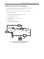
Hardware Components for Non-Contact Imaging ........................................................ 1-65
Summary....................................................................................................................... 1-68
Chapter 2 STM Imaging ..................................................................2-1
Introduction..................................................................................................................... 2-2
Preparing and Loading STM Tips................................................................................... 2-3
Using Wire Cutters to Make STM Tips............................................................ 2-3
Using ThermoMicroscopes’s Tip Etcher........................................................... 2-4
Setting Up the Tip Etcher ................................................................... 2-5
Operating the Tip Etcher .................................................................... 2-6
Using the STM Cartridge.................................................................................. 2-8
Inserting the STM Tip into the STM Cartridge .................................. 2-9
Taking an STM Image .................................................................................................. 2-12
Setting Up the System .................................................................................... 2-13
Setting Up Hardware ........................................................................ 2-13
Configuring the Software ................................................................. 2-14
Diagnostic Checks............................................................................ 2-15
Approaching the Sample................................................................................. 2-17
Setting Up for an Auto Approach..................................................... 2-17
Performing an Auto Approach ......................................................... 2-20
Starting a Scan ................................................................................................ 2-21
Optimizing STM Scan Parameters ................................................................. 2-22
Constant-Current vs. Constant-Height Mode ................................................. 2-23
Taking a Constant-Current Mode Image .......................................... 2-24
Taking a Constant- Height Mode Image .......................................... 2-25
While You Are Taking an STM Image........................................................... 2-25
Taking an STM Image of a Graphite Sample ................................................. 2-26
Summary....................................................................................................................... 2-27
Chapter 3 LFM Imaging ................................................................3-1
Introduction..................................................................................................................... 3-2
How Lateral Force Microscopy (LFM) Works ............................................................... 3-3
The LFM Signal................................................................................................ 3-3
The Tip-Sample Interaction for LFM ............................................................... 3-4
Setting up the System...................................................................................................... 3-8
Installing the Scanner and the Probe Head ....................................................... 3-8
Configuring the Software ............................................................................... 3-10
Contents
Aligning the Deflection Sensor .......................................................................3-10
Troubleshooting Tips ........................................................................3-13
Performing an Auto Approach ........................................................................3-14
Troubleshooting Tips: Approach .....................................................3-14
Taking an LFM Image...................................................................................................3-16
Selecting the LFM Signal................................................................................3-16
Setting Scan Parameters ..................................................................................3-17
Starting a Scan.................................................................................................3-17
Troubleshooting Tips: Signal Saturation .........................................3-18
Summary .......................................................................................................................3-19
Chapter 4 Force vs. Distance ..................................................... 4-1
Introduction .....................................................................................................................4-2
The F vs. d Spectroscopy Window ..................................................................................4-3
The Force vs. Distance Graph ...........................................................................4-4
Spectroscopy Mode Controls ............................................................................4-5
The Piezo Adjustment Bar ..................................................................4-8
Acquiring Force vs. Distance Data..................................................................................4-9
Setting Up to Acquire an F vs. d Curve.............................................................4-9
Taking a Contact-AFM Image ............................................................4-9
Calibrating the Vertical F vs. d Axis.................................................4-11
Generating a Force vs. Distance Curve ...........................................................4-14
Adjusting the Horizontal and Vertical Scales of an F vs. d Curve ..................4-18
Zooming in on a Region of Interest.................................................................4-20
Zooming in Graphically Using the Cursor........................................4-20
Zooming in by Changing the Scanner’s Sweep Range .....................4-21
Making Point-to-Point Measurements on an F vs. d Curve.............................4-22
Generating an F vs. d Curve at a Different X, Y Location..............................4-22
Acquiring F vs. d Curves Along a Line...........................................................4-23
Saving, Exporting, and Printing Data..............................................................4-24
Redisplaying Curves in F vs. d Spectroscopy .................................................4-25
Where to Go From Here ................................................................................................4-26
Forces Acting on the Cantilever ....................................................................................4-27
Understanding Force vs. Distance Curves.....................................................................4-29
Cantilever Data Sheets ..................................................................................................4-31
Microlevers .....................................................................................................4-31
Ultralevers .......................................................................................................4-32
Summary .......................................................................................................................4-33
vii
viii
Chapter 5 I-V Spectroscopy .........................................................5-1
Introduction..................................................................................................................... 5-2
The I-V Spectroscopy Window....................................................................................... 5-3
I-V Spectroscopy Controls.............................................................................................. 5-5
Acquiring Current vs. Voltage Data................................................................................ 5-7
Generating a Current vs. Voltage Curve........................................................... 5-7
Generating an I-V Curve at a Different X, Y Location .................................... 5-9
Adjusting the Horizontal and Vertical Scales of an I-V Curve......................... 5-9
Zooming in on a Region of Interest ................................................................ 5-11
Zooming in Graphically Using the Cursor ....................................... 5-11
Zooming in by Changing the Voltage Sweep Range........................ 5-11
Making Point-to-Point Measurements on an I-V Curve ................................. 5-12
Saving and Exporting Data............................................................................. 5-12
Redisplaying Curves in I-V Spectroscopy...................................................... 5-13
Summary....................................................................................................................... 5-14
Chapter 6 Scanner Calibration....................................................6-1
Introduction..................................................................................................................... 6-2
How the Scanner Works ................................................................................................. 6-3
When to Calibrate the Scanner........................................................................................ 6-4
Calibrating a 5 Micron Scanner ...................................................................................... 6-5
What it Means to Calibrate a 5 Micron Scanner............................................... 6-5
Scanner Calibration Procedures........................................................................ 6-6
Setting Up the System ........................................................................ 6-7
First-Order Calibration of Scanner Sensitivity in X and Y .............. 6-11
Second-Order Calibration of Scanner Sensitivity in X and Y .......... 6-17
Calibration of Scanner Sensitivity in Z ............................................ 6-20
Creating a Backup Scanner Calibration File .................................... 6-23
Calibrating a 100 Micron Scanner ................................................................................ 6-24
How ScanMaster Works ................................................................................. 6-24
What it Means to Calibrate a 100 Micron Scanner......................................... 6-26
Scanner Calibration Procedures...................................................................... 6-27
Installing the System Hardware........................................................ 6-27
Configuring the System Software .................................................... 6-28
Calibrating the XY Detector............................................................. 6-31
Calibrating the Z Detector ................................................................ 6-34
Auto Calibration of Detector Offsets and Scanner Sensitivity ......... 6-36
Creating a Backup Scanner Calibration File .................................... 6-38
Summary....................................................................................................................... 6-40
Preface
Operating Safety
This section includes important information about your AutoProbe CP system. It
describes in detail procedures related to the operating safety of AutoProbe CP and
therefore must be read thoroughly before you operate your AutoProbe CP system.
WARNING!
The protection provided by the AutoProbe CP system may be impaired if the
procedures described in this User’s Guide are not followed exactly.
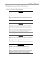
Safety Symbols
Table 0-1 lists symbols that appear throughout this User’s Guide and on the
AutoProbe CP system. You should become familiar with the symbols and their function.
The symbols are used to alert you to matters related to the operating safety of the
AutoProbe CP system.
Table 0-1. Safety symbols and their functions.
Symbol
Function
Direct current source.
Alternating current source.
Direct and alternating current source.
3
Three-phase alternating current.
Ground (earth) terminal.
Protective conductor terminal.
Frame or chassis terminal.
Equipotentiality.
Power on.
x
Preface
Table 0-1 (continued). Safety symbols and their function.
Symbol
Function
Power off.
Equipment protected by double or reinforced insulation.
!
Refer to system documentation.
Electric shock risk.
Definitions: Warning, Caution, and Note
There are three terms that are used in this User’s Guide to alert you to matters related to
the operating safety of AutoProbe CPwarning, caution, and note. These terms are
defined in Table 0-2, below.
Table 0-2. Safety terms and their definitions.
Term
Definition
Warning
Alerts you to possible serious injury unless procedures described in
this User’s Guide are followed exactly. Do not proceed beyond a
warning until conditions are fully understood and met.
Caution
Calls your attention to possible damage to the system or to the
impairment of safety unless procedures described in this User’s Guide
are followed exactly.
Note
Calls your attention to a rule that is to be followed or to an out of the
ordinary condition.
It is important that you read all warnings, cautions, and notes in this manual carefully.
Warnings, cautions, and notes include information that, when followed, ensures the
operating safety of your AutoProbe CP system.
xi
Summary of Warnings and Cautions
This section includes warnings and cautions that must be followed whenever you operate
AutoProbe CP.
WARNING!
AutoProbe CP must be properly grounded before you turn on the power to its
components. The mains power cord must only be inserted into an outlet with a
protective earth ground contact. See the section “Grounding AutoProbe CP”
later in this preface for more information.
WARNING!
The line voltage selection must be checked before you turn on the power to
AutoProbe CP's system components. The line voltage selector switch is on the
rear panel of the AEM. The line voltage selector switch can be set to the
following voltages: 100 V, 120 V, 220 V, and 240 V. See the section “Setting
the Line Voltage” later in this preface for more information.
WARNING!
Do not open the AutoProbe electronics module (AEM) or the CP base unit. The
AEM and the CP base unit use hazardous voltages and therefore present serious
electric shock hazards.
WARNING!
ThermoMicroscopes requires that you routinely inspect the cables of the
AutoProbe CP system to make sure that they are not frayed, loose, or damaged.
Cables that are frayed, loose, or damaged must be immediately reported to your
local ThermoMicroscopes service representative. Do not operate AutoProbe CP
when wires are frayed, loose, or damaged.
xii
Preface
CAUTION
All AutoProbe CP system components must be handled with care. System
components contain delicate electromechanical instrumentation that can easily
be damaged by improper handling.
CAUTION
The power to the AEM must be turned OFF before you remove or install the
scanner.
CAUTION
The LASER ON/OFF switch of the probe head must be in the OFF position
before you remove or install the probe head on the XY translation stage.
Otherwise, damage to the light-emitting diodes (LEDs) of the probe head may
result.
CAUTION
When removing and installing the scanner, you must be grounded via a
grounding strap to ensure that the scanner is not damaged. The scanner is
sensitive to electrostatic discharge.
CAUTION
The four screws that connect the scanner to the CP base unit must be securely
fastened to ensure proper grounding. When the four screws are securely
fastened, maximum instrument performance is ensured since vibrations are
reduced.
xiii
CAUTION
To preserve safety and EMC compliance, AutoProbe CP must be used with the
EMI filter supplied with the AutoProbe CP system.
CAUTION
To preserve EMC immunity, place the metal cover on the CP base unit while
imaging.
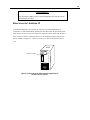
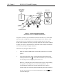
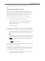
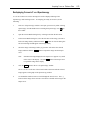
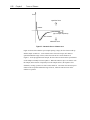
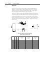
Grounding AutoProbe CP
AutoProbe CP must be properly grounded before you turn on the power to its
components. The mains power cord must be inserted into an outlet with a protective earth
ground contact. If you do not have access to an outlet with a protective earth ground
contact, you must ground the AutoProbe CP system using the ground connection of the
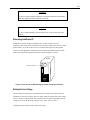
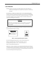
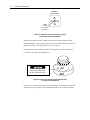
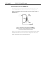
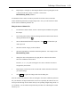
AEM. The location of the ground connection is shown in Figure 0-1, below.
AEM
Ground connection
Figure 0-1. Rear panel of the AEM, showing the location of the ground connection.
Setting the Line Voltage
The line voltage selection must correspond to the line voltage of the country where the
AutoProbe CP system is operated. The line voltage selection is made using a line voltage
selector. The line voltage selector unit is located on the rear panel of the AEM. The line
voltage can be set to the following voltages: 100 V, 120 V, 220 V, or 240 V.
To change the line voltage selection, follow these steps:
xiv
Preface
1.
Make sure the power to the AEM is turned off.
2.
Unplug the AEM’s power cord from the power outlet.
3.
Remove the cover of the line voltage selector unit using an appropriately sized
screwdriver.
4.
Insert an appropriately sized tool into the line voltage selector slot and use the
tool to remove the line voltage selector wheel from the unit.
5.
Set the line voltage on the line voltage selector wheel to the desired value100
V, 110 V, 220 V, or 240 V.
6.
Put the line voltage selector wheel back into its location in the unit. Make sure
that the desired voltage is shown in the window.
7.
Install the cover onto the line voltage selector unit.
The line voltage should now be set to the appropriate value.
xv
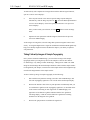
Laser Safety
Note:
Throughout this section, the drawings refer to the AFM probe head for the
standard system configuration of AutoProbe CP unless otherwise noted.
AutoProbe CP contains a diode laser powered by a low voltage supply with a maximum
output of 0.2 mW CW in the wavelength range 600 to 700 nm. Diode laser power up to
0.2 mW at 600 to 700 nm could be accessible in the interior. AutoProbe CP should
always be operated with the probe head properly installed.
WARNING!
Use of controls or adjustments or performance of procedures other than those
specified herein could result in hazardous laser light exposure.
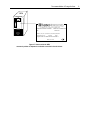
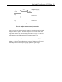
Figure 0-2 shows the two laser warning labels of the probe head. Strict observance of
these laser warning labels is required.
CAUTION
LASER LIGHT DO NOT STARE INTO BEAM
0.2 mW AT 600-700 nm
CLASS II LASER PRODUCT
CLASS 2
PER EN60825-1 1994
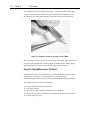
Figure 0-2. Laser warning labels of the probe head.
The left warning label in Figure 0-2, above, specifies that the probe head is a
Class II laser product per 21 CFR 1040.10 and 1040.11. The right warning label in
Figure 0-2, above, specifies that the scanning head is a Class 2 laser product per
EN60825.
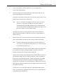
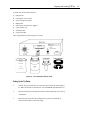
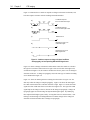
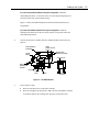
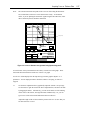
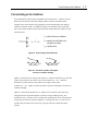
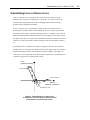
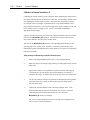
Figures 0-3 through 0-7 below show the location of all instrument controls and indicators
pertaining to laser operation for AutoProbe CP systems. They also show the locations of
all laser safety warning labels, the aperture label, and the compliance label.
xvi
Preface
laser
intensity
indicators
laser
position
indicators
laser power
on/off switch
video display
laser beam
steering screws
On
Off
green
prism
PSPD
up/down
PSPD
forward/
backward
CAUTION
LASER LIGHT DO NOT STARE INTO BEAM
AVOID EXPOSURE
LASER LIGHT IS
EMITTED FROM
THIS APERTURE
0.2 mW AT 600-700 nm
CLASS II LASER PRODUCT
CLASS 2
PER EN60825-1 1994
Figure 0-3. Location of laser controls, indicators, and labels on the probe head.
The controls and indicators shown above in Figure 0-3 have the following functions:
Laser power on/off switch: Turns the laser in the probe head on or off. A red light in the
switch is lit when the laser power is on.
Laser beam steering screws: The two laser beam steering screws located on the top right
side of the probe head are used to adjust the position of the laser beam hitting the
cantilever. The screws move the laser spot in two directions, as shown in Figure 0-3,
above. If your system includes the optional CP optics, you can monitor these adjustments
using the optical view displayed on your video monitor.
PSPD adjustment screws: There are two PSPD (position-sensitive photodetector) screws
on the probe headup/down and forward/backward. These screws adjust the position of
the PSPD in the probe head to center the reflected laser light on the photodetector. The
forward/backward adjustment screw is useful for PSPD alignment on all probe heads.
The up/down adjustment is useful primarily for the AFM/LFM probe head of the
standard system configuration.
Laser intensity indicators: Indicates the intensity of reflected laser light hitting the PSPD.
For the standard configuration, there are three probe heads that require laser intensity
indicatorsAFM, AFM/NC-AFM, and AFM/LFM. There are different indicators for the
different probe heads.
xvii
Note:
The AFM probe head comes with the standard system configuration. The
AFM/NC-AFM and AFM/LFM probe heads can be purchased separately for the
standard system configuration.
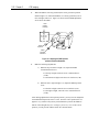
The indicators for the AFM probe head are shown in Figure 0-3, above. For this probe
head, the intensity of laser light hitting the PSPD is maximized when the column of four
red lights is lit. The indicators for the AFM/NC-AFM and AFM/LFM probe heads are
shown in Figure 0-4, below. For these probe heads, when the brightness of the center
green light (which has variable brightness) is maximized, the laser intensity hitting the
PSPD is maximized.
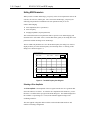
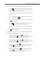
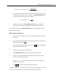
laser intensity and position indicators
for other probe heads
AFM/NC-AFM
probe heads
green
(analog
for variable
brightness)
AFM/LFM
probe heads
green
(analog
for variable
brightness)
Figure 0-4. Laser intensity and position indicators for the AFM/NC-AFM and AFM/LFM probe
heads of the standard system configuration.
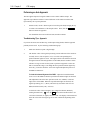
For the multitask configuration, when the brightness of the center green light (which has
variable brightness) is maximized, the laser intensity hitting the PSPD is maximized. See
Figure 0-5, below.
Multitask
probe heads
green
(analog
for variable
brightness)
Figure 0-5. Laser intensity and position indicators for the multitask probe head.
xviii Preface
Laser position indicators: Indicate the position of the reflected laser light hitting the
PSPD. When the laser spot is centered on the photodetector, the center green light is lit,
as shown in Figures 0-4 and 0-5, above.
Figure 0-6, below, shows the location of the laser warning labels on the outer housing of
AutoProbe CP.
CAUTION
LASER LIGHT WHEN OPEN
DO NOT STARE INTO BEAM
Figure 0-6. Laser warning location on AutoProbe CP housing.
Figure 0-7, below, shows the location of the laser safety compliance label on the rear
panel of the AutoProbe electronics module (AEM).
AEM
1171 Borregas Ave. Sunnyvale, CA 94089-1304
AutoProbe Electronics Module
Model No. APEM-1000
Serial No.
Date
Patents 5,157,251 5,210,410 5,376,790,5,448,399
100/120/220/240 VAC
50/60 Hz
400W
Complies with 21 CRR 1040.10 and1040.11
Made in the USA
Figure 0-7. Rear panel of the AEM,
showing location of laser safety compliance label.
xix
Specifications and Performance for AutoProbe CP
System Configurations:
Standard
Includes an AFM probe head for operation in
AFM mode.
Optional AFM/NC-AFM probe head can be
purchased for operation in AFM, non-contact AFM,
intermittent-contact AFM, and MFM modes.
Optional AFM/LFM probe head can be purchased
for operation in AFM and LFM modes.
Optional STM toolkit can be purchased for
operation in STM mode.
Multitask
Includes a multitask probe head for operation in the
following modes: contact, non-contact, and
intermittent-contact AFM, MFM, LFM, and STM.
Measurement Performance:
Standard:
Scanner
5 µm piezoelectric scanner.
Scan range
Maximum lateral scan range: 5 µm.
Maximum vertical scan range: 2.5 µm.
Control resolution
Maximum lateral resolution: 0.0013 Å.
Maximum vertical resolution: 0.009 Å.
Multitask:
Scanner
100 µm piezoelectric scanner.
Scan range
Maximum lateral scan range: 100 µm.
Maximum vertical scan range: 7.5 µm.
Control resolution
Maximum lateral resolution: 0.25 Å.
Maximum vertical resolution: 0.025 Å.
Microscope Stage:
Translation range
8 mm x 8 mm.
Sample size
50 mm (w) x 50 mm (l) x 25 mm (h) for the standard
configuration.
50 mm (w) x 50 mm (l) x 20 mm (h) for the multitask
configuration.
Tip-to-sample approach
Automatic with 3 independent stepper motors.
Optical microscope
Optional on-axis microscope with color video
monitor for probe tip and sample view.
5:1 zoom, up to 3,500X magnification.
Acoustic isolation
Optional acoustic isolation chamber.
xx
Preface
Workstation:
AEM
20-bit DACs for x, y, and z axes.
16-bit DACs for system control.
Computer
100 MHz Pentium processor, 256 Kbyte cache
memory, 16 MB RAM.
Mass storage
Software
1 GB hard drive, 3 1/2 in. 1.4 MB floppy disk drive.
ProScan Data Acquisition and Image Processing
operates under Windows 95.
Graphics
Windows graphics accelerator, 17 in.
high-resolution color monitor.
System power
115/230 V AC, 50/60 Hz, 600 W.
Dimensions and Weights:
CP base unit
10.5 in. (267 mm) x 8 in. (203 mm); 22 lb (10 kg).
AEM
17 in. (432 mm) x 7 1/2 in. (191 mm) x
17 1/2 in. ( 445 mm); 43 lb (20 kg).
Computer
17 in. (432 mm) x 7 1/2 in. (191 mm) x
17 1/2 in. ( 445 mm); 27 lb (12 kg).
Operating Environment:
Temperature
0°C to 30°C, 32°F to 112°F.
Humidity
90%; noncondensing.
Cleaning Agents:
CP base unit
Isopropyl alcohol.
Probe head
Isopropyl alcohol.
AEM and computer
Isopropyl alcohol.
WARNING!
To avoid risk of electric shock, do not clean AutoProbe CP system components
when power to the components is turned on.
CAUTION
Do not use acetone to clean AutoProbe CP system components. Acetone may
damage important safety warning labels.
xxi
ThermoMicroscopes Warranty Statement
Warranty on New Systems and Accessories
ThermoMicroscopes warrants to the original purchaser of the equipment that the
equipment will be free from defects in material and workmanship for a period of one year
from date of delivery. ThermoMicroscopes agrees as its sole responsibility under this
limited warranty that it will replace or repair, at its option, the warranted equipment at no
charge to the purchaser and will perform services either at ThermoMicroscopes’s facility
or at the customers facility, at ThermoMicroscopes’s option. For repairs performed at
ThermoMicroscopes’s facility, the customer must contact ThermoMicroscopes in advance
for authorization to return the equipment and must follow ThermoMicroscopes’s shipping
instructions. If returned, the equipment must be insured.
ThermoMicroscopes will supply replacement parts on loan, whenever possible, to enable
field repair by customers with minimum downtime; once the system is operational the
defective parts are then returned to ThermoMicroscopes.
Specifically excluded from this warranty are all consumable parts including, but not
limited to, Microlevers, Ultralevers, and tips. The warranty of equipment sold for use
outside the United States depends on the condition of each sale. Equipment which has
been subjected to misuse, accident, abuse, disaster, unreasonable use, damage caused by
third party systems with which the equipment is used, operational error, neglect,
unauthorized repair, alteration or installation is not covered by this warranty.
Warranty on Replacement Parts
ThermoMicroscopes warrants all replacement parts to be sold free from defects in
materials or workmanship for a period of 90 days from the date received by the customer.
ThermoMicroscopes will repair or replace, at its discretion, such parts when returned to
ThermoMicroscopes. Customers must contact ThermoMicroscopes in advance to obtain
authorization to return parts and follow ThermoMicroscopes’s shipping instructions.
Except as herein provided, seller makes no warranties, express or implied, and seller
expressly excludes and disclaims any warranty of merchantability or fitness for a
particular purpose. Under no circumstances shall ThermoMicroscopes be liable for any
loss or damage, direct, special, indirect or consequential, arising from the use or loss of
use of any product, service, part, supplies or equipment. Nor shall ThermoMicroscopes
be liable under any legal theory, including, but not limited to, lost profits, down-time,
goodwill, damage to or replacement of equipment or property, and any cost of
recovering, reprogramming, or reproducing any program or data stored in or used with
ThermoMicroscopes products.
xxii
Preface
Some states do not allow limitations on the period of time an implied warranty lasts
and/or the exclusion or limitation of special, incidental or consequential damages, so the
above limitations and/or exclusions may not apply to you. This warranty gives you
specific legal rights, and you may also have other rights which vary from state to state.
Manufacturer Information
AutoProbe CP systems contain no user serviceable parts. All service issues should be
addressed to your local ThermoMicroscopes representative.
ThermoMicroscopes, USA
ThermoMicroscopes, USA
1171 Borregas Avenue
6 Denny Road, No. 109
Sunnyvale, CA 94089
Wilmington, DE 19809
T: (408) 747-1600
T: (302) 762-2245
F: (408) 747-1601
F: (302) 762-2847
ThermoMicroscopes, SA
ThermoMicroscopes, Korea
16 rue Alexandre Gavard
Suite 301, Seowon Building
1227 CAROUGE
395-13, Seokyo-dong, Mapo-ku
Geneva, Switzerland
Seoul, Korea
T: 41-22-300-4411
T: 82-2-325-3212
F: 41-22-300-4415
F: 82-2-325-3214
If you return system components to ThermoMicroscopes for service that have come into
contact with harmful substances you must observe certain regulations. Harmful
substances are defined by European Community Countries as "materials and preparations
in accordance with the EEC Specification dated 18 September 1979, Article 2." For
system components that have come into contact with harmful substances, you must do the
following:
♦
Decontaminate the components in accordance with the radiation protection
regulations.
♦
Construct a notice that reads "free from harmful substances.” The notice must be
included with the components and the delivery note.
xxiii
How to Use This User’s Guide
The User’s Guide to AutoProbe CP is divided into three, easy-to-use parts. The parts
include the following:
♦
Part I: Learning to Use AutoProbe CP: Basic Imaging Techniques
♦
Part II: Learning to Use AutoProbe CP: Advanced Techniques
♦
Part III: Software Reference
The contents of the above-listed parts are described in detail in the sections below.
Part I: Learning to Use AutoProbe CP: Basic Imaging Techniques
Part I of this User’s Guide, Learning to Use AutoProbe CP: Basic Imaging Techniques,
contains an introductory chapter and three hands-on tutorials, Chapters 2 through 4. By
working through the tutorial chapters, you will learn the basic skills needed to set up the
instrument and to take an AFM image.
Start by reading Chapter 1, "AutoProbe CP Basics," for an introduction to the system
configurations and the components of AutoProbe CP. Then, work through the tutorial in
Chapter 2, "Setting Up to Take an Image" to learn how to set up the system hardware and
software for AFM mode. More specifically, you will learn the procedures for connecting
cables, removing and installing a probe head and a scanner, and loading a sample and a
probe.
Chapter 3, "Taking an AFM Image," guides you through setting up the system software,
approaching the sample, and taking an AFM image. Chapter 4, "Taking Better Images,"
teaches you how to optimize scan and feedback parameters to take higher quality images
and how to save and retrieve images.
Part II: Learning to Use AutoProbe CP: Advanced Techniques
Part II of this User’s Guide, Learning to Use AutoProbe CP: Advanced Techniques,
includes hands-on tutorials for operation in the following modes: NC-AFM, IC-AFM,
MFM, STM, and LFM. It also includes tutorials that introduce you to advanced
capabilities of AutoProbe CP, such as force vs. distance and current vs. voltage data
acquisition, and scanner calibration.
Chapter 1, "NC-AFM, IC-AFM, and MFM Imaging," provides step-by-step instructions
for taking NC-AFM, IC-AFM, and MFM images. Chapter 1 also describes the principles
behind NC-AFM, IC-AFM, and MFM modes of operation.
xxiv Preface
Chapter 2, "STM Imaging," guides you through taking an STM image. In this chapter,
you learn procedures for preparing an STM tip and using a STM cartridge, setting up the
hardware and software for operation in STM mode, and taking an STM image.
Chapter 3, "LFM Imaging," leads you through taking simultaneous LFM and AFM
images. Chapter 3 also includes information on how LFM images are produced and the
usefulness of having both LFM and AFM images available.
Chapter 4, "Force vs. Distance Curves," describes how to use the F vs. D Spectroscopy
window of ProScan Data Acquisition to generate force vs. distance curves at x, y
locations on the sample surface. A force vs. distance curve is a plot of the vertical force
that the tip applies to the cantilever as a function of the tip-to-sample distance. Variations
in the shape of force vs. distance curves provide information about the local elastic
properties of the sample surface.
Chapter 5, "I-V Spectroscopy," teaches you how to use the I-V Spectroscopy window of
ProScan Data Acquisition to generate current vs. voltage (I-V) and dI/dV curves. These
curves are used to provide important information about surface electronic properties.
Chapter 6, "Scanner Calibration," describes how the scanner of your AutoProbe CP
instrument works and how to calibrate it to maintain its optimal performance.
Part III: Software Reference
Part III of this User’s Guide, Software Reference, is the reference manual for ProScan
Data Acquisition and Image Processing and includes information for the following
AutoProbe systems: CP, LS, and M5. The chapters in this part of the User’s Guide
provide more detailed information about the software features and controls than the
information that is provided in the tutorial chapters. The chapters are designed so that
you can skip straight to the feature or control that you are interested in learning more
about.
Chapter 1, "ProScan Data Acquisition," describes in detail the software features of
ProScan Data Acquisition. This chapter discusses each region of the screen, giving
special attention to each control and its function. This chapter also discusses the menus,
with a description of each menu item and its function.
Chapter 2, "ProScan Image Processing," describes in detail the software features of
ProScan Image Processing. This chapter explains how to process images, how to make
surface measurements, and how to prepare images for printout in a variety of formats.
Vorwort
Betriebssicherheit
Dieses Kapitel enthält wichtige Informationen über ihr AutoProbe CP System. Es
beschreibt im Detail den Arbeitsablauf in Bezug auf die Betriebssicherheit des AutoProbe
CP und muss daher vollständig durchgelesen werden bevor sie ihr AutoProbe CP System
bedienen.
WARNUNG!
Der durch das AutoProbe CP System versehene Schutz ist beeinträchtigt, falls
die in diesem Benutzerhandbuch beschriebenen Arbeitsabläufe nicht genaustens
befolgt werden.
Sicherheits Zeichen
In Tabelle 0-1 sind die im Benutzerhandbuch und auf dem AutoProbe CP System
vorkommenden Zeichen aufgelistet. Sie sollten mit der Wirkung der Zeichen vertraut
werden, in welcher Weise sie mit der Betriebssicherheit des AutoProbe CP in
Zusammnehang stehen.
Tabelle 0-1. Sicherheits Zeichen und ihre Wirkung.
Zeichen
Wirkung
Gleichstromquelle.
Wechselstromquelle.
Wechselstrom- und Gleichstromquelle.
3
Dreiphasenstromquelle.
Erdungsanschluss.
Schutzerdungsanschluss.
Gehäuse- oder Rahmenanschluss.
Äquipotentialanzeige.
Schaltet Stromversorgung ein.
xxvi Vorwort und Übersicht
Tabelle 0-1(Fortsetzung). Sicherheits Zeichenund ihre Wirkung.
Zeichen
Wirkung
Schaltet Stromversorgung aus.
Bezeichnet doppelte oder verstärkte Isolierung des Gerätes.
!
Weisst den Benutzer auf eine in der Dokumentation enthaltene
Information hin.
Zeigt eine Berührungsgefahr an.
Definitionen: Warnung, Vorsicht und Beachte
Im Benutzerhandbuch werden drei verschiedene Bezeichnungen, Warnung, Vorsicht und
Beachte, benutzt, um auf die Betriebssicherheit des AutoProbe CP hinzuweisen. Diese
Bezeichnungen sind in Tabelle 0-2 definiert.
Tabelle 0-2. Sicherheits Bezeichnungen und ihre Definition.
Bezeichnung
Definition
Warnung
Warnt vor möglicher ernsthafter Verletzungsgefahr, falls dem im
Benutzerhandbuch beschriebenen Arbeitsablauf nicht unbedingt
Folge geleistet wird. Der Arbeitsablauf darf nicht fortgeführt
werden, bis nicht alle Voraussetzungen verstanden und erfüllt sind.
Vorsicht
Macht auf mögliche Schädigung des Systems oder
Verschlechterung der Sicherheit aufmerksam, falls dem im
Benutzerhandbuch beschriebenen Arbeitsablauf nicht unbedingt
Folge geleistet wird.
Beachte
Macht auf eine zu beachtende Benutzungsregel oder ungewöhnliche
Voraussetzung aufmerksam.
Es ist wichtig, dass alle Warnungen, Vorsichts, und Beachte in diesem Handbuch
achtsam gelesen werden, um die Bedienungssicherheit ihres AutoProbe CP Systems zu
gewährleisten.
Betriebssicherheit xxvii
Zusammenfassung der Warnungen und Vorsichts
Dieser Abschnitt beinhaltet die Warnungen und Vorsichts, die unbedingt befolgt werden
müssen, wann immer das AutoProbe CP betrieben wird.
WARNUNG!
Das AutoProbe CP muss ordnungsgemäss geerdet werden, bevor Spannung an
seine Komponenten angelegt werden darf. Das Versorgungskabel darf nur mit
einen Anschluss verbunden werden, der mit einem Erdungspol versehen ist. Für
weitere Informationen soll der Teil “Erdung des AutoProbe CP” folgend in
diesem Vorwort beachtet werden.
WARNUNG!
Vor dem Einschalten der AutoProbe CP Systemkomponenten muss der
Versorgungsspannungsschalter überprüft werden. Der Versorgungsspannungsschalter befindet sich an der Rückwand des AEM und kann folgendermassen
eingestellt werden: 110 V, 120 V, 220 V und 240 V. Für weitere Informationen
soll der Teil “Einstellen der Versorgungsspannung” folgend in diesem Vorwort
beachtet werden.
WARNUNG!
Das AutoProbe Elektronik Modul (AEM) oder die CP Grundeinheit dürfen nicht
geöffnet werden. Das AEM und die CP Grundeinheit führen Hochspannung,
welche bei Freilegung zu ernsthaften Verletzungen führen kann..
WARNUNG!
ThermoMicroscopes verlangt eine routinemässige Überprüfung der Kabel des
AutoProbe CP Systems um sicherzustellen, dass sie nicht durchgescheuert, lose
oder beschädigt sind.. Kabel welche durchgescheuert, lose oder beschädigt sind,
müssen augenblicklich dem örtlichen ThermoMicroscopes Servicevertreter
gemeldet werden. Das AutoProbe CP soll nicht benutzt werden, falls Kabel
durchgescheuert, lose oder beschädigt sind.
xxviii Vorwort und Übersicht
VORSICHT!
Alle AutoProbe CP Systemkomponenten müssen mit Vorsicht behandelt
werden. In den Systemkomponenten befinden sich empfindliche
elektromechanische Messgerätausrüstungen welche bei unsachgemässer
Behandlung beschädigt werden können.
VORSICHT!
Um eine Berührungsgefahr zu vermeiden muss beim Entfernen und Installieren
des Scanners die Spannung des AEM immer ausgeschaltet sein.
VORSICHT!
Der LASER ON/OFF Schalter des Tastkopfes muss immer ausgeschaltet (OFF
Stellung) sein, bevor der Tastkopf entfernt oder an der XY -Bühne installiert
wird. Bei Nichtbefolgen des letzteren können die Laserdioden (LEDs) des
Tastkopfes beschädigt werden.
VORSICHT!
Um ein beschädigen des Scanners zu vermeiden. müssen sie beim Entfernen und
Installieren des Tastkopfesopfes über ein Erdungskabel geerdet sein. Der
Tastkopf ist sehr empfindlich gegen elektromagnetische Entladungen.
VORSICHT!
Um eine ordungsgemässe Erdung des CP Scanners zu gewährleisten, müssen die
vier Schrauben die den Scanner mit der CP Grundeinheit verbinden, sicher
angezogen werden. Wenn die vier Schrauben sicher angezogen sind, ist eine
maximale Instrumentenauflösung gewährleistet, da die Vibrationen reduziert
sind.
Betriebssicherheit xxix
VORSICHT!
Um die EMV Beständigkeit zu gewährleisten, sollte während dem Aufnahmen
die CP Grundeinheit mit dem metallenen Deckel geschlossen werden.
Erdung des AutoProbe CP
Das AutoProbe CP muss ordungsgemäss geerdet werden, bevor seine Komponenten
eigeschaltet werden. Das Versorgungskabel darf nur mit einen Anschluss verbunden
werden, der mit einem Erdungspol versehen ist. Falls sie keinen Anschluss mit einem
Erdungspol haben müssen sie das AutoProbe CP System über den Erdungspol am AEM
mit Erde verbinden. Die Position des Erdungspoles is im folgenden Bild 0-1
eingezeichnet.
AEM
Ground connection
Bild 0-1. Rückwand des AEM, zeigt die Position des Erdungspoles.
xxx
Vorwort und Übersicht
Einstellen der Versorgungsspannung
Die Einstellung der Versorgungsspannung muss mit der Versorungsspannung des Landes
übereinstimmen, in dem das AutoProbe M5 betrieben wird. Die Einstellung erfolgt über
einen Spannungs-Wahl-Schalter, der sich an der Rückseite des AEM befindet. Die
Spannung kann folgendermassen eingestellt werden: 100V, 120V, 220V oder 240V.
Um die Einstellung der Versorgungsspannung zu ändern, müssen folgende Schritte
befolgt werden:
1.
Versichern sie sich, dass die Spannung des AEM ausgeschaltet ist.
2.
Stecken sie das Versorgungskabel des AEM aus.
3.
Entfernen sie die Abdeckung der Spannung-Wahl-Schalter-Einheit mit Hilfe
eines passenden Schraubenziehers.
4.
Führen sie ein passendes Werkzeug in den Schlitz des Spannung-Wahl-Schalters
und lösen sie mit dessen Hilfe das Spannungs-Wahl-Rad aus der Einheit.
5.
Stellen sie das Spannungs-Wahl-Rad in der benötigte Spannung ein; 100V,
120V, 220V oder 240V.
6.
Stecken sie das Spannungs-Wahl-Rad zurück in seine Position in der Einheit.
Versichern sie sich, dass die gewählte Spannung im Fenster sichtbar ist.
7.
Befestigen sie die Abdeckung über der Spannungs-Wahl-Schalter-Einheit.
Die Versorgungsspannung sollte nun ordnungsgemäss eingestellt sein.
Betriebssicherheit xxxi
Laser Sicherheit
Beachte: In diesem Teil beziehen sich alle Darstellungen auf den AFM Tastkopf der
standard system Konfiguration des AutoProbe CP, ansonsten ist es anderwertig
bezeichnet.
Das AutoProbe CP enthält eine Laserdiode welche von einer Niederspannungsquelle
betrieben wird und eine maximalen Arbeitsleistung von 0.2 mW CW in der Wellenlänge
600-700 nm hat. Im innern des Gerätes könnte eine Diodelaserleistung bis zu 0.2 mW bei
600-700 nm zugänglich sein. Das AutoProbe CP sollte nur bedient werden wenn der
Scanner-Kopf ordnungsgemäss montiert ist.
WARNUNG!
Die Benutzung von Steuerungen, Reglern oder das Ausführen von Verfahren
anders als bis hierhin beschrieben, kann zu Freisetzung von gefährlichem
Laserlicht führen.
Bild 0-2 zeigt die zwei Laserwarnungsmarkierungen des Tastkopfes Strickte Beachtung
dieser Warnungsmarkierungen ist erwartet:
CAUTION
LASER LIGHT DO NOT STARE INTO BEAM
0.2 mW AT 600-700 nm
CLASS II LASER PRODUCT
CLASS 2
PER EN60825-1 1994
Bild 0-2. Laserwarnungsmarkierungen des Tastkopfes.
Die linke Warnungsmarkierung in Bild 0-2, oben, stuft den Tastkopf als ein
Klasse II Laserprodukt nach 21 CFR 1040.10 und 1040.11 ein. Die
Warnungsmarkierung in Bild 0-2, oben, , stuft den Tastkopf als ein
Klasse 2 Laserprodukt nach EN60825 ein.
Bild 0-3 bis 0-7 unten, bezeichnen die Orte aller Instrumentensteuerungen und Anzeiger
im Zusammenhang der Laserbedienung des AutoProbe CP Systems. Weiter werden auch
die Orte der Lasersicherheitskennzeichnungen, der Srahlenöffnungskennzeichnungen und
der Übereinstimmungskennzeichnungen angezeigt.
xxxii Vorwort und Übersicht
laser
intensity
indicators
laser
position
indicators
laser power
on/off switch
video display
laser beam
steering screws
On
Off
green
prism
PSPD
up/down
PSPD
forward/
backward
CAUTION
LASER LIGHT DO NOT STARE INTO BEAM
AVOID EXPOSURE
LASER LIGHT IS
EMITTED FROM
THIS APERTURE
0.2 mW AT 600-700 nm
CLASS II LASER PRODUCT
CLASS 2
PER EN60825-1 1994
BILD 0-3. Ort der Lasersteuerung des Tastkopfes.
Die Steuerungen und Anzeigen, bezeichnet in Bild 0-3, oben, haben folgende
Funktionen:
Laser power on/off switch: Schaltet den Laser des Tastkopfes ein oder aus. Ein rotes
Licht im Schalter leuchtet auf, falls der Laser eingescchaltet ist.
Laser beam steering screws: Die zwei Laserstrahl-Steuerungsschrauben, welche sich
oben and der rechten Seite des Tastkopfes befinden, dienen zur justierung der Position
des Aufteffpunktes des Laserstrahles auf den Balken. Die Schrauben bewegen den
Laserpunkt in zwei Richtungen, wie in Bild 0-3, oben, gezeigt wird. Falls ihr System die
zusätzliche CP Optics enthält, können sie diese Justierung überwachen indem sie die
optische Ansicht auf ihrem Videobildschirm darstellen.
PSPD adjustment screws: Am Tastkopf befinden sich zwei PSPD Schrauben auf/ab
und forwärts/rückwärts. Diese Schrauben justieren die Position des PSPD’s im Tastkopf
um das reflektierte Laserlicht auf dem Photodetektor zu zentrieren. Die forwärts/rückwärts Justierungsschraube kann an allen Tastköpfen zur PSPD-Einstellung benutzt
werden. Die auf/ab Justierung kann hauptsächlich für den AFM/LFM Tastkopf der
Standardkonfiguration benutzt werden.
Laser intensity indicators: Zeigt die Intensität des reflektierten Laserlichtes das auf den
PSPD (Positions-sensiblen Photodetektor) trifft an.
Betriebssicherheit xxxiii
Es gibt drei Tastköpfe für die Standardkonfiguration, AFM, AFM/NC-AFM,
AFM/LFM. Die verschiedenen Tastköpfe haben verschiedene Indikatoren.
Beachte: Der AFM Tastkopf kommt mit der Standardsystemkonfiguration. Die
AFM/NC-AFM und AFM/LFM Tastköpfe sind zusätzlich zur Standardsystemkonfiguration erhältlich.
Die Indikatoren des AFM Tastkopfes sind in Bild 0-3, oben, eingezeichnet. Bei diesem
Tastkopf ist die maximale Laserlichtintensität, die die PSPD teffen kann, erreicht, wenn
die Reihe der vier roten Lichter erleuchtet ist. Die Indikatoren der AFM/NC-AFM und
AFM/LFM Tastköpfe sind in Bild 0-4, unten, eingezeichnet. Bei diesen Tastköpfen ist
die maximale Laserlichtintensität, die die PSPD teffen kann, erreicht, wenn die Helligkeit
des mittleren grünen Lichtes (welches eine veränderliche Helligkeit aufweisst) maximal
ist.
laser intensity and position indicators
for other probe heads
AFM/NC-AFM
probe heads
green
(analog
for variable
brightness)
AFM/LFM
probe heads
green
(analog
for variable
brightness)
Bild 0-4. Laserintensität und Position des Indikators
der AFM/NC-AFM und AFM/LFM Tastköpfe der
Standardsystemkonfiguration.
Bei der Multitaskkonfiguration, ist die maximale Laserlichtintensität, die die PSPD teffen
kann, erreicht, wenn die Helligkeit des mittleren Lichtes (welches eine veränderliche
Helligkeit aufweisst) maximal ist. Eingezeichnet in Bild 0-5, unten.
xxxiv Vorwort und Übersicht
Multitask
probe heads
green
(analog
for variable
brightness)
Bild 0-5. Laserintensität und Position des Indikators des Multitasktastkopfes.
Laser position indicators: Zeigen die Position des reflektierten Laserlichtes, das die
PSPD trifft, an. Wenn der Laserpunkt auf dem Photodetektor zentriert ist, leuchtet das
mittlere grüne Licht auf, wie in Bild 0-4 und 0-5, oben, gezeigt wird.
Bild 0-6, unten, zeigt den Ort der Laserwarnungsmarkierungen auf dem äusseren
AutoProbe CP Gehäuse an.
CAUTION
LASER LIGHT WHEN OPEN
DO NOT STARE INTO BEAM
Bild 0-6. Laserwarnungsort des AutoProbe CP Gehäuses.
Bild 0-7, unten, zeigt den Ort der Lasersicherheitsübereinstimmungskennzeichnung auf
der Rückseite des AutoProbe Elektronic Modules (AEM) an.
Betriebssicherheit xxxv
AEM
1171 Borregas Ave. Sunnyvale, CA 94089-1304
AutoProbe Electronics Module
Model No. APEM-1000
Serial No.
Date
Patents 5,157,251 5,210,410 5,376,790,5,448,399
100/120/220/240 VAC
50/60 Hz
400W
Complies with 21 CRR 1040.10 and1040.11
Made in the USA
Bild 0-7. Rückseite des AEM,
den Ort der Lasersicherheitsübereinstimmungskennzeichnung anzeigend.
xxxvi Vorwort und Übersicht
Spezifikationen und Ausführungen des AutoProbe CP’s
System Ausführungen:
Standard
Beinhaltet einen AFM Tastkopf für Tätigkeit in der
AFM Betriebsart.
Ein AFM/NC-AFM Tastkopf für Tätigkeit in AFM,
berührungsfreies AFM, periodisch kontaktierendes
AFM, und MFM Betriebsarten ist zusätzlich
erhältlich.
Ein AFM/LFM Tastkopf für Tätigkeit in AFM und
LFM Betriebsarten ist zusätzlich erhältlich.
Ein STM Werkzeugset für Tätigkeit in STM
Betriebsart ist zusätzlich erhältlich.
Multitask
Beinhaltet einen Multitasktastkopf für Tätigkeit in
den folgenden Betriebsarten: berührendes,
berührungsfreies, und periodisch kontaktierendes
AFM, MFM, LFM und STM.
Messleistung:
Standard:
Scanner
5 µm piezoelektrischer Scanner.
Scannreichweite
Maximale laterale Scannreichweite: 5 µm.
Maximale verticale Scannreichweite: 2.5 µm.
Reglerresolution
Maximale Lateralresolution: 0.0013 Å.
Maximale Verticalresolution: 0.009 Å.
Multitask:
Scanner
100 µm piezoelectrischer Scanner.
Scannreichweite
Maximale laterale Scannreichweite: 100 µm.
Maximale verticale Scannreichweite: 7.5 µm.
Reglerresolution
Maximale Lateralresolution: 0.25 Å.
Maximale Verticalresolution: 0.025 Å.
Über den Gebrauch des Benutzerhandbuches xxxvii
Mikroscopbühne:
Verschiebbarkeit
8 mm x 8 mm.
Probengrösse
50 mm (w) x 50 mm (l) x 25 mm (h) für die
Standardkonfiguration.
50 mm (w) x 50 mm (l) x 20 mm (h) für die
Multitaskkonfiguration.
Spitze-zu-Probe Einfahrt
Automatisch mit 3 unabhängigen Schrittmotoren.
Optisches Mikroscop
Zusätzliches axiales Mikroscop mit
Farbvideobildschirm zur Ansicht von
Messfühlerspitze und Probe.
5:1 Zoom, bis zu 3,500X Vergrösserung.
Akustische Isolation
Zusätzliche akustische Isolationskammer.
Arbeitsplatz:
AEM
20-bit DACs für x, y, und z Achsen..
16-bit DACs für Systemüberwachung.
Computer
100 MHz Pentium Prozessor, 256 Kbyte
Cachespeicher 16 MB RAM.
Massenspeicher
1 GB Hard Drive, 3 1/2 in. 1.4 MB Floppydisk
Drive..
Software
ProScan Data Acquisition und Image Processing
arbeitets mit Windows 95.
Graphik
Windows Graphikbeschleuniger, 17 in.
hochauflösender Farbmonitor.
Systemspannungen
115/230 V AC, 50/60 Hz, 600 W.
Dimensionen und Gewicht:
CP Grundeinheit
10.5 in (267 mm) x 8 in (203 mm); 22 lb (10 kg).
AEM
17 in (432 mm) x 7 1/2 in (191 mm) x
17 1/2 in ( 445 mm); 43 lb (20 kg).
Computer
17 in (432 mm) x 7 1/2 in (191 mm) x
17 1/2 in ( 445 mm); 27 lb (12 kg).
Betriebssumgebung:
Temperatur
0°C bis 30°C, 32°F bis 112°F;
Luftfeuchtigkeit
90%; nicht kondensierend.
Reinigungsmittel:
CP Grundeinheit
Isopropylalkohol.
Messkopf
Isopropylalkohol.
AEM und computer
Isopropylalkohol.
xxxviiiVorwort und Übersicht
WARNUNG!
Um eine Berührungsgefahr zu vermeiden sollen während dem Reinigen der
AutoProbe CP Systemkomponenten diese immer ausgeschaltet sein.
VORSICHT
Es sollte kein Aceton verwendet werden um die Komponenten des AutoProbe
CP Systems zu reinigen, da dabei wichtige Sicherheits Warnungs Etiketten von
den Komponenten losgelöst werden könnten.
Über den Gebrauch des Benutzerhandbuches xxxix
ThermoMicroscopes Garantieerklährung
Garantie von neuen Systemen und Zubehörteile
ThermoMicroscopes garantiert dem Orginalkäufer des Gerätes, das dieses frei von
Material- und Verarbeitungsfehlern ist. Diese Garantie gilt für ein Jahr ab dem
Lieferdatum. ThermoMicroscopes übernimmt die Verantwortung, das Gerät, welches
unter diese begrenzte Garantie fällt, nach eigenem Ermessen zu reparieren oder zu
ersetzen, ohne Kosten für den Käufer. Alle Serviceleistungen werden je nach ermessen
von ThermoMicroscopes in ThermoMicroscopes Niederlassungen oder beim Kunden
durchgeführt. Bei Reparaturen, welche in ThermoMicroscopes Niederlassungen
durchgeführt werden, muss ThermoMicroscopes vorzeitig kontaktiert werden, um eine
Genehmigung für die Rücksendung des Grätes zu erhalten. Für den Transport des Gerätes
muss den ThermoMicroscopes Transportanleitungen unbedingt Folge geleistet werden.
Falls das Gerät zurückgesendet wird, muss es versichert werden.
Wenn immer möglich liefert ThermoMicroscopes Ersatzteile als Leihgabe, um eine
Reparatur beim Kunden mit möglichst geringer Stillstandzeit zu ermöglichen. Wenn das
System wieder betriebsbereit ist, müssen die defekten Teile umgehend zu
ThermoMicroscopes zurück gesandt werden.
Speziell ausgeschlossen von dieser Garantie sind alle Verbrauchsartikel wie Piezolevers,
Microlevers, Ultralevers, Spitzen und ähnliches. Für Geräte, die ausserhalb der
Vereinigten Staaten verkauft wurden, gelten die Garantiebedingungen des individuellen
Verkaufes. Geräte, welche Gegenstand von falscher Benutzung, Unfall, Missbrauch,
Missgeschick, unzumutbarer Benutzung, Beschädigung durch Drittgeräte, mit welchen
das Gerät benutzt wurde, Bedienungsfehler, Vernachlässigung, unerlaubtes Reparieren,
Verändern oder Installieren sind nicht gedeckt durch diese Garantie.
Garantie von Ersatzteilen
ThermoMicroscopes garantiert, das alle verkauften Ersatzteile frei von Material- und
Verarbeitungsfehlern sind. Diese Garantie gilt für 90 Tage ab dem Lieferdatum.
ThermoMicroscopes repariert oder ersetzt solche Teile nach eigenem Ermessen, falls sie
zu ThermoMicroscopes zurück gesandt werden. Der Kunde muss ThermoMicroscopes
vorzeitig kontaktieren, um eine Genehmigung für die Rücksendung des Teiles zu
erhalten. Für den Transport des Teiles muss den ThermoMicroscopes
Transportanleitungen unbedingt Folge geleistet werden.
xl
Vorwort und Übersicht
Ausser den bis anhin bestimmten Bedingungen, ob ausgedrückt oder stillschweigend
angenommen, übernimmt der Verkäufer keine Garantie. Der Verkäfer schliesst
ausserdem ausdrücklich jegliche Garantie für eine Marktgängigkeit oder Tauglichkeit für
besondere Zwecke aus. Unter keinen Umständen kann ThermoMicroscopes für Verlust
oder Schädigung jeglicher Art haftbar gemacht werden, ob direkt, speziell, indirekt oder
Folgeschäden, welche durch die Benützung oder Benützungsausfall eines Produktes,
einer Serviceleistung, eines Teils, einer Lieferung oder eines Gerätes entstehen. Noch soll
ThermoMicroscopes unter jeglichem Rechtssystem für Schäden, Einschliesslich aber
nicht begrenzt auf, wie Profitverluste, Stillstandzeiten, Firmenansehen, Schädigung oder
Auswechslung des Gerätes oder Eigentum und jeglicher Kosten für Rückgewinnung,
Umprogrammierung oder Reproduktion jeglicher Programme oder Daten gespeichert
oder benützt in ThermoMicroscopes Produkten, haftbar gemacht werden.
Gewisse Staten erlauben keine zeitliche Begrenzung einer unausgesprochenen Garantie
und/oder der Ausschliessung spezieller, nebensächlicher oder Folgeschäden. In diesem
Falle treffen die obenstehenden Einschränkungen und/oder Ausschliessungen für sie
nicht zu. Diese Garantie gibt ihnen spezielle juristische Rechte neben den möglichen
anderen Rechten die sie haben, welche von Staat zu Staat varieren..
Hersteller Information
Das AutoProbe CP beinhaltet keine Teile, die vom Benutzer selber gewartet werden
dürfen. Alle Unterhaltsprobleme sollten unverzüglich den örtlichen ThermoMicroscopes
Vertretern gemeldet werden.
ThermoMicroscopes, USA
ThermoMicroscopes, USA
1171 Borregas Avenue
6 Denny Road, No. 109
Sunnyvale, CA 94089
Wilmington, DE 19809
T: (408) 747-1600
T: (302) 762-2245
F: (408) 747-1601
F: (302) 762-2847
ThermoMicroscopes, SA
ThermoMicroscopes, Korea
16 rue Alexandre Gavard
Suite 301, Seowon Building
1227 CAROUGE
395-13, Seokyo-dong, Mapo-ku
Geneva, Switzerland
Seoul, Korea
T: 41-22-300-4411
T: 82-2-325-3212
F: 41-22-300-4415
F: 82-2-325-3214
Falls sie ihre Systemkomponenten, welche mit Schadstoffen in Berührung kamen, zu
Unterhaltszwecken zu ThermoMicroscopes zurücksenden, müssen folgende Regeln
beachtet werden.
Über den Gebrauch des Benutzerhandbuches
Schadstoffe wurden von den Ländern der Europäischen Gemeinschaft als "Stoffe und
Zubereitungen gemäss EG-Richtlinie vom 18.9.1979, Artikel 2." definiert. Mit
Systemkomponenten, welche mit Schadstoffen in Kontakt kamen, muss folgendes
beachtet werden:
♦
Kontaminierte Komponenten sind vor der Rücksendung zu ThermoMicroscopes
entsprechend den Strahlenschutzvorschriften zu dekontaminieren.
♦
Zur Reparatur oder Wartung eingehende Geräte müssen mit deutlich sichtbarem
Vermerk "Frei von Schadstoffen." versehen sein Derselbe Vermerk ist auch auf dem
Lieferschein und Anschreiben anzubringen.
xli
xlii
Vorwort und Übersicht
Über die Benutzung dieser Bedienungsanleitung
Die Bedienungsanleitung zum AutoProbe M5 ist in drei, einfach zu benützende
Abschnitte unterteilt. Die Abschnitte beinhalten das folgende:
♦
Abschnitt I: Lernen das AutoProbe CP zu gebrauchen: Grundaufnahmetechniken
♦
Abschnitt II: Lernen das AutoProbe CP zu gebrauchen:
Fortgeschrittene Aufnahmetechniken
♦
Abschnitt III: Software Verweis
Die Inhalte der oben aufgeliesteten Abschnitte sind im Detail in den folgenden Sektionen
beschrieben.
Abschnitt I: Lernen das AutoProbe CP zu gebrauchen: Grund
Aufnahmetechniken
Abschnitt I dieser Bedienungsanleitung, Lernen das AutoProbe CP zu gebrauchen:
Grund Aufnahmetechniken, beinhaltet ein Einführungskapitel , und drei praktische
Schulungen, Kapitel 2 bis 4. Beim Durcharbeiten der Schulungskapitel, lernen sie die
Grundkentnisse, welche benötigt werden, um AFM Bilder aufzunehmen.
Beginnen sie mit lesen des Kapitel 1, "AutoProbe CP Basics," zur Einführung in die
Systemkonfigurationen und Komponenten des AutoProbe CP. Arbeiten sie sich dann
durch die Schulung in Kapitel 2, "Setting Up to Take an Image" lehrt sie die
Systemharware und Software für AFM Mode zu konfigurieren . Genauer gesagt werden
sie die folgenden Prozeduren lernen, das Verbinden der Kabel, entfernen und einrichten
des Messkopfes und des Scanners sowie das laden einer Probe und eines Messfühlers.
Kapitel 3, "Taking an AFM Image," lehrt sie die Software für AFM Mode zu
konfigurieren, ein Auto Approach einzurichten und auszuführen und ein AFM Bild
aufzunehmen. Kapitel 4, "Taking Better Images," erklärt wie ein Scan und die
Rückkoppelungsparameter für bessere Aufnahmen optimiert werden können sowie das
sichern und laden von Bildern.
Abschnitt II: Lernen das AutoProbe CP zu gebrauchen: Fortgeschrittene
Aufnahmetechniken
Abschnitt II dieser Bedienungsanleitung, Lernen das AutoProbe CP zu gebrauchen:
Fortgeschrittene Aufnahmetechniken, beinhaltet praktische Schulungen über die
Bedinung des Gerätes mit den folgenden Methoden: STM, LFM, NC-AFM, IC-AFM,
und MFM. Er führt sie aussedem in die fortgeschrittenen Fähigkeiten des AutoProbe
CP’s ein, wie Kraft-Abstand-Kurven, Strom-Spannungs-Kurven und das kalibrieren des
Scanners.
Über den Gebrauch des Benutzerhandbuches
Kapitel 1, "STM Imaging," führt sie durch das Aufnehmen eines STM Bildes. In diesem
Kapitel werden sie lernen eine STM Spitze zu preparieren, eine STM Kartusche zu
benutzen, die Hardware und Sofrware für die Aufnahmen von STM Bildern einzustellen,
und ein STM Bild aufzunehmen.
Kapitel 2, "LFM Imaging," führt sie durch das gleichzeitige Aufnehmen von LFM und
AFM Bildern. Kapitel 2 enthält des weiteren Informationen darüber wie LFM Bilder
entstehen und über den Nutzen beides, LFM und AFM Bilder zur Verfügung zu haben.
Kapitel 3, "NC-AFM, IC-AFM, and MFM Imaging," beschreibt die Grundsätze hinter
NC-AFM, IC-AFM, und MFM Betriebsart. Kapitel 3 beinhaltet weiterhin schrittweise
Anweisungen zur Aufnahme von NC-AFM, IC-AFM, und MFM Bilder.
Kapitel 4, "Force vs. Distance Curves," beschreibt das Aufnehmen von Kraft-AbstandsKurven an x,y Orten auf der Probenoberfläche in ProScan Data Acquisition. Eine KraftAbstands-Kurve ist die Dartellung der Vertikalkraft die die Spitze auf den Balken
überträgt als Funktion des Abstandes zwischen Spitze und Probe. Unterschiede in der
Form der Kraft-Abstands-Kurve lassen auf die örtliche Elastizitätskonstante der
Probenoberfläche rückschliessen.
Kapitel 5, “I-V Spectroscopy, “ lernt ihnen das I-V Spectroscopy Fenster in der ProScan
Data Acquisition zu benutzen um eine Strom-Spannungs-Kurve (I-V) und dI/dV-Kurven
aufzunehmen. Diese Kurven enthalten wertvolle Informationen über die electrischen
Eigenschaften von Oberflächen.
Kapitel 6, “Scanner Calibration, “ beschreibt die Arbeitsweise des AutoProbe CP
Scanners und die Kalibration des selben um eine optimale Funktion zu erhalten.
Abschnitt III: Software Verweis
Abschnitt III dieser Bedienungsanleitung, Software Verweis, ist ein Verweishandbuch
für ProScan Data Acquisition and Image Processing und schliesst Informationen über
folgenden AutoProbe Systeme ein: CP, LS, and M5. Die Kapitel in diesem Abschnitt der
Bedienungsanleitung vermitteln mehr detailierte Informationen über die
Softwareeigenschaften und -steuerungen als die in den Schulungskapiteln vermittelten
Informationen. Der Aufbau der Kapitel erlaubt ihnen ein direktes Angehen der
Eigenschaft oder der Steuerung mit welcher sie sich vertieft befassen möchten.
Kapitel 1, "ProScan Data Acquisition," beschreibt im Detail die Softwareeigenschaften
von ProScan Data Acquisition. Dieses Kapitel diskutiert jede Region des Bildschirms,
mit spezieller Beachtung jeder Steuerung und seiner Funktion. Dieses Kapitel diskutiert
auch die Menus, mit einer Beschreibung jedes Menuelementes und seiner Funktion.
xliii
xliv
Vorwort und Übersicht
Kapitel 2, "ProScan Image Processing," beschreibt im Detail die Softwareeigenschaften
von ProScan Image Processing. Dieses Kapitel erklärt das Bearbeiten der Bilder, wie
Oberflächenmessungen gemacht werden und wie Bilder vorbereitet werden um sie in
unterschiedlichen Formaten auszudrucken.
Sécurité lors de l'utilisation
Préface
Sécurité lors de l'utilisation
Ce chapitre comprend des informations importantes à propos de votre système AutoProbe
CP. Les procédures relatives à la sécurité lors de l'utilisation de l'AutoProbe CP y sont
décrites et par conséquent, doivent être lues scrupuleusement avant toute mise en route de
votre système AutoProbe CP.
ATTENTION!
Les protections prévues par le système pourraient être inefficaces si les
procédures décrites dans ce manuel ne sont pas suivies scrupuleusement.
Symboles de sécurité
Le tableau 0-1 présente les symboles utilisés tout au long de ce manuel d'utilisation ainsi
que sur le système AutoProbe CP. Vous devrez vous familiariser avec leurs symboles et
définitions car elles sont utilisées pour vous mettre en garde des problèmes liés à la
sécurité lors de l'utilisation de l'AutoProbe CP.
Tableau 0-1. Symboles de sécurité et leur définition.
Symbole
Définition
Source de courant continu.
Source de courant alternatif.
Source de courant alternatif avec une
composante continue.
3
Source de courant alternatif triphasé.
Borne de mise à la masse (terre).
Borne conductrice isolée.
Borne connectée au châssis ou à la
structure.
Indique un niveau équipotentiel.
Interrupteur enclenché
xlv
xlvi
Preface and Overview
Table 0-1(suite). Symboles de sécurité et leur définition.
Symbole
Définition
Interrupteur déclenché.
Equipement protégé par une isolation renforcée ou par une
double isolation.
!
Se référer à la documentation.
Indique un risque de choc électrique.
Définitions: ATTENTION, AVERTISSEMENT et REMARQUE
Ces trois termes sont utilisés dans ce manuel d'utilisation pour vous mettre en garde des
problèmes liés à la sécurité lors de l'utilisation de l'AutoProbe CPATTENTION,
AVERTISSEMENT ET REMARQUE.
Ces termes sont définis dans le tableau 0-2 suivant.
Tableau 0-2. Description des termes.
Terme
Description
Attention
Vous alerte des blessures sérieuses pouvant survenir dans le cas ou
les procédures décrites dans ce manuel ne sont pas suivies
correctement. N’outrepassez pas un message de ce type si les
conditions ne sont pas comprises et remplies.
Avertissement
Vous met en garde des dommages possibles que le système pourrait
subir ou à des altérations de sécurité dans le cas ou les procédures
décrites dans ce manuel ne sont pas suivies correctement.
Remarque
Vous met en garde des règles à suivre ou des conditions d'utilisations
particulières.
Il est important que vous lisiez attentivement tous les messages "Alerte, Avertissement et
Remarque" de ce manuel afin de garantir les mesures de sécurité mises en place pour
l'utilisation de votre système AutoProbe CP.
Sécurité lors de l'utilisation xlvii
Récapitulatif des messages d'Alerte et d'Avertissement
Cette section comprend les messages d'alerte et d'avertissement auxquels vous devrez être
attentifs à chaque fois que vous utiliserez l'AutoProbe CP.
ATTENTION!
L'AutoProbe CP doit être correctement mis à la terre avant l'enclenchement de
ses composants. Le cordon d’alimentation principal doit simplement être inséré
dans une prise munie d'une fiche de mise à la terre. Pour les instructions,
reportez vous à la section "Mise à la masse de l'AutoProbe CP" dans la préface.
ATTENTION!
Le choix et le contrôle de la tension d'alimentation doivent être effectués avant
l'enclenchement des composants de l'AutoProbe CP. L’ interrupteur pour le
choix de la tension d'alimentation est situé sur le panneau arrière de l'AEM. Le
sélecteur de tension d'alimentation permet un choix parmi les tensions suivantes
: 110 V, 120 V, 220 V, et 240 V. Pour plus d’informations, reportez-vous à la
section “Configuration de la tension d’alimentation” dans la préface.
ATTENTION!
Ne pas ouvrir l’AEM ou l’unité de base du CP. L’AEM et l’unité de base du CP
utilisent des tensions potentiellement dangereuses et peuvent présenter de
sérieux dangers de choc électrique.
AVERTISSEMENT!
ThermoMicroscopes vous demande d'inspecter régulièrement les fils
conducteurs du système AutoProbe CP afin de vous assurer qu'ils ne soient pas
emmêlés, déconnectés ou endommagés. Les fils conducteurs emmêlés,
déconnectés ou endommagés doivent immédiatement être signalés à l’équipe de
support technique de ThermoMicroscopes. Ne pas utiliser l'AutoProbe CP
lorsque les fils conducteurs sont emmêlés, déconnectés ou endommagés.
xlviii Preface and Overview
AVERTISSEMENT!
Tous les composants du système AutoProbe M5 doivent être manipulés avec
précaution. Les composants du système contiennent une instrumentation
électromécanique délicate qui peut facilement être endommagée par de
mauvaises manipulations.
AVERTISSEMENT!
Le courant du AEM doit être coupé (position OFF) avant d’enlever ou
d’installer le scanner.
AVERTISSEMENT!
L’interrupteur laser ON/OFF de la tête du microscope doit être en position OFF
avant de retirer ou d’installer la tête du microscope sur l’étage de translation en
XY. Dans le cas contraire, des dommages aux diodes électroluminescentes de la
tête du microscope (LEDs) peuvent survenir.
AVERTISSEMENT!
En retirant et en installant le scanner, vous devez être mis à la terre à l’aide d’un
bracelet conducteur vous reliant à la terre pour vous assurez que le scanner n’est
pas endommagé. Le scanner est sensible aux décharges électrostatiques.
AVERTISSEMENT!
Les quatres vis qui connectent le scanner à l’unité de base du CP doivent être
serrées proprement pour assurer une mise à terre correcte. Lorsque les quatres
vis sont serrées correctement les performances maximum de l’instruments sont
assurées puisque les vibrations sont réduites.
xlix
AVERTISSEMENT!
Afin de protéger le EMC, placer le couverde métallique sur la base du CP lors
de l'acquisition de l'image.
Mise à la terre de l' AutoProbe CP
L'AutoProbe CP doit être correctement mis à la terre avant l'enclenchement de ses
composants. Le câble d'alimentation générale doit être inséré dans une prise munie d'une
fiche de mise à la terre. Si vous n’avez pas accès à une prise munie d’une fiche de mise à
terre, vous devez mettre l’AutoProbe CP à la terre en utilisant la connection de mise en
terre de l’AEM. La Figure 0-1, ci-dessous, montre ou est situé la connection de mise à
terre.
AEM
Ground connection
Figure 0-1. Panneau arrière du AEM, montrant l’emplacement du
connecteur de mise à la terre
l
Preface and Overview
Configuration de la tension d’alimentation
Le choix de la tension d’alimentation doit correspondre à la tension d’alimentation du
pays où le sytème AutoProbe CP est utilisé. Le choix de la tension d’alimentation se fait
à l’aide d’un sélecteur de tension. Ce sélecteur est situé sur le panneau arrière du AEM.
Le sélecteur de la tension d’alimentaion permet un choix parmi les tensions suivantes :
100 V, 120 V, 220 V, or 240 V.
Pour changer la tension d’alimentation, procédez comme suit :
1.
Assurez vous que l’interrupteur de l’AEM soit déclenché.
2.
Débranchez le cordon secteur de l’AEM de la prise d’alimentation.
3.
Enlevez le couvercle du sélecteur de tension d’alimentation en utilisant un
tourne-vis de taille appropriée.
4.
Insérer un outil de taille appropriée dans la fente du sélecteur d’alimentation
et utiliser cet outil pour enlever le disque du sélecteur de tension.
5.
Positionner le disque de sélection de tension enlevé précedemment sur la
tension de ligne appropriée (100V, 110V, 220V ou 240V).
6.
Remettre le disque de sélection de tension en place dans l’unité. Assurez-vous
que la tension de ligne désirée apparait dans la fenêtre.
7.
Installer le capôt sur le sélecteur de tension de ligne.
La tension d’alimentation devrait à présent être sélectionnée à la valeur appropriée.
Recommandations à l’usage du laser
Recommandations à l’usage du laser
Note :
Tout au long de cette section, les schémas se réfèrent à la tête du microscope
AFM pour la configuration standard du système AutoProbe CP, sauf
notifications contraires.
L’AutoProbe CP contient une diode laser alimentée par une basse tension avec une
puissance maximum de 0.2mW CW d’une longeur d’onde de 600-700nm. La diode laser
alimentée jusqu’à 0.2mW à 600-700nm doit être accessible à l’intérieur. L’AutoProbe CP
doit toujours fonctionner avec la tête du microscope correctement installée.
ATTENTION!
Les contrôles, les ajustements et l’exécution de procédures autres que ceux
spécifiés ici peuvent provoquer une exposition dangereuse aux rayons laser.
Figure 0-2 Montre les deux étiquettes d’avertissement à propos du laser de la tête du
microscope.
Il est recommandé de respecter rigoureusement les étiquettes d’avertissement sur le laser.
CAUTION
LASER LIGHT DO NOT STARE INTO BEAM
0.2 mW AT 600-700 nm
CLASS II LASER PRODUCT
CLASS 2
PER EN60825-1 1994
Figure 0-2. Etiquettes d’avertissement à propos du laser de la tête du microscope.
L’étiquette d’avertissement de gauche dans la Figure 0-2, ci-dessus, spécifie que la tête
du microscope est un laser de Classe II selon 21 CFR 1040.10 et 1040.11. L’étiquette
d’avertissement de gauche dans la Figure 0-2, ci-dessus, spécifie que la tête du
microscope est un laser de Classe II selon EN60825.
Les figures 0-3 à 0-7 ci-dessous montrent l’emplacement de tout les instruments de
contrôle et indicateurs se rapportant aux opérations effectuées avec le laser du système
AutoProbe CP. Ils montrent également l’emplacement de toutes les étiquettes
d’avertissements sur le laser, d’orifices et de conformité.
li
lii
Preface and Overview
laser
intensity
indicators
laser
position
indicators
laser power
on/off switch
video display
laser beam
steering screws
On
Off
green
prism
PSPD
up/down
PSPD
forward/
backward
CAUTION
LASER LIGHT DO NOT STARE INTO BEAM
AVOID EXPOSURE
LASER LIGHT IS
EMITTED FROM
THIS APERTURE
0.2 mW AT 600-700 nm
CLASS II LASER PRODUCT
CLASS 2
PER EN60825-1 1994
Figure 0-3. Emplacement des contrôles laser sur la tête du microscope.
Les contrôles et indicateurs montrés ci-dessus en figure 0-3 ont les fonctions suivantes :
L’interrupteur on/off du laser : active ou désactive le laser dans la tête du microscope. Une
lumière rouge est allumée dans l’interrupteur lorsque le laser est enclenché.
Vis directrices du rayon laser : Les deux vis directrices du rayon laser situées sur le dessus
à droite de la tête du microscope sont utilisées pour ajuster la position du rayon laser
touchant le cantilever. Les vis bougent le spot du laser dans deux directions, comme
montré sur la Figure 0-1, ci-dessus. Si votre système inclus l’option CP optique, vous
pouvez contrôler ces ajustements en utilisant la vue optique sur votre moniteur vidéo.
Vis d’ajustement PSPD : Il y a deux vis PSPD sur la tête du microscope-haut/bas et
avant/arrière. Ces vis ajustent la position du PSPD dans la tête du microscope pour
centrer la lumière du laser refletée sur le photodetecteur. La vis d’ajustement
avant/arrière est utile pour l’alignement PSPD sur la tête du microscope. L’ajustement
haut/bas est utile principalement pour la tête du microscope AFM/LFM pour un système
de configuration standard.
Indicateurs d’intensité du laser : Indique l’intensité avec laquelle la lumière reflétée du
laser touche le PSPD (photodétecteur sensible à la position)
Pour une configuration standard, il y a trois têtes de microscope - AFM, AFM/NC AFM, AFM/LFM. Il y a différents indicateurs pour les différentes têtes de microscope.
Recommandations à l’usage du laser
Note :
La tête de microscope AFM est comprise dans la configuration standard du
système. Les têtes de microscope AFM/NC-AFM et AFM/LFM peuvent être
achetées séparément.
Les indicateurs de la tête AFM sont montrés dans la Figure 0-3, ci-dessus. Pour cette tête
de microscope, l’intensité de la lumière du laser touchant le PSPD est maximisé lorsque
la colonne de quatre Leds rouge est allumée. Les indicateurs des têtes de microscope
AFM/NC-AFM et AFM/LFM sont montrés dans la Figure 0-4, ci-dessous. Pour ces têtes
de microscope, lorsque la brillance du centre de la Led verte (qui a une brillance variable)
est maximisée, l’intensité du laser touchant le PSPD est maximisé.
laser intensity and position indicators
for other probe heads
AFM/NC-AFM
probe heads
green
(analog
for variable
brightness)
AFM/LFM
probe heads
green
(analog
for variable
brightness)
Figure 0-4. Intensité du laser et indicateurs
de position de la tête de microscope AFM/NC-AFM
et de la tête de microscope AFM/LFM d’une
configuration de système standard.
Pour la configuration multitask, lorsque la brillance du centre de la lumière (qui a une
brillance variable) est maximisée, l’intensité du laser touchant le PSPD est maximisé.
Voir Figure 0-5, ci-dessous.
liii
liv
Preface and Overview
Multitask
probe heads
green
(analog
for variable
brightness)
Figure 0-5. Intensité du laser et indicateurs de position
pour la tête de microscope multitask.
Indicateurs de position du laser : Indique la position de la lumière du laser réflechi
touchant le PSPD. Lorsque le point du laser est centré sur le photodétecteur, la led verte
du centre est allumée, comme en figures 0-4 et 0-5, ci-dessus.
La Figure 0-6 ci-dessous, montre la position de l’étiquette d’avertissement du laser à
l’extérieur de la coupole de l’AutoProbe CP.
CAUTION
LASER LIGHT WHEN OPEN
DO NOT STARE INTO BEAM
Figure 0-6. Position de l’étiquette d’avertissement du laser
sur la base de L’AutoProbe CP
La Figure 0-7, ci-dessous, montre la position de l’étiquette de conformité concernant la
sécurité du laser sur le panneau arrière du Module Electronic de l’AutoProbe (AEM)
Recommandations à l’usage du laser
AEM
1171 Borregas Ave. Sunnyvale, CA 94089-1304
AutoProbe Electronics Module
Model No. APEM-1000
Serial No.
Date
Patents 5,157,251 5,210,410 5,376,790,5,448,399
100/120/220/240 VAC
50/60 Hz
400W
Complies with 21 CRR 1040.10 and1040.11
Made in the USA
Figure 0-7. Panneau arrière du AEM,
montrant la position de l’étiquette de conformité concernant la sécurité du laser.
lv
lvi
Preface and Overview
Caractéristiques et performances pour l’AutoProbe CP
Configuration du Système:
Standard
Inclus une tête de microscope pour des opérations en
mode AFM.
En option, la tête de microscope AFM/NC-AFM
peut-être achetée pour des operations en modes
AFM, non-contact, contact intermittent, et MFM.
En option, la tête de microscope AFM/LFM peut-être
achetée pour des opérations en modes AFM et LFM.
En option, le kit d’outils STM peut-être acheté pour
des opérations en mode STM.
Multitask
Inclus une tête de microscope multitask pour des
opérations dans les modes suivants : AFM contact,
non-contact, contact intermittent, MFM, LFM et
STM.
Mesures de performance
Scanner
Aire de balayage
scanner piezoélectrique 5µm
Balayage latéral maximum : 5µm
Balayage vertical maximum : 2.5µm
Résolution de contrôle
Résolution latérale maximum : 0.0013 Å.
Résolution verticale maximum : 0.009 Å.
Scanner
Scanner piezoélectrique 100 µm
Aire de balayage
Balayage latéral maximum : 100µm
Balayage vertical maximum : 7.5µm
Résolution de contrôle
Résolution latérale maximum : 0.25 Å.
Résolution verticale maximum : 0.025 Å.
Etage du microscope :
Course de translation
8 mm x 8 mm
Taille d’échantillon
50 mm (w) x 50 mm (l) x 25 mm (h) pour une
configuration standard.
50 mm (w) x 50 mm (l) x 20 mm (h) pour une
configuration multitask.
Approche pointe-échantillon
Automatique avec 3 moteurs pas à pas indépendants.
Microscope optique
En option, microscope droit avec moniteur vidéo
couleur pour la visualisation de la pointe et de
l’échantillon.
Isolation acoustic
En option, chambre d’isolation acoustique.
lvii
Station de travail:
AEM
DAC 20-bit pour la commande des axes x, y et z..
DAC 16-bit pour le système de contrôle.
Ordinateur
Processeur Pentium 133 MHz, 256 Kbyte de
mémoire cache, 16 MB RAM.
Mass storage
1 GB hard drive, 3 1/2 in. 1.4 MB floppy disk drive.
Mémoire de masse
Disque dur 1 GB, lecteur de disquette 3,5’’ 1.4 MB.
Logiciel
“Proscan Data Acquisition” et “Image Processing”
fonctionnent sous Windows 95.
Graphiques
Carte graphique accélératrice Windows, moniteur
couleur 17’’ à haute résolution
Alimentation
115/230 V AC, 50/60 Hz, 600 W.
Dimensions et poids :
Unité de base CP
267 mm (10.5 in) x 203 mm (8 in); 10 kg (22 lb).
AEM
432 mm (17 in) x 191 mm (7 1/2 in) x
445 mm (17 1/2 in); 20 kg (43 lb).
Ordinateur
432 mm (17 in) x 191 mm (7 1/2 in) x
445 mm (17 1/2 in); 12 kg (27 lb).
Conditions d’utilisation :
Temperature
0°C to 30°C, 32°F to 112°F.
Humidité
90%; sans condensation
Entretien :
Unité de base CP
alcool Isopropylique.
Tête de microscope
alcool Isopropylique.
AEM et ordinateur
alcool Isopropylique.
lviii
Preface and Overview
ATTENTION!
Pour éviter tout risques de choc électrique, aucun des composants du système
AutoProbe CP ne doit être nettoyé lorsque le système est enclenché.
AVERTISSEMENT!
Ne pas utiliser d’acétone pour nettoyer les composants du système AutoProbe
CP. L’acétone peut endommager les étiquettes d’avertissement concernant la
sécurité.
lix
Déclaration de Garantie de ThermoMicroscopes
Garantie des Systèmes neufs et des Accessoires
ThermoMicroscopes garanti au premier acquéreur que son système est exempt de tout
défauts de matériel ou de fabrication et ceci pour une période d'une année à compter de la
date de livraison. Pendant cette periode de garantie, ThermoMicroscopes est seul
responsable du remplacement ou de la réparation, selon son propre choix, du matériel
sous garantie et ceci sans charge pour l’acquéreur, autre que des frais d’envois éventuels.
ThermoMicroscopes se réserve le droit d’exécuter ces services soit sur site, chez le
client, soit dans ses propres locaux. Pour les réparations effectuées par
ThermoMicroscopes, le client doit demander à l’avance une autorisation d’expédition de
matériel à ThermoMicroscopes (RMA) et suivre la procédure ThermoMicroscopes
d’expédition. Le matériel renvoyé doit être assuré par l’expéditeur.
ThermoMicroscopes fourni en prêt, dans la mesure du possible, des pièces de
remplacement pour permettre au client une réparation sur site dans les meilleurs délais.
Une fois le système opérationnel, les pièces défectueuses doivent être envoyées chez
ThermoMicroscopes sans délai.
Sont exclus entre autre de cette garantie tout les consommables, tels que Microlevers,
Ultralevers, et les pointes STM. La garantie des équipements vendus pour une utilisation,
en dehors des Etats Unis, dépend des conditions de garantie spécifiées lors de la vente. Le
matériel qui aurait été soumis à un mauvais traitement, emploi, à un accident, une
catastrophe, à une utilisation inappropriée, qui aurait subi des dommages provoqués par
un équipement non fournis avec le système, une erreur d’utilisation, une modification,
une réparation ou installation non autorisée ne sont pas couverts par la garantie.
Garantie des pièces remplacées
ThermoMicroscopes (ThermoMicroscopes) garanti toutes les pièces de remplacement
pendant une durée de 90 jours à partir de la date de livraison , contre les défauts de
matériel ou de fabrication. ThermoMicroscopes remplacera ou réparera, selon sa décision
les pièces renvoyées à ThermoMicroscopes. Le client doit demander à l’avance une
autorisation d’expédition de matériel à ThermoMicroscopes (RMA) et suivre la
procédure ThermoMicroscopes d’expédition
Exception faite aux conditions de garantie précitées, le vendeur ne fourni aucune
garantie, de façon formelle ou implicite, et exclu, désavoue expressément toutes formes
de garantie se rapportant à la marchandabilité ou l’adaptation à un usage particulier.
ThermoMicroscopes ne pourra en aucun cas être designé comme responsable des pertes
ou dommages, indirects, directs ou consécutifs, survenus lors d’une utilisation ou d’une
immobilisation de produits, services, pièces, fournitures ou équipement.
ThermoMicroscopes sera également dégagé de toutes responsabilités vis-à-vis de la loi,
lx
Preface and Overview
incluant, mais sans s’y limiter, aux pertes de profits, retards, mauvaise volonté, dommage
et toutes sortes de coûts de récupération, reprogrammation ou reproduction des
programmes ou informations contenues ou utilisées avec les produits
ThermoMicroscopes.
Certains états n’admettent pas de limitation, dans le temps, de garanties implicites et/ou
l’exclusion ou la limitation d’incidents ou de dommages spéciaux. Dans ce cas les
limitations et/ou exclusions précitées ne vous concernent pas. Ces garanties vous donnent
des droits spéciaux et vous pouvez également être soumis à d’autres droits qui peuvent
varier d’un état à l’autre.
Information du fabricant
Toutes les questions relatives au service devront être addressées à votre representant
ThermoMicroscopes local.
ThermoMicroscopes, USA
ThermoMicroscopes, USA
1171 Borregas Avenue
6 Denny Road, No. 109
Sunnyvale, CA 94089
Wilmington, DE 19809
T: (408) 747-1600
T: (302) 762-2245
F: (408) 747-1601
F: (302) 762-2847
ThermoMicroscopes, SA
ThermoMicroscopes, Korea
16 rue Alexandre Gavard
Suite 301, Seowon Building
1227 CAROUGE
395-13, Seokyo-dong, Mapo-ku
Geneva, Switzerland
Seoul, Korea
T: 41-22-300-4411
T: 82-2-325-3212
F: 41-22-300-4415
F: 82-2-325-3214
Si le matériel que vous renvoyez au service technique a été en contact avec des
substances toxiques vous devez observer certaines réglementations. Les substances
toxiques sont réglementées par les pays de la Communité Européenne par "Materials and
Preparations en accord avec les directives EEC du 18 Septembre 1979, Article 2." Pour le
matériel qui a été en contact avec des substances toxiques, vous devez procéder comme
suit :
♦
Decontaminate the components in accordance with the radiation protection
regulations.
♦
Le matériel (contaminé) doit être décontaminé en accord avec les directives et
réglementations de protection radioactive.
♦
Construct a notice that reads "free from harmful substances.” The notice must be
included with the components and the delivery note.
♦
Le materiel renvoyé doit être accompagné d’un avis “Exempt de substances
toxiques”. Cet avis doit également apparaître sur le bulletin de livraison.
lxi
Comment utiliser ce guide de l’utilisateur
Le guide de l’utilisateur pour l’AutoProbe CP est divisé en trois parties, faciles à utiliser,
qui sont les suivantes :
♦
Partie I: Apprendre à utiliser l’AutoProbe CP : Techniques d’imagerie de base.
♦
Partie II: Apprendre à utiliser l’AutoProbe CP : Techniques avancées.
♦
Partie III: Réferences du logiciel
Le contenu des différentes parties listées ci-dessus est décrit en détails dans la section cidessous.
Partie I: Apprendre à utiliser l’AutoProbe CP : Techniques d’imagerie de
base
La partie I de ce guide de l’utilisateur, Apprendre à utiliser l’AutoProbe CP :
“Techniques d’imagerie de base”, contient un chapitre d’introduction, et trois formations
pratiques, les chapitres 2 à 4. En travaillant sur les formations pratiques tout au long de
ces chapitres, vous allez apprendre les bases dont vous aurez besoin pour faire
fonctionner l’instrument et obtenir des images AFM.
Commencez par lire le Chapitre 1, "Les bases de l’AutoProbe CP," comme introduction
aux configurations et composants du système AutoProbe CP. Puis travaillez sur la
formation pratique du Chapitre 2, "Faire fonctionner le système pour obtenir une image,"
afin d’apprendre comment configurer le système logiciel et matériel en mode AFM. De
façon précise, vous allez apprendre des procédures pour connecter les câbles, enlever et
installer une tête de microscope et un scanner, et charger un échantillon.
Chapter 3, "Acquisition d’un image AFM," vous guide tout au long de la configuration
du logiciel, durant l’approche de l’échantillon, et pour prendre une image AFM. Chapter
4, "Obtenir de meilleures images," vous apprend à optimiser les paramètres de balayages
et de feedback afin de prendre des images de meilleure qualité et comment les
sauvegarder et les recharger.
Partie II: Apprendre à utiliser l’AutoProbe CP : Techniques avancées
La partie II de ce Guide de l’Utilisateur, Apprendre à utiliser l’AutoProbe CP :
“Techniques avancées”, comprend des formations pratiques pour des opérations dans les
modes suivants : STM, LFM, NC-AFM, IC-AFM, and MFM. Elle comprend également
des travaux pratiques qui vous introduisent aux possibilités avancées de l’AutoProbe CP,
tels que les courbes force-distance, les courbes courant/tension, et la calibration du
scanner.
lxii
Preface and Overview
Le chapitre 1, “Imager en mode STM”, vous guide afin de prendre une image en mode
STM. Dans ce chapitre vous apprendrez des procédures pour préparer des pointes STM et
utiliser des cartouches STM, pour configurer l’ordinateur et le programme afin de
travailler en mode STM, et prendre une image en mode STM.
Le chapitre 2, “Imager en mode LFM”, vous guide afin de prendre simultanément des
images en mode LFM et AFM. Le chapitre 2 vous donne également les informations pour
obtenir des images LFM et les avantages d’avoir à disposition les 2 images LFM et AFM.
Le chapitre 3, “Imager en mode NC-AFM, IC-AFM et MFM” décrit les principes des
modes d’opération NC-AFM, IC-AFM et MFM. Le chapitre 3 vous donne également les
instructions, pas à pas, afin d’obtenir des images NC-AFM, IC-AFM et MFM.
Le chapitre 4, "Courbes Force-Distance," Décrit comment obtenir des courbes forcedistance à une position x et y donnée sur la surface de l’échantillon en utilisant le traceur
X-Y de “ProScan Data Acquisition”. Une courbe force-distance est un relevé de la force
verticale que la pointe applique au levier en fonction de la distance pointe-échantillon.
Les variations de la courbe fournissent des informations concernant les proprietés locales
d’élasticité à la surface de l’échantillon.
Le chapitre 5, "Spectroscopie I-V," vous apprend à utiliser la fenêtre “Spectroscopie I-V”
de “ProScan Data Acquisition” pour générer des courbes courant/tension (I-V) et des
courbes dI/dV. Ces courbes fournissent des informations importantes concernant les
propriétés électroniques de la surface.
Le chapitre 6. “calibration du scanner”, décrit comment le scanner de votre système
AutoProbe CP fonctionne et comment le calibrer afin de maintenir ses performances
optimales.
Partie III: Réferences du logiciel
La partie III de ce guide de l’utilisateur, Réferences du logiciel, est un manuel de
référence pour “ProScan Data Acquisition and Image Processing” et comprend des
informations pour les systèmes AutoProbe suivant : CP, LS, et M5. Les chapitres de cette
partie du guide de l’utilisateur vous donnent des informations plus détaillées sur certaines
caractéristiques et contrôles, les informations qui vous sont données dans les chapitres de
formation pratique. Les chapitres sont conçus de telle sorte que vous puissiez allez
directement aux caractéristiques et contrôle sur lesquels vous désirez apprendre quelque
chose.
lxiii
Le chapitre 1, "ProScan Data Acquisition," décrit en détail les caractéristiques du logiciel
“ProScan Data Acquisition”. Ce chapitre traite chaque portion de l’écran, prêtant une
attention spéciale à chaque possibilité de contrôle et à ses fonctions. Ce chapitre traite
également des menus, avec une description de chaque article du menu et de sa fonction.
Le chapitre 2, "Traitement d’image ProScan," décrit en détail les caractéristiques du
logiciel “ProScan Image Processing”. Ce chapitre explique comment obtenir des images,
comment faire des mesures de surface, et comment préparer les images pour l’impression
sous différents formats.
Part II
Learning to Use AutoProbe CP:
Advanced Techniques
Chapter 1
NC-AFM, IC-AFM, and MFM Imaging
1-2
Chapter 1
NC-AFM, IC-AFM, and MFM Imaging
Introduction
This chapter describes three atomic force microscopy (AFM) modes of AutoProbe
operation that use a vibrating cantilever:
♦
Non-Contact AFM (NC-AFM)
♦
Intermittent-Contact AFM (IC-AFM)
♦
Magnetic Force Microscopy (MFM)
The information in this chapter applies to both standard and multitask AutoProbe CP
system configurations. NC-AFM and IC-AFM operating modes are standard with the
multitask configuration, and they are available as options with the standard configuration.
MFM requires magnetically-coated cantilevers, which are part of a separate MFM toolkit.
Following brief sections that describe vibrating cantilever AFM methods and components
required for these methods, three tutorial sections take you step by step through obtaining
an NC-AFM image, an IC-AFM image, and an MFM image. Then, if you are interested
in learning more about how vibrating cantilever methods work, you can refer to three
sections at the end of this chapter: “How Non-Contact AFM Works,” “How
Intermittent-Contact AFM Works,” and “How Magnetic Force Microscopy Works.”
These sections describe the underlying principles of each imaging technique. In addition,
you can refer to the section “Hardware Components for Non-Contact Imaging” at the end
of the chapter for a description of the hardware components involved in image
production.
Vibrating-Cantilever AFM Methods
Vibrating-Cantilever AFM Methods
Vibrating-cantilever AFM methods, also known as “attractive mode” and “non-contact”
AFM methods, use a vibrating cantilever held tens to hundreds of angstroms above the
sample surface. The cantilever tip either does not come into contact with the sample
surface (NC-AFM and MFM), or it comes into contact only at the lowest point in its
vibration cycle (IC-AFM).
Because there is no contact, or only limited contact, between the tip and the sample,
vibrating cantilever AFM methods can be used to image samples of low moduli that can
be distorted or even damaged by the tip in contact-AFM mode. In general, a combination
of these methods (e.g., non-contact and intermittent-contact AFM) allows the widest
possible range of samples to be analyzed.
Vibrating cantilever AFM methods also lend themselves readily to imaging surface
properties other than topography, because forces between the cantilever tip and the
sample can arise from other sources. For instance, magnetic domains on a surface can
exert an attractive or repulsive force on a magnetized tip, making magnetic force
microscopy (MFM) possible.
Non-Contact AFM (NC-AFM)
For non-contact AFM imaging, the cantilever tip is held about 50 to 100 Å above the
sample surface during a scan. It is vibrated at a constant frequency near its mechanical
resonant frequency (typically 50 to 400 kHz), with an amplitude of a few tens of
angstroms. As the tip is scanned above the surface, the cantilever vibration amplitude
changes in response to force gradients that vary with the tip-to-sample spacing. An
image representing surface topography is obtained by monitoring these changes in
vibration amplitude.
Since ideally the cantilever tip never touches the sample surface in non-contact mode,
NC-AFM is useful for imaging samples of low moduli, such as soft polymers and
biological materials, that can easily be damaged by the tip. A further advantage of
NC-AFM is that samples such as silicon wafers are not contaminated by contact with the
tip, and the tip is not damaged by the sample. Like contact AFM, non-contact AFM can
be used to measure the topography of insulators and semiconductors as well as electrical
conductors.
1-3
1-4
Chapter 1
NC-AFM, IC-AFM, and MFM Imaging
Intermittent-Contact AFM (IC-AFM)
Intermittent-contact AFM (IC-AFM) is similar to NC-AFM, except that in IC-AFM the
vibrating cantilever tip is brought closer to the sample and its vibration amplitude is
greater so that at the bottom of its travel it just barely hits the sample surface. For some
samples, this is preferable to full contact AFM because it eliminates lateral forces, such
as friction and drag, that might damage the tip or sample.
As for NC-AFM, for IC-AFM the cantilever vibration amplitude changes in response to
force gradients that vary with tip-to-sample spacing. An image representing surface
topography is obtained by monitoring these changes.
While the two methods are similar, NC-AFM tends to outperform IC-AFM for soft
samples and when the maximum lateral resolution is required on samples with lowprofile topography. NC-AFM does not suffer from the tip or sample degradation effects
which are sometimes observed after taking numerous scans with contact or
intermittent-contact AFM.
Magnetic Force Microscopy (MFM)
Magnetic force microscopy (MFM) is NC-AFM performed with a magnetized tip.
Magnetic domains on a surface exert either an attractive or a repulsive force on the
magnetized tip, and MFM maps the magnetic domain structure. For example, MFM can
be used to image naturally occurring and deliberately written domain structures of
magnetic materials.
MFM requires cantilevers that have been coated with a ferromagnetic thin film such as
sputtered cobalt. The magnetic force between the tip and the sample is often stronger and
has a longer range than the attractive van der Waals force which is imaged in NC-AFM.
Thus it is possible to image only the magnetic domains on a sample by keeping the tip far
from the surface, where van der Waals forces are negligible.
Required Components
Required Components
NC-AFM and IC-AFM for AutoProbe CP require the following components:
♦
AFM/NC-AFM probe head (for the standard system configuration), or the multitask
probe head
♦
Specially designed non-contact probe cartridge
♦
Box of NC-AFM Ultralever chip carriers for non-contact mode
♦
Frequency synthesizer board installed in the AutoProbe electronics module (AEM)
♦
BNC coaxial cable for connecting the frequency synthesizer board to the instrument
♦
ThermoMicroscopes ProScan Software
Note:
An NC-AFM probe head and probe cartridge must be used together in order to
take non-contact images using AutoProbe CP. In addition, you should use
cantilevers that have been preselected for non-contact measurements.
For MFM, you need the following components in addition to those listed above for
NC-AFM:
♦
MFM cantilevers with magnetically coated tips
♦
Tip magnetizer
♦
Non-magnetic sample holder
These components are available as part of the MFM toolkit that you receive if you order
the MFM option.
Note:
MFM must be ordered as a separate option. Not all AFM/NC-AFM probe heads
for the standard AutoProbe CP system configuration support MFM mode. If
you are not sure whether your probe head can be used for MFM mode, contact
ThermoMicroscopes’s Customer Support.
1-5
1-6
Chapter 1
NC-AFM, IC-AFM, and MFM Imaging
Taking an NC-AFM Image
This section leads you through the process of taking and refining an NC-AFM image.
Many of the procedures for taking an NC-AFM image are also followed for taking an
IC-AFM or an MFM image. For this reason, it is recommended that you read this section
before proceeding to “Taking an IC-AFM Image” and “Taking an MFM Image,” which
give the procedures for taking IC-AFM and MFM images, respectively.
It is assumed that you are familiar with the basics of using your AutoProbe instrument,
such as loading a probe head and a sample. This section does not provide the details for
these procedures. Instead, it refers you to other parts of this User’s Guide where
applicable.
After completing this section, you should be familiar with setting up the system to take an
image, adjusting scan parameters and optimizing your images, and you should be ready
to learn how to take IC-AFM and MFM images.
Summary of the Procedure
The following steps summarize the procedures for taking an NC-AFM image and can
also be used as a quick reference:
Step 1: Set up the system.
1.
Connect cables, including the BNC cable between the frequency synthesizer
card connector on the rear panel of the AEM and the NC Clock connector on the
rear panel of AutoProbe CP.
2.
Install a scanner.
CAUTION
The power to the AEM must be turned OFF before you remove or install the
scanner.
CAUTION
The four screws that connect the scanner to the CP base unit must be securely
fastened to ensure proper grounding. When the four screws are securely
fastened, maximum instrument performance is ensured since vibrations are
reduced.
Taking an NC-AFM Image
3.
Load a sample.
4.
Install the appropriate probe head and an NC-AFM probe cartridge.
♦
If you have the standard AutoProbe CP system configuration: Install the
AFM/NC-AFM probe head.
♦
If you have the multitask AutoProbe CP system configuration: Install the
multitask probe head and set the two mode switches on the probe head to
the AFM and NC-AFM positions.
5.
♦
Load a non-contact chip carrier onto the NC-AFM probe cartridge.
♦
Load the cartridge in the NC-AFM probe head.
Turn on the AEM, the computer, and the monitors and set up the system
software.
6.
Align the deflection sensor.
♦
Focus on the cantilever using the optical view.
♦
Steer the laser beam onto the back of the cantilever tip.
♦
Adjust the PSPD position until the indicator lights on the probe head show
that the position is optimized.
Step 2: Set NCM parameters.
1.
Under the Setup menu of the Image mode window, select NCM Frequency to
view the NCM (Non-Contact Mode) Frequency Set dialog box.
2.
Select a drive frequency, drive amplitude (drive %), and imaging amplitude (set
point) for the scan.
Step 3: Perform an auto approach.
1.
In Move mode, use the z direction pad to lower the tip so that it is close to the
sample.
2.
Click the Approach button to initiate an auto approach. The auto approach
stops when the cantilever’s vibration amplitude matches the value represented
by the set point parameter displayed on the Image mode window.
3.
Enter Image mode to view a Topography signal trace.
4.
Optimize the set point parameter by iteratively reducing the set point absolute
value while monitoring the Topography signal trace and the Z Piezo bar.
Re-approach the sample if necessary.
1-7
1-8
Chapter 1
NC-AFM, IC-AFM, and MFM Imaging
Step 4: Set scan parameters.
1.
Set the scan rate, scan size, number of data points per image, and fast scan
direction.
2.
Adjust the drive %, set point, gain, and slope parameters if necessary.
Step 5: Start a scan.
1.
Click the Image button to begin acquiring an image in non-contact mode.
2.
While imaging, continue to monitor the scan parameters and adjust them as
needed.
The sections that follow explain these steps in detail and include important hints and tips
for optimal non-contact mode operation.
Setting Up the System
Setting up the instrument to operate in NC-AFM mode consists of the following general
procedures:
♦
Connecting cables.
♦
Installing the scanner.
♦
Loading a sample.
♦
Installing the probe head and a probe cartridge.
♦
Configuring the software.
♦
Aligning the deflection sensor.
These procedures are described in the sections below.
Connecting Cables
1.
Connect a BNC cable between the frequency synthesizer (BNC) connector on
the rear panel of the AEM and the NC CLOCK connector on the rear panel of
the AutoProbe CP instrument.
At the AEM, the cable is connected to the frequency synthesizer board, which
supplies the driving signal for cantilever vibration.
2.
Connect all other cables as described for contact-mode operation in this User’s
Guide.
Taking an NC-AFM Image
Installing the Scanner
1.
Install the scanner as described in Part I of this User’s Guide.
CAUTION
The power to the AEM must be turned OFF before you remove or install the
scanner.
CAUTION
The four screws that connect the scanner to the CP base unit must be securely
fastened to ensure proper grounding. When the four screws are securely
fastened, maximum instrument performance is ensured since vibrations are
reduced.
Loading a Sample
1.
Secure a sample onto a sample mounting disk and load the disk onto the sample
holder as described in Part I of this User’s Guide.
When you are learning NC-AFM imaging, use the calibration grating supplied with your
system to take your first images. The periodic spacing of the grating features allows you
to determine if the signal trace is stable and makes it easier to identify true surface
topography as you practice varying scan conditions. The shape of the imaged spacings
also tells you if the tip you are using is sharp enough for non-contact mode.
(Alternatively, you can use a sample whose topography you have already determined,
perhaps from an SEM micrograph or from a contact-mode AFM image.)
Installing the Probe Head and Probe Cartridge
1.
Install the appropriate probe head by sliding it onto the support arms of the XY
Translation Stage, as described in Part I of this User’s Guide. Make sure that
the LASER ON/OFF switch is in the OFF position before you install the probe
head.
If you have the standard AutoProbe CP system configuration: Install the
NC-AFM probe head, which is labeled AFM/NC-AFM to distinguish it from
other probe heads you may have. A connector on the rear of the probe head
plugs into a connector on the back of the translation stage.
1-9
1-10 Chapter 1
NC-AFM, IC-AFM, and MFM Imaging
If you have the multitask AutoProbe CP system configuration: Install the
multitask probe head, and set the two mode switches on the probe head to the
AFM and NC-AFM positions.
2.
Once the probe head is installed, turn the LASER ON/OFF switch to the ON
position.
3.
Insert a non-contact chip carrier onto the non-contact cartridge. The procedure
for inserting a chip carrier is the same as for contact-mode AFM. Refer to Part I
of this User’s Guide for detailed instructions if needed.
Installing an NC-AFM chip carrier involves selecting a cantilever. Cantilevers
best suited for NC-AFM imaging have the following properties:
♦
Sharp tip
♦
High stiffness
♦
Well-defined resonant frequencies
Use non-contact chip carriers, with NC-AFM Ultralevers.
4.
Insert the non-contact cartridge in the probe head as described in Part I of this
User’s Guide.
Configuring the Software
Turn on the instrument and open ProScan Data Acquisition by completing the following
steps:
1.
Turn on the AEM. The on/off button is located on the rear panel of the module.
2.
Turn on the color video monitor. The on/off button is located on the front of the
monitor, below the screen.
3.
Turn the computer and the monitor on. The computer on/off switch is located
on the front panel of the computer unit. The computer monitor on/off button is
located on the front of the monitor, below the screen.
When you start the computer, you automatically enter the Windows desktop.
4.
Open ProScan Data Acquisition. From Start, point to the Program folder and
select ThermoMicroscopes ProScan. Then, click the Data Acquisition icon.
Alternatively, double click the Data Acquisition icon in the desktop.
The program opens to Move mode.
Taking an NC-AFM Image
5.
Turn off the probe head by either deselecting Head ON from the Mode menu or
clicking the Head ON icon,
6.
.
Open the ProScan Database Configuration dialog box by selecting
Configure Parts from the Setup menu. Alternatively, click the Configure Parts
icon,
7.
.
Configure the system software for a non-contact scan. To do this, make the
following selections:
♦
Head type: AFMNCM.
♦
Scanner: Select the file that has the scanner calibration values for the
scanner that you are using.
♦
Head mode: NCM.
♦
Beam bounce cantilever: Select the name of the file that corresponds to the
cantilever you are using.
♦
Electrochemistry ON/OFF: OFF.
♦
Voltage mode: HI.
After you finish entering these selections, click the OK button to return to
Move mode.
8.
Reset the Z stage as described in Chapter 2, Part I of this User’s Guide. This
synchronizes the position of the Z stage with the coordinate system of the
software.
Aligning the Deflection Sensor
This section describes the procedures for aligning the deflection sensor for an
AFM/NC-AFM probe head of a standard AutoProbe CP instrument. If you are using a
multitask probe head, then the procedures for aligning the deflection sensor are described
in the section “Aligning the Deflection Sensor” in Chapter 2, Part I of this User’s Guide.
To align the deflection sensor for an AFM/NC-AFM probe head, you must first steer the
laser beam so that it reflects off of the back of the cantilever. Then, you move the
position-sensitive photodetector (PSPD) so that it is aligned with the laser spot.
The procedure for aligning the PSPD for the AFM/NC-AFM probe head is similar to that
for the AFM probe head (refer to Part I of this User’s Guide for details). However, the
laser position and intensity indicator for the PSPD of the AFM/NC-AFM probe head is
different, as shown in Figure 1-1.
1-11
1-12 Chapter 1
NC-AFM, IC-AFM, and MFM Imaging
Laser position
and intensity
indicator
Optical view
Laser beam
steering screws
prism
PSPD
Up/down
PSPD
forward/backward
Figure 1-1. Location of the controls for aligning
the deflection sensor on an AFM/NC-AFM probe head.
The position of the laser spot on the PSPD is indicated in the same way as for the AFM
probe head, with a red light above and below the green light. For the AFM/NC-AFM
probe head, however, the LED display of red and green lights shows the laser spot’s
intensity by the brightness of the center, green light, rather than with a separate column of
red lights. The goal is to align the detector so that neither of the red lights is illuminated,
and so that the green light is brightly illuminated.
Follow these steps to align the deflection sensor:
1.
Make sure that the LASER ON/OFF switch on the probe head is set to the ON
position.
2.
Turn on the probe head by either selecting Head ON from the Mode menu or
clicking the Head ON icon,
. Always make sure that the tip is not in contact
with the sample before turning the probe head on or off.
Whenever you turn the probe head off and then back on again, a ProScan dialog
box appears recommending that you re-set the NCM parameters. This
recommendation is made because the phase adjustment of the cantilever
vibration signal may become unsynchronized while the probe head is turned off.
For now, since you have not yet set the NCM parameters, click the No button
to close the dialog box.
Taking an NC-AFM Image
3.
Focus on the cantilever using the optical view as you normally do for
contact-mode AFM operation.
4.
If the laser beam is not reflecting off the back of the cantilever tip, then you
need to adjust the position of the laser beam.
Using the two laser beam steering screws, move the laser until you can see a red
reflected spot on the back of the cantilever tip.
Note:
Don’t try to maximize the brightness of the laser spot you see in the
optical view. Your goal is to produce the maximum amount of
reflected light hitting the PSPD. When the spot is positioned so that
most of the laser beam is reflected onto the PSPD, the laser spot on the
back of the cantilever is not necessarily bright.
After this step, you may see one red LED or the green LED lit on the laser
position and intensity indicator. Whether or not you see a light, continue on
with the next step.
5.
When the laser spot is reflecting off of the back of the cantilever tip, adjust the
position of the PSPD to maximize the laser intensity incident on the PSPD.
Note:
Generally, if the deflection sensor has been previously aligned, you
only need to use the PSPD forward/backward screw. You rarely need
to use the PSPD up/down screw.
Using the appropriately sized Allen wrench, adjust the PSPD forward/backward
screw until the laser intensity hitting the PSPD is maximized. Maximum
intensity is indicated when the green LED is brightly lit.
The green LED is analog, and its brightness varies with the intensity of the laser
spot hitting the PSPD. The two red LED’s are digital. If either red LED is lit,
then the laser is not positioned correctly. Usually, a quarter turn of the PSPD
forward/backward screw switches between the two red lights. Somewhere
between these two positions, the green LED lights up. When you see the green
light, adjust the PSPD forward/backward screw slightly until the intensity of the
green light is maximized.
If you do not see any of the LED’s light up, try adjusting the PSPD up/down
screw. You may have to repeat Steps 4 and 5 until you see the green light and
its brightness has been maximized.
1-13
1-14 Chapter 1
NC-AFM, IC-AFM, and MFM Imaging
Setting NCM Parameters
When you take a contact-AFM image, you specify values for scan parameters such as the
scan rate, the scan size, and the gain. For a non-contact AFM image, you specify the
following scan parameters in addition to the scan parameters that you set for
contact-AFM imaging:
♦
Drive amplitude (drive % parameter)
♦
Drive frequency
♦
Imaging amplitude (set point parameter)
This section defines these scan parameters that are specific to NC-AFM imaging, and
describes how to select their values. Sections that follow guide you in setting other scan
parameters and then in taking an NC-AFM image.
The NC-AFM scan parameters are set in the NCM Frequency Set dialog box, which is
displayed when you select NCM Frequency from the Setup menu. A drawing of this
dialog box is shown in Figure 1-2.
NCM Frequency Set
-100mµm/div
X
Set = -0.184
Drive %
2
cross-hair
0 kHz
Zoom In
f = 96000 Hz
Zoom Out
Refresh
100kHz/div
Done
Help
Figure 1-2. The NCM Frequency Set dialog box.
Selecting a Drive Amplitude
The drive amplitude is the amplitude of the AC signal from the sine wave generator that
drives the cantilever to vibrate. To select the drive amplitude of the cantilever, you use
the Drive % scrollbox at the top right of the NCM dialog box. The number displayed in
the scrollbox is a percentage (0.1 to 100) of the allowable applied voltage to the
oscillating cantilever.
The same applied voltage has different effects with each individual cantilever and
cantilever mounting configuration.
Taking an NC-AFM Image
If the drive amplitude is too small, then the cantilever will not be sufficiently sensitive to
changes in the vibration amplitude during a scan. On the other hand, if the drive
amplitude is too large, then the cantilever will be in intermittent contact with the surface.
Increasing the drive amplitude too much may also cause the response curve to saturate on
the NCM Frequency Set plot.
1.
Open the NCM Frequency Set dialog box by selecting NCM Frequency from the
Setup menu, or by clicking the NCM Frequency icon,
.
2.
Start with the default value of the drive % parameter, which is 25.
3.
Click the Refresh button in the NCM dialog box. This prompts the system to
generate a plot of the cantilever vibration amplitude as a function of drive
frequency, or a frequency response curve for the cantilever. The default selected
sweep range covers a large portion of the total sweep range, so that the system
can locate the main cantilever resonance peak. An example is shown in
Figure 1-3.
Note:
If you have already generated a frequency response curve in a given
working session with the instrument software, then the frequency range
covered when you click the Refresh button will match the range
covered by the most recent sweep. If this range is not large enough to
include the main resonance peak of your cantilever, click the Zoom Out
button to sweep over a larger frequency range.
NCM Frequency Set
-100mµm/div
X
Set = -0.184
Drive %
2
cross-hair
0 kHz
Zoom In
f = 96380 Hz
Zoom Out
Refresh
100kHz/div
Done
Help
Figure 1-3. A frequency response curve for a typical NC-AFM cantilever.
1-15
1-16 Chapter 1
NC-AFM, IC-AFM, and MFM Imaging
The number of kHz per division for the horizontal axis is displayed at the right side of the
line below the plot. The starting frequency is labeled below the lower-left corner of the
plot. The units per division for the vertical axis represent cantilever oscillation
amplitude, given in arbitrary units (eArbs) or units of distance if the Error signal
sensitivity has been calibrated. They are displayed at the left side of the line above the
plot.
Note:
You may change the units of the vertical axis by selecting Servo Unit from the
Setup menu, and then selecting a new unit from the Servo Set Point
drop-down list.
If the frequency response curve saturates on the graph of the NCM dialog box, then you
need to decrease the drive amplitude. Vary the value until the maximum peak height of
the response curve is roughly one third of the full vertical scale on a zoomed-out sweep.
4.
To change the drive amplitude, enter a percentage in the Drive % scrollbox of
the NCM dialog box.
5.
Press the [Enter] key so that the software recognizes the change, and click
the Refresh button to see the change in the response curve.
You can also adjust the drive amplitude during a scan from within Image mode using the
Drive % scrollbox.
Selecting a Drive Frequency
The drive frequency is the frequency of the AC signal from the sine wave generator that
drives the cantilever vibration. For an NC-AFM image the drive frequency should be
slightly greater than the frequency of the cantilever’s main resonance peak.
When you prompt the system to generate a frequency response curve by clicking the
Refresh
button, it automatically determines the maximum cantilever resonance peak.
The system then selects a single drive frequency lying just to the right of that peak for
NC-AFM operation (within the top half of the peak, at the point with the steepest slope).
This drive frequency is marked by a cross-hair.
The cantilever’s main resonance peak should be at around 100 kHz, if you are using long
NC-AFM Ultralevers. The cross-hair should lie just to the right side of the peak. The
automatically selected drive frequency corresponding to this point is displayed at the
center of the line below the plot.
You may want to make adjustments to the value of the drive frequency to optimize its
position on the resonance peak. Follow these steps to select a drive frequency:
Taking an NC-AFM Image
1.
After the first sweep is finished, click the Zoom In button. This prompts the
system to re-sweep over a smaller frequency range around the frequency marked
by the cross-hair. Zoom in until the horizontal scale is divided into 5 kHz
divisions, where the peak width is about one fourth of the full range on the plot.
You should be able to check to see if the cross-hair at the peak is positioned near
the true peak, or at a nearby, smaller peak.
Zooming in on a peak shows much more structure, including multiple peaks and
often split peaks. Since the plot has higher resolution, the optimum drive
frequency (the point with the steepest slope) is reselected.
2.
Vary the value of the drive % parameter until the maximum peak height of the
response curve is roughly one third of the full vertical scale.
3.
Examine the shape of the main resonance peak.
The ideal peak to use should have the following properties:
♦
The peak should be reasonably symmetric.
♦
The peak should be narrow.
♦
The peak should not have glitches or shoulders at the location of the cross
hair.
A broad peak may be due to a blunt cantilever tip and may result in a vibration
amplitude that is too small (around 10 Å or less). As a result, the changes in
amplitude as the tip approaches the sample will also be small and the cantilever
will be less sensitive. Glitches (which are very sharp) may cause the system to
select a less than optimum drive frequency. Multiple peaks may be due to
vibrational modes of the cantilever in its mounted configuration.
4.
If the main resonance peak is not reasonably symmetric or is broad, you should
try switching to a different resonance peak. If there is another resonance peak
with high amplitude near the main peak, move the cross hair just to the right side
of that peak.
To move to a different resonance peak, move the cursor, which appears as a
larger cross-hair, to the new peak, and click the mouse button. The new drive
frequency should be displayed in the line below the plot.
5.
If you cannot find another peak with sufficient amplitude, then you should
switch to a different cantilever. Remove the cartridge from the probe head and
insert a new chip carrier as you normally do. Then repeat the system set-up
procedures, starting from the step “Aligning the Deflection Sensor.”
1-17
1-18 Chapter 1
NC-AFM, IC-AFM, and MFM Imaging
6.
When you have located the optimal resonance peak to use, check the location of
the cross hair on the peak. For NC-AFM imaging, you can use the selected
drive frequency, which lies on the right-hand side of the peak.
The cross hair should not be located on a glitch or shoulder. If it is, then you
can try re-sweeping (click the Refresh button) to see if the glitch is removed.
You may also be able to move the cross hair to a slightly better location using
the cursor as described before.
Figure 1-4 shows a zoomed-in version of the frequency response curve. The cross-hair
positioned to the right of the main resonance peak marks the drive frequency that will be
used for the scan. For this example, the selected drive frequency is 96260 Hz.
X
NCM Frequency Set
-100mµm/div
Set = -0.121
Drive %
4
cross-hair
80 kHz
Zoom In
f = 96260 Hz
Zoom Out
Refresh
5kHz/div
Done
Help
Figure 1-4. Response curve for a typical NC-AFM cantilever,
with the horizontal scale expanded by the “zoom-in” operation.
Selecting an Imaging Amplitude
The imaging amplitude is the amplitude of cantilever vibration that is maintained by the
system’s feedback loop during a scan. The imaging amplitude is related to the absolute
value of the set point parameter. Selecting a set point value is therefore equivalent to
selecting a force gradient (or tip-to-sample spacing) that will be maintained during the
scan, since the cantilever’s vibration amplitude varies with the force gradient experienced
by the cantilever.
For NC-AFM operation, the drive frequency lies on the right-hand side of the cantilever
resonance peak. This choice of drive frequency means that the cantilever’s vibration
amplitude decreases with decreasing tip-to-sample spacing. (Refer to the section “How
Non-Contact AFM Works” at the end of this chapter for details.) Since the absolute
value of the set point parameter is related to the imaging amplitude, smaller absolute
values of the set point parameter correspond to smaller tip-to-sample spacings.
Taking an NC-AFM Image
The value of the set point parameter can be viewed graphically in the NCM dialog box as
a horizontal red line that cuts across the response curve peak at about half of the
maximum peak height. This is the default value of the set point parameter. You can
adjust the value of the set point by using the mouse to drag the horizontal red line up or
down on the plot. The set point parameter can be represented in units of micrometers or
in arbitrary units (eArbs). When represented in arbitrary units, the value is a negative
number between 0 and -2. The set point value is displayed in the top line of the NCM
dialog box as, for example, Set = -0.075.
Note:
You can change the units of the set point by selecting Servo Unit from the Setup
menu, and then selecting a new unit from the Servo Set Point
drop-down list. As mentioned in the earlier section “Selecting a Drive
Frequency,” changing the servo units also changes the vertical axis units for the
frequency response curve in the NCM dialogue box.
1.
For now, leave the set point parameter at its default value.
2.
Click Done to close the NCM Frequency Set dialog box and return to Move
mode.
You have now set all of the NCM parameters.
You can also adjust the set point parameter during a scan from the Image mode window.
Since adjusting this parameter is equivalent to adjusting the tip-to-sample spacing, it is
commonly used to optimize the Topography signal trace.
Again, the absolute value of the set point parameter corresponds to tip-to-sample spacing.
The absolute value of the default set point parameter, and thus the tip-to-sample spacing
corresponding to that set point value, is too large for the system to detect sample
topography. In the next section, you will perform an auto approach and then
incrementally decrease the absolute value of the set point parameter, bringing the tip
closer to the sample until the sample topography is represented by the Topography signal
trace, and that signal trace is optimized.
As a reminder, whenever you turn the probe head off and then back on again, remember
to first withdraw the tip from the sample to protect the tip. When you turn the probe head
back on before re-approaching the sample, a dialog box prompts you to set NCM
parameters again. Re-setting NCM parameters means to re-sweep the frequency response
curve while the tip is far from the sample, and re-select a drive frequency. The
recommendation is made because the phase adjustment of the cantilever vibration signal
may become unsynchronized while the probe head is turned off. When you re-sweep the
response curve of the cantilever and then click the Done button, the phase is resynchronized.
1-19
1-20 Chapter 1
NC-AFM, IC-AFM, and MFM Imaging
Performing an Auto Approach
1.
To set up for an approach, select Approach from the Setup menu. This opens
the Approach Parameters dialogue box. By default, the system is set up for an
incremental approach. Select Quick, then click the Done button to register the
change and close the dialogue box.
Note:
For details on setting approach parameters, refer to the section
“Setup: Approach” in Part III, Software Reference, of this User’s
Guide.
2.
Perform a coarse approach by using the z direction pad to lower the probe head
until the tip is within a few millimeters of the sample surface. Then, click the
Approach
button to initiate an auto approach.
The first noise you hear is the system lifting the tip before the approach. Then,
the system decreases the tip-to-sample spacing. The auto approach stops when
the cantilever vibration amplitude matches that represented by the set point
value displayed in Image mode.
Note:
If for any reason you want to re-select the drive frequency after the
system has performed an auto approach, you need to lift the tip using
the upper z direction pad. This positions the tip away from the sample
so that its free space resonant frequency can be determined.
3.
Switch to Image mode to view the Oscilloscope Display. If the Topography
signal is not already selected, select it now from the Input Configuration
dialogue box so that you can view the Topography signal trace on the
Oscilloscope Display.
Note:
The Topography signal is named for its representation of sample
topography in NC-AFM and IC-AFM modes. In all vibratingcantilever modes (NC-AFM, IC-AFM, and MFM), the Topography
signal is the signal generated by the feedback loop and applied to the
scanner to maintain a constant force gradient between the tip and the
sample. (Refer to the section “How Non-Contact AFM Works” for a
discussion of the relationship between the force gradient and sample
topography.)
Taking an NC-AFM Image
4.
The absolute value of the default set point parameter, and thus the tip-to-sample
spacing that corresponds to the default set point value, is typically too large for
the system to detect the sample topography. Begin now to incrementally
decrease the absolute value of the set point parameter by clicking on the up
arrow of the Set Point scrollbox.
As you decrease the absolute value, monitor the Z Piezo bar (the green bar
located below the Toolbar), which graphically represents the z position of the
scanner within its total range of motion. The Z Piezo bar should show the
scanner extending as you decrease the set point value, since the system is
decreasing the tip-to-sample spacing as it attempts to match the lower set point
value.
If you see that the system is extending the scanner fully in its attempt to match
the set point value, then you need to re-approach the sample. Re-approaching
allows the system to use the motorized Z stage to decrease the tip-to-sample
spacing.
5.
Continue to incrementally decrease the set point value while watching both the
Topography signal trace and the Z Piezo bar. Decrease the value until you see
that the sample topography is represented by the signal trace and the scanner is
operating roughly in the middle of its z range of motion. Re-approach, if
necessary, to position the scanner optimally in the middle of its z range of
motion.
Each click of the mouse button on the Set Point scrollbox arrow changes the
third decimal place of the number shown. You should find that there is a
threshold set point value, above which you see no sample topography
represented by the signal trace, and below which topography is represented.
Stop decreasing the set point once you reach the threshold set point value.
Note:
The threshold set point value is roughly the same for the same sample
and tip. So, if you take another image at a later time, you may want to
start with an absolute set point value just slightly greater than the
previously determined threshold set point value to save time.
In the next section, you will adjust other scan parameters, such as the gain. As you adjust
these parameters, you may also want to adjust the set point value again to optimize the
signal trace.
If you have trouble obtaining a signal trace that seems representative of the sample
topography, try moving to a slightly different location on the sample surface, and then
1-21
1-22 Chapter 1
NC-AFM, IC-AFM, and MFM Imaging
repeating the approach procedure. If the approach is still unsuccessful, try the following
troubleshooting tips:
♦
If there is an error message displayed in Message log at the bottom of the screen,
read the message. There may be more than one problem that could generate a single
error message. Systematically check possible causes of the error message to identify
the problem.
♦
The auto approach may not be working because the PSPD is not properly aligned.
An error message will state that either the A-B signal is too high, or the intensity of
laser light on the PSPD (represented by the A+B signal) is too low. In this case, you
can adjust the position of the PSPD while watching the indicator lights, as described
in the earlier section “Aligning the Deflection Sensor.” Once the PSPD is properly
aligned, the auto approach should work.
After trying the troubleshooting tips listed above, try again to perform an auto approach.
After a successful approach, the signal trace should reflect the sample topography. If the
approach is still unsuccessful, try using a different cantilever.
Setting Scan Parameters
This section describes factors to consider when setting and adjusting the scan size, scan
rate, gain, and slope parameters. Adjustment of the NCM parameters was discussed in a
previous section.
The purpose of adjusting the scan parameters is to obtain stable imaging conditions,
which depends on obtaining a stable signal trace that is free of glitches, tip snap-ins, and
saturated or truncated signals. Iterative adjustment of some of the parameters listed
below is generally required in order to produce a high quality image:
♦
size
♦
gain
♦
rate
♦
slope
♦
set point
The design of the instrument supports adjusting all of the parameters listed above in realtime during a scan, without having to lift the tip.
Selecting a Scan Size
Choosing a scan size can be as simple as selecting a value so that the features you are
interested in are represented in reasonable proportions. For example, if you are using a 1
µm calibration grating, you may choose a scan size of about 20 to 50 µm so that you can
see several lines of the grating.
Taking an NC-AFM Image
However, the scan size you select is also one of the factors that determines the lateral
resolution of an image. Other such factors include the following:
♦
the effective tip radius
♦
the digitized step size of the scanner
♦
the x-y detector resolution (if ScanMaster is enabled)
♦
the number of data points per scan line (e.g., 256 or 512)
As a rule of thumb, you should not select a scan size that is smaller than the lateral
resolution (as limited by any of the above factors) multiplied by the number of data points
per scan line. Selecting a smaller scan size will only result in adjacent data points
containing repeated information. For example, if the lateral resolution is limited by the
x-y detector to be 20 nm, and a scan size is selected such that each data point covers
10 nm, then the z value for two adjacent data points may be repeated.
For more details about how the above-listed factors affect the lateral resolution of your
images, refer to the section “Why You Need Low-Voltage Mode: Lateral Resolution,” in
Chapter 4, Part I of your User’s Guide. The information in that section should help you
in choosing an optimum scan size.
1.
Select a scan size. Type in a value and then press the [Enter] key on your
keyboard.
2.
Select a number of data points and a fast scan direction for your image.
You select the number of data points per image (e.g., 256x256 or 512x512) from
the Input Configuration dialog box. You select the fast scan direction using the
X and Y option buttons of the Image mode window.
1-23
1-24 Chapter 1
NC-AFM, IC-AFM, and MFM Imaging
Selecting a Scan Rate
In general, as the scan size is increased, the scanning velocity is also increased (a longer
line is scanned at the same scan rate, so the tip travels faster over the sample). Therefore,
large scan sizes may be better imaged by decreasing the scan rate, in order to decrease the
scanning velocity of the tip over the sample.
If the scan rate is set too high, the feedback will not have sufficient time to respond to the
surface topography. The result will be poor surface tracking, and the tip may crash into
protrusions on the surface.
In non-contact mode, slower scan rates are required to give the system more time to
respond to changes in surface topography. A good range of scan rates to use is from
about 0.5 Hz for more difficult samples (with large variations in topography) to about
2 Hz for flat samples.
1.
Select a scan rate. Type in a value and then press the [Enter] key on your
keyboard.
Setting the Gain
The gain (the gain of the feedback loop) is a parameter that controls how much the Error
signal is amplified before being used to generate the feedback signal to the scanner.
Higher gain values mean that the feedback loop is more sensitive to changes in the force
gradient experienced by the cantilever. Surface features can then be tracked more
closely.
If the gain is too high, however, then the feedback signal will fluctuate too strongly in
response to small changes, and the system will oscillate. Feedback oscillations show up
on the signal trace as fringes or ripples. If the gain is set too low, on the other hand, then
the z feedback will not be able to track surface topography properly. When surface
tracking is poor, surface features can appear lopsided or the tip can hit features on the
surface.
1.
2.
Check the signal trace for feedback oscillations.
If you see feedback oscillations in the signal trace on the Oscilloscope Display,
try the following methods to remove them:
♦
Reduce the gain parameter. (Try this first.)
♦
Move the tip further away from the surface by increasing the absolute value
of the set point parameter (i.e., make the set point more negative).
♦
Reduce the drive amplitude (the drive % parameter).
Taking an NC-AFM Image
3.
Then, to improve surface tracking, try making small adjustments to increase the
gain or vary the set point value incrementally until the signal trace is optimized.
Reducing the scan rate can also improve surface tracking.
Adjusting the X and Y Slope
If you are taking an image and the x direction is set to be the fast scan direction, then
adjusting the slope parameter in Image mode adjusts the x slope. If the y direction is set
to be the fast scan direction, then adjusting the slope adjusts the y slope. You can adjust
both the x and y slopes of an image by using the x and y option buttons to toggle the fast
scan direction between x and y and adjusting the slope parameter for each direction.
1.
While looking at the Topography signal trace on the Oscilloscope Display,
adjust the slope parameter to make sure that the signal trace is level.
Starting a Scan
After you have set and/or adjusted the scan parameters listed in the previous sections so
that the Topography signal trace in the Oscilloscope Display is stable and repeatable, start
taking an image.
1.
Click the Image button below the Oscilloscope Display to start a scan.
You may need to adjust scan parameters while a scan is being taken to obtain an
optimized image.
In non-contact mode, the vibrating cantilever should be brought as close as possible to
the sample surface without touching. This means operating with a small set point
absolute value. The closer the cantilever tip is to the surface, the higher the lateral
resolution will be.
However, if the cantilever is brought too close, the attractive force becomes strong
enough to damp the cantilever vibration and even pull the tip down into the surface. In
addition, if the amplitude is too small, the system will not be able to track drop-offs in
sample topography, and trailing edges of topographic features may not be resolved on an
image.
1-25
1-26 Chapter 1
NC-AFM, IC-AFM, and MFM Imaging
Avoiding Snap-ins and Glitches
The most common problem when imaging in non-contact mode is that the tip hits the
surface. If the tip is too close to the surface during a scan, the strong attractive force can
damp the vibrations. When the tip is either hitting the surface or is too close to it,
glitches can occur in the signal trace on the Oscilloscope Display and the signal trace can
become unstable. If the tip is too close to the surface, you can increase the absolute value
of the set point parameter (i.e., make it more negative) to increase the tip-to-sample
spacing.
If adjusting the set point value doesn’t help, then adjust the drive % or the gain as
described earlier in the sections “Selecting a Drive Amplitude” and “Setting the Gain,”
respectively. Compare the forward and reverse Topography signal traces for
asymmetries. When the scan parameters are optimized, the forward and reverse signal
traces should appear similar, and they should be stable and repeatable.
If adjusting scan parameters does not result in a better image, then try changing the
cantilever—it may not be suitable for your purposes. A damaged tip affects the
cantilever frequency response, resulting in broad, flat resonant peaks instead of sharp
peaks. If the tip accumulates particles after hitting the surface, then the extra mass on the
tip can also affect the cantilever frequency response.
Taking an IC-AFM Image
Taking an IC-AFM Image
This section leads you step-by-step through the process of taking an IC-AFM image.
Because many of the procedures for obtaining IC-AFM images are similar to those for
obtaining NC-AFM images, this section refers you to “Taking an NC-AFM Image,”
where applicable. It is assumed that you have read “Taking an NC-AFM Image,” and are
familiar with taking NC-AFM images.
Summary of the Procedure
The following steps summarize the procedures for taking an IC-AFM image and can also
be used as a quick reference:
Step 1: Set up the system.
1.
Set up the instrument as for an NC-AFM scan.
Step 2: Set NCM parameters.
1.
Under the Setup menu of the Image mode window, select NCM Frequency to
view the NCM Frequency Set dialog box.
2.
Select a drive frequency, drive amplitude (drive %), and imaging amplitude (set
point) for the scan. The drive frequency you choose should be on the left side of
the cantilever’s main resonance peak.
Step 3: Perform an auto approach.
1.
In Move mode, use the z direction pad to lower the tip so that it is close to the
sample.
2.
Click the Approach button to initiate an auto approach. The auto approach
stops when the cantilever’s vibration amplitude matches the value represented
by the set point parameter displayed on the Image mode window.
3.
Enter Image mode to view a Topography signal trace.
4.
Optimize the set point parameter by iteratively reducing the set point while
monitoring the Topography signal trace and the Z Piezo bar. Re-approach the
sample if necessary.
1-27
1-28 Chapter 1
NC-AFM, IC-AFM, and MFM Imaging
Step 4: Set scan parameters.
1.
Set the scan rate, scan size, number of data points per image, and fast scan
direction.
2.
Adjust the drive %, set point, gain, and slope parameters if necessary.
Step 5: Start a scan.
1.
Click the Image button to begin acquiring an image.
2.
While imaging, continue to monitor the scan parameters and adjust them as
needed.
The sections that follow explain these steps in detail and include important hints and tips
for optimal intermittent-contact mode operation.
Setting Up the System
The procedures for setting up the instrument for IC-AFM are identical to those for
NC-AFM. Refer to the section “Taking an NC-AFM Image” earlier in this chapter.
Setting NCM Parameters
For an intermittent-contact AFM image, you specify the following scan parameters:
♦
Drive amplitude (drive % parameter)
♦
Drive frequency
♦
Imaging amplitude (set point parameter)
These scan parameters are set in the NCM dialog box, which is displayed when you
select NCM Frequency from the Setup menu.
Selecting a Drive Amplitude
The drive amplitude is the amplitude of the AC signal from the sine wave generator that
drives the cantilever to vibrate. To select the drive amplitude of the cantilever, you use
the Drive % scrollbox at the top right of the NCM dialog box. The number displayed in
the scrollbox is a percentage (0.1 to 100) of the allowable applied voltage to the
oscillating cantilever.
Taking an IC-AFM Image
The best IC-AFM results are usually obtained with larger oscillation amplitudes than
those used in NC-AFM operation. This is because larger amplitudes (i.e., more resonant
energy applied to the cantilever) are more effective at avoiding unstable operation due to
erratic tip “snap-ins” caused by mesoscopic water layers and unusually large electrostatic
effects.
To select a drive amplitude, do the following:
1.
Open the NCM Frequency Set dialog box by selecting NCM Frequency from the
Setup menu, or by clicking the NCM Frequency icon,
2.
.
Start with the default value of the drive % parameter, which is 25%. Generate a
frequency response curve in the NCM Frequency Set dialog box as described in
the section “Selecting a Drive Amplitude” for NC-AFM imaging.
If the frequency response curve saturates on the graph of the NCM dialog box, then you
need to decrease the drive amplitude. Vary the value until the maximum peak height of
the response curve is roughly half of the full vertical scale on the zoomed-out sweep.
3.
To change the drive amplitude, enter a percentage in the Drive % scrollbox of
the NCM dialog box.
4.
Press the [Enter] key so that the software recognizes the change, and click
the Refresh button to see the change in the response curve.
You can also adjust the drive amplitude during a scan from within Image mode by
changing the drive % parameter.
Selecting a Drive Frequency
The drive frequency is the frequency of the AC signal from the sine wave generator that
drives the cantilever vibration. For IC-AFM imaging the drive frequency should be
slightly less than, or on the left side of, the frequency of the cantilever’s main resonance
peak.
For drive frequencies on the left-hand side of the resonance peak, the cantilever vibration
amplitude increases as the tip is brought closer to the sample. (For a detailed discussion
of the relationship between the drive frequency and the vibration amplitude, refer to the
section “How Intermittent-Contact AFM Works” at the end of this chapter.) The
increasing vibration amplitude helps produce intermittent contact between the tip and the
sample.
1-29
1-30 Chapter 1
NC-AFM, IC-AFM, and MFM Imaging
To select a drive frequency, do the following:
1.
Follow the steps of the section “Selecting a Drive Frequency” for NC-AFM
imaging to identify the main resonance peak of the cantilever.
2.
When you have located the optimal resonance peak to use, zoom in on the
frequency response curve until the horizontal scale is divided into 5 kHz
divisions.
3.
Vary the drive % value until the maximum peak height of the response curve is
roughly one half of the full vertical scale.
4.
Check the location of the cross hair on the peak. For IC-AFM imaging, move
the cross-hair to the left-hand side of the peak.
The cross hair should not be located on a glitch or shoulder. If it is, then you
can try resweeping (click the Refresh button) to see if the glitch is removed.
You may also be able to move the cross hair to a slightly better location using
the cursor.
Figure 1-5 shows a zoomed-in version of the frequency response curve. The cross-hair
positioned to the left of the main resonance peak marks the drive frequency that will be
used for the scan. For this example, the selected drive frequency is 96260 Hz.
X
NCM Frequency Set
-100mµm/div
Set = -0.121
Drive %
4
cross-hair
80 kHz
Zoom In
f = 96260 Hz
Zoom Out
Refresh
5kHz/div
Done
Help
Figure 1-5. Response curve for a typical IC-AFM cantilever,
with the horizontal scale expanded by the “zoom-in” operation.
Taking an IC-AFM Image
Selecting an Imaging Amplitude
The imaging amplitude, represented by the set point parameter, is the amplitude of
cantilever vibration that the z feedback loop tries to attain during an auto approach and to
maintain during a scan.
The system’s feedback loop is designed for non-contact imaging: the system expects the
amplitude of cantilever vibration to decrease with decreasing tip-to-sample spacing, and
so smaller absolute values of the set point parameter cause the scanner to extend.
However, for IC-AFM, since the drive frequency lies on the left side of the resonance
peak, the amplitude of cantilever vibration increases as the tip is brought closer to the
sample. (See the section “How Intermittent-Contact AFM Works” at the end of this
chapter for details.) Thus, to operate in IC-AFM mode you decrease the absolute value
of the set point until intermittent contact between the tip and the sample is achieved.
Because of the damping effects of contact between the tip and the sample, the amplitude
of cantilever vibration decreases after intermittent contact is made, and the set point value
is matched.
You can adjust the set point parameter graphically in the NCM dialog box. It is
represented by a horizontal red line that cuts across the response curve peak at about half
of the maximum peak height. This is the default value of the set point parameter. You
can change this value by using the mouse to drag the horizontal line up or down on the
plot. The set point parameter can be represented in units of micrometers or in arbitrary
units (eArbs). When represented in arbitrary units, the value is a negative number
between 0 and -2. The set point value is displayed in the top line of the NCM dialog box
as, for example, Set = -0.121.
1.
For now, leave the set point parameter at its default value.
2.
Click Done to close the NCM Frequency Set dialog box and return to Move
mode.
You have now set all of the NCM parameters.
You can also adjust the set point parameter during a scan from the Image mode window.
Since adjusting this parameter is equivalent to adjusting the tip-to-sample spacing, it is
commonly used to optimize the Topography signal trace.
The absolute value of the default set point is too large for the system to detect sample
topography. In the next section, you will perform an auto approach. Then, you will
incrementally decrease the absolute value of the set point parameter, bringing the tip
closer to the sample until the tip and the sample come into intermittent contact and the
sample topography is represented by the Topography signal trace.
1-31
1-32 Chapter 1
NC-AFM, IC-AFM, and MFM Imaging
Performing an Auto Approach
1.
To set up for an approach, select Approach from the Setup menu. This opens
the Approach Parameters dialogue box. By default, the system is set up for an
incremental approach. Select Quick, then click the Done button to register the
change and close the dialogue box.
Note:
For details on setting approach parameters, refer to the section
“Setup: Approach” in Part III, Software Reference, of this User’s
Guide.
2.
Perform a coarse approach by using the z direction pad to lower the probe head
until the tip is within a few millimeters of the sample surface. Then, click the
Approach
button to initiate an auto approach.
The first noise you hear is the system lifting the tip before the approach. Then,
the system decreases the tip-to-sample spacing. The auto approach stops when
the cantilever vibration amplitude (the probe signal) matches that represented by
the set point value displayed in Image mode.
Note:
If for any reason you want to re-select the drive frequency after the
system has performed an auto approach, you need to lift the tip using
the upper z direction pad. This positions the tip away from the sample
so that its free space resonant frequency can be determined.
3.
Switch to Image mode to view the Oscilloscope Display. If the Topography
signal is not already selected, select it now from the Input Configuration
dialogue box so that you can view the Topography signal trace on the
Oscilloscope Display.
4.
The absolute value of the default set point parameter, and thus the tip-to-sample
spacing that corresponds to the default set point value, is typically too large for
the system to detect the sample topography. Begin now to incrementally
decrease the absolute value of the set point parameter by clicking on the up
arrow of the Set Point scrollbox.
As mentioned in the previous section, decreasing the set point absolute value
causes the scanner to extend. As you decrease the value, monitor the Z Piezo
bar (the green bar located below the Toolbar), which graphically represents the z
position of the scanner within its total range of motion. The Z Piezo bar should
show the scanner extending as you decrease the set point absolute value.
Taking an IC-AFM Image
5.
Decrease the set point parameter and re-approach the sample if necessary until
the tip and the sample are in intermittent contact, the sample topography is
represented by the Topography signal trace, and the Z Piezo bar shows that the
scanner is operating in the middle of its z range.
6.
If you have trouble obtaining a signal trace that is representative of the sample
topography, try moving to a different location on the sample surface, and then
repeat the approach procedure. If you still have trouble, try the troubleshooting
tips listed in the section “Performing an Auto Approach” for NC-AFM imaging.
Setting Scan Parameters
1.
Select a scan size, scan rate, number of data points per image, and a fast scan
direction as described for taking an NC-AFM image.
2.
Adjust the gain, set point, and slope parameters, if necessary.
The purpose of adjusting the scan parameters is to obtain stable imaging conditions,
which depends on obtaining a stable signal trace that is free of glitches, tip snap-ins, and
saturated or truncated signals. Iterative adjustment of some of the parameters listed
below is generally required in order to produce a high quality image:
♦
size
♦
gain
♦
rate
♦
slope
♦
set point
The design of the instrument supports adjusting all of the parameters listed above in realtime during a scan, without having to lift the tip. Adjust the parameters using the same
guiding principles as described in “Taking an NC-AFM Image.”
Starting a Scan
After you have set and/or adjusted the scan parameters listed in the previous section so
that the Topography signal trace in the Oscilloscope Display is stable and repeatable, start
taking an image.
1.
Click the Image button below the Oscilloscope Display to start a scan.
You may need to adjust the drive amplitude (the drive % value) or the imaging amplitude
(the set point value) while a scan is being taken. Larger drive/imaging amplitudes may
work best for imaging steep features on rough samples. However, if the drive amplitude
is too large, it may exceed the lock-in amplifier’s input range. The lock-in amplifier
detects the AC signals from the signal generator and the cantilever. If the signal trace
becomes flat during imaging, this may be due to amplifier saturation.
1-33
1-34 Chapter 1
NC-AFM, IC-AFM, and MFM Imaging
2.
If you see that the signal trace shows saturation, do the following:
♦
Lift the tip.
♦
Generate a new frequency response curve in the NCM dialog box and reselect the drive frequency.
♦
Reduce the drive % parameter and/or the set point parameter.
The best results in IC-AFM mode are normally obtained after some practice. On very
soft or “sticky” samples, one usually has to acquire some experience with IC-AFM and
the specific sample before obtaining the best possible images. If the sample does not
image well after some experimentation, then NC-AFM may be required.
Taking an MFM Image
Taking an MFM Image
This section leads you step-by-step through the process of taking an MFM image of the
hard disk sample included in your MFM toolkit. It assumes that you have read through
the section “Taking an NC-AFM Image,” and are familiar with the procedures described
there. This section refers to “Taking an NC-AFM Image” where applicable.
The procedures for taking an MFM image are very similar to those for taking an
NC-AFM image. For MFM imaging, however, you adjust the set point parameter so that
the tip-to-sample spacing is larger than that for NC-AFM imaging. In this distance
regime, the gradient of the magnetic force is dominant over the gradient of the van der
Waals force. (Refer to the section “How Magnetic Force Microscopy works,” at the end
of this chapter, for details.) Thus, an image taken using the Topography signal represents
magnetic features on the sample surface.
Once you are familiar with the basic procedures for taking an MFM image, you can move
ahead to additional sections that describe using other signals to learn more about the
magnetic properties of your sample. You can also find out how to take follow-up images
of sample topography using either contact or non-contact AFM methods, and how to
apply an electrostatic bias between the tip and the sample.
Summary of the Procedure
The following steps summarize the procedures for taking an MFM image and can also be
used as a quick reference:
Step 1: Set up the system.
1.
Connect cables and install a scanner, as for NC-AFM operation.
2.
Mount a sample on the non-magnetic sample holder.
3.
Install the sample holder on the scanner.
4.
Install the appropriate probe head and an MFM probe cartridge.
♦
If you have the standard AutoProbe CP system configuration: Install the
AFM/NC-AFM probe head.
♦
If you have the multitask AutoProbe CP system configuration: Install the
multitask probe head and set the two mode switches on the probe head to
the AFM and NC-AFM positions.
♦
Load an MFM chip carrier onto the NC-AFM probe cartridge.
♦
Load the cartridge in the probe head.
1-35
1-36 Chapter 1
NC-AFM, IC-AFM, and MFM Imaging
5.
Turn on the AEM, the computer, and the monitors and set up the system
software.
6.
Align the deflection sensor.
Step 2: Set NCM parameters.
1.
Under the Setup menu of the Image mode window, select NCM Frequency to
view the NCM (Non-Contact Mode) Frequency Set dialog box.
2.
Select a drive frequency, drive amplitude (drive %), and imaging amplitude (set
point) for the scan.
Step 3: Perform an auto approach.
1.
In Move mode, use the z direction pad to lower the tip so that it is close to the
sample.
2.
Click the Approach button to initiate an auto approach. The auto approach
stops when the cantilever’s vibration amplitude matches the value represented
by the set point parameter displayed on the Image mode window.
3.
Enter Image mode to view a Topography signal trace.
4.
Reduce the absolute value of the set point parameter until you see magnetic
features of the sample surface represented by the Topography signal trace.
5.
Continue to reduce the set point absolute value until you see oscillations on the
signal trace. Increase the set point absolute value just enough to remove the
oscillations.
Step 4: Set scan parameters.
1.
Set the scan rate, scan size, number of data points per image, and fast scan
direction.
2.
Adjust the drive %, set point, gain, and slope parameters if necessary.
Step 5: Start a scan.
1.
Select additional signal channels for viewing, if desired.
2.
Click the Image button to begin acquiring an MFM image.
3.
While imaging, continue to monitor and adjust the scan parameters.
Taking an MFM Image
The sections that follow explain these steps in detail and include important hints and tips
for optimal MFM operation.
Setting Up the System
The procedures for setting up your AutoProbe instrument for MFM operation are similar
to those for NC-AFM operation. This section describes special instructions that relate to
the magnetic sample and tip. Refer to the section “Taking an NC-AFM Image” in this
chapter for the remaining set-up procedures.
Loading a Sample
The standard sample holder provided with your AutoProbe CP instrument contains a
magnet that holds the sample mounting disk to the holder. Therefore, it may create
problems of magnetic interference as you take MFM images, and it may also damage
your magnetic samples. For the best MFM results you should replace the standard
magnetic sample holder on the scanner with a non-magnetic, MFM sample holder. You
may mount the sample (e.g., the piece of commercial hard disk that is included in your
MFM toolkit) on the MFM sample holder either before or after installing the sample
holder on the scanner.
Unlike the standard sample holder, the MFM sample holder does not use a sample
mounting disk to hold the sample. Instead, the sample is mounted directly onto the
holder, and you should attach the sample in such a way that it can be removed.
There are at least two ways to mount a magnetic sample to the MFM sample holder:
♦
Use double-sided tape.
♦
Use the clips provided in your MFM toolkit to clip the sample directly to the sample
holder.
To install an MFM sample holder:
1.
Unscrew the standard sample holder and set it aside.
2.
Screw the MFM sample holder into the scanner, making sure that there is
contact between the spring-loaded electrical contact in the scanner and the
sample holder.
1-37
1-38 Chapter 1
NC-AFM, IC-AFM, and MFM Imaging
Installing the Probe Head and Probe Cartridge
1.
Install the appropriate probe head by sliding it onto the support arms of the XY
Translation Stage, as described in Part I of this User’s Guide. Make sure that
the LASER ON/OFF switch is in the OFF position before you install the probe
head.
If you have the standard AutoProbe CP system configuration: Install the
NC-AFM probe head, which is labeled AFM/NC-AFM to distinguish it from
other probe heads you may have. A connector on the rear of the probe head
plugs into a connector on the back of the translation stage.
If you have the multitask AutoProbe CP system configuration: Install the
multitask probe head, and set the two mode switches on the probe head to the
AFM and NC-AFM positions.
Once the probe head is installed, turn the LASER ON/OFF switch to the ON
position.
2.
Select a cantilever. For MFM imaging, we recommend that you use MFM
Microlevers. The resonant frequency for MFM Microlevers is typically around
85 kHz.
Before loading the MFM cantilever, pass the cantilever tip between the poles of
the tip magnetizer provided with your MFM toolkit. The tip magnetizer is a
strong magnet that magnetizes the tip in order to maximize its interaction with
the magnetic sample.
3.
Insert the MFM chip carrier onto a non-contact cartridge. The procedure for
inserting a chip carrier is the same as for contact-mode AFM. Refer to Part I of
this User’s Guide for detailed instructions if needed.
4.
Insert the probe cartridge in the probe head as described in Part I of this User’s
Guide.
Configuring the Software
Configure the software as described in the section “Taking an NC-AFM Image” in this
chapter.
Aligning the Deflection Sensor
Align the deflection sensor as described in the section “Taking an NC-AFM Image” in
this chapter.
Taking an MFM Image
Setting NCM Parameters
The procedure for setting NCM parameters—drive frequency, drive amplitude, and
imaging amplitude—for taking an MFM image are very similar to those for taking an
NC-AFM image. The drive frequency and drive amplitude can be set to the same values
as for NC-AFM imaging. Also, you can start by using the default value of the set point
parameter, as for NC-AFM imaging.
After you approach the sample with the default value of the set point parameter, you
decrease the absolute value of the set point until you see oscillations in the Topography
signal trace. This process is described in more detail in the section that follows,
“Performing an Auto Approach.”
1.
Open the NCM Frequency Set dialog box by selecting NCM Frequency from the
Setup menu, or by clicking the NCM Frequency icon,
2.
.
Set the drive % parameter as for taking an NC-AFM image: The default value
of the drive amplitude (the drive % parameter) is 25%. Vary the value until the
maximum peak height of the response curve is roughly one third of the full
vertical scale.
3.
Select a drive frequency as for taking an NC-AFM image.
4.
Leave the set point parameter at its default value.
5.
Click Done to close the NCM Frequency Set dialog box and return to Move
mode.
You have now set all of the NCM parameters.
1-39
1-40 Chapter 1
NC-AFM, IC-AFM, and MFM Imaging
Performing an Auto Approach
1.
To set up for an approach, select Approach from the Setup menu. This opens
the Approach Parameters dialogue box. By default, the system is set up for an
incremental approach. Select Quick, then click the Done button to register the
change and close the dialogue box.
Note:
For details on setting approach parameters, refer to the section
“Setup: Approach” in Part III, Software Reference, of this User’s
Guide.
2.
Perform a coarse approach by using the z direction pad to lower the probe head
until the tip is within a few millimeters of the sample surface. Then, click the
Approach
button to initiate an auto approach.
The first noise you hear is the system lifting the tip before the approach. Then,
the system decreases the tip-to-sample spacing. The auto approach stops when
the cantilever vibration amplitude matches that represented by the set point
value displayed in Image mode.
Note:
If for any reason you want to re-select the drive frequency after the
system has performed an auto approach, you need to lift the tip using
the upper z direction pad. This positions the tip away from the sample
so that its free space resonant frequency can be determined.
3.
Switch to Image mode to view the Oscilloscope Display. If the Topography
signal is not already selected, select it now from the Input Configuration
dialogue box so that you can view the Topography signal trace on the
Oscilloscope Display. Also from within the Input Configuration dialogue box,
select both the right and left scan directions for the Topography signal.
Note:
The Topography signal is named for its representation of sample
topography in NC-AFM and IC-AFM modes. In all vibratingcantilever modes (NC-AFM, IC-AFM, and MFM), the Topography
signal is the signal that comes from the feedback electronics and
controls the z position of the scanner, so that a constant force gradient
between the tip and the sample is maintained. (Refer to the section
“How Non-Contact AFM Works” for a discussion of the relationship
between the force gradient and sample topography.) In MFM mode,
magnetic samples and a magnetized tip are used. Therefore, the force
gradient, and thus the Topography signal, may be dominated by
magnetic rather than topographic features on the sample surface.
Taking an MFM Image
4.
The absolute value of the default set point parameter typically sets the tip far
enough away from the sample surface that neither magnetic nor topographic
features appear on the Topography signal trace. At this distance, the
Topography signal represents long-range, air-damping effects on the cantilever,
which are not consistent between the left-to-right and right-to-left signal traces.
Monitor the left-to-right and right-to-left Topography signal traces. Lack of
correlation is an indication that the tip is too far away from the sample to detect
magnetic features.
5.
Begin now to incrementally decrease the absolute value of the set point
parameter by clicking on the up arrow of the Set Point scrollbox. Continue to
monitor the Topography signal traces in both directions. When the left-to-right
and right-to-left signal traces overlap, the tip has entered the distance regime in
which the Topography signal represents features on the sample surface. For
samples that are not magnetically weak, the magnetic force gradient is dominant
over the van der Waals force gradient far from the sample. Thus, the first
features to appear represent magnetic properties of the sample, not topographic
features. (See the section “How Magnetic Force Microscopy Works” for
details.)
6.
As you decrease the set point value, monitor the Z Piezo bar (the green bar
located below the Toolbar), which graphically represents the z position of the
scanner within its total range of motion. The Z Piezo bar should show the
scanner extending as you decrease the set point value, since the system is
decreasing the tip-to-sample spacing as it attempts to match the lower set point
value.
If you see that the system is extending the scanner fully in its attempt to match
the set point value, then you need to re-approach the sample. Re-approaching
allows the system to use the motorized Z stage to decrease the tip-to-sample
spacing.
7.
Continue to incrementally decrease the set point value while watching both the
Topography signal trace and the Z Piezo bar. Re-approach the sample, if
necessary, to position the scanner so that it is at the middle of its range of z
extension when the auto approach stops.
1-41
1-42 Chapter 1
NC-AFM, IC-AFM, and MFM Imaging
Depending on the interaction between the tip and sample you are using and on the value
of the gain parameter, you may see oscillations, spikes, or glitches appear on the
Topography signal trace as you decrease the set point value. Oscillations can occur if the
gain value is too high for the tip-to-sample spacing corresponding with the set point
value. If this is the case, the system may overreact as it attempts to maintain a constant
force gradient, causing it to oscillate. Spikes or glitches can result if the tip is pulled into
contact with the sample by strong magnetic forces.
In some cases, you can use the appearance of oscillations or spikes to help you optimize
the set point parameter, as it can mark the boundary between the dominance of magnetic
and topographic effects. At this boundary point, the van der Waals force gradient
increases abruptly. Even small changes in the tip-to-sample spacing result in large
changes in the Topography signal, causing the system to oscillate or resulting in tip snapins.
8.
As you click on the up arrow of the Set Point scrollbox to decrease the set point
absolute value, note that each click of the mouse button changes the third
decimal place of the number shown. You may find that there is a specific set
point absolute value below which oscillations appear on the signal trace. If this
is the case, stop decreasing the set point once you reach this set point value. If
no oscillations or spikes appear on the signal trace, stop reducing the set point
once the signal trace is stable and repeatable.
If oscillations do appear on the signal trace, click on the down arrow of the Set
Point scrollbox a few times to increase the set point absolute value. This backs
the tip away from the sample. Back off until oscillations no longer appear on
the signal trace.
Note:
While operating closer to the sample is generally better as it affords
higher lateral resolution, for MFM mode the lateral resolution is most
likely limited by the radius of the coated tip, which is typically on the
order of 50 nm. Thus, operating with an average tip-to-sample spacing
outside the van der Waals regime (roughly 5 to 10 nm) and up to 50 nm
does not sacrifice lateral resolution of magnetic features.
The set point is now optimized. You are ready to adjust other scan parameters and take
an MFM image.
Taking an MFM Image
Setting Scan Parameters
1.
Select a scan size, scan rate, number of data points per image, and a fast scan
direction as described for taking an NC-AFM image.
2.
Adjust the gain, set point, and slope parameters, if necessary.
The purpose of adjusting the scan parameters is to obtain stable imaging conditions,
which depends on obtaining a stable signal trace that is free of glitches, tip snap-ins, and
saturated or truncated signals. Iterative adjustment of some of the parameters listed
below is generally required in order to produce a high quality image:
♦
size
♦
gain
♦
rate
♦
slope
♦
set point
The design of the instrument supports adjusting all of the parameters listed above in realtime during a scan, without having to lift the tip. Adjust the parameters using the same
guiding principles as described in “Taking an NC-AFM Image.”
At this point, you can skip ahead to the next section and take an image. Or, you can
practice varying the value of the gain parameter to see its effect on the signal trace.
When you performed an auto approach, you used the default value of the gain. Now, you
can try increasing to a higher gain value to make sure that the Topography signal trace
represents purely magnetic, not topographic, features on the sample surface, and to make
sure that the system tracks the set point value closely. To operate with a higher gain
value, do the following:
3.
Back the tip away from the sample by increasing the absolute value of the set
point parameter.
4.
Increase the gain from its default value to a higher value. For example, set the
gain to 5.
5.
Next, decrease the absolute value of the set point parameter incrementally, as
you did before. Since the gain is set to a higher value, if oscillations appear they
should be more pronounced. It should be easier to identify the regime where the
van der Waals force gradient begins to dominate the magnetic force gradient.
1-43
1-44 Chapter 1
NC-AFM, IC-AFM, and MFM Imaging
6.
Experiment with the gain parameter, checking to see if the features shown on the
signal trace change depending on the gain value. Choose a gain value that
generates a signal trace representing magnetic information only, with no
superposition of topographic information.
As you adjust the gain, you can also monitor the Probe Signal bar displayed
underneath the Toolbar. The yellow band on the Probe Signal bar represents the
probe signal as it varies about the set point value, which is represented by the
red line. Higher gain values tend to tighten the excursion of the probe signal
from the set point value, since the system tracks the set point more closely. This
tightening of the probe signal about the set point value should be apparent as a
narrowing of the yellow band about the red line.
You are now ready to start a scan.
Starting a Scan
After you have set and/or adjusted the scan parameters listed in the previous sections so
that the Topography signal trace in the Oscilloscope Display is stable and repeatable, you
are ready to start taking an image.
1.
Click the Image button below the Oscilloscope Display to start a scan.
You may need to adjust some of the scan parameters while a scan is being taken. Try
adjusting the set point, drive %, and gain parameters to optimize the image.
Taking Images of Other Signals
In addition to the Topography signal, there are other signals that can be useful when you
are taking images of magnetic samples. These other signals include the MFM Amplitude
signal, the MFM Phase signal, and the Magnetic Force signal. This section describes
how to set up to take an image using each of these signals, and it explains how each type
of image can be useful.
Taking an Image Using the MFM Amplitude Signal
The MFM Amplitude signal represents the amplitude of cantilever vibration. This
amplitude is a function of the gradient of the force between the tip and the sample (see
the later section “How Magnetic Force Microscopy Works” for details). For MFM
imaging, larger tip-to-sample spacings are used than for NC-AFM imaging. In this
distance regime, the force gradient is dominated by the magnetic force. The MFM
Amplitude signal accentuates edges of magnetic domains on an image, and thus may help
you to distinguish these domains.
Taking an MFM Image
The MFM Amplitude signal is the input signal to the feedback loop, analogous to the
probe signal (representing cantilever deflection) in contact-AFM mode. By comparison,
the Topography signal is the signal sent to the scanner to maintain a constant cantilever
oscillation amplitude. The Topography signal is produced by taking the Error signal,
which is the difference between the MFM Amplitude signal and the set point, and
sending it through feedback electronics which include proportional and integral
amplifiers.
When you take an MFM image using the Topography signal, you set the gain so that the
system tracks changes in the force gradient. For vibrating cantilever methods, the
Topography signal is used to take images that are analogous to constant-force mode
images in contact-AFM mode.
When you take an MFM image using the MFM Amplitude signal, you set the gain to a
low value so that the system’s feedback electronics do not track changes in the force
gradient closely. These changes in the force gradient are then reflected by changes in the
MFM Amplitude signal, and an image of magnetic features on the sample surface is
produced.
Taking an MFM image using the MFM Amplitude signal is analogous to constant-height
mode imaging in contact-AFM mode. As such, the MFM Amplitude signal can be useful
for taking images of topographically smooth samples quickly, since the gain is set to a
low value and higher scan rates can be used. In addition, because the probe signal is
represented more directly by the MFM Amplitude signal than by the Topography signal,
MFM Amplitude images may show sharper contrast of magnetic features when these
features are subtle.
To take an MFM image using the MFM Amplitude signal, follow these steps:
1.
Set up the instrument as described earlier for MFM imaging.
2.
Set the NCM scan parameters—the drive frequency, drive amplitude, and
imaging amplitude—as described in the earlier section “Setting NCM
Parameters” for MFM imaging.
3.
Perform an auto approach.
Next, you will select the input signals that you wish to view on the Oscilloscope Display.
You will monitor these input signals as you adjust scan parameters for taking an image.
4.
Switch to the Image mode window and select Input Config from the Setup menu
to open the Input Configuration dialog box. Alternatively, click the Input
Config icon,
.
1-45
1-46 Chapter 1
NC-AFM, IC-AFM, and MFM Imaging
5.
The Topography signal should be listed in the Selected listbox by default. Click
on MFM Amplitude from the list of signals in the Available listbox, then click
the Add --> button to add the MFM Amplitude signal to the list of signals in the
Selected listbox. As described above, the MFM Amplitude signal represents the
amplitude of cantilever vibration.
Note:
You may want to set the LP Filter to a number greater than its default
setting, which is zero, but less than 1, for the MFM Amplitude signal.
An LP Filter setting greater than 0 provides some averaging of highfrequency noise. For more details on the LP Filter setting, refer to the
section, “Input Config: The Input Configuration Dialog Box” in
Chapter 1, Part III of this User’s Guide.
6.
Click OK to return to Image mode.
Both the Topography and the MFM Amplitude signals should be available now
in the drop-down list below the Oscilloscope Display.
7.
Set the gain to a relatively low value. For example, you can select a gain value
in the range of 0.1 to 1.
Note:
Be careful when setting the gain to low values. You should be using a
sample that is relatively smooth, since the feedback response may not
be high enough to track steep features and the tip could crash into the
sample surface.
8.
Select a scan rate and a scan size for the image. For MFM Amplitude images,
you can select a scan rate that is somewhat higher than that for Topography
images. For example, you can select a scan rate in the range of 2 to 4 Hz.
9.
Reduce the absolute value of the set point and re-approach the sample, if
necessary, until the MFM Amplitude signal trace on the Oscilloscope Display is
stable and representative of magnetic features on the sample surface.
As discussed in the section “Performing an Auto Approach” earlier in this
chapter, you may see oscillations or spike-like features on the signal trace.
These features can result if the gain parameter is too high or if strong magnetic
forces cause the tip to snap into the sample surface. If you see oscillations or
spikes, increase the absolute value of the set point until they disappear.
10.
Click the Image button to start a scan.
11.
Adjust scan parameters if necessary, to optimize the image.
Taking an MFM Image
Experiment by using different values for scan parameters such as the gain, rate, and set
point parameters. Adjust these parameters iteratively until you obtain the sharpest image
of magnetic features on the sample surface.
With experience, you will be able to judge whether to use the MFM Amplitude signal or
the Topography signal to obtain the clearest MFM images of particular samples. The
next sections describe how to take images using two other signal channels of your
AutoProbe CP instrument—the MFM Phase and the Magnetic Force signal channels.
Taking an Image Using the MFM Phase Signal
The MFM Phase signal represents shifts in the phase of the cantilever oscillation signal
with respect to the signal to the actuator underneath the cartridge mount, which is the
signal that drives cantilever to oscillate. (For details on hardware associated with noncontact image production, refer to the section “Hardware Components for Non-Contact
Imaging” at the end of this chapter.) Like the amplitude of the cantilever oscillation
signal, the phase of the cantilever oscillation signal is sensitive to changes in the gradient
of the force between the tip and the sample. The phase, however, is even more sensitive
to these changes, and can therefore produce sharper images of boundaries between
magnetic regions.
Note:
In order to have access to the MFM Phase signal, you must have a Materials
Analysis Package (MAP) module connected to your AutoProbe CP system.
The MAP module is an optional system component that can be used for phase
detection microscopy (PDM).
Setting up to take an MFM image using the MFM Phase signal is similar to setting up to
take an MFM image using the MFM Amplitude signal:
1.
Set up the instrument as described earlier for MFM imaging. Make sure that a
MAP module is connected to your system and turned on.
2.
Set the NCM scan parameters—the drive frequency, drive amplitude, and
imaging amplitude—as described in the earlier section “Setting NCM
Parameters” for MFM imaging.
3.
Perform an auto approach.
Next, you will select the input signals that you wish to view on the Oscilloscope Display.
You will monitor these input signals as you adjust scan parameters for taking an image.
1-47
1-48 Chapter 1
NC-AFM, IC-AFM, and MFM Imaging
4.
From the Image mode window, select Input Config from the Setup menu to open
the Input Configuration dialog box. Alternatively, click the Input Config icon,
.
5.
The Topography signal should be listed in the Selected listbox by default. Click
on MFM Phase from the list of signals in the Available listbox, then click the
Add -->
button to add the MFM Phase signal to the list of signals in the
Selected listbox.
6.
Click the OK button to return to Image mode.
Both the Topography and the MFM Phase signals should be available now in the dropdown list below the Oscilloscope Display.
You may find it useful to view an image taken using the MFM Phase signal while you are
taking either a Topography signal image or an MFM Amplitude image. In either case,
select the MFM Phase signal in addition to the Topography or MFM Amplitude signal.
7.
Set scan parameters to values appropriate for either a Topography image or an
MFM Amplitude image.
Note:
The sensitivity of the phase signal to changes in the force gradient is
most pronounced at the resonant frequency of the cantilever. For this
reason, you may want to open the NCM Frequency Set dialogue box
and select a drive frequency that is very close to the maximum of the
resonance peak. Selecting a drive frequency value that is close to the
cantilever’s resonant frequency may improve the sharpness of MFM
Phase images. As mentioned in the earlier section “Performing an
Auto Approach,” you must always lift the tip before re-selecting the
drive frequency if an auto approach has been performed.
To make side-by-side comparisons of images taken with the different signal channels,
open two or more Active Displays:
8.
Select Layout from the View menu to open the Image Layout dialog box.
Alternatively, click the Image Layout, icon,
. Select the Dual option button
to view two Active Displays. Select the Quad option button to view up to four
Active Displays.
Once you have made your selection, click the OK button to return to Image
mode.
9.
Optimize scan parameters and click the Image button to start a scan.
Taking an MFM Image
As the images are being taken, select the image that represents magnetic features most
clearly.
Taking an Image Using the Magnetic Force Signal
The Magnetic Force signal is a signal representing the magnitude of DC cantilever
deflection. For many magnetic samples, the magnitude of the magnetic force between
the tip and the sample is dominant over the magnitude of the van der Waals force, and it
is strong enough to generate a measurable DC cantilever deflection signal.
To generate an MFM image using the Magnetic Force signal, do the following:
1.
Set up the instrument as described earlier for MFM imaging.
2.
Set the NCM scan parameters—the drive frequency, drive amplitude, and
imaging amplitude—as described in the earlier section “Setting NCM
Parameters” for MFM imaging.
3.
Perform an auto approach.
Next, you will select the input signals that you wish to view on the Oscilloscope Display.
You will monitor these input signals as you adjust scan parameters for taking an image.
4.
From the Image mode window, select Input Config from the Setup menu to open
the Input Configuration dialog box. Alternatively, click the Input Config icon,
.
5.
The Topography signal should be listed in the Selected listbox by default. Click
on Magnetic Force from the list of signals in the Available listbox, then click the
Add -->
button to add the Magnetic Force signal to the list of signals in the
Selected listbox.
6.
Click OK to return to Image mode.
Both the Topography (NC-AFM) and Magnetic Force signals will be available now in the
drop-down list below the Oscilloscope Display.
You may find it useful to view an image taken using the Magnetic Force signal while you
are taking MFM images using other signals. In any case, select the Magnetic Force
signal in addition to the other signal(s) you are monitoring.
7.
Set scan parameters to values appropriate for the type of image you are taking
(Topography, MFM Amplitude, or MFM Phase).
1-49
1-50 Chapter 1
NC-AFM, IC-AFM, and MFM Imaging
To make side-by-side comparisons of images taken with the different signal channels,
open two or more Active Displays:
8.
Select Layout from the View menu to open the Image Layout dialog box.
Alternatively, click the Image Layout icon,
. Select the Dual option button to
view two Active Displays. Select the Quad option button to view up to four
Active Displays.
Once you have made your selection, click the OK button to return to Image
mode.
9.
Optimize the scan parameters and take images as described in the previous
sections on MFM imaging.
As the images are being taken, select the image that represents magnetic features most
clearly. Viewing the Magnetic Force signal in combination with other MFM signals may
help you to identify magnetic features and therefore improve your ability to optimize
scan parameters.
Taking Follow-Up Images of Sample Topography
Once you have obtained an MFM image, you can collect an image of the sample
topography either by moving the tip closer to the sample to collect an NC-AFM or
IC-AFM image, or by taking a contact-AFM image. Taking an NC-AFM or IC-AFM
image has the advantage that both techniques minimize contact with the sample surface.
For magnetically soft samples, contact between the sample surface and a magnetized tip
can affect the magnetization of the sample surface.
To take a follow-up image of sample topography, do the following:
1.
Start with the same parameter settings you used to take an MFM image, and
select the Topography signal trace to be viewed on the Oscilloscope Display.
2.
Decrease the absolute value of the set point parameter incrementally until you
see oscillations or glitches on the Topography signal trace, as described earlier
in the section “Performing an Auto Approach” for MFM imaging. The
appearance of oscillations or glitches indicates that the force gradient is
increasing sharply, or that the van der Waals force gradient is becoming
dominant over the magnetic force gradient.
3.
Decrease the gain parameter to stabilize the signal trace.
Taking an MFM Image
4.
Iteratively decrease the absolute value of the set point and adjust the gain until
the Topography signal trace is representative of topographic features on your
sample’s surface.
Obtaining an NC-AFM image that reflects topographic information may be difficult if it
requires operating very close to the sample surface where the tip may be more prone to
“snap-ins.” For these cases, you may want to try applying an electrostatic bias to the
sample, which increases the range of the topography-dependent force gradient. To learn
about applying a bias to the sample, skip to the next section, “Applying an Electrostatic
Bias Between the Tip and the Sample.”
Another approach to collecting follow-up topographic images is to switch to
contact-AFM mode and take an image. If ScanMaster is on, the scan area can be
repeated accurately.
To switch to contact-AFM mode and take an image of sample topography, do the
following:
5.
Turn off the probe head by either deselecting Head ON from the Mode menu or
clicking the Head ON icon,
6.
.
Select Config Parts from the Setup menu to open the Configure Parts dialogue
box.
7.
Under Head Mode, select AFM.
8.
Click OK to return to Image mode.
9.
Set scan parameters and perform an auto approach as described in Part I of this
User’s Guide.
Note:
You may need to realign the deflection sensor to perform an auto
approach in contact-AFM mode. If you have a standard AutoProbe CP
system and you have trouble realigning the deflection sensor, open a
Digital Voltmeter (DVM) by clicking the DVM icon,
, on the
toolbar. Click the CH button on the DVM window to see a selection
of channels, or signals, and select “A-B.” The display of the DVM will
show the value of the A-B signal, or probe signal, given in volts or
millivolts depending on the value. If the DVM shows that the A-B
signal is not small, then adjust the forward/backward screw to move the
PSPD until the absolute value of the A-B signal is less than 300 mV.
The laser spot should now be centered on the PSPD.
1-51
1-52 Chapter 1
NC-AFM, IC-AFM, and MFM Imaging
10.
Take a contact-AFM image of surface topography.
If alteration of the magnetic properties of the sample through contact with a magnetized
tip is a concern, you can switch to a non-magnetized tip before taking the contact-AFM
image. Switching tips, however, makes alignment of magnetic and topographic images
more difficult.
Applying an Electrostatic Bias Between the Tip and the Sample
For MFM imaging, an electrostatic bias is sometimes applied between the tip and the
sample when obtaining a stable image of magnetic or topographic features is difficult.
An electrostatic bias applied to the sample (the tip is grounded) creates charge on the
sample surface, which superimposes a large, topography-dependent coulombic force term
on top of the pre-existing van der Waals and magnetic force terms. (Refer to the section
“How Magnetic Force Microscopy Works” at the end of this chapter for details.) In this
section, you will learn when and how to apply an electrostatic bias to the sample to
improve image quality.
When to Apply an Electrostatic Bias
Two examples of situations where image quality might be improved by the application of
an electrostatic bias are the following:
1.
You are having difficulty obtaining a stable follow-up NC-AFM image of sample
topography.
2.
The sign of the net force on the cantilever changes abruptly while you are taking an
MFM image (for example, where repulsive and attractive magnetic domains are
adjacent), and the tip crashes.
The first situation might occur if you are trying to take a follow-up NC-AFM image of a
sample with strong magnetic features. You may find that it is difficult to determine a set
point value that brings the tip close enough to the sample surface to show topography
without causing feedback oscillations or tip snap-ins. These effects can be caused by the
abrupt increase in the gradient of the van der Waals force and/or the strength of the
magnetic forces that often characterize the close tip-to-sample range necessary for
NC-AFM imaging.
By applying an electrostatic bias to the sample, you effectively broaden the tip-to-sample
spacing regime over which the topography-dependent force gradient is dominant. This
gives you greater flexibility in finding a set point value that produces a stable image of
sample topography. You can image sample topography with the tip farther from the
sample surface, in a regime where feedback oscillations and tip snap-ins are less likely.
Taking an MFM Image
The second situation mentioned above—tip crashes due to abrupt changes in the sign of
the magnetic force—can also be addressed by the application of an electrostatic bias to
the sample. In this case, the bias is used to create a net force between the tip and the
sample that is constant in sign. The magnitude of the electrostatic force must be greater
than that of the magnetic forces, so that changes in the sign of the magnetic forces are
perturbations only, and the sign of the net force remains constant.
In general, if you have difficulty obtaining stable imaging conditions when you are taking
an MFM image or a follow-up image of sample topography, try applying an electrostatic
bias to the sample. The applied bias is a tool that gives you increased flexibility and can
improve image quality.
How to Apply an Electrostatic Bias
If you choose to apply a bias between the tip and the sample, you must first make sure
that your sample is in electrical contact with the scanner sample holder. This is
especially necessary if you use double-sided tape to secure your sample to the sample
holder, since the tape is nonconducting.
Note:
If you have a MAP module connected to your system, be sure that the module is
turned off before you attempt to apply an electrostatic bias to the sample.
To make electrical contact between the tip and the sample, do the following:
1.
Paint an electrical connection between the sample and the sample holder using
graphite paste or silver paint. Alternatively, you can use conductive, doublesided tape or the clips provided as part of your MFM toolkit to attach your
sample to the MFM sample holder.
2.
After you have mounted the sample, use a multimeter to check that the sample is
electrically connected to the sample holder.
The magnitude of the bias you should apply depends on the particular tip and sample
combination you are using. The system software enables you to apply a bias in the range
of -10 to +10 V. Usually, applied biases are in the range of 0.5 to 2 V. As an example, if
you are taking an image of the magnetic hard disk sample included in your MFM toolkit,
you might start with an applied bias of 0.5 V.
1-53
1-54 Chapter 1
NC-AFM, IC-AFM, and MFM Imaging
The procedures for applying an electrostatic bias to the sample to improve MFM or
NC-AFM images of magnetic samples are similar. In general, you iteratively vary the
Sample Bias and set point parameters until the signal trace you are interested in is
optimized. Following are procedures for applying a bias to the sample, assuming you are
taking an NC-AFM image of a magnetic sample:
3.
Set up to take a follow-up NC-AFM image as described in the previous section,
“Taking Follow-Up Images of Sample Topography.”
If you are having trouble obtaining a signal trace that is stable, repeatable, and
representative of sample topography, try applying a bias to the sample:
4.
Use the Sample Bias scrollbox to select a non-zero value for the Sample Bias
parameter. Start by entering a moderate value, for example 0.5 V. Press the
[Enter] key so that the software recognizes the change.
5.
Monitor the Topography signal trace on the Oscilloscope Display to see the
effect of the sample bias. If there is no effect, use the Sample Bias scrollbox
arrows or enter a new value to change the Sample Bias until you see an effect.
6.
If you are able to obtain a stable Topography signal trace that begins to show
topographic features, increase the bias until the Topography signal stops
improving. At this point, try increasing the gain parameter and decreasing the
set point parameter iteratively, while making minor adjustments to the
Sample Bias if necessary. Continue iterative adjustment of the Sample Bias, set
point, and gain parameters until the Topography signal trace is optimized.
If you increase the Sample Bias too much, the Topography signal may become smooth,
losing resolution. Smoothing occurs because as you increase the Sample Bias the force
gradient experienced by the cantilever increases, and the system increases the tip-tosample spacing to maintain a constant vibration amplitude of the cantilever. Since the set
point parameter also affects the tip-to-sample spacing, the set point and Sample Bias
parameters are coupled. You must adjust them iteratively to find the set point and
applied bias combination that optimizes the Topography signal trace. You should also try
to optimize the gain so that the system is not oscillating, but is sensitive enough to track
the set point closely.
Ideally, the Sample Bias value you set should not be too high since the bias effectively
charges the sample surface and may map dielectric, rather than topographic, features.
This is especially true for natural magnetic samples, whose surfaces may be less
dielectrically homogeneous.
Where to Go From Here
Where to Go From Here
This concludes the tutorial sections of this chapter. At this point, you can review the
tutorials and practice taking images until you feel confident using vibrating cantilever
techniques.
If you are interested, you may want to continue and read the next sections, which discuss
underlying principles of NC-AFM, IC-AFM, and MFM imaging.
1-55
1-56 Chapter 1
NC-AFM, IC-AFM, and MFM Imaging
How Non-Contact AFM Works
This section describes the principles underlying NC-AFM operation. These principles
are referred to in later sections, as they are applicable to IC-AFM and MFM operation as
well.
Every cantilever has its own characteristic resonant frequency, which depends on its
dimensions and the material used to fabricate it. A cantilever vibrates naturally at this
resonant frequency. Thermal vibrations or a bump on the table, for instance, can start
these oscillations. Non-contact AFM uses detection of a cantilever’s resonant frequency
as an indirect measure of sample topography. This section describes the correlation
between cantilever resonance and sample topography, and it explains how NC-AFM
images of topography are produced.
Figure 1-6 shows an interatomic force vs. distance curve, which illustrates the force
between atoms on a cantilever tip and atoms on a sample surface vs. the separation
distance between the tip and the sample.
Two distance regimes are labeled on the figure: 1) the “contact” regime, less than a few
angstroms, which represents the tip-to-sample spacing for contact AFM; and 2) the “noncontact” regime, ranging from tens of angstroms to hundreds of angstroms, which
represents the tip-to-sample spacing for NC-AFM. In the contact regime, the interatomic
forces are repulsive, while in the non-contact regime they are attractive, and largely a
result of long-range van der Waals interactions.
force
repulsive force
contact
Distance
(tip-to-sample separation)
Non-contact
attractive force
Figure 1-6. Interatomic force vs. distance curve.
How Non-Contact AFM Works
NC-AFM is desirable because it provides a means for measuring sample topography with
little or no contact between the tip and the sample. The total force between the tip and
the sample in the non-contact regime is very low, generally about 10-12 N. This low
force is advantageous for studying soft or elastic samples. Because the force between the
tip and the sample in the non-contact regime is low, however, it is more difficult to
measure than the force in the contact regime, which can be several orders of magnitude
greater. In addition, cantilevers used for NC-AFM must be stiffer than those used for
contact AFM because soft cantilevers can be pulled into contact with the sample surface.
The small force values in the non-contact regime and the greater stiffness of the
cantilevers used for NC-AFM are both factors that make the NC-AFM signal small, and
therefore difficult to measure. Thus, a sensitive, AC detection scheme is used for
NC-AFM operation.
In non-contact mode, the system vibrates a stiff cantilever near its resonant frequency
(typically from 100 to 400 kHz) with an amplitude of a few tens to hundreds of
angstroms. Then, it detects changes in the resonant frequency or vibration amplitude as
the tip comes near the sample surface. The sensitivity of this detection scheme provides
sub-angstrom vertical resolution in the image, as with contact AFM.
The relationship between the resonant frequency of the cantilever and variations in
sample topography can be explained as follows. The resonant frequency of a cantilever
is the square root of its spring constant, k, divided by its mass, m:
ω=
k eff .
m
(1)
Here, the spring constant is written as keff, the effective spring constant, because the
spring constant of the cantilever changes as the cantilever moves into close proximity
(within a few hundred angstroms) of the sample surface and interatomic forces affect its
behavior. Specifically, the spring constant changes when the force between the tip and
the sample has a spatial gradient, as it does in the non-contact regime. For a force
gradient f’, the effective spring constant is given by the following expression:
keff = k - f’.
(2)
In Equation 2, k is the value of the cantilever’s spring constant in free space; that is, it is
the value when the cantilever is far from the sample surface. The value of the
cantilever’s resonant frequency far from the sample surface is likewise referred to as its
free-space resonant frequency.
1-57
1-58 Chapter 1
NC-AFM, IC-AFM, and MFM Imaging
Equations 1 and 2 show that if the cantilever moves into a tip-to-sample spacing regime
where the force gradient is positive and increasing, then the effective spring constant of
the cantilever, and therefore its resonant frequency, decreases. Figure 1-6 shows that in
the non-contact tip-to-sample spacing regime the force gradient is positive, and it
increases as the tip-to-sample spacing decreases. Thus, when an oscillating cantilever is
brought near a sample surface, the force gradient experienced by the cantilever increases,
and its resonant frequency decreases as described above.
If the resonant frequency of a cantilever shifts, then the amplitude of cantilever vibration
at a given frequency changes. Near a cantilever’s resonant frequency, this change is
large. Figure 1-7 shows a response curve (vibration amplitude vs. frequency) for a
cantilever. If the curve shifts to the left, for example, then there is a change (in this case,
a decrease) in the amplitude of cantilever vibration at a given frequency (f*).
amplitude
of vibration
change
in resonant
frequency
change in vibration
amplitude
f*
frequency
Figure 1-7. Response curves for a cantilever, showing a decrease in vibrational amplitude
at f = f* for a decrease in cantilever resonant frequency.
This shift in amplitude, associated with a shift in resonant frequency, is the basis for the
amplitude modulation (AM) measurement technique used by ambient AutoProbe
instruments to detect changes in a cantilever’s resonant frequency.
How Non-Contact AFM Works
For AM detection, the cantilever is driven at a fixed frequency near resonance
(e.g., f* in Figure 1-7), and changes in its vibration amplitude are detected. In
non-contact AFM mode, a drive frequency close to, but greater than, the free-space
resonant frequency of the cantilever is selected so that the vibration amplitude decreases
significantly as the cantilever is brought closer to the sample surface (as illustrated in
Figure 1-7). These amplitude changes reflect the change in the force gradient acting on
the cantilever, which in turn reflects changes in the tip-to-sample spacing. A feedback
mechanism operates to maintain a constant cantilever vibration amplitude by adjusting
and restoring the tip-to-sample spacing during a scan. As in contact-AFM mode, the
amount of scanner z movement necessary to maintain the tip-to-sample spacing (i.e., to
maintain a constant force gradient, for the case of NC-AFM) is used to generate an image
of topography.
1-59
1-60 Chapter 1
NC-AFM, IC-AFM, and MFM Imaging
How Intermittent-Contact AFM Works
The underlying principles for intermittent-contact AFM are the same as those for noncontact AFM. The difference is that for IC-AFM the cantilever is driven (forced to
vibrate) at a fixed frequency close to, but less than, its free-space resonant frequency, as
shown in Figure 1-8.
amplitude
of vibration
Driving frequency
change
in resonant
frequency
change
in vibration
amplitude
frequency
Figure 1-8. Response curve for a cantilever for IC-AFM mode,
showing an increase in vibration amplitude at the drive frequency
for a decrease in cantilever resonant frequency.
Because the drive frequency is just below the free-space resonant frequency, the vibration
amplitude of the cantilever increases as the cantilever is brought closer to the sample
surface, and intermittent contact is consequently achieved.
How Magnetic Force Microscopy Works
How Magnetic Force Microscopy Works
The interatomic force vs. distance curve of Figure 1-6 was central to the explanation of
non-contact AFM. The figure illustrates how the force gradient changes with
tip-to-sample spacing. Since the force gradient affects the cantilever’s resonant
frequency (as shown by Equations 1 and 2), vibrating cantilever methods can use
measured changes in the cantilever’s resonant frequency to maintain a constant tip-tosample spacing, and thereby monitor and image changes in sample topography.
The underlying principles of MFM are similar to those of NC-AFM, and their
explanation also benefits from a diagram of the interatomic force vs. distance
relationship. For the case of MFM, a magnetized tip is used, and forces between this
magnetic tip and magnetic domains on the sample surface must be included on the force
vs. distance curve.
Figure 1-9 shows an interatomic force vs. distance curve for a typical sample and tip used
to take an MFM image (e.g., a magnetic storage disk and a cantilever tip coated with
sputtered cobalt). The figure shows that magnetic forces (Fm) are superimposed upon the
van der Waals forces (Fv), which are still present.
Force (F)
Fm (repulsive)
Nearfield
farfield
distance (z)
FV
Fm (attractive)
Figure 1-9. Interatomic force vs. distance curve showing
both magnetic force (Fm) and van der Waals force (Fv).
1-61
1-62 Chapter 1
NC-AFM, IC-AFM, and MFM Imaging
There are two, symmetric magnetic force vs. distance curves: one represents forces acting
when the magnetic interaction is attractive (negative Fm values), and the other represents
forces acting when the magnetic interaction is repulsive (positive Fm values). Both types
of forces could be present for a single sample, since they could represent different
magnetic domains on the sample surface.
The net force between the atoms on the cantilever tip and atoms on the sample surface is
the sum of the magnetic force (repulsive or attractive) and the van der Waals force:
F = Fm + Fv.
(3)
Similarly, the net force gradient experienced by a vibrating cantilever is the sum of the
gradient of the magnetic force and the gradient of the van der Waals force:
dF/dz = dFm/dz + dFv/dz,
(4)
where z is the tip-to-sample spacing.
The key to understanding MFM methods is to identify the force or force gradient term
that is dominant in a given tip-to-sample spacing regime. For MFM, the tip-to-sample
spacing typically lies in the range of ten to hundreds of angstroms, or in the non-contact
regime. This range of spacing for MFM operation can be further divided into far-field
and near-field regimes (as indicated on Figure 1-9). The far-field and near-field regimes
are defined based on whether the force gradient is dominated by the magnetic or the van
der Waals force gradient term. Specific distance numbers that define the limits of these
regimes depend on the specific tip and sample materials being used.
In the far-field regime, the gradient of the magnetic force is greater than the gradient of
the van der Waals force. The dominance of the magnetic force gradient in the far-field
regime means that the Topography signal, a signal that represents changes in the force
gradient, is dominated by the magnetic properties of the sample surface. Thus, if you
take an image using the Topography signal, you can set the scan parameters to position
the tip far enough away from the sample that it is in the far-field regime, and the image
will represent magnetic features on the sample surface.
In the near-field regime, the gradient of the van der Waals force is greater than the
gradient of the magnetic force. The dominance of the van der Waals force gradient in the
near-field regime means that the Topography signal that represents the force gradient is
dominated by changes in the topography of the sample surface. Thus, if you take an
image using the Topography signal, you can set the scan parameters to position the tip
close enough to the sample that it is in the near-field regime, and the image will represent
topographic features of the sample surface.
How Magnetic Force Microscopy Works
The simplest way to take an MFM image is to adjust scan parameters such that the tip is
far enough away from the sample to position it in the far-field regime. In the far-field
regime, the gradient of the van der Waals force is negligible and an image taken using the
Topography signal represents variations in the gradient of the magnetic force.
Using an Electrostatic Bias
An electrostatic bias applied to the sample is sometimes used during MFM imaging to
stabilize the signal trace and obtain images of either magnetic or topographic features on
your sample’s surface. This section shows how an applied electrostatic bias affects the
interatomic force vs. distance curve for a magnetized tip and sample.
When you apply a non-zero bias to a sample that is dielectrically homogeneous, charge is
distributed evenly over the surface. A coulombic force (Fc) is created between the tip
and the sample. The absolute value of this coulombic force is much greater than that of
the van der Waals force, which becomes negligible. The net force and force gradient
between the tip and the sample become the following:
F = Fm + Fc
(5)
dF/dz = dFm/dz + dFc/dz.
(6)
Figure 1-10 illustrates the coulombic force term on a force vs. distance curve.
1-63
1-64 Chapter 1
NC-AFM, IC-AFM, and MFM Imaging
Force (F)
Fm (repulsive)
Near-field
Fm (attractive)
distance (z)
Fc (applied bias)
Figure 1-10. Interatomic force vs. distance curve showing magnetic (Fm) and
coulombic (Fc) force terms. The magnitude of the coulombic term depends on
the magnitude of the bias applied between the tip and the sample.
Applying an electrostatic bias to the sample may be useful in situations that include the
following:
♦
Abrupt increases in the gradient of the van der Waals force and/or the strength of the
magnetic forces in the near-field regime make obtaining an NC-AFM image of a
magnetic sample difficult.
♦
The sign of the magnetic force for adjacent magnetic domains changes abruptly,
causing the tip to crash into the sample surface during MFM or NC-AFM imaging.
For the first case, applying a bias to the sample extends the tip-to-sample spacing regime
in which a topography-dependent force gradient term is dominant. This gives you greater
flexibility in obtaining a stable image of sample topography.
For the second case, you need to apply a bias to the sample large enough to create a
coulombic force term that is greater in magnitude than magnetic forces. When this is the
case, the sign of the net force on the cantilever remains constant, and the tip should not
crash into the sample surface.
Variations in samples are wide enough that taking MFM images becomes a somewhat
subjective, iterative process. Experience and familiarity with properties of specific
samples enables you to obtain the best MFM images.
Hardware Components for Non-Contact Imaging
Hardware Components for Non-Contact Imaging
This section outlines how hardware components are involved in image production. Brief
descriptions of the function of each component are also included.
Figure 1-11 shows a simplified diagram of the non-contact system which applies to
NC-AFM, IC-AFM, and MFM.
The primary components labeled in the diagram are the following:
♦
Cantilever and piezoelectric actuator
♦
Sine wave generator
♦
Deflection sensor (laser, mirror, and PSPD)
♦
Lock-in amplifier
♦
Comparator and z feedback loop
♦
Piezoelectric scanner with mounted sample
sine wave
generator
driving signal for cantilever vibration
phase
ref
DC
amplitude
signal
laser
mirror
PSPD
piezoelectric
actuator
AC signal
(same
frequency as
driving signal)
lock-in
amplifier
differential
amplifier
amplitude ref
(set point)
vibrating
cantilever
Error signal
representing
amplitude
change
sample
z feedback
controller
z scanner voltage
(Topography signal)
piezoelectric
scanner
image
gain
Figure 1-11. Diagram of hardware components and signal pathways
for AutoProbe CP operating in NC-AFM mode.
1-65
1-66 Chapter 1
NC-AFM, IC-AFM, and MFM Imaging
For vibrating-cantilever AFM methods, the cantilever is mounted in a specific type of
cartridge, referred to as a non-contact cartridge. The non-contact cartridge has a thin
piezoelectric actuator (a piezoelectric transducer) sandwiched between the cartridge and
the cartridge mount. Between the two prongs of the cartridge there is a layer of gray
material directly under the cartridge mount. This layer is the actuator.
When an AC voltage signal is applied to the actuator, the actuator oscillates: it expands
and contracts. The oscillations cause a cantilever mounted on the cartridge to vibrate
with the same frequency as the AC signal.
On the underside of the cartridge (the side with the spring clip), there is also a small red
wire. This wire delivers the AC voltage signal to the actuator. The signal is delivered via
a copper contact on the top surface of the cartridge, which makes contact inside the NCAFM probe head. Near the opposite corner of the cartridge is another contact, which
grounds the cartridge when it makes contact inside the probe head.
The AC signal, or driving signal, that causes the cantilever to oscillate with a constant
frequency, is generated by the sine wave generator. The sine wave generator is located
on the frequency synthesizer board installed in the AEM. The drive frequency can be
varied and is chosen to lie close to the cantilever’s resonant frequency. The amplitude of
the driving signal can also be adjusted to maximize the vibration amplitude of the
cantilever far from the sample surface.
The AC signal from the sine wave generator is also input to the lock-in amplifier to
provide the reference signal for lock-in detection.
Motions of the oscillating cantilever are measured by the deflection sensor, located in the
NC-AFM probe head. The deflection sensor includes a laser, a mirror that reflects the
laser beam onto the back of the cantilever, and a position-sensitive photodetector (PSPD).
Both the frequency and the amplitude of cantilever vibration are monitored as changes in
the position of the laser spot incident on the PSPD. For MFM operation, the DC
component of the PSPD signal is read in addition to the AC component, and it can be
used to generate an MFM image. This cantilever detection scheme is often referred to as
the laser beam-bounce technique.
The AC signal from the PSPD is sent to a lock-in amplifier. The lock-in amplifier is a
very narrow bandpass filter which is used to detect an AC signal at a specific frequency
and output a DC signal proportional to its amplitude. The frequency “locked-in” for
detection is set by the reference signal from the sine wave generator.
1-67
The DC output signal from the lock-in amplifier is sent to a comparator, or differential
amplifier. The comparator compares the signal from the lock-in amplifier, which
represents the vibration amplitude of the cantilever, to a reference amplitude setting. An
error signal proportional to the difference between these signals is sent to the z feedback
controller. The electronics for the lock-in amplifier, the comparator, and the z feedback
controller are all located inside the NC-AFM head.
The z feedback controller operates to raise or lower the z position of the piezoelectric
scanner in order to maintain a constant amplitude of cantilever vibration. Since changes
in the amplitude are due to changes in the force gradient between the tip and the sample,
the feedback loop keeps the force gradient constant during a scan.
The sample is mounted on the scanner, and it moves relative to the probe. When the z
position of the scanner is raised, the tip and sample are brought closer together and the
force gradient between the tip and sample increases. When the scanner is lowered, the tip
and sample move further apart and the force gradient decreases. By adjusting the tip-tosample spacing, the system controls the force gradient during a scan (keeps it constant).
The z voltage applied to the scanner to maintain a constant force gradient is used to
generate an image of surface topography (z voltage vs. scanner position).
1-68 Chapter 1
NC-AFM, IC-AFM, and MFM Imaging
Summary
This chapter presented procedures for taking NC-AFM, IC-AFM, and MFM images. For
each imaging mode, you learned how to set up the system hardware and software, select
scan parameters such as the drive frequency, the drive amplitude, and the imaging
amplitude, and take an image. Also included was background information on how NCAFM, IC-AFM, and MFM work. Understanding how these methods work helps you to
take the highest quality images for the widest range of samples.
Chapter 2
STM Imaging
2-2
Chapter 2
STM Imaging
Introduction
This chapter describes STM imaging for AutoProbe CP, which is available in both
standard and multitask system configurations. If you have the standard system
configuration, then you should have an AFM/STM probe head, as well as an STM
Upgrade kit. If you have the multitask system configuration, then your system includes
the multitask probe head and STM tips that enable you to take STM images.
This chapter information on the following topics:
♦
how to make an STM tip
♦
how to insert the tip in the STM cartridge
♦
how to set up the system hardware and software
♦
how to take an STM image
The last two topics listed above are covered in the section “Taking an STM Image” at the
end of this chapter. This section guides you through taking an STM image of a gold
calibration grating. In addition, the section includes scan parameter values that you can
use as starting points for taking an STM image of a graphite sample.
Once you configure your system software for taking an STM image, you will notice that
the primary differences between STM mode and contact-AFM mode involve the Image
mode window. When the software is configured for STM operation, the set point
parameter represents the tunneling current value that is maintained during a scan, as
opposed to the force value, as for contact-AFM imaging. Also, for STM operation, the
tip must be biased relative to the sample so that a tunneling current will flow. The tip and
sample biases are set using scrollboxes in the Image mode window.
Preparing and Loading STM Tips
Preparing and Loading STM Tips
You can prepare an STM tip using several different methods. This section describes two
methods commonly used for preparing STM tips: (1) by cutting a wire and (2) by using a
tip etcher. A new STM tip must be prepared when the STM is first set up and also
whenever the tip being used becomes damaged or oxidized.
If you are taking STM images of a surface with high aspect ratio features (sharp or steep),
you should make etched tips. Etched tips have a much higher aspect ratio than tips made
using wire cutters. If you try to image a surface with tall or steep features using a
relatively blunt cut wire tip, a tunneling current may occur between the side of the tip and
the side of a surface feature. If this happens, you will see tip imaging effects in the STM
image.
If you are taking STM images of an atomically flat surface—for instance the surface of
graphite—blunt cut wire tips may be more stable over time than etched tips and result in
better STM images. However, multiple tip imaging effects can also occur when blunt
tips are used.
Using Wire Cutters to Make STM Tips
You can make reasonably good tips by cutting tungsten or PtIr wire at a 45° angle with a
pair of sharp wire cutters. The recommended wire diameter to use is 0.020" (20 mil wire
or 0.5 mm wire). (This wire diameter can also be used with the ThermoMicroscopes tip
etcher to produce sharper STM tips. See the section below for instructions for using the
ThermoMicroscopes tip etcher.)
You will need the following items:
♦
20 mil or 0.5 mm tungsten or PtIr wire
♦
a strong pair of wire cutters
♦
a pair of needle-nose pliers
To make a tip by cutting wire:
1.
First cut off a piece of wire between 1 and 1.5" long using a strong pair of wire
cutters. (Ordinary wire cutters will be damaged.)
2.
Grip one end of the wire tightly with a pair of needle-nose pliers.
Orient the wire cutters at a 45° angle relative to the wire, as shown in the figure
below. To cut the wire, use the wire cutters to pull and twist the end of the wire
while snipping.
2-3
2-4
Chapter 2
STM Imaging
The resulting tip does not look sharp, but actually is. Tungsten STM tips oxidize fairly
quickly and should be discarded after 1 to 2 days. Platinum iridium STM tips, on the
other hand, do not readily oxidize and may be kept and used for a much longer time.
Figure 2-1. Holding wire cutters at a 45° angle to cut an STM tip.
The overall shape of tips made using wire cutters is not well-defined. STM images taken
using these relatively blunt tips can show multiple tip imaging effects. Sharper, higher
aspect ratio tungsten tips can be made using a tip etcher, as described below.
Using the ThermoMicroscopes Tip Etcher
The instructions in this section explain how to set up the ThermoMicroscopes tip etcher
and how to use it to produce very sharp STM tips. If you wish to order a
ThermoMicroscopes tip etcher, please contact your ThermoMicroscopes representative.
The components of the tip etcher are listed below:
♦
the TE-100 STM Tip Etcher electronics unit
♦
a 600 ml glass beaker
♦
the carbon electrode, attached to a lid which fits over the beaker
♦
the tip electrode, a white cylindrical tip holder which fits through the hole in the lid
♦
the cable and power cord
Preparing and Loading STM Tips
You will also need the following items:
♦
tungsten wire
♦
a strong pair of wire cutters
♦
a pair of needle-nose pliers
♦
KOH pellets
♦
rubber gloves and protective goggles
♦
a glass stirring rod
♦
deionized water
♦
isopropyl alcohol
These components are shown in Figure 2-2, below.
Figure 2-2. The components of the tip etcher.
Setting Up the Tip Etcher
1.
Connect the power cord to the rear of the tip etcher electronics unit and plug it
in. Make sure the unit is switched off. (The red POWER light should be off.)
2.
Place the carbon electrode inside the beaker so that the black lid covers the top
of the beaker.
3.
Insert the tip electrode into the opening in the top of the lid. Push the tip
electrode into the hole so that it fits snugly.
2-5
2-6
Chapter 2
STM Imaging
Connect the cable to the connector labeled ETCHER on the rear panel of the
electronics unit. Connect the two leads on the opposite end of the cable to the
carbon electrode and the tip electrode. The lead with the smaller, red lug
connector attaches to the tip electrode, and the other lead attaches to the carbon
electrode. Fasten the leads using the two screws in the lid.
WARNING!
Whenever you work with KOH, wear rubber gloves and protective goggles.
4.
Lift up the lid and add 50 ml of KOH pellets to the beaker. Then add deionized
water to make 375 ml of solution.
Stir the solution with a glass stirring rod.
The tip etcher is now set up and ready for use.
Operating the Tip Etcher
1.
Cut off a piece of wire between 1 and 1.5 inches long using a strong pair of wire
cutters. (Ordinary wire cutters will be damaged.)
2.
Lift out the tip electrode, holding it by the gnurled knob. The tip electrode fits
into the lid snugly, so you may need to press down on the lid while you twist
and pull the knob.
Use needle-nose pliers to insert one end of the wire into the hole in the end of
the tip electrode. Push the wire all the way into the hole, so that it fits snugly.
Make sure the tip doesn’t drop out when you hold the electrode with the tip
pointing down.
3.
Reinsert the tip electrode into the hole in the lid. Push the tip electrode in all the
way so that it fits snugly. There should be at least 1 cm of wire showing above
the solution. The length of the immersed portion of the wire affects the aspect
ratio of the etched tip. Shorter wires yield etched tips with lower aspect ratios.
4.
Set the VOLTAGE knob on the electronics unit to 80%. Set the SHUT-OFF
CURRENT knob to 0.5. Switch on the power by pressing the POWER button.
5.
To start the etching process, press the START button. The green light on the
front panel will light and the etching process will begin.
Preparing and Loading STM Tips
You will see tiny bubbles surround the immersed portion of the wire as it is
etched. The wire etches isotropically, to produce a high aspect ratio tip. After a
few minutes, you will see arcing in the solution. As etching proceeds and the
exposed surface area of the tip decreases, the current drops. When the current
drops below the SHUT-OFF CURRENT setting, the green light on the front
panel turns off. The etching process is then complete.
When the etching process is complete and the green light is off, the shortened tip
will extend only about 0.5 to 1 mm below the surface of the solution.
You can experiment with different VOLTAGE and CURRENT SHUT-OFF
values to find optimum settings for the best tips. Figure 2-3 below, shows the
shape of a good STM tip.
Figure 2-3. Good STM tip shape.
6.
To remove the etched tip, lift out the tip electrode. The tip electrode fits snugly,
so you may need to press down on the lid while you twist and pull the knob of
the electrode.
Pull the tip out of the tip electrode using needle-nosed pliers.
CAUTION
Be careful not to touch the etched end of the tip, or you will damage the tip.
7.
Rinse the etched tip in deionized water and then in isopropyl alcohol.
Etched tungsten tips will oxidize and should not be kept longer than 1 to 2 days.
2-7
2-8
Chapter 2
STM Imaging
Using the STM Cartridge
For STM images, you use a cartridge specifically designed for STM. The STM cartridge
contains a small hole for inserting an STM tip. Figures 2-4 and 2-5 below show a side
view of the STM cartridge and a view looking down on the cartridge, respectively.
0.020" tungsten tip
inserted into cartridge
STM tip
set screw for
tightening tip
Figure 2-4. Side view of STM cartridge with tip inserted.
On the top side of the cartridge, you will see a round metal contact pad, for delivering the
tunneling current signal to the control electronics.
CAUTION
Try to keep the area around the metal contact pad clean.
Preparing and Loading STM Tips
metal contact pad
set screw
STM tip
Figure 2-5. Top view of STM cartridge, with STM tip inserted.
The tip is tilted relative to the sample instead of pointing straight down. The tilt allows
you to see the tip using the on-axis optical view.
The STM cartridge is installed in the probe head in the same way as the AFM cartridge,
with the tip pointing down. The instructions below explain how to insert STM tips into
the STM cartridge.
WARNING!
STM tips are very sharp. Be careful when handling an STM cartridge with a tip
loaded. Store the STM cartridge and tip in a container with a lid.
Inserting the STM Tip into the STM Cartridge
You can use a tip that has been made using wire cutters or an etched tip. You insert the
back end of the tip first.
Note:
It is not necessary for you to be able to see the tip using the on-axis optical view,
since you will mainly be using the side view. However, if you do want to see
the tip in the on-axis view, then try to have the sharp end of the tip extend out
from the STM cartridge about as far as the AFM cantilever chip on the AFM
cartridge. If the tip is too long or too short, you will have difficulty locating the
tip using the on-axis optical view.
2-9
2-10 Chapter 2
STM Imaging
1.
First loosen the set screw on the top side of the STM cartridge.
2.
Grip the STM tip near its middle using a pair of needle-nose pliers.
Feed the back end of the tip through the hole in the underside of the cartridge, as shown
in Figure 2-6, below. The underside of the cartridge is the side with the three embedded
silver balls.
0.20" max
0.14" max
Insert back end of tip
from the underside
of the cartridge.
max tip length 0.72"
Figure 2-6. Inserting a tip into the STM cartridge.
Keep feeding the tip through the hole until only about 3 mm of the sharp end
shows. Try to keep the wire reasonably straight as you feed it through the hole.
Note:
Quite often, the back end of a tungsten tip splinters and becomes
difficult to fit through the hole. If this happens, try trimming off the
end with wire cutters to remove the splinter.
You will find it easier to see the tip in the on-axis optical view if the vertical
distance between the tip and the underside of the cartridge is between 2 and
3 mm. However, since you will mainly be using the side view, this tip length is
not required.
To check that the tip length is about right, compare the STM cartridge with an
AFM cartridge that has a cantilever chip loaded. The STM tip should extend out
about as far as the AFM cantilever chip does on the AFM cartridge.
3.
Tighten the set screw on the top side of the STM cartridge using an allen
wrench. The set screw is a 1/16" allen head.
Taking an STM Image 2-11
4.
After inserting the wire and tightening the set screw, cut the back end of the tip
using a pair of wire cutters. The back end of the tip should not extend more than
about 5 mm. Otherwise, the back end of the wire may scratch the objective
lenses of the optical view.
CAUTION
Be careful to cut the back end of the wire short enough to avoid scratching the
objective lens.
To store an STM cartridge with a tip loaded: To store an STM cartridge, place the
cartridge in a container with a lid with the sharp tip pointing up. Close the lid of
the container.
To remove a tip from the STM cartridge: First loosen the set screw on the
cartridge. Then grip either end of the tip with a pair of needle-nose pliers and
pull the wire out of the hole.
WARNING!
STM tips are very sharp. Be careful when handling an STM cartridge with a tip
loaded. Avoid leaving the STM cartridge on a table or other work surface with
the exposed tip pointing up. Store the STM cartridge and tip in a container with
a lid.
2-12 Chapter 2
STM Imaging
Taking an STM Image
This section describes how to take an STM image using AutoProbe CP. While STM
mode is often used for taking images with atomic resolution, this type of imaging can be
difficult for instruments operating in air since an STM is highly sensitive to surface
contaminants and water layers.
STM can be used to image metals and also semiconductors without insulating oxide
layers. For example, STM images can be taken of gold, graphite, and semiconducting
oxides. STM cannot be used to look at insulating samples (for instance, Al2O3) because
no tunneling current will flow between the tip and an insulating sample. Since no
tunneling current is detected, the tip will crash into the sample surface during an auto
approach.
Two examples of samples that can be used to demonstrate the capabilities of an STM
operating in air are a calibration grating, such as the 1 µm gold grating provided with
your system, and highly oriented pyrolytic graphite (HOPG). The large, easily
identifiable features of a gold calibration grating make it a good sample for taking your
first image. Graphite is easily cleaved and is often used to demonstrate atomic resolution
in air. Both samples provide a reflective surface that make it easier for you to perform an
auto approach.
The larger size of an image of a calibration grating (5 to 100 µm compared to 50 to 100 Å
for graphite) makes it more difficult to obtain because there is a greater likelihood that
the tip will encounter surface contaminants. However, a gold calibration grating is a
readily accessible sample, and a good image of its surface is relatively easy to identify.
For these reasons, the main procedures of this chapter describe how to take an image of a
gold calibration grating. Then, at the end of the chapter a special section outlines the
scan parameters that you would need to change in order to take an image of graphite.
The three basic steps for taking an STM image are the following:
1.
setting up the system
2.
performing an auto approach
3.
starting a scan
The first sections of this chapter describe these steps in detail. Following these
procedural sections is a section that defines two modes of STM operation:
constant-current mode and constant-height mode. The last sections of the chapter
provide information that helps you to optimize your STM images, and a brief section
provides you with scan parameter values to use for taking an STM image of a graphite
sample.
Taking an STM Image 2-13
Setting Up the System
Setting up the system for STM operation involves setting up the hardware, configuring
the software, and performing some simple diagnostic checks of the system. For the best
STM images, your AutoProbe CP instrument should be placed on an air table for optimal
vibration isolation.
Note:
In addition to the components included with your instrument, you will need a
digital multimeter for performing the diagnostic checks.
Setting Up Hardware
This section includes steps for setting up the system hardware for taking an STM image.
1.
Install a scanner as described in Chapter 2, Part I of this User’s Guide.
CAUTION
The power to the AEM must be turned OFF before you remove or install the
scanner.
CAUTION
The four screws that connect the scanner to the CP base unit must be securely
fastened to ensure proper grounding. When the four screws are securely
fastened, maximum instrument performance is ensured since vibrations are
reduced.
2.
Install the appropriate probe head by sliding it onto the support arms of the XY
Translation Stage, as described in Chapter 2, Part I of this User’s Guide. Make
sure that the LASER ON/OFF switch is in the OFF position before you install
the probe head.
If you have the standard AutoProbe CP system configuration: Install the
AFM/STM probe head. A connector on the rear of the probe head plugs into a
connector on the back of the translation stage.
If you have the multitask AutoProbe CP system configuration: Install the
multitask probe head, and set the two mode switches on the probe head to the
STM and LFM positions.
2-14 Chapter 2
STM Imaging
3.
Once the probe head is installed, turn the LASER ON/OFF switch to the ON
position.
4.
Turn on all of your system components as you normally do. Refer to Part I of
this User’s Guide for details.
5.
Load a gold calibration grating sample onto the scanner.
Note:
STM samples must be mounted so that they are in electrical contact
with the sample holder, otherwise no tunneling current can flow
between the tip and the sample. Do not use double- sided tape to
secure a sample to a sample mounting disk. Instead, secure samples
using a conductive paint or glue, such as silver epoxy or silver paint.
6.
Install the STM cartridge in the probe head. Hold the STM cartridge with the
sharp tip pointing down. Insert the STM cartridge into the probe head by sliding
it into the two grooves, as you usually do for AFM. Wiggle the cartridge in and
out a bit to make sure that all three balls on the cartridge are engaged.
Note:
If you are using a calibration grating as a sample, for instance a 1 µm
gold grating, it is best to use an etched STM tip. Etched tips have a
higher aspect ratio, which is better for scanning samples with high
aspect ratio features.
Configuring the Software
This section includes steps for configuring the system software for taking an STM image.
1.
Open ProScan Data Acquisition. From Start, point to the Program folder and
select ThermoMicroscopes ProScan. Then, click the Data Acquisition icon.
Alternatively, double-click the Data Acquisition icon in the desktop. The
program opens to Move mode.
2.
Turn off the probe head by either deselecting Head ON from the Mode menu or
clicking the Head ON icon,
3.
.
Open the ProScan database configuration dialog box by selecting
Configure Parts from the Setup menu.
Taking an STM Image 2-15
4.
In the ProScan Database Configuration dialog box, make the following
selections to configure the system software for STM operation.:
♦
Head type: AFMSTM.
♦
Scanner: Select the file that has the scanner calibration values for the
scanner that you are using.
♦
Head mode: STM.
♦
Tunneling tip: AIR.
♦
Electrochemistry ON/OFF: OFF.
♦
Voltage mode: HI.
After you finish making these selections, click OK to return to Move mode.
5.
If you have not already done so, reset the Z stage as described in Chapter 2,
Part I of this User’s Guide. This synchronizes the position of the Z stage with
the coordinate system of the software.
Diagnostic Checks
This section includes steps for checking electrical connections and tip-to-sample bias
offsets.
1.
Using a multimeter on the Ohms setting, check the electrical resistance of the
path between the STM tip and the probe head. As you view the head from
above, place one probe of the multimeter on the rear, left brass screw of the
head, which connects to the metal contact pad of the STM cartridge. Place the
other probe of the multimeter on the metal cylinder of the STM cartridge, which
has a hole that holds the STM tip wire. The resistance between the probe head
and the tip should be small for STM operation.
Note:
If the STM cartridge is too loose or too tight, the conducting path may
be disrupted. Try adjusting the position of the probe cartridge to
establish good contact. If this does not help, call ThermoMicroscopes
Customer Support for help in diagnosing the problem.
Next, you will check the voltage drop between the tip and the sample. The measured
voltage should correspond to the voltage difference that you set using the system
software.
2.
Click the Head ON icon,
3.
Switch to Image mode by clicking the Image Mode icon,
, to turn the power to the probe head on.
.
2-16 Chapter 2
STM Imaging
4.
Check the values of the sample bias and tip bias parameters listed in scrollboxes
of Image mode. The default values of these parameters should be zero.
5.
Leave the sample bias value at zero (so that the sample is grounded) and set the
tip bias at 1 V.
6.
Use the multimeter on the Volts setting to measure the voltage drop between the
tip and the sample. Make the measurement quickly: the finite impedance of the
voltmeter provides a leakage path for current flow and the voltage reading may
decrease with time. The measured voltage should match the bias difference set
in Image mode.
If there is an offset between the measured bias and the bias set using the system software,
you can account for this offset by adjusting the value of a calibration parameter in the
Manual Calibration Entry Dialog box, as follows:
7.
Click the Head ON icon,
8.
Select Calibration Edit from the Setup menu to open the Manual Calibration
, to turn the power to the probe head off.
Entry dialog box. Click the Yes button of the Warning box to indicate that you
wish to proceed.
9.
Select Bias Voltage from the Category listbox. Then select the
TipBiasVoltsOffset parameter from the Calibration Values box so that its value
appears in the textbox in the upper-right corner of the dialog box.
10.
The default value of the TipBiasVoltsOffset parameter is zero. Click and drag
over the existing value of the parameter to select it, then type in the offset value
you measured in Step 6 above, in volts. For example, if you measured an offset
of 65 mV in Step 6, then change the value of the TipBiasVoltsOffset parameter
to 0.065.
Press the [Enter] key on your keyboard to register the change.
11.
Click the Done button to close the dialog box.
The offset in the tip-to-sample bias is now accounted for in the software. Thus, the bias
you set using the Tip Bias and Sample Bias scrollboxes of the Image mode window now
accurately reflects the bias between the tip and the sample. You should only need to
check that this offset is valid periodically. However, you can expect the value to be
different if you switch to a different probe head or scanner.
Note:
If you decide not to adjust the TipBiasVoltsOffset parameter value and there is
an offset between the measured tip-to-sample bias and the bias set using the
Taking an STM Image 2-17
system software, then you must account for this offset when you set the sample
and tip bias parameters for an STM scan. For example, if you measure an offset
of - 0.065 V and you wish to apply 500 mV between the tip and the sample, then
you need to enter 0.565 V for the tip bias (if the sample is grounded).
You are now ready to start the tip-to-sample approach process.
Approaching the Sample
To perform an auto approach, you will first set selected scan parameters for the approach.
Then, you will bring the tip close to the sample surface using the optical view. Finally,
you will tell the system to perform an auto approach, a process in which the tip and
sample are brought together gradually until the set tunneling current value is detected.
Setting Up for an Auto Approach
Two of the scan parameters you must set before performing an auto approach are the
tunneling current and tip-to-sample bias. The tip-to-sample bias was discussed in the
previous section. The tunneling current value is displayed as the set point parameter in
the Set Point scrollbox in Image mode. The set point is the reference current value that
the system checks for during the approach. If you leave the set point unchanged for the
scan, then it is the tunneling current value that will be maintained during the scan.
A third parameter you need to set is the gain of the feedback loop. Other parameters,
such as the number of pixels per scan line, are set to default values that you do not need
to change. The default number of pixels per scan line is 256. Also, the Z Servo
checkbox should be enabled by default.
Note:
If you have a MAP module connected to your system, be sure that the module is
turned off (the gray button should be out) before you begin taking an STM
image.
The procedures provided here are for taking a constant-current image, which represents a
surface of constant tunneling current as the distance the scanner needs to move in order to
maintain the set point (current) value. Detailed descriptions of both constant-current and
constant-height mode STM images are given in a later section of this chapter.
Note:
If you have the multitask AutoProbe CP system configuration: In order to
facilitate the approach process, you may need to change the value of a
calibration parameter. With the power to the probe head turned off, select
Calibration Edit from the Setup menu to open the Manual Calibration Entry
dialog box. Click the Yes button of the warning box to proceed, then choose
the Error category from the Category listbox. Select the STMErrSignalMethod
2-18 Chapter 2
STM Imaging
parameter in the Calibration Values box so that the value of this parameter
appears in the textbox in the upper-right corner of the dialog box. If the value of
this parameter is not 8, select the old value and change it to 8 now. Then press
the [Enter] key on your keyboard to register the change. Click Done to
close the dialog box.
1.
From Image mode, select a tunneling current value for the approach by entering
a value for the set point parameter.
For a gold calibration grating, start with a value of 1 to 2 nA for the set point.
2.
Click the Digital VoltMeter (DVM) icon,
the
CH
, to open a DVM window. Click
button on the DVM window and select the Current signal so that you
can view the tunneling current measured by the system.
Viewing the tunneling current can be useful both during an auto approach and
during a scan as it is an indicator of a tip crash. If the tip crashes, the current
displayed on the DVM exceeds the set point value and saturates.
3.
Set the tip-to-sample bias by leaving the sample bias at 0 V and entering a value
of 0.1 V for the tip bias.
4.
Set the gain parameter to 5. This value provides enough feedback response to
prevent the tip from crashing into the sample, but not so much that the system
will oscillate. Later, while you are taking an image, you can adjust the gain
parameter to optimize the system’s tracking of the sample surface.
CAUTION
The default value of the gain parameter, 0.01, is too low. Using this value is
likely to result in the tip crashing into the sample surface.
5.
Set the scan size to zero. This stops the scanner from moving the sample while
you perform a coarse tip-to-sample approach.
Before you initiate an auto approach, you should move the tip as close to the sample as
possible by eye. (Be careful not to touch the tip to the sample surface, however.) If the
tip is close to the sample surface, then the auto approach will take less time.
If you are using an AutoProbe CP with on-axis optics, you will be relying mainly on the
focus of the tip and the side view of the tip that you obtain by eye. If you are using
separate optics along with your AutoProbe CP instrument, it is easiest to perform a tip-tosample approach using the oblique view provided by the optics.
Taking an STM Image 2-19
6.
Enter Move mode by clicking the Move Mode icon,
7.
Find the tip in the optical view and focus on it.
.
If you are using the AutoProbe CP with on-axis optics: Turn on the light source
for the optical view using the Optics View ON button. Zoom out to obtain the
widest field of view using the sliding zoom hardware lever. Then focus on the
tip using the coarse and fine focus knobs. You may need to move the Z stage
and/or the XY translation stage to bring the tip within the optics’ view and range
of focus.
If you are using the separate optical microscope for AutoProbe CP: Position the
fiber optic light source so that it shines directly down on the tip. Place the
microscope in the front of the probe head and adjust its position and focus so
that you can see the tip clearly when you look through the objective lens. You
may need to move the Z stage and/or the XY stages to bring the tip within the
optics’ view and range of focus.
8.
When the tip is in focus and centered in the optical view, use the coarse and fine
focus knobs to focus on the sample surface.
9.
Move the tip down towards the sample using the z direction pad. If you are
using an AutoProbe CP with on-axis optics, view the tip by eye from the side as
you lower the z tip. Bring the tip to within a few millimeters of the sample
surface.
If the sample surface is reflective, you should be able to look at the TV monitor
and see the reflection of the tip as the tip approaches the surface. The reflection
will appear to rise to meet the tip. When you see the reflection, let go of the z
direction pad to stop moving. Place the cursor close to the center line of the z
direction pad and slowly bring the tip toward the sample. When the tip and its
reflection are almost touching, let go of the z direction pad.
If the sample surface is non-reflective, you should be able to see the shadow of
the tip. Watch the tip approach close to the sample as you lower the tip using
the z direction pad and let go of the pad when the tip is within a few millimeters
of the surface.
10.
With the optics still focused on the sample surface, use the z direction pad to
slowly lower the tip further, stopping as it starts to come into focus. This should
position the tip close to, but not in contact with, the sample surface.
You are now ready to perform an auto approach.
2-20 Chapter 2
STM Imaging
Performing an Auto Approach
Clicking the Approach button in STM mode starts the following sequence of steps:
a.
The scanner extends, moving the sample toward the tip with feedback
enabled.
b.
The system monitors the tunneling current, checking for the set point value
as the scanner extends.
c.
If the set point value is obtained, then the auto approach process stops.
d.
If the set point value is not obtained with the scanner fully extended, then
the system retracts the scanner and lowers the probe head one step (of the
stepper motor) toward the sample.
Steps a through d are repeated until the tunneling current matches the set point
value.
1.
Click the Approach button in Move mode to initiate an auto approach.
The auto approach sequence is a slow process. You may see the reflection of the tip
flicker up and down in the optical view with each step. Watch the Current signal
displayed on the open DVM window. The Current signal should approach the set point
value, and then stop.
CAUTION
The tip should never touch the surface in STM mode. If the tip makes contact,
both the tip and the sample will be damaged. Contact between the tip and the
sample, referred to as a tip "crash," is indicated by an increased current reading
on the DVM. If the tip crashes, you must change the tip before you can proceed
with taking an STM image.
When the approach stops, the tip will be within 10 Å of the surface but will not actually
be in contact. After a successful approach, the green Piezo bar should show that the
scanner stops moving and is extended to about half of its full range.
Starting a Scan
This section presents the basic steps involved in taking an STM image. Optimizing scan
parameters is discussed in a later section, along with brief explanations of what these
parameters control.
1.
Enter Image mode by clicking the Image mode icon,
.
Taking an STM Image 2-21
A signal trace representing surface topography should be displayed on the Oscilloscope
Display. The name of the displayed signal appears in the drop-down list below the
Oscilloscope Display. The Topography signal should appear by default.
If the scaling appears inappropriate for the signal trace, click the A button
(auto re-scale) to re-scale the signal trace to fit the display.
2.
Enter a scan size of several microns (µm). Select a scan rate of about 1 Hz. The
default number of pixels per scan line is 256, and the default fast scan direction
is the x direction.
3.
Adjust the slope parameter as needed to level the signal trace.
4.
Click the Image button to start taking an image.
As the image builds up line-by-line in the Active display, watch the Topography
signal trace in the Oscilloscope Display. Ideally, each signal trace should look
similar to the one before.
5.
Adjust scan parameters such as the gain, set point, and tip bias if necessary to
improve surface tracking. Information on optimizing scan parameters is
provided in the next section.
6.
When the scan is finished, even if this first image is not particularly good, click
the Import button to copy the image into the Import View. Then, you can move
to a new location on the sample or vary the scan size by using the cursor box.
2-22 Chapter 2
STM Imaging
Optimizing STM Scan Parameters
This section describes how to optimize the current and bias parameters used for taking an
STM scan. The optimal values of current and bias parameters depend on a number of
factors, including what sample you are looking at, whether it is semiconducting, and what
type of semiconductor it is. Optimizing these parameters is usually an experimental, trial
and error process.
The set point parameter sets the tunneling current during an STM scan. The tunneling
current is given in nanoamps (10-9 amps). The tunneling current between the tip and the
sample in STM is analogous to the force interaction between the tip and the sample in
AFM. With feedback enabled and the feedback setting optimized, the system operates to
keep the tunneling current constant by raising or lowering the sample.
Since the tunneling current varies exponentially with tip-to-sample spacing, the set point
value basically controls the tip-to-sample spacing during a scan. Raising the set point
value brings the tip closer to the sample, while lowering the set point value moves the tip
farther from the surface.
Ideally, the tip should never come into contact with the surface during an STM scan,
because both the tip and the sample surface will be damaged. For instance, the tip can
leave a small pinhole or dent in the surface if it is driven into the surface.
Typically, the set point is less than 10 nanoamps for STM.
The tip-to-sample bias during a scan is set using the sample bias and tip bias parameters.
If the sample is biased negative relative to the tip, then the STM image will represent
tunneling from filled electronic states on the sample surface. If the sample is biased
positive relative to the tip, then the STM image will represent tunneling into empty
electronic states on the sample surface. The tip and sample biases are given in volts.
The bias settings do have an indirect effect on the tip-to-sample spacing. In constantcurrent mode with feedback optimized, the system attempts to maintain a constant
tunneling current by varying the tip-to-sample spacing. If the tip-to-sample bias is
increased, the tunneling current also increases. The system therefore pulls the sample
away from the tip to maintain constant tunneling current.
Taking an STM Image 2-23
Typically, the bias between the tip and the sample should be lower than about 1 volt in
air. If the bias is larger than about 1 volt, the STM will not be operating in the tunneling
regime. The optimal bias to use depends on whether the sample is conducting or
semiconducting. With conducting samples, you can use lower bias settings. With
semiconducting samples, use higher bias settings, as long as they are not much above
1 volt.
A typical bias range for STM is from about 0.1 to 1 V.
Constant-Current vs. Constant-Height Mode
You can take STM images in constant-current mode or constant-height mode. These
modes of STM operation are similar to the constant-force and constant-height modes for
AFM images.
Constant-current mode images are taken with feedback enabled and set to a moderate
value. The output signal from the feedback loop controls the z position of the scanner,
which extends or retracts to control the tip-to-sample spacing and maintain a constant
tunneling current. When the feedback parameters are optimized, the scanner’s z motion
matches the sample’s surface electronic structure. The signal from the feedback loop that
controls the scanner's z position, called the Topography signal, can then be used to
generate an image of the sample surface. This mode of imaging is often called constantcurrent mode, and it is the most common method of operating an STM.
You can also monitor the tunneling current signal, which is used to generate the Error
signal to the feedback loop. When feedback is enabled, the tunneling current should be
constant. An image of any remaining error gives a measure of how well the feedback
loop is tracking the sample topography.
When the gain is set to a low value, however, the z feedback is minimal and the tunneling
current varies with the topography and surface electronic structure of the sample. Thus,
the tunneling current signal, called the Error signal, can be used to generate an image of
the sample surface. This mode of imaging is often called constant-height mode, because,
with minimal feedback, the tip-to-sample spacing is not varied to maintain a constant
tunneling current signal.
Constant-height mode images can be taken faster than constant-current mode images
because feedback is minimized and the system does not have to wait for the response of
the feedback loop. This is important for small-sized scans that need to be taken faster
than the effects of thermal drift. However, because the z position of the scanner does not
follow changes in surface topography, constant-height mode can only be used to take
2-24 Chapter 2
STM Imaging
images of smooth surfaces. Constant-current mode can be used to take images of
irregular surfaces, but these images take longer to collect.
These characteristics of constant-current mode and constant-height mode images mean
that you will typically use constant-current mode to take images of larger, more irregular
regions on the sample surface, and you will use constant-height mode to take higherresolution images of smaller, smoother regions of the sample surface. Since portions of
the sample surface that you may wish to image with atomic resolution are also small, flat
regions, you will typically use constant-height mode for obtaining this type of highest
resolution image.
One advantage of constant-height mode for taking atomic-resolution images is that faster
scan rates can be used, as mentioned above. Another advantage is the exponential
relationship between the tunneling current signal used to generate these images and the
tip-to-sample spacing, or sample topography. Because of this exponential relationship,
small variations in topography and surface electronic structure are more prominent in
constant-height mode images.
Taking a Constant-Current Mode Image
1.
In Image mode, make sure that the Topography signal is available and selected
in the drop-down list below the Oscilloscope Display. It should be available
since it is the default signal selection.
2.
If you need to add the Topography signal, open the Input Configuration dialog
box by selecting Input Configuration from the Setup menu. Click on
Topography in the Available list box to select the Topography signal, then click
the Add --> button to add that signal to the list in the Selected list box.
Click OK to close the Input Configuration dialog box and return to Image
mode.
3.
In Image mode, make sure that the Z Servo box is checked so that z feedback is
enabled.
4.
Click the Image button to start taking an image.
This mode of operation generates an image using the signal applied to the scanner in
order to maintain a constant tunneling current. Constant-current mode is used for most
STM images.
Taking an STM Image 2-25
Taking a Constant-Height Mode Image
1.
Open the Input Configuration dialog box by selecting Input Configuration under
the Setup menu. Click on Error Signal in the Available list box to select the
Error signal, then click the Add --> button to add that signal to the list in the
Selected list box.
Click OK to close the Input Configuration dialog box and return to Image
mode.
2.
In Image mode, set the gain to a low value.
Do not lower the gain all the way to zero, however. A finite gain allows the tip
to track slowly varying surface topography, for instance due to a shallow slope.
Some small degree of surface tracking is important, because the tip must be
within about 10 Å of the surface to obtain a measurable tunneling current.
3.
Select a scan rate, for example 20 Hz.
Scan rates used for STM are generally the same as for AFM. For atomic
resolution images, however, it is best to use a faster scan rate, around 12 to
25 Hz. As mentioned earlier in this section, faster scan rates reduce the effects
of thermal drift in an image.
While You Are Taking an STM Image
Ideally, for a relatively flat, featureless sample, each signal trace should look similar to
the one before. If you are scanning a sample with closely spaced periodic features (for
instance, a 1 µm gold grating), look for features with the same spacing in the signal trace.
A signal trace that jumps erratically or one that is jagged indicates that the scan
parameters are not optimized. For instance, a saw-tooth signal trace might be an
indication that the tip is tapping the surface as the sample is scanned. To increase the tipto-sample spacing, decrease the tunneling current by lowering the set point value.
Since the STM tip is held rigidly in place on the STM cartridge, it is much easier to
damage both the tip and sample surface during a scan if the tip makes contact. (The
AFM tip, on the other hand, is mounted on a flexible cantilever.)
2-26 Chapter 2
STM Imaging
When you are trying to obtain atomic resolution images, there are several ways you can
distinguish atoms on the surface from noise in an image:
1.
Vary the scan size. If the corrugations you see in the signal trace represent
atoms, then their size should scale with the scan size, becoming smaller for
larger scan sizes.
2.
Move to a slightly different location on the surface. In the next scan, the
position of the corrugations in the image should shift accordingly.
3.
Change the scan rate. If the corrugations represent atoms, changing the scan
rate should not affect the periodicity of the image. If the spacing of the
corrugations changes, then what you see in the image is due to noise.
Taking an STM Image of a Graphite Sample
This section provides the basic instructions for taking an image of a graphite sample.
1.
With the probe head turned off, select Configure Parts from Setup menu to open
the ProScan Database Configuration dialog box. Within this dialog box, make
the following selections:
♦
Head type: AFMSTM.
♦
Scanner: Select the name of the file with the scanner calibration parameters
appropriate for the scanner you are using.
♦
Head mode: STM.
♦
Tunneling Tip: AIR.
♦
Electrochemistry ON/OFF: OFF.
♦
Voltage mode: LO.
Click OK to close the dialog box.
2.
Follow the instructions of previous sections to take an image in constant-height
mode, using the following values for key scan parameters:
♦
set point: 1 to 5 nA
♦
sample bias: 0 V.
♦
tip bias: 100 to 500 mV.
♦
scan rate: 20 to 40 Hz.
♦
scan size: 50 to 100 Å.
Summary 2-27
Summary
This chapter provided you with instructions for taking an STM image. Some of the
topics covered include the following:
♦
preparing and loading STM tips
♦
setting up the system hardware and software
♦
taking an STM image of a gold calibration grating
♦
constant-current vs. constant-height mode STM images
♦
optimizing scan parameters
♦
taking an STM image of a graphite sample
After reading this chapter, you should be able to take an STM image of a relatively
straightforward sample such as the gold calibration grating provided with your system, or
a graphite sample. Once you become familiar with the effects of tip quality and of
varying scan parameters such as current and bias settings, you will be ready to move
forward and image more complicated surfaces.
2-28 Chapter 2
STM Imaging
Chapter 3
LFM Imaging
3-2
Chapter 3
LFM Imaging
Introduction
This chapter describes how to operate your AutoProbe CP instrument in lateral force
microscopy (LFM) mode.
In this chapter, you will find information on the following topics:
♦
how LFM works
♦
the usefulness of having information from both AFM and LFM images available
♦
how to take images that reflect topographic and frictional information
simultaneously
The first section of the chapter, which describes how LFM works, provides background
material that prepares you for the procedural section at the end of the chapter. The
procedural section is comprised of step-by-step instructions that guide you through the
process of obtaining simultaneous AFM and LFM images.
How Lateral Force Microscopy (LFM) Works
How Lateral Force Microscopy (LFM) Works
Lateral force microscopy (LFM) is similar to atomic force microscopy (AFM), except
that an instrument operating in LFM mode is equipped with a cantilever detection scheme
that measures both vertical and lateral bending of the cantilever. This differs from AFM
mode, which measures just vertical bending of the cantilever, and is thus only able to
measure changes in sample topography. By measuring lateral bending (or twisting) of
the cantilever, LFM mode is used to monitor motions arising from forces on the
cantilever that are parallel to the plane of the sample surface. Such forces could arise
from changes in the frictional coefficient of a region on the sample surface, or from
onsets of changes in topography. Operating in LFM mode is therefore useful for
measuring inhomogeneities in surface materials, and also for producing images with
enhanced edges of topographic features.
The LFM Signal
This section describes how your system obtains the signal used to create an LFM image.
Just as for contact-AFM operation, when your system is operating in LFM mode, it
measures the bending of the cantilever using a position sensitive photodetector (PSPD) to
detect deflection of a laser beam off of the cantilever. For AFM mode, the PSPD is used
in a bi-cell configuration, or as two halves that detect vertical deflection of the cantilever.
For LFM mode, the PSPD is used in a quad-cell configuration. This means that the
PSPD can detect both lateral and vertical deflection of the cantilever. Figure 3-1 shows
both a quad-cell and a bi-cell PSPD.
A
B
A
C
B
D
a)
b)
Figure 3-1. A quad-cell PSPD (a) and a bi-cell PSPD (b).
3-3
3-4
Chapter 3
LFM Imaging
LFM mode is used mainly to collect both topographic (AFM) and frictional (LFM)
information during a single scan. The topographic information is represented by vertical
deflection of the cantilever, which is measured as the difference between signals from the
left and right quadrants of the quad-cell PSPD. By convention with contact-AFM, this
signal difference is called the "A-B" signal, referring to the two halves of a bi-cell PSPD:
A-B signal = (A+C) - (B+D).
Topographic information is also represented by the Topography signal, which is a
function of the A-B signal.
Frictional information (the LFM signal) is represented by lateral deflection of the
cantilever, which is measured as the difference between the upper and lower quadrants of
the quad-cell PSPD:
LFM signal = (A+B) - (C+D).
Note:
The PSPD is mounted facing the side of the cantilever. Therefore, lateral
twisting of the cantilever is measured as vertical changes in the position of the
laser beam on the PSPD. Vertical bending of the cantilever is measured as
lateral changes in the position of the laser beam on the PSPD.
By acquiring both the Topography and LFM signals, an instrument operating in LFM
mode can produce AFM and LFM images simultaneously.
The Tip-Sample Interaction for LFM
This section describes how LFM images correlate with changes in frictional coefficients
and topography on a sample surface. This description will help you to compare and
interpret the information in LFM and AFM images.
Figure 3-2 illustrates how a cantilever responds to changes in topography, and how that
response correlates with the resulting LFM and AFM data. Vertical motion of the
cantilever is depicted as a change in the vertical position of the cantilever. Lateral motion
of the cantilever is depicted as a change in the angle of the tip with respect to the
horizontal.
How Lateral Force Microscopy (LFM) Works
a)
b)
c)
Cantilever response to
change in topography.
AFM line trace.
LFM line trace.
Figure 3-2. Cantilever response to change in topography,
and corresponding AFM and LFM signal traces.
Figure 3-2a shows that a change in sample topography creates both vertical and lateral
changes in cantilever position. The lateral component is not recorded for the AFM
image, which monitors only vertical bending of the cantilever. Figure 3-2b shows the
AFM signal trace that would result from the topography of Figure 3-2a.
Figure 3-2c shows the LFM signal trace that would result from the topography of
Figure 3-2a. As the figure shows, the LFM data reflect only the lateral components of
bending: e.g., bending to the right at the rise in topography produces a positive signal,
and bending to the left at the drop in topography produces a negative signal.
3-5
3-6
Chapter 3
LFM Imaging
Figure 3-3 illustrates how a cantilever responds to changes in frictional coefficients, and
how that response correlates with the resulting LFM and AFM data.
a)
b)
Cantilever response
for scan taken left to right.
Cantilever response
for scan taken right to left.
c)
AFM line trace.
d)
LFM line trace for scan
taken left to right.
e)
LFM line trace for scan
taken right to left.
Figure 3-3. Cantilever response to change in frictional coefficient
and topography, and corresponding AFM and LFM signal traces.
Figure 3-3a shows a change in frictional coefficient that causes the cantilever to bend to
the right for a scan that is taken from left to right. If the scan is taken from right to left,
as illustrated in Figure 3-3b, the cantilever bends to the left as it passes over the change in
frictional coefficient. A change in topography causes the same type of cantilever bending
as was illustrated in Figure 3-2.
Figure 3-3c shows an AFM signal trace resulting from the surface of Figure 3-3a: the
data only reflect the change in sample topography. Figure 3-3d shows the LFM signal
trace that would result from a scan taken from left to right. Figure 3-3e shows the LFM
signal trace that would result from a scan taken from right to left. The sign of the LFM
signal flips for the change in friction, but not for the change in topography. Changes in
topography appear on an LFM image as adjacent dark/bright regions. By identifying
these adjacent dark/bright regions, and by viewing data from two scan directions, a user
looking at an LFM image can distinguish between contrast changes due to changes in
frictional coefficient and those due to changes in topography.
How Lateral Force Microscopy (LFM) Works
The above description indicates the usefulness of side-by-side AFM and LFM data: they
provide complementary information. By monitoring the LFM signal, you can identify the
contribution of lateral cantilever bending to a AFM image. Conversely, having the AFM
information available enables you to confirm contrast changes on an LFM image that are
due to changes in topography, rather than frictional coefficient.
When you take a scan, you can specify whether you would like the fast scan direction to
be x or y (horizontal or vertical). As an image is being taken, the scanner rasters back
and forth over each scan line in the fast scan direction, and then advances to the next line
in the slow scan direction. Once you have selected a fast scan direction, you can also
specify whether you would like to view data collected from the forward or reverse sweep
of the scanner. For example, if you choose an x scan, you can choose to view data
collected from the right-to-left sweep of the scanner, or from the left-to-right sweep of
the scanner, or from both sweep directions.
When you are operating in LFM mode, it is often useful to view both AFM and LFM data
collected from both the forward and the reverse sweeps of the scanner. In this manner,
you can distinguish between frictional and topographic information as described above.
The procedures in the following sections describe how to operate in LFM mode. You
will learn how to generate and view four images simultaneously, and how to compare the
information contained in those images.
3-7
3-8
Chapter 3
LFM Imaging
Setting up the System
Setting up the instrument to operate in LFM mode consists of the following general
procedures:
♦
installing the appropriate hardware
♦
configuring the system software
♦
aligning the deflection sensor
♦
performing an auto approach
This section assumes that your instrument has been installed by a ThermoMicroscopes
representative and that all of the cables are properly connected.
If you have the standard AutoProbe CP system configuration: This section assumes you
are using a 5 µm scanner and an AFM/LFM probe head.
If you have the multitask AutoProbe CP system configuration: This section assumes you
are using a 100 µm scanner and the multitask probe head.
Installing the Scanner and the Probe Head
1.
Install a scanner
CAUTION
The power to the AEM must be turned OFF before you remove or install the
scanner.
CAUTION
The four screws that connect the scanner to the CP base unit must be securely
fastened to ensure proper grounding. When the four screws are securely
fastened, maximum instrument performance is ensured since vibrations are
reduced.
2.
Place a 1 µm gold calibration grating on the scanner sample mount.
3.
Install the appropriate probe head by sliding it onto the support arms of the
XY Translation Stage, as described in Chapter 2, Part I of this User’s Guide.
Make sure that the LASER ON/OFF switch is in the OFF position before you
install the probe head.
Setting up the System
If you have the standard AutoProbe CP system configuration: Install the
AFM/LFM probe head. A connector on the rear of the probe head plugs into a
connector on the back of the translation stage.
Figure 3-4 shows the AFM/LFM probe head used with the standard system
configuration
If you have the multitask AutoProbe CP system configuration: Install the
multitask probe head, and set the two mode switches on the probe head to the
AFM and LFM positions.
4.
Once the probe head is installed, turn the LASER ON/OFF switch to the ON
position.
laser position
indicator
laser
power on/off
switch
probe
head
On
laser beam
steering screws
Off
chip carrier
PSPD
adjustment
screws
scanner
sample
stub
sample
cartridge
(underside)
Figure 3-4. The AFM/LFM head.
5.
Load a cantilever chip.
♦
Place an AFM chip carrier in the probe cartridge.
♦
Place the cartridge in the probe head. Make sure that you push the cartridge
in so that the balls on the cartridge click into place in the probe head.
3-9
3-10 Chapter 3
LFM Imaging
Configuring the Software
1.
Turn on all of your system components as you normally do. Refer to Part I of
this User’s Guide for details.
2.
Open ProScan Data Acquisition. From Start, point to the Program folder and
select ThermoMicroscopes ProScan. Then, click the Data Acquisition icon.
Alternatively, double-click the Data Acquisition icon in the desktop.
The program opens to Move mode.
3.
Turn off the probe head by either deselecting Head ON from the Mode menu or
clicking the Head ON icon,
4.
.
Open the ProScan database configuration dialog box by selecting Configure
Parts from the Setup menu. Alternatively, click the Configure Parts icon,
5.
.
Configure the system software for LFM mode. To do this, make the following
selections:
♦
Head Type: AFMLFM.
♦
Scanner: Select the file that has the scanner calibration values for the
scanner that you are using.
♦
Head Mode: AFM.
♦
Beam Bounce Cantilever: Select the name of the file that corresponds to
the cantilever you are using.
♦
Electrochemistry ON/OFF: OFF.
♦
For Voltage Mode: HI.
After you have finished making these selections, click the OK button, which
sets the chosen system configuration items and returns you to Move mode.
6.
If you have not already done so, reset the Z stage as described in Chapter 2,
Part I of this User’s Guide. This synchronizes the position of the Z stage with
the coordinate system of the software.
Aligning the Deflection Sensor
The following steps describe how to align the deflection sensor for an AFM/LFM head.
These steps apply only if you are using the standard system configuration of
AutoProbe CP. If you are using the multitask system configuration, align the laser as you
normally do, as described in Chapter 2, Part I of this User’s Guide. Then, skip ahead to
the section, “Performing an Auto Approach.”
Setting up the System 3-11
To align the deflection sensor, you must first steer the laser beam so that it reflects off of
the back of the cantilever. Then, you move the position-sensitive photodetector (PSPD)
so that it is aligned with the laser spot. This process can be one of the most challenging
steps involved in LFM operation. At the end of this section, troubleshooting tips are
included that may help you if you encounter problems while aligning the deflection
sensor.
1.
2.
Bring the cantilever tip into view and turn on the laser.
♦
Click the Optics View ON button to turn on the optics view light.
♦
Bring the cantilever tip into view on the TV monitor.
♦
Bring the tip into focus using the optics control and the Z stage pads.
♦
Turn on the probe head by clicking the Head ON icon,
♦
Turn the optics view light off to see the laser spot.
.
Align the laser spot on the end of the cantilever.
To steer the laser spot, adjust the laser beam steering screws. Figure 3-5 shows
the direction the laser spot moves when you turn the laser beam steering screws.
You may need to turn both screws at the same time.
Laser beam
steering screws
Direction of laser
spot in optical view
Figure 3-5. Aligning the laser spot on the end of the cantilever.
After you have aligned the laser spot on the end of the cantilever, you no longer need to
move the laser beam. Now, you are ready to move the PSPD so that its center is aligned
with the laser spot.
3.
Adjust the position of the PSPD to align the laser spot with the center of the
PSPD. As was mentioned at the beginning of this section, this step can be
challenging for a quad-cell PSPD.
3-12 Chapter 3
LFM Imaging
♦
When the PSPD is correctly positioned, the center green laser position
indicator light is on. When the PSPD is not correctly positioned, one or
more red lights will be on. Figure 3-6 shows how the PSPD adjustment
screws move the PSPD.
Laser
position
indicator
prism
PSPD
Up/down
PSPD
Forward/
backward
Figure 3-6. Adjusting the PSPD position
up/down and forward/backward.
♦
Make the following adjustments:
1) When the top or bottom red light is on, adjust the PSPD
forward/backward screw.
For the top red light, rotate the screw counterclockwise
(CCW).
For the bottom red light, rotate the screw clockwise (CW).
2) When the left or right red light is on, adjust the PSPD up/down
screw.
For the left red light, rotate the screw clockwise (CW).
For the right red light, rotate the screw counterclockwise
(CCW).
After making adjustments to the up/down position, you may need to readjust the
forward/backward position, and vice versa. Near the correct position, the red
lights are very sensitive and you may find it difficult to position the PSPD so
that all of the red lights stay off. As long as you are very close to the correct
position, you can proceed with the lateral force measurements.
Setting up the System 3-13
Troubleshooting Tips
The process of aligning the laser on the PSPD for operating in LFM mode is more
difficult than it is for operating in AFM mode. This is because LFM mode uses a
quad-cell PSPD while AFM mode uses a bi-cell PSPD. For a quad-cell PSPD, the laser
must be aligned in the center of the detector, on all four (A through D) quadrants. For a
bi-cell configuration, the laser is considered to be aligned as long as it is hitting the two
halves of the detector (A and B). Figure 3-7 shows aligned laser spots for both quad-cell
and bi-cell PSPD’s.
A
B
C
D
a)
A
B
b)
Figure 3-7. Laser spot (shaded circle) aligned
on quad-cell (a) and bi-cell (b) PSPD’s.
If you are having difficulty aligning the deflection sensor, you may need to try using a
different cantilever. Residual strains in a cantilever may cause it to bow slightly, making
laser alignment difficult. If you are using a "hand" Microlever, which has 5 tips per chip,
then you have several tips to choose from without requiring changing the chip. The
center tip often works well for taking LFM images.
If you cannot get the laser anywhere near the detector, try the following:
1.
Try another tip on the chip.
2.
Try another chip.
If you are using an unmounted chip carrier, try adjusting the position of the chip in the
carrier.
Once the deflection sensor is aligned, you are ready to perform an auto approach.
3-14 Chapter 3
LFM Imaging
Performing an Auto Approach
The auto approach process brings the cantilever into contact with the sample. The
approach stops when the amount of vertical deflection of the cantilever matches that
represented by the set point parameter.
1.
In Move mode, use the z direction pad to lower the probe head, bringing the tip
to within a few millimeters of the sample surface. Then, click the Approach
button to initiate an approach.
You should hear the motor in the head start, and then continue.
Troubleshooting Tips: Approach
If you hear the motor start and then stop, without proceeding further, then the approach
probably did not work. Try the following troubleshooting tips:
1.
Make sure that the set point is high enough.
2.
The absolute value of the signal representing vertical deflection of the cantilever
is usually close to, but not equal to, zero, even if the corresponding laser
position indicator lights are not lit. This signal, which is the difference between
the signals from the left and right halves of the PSPD, must be within a certain
tolerance or range in order for the system to perform an approach. In the case
that it is outside this range (even though the laser position indicator lights may
not be lit), you need to check the value of the signal and adjust the position of
the PSPD to minimize it.
To check the horizontal alignment of the PSPD: Adjust the forward/backward
screw to move the PSPD so that the top and bottom indicator lights are both off.
This adjustment centers the laser spot between the A/C and B/D, or left and
right, halves of the PSPD. When the top and bottom lights are both off, the
signal representing (A+C) - (B+D), called A-B by association with a bi-cell
PSPD, should be small (|A-B| < 300 mV).
To check the value of the A-B signal, open a Digital Voltmeter (DVM) by
clicking the DVM icon,
. Click the CH button on the DVM window to see
a selection of channels, or signals, and select A-B. The display of the DVM will
show the value of the A-B signal, given in volts or millivolts depending on the
value.
Setting up the System 3-15
If the DVM shows that the A-B signal is not small, then adjust the
forward/backward screw to move the PSPD until the absolute value of the A-B
signal is less than 300 mV. The laser spot should now be centered between the
A/C and B/D halves of the PSPD.
When the A-B signal is close to zero, close the DVM window and click the
Approach
button. The approach should work.
It is also desirable that the signal representing the difference between the signals from the
upper and lower halves of the quad-cell PSPD—the LFM signal—is close to zero. This
signal, which reflects the vertical alignment of the PSPD, is not checked as part of the
auto approach process. However, if it is closer to zero then the system will be able to
accommodate a greater range of lateral deflection of the cantilever during the LFM scan.
To check the vertical alignment of the PSPD: Adjust the up/down screw to move
the PSPD so that the left and right indicator lights are both off. This adjustment
centers the laser spot between the A/B and C/D, or upper and lower, halves of
the PSPD. When the left and right lights are both off, the LFM signal = (A+B) (C+D) should be small (|LFM| < 300 mV). This signal represents the lateral
deflection of the cantilever.
To check the value of the LFM signal, open a Digital Voltmeter (DVM) by
clicking the DVM icon,
. Click the CH button on the DVM window to see
a selection of channels, or signals. Click More... to see more signals, and then
select LFM. The display of the DVM will show the value of the LFM signal,
given in volts or millivolts depending on the value.
If the DVM shows that the absolute value of the LFM signal is greater than
300 mV, then adjust the up/down screw to move the PSPD until the absolute
value of the LFM signal is less than 300 mV. The laser spot should now be
centered between the A/B and C/D halves of the PSPD.
Once you have aligned the deflection sensor and successfully approached a sample, you
are ready to take an image.
CAUTION
If you want to turn off the probe head after you have performed an auto
approach, remember to first lift the tip (using the upper z direction pad in Move
mode). Once the probe head is turned off, the z feedback loop is disabled.
Lifting the tip protects the cantilever from being damaged by possible contact
with the sample.
3-16 Chapter 3
LFM Imaging
Taking an LFM Image
Taking an image of a gold grating is a useful place to start when learning how to operate
your AutoProbe instrument in LFM mode. This is because a "good" image of a gold
grating is relatively easy to identify. In addition, image quality is not as sensitive to scan
parameter adjustment as it might be for other samples. While it might seem that a grating
would only show contrast due to changes in topography, there are sometimes
contaminants on the grating surface that are "sticky." These contaminants give rise to
contrast in LFM images due to changes in frictional coefficients.
Taking an LFM image consists of the following general procedures:
♦
Selecting the data channels, or input configuration, that you would like to acquire
during each scan.
♦
Adjusting scan parameters to optimize the AFM and LFM signal traces.
♦
Initiating a scan.
Selecting the LFM Signal
1.
With the probe head turned on, select Input Config from the Setup menu.
Alternatively, click the Input Config icon,
2.
.
In the Available listbox, select LFM and then click the Add --> button. This
enables you to look at the LFM signal trace on the Oscilloscope Display and
acquire LFM data.
3.
The Topography signal should be selected by default. If it is not, select
Topography in the Available listbox, then click the Add --> button. This
enables you to look at the Topography signal trace on the Oscilloscope Display
and acquire AFM data.
4.
In the Selected listbox, click on LFM to select it. Check both the right (-->) and
the left (<--) checkboxes. This enables you to obtain both left-to-right and rightto-left LFM data.
5.
In the Selected listbox, click on Topography to select it. Check both the right
(-->) and the left (<--) checkboxes. This enables you to obtain both left-to-right
and right-to-left AFM data.
6.
Click the OK button to close the Input Configuration dialog box and return to
Image mode.
7.
Set up the system so that you can view all four images, AFM and LFM right-toleft and left-to-right, simultaneously.
Taking an LFM Image 3-17
Select Layout from the View menu to open the Image Layout dialog box.
Alternatively, click the Layout icon,
. Click the Quad option button and then
click the OK button. This enables you to view all four images at once.
By positioning the cursor over a Layout image in Image mode and clicking the
right mouse button, you can see which image it is. The image type is displayed
at the bottom of the window.
Setting Scan Parameters
1.
Select the input signal you wish to view from the drop-down list below the
Oscilloscope Display. You should have a choice between LFM and
Topography. Check the signal traces of LFM and Topography. Adjust scan
parameters to improve the signal traces where needed.
2.
Set scan parameters such as the scan size, scan rate, and set point.
Starting a Scan
1.
Click the Image button to take an image.
You should see all four images building up in the View display. As the images build up,
note the differences between the LFM and the AFM data:
♦
AFM left-to-right and right-to-left images should look the same.
♦
LFM images may show features that are not apparent on the AFM images.
These features represent something "sticky" on the sample surface.
♦
Sticky features should appear inverted in LFM left-to-right and right-to-left
images. This is sometimes referred to as "contrast inversion." In other
words, a sticky feature will appear dark for the LFM image taken in one
direction and bright for the LFM image taken in the other direction.
♦
Topographic features on the LFM images are identifiable by their bright or
dark leading edges, followed by dark or bright trailing edges. Note the
difference between topographic features on the LFM vs. the AFM images.
2.
Take scans of different sizes to find new features or to zoom in on features.
3-18 Chapter 3
LFM Imaging
Troubleshooting Tips: Signal Saturation
If the LFM signal is saturating, it may be because the cantilever is twisting too much,
reflecting the laser beam out of the spatial range detectable by the PSPD. If the LFM
signal is saturating for data collection in one direction of scanner motion only, try
adjusting the vertical position of the PSPD slightly. This alignment can be performed
while the tip and sample are in contact.
If the LFM signal is saturating for data collection in both directions of scanner motion,
try lowering the set point value. This reduces the force on the cantilever.
If lowering the set point value does not work, then you may need to switch to a stiffer
cantilever.
Once you have successfully taken an LFM image of the gold grating sample, you can
practice varying scan parameters and comparing AFM and LFM images. If you like, you
can try switching to a different sample to see variations in its topography and frictional
properties.
Summary 3-19
Summary
This chapter covered the following information related to operation of your
AutoProbe CP instrument in LFM mode:
♦
how the LFM cantilever detection scheme works
♦
how LFM images correlate with sample surface features
♦
how to compare and interpret LFM and AFM images
♦
how to take simultaneous LFM and AFM images
Once you are familiar with the background materials and instrument setup procedures
that are covered in this chapter, you should be ready to take AFM/LFM images of more
complicated samples that reveal subtle features of LFM operation.
3-20 Chapter 3
LFM Imaging
Chapter 4
Force vs. Distance
4-2
Chapter 4
Force vs. Distance
Introduction
This chapter describes how to acquire force vs. distance curves to study mechanical
properties at specific x, y locations on a sample surface. A force vs. distance curve is a
plot of the force between the tip and the sample as a function of the extension of the
piezoelectric scanner tube. Using Spectroscopy mode of ProScan Data Acquisition
software, you can acquire up to sixteen force vs. distance curves with a single AFM
image.
Topics covered in this chapter include the following:
♦
acquiring a force vs. distance curve
♦
adjusting parameters and zooming in on features of a curve
♦
saving and exporting force vs. distance data
♦
retrieving previously saved force vs. distance curves
♦
background information about force vs. distance curves
♦
dimensions and physical constants of cantilevers
The first sections of this chapter are tutorials that guide you through acquiring force vs.
distance data, and saving and retrieving that data. Then, optional sections at the end of
the chapter provide you with background information about force vs. distance curves.
These sections describe forces between a tip and a sample, and typical features of a force
vs. distance curve. At the very end of the chapter you will find cantilever data sheets that
include dimensions and physical constants of cantilevers.
The F vs. d Spectroscopy Window
The F vs. d Spectroscopy Window
Force vs. distance (F vs. d) curves are acquired using Spectroscopy mode of ProScan’s
Data Acquisition software. Spectroscopy mode is accessible as an item in the Mode
menu, or as the Spectroscopy icon,
, on the Toolbar.
When you enter Spectroscopy mode, the Image Gallery on the right side of the Image
mode and Move mode windows is replaced by the Spectroscopy window. The
Spectroscopy window includes a graph and software controls, as shown in Figure 4-1,
below.
Note:
The Image Gallery buffers remain accessible at the bottom right side of the
window.
ProScan - HI.SPS INSTR.CP OFF.EC AFM.HDM AFMLFM.HD 100_0640.SCN UL20A.BBC
File Edit Mode
Mode View Setup Tools Help
X
Head ON
Move mode
100
nm
100 nN/div
100 Image
nm mode
High voltage
Low voltage
0 nm
Spectroscopy
100 nm/div
Save to buffer
Two way scan
200 nm
AC
H F
Topography
Slope
0
Size (µ)
2
Scan rate
1
0 nN
A
X
Y
Scan OFF
Repeat
Image
X offset (µ)
0
Y offset (µ)
0
Set P(nA)
0.5
Servo gain
0.01
Import
Zm
Scale
Auto
Run
Offset
Acq
Extend
-1.36
2584.00
Stop
Zoom
Measure
Reset Copy
Retract
1.187
um
0.000
nN
Buffer
0
Load Save
Cal Sweep Calibrate
Print
Setup
Z servo
Smpl bias
1
2 µm/div
512 buffer lines allocated
Press F1 for Help!
dx = -01.0000 dy = -01.0000
dz = +00.0000
Figure 4-1. The F vs. d Spectroscopy window, shown in Image mode.
When you enter Spectroscopy mode while operating your instrument as an atomic force
microscope, the software controls that appear are appropriate for acquiring force vs.
distance curves. When you enter Spectroscopy mode while operating your instrument as
a scanning tunneling microscope, the software controls that appear are appropriate for
acquiring current vs. voltage curves.
4-3
4-4
Chapter 4
Force vs. Distance
A force vs. distance curve is generated with feedback disabled since you do not want the
system to maintain a constant tip-to-sample spacing. Each curve is generated at a single
x, y location on an image, which you select using the mouse. The force vs. distance
curve depends only on the amount of vertical force on the cantilever as the scanner
extends and retracts, and is therefore not affected by most of the scan parameter settings
in Image Mode.
Variations in the shape of force vs. distance curves taken at different locations usually
indicate variations in the local elastic properties of the sample surface. The shape of the
curve may also be affected by surface contaminants, as well as the thin layer of water on
the surface which is usually present when operating an AFM in air.
Following are sections that describe displays and controls of the Spectroscopy window.
If you want to start the tutorial, you can skip these sections and return to them at a later
time.
The Force vs. Distance Graph
The upper portion of the Spectroscopy window shows a graph where a force vs. distance
curve is displayed. The horizontal axis of this graph represents distance, or z position of
the scanner. The vertical axis of the graph represents the force exerted on the cantilever.
The default signal plotted on the horizontal axis is the Z Drive signal, which is the volts
sent to the scanner to set its z position. The Z Detector signal can also be plotted on the
horizontal axis and is represented as nm on the graph. The starting value and the number
of units per division for the horizontal axis are displayed at the left and right sides of the
graph, respectively.
The signal plotted on the vertical axis represents vertical deflection of the cantilever.
You can calibrate the vertical axis with units of force by following the instructions of the
section "Calibrating the Vertical Axis with Force” later in this chapter. The starting value
and the number of units per division for the vertical axis are displayed at the bottom and
top of the graph, respectively.
The F vs. d Spectroscopy Window
Spectroscopy Mode Controls
This section describes the controls in the F vs. d Spectroscopy window (see Figure 4-1).
Table 4-1, below, lists each control in the window, along with a brief description of its
function. The tutorial in the next section teaches you how to use these controls.
Table 4-1. Controls in the F vs. d Spectroscopy window.
Control
Function
Scale
Allows you to adjust the scaling of the vertical and horizontal axes of an
F vs. d curve.
Auto
Offset
Resets the scaling of the vertical and horizontal axes.
Allows you to shift an F vs. d curve within the graph of the
Spectroscopy window.
Zoom
Sets the function of the cursor when it is positioned within the graph.
When the Zoom option button is selected, you can use the cursor to
define an area that you wish to zoom in on. The Zoom option button
automatically toggles off if you select the Measure option button.
Measure
Sets the function of the cursor when it is positioned within the graph.
When the Measure option button is selected, the system reports the
cursor’s coordinates on the graph and you can use the cursor to make
point-to-point measurements on an F vs. d curve. The Measure option
button automatically toggles off if you select the Zoom option button.
Run
Prompts the system to disable the feedback loop and sweep the scanner,
continuously updating an F vs. d curve that can be used for parameter
adjustment. Clicking the Run button enables the Stop button, which
you can press to stop the scanner’s sweeping.
Stop
Stops F vs. d data acquisition and re-enables the feedback loop.
Acq
Initiates acquisition of one averaged F vs. d curve taken at a point or
sixteen averaged curves taken along a line.
Reset
Resets the range of data read for subsequent F vs. d curves to cover the
entire sweep range of the scanner, not the zoomed-in range.
4-5
4-6
Chapter 4
Force vs. Distance
Table 4-1 (continued). Controls in the F vs. d Spectroscopy window.
Control
Copy
Function
Allows you to copy raw data values of a particular F vs. d curve from
the F vs. d Spectroscopy window into the Clipboard, which can then be
used to export the data into any appropriate Windows application.
Load
Allows you to redisplay F vs. d curves previously saved to an image
file.
Save
Saves F vs. d curves (i.e., numerical information corresponding to each
F vs. d curve) to the image file associated with the curves.
Buffer
Allows you to scroll through F vs. d curves associated with the image in
the Import View.
Extend and
Allows you to set the range of scanner extension and retraction during
Retract:
acquisition of an F vs. d curve. The maximum range depends on the
microns
scanner you are using.
Extend and
Displays the range of cantilever deflection during acquisition of
Retract: nN
an F vs. d curve.
Cal Sweep
Prompts the system to store and display subsequent curves as volts on
the vertical axis vs. distance on the horizontal axis. These curves can
then be used for calibrating the vertical axis units with force.
Calibrate
Prompts the system to compute and save the vertical axis calibration
coefficient using points you select on a volts vs. distance curve.
Print
Prints the F vs. d curve currently displayed on the Spectroscopy graph.
Setup
Opens the Spectroscopy Setup dialog box, which includes the parameter
settings described below.
Z Drive
Sets the Z Drive signal as the variable plotted along the horizontal axis
of the F vs. d graph.
Z Detector
Sets the Z Detector signal as the variable plotted along the horizontal
axis of the F vs. d graph.
The F vs. d Spectroscopy Window
Table 4-1(continued). Controls in the F vs. d Spectroscopy window.
Control
Function
Snap-Out
Ensures that the snap-out point is included on a zoomed-in F vs. d
curve.
Snap-In
Ensures that the snap-in point is included on a zoomed-in F vs. d curve.
Average
Allows you to select the number of sweeps of the scanner that are
averaged to acquire a final F vs. d curve.
Rate
Allows you to set the rate, in Hz, of each extension and retraction sweep
of the scanner.
Use Database
Instructs the system to use the cantilever force constant
Value
(ErrSigNewtonPerMeter) value currently listed in the database for
calibration of the vertical F vs. d axis with units of force.
Enter Value
Allows you to manually enter the cantilever force constant value to be
Manually
used for calibration of the vertical F vs. d axis with units of force.
4-7
4-8
Chapter 4
Force vs. Distance
The Piezo Adjustment Bar
The Piezo Adjustment bar is a red bar within a blue and white field. The bar is used as a
graphical means of dynamically adjusting the scanner’s sweep range during F vs. d setup.
The left end of the Piezo Adjustment bar represents the limit to scanner retraction, and
the right end of the bar represents the limit to scanner extension. You can use the mouse
to drag the right and left ends of the red bar to change the limits of scanner extension and
retraction, respectively. Clicking and dragging on the center of the red bar shifts the
position of the entire bar, which is equivalent to shifting the limits of the scanner’s
extension and retraction simultaneously.
The white field surrounding the red bar represents the entire z throw, or range of motion,
of the scanner.
Note:
The z throw of a 100 µm scanner is about 7.5 µm. The z throw of a 5 µm
scanner is about 2.5 µm.
The blue portion of the field represents the unused range of scanner motion between full
retraction and the scanner’s retracted position during F vs. d data acquisition.
The scanner’s z motion is shown relative to a Set Point arrow located on top of the Piezo
Adjustment bar. The red half of the Set Point arrow indicates the z position of the
scanner when the set point value is matched at the x, y location where the F vs. d curve is
acquired. The black half of the Set Point arrow indicates an estimate of the location of
the sample surface.
The limits of the scanner’s sweep range are displayed numerically in units of microns in
the Extend and Retract micron textboxes. The maximum range corresponds to the z
throw of the scanner you are using. The zero point of the scanner’s sweep range is
defined as the software’s estimate of the sample surface, marked by the black half of the
Set Point arrow. You can change the limits of the scanner’s sweep range by typing new
values into the Extend and Retract micron textboxes, which is equivalent to dragging the
right and left ends of the red Piezo Adjustment bar, respectively.
Now that you are familiar with the controls of the Spectroscopy window, you are ready to
set up to acquire an F vs. d curve.
Acquiring Force vs. Distance Data
Acquiring Force vs. Distance Data
This section explains in detail how to use the controls of the F vs. d Spectroscopy
window.
The basic steps for generating a force vs. distance curve are the following:
1.
Set up the system for contact-AFM data acquisition and perform an auto approach.
2.
Take an image of your sample, and then import the image into the Import View.
3.
From the Mode menu, select Spectroscopy.
4.
Stop the rastering of the scanner by clicking the Scan OFF button.
5.
6.
Select a point on the image where you would like to generate an F vs. d curve.
Click the Run button to generate an F vs. d curve.
7.
Adjust parameters.
8.
Click the Acq button to acquire a curve that can be saved.
9.
Click the Save button to save acquired curves to the image file.
These steps are described in detail in the sections that follow.
Setting Up to Acquire an F vs. d Curve
This section describes the procedures for setting up to take an F vs. d curve. Included is a
subsection that describes how to calibrate the vertical axis of the curve with units of
force. The calibration procedure must be performed any time you switch cantilevers.
Taking a Contact-AFM Image
Start by setting up the system for contact-AFM mode data acquisition. Details are
described in Chapter 2, Part I of this User’s Guide.
1.
Install a 100 µm scanner, if you have one. The 100 µm scanner is preferable
because it has the largest z range, or throw. The z range of the scanner must be
large enough to include the “snap-back” point of the cantilever, which is the
point where the cantilever tip snaps off the sample surface.
Note:
If you want to acquire F vs. d curves using a 5 µm scanner, use a stiff
cantilever, such as an NC-AFM Ultralever. A stiffer cantilever “snaps
back” sooner, so the “snap-back” point is more likely to be within the
scanner’s z range of motion.
CAUTION
The power to the AEM must be turned OFF before you remove or install the
scanner.
4-9
4-10
Chapter 4
Force vs. Distance
CAUTION
The four screws that connect the scanner to the CP base unit must be securely
fastened to ensure proper grounding. When the four screws are securely
fastened, maximum instrument performance is ensured since vibrations are
reduced.
2.
Install a probe head, a cantilever, a probe cartridge, a chip carrier, and a sample
as you normally do.
Note:
If you have not yet performed the F vs. d calibration procedure for the
cantilever you are using and if you plan to do so now, be sure to use a
hard sample such as the calibration grating provided with your system.
3.
After opening ProScan software, turn off the probe head by clicking the Head
ON icon,
4.
, on the Toolbar.
Select Configure Parts from the Setup menu and set up the system for taking an
AFM image.
5.
Reset the Z stage.
6.
Align the deflection sensor.
7.
From Move mode, perform an auto approach.
When the approach is successful, the green Z Piezo bar underneath the Toolbar
should indicate that the scanner is extended roughly to its mid range, and the
yellow Probe Signal bar should show the Error signal to the feedback loop
fluctuating regularly about the set point as the sample moves back and forth
relative to the tip.
8.
Switch to Image mode and click the Image button to start taking an image.
Note:
Make sure the Save to Buffer icon,
, is ON before you begin taking
an image. If the Save to Buffer icon is not ON, then the image you take
cannot be saved, and therefore any F vs. d curves you take cannot be
saved with the image. The Save to Buffer icon is ON by default.
After you collect an image that you wish to use as a basis for F vs. d data acquisition,
import that image to the Import View by clicking the Import button.
Acquiring Force vs. Distance Data
The next section describes how to calibrate the vertical axis of the F vs. d graph with
units of force. You can skip this section if you have already performed the calibration
procedure for the cantilever you are using.
Calibrating the Vertical F vs. d Axis
This section describes how to calibrate the vertical axis of the F vs. d graph with units of
force. This procedure is important: if it is not performed, then the units of the vertical
axis do not correlate correctly with force.
You must perform this calibration procedure any time you switch to a different
cantilever. However, the system remembers the calibration results, so you do not need to
repeat the procedure even if you exit ProScan software. If you have already performed
the procedure for the cantilever you are using, you can skip to the section, “Generating a
Force vs. Distance Curve,” later in this chapter.
The calibration procedure involves taking an F vs. d curve using a hard sample, such as
the calibration grating provided with your system. Using a hard sample ensures that the
mechanical properties of the sample do not couple with those of the cantilever and affect
the calibration. The procedure involves three general steps:
1.
Check or enter the value of the cantilever force constant.
2.
Acquire a F vs. d curve.
3.
Run an automated procedure that performs the calibration.
These general steps are described in detail below.
First, you will check or enter the value of the cantilever force constant.
The cantilever force constant is a database parameter—ErrSigNewtonPerMeter—
accessible in the Manual Calibration Entry dialog box. If you selected the appropriate
cantilever from the Beam Bounce Cantilever listbox of the ProScan Database
Configuration dialog box, then the correct force constant value may already be loaded in
the software database. It is always a good idea, however, to check the value as described
in the steps that follow.
Note:
Values for the cantilever force constant of the cantilever you are using are listed
in a section at the end of this chapter. For the most current values, check a
current version of the appropriate cantilever data sheet.
If you do not wish to check the value now, you will have an opportunity later to enter a
value manually from within the Spectroscopy window.
4-11
4-12
Chapter 4
Force vs. Distance
1.
Select Calibration Edit from the Setup menu to open the Manual Calibration
Entry dialog box. Click Yes when the Warning box asks you if you want to
proceed.
2
Choose Probe from the Category listbox, and select ErrSigNewtonPerMeter
from the Calibration Values listbox. If the value shown for this parameter is not
the correct value for the cantilever you are using, or if the value listed is Invalid,
then you need to enter the correct value.
3.
To enter a new probe calibration value, select the value that appears in the
textbox above the Calibration Values listbox. Type in the correct value (in units
of N/m), and then press the [Enter] key on your keyboard. Click the Done
button to register changes made and close the dialog box.
4.
Open the F vs. d Spectroscopy window by either selecting Spectroscopy from
the Mode menu, or by clicking the Spectroscopy icon,
, on the Toolbar.
The Spectroscopy window opens on the right side of the screen.
5.
Click the Scan OFF button, located next to the Image button in the Image
mode window. This stops rastering of the scanner for F vs. d data acquisition.
The z feedback loop is still enabled.
Clicking the Scan OFF button enables the Run and Acq buttons of the
Spectroscopy window. When you click the Scan OFF button, it changes to the
Scan ON
button. If you click the Scan ON button, the scanner rasters once
again and the Run and Acq buttons are disabled.
6.
Click the Setup button to open the F vs. d Setup dialog box. By default, the
Use Database Value option button is selected in the Cantilever Force Constant
portion of the dialog box. Leave the default setting unchanged if you already
checked that the cantilever force constant value in the database is correct in
Steps 1 through 3 above. Otherwise, click the Enter Value Manually option
button to select it and enable its associated textbox. Then, manually enter the
cantilever force constant value in the textbox.
7.
You can leave the other F vs. d Spectroscopy Setup settings at their default
values or change them, as you wish. More information on these settings is
provided in the later section, “Generating a Force vs. Distance Curve.”
Click the Done button to register changes made and close the dialog box.
Acquiring Force vs. Distance Data
8.
Click the Cal Sweep checkbox to select it. When the Cal Sweep checkbox is
selected, all subsequent curves generated either in Run or Acquire mode are
stored and displayed as volts on the vertical axis vs. distance on the horizontal
axis.
Next, you will generate an F vs. d curve to use during the calibration procedure. The
curve you generate for the purposes of the calibration procedure is displayed as volts vs.
distance, not force vs. distance.
By default, the location on the image where the F vs. d curve will be taken is at the center
of the image, as indicated by the presence of a cross on the image in the Active Display.
You can change this location as follows:
9.
Use the mouse to position the cursor on the image in the Active Display where
you want the F vs. d curve to be acquired. Click the mouse button. The cross
will appear at the new location.
Note:
Be careful not to drag the mouse as you click. Clicking and dragging
the mouse prompts the system to generate sixteen F vs. d curves
between two endpoints of a line.
10.
Click the Run button to start sweeping the scanner and generating F vs. d
curves. You can adjust parameters while the scanner is sweeping. At any time,
you can click the Stop button to stop sweeping.
The F vs. d curve you generate for the calibration procedure should be well-behaved.
That is, you should be able to view a substantial portion of the linear part of the curve, the
part that represents deflection of the cantilever once contact is made with the sample.
You will use the mouse to select two points on this linear portion of the curve. The
system will then use these points to calculate a slope value, which is used along with the
force constant to calibrate volts with units of force.
You can either use the curve you generate in Run mode for the calibration procedure, or
you can use Run mode for parameter adjustment only. For example, you may need to
adjust the scanner’s sweep range to include a large linear portion of the curve. Once you
are satisfied with parameter settings, you can generate a curve that can be saved in
Acquire mode.
11.
Use Run mode to generate F vs. d curves and make parameter adjustments.
When you are satisfied with parameter settings, click the Stop button.
12.
Click the Acq button to generate an F vs. d curve that you will use for the
calibration procedure.
4-13
4-14
Chapter 4
Force vs. Distance
13.
Select the Measure option button. This sets the function of the cursor for
selecting points on the curve and enables the Calibrate button.
Next, you will select two points along the linear portion of the F vs. d curve. These
points will be used by the system to calculate a slope value used in calibrating force with
volts.
14.
Using the mouse, position the cursor at one end of the linear portion of the
F vs. d curve. Click the LEFT mouse button to select this first point. A cross on
the graph indicates the location you selected.
15
Again using the mouse, position the cursor at the other end of the linear portion
of the F vs. d curve. Try to include a long portion of the linear part of the curve
that will allow the system to accurately calculate a slope value. Click the
RIGHT mouse button to select the second point. A second cross, smaller than
the first, appears on the graph indicating the location you selected.
16.
Click the Calibrate button. This prompts the system to compute and save the
calibration coefficient. The Cal Sweep box is deselected and the Calibrate
button is disabled.
The calibration procedure is complete. The vertical axis is calibrated with force for all
subsequent F vs. d curves you take using this cantilever.
Note:
Be sure to repeat the calibration procedure any time you switch to a different
cantilever.
Generating a Force vs. Distance Curve
This section describes how to acquire an F vs. d curve for general samples. It assumes
you have already performed the calibration procedure described in the previous section.
1.
Take a contact-AFM image as you normally do, using the sample whose
mechanical properties you wish to study using F vs. d spectroscopy.
Specifically, follow Steps 1 through 8 of the earlier section “Taking a ContactAFM Image.”
2.
Open the F vs. d Spectroscopy window by either selecting Spectroscopy from
the Mode menu, or by clicking the Spectroscopy icon,
The Spectroscopy window opens on the right side of the screen.
, on the Toolbar.
Acquiring Force vs. Distance Data
3.
Click the Scan OFF button, located next to the Image button in the Image
mode window. This stops rastering of the scanner for F vs. d data acquisition.
The z feedback loop is still enabled.
Clicking the Scan OFF button enables the Run and Acq buttons of the
Spectroscopy window. When you click the Scan OFF button, it changes to the
Scan ON
button. If you click the Scan ON button, the scanner rasters once
again and the Run and Acq buttons are disabled.
4.
Click the Setup button to open the F vs. d Setup dialog box.
5.
Click the Z Detector option button to select the Z Detector signal as the variable
to be plotted along the horizontal axis.
Note:
If you are using a 5 µm scanner, do not select the Z Detector signal
since 5 µm scanners are not equipped with detectors.
The Z Drive signal, which is selected by default, represents the volts sent to the
scanner to set the scanner’s z position. The Z Detector signal represents the
scanner’s actual z position as measured by the z detectors. Because of scanner
nonlinearities, plotting the Z Drive signal may result in hysteresis, or an offset of
the extension and retraction paths of the scanner along the horizontal axis.
6.
Set the number of sweeps that will be used to generate an averaged F vs. d
curve. In the Average scrollbox, enter the number of sweeps and then press the
[Enter] key. Or, use the scrollbox arrows to scroll through the range of
values. Up to fifteen curves can be averaged. There are 1000 data points per
curve.
7.
Set the rate at which the system will sweep the extension and retraction of the
scanner. Enter the desired rate in the Rate scrollbox and then press the
[Enter] key. Or, use the scrollbox arrows to scroll through the range of
values.
The sweep rate is displayed in units of Hz, and the maximum rate is 10 Hz.
8.
Leave the Zoom Priority at its default value, which is Snap-Out. This setting
tells the system to display a zoomed-in F vs. d curve with the snap-back point
positioned correctly along the horizontal axis. Details about the Zoom Priority
function are given in the section “Zooming in on a Region of Interest,” later in
this chapter.
9.
Click the Done button to register any changes made and exit the dialog box.
4-15
4-16
Chapter 4
Force vs. Distance
By default, the location on the image where the F vs. d curve will be taken is at the center
of the image, as indicated by the presence of a cross on the image in the Active Display.
You can change this location as follows:
10.
Use the mouse to position the cursor on the image in the Active Display where
you want the F vs. d curve to be acquired. Click the mouse button. The cross
will appear at the new location.
Note:
Be careful not to drag the mouse as you click. Clicking and dragging
the mouse prompts the system to generate sixteen F vs. d curves
between two endpoints of a line. Generating multiple curves along a
line is discussed in a later section, “Acquiring Curves Along a Line.”
11.
Drag the ends of the red Piezo Adjustment bar to be roughly symmetric about
the Set Point arrow.
At this point, you are ready to generate F vs. d curves. F vs. d curves can be generated in
two modes, Run and Acquire. Clicking the Run button prompts the system to
continuously sweep the scanner, generating F vs. d curves that cannot be saved but that
you can view as you adjust parameters. For example, you can adjust the scanner’s sweep
range or the sweep rate and watch the effects of these changes on curves as they are
generated in Run mode. Then, once you have selected parameters to your satisfaction,
you can click the Stop button to stop the scanner’s sweeping.
Clicking the Acq button prompts the system to generate one F vs. d curve at a time and
load that curve into a buffer where it can be saved. Each curve is the average of the
number of curves you selected to be averaged in the Spectroscopy Setup dialog box.
Parameter values cannot be changed while a curve is being generated in Acquire mode.
Start generating F vs. d curves for parameter adjustment now in Run mode:
12.
Click the Run button to start sweeping the scanner and generating F vs. d
curves. At any time, you can click the Stop button to stop sweeping.
Note:
You may need to adjust the scanner’s sweep range to cover the snap-in
and snap-back points of the F vs. d curve.
Figure 4-2 shows an example of an F vs. d curve displayed on the graph of the
Spectroscopy mode window. The various parts of the curve in the figure that are labeled
are described in the section "Understanding Force vs. Distance Curves" later in this
chapter.
Acquiring Force vs. Distance Data
Note:
The extension and retraction paths of the curve are offset along the horizontal
axis so that labels on the curve can be shown more clearly. As mentioned
earlier, if you are plotting the Z Detector signal along the horizontal axis, offset
due to scanner hysteresis should be minimized.
[0]
5 nN/div
Error signal
saturates
50 nm/div
(Zero force)
Snap-out force
(attractive)
Snap-in force
(attractive)
Scale
Auto
Run
Offset
Acq
Extend
-1.36
2584.00
Stop
Zoom
Measure
Reset Copy
Retract
1.187
um
0.000
nN
Buffer
0
Load Save
Cal Sweep Calibrate
Print
Setup
Figure 4-2. A force vs. distance curve generated using Spectroscopy mode.
You will notice a heavy horizontal line and a heavy vertical line on the graph. These
lines mark the horizontal and vertical axes of the F vs. d graph.
Use the F vs. d data displayed on the Spectroscopy window graph to adjust F vs. d
parameters. You can adjust parameters while the scanner is sweeping, or while it is
stopped.
13.
Use the Piezo Adjustment bar to graphically adjust the scanner’s sweep range.
Use the mouse to grab the ends of the Piezo Adjustment bar, and move the ends
by dragging the mouse. Alternatively, you can use the mouse to click and drag
on the center of the red bar, moving both limits simultaneously. Or, you can
type in new values in the Extend and Retract micron textboxes.
Adjust the length of the red bar so that the portion of the F vs. d curve that you
are interested in is covered.
4-17
4-18
Chapter 4
Force vs. Distance
Note:
At some point during scanner extension, the signal that represents
cantilever bending may saturate. This means that further deflection of
the cantilever cannot be measured by the PSPD. If you see the signal
saturate along the vertical axis, try adjusting the alignment of the
PSPD. Adjusting the alignment of the PSPD optimizes the range of
cantilever deflection that the PSPD can detect.
14.
Click the Setup button to open the Spectroscopy Setup dialog box.
15.
Adjust the sweep rate and the number of curves to be averaged, if desired.
16.
Click the Done button to register any changes made and exit the dialog box.
17.
When the parameter values are set such that you are satisfied with the F vs. d
curve displayed on the graph, click the Stop button to stop sweeping.
18
Now, click the Acq button to acquire an averaged F vs. d curve that can be
saved.
After an F vs. d curve is generated in Acquire mode, the system stops automatically and
loads the curve into the next available buffer. Buffers are filled successively from 0 to
15. If more than sixteen buffers are filled, the system begins to overwrite the contents of
the first buffers. You can scroll through the buffers at any time using the Buffer
scrollbox arrows. The buffer number for each curve is indicated in brackets in the upperright corner of the graph.
Adjusting the Horizontal and Vertical Scales of an F vs. d Curve
If you have followed the steps in the previous sections, an F vs. d curve should be
displayed in the F vs. d Spectroscopy window. The horizontal and vertical scales of the
curve can be adjusted using the Scale scrollbox arrows. You can also adjust the starting
value of the horizontal and vertical axes using the Offset scrollbox arrows.
When you expand the scales of an F vs. d curve, a reduced portion of the curve is
displayed on the graph. The scanner’s sweep range remains the same, and the 1000 data
points per curve are still taken over the entire sweep range. The resolution of the
displayed data remains the same since the 1000 points are not taken over a reduced
portion of the curve.
Acquiring Force vs. Distance Data
To expand the scales incrementally using the Scale scrollbox arrows, do the following:
1.
Click the > Scale scrollbox arrow to expand the horizontal scale. Successively
clicking the > scrollbox arrow decreases the units per division and may also
increase the starting value of the horizontal scale.
The units per division for the horizontal scale are displayed at the right side of
the graph.
Note:
2.
You can prompt the system to re-scale the axes automatically at any
time by clicking the Auto button.
If you expand the horizontal scale too much, you can reduce it again by clicking
the < Scale scrollbox arrow.
3.
Click the ∧ Scale scrollbox arrow to expand the vertical scale. Successively
clicking the ∧ scrollbox arrow decreases the units per division.
The units per division of the vertical scale are displayed at the top of the graph.
4.
If you expand the vertical scale too much, you can reduce it again by clicking
the ∨ Scale scrollbox arrow.
You can also shift the position of the F vs. d curve on the graph without changing the
scale using the Offset scrollbox arrows:
5.
Shift the curve to the left by clicking the < Offset scrollbox arrow.
Successively clicking the < Offset scrollbox arrow increases the starting value
of the horizontal axis, shifting the curve to the left on the graph.
6.
Shift the curve to the right by clicking the > Offset scrollbox arrow.
Successively clicking the > Offset scrollbox arrow decreases the starting value
of the horizontal axis, shifting the curve to the right on the graph.
7.
Shift the curve up by clicking the ∧ Offset scrollbox arrow. Successively
clicking the ∧ Offset scrollbox arrow decreases the starting value of the
horizontal axis, shifting the curve up on the graph.
8.
Shift the curve down by clicking the ∨ Offset scrollbox arrow. Successively
clicking the ∨ Offset scrollbox arrow increases the starting value of the
horizontal axis, shifting the curve down on the graph.
4-19
4-20
Chapter 4
Force vs. Distance
Zooming in on a Region of Interest
Often times you will want to zoom in on a particular portion of an F vs. d curve you have
generated. You can do this graphically by defining a region of interest on the curve. Or,
you can zoom in by changing the limits of the scanner’s sweep range to cover a smaller
portion of a curve. Details of zooming in on an F vs. d curve are described in two
sections that follow.
Zooming in Graphically Using the Cursor
To zoom in on a portion of an F vs. d curve, you can use the cursor to define a region of
interest on the graph. You define a region while the scanner is stopped. The portion of
the curve displayed on the graph changes immediately to reflect the area you define. The
resolution of the zoomed-in area does not increase, however, until you resume sweeping
of the scanner by clicking the Run or Acq button. At that point, the same number of
data points (1000 per curve) are read over a smaller portion of the scanner’s sweep range.
Therefore, the resolution of the resulting F vs. d curve increases.
1.
Click the Run button to generate an F vs. d curve to zoom in on. Adjust
parameters if necessary, and then click the Stop button.
2.
Click the Zoom option button to set the cursor function as a zoom box tool.
3.
Select a portion of the F vs. d curve by dragging a box around it with the cursor.
The F vs. d curve displayed on the graph changes immediately to reflect the zoomed-in
area. As mentioned above, the resolution of the data remains the same. When you
resume data acquisition by either clicking Run or Acq , the scanner’s sweep range
remains the same, but the portion of that range over which data are collected (or read) is
re-selected to match the zoomed-in area, and the resolution of the data increases
accordingly.
Note:
If you are plotting the Z Detector signal along the horizontal axis, you may
notice on the zoomed-in curve that the portion of either the extension or the
retraction path of the F vs. d curve differs from the portion you selected. This
phenomenon is a result of scanner hysteresis. If you choose to plot the
Z Detector signal, you can use the Zoom Priority feature of the Spectroscopy
Setup dialog box to ensure that the portion of either the extension or the
retraction path of subsequent, zoomed-in curves is consistent with the portion
you select on the original curve. Selecting Snap-In ensures that the extension
path is consistent. Selecting Snap-Out ensures that the retraction path is
consistent.
Acquiring Force vs. Distance Data
4.
Click the Run or Acq button again to start sweeping the scanner once again.
The limits of the scanner’s sweep range over which data are collected will be
those defined by the cursor’s zoom box.
Note:
Sometimes a smaller portion of the scanner’s sweep range is not large
enough to accommodate drift and the portion of the F vs. d curve that
you are interested in moves off scale. If this happens, click the Reset
button. This resets the range of data collection to once again match the
full scanner sweep range. You can then adjust the range of data
collection again, incrementally, until you are satisfied with the curve.
Zooming in by Changing the Scanner’s Sweep Range
You can also zoom in on a portion of an F vs. d curve by reducing the sweep range of the
scanner. This method of zooming in can be performed while the scanner is sweeping in
Run mode. The resolution of the data increases as the scanner’s sweep range decreases.
To zoom in by decreasing the sweep range of the scanner, follow these steps:
1.
Click the Run button to generate continuous F vs. d curves that you can
observe as you zoom in.
2.
Using the mouse, grab an edge of the red Piezo Adjustment bar and drag the
edge to shorten the bar. Grab and drag each edge as necessary so that the sweep
range of the scanner is reduced to cover only the portion of the F vs. d curve that
you are interested in.
Now try changing the sweep range of the scanner by typing new values in the Extend and
Retract microns textboxes:
3.
Type a value that is larger (i.e., less negative) in the Extend textbox. You
should see the right end of the red Piezo Adjustment bar move to the left.
4.
Type a value that is smaller in the Retract textbox. You should see the left end
of the red Piezo Adjustment bar move to the right.
4-21
4-22
Chapter 4
Force vs. Distance
Making Point-to-Point Measurements on an F vs. d Curve
When the Measure option button is enabled, you can measure horizontal and vertical
distances between two points on an F vs. d curve. The measurements are shown by
coordinates x, y, dx, dybelow the curve. The values of x and y are relative to the
origin defined by the heavy horizontal and vertical lines on the graph. The values of dx
and dy are relative to the position of an anchor point, which you set as described below.
Before you set an anchor point, the values of dx and dy are relative to a default anchor
point located at the upper left corner of the graph.
Try the following for practice:
1.
Select the Measure option button. This sets the function of the cursor so that its
coordinates on the graph are displayed below the graph.
2.
Use the mouse to place the cursor on the F vs. d graph. The cursor should
change to a black crosshair.
3.
Use the mouse to move the crosshair to a position on the graph where you would
like an anchor point. To define this point as the anchor point, click the mouse.
The crosshair will remain at the position where you clicked, and the cursor will
change to a second black crosshair.
As you move the mouse, the coordinates of the second crosshair (x, y) as well as
its position relative to the anchor point (dx, dy) are reported below the graph.
Generating an F vs. d Curve at a Different X, Y Location
You may want to generate an F vs. d curve at an x, y location on your sample that is
different from the first location you selected. If the desired location is visible on the
image you used to select the first location, you can move to the new location by changing
the position of the crosshair on the image shown in the Active Display. If the desired
location lies outside of the region shown in the image, you must take a new image.
To generate an F vs. d curve at a new location, do the following:
1.
Using the mouse, move the cursor to the x, y location on the image where you
want to acquire F vs. d data, and click. The cross will appear at the new x, y
location on the image.
2.
If desired, change the sweep range of the scanner, the sweep rate, and the
number of sweeps, as described in the section "Generating an F vs. d Curve,"
earlier in this chapter.
Acquiring Force vs. Distance Data
3.
Click the Run button if you would like to adjust parameters as F vs. d curves
are generated.
4.
Once you are satisfied with your parameter selections, click the Stop button.
5.
Click the Acq button to acquire an averaged F vs. d curve.
Up to sixteen force vs. distance curves can be generated at different x, y locations on a
single image. The Buffer scrollbox arrows allow you to scroll through the stored F vs. d
curves.
Acquiring F vs. d Curves Along a Line
Spectroscopy mode enables you to acquire sixteen equally spaced F vs. d curves along a
line that you select using the mouse. This feature is useful for studying changes in
characteristics of F vs. d curves across an interface.
To acquire sixteen equally spaced F vs. d curves along a line, do the following:
1.
Take an image as you normally would for F vs. d data acquisition. The image
should include the line where you want the F vs. d curves to be taken.
Note:
Be sure that the Save to Buffer icon,
, is ON before you take the
image. Otherwise, the image will not be saved, and therefore you will
not be able to save the F vs. d curves associated with the image.
2.
Click and drag the mouse on the image in the Active Display to define one
endpoint of the line and the extent of the line. Release the mouse to define the
second endpoint. The line you draw will appear on the image.
3.
Adjust parameters as described in the section “Generating an F vs. d Curve,“
earlier in this chapter. The parameter settings apply for all of the sixteen F vs. d
curves taken along the line.
4.
Click Acq when you are ready to begin acquiring curves that can be saved with
the image.
5.
Click the Save button when you are satisfied with the curves and wish to save
them to disk along with their associated image.
4-23
4-24
Chapter 4
Force vs. Distance
Saving, Exporting, and Printing Data
The Save button saves up to sixteen curves with the image file corresponding to the
image displayed in the Import View. Saved curves can be redisplayed later in the F vs. d
Spectroscopy window.
The Copy button places numerical force values as a function of distance into the
Clipboard. The numerical information can then be pasted into other software
applications such as Excel, which enable you to perform in-depth analyses on your data.
To save F vs. d curves, do the following:
1.
Click the Save button. Curves currently in buffers associated with an image
are saved to the image file. You can save up to sixteen curves with any image.
To export F vs. d data to the Notepad or another Windows application, do the following:
2.
Scroll through the buffers to the F vs. d curve whose data you want to export.
3.
Click the Copy button. This places the data for the currently displayed F vs. d
curve in the Clipboard.
4.
Open the Notepad. From the Edit menu, select Paste. The numerical values of
force as a function of distance should appear on the Notepad.
Alternatively, you can open any software application where you want to paste
the numerical information. From the Edit menu select Paste. The numerical
information associated with the curve should appear in the application.
To print an F vs. d curve, do the following:
5.
Scroll through the buffers to the F vs. d curve that you want to print.
6.
Click the Print button.
The F vs. d curve will be printed, along with its associated image and the x,y location of
the curve on the image.
Acquiring Force vs. Distance Data
Redisplaying Curves in F vs. d Spectroscopy
F vs. d curves that were saved to an image file can be redisplayed during a later
Spectroscopy mode working session. To redisplay previously saved curves, do the
following:
1.
If the F vs. d Spectroscopy window is not open, open it now by either selecting
Spectroscopy from the Mode menu or clicking the Spectroscopy icon,
, on
the Toolbar.
2.
Open the Load to Buffer dialog box by selecting Load from the File menu.
3.
In the Load to Buffer dialog box, select the file name of the image you want to
load to the Image Gallery and then click the OK button to close the dialog box.
The selected image should appear in the Image Gallery.
4.
Select the image in the Image Gallery (a green box will enclose the selected
image) and then click the Import button to import the image into the Import
View.
Note:
Sometimes an image displayed in the Import View appears very small
in the center of the display. Click the Zm button of the Import View
to expand the image in the display.
5.
Click the Load button in the F vs. d Spectroscopy window.
The F vs. d curve in the first of the sixteen buffers associated with the selected
image appears on the graph of the Spectroscopy window.
6.
Use the Buffer scrollbox arrows to scroll through the stored curves. The x, y
location on the image where each curve was taken is marked on the image in the
Import View.
4-25
4-26
Chapter 4
Force vs. Distance
Where to Go From Here
This concludes the tutorial portion of this chapter. At this point, you can review the
tutorial and practice taking F vs. d curves until you feel confident with the techniques
described here.
If you are interested, you may want to continue and read the next sections, which discuss
underlying principles of F vs. d data acquisition.
Forces Acting on the Cantilever
Forces Acting on the Cantilever
Vertical deflection of the cantilever originates from several sources. Attractive van der
Waals forces between the tip and the sample pull the cantilever toward the surface.
Capillary forces exerted on the tip by liquid layers on the sample surface also pull the
cantilever toward the surface. In addition, repulsive van der Waals forces (essentially
due to electrostatic repulsion) between the tip and the sample deflect the cantilever away
from the surface.
FT = total net force on cantilever
FV
FT = FV + FC
FC
FV = vertical van der Waals force
(repulsive is shown)
FC = capillary force
Figure 4-3. Forces acting on the cantilever tip.
positive net force
negative net force
Figure 4-4. The effects of positive and negative
net forces on cantilever bending.
Figure 4-3 shows the forces acting on the cantilever. Cantilever deflection away from the
surface is the result of a net positive force on the cantilever (FV > FC). Cantilever
deflection toward the surface is the result of a net negative force on the
cantilever (FV < FC). Figure 4-4 shows the effects of positive and negative net forces on
cantilever bending.
Figure 4-5 shows an interatomic force vs. distance curve, which is a plot of the force
acting between the tip and the sample as a function of tip-to-sample spacing. The
interatomic force vs. distance curve is similar to the Lennard-Jones curve of the potential
energy between atoms as a function of distance. Looking at the curve, you can see two
regimes where an atomic force microscope is operated: the non-contact and contact
regimes.
4-27
4-28
Chapter 4
Force vs. Distance
force
repulsive force
contact
Distance
(tip-to-sample separation)
Non-contact
attractive force
Figure 4-5. Interatomic force vs. distance curve.
Figure 4-5 shows that when the tip-to-sample spacing is large, the force between the tip
and the sample is attractive. A non-contact atomic force microscope (NC-AFM) is
operated within this range of forces, where the total net force on the cantilever is
negative. As the tip approaches the sample, the force between atoms on the tip and atoms
on the sample eventually becomes repulsive. When the cantilever tip is "in contact" with
the sample (in the absence of liquid layers on the sample surface), the repulsive force
dominates, exerting a positive net force on the cantilever. An atomic force microscope in
contact mode is operated within this range of forces, where the total net force on the
cantilever is positive.
Understanding Force vs. Distance Curves
Understanding Force vs. Distance Curves
A force vs. distance curve is a graph of the vertical force on the cantilever tip as a
function of the extension of the piezoelectric scanner tube. The vertical force on the
cantilever tip is proportional to the cantilever bending, which is measured using a
position-sensitive photodetector (PSPD).
A force vs. distance curve is generated at a single location on a sample surface by
measuring how much the cantilever bends during one or more "sweeps" (up and down
movements) of the scanner. Variations in the shape of force vs. distance curves taken at
different locations indicate variations in the local elastic properties of the sample surface.
The shape of the curve is also affected by contaminants and surface lubricants, as well as
a thin layer of water on the surface which is usually present when operating an AFM in
air.
A generalized force vs. distance curve is shown in Figure 4-6 for the case of an AFM
operating in air. It is generated at a specific location on the sample surface by extending
and then retracting the scanner while measuring cantilever bending. In the figure, the
vertical axis ("force") represents the measured cantilever deflection. The horizontal axis
("distance") represents the z position of the scanner.
Force
(cantilever bending)
Scanner retracts
Scanner extends
a
b
distance
(scanner z extension)
Snap-back point
Figure 4-6. A generalized force vs. distance curve
for an AFM in air. The curve represents force experienced
by the cantilever vs. z position of the scanner.
4-29
4-30
Chapter 4
Force vs. Distance
The far right side of the curve is defined to be where the scanner tube is fully retracted,
which is the starting point before a curve is taken. The net force on the cantilever at this
point should be zero. The tip is not in contact with the sample, and the cantilever is
undeflected. As the scanner tube is extended (moving to the left in Figure 4-6), the
cantilever remains undeflected until the tip is close enough to the sample to experience
the attractive interatomic force. At the "snap-in" point (point a in Figure 4-6), the tip
snaps into the surface, causing the cantilever to bend toward the surface. The net force
on the cantilever is negative (attractive).
The scanner continues to extend, until the cantilever is bent away from the surface. The
net force on the cantilever is positive (repulsive).
After the scanner tube is fully extended, it begins to retract (moving to the right in
Figure 4-6). The force on the cantilever follows a different path. The horizontal offset
between the initial and the return paths of Figure 4-6 is due to scanner hysteresis. The
additional portion of the curve that shows a negative (attractive) force on the cantilever is
attributable to a thin layer of water that is usually present on the sample surface when the
surface is exposed to air. This water layer exerts a capillary force on the cantilever tip
which is strong and attractive. The water layer holds the tip in contact with the surface,
pulling the cantilever strongly toward the surface. This deflection of the cantilever is
shown on Figure 4-6 as region b, where the net force on the cantilever is strongly
negative.
The scanner tube eventually retracts far enough for the cantilever tip to spring free of the
water layer. This point is called the "snap-back,” or “snap-out,” point. Multiple snapback points can occur when the force vs. distance curve is averaged over more than one
sweep of the scanner tube. Beyond the snap-back point, the cantilever remains
undeflected, and the net force on the cantilever should be zero.
The next section includes cantilever data sheets that contain information about
Microlevers and Ultralevers. This information includes force constant values that you
need in order to calibrate the vertical axis of an F vs. d curve with force.
Cantilever Data Sheets
Cantilever Data Sheets
This section contains information about Microlevers™ and Ultralevers™. You can enter
the spring constant (force constant) for your cantilever in the Calibration Values textbox
of the Manual Calibration Entry dialog box, as described in an earlier section.
This section also gives the dimensions of available cantilevers, as well as their theoretical
resonance frequencies.
Microlevers
Microlevers™, microfabricated from low-stress silicon nitride, are highly resilient with a
wide range of force constants, from 0.5 to 0.01 N/m. Microlevers are available with
standard or sharpened integrated pyramidal tips, with nominal radii of less than 500 Å
and 200 Å, respectively. Each Microlever chip has five V-shaped cantilevers and one
rectangular cantilever. A top view and a close-up view of a Microlever chip are shown
below.
Figure 4-7. Microlever chips hold six cantilevers.
Typical radius of curvature is 500 Å for standard tips
and 200 Å for sharpened tips.
Type
L
(µm)
W
(µm)
A
B
C
D
E
F
180
200
320
220
140
85
18
20
22
22
18
18
Thickness
(µm)
Force
constant
(N/m)
Resonance
frequency
(kHz)
0.6
0.6
0.6
0.6
0.6
0.6
0.05
0.02
0.01
0.03
0.10
0.50
22
15
7
15
38
120
4-31
4-32
Chapter 4
Force vs. Distance
Ultralevers
Ultralevers™ are gold-coated, all-silicon cantilevers with integrated high aspect ratio
conical tips. The typical radius of curvature for Ultralever tips is 100 Å, a more than
fourfold improvement over the radius of standard Microlever tips. On many samples,
improved tip sharpness translates directly into improved resolution.
The aspect ratio, which is the ratio of tip length to width, fundamentally limits the ability
of an AFM to measure steep sidewall features and deep trenches that can be characteristic
of patterned semiconductor devices and reticles. The tip geometry of Si3N4 pyramidal
tips gives an aspect ratio on the order of 1:1. Ultralever tips are conical in shape and their
aspect ratio can be controlled in the manufacturing process. Ultralevers have an aspect
ratio of about 3:1.
Figure 4-8. Ultralever chips hold four cantilevers.
Typical radius of curvature is 100 Å.
Type
L
(µm)
W
(µm)
A
B
C
D
A
B
C
D
180
180
85
85
180
180
85
85
25
38
18
28
25
38
18
28
Thickness
(µm)
Force
constant
(N/m)
Resonance
frequency
(kHz)
1.0
1.0
1.0
1.0
2.0
2.0
2.0
2.0
0.26
0.40
1.6
2.1
2.1
3.2
13
17
40
45
140
160
80
90
280
320
Summary
Summary
This chapter explained how to acquire force vs. distance curves using Spectroscopy mode
of ProScan Data Acquisition software. You learned how to acquire, save, and re-load F
vs. d curves. In addition, sections at the end of the chapter explained the principles
underlying force vs. distance data acquisition.
4-33
4-34
Chapter 4
Force vs. Distance
Chapter 5
I-V Spectroscopy
5-2
Chapter 5
I-V Spectroscopy
Introduction
This chapter describes how to generate current vs. voltage (I-V) curves to study
electronic properties at specific x, y locations on a sample surface. A current vs. voltage
curve is a plot of the tunneling current as a function of the bias voltage that is applied to
the sample. Up to sixteen current vs. voltage curves can be generated for each STM
image you acquire using the I-V Spectroscopy feature of Data Acquisition.
In this chapter, you will find information on the following topics:
♦
understanding the controls in I-V Spectroscopy
♦
generating a current vs. voltage curve and a dI/dV curve
♦
adjusting parameters and zooming in on features of a curve
♦
adjusting the horizontal and vertical scales of a current vs. voltage (or, dI/dV) curve
♦
making point-to-point measurements on a current vs. voltage (or, dI/dV) curve
♦
saving and exporting current vs. voltage data
♦
retrieving previously saved current vs. voltages (or, dI/dV) curves
This tutorial will give you the basic knowledge you need to generate current vs. voltage
curves. The curves provide important information about the local electronic properties of
your sample.
The I-V Spectroscopy Window
The I-V Spectroscopy Window
Current vs. voltage (I-V) curves are acquired using Spectroscopy mode of ProScan’s
Data Acquisition software. You can open the I-V Spectroscopy window by selecting
Spectroscopy from the Mode menu, or by clicking the Spectroscopy icon,
, on the
Toolbar.
When you enter Spectroscopy mode, the Image Gallery on the right side of the Image
mode and Move mode windows is replaced by the Spectroscopy window. The
Spectroscopy window includes a graph and software controls, as shown in Figure 5-1,
below.
Note:
The Image Gallery buffers remain accessible at the bottom right side of the
window.
ProScan - HI.SPS INSTR.CP OFF.EC STM.HDM AFMSTM.HD 5UM.SCN AIR.TEP
File Edit Mode
Mode View Setup Tools Help
X
Head ON
Move mode
500
nm
100 mA/div
100 Image
nm mode
High voltage
Low voltage
0 mV
Spectroscopy
100 mV/div
Save to buffer
Two way scan
200 nm
AC
H F
Topography
Slope
0
Size (µ)
2
Scan rate
1
0 mA
A
X
Y
Scan OFF
Repeat
Image
X offset (µ)
0
Y offset (µ)
0
Set P(nA)
0.5
Servo gain
0.01
Import
Zm
H
V
Auto
From
-10
dI/dV
Zoom Measure
I-V
Run
Copy Load Save
To (V)
10
Rate (Hz) Average Buffer
1
10
0
Z servo
Smpl bias
1
2 µm/div
512 buffer lines allocated
Press F1 for Help!
dx = -01.0000 dy = -01.0000
dz = +00.0000
Figure 5-1. The I-V Spectroscopy window, shown in Image mode.
When you enter Spectroscopy mode while operating your instrument as a scanning
tunneling microscope, the software controls that appear are appropriate for acquiring
current vs. voltage curves. When you enter Spectroscopy mode while operating your
instrument as an atomic force microscope, the software controls that appear are
appropriate for acquiring force vs. distance curves.
5-3
5-4
Chapter 5
I-V Spectroscopy
A current vs. voltage (I-V) curve is generated using the most recently acquired STM
image. The STM image is typically acquired using the Topography signal, as this signal
is representative of the surface electronic structure.
A current vs. voltage curve is generated at a single x, y location in an image. The scanner
remains fixed in x, y, and z during acquisition of a current vs. voltage curve to maintain a
constant tip-to-sample spacing. The system sweeps over a specified bias voltage range
and measures the tunneling current.
The next section describes controls of the I-V Spectroscopy window. If you want to start
the tutorial, you can skip this section and return to it at a later time.
I-V Spectroscopy Controls
I-V Spectroscopy Controls
This section describes the controls in the I-V Spectroscopy window (see Figure 5-1). The
table below lists each control in the window, along with a brief description of its
function. The tutorial in the next section teaches you how to use these controls.
Table 5-1. Controls in the I-V Spectroscopy window.
Control
Function
I-V
Selects an I-V curve to be generated at a selected x, y location on the
sample surface.
From and To
Allow you to set the range of bias voltage that is applied to the sample
during acquisition of an I-V curve. The From textbox allows you to set
the lower limit of the bias voltage range. The To textbox allows you to
set the upper limit of the bias voltage range.
Rate
Allows you to set the rate at which the system sweeps the bias voltage
range during I-V data acquisition.
Average
Allows you to select the number of sweeps that are averaged to generate
an I-V curve.
Run
Disables the feedback loop and starts ramping the bias voltage to
generate an I-V curve. Once the I-V curve has been acquired, the
feedback loop is enabled again.
dI/dV
Differentiates an I-V curve. This operation can be performed only once
for a given I-V curve.
H (Horizontal)
Sets the horizontal scale of an I-V (or, dI/dV) curve for adjustment.
V (Vertical)
Sets the vertical scale of an I-V (or, dI/dV) curve for adjustment.
Auto
Depending on the option button that is selected (H or V), allows you to
adjust either the horizontal or vertical scale of an I-V (or, dI/dV) curve.
Zoom
Allows you to zoom in on an area of an I-V (or, dI/dV) curve.
5-5
5-6
Chapter 5
I-V Spectroscopy
Table 5-1 (continued). Controls in the I-V Spectroscopy window.
Control
Function
Measure
Allows you to make point-to-point measurements on an I-V (or, dI/dV)
curve.
Buffer
Copy
Allows you to scroll through current vs. voltage and dI/dV curves.
Allows you to place numerical values of current as a function of voltage
from the I-V Spectroscopy window to the Clipboard. From there, data
can be pasted into any appropriate Windows application for analysis.
Save
Saves I-V curves (i.e., numerical information corresponding to each I-V
curve) and dI/dV curves to the image file.
Load
Allows you to redisplay I-V and dI/dV curves previously saved to an
image file.
Acquiring Current vs. Voltage Data
Acquiring Current vs. Voltage Data
This section explains in detail how to use the controls of the I-V Spectroscopy window.
The basic steps for current vs. voltage data acquisition are the following:
1.
Take an STM image as you normally do, and then import the image into the Import
View.
2.
Open the Spectroscopy window by either selecting Spectroscopy from the Mode
menu or clicking the Spectroscopy icon,
3.
Click the
Scan OFF
, on the Toolbar.
button in Image mode to stop the rastering of the probe.
4.
Select the I-V option button to select a current vs. voltage curve to be generated.
5.
Select the location on the image where you want to generate the current vs. voltage
curve.
6.
In the From and To textboxes, set the range of the bias voltage that will be applied to
the sample during current vs. voltage data acquisition.
7.
In the Rate scrollbox, enter the rate at which the system will sweep through the bias
voltage range.
8.
In the Average scrollbox, set the number of times that the system will sweep through
the bias voltage range to generate an averaged current vs. voltage curve.
9.
Click the Run button to begin generating a current vs. voltage curve.
10. Click the Save button to save the current vs. voltage curve (the numerical values of
current as a function of voltage) to the image file.
Generating a Current vs. Voltage Curve
This section describes how to acquire a current vs. voltage curve in I-V Spectroscopy
mode. Instructions for generating a dI/dV curve are included.
1.
Take an STM image using the Topography signal as you normally do.
2.
Open the I-V Spectroscopy window by either selecting I-V Spectroscopy from
the Mode menu, or clicking the Spectroscopy icon,
3.
, on the Toolbar.
Click the Scan OFF button in Image mode. This stops the rastering of the
probe in the fast scan directionx or y.
4.
By default, the I-V option button is selected. This selects a current vs. voltage
curve to be generated. If the I-V option button is not selected, select it now.
5-7
5-8
Chapter 5
I-V Spectroscopy
5.
Select the x, y location in the image where you wish to generate an I-V curve.
The green crosshair that appears in the image represents the x, y location where
the I-V curve will be generated. By default, the green crosshair is at the center
of the image. To change the location of the crosshair, move the cursor to the
desired x, y location and click the mouse.
6.
Set the range of the bias voltage that will be applied to the sample during current
vs. voltage data acquisition. The From and To textboxes list the lower and
upper limits, respectively, of the bias voltage range.
The maximum bias voltage range is from -10 to +10 volts. This range is
selected by default. The values you choose depend on the sample you are using.
For example, if your sample is graphite, you may choose a range that is roughly
-1 to +1 volts.
7.
Set the rate at which the system will sweep the selected bias voltage range. To
enter a rate, type the value in the Rate scrollbox and then press the [Enter]
key. Or, use the scrollbox arrows to scroll through the range of values.
The ramp rate is displayed in units of Hz, and can have a value between 0.01
and 10 Hz. For now, leave the rate at its default value, which is 1 Hz.
8.
Set the number of sweeps that will be used to generate an averaged current vs.
voltage curve. In the Average scrollbox, enter the number of sweeps and then
press the [Enter] key. Or, use the scrollbox arrows to scroll through the
range of values.
For now, type in a value of 5 curves to be averaged. As you generate I-V data,
you can monitor whether to increase or decrease the number of curves that are
averaged.
9.
Click the Run button to disable the feedback loop and begin generating a
current vs. voltage curve.
When you click the Run button, it changes to a Stop button, which remains
enabled for as long as it takes the system to generate the I-V curve. When the
system is finished generating the I-V curve, the Run button is enabled, and the
I-V curve is displayed in the I-V Spectroscopy window.
The horizontal scale (voltage) is displayed on the x axis. The starting value of the
horizontal scale is shown on the left side of the curve, and the units per grid division are
shown on the right side of the curve.
Acquiring Current vs. Voltage Data
The vertical scale (current) is displayed on the y axis. The starting value of the vertical
scale is shown at the bottom of the curve, and the units per grid division are shown at the
top of the curve.
10.
Select the dI/dV option button to differentiate the current vs. voltage curve.
The horizontal scale (i.e., the x axis) displays voltage. The vertical scale (i.e.,
the y axis) should now display current/voltage.
11.
Toggle between the current vs. voltage curve and the dI/dV curve by clicking
the I-V and dI/dV option buttons, respectively.
Generating an I-V Curve at a Different X, Y Location
You can generate a current vs. voltage curve at a different x, y location in the image by
changing the position of the green crosshair. If the desired location is visible in the
image you used to select the first location, you can move to the new location by clicking
and dragging the crosshair. If the desired location lies outside of the region shown in the
image, you must take a new image.
To generate more than one I-V curve, do the following:
1.
Make sure that the I-V option button is selected.
2.
Position the cursor at the new x, y location on the image, and click the mouse.
3.
If desired, change the bias voltage range, the sweep rate, and the number of
sweeps as described in the previous section, "Generating a Current vs. Voltage
Curve."
4.
Click the Run button to start generating a current vs. voltage curve.
Up to sixteen current vs. voltage curves can be generated at different x, y locations in the
image. The Buffer scrollbox arrows allow you to scroll through the stored I-V curves.
Adjusting the Horizontal and Vertical Scales of an I-V Curve
If you have followed the steps in the previous sections, a current vs. voltage curve should
be displayed in the I-V Spectroscopy window. The horizontal and vertical scales of the
curve can be adjusted using the H (Horizontal) and V (Vertical) option buttons along with
the Auto button. You can expand or shrink the units per grid division and adjust the
starting value of the horizontal and vertical axes.
Note:
The procedures described in this section also apply to dI/dV curves.
5-9
5-10 Chapter 5
I-V Spectroscopy
To adjust the horizontal scale:
1.
Select the H (Horizontal) option button. This selects the horizontal scale to be
adjusted.
2.
Adjust the starting value of the horizontal scale. This value is displayed on the
left side of the current vs. voltage curve.
To increase the starting value successively click the < scrollbox arrow of the
button. To decrease the starting value successively click the > scrollbox
arrow of the Auto button.
Auto
3.
Adjust the units per grid division of the horizontal scale. This value is displayed
on the right side of the current vs. voltage curve.
To increase the number of units per grid division successively click the ∨
scrollbox arrow of the Auto button. To decrease the number of units per grid
division successively click the ∧ scrollbox arrow of the Auto button.
To adjust the vertical scale:
1.
Select the V (Vertical) option button. This selects the vertical scale to be
adjusted.
2.
Adjust the starting value of the vertical scale. This value is displayed at the
bottom of the current vs. voltage curve.
To increase the starting value successively click the < scrollbox arrow of the
button. To decrease the starting value successively click the > scrollbox
arrow of the Auto button.
Auto
3.
Adjust the units per grid division of the vertical scale. This value is displayed at
the top of the current vs. voltage curve.
To increase the number of units per grid division successively click the ∨
scrollbox arrow of the Auto button. To decrease the number of units per grid
division successively click the ∧ scrollbox arrow of the Auto button.
Acquiring Current vs. Voltage Data 5-11
Zooming in on a Region of Interest
Often times you will want to zoom in on a particular portion of an I-V curve you have
generated. You can do this graphically by defining a region of interest on the curve. Or,
you can zoom in by reducing the limits of the voltage sweep range. Details of zooming
in on an I-V curve are described in two sections that follow.
Zooming in Graphically Using the Cursor
To zoom in on a portion of an I-V curve, you can use the cursor to define a region of
interest on the graph, as follows:
1.
Click the Run button to generate an I-V curve to zoom in on.
2.
Click the Zoom option button to set the cursor function as a zoom box tool.
3.
Select a portion of the I-V curve by dragging a box around it with the cursor. A
black box shows up on the graph.
4.
To prompt the software to zoom in on the region inside the box, click the Auto
button.
The I-V curve displayed on the graph changes to reflect the zoom-in area. The
resolution of the data remains the same. When you resume data acquisition by
clicking the Run button again, the range of data acquisition is re-selected to
match the zoom-in region. Since the same number of data points (1000 per
curve) are taken over a smaller range, the resolution of the resulting I-V curve
increases.
5.
Click the Run button again to start sweeping the voltage range once again.
The voltage limits over which data are acquired will be those defined by the
cursor’s zoom box.
Zooming in by Changing the Voltage Sweep Range
To zoom in by decreasing the voltage sweep range, follow these steps:
1.
Click the Run button to generate an I-V curve that you can observe as you
zoom in.
2.
Type new voltage sweep range limits in the From and To textboxes. Change the
voltage sweep limits so that the range is reduced to cover only the portion of the
I-V curve that you are interested in.
5-12 Chapter 5
I-V Spectroscopy
Making Point-to-Point Measurements on an I-V Curve
When the Measure option button is selected, you can measure the horizontal and vertical
distances between two points on a current vs. voltage curve. The measurements are
shown by coordinates x, y, dx, dybelow the current vs. voltage curve.
Note:
The procedures described in this section also apply to dI/dV curves.
Try the following for practice:
1.
Select the Measure option button. This enables you to make measurements on
the current vs. voltage curve.
2.
Use the mouse to place the cursor over the current vs. voltage curve. The cursor
should change to a black crosshair.
3.
Use the mouse to move the crosshair to a position on the curve where you would
like an anchor point. To define this point as the anchor point, click the mouse.
The crosshair will remain at the position where you clicked, and the cursor will
change to a second black crosshair.
As you move the mouse, the coordinates of the second crosshair (x, y) as well as
its position relative to the anchor point (dx, dy) are reported below the graph.
Saving and Exporting Data
The Save button saves current vs. voltage and dI/dV curves to the image file. Later you
can open I-V Spectroscopy to redisplay the saved curves.
The Copy button exports numerical current values as a function of voltage to the
Clipboard. The numerical information can then be pasted into other software
applications such as Excel, which enable you to perform in-depth analyses on your data.
To save current vs. voltage and dI/dV curves:
1.
Click the Save button. Any curves you generate will be saved to the image
file.
To export current vs. voltage data, do the following:
2.
Scroll through the buffers to the I-V curve whose data you want to export.
3.
Click the Copy button. This places the data for the currently displayed I-V
curve in the Clipboard.
Acquiring Current vs. Voltage Data 5-13
4.
Open the software application where you want to paste the numerical
information. From the Edit menu select Paste. The numerical information
associated with the curve should appear in the application.
Redisplaying Curves in I-V Spectroscopy
Current vs. voltage curves that were saved to an image file can be redisplayed in I-V
Spectroscopy. dI/dV curves can also be redisplayed.
To redisplay curves, follow these steps:
1.
If the I-V Spectroscopy window is not open, open it now by either selecting
I-V Spectroscopy from the Mode menu or clicking the Spectroscopy icon,
,on the Toolbar.
2.
Open the Load to Buffer dialog box by selecting Load from the File menu.
3.
In the Load to Buffer dialog box, select the file name of the image you want to
load to the Image Gallery and then click the OK button to close the dialog box.
The selected image should appear in the Image Gallery.
4.
Select the image in the Image Gallery (a green box will enclose the selected
image) and then click the Import button to import the image into the Import
View.
5.
Click the Load button in the I-V Spectroscopy window.
6.
Use the Buffer scrollbox arrows to scroll through the stored curves. The x, y
location on the image where the curve was taken is marked on the image in the
Import View.
7.
To display the dI/dV curve associated with the displayed I-V curve, click the
dI/dV option button.
5-14 Chapter 5
I-V Spectroscopy
Summary
In this chapter you learned how to generate a current vs. voltage curve using controls in
of the I-V Spectroscopy window. You also learned how to adjust the horizontal and
vertical scales used to display the curve, make point-to-point measurements on the curve,
save curves to the image file, and redisplay curves.
Practice the techniques described in this chapter to become more familiar with generating
current vs. voltage and dI/dV curves, and to learn about the local surface electronic
properties of your samples.
Chapter 6
Scanner Calibration
6-2
Chapter 6
Scanner Calibration
Introduction
This chapter describes how the scanner of your AutoProbe CP instrument works, and
how to calibrate the scanner to maintain its optimal performance.
The scanner is a crucial component of your AutoProbe system. The precision of the
scanner motion is largely responsible for the quality and reliability of your data.
Understanding both the scanner’s role in producing images as well as how to calibrate the
scanner is therefore an important part of operating your instrument.
AutoProbe CP comes in two system configurations: standard and multitask. The standard
configuration comes with a 5 µm scanner, and the multitask configuration comes with a
100 µm scanner. The procedures for calibrating the two scanners are different. This
chapter is therefore divided into two sections: “Calibrating a 5 Micron Scanner,” and
“Calibrating a 100 Micron scanner.” You only need to read the section that pertains to
the scanner you are using.
Note:
Additional scanners can be purchased for either system. Contact your
ThermoMicroscopes representative for details.
Within each section, the following topics are covered:
♦
what it means to calibrate the scanner
♦
how to calibrate the scanner
The first topic provides useful background material that prepares you for performing the
scanner calibration procedures for the scanner you are using. The second topic is covered
in a procedural section comprised of step-by-step instructions that guide you through the
scanner calibration process. Background material common to both types of scanners is
included in the sections “How the Scanner Works” and “When to Calibrate the Scanner,”
which follow.
How the Scanner Works
How the Scanner Works
The scanner is a tube made of a piezoelectric material, which is a material that expands or
contracts with applied voltage. The scanner is a core component of a scanning probe
microscope, as it is used to move either a probe or a sample with extremely fine
precision. The line and pixel spacing of an image, as well as the interaction between the
tip and the sample, are functions of the instrument’s control over motion of the scanner.
Control of the scanner position depends on the predictability of the scanner’s response to
an applied voltage. To first approximation, this response is linear. On the scale that
applies for scanning probe microscope applications, however, the response exhibits
nonlinearities. These nonlinearities include hysteresis, creep, and aging. If you have not
already done so, read Chapter 2 of A Practical Guide to Scanning Probe Microscopy, a
publication available through ThermoMicroscopes. This will familiarize you with
different types of scanner nonlinearities and their effects on images produced by a
scanning probe microscope.
There are two approaches to improving the accuracy of scanner positioning. One
approach, termed software correction, uses software algorithms to predict a scanner’s
response to applied voltage. The system calculates the voltages that should be sent to the
scanner to achieve a desired scan size. A second approach is called hardware correction,
in which detectors and feedback loops are used to measure and correct the position of a
scanner to achieve a desired raster pattern as well as scan size.
If you are using a 5 µm scanner with your AutoProbe CP instrument, then your system is
equipped with software correction. You need to calibrate the response of the scanner
tube with applied voltage.
If you are using a 100 µm scanner with your AutoProbe CP instrument, then your system
is equipped with both software and hardware correction. the ThermoMicroscopes’s
hardware correction system, called ScanMaster, includes detectors that you must calibrate
first. Then, your system uses the calibrated detectors to automatically calibrate the
response of the scanner tube to applied voltages.
The next section explains when you should perform scanner calibration procedures.
6-3
6-4
Chapter 6
Scanner Calibration
When to Calibrate the Scanner
When you purchase an AutoProbe instrument, the scanner(s) you receive arrives
pre-calibrated. In other words, the system software contains calibration parameter files
for all of the scanners, and those files contain default values for the scanner calibration
parameters. The default values reflect the characteristics of each scanner for standard
testing conditions.
There are, however, three main reasons why you should know how to calibrate the
scanner:
1.
The scanner calibration procedure is a method for checking that the scanner is in
good condition (i.e., to confirm that the scanner has not been damaged from
handling).
2.
Scanner tube calibration values vary somewhat depending on scan conditions (e.g.,
xy scan size, and z range of topography). Therefore, you should calibrate the
scanner tube whenever these scan conditions change.
3.
The properties of scanner tubes change over time, so you should calibrate the
detector offsets periodically (e.g., once a week). Performing this calibration
frequently is relatively straightforward since it is automated.
In general, you should calibrate the scanner any time you think calibration could improve
its performance.
Following are two sections: The first includes background information and calibration
procedures for instruments equipped with a 5 µm scanner. Next is a section that includes
background information and calibration procedures for instruments equipped with a
100 µm scanner. Read the section that applies for the scanner you are using.
Calibrating a 5 Micron Scanner
Calibrating a 5 Micron Scanner
This section includes background information and calibration procedures for a 5 µm
scanner. As mentioned in the introduction of this chapter, standard AutoProbe CP
instruments come with a 5 µm scanner, while AutoProbe CP multitask instruments come
with a 100 µm scanner. Therefore, this section applies if you have a standard
AutoProbe CP, or if you have purchased a 5 µm scanner for a multitask AutoProbe CP.
This section is divided into two subsections. The first section provides background
information that may be useful to you as you perform the scanner calibration procedures.
If you would like, however, you may skip directly to the section that describes how to
calibrate a 5 µm scanner.
What it Means to Calibrate a 5 Micron Scanner
As mentioned in the earlier section, “How the Scanner Works,” software correction is
used to improve the accuracy of scan sizes for a 5 µm scanner. Equations are used to
more accurately calculate the voltages that are applied to the scanner to produce a desired
scan size. The parameters used in the equations are called scanner calibration
parameters. Calibrating a 5 µm scanner means to check and, if necessary, to change the
values of scanner calibration parameters. Since these parameters describe the scanner’s
response to applied voltage, the procedure is also referred to as calibrating the scanner
sensitivity.
For small scan sizes (below about 1 µm), scanner nonlinearities are not significant. The
relationship between the scanner's position and the voltage applied to the scanner is
approximately linear, but the slope of the line can vary depending upon the particular
scanner being used, the scan rate, or the scan direction. The parameters used to describe
the scanner's behavior in this range of scan sizes are termed first order scanner calibration
parameters since the behavior of the scanner is roughly linear.
The first step in calibrating the scanner is to determine values for the first order
calibration parameters for the two scan directions, x and y. Two values need to be
determined for each scan direction: one for each direction when it is the fast scan
direction, and one for each direction when it is the slow scan direction. There are thus
four first order scanner calibration parameters. Once you determine and enter values for
the four first order scanner calibration parameters, the accuracy of small scan sizes
improves.
6-5
6-6
Chapter 6
Scanner Calibration
For larger scan sizes (greater than roughly 1 µm), the relationship between the scanner’s
position and the voltage applied to the scanner becomes nonlinear. The software adds
second order terms to the description of the scanner’s response to applied voltage that is
used to produce the desired scan size. There are four second order calibration
parameters: one for each direction when it is the fast scan direction, and one for each
direction when it is the slow scan direction. Once you determine and enter non-zero
values for the second order calibration parameters, the accuracy of scan sizes for larger
images improves.
Note:
While calibrating a 5 µm scanner improves the accuracy of scan sizes, you may
still see the spacing of features on an image vary with distance for large scan
sizes.
Values for all of the calibration parameters are determined manually. The procedure
involves making measurements on an image of a calibration sample to determine new
values for the calibration parameters. The parameters are stored in calibration parameter
files in ProScan’s calibration database. They are accessible to the user from within the
ProScan Data Acquisition program.
The next section, "Scanner Calibration Procedures," takes you step-by-step through the
scanner calibration procedures.
Scanner Calibration Procedures
The procedures of this section describe calibration of a 5 µm scanner. The sequence of
the procedures is as follows:
♦
setting up the system for scanner calibration
♦
first-order calibration of scanner sensitivity in x and y
♦
second-order calibration of scanner sensitivity in x and y
♦
calibration of scanner sensitivity in z
After you have determined values for each set of parameters, you will learn about how to
access scanner calibration parameters in the software, and how to change their values.
Calibrating a 5 Micron Scanner
Setting Up the System
This section assumes that your instrument has been installed by a ThermoMicroscopes
representative, all of the cables are properly connected, and you have completed the
tutorial chapters in Part I of this User’s Guide. It also assumes you are using a 5 µm
scanner.
In addition, to calibrate a 5 µm scanner you will need a calibration sample. A calibration
sample has periodic features of known spacing. The calibration sample you choose
depends on the image size you expect to use most frequently. You should be able to take
an image of that size and see several periods of the features on the sample.
This tutorial uses a 1 µm gold calibration grating as an example, since this sample is
provided with standard AutoProbe CP systems. Ideally, however, you should use a
sample that has features with a spacing similar to features on samples you plan to use
regularly, since a maximum of only five periods on the 1 µm grating can be measured
using the 5 µm scanner. The general procedures outlined here can be applied to whatever
calibration sample you use.
Once you have installed the appropriate hardware, you can configure the system
software. Values for all of the scanner calibration parameters are contained in a
calibration parameter file. Each scanner in your system has a working scanner calibration
parameter file.
To direct the system to use a particular scanner calibration parameter file, select that file
when you configure the system software in the ProScan Database Configuration dialog
box. This can be done at any point during a working session by selecting Configure Parts
from the Setup menu, or by clicking the Configure Parts icon,
.
The names of available files are under the drop-down list in the CP/LS Scanner category
of the ProScan Database Configuration dialog box.
Note:
The files can also be found in the c:\psi\cal directory.
A file name for a working file typically includes the size and the serial number of the
scanner. For example, a file for a 5 µm scanner with the serial number 0123 would have
the file name 5_123.scn.
You may also have default scanner calibration parameter files under the drop-down list in
the CP/LS Scanner category of the ProScan Database Configuration dialog box. These
default files contain typical calibration parameters for a particular model of scanner or
scan head. These default files cannot be used as working files unless scanner calibration
is performed. The default value for many of the parameters is listed as "Invalid," which
6-7
6-8
Chapter 6
Scanner Calibration
means that a value has not yet been determined. However, the default files can be used
after calibration has been performed.
The default scanner calibration files should be left in the c:\psi\cal directory as a backup,
in case the files for specific scanners become corrupted. The file name for a default file
will typically include the size of the scanner. For example, a default file for a 5 µm
scanner would have the file name 5um.scn.
If for some reason you need to perform the scanner calibration procedure using a default
file, you should make a copy of the default file and work with the copy. By doing this
you will retain an uncorrupted default file as a backup.
To copy a default scanner calibration parameter file: Open the Explorer, and then open the
directory c:\psi\cal. Make a copy of the default scanner calibration parameter file for the
appropriate scanner size. For example, if you have two 5 µm scanners and you wish to
create a different scanner calibration parameter file for each scanner, make two copies of
the file 5um.scn and name each copy 5_XXXX.scn where XXXX is the serial number of
that particular scanner, or some other descriptive label.
Follow these rules when creating a file name:
♦
Use only letters, digits, and the underscore symbol in the file name. The system is
not case sensitive.
♦
Use a maximum of eight characters.
♦
Do not change the file extension, scn.
♦
Do not create a calibration parameter file for a scanner of one size from the
calibration parameter file for a scanner of a different size. For example, do not
create a file for a 5 µm scanner from the file for a 100 µm scanner. This may cause
confusion later if the file is changed during a system upgrade, due to coding within
the file.
When you perform the calibration procedures described in this section, you will be
writing over the calibration parameter values in the working scanner calibration
parameter file. ThermoMicroscopes recommends that you keep a backup copy of the
scanner calibration parameter file in a separate directory, in case the working copy
becomes corrupted. You may also wish to keep a backup copy of the scanner calibration
parameter file on a floppy disk. After you complete the scanner calibration procedures of
this section, you will be instructed on how to create a backup copy of the scanner
calibration file.
If you need to reinstall your software for some reason, be aware that only the default
scanner calibration parameter files will be installed in the c:\psi\cal directory: the working
scanner calibration parameter files will not be installed. You will have to copy the
Calibrating a 5 Micron Scanner
working scanner calibration parameter files from the backup copies you have in a
different directory. By reinstalling the backup copies you will not have to perform a
complete scanner calibration again.
Now, install the appropriate hardware and set up for taking a contact-AFM image:
1.
Install a 5 µm scanner, as described in Chapter 2, Part I of this User’s Guide.
CAUTION
The power to the AEM must be turned OFF before you remove or install the
scanner.
CAUTION
The four screws that connect the scanner to the CP base unit must be securely
fastened to ensure proper grounding. When the four screws are securely
fastened, maximum instrument performance is ensured since vibrations are
reduced.
2.
Place the 1 µm gold grating sample on the sample holder. If the grating is
roughly square, rotate the sample so that the edges of the grating are parallel
with the x and y scan directions. Later, you will take an image and make
adjustments to the position of the grating.
3.
Open ProScan Data Acquisition. From Start, point to the Program folder and
select ThermoMicroscopes ProScan. Then, click the Data Acquisition icon.
Alternatively, double-click the Data Acquisition icon in the desktop.
The program opens to Move mode.
4.
Turn off the probe head by either deselecting Head ON from the Mode menu or
clicking the Head ON icon,
5.
.
Select Configure Parts from the Setup menu. Alternatively, click the Configure
Parts icon,
Note:
. The ProScan Database Configuration dialog box will open.
The Configure Parts option is only enabled when the probe head is
turned off. When the probe head is turned back on, the system is
prompted to load files pertaining to the installed hardware and mode of
6-9
6-10
Chapter 6
Scanner Calibration
operation. This procedure ensures that files are updated before an
image is taken.
6.
Configure the system software for taking an AFM image by making the
following selections:
♦
Head Type: Select the type of probe head—AFMSTM, AFMNCM, or
AFMLFM—that you are using. If you are using a multitask probe head,
select AFMLFM.
♦
CP/LS Scanner: Select the file that has the scanner calibration values for
the scanner you are using.
♦
Head Mode: AFM.
♦
Beam Bounce Cantilever: Select the file that corresponds to the cantilever
you are using.
♦
Electrochemistry ON/OFF: OFF.
♦
Voltage mode: HI.
After you finish entering these selections, click OK to return to the Move mode
window.
7.
If you have not already done so, reset the Z stage as described in Chapter 2,
Part I of this User’s Guide. This synchronizes the position of the Z stage with
the coordinate system of the software.
8.
Make sure that the power to the probe head is on. If the power to the probe head
is turned off, turn it on by clicking the Head ON icon,
. If the LASER
ON/OFF switch is in the OFF position, turn it to the ON position.
Note:
If you are using a multitask probe head, set the AFM/STM switch to
the AFM position, and the LFM/NC-AFM switch to the LFM position.
9.
Align the deflection sensor (as described in Chapter 2, Part I of this
User's Guide).
You are ready to begin calibrating the scanner sensitivity.
First-Order Calibration of Scanner Sensitivity in X and Y
The calibration parameters you will determine in this section are termed first order
calibration parameters because they are used to describe the linear behavior of the
scanner position with applied voltage appropriate for small scan sizes. There are four
first order calibration parameters, listed below:
♦
MicronPerDac_FastSX: Calibrates scanner movement with voltage in x for small
scans when x is the fast scan direction.
Calibrating a 5 Micron Scanner
♦
MicronPerDac_SlowSX: Calibrates scanner movement with voltage in x for small
scans when x is the slow scan direction.
♦
MicronPerDac_FastSY: Calibrates scanner movement with voltage in y for small
scans when y is the fast scan direction.
♦
MicronPerDac_SlowSY: Calibrates scanner movement with voltage in y for small
scans when y is the slow scan direction.
Note that there are two calibration parameters associated with each scan direction, x and
y. One parameter is for when the direction is the fast scan direction, and the other
parameter is for when the direction is the slow scan direction. There are different
calibration parameters for the fast and slow scan directions because the scanner’s
response to applied voltage varies depending on the speed of scanner motion.
When you calibrate the scanner, you will take one image using x as the fast scan direction
to determine values for the MicronPerDac_FastSX and MicronPerDac_SlowSY parameters.
Then, you will take a separate image using y as the fast scan direction to determine
values for the MicronPerDac_FastSY and MicronPerDac_SlowSX parameters.
Before you perform the scanner calibration procedures, two default calibration
parameters are used for describing the scanner’s response to applied voltage in the x and y
directions. The values of these default first order calibration parameters provide only an
approximate description of the scanner’s behavior, and just one calibration parameter
value is used for each direction, x and y.
The default first order calibration parameters for the x and y directions are named
MicronPerDac_SX and MicronPerDac_SY, respectively. The system software uses these
parameters when the value of any of the four first order calibration parameters or four
second order calibration parameters is set as Invalid. Once all eight of the calibration
parameters have numerical values, the values of the four first order parameters are used
by the system software and the two default first order calibration parameters are disabled.
Next, you will take an AFM image of your calibration sample. (For details on taking an
AFM image, refer to Part I, Chapters 2 through 4 of this User’s Guide.) You will use
measurements on this image to determine values for the first order calibration parameters.
Taking an Image and Determining Calibration Parameter Values:
This tutorial uses the 1 µm gold calibration grating provided as part of your system as an
example. If you are using a different calibration standard, simply substitute the known
spacing value for your sample where that for the gold grating is referred to here.
Note:
If you will be taking atomic-scale images frequently, then you should use a
calibration sample that has atomic-scale features of known spacing, such as
6-11
6-12
Chapter 6
Scanner Calibration
HOPG (highly oriented pyrolytic graphite). Since values of the calibration
parameters depend on scan size, values obtained using a 1 µm grating as a
calibration standard can lead to inaccurate reporting of scan sizes for atomicscale images.
1.
Turn on the probe head by selecting Head ON from the Mode menu or clicking
the Head ON icon,
2.
.
Perform a coarse approach by using the z direction pad to lower the probe head
until the tip is within a few millimeters of the sample surface. Then, click the
Approach
button to initiate an auto approach.
3.
Switch to Image mode by clicking the Image Mode icon,
4.
Make sure that the x direction is set to be the fast scan direction, and that High
.
Voltage is selected in the Mode menu.
5.
Select a scan size. The scan size should be representative of typical small scans
you will take, since the first order calibration parameters are used to correct
small scan sizes.
Choose a scan size that will enable you to see at least a few periods of the
features on your sample. For the 1 µm grating, the smallest scan size you can
take that enables you to see at least two periods is about 2 µm. Ideally, if you
commonly take 2 µm images, for example, you should use a calibration sample
that has features spaced on the order of 0.1 µm. In that case, you would be able
to select a scan size of 2 µm and see roughly 20 periods.
6.
Select a scan rate appropriate for the scan size you are using. For example, for a
2 µm image of the gold grating, try a scan rate of 2 Hz.
Note:
Since the response of the scanner varies depending on the speed of
scanner motion, it is important that you select an appropriate scan rate
for the scanner calibration procedures.
7.
Adjust the set point, gain, and slope parameters until the signal trace on the
Oscilloscope Display is level and representative of the sample topography.
8.
Click the Image button to take an image.
9.
Note the orientation of the features on the sample with respect to the x and y
scan directions. Earlier, it was mentioned that you should try to mount the
sample such that the grating lines (sometimes parallel to the sample’s edges) are
Calibrating a 5 Micron Scanner
aligned with the x and y axes of the image. Now, check to make sure that this is
the case.
For example, if you are using the 1 µm gold grating sample, make sure that each
successive row of maxima on the image lines up with the row directly above it,
not with the row two rows above it. The sample can be rotated 45 degrees from
its correct orientation and still appear to be lined up with the x and y scan
direction, so be sure that features of successive rows line up.
If you are using a sample other than the gold calibration grating, make sure that
features of known spacing line up along the x and y axes.
If the sample needs to be rotated, lift the tip, rotate the sample, re-approach the
sample, and take another image. Continue this process until the sample is
aligned properly. Once it is aligned, you may want to make a mark on the
sample mount for future reference.
10.
Once you have an image you are satisfied with, use the Line Analysis software
tools (described in the Image Processing chapter of Part III of this User’s Guide)
to measure the spacing between the largest number of maxima for a given
direction on the image. For example, if you can see three maxima on a cross
section of the image in the x direction, measure the spacing between all three
maxima. For the gold grating, the spacing between three maxima should be
2 µm.
11.
Compare the measured distance value to the known distance value. If the
distance produced by the software measurement tools is incorrect, then the first
order scanner calibration value for the x direction of a fast-x scan,
MicronPerDac_FastSX, needs to be changed.
At this point, it is recommended that you create a table listing the names of all calibration
parameters that you will be checking. Make a row for each of the four first order and
four second order calibration parameters, and an additional row for the z direction
calibration parameter, MicronPerDac_SZ, which you will be determining in a later section.
Make two columns for each row, labeled High-Voltage Mode and Low-Voltage Mode, so
that you can enter two separate values for each parameter, depending on whether you are
operating in high or low-voltage mode.
Keep this table for future reference. As mentioned earlier, if you ever need to reinstall
the software, the default values of all calibration parameters will be restored.
12.
Calculate a new value for a first order scanner calibration parameter using the
following formula:
6-13
6-14
Chapter 6
Scanner Calibration
correct cal. value = existing cal. value x
correct distance
measured distance
(1)
For example, if you ask the software to measure the distance between three
maxima along the x axis and it produces a value of 1.5 µm, and the existing
MicronPerDac_FastSX value is 2.5, then the correct value of the calibration
parameter is calculated as follows:
MicronPerDac_FastSX = 2.5 x
2
= 3.33
1.5
Record the correct value in the high-voltage column of your table of calibration
values.
13.
Repeat Steps 10 through 12, measuring the spacing between maxima along the y
axis of the fast-x image. Record a value for the MicronPerDac_SlowSY
parameter.
14.
Next, switch the fast scan direction to be the y direction. Again, correct the
slope parameter so that the signal trace on the Oscilloscope Display is level.
The scan rate and scan size should be left the same.
15.
Click the Image button to take an image with the y direction as the fast scan
direction.
16.
Repeat steps 10 through 12, measuring the distance between maxima in the y
direction of the fast-y image to calculate a value for the MicronPerDac_FastSY
parameter.
17.
Repeat steps 10 through 12, measuring the distance between maxima in the x
direction of the fast-y image to calculate a value for the MicronPerDac_SlowSX
parameter.
You should now have values recorded in your table for all four of the first order scanner
calibration parameters for high-voltage mode. Next, you will enter the corrected values
of the first order scanner calibration parameters into the scanner calibration file.
Editing the Scanner Calibration File:
1.
Switch to Move mode and use the z direction pad to raise the probe head so that
the tip is a safe distance from the sample.
2.
Turn off the probe head by either deselecting Head ON from the Mode menu or
clicking the Head ON icon,
.
Calibrating a 5 Micron Scanner
3.
Select Calibration Edit from the Setup menu. Click Yes in the Warning box to
indicate that you want to proceed.
4.
Select the Scanner category in the left listbox.
5.
Select a first order calibration parameter whose value you would like to change.
For example, select MicronPerDac_FastSX.
6.
Change the value of the parameter by typing the new value into the textbox
above the Calibration Values listbox. Be sure to press the [Enter] key after
entering the new value so that the correction is recognized by the software.
7.
Repeat Steps 5 and 6 for all of the first order scanner calibration values that you
wish to change.
8.
Now set the values of all four of the second order calibration parameters to zero.
The names of the second order calibration parameters are as follows:
MicronPerDacSq_FastSX, MicronPerDacSq_SlowSX, MicronPerDacSq_FastSY,
and MicronPerDacSq_SlowSY. Note that the names are identical to their firstorder counterparts, except for the inclusion of “Sq.”
If the value of any of these parameters is listed as Invalid, then the system will
not disable the default first order calibration parameters and the calibrated first
order values you determined will not be used.
9.
Click Done to register the changes and close the dialog box.
10.
As a check, repeat the steps of the earlier section “Taking an Image and
Determining Calibration Parameters,” making sure that distances reported by the
software now match their correct values.
After the corrections are made, you should see an improvement in the accuracy of scan
sizes for small scans when you are operating in high-voltage mode.
First-Order Calibration in Low-Voltage Mode:
The system software uses separate sets of scanner calibration parameter values for high
and low-voltage modes. Therefore, if you will be operating frequently in low-voltage
mode, you need to repeat the first-order scanner calibration procedures while operating in
low-voltage mode.
1.
Select Low Voltage from the Mode menu.
6-15
6-16
Chapter 6
Scanner Calibration
2.
Follow Steps 1 through 17 of the earlier section “Taking an Image and
Determining Calibration Parameter Values.” In low-voltage mode, however, the
maximum scan size is roughly 1 to 1.5 µm, depending on the scanner.
Therefore, you need to select a calibration sample other than the 1 µm gold
calibration grating. In addition, as you calculate corrected values of first order
calibration parameters for low-voltage mode, be sure to enter the values in the
Low-Voltage column of your table of calibration parameters.
3.
Follow Steps 1 through 10 of the previous section “Editing the Scanner
Calibration File” to edit the values of first order scanner calibration parameters
for low-voltage mode.
First-order calibration of the scanner sensitivity is now completed for high and
low-voltage modes. You are ready to continue and perform the procedures for secondorder calibration of the scanner sensitivity.
Second-Order Calibration of Scanner Sensitivity in X and Y
In this section, you will determine the values of second order calibration parameters.
Second order terms account for nonlinear behavior of the scanner for large scan sizes.
The addition of these terms improves the accuracy of scan sizes for large scans.
The procedure is similar to that for determining the first order parameters. A larger scan
size is used and the formula for calculating the correct parameter values is different.
Again, the software keeps track of two sets of second order calibration parameter values,
one for high-voltage mode, and another for low-voltage mode. However, since the
maximum scan size in low-voltage mode is between 1 and 1.5 µm (depending on the
scanner), determining second order scanner calibration parameter values for low-voltage
mode is not necessary.
The names and descriptions of the second order parameters are the following:
♦
MicronPerDacSq_FastSX: Calibrates additional scanner movement with voltage in x
for large scans when x is the fast scan direction.
♦
MicronPerDacSq_SlowSX: Calibrates additional scanner movement with voltage in x
for large scans when x is the slow scan direction.
♦
MicronPerDacSq_FastSY: Calibrates additional scanner movement with voltage in y
for large scans when y is the fast scan direction.
♦
MicronPerDacSq_SlowSY: Calibrates additional scanner movement with voltage in y
for large scans when y is the slow scan direction.
Note:
Pay careful attention to the name of the calibration parameter you are selecting
when you are changing a parameter's value. The only difference between the
Calibrating a 5 Micron Scanner
names of the first and second order calibration parameters is that the second
order parameters include "Sq" in their names.
To determine values for the second order terms, you must take another, larger image of
your calibration standard sample.
Taking an Image and Determining Calibration Parameter Values:
1.
If the probe head is not turned off, turn it off now by either deselecting Head ON
from the Mode menu or clicking the Head ON icon,
.
2.
Select High Voltage from the Mode menu.
3.
Turn on the probe head by selecting Head ON from the Mode menu or clicking
the Head ON icon,
4.
.
From the Move mode window, perform a coarse approach by using the z
direction pad to lower the probe head until the tip is within a few millimeters of
the sample surface. Then, click the Approach button to initiate an auto
approach.
5.
Switch to Image mode by clicking the Image Mode icon,
6.
Select a scan size that is as large as possible by typing a value larger than 5 µm
.
in the Size textbox. The system will then default to the largest scan size
possible, which varies somewhat from scanner to scanner.
7.
Set the x direction as the fast scan direction.
8.
Use a scan rate that is representative of the scan rate you will be most likely to
use when you take large scans. For a 5 µm scan of a gold calibration grating,
select a scan rate of 1 Hz.
9.
Adjust the set point, gain, and slope parameters until the signal trace on the
Oscilloscope Display is level and representative of the sample topography.
10.
Click the Image button to take an image.
11.
Once the image is complete, use the Line Analysis software tools (described in
the Image Processing chapter of Part III of this User’s Guide) to measure the
spacing between the largest number of maxima for a given direction on the
image. For example, for the gold calibration grating, measure the spacing
between 5 maxima along the x axis. The spacing between 5 maxima should be
4 µm.
6-17
6-18
Chapter 6
Scanner Calibration
12.
Compare the measured distance value to the known distance value. If the
distance produced by the software measurement tools is incorrect, then the
second order scanner calibration value for the x direction of a fast-x scan,
MicronPerDacSq_FastSX, needs to be changed.
At this point, refer to the table of calibration parameters that you made when calibrating
the first order parameters. You can enter the corrected values of the second order
calibration parameters into this table as well.
13.
Calculate a new value for a scanner calibration parameter using the following
formula:
2nd O. cal. value =
correct distance - measured distance
(measured distance / 1st O. cal. value)2
(2)
For example, if you ask the software to measure the distance between 5 maxima
along the x axis of a fast-x scan and it produces a value of
3.5 µm, and the value of the MicronPerDac_FastSX parameter is 3.33, then the
value of the MicronPerDacSq_FastSX calibration parameter is calculated as
follows:
4 - 3.5
MicronPerDacSq_FastSX =
= 0.45
(3.5/3.33)2
14.
Record the value in the High-Voltage column of your table of calibration
parameter values.
15.
Repeat Steps 11 through 14 measuring the spacing between grating lines along
the y axis of the fast-x image to calculate a value for the
MicronPerDacSq_SlowSY parameter.
16.
Next, switch the fast scan direction to be the y direction. Again, correct the
slope parameter so that the signal trace on the Oscilloscope Display is level.
The scan rate and scan size should be left the same.
17.
Click the Image button to take an image with the y direction as the fast scan
direction.
18.
Repeat steps 11 through 14, measuring the distance between grating lines in the
y direction of the fast-y image to calculate a value for the
MicronPerDacSq_FastSY parameter.
Calibrating a 5 Micron Scanner
19.
Repeat Steps 11 through 14, measuring the distance between grating lines in the
x direction of the fast-y image to calculate a value for the
MicronPerDacSq_SlowSX parameter.
You should now have values recorded in your table for all four of the second order
scanner calibration parameters for high-voltage mode. Next, you will enter these values
into the scanner calibration parameter file.
Editing the Scanner Calibration File:
1.
From the Move mode window, use the z direction pad to withdraw the tip from
the sample.
2.
Turn off the probe head by either deselecting Head ON from the Mode menu or
clicking the Head ON icon,
3.
.
Select Calibration Edit from the Setup menu. Click Yes to indicate that you
want to proceed.
4.
Select the Scanner category in the left listbox.
5.
Select the appropriate second order calibration parameter. For example, select
MicronPerDacSq_FastSX.
6.
Change the value of the parameter by typing the new value into the textbox
above the Calibration Values listbox.
Press the [Enter] key after entering the new value so that the correction is
recognized by the software.
7.
Repeat Steps 5 and 6 for all of the second order scanner calibration values that
you wish to change.
8.
Click Done to register the changes and close the dialog box.
After the second order parameter values are changed in the scanner calibration parameter
file, you should see an improvement in the scan size as reported by the software for scan
sizes up to the full range of the scanner when you are operating in high-voltage mode. If
you would like, you can continue and perform the procedures for calibrating the scanner
sensitivity in z.
6-19
6-20
Chapter 6
Scanner Calibration
Calibration of Scanner Sensitivity in Z
Calibrating the scanner sensitivity in the z direction means calibrating the voltages sent to
the scanner with motion of the scanner in the z direction. The procedure is similar to that
for calibrating the scanner sensitivity in the x and y directions, except that you need to
use a sample with a z step height of a known distance (a step-height standard). The z
range of scanner motion for a 5 µm scanner in high-voltage mode is roughly 2.5 µm, and
in low-voltage mode it is roughly 0.8 µm. Choose a step height standard that is
appropriate for these ranges.
Software correction for scanner movement in the z direction includes only one first order
parameter, the MicronPerDac_SZ parameter. Second order correction is not necessary
since scanner motion in the z direction is usually small.
The value of the MicronPerDac_SZ parameter varies depending upon whether you are
operating high or low-voltage mode. Therefore, you need to perform the first order
calibration procedure in both high and low-voltage modes if you expect to be operating in
both modes frequently.
Taking an Image and Determining a Calibration Parameter Value:
1.
Install a step-height standard in place of the 1 µm gold grating sample.
2.
Make sure that you are in high-voltage mode by selecting High Voltage from the
Mode menu.
3.
Approach the sample, set scan parameters, and take a contact-AFM image as
you normally do. Be sure that the step of known height on your sample is
included in the image. In addition, scan across the step in the fast scan direction.
4.
Use the Line Analysis software tools (described in the Image Processing chapter
of Part III of this User’s Guide) to measure the known step height in the z
direction on the image.
5.
Compare the measured distance value to the known distance value. If the
distance produced by the software measurement tools is incorrect, then the
calibration parameter for the scanner sensitivity in the z direction,
MicronPerDac_SZ, needs to be changed.
The correct z scanner calibration value is the existing value multiplied by the
ratio of correct to measured distances:
Calibrating a 5 Micron Scanner
correct cal. value = existing cal. value x
correct distance
measured distance
(1)
For example, if you ask the software to measure a distance that you know is 0.2
µm and it produces a value of 0.16 µm, and the existing MicronPerDac_SZ value
is 0.6, then you should change the value as follows:
MicronPerDac_SZ = 0.6 x
6.
0.2
= 0.75
0.16
Enter the correct value for the MicronPerDac_SZ parameter in the table you
created earlier for the first and second order scanner calibration parameters.
Next, you will enter the corrected MicronPerDac_SZ parameter value into the scanner
calibration parameter file.
Editing the Scanner Calibration File:
1.
From the Move mode window, use the z direction pad to withdraw the tip from
the sample.
2.
Turn off the probe head by either deselecting Head ON from the Mode menu or
clicking the Head ON icon,
3.
.
Select Calibration Edit from the Setup menu. Click Yes in the Warning box to
indicate that you want to proceed.
4.
Select the Scanner category in the left listbox.
5.
Select MicronPerDac_SZ from the list of calibration parameter values.
6.
Change the value of the parameter by typing the new value into the textbox
above the Calibration Values listbox.
Press the [Enter] key after entering the new value so that the correction is
recognized by the software.
7.
Click Done to register the change and close the dialog box.
The scanner sensitivity is now calibrated in the z direction for high-voltage mode. After
the correction is made, the software should measure the step height correctly.
6-21
6-22
Chapter 6
Scanner Calibration
Z Calibration in Low-Voltage Mode:
If you plan to operate frequently in low-voltage mode, you should repeat the procedures
to calibrate the scanner sensitivity in z for low-voltage mode.
1.
Switch to low-voltage mode by selecting Low Voltage from the Mode menu.
2.
Follow Steps 3 through 6 of the earlier section “Taking an Image and
Determining a Calibration Parameter Value” for the scanner sensitivity in z.
This time, enter the value in the Low-Voltage column of your table of
calibration parameters.
3.
Follow Steps 1 through 7 of the previous section “Editing the Scanner
Calibration File” to edit the value of the MicronPerDac_SZ calibration parameter
for low-voltage mode.
The scanner sensitivity calibration parameter for the z direction is now calibrated for both
high and low-voltage modes.
Creating a Backup Scanner Calibration File
If you have completed the instructions of this section, then you have calibrated your 5 µm
scanner and thus created a new calibration parameter file. Saving a backup copy of this
file involves the following general procedures:
1.
Create a special directory, c:\scancal, for backup files.
2.
Create backup copies of the current scanner calibration parameter files and store
them in c:\scancal.
Each time you perform a scanner calibration you automatically update the working
scanner calibration parameter file. You should update the backup copy of this file in the
c:\scancal directory at the same time in case the working file becomes corrupted.
The above-listed general procedures for file management are broken into detailed steps
below. The directions assume you are using Windows 95.
1.
Create the c:\scancal directory:
a.
From the Start menu, point to Programs and select Explorer. Open the c:\
b.
From the File menu, click New, then click Folder. This creates a new folder
drive.
in c:\. The label of the folder icon will be highlighted to indicate that it can
be altered.
c.
Type scancal in the new folder icon label and press the [Enter] key.
Calibrating a 5 Micron Scanner
2.
Select the scanner calibration parameter file be copied: Using Windows
Explorer, go to the folder c:\psi\cal. Identify the scanner calibration parameter
file(s) you wish to copy. For example, you will most likely wish to copy the file
for the scanner you most recently calibrated.
3.
With the cursor on that file, click the right mouse button to open the right mouse
button menu.
4.
Copy the scanner calibration parameter file from c:\psi\cal to c:\scancal:
a.
Select Copy from the right mouse button menu.
b.
Move the cursor to the c:/scancal folder. Click the right mouse button
again, and click Paste from the right mouse button menu.
c.
A copy of the selected scanner calibration parameter file will appear in the
c:/scancal folder.
You have now created a backup copy of the scanner calibration parameter file.
6-23
6-24
Chapter 6
Scanner Calibration
Calibrating a 100 Micron Scanner
This section describes the scanner calibration procedures for AutoProbe CP instruments
equipped with a 100 µm scanner. As mentioned in the introduction of this chapter,
AutoProbe CP multitask instruments come with a 100 µm scanner, while standard
AutoProbe CP instruments come with a 5 µm scanner. Therefore, this section applies if
you have an AutoProbe CP multitask instrument, or if you have purchased a 100 µm
scanner for a standard AutoProbe CP instrument.
This section is divided into three subsections, which cover the following topics:
♦
how ScanMaster works
♦
what it means to calibrate the scanner
♦
scanner calibration procedures
The first two sections provide background information that may be useful to you as you
perform the scanner calibration procedures. If you would like, however, you may skip
directly to the section that describes how to calibrate a 100 µm scanner.
How ScanMaster Works
If you are using a 100 µm scanner, then your system is equipped with ScanMaster.
ScanMaster is a hardware solution that addresses the problems of nonlinearity intrinsic to
a piezoelectric scanner. Position-sensitive photodetectors (PSPD’s) and light-emitting
diodes (LED’s) are used to monitor the position of the scanner tube in the x, y, and z
directions. Both the response of the detectors and the response of the scanner tube to
applied voltage must be calibrated for systems that are equipped with ScanMaster.
The detectors are mounted on the scanner tube and therefore move with the tube. The
LED’s are located inside the scanner housing and remain stationary. An LED is aimed at
each detector. Changes in the scanner’s position are monitored as changes in the position
of each LED light spot on its detector.
One detector, located on one end of the scanner tube, is for monitoring the xy position of
the scanner. This detector is connected to a feedback loop that is enabled if ScanMaster
is turned on. The xy position is read, and the information is compared to a reference
value representing the intended xy position. A voltage is then sent to the scanner to
correct its position. You can turn ScanMaster on or off using software controls. If
ScanMaster is off, then the xy feedback loop is disabled and no correction is applied to
the scanner’s xy position.
Calibrating a 100 Micron Scanner
Z detection differs from xy detection in that it is not connected to a feedback loop. This
is because there is no "intended" z position (as there is for the xy position of a raster
pattern), since the z position reflects sample topography. AutoProbe systems that have
the sample mounted on the scanner (i.e., scanning-sample systems) are equipped with
two z detectors. These detectors are located on the left and right sides of the scanner tube
and measure both the extension and the tilt of the scanner. The signals from these two
detectors are averaged to produce a single Z Detector signal, which reflects the z position
of the scanner.
AutoProbe systems that have the probe mounted on the scanner (i.e., scanning-probe
systems) are equipped with a single z detector. The signal from this detector is used to
produce the Z Detector signal.
For some applications, the Z Detector signal is a more reliable measure of the scanner’s z
position than the Topography signal, which represents the voltage applied to the scanner.
This is because the correlation between voltage applied to the scanner and scanner
position is subject to the nonlinearities mentioned earlier.
For small variations in topography, a smaller z range of the scanner is typically used (i.e.,
low-voltage mode). At these reduced z ranges of scanner motion, scanner non-linearities
are not a significant problem. The signal-to-noise ratio of the z detector, however,
decreases. For this type of application, the Topography signal is therefore preferable
over the Z Detector signal as a measure of sample topography. The Topography signal is
often used in high-voltage mode as well.
This description of how the scanner works and how its position is controlled and
corrected will be useful to you as you perform the scanner calibration procedures.
Additional background information is provided in the next section, which describes what
it means to calibrate the scanner.
6-25
6-26
Chapter 6
Scanner Calibration
What it Means to Calibrate a 100 Micron Scanner
Calibrating a 100 µm scanner means calibrating both the ScanMaster detectors and the
scanner sensitivity. Voltage readings from the detectors must be calibrated with the
distances those voltages represent (measured in microns); and, voltages applied to the
scanner tube must be calibrated with the distance that the scanner tube moves (again,
measured in microns).
An additional calibration that should be performed for a 100 µm scanner is the calibration
of detector offsets. When the scanner tube is in its "relaxed" or "home" position with no
voltages applied to it, the detectors should all read positions of zero. Thermal effects and
changes in the properties of scanner tubes over time, however, may cause shifts such that
the detectors measure non-zero home positions. These shifts are accounted for by the
detector offset calibration parameters, which are the measured outputs from the detectors
when there are no voltages applied to the scanner tube.
When you calibrate a 100 µm scanner, you will manually calibrate the output of the xy
and z detectors with distance (in microns). Then, once the detectors are calibrated, the
system can use them to calibrate the detector offsets and the scanner sensitivity
automatically.
You only need to become familiar with the names of scanner calibration parameters that
you change manually. For a 100 µm scanner, the scanner calibration parameters you will
change manually are the following three detector calibration parameters:
♦
DetMicronPerAdc_SX: This parameter calibrates the xy detector’s x output signal
with position.
♦
DetMicronPerAdc_SY: This parameter calibrates the xy detector’s y output signal
with position.
♦
DetMicronPerAdc_SZ: This parameter calibrates the z detector’s output signal with
position.
Values for the three parameters listed above are contained in a calibration parameter file.
Every scanner has its own file. You direct the system to use a particular scanner
calibration parameter file by selecting its filename when you configure the system
software.
Specifically, at any point during a working session you can select Configure Parts from
the Setup menu to view or change the scanner calibration parameter file that the system is
set to use. The names of available files are included in the drop-down list labeled CP/LS
Scanner. Typically, the filenames refer to the scanner’s size. For example, the file
containing the calibration parameter values for a 100 µm scanner might be called
100UM.
Calibrating a 100 Micron Scanner
The values of scanner calibration parameters are accessible in a dialog box called Manual
Calibration Entry, which opens when you select Calibration Edit from the Setup menu.
The three calibration parameters listed above are grouped in the Scanner Det category of
the Manual Calibration Entry dialog box.
In the tutorial section that follows, you will learn how to manually calibrate the detectors.
You will also learn how to prompt the system to calibrate the detector offsets and the
scanner sensitivity automatically.
Scanner Calibration Procedures
This section of the chapter provides step-by-step instructions for calibrating a 100 µm
scanner for an AutoProbe CP instrument. For the calibrations in the x and y directions,
you can use a 1 µm gold calibration grating (provided with standard AutoProbe CP
systems) or a 9.9 µm grid (provided with multitask AutoProbe CP systems). For the
calibrations in the z direction, you will need a z height calibration standard.
This section includes instruction for the following procedures:
♦
setting up the system for scanner calibration
♦
calibrating the xy detector
♦
calibrating the z detector
♦
running the scanner calibration routine to calibrate the detector offsets and scanner
sensitivity in x, y, and z
Setting up the system for calibrating the scanner consists of installing the appropriate
system hardware, configuring the system software, and performing an auto approach.
These procedures are described in detail in the following sections.
Installing the System Hardware
This section assumes that your instrument has been installed by a ThermoMicroscopes
representative and that all of the cables are properly connected. It also assumes that you
are using the 9.9 µm grid provided with multitask AutoProbe CP systems as a calibration
sample.
1.
Install a 100 µm scanner.
CAUTION
The power to the AEM must be turned OFF before you remove or install the
scanner.
6-27
6-28
Chapter 6
Scanner Calibration
CAUTION
The four screws that connect the scanner to the CP base unit must be securely
fastened to ensure proper grounding. When the four screws are securely
fastened, maximum instrument performance is ensured since vibrations are
reduced.
2.
Place the 9.9 µm grid sample on the sample holder. Try to rotate the sample so
that the grid lines are parallel with the x and y scan directions.
3.
Install the probe head. Make sure that the LASER ON/OFF switch on the probe
head is in the OFF position before you install the probe head.
If you are using a multitask probe head, set the AFM/STM switch to the AFM
position, and the LFM/NC-AFM switch to the LFM position.
4.
Once the probe head is installed, set the LASER ON/OFF switch on the probe
head to the ON position.
5.
Place an AFM chip carrier in the probe cartridge.
6.
Place the cartridge in the probe head.
Configuring the System Software
Once you have installed the appropriate hardware, you can configure the system
software. Values for all of the scanner calibration parameters are contained in a
calibration parameter file. Each scanner in your system has a working scanner calibration
parameter file.
To direct the system to use a particular scanner calibration parameter file, select that file
when you configure the system software in the ProScan Database Configuration dialog
box. This can be done at any point during a working session by selecting Configure Parts
from the Setup menu, or by clicking the Configure Parts icon,
.
The names of available files are under the drop-down list in the CP/LS Scanner category
of the ProScan Database Configuration dialog box.
Note:
The files can also be found in the c:\psi\cal directory.
A file name for a working file will typically include the size and the serial number of the
scanner. For example, a file for a 100 µm scanner with the serial number 0123 would
have the file name 100_0123.scn.
Calibrating a 100 Micron Scanner
You may also have default scanner calibration parameter files under the drop-down list in
the CP/LS Scanner category of the ProScan Database Configuration dialog box. These
default files contain typical calibration parameters for a particular model of scanner or
scan head. These default files cannot be used as working files unless scanner calibration
is performed. The default value for many of the parameters is listed as "Invalid," which
means that a value has not yet been determined. However, the default files can be used
after scanner calibration has been performed.
The default scanner calibration files should be left in the c:\psi\cal directory as a backup,
in case the files for specific scanners become corrupted. The file name for a default file
will typically include the size of the scanner. For example, a default file for a 100 µm
scanner would have the file name 100um.scn.
If for some reason you need to perform the scanner calibration procedure using a default
file, you should make a copy of the default file and work with the copy. By doing this
you will retain an uncorrupted default file as a backup.
To copy a default scanner calibration parameter file: Open the Explorer, and then open the
directory c:\psi\cal. Make a copy of the default scanner calibration parameter file for the
appropriate scanner size. For example, if you have two 100 µm scanners and you wish to
create a different scanner calibration parameter file for each scanner, make two copies of
the file 100um.scn and name each copy 100_XXXX.scn where XXXX is the serial number
of that particular scanner, or some other descriptive label.
Follow these rules when creating a file name:
♦
Use only letters, digits, and the underscore symbol in the file name. The system is
not case-sensitive
♦
Use a maximum of eight characters.
♦
Do not change the file extension, scn.
♦
Do not create a calibration parameter file for a scanner of one size from the
calibration parameter file for a scanner of a different size. For example, do not
create a file for a 5 µm scanner from the file for a 100 µm scanner. This may cause
confusion later if the file is changed during a system upgrade, due to coding within
the file.
When you perform the calibration procedures described in this section, you will be
writing over the calibration parameter values in the working scanner calibration
parameter file. ThermoMicroscopes recommends that you keep a backup copy of the
scanner calibration parameter file in a separate directory, in case the working copy
becomes corrupted. You may also wish to keep a backup copy of the scanner calibration
parameter file on a floppy disk. After you complete the scanner calibration procedures of
6-29
6-30
Chapter 6
Scanner Calibration
this section, you will be instructed on how to create a backup copy of the scanner
calibration file.
If you need to reinstall your software for some reason, be aware that only the default
scanner calibration parameter files will be installed in the c:\psi\cal directory: the working
scanner calibration parameter files will not be installed. You will have to copy the
working scanner calibration parameter files from the backup copies you have in a
different directory. By reinstalling the backup copies you will not have to perform a
complete scanner calibration again.
Now, open ProScan and set up for taking a contact-AFM image:
1.
Turn on the AEM, the computer, and the monitors.
2.
Open ProScan Data Acquisition. From Start, point to the Program folder and
select ThermoMicroscopes ProScan. Then, click the Data Acquisition icon.
Alternatively, double-click the Data Acquisition icon in the desktop. The
program opens to Move mode.
3.
Turn off the probe head by either deselecting Head ON from the Mode menu or
clicking the Head ON icon,
4.
.
Select Configure Parts from the Setup menu. Alternatively, click the Configure
Parts icon,
Note:
. The ProScan Database Configuration dialog box will open.
The Configure Parts option is only enabled when the probe head is
turned off. When the probe head is turned back on, the system is
prompted to load files pertaining to the installed hardware and mode of
operation. This procedure ensures that files are updated before an
image is taken.
5.
Configure the system software for taking an AFM image by making the
following selections:
♦
Head Type: Select the type of probe head—AFMSTM, AFMNCM, or
AFMLFM—that you are using. If you are using a multitask probe head,
select AFMLFM.
♦
CP/LS Scanner: Select the file that has the scanner calibration values for
the scanner you are using.
♦
Head Mode: AFM.
♦
Beam Bounce Cantilever: Select the file that corresponds to the type of
cantilever you are using (e.g., select UL06B if you are using the B
cantilever of a contact-AFM Ultralever).
Calibrating a 100 Micron Scanner
♦
Electrochemistry ON/OFF: OFF.
♦
Voltage mode: HI.
After you finish entering these selections, click OK to return to the Move mode
window.
6.
If you have not already done so, reset the Z stage as described in Chapter 2,
Part I of this User’s Guide. This synchronizes the position of the Z stage with
the coordinate system of the software.
7.
Make sure that the power to the probe head is on. If the power to the probe head
is turned off, turn it on by clicking the Head ON icon,
. If the LASER
ON/OFF switch is in the OFF position, turn it to the ON position.
Note:
If you are using a multitask probe head, set the AFM/STM switch to
the AFM position, and the LFM/NC-AFM switch to the LFM position.
8.
Align the deflection sensor as described in Chapter 2, Part I of this User’s
Guide.
9.
Perform a coarse approach by using the z direction pad to move the tip to within
a few millimeters of the sample surface. Then, click the Approach button to
initiate an auto approach.
Once the auto approach is complete, you are ready to begin calibrating the detectors.
Calibrating the XY Detector
Manual calibration of the ScanMaster detectors is an important step of the scanner
calibration procedures, since the auto calibration procedures that calibrate the detector
offsets and the scanner sensitivity use positions reported by the ScanMaster detectors.
This section describes the procedures for calibrating the xy detector.
Since the detectors are not affected by the range of volts to the scanner, this calibration
procedure only needs to be performed in high-voltage mode.
The XY Detector Calibration Parameters:
The detector calibration values for the x and y directions are labeled DetMicronPerAdc_SX
and DetMicronPerAdc_SY, respectively. The values are given in units of microns per Adc,
where Adc units are defined as follows:
Each detector produces an analog voltage value that represents scanner position. An
analog-to-digital converter (adc) then converts this analog voltage to a digital number.
Thus, the signal from a detector is the digital output from an adc.
6-31
6-32
Chapter 6
Scanner Calibration
The full voltage range from the adc is -10 V to +10 V. One adc unit represents half of the
adc range, or 10 V. Each detector calibration value represents the distance (in microns)
along a given axis that the software associates with a change in the output from the
detector of one adc unit, or 10 V. For example, a value of 140 for the
DetMicronPerAdc_SX parameter means that the software associates a change in position
of 140 µm along the x direction with a 10 V output from the detector.
Taking an Image and Determining Calibration Parameter Values:
To calibrate the xy detector, you must take an image of your calibration sample, with
ScanMaster ON:
1.
Switch to Image mode by clicking the Image Mode icon,
2.
Select ScanMaster from the Setup menu. This opens the ScanMaster Setup
.
dialog box. Make sure that ScanMaster is on by selecting the ON option buttons
for both the x and y directions.
Click Done to register any changes and close the dialog box.
3.
Select Scan Config from the Setup menu. Select the 512x512 option button
from the Image Pixel Size section of the Scan Config dialog box. Then, click
OK
Note:
to close the dialog box.
Selecting 512 data points per scan line increases the resolution of your
image. This is especially important since you will be taking a large
image to calibrate the xy detector.
4.
Select a large scan size, e.g., 90 µm, so that you will be able to see several lines
of the 9.9 µm grid sample.
5.
Adjust the set point, rate, gain, and slope parameters as you normally do to
optimize the Topography signal trace for a contact-AFM image.
6.
Click the Image button to take a contact-AFM image. Make sure that the grid
lines of the calibration sample are aligned with the x and y scan directions. If
they are not aligned, lift the tip, rotate the sample, re-approach the sample, and
take another image. Repeat this process until the grid lines are aligned with the
x and y scan directions.
7.
Once you have obtained a satisfactory image, use the Line Analysis software
tools (described in the Image Processing chapter of Part III of this User’s Guide)
to flatten the image and measure a known distance along the x axis. For
Calibrating a 100 Micron Scanner
example, measure the distance between 10 grid lines, which corresponds to 89.1
µm.
8.
Compare the measured distance value to the known distance value. If the
distance produced by the software measurement tools is incorrect, then the
detector calibration value along the x axis, DetMicronPerAdc_SX, needs to be
changed.
At this point, it is recommended that you create a table listing the names of the three
calibration parameters that you will be calibrating manually. Include spaces for the
values of the calibration parameters. Keep this table for future reference. After you have
completed the scanner calibration procedure, you will save a copy of the scanner
calibration parameter file. As mentioned earlier, if you need to reinstall the software, the
default values of all calibration parameters will be restored.
9.
Calculate a new value for the DetMicronPerAdc_SX calibration parameter using
the following formula:
correct cal. value = existing cal. value x
correct distance
measured distance
(1)
For example, if you ask the software to measure the distance between 10 grid
lines along the x axis and it produces a value of 80 µm, and the existing
DetMicronPerAdc_SX value is 140, then you should change the value as follows:
DetMicronPerAdc_SX = 140 x
89.1
= 155.9
80
10.
Enter the correct value for the DetMicronPerAdc_SX parameter in your table.
11.
Repeat Steps 7 through 9 for the y axis. This time, if you ask the software to
measure the distance between 10 grid lines along the y axis and it produces an
incorrect measurement, then you need to use Equation 1 to calculate a new value
for the DetMicronPerAdc_SY parameter.
12.
Enter the correct value for the DetMicronPerAdc_SY parameter in your table.
You should now have values recorded in your table for both of the xy detector calibration
parameters—DetMicronPerAdc_SX and DetMicronPerAdc_SY. Next, you will enter these
values into the scanner calibration parameter file.
6-33
6-34
Chapter 6
Scanner Calibration
Editing the Scanner Calibration File:
1.
From the Move mode window, use the z direction pad to withdraw the tip from
the sample.
2.
Turn off the probe head by either deselecting Head ON from the Mode menu or
clicking the Head ON icon,
3.
.
Select Calibration Edit from the Setup menu. Click Yes in the Warning box to
indicate that you want to proceed.
4.
Select the Scanner Det category in the left listbox.
5.
Select the calibration parameter whose value you would like to change. For
example, select DetMicronPerAdc_SX.
6.
Change the value of the parameter by typing the new value into the textbox
above the Calibration Values listbox. Be sure to press the [Enter] key after
entering the new value so that the correction is recognized by the software.
7.
Repeat Steps 5 and 6 for the DetMicronPerAdc_SY parameter.
8.
Click Done to register the changes and close the dialog box.
You have completed calibration of the xy detector.
If you have a z height calibration sample, proceed with the next section and calibrate the
z detector. If you do not want to calibrate the z detector, you can skip to the section
“Auto Calibration of Detector Offsets and Scanner Sensitivity” and calibrate the detector
offsets and the scanner sensitivity. Be aware, however, that the scanner sensitivity is
calibrated using the ScanMaster detectors. If you do not calibrate the z detector, then
calibration of the scanner sensitivity in the z direction will be limited to the accuracy of
the default value of the z detector calibration parameter.
Calibrating the Z Detector
Calibrating the z detector means calibrating the z detector output signal with distance.
The procedure is similar to that for calibrating the xy detector, except that you need to
use a sample with a z step height of a known distance (a step-height standard) in place of
the 9.9 µm grid sample.
Since the detectors are not affected by the range of volts to the scanner, this calibration
procedure only needs to be performed in high-voltage mode.
Calibrating a 100 Micron Scanner
1.
2.
Install a step-height standard in place of the 9.9 µm grid sample.
Select Input Configuration from the Setup menu, and add the Z Detector signal
to the list of Selected signals in the box on the right side of the dialog box.
Click OK to close the dialog box.
3.
From the Image mode window, select the Z Detector signal from the drop-down
list below the Oscilloscope Display.
4.
Approach the sample, set scan parameters, and take a contact-AFM image as
you normally do. Be sure that the step of known height on your sample is
included in the image. In addition, scan across the step in the fast scan direction.
5.
Once the image is complete, use the Line Analysis software tools (described in
the Image Processing chapter of Part III of this User’s Guide) to measure a
known distance in the z direction on the image generated from the Z Detector
signal.
6.
Compare the measured distance value to the known distance value. If the
distance produced by the software measurement tools is incorrect, then the z
detector calibration value, DetMicronPerAdc_SZ, needs to be changed.
The correct z detector calibration value is the existing value multiplied by the
ratio of correct to measured distances:
correct cal. value = existing cal. value x
correct distance
measured distance
(1)
For example, if you ask the software to measure a distance that you know is 0.2
µm and it produces a value of 0.16 µm, and the existing DetMicronPerAdc_SZ
value is -20, then you should change the value as follows:
DetMicronPerAdc_SZ = -20 x
7.
0.2
= -25.0
0.16
Enter the correct value for the DetMicronPerAdc_SZ parameter in the table you
created earlier for the three detector calibration parameters.
Note:
When the existing DetMicronPerAdc_SZ value is negative, be sure to
retain the negative sign in entering any corrections.
Next, you will enter the corrected DetMicronPerAdc_SZ parameter value into the scanner
calibration parameter file.
6-35
6-36
Chapter 6
Scanner Calibration
Editing the Scanner Calibration File:
1.
From the Move mode window, use the z direction pad to withdraw the tip from
the sample.
2.
Turn off the probe head by either deselecting Head ON from the Mode menu or
clicking the Head ON icon,
3.
.
Select Calibration Edit from the Setup menu. Click Yes in the Warning box to
indicate that you want to proceed.
4.
Select the Scanner Det. category in the left listbox.
5.
Select DetMicronPerAdc_SZ from the list of calibration parameter values.
6.
Change the value of the parameter by typing the new value into the textbox
above the Calibration Values listbox. Again, be sure to retain a negative sign if
the value is a negative number.
Press the [Enter] key after entering the new value so that the correction is
recognized by the software.
7.
Click Done to register the change and close the dialog box.
You have completed calibration of the z detector. After the correction is made, the
software should measure the step height correctly.
You are now ready to proceed with the auto calibration procedures.
Auto Calibration of Detector Offsets and Scanner Sensitivity
This section describes the auto calibration procedures for calibrating the detector offset
and scanner sensitivity calibration parameters. Any sample, or no sample, can be used
for the auto calibration procedure, as the procedure does not involve a sample.
Calibrating the detector offsets means measuring the voltage outputs from each detector
when no voltage is applied to the scanner tube. If these values are non-zero, then the
finite value read is entered as the detector offset value for a given direction. That value is
used to correct all subsequent detector readings for that direction.
Calibrating the scanner sensitivity means calibrating the volts applied to the scanner tube
with the distances that the scanner tube moves.
If the scanner has not been used much recently, you may want to exercise it for an
extended period of time before initiating the scanner calibration routine. For example,
Calibrating a 100 Micron Scanner
scan at full range for one or more hours. This “shakes out” residual strains in the
scanner. Alternatively, you may choose to repeat the calibration procedure later after
more extensive use of the scanner.
To initiate the software routine that calibrates the detector offsets and the scanner
sensitivity, follow these steps:
1.
From Move mode, lift the probe using the z direction pad. Contact between the
probe and the sample should be avoided because the scanner will jerk and
oscillate during the calibration procedure.
2.
Turn off the probe head, if it is on, by either deselecting Head ON from the
Mode menu or clicking the Head ON icon,
3.
.
Make sure you are in high-voltage mode by selecting High Voltage from the
Mode menu.
4.
Select Scanner Calibration from the Setup menu. This opens the Scanner
Calibration dialog box.
The top option button, “Calibrate detector offset only,” is selected by default.
Click the middle option button to calibrate both the detector offset and the
scanner sensitivity.
Note:
At some point you may wish to calibrate the detector offset parameters
only. Select the top option button when this is the case.
5.
Click the GO button.
Note:
If you wish to stop the procedure at any time, click the Stop button.
Calibrating both the detector offset and the scanner sensitivity calibration parameters
takes about 20 minutes. When the procedure is complete, the calibration parameter
values are written to the appropriate file, and the Done button is enabled.
6.
Click the Done button to return to Move mode.
The above scanner calibration procedure, when performed in high-voltage mode,
determines values for the detector offset and scanner sensitivity calibration parameters in
high-voltage mode. Now, the procedure must be repeated to determine the values for
these parameters in low-voltage mode:
7.
Switch to low-voltage mode by selecting Low Voltage from the Mode menu.
6-37
6-38
Chapter 6
Scanner Calibration
8.
Repeat Steps 4 through 6 above.
The detector offset and scanner sensitivity calibration parameters are now calibrated for
both high and low-voltage modes.
Creating a Backup Scanner Calibration File
If you have completed the instructions of this section, then you have calibrated your
100 µm scanner and thus created a new calibration parameter file. Saving a backup copy
of this file involves the following general procedures:
1.
Create a special directory, c:\scancal, for backup files.
2.
Create backup copies of the current scanner calibration parameter files and store
them in c:\scancal.
Each time you perform a scanner calibration you automatically update the working
scanner calibration parameter file. You should update the backup copy of this file in the
c:\scancal directory at the same time in case the working file becomes corrupted.
The above-listed general procedures for file management are broken into detailed steps
below. The directions assume you are using Windows 95.
1.
Create the c:\scancal directory:
a.
From the Start menu, point to Programs and select Explorer. Open the c:\
drive.
b.
From the File menu, click New, then click Folder. This creates a new folder
in c:\. The label of the folder icon will be highlighted to indicate that it can
be altered.
c.
2.
Type scancal in the new folder icon label and press the [Enter] key.
Select the scanner calibration parameter file be copied: Using Windows
Explorer, go to the folder c:\psi\cal. Identify the scanner calibration parameter
file(s) you wish to copy. For example, you will most likely wish to copy the file
for the scanner you most recently calibrated.
3.
With the cursor on that file, click the right mouse button to open the right mouse
button menu.
4.
Copy the scanner calibration parameter file from c:\psi\cal to c:\scancal:
a.
Select Copy from the right mouse button menu.
b.
Move the cursor to the c:/scancal folder. Click the right mouse button
again, and click Paste from the right mouse button menu.
c.
A copy of the selected scanner calibration parameter file will appear in the
c:/scancal folder.
Calibrating a 100 Micron Scanner
You have now created a backup copy of the scanner calibration parameter file.
6-39
6-40
Chapter 6
Scanner Calibration
Summary
This chapter described the procedures for calibrating both 5 µm and 100 µm scanners.
The topics covered include the following:
♦
how the scanner works
♦
when to calibrate the scanner
♦
identification and definition of scanner calibration parameters that are involved in the
scanner calibration process
♦
scanner calibration procedures
The scanner is an important part of your AutoProbe CP instrument. Understanding how
it works and how it is calibrated helps to ensure that you are optimizing the performance
of your instrument.