Download USER MANUAL: JCI 155v4 Charge Decay Test Unit

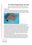
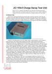
USER MANUAL:
JCI 155v4 Charge Decay Test Unit
UM155 - Issue 20: 3 October, 2000
A compact instrument for quick and direct measurement of the ability of materials to
dissipate static electricity
Note: This User Manual applies to JCI 155v4 Charge Decay Test Unit instruments made
and supplied with serial numbers over 0006****.
Contents:
1. INTRODUCTION
2. PRACTICAL DESIGN FEATURES
3. SPECIFICATION FEATURES
4. POWER SUPPLY AND BATTERY CHARGING ARRANGEMENTS
5. OUTPUT CONNECTIONS
6. SAFETY AND OPERATING PRECAUTIONS
7. INSTRUMENT SET UP FOR MEASUREMENTS
7.1 Introduction
7.2 'Beginners Guide'
7.3 Suggested Test Procedure
7.3.1 Equipment
7.3.2 Test samples
7.3.3 Test Environmental Conditions
7.3.4 Method
7.3.5 Test Report
7.4 Capacitance loading
7.5 Problems: What if... ?
8. INSTRUMENT SET UP AND CALIBRATION
8.1 Introduction
8.2 Basic access to circuits and mechanics
8.3 Access to mechanical features
8.4 Basic electrical checks on power supply circuit board
8.4 Checking, set up and calibration of fieldmeter
8.4.1 Introduction
8.4.2 Checking charge compensation
8.4.3 Checking sensitivity
8.4.4 Cleaning and resetting fieldmeter operation
8.4.5 Checking fieldmeter dynamic response
8.5 Check operation of high voltage power supply
8.6 Operational testing
8.7 Instrument calibration
9 REFERENCES
CE CONFORMANCE
John Chubb, proprietor of John Chubb Instrumentation of Unit 30, Lansdown Industrial Estate, Gloucester Road,
Cheltenham, GL5l 8PL, declares as designer and manufacturer, that the JCI 155 Charge Decay Test Unit conforms
to the requirements of the EC Directive on Electromagnetic Compatibility (EMC) 89/33/EEC to Standards EN
50081-1:1992 and EN 50082-1:1992. This instrument also conforms to the requirements of the Electrical Equipment
(Safety) Regulations 1994 (SDI. 1994/3260),
Signed for and on behalf of JCI:
John Chubb
October, 1998
Page - 2
USER MANUAL for JCI 155v4 Charge Decay Test Unit
The JCI 155 Charge Decay Test Unit is compact and easy to use instrument for measuring the
ability of materials to dissipate static electricity. If materials dissipate static quickly, and have
linkage to earth, then problems and risks with static will not arise.
1. INTRODUCTION
Many materials, in particular plastics, easily become electrostatically charged when rubbed
against other materials. Such 'triboelectric' charging causes problems in many areas of industry.
It can cause ignition of flammable gases and give shocks to personnel. It can make thin films and
light fabrics cling, attract airborne dust and debris, damage semiconductor devices and upset the
operation of microelectronic equipment.
The risks and problems arising from static electricity are best avoided by ensuring that static
charge can dissipate over and through the surfaces of materials and away to earth more quickly
than charge is likely to be generated. For normal manual handling and body actions this means
the charge decay time need to be below ½ second. Recent studies [1,16] suggest that decay
times may need to be nearer ¼ second.
The way to test the ability of materials to dissipate static electricity is to put some charge on the
material surface and see how quickly this charge disappears. In the JCI 155 a high voltage
corona discharge is used to deposit a patch of charge on the surface and a fast response
electrostatic fieldmeter is used to measure, without contact, the voltage generated by this charge
and how quickly this voltage falls as charge migrates away [2]. The method of assessing the
static charge dissipation capabilities of material used in the JCI 155 is included in a British
Standard [3] and an International Standard [4].
Corona charge deposition is the simplest way to simulate practical static changing events. It
allows control of initial surface voltage and charge polarity and is applicable for all types of
surfaces - whether uniform or with localised conducting features. Studies have shown that the
decay of corona charge matches well the practical situation of the decay of charge generated by
rubbing surfaces together [1,5,16]. A number of other studies have also been reported [6-13].
2. PRACTICAL DESIGN FEATURES
The JCI 155 Charge Decay Test Unit is a compact, self-contained unit which includes its own
high voltage supply for corona charging, a fast response 'field mill' fieldmeter for surface voltage
measurement and all the necessary controls, displays and data communication facilities for quick
and easy testing of materials under a wide variety of conditions.
Test Area: The JCI 155 rests directly on the test surface with a 45x54mm test aperture in the
instrument baseplate. Contact with the surface around the test area provides a return route for
outwardly migrating charge and high local capacitance to trap such charge.
Charging: The surface is charged by a high voltage corona discharge from points mounted as a
small conical cluster on the underside of a light plate which is moved between the fieldmeter
sensing aperture and the material surface under the instrument baseplate. A brief pulse
(e.g.20ms) of high voltage (up to about 10kV) causes corona discharges and deposits charge as a
patch in the middle of the exposed area of the material. Charge deposition time is short compared
to the minimum decay times which can usefully be measured. Pulse charge deposition ensures
that observations are little influenced by the position of the outer boundary. The moving plate
Page - 3
shields the fieldmeter from high voltage connections and corona ionisation so that reliable
measurements can be made down to low even surface voltages - for example 50-100V.
Fieldmeter: A proprietary design of fast response 'field mill' electrostatic fieldmeter is used to
provide sensitive and stable measurement of surface potential [14,15]. The response time to
surface voltage changes is below 10 ms and charge decay times can be measured to below 50
ms. The infinite input time constant means that reliable measurements can be made on materials
with even very long decay time constants - for example to well over 100,000 seconds.
Sample support: Measurements are normally made both with the material freely supported and
also resting against an earthed backing surface. These two arrangements represent the extremes
of practical constraints. The longer of the two decay times is used for assessment of the
suitability of the material. The JCI 166 Sample Support unit provides a simple arrangement for
such measurements. The JCI 176 provides facilities for measurement of the charge transferred to
the sample when testing with open backing [1].
Test conditions: Charge decay characteristics are susceptible to absorption of surface moisture
and so very likely to depend on humidity. It is desirable to carry out testing under defined, or at
least known, conditions of temperature and humidity. This can be achieved by carrying out
measurements in a controlled environment – as is provided, for example, in the JCI 191
Controlled Humidity Test Chamber, with at least 24 hours allowed for acclimatisation.
Test criteria: A simple acceptance test criterion is that the decay time (initial peak voltage to 1/e
(37%) of this), should be less than half a second. It is also useful to record how the rate of
charge decay varies during decay to see whether significant levels of charge are retained for long
times. Experience is that the form of charge decay curves does not usually depend on the level
of the initial peak voltage so such a ‘decay time’ is a useful simple number by which to rate
materials.
It is often observed that charge decay curves show a tendency to ‘plateau out’ after an initial
perhaps fairly rapid fall of surface voltage. In this situation it may be argued that a better
acceptance test criterion would be the time to 10% of the initial peak voltage – as this would
better ensure that residual surface voltages were low.
JCI 155 Operation: The JCI 155 will operate from its internal rechargeable batteries or directly
from the mains supply (100V-220V) when t5his is connected. The internal batteries provide
only about an hour of continuous operation.
Signal outputs and computer linkage: Analogue signal output connections enable observations
to be displayed and recorded on an oscilloscope or a paper chart recorder. An integral serial
communications interface enables decay curves to be transferred in real time to an IBM PC or
compatible microcomputer. JCI software (DECAY18E) provides automatic storage, display and
analysis of charge decay curve information. Opportunity is also provided to operate the JCI 155
under software control to preset test conditions of corona charging voltage and duration and to
make repetitive measurements.
Calibration: Instrument performance can be calibrated (BS 7506: Part 2: 1996 Annex 5) using
measurements whose accuracy is traceable to National Standards [3].
Page - 4
3. SPECIFICATION FEATURES
Controls:
- 3 position On/Off slide switch with operation by mains or integral
rechargeable batteries (in back plate).
- 3 position slide switch to 'Set for charging' and to 'Discharge'.
- 3 position high voltage on/off switch with middle position
providing 20 ms pulse of corona charging at instant of 'Discharge'
- high voltage level control potentiometer
- high voltage polarity changeover rotary switch
- 3 position slide switch to select display of surface voltage at:
- 'start of timing'
- 'present'
- 'end of timing'
- screwdriver zero adjustment for fieldmeter (2mm hole in front plate)
Displays:
- 8 digit liquid crystal display showing elapsed time in 0.001s units.
- 3½ digit liquid crystal display of corona voltage with polarity and LO
BATT indication.
- 4½ digit liquid crystal display of surface voltage selected as present
voltage, initial voltage at start of decay timing and voltage for end of
timing
Test area:
- 45x54 mm aperture in instrument Baseplate
Sample:
- the unit may be placed directly on a surface or area of sample
- the JCI 166 Sample Support Unit provides a simple support for open and
earthed backing tests
- the JCI 176 Charge Measuring Sample Support provides opportunity to
measure the corona charge received by the sample
- powders and liquids may be studied by placing these in an earthed cup
under the test aperture (e.g. JCI 170)
Fieldmeter:
- fast response 'field mill' fieldmeter measures surface voltage with
response time less than 10ms.
- 4½ digit liquid crystal digit with last digit equal to 1 volt of surface
potential.
- zero stability: within +10 V long term. Noise on liquid crystal display
within +1V, on analogue and serial data link outputs +5V.
Operating times:
- about 2 seconds to 'set for charging', 20 ms opening.
HV supply:
- internal feedback stabilised high voltage supply providing positive and
negative potentials to 8-10kV. A 10 Megohm personnel safety resistor is
used in the link to the corona discharge points.
Surface voltage:
- from about 50V to about 3kV, depending on charging conditions and rate
of charge dissipation on test surface
Measurement:
- from under 50ms to over 100,000 seconds
Operation:
- integral mains power supply with automatic selection between
Page - 5
240V/6VA 50Hz and 110V/6VA60Hz supplies. 250mA slow-blow fuse.
- automatic selection of operation between mains supplies or integral 100
mAh nickel hydride rechargeable batteries. Batteries provide about 1 hour
continuous operation
Battery charging: - the nickel metal hydride batteries are Smart charged whenever the
instrument is connected to the mains supplies but is not operating. Fast
recharging takes about an hour.
Connections:
- mains input via IEC connector
- combined Durable Dot and 4mm bayonet socket earth bonding
- signal outputs via 8w miniature DIN connector:
surface voltage (1V = 1000V surface volts)
corona voltage (1V = 4.0kV corona volts)
corona current (1V = 50µA)
serial data communications
Software:
- DECAY18E (or later versions) to transfer charge decay curve data into
an IBM PC or compatible micro operating MS DOS for analysis, display
and storage and for optional control of operation. JCI-Graph is also
available as an extra.
Dimensions:
- 173 x 216 x 67mm
Packaging:
- in carrying case with mains and signal output cables
4. POWER SUPPLY AND BATTERY CHARGING ARRANGEMENTS.
The switch to control operation of the Charge Decay Test Unit is at the lower right hand side of
the back plate of the instrument. If the instrument is connected to mains power supplies then
operation will be from the mains but if mains supplies are not available then operation is from
the internal rechargeable batteries. The upper of the two LEDs indicate the mains supply is
connected. The lower indicates fast recharging of the batteries. The switched mode power
supply covers supply voltages between 110V 60Hz and 230V 50Hz mains supplies. The
replaceable fuse in the backplate (by the IEC socket) should be a 250mA slow blow fuse.
The integral batteries are recharged by a Smart charging circuit that provides fast recharging
when needed and trickle charging for fully charged batteries. Fast charging is only provided
when the instrument is connected to the mains but is not operating. Full recharging will be
achieved in 1 - 1½ hours. The batteries will provide for up to about an hour of instrument
operation. If the batteries have been very fully discharged then initial charging is at a trickle
charging rate until the battery voltage has built up and charging can move into a fast charge
mode.
5. OUTPUT CONNECTIONS.
The 8 way miniature DIN connector on the backplate of the JCI 155 provides output of an
analogue signal of the fieldmeter observations and of the corona and current measurements and
also the RS 232 communication signals. The allocation of pins on the 8 way miniature DIN
socket and 9 way and 25 way D type connectors for serial data communications are as follows:
Page - 6
8w miniature DIN
1
black
2
white
3
TX
4
yellow
Surface volts 5
violet
Corona current 6
blue
RX
7
green
Corona volts 8
brown
RTS
earth
9w D type
7
1
25 way D type
4
7
3
2
1.0V = 1000V surface volts
1V = 50µA
2
5
3
2.5V = 10.0kV
cable screen
1
The serial data communication rate is set at 9600 baud by hardware links in the interface circuit.
The software, DECAY18E, accepts and handles data at this rate and achieves 400 12 bit
fieldmeter readings a second (2.5ms between readings).
6. SAFETY AND OPERATING PRECAUTIONS
Voltages up to 10kV can be applied to the corona discharge points. There is no risk of direct
shock or damage to an operator touching these points because there is a 10 Megohm high voltage
safety resistor in the supply line. However, contact with the corona discharge points when these
are energised should be avoided as a feeling of a shock may cause reactions which could lead to
indirect damage.
The JCI 155 should not be used in flammable atmospheres as it is not BASEEFA Certified.
Care must be taken during testing to avoid any material, surface or article projecting into the test
aperture. Such projections could be trapped by the brass strip 'air dam' on the moving plate and
trap the item and/or damage the instrument.
Care must be taken when testing powders, liquids or materials with loose surface fibres to avoid
these being swept into the test aperture as this may adversely affect instrument operation. In
particular, insulating powder particles or fibres on surfaces in and near the fieldmeter sensing
aperture are likely to cause appreciable zero offsets and zero drift. If it is desired to make
measurements on light powders easily dispersed into the air it will be wise to increase the
separation between the powder surface and the instrument baseplate. This will minimise the
influence on the powder surface of air movement induced by rapid movement of the air dam
when the moving plate is retracted. (Alternatively measurements may be made using a JCI 149).
7. INSTRUMENT SET UP FOR MEASUREMENTS
7.1 Introduction
Figure1 shows a top view of the JCI 155 instrument. Figures 2 and 3 show the underside of the
instrument with the plate carrying the corona discharge points advanced ready for charge
deposition and with the plate moved away to show the sensing aperture of the fieldmeter. The
operating principle of the JCI 155 is illustrated in Figure 4 and a typical fieldmeter response
signal as the moving plate moves away is shown in Figure 5.
7.2 'Beginners Guide'
•
Place instrument on a simple flat test surface - paper is a convenient initial test surface,
resting on a rigid flat surface.
•
Connect the JCI 155 to a mains supply with the IEC mains lead supplied. Switch on the
Page - 7
JCI 155 (Move the switch on the back plate of the instrument into the fully down position).
•
•
Place the instrument baseplate onto a conductive surface - for example a sheet of paper.
Check the fieldmeter zero with the switch on the right of the `Surface Voltage' LCD (top
right hand of instrument) into the middle position giving the 'present' surface voltage reading.
This should be close to 0000. If the reading is more than 1 or 2 digits positive or negative
use a small screwdriver to adjust the zero setting multiturn potentiometer through the 2.3 mm
adjustment hole in the front end plate of the instrument to give a reading close to 0000.
Select 'Operation control' as Instrument.
•
Select negative corona voltage (rotate the HV switch body with a small coin in the slot so
the spot is to the right hand side of the switch)
•
Move the corona control switch fully down to the `On Continuous' position and turn the
HV potentiometer clockwise to give maximum corona charging voltage - this will show as
about 10kV on the `Charging Voltage' LCD (top left side of instrument). Now move the
corona control switch to the middle, pulse, position.
•
Set for charging: Move the switch near bottom of the top cover into the forward `Set for
Charging' position. The motor advancing the plate carrying the corona discharge points will
be heard to run for about 2s and then stop. (Inspection of the underside of the instrument will
show the plate now in the forward position and the cluster of corona discharge points
visible).
•
Discharge: Move the lower switch down to the `Discharge' position. The plate will be
heard to flip back. The `Surface Voltage' LCD reading should show an excursion away from
zero and the counter in the middle of the instrument will start counting and then stop. (For
normal paper a decay time between 0.1 and 5s can be expected).
A basic fieldmeter response signal is shown in Figure 5. The fieldmeter signal rises to a peak in
about 20ms as the plate mounting the corona discharge points moves away and allows the
fieldmeter to observe the full surface potential created by the charged surface. A short time after
the initiation threshold is passed counting is started into a digital to analogue convertor (DAC) to
generate a rising ramp voltage. As this ramp voltage crosses the fieldmeter signal counting into
the DAC is stopped. This a) starts timing, and b) provides a value for the initial peak voltage.
The initial voltage is deliberately taken slightly after the signal maximum occurs to ensure it is
on the decaying part of the curve.
7.3 Suggested Test Procedure
The following procedure is suggested as likely to be suitable for general testing the ability of
materials and surfaces to dissipate electrostatic static charge. Alternative procedures may prove
to be more appropriate for particular materials.
Measurements based on decay times displayed directly on the JCI 155 are normally quite
satisfactory. The time from initial peak voltage to 1/e of this will be found to agree well with
values derived from software recording and analysis. Software recording and analysis is to be
preferred whenever this is practical because decay time values are based on a better analysis of
observations. Also, the actual decay curve data is available for inspection and reanalysis if need
Page - 8
be and the form of the decay curve can provide better insight into the character of the material
performance than can arise from a simple time from peak voltage to 1/e of this. (Software
system operation is described in an accompanying User Manual).
7.3.1 Equipment:
JCI 155 Charge Decay Test Unit
JCI 166 Sample Support or JCI 176 Charge Measuring Sample Support or JCI 170, for
powder samples
IBM PC or compatible microcomputer with CGA or better graphics running MSDOS
Software DECAY18E and RDUMP (for creating a simple summery of results)
Software JCI-Graph (for presentation of graphs and results within a Windows
operating environment)
Temperature and humidity measuring instrumentation (e.g. Casella whirling
hygrometer)
Humidity controlled test chamber (e.g. JCI 191)
7.3.2 Test Samples:
The charge decay characteristics of materials can easily be affected by moisture. It is therefore
important to test materials a) in well defined environmental conditions and after sufficient time
for the material to accommodate to these conditions, and b) in the 'as received' condition without
any handling, cleaning or removal of dust or dirt. The areas to be tested should not be contacted
by hand or by other surfaces and care should be taken not to blow or breath on the test surface.
The charge decay characteristics of powders and liquids may be tested by placing these in an
earthed cup under the instrument test aperture (e.g. a JCI 170). Care must be taken when testing
powders or materials with loose surface fibres to avoid these being swept into the test aperture as
this may adversely affect instrument operation. In particular, insulating powder particles or fibres
on surfaces in and near the fieldmeter sensing aperture are likely to cause appreciable zero
offsets and zero drift. If it is desired to make measurements on light powders easily dispersed
into the air it will be wise to increase the separation between the powder surface and the
instrument baseplate (e.g. using a JCI 172 Support Plate with a JCI 170 Powder Sample
Support). This will minimise the influence on the powder surface of air movement induced by
rapid movement of the air dam when the moving plate is retracted.
7.3.3 Test Environmental Conditions:
Because charge decay can be affected by the ambient temperature and humidity, particularly,
humidity, it is important:
a) for on-site measurements that the temperature and humidity be measured at the time of testing
and comment made of any likely changes in the 24 hours preceding testing
b) for laboratory testing that sample materials are exposed to constant standard conditions of
temperature and humidity for at least 24 hours before testing with measurements carried out in
these same environmental conditions. 'Standard conditions' are 23C 50%RH and 23C 12%RH or an alternative low level humidity considered appropriate to the minimum level likely to arise
in practical use. A JCI 191 Controlled Humidity Test Chamber is a convenient test situation.
7.3.4 Method:
The JCI 155 is placed on the JCI 166 Sample Support (or the JCI 176 Charge Measuring Sample
Support or JCI 170 Powder Sample Support) and linked with a double bayonet plug connection
lead. The mains cable to the JCI 155 is plugged in and the data cable linked from the 8 pin
miniature DIN connector to the serial data port of the microcomputer. The JCI 155 is switched
Page - 9
on and the zero setting checked, and if necessary adjusted, after a few minutes operation. The
JCI 155 is set for 'computer operation' and for negative corona operation.
Lift the JCI 155 off the sample support (or raise the top plate of the JCI 176) and place the test
area of the sample as a single layer on the JCI 166 Sample Support. Ensure the material is lying
flat. If rucks in the material enter the test aperture this could interfere with testing and possibly
jam instrument operation. Place the JCI 155 on to the material. Align the back edge of the JCI
155 with the back of the JCI 166 for 'open backing'. For 'earthed backing' tests align the test
aperture of the JCI 155 so the test aperture of the JCI 155 will be above the full metal area of the
JCI 166. The JCI 155 must remain steady and undisturbed on the test surface throughout the
whole of the measurement period. On uneven samples it may be appropriate to steady the JCI
155 with a hand.
The microcomputer is switched on and DECAY18 started via the icon provided at installation.
This ensures operation in true MSDOS mode (which is not achieved via the MSDOS window!)
The first menu may be used to set up and select an operating directory - but this need not be of
concern just to get started.
The second user menu is entered and the applicable values of temperature and humidity entered.
It is recommended that the options are taken a) to set ‘analysis period start voltage’ large (say
10000V) so analysis will start at whatever peak is achieved. Also, to set ‘analysis period end’ to
10% so this decay time is measured as well as the default time to 1/e..
It is useful to note that sample may become pre-charged by handling when placed ready for
testing. It is recommended that when samples are placed in position the moving plate is back so
the fieldmeter can respond to any charge on the sample surface and show these observations via
the surface voltage ‘at present time’. Two main options are available if there is appreciable precharge:
a) to wait until the pre-charge has dissipated. This means waiting for the initial surface voltage
to fall to say 10-50V, depending on the quality of observations aimed at.
b) to make a study on the decay of this pre-charge without adding any corona charge. This
means making a measurement with the corona voltage turned off or set for zero volts. It is to
be noted that the decay of such pre-charge may be rather slower than the decay of the local
patch of corona charge. It is none the less a useful observation.
It is not recommended that quality measurements are attempted by putting corona charge on to
an already well charged surface or material. It is also not recommended that pre-charge the
material is neutralised by any other means than waiting. Deposition of neutralising charge may
only give the appearance of neutrality.
There are two other possible artefacts are worth noting:
a) that if the air dam on the leading edge of the moving plate touches the sample surface then
tribocharging may occur. This may arise when testing light fabrics. The fabric surface
should be stretched flat but it may still rise by the induced air movement. This effect may be
checked by making measurements with no corona charging. It may be avoided by raising the
baseplate of the JCI 155 slightly off the sample.
b) That with some materials a very short (1-2ms) transient peak voltage is observed before the
real charge decay curve. This is usually positive. Occurrence of this transient will upset
operation of software timing. It is thought to be due to charge separation between the front
Page - 10
and back of the sample when this is flexed by the air movement of the air dam. The simple
way to avoid upsetting timing when operating with negative corona is to set the positive
threshold high (say 500V).
At the third software menu the sample description is entered - with notes on test conditions such
as open/earthed backing. The corona voltage and associated test conditions are also set at the
third menu. The default test conditions are checked to be 'corona voltage' 9000V and 'corona
duration' 0.02s. These will suffice for most materials.
From the third user menu press <return> on 'proceed'. The plate carrying the corona points will
be heard to be moved forwards and when fully forwards the computer screen will change to
show the axes for graphical display of charge decay observation. The moving plate will be heard
to flip back after a few seconds and the progress of charge decay will be shown on the screen.
When a suitable end point has been reached (either automatically or be pressing <esc>) the
computer will provide opportunity for numerical analysis and then graphical display of
observations.
Charge decay results are stored automatically and can be reviewed via the data directory in the
initial menu of DECAY18. If the graphical display is exited by pressing <return> (rather than
<esc>) the graph is stored as displayed. With older microcomputers this can be printed out
directly with the Screen Print command - or later using the program GPRINT.
A summary of the main features of a number of observations can be prepared later using the
program RDUMP. This creates a .CSV file that can be loaded into most Spreadsheet software
and enables the summary of results to be printed out or transferred into a report.
It is to be noted that the form of the charge decay curve, and the associated variation of decay
time constant during the decay, gives a much fuller picture of the behaviour of the material than
the simple 'decay time' value as the time from the initial peak surface voltage to 1/e or to 10% of
this. The two software programs GPRINT and RDUMP are MSDOS programs. Use of
GPRINT requires the operating system to be in true MSDOS and set into the GRAPHICS mode
appropriate for the printer connected. This may not be easy with more modern microcomputers.
JCI-Graph operating within a Windows syytem environment and allows up to 4 charge decay
graphs and associated variations of local decay time constants to be displayed and transferred
into other Windows applications – such as wordprocessing.
At least two measurements should be made at different positions on each test sample. If the
decay time is short then it will be useful in addition to retest the same position to show
consistency of results and lack of influence of the test on the sample surface. For this the surface
voltage should be allowed to fall to a low level (well below the expected end of timing level)
before retesting.
7.3.5 Test Report:
The following information shall be recorded:
a) date of measurements
b) description and identification of test material and location of test area
c) history of test sample (e.g. number of washes of fabrics)
d) temperature and relative humidity
e) test conditions of corona charging voltage, duration, polarity and whether open or earthed
backing
Page - 11
f) individual values of initial peak sample surface voltage and the time from peak voltage to 1/e
of this voltage. (For computer stored data the file reference of the test). Where measurements
are made of the charge received by the sample these values should be recorded and any
calculation made of 'capacitance loading'.
g) graph of the variation of surface voltage and charge decay time constant during charge decay
h) serial number of instrument used and date of most recent calibration
7.4 Capacitance Loading:
The influence of electrostatic charge on materials depends both on how long it is there and to the
associated surface voltage created. The quantity of charge per unit of initial peak surface voltage
is effectively a ‘capacitance’. If this capacitance is large then only low surface voltages will
arise from the quantities of charge likely to arise in practical tribocharging events. Many
materials, notably cleanroom garment fabrics including conductive threads, show high values of
‘capacitance’ so although their charge decay times may be long it may be they present little risk
of causing problems.
Measurements of the quantity of corona charge transferred to a sample using a JCI 176 Charge
Measuring Sample Support. The ‘initial peak voltage’ as measured by the JCI 155 is related to a
voltage on a conducting plane across the whole test aperture area. When corona charge is
deposited the area of charge is much smaller than this area so the local voltage will be much
higher. Rather than express ‘capacitance’ in terms of a guessed area of charge it is more
practical to assess materials in terms of their ‘capacitance loading’ [1,16]. This is the
‘capacitance’ value observed for the test material divided by the ‘capacitance’ value observed for
a very thin dielectric layer, such as cling film.
The corona charge deposited on the sample is measured, with a JCI 176, as a combination of the
conduction and induction charge values. By using a simple dissipative sample material, such as
paper or cling film, it is observed that the initial charge signal is just an induction signal, Qi, and
that as this moves out it becomes just a conduction signal Qc. By finding the factor, f, that
matches the fall of induction signal to the rise of the conduction signal the total charge Qtot can
be calculated as
Qtot = Qc + f * QI
The geometry of the JCI 176 was designed to give f ~ 2. Experience shows values close to 1.8.
When the JCI 176 is used with samples and surfaces that have very fast charge decay times it
needs to be recognised that the ultimate performance may be limited by effects due to residual
air ionisation. The air dam on the moving plate very effectively removes residual air ionisation
when JCI 155 instruments are used with the baseplate resting directly on the sample surface.
When used with the JCI 176 there is opportunity for ionised air to leak back to the region in front
of the fieldmeter. Typically this will give apparent initial peak surface voltages of 10-20V for
maximum charge transfers around 2000nC, and show decay times around 100ms. If charge
decay performances of such levels are observed, it will be wise to check instrument operation
with a fully conducting surface mounted in the sample position of the JCI 176.
7.5 Problems: What if...?
7.5.1 If the LCDs do not show any numbers when the power is switched on:
- with battery operation it may be the batteries are flat and need to be recharged. Try mains
operation.
- if mains operation has been selected check if the mains power supply is really on. This is
shown by the mains led. If the instrument only operates at all from batteries then the mains fuse
Page - 12
has probably blown and should be checked and replaced
7.5.2 If the surface voltage `at present time' fluctuates more than +5V, or if the zero setting has
changed appreciably during use or is drifting, the sensing region of the fieldmeter may need
cleaning. This needs to be carried out with some care. The fieldmeter sensing section can be
taken out through the test aperture as described in section 8.4.4.
7.5.3 If the reading of the high voltage LCD fluctuates appreciably with the HV switched to
continuous operation there may he a problem with the high voltage module. This may cause
premature triggering of the timing circuits or the software or may limit maximum high voltage
levels. Operation with brief corona (20ms) charge deposition is more likely to continue to be
satisfactory. Contact JCI and expect to need to return the instrument for servicing.
7.5.4 If the `elapsed time' LCD does not start to count or shows a time of only a few ms (below
20) then the timing circuits did not trigger properly. This may be because vertical flexing of the
sample has created some surface charge by internal tribo of piezoelectric effects. Although this
charge is able to neutralise itself very quickly it may give an excursion of the fieldmeter
observations which trigger and upset operation of the timing circuits.
7.5.5. Decay timing will not start on the instrument unless the test surface voltage excursion is
greater than about 50V so if timing does not start it may be useful to try a higher corona voltage
or to change from a 20ms to charging for a few seconds. Negative corona produces stronger
charging. It is useful to check basic instrument operation with a material which normally will
give satisfactory operation - for example paper. With software monitoring try reducing the
'threshold voltage' for the polarity of charging - 20V is probably a sensible minimum. If timing
still does not start it is probable that the materials tested has such a fast charge decay that it is not
feasible to create a sufficient surface voltage to allow measurements to be made. This point
should be recorded in the Test Report.
7.5.6 If the charge decay time is very short, 0.1s or less, and the initial peak voltage is very low it
will sometimes be observed that the timer counter shows a time around 2.4 seconds. This is an
artefact – of unknown origin! When handling materials which give short decay times and very
low initial peak voltages it is always wise to make observations and measurements using
software so the real form of the decay curve and the influence of signal noise can be
appreciated..
7.5.7. If the movement of the plate carrying the corona discharge points jams, then check
whether this was due to material getting into the test aperture. If so carefully remove the
obstruction - and if necessary straighten the brass 'air dam' if this was bent. If the mechanism
itself has jammed with the plate part way back then try pushing the plate forwards by finger
pressure near the base of the brass sheet 'air dam' and check if the drive motor runs freely with
the plate held forwards. If the plate does not move easily in its guide slots it may be useful to try
wiping these with a piece of link free tissue or cloth with a little light solvent. Do NOT lubricate
the slides with oil. If the plate is jammed fully forwards and the motor runs freely then carefully
try to prize the 'air dam' away from the front edge of the aperture - but take care as the plate may
fly back fast. If the motor does not run freely it maybe that there is some obstruction in the gear
train. It may be that this can be spotted by removing the back plate of the instrument and very
carefully incrementing the gear train by hand - if not the instrument must be returned to JCI for
servicing.
Page - 13
7.5.8 If the motor driving the plate carrying the corona points runs on continuously or if the plate
flips back as soon as it is fully advanced and before the swtch is moved to the ‘Discharge’
position then the angular setting of the cam sensor PCB may need adjusting. This can be
accessed directly when the back plate is removed. The small cam sensor PCB is a small circuit
board in the middle close behind the back plate - and down near the instrument baseplate. This is
secured by two M2 screws on either side of the PCB. If these are carefully loosened then the
PCB can be slid slightly to the right (e.g. 1-2mm) to stop the cam a little earlier. The two M2
screws are then retightened and, after checking operation, the back plate is replaced. When
replacing the backplate make sure that the leads will not be trapped and will not lie down in the
track of the cam or main gear. Make sure the two LEDs at the back of the PCB on the right hand
side (just above the switch) go into their holes in the backplate.
8. INSTRUMENT SET UP AND CALIBRATION
8.1 Introduction
The JCI 155 Charge Decay Test Unit is carefully set up and calibrated during manufacture. No
internal adjustments should be attempted unless suitable instruments and facilities are available
to also check calibration. In general it will be best to return an instrument to JCI for servicing if
operation becomes unsatisfactory. The notes in Section 7.4 provided a basic appreciation of
possible problems and their likely cause and remedy. The following notes apply to JCI 155
instruments made from January 1998.
8.2 Basic access to circuits and mechanics.
The following steps are needed to gain access to the inside of the Charge Decay Test Unit.
Dismantling should take place on a clean flat surface with suitable receptacles to store screws
and parts removed. Only proceed as far as needed for the access required.
- remove the two M3x8 screws in the back plate, carefully ease out the plate from the side
extrusions and fold down with its internal wiring connections
- remove the two M3x8 screws in the front plate and then slide the two side extrusions off the
compression pins on the front plate.
- carefully remove (e.g. using a finger nail) the cap from the high voltage potentiometer setting
knob, then holding the knob loosen the internal screw and lift off the knob
- carefully undo and remove the nut securing the body of the high voltage potentiometer to the
top cover. The top cover may now be removed by lifting off from the back end to allow the
cover to disengage from the slot across the front plate. The main signal processing circuit board
is now exposed. The power supply circuit card is on the right hand side of the instrument and the
high voltage supply board is on the left.
The physical arrangement of components, test points and adjustment potentiometers for the main
signal processing and fieldmeter circuit beard, for the power supply and for the high voltage
supply circuit board are shown in Figures 6, 7 and 8. The identities of the various leads of the
inter-board flexible connections are also listed in these figures. While there are a number of
components on the reverse (inner) side of the power supply PCB most diagnostic work can be
carried out without further disassembling the instrument. The instrument can be operated quite
satisfactorily with the covers off and the circuits undisturbed at this stage. The cover over the
fieldmeter section usefully reduces interference noise, and so should be left in place for
instrument testing.
8.3 Access to mechanical features
The mechanical system is accessed from the disassembled state above as follows:
Page - 14
Remove the two M3 screws securing the folded aluminium shield over the fieldmeter region and
remove the two phosphor bronze spring trapped by these screws. These springs make earthing
contact with the underside of the top cover. Lift off the fieldmeter shield. Unscrew the two
hexagonal pillars securing the main PCB to the mechanical structure. Disconnect the flexible
connection strips from the main PCB to the power supply PCB and to the HV supply PCB.
Gently lift up the main PCB and disconnect the lead to the mechanism motor drive and the lead
to the microswitch below the PCB. Lift the PCB clear. Lift out the power supply PCB. Unscrew
the 2 M3x20 screws securing the HV module and lift that out. Remove the 3 M2 screws
securing the shield over the top of the mechanism structure. If necessary the mechanism can
now be separated from the baseplate by unscrewing the 3 M3x8 screws securing it to the
baseplate.
Reassembly is the reverse of the above sequence.
8.4 Basic electrical checks on power supply circuit board.
The basic layout of components on the Power Supply circuit board is shown in Figure 7.
With the instrument case opened as 8.3 above, or with the power supply circuit card supported
on an insulating surface and the mains supply connected to the Molex connector on the back of
the board near the transformer: The same voltages as below should be observed with 230V or
115V mains supplies or when operating from fully charged batteries.
- connect to the mains supply and switch ON. Check that the middle led lights with mains
switch on.
- check at PLl/2 relative to PLI/l,3,5,7,or 9 as 0V, that the rail voltage of the supply with mains
operation is about +15V and is free from noise and ripple. (Take care not to short rail to rail).
- check at PLl/4 relative to PLI/l,3,5,7,or 9 as 0V, that the rail voltage of the supply with mains
or battery operation is +12V and is free from noise and ripple. (Take care not to short rail to rail).
- check at PLl/6 relative to PLI/l,3,5,7,or 9 as 0V, that the rail voltage of the supply with mains
or battery operation is +8.2V and is free from noise and ripple. (Take care not to short rail to
rail).
- check at PLl/8 and at /10 relative to PLI/l,3,5,7,or 9 as 0V, that the rail voltage of the supply
with mains or battery operation are +5V and free from noise and ripple. (Take care not to short
rail to rail).
-check at PLl/12 relative to PLI/l,3,5,7,or 9 as 0V, that the rail voltage of the supply with mains
or battery operation is -5V and is free from noise and ripple. (Take care not to short rail to rail).
- check that the upper led comes on to indicate `fast charging if the mains is connected and the
ON/OFF switch is moved to the OFF position. The current for fast and trickle charging can be
measured from the voltage across the 2R7 charging resistor (R22) - 270mV for fast charge and
about 13mV for trickle charging..
8.4 Checking, set up and calibration of fieldmeter
8.4.1 Introduction
There are 3 activities which may be needed with the fieldmeter:
- checking and possibly adjusting sensitivity
- checking and possibly adjusting charge compensation
- disassembly, cleaning and resetting fieldmeter operation
The fieldmeter used in the JCI 155 is basically two 'field mill' fieldmeter units mounted back to
back so there is no need to have the chopping rotor earthed. This proprietary approach has been
Page - 15
described in published papers [14,15]. These should be consulted to gain understanding of
instrument principles and operation.
Access to the potentiometers to set charge compensation and sensitivity of the fieldmeter can be
gained through the test aperture. Alternatively, access can be gained with the front plate of the
JCI 155 removed . If the instrument has been taken apart, as 8.2 above, it is recommended that
charge compensation and sensitivity of the fieldmeter are checked and adjusted with the
fieldmeter shield in place.
8.4.2 Checking charge compensation
The zero setting of the fieldmeter should be independent of the presence of charge on the
rotating chopper. The procedure to check and set the compensation is as follows:
- switch off the JCI 155 and allow the rotating chopper to come to a stop.
- earth the chopper to the front aperture of the fieldmeter using a clean dry small metal rod
- switch on the JCI 155 and note the zero reading after a few moments operation
- switch off the JCI 155 and allow the rotating chopper to come to a stop.
- apply a voltage to the chopper blades. (A 9V PP3 battery is a convenient source with one
terminal earthed and a lead with just a little contact length beyond the insulation used to make
contact with the rotor blades)
- switch on the JCI 155 and note the reading
- if this differs from the previous 'earthed rotor' value then adjust the rightmost (leftmost through
the test aperture) potentiometer (RV400) to make the reading the same
- switch off the JCI 155 and allow the rotating chopper to come to a stop and repeat the above
'earthed' and 'charged' rotor sequence until the zero reading remains the same.
8.4.3 Checking sensitivity
The fieldmeter is carefully set up and calibrated during manufacture. No adjustments should be
attempted unless suitable instruments and facilities are available. The following notes describe
appropriate set up and calibration procedures.
The fieldmeter is most simply checked and calibrated in position in the Charge Decay Test Unit
in terms of a uniform potential across a surface covering the whole area of the test aperture and
just below the plane of the test area aperture. While setting the sensitivity it is necessary to have
the front end plate (or an equivalent metal surface) in position. The sensitivity is best set with a
voltage of 1000V applied to this plate. Adjustment of sensitivity is by the leftmost potentiometer
(RV401) of the 4 pots along the top edge of the main PCB (rigthmost as viewed through the test
aperture).
8.4.4 Cleaning and resetting fieldmeter operation
Noisy and variable fieldmeter zero signals indicate that the inside of the sensing region is
contaminated, for example by insulating particles or fibres. In this situation it is necessary to
dismantle the sensing system, clean it, reassemble and reset operation - including setting charge
compensation and sensitivity as above.
The fieldmeter sensing section can be taken out through the test aperture by unscrewing the 3
M2x16 screws around the edge of the gold plated body outside the sectored sensing aperture. It
is important NOT to disturb the 5 M1.6 screws in a ring nearer the sensing aperture. With the 3
M2 screws removed the cylindrical brass body can be carefully pulled out - with care to pull it
straight down and not at an angle. Removal of the 3 M1.6 screws around the edge of the PCB
holding the motor will allow the motor and rotor assembly to be removed from the cylindrical
Page - 16
body. The chopper assembly and the inside of the cylindrical housing can now be inspected in
good side illumination for the presence of any dust, contamination or fibres and this removed. It
may also be useful to sluice out the sensing region and the rotor assembly with a brief spray of
aerosol solvent. The sensor assembly should be reassembled and care taken to ensure the
original angular alignment is maintained of the PCB to the housing. When the sensor assembly
is remounted through the JCI 155 test aperture care is needed to ensure that both sets of 3
contacts align correctly and mate with the corresponding sockets mounted on the main circuit
board within the body of the JCI 155. Secure the fieldmeter sensor unit with the 3 M2x16
screws. Switch on the instrument and check a) the fieldmeter motor rotates, and b) the
fieldmeter is sensitive to nearby charge. Before using the JCI 155 the charge compensation
should be checked as in 8.4.2. It may also be useful to check the sensitivity of the fieldmeter, if
suitable facilities are available, as in 8.4.3. If the problem persists it may well be best to return
the instrument to JCI.
If checking charge compensation showed a significant error it will be wise to check if the rotor is
loose on the motor shaft by lightly pulling it. If it is loose then it is necessary to pull it as clear
of the shaft as is easy, to put a small drop of anaerobic glue on to the shaft and then carefully
slide the rotor back until the front chopper is 0.7mm from the front of the sensing surface.
To set-up basic fieldmeter operation when the main PCB has been accessed:
- connect an oscilloscope probe lead to TP12
- apply a voltage (for example l000V) to the calibration test plate and observe the waveform at
TP12
- check the signals at TP12 are a set of well balanced negative half sine waves for a positive
potential on the test plate.
Now check charge compensation and sensitivity as 8.4.2 and 8.4.3 above. With the shield in
place over the top of the fieldmeter circuitry the noise on the fieldmeter signal should be less
than +5V (+5mV p-p as viewed by an oscilloscope) and as observed by software recording of the
first 3s of charge decay curves.
8.4.5 Checking fieldmeter dynamic response
The dynamic response of the fieldmeter may be checked if the plate used for calibration above is
energised from a square wave signal generator and the fieldmeter output observed on an
oscilloscope. If the voltage swing of the signal generator is rather modest, say only 20V, then it
will be better to apply this to a disc or small metal plate introduced through the test aperture so as
to lie close to the sensing aperture of the fieldmeter so there is a reasonable signal to observe.
The response time of the fieldmeter should be below 10ms.
8.5 Check operation of high voltage power supply
- connect oscilloscope probe lead to junction of diode D8 linking to transformer and set probe to
x10 on 5V range
- move high voltage control switch (SW5 on main board) down to 'on' position and turn
potentiometer slowly towards maximum (clockwise) observing signal waveform on scope. The
waveform should be a train of full wave oscillations at about 200kHz each preceded by about a
15us period of slightly negative voltage. The repetition rate of the pulses should be close to
1kHz
- check potentiometer can be turned fully clockwise without any breakdown showing on the
signal waveform
-adjust RV2 (varying the time of the initial current flow) for maximum peak to peak signal
Page - 17
amplitude (about 120V pk to pk)
-move HV control switch to middle 'pulse' position; move plate movement control switch to
middle position; set the oscilloscope timebase to 5ms/div and triggering from the presence of the
HV energisation pulses; check that as the plate movement control switch is moved to the
'discharge' position that the train of HV pulses lasts close to 20ms; adjust RV1 to achieve 20ms.
- with moving plate in fully forward position link input connection of JCI 148 Electrostatic
Voltmeter to corona discharge points and check the voltage corresponds to that shown on LCD3`
8.6 Operational testing
Operational testing is best carried out with the JCI 155 mounted on a calibration unit with
defined value resistors and capacitors to earth from the test plate across the test aperture. It may
also be carried out using a simple dissipative test surface such as paper.
Use a double beam oscilloscope (with a 10 or 20 ms/cm timebase) to examine the waveform of
the fieldmeter signal and the response of the digital to analogue converter generating the 'start
voltage' signal (IC03/7). The time-base is best triggered near the start of the rise of the fieldmeter
signal. The two traces should be arranged to have the same zero deflection setting (so they
overlap) and have the same sensitivity (for example 50 mV).
When the instrument is operated a fieldmeter signal is expected as indicated in Figure 5. The
signal at IC03/7 is the DAC ramp signal and this should rise to intercept the fieldmeter signal a
short time after the fieldmeter signal peak - as indicated in Figure 5. The DAC level signal
should correspond to the fieldmeter signal at the intercept point. This should apply with both
corona polarities and with both fast and very slow charge decay rate surfaces.
The performance of the 'end of timing' comparator (IC32) is most easily checked by comparing
the decay times measured at positive and negative charging polarities with low charging voltages
and carefully adjusting RV8.
8.7 Instrument Calibration.
Instrument calibration is carried out to the procedure described in the new British Standard BS
7506: Part 2: 1996 Annex A5 [3].
Page - 18
9. REFERENCES
[1] J. N. Chubb “Measurement of tribo and corona charging features of materials for assessment
of risks from static electricity” IEEE-IAS Meeting, Phoenix, Arizona, Oct 1999 To be published
in Trans IEEE Ind Appl.
[2] J. N. Chubb "Instrumentation and standards for testing static control materials" IEEE Trans.
Ind. Appl. 26 (6) Nov/Dec 1990, p 1182.
[3] British Standard 'Methods for measurements in electrostatics' BS 7506: Part 2: 1996
[4] IEC 61340-5-1: 1998 “Electrostatics – Part 5-1: Protection of electronic devices from
electrostatic phenomena – General requirements” (Technical Report) International
Electrotechnical Commission
[5] J. N. Chubb "Dependence of charge decay characteristics on charging parameters"
Proceedings of 'Electrostatics 1995' Conference, University of York, April 3-5, 1995 Inst Phys
Confr Series 143 p103
[6] J. N. Chubb, P. Malinverni "Experimental comparison of methods of charge decay
measurements for a variety of materials" EOS/ESD Symposium, Dallas, 1992
[7] J. N. Chubb "Testing how well materials dissipate static electricity" British Plastics and
Rubber, May 1995 p8 MCM Publishing Ltd
[8] J. N. Chubb "Avoiding risks from static electricity" Evaluation Engineering, Sept 1995 p 57
[9] J. N. Chubb "Corona charging of practical materials for charge decay measurements" J.
Electrostatics 37 (1&2) 1996 p53
[10] J. N. Chubb "Reappraising static materials" Cleanroom Technology Winter 95/96 p4
[11] J. N. Chubb "Static: A material problem" Converting Today, May 1996 p21
[12] J. N. Chubb "Instrumentation to assess the static charge dissipation capabilities of
materials" 13th Int Symp Contamination Control, The Hague 16-20 Sept, 1996
[13] J. N. Chubb "Instrumentation and measurements to assess electrostatic conditions and
risks in cleanroom situations" Cleanroom Technology Expo Confr. Frankfurt 5/6 May 1998
[14] J. N. Chubb "Two new designs of 'field mill' type fieldmeters not requiring earthing of
rotating chopper" IEEE Trans. Ind. Appl. 26 (6) Nov/Dec 1990, p 1178.
[15] J. N. Chubb “Experience with electrostatic fieldmeters with no earthing of the rotating
chopper” ‘Electrostatics 1999 Inst Phys Confr Series 163 p443
[16] J. N. Chubb “New approaches for testing materials” Proceedings ESA Annual meeting,
Brock Univesity, Niagara Falls, June 18-21, 2000
Page - 19