1
User Manual of the RODIN Platform
July 2007
Version 1.4
User Manual of the RODIN Platform
Contents
1
2
Project
1
1.1
Project Constituents and Relationships . . . . . . . . . . . . . . . . . . . . . . . . . . .
1
1.2
The Project Explorer . . . . . . . . . . . . . . . . . . . . . . . . . . . . . . . . . . . .
1
1.3
Creating a Project . . . . . . . . . . . . . . . . . . . . . . . . . . . . . . . . . . . . . .
3
1.4
Removing a Project . . . . . . . . . . . . . . . . . . . . . . . . . . . . . . . . . . . . .
3
1.5
Exporting a Project . . . . . . . . . . . . . . . . . . . . . . . . . . . . . . . . . . . . .
4
1.6
Importing a Project . . . . . . . . . . . . . . . . . . . . . . . . . . . . . . . . . . . . .
4
1.7
Changing the Name of a Project . . . . . . . . . . . . . . . . . . . . . . . . . . . . . .
5
1.8
Creating a Component . . . . . . . . . . . . . . . . . . . . . . . . . . . . . . . . . . .
5
1.9
Removing a Component . . . . . . . . . . . . . . . . . . . . . . . . . . . . . . . . . .
6
Anatomy of a Context
6
2.1
Carrier Sets . . . . . . . . . . . . . . . . . . . . . . . . . . . . . . . . . . . . . . . . .
7
2.1.1
Carrier Sets Creation Wizard. . . . . . . . . . . . . . . . . . . . . . . . . . . .
7
2.1.2
Direct Editing of Carrier Sets. . . . . . . . . . . . . . . . . . . . . . . . . . . .
7
2.2
Enumerated Sets . . . . . . . . . . . . . . . . . . . . . . . . . . . . . . . . . . . . . .
8
2.3
Constants . . . . . . . . . . . . . . . . . . . . . . . . . . . . . . . . . . . . . . . . . .
9
2.3.1
Constants Creation Wizard. . . . . . . . . . . . . . . . . . . . . . . . . . . . .
9
2.3.2
Direct Editing of Constants. . . . . . . . . . . . . . . . . . . . . . . . . . . . .
10
Axioms . . . . . . . . . . . . . . . . . . . . . . . . . . . . . . . . . . . . . . . . . . .
11
2.4.1
Axioms Creation Wizard. . . . . . . . . . . . . . . . . . . . . . . . . . . . . .
11
2.4.2
Direct Editing of Axioms. . . . . . . . . . . . . . . . . . . . . . . . . . . . . .
11
Theorems . . . . . . . . . . . . . . . . . . . . . . . . . . . . . . . . . . . . . . . . . .
12
2.5.1
Theorems Creation Wizard. . . . . . . . . . . . . . . . . . . . . . . . . . . . .
12
2.5.2
Direct Editing of Theorems. . . . . . . . . . . . . . . . . . . . . . . . . . . . .
13
2.6
Adding Comments . . . . . . . . . . . . . . . . . . . . . . . . . . . . . . . . . . . . .
13
2.7
Dependencies . . . . . . . . . . . . . . . . . . . . . . . . . . . . . . . . . . . . . . . .
14
2.8
Pretty Print . . . . . . . . . . . . . . . . . . . . . . . . . . . . . . . . . . . . . . . . .
15
2.4
2.5
i
3
Anatomy of a Machine
16
3.1
Dependencies . . . . . . . . . . . . . . . . . . . . . . . . . . . . . . . . . . . . . . . .
16
3.2
Variables . . . . . . . . . . . . . . . . . . . . . . . . . . . . . . . . . . . . . . . . . .
16
3.2.1
Variables Creation Wizard. . . . . . . . . . . . . . . . . . . . . . . . . . . . . .
16
3.2.2
Direct Editing of Variables. . . . . . . . . . . . . . . . . . . . . . . . . . . . . .
17
Invariants . . . . . . . . . . . . . . . . . . . . . . . . . . . . . . . . . . . . . . . . . .
18
3.3.1
Invariants Creation Wizard. . . . . . . . . . . . . . . . . . . . . . . . . . . . .
18
3.3.2
Direct Editing of Invariants. . . . . . . . . . . . . . . . . . . . . . . . . . . . .
18
Theorems . . . . . . . . . . . . . . . . . . . . . . . . . . . . . . . . . . . . . . . . . .
19
3.4.1
Theorems Creation Wizard. . . . . . . . . . . . . . . . . . . . . . . . . . . . .
19
3.4.2
Direct Editing of Theorems. . . . . . . . . . . . . . . . . . . . . . . . . . . . .
19
Events . . . . . . . . . . . . . . . . . . . . . . . . . . . . . . . . . . . . . . . . . . . .
20
3.5.1
Events Creation Wizard. . . . . . . . . . . . . . . . . . . . . . . . . . . . . . .
20
3.5.2
Direct Editing of Events. . . . . . . . . . . . . . . . . . . . . . . . . . . . . . .
21
3.6
Adding Comments . . . . . . . . . . . . . . . . . . . . . . . . . . . . . . . . . . . . .
22
3.7
Pretty Print . . . . . . . . . . . . . . . . . . . . . . . . . . . . . . . . . . . . . . . . .
22
3.8
Dependencies: Refining a Machine . . . . . . . . . . . . . . . . . . . . . . . . . . . . .
23
3.9
Adding more Dependencies . . . . . . . . . . . . . . . . . . . . . . . . . . . . . . . . .
23
3.9.1
Abstract Event . . . . . . . . . . . . . . . . . . . . . . . . . . . . . . . . . . .
23
3.9.2
Splitting an Event . . . . . . . . . . . . . . . . . . . . . . . . . . . . . . . . . .
24
3.9.3
Merging Events . . . . . . . . . . . . . . . . . . . . . . . . . . . . . . . . . . .
24
3.9.4
Witnesses . . . . . . . . . . . . . . . . . . . . . . . . . . . . . . . . . . . . . .
25
3.9.5
Variant . . . . . . . . . . . . . . . . . . . . . . . . . . . . . . . . . . . . . . .
26
3.3
3.4
3.5
4
Saving a Context or a Machine
27
4.1
Automatic Tool Invocations . . . . . . . . . . . . . . . . . . . . . . . . . . . . . . . . .
27
4.2
Errors. The Problems Window . . . . . . . . . . . . . . . . . . . . . . . . . . . . . . .
27
5
The Proof Obligation Explorer
28
6
The Proving Perspective
31
6.1
Loading a Proof . . . . . . . . . . . . . . . . . . . . . . . . . . . . . . . . . . . . . . .
31
6.2
The Proof Tree . . . . . . . . . . . . . . . . . . . . . . . . . . . . . . . . . . . . . . .
32
6.2.1
Description of the Proof Tree . . . . . . . . . . . . . . . . . . . . . . . . . . . .
32
6.2.2
Decoration . . . . . . . . . . . . . . . . . . . . . . . . . . . . . . . . . . . . .
33
ii
6.2.3
Navigation within the Proof Tree . . . . . . . . . . . . . . . . . . . . . . . . . .
33
6.2.4
Hiding . . . . . . . . . . . . . . . . . . . . . . . . . . . . . . . . . . . . . . .
33
6.2.5
Pruning . . . . . . . . . . . . . . . . . . . . . . . . . . . . . . . . . . . . . . .
33
6.2.6
Copy/Paste . . . . . . . . . . . . . . . . . . . . . . . . . . . . . . . . . . . . .
33
6.3
Goal and Selected Hypotheses . . . . . . . . . . . . . . . . . . . . . . . . . . . . . . .
34
6.4
The Proof Control Window . . . . . . . . . . . . . . . . . . . . . . . . . . . . . . . . .
35
6.5
The Smiley . . . . . . . . . . . . . . . . . . . . . . . . . . . . . . . . . . . . . . . . .
37
6.6
The Operator ”Buttons” . . . . . . . . . . . . . . . . . . . . . . . . . . . . . . . . . . .
37
6.7
The Search Hypotheses Window . . . . . . . . . . . . . . . . . . . . . . . . . . . . . .
37
6.8
The Automatic Post-tactic . . . . . . . . . . . . . . . . . . . . . . . . . . . . . . . . .
37
6.8.1
Rewrite rules . . . . . . . . . . . . . . . . . . . . . . . . . . . . . . . . . . . .
38
6.8.2
Automatic inference rules . . . . . . . . . . . . . . . . . . . . . . . . . . . . .
42
Interactive Tactics . . . . . . . . . . . . . . . . . . . . . . . . . . . . . . . . . . . . . .
44
6.9.1
Interactive Rewriting Rules . . . . . . . . . . . . . . . . . . . . . . . . . . . . .
44
6.9.2
Interactive Inference rules . . . . . . . . . . . . . . . . . . . . . . . . . . . . .
49
6.9
7
8
Syntax of the Mathematical Language
50
7.1
Syntax for Predicates . . . . . . . . . . . . . . . . . . . . . . . . . . . . . . . . . . . .
51
7.2
Syntax for Expressions . . . . . . . . . . . . . . . . . . . . . . . . . . . . . . . . . . .
52
Appendix: ASCII Representations of the Mathematical Symbols
53
8.1
Atomic Symbols . . . . . . . . . . . . . . . . . . . . . . . . . . . . . . . . . . . . . .
53
8.2
Unary Operators . . . . . . . . . . . . . . . . . . . . . . . . . . . . . . . . . . . . . . .
54
8.3
Assignment Operators . . . . . . . . . . . . . . . . . . . . . . . . . . . . . . . . . . .
54
8.4
Binary Operators . . . . . . . . . . . . . . . . . . . . . . . . . . . . . . . . . . . . . .
55
8.5
Quantifiers . . . . . . . . . . . . . . . . . . . . . . . . . . . . . . . . . . . . . . . . . .
56
8.6
Bracketing . . . . . . . . . . . . . . . . . . . . . . . . . . . . . . . . . . . . . . . . . .
56
iii
The reader of this Manual is supposed to have a basic acquaintance with Eclipse.
1
1.1
Project
Project Constituents and Relationships
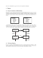
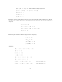
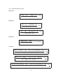
The primary concept in doing formal developments with the Rodin Platform is that of a project. A project
contains the complete mathematical development of a Discrete Transition System. It is made of several
components of two kinds: machines and contexts. Machines contain the variables, invariants, theorems,
and events of a project, whereas contexts contain the carrier sets, constants, axioms, and theorems of a
project:
Context
Machine
carrier sets
constants
axioms
theorems
variables
invariants
theorems
events
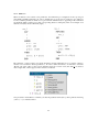
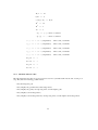
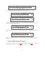
We remind the reader of the various relationships existing between machines and contexts. This is
illustrated in the following figure. A machine can be ”refined” by another one, and a context can be
”extended” by another one (no cycles are allowed in both these relationships). Moreover, a machine can
”see” one or several contexts. A typical example of machine and context relationship is shown below:
sees
Context
Machine
extends
refines
sees
Context
Machine
refines
1.2
extends
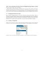
The Project Explorer
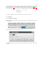
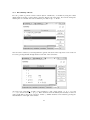
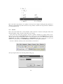
Projects are reachable in the RODIN platform by means of a window called the ”Project Explorer”. This
window is usually situated on the left hand side of the screen (but, in Eclipse, the place of such windows
can be changed very easily). Next is a screen shot showing a ”Project Explorer” window:
1
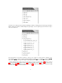
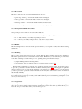
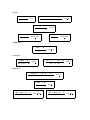
As can be seen on this screen shot, the Project Explorer window contains the list of current project names.
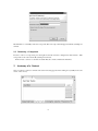
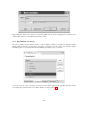
Next to each project name is a little triangle. By pressing it, one can expand a project and see its components as shown below.
We expanded the project named ”celebrity”. This project contains 2 contexts named ”celebrity ctx 0”
and ”celebrity ctx 1”. It also contains 4 machines named ”celebrity 0” to ”celebrity 3”. The icons ((c) or
(m)) situated next to the components help recognizing their kind (context or machine respectively)
In the remaining parts of this section we are going to see how to create (section 1.3), remove (section
1.4), export (section 1.5), import (section 1.6), change the name (section 1.7) of a project, create a component (section 1.8), and remove a component (section 1.9). In the next two sections (2 and 3) we shall
see how to manage contexts and machines.
2
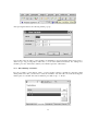
1.3
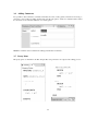
Creating a Project
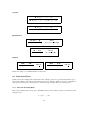
In order to create a new project, simply press the button as indicated below in the ”Project Explorer”
window:
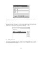
The following wizard will then appear, within which you type the name of the new project (here we type
”alpha”):
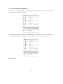
After pressing the ”Finish” button, the new project is created and appears in the ”Project Explorer” window.
1.4
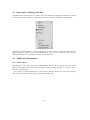
Removing a Project
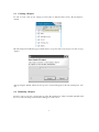
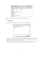
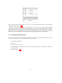
In order to remove a project, you first select it on the ”Project Explorer” window and then right click with
the mouse. The following contextual menu will appear on the screen:
3
You simply click on ”Delete” and your project will be deleted (confirmation is asked). It is then removed
from the Project Explorer window.
1.5
Exporting a Project
Exporting a project is the operation by which you can construct automatically a ”zip” file containing the
entire project. Such a file is ready to be sent by mail. Once received, an exported project can be imported
(next section), it then becomes a project like the other ones which were created locally. In order to export
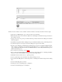
a project, first select it, and then press the ”File” button in the menubar as indicated below:
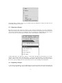
A menu will appear. You then press ”Export” on this menu. The Export wizard will pop up. In this
window, select ”Archive File” and click ”Next ¿”. Specify the path and name of the archive file into
which you want to export your project and finally click ”Finish”. This menu sequence belongs (as well as
the various options) to Eclipse. For more information, have a look at the Eclipse documentation.
1.6
Importing a Project
A ”.zip” file corresponding to a project which has been exported elsewhere can be imported locally. In
order to do that, click the ”File” button in the menubar (as done in the previous section). You then click
4
”Import” in the coming menu. In the import wizard, select ”Existing Projects into Workspace” and click
”Next ¿”. Then, enter the file name of the imported project and finally click ”Finish”. Like for exporting,
the menu sequence and layout are part of Eclipse.
The importation is refused if the name of the imported project (not the name of the file), is the same as
the name of an existing local project. The moral of the story is that when exporting a project to a partner
you better modify its name in case your partner has already got a project with that same name (maybe a
previous version of the exported project). Changing the name of a project is explained in the next section.
1.7
Changing the Name of a Project
The procedure for changing the name of a project is a bit heavy at the present time. Here is what you
have to do. Select the project whose name you want to modify. Enter the Eclipse ”Resource” perspective.
A ”Navigator” window will appear in which the project names are listed (and your project still selected).
Right click with the mouse and, in the coming menu, click ”Rename”. Modify the name and press enter.
Return then to the original perspective. The name of your project has been modified accordingly.
1.8
Creating a Component
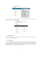
In this section, we learn how to create a component (context or machine). In order to create a component
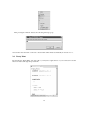
in a project, you have to first select the project and then click the corresponding button as shown below:
You may now choose the type of the component (machine or context) and give it a name as indicated:
5
Click ”Finish” to eventually create the component. The new component will appear in the Project Explorer
window.
1.9
Removing a Component
In order to remove a component, press the right mouse button. In the coming menu, click ”Delete”. This
component is removed from the Project Explorer window.
In the next two sections we describe in details first the contexts and then the machines.
2
Anatomy of a Context
Once a context is created, a window such as the following appears in the editing area (usually next to the
center of the screen):
6
It shows that a context is made of various components, namely dependencies, carrier sets, constants,
axioms, or theorems.
In the next sections we are going to see how to create, modify or remove such components. The creation
of these components. except dependencies (studied in section 2.7), can be made by two distinct methods,
either by using wizards or by editing them directly. In each section, we shall review both methods.
2.1
2.1.1
Carrier Sets
Carrier Sets Creation Wizard.
In order to activate the carrier set creation wizard, you have to press the corresponding button in the
toolbar as indicated below:
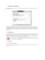
After pressing that button, the following wizard pops up:
You can enter as many carrier sets as you want by pressing the ”More” button. When you’re finished,
press the ”OK” button.
2.1.2
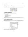
Direct Editing of Carrier Sets.
It is also possible to create (button ”Add”) or remove (button ”Delete”) carrier sets by using the central
editing window (see window below). For this, you have first to select the ”Carrier Sets” tab of the editor.
Notice that you can change the order of carrier sets: first select the carrier set and then press button ”Up”
or ”Down”.
7
As can be seen, we have created three carrier sets C, E, and D.
2.2
Enumerated Sets
In order to activate the enumerated set creation wizard, you have to press the corresponding button in the
toolbar as indicated below:
After pressing that button, the following wizard pops up:
8
You can enter the name of the new enumerated set as well as the name of its elements. By pressing the
button ”More Elements”, you can enter additional elements. When you’re finished, press the ”OK” button.
The effect of using this wizard as indicated is to add the new carrier set COLOR (section 2.1) and the
three constants (section 2.3) red, green, and orange. Finally, it adds the following axioms (section 2.4):
COLOR = {red, green, orange}
red 6= green
red 6= orange
green 6= orange
If you enter several time the same enumerated set element, you get an error message.
2.3
2.3.1
Constants
Constants Creation Wizard.
In order to activate the constants creation wizard, you have to press the corresponding button in the toolbar
as indicated below:
After pressing that button, the following wizard pops up:
You can then enter the names of the constants, and an axiom which can be used to define its type. Here is
an example:
9
By pressing the ”More Axm.” button you can enter additional axioms. For adding more constants, press
”Add” button. When you’re finished, press button ”OK”.
2.3.2
Direct Editing of Constants.
It is also possible to create (button ”Add”) or remove (button ”Delete”) constants by using the central
editing window. For this, you have first to select the ”Constants” tab of the editor. You can also change
the relative place of a constant: first select it and then press button ”Up” or ”Down”.
As can be seen, two more constants, bit1 and bit2 have been added. Note that this time the axioms
concerning these constants have to be added directly (see next section 2.4).
10
2.4
2.4.1
Axioms
Axioms Creation Wizard.
In order to activate the axioms creation wizard, you have to press the corresponding button in the toolbar
as indicated below:
After pressing that button, the following wizard appears:
You can then enter the axioms you want. If more axioms are needed then press ”More”. When you are
finished, press ”OK”.
2.4.2
Direct Editing of Axioms.
It is also possible to create (button ”Add”) or remove (button ”Delete”) axioms by using the central editing
window. For this, you have first to select the ”Axioms” tab of the editor. You can also change the relative
place of an axiom: first select it and then press button ”Up” or ”Down”.
11
Note that the ”Up” and ”Down” buttons for changing the order of axioms are important for welldefinedness. For example the following axioms in that order
axm1 : y/x = 3
axm2 : x 6= 0
does not allow to prove the well-definedness of y/x = 3. The order must be changed to the following:
axm2 : x 6= 0
axm1 : y/x = 3
The same remark applies to theorems (section 2.5 and 3.4), invariants (section 3.3) and event guards
(section3.5.2)
2.5
2.5.1
Theorems
Theorems Creation Wizard.
In order to activate the theorems creation wizard, you have to press the corresponding button in the toolbar
as indicated below:
After pressing that button, the following wizard pops up:
12
You can then enter the theorems you want. If more theorems are needed then press ”More”. When you
are finished, press ”OK”.
2.5.2
Direct Editing of Theorems.
It is also possible to create (button ”Add”) or remove (button ”Delete”) theorems by using the central
editing window. For this, you have first to select the ”Theorems” tab of the editor. You can also change
the relative place of a theorem: first select it and then press button ”Up” or ”Down”.
2.6
Adding Comments
It is possible to add comments to carrier sets, constants, axioms and theorems. For doing so, select the
corresponding modeling element and enter the ”Properties” window as indicated below where it is shown
how to add comments on a certain axiom:
13
Multiline comments can be added in the editing area labeled ”Comments”.
2.7
Dependencies
By selecting the ”Dependencies” tab of the editor, you obtain the following window:
This allows you to express that the current context is extending other contexts of the current project. In
order to add the name of the context you want to extend, use the combobox which appears at the bottom
of the window and then select the corresponding context name.
There exists another way to directly create a new context extending an existing context C. Select the
context C in the project window, then press the right mouse key, you’ll get the following menu:
14
After pressing the ”Extend” button, the following wizard pops up:
You can then enter the name of the new context which will be made automatically an extension of C.
2.8
Pretty Print
By selecting the ”Pretty Print” tab of the editor, you may have a global view of your context as if it would
have been entered through an input text file.
15
3
Anatomy of a Machine
Once a machine is created, a window such as the following appears in the editing area (usually next to the
center of the screen):
It shows that a machine is made of various components, namely dependencies, variables, invariants, theorems, variant, and events. In the next sections, we are going to see how to create, modify or remove
such components. Except for the dependencies, the creation of these components can be made by two
distinct methods, either by using wizards or by editing them directly. In each section, we shall review
both methods.
3.1
Dependencies
The ”Dependencies” window is shown automatically after creating a machine (you can also get it by
selecting the ”Dependencies” tab). This was shown in the previous section so that we do not copy the
screen shot again. As can be seen on this window, two kinds of dependencies can be established: machine
dependency in the upper part and context dependencies in the lower part.
In this section, we only speak of context dependencies (machine dependency will be covered in section 3.8). It corresponds to the ”sees” relationship alluded in section 1. In the lower editing area, you can
select some contexts ”seen” by the current machine.
3.2
3.2.1
Variables
Variables Creation Wizard.
In order to activate the variables creation wizard, you have to press the corresponding button in the toolbar
as indicated below:
16
After pressing that button, the following wizard pops up:
You can then enter the names of the variables, its initialization, and an invariant which can be used to
define its type. By pressing button ”More Inv.” you can enter additional invariants. For adding more
variables, press the ”Add” button. When you’re finished, press the ”OK” button.
3.2.2
Direct Editing of Variables.
It is also possible to create (button ”Add”) or remove (button ”Delete”) variables by using the central
editing window. For this, you have first to select the ”Variables” tab of the editor. You can also change the
relative place of a variable: first select it and then press button ”Up” or ”Down”.
17
3.3
3.3.1
Invariants
Invariants Creation Wizard.
In order to activate the invariants creation wizard, you have to press the corresponding button:
After pressing that button, the following wizard pops up:
You can then enter the invariants you want. If more invariants are needed then press ”More”.
3.3.2
Direct Editing of Invariants.
It is also possible to create (button ”Add”) or remove (button ”Delete”) invariants by using the central
editing window. For this, you have first to select the ”Invariants” tab of the editor. You can also change
the relative place of an invariant: first select it and then press button ”Up” or ”Down”.
18
3.4
3.4.1
Theorems
Theorems Creation Wizard.
In order to activate the theorems creation wizard, you have to press the corresponding button:
After pressing that button, the following wizard pops up:
You can then enter the theorems you want. If more theorems are needed then press ”More”. When you
are finished, press the ”OK” button.
3.4.2
Direct Editing of Theorems.
It is also possible to create (button ”Add”) or remove (button ”Delete”) theorems by using the central
editing window. For this, you have first to select the ”Theorems” tab of the editor. You can also change
the relative place of a theorem: first select it and then press button ”Up” or ”Down”.
19
3.5
3.5.1
Events
Events Creation Wizard.
In order to activate the events creation wizard, you have to press the corresponding button in the toolbar
as indicated below:
After pressing that button, the following wizard pops up:
You can then enter the events you want. As indicated, the following elements can be entered: name,
parameters, guards, and actions. More parameters, guards and actions can be entered by pressing the
corresponding buttons. If more events are needed then press ”Add”. Press ”OK” when you’re finished.
Note that an event with no guard is considered to have a true guard. Moreover, an event with no action
is considered to have the ”skip” action.
20
3.5.2
Direct Editing of Events.
It is also possible to perform a direct creation (button ”Add Event”) of variables by using the central
editing window. For this, you have first to select the ”Events” tab of the editor. You can also change the
relative place of a variable: first select it and then press button ”Up” or ”Down”.
Once an event is selected you can add parameters, guards, and actions. The components of an events can
be seen by pressing the little triangle situated on the left of the event name:
As can be seen, event rmv 1 is made of two parameters, x and y, three guards, x ∈ Q, y ∈ Q, and
x 7→ y ∈ k, and one action Q := Q \ {x}. These elements can be modified (select and edit) or removed
(select, right click on the mouse, and press ”Delete”). Similar elements can be added by pressing the
relevant buttons on the right of the window.
21
3.6
Adding Comments
It is possible to add comments to variables, invariants, theorems, events, guards, and actions. For doing so,
select the corresponding modeling element and enter the ”Properties” window as indicated below where
it is shown how one can add comments on a certain guard:
Multiline comments can be added in the editing area labeled ”Comments”.
3.7
Pretty Print
The pretty print of a machine looks like an input file. It is produced as an output of the editing process:
22
3.8
Dependencies: Refining a Machine
A machine can be refined by other ones. This can be done directly by selecting the machine to be refined
in the ”Project Explorer” window. A right click on the mouse yields the following contextual menu:
You then press button ”Refine”. A wizard will ask you to enter the name of the refined machine. The
abstract machine is entirely copied in the refined machine: this is very convenient as, quite often, the
refined machine has lots of elements in common with its abstraction.
3.9
3.9.1
Adding more Dependencies
Abstract Event
The absraction of an event is denoted by a ”Refine Event” element. Most of the time the concrete and
abstract events bear the same name. But, it is always possible to change the name of a concrete event or
the name of its abstraction.
If you want to specify the abstraction of an event, first select the ”Event” tab of the editor and right
click on the event name. The following contextual menu will pop up:
23
You have then to choose the ”New Refine Event” option. The abstract event can then be entered by adding
the name of the abstract event: here rmv 1.
3.9.2
Splitting an Event
An abstract event can be split into two or more concrete events by just saying that these events refine the
former (as explained in previous section).
3.9.3
Merging Events
Two or more abstract events can be merged into a single concrete event by saying that the latter refines
all the former. This is done by using several times the approach explained in the previous case. The
constraints is that the abstract events to be merged must have exactly the same actions (including the
labels of these actions). A proof obligation is generated which states that the guard of the concrete event
implies the disjunction of the guards of the abstract events
24
3.9.4
Witnesses
When an abstract event contains some parameters, the refinement proof obligation involves proving an
existentially quantified statement. In order to simplify the proof, the user is required to give witnesses
for those abstract parameters which are not present in the refinement (those appearing in the refinement
are implicitly taken as witnesses for their corresponding abstract counterparts). Here is an example of an
abstract event (left) and its refinement (right):
The parameter x, being common to both the abstraction and the refinement, does not require a witness,
whereas one is needed for abstract parameter y. In order to define the witness, one has first to select the
”Events” tab of the editor for the concrete machine where the concrete event (here rmv 1) is selected.
After a right click, a menu appears in the window as indicated:
You press button ”New Witness” and then you enter the parameter name (here y) and a predicate involving
y (here y = b) as indicated below
25
Most of the time, the predicate is an equality as in the previous example, meaning that the parameter is
defined in a deterministic way. But it can also be any predicate, in which case the parameter is defined in
a non-deterministic way.
3.9.5
Variant
New events can be defined in a concrete machine. Such events have no abstract counterparts. They must
refine the implicit ”empty” abstract event which does nothing.
Some of the new events can be selected to decrease a variant so that they do not take control for ever.
Such events are said to be CONVERGENT. In order to make a new event CONVERGENT, select it in the
”Events” tab and open the ”Properties” window. You can edit the ”conv.” area. There are three options:
ORDINARY (the default), CONVERGENT, or ANTICIPATED. The latter corresponds to a new event
which is not yet declared to be CONVERGENT but will be in a subsequent refinement.
In order to define the variant, use the variant wizard as shown below:
After pressing that button, the following wizard will pop up
26
You can enter the variant and then press ”OK”. The variant is either a natural number expression or a
finite set expression.
4
Saving a Context or a Machine
Once a machine or context is (possibly partly only) edited, you can save it by using the following button:
4.1
Automatic Tool Invocations
Once a ”Save” is done, three tools are called automatically, these are:
• the Static Checker,
• the Proof Obligation Generator,
• the Auto-Prover.
This can take a certain time. A ”Progress” window can be opened at the bottom right of the screen to see
which tools are working (most of the time, it is the auto-prover).
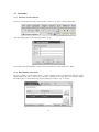
4.2
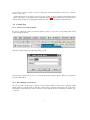
Errors. The Problems Window
When the Static Checker discovers an error in a project, a little ”x” is added to this project and to the
faulty component in the ”Project Explorer” window as shown in the following screen shot:
The error itself is shown by opening the ”Problems” window.
27
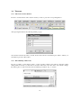
By double-clicking on the error statement, you are transferred automatically into the place where the error
has been detected so that you can correct it easily as shown below:
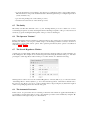
5
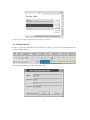
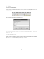
The Proof Obligation Explorer
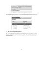
The ”Proof Obligation Explorer” window has the same main entries as the ”Project Explorer” window,
namely the projects and its components (context and machines). When expanding a component in the
Proof Obligation Explorer you get a list of its proof obligations as generated automatically by the Proof
Obligation Generator:
28
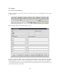
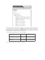
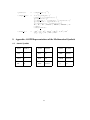
As can be seen in this screen shot, machine ”celebrity 1” of project ”celebrity” is expanded. We find seven
proof obligations. Each of them has got a compound name as indicated in the tables below. A green logo
situated on the left of the proof obligation name states that it has been proved (an A means it has been
proved automatically). By clicking on the proof obligation name, you are transferred into the Proving
Perspective which we are going to describe in subsequent sections.
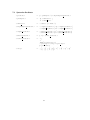
Next is a table describing the names of context proof obligations:
Well-definedness of an Axiom
axm / WD
axm is the axiom name
Well-definedness of a Theorem
thm / WD
thm is the theorem name
Theorem
thm / THM
thm is the theorem name
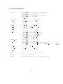
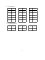
Next is a table showing the name of machine proof obligations:
29
Well-definedness of an Invariant
inv / WD
inv is the invariant name
Well-definedness of a Theorem
thm / WD
thm is the theorem name
Well-definedness of an event Guard
evt / grd / WD
evt is the event name
grd is the action name
Well-definedness of an event Action
evt / act / WD
evt is the event name
act is the action name
Feasibility of a non-det. event Action
evt / act / FIS
evt is the event name
act is the action name
Theorem
thm / THM
thm is the theorem name
Invariant Establishment
INIT. / inv / INV
inv is the invariant name
Invariant Preservation
evt / inv / INV
evt is the event name
inv is the invariant name
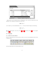
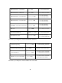
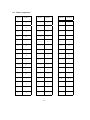
Next are the proof obligations concerned with machine refinements:
evt is the concrete event name
grd is the abstract guard name
Guard Strengthening
evt / grd / GRD
Guard Strengthening (merge)
evt / MRG
Action Simulation
evt / act / SIM
evt is the concrete event name
act is the abstract action name
Equality of a preserved Variable
evt / v / EQL
evt is the concrete event name
v is the preserved variable
evt is the concrete event name
Next are the proof obligations concerned with the new events variant:
30
Well definedness of Variant
VWD
Finiteness for a set Variant
FIN
Natural number for a numeric Variant
evt / NAT
evt is the new event name
Decreasing of Variant
evt / VAR
evt is the new event name
Finally, here are the proof obligations concerned with witnesses:
Well definedness of Witness
evt / p / WWD
evt is the concrete event name
p is parameter name
or a primed variable name
Feasibility of non-det. Witness
evt / p / WFIS
evt is the concrete event name
p is parameter name
or a primed variable name
Remark: At the moment, the deadlock freeness proof obligation generation is missing. If you need it, you
can generate it yourself as a theorem saying the the disjunction of the abstract guards imply the disjunction
of the concrete guards.
6
The Proving Perspective
The Proving Perspective is made of a number of windows: the proof tree, the goal, the selected hypotheses,
the proof control, the proof information, and the searched hypotheses. In subsequent sections, we study
these windows, but before that let us see how one can load a proof.
6.1
Loading a Proof
In order to load a proof, enter the Proof Obligation window, select the project, select and expand the
component, finally select the proof obligation: the corresponding proof will be loaded. As a consequence:
• the proof tree is loaded in the Proof Tree window. As we shall see in section 6.2, each node of the
proof tree is associated with a sequent.
• In case the proof tree has some ”pending” nodes (whose sequents are not discharged yet) then the
sequent corresponding to the first pending node is decomposed: its goal is loaded in the Goal window (section 6.3), whereas parts of its hypotheses (the ”selected” ones) are loaded in the Selected
Hypotheses window (section 6.3).
• In case the proof tree has no pending node, then the sequent of the root node is loaded as explained
previously.
31
6.2
6.2.1
The Proof Tree
Description of the Proof Tree
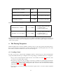
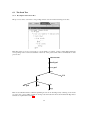
The proof tree can be seen in the corresponding window as shown in the following screen shot:
Each line in the proof tree corresponds to a node which is a sequent. A line is right shifted when the
corresponding node is a direct descendant of the node of the previous line. Here is an illustration of the
previous tree:
auto rewrite
forall goal
==> goal
ovr
eh
PP
ah
T goal
eh
ML
hyp
Each node is labelled with a comment explaining how it can be discharged. By selecting a node in the
proof tree, the corresponding sequent is decomposed and loaded in the Goal and Selected Hypotheses
windows as explained in section 6.1.
32
6.2.2
Decoration
The leaves of the tree are decorated with three kinds of logos:
√
• a green logo with a ” ” in it means that this leaf is discharged,
• a red logo with a ”?” in it means that this leaf is not discharged,
• a blue logo with a ”R” in it means that this leaf has been reviewed.
Internal nodes in the proof tree are decorated in the same (but lighter) way.
6.2.3
Navigation within the Proof Tree
On top of the proof tree window one can see three buttons:
• the ”G” buttons allows you to see the goal of the sequent corresponding to the node
• the ”+” button allows you to fully expand the proof tree
• the ”-” allows you to fully collapse the tree: only the root stays visible.
6.2.4
Hiding
The little triangle next to each node in the proof tree allows you to expand or collapse the subtree starting
at that node.
6.2.5
Pruning
The proof tree can be pruned from a node: it means that the subtree starting at that node is eliminated.
The node in question becomes a leaf and is red decorated. This allows you to resume the proof from that
node. After selecting a sequent in the proof tree, pruning can be performed in two ways:
• by right-clicking and then selecting ”Prune”,
• by pressing the ”Scissors” button in the proof control window (section 6.4).
Note that after pruning, the post-tactic is not applied to the new current sequent: if needed you have
to press the ”post-tactic” button in the Proof Control window (section 6.4). This happens in particular
when you want to redo a proof from the beginning: you prune the proof tree from the root node and then
you have to press the ”post-tactic” button in order to be in exactly the same situation as the one delivered
automatically initially.
When you want to redo a proof from a certain node, it might be advisable to do it after copying the
tree so that in case your new proof fails you can still resume the previous situation by pasting the copied
version (see next section).
6.2.6
Copy/Paste
By selecting a node in the proof tree and then clicking on the right key of the mouse, you can copy the
part of the proof tree starting at that sequent: it can later be pasted in the same way. This allows you to
reuse part of a proof tree in the same (or even another) proof.
33
6.3
Goal and Selected Hypotheses
The ”Goal” and ”Selected Hypotheses” windows display the current sequent you have to prove at a given
moment in the proof. Here is an example:
A selected hypothesis can be deselected by first clicking in the box situated next to it (you can click on
several boxes) and then by pressing the red (-) button at the top of the selected hypothesis window:
Here is the result:
34
Notice that the deselected hypotheses are not lost: you can get them back by means of the Searched
Hypotheses window (section 6.7).
The three other buttons next to the red (-) button allow you to do the reverse operation, namely keeping
some hypotheses. The (ct) button next to the goal allows you to do a proof by contradiction: pressing it
makes the negation of the goal being a selected hypothesis whereas the goal becomes ”false”. The (ct)
button next to a selected hypothesis allows you to do another kind of proof by contradiction: pressing it
makes the negation of the hypothesis the goal whereas the negated goal becomes an hypothesis.
6.4
The Proof Control Window
The Proof Control window contains the buttons which you can use to perform an interactive proof. Next
is a screen shot where you can see successively from top to bottom:
• some selected hypotheses,
• the goal,
• the ”Proof Control” window,
• a small editing area within which you can enter parameters used by some buttons of the Proof
Control window
• the smiley (section 6.5)
35
The Proof Control window offers a number of buttons which we succinctly describe from left to right:
• (p0): the prover PP attempts to prove the goal (other cases in the list)
• (R) review: the user forces the current sequent to be discharged, it is marked as being reviewed (it’s
logo is blue-colored)
• (dc) proof by cases: the goal is proved first under the predicate written in the editing area and then
under its negation,
• (ah) lemma: the predicate in the editing area is proved and then added as a new selected hypothesis,
• (ae) abstract expression: the expression in the editing area is given a fresh name,
• the auto-prover attempts to discharge the goal. The auto-prover is the one which is applied automatically on all proof obligations (as generated automatically by the proof obligation generator after a
”save”) without any intervention of the user. With this button, you can call yourself the auto-prover
within an interactive proof.
• the post-tactic is executed (see section 6.8),
• lasso: load in the Selected Hypotheses window those unseen hypotheses containing identifiers
which are common with identifiers in the goal and selected hypotheses,
• backtrack form the current node (i.e., prune its parent),
• scissors: prune the proof tree from the node selected in the proof tree,
• show (in the Search Hypotheses window) hypotheses containing the character string as in the editing
area,
• show the Cache Hypotheses window,
• load the previous non-discharged proof obligation,
• load the next undischarged proof obligation,
36
• (i) show information corresponding to the current proof obligation in the corresponding window.
This information correspond to the elements that took directly part in the proof obligation generation
(events, invariant, etc.),
• goto the next pending node of the current proof tree,
• load the next reviewed node of the current proof tree.
6.5
The Smiley
The smiley can take three different colors: (1) red, meaning that the proof tree contains one or more
non-discharged sequents, (2) blue, meaning that all non-discharged sequents of the proof tree have been
reviewed, (3) green, meaning that all sequents of the proof tree are discharged.
6.6
The Operator ”Buttons”
In the goal and in the selected, searched, or cache hypotheses some operators are colored in red. It means
that they are ”buttons” you can press. When doing so, the meaning (sometimes several) is shown in a
menu where you can select various options. The operation performed by these options is described in
sections 6.9.1 and 6.9.2.
6.7
The Search Hypotheses Window
A window is provided which contains the hypotheses having a character string in common with the one
in the editing area. For example, if we search for hypotheses involving the character string ”cr”, then after
pressing the ”search hypothesis” button in the proof control window, we obtain the following:
Such hypotheses can be moved to the ”Selected Hypotheses” window (button (+)) or removed from the
”Search Hypotheses” window (button (-)). As for the selected hypotheses, other buttons situated next to
the previous ones, allow you to move or remove all hypotheses. By pressing the (ct) button the negation
of the corresponding hypothesis becomes the new goal.
6.8
The Automatic Post-tactic
In this section, we present the various re-writing or inference rules which are applied automatically as
a systematic post-tactic after each proof step. Note that the post-tactic can be disabled by using the ”P
/”
button situated on the right of the proof control window.
37
The post-tactic is made of two different rules: rewrite rules, which are applied on any sub-formula
of the goal or selected hypotheses (section 6.8.1) and inference rules which are applied on the current
sequent (section 6.8.2).
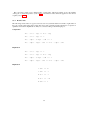
6.8.1
Rewrite rules
The following rewrite rules are applied automatically in a systematic fashion from left to right either in
the goal or in the selected hypotheses. They all correspond to predicate logical equivalences or expression
equalities and result in simplifications. They are sorted according to their main purpose.
Conjunction
P ∧ . . . ∧ > ∧ . . . ∧ Q == P ∧ . . . ∧ Q
P ∧ . . . ∧ ⊥ ∧ . . . ∧ Q == ⊥
P ∧ . . . ∧ Q ∧ . . . ∧ ¬ Q ∧ . . . ∧ R == ⊥
P ∧ . . . ∧ Q ∧ . . . ∧ Q ∧ . . . ∧ R == P ∧ . . . ∧ Q ∧ . . . ∧ R
Disjunction
P ∨ . . . ∨ > ∨ . . . ∨ Q == >
P ∨ . . . ∨ ⊥ ∨ . . . ∨ Q == P ∨ . . . ∨ Q
P ∨ . . . ∨ Q ∨ . . . ∨ ¬ Q ∨ . . . ∨ R == >
P ∨ . . . ∨ Q ∨ . . . ∨ Q ∨ . . . ∨ R == P ∨ . . . ∨ Q ∨ . . . ∨ R
Implication
> ⇒ P == P
⊥ ⇒ P == >
P ⇒ > == >
P ⇒ ⊥ == ¬ P
P ⇒ P == >
38
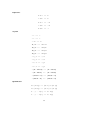
Equivalence
P ⇔ > == P
> ⇔ P == P
P ⇔ ⊥ == ¬ P
⊥ ⇔ P == ¬ P
P ⇔ P == >
Negation
¬ > == ⊥
¬ ⊥ == >
¬ ¬ P == P
E 6= F == ¬ E = F
E∈
/ F == ¬ E ∈ F
E 6⊂ F == ¬ E ⊂ F
E 6⊆ F == ¬ E ⊆ F
¬ a ≤ b == a > b
¬ a ≥ b == a < b
¬ a > b == a ≤ b
¬ a < b == a ≥ b
¬ (E = FALSE) ==
(E = TRUE)
¬ (E = TRUE) ==
(E = FALSE)
¬ (FALSE = E) ==
(TRUE = E)
¬ (TRUE = E) ==
(FALSE = E)
Quantification
∀x · ( P ∧ Q) == (∀x · P ) ∧ (∀x · Q)
∃x · ( P ∨ Q) == (∃x · P ) ∨ (∃x · Q)
∀ . . . , z, . . . · P (z) == ∀z · P (z)
∃ . . . , z, . . . · P (z) == ∃z · P (z)
39
Equality
E = E == >
E 6= E == ⊥
E 7→ F = G 7→ H == E = G ∧ F = H
TRUE = FALSE ==
⊥
FALSE = TRUE ==
⊥
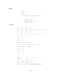
Set Theory
S ∩ . . . ∩ ∅ ∩ . . . ∩ T == ∅
S ∩ . . . ∩ T ∩ . . . ∩ T ∩ . . . ∩ U == S ∩ . . . ∩ T ∩ . . . ∩ U
S ∪ . . . ∪ ∅ ∪ . . . ∪ T == S ∪ . . . ∪ T
S ∪ . . . ∪ T ∪ . . . ∪ T ∪ . . . ∪ U == S ∪ . . . ∪ T ∪ . . . ∪ U
∅ ⊆ S == >
S ⊆ S == >
E ∈ ∅ == ⊥
B ∈ {A, . . . , B, . . . , C} == >
{A, . . . , B, . . . , B, . . . , C} == {A, . . . , B, . . . , C}
E ∈ { x | P (x) } == P (E)
S \ S == ∅
S \ ∅ == S
∅ \ S == ∅
r−1−1 == r
dom({x 7→ a, . . . , y 7→ b} == {x, . . . , y}
ran({x 7→ a, . . . , y 7→ b} == {a, . . . , b}
(f − ... − {E 7→ F })(E) == F
E ∈ {F } == E = F
where F is a single expression
40
{E} = {F } == E = F
where E and F are single expressions
{x 7→ a, . . . , y 7→ b}−1 == {a 7→ x, . . . , b 7→ y}
T y = ∅ == ⊥
∅ = T y == ⊥
t ∈ T y == >
In the three previous rewrite rules, T y denotes a type expression, that is either a basic type (Z, BOOL,
any carrier set), or P(type expression), or type expression×type expression, and t denotes an expression
of type T y.
U \ U \ S == S
S ∪ . . . ∪ U ∪ . . . ∪ T == U
S ∩ . . . ∩ U ∩ . . . ∩ T == S ∩ . . . ∩ T
S \ U == ∅
In the four previous rules, S and T are supposed to be of type P(U ).
r ; ∅ == ∅
∅ ; r == ∅
f (f −1 (E)) == E
f −1 (f (E)) == E
Arithmetic
E + . . . + 0 + . . . + F == E + . . . + F
E − 0 == E
0 − E == −E
−(−E) == E
E ∗ . . . ∗ 1 ∗ . . . ∗ F == E ∗ . . . ∗ F
E ∗ . . . ∗ 0 ∗ . . . ∗ F == 0
(−E) ∗ . . . ∗ (−F ) == E ∗ . . . ∗ F
(if an even number of -)
(−E) ∗ . . . ∗ (−F ) == − (E ∗ . . . ∗ F )
(if an odd number of -)
41
E/1 == E
0/E == 0
(−E)/(−F ) == E/F
E 1 == E
E 0 == 1
1E == 1
−(i) == (−i) where i is a literal
−((−i)) == i where i is a literal
i = j == > or ⊥ (computation)
where i and j are literals
i ≤ j == > or ⊥ (computation)
where i and j are literals
i < j == > or ⊥ (computation)
where i and j are literals
i ≥ j == > or ⊥ (computation)
where i and j are literals
i > j == > or ⊥ (computation)
where i and j are literals
E ≤ E == >
E < E == ⊥
E ≥ E == >
E > E == ⊥
6.8.2
Automatic inference rules
The following inference rules are applied automatically in a systematic fashion at the end of each proof
step. They have the following possible effects:
• they discharge the goal,
• they simplify the goal and add a selected hypothesis,
• they simplify the goal by decomposing it into several simpler goals,
• they simplify a selected hypothesis,
• they simplify a selected hypothesis by decomposing it into several simpler selected hypotheses.
42
Axioms
HYP
H, P ` P
H, Q ` P ∨ . . . ∨ Q ∨ . . . ∨ R
H, P, ¬ P ` Q
CNTR
FALSE HYP
H, ⊥ ` P
HYP OR
TRUE GOAL
H ` >
Simplification
H, P ` Q
H, P, P ` Q
DBL HYP
Conjunction
H, P, Q ` R
H, P ∧ Q ` R
H ` P
AND L
H ` Q
H ` P ∧ Q
AND R
Implication
H, Q, P ∧ . . . ∧ R ⇒ S ` T
H, Q, P ∧ . . . ∧ Q ∧ . . . ∧ R ⇒ S ` T
IMP L1
H, P ` Q
H ` P⇒Q
H, P ⇒ Q, P ⇒ R ` S
H, P ⇒ Q ∧ R ` S
IMP R
H, P ⇒ R, Q ⇒ R ` S
IMP AND L
H, P ∨ Q ⇒ R ` S
43
IMP OR L
Negation
H, E ∈ {a, . . . , c} `
P
H, E ∈ {a, . . . , b, . . . , c}, ¬ (E = b) ` P
H, E ∈ {a, . . . , c} `
P
H, E ∈ {a, . . . , b, . . . , c}, ¬ (b = E) ` P
Quantification
H, P(x) ` Q
XST L
(x not free in H and Q)
H, ∃ x · P(x) ` Q
H ` P(x)
ALL R
(x not free in H)
H ` ∀x · P(x)
Equality
H(E) `
H(E) `
P(E)
H(x), x = E ` P(x)
EQL LR
P(E)
H(x), E = x ` P(x)
EQL RL
In these two rules x is a variable which is not free in E
6.9
Interactive Tactics
In this section, the rewriting rules and inference rules, which you can use to perform an interactive proof,
are presented. Each of these rules can be invoked by pressing ”buttons” which corresponds to emphasized
(red) operators in the goal or the hypotheses. A menu is proposed when there are several options.
6.9.1
Interactive Rewriting Rules
Most of the rewriting rules correspond to distributive laws. For associative operators in connection with
such laws as in:
P ∧ (Q ∨ . . . ∨ R)
44
it has been decided to put the ”button” on the first associative/commutative operator (here ∨). Pressing that
button will generate a menu: the first option of this menu will be to distribute all associative/commutative
operators, the second option will be to distribute only the first associative/commutative operator. In the
following presentation, to simplify matters, we write associative/commutative operators with two parameters only, but it must always be understood implicitly that we have a sequence of them. For instance, we
shall never write Q ∨ . . . ∨ R but Q ∨ R instead. Rules are sorted according to their purpose.
Conjunction
P ∧ (Q ∨ R) == (P ∧ Q) ∨ (P ∧ R)
Disjunction
P ∨ (Q ∧ R) == (P ∨ Q) ∧ (P ∨ R)
P ∨ Q ∨ . . . ∨ R == ¬ P ⇒ (Q ∨ . . . ∨ R)
Implication
P ⇒ Q == ¬ Q ⇒ ¬P
P ⇒ (Q ⇒ R) == P ∧ Q ⇒ R
P ⇒ (Q ∧ R) == (P ⇒ Q) ∧ (P ⇒ R)
P ∨ Q ⇒ R == (P ⇒ R) ∧ (Q ⇒ R)
Equivalence
P ⇔ Q == (P ⇒ Q) ∧ (Q ⇒ P )
Negation
¬ (P ∧ Q) == ¬ P ∨ ¬ Q
¬ (P ∨ Q) == ¬ P ∧ ¬ Q
¬ (P ⇒ Q) == P ∧ ¬ Q
¬ ∀x · P == ∃x · ¬ P
¬ ∃x · P == ∀x · ¬ P
¬ (S = ∅) == ∃x · x ∈ S
Set Theory
Most of the rules are concerned with simplifying set membership predicates.
45
E 7→ F ∈ S × T == E ∈ S ∧ F ∈ T
E ∈ P(S) == E ⊆ S
S ⊆ T == ∀x · ( x ∈ S ⇒ x ∈ T )
In the previous rule, x denotes several variables when the type of S and T is a Cartesian product.
E ∈ S ∪ T == E ∈ S ∨ E ∈ T
E ∈ S ∩ T == E ∈ S ∧ E ∈ T
E ∈ S \ T == E ∈ S ∧ ¬ (E ∈ T )
E ∈ {A, . . . , B}
==
E = A ∨ ... ∨ E = B
E ∈ union (S) == ∃s · s ∈ S ∧ E ∈ s
S
E ∈ ( x · x ∈ S ∧ P | T ) == ∃x · x ∈ S ∧ P ∧ E ∈ T
E ∈ inter (S) == ∀s · s ∈ S ⇒ E ∈ s
T
E ∈ ( x · x ∈ S ∧ P | T ) == ∀x · x ∈ S ∧ P ⇒ E ∈ T
E ∈ dom(r) == ∃y · E 7→ y ∈ r
F ∈ ran(r) == ∃x · x 7→ F ∈ r
E 7→ F ∈ r−1 == F 7→ E ∈ r
E 7→ F ∈ S r == E ∈ S ∧ E 7→ F ∈ r
E 7→ F ∈ r T == E 7→ F ∈ r ∧ F ∈ T
E 7→ F ∈ S − r == E ∈
/ S ∧ E 7→ F ∈ r
E 7→ F ∈ r − T == E 7→ F ∈ r ∧ F ∈
/T
F ∈ r[w] == ∃x · x ∈ w ∧ x 7→ F ∈ r
E 7→ F ∈ (p ; q) == ∃x · E 7→ x ∈ p ∧ x 7→ F ∈ q
p
− q == (dom (q) − p) ∪ q
E 7→ F ∈ id (S) == E ∈ S ∧ F = E
E 7→ (F 7→ G) ∈ p ⊗ q == E 7→ F ∈ p ∧ E 7→ G ∈ q
(E 7→ G) 7→ (F 7→ H) ∈ p k q == E 7→ F ∈ p ∧ G 7→ H ∈ q
46
r∈S←
↔ T == r ∈ S ↔ T ∧ dom(r) = S
r∈S↔
→ T == r ∈ S ↔ T ∧ ran(r) = T
r∈S↔
↔ T == r ∈ S ↔ T ∧ dom(r) = S ∧ ran(r) = T
f ∈S→
7 T == f ∈ S ↔ T ∧ ∀x, y, z·x 7→ y ∈ f ∧ x 7→ z ∈ f ⇒ y = z
f ∈ S → T == f ∈ S →
7 T ∧ dom(f ) = S
f ∈S
7 T == f ∈ S →
7 T ∧ f −1 ∈ T →
7 S
f ∈ S T == f ∈ S 7 T ∧ dom(f ) = S
f ∈S
7 T == f ∈ S →
7 T ∧ ran(f ) = T
f ∈ S T == f ∈ S 7 T ∧ dom(f ) = S
f ∈S
T == f ∈ S T ∧ ran(f ) = T
(p ∪ q)−1 == p−1 ∪ q −1
(p ∩ q)−1 == p−1 ∩ q −1
(s r)−1 == r−1 s
(s − r)−1 == r−1 −s
(r s)−1 == s r−1
(r − s)−1 == s r−1
(p ; q)−1 == q −1 ; p−1
(s ∪ t) r == (s r) ∪ (t r)
(s ∩ t) r == (s r) ∩ (t r)
(s ∪ t) − r == (s − r) ∩ (t − r)
(s ∩ t) − r == (s − r) ∪ (t − r)
s (p ∪ q) == (s p) ∪ (s q)
s (p ∩ q) == (s p) ∩ (s q)
s
− (p ∪ q) == (s − p) ∪ (s − q)
s
− (p ∩ q) == (s − p) ∩ (s − q)
47
r (s ∪ t) == (r s) ∪ (r t)
r (s ∩ t) == (r s) ∩ (r t)
r
− (s ∪ t) == (r − s) ∩ (r − t)
r
− (s ∩ t) == (r − s) ∪ (r − t)
(p ∪ q) s == (p s) ∪ (q s)
(p ∩ q) s == (p s) ∩ (q s)
(p ∪ q) − s == (p − s) ∪ (q − s)
(p ∩ q) − s == (p − s) ∩ (q − s)
r[S ∪ T ] == r[S] ∪ r[T ]
(p ∪ q)[S] == p[S] ∪ q[S]
dom(p ∪ q) == dom(p) ∪ dom(q)
ran(p ∪ q) == ran(p) ∪ ran(q)
S ⊆ T == (U \ T ) ⊆ (U \ S)
In the previous rule, the type of S and T is P(U ).
S = T == S ⊆ T ∧ T ⊆ S
In the previous rule, S and T are sets
p ; (q ∪ r) == (p ; q) ∪ (p ; r)
(q ∪ r) ; p == (q ; p) ∪ (r ; p)
(p ; q)[s] == q[p[s]]
(s p) ; q == s (p ; q)
(s − p) ; q == s − (p ; q)
p ; (q s) == (p ; q) s
p ; (q − s) == (p ; q) −s
U \ (S ∩ T ) == (U \ S) ∪ (U \ T )
U \ (S ∪ T ) == (U \ S) ∩ (U \ T )
U \ (S \ T ) == (U \ S) ∪ T
In the three previous rules, S and T are supposed to be of type P(U ).
48
6.9.2
Interactive Inference rules
Disjunction
H, P ` R
...
H, Q ` R
CASE
H, P ∨ . . . ∨ Q ` R
Implication
H ` P
H, P, Q ` R
MH
H, P ⇒ Q ` R
H ` ¬Q
H, ¬ Q, ¬ P ` R
HM
H, P ⇒ Q ` R
Equivalence
H(Q), P ⇔ Q ` G(Q)
H(P), P ⇔ Q ` G(P)
EQV
postponed
Set Theory
H, G = E, P(F ) ` Q
H, ¬ (G = E), P(f (G)) ` Q
H, P((f − {E 7→ F })(G)) ` Q
H, G = E ` Q(F )
H, ¬ (G = E) ` Q(f (G))
H ` Q((f − {E 7→ F })(G))
H, G ∈ dom(g), P(g(G)) ` Q
OV L
OV R
H, ¬ G ∈ dom(g), P(f (G)) ` Q
H, P((f − g)(G)) ` Q
49
OV L
H, G ∈ dom(g) ` Q(g(G))
H, ¬ G ∈ dom(g) ` Q(f (G))
OV R
H ` Q((f − g)(G))
In the four previous rules the − operator must appear at the ”top level”
H ` f −1 ∈ A →
7 B
H ` Q(f [S] ∩ f [T ])
H ` Q(f [S ∩ T ])
H ` f ∈A→
7 B
H ` Q(f −1 [S] \ f −1 [T ])
H ` Q(f −1 [S \ T ])
∩DIS R
\DIS R
In the two previous rules, the occurrence of f −1 must appear at the ”top level”. Moreover A and B denote
some type. Similar left distribution rules exist
H ` WD(Q({f (E)}))
H ` Q({f (E)})
H ` Q(f [{E}])
SIM R
In the previous rule, the occurrence of f must appear at the ”top level”. A similar left simplification rule
exists.
H ` WD(Q(g(f (x))))
H ` Q(g(f (x)))
H ` Q((f ; g)(x))
SIM R
In the previous rule, the occurrence of f ; g must appear at the ”top level”. A similar left simplification
rule exists.
7
Syntax of the Mathematical Language
In this section,we present the syntax of the mathematical language. It comprises two main syntactic
constructs, namely < predicate > (section 7.1) and < expression > (section 7.2).
50
7.1
Syntax for Predicates
< predicate >
::=
{< quantif ier >} < unquantif ied predicate >
< quantif ier >
::=
‘∀0 < ident list > ‘· 0
‘∃0 < ident list > ‘· 0
< ident list >
::=
< ident > {, < ident >}
< unquantif ied predicate >
::=
< simple predicate > [‘⇒0 < simple predicate >]
< simple predicate > [‘⇔0 < simple predicate >]
< simple predicate >
::=
< literal predicate > {‘∧0 < literal predicate >}
< literal predicate > {‘∨0 < literal predicate >}
< literal predicate >
::=
{‘¬0 } < atomic predicate >
< atomic predicate >
::=
‘⊥0
‘>0
‘ finite0 (< expression >)
< pair expr >< relop >< pair expr >
(< predicate >)
< relop >
::=
‘ =0 | ‘ 6=0 | ‘ ∈0 | ‘ ∈
/ | ‘ ⊂0 | ‘ 6⊂0 | ‘ ⊆0 | ‘ 6⊆0
0
0
0
‘ < | ‘ ≤ | ‘ > | ‘ ≥0
0
51
7.2
Syntax for Expressions
< expression >
::= ‘λS0 < ident pattern > ‘· 0 < predicate > ‘ |0 < expression >
0
‘ S < ident list > ‘· 0 < predicate > ‘ |0 < expression >
0
‘ T < expression > ‘ |0 < predicate >
0
‘ T < ident list > ‘· 0 < predicate > ‘ |0 < expression >
0
‘
< expression > ‘ |0 < predicate >
< pair expr >
< ident pattern >
::= < ident pattern > {‘ 7→0 < ident pattern >}
‘(0 < ident pattern > ‘)0
< ident >
< pair expr >
::= < rel set expr > {‘ 7→0 < rel set expr >}
< rel set expr >
::= < set expr > {< rel set op >< set expr >}
< rel set op >
::= ‘ ↔0 | ‘ ←
↔0 | ‘ ↔
→0 | ‘ ↔
↔0 | ‘ →
7 0 | ‘→0
0
0
0
0
‘
7
| ‘ | ‘
7
| ‘ | ‘
0
< set expr >
::= < interval
< interval
< interval
< interval
< interval
[< domain
< domain mod >
::= < interval expr > (‘ 0 | ‘
−0
< rel expr >
::= < interval expr > ‘⊗0 < interval expr >
< interval expr > {‘;0 < interval expr >}[< range mod >]
< interval expr > {‘∩ 0 < interval expr >}[‘\0 < interval expr > | < range mod >]
< range mod >
::= (‘ 0 | ‘
−0 ) < interval expr >
expr > {‘∪ 0 < interval expr >}
expr > {‘×0 < interval expr >}
expr > {‘
−0 < interval expr >}
expr > {‘◦0 < interval expr >}
expr > ‘k0 < interval expr >
mod >] < rel expr >
< interval expr > ::= < arith expr > [‘..0 < arith expr >]
< arith expr >
::= [‘−0 ] < term > {(‘ +0 | ‘−0 ) < term >}
< term >
::= < f actor > {(‘ ∗0 | ‘ ÷0 | ‘ mod 0 ) < f actor >}
< f actor >
::=
< image > [‘b0 < image >]
< image >
::=
< primary > {‘[0 < expression > ‘]0 | ‘(0 < expression > ‘)0 }
52
< primary >
0
::= < simple expr > {‘−1 }
< simple expr > ::= ‘ bool0 ‘(0 < predicate > ‘)0
< unary op > ‘(0 < expression > ‘)0
‘(0 < expression > ‘)0
‘{0 < ident list > ‘· 0 < predicate > ‘ |0 < expression > ‘}0
‘{0 < expression > ‘ |0 < predicate > ‘}0
‘{0 [< expression > {‘,0 < expression >}]‘}0
‘Z0 | ‘N0 | ‘N1 0 | ‘BOOL0 | ‘TRUE0 | ‘FALSE0 | ‘∅0
< ident >
< integer literal >
< unary op >
8
8.1
::= ‘ card0 | ‘ P0 | ‘ P1 0 | ‘ union0 | ‘ inter0 | ‘ dom0 | ‘ ran0
‘ prj1 0 | ‘ prj2 0 | ‘ id0 | ‘ min0 | ‘ max0
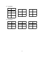
Appendix: ASCII Representations of the Mathematical Symbols
Atomic Symbols
ASCII
Symbol
ASCII
Symbol
ASCII
Symbol
true
>
NAT
N
TRUE
TRUE
false
⊥
NAT1
N1
FALSE
FALSE
INT
Z
BOOL
BOOL
{}
∅
53
8.2
8.3
Unary Operators
ASCII
Symbol
ASCII
Symbol
ASCII
Symbol
not
¬
union
union
prj2
prj2
finite
finite
inter
inter
id
id
card
card
dom
dom
min
min
POW
P
ran
ran
max
max
POW1
P1
prj1
prj1
-
−
ASCII
Symbol
ASCII
Symbol
Assignment Operators
ASCII
:=
Symbol
:=
:|
:|
54
::
:∈
8.4
Binary Operators
ASCII
Symbol
Symbol
ASCII
ASCII
Symbol
&
∧
|->
7→
<+
−
or
∨
<->
↔
||
k
=>
⇒
<<->
←
↔
><
⊗
<=>
⇔
<->>
↔
→
;
;
=
=
<<->>
↔
↔
<|
/=
6=
+->
→
7
<<|
−
:
∈
-->
→
|>
/:
∈
/
>+>
7
|>>
−
<<:
⊂
>->
+
+
/<<:
6⊂
+->>
7
-
−
<:
⊆
-->>
*
∗
/<:
6⊆
>->>
/
÷
<
<
/\
∩
mod
<=
≤
\/
∪
..
..
>
>
\
\
ˆ
b
>=
≥
**
×
˜
55
mod
−1
8.5
Quantifiers
ASCII
Symbol
Symbol
UNION
S
|
|
INTER
T
.
·
ASCII
Symbol
ASCII
Symbol
∀
!
∃
#
λ
%
8.6
ASCII
Bracketing
ASCII
Symbol
ASCII
Symbol
(
(
[
[
{
{
)
)
]
]
}
}
56