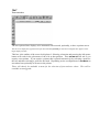
1
©
VORTEX -NT
USER MANUAL
FOR AIR FLOW, HEAT TRANSFER AND
CONCENTRATION IN ENCLOSURES
VERSION 3.10-005W
December 2001
VORTEX© is the copyright of Dr. H. B. Awbi
FLOWVIS© is the copyright of J.A. Ewer and Dr. M.K. Patel
Contents
Page
1.
INTRODUCTION
5
2.
REQUIREMENTS FOR USING VORTEX
6
3.
INSTALLATION AND RUNNING
7
4.
DESCRIPTION OF THE CFD MODEL
8
5.
MODELLING TECHNIQUES
9
INPUT PARAMETERS
FIRE SOURCE DATA
CREATING *.VDB FILE
6.
RUNNING VORTEX
RUN PAGE
OUTPUT FILES
7.
OTHER INPUT DATA FILES
9
9
9
12
12
12
14
FILE MODEL.DAT
FILE FABRIC.DAT
14
14
EXAMPLES
17
8.
EXAMPLE 1
EXAMPLE 2
EXAMPLE 3
9.
INTRODUCTION TO FLOWVIS
17
17
18
46
10.
HARDWARE AND SOFTWARE REQUIREMENTS
47
11.
OVERVIEW OF FLOWVIS
48
12.
GETTING STARTED WITH FLOWVIS
50
13.
MAIN MENU OPTIONS
51
GRAPH
STREAMLINES
GEOMETRY
GRID
VECTORS
CONTOUR FILLS
HELP
FILE MANAGER
DISPLAY SELECTION
TEXT
REDRAW
STACK
DELETE
PRINT
SETTINGS MENU
SYSTEM
EXPERT
53
56
58
62
63
68
70
71
77
79
80
81
82
83
85
87
88
LIMITATIONS OF FLOWVIS (VERSION 3.10)
89
KNOWN BUGS IN FLOWVIS (VERSION 3.10)
90
FLOWVIS FACILITIES (VERSION 3.10)
91
PLANNED EXTENSIONS TO FLOWVIS
94
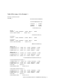
NOMENCLATURE
C
mean concentration
Cp
specific heat of air at constant pressure
C1,C2,CD,Cµ constants of turbulence model
CIN
concentration of inlet air
DELTA_
thickness of building fabric
E
east wall
EPSO_
emissivity of room surface
G
energy generation term
g
gravitational acceleration
H
room height in y direction
HC_(I)
convective heat flux for room surface I
HOBS(I)
heat flux from obstacle I
HR_(I)
radiant heat transfer flux for room surface I
HWIN_(I)
heat flux for window I
h
convective heat transfer coefficient
2
(W/m K)
I, J, K
grid point number in x, y, z direction
ICLO
thermal resistance of clothing
(m2K/W)
ICOMF
flag for thermal comfort calculations
ICON_(I)
grid coordinate of concentration source I
ICONC
flag for concentration calculations
ICOND
flag for fabric heat conduction calculation
IDR
flag for draught risk calculation
IRAD
flag for surface radiation calculation
IWIN_(I)
grid coordinate for window I
k, TK_
thermal conductivity
L
room length in x direction, or left wall
LAYER_
building fabric layer
M
metabolic rate
MAXIT
maximum number of iterations
N
north wall
NCON
number of concentration sources
NI, NJ, NK
total number of grid points in x, y, z directions
NIN
number of inlets
NP
number of monitoring points
NOBS
number of obstacles
NOUT
number of outlets
NWIN
number of windows
PMV
predicted mean vote
PPD
predicted percentage of dissatisfied
PA
water vapour pressure
p
pressure
q
heat production
R
right wall
S
south wall
Sφ
source term
t
time
T_
inside room surface temperature
TIN
inlet air temperature
TAO_
outside air temperature
UNITS
(ppm or mg/m3)
(J/kgK)
(ppm or mg/m3)
(m)
(m/s2)
(m)
(W/m2)
(W/m2)
(W/m2)
(W/m2)
(1 or 0)
(1 or 0)
(1 or 0)
(1 or 0)
(1 or 0)
(W/mK)
(m)
(W/m2)
(%)
(Pa)
(Pa)
(W/m3)
(s)
(oC)
(oC)
(oC)
TMRT
local mean radiant temperature
TOBS(I)
temperature of obstacle I
TURBIN
turbulence intensity of air at supply outlet
Uf
floor heat conduction coefficient
(W/m2K)
Ui
tensor velocity component
Ut
heat transmission coefficient for a bare floor
(W/m2K)
U,V,W
mean velocity components in x, y, z directions
VIN
inlet velocity
VAO_
outdoor air velocity
W
room width in z direction, or west wall
_WIN_
window coordinates
X(I)
position of grid I in x direction
xn
thickness of layer n
Y(J)
position of grid J in y direction
Z(K)
position of grid K in z direction
(oC)
(oC)
(m/s)
(m/s)
(m/s)
(m/s)
(m)
(m)
(m)
(m)
(m)
Greek letters
ß
ε
φ
κ
Γφ
µ, µt
ρ
σl, σt
volumetric expansion coefficient
turbulence dissipation rate
dependent variable
Karman’s constant (= 0.4187)
diffusion coefficient
laminar and turbulent viscosities of air
air density
laminar and turbulent Prandtl numbers
Subscripts
B
c
e
i
k
s
t
ε
buoyancy
concentration
effective
vector dimension
kinetic energy
shear
turbulent
kinetic energy dissipation
(1/K)
(Pa s)
(kg/m3)
1. INTRODUCTION
Air distribution systems in modern buildings require careful design to meet the increasingly stringent
demands for thermal comfort, indoor air quality and energy efficiency.
Although procedures are available for designing conventional air distribution systems, designers
have to rely on data obtained from a physical model of the proposed air distribution scheme when
dealing with a non-conventional system. Modifications to the model are then made until the desired
conditions are achieved. This procedure is very costly and time consuming. In addition, it is not
always possible to construct full scale physical models. Under such circumstances, computer based
analysis would be extremely useful in the preliminary and actual design stages.
Recently, there has been much activity in the field of Computational Fluid Dynamics (CFD) to
develop computer codes which numerically solve the differential equations that govern air
movement, heat transfer and the distribution of chemical species for internal and external flows.
Today, there are few codes which are dedicated to the built environment.
VORTEX (Ventilation Of Rooms with Turbulence and Energy eXchange) is a program which has
been specially developed to simulate the air movement, heat and concentration of species transport in
buildings. The software gives all the information that can be obtained from physical model tests, and
more, at a very low cost and within minutes or few hours, depending on the complexity of the
problem. It can also produce a full thermal comfort assessment of the indoor environment using the
ISO Standard 7730 method. The program has been under development for over eight years by
specialists in ventilation and room air movement research. A pre-processing environment has
recently been added to automate the data facility through the use of “windows-look-alike”
environment. The visualisation of the results is performed using a post-processing tool called
FLOWVIS.
2. REQUIREMENTS FOR USING VORTEX
VORTEX is a CFD code, which has been specifically developed for airflow, heat transfer and
concentration of species predictions in buildings. Unlike other general-purpose CFD codes,
scientists and engineers who have basic computing skills but not necessarily CFD experience can use
VORTEX. This manual contains examples that can be accessed by the user to gain familiarity with
the type of data required to perform a CFD simulation. However, a thorough understanding of the
problem being solved is essential to produce an “electronic model” of the building before a reliable
solution can be achieved.
VORTEX© is available for a workstation using UNIX, or for a PC using DOS 5 or higher. A
minimum of 8 Mb. RAM of available memory is required to solve small or medium size problems.
For larger problems involving extensive number of grid points, 16 Mb. or 32 Mb. RAM may be
required. An Intel 486 DX processor or a Pentium will be expected to ensure acceptable CPU run
time
3. INSTALLATION AND RUNNING
INSTALLING VORTEX.
The software can be installed by running the SETUP_310-005W.EXE program from the media
provided.
NOTE: Install the software on the root drive on your machine, (e.g. D:\ because the
installation program will automatically generate the necessary directories that are needed.
The machine also needs to be rebooted.
The software can be run using the VORTEX_310-005W icon. This will automatically run in the
directory DRIVE:\VORTEX\V310\VORT_WNT\WORKAREA
THE LOCKING DEVICE
The locking method used by VORTEX is one that generates a unique string that recognizes your
machine. You require no hardware keys, but only strings, however the user has that in order to be
provided with a unlocking string the following steps need to followed:
After installing the software on the hard disk run VORTEX using the model file SEND3. This
generates a file called SENDFILE.USR on the C:\ drive.
Send the file SENDFILE.USR to the distributor either via email or fax.
On receiving an unlocking string, file name called NTUSER31.INF, please copy this file in the
directory DRIVE:\VORTEX\V310\VORT_WNT\BIN.
if you have any problems running the software, please note any error numbers and/or messages
and contact the distributor stating these.
4. DESCRIPTION OF THE CFD MODEL
The general transport equations are the continuity equation, the Navier-Stokes (momentum)
equation, the thermal energy equation, the concentration of species equation and the two equations
for the kinetic energy and dissipation rate of the k-ε turbulence model. For incompressible flow, the
time-averaged equations are represented by:
∂( ρ φ )
∂
+
∂t
∂ x
Tansient
( ρ U
i
∂φ
∂ x
Diffusion
φ - Γ
i
Convection
) = S
φ
φ
0
(1)
i
Source
where Sφ is the source term for the variable φ (see Table 1).
To obtain a solution of equation (1) the boundary conditions for the room or building must be
specified. These are known quantities, empirical or semi-empirical expressions. Typical room
boundary conditions, which must be provided, are the velocity, temperature and the contaminant
concentration of the supply air. The air velocity, temperature and contaminant concentration at the
exit are obtained from the continuity equation, thermal energy and concentration mass balance
equations respectively. For incompressible flow as in buildings, the air density is unaffected by
pressure and therefore the pressure is a relative quantity and only pressure difference is a significant
entity.
At a solid surface a no-slip condition is imposed, i.e. zero velocity. The wall surface temperature are
either specified or computed from the heat transfer rate when a heat flux is specified at the surface.
The airflow equations are discretized and solved in a staggered 3-D Cartesian system using the
Finite Volume Method (FVM) and the well-known SIMPLE algorithm. The Hybrid Scheme (i.e.
a combination of Central Difference and Upwind Schemes) is used as the finite difference
schemes for solving the equations. To enhance the stability of the solution process underrelaxation techniques are applied to all the equations.
5. MODELLING TECHNIQUES
Input Parameters
To perform a flow simulation-using VORTEX one has to generate a problem specific data file called
model.VDB. The pre-processor generates this file after the user specifies the required variables. In
general, the user specifies the internal room dimensions, the inlet and outlet openings, the
obstructions in the room, the position of heat or contamination sources, etc. The pre-processor to suit
the room configuration then generates a computational grid. The user has the option to change the
grid setting if so desired. The heat sources at the room surfaces and those produced by certain
obstructions are specified in W/m2 of surface area. The user also specifies the inlet air velocity,
turbulence intensity, temperature and concentration.
When all the data is specified and clicking on the File icon saves the model.VDB file for the case, a
model.DAT file is automatically generated by the pre-processor and stored in the directory
DRIVE:\VORTEX\V310\VORT_NT\WORKAREA. The parameters, which are included in the
model.DAT file, are given in Table 2 and in the Examples at the end of this manual. See Section 7
for mode details.
Fire Source Data
For simulating a fire source in a room, the source is specified as a thin obstacle with a surface
temperature (TOBS(I)) ≥ 500.0oC and a heat flux (HOBS(I)) in kW/m2. The heat flux increases
with time up to a time lapse of 180 seconds using the following:
Qt+dt = 2dt/60 Qt
where Qt+dt is the heat flux at time t+dt seconds in kW/m2
Qt
is the heat flux at time t seconds in kW/m2 ; and
dt
is the time step in seconds.
The heat flux remains constant after 180 seconds.
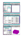
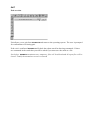
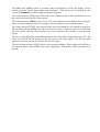
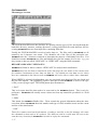
Creating *.VDB File
File Page
To create a new model.VDB file or editing an existing one, the File icon of the Vortex Setup Tool
must be opened. For a new case, the name of the case is specified in the Current File box using 8
characters maximum (without the VDB extension). The file is then saved before the Config page is
opened. For loading an existing model.VDB file, the Load box is clicked.
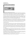
Config Page
In the Config page, Fig 2, the Active variables to be solved are specified by clicking the
corresponding box. If Comfort is required, then the metabolic rate (W/m2), the thermal resistance of
clothing (m2 K/W) and the water vapour pressure (Pa) must be specified; otherwise the default values
will be used. Similarly, if a transient solution is required, then the total time and time step must be
specified in seconds. The number of sweeps is specified in the top right hand box by either using the
arrow or typing in the value then ↵. Initially, a small number of sweeps, e.g. 2, is specified and the
results are checked to ensure that the problem has been correctly modelled. If so, then the problem
can be run for a larger number of sweeps, otherwise the necessary changes are made and the same
procedure is repeated until the correct parameters have been set. Generally, the CPU time is directly
proportional to the number of sweeps and one has to compromise between the accuracy of the
solution and the execution time. There is no easy way of determining the optimum number of
sweeps as this is a problem dependent quantity but generally, for room flow calculations, about 500
iterations are required for isothermal flow problems and about 800 iterations or more for nonisothermal flow solutions. However, the best way to ensure convergence is to check the residuals
output. It is always possible to restart the calculations for an additional number of sweeps if
convergence has not been achieved, as described in Run Page. For a case which has been previously
run and the output files are available, a restart can be performed by clicking the Restart box.
The relaxation parameters for the variables to be solved are also specified in this page; however, the
default values are adequate for the majority of cases solved. After all the data are input the Apply
box is clicked to save the values.
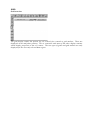
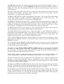
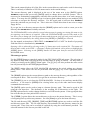
Global Page
In this page, the case name appears in the Case box (up to 8 characters) and a title is given to the case
in the Title box (up to 40 characters), see Fig 3. The room dimensions and the surface boundary
conditions are specified here too. In addition to the surface temperature, the user can also specify
surface heat fluxes (W/m2). At each room surface, there is the option of specifying a convective and
radiant flux components simultaneously. If a radiant flux is specified the emissivity of the surface
must also be specified, otherwise a default of 0.9 is used. The radiant flux will be used in the
calculation of surface-to-surface radiation exchange and the local mean radiant temperature at each
computational cell. When the convective heat flux on a surface is specified as zero, the rate of heat
transfer through the surface is calculated from the temperature difference between the thermal
boundary layer and the surface. When the heat flux on a surface is not equal to zero, the temperature
of the corresponding surface will not be used for the computation of the temperature in the boundary
layer and beyond, but instead the heat flux, together with a default surface heat transfer coefficient,
will be used for calculating the air temperature. Hence, if the heat transfer through the surface is
known to be zero (i.e. an adiabatic surface), a small value for the heat flux, say, 0.001 W/m2 instead
of 0.0 W/m2 should be used.
Clicking the Apply icon saves the data on the page.
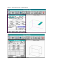
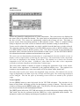
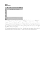
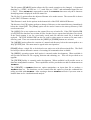
Edit Obj Page
In this page, data for the inlets, outlets, windows, obstructions and concentration sources are
specified; see Fig 4. By default there is one inlet and one outlet specified. The size and position of
each object can be changed using the arrows in X,Y,Z boxes. For the inlet the velocity
(perpendicular to the opening) must be specified together with the turbulence intensity, temperature
and concentration (ppm) if concentration is activated. For the outlet, only the size and position is
specified.
If an additional object is required then the New box is clicked to reveal a list of the objects as shown
in Fig.4. For a window, in addition to the size and position, the temperature and heat flux in W/m2 is
specified. Similarly, for an obstacle the temperature and heat flux is specified for the whole surface
of the obstacle. For an adiabatic (no heat transfer) object a small value of heat flux is specified, e.g.
0.001 W/m2, similar to the walls. After each object is entered, the Apply box is clicked and when all
the objects have been entered, the Finish box is clicked. Note up to 999 objects of each category
may be specified but the more objects are specified the larger will the computation grid be.
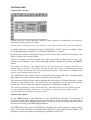
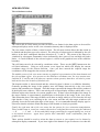
Mesh Page
The number of grids for the calculations in the X, Y and Z direction is specified here. After the user
has specified all the objects, the VORTEX pre-processor creates a default grid to fit the computation
domains (Regions), see Fig 5. However, the user can alter the number of grid points in each region
by clicking the arrows in each box. This process is repeated for the three co-ordinates. Finally, the
Finished box is clicked before leaving the page. If the data generated are required for a future run
then the user must click the Save box in the File icon, otherwise the data will not be saved.
6. RUNNING VORTEX
Run Page
After the data has been provided and saved, the model can then be run by clicking the Run icon,
which opens a new page for the main VORTEX program; see Fig. 6. As soon as this page is
opened, VORTEX waits for the user to click the Run icon to commence computing. At any time
during the execution of VORTEX (providing the number of sweeps has not been reached) the
program can be stopped and re-run as often as required. The values of the variables at the monitoring
point (Monitor Spot Value) are displayed and also plotted. In addition, the percentage change in the
variable from the previous sweep is also printed. The monitoring spot can be changed during the
execution of the program (centre of field is the default setting) by clicking the Spot Val in the Graph
icon. When the new position is typed in, it can only be affected by hitting the return key ↵.
The relaxation factor, the number of iterations, the plot frequency and the number frequency of
monitoring spot values and the residual errors can be changed at any time by clicking the Solver
icon, typing the required value and hitting ↵.
Normally, the validity of the input parameters is tested by initially executing the program for a few
iterations, e.g. 5, and the output checked to ensure that the problem has been modelled correctly.
This is done by examining the output file model.S which gives a summary of the key input
parameters such as surface temperatures, heat fluxes, position and size of the obstructions, inlet and
outlet areas, flow rate, contaminant production rate, etc. If the initial output data is acceptable the
program is then ran for a higher iteration number to obtain a converged solution. Generally, the CPU
time is directly proportional to the number of iterations and one has to compromise between the
accuracy of the solution and the execution time. There is no easy way of determining the optimum
number of iterations as this is a problem dependent quantity but generally, for room flow
calculations, about 500 iterations are required for isothermal flow problems and about 800 iterations
or more for non-isothermal flow solutions.
It is always possible to restart the calculations for an additional number of iterations if convergence
has not been achieved. When restarting, VORTEX will read all the field data produced in the
previous run as well as that in model.VDB and use them to continue the calculations.
Output Files
When the program terminates and the output files saved on disk automatically, the results can then be
visualised using FLOWVIS by clicking Post Pro in the Tasks icon. Details of carrying out the
visualisation are described under the post-processor FLOWVIS.
In additional to graphic output, the user has access to numerical data via text files. Files model.D,
model.G, model.V, model.T, model.C, model.TMRT, model.PMV, model.PPD, model.TI,
model.PD and model.AGE represent the files for room geometry (including inlets, outlets, windows
and obstructions), the computation grid in X, Y, Z co-ordinates, the velocity components U, V, W,
the temperature, the concentration, the mean radiant temperature, the Predicted Mean Vote, the
Predicted Percentage of Dissatisfied, the turbulence intensity, the Percentage of Dissatisfied due to
draught and the age of air respectively.
The file model.S contains a summary of the input data and key output parameters such as the inlet
velocity, inlet temperature, inlet concentration, volume flow rate, the Reynolds number and the
Archimedes number values for the inlet opening(s). It also contains mean values of the velocity,
temperature, concentration, PPD and the age of air (if these are computed) for each horizontal plane
in the whole field (excluding the spaces occupied by obstacles, if any). In addition, model.S gives
mean spatial values of velocity, temperature, concentration, PPD and the age of air for the occupied
zone (height of 1.8 m) and the whole space too.
File model.R contains the sum of the residuals for the velocity components (U,V,W), temperature,
kinetic energy, dissipation rate and mass flow and the values of the velocity components,
temperature, kinetic energy and dissipation rate at the monitored point (default at centre of the field).
It also gives the distribution of the variables in the field for alternate x-y planes in the field for
inspection by the user.
File model.D gives the room dimensions and the co-ordinates (W, E, S, N, L, R) of the supply and
exit openings and obstacles. File model.G gives the co-ordinates of all the grids (X(I), I = 1 to NI;
Y(J), J = 1 to NJ; Z(K), K = 1 to NK) for plotting. Note that the co-ordinates of the first and last
grid points are included in the boundary values.
Files model.ED, model.P, model.T, model.TE, model.V and model.VIS store the field grid data
for the turbulence dissipation, pressure, the air temperature, the turbulence energy, the three velocity
components and the turbulent fluid viscosity respectively. If other variables are computed, additional
output data files will also be generated. Theses files will be one or more of the following:
model.AGE, model.C, model.PD, model.PMV, model.PPD, model.TI, model.TMRT,
respectively represented the age of air, concentration of species, Predicted Dissatisfied due to
draught, Predicted Mean Vote, Predicted Percentage of Dissatisfied, the turbulence intensity and the
mean radiant temperature. These files contain the data arrays for graphical presentation or for further
processing when restarting the computation. The arrays are dumped as:
for K = 1 to NK do
for J = 1 to NJ do
for I = 1 to NI do
write variable (I,J,K)
These output files are read and used as initial values when restarting a run to reduce program running
time when a converged solution has not been reached. It should be noted that if an initial run clearly
gives a diverged solution (as indicated by the residuals in Vortex Main Program) then a restart should
not be performed but instead changes to the model.VDB data should be made before another run is
carried out. These changes may include a reduction in the values of the under relaxation factors for
the variable which is causing the divergence or a reduction in the size of source concentrations, such
as heat fluxes.
In addition to the output files described above, VORTEX also generates six other files to be
used for visualisation of the results using FLOWVIS. These are:
model.FFX,
model.FFY,
model.FFZ,
model.FHD, model.FST,
model.GEO
The latter gives the physical co-ordinates of all the inlet and outlet openings and the obstructions and
the corresponding colour code for plotting these using FLOWVIS. The user if desires can change
the colour codes.
7. OTHER INPUT DATA FILES
File MODEL.DAT
When the VORTEX pre-processor is used to generate a grid, it divides each region into a uniformly
spaced grid. However, the user can generate his/her own computational grid for each region in the
field by generating a model.DAT file using an editor in the same format as required by VORTEX.
This offers the user the flexibility for specifying his/her own grid geometry, e.g. a non-uniform grid
for each or some of the regions. The format of the model.DAT file is given in Table 2 and the
*.DAT files for the Examples.
After generating a specific Model.DAT file and saved in the directory C:\VORTEX|WORKAREA
this can be run using the following steps:
(I) Open an existing *.VDB file using the Vortex Post-rocessor and click the Run icon.
(ii) Go to File icon in Vortex Main Program and select open.
(iii) Type the name of the file generated, e.g. user.DAT (without the .DAT extension) and
press ↵.
(iv) Click the Open box and the user.DAT file will be run normally.
and
File FABRIC.DAT
If the internal room surface temperatures or heat fluxes are not known VORTEX has the option of
generating the required boundary conditions using external weather data and building fabric data.
This is done assuming steady-state conduction through the fabric, i.e. heat storage is not considered.
At present, the input required for defining the fabric data is via a separate input file called
FABRIC.DAT. The structure of this data file is described below.
If the fabric heat loss/gain is to be taken into account, data are required for the wind velocity, VAO-,
temperature, TAO-, emissivity of exterior wall surface, EPSO-, the number of structural
components, LAYER-, thickness, DELTA-, and thermal conductivity, TK-, of each component, for
each of the walls, roof and floor. The data are set in a separate file called FABRIC.DAT in the
following format:
VAOW VAOE
TAOW TAOE
EPSOW EPSOE
VAOS VAON VAOL VAOR
TAOS TAON TAOL TAOR
EPSOS EPSON EPSOL EPSOR
LAYERW
DELTAW(I) (I=1, LAYERW)
TKW(I) (I=1, LAYERW)
LAYERE
DELTAE(I) (I=1, LAYERE)
TKE(I) (I=1, LAYERE)
LAYERS
DELTAS(I) (I=1, LAYERS)
TKS(I) (I=1, LAYERS)
LAYERN
DELTAN(I) (I=1, LAYERN)
TKN(I) (I=1, LAYERN)
LAYERL
DELTAL(I) (I=1, LAYERL)
TKL(I) (I=1, LAYERL)
LAYERR
DELTAR(I) (I=1, LAYERR)
TKR(I) (I=1, LAYERR)
where the last characters of the parameters, W, E, S, N, L, R, are the west, east, south, north, left and
right surfaces respectively. The thickness or thermal conductivity of each component of a wall must
also be set in the same line.
In the case of a known thermal resistance, e.g. air cavity, the thickness of the layer (DELTA-) is
taken as 1 m and the thermal conductivity (TK-) is taken as the reciprocal of this resistance.
The default data for the above variables are as follows:
VAO- = VIN
TAO- = TIN
EPSO- = 0.9
LAYER- = 1
DELTA- = 0.22 m
TK= 0.84 W/mK
for the west, east, north, left and right surfaces.
For an intermediate floor or ceiling the fabric heat loss/gain is calculated in the same way as the
walls. For the ground floor the equation below applies:
1
1
--- = -- +
Uf Ut
xn
1
- -kn hi
Σ ---
(2)
where
Uf = floor heat conduction coefficient excluding internal surface resistance (W/m2K)
Ut=
tabulated value of the overall heat transmission coefficient for a bare ground floor (W/m2K)
xn =
thickness of layers above the floor, e.g. insulation carpet, etc. (m)
kn =
thermal conductivity of each layer (W/mK)
hi =
internal surface heat transfer coefficient (dependent on direction of heat flow) (W/m2K).
The program calculates a default heat transfer coefficient for a ground floor using:
VAOS = 10000.0 (no exterior surface film resistance)
TAOS = TIN
EPSOS = 0.0
LAYERS = 1
TKS / DELTAS = 2.73 W/m2K (carpet and fibrous pad)
However, a more accurate value of the heat transfer coefficient of the floor can be calculated using
Equation (2) and this can be used for overwriting the default value.
If all the default values are applicable for the problem being investigated, FABRIC.DAT is not
required. If the values for outdoor velocity and temperature are different from the default data while
those for the fabric are the same as the default data, input the data for the velocity and temperature
only. Thus, the input data can be simplified to:
VAOW
TAOW
VAOE
TAOE
VAOS
TAOS
VAON
TAON
VAOL
TAOL
VAOR
TAOR
If the emissivity of exterior wall surfaces needs to be specified as well as the velocity and
temperature, the input data will become:
VAOW VAOE
TAOW TAOE
EPSOW EPSOE
VAOS VAON VAOL VAOR
TAOS TAON TAOL TAOR
EPSOS EPSON EPSOL EPSOR
8. EXAMPLES
The following examples illustrate the use of VORTEX. In the first example, only the velocity and
temperature distributions are required. The second example shows a more comprehensive analysis of
variables, including thermal comfort analysis. The third example represents a buoyancy-driven,
naturally ventilated enclosure.
Example 1
This example illustrates the use of the program for predicting the environment in an office which is
cooled by supplying air from a wall at high level and extracting air from the ceiling.
The air is supply rate is 0.096 m3/s at a speed of 2.0 m/s and temperature 12oC to the room, which
has the dimensions given below, through a diffuser situated on the middle of the west wall close to
the ceiling:
LENGTH = 4.0 m
HEIGHT = 2.7 m
WIDTH = 3.0 m
The effective dimensions of the diffuser are 1.2 m long and 0.04 m wide. The air is extracted
through a 0.4m x 0.4m ceiling opening close to the the curtain wall (east wall).
The inside temperature of each wall is assumed to be 25oC. There is heat generation on the floor at a
rate of 50 W/m2. A window, 1.6 m wide and 1.75 m high, is situated on the east wall, 0.55 m above
the floor. The temperature of the window is assumed to be 28oC. There are two obstacles in the
room, one table (at a temperature of 24oC) and one occupant (standing position) with an assumed
surface temperature of 33oC and a metabolic heat production rate of 50 W/m2.
The input data for this case is given in Table 3 as file examp_1.DAT. The of regions are
automatically selected by the program, depending on the number and position of the objects in the
room. A default (minimum) value for the number of grids for each region is specified but the user
has the option to change the number of grid points in each region. The grid chosen for this example
is 31* 26 *32. The finer the grid the more accurate the solution will be but this is at the expense of a
longer run time. Generally, if the grid size in each direction is doubled it will take 8 times longer to
run the problem for the same number of iterations.
A theoretical investigation has been carried out to optimise the distance of the nearest grid point from
a solid surface and was found that this distance should be set to about 0.01 m to achieve a region
which is most appropriate for the application of the turbulent flow wall functions used in VORTEX.
The computation results for this case are presented graphically in Figures 7 and 8 as velocity vectors
and temperature contours for two planes. One vertical plane through the supply diffuser and the
other one is a horizontal plane. The values of the velocity components, temperature, etc. for each
grid point can be found in file examp_1.R and a summary result of the output in File examp_1.S
(see Table 4).
Example 2
This is a heating example for the same office room described in Example 1 with a square diffuser at
the centre of the ceiling discharging the air radially. The supply air flow rate is 0.09 m3/s. The size
of the square diffuser is 0.6 m x 0.6 m x 0.1 m effective slot width. The supply air temperature is
30oC. This room is on the ground floor of a building which has three external walls, one internal
wall (west wall) and a ceiling adjoining the floor of the next level. The internal temperatures of the
ceiling and the west wall are known to be both 21oC, whereas the internal temperatures of the floor
and the other three walls are not known. However, the outdoor design temperature is given as 1oC
and the design wind speed is 3.4 m/s. The single-glazed window has an internal temperature of 10oC
which is calculated from the U-value, the outdoor temperature and the estimated room temperature of
24oC. There are also heat losses from the curtain wall of 20 W/m2 and from the floor of 25 W/m2.
The room is constructed using standard building materials, i.e. the default values of fabric properties
given in file FABRIC.DAT are assumed to apply here. In addition to calculating the heat loss
through the external room surfaces to determine their internal surface temperature, this example also
analyses the thermal comfort in the room.
The file examp_2.DAT for this example is given in Table 5. Only minor changes have been made to
the file for Example 1 in Table 3. The Comfort and Conduction boxes are both selected for the
computation of thermal comfort and conduction heat transfer through the external surfaces. The
opening area (0.3 x 0.3 ) = 0.09 m2. For the give flow rate of 0.09 m3/s the supply air velocity is 1
m/s at the inlet (duct) position. However, this is not the supply velocity to the room as the diffuser
will diffuse the air in a radial direction over the ceiling.
To represent this effect a thin baffle plate (obstacle) 0.6 m x 0.6 m is positioned 0.1m below the inlet
opening to provide a radial diffusion of the supply air and effectively representing the action of the
diffuser. This is of course a simplification to the complex aerodynamics of a ceiling diffuser but if
the gap between the baffle and the ceiling is set to produce the same supply velocity as the actual
diffuser this approximation should produce reliable results.
The setting of room surface temperature is no longer critical for this example because the true values
are calculated using the heat conduction equations through the fabric. Therefore, only approximate
values for the internal surface temperatures need to be specified.
File FABRIC.DAT is created to input the outdoor environmental conditions for the calculation of
fabric heat transfer with the following data:
3.4
1.0
3.4 10000.0 0.0 0.0
1.0
10.0 24.0 24.0
3.4
1.0
The results of the computation are shown plotted in Figures 9 to 11 for velocity, air temperature,
mean radiant temperature and predicted percentage of dissatisfied. Table 6 shows the summary
output data for the problem in the form of file examp_2.S
Example 3
This example deals with a large enclosure (e.g. atrium) which is naturally ventilated by an open door
and two top outlets on either side of the structure. The air enters through the door and rises up by
the buoyancy resulting from the heat flux on the roof and the floor (e.g. solar gain). It is assumed
that the other four surfaces are adiabatic. There are two platforms just below the outlets running
across the whole building and 2 m wide and 0.15m thick.
The internal dimensions of the enclosure are:
LENGTH = 12.0 m
HEIGHT = 10.0 m
WIDTH = 8.0 m
The outdoor air temperature is assumed to be 22.0oC and the heat fluxes on the roof and the floor are
50 and 25 W/m2 respectively. The door is 2.0 m high and 1.5 m wide and is located on the west
wall. The two outlets are 0.8 m high and 1.5 m wide each and are located at the top of the west and
east walls. It is also assumed that there are 50 people occupying the building each producing 4.7
ml/s of CO2.
To activate the calculation for buoyancy the inlet velocity must be specified as 0.01 m/s but the true
inlet velocity will be calculated by the program and updated during each iteration. The heat fluxes
on the roof and floor are specified and an estimate is made of the temperature for these two surfaces.
However, these temperatures will not be used in the calculations as the heat flux has a precedent over
surface temperatures. To represent an adiabatic wall, a very small heat flux (e.g. 0.001) is specified
for the wall and an approximate wall surface temperature is specified. This is the case for the four
adiabatic walls in this example.
The 50 CO2 concentration sources are spread over two regions to include 50 node points and the
emission for each node is specified in ml/s. These are point sources which are determined by the
number of grid points selected for this region in each direction. For each of the two regions, only one
grid point is selected for the y direction, 5 grid points are selected in each of the x and z direction
giving a total number of source point for the region of 1*5*5 = 25. The total CO2 emission is 0.235
l/s. examp_3 .DAT for this example is given in Table 7.
The results of the computation for velocity, temperature and CO2 concentration in ppm are plotted in
Figures 12 and 13 for two planes across the building. Table 8 shows a summary output.
Table 1. Source terms of the flow equations
Equation
Continuity
φ
1
Γφ
0
U-momentum
U
µe
V-momentum
V
µe
W-momentum
W
µe
Temperature
T
Γe
Concentration
C
Γc
Sc
Kinetic energy
k
Γk
Dissipation rate ε
Γε
Gs - CD ρ ε + GB
ε
ε2
C1 -- (Gs + GB) - C2 ρ -k
k
Notes: µe = µ + µt
Γe = µt/σt + µ/σl
Γk = µe/σk
Sφ
0
∂p ∂ ∂U ∂ ∂V ∂ ∂W 2 ∂
- --+ -- (µe--) + -- (µe--) + -- (µe--)- - -- (ρk)
∂x ∂x ∂x ∂y ∂x ∂z ∂x 3 ∂x
∂p ∂ ∂U ∂ ∂V ∂ ∂W 2 ∂
- -- + -- (µe--) + -- (µe--) + -- (µe--) - - -- (ρk)
∂y ∂x ∂y ∂y ∂y ∂z ∂y 3 ∂y
- g (ρ - ρo)
∂p ∂ ∂U ∂ ∂V ∂ ∂W 2 ∂
- -- + -- (µe--) + -- (µe--) + -- (µe--) - -- -- (ρk)
∂z ∂x ∂z ∂y ∂z ∂z ∂z 3 ∂y
q / Cp
σε = κ2/ /(C2 - C1)Cµ1/2
µt = Cµρk2/ε
Γc = µt/σc + µ/σl
Γε = µe/σε
Kinetic energy generation by shear
∂U2 ∂V ∂W2 ∂U ∂V2 ∂U ∂W2 ∂V ∂W2
Gs = µt {2 [(---) + (---) + (---)] + (--+---) + (-- + ---) + (-- + ---)}
∂x ∂y
∂z
∂y ∂x ∂z ∂x
∂z ∂y
Kinetic energy generation by buoyancy
µt ∂T
GB = ßg -----σt ∂y
Empirical constants in the equations
Cµ
0.09
CD
1.0
C1
1.44
C2
1.92
σc
0.9
σk
1.0
σt
0.9
Table 2. Structure of MODEL.DAT (comments in lower case)
Variable List
Summary of Variable List
ICONC, ICOMF, IDRA, IRADI,
ICOND,IAGE
L, H, W
NI, NJ, NK
Control flags for concentration, comfort, draught,
Radiation, conduction and age
Length, Height & Width
Maximum grid number in x (length), y (Height),z(Width)
Directions
Grid and corresponding coordinate in x direction (I=1 to NI)
Grid and corresponding coordinate in y direction (J=1 to NJ)
Grid and corresponding coordinate in z direction(K=1to NK)
Number of air supply openings
Coordinates of supply opening I (I=1 to NIN)
I, X(I)
J, Y(J)
K, Z(K)
NIN
IINW(I), IINE(I), JINS(I), JINN(I),
KINL(I), KINR(I)
NOUT
IOUTW(I), IOUTE(I), JOUTS(I),
JOUTN(I), KOUTL(I), KOUTR(I)
NWIN
IWINW(I), IWINE(I), JWINS(I),
JWINN(I),KWINL(I), KWINR(I),
TWIN(I), HWIN(I)
NOBS
IOBSW(I), IOBSE(I), JOBSS(I),
JOBSN(I), KOBSL(I), KOBSR(I),
TOBS(I), HOBS(I)
NCON
ICONW(I), ICONE(I), JCONS(I),
JCONN(I), KCONL(I), KCONR(I),
C(I)
TW, TE, TS, TN, TL, TR
HCW, HCE, HCS, HCN, HCL, HCR
HRW, HRE, HRS, HRN, HRL, HRR
EPSW, EPSE, EPSS, EPSN, EPSL,
EPSR
UIN, VIN, WIN, DC, TURBIN, TIN,
CIN
MAXIT
URFU, URFV, URFW, URFP,
URFK, URFE, URFVIS, URFT,
URFC, URFG
M, ICLO, PA
NP
X(I), Y(I), Z(I)
Number of air exits
Coordinates of exit opening I (I=1 to NOUT)
Number of windows
Coordinates, temperature and heat flux (W/m2)of window I
(I=1 to NWIN)
Number of obstacles
Coordinates, temperature and heat production (W/m2) of
obstacle I (I=1 to NOBS)
Number of concentration sources
Coordinates and generation rate (ml/s or mg/s) of
concentration source I (I=1 to NCONC)
Wall surface temperatures
Convective heat fluxes on room surfaces
Radiant heat fluxes on surfaces
Emissivity of interior wall surfaces
U, V and W Velocity, Discharge coefficient, turbulence
intensity, temperature and concentration of supply air
Maximum number of iterations
Under relaxation factors
Metabolic rate, thermal resistance of clothing and partial
water vapour pressure
Number of points for output data
Coordinates of point I (I=1 to NP)
Table 3. File examp_1.DAT for Example 1
Wall Supply
EXAMP_1
0 0 0 0 0
4.00000e+000 2.70000e+000 3.00000e+000
31 25 32
1 -1.000000e-002
2 1.000000e-002
3 1.466667e-001
4 4.000000e-001
5 6.533333e-001
6 7.900000e-001
7 8.100000e-001
8 9.800000e-001
9 1.300000e+000
10 1.620000e+000
11 1.790000e+000
12 1.810000e+000
13 1.860000e+000
14 1.940000e+000
15 1.990000e+000
16 2.010000e+000
17 2.135000e+000
18 2.365000e+000
19 2.490000e+000
20 2.510000e+000
21 2.680000e+000
22 3.000000e+000
23 3.319999e+000
24 3.489999e+000
25 3.509999e+000
26 3.699999e+000
27 3.889999e+000
28 3.909999e+000
29 3.949999e+000
30 3.990000e+000
31 4.010000e+000
1 -1.000000e-002
2 1.000000e-002
3 1.475000e-001
4 4.024999e-001
5 5.399998e-001
6 5.599998e-001
7 5.999999e-001
8 6.400000e-001
9 6.600000e-001
10 7.000000e-001
11 7.400000e-001
12 7.600000e-001
13 1.010000e+000
14 1.490000e+000
15 1.740000e+000
16 1.760000e+000
17 1.897500e+000
18 2.152500e+000
19 2.290000e+000
20 2.310000e+000
21
22
23
24
25
2.480000e+000
2.650000e+000
2.670000e+000
2.690000e+000
2.710000e+000
1 -1.000000e-002
2 1.000000e-002
3 1.850000e-001
4 5.150000e-001
5 6.900001e-001
6 7.100000e-001
7 8.000001e-001
8 8.900001e-001
9 9.100001e-001
10 1.018750e+000
11 1.127500e+000
12 1.147500e+000
13 1.218750e+000
14 1.290000e+000
15 1.310000e+000
16 1.468750e+000
17 1.627500e+000
18 1.647500e+000
19 1.668750e+000
20 1.690000e+000
21 1.710000e+000
22 1.810000e+000
23 1.990000e+000
24 2.090000e+000
25 2.110000e+000
26 2.200000e+000
27 2.290001e+000
28 2.310001e+000
29 2.485001e+000
30 2.815000e+000
31 2.990000e+000
32 3.010000e+000
1
1 1 23 24 9 24
1
25 27 25 25 15 20
1
31 31 6 19 6 27 2.80000e+001 0.00000e+000
2
7 11 9 11 9 24 2.40000e+001 0.00000e+000
16 19 2 15 12 17 3.30000e+001 5.00000e+001
0
2.50000e+001
0.00000e+000
2.50000e+001
0.00000e+000
2.50000e+001
5.00000e+001
2.00000e+000 4.99997e-002 1.20000e+001
900
2.50000e+001 2.50000e+001
0.00000e+000 0.00000e+000
2.50000e+001
0.00000e+000
5.00000e-001
5.00000e-001
5.00000e-001
8.00000e-001
5.00000e-001
5.00000e-001
8.00000e-001
5.00000e-001
0
0
: TRANSIENT -> TOTAL_TIME, STEP_SIZE
0
: RESTART -> CONC, COMFORT, DRAUGHT, RAD,
CONDUCT, AGE
Table 4 File examp_1.S for Example 1
Wall Supply
EXAMP_1
* ROOM AIR MOVEMENT *
ROOM DIMENSIONS (m)
LENGTH
WIDTH
HEIGHT
=
=
=
4.0000
3.0000
2.7000
FLUID INLET (m)
INLET 1
WIDTH = 1.2000 , HEIGHT = 0.0400 , AREA = 0.0480
TOTAL INLET AREA =
0.0480 m**2
FLUID OUTLET (m)
OUTLET 1
WIDTH = 0.4000 , HEIGHT = 0.4000 , AREA = 0.1600
TOTAL OUTLET AREA =
0.1600 m**2
OBSTACLE SIZE (m)
OBSTACLE 1
X-DIRECTION: X1 = 0.8000 , X2 = 1.8000 , LENGTH = 1.0000
Y-DIRECTION: Y1 = 0.6500 , Y2 = 0.7500 , HEIGHT = 0.1000
Z-DIRECTION: Z1 = 0.9000 , Z2 = 2.1000 , WIDTH = 1.2000
OBSTACLE 2
X-DIRECTION: X1 = 2.0000 , X2 = 2.5000 , LENGTH = 0.5000
Y-DIRECTION: Y1 = 0.0000 , Y2 = 1.7500 , HEIGHT = 1.7500
Z-DIRECTION: Z1 = 1.1375 , Z2 = 1.6375 , WIDTH = 0.5000
WINDOWS (m)
WINDOW 1
WIDTH = 1.6000 , HEIGHT = 1.7500 , AREA = 2.8000
TOTAL AREA OF WINDOWS =
2.8000 m**2
INLET FLUID PROPERTIES
VELOCITY
=
2.000E+0 m/s
TURBULENCE INTENSITY =
5.000E-2
TEMPERATURE
=
1.200E+1
DENSITY
=
1.232E+0
LAMINAR VISCOSITY
=
1.771E-5
AIR FLOW RATE
=
9.600E-2
REYNOLDS NUMBER
=
5.567E+3
PRANDTL NUMBER
=
7.050E-1
deg.C
kg/m**3
Pa s
m**3/s
INITIAL INSIDE SURFACE TEMPERATURE (deg. C)
WEST WALL
EAST WALL
FLOOR
CEILING
LEFT WALL
RIGHT WALL
WINDOW 1
OBSTACLE 1
OBSTACLE 2
=
=
=
=
=
=
=
=
=
25.0000
25.0000
25.0000
25.0000
25.0000
25.0000
28.0000
24.0000
33.0000
CONVECTIVE HEAT FLUX ON SURFACES (W/m**2)
WEST WALL
EAST WALL
FLOOR
CEILING
LEFT WALL
RIGHT WALL
WINDOW 1
OBSTACLE 1
OBSTACLE 2
= 0.0000
= 0.0000
= 50.0000
= 0.0000
= 0.0000
= 0.0000
= 0.0000
= 0.0000
= 50.0000
ARCHIMEDES NUMBER =
0.337E-2
MEAN VALUES AT DIFFERENT HEIGHT LEVELS
GRID HEIGHT
(m)
VELOCITY
(m/s)
TEMPERATURE
(deg.C)
2
3
4
5
6
7
8
9
10
11
12
13
14
15
16
17
18
19
20
0.2643
0.2261
0.1891
0.1743
0.1713
0.1666
0.1633
0.1690
0.1633
0.1582
0.1455
0.1241
0.1296
0.1368
0.1352
0.1495
0.1765
0.1929
0.1981
25.2267
23.7670
23.7162
23.7878
23.8006
23.8202
23.8364
23.7377
23.7459
23.7498
23.7483
23.7846
23.8584
23.8906
23.9483
23.9587
23.8478
23.6041
23.5301
0.0100
0.1475
0.4025
0.5400
0.5600
0.6000
0.6400
0.6600
0.7000
0.7400
0.7600
1.0100
1.4900
1.7400
1.7600
1.8975
2.1525
2.2900
2.3100
21
22
23
24
2.4800
2.6500
2.6700
2.6900
0.2197
0.3233
0.4580
0.4647
23.3750
22.8203
22.3344
22.4381
MEAN VALUES IN THE OCCUPIED ZONE
(from floor to height 1.8 m)
AIR VELOCITY
AIR TEMPERATURE
=
0.2643 m/s
= 25.2267 deg.C
MEAN VALUES IN THE SPACE
AIR VELOCITY
AIR TEMPERATURE
= 0.1762 m/s
= 23.7598
Table 5 File examp_2.DAT for Example 2
Ceiling supply
EXAMP_2
0 1 0 0 1
4.00000e+000 2.70000e+000 3.00000e+000
38 34 37
1 -1.000000e-002
2 1.000000e-002
3 1.466667e-001
4 4.000000e-001
5 6.533334e-001
6 7.900001e-001
7 8.100001e-001
8 9.633334e-001
9 1.250000e+000
10 1.536667e+000
11 1.690000e+000
12 1.710000e+000
13 1.750000e+000
14 1.790000e+000
15 1.810000e+000
16 1.825000e+000
17 1.840000e+000
18 1.860000e+000
19 1.925000e+000
20 1.990000e+000
21 2.010000e+000
22 2.075000e+000
23 2.140000e+000
24 2.160000e+000
25 2.225000e+000
26 2.290000e+000
27 2.310000e+000
28 2.346667e+000
29 2.400000e+000
30 2.453334e+000
31 2.490000e+000
32 2.510000e+000
33 2.702500e+000
34 3.067500e+000
35 3.432500e+000
36 3.797500e+000
37 3.990000e+000
38 4.010000e+000
1 -1.000000e-002
2 1.000000e-002
3 1.099999e-001
4 2.899998e-001
5 3.899998e-001
6 4.099998e-001
7 4.749999e-001
8 5.400000e-001
9 5.600000e-001
10 6.000000e-001
11 6.400000e-001
12 6.600000e-001
13 7.000000e-001
14
15
16
17
18
19
20
21
22
23
24
25
26
27
28
29
30
31
32
33
34
7.400000e-001
7.600000e-001
9.300000e-001
1.250000e+000
1.570000e+000
1.740000e+000
1.760000e+000
1.897500e+000
2.152500e+000
2.290000e+000
2.310000e+000
2.400000e+000
2.490000e+000
2.510000e+000
2.550000e+000
2.590000e+000
2.610000e+000
2.635000e+000
2.665000e+000
2.690000e+000
2.710000e+000
1 -1.000000e-002
2 1.000000e-002
3 1.850000e-001
4 5.150000e-001
5 6.900001e-001
6 7.100000e-001
7 8.000001e-001
8 8.900001e-001
9 9.100001e-001
10 1.050000e+000
11 1.190000e+000
12 1.210000e+000
13 1.225000e+000
14 1.240000e+000
15 1.260000e+000
16 1.300000e+000
17 1.340000e+000
18 1.360000e+000
19 1.500000e+000
20 1.640000e+000
21 1.660000e+000
22 1.700000e+000
23 1.740000e+000
24 1.760000e+000
25 1.775000e+000
26 1.790000e+000
27 1.810000e+000
28 1.950000e+000
29 2.090000e+000
30 2.110000e+000
31 2.200001e+000
32 2.290001e+000
33 2.310001e+000
34 2.485001e+000
35 2.815000e+000
36 2.990000e+000
37 3.010000e+000
1
18 23 34 34 18 20
1
1 1 2 5 18 23
1
38 38 9 23 6 32 1.00000e+001 0.00000e+000
3
12 26 27 29 12 26 2.80000e+001 0.00000e+000
7 14 12 14 9 29 2.40000e+001 1.00000e-002
21 31 2 19 15 23 3.30000e+001 5.00000e+001
0
2.10000e+001
0.00000e+000
2.10000e+001
-2.00000e+001
2.10000e+001 2.10000e+001 2.10000e+001
2.10000e+001
-2.50000e+001 0.00000e+000 0.00000e+000 0.00000e+000
1.00000e+000 4.99997e-002 2.80000e+001
800
5.00000e-001
5.00000e-001
5.00000e-001
8.00000e-001
5.00000e-001
5.00000e-001
8.00000e-001
5.00000e-001
7.00000e+001 1.10000e-001 1.50000e+003
0
0
: TRANSIENT -> TOTAL_TIME, STEP_SIZE
0
: RESTART -> CONC, COMFORT, DRAUGHT, RAD,CONDUCT, AGE
Table 6 File examp_2.S for Example 2
Ceiling supply
EXAMP_2
* ROOM AIR MOVEMENT *
ROOM DIMENSIONS (m)
LENGTH
WIDTH
HEIGHT
=
=
=
4.0000
3.0000
2.7000
FLUID INLET (m)
INLET 1
WIDTH = 0.3000 , HEIGHT = 0.3000 , AREA =
TOTAL INLET AREA =
0.0900 m**2
0.0900
FLUID OUTLET (m)
OUTLET 1
WIDTH = 0.4000 , HEIGHT = 0.4000 , AREA =
TOTAL OUTLET AREA =
0.1600 m**2
0.1600
OBSTACLE SIZE (m)
OBSTACLE 1
X-DIRECTION: X1 = 1.7000 , X2 = 2.3000 , LENGTH = 0.6000
Y-DIRECTION: Y1 = 2.5000 , Y2 = 2.6000 , HEIGHT = 0.1000
Z-DIRECTION: Z1 = 1.2000 , Z2 = 1.8000 , WIDTH = 0.6000
OBSTACLE 2
X-DIRECTION: X1 = 0.8000 , X2 = 1.8000 , LENGTH = 1.0000
Y-DIRECTION: Y1 = 0.6500 , Y2 = 0.7500 , HEIGHT = 0.1000
Z-DIRECTION: Z1 = 0.9000 , Z2 = 2.1000 , WIDTH = 1.2000
OBSTACLE 3
X-DIRECTION: X1 = 2.0000 , X2 = 2.5000 , LENGTH = 0.5000
Y-DIRECTION: Y1 = 0.0000 , Y2 = 1.7500 , HEIGHT = 1.7500
Z-DIRECTION: Z1 = 1.2500 , Z2 = 1.7500 , WIDTH = 0.5000
WINDOWS (m)
WINDOW 1
WIDTH = 1.6000 , HEIGHT = 1.7500 , AREA = 2.8000
TOTAL AREA OF WINDOWS =
2.8000 m**2
INLET FLUID PROPERTIES
VELOCITY
TURBULENCE INTENSITY
TEMPERATURE
DENSITY
LAMINAR VISCOSITY
AIR FLOW RATE
REYNOLDS NUMBER
PRANDTL NUMBER
=
=
=
=
=
=
=
=
1.000E+0
5.000E-2
2.800E+1
1.167E+0
1.848E-5
9.000E-2
1.894E+4
7.050E-1
m/s
deg.C
kg/m**3
Pa s
m**3/s
INITIAL INSIDE SURFACE TEMPERATURE (deg. C)
WEST WALL
EAST WALL
FLOOR
CEILING
LEFT WALL
=
=
=
=
=
21.0000
21.0000
21.0000
21.0000
21.0000
RIGHT WALL
WINDOW 1
OBSTACLE 1
OBSTACLE 2
OBSTACLE 3
=
=
=
=
=
21.0000
10.0000
28.0000
24.0000
33.0000
CONVECTIVE HEAT FLUX ON SURFACES (W/m**2)
WEST WALL
EAST WALL
FLOOR
CEILING
LEFT WALL
RIGHT WALL
WINDOW 1
OBSTACLE 1
OBSTACLE 2
OBSTACLE 3
ARCHIMEDES NUMBER =
= 0.0000
= -20.0000
= -25.0000
= 0.0000
= 0.0000
= 0.0000
= 0.0000
= 0.0000
= 0.0100
= 50.0000
0.588E-1
MEAN VALUES AT DIFFERENT HEIGHT LEVELS
GRID
HEIGHT
(m)
VELOCITY
(m/s)
TEMPERATURE
(deg.C)
PPD
(%)
2
3
4
5
6
7
8
9
10
11
12
13
14
15
16
17
18
19
20
21
22
23
24
25
26
27
28
29
30
31
32
33
0.0100
0.1100
0.2900
0.3900
0.4100
0.4750
0.5400
0.5600
0.6000
0.6400
0.6600
0.7000
0.7400
0.7600
0.9300
1.2500
1.5700
1.7400
1.7600
1.8975
2.1525
2.2900
2.3100
2.4000
2.4900
2.5100
2.5500
2.5900
2.6100
2.6350
2.6650
2.6900
0.0411
0.0390
0.0361
0.0334
0.0320
0.0294
0.0275
0.0269
0.0260
0.0250
0.0237
0.0227
0.0222
0.0216
0.0177
0.0159
0.0171
0.0165
0.0165
0.0169
0.0230
0.0299
0.0318
0.0335
0.0335
0.0362
0.0500
0.0834
0.1514
0.1647
0.1691
0.1628
18.8165
20.1507
20.7998
21.0946
21.1576
21.3260
21.4893
21.5429
21.6395
21.7364
21.8538
21.9597
22.0629
22.1702
22.5210
23.1077
23.6641
23.9666
24.0508
24.2727
24.7394
25.0394
25.0988
25.2977
25.5273
25.6149
25.7635
25.9620
26.1898
26.3393
26.4723
26.5418
44.2161
28.6887
23.9167
21.4450
20.7442
19.6995
18.5629
18.2330
17.7423
17.1284
16.6565
16.1703
15.5793
15.1046
13.5197
11.0114
8.9385
7.8009
7.4471
6.9226
6.0424
5.6205
5.3816
5.3065
5.2744
5.2921
5.3485
5.3707
5.3750
5.3890
5.4389
7.9241
MEAN VALUES IN THE OCCUPIED ZONE
(from floor to height 1.8 m)
AIR VELOCITY
AIR TEMPERATURE
PREDICTED MEAN VOTE
PREDICTED PERCENTAGE OF DISSATISFIED
= 0.0411 m/s
= 18.8165 deg.C
= -1.4005
= 44.2161 %
MEAN VALUES IN THE SPACE
AIR VELOCITY
AIR TEMPERATURE
MEAN RADIANT TEMPERATURE
PREDICTED MEAN VOTE
PREDICTED PERCENTAGE OF DISSATISFIED
=
=
=
=
=
0.0303 m/s
23.1789 deg.C
18.9988 deg.C
-0.4815
12.7640 %
TEMPERATURE AT THE EXIT
VENTILATION EFFICIENCY
PREDICTED PERCENTAGE OF DISSATISFIED
= 0.2198E+2 deg.C
= 0.6552E+2 %
= 0.4422E+2 %
Table 7 File examp_3.DAT for Example 3
Naturally Ventilated Atrium
Examp_3
1 0 0 0 0
1.20000e+001 1.00000e+001 8.00000e+000
27 29 20
1 -1.000000e-002
2 1.000000e-002
3 3.466667e-001
4 1.000000e+000
5 1.653334e+000
6 1.990000e+000
7 2.010000e+000
8 2.430000e+000
9 3.250000e+000
10 4.070000e+000
11 4.490000e+000
12 4.510000e+000
13 4.912500e+000
14 5.697500e+000
15 6.482500e+000
16 7.267500e+000
17 8.052500e+000
18 8.837500e+000
19 9.240000e+000
20 9.260000e+000
21 9.625000e+000
22 9.990000e+000
23 1.001000e+001
24 1.051000e+001
25 1.149000e+001
26 1.199000e+001
27 1.201000e+001
1 -1.000000e-002
2 1.000000e-002
3 2.025000e-001
4 5.675000e-001
5 9.325000e-001
6 1.297500e+000
7 1.490000e+000
8 1.525000e+000
9 1.560000e+000
10 1.672500e+000
11 1.877500e+000
12 1.990000e+000
13 2.010000e+000
14 2.520714e+000
15 3.522143e+000
16 4.523571e+000
17 5.525000e+000
18 6.526429e+000
19 7.527857e+000
20 8.529285e+000
21 9.040000e+000
22 9.060000e+000
23 9.125000e+000
24 9.189999e+000
25 9.209999e+000
26 9.409999e+000
27 9.789999e+000
28 9.989999e+000
29 1.001000e+001
1 -1.000000e-002
2 1.000000e-002
3 3.750000e-001
4 7.400000e-001
5 7.600000e-001
6 1.385000e+000
7 2.615000e+000
8 3.240000e+000
9 3.260000e+000
10 3.635000e+000
11 4.365000e+000
12 4.740000e+000
13 4.760000e+000
14 5.385000e+000
15 6.615000e+000
16 7.240000e+000
17 7.260000e+000
18 7.625000e+000
19 7.990000e+000
20 8.010000e+000
1
1 1 2 12 9 12
2
1 1 25 28 9 12
27 27 25 28 9 12
0
2
2 6 22 24 2 19 2.50000e+001 1.00000e-003
23 26 22 24 2 19 2.50000e+001 1.00000e-003
2
12 19 8 8 5 8 4.70000e+000
12 19 8 8 13 16 4.70000e+000
2.50000e+001 2.50000e+001 2.50000e+001 2.50000e+001 2.50000e+001 2.50000e+001
1.00000e-003 1.00000e-003 2.50000e+001 5.00000e+001 1.00000e-003 1.00000e-003
1.00000e-002 5.00000e-002 2.20000e+001 3.50000e+002
1200
5.00000e-001
5.00000e-001
5.00000e-001
8.00000e-001
5.00000e-001
5.00000e-001
8.00000e-001
5.00000e-001
8.00000e-001
0
0
: TRANSIENT -> TOTAL_TIME, STEP_SIZE
0
: RESTART -> CONC, COMFORT, DRAUGHT, RAD, CONDUCT,
AGE
Table 8 File examp_3.S for Example 3
Naturally Ventilated Atrium
EXAMP_3
* ROOM AIR MOVEMENT *
ROOM DIMENSIONS (m)
LENGTH
WIDTH
HEIGHT
=
=
=
12.0000
8.0000
10.0000
FLUID INLET (m)
INLET 1
WIDTH = 1.5000 , HEIGHT = 2.0000 , AREA =
TOTAL INLET AREA
=
3.0000 m**2
3.0000
FLUID OUTLET (m)
OUTLET 1
WIDTH = 1.5000 , HEIGHT = 0.8000 , AREA = 1.2000
OUTLET 2
WIDTH = 1.5000 , HEIGHT = 0.8000 , AREA =
TOTAL OUTLET AREA =
2.4000 m**2
1.2000
OBSTACLE SIZE (m)
OBSTACLE 1
X-DIRECTION: X1 = 0.0000 , X2 = 2.0000 , LENGTH = 2.0000
Y-DIRECTION: Y1 = 9.0500 , Y2 = 9.2000 , HEIGHT = 0.1500
Z-DIRECTION: Z1 = 0.0000 , Z2 = 8.0000 , WIDTH = 8.0000
OBSTACLE 2
X-DIRECTION: X1 = 10.0000 , X2 = 12.0000 , LENGTH = 2.0000
Y-DIRECTION: Y1 = 9.0500 , Y2 = 9.2000 , HEIGHT = 0.1500
Z-DIRECTION: Z1 = 0.0000 , Z2 = 8.0000 , WIDTH = 8.0000
CONCENTRATION SOURCE SIZE (m)
CONCENTRATION SOURCE 1
X-DIRECTION: X1 = 4.5000 , X2 = 9.2500 , LENGTH = 4.7500
Y-DIRECTION: Y1 = 1.5250 , Y2 = 1.5250 , HEIGHT = 0.0000
Z-DIRECTION: Z1 = 0.7500 , Z2 = 3.2500 , WIDTH = 2.5000
VOLUME
=
0.00 m**3
CONCENTRATION =
4.70E-6 m**3/s
CONCENTRATION SOURCE 2
X-DIRECTION: X1 = 4.5000 , X2 = 9.2500 , LENGTH = 4.7500
Y-DIRECTION: Y1 = 1.5250 , Y2 = 1.5250 , HEIGHT = 0.0000
Z-DIRECTION: Z1 = 4.7500 , Z2 = 7.2500 , WIDTH = 2.5000
VOLUME
=
0.00 m**3
CONCENTRATION =
4.70E-6 m**3/s
INITIAL INSIDE SURFACE TEMPERATURE (deg. C)
WEST WALL
EAST WALL
FLOOR
CEILING
LEFT WALL
RIGHT WALL
OBSTACLE 1
OBSTACLE 2
=
=
=
=
=
=
=
=
25.0000
25.0000
25.0000
25.0000
25.0000
25.0000
25.0000
25.0000
CONVECTIVE HEAT FLUX ON SURFACES (W/m**2)
WEST WALL
EAST WALL
FLOOR
CEILING
LEFT WALL
RIGHT WALL
OBSTACLE 1
OBSTACLE 2
= 0.0010
= 0.0010
= 25.0000
= 50.0000
= 0.0010
= 0.0010
= 0.0010
= 0.0010
INLET FLUID PROPERTIES
VELOCITY
TURBULENCE INTENSITY
TEMPERATURE
DENSITY
LAMINAR VISCOSITY
AIR FLOW RATE
REYNOLDS NUMBER
PRANDTL NUMBER
CONCENTRATION
=
=
=
=
=
=
=
=
=
8.981E-1
5.000E-2
2.200E+1
1.191E+0
1.820E-5
2.694E+0
1.007E+5
7.050E-1
350.0000
m/s
deg.C
kg/m**3
Pa s
m**3/s
*E-6
TOTAL CONCENTRATION SOURCES = 300.800E-6 m**3/s
ARCHIMEDES NUMBER =
0.259E+0
MEAN VALUES AT DIFFERENT HEIGHT LEVELS
GRID
2
3
4
5
6
7
8
9
10
11
12
13
14
15
16
17
18
19
20
21
22
23
HEIGHT
(m)
VELOCITY
(m/s)
TEMPERATURE
(deg.C)
CONC
(*E-6)
0.0100
0.2025
0.5675
0.9325
1.2975
1.4900
1.5250
1.5600
1.6725
1.8775
1.9900
2.0100
2.5207
3.5221
4.5236
5.5250
6.5264
7.5279
8.5293
9.0400
9.0600
9.1250
0.3015
0.3264
0.2934
0.2563
0.2232
0.2100
0.2036
0.1964
0.2031
0.1874
0.1499
0.1433
0.1167
0.1146
0.1128
0.1123
0.1114
0.1116
0.1182
0.1246
0.0918
0.0908
23.4311
22.6553
22.4574
22.4352
22.4589
22.4771
22.4806
22.4832
22.4923
22.5117
22.5236
22.5245
22.5622
22.5878
22.6131
22.6392
22.6680
22.7088
22.8274
23.0479
23.1795
23.2324
386.3337
391.0672
404.3911
421.9599
445.5610
464.7589
469.2646
466.5956
459.9988
453.9204
453.0828
453.4329
455.3239
455.4532
452.1322
449.1729
447.7545
447.2695
445.7350
441.5130
446.7566
446.7189
24
25
26
27
28
9.1900
9.2100
9.4100
9.7900
9.9900
0.0918
0.1419
0.1562
0.1725
0.1712
23.2891
23.3458
23.5355
24.2977
26.3969
446.7066
437.9984
443.1207
444.9369
446.3040
MEAN VALUES IN THE OCCUPIED ZONE
(from floor to height 1.8 m)
AIR VELOCITY
AIR TEMPERATURE
CONCENTRATION
= 0.2602 m/s
= 22.5479 deg.C
= 424.4172 *E-6
MEAN VALUES IN THE SPACE
AIR VELOCITY
AIR TEMPERATURE
CONCENTRATION
= 0.1456 m/s
= 22.7719 deg.C
= 444.8944 *E-6
COMFORT NUMBER FOR AIR QUALITY
MEAN CONTAMINANT PRODUCTION RATE
CONCENTRATION AT THE EXIT
VENTILATION EFFECTIVENESS
AIR FLOW RATE FOR ONE OLF
PERCENTAGE OF DISSATISFIED FOR IAQ
COMFORT NUMBER FOR AIR QUALITY
=
=
=
=
=
=
4.7000E-3 l/s
0.5330E+3 *E-6
0.2459E+3 %
0.3000E+2 l/s/olf
0.5452E+1 %
0.4511E+2
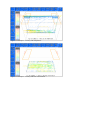
Figure 1: Vortex Setup Utility - File Manager
Figure 2: Vortex Setup Utility - Problem Configuration
Figure 3: Vortex Setup Utility - Global Settings
Figure 4: Vortex Setup Utility - Object Editor
Figure 5: Vortex Setup Utility - Mesh Generation
Figure 6: Vortex Setup Utility - Runtime Monitoring
Figure 7: Example 1 - Velocity and Temperature
Figure 8: Example 1 - Velocity and Temperature
Figure 9: Example 2 - Velocity and temperature
Figure 10: Example 2 - Velocity and Temperature
Figure 11: Example 2 - Velocity and TMRT
Figure 12: - Velocity and PPD
Figure 13: Example 3 - Velocity and Temperature
Figure 14: Example 3 - Velocity and CO2 concentration
9. INTRODUCTION TO FLOWVIS
There are often problems with existing visualisation systems. These include :·General purpose visualisation tools do not always treat fluid flow simulation data
correctly. There are instances where data is misplaced or misrepresented.
·Post processing visualisation of fluid flow data is one of the most important aspects of
simulation because the information and patterns in huge numerical data sets cannot be
interpreted without accurate visualisation tools.
·Many visualisation systems have over-complicated user interfaces with so much inappropriate functionality that users can be confused.
·Others provide cryptic command line interfaces that have intolerably high learning
overheads. This is often accompanied by endless questions for the settings associated with
a particular command.
·Where menu driven interfaces are provided these are often built onto command driven
code. This gives a user interface that can be complex to control because the underlying
development was command driven.
Why is FLOWVIS a better visualisation tool?
·FLOWVIS was designed primarily as a post processing tool for visualisation of fluid
dynamics data. The requirements were for intuitive user interaction and accurate
representation of simulation data.
·FLOWVIS development is driven by criticism of existing visualisation packages. This has
resulted in a system specifically for fluid dynamics researchers.
·The use of interactive interface techniques and intelligent default settings mean that
FLOWVIS is both easy to use and has low learning overheads for users. Productivity for
data analysis is enhanced by the interactive visual interface and the WYSIWYG view and
data selection menu.
·The development has initially been targeted specifically at PC platforms because of the
increasing use of PCs for fluid dynamics simulation. The package is highly optimised to use the
facilities of PCs for producing visualisations quickly and efficiently.
10. HARDWARE AND SOFTWARE REQUIREMENTS
FLOWVIS will run on IBM-PCs and most 100% compatible computers with the following
hardware and software minimum specifications :· 80486-SX processor (or higher specification processor).
· A colour VGA card for displaying a 640x480 pixels in 16 colours.
· Colour VGA monitor capable of displaying 640x480 pixels in 16 colours.
· 32 Mbytes or more of main system RAM.
· 10 Mbytes of available Hard-Disk space.
· Windows 95 and above (including Windows 98 or Windows NT)
· 3 button mouse and driver software (pre-installed before running FLOWVIS).
11. OVERVIEW OF FLOWVIS
FLOWVIS is a post processing visualisation system for use with structured mesh fluid dynamics
data. The system is fully menu driven using mouse or cursor selection. The main menu consists
of 20 icons that occupy the left and top edge borders of the screen. Generally the selection of an
icon will either initiate some action or invoke a sub-menu, which will pop-up over the central
portion of the screen.
Sub-menus generally have a common top row of buttons as [HELP], [EXIT], [RESET] and
([[DONE] or [DRAW]) from left to right. The rest of the menu will contain buttons, informative
text, displayed data and status fields and some menus have graphical display regions that will
contain images. Most of the menus are treated as forms that have a number of default values.
The user can change these values by pressing (selecting-on) the associated buttons. When a menu
contains the correct information the [DONE] (or [DRAW] on display-command menus) button
will initiate the action required for that menu.
FLOWVIS only allows the selection of buttons. The data fields cannot be altered by selection on
the data field itself. This strategy was adopted to avoid the confusion found with some other user
interfaces where users are not sure which menu items they can and cannot select. Often the
selection of an option will be followed by an automatic shift of the cursor to the next most logical
option. For example the FILE MANAGER menu will shift the cursor from a button that selects a
file to the [OPEN] file button ready for that action. Another example of the automation in
FLOWVIS is the fact that the VIEW SELECTION menu is always presented after the FILE
MANAGER menu has been used. This is useful as the next operation, after loading a new dataset, is usually to select the data region to be viewed and the view orientation.
FLOWVIS uses a data-base of files for visualisation. There will generally be more files in the
data-base than there were input files. This is necessary because most CFD output files are
designed to store data compactly but are not very fast to access. The FLOWVIS data-base is
optimised for fast access and contains many calculated values which are not present in the original
input files. The data-base creation routine can be accessed from within the FLOWVIS file
manager and there is a command line version. The data-base files for FLOWVIS are easily
identified by the three character extension which starts with an “F”. For example the file with
extension “.FHD” is the header information for this data-set. One data-set uses the same eight
character name for all associated files.
When [OPEN] is selected, for a data-base, in the FILE MANAGER all the data-base files are
connected for reading. At this stage FLOWVIS is ready for your visualisation commands.
The main menu consists of icons on the left and top edge of the screen. The left edge has display
commands e.g. VECTORS, CONTOURS and GRID etc. The top border has options for system
configuration, file management, orienting the view and textual notation etc. The options have
internal checks to prevent meaningless actions so that time wastage is kept to a minimum. An
example of this is that menus are inactive until a data-set is connected. Also the PRINT option is
disabled until there are some saved commands to redraw.
One of the main features of FLOWVIS is the command stack that saves commands for subsequent
replay. As a drawing command is completed the command and associated settings are saved to
the stack. The stack also maintains the view orientation in up to four windows. Automatic
checking prevents commands that would produce meaningless displays. Examples of these
checks include:1.Only one data-set can be used in one window.
2.There can only be one active view per window.
3.Graphs cannot be mixed with other commands in one window except text.
If a possible conflict occurs FLOWVIS will prompt you for keeping the existing display or
updating the display. It must be stressed that updating the display can mean that previous
commands are purged depending on the type of conflict.
The fact that FLOWVIS maintains a view for each display window means that up to four
differently oriented views can be shown on screen simultaneously. The view menu can be used in
conjunction with the redraw option to change the orientation of display elements in one window.
If the currently set view is different from the view in a target window, as a command is about to
be drawn, FLOWVIS will ask if the view should be updated or the command displayed using the
previous view. If the display is updated to the new view orientation then the previous commands
will be replayed to create the composite display in the new orientation.
There are a number of ways of saving images from FLOWVIS. Standard hard-copy to file is
provided in HP-GL, PostScript and Raster formats. These files have to be created by redrawing
all the commands in the display. An alternative is the PCX screen dump facility which captures
the entire screen and saves it as a PCX file. Finally there is a facility for bitmap image saving and
loading which can be used for screen-shot slide shows. These bitmap images are not printable
and are not particularly compact but have the advantage of fast display.
The displays created by FLOWVIS are mostly created on a plane by plane basis. The exceptions
are streamlines and contour nets which are continuous through the volume of the domain.
FLOWVIS warns you about view orientations that present the planes edge on rather than flat on
the screen. FLOWVIS will also attempt to draw certain commands in such a way that minimal
overwrite occurs.
This is achieved by trying to create the display drawing from deepest to nearest screen depth
coordinate. This technique is by no means infallible but generally produces acceptable displays.
Finally the drawing commands can be broken into and stopped. There are two different ways of
stopping drawing. The first is to use the [ESC] key or the right hand mouse button. This will
cancel the current operation and will not save the command to the redraw stack. The second
break
in
action
uses
the
numeric
keypad
[ENTER] key or the middle mouse button. Although this terminates the current drawing
operation it will still save the command to the redraw stack for subsequent redrawing.
12. GETTING STARTED WITH FLOWVIS
If you want to use a mouse with FLOWVIS then your mouse software driver should be loaded into
memory before you attempt to run FLOWVIS. The FLOWVIS executables MUST be invoked
with the batch script files that are present in the directory called FLOWVIS. These scripts are
tailored to your particular installation and set some environment variables for use by FLOWVIS.
If you do not have any prepared FLOWVIS data-sets then you must create some before you can
visualise any data. The FLOWVIS data-sets can be created from the command line using the
FILTER utility or using the [CREATE] option from within the FLOWVIS FILE MANAGER
menu. See the section in this manual on “CREATING A FLOWVIS DATA-SET”.
The FLOWVIS script file optionally takes a data-base case name argument. This feature allows
FLOWVIS to immediately load the named data-set. If no case is specified or the case was not
found then an introduction screen will be displayed. At this point you can use a mouse or
keyboard selection to confirm any options. Mouse selection is simply a matter of highlighting the
button you wish to operate and then selecting with the left mouse button. The cursor keys can
also be used for changing the highlighted button and the [SPACE] or [ENTER] keys will operate
the button.
If no file has been pre-loaded (see above) then the first menu automatically presented is the FILE
MANAGER menu. This allows you to change directory (if required) and to open a named dataset for visualisation. If you wish to change drive you must use the button marked [PATH]. This
feature is a little awkward on DOS systems but has the advantage of maintaining compatibility
with unix workstations where there are no named drives to access. The main facility provided by
the FILE MANAGER is to [OPEN] a new FLOWVIS data-set for visualisation.
Once a file has been loaded the FILE MANAGER menu automatically dismisses and the
DISPLAY MENU will appear. This menu provides options for changing the number of windows
used in the display. You can experiment with any of the features here but the default
configuration can be used simply by pressing the [DONE] button.
The VIEW SELECTION menu is also automatically presented. You should use the view selector
to choose the extent of the data you want to be used for subsequent drawing commands. The
VIEW SELECTION menu should also be used to set the orientation used to draw any of the
display commands. The menu has a graphical area that provides comprehensive and interactive
visual feedback of the set view orientation and the extent of the data selected. When you have set
the required view and data-extent you can select [DONE] to return to the main menu. At this
point FLOWVIS is ready and waiting for your display commands.
At the main menu the icons at the left side and top of the screen can be selected by mouse or
cursor keys and [ENTER] to confirm. Most of the icons pop-up a menu over the centre of the
screen. The options for displays to be created are on the left of the screen. Although many of the
display menus look quite complicated the use of intelligent defaults means that very few options
actually need to be changed. Generally only the variable used or type of display will have to be
changed for visualisation
13. MAIN MENU OPTIONS
The main menu options are described in general overview of the functionality. If the main menu
option opens a sub-menu then the reference material for each of the buttons in the sub-menu is
described.
Sub-menu descriptions are generally supported by a graphical image that shows the screen
representation of the open menu. Where collections of buttons are associated with a single data
field their functionality is described as a group.
There are essentially three types of button in sub-menus. The first type change the value of a
parameter that is displayed in a data display field. This may involve the addition or subtraction of
a value or stepping through a set of options. These buttons are often labelled as [<], [>], [-] or [+].
Occasionally it is necessary for a button to change the parameters displayed in a number of the
display fields.
Another type of button opens a textual input line where characters or numbers can be entered.
These buttons often have the label [SET] to indicate the manual setting of a value.
Finally there are “do-it” buttons that immediately initiate some action. The [DRAW] and [EXIT]
options are examples of buttons which immediately perform some action.
Most of the sub-menus are form menus. The parameters can be modified until all of the
selections are as desired then a single button selection initiates the functionality of the menu using
the selections in the form. Almost all of the sub-menu parameters are defaulted to sensible values
so there are generally only minimal changes required to draw a picture element.
EXIT
Exit overview
Exit allows you to quit from FLOWVIS and return to the operating system. The user is prompted
for confirmation of selecting quit.
If the exit is confirmed FLOWVIS will check the redraw stack for drawing commands. If there
are commands in the stack then you will be asked if you want save the stack as a file.
Just before FLOWVIS terminates any temporary files will be deleted and all open files will be
closed. Finally the normal text screen is restored.
GRAPH
Graph overview
The graph option allows up to ten graphs to be specified for one target window. These graphs can
be for any cell line within the data-set. The choice of cell line (and the range of cells) is achieved
by selecting the data plane that contains the line of cells, the range of cells in the cell line and the
other line index which identifies one particular line of cells from the plane. The limits of cells
along the chosen line are termed the “BASE RANGE”, The coordinates of the cells in the
specified range are plotting along the horizontal (or base) axis of the graph. Any one of the
variables from the data-base may be used as the vertical axis.
Most of the GRAPH MENU contains options associated with one particular graph-line selection.
The [BACK] and [NEXT] options can be used to access any one of 10 line-graph settings.
Options are provided for markers, drawing a smooth spline of the data points, changing colours,
changing line type and for scaling or shifting a particular graph. There is also access to a visual
data selection menu which indicates a line of cells. This can be used to interactively choose the
graphing location with visual feedback confirmation. The menu used for data selection is very
similar to the VIEW SELECTION menu except that the view orientation, in this menu, is only for
your convenience and is not used with any other displays.
When you select [DRAW] to display the specified graphs FLOWVIS automatically scales all the
graphs to fit within the target window. The graphs are saved to the redraw stack and when graph
is selected again (for a particular window) all of the specifications will be available for
modification.
FLOWVIS allows you to access other data-sets simultaneously for graphing. The [FILE] button
actually brings up the FILE MANAGER menu in the correct mode for opening a data-base. The
active data-base name, for each graph, is displayed next to the [FILE] button.
Graph options
Use the [HELP] button to enter help mode for the GRAPH sub-menu. The selection of any button
in help mode will bring up help for that button or group of buttons. The help mode is exited by
selecting on the [HELP] button again. The [F1] key will also perform the same action but will
present help for the last highlighted button.
The [EXIT] option allows the GRAPH sub-menu to be exited without any changes taking effect.
This action can also be performed with the [ESC] key or the right-hand mouse button. No
attempts are made to do displays and changes to parameters will be lost.
The [DEFAULTS] option resets the default parameters in the GRAPH menu. This provides a
quick way of returning to sensible values.
The [DRAW] option takes all of the GRAPH specifications and calls the graph display routine. In
displays
with
more
than
one
window
FLOWVIS will draw the graphs in the same window as was chosen when the main menu GRAPH
option was selected. All of the specified graphs are re-drawn from scratch. If there is any conflict
of the graph commands with existing display commands then you will be asked if you require the
existing commands to be kept or discarded and replaced by the graphs.
The [BACK] and [NEXT] Graph menu options are provided to step through the individual graph
specifications. The actual graph specification being modified is indicated by the numbers
displayed above these buttons. Each graph uses the whole menu as a form that specifies only that
one graph. The other graph specifications are then accessed by stepping forwards and backwards
through the forms. This will often be accompanied by a number of changes in the data display
fields.
The Graph [FILE..] option allows other data-sets to be accessed for graphing. These are opened
in the file manager menu. The filename displayed to the right of the file button indicates the dataset from which this particular graph will be drawn. The selection of variable and the cell extent
will be set appropriately for this data-set.
The clear [THIS] and [ALL] options are used to clear one or all of the graph specifications
respectively. This is accomplished by setting the variable for one or all graphs to “NULL”. The
graphs with “NULL” as the variable are ignored when draw is selected.
The [GLOBAL...] option will be available soon to provide facilities for global graph settings.
These facilities will include access to the graph title and labelling of axes, graph graticules, axes
settings and presentation styles. This is to be implemented as another menu which will exit back
to the graph specification menu.
The [DATA...] option opens a visual menu provided for interactive selection of the line of cells to
be used for graphing. The data selection menu is very similar to the main view menu but is
restricted to selecting only one line of cells. The menu does feature the view orientation options
of the main view menu but any changes made in this menu are not used in subsequent displays.
The data selection menu exists back to this graph specification menu and updates the cell line
extent for the current graph element.
The variable selection [<<] and [>>] options allow the variable used for the current graph element
to be selected. These buttons scroll through the entire list of variables that are available in the
current data-base. The selected variable is indicated by name above the buttons. A “NULL” in
the variable name field means that the current graph element is inactive as no variable has been
chosen.
The [SLAB], [<] and [>] options allow the graphing data plane to be selected. This is one stage
of the selection of a line of cells. The plane or slab orientations is chosen with the [SLAB] button
as an X, Y or Z plane and the [<] and [>] buttons step through the available planes by index. The
actual plane currently selected is indicated by the display fields above these buttons. The chosen
plane is the plane that the line of cells will be taken from for graph display for this particular
graph element. The Base range and Line options are used to select the exact line of cells used for
this graph element. Changing the plane orientation automatically changes the base range and line
orientations because they must all be mutually exclusive directions. Data-sets which are 2Dimensional will not permit the plane orientation to be altered.
The [BASE] orientation and base limits [<][>], [<][>] options are provided to choose the
orientation and extent of the line of cells used for this graph element. The direction of the line of
cells and the end limits are displayed above these buttons. Once a plane orientation has been
selected there are only two possibilities for the base-range direction. The exact cell line to be
used is not specified fully until the third coordinate direction index is selected.
The cell line [<] and [>] options allow the third coordinate index for this graph element to be
selected. The direction and index are indicated above the buttons in the display fields. The
direction cannot be changed because the plane and base directions have already been selected
leaving the third coordinate direction for this option.
The variable scale [SET], [<] and [>] options allow the scale of the variable to be changed for this
graph element. By default the scale value is 1.0 which does not scale the values of the variable.
The scale value can be set explicitly using the [SET] option or stepped to using the [<] and [>]
buttons. The scale is applied by multiplying the value in each graph cell by the scale value.
Negative numbers are allowed.
The variable shift [SET], [<] and [>] options allow the variable axis to be shifted. By default this
shift value is set to 0.0 implying no shift. Positive values have the effect of increasing all of the
values of this variable whilst negative values decrease all the variable values. The [SET] button
allows explicit selection of a shift value whereas the [<] and [>] buttons step incrementally.
The base scale [SET], [<] and [>] options are used to scale the coordinate axis of the current
graph element. The scaling is applied by multiplying every coordinate point in the graph by the
scale value. By default this value is set to 1.0 implying no scaling. The [SET] option can be used
to set the coordinate base scale explicitly whilst the [<] and [>] buttons step incrementally to a
value.
The base shift [SET], [<] and [>] options allow all of the points in this graph element to be
coordinate shifted by the shift value set here.
A positive value increases the coordinate values whilst a negative value decreases the coordinate
values. The [SET] button allows the shift value to be typed in explicitly whilst the [<] and [>]
buttons step incrementally to a value. The line type [-] and [+] options allow the line style for this
graph element to be changed from the default. There are options for dotted, dashed, dot-dashed
and no-lines. The graph element is drawn using the indicated line type. When “NO-LINES” is
selected the markers will be used to show the graph location.
The colour [-] and [+] options allow the colour of each graph element to be selected. The colours
scroll through a list of named colours. The colour used for this graph element is the one named
above the buttons in the display field. The marker type [-][+] and marker character [-][+] options
allow the selection of a particular type of marker to be used for this graph element. The marker
types are marker, letter and number or none and there are ten choices for the character used. The
markers indicate the locations of the actual data point (x,y) pairs on the graph element. Also the
specific key label has the appropriate marker type for referencing the correct graph element.
The spline [ALTER] option allows a graph element to be drawn with a smooth spline. When
spline is used there may be overshoots where there is a very sudden change in gradient but for the
most part spline produces a smooth curve through the data points.
The [KEY] label facility allows you to input a limited amount of text to reference individual
graph elements. Currently 10 characters are allowed. These form a reference key drawn to the
side of the graph. Markers (if used) identify the specific keys to graph elements but also the keys
are coloured similarly to the appropriate graph.
The [LogV] and [LogB] options allow the graph variable and / or base axis to be logged. This
will only be appropriate if all of the values are positive otherwise the request is ignored. It should
be stressed that mixing log and non-log graphs together may have the effect of minimising one of
the graphs almost to obscurity because of the automatic scaling and the ranges of values.
STREAMLINES
Streamline overview
The formal definition of streamlines states that streamlines are, at all points, tangential to the local
velocity field. FLOWVIS allows a 2-Dimensional plate region to be seeded with streamlines
which can then be followed forwards or backwards.
The streamlines are, by default, coloured by the local velocity magnitude but can also be coloured
by any data-base variable or in a single colour.
The number of streams seeded can be selected from 1 to 250. These are scattered regularly on the
seed region. The accuracy of the streamlines can be selected using the streamline steps parameter.
This indicates how many steps of calculation should be used to get across a cell. The larger this
value the more accurate the streamlines (and the longer the display takes). The plate region for
streamline seeding can be selected from indicated indices or from a plate (or slab) data selection
menu. The SLAB SELECTION menu is very similar to the VIEW SELECTION menu but the
orientation within the slab menu is not used in any other displays.
Streamlines, particularly ones which get caught in recirculations, may not terminate so
FLOWVIS imposes a number of termination conditions. After a set number of stream following
steps the user is prompted for continuing to following the streamlines.
FLOWVIS will not follow a particular streamline if it exits the domain or if it appears to stop.
The second condition is necessary because streamlines are independent of time and the scaling of
very small local velocities could produce spurious results.
When the streamlines are drawn some may appear to advance faster than others. There is NO
physical significance in this and it is merely a feature of the streamline tracking algorithm used.
Streamline options
Use the [HELP] button to enter help mode for the STREAMLINES sub-menu. The selection of
any button in help mode will bring up help for that button or group of buttons. The help mode is
exited by selecting on the [HELP] button again. The [F1] key will also perform the same action
but will present help for the last highlighted button.
The [EXIT] option allows the STREAMLINES sub-menu to be exited without any changes taking
effect. This action can also be performed with the [ESC] key or the right-hand mouse button. No
attempts are made to do displays and changes to parameters will be lost.
The [DEFAULTS] option resets the default parameters in the STREAMLINES menu. This
provides a quick method of returning to sensible values after experimentation.
The [DRAW] option takes all of the STREAMLINE settings and calls the display routine. In
displays with more than one window FLOWVIS will prompt for the target window in which to
display STREAMLINES. Streamline following will proceed until all of the streams have been
terminated or a number of cells have been stepped through. If there are still streams active when
the preset number of steps have been reached then FLOWVIS will prompt for streamlines to
continue for a similar number of steps.
The [<][>], [Min] and [Max] options allow the number of seeding points for Streamlines to be
selected. The specified number of seeds are then placed regularly in the selected seed region.
The seed region is a given 2-Dimensional plate within the domain.
The colours [<] and [>] options allow the number of colours used for following Streamlines to be
set. The default is the maximum number of colours available. This option only has effect
between the specified range of colours. It is used for limiting the number of colours used from a
potentially large range of colours.
The Colour Range upper limit [<][>] and lower limit [<][>] options allow the actual colour range
used to be selected. The colours range from red as the lowest number to blue which is the highest.
The range can be reduced, reversed or switched to white only by using the middle mouse key.
The seeding region [MENU...] option brings up a visual menu, similar to the main menu view
option, for selecting a streamline seeding 2-Dimensional plate. This plate can also be selected
using options in this menu. The plate (or slab) forms the region over which the streamline seeds
are placed.
The Streamline plane [NEW], [<] and [>] options allow the seeding slab to be changed to an X-,
Y- or a Z-plate and the number of the slab to be chosen. The streams will be seeded regularly over
the extent of this slab. For 2-Dimensional domains these options have no effect.
The seeding slab ranges [<][>][<][>] options can be used to reduce the extent of the seeding
region down from the whole plane to a sub-region. The extent is specified by cell indices and the
data-base directions are displayed above the ranges.
The Streamline [FOLLOW] option allows the direction in which the streamlines are followed to
be specified. When the streamlines are followed forwards the velocities are used as they are in
the data-base. Following backwards uses the negated velocity components found in the data-base.
The streamline [USING] option allows streams to be tracked in the whole domain or optionally
only in the current view selected region. If a seed starts outside of the region (or leaves the
region) it will not be followed any further.
The Stream steps [<] and [>] options allow the streamline refinement to be specified. This integer
value determines how accurately (and fast) the Streamlines are followed. The larger the value the
more steps are used to follow the Streams. More accuracy does mean that the stream following
will be slower.
The kill at edges option has not yet been implemented.
The stream colouring [USE] options allow the type of stream coloration to be selected. The
choices are for local resultant speed, single colour or using a data-base variable for coloration.
The colouring used is indicated just below the [DRAW] button.
The scroll [TOP], [LAST], [UP] and [DOWN] options allow other portions of the variable list to
be displayed. This is necessary where the full variable list is larger than the visible portion of the
list. The [USE] buttons allow the adjacent variable names to be selected.
GEOMETRY
Geometry overview
Geometry is supported in two distinct ways. The first is by porosity specified geometry given as
field (or cell) values in the data set. This can be cell porosity (Volume PORosity) or face
specified porosities for high-x (East PORosity), high-y (North PORosity) or high-z (High
PORosity). These geometrical features are displayed as filled cells or tiles respectively. The fill
and edge colours can be selected for these volume or face porosities. By default the volume
porosity geometry routine uses an algorithm which sorts the cells into furthest to nearest order and
displays them using hidden line techniques. Whilst this takes a little while to sort the cells in
order it does produce pleasing displays because the “block” objects have a solid appearance.
The other form of geometry supported is by user defined features. These are entered as
commands which display boxes, arcs, lines, poly-lines and polygons etc. These commands (and
their associated parameters) can also be interpreted from a geometry file.
Two other commands (OPEN and CLOSE) allow interactively specified geometry to be saved to a
file. This is necessary if the geometry is to be saved to the redraw stack. Closing the geometry
file causes the commands to be available for redrawing. The geometry menu also has an option to
bring up the file manager for choosing an existing geometry file for replay.
FLOWVIS does not check the type of file that is requested for geometry so the user must be sure
that the file does contain geometry commands.
Geometry commands
The commands and parameters used for specifying user defined geometry are:OPEN <filename>
Which opens a named new file for saving geometry commands or opens a file for replay.
CLOSE <filename>
Which closes the named or currently open file and ensures that it will be available for redrawing.
ARC line colour circ
+ x1 y1 z1
+ x2 y2 z2
+ x3 y3 z3
Draws an arc using three coordinate points on the arc. If circ is 1 then a circle will be draw rather
than just an arc for a value of O.
the command is typed over four lines using the + to indicate successive lines of input.
BOX x1 y1 z1 x2 y2 z2
Draws a box with diagonally opposite corner coordinates at (x1,y1,z1) and (x2,y2,z2).
LINE x1 y1 z1 x2 y2 z2
Draws a line from the coordinate point (x1,y1,z1) to point (x2,y2,z2).
PLINE x1 y1 z1 (line) (colour)
+ x2 y2 z2
+ ...
+ xn yn zn
Draws a poly line for the given coordinate specified points. The continuation character + is used
to add points over subsequent lines of input. At least 2 points must be given in which case a
single line is displayed.
PGON x1 y1 z1 (line) (fill)
+ x2 y2 z2
+...
+ xn yn zn
Draws a polygon for the given coordinate points. The continuation character + is used to add the
next line segment. The polygon will only be displayed after the last line of input. End of input is
indicated when a blank line is entered.
GRID OUT orient plane OR
GRID OUT orient plane dir1 lim1 lim2 dir2 lim3 lim4
Draws the grid outline for the given plane or the specified region. The ORIENTation,
DIRection_1 and DIRection_2 are one of “X”, “Y” or “Z” and must be exclusive so that each
appears only once. The PLANE-number and LIMits are cell index numbers for the indicated
directions. For example:GRID OUT X 3 Y 1 15 Z 2 4
will display the grid outline of plane X = 3 for the Y and Z limits given.
EXIT (or \)
Quits from interactive geometry specification.
HELP (or ?)
Brings up on-line help.
HELP <Command_name>
Brings up help about a specific command.
Comments can start with # or REM and are ignored by the interpreter.
N.B. Parameters in parenthesis (option) are optional and names in angle brackets <name> should
be replaced by the required name for that action.
Use the [HELP] button to enter help mode for the GEOMETRY sub-menu. The selection of any
button in help mode will bring up help for that button or group of buttons. The help mode is
exited by selecting on the [HELP] button again. The [F1] key will also perform the same action
but will present help for the last highlighted button.
The [EXIT] option allows the GEOMETRY sub-menu to be exited without any changes taking
effect. This action can also be performed with the [ESC] key or the right-hand mouse button. No
attempts are made to do displays and changes to parameters will be lost.
The [DEFAULTS] option resets the default parameters in the GEOMETRY menu. This provides
a quick method of returning to sensible values after experimentation.
The [DRAW] option takes the GEOMETRY settings and calls the display routine. In displays
with more than one window FLOWVIS will prompt for the target window in which to display
GEOMETRY. The interactive GEOMETRY option displays the user-defined geometry and exits
back to the main menu automatically.
The volume porosity [VPOR] option allows volume porosity to be used (if available) for
displaying blocked cells. If no volume porosities are present in the data-set then this option will
not be available. The style of displaying cells is set using the options below [VPOR].
The face porosity [EPOR], [NPOR] and [HPOR] options allow blocked faces (defined by
porosities) to be displayed. If there are no face porosities defined in the current data-set then
these options cannot be activated. The style of display for the blocked faces can be selected using
the options below the face porosity buttons.
The [LOAD FILE..] option allows the user to load and display the geometry commands from an
ascii geometry file. This option brings up the FILE MANAGER menu to return a file name. The
user must be sure that the selected geometry file does indeed contain geometry commands
because FLOWVIS does not check the type of file. The results could be unpredictable if a binary
file were opened and interpreted.
The edge colour [<] and [>] options for volume porosity cells allow the cell bounding edges to be
displayed in a different colour to the faces. This option is used for the cell edges regardless of the
status or colour of the faces.
The edge colour [<] and [>] options for face porosities allow the face bounding edge colour to be
specified. The edges will be displayed in this colour regardless of the settings of face fill colour
or face fill status.
The interactive [GEOMETRY..] option allows the user to enter geometry commands into an
interpreter for the display of user-defined objects in the data-domain. The commands include
coordinate specified boxes, arcs, polygons, poly-lines and cell region specified grid outlines.
There are also open and close file commands that allow the typed commands to be saved to file
for subsequent replay by the redraw facility.
The interactive geometry [MENU..] option is not currently available. This is being developed to
provide interactive user defined geometry specification. These facilities will be available with
future upgrades to the FLOWVIS system.
The fill colour [<] and [>] options for volume porosity blocked cells allows the colour of the cell
faces to be selected. This option will be ignored if the volume porosity fill option is set to NOfill.
The fill colour [<] and [>] options for face porosities allow the colour of the faces to be selected.
This option will be ignored if the face porosity fill option is set to NO-fill.
The hidden line [HIDE] option is currently under development to allow the display of user
defined geometry objects using hidden line techniques. This option will be ignored by this
version of FLOWVIS but will be supported in future upgrades.
The volume porosity [FILL] option allows the faces of blocked cells to have solid filled faces in
the colour specified by the fill colour option.
The volume porosity [HIDE] option allows cells to be displayed using hidden line techniques.
These are slower but do prevent overwriting by cell faces that are deeper into the domain.
The volume porosity [TYPE] option specifies the speed with which the cells should be displayed.
The fast option merely displays the cells in a far to near order so that near cells are not obscured.
The slow option sorts the cells accurately by screen depth but does produce a more pleasing
display.
The face porosity [FILLED] option allows blocked faces to be drawn using solid colour fills. The
colour used will be the one specified in the face porosity fill colour option. The fill and colour
options for faces have effect for all three cell face directions.
The user defined geometry [FILL] option is not currently available. When supported it will allow
user defined objects to have filled faces where appropriate. This feature will be provided as an
upgrade.
GRID
Grid overview
The grid display routine has options for cell centred, face centred or grid outlines. These are
displayed at the mid-plane position. This is consistent with most of the other display routines
which display properties at the cell centres. The two types of grids and grid outlines are only
displayed for the currently selected data region.
VECTORS
Vectors overview
Vectors are plotted for orthogonal sets of vector components. The vector arrows are displayed at
the centre of the cells within the domain. The values used are interpolated to the cell centres from
the faces of cells. The vectors are automatically scaled to the average cell size. This helps to
prevent vectors from overwriting portions of other adjacent vectors. There is a manual scaling
utility to adjust the size of the vectors in situations where automatic scaling is unsatisfactory.
Vectors can be coloured by magnitude, any single variable from the data-base or single-coloured.
The colouring ordering can be chosen to run from RED=greatest_value to BLUE=smallest_value
or as RED=smallest_value to BLUE=greatest_value. The values concerned are the minimum and
maximum values associated with the current domain or data region. See the SETTINGS MENU
for information about the minimum and maximum scan options.
The vector sets are determined as the data-base is created and the selection of which vectors to
display is then a simple matter of choosing the required set. The actual names of the components
(in a set) are displayed at the bottom of the menu. The default set is always the cartesian
component set for the first phase. Cylindrical polar data sets have their vector components
resolved to cartesian componets at the data-base creation stage.
The vector menu contains a number of options to change the appearance of the vector arrows.
The actual vector appearance is indicated by the graphical display area. This graphics box
contains a representation of a vector arrow and a cell (a box drawn with a dotted line).
One other feature of the vector menu is the magnitude range selection. This indicates the current
range of magnitudes in the data set for the currently selected region. The actual range displayed
can be changed. This has the effect of discarding vectors which are outside of the specified
range.
Vectors options
Use the [HELP] button to enter help mode for the VECTOR sub-menu. The selection of any
button in help mode will bring up help for that button or group of buttons. The help mode is
exited by selecting on the [HELP] button again. The [F1] key will also perform the same action
but will present help for the last highlighted button.
The [EXIT] option allows the VECTOR sub-menu to be exited without any changes taking effect.
This action can also be performed with the [ESC] key or the right-hand mouse button. No
attempts are made to do displays and changes to parameters will be lost.
The [DEFAULTS] option resets the default parameters in the VECTOR menu. This provides a
quick method of returning to sensible values after experimentation.
The [DRAW] option takes the VECTOR settings and calls the vector display routine. In displays
with more than one window FLOWVIS will prompt for the target window in which to display
VECTORS. The vectors will be displayed for the currently selected data region using the active
view orientation.
The vector head open [>] and display [>] options allow vectors to be drawn with closed heads or
without arrow heads respectively. The appearance of the vectors is shown in the box to the lefthand side of the menu.
The colours in range [<][>] and [Min][Max] options allow the use of a limited number of colours
rather than the whole range of available colours. The default is to use the full range of colours.
The colour range high limit [<][>] and low limit [<][>] options allow the range of colours used to
be changed. The default is for the maximum allowed range of colours with red as the lowest
valued and blue as the highest. The range can be reduced, reversed or swapped to white only
(using the middle mouse button for selection).
The show vector [SYMBS] option allows the display of symbols to represent vectors which are
nearly directly towards or away from the screen and therefore cannot be displayed as arrows. The
symbols used are a cross for a vector tail (vector into the screen) and a circle for a head (vector
coming out of the screen). The symbols are shown in the appearance graphics box if activated.
The vector set [-1] and [+1] options allow the selection of other orthogonal vector sets for display
(if these are available in the current data-set). The component names for the indicated set are
shown at the bottom of the menu for the X-, Y- and Z-components. By default the first set is
always the first phase cartesian component set (if any vector sets are defined).
The colour [BACK] and [NEXT] options allow the type of vector colouring to be selected. The
default is to use the resultant magnitude (size) for colouring but any variable from the data-base
can be used.
The colour range and number of colours are used as defined in those options.
The magnitude range upper limit [<][>] and lower limit [<][>] options allow the vectors to be
displayed for a limited range of magnitudes. The full range of vector magnitudes is the default
and these values are displayed between the upper and lower limits.
The show vector [DOTS] option allows tiny vector components (that cannot be displayed as
arrows) to be drawn as dots. These dots tend to clutter up the display if activated so this option
has been provided to remove them.
The vector scale [LARGE] and [SMALL] options allow the displayed arrows to be scaled up or
down in size. A value of 1.0 is the normal size based on averaged cell dimensions.
The vector head size [INCR] and [DECR] options allow the size of the vector arrow heads can be
made larger or smaller depending on the value set for this option. The range is 0.1 to 0.9 times
the overall vector arrow length.
The vector head angle [+] and [-] options allow the splay angle of the vectors to be set. The value
is between angles of 5 and 80 degrees. The appearance of the vector arrows is visible in the
vector appearance box on the left of the menu.
The X-, Y- and Z- component [+] and [-] options are not currently available. The display fields
do show the current components for the indicated set. These options are being developed to allow
any scalar variables to be treated as orthogonal vector components. These facilities will be
available as an upgrade in the near future.
CONTOUR LINES
Contour lines overview
Contour lines use a single data-base variable to draw coloured iso-valued lines on a plane by
plane basis for the current view region.
There are options for altering the colour range, the range of contour values and the number of lines that are displayed.
A single contour line is displayed using the “CONTOUR VALUE” option or a number of lines
can be displayed equally spread over a “CONTOUR RANGE” of values.
By default the contours are displayed using one line for each of the available colours and the full
range of values of the chosen variable.
The list of variables on the right hand side of the menu scrolls to allow access to any of the
variables in the data-base. The current contouring variable is displayed just below the [DRAW]
button.
The contour line display is the default but there are also options for a contour peak plot or a
contour surface (net) plot. The contour peak plot uses the value of the variable being contoured
to raise or lower the contour line from the plotting data-plane. This produces a 3-Dimensional
surface when viewed from near edge on..
The “HEIGHT SCALE” option is used in conjunction with contour peak plots to manually adjust
the height of the 3-Dimensional contour surface above the data-plane.
The contour net facility follows contours through three directions in 3-Dimensional space to form
surfaces of equal contour value. The surfaces have the appearance of a net and hence the name
contour nets. These contour nets cannot be displayed for 2-Dimensional data sets.
The resolution parameter termed “Resolved Pixels” determines how finely the contouring units
are sub-divided so that the contour lines can be plotted. A small value will produce a more
accurate display but will also take longer to draw.
Contour lines options
Use the [HELP] button to enter help mode for the CONTOUR-line sub-menu. The selection of
any button in help mode will bring up help for that button or group of buttons. The help mode is
exited by selecting on the [HELP] button again. The [F1] key will also perform the same action
but will present help for the last highlighted button.
The [EXIT] option allows the CONTOUR-line sub-menu to be exited without any changes taking
effect. This action can also be performed with the [ESC] key or the right-hand mouse button. No
attempts are made to do displays and changes to parameters will be lost.
The [DEFAULTS] option resets the default parameters in the CONTOUR-line menu. This
provides a quick method of returning to sensible values after experimentation.
The [DRAW] option takes the settings and calls the appropriate contouring display routine. In
displays with more than one window
FLOWVIS will prompt for the target window in which to display contour-lines. The contours will
be displayed for the currently selected data region using the active view orientation.
The contour colour range upper limit [<][>] and lower limit [<][>] options allow the colour range
used for contouring to be selected.
The integer numbers displayed represent colours given that the lowest number represents red and
the highest is blue. The range can be reduced, reversed or swapped to white only.
The [DO] contour LINE option is the default option for this menu. When this option is selected
the contour plot will be of normal contour lines. The [DRAW] option must be used to start
drawing the contours. The variable used for contouring is that indicated by the current contour
variable text in the top right corner of the contour line menu.
The [DO] contour PEAK plots are available from this menu. These are formed by projecting the
contours away from the data-plane by an amount which is proportionate to the value of the
contour line value. These plots only have significance if viewed nearly edge on. The height scale
option allows the height of the peaks to be changed.
The [DO] contour NET displays allows contour surface plots to be created. These can only be
displayed for 3-Dimensional data-sets.
The surfaces are displayed throughout the domain. Again the contour variable is that indicated in
the top right corner of the menu.
The contour variable [USE] options allow a named variable to be selected from a scrolling list.
These options make the adjacent variables current and the current variable is used for the contour
plot when [DRAW] is selected.
The scroll buttons [UP], [DOWN], [TOP] and [LAST] can be used to access more variables than
can be displayed on the visible portion of the list. All of the variables from the data-base are
presented in the list for contouring.
The number of contour lines [-] and [+] options are used to select the actual number of lines used
for the contour plots. This can be larger than the number of colours available but this will
produce plots that have a number of contours of the same colour.
The colours in range [LESS], [MORE], [MIN] and [MAX] options are used to select the number
of colours to be used from the colour range. The default is the same as the number of colours in
the colour range. This option is really only provided for using less than the maximum number of
colours but still taken from the full range of colours.
The contour value [<] and [>] options allow a single contour value to be selected for display by
the contour routine. The default and alternative to this option is to use a range of values.
The resolved pixels [-] and [+] options allow the refinement of the contour display to be specified.
A low value means that cells are sub-divided for more accurate contours. Accuracy does imply a
slower display. The numbers actually represent the number of screen pixels that are used as a test
for suitable refinement.
The height scale [DECR] and [INCR] options set the scale value for contour peaks. This
parameter is used to adjust the height of the peaks from the plane. The scaling is automatic based
on averaged dimensions but this option provides an override.
The minimum [<<][>|] and maximum [|<][>>] options allow the range of contour values to be
limited. By default this is set to the full range for the currently selected variable but a sub-range
of values can be selected. If a sub-range is chosen then contours outside of this range are not
displayed.
CONTOUR FILLS
Contour fills overview
Contour fills draw solid filled contours for a chosen variable. Filled contours are also drawn on a
plane by plane basis. The filled contours are actually ranges of contour values (bands) which are
all coloured similarly within each range. The ranges are determined by sub-dividing the full
range of values of the selected variable by the number of contours to be used in the display.
The choice of colours used is specified by the colour range and colours in range options. The
colour range determines which colour represents high values and which represents low values
given that colour number 1 is red and colour number 13 (at least on 16 colour displays) is blue.
Three colours are reserved for the background, foreground and grey colours. The “COLOURS IN
RANGE” option allows a sub-set of colours to be used from the full range.
Other than the default option for contour fills the FILL MENU also has options for fill peak maps,
solid filled cells and block filled cells. The fill peak maps are analogous to the contour line peak
plots and display a 3-Dimensional surface by raising the pixels being filled away from the dataplane by an amount which is proportional to the value of the variable at that point. The height
scale option can be used to alter the height of the 3-Dimensional peaks from the data plane.
Contour fills overview
The contour filled peak plot should only really be used for a single data plane and for best results
this plane should be viewed from near edge on. The filled cells option takes the field value within
a cell and fills the whole cell according to that value. This can be useful for data analysis
because the value displayed will be the same as that used in the numerical simulation code that
produced the results. The block filled cells again uses the field value of a variable in a cell but
draws a 3-Dimensional brick in an appropriate colour. The height of the block is proportional to
the value of the variable. This option gives the appearance of a 3-Dimensional histogram for a
plane of data.
Use the [HELP] button to enter help mode for the contour-FILL sub-menu. The selection of any
button in help mode will bring up help for that button or group of buttons. The help mode is
exited by selecting on the [HELP] button again. The [F1] key will also perform the same action
but will present help for the last highlighted button.
The [EXIT] option allows the contour-FILL sub-menu to be exited without any changes taking
effect. This action can also be performed with the [ESC] key or the right-hand mouse button. No
attempts are made to do displays and changes to parameters will be lost.
The [DEFAULTS] option resets the default parameters in the contour-FILL menu. This provides
a quick method of returning to sensible values after experimentation.
The [DRAW] option takes the settings and calls the appropriate contour fill display routine. In
displays with more than one window FLOWVIS will prompt for the target window in which to
display fills. The fills will be displayed for the currently selected data region using the active
view orientation.
The colour range upper limit [<][>] and lower limit [<][>] allow the range of colours used in the
fill displays to be selected. The range can be reduced or reversed for contour fills. The low
valued colour is red and the high value is blue.
The [DO] CONTOUR FILL option is the default for this menu. The contour fill uses the current
variable and settings to produce solid filled contour bands for the current data region. The
contour fill display is initiated by selecting on the [DRAW] button.
The [DO] FILL PEAK MAP option allows a 3-Dimensional raised surface plot to be created. The
height of the surface above the plane is proportionate to the local value being contour filled hence
producing a terrain type plot with mountains and valleys. These only have significance if viewed
nearly edge on. The height scale allows the height of the peaks to be changed.
The [DO] FILLED CELLS option produces a plot with solid filled cells where each cell has one
colour appropriate to the selected variable field value within that cell.
The [DO] BLOCK FILLS option uses a single data plane to draw hidden line blocks of
appropriately scaled height and colour. These are most effective when viewed from near edge on
to the plane as they produce a 3-Dimensional histogram of the data values on a data plane. The
height scale options can be used to scale the height of the blocks.
The fill variable [USE] options allow a named variable to be selected from a scrolling list. These
options make the adjacent variables current and the current variable is used for the fill plot when
[DRAW] is selected.
The scroll buttons [UP], [DOWN], [TOP] and [LAST] can be used to access more variables than
can be displayed on the visible portion of the list. All of the variables from the data-base are
presented in the list for contour filling.
The colours in range [LESS], [MORE], [MIN] and [MAX] options are used to select the number
of colours to be used from the colour range. The default is the same as the number of colours in
the colour range. This option is really only provided for using less than the maximum number of
colours but still taken from the full range of colours.
The fill value [<] and [>] options allow a single contour fill value to be selected for display by the
contour filling routines. The default and alternative to this option is to use a range of values.
The resolved pixels [-] and [+] options allow the refinement of the contour fill display to be
specified. A low value means that cells are sub-divided for more accurate filled contours.
Accuracy does imply a slower display. This actually represents the number of screen pixels that
are used as a test for suitable refinement.
The height scale [DECR] and [INCR] options set the scale value for contour fill peaks and block
fill plots. This parameter is used to adjust the height of the peaks from the plane. The scaling is
automatic based on averaged dimensions but this option provides an override.
The minimum [<<][>|] and maximum [|<][>>] options allow the range of contour fill values to be
limited. By default this is set to the full range for the currently selected variable but a sub-range
of values can be selected. If a sub-range is chosen then contour fills outside of this range are
displayed as for the extreme limits of the fill colour bands.
HELP
Help overview
FLOWVIS has an on-line help system that is accessible from the main menu and pop-up submenus. Help mode is entered by selecting on the [HELP] option or by pressing the [F1] key. The
help system will then display a message in the top half of the screen to inform you that the system
is now in help mode and an information box towards the bottom of the screen that contains the
help text. (The format for displaying sub-menu help is identical). Once help mode has been
entered the system waits for you to select on an option. Selecting any valid option will bring up
the on-line help associated with that button. Finally the help mode is exited by again selecting on
the [HELP] option or pressing [F1].
The main menu help system gives general help about the main menu options whereas the submenu help gives specific help about options or groups of options within individual menus.
FILE MANAGER
File manager overview
The FILE MANAGER menu has facilities for opening various types of file, moving through the
hard-disk directory structure, making directories, erasing individual files and data-sets and for
creating FLOWVIS data sets from input files containing field data.
Usually the FILE MANAGER is used to load a data set. The files used by FLOWVIS are all
named by an 8 character case name. This identifies all of the files of the particular case.
FLOWVIS uses the 3 character extension to determine the purpose of individual case files. You
should not rename FLOWVIS case files individually but you can rename all of a case. e.g. you
may rename a data-set called “OLDCASE” to “NEWCASE” using the DOS command:RENAME OLDCASE.f* NEWCASE.f*
FLOWVIS will then be able to connect “NEWCASE” for analysis and visualisation.
FLOWVIS only has one data set attached at a time but keeps the case names in the redraw stack
for seamless visualisation of more than one data-set. You should not erase data sets for which
there are commands in the redraw stack as FLOWVIS will not be able to redraw these commands.
When [OPEN] is selected, for a data-base case, any previously open data-base files are closed and
the new ones opened. The [SEARCH] option is provided so that FLOWVIS is aware of the type
of file you are trying to open. The search pattern specifications are:“*.DAT”
This is for input data files that need to be converted to the FLOWVIS format. This is only for
preference. FLOWVIS will actually create a data-case from any named file provided it is a field
data file.
“*.FHD”
This stands for FLOWVIS HeaDer files. These contain the general information about the datacases that inform FLOWVIS about the number and type of field variables stored and the extent
and size of the data domain.
“*.DSC”
These files contain saved stack information. Loading a stack file in the file manager will cause
the commands in that stack to be replayed. The data-sets used in a stack must still exist in the
same directory location for FLOWVIS to be able to replay the commands.
“*.*”
This search pattern displays all of the files in the current directory and can be used for browsing.
There is currently a limitation of 250 file name entries in the current listing.
The current directory path is displayed at the top of the menu next to the [PATH] option.
FLOWVIS requires that you use the [PATH] option to change drives on DOS systems. This is
necessary for maintaining compatibility with unix-like systems where there is no such concept as
a drive. You may also use [PATH] to type in a known path without having to use multiple [CD]
selections to navigate the directory structure. If a full typed path is incorrect then FLOWVIS
leaves the path that was previously set. This is also true of disk drives that do not exist or empty
floppy drives.
If you get lost in a directory structure then the [HOME] option can be used to return you to the
directory that FLOWVIS was initially run from.
The FILE MANAGER is also called by several other menus for getting an existing file name or for
just opening a new data-set if required. When the FILE MANAGER is used in this mode it will
not allow you to change the search specification and the menu itself will only pass back the filename and path requested by the calling menu when [OPEN] or [DONE] are selected.
See the manual section about “CREATING A FLOWVIS DATA-CASE” for details of preparing
field data files for visualisation by FLOWVIS.
Opening a file is achieved by selecting on the [>] button next to the required file. This name will
then become visible in the FILE = <filename> display field and the cursor moves to highlight the
[OPEN] button. Selecting on the [OPEN] button will then open that file and close the FILE
MANAGER menu.
File manager options
Use the [HELP] button to enter help mode for the FILE MANAGER sub-menu. The selection of
any button in help mode will bring up help for that button or group of buttons. The help mode is
exited by selecting on the [HELP] button again. The [F1] key will also perform the same action
but will present help for the last highlighted button.
The [EXIT] option allows the FILE MANAGER sub-menu to be exited without any changes
taking effect. This action can also be performed with the [ESC] key or the right-hand mouse
button.
The [HOME] option sets the current directory path to the start-up directory path regardless of the
current path or drive. This is useful if you get lost in an obscure directory.
The [FINISH] is use to exit from the FILE MANAGER. No data is lost and any attached files
remain so. A file must be [OPEN]ed for viewing before any of the other main menu display
commands become active.
The [PATH] option can be used to jump to a known directory path. This must be typed in full
using the text input box. The alternative is the scrolling list of directories on the right. The
[PATH] option must be used to change disk drives on DOS based systems. If the typed path does
not exist then the previous path will be restored.
The [CHDIR..] option allows the current directory to be set to the parent directory. This is a way
of navigating back up a directory structure. See also [Home] to get to the home directory.
The file and directory [UP], [DOWN], [TOP] and [BOTTOM] options are used to scroll the file
and directory name lists. The file and directory lists maintain file and directory names for the
current path. These lists can be scrolled (if required) by using the scroll buttons provided. The
selection buttons for the lists are provided on the left.
The file pattern [SEARCH] option allows the file search extension to be changed. A formatted
data-base is “*.FHD”, all files are “*.*”, stack files are “*.DSC” and unformatted input files are
“*.DAT”. When FLOWVIS is requested to search for FLOWVIS data-cases only the 8 character
identifying name is displayed in the file name list.
The file list [>] options allow the adjacent filename to be made current. The current file is shown
by the FILE=<filename> message.
This filename is used for the options in the bottom left of the FILE MANAGER menu.
The directory list [CD] options perform a change of directory to the named directory immediately
below the current path. The [Home] option can be used to return to the start-up directory if the
user becomes lost.
The [OPEN] file or case option uses the current file to try to load a file. If the FILE MANAGER
is being used for data-base access then all files for that case are opened and all other files closed.
If the search pattern is set for a previously saved stack file then the stack file is loaded and
replayed. The FILE MANAGER can also be used by other menus to return a file name and a
directory path. These are returned when the [OPEN] or [FINISH] buttons are selected.
The [MKDIR] option allows the creation of a named sub-directory below the current path or at a
fully specified path. The name must be typed in the text input box.
[ERASE] allows a single file to be deleted or an entire case with all associated files. The Shell
tool will provide an alternative means of executing OS commands when available.
The [SHELL] operating system shell option is currently under development. When available it
will provide facilities for file copying, deletion and renaming, etc. This will be provided as an
upgrade.
The [FILTER] facility is currently under development. When available it will provide access to
data-base manipulation routines. These capabilities will be provided as an add on enhancement to
FLOWVIS.
The [CREATE] a FLOWVIS data-case option manipulates an input data file to produce a
FLOWVIS data-set. The data-base can be created from this option or from the command line
utility provided with FLOWVIS. After creating a data-set FLOWVIS will ask if you now want to
load the data-set for visualisation and analysis.
VIEW SELECTION
View selection overview
The VIEW SELECTION menu provides facilities to set limits for the data region to be used for
subsequent displays and to set the view orientation that any data is displayed from.
The view menu consists of three vertical sections. The left most section allows the data extent to
be limited and the plane type to be selected. The selection of a data region is indicated by the cell
indices in the three orthogonal data-base directions X, Y and Z. The extent of the data to be
visualised by subsequent commands is then indicated by three pairs of low and high cell index
limits. A visual feedback of the selected region is visible in the graphical area as the solid-line
boundary.
The cell limits can also be selected by coordinate values. These are the [SET] buttons near the
cell limit indicators. Using set will present a text input bar which will display the current
coordinate range for the chosen direction. Once you have entered the required range the
coordinates will be mapped to the nearest cell indices.
The middle section of the view menu contains a graphical representation of the data domain and
the selected data region. Also present are the data-base coordinate axes, the view rotation axes
(labelled H, V and D) and if the data-set contains volume porosity data there will also be points
indicated to show the location of blocked cells.
The domain outline is shown dotted and the selected region is shown as a solid-line boundary.
Generally speaking the image in the graphics area will change interactively as the view menu
options and parameters are changed. Also this image represents the images that will be produced
in the display area windows. This is not strictly true of target display windows which have a very
different aspect ratio from the view menu graphics area. In these cases the height of the image in
the target window is approximately proportionate to the height of the image in the view menu.
This means that short, wide target windows will show an image which is well in from the left and
right borders if they were touching in the view menu and that tall, thin target windows will
generally loose the left and right edges of the image. It is recommended that the display type be
selected so that the windows match the shape of the domain as closely as possible.
Finally the right most side of the view menu has the options for view orientation manipulation.
These include zoom-in, zoom-out, rotation (about three orthogonal directions) using the indicated
--> H,
--> V and --> D axes and finally image positioning by stepped shifting in a vertical
or horizontal direction. Again these options have immediate visual confirmation from the
graphical area.
These options should be used to orient the data on screen as you require it to be drawn by
subsequent display commands. If you loose sight of the domain or get an obscure view then the
[RESET] option can be used to reset the default view. Selecting [Done] will then return to the
main menu ready for drawing (or redrawing) commands using the newest view settings.
The view menu is also seen in three slightly different forms for getting region, slab and line limits
respectively. In these data selection menus the view orientation options still work within the menu
but are not used to update the current orientation settings. These menus are used to visually
select regions for use by the GRAPH and STREAMLINE options.
View selection options
Use the [HELP] button to enter help mode for the VIEW SELECTION sub-menu. The selection
of any button in help mode will bring up help for that button or group of buttons. The help mode
is exited by selecting on the [HELP] button again. The [F1] key will also perform the same action
but will present help for the last highlighted button.
The [EXIT] option allows the VIEW SELECTION sub-menu to be exited without any changes
taking effect. This action can also be performed with the [ESC] key or the right-hand mouse
button.
The [RESET] option will reset all of the view orientation settings to the default values. This can
be invaluable when the domain has been moved of the screen or zoomed in too far.
The [DONE] option implements all of the changes made in the menu and exits from the menu.
This contrasts with [EXIT] which discards any changes made. Control returns to the main menu
ready for visualisation commands. The view orientation settings are always compared with the
view selection of windows with existing commands. FLOWVIS will not permit two different
views to be mixed in a window so you will be prompted (as you try to draw or redraw) if the
views have changed. The choice presented is to use the existing view or to update the window to
use the new view.
The [PLANES] option allows the orientation of data to be selected. Since most of the display
commands are drawn plane by plane this will determine how the displays are created. The View
menu has three data selection forms that only allow selection of a region, slab or line of cells.
These are used by other menus that need to allow a region to be selected visually. The equivalent
buttons in the three data selection menus are [SLABS], [SLAB] and [LINE].
The zoom setting [SET ZOOM], [IN] and [OUT] options allow the level of zoom to be set
explicitly or incrementally. The display field shows the level of zoom as a real number. A zoom
value of 1.0 is normal size whilst -ve values zoom out and +ve zoom in. A factor of 2.0 for
example makes the object twice the size. The [SET ZOOM] option uses a text-input box to
prompt for a real value. The zoom will change the appearance of the view seen in the graphical
area of the menu. Use zoom to bring the domain closer or to zoom into a specific area.
The X-cells range lower limit [<][>|] and upper limit [|<][>] options are provided to allow the
selection of the range of cells from which data will be viewed in the X coordinate direction (in
Cylindrical Polar coordinates this is the angle direction). These options change the cell indices
incrementally.
The X-cells range [SET] option uses a text input box for the entry of two coordinate X values
which are converted to the nearest cell indices. When called the current coordinate range is
displayed. The full range of cells in this coordinate direction is indicated just above the button.
The move [SET], [<] and [>] options allow for shifting the display horizontally. The value
displayed is a percentage of the maximum data-base dimension. This value can be set explicitly
or interactively using the two buttons below the indicator. The effect of shift horizontally is to
move the image within the display area. A value of 0 means that the display is centred
horizontally.
The move [SET], [v] and [^] options allow for shifting the display vertically. The value displayed
is a percentage of the maximum data-base dimension. This value can be set explicitly or
interactively using the two buttons below the indicator. A value of 0 means that the display is
centred vertically.
The [ZERO] option centres the data-base in the centre of the screen. This is used for bringing the
image back into view when it has been shifted too far from the centre. The effect is analogous to
setting both the horizontal and vertical shift values to zero.
The move to [EDGE] option is currently under development. This will shift and zoom the database for the maximum possible screen usage. This feature will be available as an update.
The [SET ROTATION] option allows all three axial rotation angles to be set explicitly in a text
input box. The ordering is H-axis, V-axis then D-axis rotation in that order. The rotations will be
applied in that order. Since rotations are non-commutative it is critical that the order be observed.
This option is provided to repeat known rotations as displayed by the rotation angles given below
this option. The alternative is to use the interactive mode which is more intuitive because the
rotations are applied to the graphical image area incrementally.
The Y-cells range [SET], lower limit [<][>|] and upper limit [|<][>] options are provided to allow
the selection of the range of cells from which data will be viewed in the Y coordinate direction (in
Cylindrical Polar coordinates this is the radial direction). The [SET] option uses a text input box
for the entry of two coordinate Y values which are converted to the nearest cell indices. When
called the current coordinate range is displayed. The other options change the cell indices
incrementally. The full range of cells in this coordinate direction is indicated just above the
buttons.
The rotation [H-], [H+], [V-], [V+], [D-] and [D+] options allow incremental rotation about the
screen-(H)orizontal, screen-(V)ertical and screen-(D)epth axes respectively. The rotations are
applied about either global or local orthogonal axes. The global axes remain fixed in space
whereas the local axes follow the domain as it is rotated. The angles for each axial rotation
represent the angles that would need to be applied in a (H, V, D) order to get to the same resultant
image. This is necessary for the [SET ROTATION] option which allows all three axial rotations
to be set explicitly. The angle step size is set in the SETTINGS MENU but is by default 5
degrees. Because of the nature of rotation the numerical angles displayed do not necessarily
change predictably BUT the object does rotate predictably which is somewhat more important.
The Z-cells range [SET], lower limit [<][>|] and upper limit [|<][>] options are provided to allow
the selection of the range of cells from which data will be viewed in the Z coordinate direction (in
Cylindrical Polar coordinates this is the length direction). The [SET] option uses a text input box
for the entry of two Z coordinate values which are converted to the nearest cell indices. When
called the current coordinate range is displayed. The other options change the cell indices
incrementally. The full range of cells in this coordinate direction is indicated just above the
buttons.
DISPLAY SELECTION
Display selection overview
The DISPLAY MENU provides various facilities for configuring the display. The three main
features are the type of coordinate mapping, the colour key settings and the number and type of
windows used in the main display area.
The coordinate mapping can be either parallel projection or perspective projection. By default the
perspective projection is used for 3-Dimensional domains (because it gives a more realistic
appearance) and parallel is used for 2-Dimensional domains.
The key legends for colour displays are boxes that indicate the values associated with colours for
certain commands. For example a vector display can have a key that indicates that vectors
coloured in red have a certain magnitude whilst vectors coloured in blue have a different
magnitude. There are options for how the key is to be placed and the type of key to be drawn.
The placement can be “automatic” in which case FLOWVIS places the keys or “manual” in
which case the key is placed as an outline by using the mouse.
There is a third option which makes FLOWVIS ask how the key should be placed every time.
Currently there is only a choice of drawing a vertical key or not having any keys at all. The
display area can have up to four separate windows. The options for the type of windows are
available at the bottom of the DISPLAY MENU. The choices of windows range from one window
which uses the whole of the display area to four quarter-windows. The current selection is
indicated by a pictorial representation of the main display area, in the graphics box at the bottom
of the menu.
Display selection options
Use the [HELP] button to enter help mode for the DISPLAY sub-menu. The selection of any
button in help mode will bring up help for that button or group of buttons. The help mode is
exited by selecting on the [HELP] button again. The [F1] key will also perform the same action
but will present help for the last highlighted button.
The [EXIT] option allows the DISPLAY sub-menu to be exited without any changes taking
effect. This action can also be performed with the [ESC] key or the right-hand mouse button.
The [RESET] option resets the parameters in the DISPLAY menu back to the default settings.
The [DONE] option performs an exit from the DISPLAY menu but any changes made are left
intact. Control passes back to the main menu. If the window configuration has changed then
FLOWVIS will re-display the main graphics area with the new windows. If there are commands
in the stack then FLOWVIS will ask if you wish to proceed with the re-configuration. Sometimes
keys (which have absolute screen pop-up locations) do not go well in other windows.
The fit to window [STRETCH] option allows the selected data region to be stretched out to fill the
whole screen. This does not preserve the aspect ratio of the domain but can be useful for
visualising long, thin domains.
The type of coordinate mapping is specified by the [PROJECT] option. FLOWVIS supports both
parallel and perspective projections. Perspective gives 3-Dimensional domains a more realistic
look on the screen but 2-Dimensional domains use parallel projection by default.
The delete before draw [DEL] option allows FLOWVIS to clear the screen before every drawing
command is executed. By default FLOWVIS places images one on top of another, where
possible. This option allows each display to be drawn on a clear screen. All commands are still
be saved in the stack for redrawing.
The key location [LOCATE] option informs FLOWVIS how to place the colour keys for coloured
vector, streamline and contour displays.
Options are AUTO-matic, ASK as required and MANUAL which allows interactive key
placement. The manual mode means that the key bounding box is displayed under user control
and can be positioned interactively on the display. FLOWVIS uses pop-up keys that are removed
when a new command is targeted on a window and replaced after the command has been drawn.
The key format [KEY] option only allows keys to be drawn vertically or not drawn at all. The
keys contain numerical and colour mapping information for contour, vector and streamline plots.
It is intended that horizontal keys will be provided in future versions of FLOWVIS.
The delete all windows [ALL DEL] option configures how the main menu {DEL] option works.
When this option is set a single selection if delete will clear all windows and remove the last
redraw command from each window (for multi-window displays). This option has no effect for a
single window display.
The [WHOLE], [VERTICAL], [HORIZON], [RIGHT 2], [TOP 2] and [QUARTER] options
determine how the main display area is divided into windows. Each of the configured windows
can have individual view orientations. These options provide a variety of window groupings as
shown in the graphics box. When multiple windows are used for display FLOWVIS will ask you
to select in a window to indicate where commands are to be displayed.
TEXT
Text overview
The text option allows displays to be annotated with text and, optionally, to have a pointer arrow.
The text to be displayed is typed into an input box and when [ENTER] is selected a rectangular box appears in the
target display window.
This box is the outline of the text to be displayed. Selecting a location and pressing the left mouse
button will result in the placement of the text at that position. Then FLOWVIS will ask if you
require a text pointer. If you require a pointer this is placed interactively by selecting a point for
the tail and then selecting a point for the head. Depending on the configuration of FLOWVIS an
arrowhead can optionally be drawn on the pointer.
There will shortly be available a menu for the selection of font and text colour. This will be
available as an upgrade.
REDRAW
Redraw overview
The redraw command takes all the commands for a window and replays them after first clearing
the window. The redraw ordering can be by the drawing order or by a logical order that was set to
prevent certain commands from obscuring other commands. The choice of the ordering is set
within the SETTINGS MENU.
Redraw can also be used to redraw more than one window if the Redraw Globally option has been
set in the settings menu.
When a stack file has been loaded the redraw option can be used to replay the commands saved
there.
By default the main menu [DEL]ete option clears the window and removes the last command
from the redraw stack for that window. If there were many commands in a window then doing a
redraw will re-display all the commands left for that window.
One further feature of REDRAW is that if the view orientation has changed from that of the
commands already in a window and redraw is requested then FLOWVIS will ask if the commands
should be redrawn using the previous or the newest orientation. See also the notes on the VIEW
MENU operation.
STACK
Stack overview
The redraw stack is the repository for all successful drawing commands. The stack can be
thought of as a number of slots into which commands and all their associated parameters and
attributes can be saved. There are also a number of slots, which store window specific
information so that views do not become muddled (at least that is the intention!). The stack
actually resides in a file like structure that can be physically saved to a permanent file for
subsequent reuse by FLOWVIS. Since this file only contains the commands (but no data) the data
sets that originally created the displays must still exist for successful replay of the stack.
Furthermore the data sets must exist in the same locations because FLOWVIS keeps track of
absolute paths to the data sets.
The stack file cannot be edited by hand as the commands and parameters are stored in binary
access format.
Work is progressing on an editing facility which will allow commands to be pulled back into their
menus for modification. This facility will be available with upgrades of FLOWVIS.
DELETE
Delete overview
The main menu [DEL]ete command has several different configurations but in its most basic form
it clears a target window and removes the last added command (for that window) from the redraw
stack.
When the display is set to one window then delete will bring up the previous picture automatically
(as if the last command had not be selected).
Delete can be used to clear all windows and optionally to remove all commands from the redraw
stack. See the DISPLAY MENU and the SETTINGS MENU information for more details.
In displays with more than one window delete will prompt you for a target window in which to
delete.
A message will be posted onto the screen when the redraw stack for any window has been
emptied.
PRINT
Print overview
FLOWVIS can produce hard-copy output files in a number of formats but does not print directly
to printers. This is necessary because of the vast range of printers, printer drivers and languages
for graphics printers.
FLOWVIS can produce two distinct types of image. The first is bitmapped images that are
essentially screen dumps in various formats. These have a set resolution that is dependent on the
screen resolution from which they were produced. The second type are vector graphic image
formats that store a list of object definitions to re-create the final image. These are not limited to
the screen resolution and generally produce much better hard-copy results on suitable printers.
Vector graphic formats generally do require performance printers and can be very large files.
Currently the printer file-creation drivers in FLOWVIS have to redraw the whole display whilst at
the same time creating the required hard-copy file. Since most users will not require the main
menu to be printed the print option will redraw on the full screen as it creates the hard-copy
output. FLOWVIS will then wait for user input from the mouse or keyboard. This allows video or
photographic images to be captured if required.
The [OK] prompt box that appears at the bottom right hand corner of the display means that
FLOWVIS is waiting for interaction after having created any required hard-copy output. The
middle mouse button can be used to hide the [OK] box if necessary.
The image formats supported are HP-GL, PostScript and Raster. There is also a PCX screen
grabbing utility built into FLOWVIS that can be activated by pressing [ALT] and [F2] together.
This is almost always available except when text input is occurring to a text box.
The PCX grab utility will capture the whole screen including any menus or message text that may
be present. A single speaker tone means that PCX file creation has started and two tones indicates
that the PCX file has been created.
Generally all hard-copy files are saved in the current directory and have filenames made up of
three parts. The first part is an identifier of 4 characters that you may specify for recognising the
plot files. The second part is an incremented number (starting at 0001) that FLOWVIS adds to
make sure that any existing plots are not overwritten. Finally the extension indicates the type of
hard-copy file. The extension “.HPG” is for HP-GL files, the “.PS” extension indicates
postscript files, the extension “.RAS” indicates Raster files and “.PCX” extensions are for PCX
bitmapped images.
Print options
Use the [HELP] button to enter help mode for the PRINT sub-menu. The selection of any button
in help mode will bring up help for that button or group of buttons. The help mode is exited by
selecting on the [HELP] button again. The [F1] key will also perform the same action but will
present help for the last highlighted button.
The [EXIT] option allows the PRINT sub-menu to be exited without any changes taking effect.
This action can also be performed with the [ESC] key or the right-hand mouse button. No hardcopy output or full-screen display will be created if this menu is exited.
The [DEFAULTS] options will be available to reset the default print settings.
The [PROCEED] option performs the required hard-copy print and display. This will generally
involve redrawing all picture elements on the full screen. This is necessary for hard-copy file
creation because of the nature of the print drivers. When the full screen has been created
FLOWVIS draws a small box marked [OK] in the bottom right of the screen and waits for some
interaction via the mouse or keyboard. This facility is provided to allow video or photographic
Image capture from screen. The [OK] box can be removed by pressing the middle mouse button.
The printer driver [USE] options allow specific hard-copy printer files to be created. The
currently supported selection includes HP-GL, PostScript and Raster image output. These files
will be created in the current working directory.
The hard-copy status [HARDCOPY] option informs FLOWVIS to create hard-copy output as files
defined by the formats above. If output is disabled then a full screen image is created but no hardcopy files are produced.
SETTINGS MENU
Settings menu overview
The settings menu allows many of the default settings in FLOWVIS to be changed. Some of the
most useful are:Domain and Region Outlines:
This turns on or off the automatic display of the boundaries of the whole domain and currently
selected data region respectively.
Min and Max Scanning:
This indicates to FLOWVIS how the colour range is to be scanned for the values in a given data
region. The domain option means that minimum and maximum values will be those of the whole
domain rather than just the selected data region. The plane option uses only those planes which
pass through the data region for minimum and maximum scanning whilst the region option
actually checks only those cells within the specified data-region to find the minimum and
maximum. These options are necessary when you want to use the full range of colours (for a
small region) even when the region may have only a small range of values within it.
Redraw ordering:
As mentioned in the redraw option the stack commands can be drawn in a logical order to prevent
(as far as possible) overwriting. The alternative is to draw the commands in the first drawn order.
Plane Steps:
This parameter tells FLOWVIS to skip planes (where possible) when creating displays. This has
the effect of rarefying the data when there is too much to visualise comfortably and when the
screen becomes cluttered. Values of zero means do not skip any p1anes. Streamlines and graphs
ignore this parameter completely. Contour lines, fills and grids skip planes only and vectors skip
cells in all three data-set directions.
There are also a number of parameters for controlling the default step sizes used in the VIEW
SELECTION menu.
Settings menu options
Use the [HELP] button to enter help mode for the SETTINGS sub-menu. The selection of any
button in help mode will bring up help for that button or group of buttons. The help mode is
exited by selecting on the [HELP] button again. The [F1] key will also perform the same action
but will present help for the last highlighted button.
The [DONE] option performs an exit from the SETTINGS menu and returns to the main menu to
await further commands.
The show outlines [DOMAIN] and [REGION] options allow displays to be configured to draw
the outlines of the whole domain and the currently selected data-region respectively. These
appear as dotted grey and solid white bounding lines respectively.
The choose window [CHOOSE] option informs FLOWVIS to prompt for a target window in
multiple windowed displays. This option can be made to keep the current window active without
prompts for a choice of window. By default FLOWVIS always prompts for a target window when
there are more than one windows.
The min and max scan [SCAN AS] option allows colour coded pictures to use different minimum
and maximum values for scaling. The options are for whole DOMAIN, whole PLANES that cut
the data region or as the current active REGION. By default the DOMAIN is used for scanning
minimum and maximum values because colour scaling for sub regions will be consistent
anywhere in the domain. The REGION option is used where features cannot be seen because of a
large range of values in the whole domain but small ranges within a selected data region.
The rotation type [ROTATE] option allows the rotation axes to be LOCAL or GLOBAL.
LOCAL axis rotation moves the rotation axes with the domain whereas global axes are fixed in
space and the domain moves past. Changing this option while there are existing stack commands
may have undesirable results in terms of the images produced.
The redraw ordering [AS] option allows the saved stack commands to be replayed in a LOGICAL
or the actual DRAWING order. The logical order helps to prevent display corruption and image
overwrite by re-ordering the commands.
The redraw globally [GLOBAL] option allows the main menu [REDRAW] command to operate
on all windows of a multiple windowed display. The alternative is for redrawing in a chosen (or
active) window only. In the case of multiple window displays FLOWVIS will prompt for the
target window for redrawing.
The default zoom [<] and [>] options allow the default zoom value to be set. This will be the
value set for the zoom factor whenever [RESET] is selected in the VIEW menu in the current
session.
The redraw after printing [+REDRAW] option allows the graphics image to be restored along
with the main menu after a full-screen print. Alternatively FLOWVIS will merely replace the
main menu after clearing the screen. The commands in the redraw stack are unaffected.
The delete removes all commands [REMOVE] option allows delete to remove all of the
previously saved commands from the redraw stack when delete is selected. Use this option with
caution because deleted commands are NOT retrievable. The default usage only allows the last
command to be removed.
The zoom step sizes [LESS] and [MORE] options allow the size of zoom steps in the VIEW
menu can be set. A smaller value gives greater control but also takes longer to make large
changes in the zoom factor. Note that the VIEW menu does provide accelerated stepping for
incremental options by using the middle mouse button.
The plane steps [-] and [+] options inform FLOWVIS to skip over cells where possible. In most
cases this will result in stepping over planes only but vector displays step over cells in all three
index directions whilst streamlines cannot step over cells at all.
This facility can be useful for huge data sets where images can become cluttered by the amount of
information displayed.
The show views similarly [SAME XYZ] option allows the view onto the data-base to be
independent of the type of plane selected in the VIEW men. This contrasts with bringing the
selected plane flat onto the screen by applying default rotations.
The angle step size [LOW] and [HIGH] options allow the view menu rotation steps size to be
changed. By default the angle step size is 5 degrees but this may be increased or reduced here.
The step size is the number of degrees added to (or subtracted from) the current rotation about one
axis.
SYSTEM
System overview
This option is provided to allow future enhancement of the settings available with FLOWVIS.
This functionality will mirror the control provided by FLOWVIS initialisation files. These
facilities will be available as with upgrades.
EXPERT
Expert overview
The EXPERT MENU is similar to the main menu SYSTEM option in that it allows for future
enhancement of FLOWVIS. The functionality to be added here is of a more practical nature than
the system settings options. The reason for including the menu now is that the remainder of the
FLOWVIS user interface will not have to change significantly (even as planned extensions are
added). The enhancements to change significantly (even as planned extensions are added). The
enhancements already being developed are listed in the section “PLANNED EXTENSIONS TO
FLOWVIS”.
Currently there are three facilities provided in the menu:1
The demonstrator shows some saved images that were captured in internal image format and
saved to disk files.
2
The menu re-display option redraws the whole screen in full.
3
The slide utility allows internal screen images to be saved to or loaded from files. These
images require an eight-character identifier to which FLOWVIS adds an extension, which
indicates the screen mode that the images come from. You cannot load images into different
screen modes, than they were produced from, as this can lead to unsatisfactory or corrupted
displays.
The screen image demonstrations were produced by the screen image LOAD and SAVE utilities.
You can replace the existing “SCREEN??.SM1” files with your own if you require demonstration
facilities of your own data sets.
LIMITATIONS OF FLOWVIS (Version 3.10)
1 Only databases of size 70 cells by 70 cells by 70 cells by 50 variables are currently supported.
There is also currently a restriction of 70 cells in any one direction. These limitations are
being removed in future releases of FLOWVIS. Please contact the distributors if you have
special requirements.
2
The redraw stack can hold up to 100 commands. After 100 commands the redraw stack can
be saved and the existing commands overwritten. The stack always fills up from the start so it
is unlikely that this size limitation should be too critical.
3
Only 10 graphs can be displayed in any one window.
4
Changes to default values and settings within FLOWVIS cannot be saved for subsequent reuse. Future releases of FLOWVIS will allow modifications to be saved and loaded as
required. This is currently a way of tailoring the system by modifying the initialisation files
by hand.
5
Graphs and text can be mixed within a window. If the graph elements are modified after text
has been added then the text will be lost. There is also a limitation that text can only be added
to a window containing graphs since adding a graph to a window that only contains text will
result in the deletion of the text.
6
The colour key legends used in colour vectors, contour lines, fills and streamlines can be
placed manually. There is a potential problem if one key is placed on an existing key because
the pop-up key area saved can become corrupted. It is the responsibility of the user to make
sure that manually placed keys do not overlap.
KNOWN BUGS IN FLOWVIS (Version 3.10)
1 Streamlines do not yet use porosity values correctly. This can lead to situations where
streamlines enter blocked regions by up to half a cell. Work is in progress to correctly stop
the streamlines from entering blocked regions or passing through obstructions.
2
Streamlines suffer from accumulated integration errors. This is more noticeable for true
recirculations where there is a tendency for the streams to spiral outwards rather than meeting
the original stream after a circuit of the recirculation. One possible way to overcome this is to
have a fine grid.
FLOWVIS FACILITIES (Version 3.10)
User Interface
Menu driven with pop-up sub-menus.
Mouse pointing and selection.
Cursor-key navigation with space bar or return-key selection.
Intelligent next option selection in certain menus to speed up interaction. This involves
placing the cursor on the next sensible button ready for immediate selection.
Meaningful pop-up messages and critical action confirmation requests.
Automatic command saves for subsequent replay and possible save to file.
Break-in allowed on display creation by [ESC] or mouse button number [2] or [3].
Display
Up to four display areas (windows).
Up to four data sets on one display with one allowed for each window.
Pointing selection / cursor selection of active window for direction of output.
Selective redraw for all or single windows.
Choice of six-window configurations e.g. whole area, split horizontal or quarter etc.
Intelligent checking of display to prevent (as far as possible) corrupted displays caused by
inappropriate mixing of commands.
Textual annotation of displays.
Upgrade capabilities for 256 colour displays.
Upgrade facilities for very high resolution display modes (this requires a suitable graphics
card and monitor).
Visualisation Options
Contour line displays.
Contour fill displays.
Peak plots for 3-D visualisation of a data plane for contour fills and lines.
Filled cells for data analysis.
Filled cell 3-Dimensional histograms for a plane of data.
Contour line iso-surface nets through 3-Dimensional data-sets.
Vector displays for a vector set of up to three orthogonal components.
Grid displays for cell-faces, cell-centres or grid outlines.
Geometry display (defined by blocked grid cells with zero porosity).
User defined geometrical features formed from boxes, lines, arcs, etc.
Streamlines of Cartesian vector data.
Colour coded displays with associate colour keys that can be located manually.
Graph displays for lines of cells.
Data Selection
By region specified by orthogonal minimum and maximum cell index limits.
By entered physical coordinates that are mapped to nearest cell indices.
Has visual confirmation of data selection limits and shows the domain boundary.
Draws slab-by-slab for 3-D data region in a selected slab-wise direction.
Automatic warnings if selected planes are not flat onto screen.
View Selection
What-You-See-Is-What-You-Get view confirmation (this is consistent for windows of similar
aspect to the view-menu display area).
Three axes for combined rotations using global or local rotation strategies.
Zoom in or out.
Parallel (cabinet) or perspective 3-Dimensional projection.
Quick porosity geometry (if available) and local axes display for ease of orientation.
Move display within a window (up, right, down, left or centred).
Grid Types
2-D or 3-D structured meshes only.
Regular Cartesian, Cylindrical Polar or Body Fitted Coordinates.
User Preferences
Many features are set in run-time loaded files for easy configuration.
preferences will also be provided which can then be saved.
User defined
Hard-copy Output to File
Plot-file creation using redraw (uses incremental naming to prevent overwrites).
Support for Postscript, HP-GL and Raster formats.
PCX bit-mapped screen image saves.
Data-base Creation
Support for most structured mesh CFD code data formats. (Contact the Distributor for more
details).
Internal and external database creation tools to prepare data for visualisation by the FLOWVIS
system.
Data is displayed in the same form as it is used in the numerical simulation.
FLOWVIS presents data accurately for data analysis.
A fast access database is created for interactive visualisation but without extensive data
proliferation seen in many other visualisation systems.
Data sets are easily identifiable by case name and file extensions.
The filter source code can be made available for inclusion in third party CFD software for
seamless usage of FLOWVIS and your own CFD code.
Fast but comprehensive data preparations for quick image creation.
Potentially huge data sets can be visualised because FLOWVIS does not attempt to read all of
the data into memory at one time.
A Post Processing analysis tool specifically for Fluid Dynamics researchers
FLOWVIS is developed by CFD researchers for CFD users.
Interactive techniques give you a better feel for your data.
The production of high quality hard-copy files save you time.
The use of innovative display techniques presents your data in the most meaningful way
possible. The capabilities are also being continually enhanced.
PLANNED EXTENSIONS TO FLOWVIS
Display
Redraw editing past previous command deletion.
Presentation facility for screen displays.
User Preferences
Allow selective saving and loading of user defined defaults at runtime.
Access to low level colour palette.
Visualisation Options
Enhanced Graph facilities for annotation and presentation display style.
Particle tracking capability.
Display animation.
Operating System
Operating system interface for the target hardware.
Porting to workstation hardware platforms.
Utilities
Provision of data manipulation and preparation routines for input data files.
Research is being conducted into providing a limited capability CFD solver, with problem
specification routines, available within the FLOWVIS environment with suitable monitoring
capabilities. Whilst this cannot hope to be a competitor for commercial CFD solvers it will be
suitable for teaching purposes.