Download ST7 8-bit MCU family user guide

ST7
8-BIT MCU FAMILY
USER GUIDE
July 2002
1
USE IN LIFE SUPPORT DEVICES OR SYSTEMS MUST BE EXPRESSLY AUTHORIZED.
STMicroelectronics PRODUCTS ARE NOT AUTHORIZED FOR USE AS CRITICAL COMPONENTS IN
LIFE SUPPORT DEVICES OR SYSTEMS WITHOUT THE EXPRESS WRITTEN APPROVAL OF
STMicroelectronics. As used herein:
1. Life support devices or systems are those
which (a) are intended for surgical implant into
the body, or (b) support or sustain life, and
whose failure to perform, when properly used in
accordance with instructions for use provided
with the product, can be reasonably expected
to result in significant injury to the user.
1
2. A critical component is any component of a life
support device or system whose failure to
perform can reasonably be expected to cause
the failure of the life support device or system,
or to affect its safety or effectiveness.
Table of Contents
1 INTRODUCTION . . . . . . . . . . . . . . . . . . . . . . . . . . . . . . . . . . . . . . . . . . . . . . . . . . . . . . . . 12
1.1 WHO IS THIS BOOK WRITTEN FOR? . . . . . . . . . . . . . . . . . . . . . . . . . . . . . . . . . 12
1.2 ABOUT THE AUTHORS . . . . . . . . . . . . . . . . . . . . . . . . . . . . . . . . . . . . . . . . . . . . . 12
1.3 HOW IS THIS BOOK ORGANIZED? . . . . . . . . . . . . . . . . . . . . . . . . . . . . . . . . . . . 12
1.4 WHY A MICROCONTROLLER? . . . . . . . . . . . . . . . . . . . . . . . . . . . . . . . . . . . . . . . 13
1.4.1 Electronic circuitry . . . . . . . . . . . . . . . . . . . . . . . . . . . . . . . . . . . . . . . . . . . . . . . . . . . . . .15
1.4.2 Choice of microcontroller model . . . . . . . . . . . . . . . . . . . . . . . . . . . . . . . . . . . . . . . . . . .17
1.4.3 Choice of development tools . . . . . . . . . . . . . . . . . . . . . . . . . . . . . . . . . . . . . . . . . . . . .17
2 HOW DOES A TYPICAL MICROCONTROLLER WORK? . . . . . . . . . . . . . . . . . . . . . . . 19
2.1 THE CENTRAL PROCESSING UNIT . . . . . . . . . . . . . . . . . . . . . . . . . . . . . . . . . . . 20
2.2 HOW THE CPU AND ITS PERIPHERALS MAKE UP A SYSTEM . . . . . . . . . . . . 21
2.2.1 CPU . . . . . . . . . . . . . . . . . . . . . . . . . . . . . . . . . . . . . . . . . . . . . . . . . . . . . . . . . . . . . . . .21
2.2.2 Memory . . . . . . . . . . . . . . . . . . . . . . . . . . . . . . . . . . . . . . . . . . . . . . . . . . . . . . . . . . . . . .21
2.2.3 Input-Outputs . . . . . . . . . . . . . . . . . . . . . . . . . . . . . . . . . . . . . . . . . . . . . . . . . . . . . . . . .23
2.2.4 Interrupt Controller . . . . . . . . . . . . . . . . . . . . . . . . . . . . . . . . . . . . . . . . . . . . . . . . . . . . .24
2.2.5 Bus . . . . . . . . . . . . . . . . . . . . . . . . . . . . . . . . . . . . . . . . . . . . . . . . . . . . . . . . . . . . . . . . .25
2.2.6 Clock Generator . . . . . . . . . . . . . . . . . . . . . . . . . . . . . . . . . . . . . . . . . . . . . . . . . . . . . . .25
2.2.7 Reset Generator . . . . . . . . . . . . . . . . . . . . . . . . . . . . . . . . . . . . . . . . . . . . . . . . . . . . . . .25
2.3 CORE . . . . . . . . . . . . . . . . . . . . . . . . . . . . . . . . . . . . . . . . . . . . . . . . . . . . . . . . . . . 25
2.3.1 Arithmetic and Logic Unit (ALU) . . . . . . . . . . . . . . . . . . . . . . . . . . . . . . . . . . . . . . . . . . .25
2.3.2 Program Counter . . . . . . . . . . . . . . . . . . . . . . . . . . . . . . . . . . . . . . . . . . . . . . . . . . . . . .26
2.3.3 Instruction Decoder . . . . . . . . . . . . . . . . . . . . . . . . . . . . . . . . . . . . . . . . . . . . . . . . . . . . .26
2.3.4 Stack Pointer . . . . . . . . . . . . . . . . . . . . . . . . . . . . . . . . . . . . . . . . . . . . . . . . . . . . . . . . .26
2.4 PERIPHERALS . . . . . . . . . . . . . . . . . . . . . . . . . . . . . . . . . . . . . . . . . . . . . . . . . . . . 27
2.4.1 Parallel Input-Outputs . . . . . . . . . . . . . . . . . . . . . . . . . . . . . . . . . . . . . . . . . . . . . . . . . . .27
2.4.2 Analog to Digital Converter . . . . . . . . . . . . . . . . . . . . . . . . . . . . . . . . . . . . . . . . . . . . . . .28
2.4.3 Programmable Timer . . . . . . . . . . . . . . . . . . . . . . . . . . . . . . . . . . . . . . . . . . . . . . . . . . .28
2.4.4 Serial Peripheral Interface . . . . . . . . . . . . . . . . . . . . . . . . . . . . . . . . . . . . . . . . . . . . . . .28
2.4.5 Watchdog Timer . . . . . . . . . . . . . . . . . . . . . . . . . . . . . . . . . . . . . . . . . . . . . . . . . . . . . . .28
2.5 THE INTERRUPT MECHANISM AND HOW TO USE IT . . . . . . . . . . . . . . . . . . . . 29
2.5.1 Interrupt handling . . . . . . . . . . . . . . . . . . . . . . . . . . . . . . . . . . . . . . . . . . . . . . . . . . . . . .29
2.5.1.1 Hardware mechanism . . . . . . . . . . . . . . . . . . . . . . . . . . . . . . . . . . . . . . . . . . . . . .31
2.5.1.2 Hardware sources of interrupt . . . . . . . . . . . . . . . . . . . . . . . . . . . . . . . . . . . . . . . .31
2.5.1.3 Global interrupt enable bit . . . . . . . . . . . . . . . . . . . . . . . . . . . . . . . . . . . . . . . . . . .32
3/315
1
Table of Contents
2.5.1.4
2.5.1.5
2.5.1.6
2.5.1.7
2.5.1.8
Software interrupt instruction . . . . . . . . . . . . . . . . . . . . . . . . . . . . . . . . . . . . . . . . .32
Saving the state of the interrupted program . . . . . . . . . . . . . . . . . . . . . . . . . . . . .32
Interrupt vectorization . . . . . . . . . . . . . . . . . . . . . . . . . . . . . . . . . . . . . . . . . . . . . .32
Interrupt service routine . . . . . . . . . . . . . . . . . . . . . . . . . . . . . . . . . . . . . . . . . . . . .34
Interrupt Return instruction . . . . . . . . . . . . . . . . . . . . . . . . . . . . . . . . . . . . . . . . . .34
2.5.2 Software precautions related to interrupt service routines . . . . . . . . . . . . . . . . . . . . . . .34
2.5.2.1
2.5.2.2
2.5.2.3
2.5.2.4
2.5.2.5
Saving the Y register . . . . . . . . . . . . . . . . . . . . . . . . . . . . . . . . . . . . . . . . . . . . . . .34
Managing the stack . . . . . . . . . . . . . . . . . . . . . . . . . . . . . . . . . . . . . . . . . . . . . . . .35
Resetting the hardware interrupt request flags . . . . . . . . . . . . . . . . . . . . . . . . . . .35
Making an interrupt service routine interruptible . . . . . . . . . . . . . . . . . . . . . . . . . .35
Data desynchronization and atomicity . . . . . . . . . . . . . . . . . . . . . . . . . . . . . . . . . .36
2.5.3 Conclusion: the benefits of interrupts . . . . . . . . . . . . . . . . . . . . . . . . . . . . . . . . . . . . . . .38
2.6 AN APPLICATION USING INTERRUPTS: A MULTITASKING KERNEL . . . . . . . 39
2.6.1 Pre-emptive multitasking . . . . . . . . . . . . . . . . . . . . . . . . . . . . . . . . . . . . . . . . . . . . . . . .39
2.6.2 Cooperative multitasking . . . . . . . . . . . . . . . . . . . . . . . . . . . . . . . . . . . . . . . . . . . . . . . .41
2.6.3 Multitasking kernels . . . . . . . . . . . . . . . . . . . . . . . . . . . . . . . . . . . . . . . . . . . . . . . . . . . .42
2.6.3.1
2.6.3.2
2.6.3.3
2.6.3.4
Advantages of programming with a multitasking kernel . . . . . . . . . . . . . . . . . . . .42
The task declaration and allocation . . . . . . . . . . . . . . . . . . . . . . . . . . . . . . . . . . . .42
Task sleeping and waking-up . . . . . . . . . . . . . . . . . . . . . . . . . . . . . . . . . . . . . . . .42
Multitasking kernel overhead . . . . . . . . . . . . . . . . . . . . . . . . . . . . . . . . . . . . . . . . .43
3 PROGRAMMING A MICROCONTROLLER . . . . . . . . . . . . . . . . . . . . . . . . . . . . . . . . . . . 45
3.1 ASSEMBLY LANGUAGE . . . . . . . . . . . . . . . . . . . . . . . . . . . . . . . . . . . . . . . . . . . . 45
3.1.1 When to use assembly language . . . . . . . . . . . . . . . . . . . . . . . . . . . . . . . . . . . . . . . . . .45
3.1.2 Development process in assembly language . . . . . . . . . . . . . . . . . . . . . . . . . . . . . . . . .46
3.1.2.1
3.1.2.2
3.1.2.3
3.1.2.4
3.1.2.5
3.1.2.6
3.1.2.7
Assembly language . . . . . . . . . . . . . . . . . . . . . . . . . . . . . . . . . . . . . . . . . . . . . . . .47
Assembler . . . . . . . . . . . . . . . . . . . . . . . . . . . . . . . . . . . . . . . . . . . . . . . . . . . . . . .48
Linker . . . . . . . . . . . . . . . . . . . . . . . . . . . . . . . . . . . . . . . . . . . . . . . . . . . . . . . . . . .49
The project builder/make utility . . . . . . . . . . . . . . . . . . . . . . . . . . . . . . . . . . . . . . .51
EPROM burners . . . . . . . . . . . . . . . . . . . . . . . . . . . . . . . . . . . . . . . . . . . . . . . . . .52
Simulators . . . . . . . . . . . . . . . . . . . . . . . . . . . . . . . . . . . . . . . . . . . . . . . . . . . . . . .53
In-circuit emulators . . . . . . . . . . . . . . . . . . . . . . . . . . . . . . . . . . . . . . . . . . . . . . . .54
3.2 C LANGUAGE . . . . . . . . . . . . . . . . . . . . . . . . . . . . . . . . . . . . . . . . . . . . . . . . . . . . . 55
3.2.1 Why use C? . . . . . . . . . . . . . . . . . . . . . . . . . . . . . . . . . . . . . . . . . . . . . . . . . . . . . . . . . .55
3.2.2 Tools used with C language . . . . . . . . . . . . . . . . . . . . . . . . . . . . . . . . . . . . . . . . . . . . . .57
3.2.3 Debugging in C . . . . . . . . . . . . . . . . . . . . . . . . . . . . . . . . . . . . . . . . . . . . . . . . . . . . . . . .58
3.3 DEVELOPMENT CHAIN SUMMARY . . . . . . . . . . . . . . . . . . . . . . . . . . . . . . . . . . . 60
3.4 APPLICATION BUILDERS . . . . . . . . . . . . . . . . . . . . . . . . . . . . . . . . . . . . . . . . . . . 61
315
3.5 FUZZY-LOGIC COMPILERS . . . . . . . . . . . . . . . . . . . . . . . . . . . . . . . . . . . . . . . . . 61
4/315
1
Table of Contents
4 ARCHITECTURE OF THE ST7 CORE . . . . . . . . . . . . . . . . . . . . . . . . . . . . . . . . . . . . . . . 62
4.1 POSITION OF THE ST7 WITHIN THE ST MCU FAMILY . . . . . . . . . . . . . . . . . . . . 62
4.2 ST7 CORE . . . . . . . . . . . . . . . . . . . . . . . . . . . . . . . . . . . . . . . . . . . . . . . . . . . . . . . . 63
4.2.1 Addressing space . . . . . . . . . . . . . . . . . . . . . . . . . . . . . . . . . . . . . . . . . . . . . . . . . . . . . .65
4.2.2 Internal registers . . . . . . . . . . . . . . . . . . . . . . . . . . . . . . . . . . . . . . . . . . . . . . . . . . . . . . .65
4.2.2.1
4.2.2.2
4.2.2.3
4.2.2.4
4.2.2.5
Accumulator (A) . . . . . . . . . . . . . . . . . . . . . . . . . . . . . . . . . . . . . . . . . . . . . . . . . . .65
Condition Code register (CC) . . . . . . . . . . . . . . . . . . . . . . . . . . . . . . . . . . . . . . . .65
Index registers (X and Y) . . . . . . . . . . . . . . . . . . . . . . . . . . . . . . . . . . . . . . . . . . . .67
Program Counter (PC) . . . . . . . . . . . . . . . . . . . . . . . . . . . . . . . . . . . . . . . . . . . . . .68
Stack Pointer (SP) . . . . . . . . . . . . . . . . . . . . . . . . . . . . . . . . . . . . . . . . . . . . . . . . .68
4.3 INSTRUCTION SET AND ADDRESSING MODES . . . . . . . . . . . . . . . . . . . . . . . . 70
4.3.1 A word about mnemonic language . . . . . . . . . . . . . . . . . . . . . . . . . . . . . . . . . . . . . . . . .70
4.3.2 Addressing modes . . . . . . . . . . . . . . . . . . . . . . . . . . . . . . . . . . . . . . . . . . . . . . . . . . . . .72
4.3.3 Instruction set . . . . . . . . . . . . . . . . . . . . . . . . . . . . . . . . . . . . . . . . . . . . . . . . . . . . . . . . .73
4.3.4 Coding of the instructions and the address . . . . . . . . . . . . . . . . . . . . . . . . . . . . . . . . . .74
4.3.4.1 Prefix byte . . . . . . . . . . . . . . . . . . . . . . . . . . . . . . . . . . . . . . . . . . . . . . . . . . . . . . .74
4.3.4.2 Opcode byte . . . . . . . . . . . . . . . . . . . . . . . . . . . . . . . . . . . . . . . . . . . . . . . . . . . . .75
4.3.4.3 The addressing modes in detail . . . . . . . . . . . . . . . . . . . . . . . . . . . . . . . . . . . . . . .77
4.4 ADVANTAGES OF THE ST7 INSTRUCTION SET AND ADDRESSING MODES 82
5 PERIPHERALS . . . . . . . . . . . . . . . . . . . . . . . . . . . . . . . . . . . . . . . . . . . . . . . . . . . . . . . . . 84
5.1 CLOCK GENERATOR . . . . . . . . . . . . . . . . . . . . . . . . . . . . . . . . . . . . . . . . . . . . . . 84
5.1.1 ST72251 Miscellaneous Register . . . . . . . . . . . . . . . . . . . . . . . . . . . . . . . . . . . . . . . . . .84
5.1.2 ST72311 Miscellaneous Register . . . . . . . . . . . . . . . . . . . . . . . . . . . . . . . . . . . . . . . . . .85
5.2 INTERRUPT PROCESSING . . . . . . . . . . . . . . . . . . . . . . . . . . . . . . . . . . . . . . . . . . 86
5.2.1 Interrupt sources and interrupt vectors . . . . . . . . . . . . . . . . . . . . . . . . . . . . . . . . . . . . . .86
5.2.1.1 Interrupts sources for the ST72251 . . . . . . . . . . . . . . . . . . . . . . . . . . . . . . . . . . . .87
5.2.1.2 Interrupt sources for the ST72311 . . . . . . . . . . . . . . . . . . . . . . . . . . . . . . . . . . . . .88
5.2.2 Interrupt vectorization . . . . . . . . . . . . . . . . . . . . . . . . . . . . . . . . . . . . . . . . . . . . . . . . . . .89
5.2.3 Global interrupt enable bit . . . . . . . . . . . . . . . . . . . . . . . . . . . . . . . . . . . . . . . . . . . . . . . .90
5.2.4 TRAP instruction . . . . . . . . . . . . . . . . . . . . . . . . . . . . . . . . . . . . . . . . . . . . . . . . . . . . . . .91
5.2.5 Interrupt mechanism . . . . . . . . . . . . . . . . . . . . . . . . . . . . . . . . . . . . . . . . . . . . . . . . . . . .91
5.2.5.1 Saving the interrupted program state . . . . . . . . . . . . . . . . . . . . . . . . . . . . . . . . . .91
5.2.5.2 Interrupt service routine . . . . . . . . . . . . . . . . . . . . . . . . . . . . . . . . . . . . . . . . . . . . .91
5.2.5.3 Restoring the interrupted program state: The IRET instruction . . . . . . . . . . . . . . .92
5.2.6 Nesting the interrupt services . . . . . . . . . . . . . . . . . . . . . . . . . . . . . . . . . . . . . . . . . . . . .92
5.3 PARALLEL INPUT-OUTPUT PORTS . . . . . . . . . . . . . . . . . . . . . . . . . . . . . . . . . . 94
5/315
1
Table of Contents
5.3.1 ST72251 I/O Ports . . . . . . . . . . . . . . . . . . . . . . . . . . . . . . . . . . . . . . . . . . . . . . . . . . . . .94
5.3.2 ST72311 I/O Ports . . . . . . . . . . . . . . . . . . . . . . . . . . . . . . . . . . . . . . . . . . . . . . . . . . . . .96
5.4 WATCHDOG TIMER . . . . . . . . . . . . . . . . . . . . . . . . . . . . . . . . . . . . . . . . . . . . . . . . 99
5.4.1 Aim of the watchdog . . . . . . . . . . . . . . . . . . . . . . . . . . . . . . . . . . . . . . . . . . . . . . . . . . . .99
5.4.2 Watchdog Description . . . . . . . . . . . . . . . . . . . . . . . . . . . . . . . . . . . . . . . . . . . . . . . . . .100
5.4.3 Using the Watchdog to protect an application . . . . . . . . . . . . . . . . . . . . . . . . . . . . . . .103
5.5 16-BIT TIMER . . . . . . . . . . . . . . . . . . . . . . . . . . . . . . . . . . . . . . . . . . . . . . . . . . . . 103
5.5.1 Timer clock . . . . . . . . . . . . . . . . . . . . . . . . . . . . . . . . . . . . . . . . . . . . . . . . . . . . . . . . . .104
5.5.2 Free running counter . . . . . . . . . . . . . . . . . . . . . . . . . . . . . . . . . . . . . . . . . . . . . . . . . .105
5.5.2.1 Reading the free running counter . . . . . . . . . . . . . . . . . . . . . . . . . . . . . . . . . . . .105
5.5.2.2 Resetting the free running counter . . . . . . . . . . . . . . . . . . . . . . . . . . . . . . . . . . .106
5.5.2.3 The TOF flag . . . . . . . . . . . . . . . . . . . . . . . . . . . . . . . . . . . . . . . . . . . . . . . . . . . .107
5.5.3 Input capture operation . . . . . . . . . . . . . . . . . . . . . . . . . . . . . . . . . . . . . . . . . . . . . . . . .108
5.5.4 Output compare operation . . . . . . . . . . . . . . . . . . . . . . . . . . . . . . . . . . . . . . . . . . . . . .110
5.5.5 One-pulse mode . . . . . . . . . . . . . . . . . . . . . . . . . . . . . . . . . . . . . . . . . . . . . . . . . . . . . .113
5.5.6 Pulse-Width Modulation mode . . . . . . . . . . . . . . . . . . . . . . . . . . . . . . . . . . . . . . . . . . .115
5.6 ANALOG TO DIGITAL CONVERTER . . . . . . . . . . . . . . . . . . . . . . . . . . . . . . . . . 117
5.6.1 Description . . . . . . . . . . . . . . . . . . . . . . . . . . . . . . . . . . . . . . . . . . . . . . . . . . . . . . . . . .117
5.6.2 Using the Analog to Digital Converter . . . . . . . . . . . . . . . . . . . . . . . . . . . . . . . . . . . . . .118
5.6.3 The problem of the converter’s accuracy . . . . . . . . . . . . . . . . . . . . . . . . . . . . . . . . . . .119
5.6.4 Using the ADC to convert positive and negative voltages; increasing its resolution . .120
5.6.4.1 Measuring negative and positive voltages . . . . . . . . . . . . . . . . . . . . . . . . . . . . . .120
5.6.4.2 Increasing the resolution . . . . . . . . . . . . . . . . . . . . . . . . . . . . . . . . . . . . . . . . . . .121
5.6.4.3 Application Examples . . . . . . . . . . . . . . . . . . . . . . . . . . . . . . . . . . . . . . . . . . . . .124
5.7 SERIAL PERIPHERAL INTERFACE . . . . . . . . . . . . . . . . . . . . . . . . . . . . . . . . . . 125
5.8 SERIAL COMMUNICATION INTERFACE . . . . . . . . . . . . . . . . . . . . . . . . . . . . . . 128
5.8.1 Bit rate generator . . . . . . . . . . . . . . . . . . . . . . . . . . . . . . . . . . . . . . . . . . . . . . . . . . . . .128
5.8.2 Send and receive mechanism . . . . . . . . . . . . . . . . . . . . . . . . . . . . . . . . . . . . . . . . . . .129
5.8.3 Status register . . . . . . . . . . . . . . . . . . . . . . . . . . . . . . . . . . . . . . . . . . . . . . . . . . . . . . . .132
5.8.4 Control Register 2 . . . . . . . . . . . . . . . . . . . . . . . . . . . . . . . . . . . . . . . . . . . . . . . . . . . . .132
5.8.5 Using the Wake-Up feature in a multiprocessor system . . . . . . . . . . . . . . . . . . . . . . . .133
5.8.6 Handling the interrupts . . . . . . . . . . . . . . . . . . . . . . . . . . . . . . . . . . . . . . . . . . . . . . . . .133
6 STMICROELECTRONICS PROGRAMMING TOOLS . . . . . . . . . . . . . . . . . . . . . . . . . . 135
6.1 ASSEMBLER . . . . . . . . . . . . . . . . . . . . . . . . . . . . . . . . . . . . . . . . . . . . . . . . . . . . 135
6.1.1 An overview of the assembler function . . . . . . . . . . . . . . . . . . . . . . . . . . . . . . 315
. . . . . . .135
6.1.2 Instruction coding . . . . . . . . . . . . . . . . . . . . . . . . . . . . . . . . . . . . . . . . . . . . . . . . . . . . .137
6/315
1
Table of Contents
6.1.3 Declaring variables . . . . . . . . . . . . . . . . . . . . . . . . . . . . . . . . . . . . . . . . . . . . . . . . . . . .138
6.1.4 Declaring constants . . . . . . . . . . . . . . . . . . . . . . . . . . . . . . . . . . . . . . . . . . . . . . . . . . .140
6.1.4.1 Constant data . . . . . . . . . . . . . . . . . . . . . . . . . . . . . . . . . . . . . . . . . . . . . . . . . . .140
6.1.4.2 Symbol definition . . . . . . . . . . . . . . . . . . . . . . . . . . . . . . . . . . . . . . . . . . . . . . . . .141
6.1.5 Relocation commands . . . . . . . . . . . . . . . . . . . . . . . . . . . . . . . . . . . . . . . . . . . . . . . . .142
6.1.5.1
6.1.5.2
6.1.5.3
6.1.5.4
6.1.5.5
6.1.5.6
What is relocation? . . . . . . . . . . . . . . . . . . . . . . . . . . . . . . . . . . . . . . . . . . . . . . .142
Segment definition . . . . . . . . . . . . . . . . . . . . . . . . . . . . . . . . . . . . . . . . . . . . . . . .143
Using the Segment directive in the source file . . . . . . . . . . . . . . . . . . . . . . . . . . .145
Segment allocation . . . . . . . . . . . . . . . . . . . . . . . . . . . . . . . . . . . . . . . . . . . . . . .146
Initialization of variables at power-on . . . . . . . . . . . . . . . . . . . . . . . . . . . . . . . . . .148
Referencing symbols and labels between modules . . . . . . . . . . . . . . . . . . . . . . .151
6.1.6 Conditional assembly . . . . . . . . . . . . . . . . . . . . . . . . . . . . . . . . . . . . . . . . . . . . . . . . . .154
6.1.7 Macros . . . . . . . . . . . . . . . . . . . . . . . . . . . . . . . . . . . . . . . . . . . . . . . . . . . . . . . . . . . . .156
6.1.7.1 Replaceable parameters . . . . . . . . . . . . . . . . . . . . . . . . . . . . . . . . . . . . . . . . . . .157
6.1.7.2 Local symbols . . . . . . . . . . . . . . . . . . . . . . . . . . . . . . . . . . . . . . . . . . . . . . . . . . .158
6.1.7.3 Conditional statements in macros . . . . . . . . . . . . . . . . . . . . . . . . . . . . . . . . . . . .160
6.1.8 Some miscellaneous features . . . . . . . . . . . . . . . . . . . . . . . . . . . . . . . . . . . . . . . . . . . .162
6.1.8.1 EQU and CEQU pseudo-ops . . . . . . . . . . . . . . . . . . . . . . . . . . . . . . . . . . . . . . . .162
6.1.8.2 #DEFINE pseudo-op . . . . . . . . . . . . . . . . . . . . . . . . . . . . . . . . . . . . . . . . . . . . . .162
6.1.8.3 Numbering syntax directives . . . . . . . . . . . . . . . . . . . . . . . . . . . . . . . . . . . . . . . .163
6.1.9 Object and listing files . . . . . . . . . . . . . . . . . . . . . . . . . . . . . . . . . . . . . . . . . . . . . . . . . .163
6.1.9.1 Object files . . . . . . . . . . . . . . . . . . . . . . . . . . . . . . . . . . . . . . . . . . . . . . . . . . . . . .163
6.1.9.2 Listing files . . . . . . . . . . . . . . . . . . . . . . . . . . . . . . . . . . . . . . . . . . . . . . . . . . . . . .164
6.2 LINKER AND ASCII-HEX CONVERTER . . . . . . . . . . . . . . . . . . . . . . . . . . . . . . . 165
6.2.1 The linking process . . . . . . . . . . . . . . . . . . . . . . . . . . . . . . . . . . . . . . . . . . . . . . . . . . . .165
6.2.2 Hex file translator . . . . . . . . . . . . . . . . . . . . . . . . . . . . . . . . . . . . . . . . . . . . . . . . . . . . .167
6.2.3 The back-annotation pass of the assembler . . . . . . . . . . . . . . . . . . . . . . . . . . . . . . . . .168
6.3 INSTALLING WINEDIT AND THE SOFTWARE TOOLS . . . . . . . . . . . . . . . . . . . 168
6.3.1 WinEdit text editor . . . . . . . . . . . . . . . . . . . . . . . . . . . . . . . . . . . . . . . . . . . . . . . . . . . . .168
6.3.1.1 Installing WinEdit . . . . . . . . . . . . . . . . . . . . . . . . . . . . . . . . . . . . . . . . . . . . . . . . .168
6.3.1.2 Configuring WinEdit . . . . . . . . . . . . . . . . . . . . . . . . . . . . . . . . . . . . . . . . . . . . . . .169
6.3.2 Installing the STMicroelectronics Software Tools . . . . . . . . . . . . . . . . . . . . . . . . . . . . .169
6.4 BUILDING A DEMONSTRATION PROGRAM . . . . . . . . . . . . . . . . . . . . . . . . . . . 170
6.4.1 Purpose of the demonstration program . . . . . . . . . . . . . . . . . . . . . . . . . . . . . . . . . . . .170
6.4.2 Inventory of the program files . . . . . . . . . . . . . . . . . . . . . . . . . . . . . . . . . . . . . . . . . . . .170
6.4.3 Description of the program files . . . . . . . . . . . . . . . . . . . . . . . . . . . . . . . . . . . . . . . . . .171
6.4.3.1 The PROJECT.WPJ file . . . . . . . . . . . . . . . . . . . . . . . . . . . . . . . . . . . . . . . . . .171
6.4.3.2 The main source file, MAIN.ASM and the timer source file, TIMER500.ASM . . .
173
6.4.3.3 The REG72251.ASM file and the REGISTER.INC file . . . . . . . . . . . . . . . . .176
6.4.3.4 The MAP72251.ASM file . . . . . . . . . . . . . . . . . . . . . . . . . . . . . . . . . . . . . . . . .178
7/315
1
Table of Contents
6.4.3.5 The CATERPIL.BAT file . . . . . . . . . . . . . . . . . . . . . . . . . . . . . . . . . . . . . . . . . .179
6.4.4 Using WinEdit to change and compile the files . . . . . . . . . . . . . . . . . . . . . . . . . . . . . . .180
7 DEBUGGER AND PROM PROGRAMMER TUTORIAL FOR ST72251 . . . . . . . . . . . . 183
7.1 STMICROELECTRONICS HARDWARE TOOLS . . . . . . . . . . . . . . . . . . . . . . . . . 183
7.1.1 EPROM Programming Boards . . . . . . . . . . . . . . . . . . . . . . . . . . . . . . . . . . . . . . . . . . .183
7.1.2 Starter Kits . . . . . . . . . . . . . . . . . . . . . . . . . . . . . . . . . . . . . . . . . . . . . . . . . . . . . . . . . .184
7.1.3 Development Kits . . . . . . . . . . . . . . . . . . . . . . . . . . . . . . . . . . . . . . . . . . . . . . . . . . . . .184
7.1.4 Emulators . . . . . . . . . . . . . . . . . . . . . . . . . . . . . . . . . . . . . . . . . . . . . . . . . . . . . . . . . . .184
7.2 EPROM PROGRAMMER BOARDS . . . . . . . . . . . . . . . . . . . . . . . . . . . . . . . . . . . 184
7.2.1 EPROM programmer Installation . . . . . . . . . . . . . . . . . . . . . . . . . . . . . . . . . . . . . . . . .185
7.2.2 Using the EPROMER software . . . . . . . . . . . . . . . . . . . . . . . . . . . . . . . . . . . . . . . . . . .185
7.3 EMULATOR AND DEBUGGER . . . . . . . . . . . . . . . . . . . . . . . . . . . . . . . . . . . . . . 189
7.3.1 Introducing the emulator and the debugger . . . . . . . . . . . . . . . . . . . . . . . . . . . . . . . . .189
7.3.2 Installing the emulator and the debugger . . . . . . . . . . . . . . . . . . . . . . . . . . . . . . . . . . .189
7.3.3 Using the debugger . . . . . . . . . . . . . . . . . . . . . . . . . . . . . . . . . . . . . . . . . . . . . . . . . . .191
7.3.3.1
7.3.3.2
7.3.3.3
7.3.3.4
7.3.3.5
7.3.3.6
7.3.3.7
7.3.3.8
Loading the application . . . . . . . . . . . . . . . . . . . . . . . . . . . . . . . . . . . . . . . . . . . .191
Running the application . . . . . . . . . . . . . . . . . . . . . . . . . . . . . . . . . . . . . . . . . . . .193
Watching the registers and variables . . . . . . . . . . . . . . . . . . . . . . . . . . . . . . . . . .193
Using Inspect and Watch . . . . . . . . . . . . . . . . . . . . . . . . . . . . . . . . . . . . . . . . . . .195
Using breakpoints . . . . . . . . . . . . . . . . . . . . . . . . . . . . . . . . . . . . . . . . . . . . . . . .197
Watching the contents of the stack . . . . . . . . . . . . . . . . . . . . . . . . . . . . . . . . . . .198
Watching the execution trace . . . . . . . . . . . . . . . . . . . . . . . . . . . . . . . . . . . . . . .199
More features to come later . . . . . . . . . . . . . . . . . . . . . . . . . . . . . . . . . . . . . . . . .200
7.4 PURPOSE OF THE TUTORIAL . . . . . . . . . . . . . . . . . . . . . . . . . . . . . . . . . . . . . . 200
7.5 SCHEMATIC DRAWING OF THE PRINTED CIRCUIT BOARD . . . . . . . . . . . . . 202
7.6 DEVELOPING THE PROGRAM . . . . . . . . . . . . . . . . . . . . . . . . . . . . . . . . . . . . . . 202
7.6.1 Peripherals used to implement the solution . . . . . . . . . . . . . . . . . . . . . . . . . . . . . . . . .202
7.6.2 The algorithm of each task . . . . . . . . . . . . . . . . . . . . . . . . . . . . . . . . . . . . . . . . . . . . . .203
7.6.3 A simple multitasking kernel for the ST7 . . . . . . . . . . . . . . . . . . . . . . . . . . . . . . . . . . .204
7.6.3.1 StartTasks routine . . . . . . . . . . . . . . . . . . . . . . . . . . . . . . . . . . . . . . . . . . . . . . .204
7.6.3.2 The Yield routine . . . . . . . . . . . . . . . . . . . . . . . . . . . . . . . . . . . . . . . . . . . . . . . . .206
7.6.4 The source code of the application . . . . . . . . . . . . . . . . . . . . . . . . . . . . . . . . . . . . . . . .209
7.6.4.1 Main file (Multitsk.asm) . . . . . . . . . . . . . . . . . . . . . . . . . . . . . . . . . . . . . . . . . . .210
7.6.4.2 ADC source file(Acana.asm) . . . . . . . . . . . . . . . . . . . . . . . . . . . . . . . . . . . . . . .214
7.6.4.3 Kernel source file (Littlk.asm) . . . . . . . . . . . . . . . . . . . . . . . . . . . . . . . . . . 215
315
7.7 RUNNING THE APPLICATION . . . . . . . . . . . . . . . . . . . . . . . . . . . . . . . . . . . . . . 217
8/315
1
Table of Contents
7.8 SUMMARY REMARKS . . . . . . . . . . . . . . . . . . . . . . . . . . . . . . . . . . . . . . . . . . . . . 217
8 C LANGUAGE AND THE C COMPILER . . . . . . . . . . . . . . . . . . . . . . . . . . . . . . . . . . . . 219
8.1 C LANGUAGE EXTENSIONS FOR MICROCONTROLLERS . . . . . . . . . . . . . . . 219
8.2 DESCRIPTION AND INSTALLATION OF THE HICROSS TOOL CHAIN . . . . . . 220
8.3 USING THE C COMPILER . . . . . . . . . . . . . . . . . . . . . . . . . . . . . . . . . . . . . . . . . . 224
8.3.1 Memory allocation . . . . . . . . . . . . . . . . . . . . . . . . . . . . . . . . . . . . . . . . . . . . . . . . . . . . .224
8.3.1.1
8.3.1.2
8.3.1.3
8.3.1.4
Read-only constants . . . . . . . . . . . . . . . . . . . . . . . . . . . . . . . . . . . . . . . . . . . . . .225
EEPROM non-volatile storage . . . . . . . . . . . . . . . . . . . . . . . . . . . . . . . . . . . . . . .226
Page Zero variables . . . . . . . . . . . . . . . . . . . . . . . . . . . . . . . . . . . . . . . . . . . . . . .227
Far and near pointers . . . . . . . . . . . . . . . . . . . . . . . . . . . . . . . . . . . . . . . . . . . . .227
8.3.2 Initialization of variables and constant variables . . . . . . . . . . . . . . . . . . . . . . . . . . . . . .228
8.3.3 Inputs and outputs . . . . . . . . . . . . . . . . . . . . . . . . . . . . . . . . . . . . . . . . . . . . . . . . . . . .228
8.3.3.1 First method: using macros . . . . . . . . . . . . . . . . . . . . . . . . . . . . . . . . . . . . . . . . .229
8.3.3.2 Second method: defining variables . . . . . . . . . . . . . . . . . . . . . . . . . . . . . . . . . . .229
8.3.4 Interrupt handling . . . . . . . . . . . . . . . . . . . . . . . . . . . . . . . . . . . . . . . . . . . . . . . . . . . . .230
8.3.5 Limitations put on the full implementation of C language . . . . . . . . . . . . . . . . . . . . . . .230
8.4 USING THE ASSEMBLER . . . . . . . . . . . . . . . . . . . . . . . . . . . . . . . . . . . . . . . . . . 231
8.4.1 Using In-line assembler statements within a C source text . . . . . . . . . . . . . . . . . . . . .231
8.4.1.1 Single-statement assembler block . . . . . . . . . . . . . . . . . . . . . . . . . . . . . . . . . . . .231
8.4.1.2 Multiple-statement assembler block . . . . . . . . . . . . . . . . . . . . . . . . . . . . . . . . . .232
8.4.2 Using the Hiware assembler . . . . . . . . . . . . . . . . . . . . . . . . . . . . . . . . . . . . . . . . . . . . .233
8.5 USING THE LINKER . . . . . . . . . . . . . . . . . . . . . . . . . . . . . . . . . . . . . . . . . . . . . . . 233
8.6 USING THE EPROM BURNER . . . . . . . . . . . . . . . . . . . . . . . . . . . . . . . . . . . . . . . 235
8.7 PROJECT DIRECTORY STRUCTURE . . . . . . . . . . . . . . . . . . . . . . . . . . . . . . . . 237
8.7.1 Config directory . . . . . . . . . . . . . . . . . . . . . . . . . . . . . . . . . . . . . . . . . . . . . . . . . . . . . . .237
8.7.2 Object directory . . . . . . . . . . . . . . . . . . . . . . . . . . . . . . . . . . . . . . . . . . . . . . . . . . . . . . .239
8.7.3 Sources directory . . . . . . . . . . . . . . . . . . . . . . . . . . . . . . . . . . . . . . . . . . . . . . . . . . . . .239
8.8 HINTS ON C WRITING STYLE FOR THE ST7 . . . . . . . . . . . . . . . . . . . . . . . . . . 241
8.8.1 Accessing individual bits in registers . . . . . . . . . . . . . . . . . . . . . . . . . . . . . . . . . . . . . .241
8.8.2 Setting configuration registers . . . . . . . . . . . . . . . . . . . . . . . . . . . . . . . . . . . . . . . . . . .243
8.8.3 Using macros to define external devices . . . . . . . . . . . . . . . . . . . . . . . . . . . . . . . . . . .243
8.8.4 Optimizing resource usage . . . . . . . . . . . . . . . . . . . . . . . . . . . . . . . . . . . . . . . . . . . . . .245
8.8.4.1 Define a function when a group of statements is repeated several times . . . . . .245
8.8.4.2 Use shifts instead of multiplication and division . . . . . . . . . . . . . . . . . . . . . . . . . .245
8.8.4.3 Limit the size of variables to the very minimum . . . . . . . . . . . . . . . . . . . . . . . . . .246
9/315
Table of Contents
8.9 CONCLUSION . . . . . . . . . . . . . . . . . . . . . . . . . . . . . . . . . . . . . . . . . . . . . . . . . . . . 246
9 A CARRIER-CURRENT SYSTEM FOR DOMESTIC REMOTE CONTROL . . . . . . . . . 247
9.1 CARRIER CURRENT CONTROL AND THE X-10 STANDARD . . . . . . . . . . . . . 248
9.2 TRANSMITTER . . . . . . . . . . . . . . . . . . . . . . . . . . . . . . . . . . . . . . . . . . . . . . . . . . . 253
9.2.1 Instructions for use . . . . . . . . . . . . . . . . . . . . . . . . . . . . . . . . . . . . . . . . . . . . . . . . . . . .253
9.2.2 Description of the electronic circuit . . . . . . . . . . . . . . . . . . . . . . . . . . . . . . . . . . . . . . . .253
9.2.3 Description of the software . . . . . . . . . . . . . . . . . . . . . . . . . . . . . . . . . . . . . . . . . . . . . .257
9.2.3.1 The main program . . . . . . . . . . . . . . . . . . . . . . . . . . . . . . . . . . . . . . . . . . . . . . . .257
9.2.3.2 Timer A Capture interrupt service routine . . . . . . . . . . . . . . . . . . . . . . . . . . . . . .260
9.2.3.3 The Timer B overflow interrupt service routine . . . . . . . . . . . . . . . . . . . . . . . . . .267
9.3 RECEIVER . . . . . . . . . . . . . . . . . . . . . . . . . . . . . . . . . . . . . . . . . . . . . . . . . . . . . . 270
9.3.1 Instructions for use . . . . . . . . . . . . . . . . . . . . . . . . . . . . . . . . . . . . . . . . . . . . . . . . . . . .270
9.3.2 Electronic circuitry . . . . . . . . . . . . . . . . . . . . . . . . . . . . . . . . . . . . . . . . . . . . . . . . . . . . .270
9.3.3 Software . . . . . . . . . . . . . . . . . . . . . . . . . . . . . . . . . . . . . . . . . . . . . . . . . . . . . . . . . . . .274
9.3.3.1 Interrupt functions . . . . . . . . . . . . . . . . . . . . . . . . . . . . . . . . . . . . . . . . . . . . . . . .274
9.3.3.2 Main program . . . . . . . . . . . . . . . . . . . . . . . . . . . . . . . . . . . . . . . . . . . . . . . . . . . .277
9.4 CONCLUSION . . . . . . . . . . . . . . . . . . . . . . . . . . . . . . . . . . . . . . . . . . . . . . . . . . . . 283
10 SECOND APPLICATION: A SAILING COMPUTER . . . . . . . . . . . . . . . . . . . . . . . . . . 284
10.1 THEORY OF THE COMPUTATION . . . . . . . . . . . . . . . . . . . . . . . . . . . . . . . . . . . 286
10.2 INTERFACING THE MEASUREMENT DEVICES . . . . . . . . . . . . . . . . . . . . . . . . 289
10.2.1 Frequency-type devices: speedometer and wind gauge . . . . . . . . . . . . . . . . . . . . . . .289
10.2.1.1 Interfacing the speedometer . . . . . . . . . . . . . . . . . . . . . . . . . . . . . . . . . . . . . . . .289
10.2.1.2 Interfacing the wind gauge . . . . . . . . . . . . . . . . . . . . . . . . . . . . . . . . . . . . . . . . . .289
10.2.1.3 Using a common timer for both speed measurement devices . . . . . . . . . . . . . . .290
10.2.2 Interfacing the weather vane . . . . . . . . . . . . . . . . . . . . . . . . . . . . . . . . . . . . . . . . . . . .291
10.3 INTERFACING THE DISPLAY . . . . . . . . . . . . . . . . . . . . . . . . . . . . . . . . . . . . . . . 292
10.3.1 Display circuit . . . . . . . . . . . . . . . . . . . . . . . . . . . . . . . . . . . . . . . . . . . . . . . . . . . . . . . .293
10.3.2 Push-button circuit . . . . . . . . . . . . . . . . . . . . . . . . . . . . . . . . . . . . . . . . . . . . . . . . . . . .296
10.3.3 LED circuit . . . . . . . . . . . . . . . . . . . . . . . . . . . . . . . . . . . . . . . . . . . . . . . . . . . . . . . . . .297
10.4 INTERFACING THE OPTIONAL PERSONAL COMPUTER . . . . . . . . . . . . . . . . 297
10.5 PROGRAM ARCHITECTURE . . . . . . . . . . . . . . . . . . . . . . . . . . . . . . . . . . . . . . . . 298
10.5.1 Reading and conversion of the speeds . . . . . . . . . . . . . . . . . . . . . . . . . . . . . 315
. . . . . . .298
10.5.2 Refreshing of the display . . . . . . . . . . . . . . . . . . . . . . . . . . . . . . . . . . . . . . . . . . . . . . .300
10/315
Table of Contents
10.5.3 Polling the push-buttons . . . . . . . . . . . . . . . . . . . . . . . . . . . . . . . . . . . . . . . . . . . . . . . .302
10.5.4 Reading and filtering the wind direction . . . . . . . . . . . . . . . . . . . . . . . . . . . . . . . . . . . .303
10.5.5 The periodic interrupt service routine . . . . . . . . . . . . . . . . . . . . . . . . . . . . . . . . . . . . . .304
10.5.6 Computation of the results . . . . . . . . . . . . . . . . . . . . . . . . . . . . . . . . . . . . . . . . . . . . . .305
10.5.7 Handling of the serial interface . . . . . . . . . . . . . . . . . . . . . . . . . . . . . . . . . . . . . . . . . . .307
10.5.8 Initialization of the peripherals and the parameters . . . . . . . . . . . . . . . . . . . . . . . . . . .308
10.6 MEMORY ALLOCATION AND COMPILE AND LINK OPTIONS . . . . . . . . . . . . 310
10.7 CONCLUSION . . . . . . . . . . . . . . . . . . . . . . . . . . . . . . . . . . . . . . . . . . . . . . . . . . . . 312
11 SOME LAST REMARKS . . . . . . . . . . . . . . . . . . . . . . . . . . . . . . . . . . . . . . . . . . . . . . . 313
11/315
1 - Introduction
1 INTRODUCTION
1.1 WHO IS THIS BOOK WRITTEN FOR?
This book is a technical guide for ST7 users and may be approached in different ways:
■
For students and anyone unfamiliar with microprocessors, but with some experience of logic
circuits; they should start by reading Chapters 1 through 3.
■
For trained engineers wanting to get specific knowledge about the ST7 and microcontroller
programming in C language; they may skip Chapters 1 through 3 and go straight to Chapter
4.
■
For designers already familiar with the ST7, needing more details about C-language
programming and how to use the ST7 internal peripherals; the application descriptions in
Chapters 5 and 8 through 10 are of special interest for them.
1.2 ABOUT THE AUTHORS
Jean-Luc Gregoriades teaches automated systems and industrial computer science at the
Electrical Engineering department of the University of Cergy-Pontoise, France.
Jean-Marc Delaplace is an electronics and software engineer at Gilson S.A., a laboratory automation instrument maker.
As a team, they have already written books on the ST6 (published at Dunod Editions) and the
ST9 (published by STMicroelectronics).
1.3 HOW IS THIS BOOK ORGANIZED?
This book contains the following chapters:
Chapter 1: Introduction.
Chapter 2: How does a typical microcontroller work internally and how to use it.
Chapter 3: Programming a microcontroller.
Chapter 4: Architecture of the ST7 core.
Chapter 5: The peripherals.
Chapter 6: The STMicroelectronics programming tools.
Chapter 7: The Debugger and the PROM programmer through a pedagogic application using
a ST72251.
Chapter 8: The C language and the C compiler.
Chapter 9: Application of the ST72251: a carrier-current system for domestic remote control.
Chapter 10: Application of the ST72311: a sailing computer.
12/315
1 - Introduction
Chapter 11: Conclusion.
Chapters 1, 2 and 3 are a refresher on the concept of a microcontroller. Chapter 1 introduces
the concept, Chapter 2 addresses the hardware and Chapter 3 addresses the software aspects.
Chapters 4 through 7 describe the ST7 and its programming tools, taking only assembly language into account.
Chapter 8 discusses the C language and techniques for using the C Compiler for the ST7 microcontroller, its strengths and also its limitations.
Chapters 9 and 10 describe application projects using the ST72251 and the ST72311 members of the ST7 family. They tell the story of the design of devices that, though they do work,
were not intended to be commercial products.
1.4 WHY A MICROCONTROLLER?
The microcontroller is just another choice when one has to design an application, and it competes with other technologies, like wired logic, a microprocessor system, or a Programmable
Logic Device of which many types are available.
All these solutions tend to reduce the number of components, the area of printed circuit used,
the number of connections, while increasing the computing power and keeping the cost low.
13/315
1 - Introduction
The following table shows a comparison of these solutions. Each one is discussed below.
Solution type
Wired logic
Advantages
Very high speed
Cheap
Drawbacks
Only for simple circuits
Limited number processing
Programmable logic
High speed
Able to handle complex digital signals
Programming languages are specific
and non-portable
May be expensive
Powerful
Wide choice of models
Microprocessor
Configurable in wide limits
Allows almost all popular programming
languages
Microcontroller
Simple electronic circuits are possible
with few components
Allows the most popular programming
languages such as BASIC or C.
Many components even for simple systems
Relatively expensive
Standard configurations rarely exactly
fit the application’s needs implying the
use of over-sized models
Special configurations available, but
only for large quantities.
Wired logic uses commercially available logic functions and sometimes linear chips. Though it
is simple, it is neither practical nor economical to consider this technology for building applications as complex as those that are usually needed today. It can only be considered for very
special subfunctions where high speed is required.
Programmable Logic Devices (PLD) are the modern form of wired logic, and are often used for
combinatory and sequential logic. The biggest models allow intensive numeric processing, but
only on integer numbers. They use programming languages that do not belong to the family of
computer languages commonly used today.
The last two technologies are the microprocessor and the microcontroller. In principle, both
are very much alike and they are both well suited to programmed data processing. The main
difference between them is the size of the application.
The microprocessor is a component that includes mainly the computing core, and perhaps the
logic closely related to it like the clock generator, the interrupt controller, etc. Many more chips
must be added to it in order to make a functional application, memory chips in particular. Actually, this solution is only used in computers, either general-purpose computers like PCs, or
built-in to complex applications like industrial robots. It allows the designer to tailor his circuit
exactly to his needs.
The microcontroller is defined as a complete programmed system in one chip. This means
that one chip is sufficient to fulfil the need, or that only a few more chips are required to
14/315
1 - Introduction
achieve the required computational power. These external chips may simply be interface components, to adapt the electric signals to the input-output pins of the microcontroller, or additional memory or peripheral components if the buses are available externally on the pins of the
microcontroller.
In any case, these components require two different but equally important jobs for putting
them to work: electronic circuit design, and programming.
Both of these need be done as easily, quickly and economically as possible. A thorough study
of both aspects will be the basis for selecting the most appropriate model from the wide range
of products available today. Here are a few considerations related to these aspects.
1.4.1 Electronic circuitry
This is where the designer strives to reduce the external component count, and to carefully select each one to get the best value. In order to satisfy this requirement, the various chip manufacturers offer for each family a choice of variants, to allow the designer to select the one that
best fits his needs in terms of input-outputs and auxiliary circuitry.
Roughly speaking, a microcontroller variant that is loaded with features will allow a simpler external circuitry, at the expense of an increase in the microcontroller cost. The ideal choice
would be the variant that has the exact peripherals required by the application, and no more.
To illustrate this, we shall take a simple example. Let us consider an application that requires,
as an input, a numeric keypad, and as an output, a galvanometer to provide an analog display.
The ideal combination would call for an Analog to Digital Converter for the input, and a programmable timer with Pulse Width Modulation capability for the output. This would lead to the
following very simple schematic:
15/315
1 - Introduction
+ 5 v
C u rre n t
A rra y o f
g e n e ra to r
r e s is to r s
R
R
A n a lo g in p u t
G N D
R
M ic r o
c o n tr o lle r
R
P u s h p u ll
o u tp u t w ith
P W M
A n a lo g d is p la y
R
s ig n a l
R
A n a lo g k e y b o a r d
E x a m p le o f s im p lifie d c ir c u itr y u s in g
a m ic r o c o n tr o lle r
01-anal
Such peripherals are typically available in many families. This example shows how two peripherals properly selected can drastically reduce the component count and thus the printed circuit
area. The solution shown may or may not fit the needs, but it is difficult to imagine a simpler
design.
16/315
1 - Introduction
1.4.2 Choice of microcontroller model
The selected model of microcontroller must meet the requirements in terms of computational
power. It must be able to handle the input-outputs, process the data in the required amount of
time, and have enough memory to store both the program and the data.
An application is made of both hardware and software. So, there is a trade-off between the
processing done by hardware and that done by software. Using dumb peripherals requires
more computational power from the core; using sophisticated peripherals relieves the core
from time-consuming calculations and thus allows a less powerful core to be chosen.
Determining the computational power is a difficult matter since there is no internationally recognized measurement unit that expresses the speed of a microprocessor or similar device.
Some benchmarks that compare several products in the same application are available from
various sources, but they only give an idea of the relative capability of one product versus another one.
Thus a certain margin must be considered, or there would be a risk that some time in the development process that one comes to the conclusion that the selected microcontroller is unsuitable for the application. This event would have serious consequences, as costly tools may
have been invested to develop the application, not to mention the delay in the product availability with its commercial consequences.
Also, even if a microcontroller is suited to the product as it is first commercialized, this product
may undergo changes during its commercial life. As a general rule, changes are always additions, never removals. If the chosen microcontroller matches current needs too closely in
terms of capability, there is a risk that it could prevent the product from evolving to meet future
needs. This could make the product become obsolete sooner than expected.
To summarize, it is difficult to tell in advance whether a microcontroller will fit an application.
As a result, it is current practice to select a model with excess power in order to guarantee successful performance initially, and also to allow for product updates.
1.4.3 Choice of development tools
Once the needed power has been determined, one must investigate the development tools
available for the applicable products. The first step is to compare their prices; but this is not the
consideration that will determine the choice.
The real issue is how the tools will help writing the software, test it, and pinpoint its flaws. The
hourly cost of a software engineer, who spends more time on software development because
of the lack of efficiency of the tools, easily outweighs any savings that could have been made
when investing in them.
Development tools include all that is needed to write the program, either in assembly language
or in high level language, then translate it into machine language and load it into the program
17/315
1 - Introduction
memory of the application. The tools are able to test both the hardware and the software, and
analyze any malfunctioning in order to allow corrections to be made. This can be done using
only a Personal Computer, or external instruments connected to the computer, such as an
emulator, analyzer, PROM programmer, etc. depending on the development phase. The diagram below shows where each phase takes place:
S o u
C o m
A s s
L in k
S im
r c e te x t e d ito
p ile r
e m b ly s o ftw a
a g e s o ftw a r
u la tio n o r e m
r
T h e s e s o ftw a r e to o ls
a r e s p e c ific to a
m ic r o c o n tr o lle r fa m ily
re to o l
e to o l
u la tio n s o ftw a r e to o l
D e b u g g in g u s in g a n e m u la to r
E m u la tio n to o l
P C
S im u la tio n
P ro b e
A p p lic a tio n
T y p in g o f th e p r o g r a m
s o u rc e te x t
P C - b a s e d d e v e lo p m e n t e n v ir o n m e n t
01-proc
The microcontroller itself, and the related development tools are described in Chapters 2 and
3.
18/315
2 - How does a typical microcontroller work?
2 HOW DOES A TYPICAL MICROCONTROLLER WORK?
There is a wide range of microcontrollers available on the market. They differ in their computational power, their internal organization, the number of their inputs and outputs, the type of
peripherals they provide. However, a microcontroller is always a complete system on a chip
that includes a core connected to some memory and surrounded by peripherals. A typical
block diagram of a microcontroller is the following:
W a tc h d o g
tim e r
M u ltifu n c tio n
tim e r ( s )
P e r ip h e r a ls
In te rn a l b u s e s
E E P R O M
G e n e ra l p u rp o s e a n d
d e d ic a te d r e g is te r s ,
a c c u m u la to r s
In te rn a l
R A M
A r ith m e tic
a n d lo g ic u n it
In s tr u c tio n d e c o d e r
S ta c k
C o re
In te rn a l
R O M
(E P R O M )
A n a lo g to
d ig ita l
c o n v e rte r
P ro g ra m
c o u n te r
In te rru p t
c o n tr o lle r
R e s e t
g e n e ra to r
C lo c k
g e n e ra to r
x ta l
S e r ia l
in te r fa c e
P a r a lle l in p u t / o u tp u t
p o rts
C o m m u n ic a tio n w ith th e o u ts id e w o r ld o f th e m ic r o c o n tr o lle r
T y p ic a l b lo c k d ia g r a m
o f a m ic r o c o n tr o lle r
02-basic
The peripherals shown here are only the most common that one can find in a microcontroller.
Other peripherals, designed for special tasks or communication protocols, may be found as
well. Let us mention just a few:
■
I2C serial interface
■
Radio Data System decoder
■
Liquid Crystal Display interface, etc.
We shall gain an overview of the main blocks in the remainder of this chapter.
19/315
2 - How does a typical microcontroller work?
2.1 THE CENTRAL PROCESSING UNIT
What is the Central Processing Unit (CPU)?
It is made up of the core, and auxiliary blocks like the clock generator, the reset circuitry, etc.
The CPU of a microcontroller is the actual programmed logic circuitry that is the heart of the
application based around the microcontroller. It is where all computation and decision-making
takes place. The CPU acts on data received from the outside world through the peripherals;
this data is processed in a predetermined way to produce more data that will act on the the
outside world.
The CPU is the part of a microcontroller that corresponds to what is usually called a microprocessor. A microprocessor contains only the computing logic; it must be surrounded with
devices like memory and input-output interfaces. A microcontroller bundles all these in a
single chip. For simple projects, this allows an application to be built with just one chip plus a
few components. This has been made possible by progress in the scale of integration that allows powerful chips to be manufactured at a relatively low cost. This has opened up a new and
very wide application field: bringing the capabilities of a computer to even the cheapest appliances. For example, nowadays home audio systems incorporate a radio receiver, a CD
player, two cassette decks and an amplifier and speakers; all controlled by a common control
panel with a large display that shows the FM frequency, or the CD track number and elapsed
time, etc. Here, a single microcontroller performs the overall control, displays the data, responds to the keys that are pressed by the user to select the required radio channel, CD track,
etc.
The word data, that is so commonly used, must be understood here in the widest sense.
Though we may first think of data as numbers, data are not only numbers; they may be a wide
range of objects like binary values (the state of an on/off switch), the voltage at a terminal (the
wiper of a potentiometer), a character string (a piece of text), and many other things. The fact
that data is thought of as numbers just comes from the fact that we are discussing machines
based on binary signals. Virtually all the data processors in the world only process binary
digits. These binary digits (bits) are always grouped in packs of variable lengths that are processed in parallel, thus multiplying the processor throughput by the number of these bits processed at the same time.
The first microprocessors, historically, were four-bit machines. There are still four-bit microcontrollers sold today for simple applications like telephones, washing machines, and others
requiring little processing power.
In the sense that is given to this word today, a microprocessor is at least a 8-bit wide machine.
The market is shared between machines of several types, with their power increasing along
with the number of bits they can process in parallel. The following table gives an overview of
the main classes of microprocessors today.
20/315
2 - How does a typical microcontroller work?
Table 1. Table of the main processor sizes
Relative
power
Data size
Common applications
4 bits
Lowest
Watches, calculators, TV remote control, washing machines.
8 bits
Low
Industrial products and home computers in the ’80s; most
microcontrollers today where little numeric computation is required.
16 bits
Medium
As a microprocessor, the former PCs; as a microcontroller,
industrial and automotive products used in car bodies.
32 bits
High
All PCs use this size of microprocessor today; some
microcontrollers are also becoming available commercially such as
automotive injection calculators.
64 bits
Highest
Only in mainframes; microcontrollers of this size are just coming out
from the laboratories.
2.2 HOW THE CPU AND ITS PERIPHERALS MAKE UP A SYSTEM
The CPU cannot work alone. It is the central piece of a system that includes the following components:
2.2.1 CPU
It computes and coordinates. It controls almost all the other components of the system, except
in some cases like interrupts or direct memory access where some peripherals take the initiative.
2.2.2 Memory
It stores both the program, that tells the CPU what to do, and the data, that is temporarily
stored by the CPU like intermediate computation results, and the global state of the system.
■
In computers, there is only one memory to store both. This memory is volatile, so that a
supplementary, high-capacity and non-volatile storage is required to hold the contents of the
memory when the system is not powered-on, in most cases a hard magnetic disk. The cost
per bit stored of the memory being much higher than that of the hard disk, the capacity of the
memory is usually much lower than that of the disk. Only a fraction of the disk contents
resides in memory at any time.
■
In microprocessor-based systems, the memory is the only storage, and various types of
memory are used according to its use: read-only memory for the program, read-write
memory for the data, and/or non-volatile solid-state memory for those data that must be
preserved from one session to the next, the system being powered-off between two
sessions.
21/315
2 - How does a typical microcontroller work?
The microcontroller has thus to handle two different kinds of things related to memory: the program, made of numbers that encodes the programming language instructions, and the data,
that are what the calculations act on, and the result of these calculations. Although they are
both mere numbers, they have completely different functions. Also, the characteristics of the
storage are different: while the program must be kept unchanged throughout the life of the
product, the data continuously change. This calls for a non-volatile, read only memory in the
first case, and a read-write memory that may or may not be volatile in the second case.
The difference in roles of these two memories has led to two different approaches in the
memory architecture:
The first one, named «Von Neumann» after the name of its inventor, provides only one addressable space. The program and the data are only distinguished by the address they occupy in this space. The ST7 belongs to this category:
0 0 0 0 h
D a ta
m e m o ry
s p a c e
0 1 7 F h
R A M
M e m o ry
b u s
(N o t u s e d )
1 6
C o re
E 0 0 0 h
P ro g ra m
m e m o ry
s p a c e
R O M
F F E 0 h
In te rru p t &
re s e t v e c to rs
F F F F h
S T 7 2 2 5 1 m e m o ry s p a c e
a V o n N e u m a n n a r c h ite c tu r e
02-vonne
22/315
2 - How does a typical microcontroller work?
The second one, named «Harvard», provides separate addressing spaces for the program
and data. No instruction can thus write anything into the program space, protecting the program from accidental changes and doubling the total addressing range. Examples of this architecture are the ST6, the ST9, and the 8051:
0 0 0 h
0 0 h
P ro g ra m
m e m o ry
s p a c e
P ro g ra m
m e m o ry
b u s
1 2
D a ta
m e m o ry
b u s
C o re
D a ta
m e m o ry
s p a c e
8
R A M
R O M
(E P R O M )
In te rru p t &
re s e t v e c to rs
F F h
F F F h
S T 6 m e m o ry s p a c e s :
a H a r v a r d a r c h ite c tu r e
02-harvd
2.2.3 Input-Outputs
Often called peripherals, these are the point of contact between the system and the reality that
surrounds it and that the system is supposed to interact with. As stated above, the data from
and to the outside world are often of the analog type, and must be translated back and forth so
that the system, that is fully numeric, can process them. The peripherals can be just inputoutput gates, for some data that are of the numeric type in the external world; or they can be
somewhat complicated, if the data is either analog, or numeric but conforming to some stringent timing pattern. All the translation job performed by the peripherals saves the equivalent
load to the CPU. So the total throughput of a system does not merely rely on the power of the
CPU, but also on the efficiency of the peripherals.
23/315
2 - How does a typical microcontroller work?
2.2.4 Interrupt Controller
This is a piece of logic circuitry that manages the implementation of the interrupt concept described later in this chapter. Interrupts are the most common means of altering the normal
course of the program, when an unexpected event (or an expected one but occurring at an unexpected time) occurs. It may be more or less complicated according to the features it provides.
M a in
In te rru p t # 1
T h e m a in
p ro g ra m
is
in te r r u p te d
N o n m a s
a u th o
in te r r u
re q u e
k a b le o r
r iz e d
p t # 1
s te d
In te rru p t # 2
re q u e s te d
b u t m a s k e d
R e tu rn
to th e m a in
p ro g ra m
In te rru p t # 2
e n a b le d
T h e m a in
p ro g ra m
is
in te r r u p te d
R e tu rn
to th e m a in
p ro g ra m
F lo w c h a r t o f a p r o g r a m
w ith in te r r u p t s u b - r o u tin e s
02-inter
24/315
In te rru p t # 2
2 - How does a typical microcontroller work?
Features provided may include queueing of interrupt requests, handling requests according to
their priorities, or even modification of priorities to increase the chance that low-priority requests will be eventually processed in a context where there are numerous requests.
2.2.5 Bus
The bus is the set of connections that links all the components of the system and allows all the
data moves, and the distribution of the address and control signals.
2.2.6 Clock Generator
This is the basic coordination circuitry that supplies a set of calibrated clock signals, at a precise frequency, that schedules all the data movement along the bus and the computations in
the CPU. In some models, the clock frequency can be chosen by software.
2.2.7 Reset Generator
This circuit detects when the system has just been powered up, and resets it in a known state
from which the program execution will start. The reset ensures that each time the system
starts, everything occurs exactly the same way. This is a major condition for the reproducibility
of the behaviour of the system.
2.3 CORE
The main components of the core are:
2.3.1 Arithmetic and Logic Unit (ALU)
This is where all the computations take place. Depending on the microcontroller used, the
ALU provides a different set of operations. Roughly speaking, the basic set of operations
available to all ALUs is the following:
■
Addition and addition with carry, to provide for multiple precision calculations
■
Subtraction and subtraction with carry
■
Increment and decrement
■
Bitwise shift, leftward or rightward, straight or circular (the outgoing bit in re-injected at the
other end of the data word)
■
Logical bitwise OR, AND and EXclusive-OR
■
Logical complement
Some provide additional operations like:
■
Multiplication
■
Division
■
and more
25/315
2 - How does a typical microcontroller work?
The ALU is connected to a register that holds the state of the last calculation done, with bits indicating (among other things) whether the result was zero, negative, or overflowed the capacity of the ALU. It thus provides a means of testing the data and changing the program flow
accordingly. This register is called the status register.
2.3.2 Program Counter
This register holds the address of the next instruction to execute. It is initialized by the reset
generator to a known value, called the entry point of the program. The first instruction of the
program must thus be found at that address in the program memory.
2.3.3 Instruction Decoder
This circuit takes the instruction fetched from the program memory and translates their native
code into its meaning, determining the actions performed by the core. The instructions fall into
the following categories:
■
Data processing instructions: they give the type of operation to perform (add, subtract, shift,
etc.) and the address of the operand to be processed.
■
Program flow control instructions: these instructions modify the value of the program
counter, so that the next instruction executed will not be the one that follows the current one
in program memory. They are called jump and call instructions. In particular, some of these
instructions perform their action only if one or more bits of the status register have certain
values, so as to jump only if, for example, the last calculation produced a zero value, or
continue in sequence otherwise. These instructions provide the means of translating the
branching boxes in an algorithm.
2.3.4 Stack Pointer
The stack is a storage area that has the particularity that the data put into it in a certain order,
can only be retrieved in the opposite order. It is the mechanism used to handle temporary program flow disruptions, where the main flow of the program is temporarily put aside and resumed later. This is done using a pair of special instructions. The first one, named CALL, first
stores the address of the next instruction to execute into the stack, before jumping to some
other place. The reciprocal instruction, named RETurn, retrieves this address from the stack
and jumps to the corresponding location, thus resuming the program execution.
These features give the system the capability to execute a program that reads data or binary
states from external sources, performs computations, detects particular characteristics in the
data, and reacts a predefined way to this before sending new data out. Using the interrupt mehanism, external events can suspend current processing and allow the incoming data to be
processed and then resume the processing that was interrupted.
26/315
2 - How does a typical microcontroller work?
2.4 PERIPHERALS
The peripherals are the places where the core, that executes computer code, is in contact with
the real world that is represented by electrical signals.
These signals may just be binary levels that change relatively infrequently, in which case it is
easy to process them using a program. They also may change quickly, too fast for the program to handle them without imparing the computing power of the core.
In other cases, the signal is a value that belongs to a continuous range. This type of signal is
called an analog value; by nature, it cannot be processed by the core, and must be converted
into binary data.
An analog value may have several shapes, but it eventually falls into one of two categories:
■
The data is represented by the time interval between two pulses, or by the frequency of an
AC signal, or by the number of pulses of a pulse train. All these cases can appropriately be
handled by a programmable timer or a UART, for example.
■
The data is represented by the voltage of an input signal, or the value of a resistor that can
easily be converted into a voltage. This kind of data is handled by the Analog to Digital
Converter.
These considerations justify the presence of specialized peripherals, that include the required
circuitry for processing the data, convert it, etc. so that it is easier to handle for the core. The
less work the core has to do, the more it is available for other tasks. According to the properties of the signal, the peripheral designed to process it (we say “interface it”) may be anything
from very simple to very sophisticated. We shall give here an idea of some of the most
common peripherals of the ST7, starting with the simplest.
2.4.1 Parallel Input-Outputs
When the data going to or coming from the outside world is made of groups of bits, and if they
can remain stable for a relatively long amount of time (at the scale of an electronic device, that
may be less than one millisecond), parallel input-output ports are the right choice. They only
consist of a set of gates or latches that allow for communications between the inside and the
outside at times that the program chooses. This is used for example to read input switches
and keyboards, and to output signals that drive lamps, motors, etc.
The capabilities of these input-outputs vary greatly from product to product. In some products,
they are unidirectional or bidirectional TTL levels, fixed by hardware. In other products, they
include a latch that can capture the state of the inputs on the transition of an auxiliary strobe
input.
Some manufacturers, including STMicroelectronics, provide configurable input-output pins.
These pins can be set as either inputs, with or without a pull-up resistor, or as an output either
27/315
2 - How does a typical microcontroller work?
push-pull or open drain. Some outputs also allow for a higher current to directly drive relays,
LEDs or opto-isolators.
In addition, these pins can also be used at the same time as the input-output pins of other peripherals like Timers, Serial to Parallel Interfaces, or as inputs to the interrupt circuitry or an
Analog to Digital Converter.
The configurability of these pins helps reduce the number of components in the schematic diagram, and thus the size of the circuit board.
2.4.2 Analog to Digital Converter
The ADC is a way of converting an incoming voltage into a number. The ADC is calibrated so
that the relationship between the voltage and the number is well known, which allows the program to process a representative measurement of the signal.
2.4.3 Programmable Timer
This is a complex block based on a counter that can be used in many ways, so that it can either count pulses, or measure the duration of pulses or frequencies, or produce precisely
timed output pulses. This peripheral is so flexible that it is virtually impossible to describe all its
possible applications. In addition, the presence of a programmable timer leads the circuit designer to use it intensively, since it is the peripheral that provides the highest accuracy, when
taken as a measuring device. Thus, when the measurement of a physical parameter (like a
temperature, a level, a pressure, etc.) is needed, instead of designing a sensor that outputs an
analog voltage, it is easier and more accurate to design it to produce a square signal with a
frequency that reflects the parameter. Such signals are also easier to transport than voltages
that may suffer from electromagnetic interference.
2.4.4 Serial Peripheral Interface
This interface is based on a shift register that can perform serial to parallel conversion and
vice-versa. It transmits eight bits at a time, using only two or three pins. This saves pins on the
the chip, and also simplifies multiplexing when connecting a number of microcontrollers together.
It can also be used to interface serial-access memory chips that provide non-volatile storage
at low cost.
2.4.5 Watchdog Timer
The watchdog timer is a supplementary timer that can be used to protect the system against
failures either due to the program itself (e.g. when a certain case has not been considered and
the program cannot process it correctly); or a power supply brownout or electromagnetic interference has disturbed the normal working of the microcontroller. In both cases, the program
may crash and the system that is built on it will no longer be stable. This can have conse-
28/315
2 - How does a typical microcontroller work?
quences in applications where the microcontroller must keep in control, like in automotive applications or in security systems.
Various solutions have been imagined to prevent such situations. The most popular is the
watchdog timer. This is a timer that is set for a certain duration at power up. The program must
reset it to its start value periodically; failing to do so, the timer will overflow and this event generates a hardware reset. This restores the system to the state it was at power up.
To use the watchdog timer properly, the program must reset it at the appropriate time, in a periodic manner. To do this efficiently requires some care. A word of advice is given on this subject in a later chapter.
2.5 THE INTERRUPT MECHANISM AND HOW TO USE IT
A microcontroller is a programmed computer that executes a single string of statements
known as «the program». Therefore, it apparently cannot perform more than one task at a
time.
However, most if not all applications require a single microcontroller to handle many things at
once. Usually, for cost-effectiveness and simplicity, the designer of a microcontroller-based
system tries to pack as many functions as possible in a single chip.
The answers to this problem are based both on hardware and on software. The hardware approach is called «interrupt handling» and the software approach is called «multitasking».
2.5.1 Interrupt handling
An interrupt, in computer terminology, is a mechanism that allows the currently executing program to be interrupted, as the name implies, when an external event occurs. The computer
then starts to execute a specially-written piece of code that is intended to process the incoming event. Once this processing is finished, the main program resumes exactly where it
was interrupted. Nothing else happens to this program except that its execution is delayed by
the time it took to process the interrupt-triggered code.
29/315
2 - How does a typical microcontroller work?
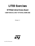
The effect of the interrupt is shown in the following diagram:
A n in te r r u p t is r e q u e s te d
a n d a u th o r iz e d
T h e c u r r e n t in s tr u c tio n is e x e c u te d , th e P C is in c r e m e n te d
T h e P C a n d a s m a ll n u m b e r o f r
a u to m a tic a lly p u s h e d o n to th e s ta
a r e d e fin e d b y h a r d w a r e : a c c u m u
e tc
e g is te r s a r e s a v e d , th e y a r e
c k . T h e r e g is te r s to b e s a v e d
la to r , c o d e c o n d itio n r e g is te r
.
D e p e n d in g o n th e ty p e o f m ic r o c o n tr o lle r , th e lo w e r
p r io r ity o r a ll th e m a s k a b le in te r r u p t s o u r c e s a r e m a s k e d
D o n e
b y
h a rd w a re
T h e P C is lo a d e d w ith th e in te r r u p t v e c to r a d d r e s s w h ic h
is a p o in te r to th e a d d r e s s o f th e in te r r u p t s u b - r o u tin e
T h e s u b - r o u tin e is e x e c u te d a n d e n d s w ith
t h e 'r e t u r n f r o m in t e r r u p t ' in s t r u c t io n
T h e m a s k e d in te r r u p t s o u r c e s a r e a u th o r iz e d
T h e P C a n d p r e d e fin e d r e g is te r s a r e p o p p e d fr o m
T h e n e x t in s tr u c tio n o f th e in te r r u p te d
p r o g r a m is fe tc h e d a n d e x e c u te d
In te r r u p t p r o c e s s in g flo w c h a r t
02-flow
30/315
s ta c k
D o n e
b y h a rd w a re
2 - How does a typical microcontroller work?
2.5.1.1 Hardware mechanism
The hardware mechanism is important to understand. It is different for each product, so what
we shall describe here pertains specifically to the ST7.
An interrupt request is a binary signal (a flag) generated by several external sources. Most peripherals of the ST7 can produce interrupt requests, for example the I/O ports, the timers, the
SPI, the I2C interface, and so on. The external cause of the interrupt request depends on the
type of the peripheral: the I/O ports may have some bits configured to generate an interrupt,
either on low-level, falling edge, rising edge, or both. The timer may request an interrupt on
timer overflow, external capture or output comparison. The SPI may request an interrupt on
end of transmission, etc.
2.5.1.2 Hardware sources of interrupt
The hardware interrupt sources are summarized in the diagram below.
In p u t p in
E x te rn a l s o u rc e
e d g e d e te c t
c ir c u it
e g : p a r a lle l in p u t p o r t p in
In te rn a l s o u rc e
e g : tim e r o v e r flo w
G lo b a l in te r r u p t e n a b le b it
C o n tr o l r e g is te r
o f th e C P U
S ta tu s r e g is te r
o f th e p e r ip h e r a l
In te r r u p t fla g b it
In te r r u p t tr ig g e r
to th e c o re
C o n tr o l r e g is te r
o f th e p e r ip h e r a l
In te r r u p t e n a b le b it
O th e r m a s k a b le
in te r r u p t s o u r c e s
D ia g r a m
N o n m a s k a b le
in te r r u p t s o u r c e s
o f th e in te r r u p t m e c h a n is m
02-mec
31/315
2 - How does a typical microcontroller work?
2.5.1.3 Global interrupt enable bit
The various sources of interrupt may be inhibited as a whole using the I bit in the condition
code register. When this bit is set, no interrupts are generated. However, the interrupt requests are not forgotten; they will be processed as soon as the I bit is reset.
2.5.1.4 Software interrupt instruction
In addition to the hardware sources, a special instruction, TRAP, produces the same effect as
an externally-generated interrupt request, but under program control. Strange as it may seem
(interrupts are provided for handling unexpected events, or at least, events whose time of occurrence is not known), the TRAP instruction utilizes the whole interrupt mechanism within the
regular execution of the main program.
The trap instruction triggers the interrupt processing regardless of the state of the I bit in the
condition code register.
An example of the use of the TRAP instruction is the real-time debugger. When the user sets
a breakpoint somewhere in the program, the debugger replaces the instruction at which the
execution must stop with a TRAP instruction. The interrupt thus generated is processed by
displaying on the screen the state of the microcontroller at that precise time. However, this instruction may be used in other ways as well.
2.5.1.5 Saving the state of the interrupted program
When an interrupt request triggers an interrupt, the first task of the core (after completing the
current instruction), is to save its current state so it will be able to restore it after the interrupt
processing is finished. This is done by pushing all the core registers on the stack. For example, in the ST7, the Program Counter, the X-register, the Accumulator and the Condition
Code Register. It should be noted that the Y register is not saved, (this is because the ST7 has
evolved from an architecture that did not have a Y register). If needed, the Y register should be
pushed explicitly on the stack at the beginning of the interrupt service routine.
To protect the interrupt service routine from being interrupted, the I bit of the Condition Code
Register is set automatically.
At this point, the interrupt service routine may execute whatever instructions the programmer
chooses to write. The status of the interrupted program is known and can be restored when
needed.
2.5.1.6 Interrupt vectorization
When the core decides to grant an interrupt request, it must know the address of the code that
must be executed in such an event. This is the purpose of the interrupt vectors.
The interrupt vectors are a table of 16-bit words in program memory that contain the address
of the beginning of the various interrupt service routines.
32/315
2 - How does a typical microcontroller work?
Depending on the source of the interrupt (I/O, timer, etc.), the core fetches, from a predefined
location in memory, the address of the interrupt service routine especially written to process
that event. The vectors are always located at the end of the addressing space. There is one
vector for each interrupt source, plus one for the reset. When the microcontroller is interrupted
or reset, one of these interrupt vectors is fetched in order to get the start address of either the
interrupt service routine or the start of the main program.
The following table shows the interrupt vectors:
M e m o ry
a d d re s s
L o w e r p r io r ity
F F E 0
n o t u s e d
F F E 4
I²C
B u s In te rfa c e
F F E 6
n o t u s e d
F F E E
T im e r B
F F F 0
n o t u s e d
F F F 2
T im e r A
F F F 4
S e r ia l P e r ip h e r a l
In te rfa c e
F F F 6
n o t u s e d
F F F 8
P o rts B a n d C
F F F A
P o rt A
F F F C
T R A P
S o ftw a re In te rru p t
F F F E
R e s e t v e c to r
H ig h e r p r io r ity
In te r r u p t v e c to r ta b le o f th e S T 7 2 2 5 1
02-tabv
33/315
2 - How does a typical microcontroller work?
2.5.1.7 Interrupt service routine
When the processor has granted an interrupt request, and read the interrupt vector, it starts
executing the interrupt service routine. This routine is merely a segment of program, written
with exactly the same ease and constraints as the main program. It may be written using the
same language and tools, or in any other language.
The interrupt service routine is supposed to take appropriate action according to the source of
the interrupt. For example, if an input bit has changed its state, the service routine may change
the state of an output bit; if the interrupt was generated by the timer, this may produce the
transmission of a byte by the SPI, etc. according to the structure of the application as defined
by the programmer.
Eventually, the service routine is finished. Then the core may return to the main program. This
is done by executing the IRET instruction.
2.5.1.8 Interrupt Return instruction
As described above, an interrupt service routine looks a little bit like a subroutine. Like in a
subroutine, the return address is stored in the stack, and the execution of the RET instruction
returns to the calling program.
However, some more things have to be done before returning to the interrupted program. All
the core registers were pushed on the stack when the the interrupt request was granted (except the Y register). They must now be restored, so that the execution of the service routine
will not leave any trace in the core. This is the role of the IRET instruction in the ST7.
The IRET instruction proceeds by popping all the data off the stack that had previously been
pushed, namely the Condition Code register (at this point the I bit is also restored), the Accumulator, the X register and the Program Counter.
From this time on, execution of the interrupted program resumes.
2.5.2 Software precautions related to interrupt service routines
As described above, the interrupt mechanism is fairly simple to use, since it only consists of
setting the interrupt vectors to the address of the corresponding service routines, and writing
a piece of code that must end with a IRET instruction.
Actually, an interrupt service routine may do anything in the system, since it uses the regular
instruction set of the core and has access to the whole memory. It may thus affect the state of
the main program, even though the core registers have been preserved. The following paragraphs deal with the precautions to take when using interrupts.
2.5.2.1 Saving the Y register
(This point is specific to the ST7.) If the service routine uses the Y register, one must remember that this register is not saved automatically by the interrupt granting mechanism.
34/315
2 - How does a typical microcontroller work?
Thus it is up to the programmer to save it, by pushing it to the stack at the beginning of the
service routine, and popping it before executing the IRET statement.
2.5.2.2 Managing the stack
This is just a reminder, since it applies anywhere in the program. The service routine must
track the usage it makes of the stack, so as to pop at the end as many bytes as it had pushed
at the beginning. This may look trivial, but if some pushes occur in some conditions and not
others (i.e. the service routine has conditional statements somewhere), the popping must
occur in exactly the reverse way, taking into account the same conditions as those that produced the pushing. This may not be very obvious to code.
2.5.2.3 Resetting the hardware interrupt request flags
In some peripherals, the hardware flag that produced the interrupt request is automatically
cleared on servicing the interrupt. In this case, no special care need be taken.
On the contrary, in some other peripherals (such as the timer), the interrupt request flag keeps
its state after the interrupt is granted. This flag must be cleared anywhere in the interrupt
service routine, but necessarily before the I bit of the Condition Code Register is cleared (on
execution of the IRET instruction). Otherwise, the interrupt service routine would be called
again immediately after executing the IRET instruction, and the core would loop indefinitely
through this interrupt service routine, thus blocking the main program.
How to reset the interrupt request flag is described as part of the description of each peripheral.
2.5.2.4 Making an interrupt service routine interruptible
On interrupt granting, the I bit of the Condition Code Register is set, to prevent the service routine being interrupted by incoming interrupt requests. Further interrupt requests will then suffer
from a delay before they are serviced. This delay is called «interrupt latency». Actually this
term includes the reaction time of the core itself, to which the time for the servicing in progress
must be added.
However, there are cases where it is necessary to allow an interrupt service routine to be itself
interrupted. This is the case if a service routine performs processing that takes a certain
amount of time, and another interrupt source requires that its request be processed immediately, i.e. the permitted latency is short.
The solution is then to allow the slow service routine to be interrupted. This may be done by resetting the I bit of the Condition Code Register. This must be done after the hardware interrupt
request flag that triggered the interrupt currently in progress is cleared, for the same reason as
explained above. Please note, however, that this must only be done when necessary, since
the size of the stack is often limited in small microcontrollers.
35/315
2 - How does a typical microcontroller work?
2.5.2.5 Data desynchronization and atomicity
This paragraph addresses the precautions that must be taken, in the main program or any
service routine that may be interrupted.
In many cases, data is organized in blocks in memory, that is, several bytes, successive or
not, make up a piece of data. Some coherence rules must be followed when using these data.
Failure to observe these rules may produce unexpected results and, very likely, an application
crash.
When no interrupts are used, the main program can easily follow these rules by taking care to
perform all data changes in the appropriate order and respecting the predefined relationships
between each of the bytes that constitute a piece of data.
When interrupts are used, respecting the coherence rules may become more complex. Actually, an interrupt is an asynchronous action that can occur at any time. Let us assume that the
main program is currently altering one piece of data that is made of several bytes. It first writes
some bytes, then more bytes until it is finished with a new data in memory.
If an interrupt occurs in the middle of the process of altering the data, the following risk may
appear. If the interrupt service routine uses the data that the main program is writing, the
service routine may get data that fail to follow the coherence rules, since not all bytes have
been updated yet. The service routine may then be misled by an incorrect value that it cannot
handle properly, or just interpret that data differently from what it was expected to mean if it
had been fully modified. This may have very serious consequences on the working of the application. This circumstance is called «data desynchronization».
To avoid this, some precautions may be taken in cases where interrupt service routine may
find incoherent data. They all ensure that all the data will be updated at once, and never used
unless completely updated. This condition is called «atomicity», from a Greek root meaning
«that cannot be cut». To properly handle multi-byte variables that are shared by a main program and an interrupt service routine, or by two interrupt service routines of which one may interrupt the other, the handling must be made “atomic”.
36/315
2 - How does a typical microcontroller work?
The following example shows:
■
What happens when the data are desynchronized.
Let us assume the main program wants to increment the word variable reg (16-bit register in
page zero), that currently contains 42FF hex. The following code will be used:
; word variable reg contains 42FF hex
; increment word variable reg by 1
inc reg+1
; add 1 to the low byte
; low byte is incremented. reg
= 4200 hex
jrne endinc
; increment high byte if carry
endinc : ...
; here the program continues
; both bytes are incremented. reg = 4300 hex
If an interrupt service routines uses the value of reg, and if the interrupt request occurs for example at the first line of the code above, the interrupt service routine will see that reg is 4200
while it is actually either 42FF or 4300. This error may have serious consequences.
■
How to make the handling atomic.
To avoid this situation, it is sufficient to mask out all the interrupts, by changing the code as follows:
; increment word variable X by 1
sim
endinc
inc reg+1
jrne endinc
; prevent interrupts from
occurring
; add 1 to the low byte
; increment high byte if carry
rim
...
; allow interrupts to occur
; here the program continues
; both bytes are incremented. reg = 4300 hex, now the interrupt can be
performed
All interrupt requests that occur between the SIM and the RIM instructions are delayed for the
duration of that piece of code. If this would cause an excessive latency for one particular interrupt that does not use that data, it is possible to mask out the specific interrupt source whose
service routine actually uses this value.
This example mentions the case where the data is written by the main program, and read by
the interrupt service routine. Actually, the reverse case is also a source of problem: if the main
program reads the data, and the interrupt service routine writes it, the main program may start
37/315
2 - How does a typical microcontroller work?
reading the first bytes of the data, then the interrupt occurs; on return, the remainder of the
data are read, but unfortunately there may not be coherence between the first byte that was
read before the interrupt and those read after it.
2.5.3 Conclusion: the benefits of interrupts
The interrupt system is a very appropriate means of processing events that have the following
features:
■
They are triggered by a hardware signal coming from outside. Theses signals are connected
to appropriate pins of the microcontroller; or they are the result of the working of internal
peripherals that reach a certain condition, for example the internal timer has overflowed.
Though the timer is built-in the same chip as the core, it is functionally considered external
to the core.
■
They occur at their own time, and thus unexpectedly for the main program.
■
They require a quick reaction from the core, either because they occur frequently or because
the status of the external device that requests the interrupt would not keep its meaning after
too long a delay.
■
They do not require complex processing; typically, they require reading some data from
outside and storing it to memory, or transferring data from the memory to the external
circuitry.
38/315
2 - How does a typical microcontroller work?
2.6 AN APPLICATION USING INTERRUPTS: A MULTITASKING KERNEL
The conclusion in the previous paragraph states that interrupts are well-suited for a certain
class of events to be processed. However, there are other cases outside this category. Some
of them are better addressed by the concept of multitasking.
In many applications, several processings are required that do not match the specificity of the
interrupt-driven processes. For example:
■
Two or more processes are continuously active, that each take long processing times.
■
These processes are not (or not directly) started by external events.
■
They do not require a quick reaction time.
In such cases, the interrupt concept is obviously inappropriate. Actually, these processes
seem to require each a core of their own. However, considerations of cost may not allow for
multiple microcontrollers on the same board. The concept of multitasking is the answer to this
requirement. It is a software solution that does not require extra components, and makes the
system believe the various tasks run on different cores, although it is simply the same core
that is shared between all the tasks at the expense of the computing power that is shared between this tasks, plus a certain waste produced by the specific mechanisms that provide for
the multitasking. This waste limits the frequency at which the tasks can be switched; if they are
switched too often, the proportion of the time taken to switch tasks becomes too large, and the
corresponding part of the microcontroller computing power is lost. The designer must check
whether the power remaining for each task is sufficient or not; if not, the type of microcontroller
is probably unsuitable for the project.
There are two kinds of multitasking, namely pre-emptive multitasking and non pre-emptive
multitasking. The second kind is also called cooperative multitasking.
2.6.1 Pre-emptive multitasking
Pre-emptive means that the computing power that is allocated to a task is withdrawn from it
without notice, that is, that particular task is stopped at an unexpected place by brute force.
Then, the power is allocated to another task, until it is stopped in turn, and so on for all the
tasks; then, the first task that is currently sleeping regains control and continues for some time.
The task switching is done under control of an interrupt triggered by a timer. This allows the
core time to be partitioned at will between the various tasks. The time for which each task is allowed to run may be the same for all tasks; or it may be decided to allow more time for some
more important (or time-consuming) tasks, and less for others. In a word, the multitasking
kernel may fine-tune the resource sharing between the tasks.
The main drawback of this system is that since the tasks are interrupted at any place in the
code, many precautions must be taken to ensure the coherence of the data, just as explained
above about interrupts. In fact, if a task starts to write a piece of data and is put asleep in the
39/315
2 - How does a typical microcontroller work?
process of updating the data, and another task uses that data, there is a risk of desynchronization. The same type of precautions must be taken to ensure atomicity of data updates. The
same problem may also occur if more than one task handles control sequences for an external
device. If this external device needs a precise control sequence that must be completed before a new sequence is started, there is a risk that a task may lose control before the sequence
is complete and control may be transferred to a task that attempts to use the same device. The
attempt may then fail or interfere with the unfinished sequence of the previous task. Here
again, a protection mechanism is required.
In summary, the advantage of pre-emptive multitasking is that task switching is done automatically and independently from the code of each task; the relative power attributed to each task
may be adjusted to fit the requirements of each task.
The drawback is the opposite of the advantage: since the task switching happens at any time
and any place in the code, the programmer must locate the critical areas of code where special protection mechanisms must be included. This may be more difficult than it might appear,
for it is not always easy to find all the possible collisions and keep them from happening.
F ir s t ta s k
T im e
A n a llo tte d tim e
is a s s ig n e d
F o u rth ta s k
to e a c h ta s k
T h ir d ta s k
P r e e m p tiv e m u ltita s k in g
02-preem
40/315
S e c o n d ta s k
2 - How does a typical microcontroller work?
2.6.2 Cooperative multitasking
Cooperative multitasking draws its name from the fact that task switching is not spontaneous.
It only occurs when the task-switching function is called by the currently active task. This implies two facts:
■
Task switching occurs only when the code decides it. As a consequence, it is easy to avoid
data desynchronization and access collisions by placing the task switching calls at the
proper places.
■
The partitioning of the core time between tasks cannot be set at will, since it is not possible
either to insert into the code as many calls to the switching function as necessary or to put
them at the right places to control the time intervals allocated to that task.
The reader can easily see that the strong and the weak points of one type of multitasking are
the opposite to those of the other system. This explains why both are used, the type being
chosen to best match the application’s requirements. In addition to theses features it is fair to
say that cooperative multitasking is easier to implement and less resource-consuming than its
competitor.
T a s k 2
T a s k 1
T a s k 3
N e x t ta s k
( Y ie ld )
N e x t ta s k
( Y ie ld )
N e x t ta s k
( Y ie ld )
C o o p e r a tiv e m u ltita s k in g ; s im p lifie d e x a m p le
02-coop
41/315
2 - How does a typical microcontroller work?
2.6.3 Multitasking kernels
2.6.3.1 Advantages of programming with a multitasking kernel
The multitasking kernel is the piece of code that controls the multitasking. The way it does it,
and the flexibility it offers may vary greatly from one kernel to the other. It is generally supplied
ready made, and the programmer has to give his program the appropriate architecture to get
the benefits of it.
Writing an application with multitasking in mind is easy and leads to a clear, organized structure. The work to do is divided in tasks, and these tasks are written separately as procedures.
They exchange data using either communication mechanisms built-in to the kernel, or
common data in memory, taking care to avoid collisions. The main difficulty is to identify what
a task actually is. For example, two processings that are always performed one after the other,
and always in the same order, constitute a single task. On the contrary, two processings that
either may or must be performed at the same time are two separate tasks.
The features of a kernel vary from product to product. One must first know which kernel is
being used, the type of multitasking (pre-emptive or cooperative), and the services provided
by the kernel. Some of these are discussed below.
2.6.3.2 The task declaration and allocation
The kernel must be aware of the existence of the tasks, their number and their start addresses. Some kernels expect this to be stated at compile time; in this case, the number of
tasks is known from the beginning of program execution and cannot change afterwards.
Some others allow tasks to be added (or created) while the program is running. This allows
tasks to be created when the need shows up, for example to process an incoming event and
then terminate. In this case, it is convenient to also have the ability to remove or kill the task.
Again, there are two options: a task may terminate when it decides to do so (kill itself or “suicide”); or it may be killed by any task, including itself.
2.6.3.3 Task sleeping and waking-up
A task may be alive but have nothing to do; in this case, to save computing power, it is wise to
completely stop allocating core time to it. The task is then asleep. This can be done by calling
a function often called Sleep, passing to it the identification of the task to be put asleep. A task
can put itself asleep if it is waiting for some event.
Obviously, it is necessary to have a means of waking-up a sleeping task. This cannot of
course be done by the sleeping task itself, and can only be done either by other tasks or by an
interrupt service routine. For example, let us consider a task that processes the keystrokes
generated by a keypad. The hardware of the keypad may generate an interrupt when a key is
pressed. This interrupt may wake-up the keypad task that reads the keycode and takes the
appropriate action. When this is done, the task may go asleep again. One might ask why it is
42/315
2 - How does a typical microcontroller work?
not simpler to perform the processing right in the interrupt service routine, instead of this apparent complexity. Actually, the processing of the keystroke can take a long time, too long to
allow it to freeze the remainder of the application as happens when an interrupt is being serviced.
Other services may be supplied by the multitasking kernel, coping with priorities, intertask
communication, etc.
2.6.3.4 Multitasking kernel overhead
The purpose of a multitasking kernel is to share the power of a single processor or core between several tasks. Obviously this sharing means less power for each task, except perhaps
if all tasks but one are asleep. However, even in that case, the task does not benefit from the
whole computing power, since some of the core power is drawn off by the kernel itself. In addition, it is equally obvious that the kernel is a piece of code that occupies a certain amount of
program memory as well as data memory. But overall, the main concern with memory requirements relates to the stack.
The stack is the place where the state of a program is continuously stored. This amount of
data is often referred to as the “context”. Each task has its own context, which consists of all
the return addresses of all nested procedures and functions; most compilers also store the
function arguments and local data in the stack. This can add up to a large amount of memory,
not to mention that some free space must remain in the stack to handle interrupts that may
themselves consume a certain amount of stack, in the same way as the main program.
This implies generally that the stack space must be very large, since the amount of data mentioned above must be multiplied by the number of tasks alive at the same time.
The ST7, being a small 8-bit core, provides for at most 256 bytes of stack. This allows for a
multitasking kernel with a limited number of tasks and services.
43/315
2 - How does a typical microcontroller work?
C o m m o n p a rts
o f th e p ro g ra m
S ta c k
p o in te r
C o d e o f th e
fir s t ta s k
S ta c k a re a
fo r ta s k # 1
1
2
S ta c k a re a
fo r ta s k # 2
3
C o d e o f th e
s e c o n d ta s k
4
S ta c k a re a
fo r th e la s t ta s k
C o d e o f th e
la s t ta s k
S ta c k R A M
In te rru p t v e c to r
ta b le
P ro g ra m
m e m o ry
1
S e le c tio n o f th e ta s k : T h e s ta c k p o in te r p o in ts to
th e la s t d a ta o f th e ta s k to a c tiv a te th a t is s to r e d
in th e s ta c k .
2
A c tiv a tio n o f th e ta s k : T h e p o p p in g o f th e d a ta o ff
th e s ta c k r e s to r e s th e ta s k s a s it w a s b e fo r e b e in g
u n s e le c te d .
3
4
D e s e le c tio n o f th e c u r r e n t ta s k : T h e s ta te o f th e p r o g r a m is s a v e d in th e s ta c k b e fo r e it is d e s e le c te d .
S e le c tio n o f th e fo llo w in g ta s k : T h e s ta c k p o in te r
p o in ts to th e la s t d a ta s a v e d fr o m th e n e x t ta s k s
to a c tiv a te .
W o r k in g m e c h a n is m
o f a s im p lifie d m u ltita s k in g k e r n e l
02-task
44/315
3 - Programming a microcontroller
3 PROGRAMMING A MICROCONTROLLER
A microcontroller is basically a programmable component. This means that it can do almost
anything, when properly programmed.
In fact, the design of the electrical schematic of a microcontroller-based application raises few
questions; the input and output pins of the microcontroller are simply connected to the binary
signals either produced or used by the external application. The designer only has to take care
to select the right pins, since some signals must be connected to special peripherals like the
Analog to Digital Converter, the Timer, etc.
It is the program that configures the pins so that they have the correct electrical behaviour, and
that processes the data to produce the appropriate response to the input signals. Since the
board will be designed with as little electronic processing as possible, all the processing is
done by software.
This produces the flexibility that is the main feature of any programmed system: unless a hardware problem arises, most of the fixes and changes done to a programmed system will be
done in software.
Programming the processor is thus the key activity of the designer, the one that will take the
largest part of his time. For this reason, the use of the right tool to program the application is
critical, since program design and testing time can vary greatly according to the tools and the
language chosen.
This chapter addresses the two main issues the programmer faces: selecting the appropriate
language for the best productivity, then selecting the appropriate software tools that will allow
not only to program in that language, but also to test the program written in that language. We
will learn that an investment made prior to starting the design can prove very efficient in terms
of development time, and therefore, pay for itself.
3.1 ASSEMBLY LANGUAGE
3.1.1 When to use assembly language
Assembly language is the native language of each microprocessor. It used to be the only way
of programming a small microcontroller until high-level language compilers were made available. Programming in assembler was a job that required a lot of care and very many lines of
source code relative to the size of the application. It was justified when program memory was
small and assembly language was the only way to optimize the code size. Nowadays, microcontrollers, except for those at the lowest-end, can afford enough memory to cope with the
code expansion factor inherent in high-level languages. Thus, for reasons explained in the following paragraph, a high-level language is strongly recommended and using assembly language should not be considered except when absolutely needed.
45/315
3 - Programming a microcontroller
There are, in almost all applications, parts of the code that still require assembly programming.
These parts are, most of the time, small but have an important impact on the program. Here
are a few such cases:
■
The initialization part of the program. All high-level languages provide for initialization of the
core and the memory. However, the basic organisation of the memory (address of the ROM
and the RAM, reset and interrupt vectors) and a few other kinds of initialization are supplied
as an assembly-language template, that has to be adapted to suit the actual application.
■
Some interrupt service routines that require very fast processing.
■
Some repetitive functions that are frequently invoked and whose optimization in terms of
speed has an important impact on the performance of the whole program.
The third case implies that the programmer carefully reads the implementation chapter of his
compiler’s manual. The way arguments and return values are passed back and forth are specific to each compiler. Failure to comply with these conventions will prevent the assembly
code from working.
3.1.2 Development process in assembly language
The development of a program consists of three main phases: analyzing, writing the code, debugging. In other words, the successive phases can be described as follows:
■
The first phase is when the programmer defines what the program should do. This is only
paperwork, even if it is done using a computer and a word processor or a spreadsheet. This
phase defines the main program blocks, the data inputs and outputs, the storage, and some
of the algorithms.
■
The second phase is the translation of the first one into the chosen computer language. The
result of it is the source code and a few files that drive the various programming tools. The
tools used in this phase are the text editor, to type and amend the source code, and the
assembler and the linker to check its syntactic correctness. The Make utility is also a
convenient tool, that helps keeping the program up-to-date, when any of its parts have been
changed, by processing only the changed source files.
■
The third phase consists of all that is needed to make the source code work. It involves
removing all programming errors, that is, the flaws in the first and second phases related to
logic, coordination, and data management. This third phase is by far the most difficult and
requires the most development time. The tools used, the Simulator and In-Circuit Emulator,
have to be very powerful because many errors are difficult to find.
When the program is fully functional, it is often stored in an EPROM that is either external, or
as in the ST7, internal to the microcontroller. This produces a prototype of the microcontroller
that must be extensively tested before being launched to production, especially if, for large
46/315
3 - Programming a microcontroller
quantity production, the microcontroller includes a masked ROM programmed by the device
manufacturer and that cannot be altered afterwards.
3.1.2.1 Assembly language
Assembly language is merely a set of mnemonics that duplicates each instruction in a more
legible way, to help writing the programs. Machine language is just a series of numbers that
obeys a certain code to indicate to the core which instruction to execute and which data to use.
Assembly language provides acronyms that are easier to remember. The following example
shows an excerpt from an assembly listing. The first two columns show numeric data, which
represent the addresses of the instructions and the machine-language code. The Source line
column shows the machine code in mnemonic language. It is obvious that, provided one has
learned that ld means the instruction Load, and that, of the two operands of this instruction,
the destination operand comes first, it is easy to understand the first lines of source code as
documented in the comment column:
Loc
Obj. code
------ --------000000 A6FF
000002 AE64
000004 F7
000005 5A
000006 26FC
Source line
----------ld A, #$FF
Comment
------------; load accumulator with immediate
data FF (hex)
ld X, #100
; load X register with value 100
loop: ld (X), A
; load location pointed to by X
with contents of A
dec X
; decrement X register
jrne loop
; jump to label loop if X not equal
to zero
This short program is a loop that fills memory addresses 100 to 1 (decimal) inclusive with the
value FF hex.
Programming in assembly language involves using a text editor to write a text file that obeys
the syntax and conventions of the specific assembler that is to be used. It should be noted that
assembly language is not standardized in any way, for two reasons:
■
The instruction set changes from one processor to another
■
For a specific processor or microcontroller, software tool sets from different suppliers each
have their own syntax, although two source files written for two different tool sets may seem
very close.
Thus, to write an assembly language source file, the programmer must first know which processor or microcontroller will be chosen for his project, then which software tool set he will use.
Then, he has to learn both the characteristics of the processor’s instruction set (instruction
types, addressing modes, etc.) and the specific syntax of the assembler he will use.
47/315
3 - Programming a microcontroller
Then, once he masters both, he may start to write his source file. Obviously, if later he has to
do the same job with a different processor, the source file will be of no use in the future project.
3.1.2.2 Assembler
The word assembler has usually two meanings. Properly used, it is a program that translates
a text file, written according certain rules, into a binary file that contains a series of instructions
specific to a microprocessor or a microcontroller. However, the word Assembler is often improperly used instead of “assembly language”, for example in the sentence: “this program is
written in assembler”. This paragraph introduces the translating tool, or “assembler”.
The assembler is a program that runs on whatever computer is used by the programmer for
his regular job. It takes the source file, as explained above, as an input; then, after translation,
it outputs, depending on the user-specifed options, any of the following files:
■
The object file, containing binary data intended for further processing. It can not be read by
man.
■
The listing file, is a report containing both the original source code and its numeric
translation, presented in a tabulated manner. It can be read by man and used for reference
purposes.
■
In some cases, other files like lists of variables and labels, or additional data. This varies
from one assembler to another.
If the assembler encounters an error in the syntax of the source file, or some ambiguity or lack
of information preventing it from completely processing the source file, it generates an error
report, this may be output in the listing, in a separate file, or directly on the computer console.
The error messages tell where the error is located, and, as much as possible, the cause of the
error, as in the following example:
TRIAL.ASM(6): ERROR: not a ST7 instruction or directive
48/315
3 - Programming a microcontroller
Here again, the format of all the above mentioned files is chosen by the assembler’s manufacturer, and differs from one to another.
F ile .o b j
F ile .a s m
A s s e m b le r
R e lo c a ta b le o b je c t file
F ile .ls t
S o u r c e file
L is tin g file
A s s e m b le r in v o c a tio n
03-asm
3.1.2.3 Linker
If the whole application program is small, it is easy to put the source text into a single file. The
assembler then produces an object file that contains the whole machine code ready for use.
This is called absolute assembling.
However, there are very few applications so simple that their source text occupies only a few
pages. In most cases, the total source text amounts to thousands of lines that may represent
hundreds of pages. In such a case, it would be impractical to edit a single large source file. Not
only would the assembly process take a long time but this time would be spent whenever a
change was made to the text.
It would be better to divide the whole text into several files, and to assemble them separately.
This way, a change would affect only one of the files, which can be quickly re-assembled.
Working this way requires additional features:
■
A means of telling that a particular source file references a data variable or a label that is
defined in another source file, in order to prevent the assembler from merely stopping and
issuing an error message saying that something referred to has not been found defined in
the same source file.
■
A tool to glue all the generated object files into a single object file, ready for use.
The first issue is addressed by additional syntax features that typically provide declarative
statements such as “External” and “Public”. The “External” statement declares that a certain
label referenced in the source file will intentionally not be found there, since it comes from another source file. The “Public” statement declares that a label (or a variable) defined in this file
will be referenced by another source file.
49/315
3 - Programming a microcontroller
The tool that glues together all the object files, each the result of assembling the source files,
is called the Linker.
The linker performs the following tasks:
■
It takes all the object files, and merges them into a single object file by concatenating them
one after the other.
■
It corrects the address values in all the instruction operands that refer to objects whose
location in memory has been set or altered by the concatenation.
To do this, in addition to the set of object files, the linker requires a control file that tells it the
list of the object files to link together, the order in which they must be put, and the absolute addresses at which the result will be installed in the microcontroller’s memory.
This may look complex; but actually, it make processing large programs easier and faster.
When a change has to be made to a particular source file, only this file must be edited. Then
only this one must be re-assembled, which saves time; then, all the object files must be linked
again. The linking process is fast, compared to assembly, since the files contain binary data
and their format is optimized to make the linker’s job easier.
If a hardware change is made to the board that changes the address of some memory or a peripheral, it may be only necessary to alter the linker control file and link the program again.
Once the program is linked, the resulting object file contains the whole program. This file is
said to be an absolute object file, meaning that all addresses are defined; as distinct from object files before the link process that are said to be relocatable, i.e. their addresses can be
changed later.
The absolute object file can be used either to be downloaded into an emulator to check and
debug the program; or into an EPROM programmer to program the chip that will hold the
code.
As for the assembler, the linker is built to process relocatable files produced by the assembler
frim the same tool set. It is usually not possible to mix the tools, like assembling with the assembler from supplier A then linking with the linker from supplier B.
50/315
3 - Programming a microcontroller
F ile .c o d
o r
F ile .a b s
F ile 1 .o b j
A b s o lu te o b je c t file
L in k e r
F ile 2 .o b j
F ile .s y m
S y m b o l ta b le
F ile 3 .o b j
F ile .m a p
R e lo c a ta b le o b je c t file s
M a p file
L in k e r in v o c a tio n
03-link
3.1.2.4 The project builder/make utility
In the process introduced above, that relies on splitting-up the processing to save time, it is important to keep track of which sources have been altered, only re-assemble these and not the
others and then link all the object files. Forgetting to do this may waste a lot of time. For example, after making a correction, if a program still shows the same incorrect behavior as previously, one is tempted to suspect another part of the code. Trying to identify which other part
of the program produced the problem will be a useless effort, if the real reason was that the file
containing the change had not been re-assembled and linked.
Thus, a tool that can guarantee that the programmer will never forget to reprocess his files is
an invaluable help. This tool is called Maker or Make utility.
The maker is a tool that works under the control of a file that gives the names of the source
files, the name of the output object file, the names of the tools needed to process a file to another file (assembler, linker), and the dependency relationships between the files.
For example, the dependency relationships specify that the final object file is produced by applying the linker tool to the files named in the linker control file; that each of the individual object files is produced by applying the assembler tool to the corresponding source file, etc.
The maker works as follows:
51/315
3 - Programming a microcontroller
Each time a file has a successor with a date older than its predecessor, the corresponding tool
is run to update the successor. This is done in an orderly fashion, from the top of the hierarchy
(the source files) to the bottom (the absolute object file). Then, at a given time, all those source
files that have been modified since the last run of the maker are reprocessed, and only those
files. This both guarantees that no file will be forgotten in the updating process (provided that
the control file correctly describes all the dependencies), and that only the necessary
processing will be done, to save time.
The maker is an essential component of any set of programming tools. But unlike what was
said about matching the same brand of assembler and linker, any maker may be used in a
project, since all work the same way. The control file, in fact, uses a different syntax; but this
does not affect the overall result. So, if you buy a new set of software tools for a microcontroller, you can still keep the maker you are accustomed to.
3.1.2.5 EPROM burners
EPROM burners, or programmers, are tools that have a hardware interface with a zero-insertion force socket that matches the characteristics of the specific EPROM chip or microcontroller with built-in EPROM. They transfer the contents of an absolute object file into the physical programmable memory. Burner software usually accepts several input formats. This gives
some flexibility to the user and can allow using a burner from one manufacturer with software
tools from another. Apart from accepting absolute object files generated by the linker in the
same tool set, burners also frequently accept one or other of the more widely-used printable
hexadecimal formats.
To use a hexadecimal format, either the linker must be able to output an absolute file in that
format, or a code converter must be used that takes an absolute object file as an input, and
produces a hexadecimal file as an output. Such converters are often supplied with in the software tool set. The use of these converters may save you the price of a new burner if you already own one for the right type of programmable component.
52/315
3 - Programming a microcontroller
F ile .c o d
o r
F ile .a b s
A b s o lu te o b je c t file
E x e c u ta b le file
F ile .s 1 9
E p ro m
p ro g ra m m e r
fo rm a tte r
M e m o ry c o n te n t
im a g e file
m ic r o c o n tr o lle r
w ith b u ilt- in E P R O M
P r o g r a m m in g a m ic r o c o n tr o lle r
03-prom
3.1.2.6 Simulators
A simulator is a tool that pretends to run an absolute executable program. Like the other tools,
it runs on the programmer’s own PC. It interprets the machine code that is specific to the
chosen processor or microcontroller, and outputs the results on the PC screen, without the
need for actually building the application hardware or even obtaining a sample of the target microcontroller.
The simulator allows the program to be run step-by-step (instruction-by-instruction), allowing
the programmer to watch the values changing in any register or memory location that result
from the execution of the instructions. It also makes it possible to put breakpoints in the program, which are traps that stop the execution it reaches the address of the instruction where
the breakpoint was put. This can be used to run some parts at full speed and then stop on
reaching parts that are not yet fully functional, to avoid walking step-by-step through a lot of instructions that have already proven to be correct.
The progress of the execution can be followed on the screen in a special window that shows
the source file, and a cursor indicating the next line to be executed. At the same time, other
windows may display items like a range of data memory, the registers, the values of selected
data in a selected format (byte, word, character string...).
The user is even allowed to alter the values of the registers of the core, of the input-outputs, or
in memory, for example to correct a programming mistake, and continue the execution with
53/315
3 - Programming a microcontroller
the correct values, so as to avoid having to edit and make the program each time an error is
found.
In fact, simulation is limited to pieces of code that do not access the input-outputs, since this
would require a complex program at simulator level to also simulate the behaviour of the external world that the application is supposed to interact with. But still, most simulators can correctly emulate the operation of the built-in peripherals, in particular the programmable timers,
and can trigger interrupts whose servicing can be monitored on screen.
Simulation, though limited in its possibilities, has the advantage that it allows to you start debugging the application program before the hardware becomes available,. It can speed up the
debugging process by ensuring that some pieces of code are already functional when the time
comes to test and debug the hardware.
3.1.2.7 In-circuit emulators
In-circuit emulators are complex and expensive instruments that, for the application hardware,
behave exactly like the intended microcontroller would do. From the user’s point of view, an
emulator is an inspection device that shows the calculations in progress in the application
hardware and the state of the input-outputs, as well as the contents of the memory at any time.
It is the electronic equivalent of a spy in the real world: an intermediate entity that, while
playing its role correctly in the real world (the application hardware), at the same time informs
an external intelligence (the programmer) of everything that happens in that world.
An emulator offers exactly the same features as a simulator does, in terms of running an application either at full speed or step-by-step, setting breakpoints, examining registers, memory
and input-outputs. The major difference is that while running the program, the microcontroller
actually interacts with the external world, producing actions on the product to be tested, and
acquiring real data that it can process in a realistic way.
The simulator and the emulator are so close together in functionality that the manufacturer endeavours to provide the same user interface, i.e. the same presentation on the screen and the
same controls through the keyboard and the mouse for both tools, so that the user has very
little additional learning to do when switching from the simulator to the emulator.
One last feature that is found on top-range emulators (the very expensive ones) is so-called
real-time tracing. This is a hardware system that records all events on the buses (address,
control and data) and attaches a time tag to them. The memory capacity is at least one thousand events, and can exceed ten thousand in the most expensive emulators. This allows you
to run the program at full speed, record what is going on, then quietly analyze the record to see
what happened. In real-time applications, this may be the only way to understand what happens and the problems that occur, as most of these applications do not permit step-by-step
debugging, since the processor must follow the activities of the external world in real-time. In
54/315
3 - Programming a microcontroller
this type of situation, its a difficult task for the programmer to complete the debugging of the
application so that it can be validated.
3.2 C LANGUAGE
3.2.1 Why use C?
Many high-level language exist; some have been written specifically for a family of microcontrollers, while others are widely-used languages from the computer world that have been
adapted to suit the needs of microcontrollers. Today, one language that prevails in microcontroller programming, that is C language.
The primary advantage of C is the ability to write very simple statements that actually involve
hundreds of machine instructions. As an example, the small sample of assembly source code
given in the paragraph about the assembly language has five lines. It could be replaced by the
following line:
memset ( (void*)1, 0xFF, 100 ) ;
This example is not very impressive. However, a C-language statement like:
int UnitPrice, Quantity, Cost ;
float Discount ;
void main ()
{
Cost = (float)( UnitPrice * Quantity ) * ( 1 - Discount ) ;
}
is easy to read and translates into about eighty instructions, without taking into account the
subroutines that perform multiplication and subtraction. We can see at a glance the productivity gain we can expect from a high-level language.
C language was initially designed as the programming language that came along with the
UNIX operating system. The power and relative simplicity of it made it spread to many different cores, until it became the standard programming language for microcontrollers.
The advantage of C is that it is a language that, though being very powerful, remains very
close to the hardware. This is a key feature for microcontroller applications, especially where
parts of the code are written in assembler. Being close to the hardware means the ability for
the compiler to produce very optimized code by choosing the best instructions for a given job,
when several instructions are available. In particular, setting a port pin high or low must not
55/315
3 - Programming a microcontroller
take a long string of instructions, since the designer of the microcontroller has worked hard to
provide efficient instructions to do the job.
C is a structured language, meaning that code can easily be divided into blocks that can
readily become functions, or the body of looping or conditional statements, keeping the source
code legible if the writer has taken some precautions in the layout of the source text and provided useful comments.
Saying that C is a powerful language means that a short statement, taking only a single line of
source text, may perform complex operations, involving hundreds or thousands of basic instructions. Not only does this conciseness help keep the source text easy to read, but also it
guarantees the correct execution of the code it hides, since this code has already been extensively tested by the manufacturer of the compiler.
The availability of C on many computers makes it possible for you write and test some parts of
the program directly on your PC. Most of the time, if the language constraints have been adhered to, a piece of code that works on a PC will work straight off on the target microcontroller.
This is a recommended method of development, since it allows you to start writing and testing
the program before the hardware of the application has actually been built. The less debugging is done directly on the hardware, the quicker the development takes.
The portability of C is also a guarantee for the future. The microcomputer world evolves so
fast, that it is not unusal to have to redesign an existing application for another microcontroller,
or to reuse parts of the code of a previous application for a future one. In such an event, the C
language allows you to reuse code with virtually no change from project to project. This feature alone, pays back the moderate investment the C compiler represents.
To remove any doubts you might have about the sincerity of these arguments and since
nothing is perfect, the drawbacks of C are be listed here.
The first drawback is that C was originally designed for mainframe computers. In these machines, there is only one memory space, that contains both code and data. In the ST7, there
is also a single memory space that contains code, data and input-outputs, but the code resides in ROM and data in RAM. Standard C has no provision for specifying the address
ranges of these parts of memory.
The interrupt service routines may, and if possible, should be written in C, like any other part
of the code. However, standard C does not know anything about interrupts.
Inputs and outputs are handled in a mainframe through the operating system. Thus standard
C has no special provision for handling them.
These drawbacks would totally prevent you from using C for microcontroller appilactions if the
various implementations of C available did not provide solutions for these cases. These solutions vary from implementation to implementation, and constitute the main cause of non-port-
56/315
3 - Programming a microcontroller
ability of programs to another machine. You will have to take account of this, especially when
testing the code on your PC first as suggested above. This can in most cases be solved by a
declaration file that is included in the project and that exists in two versions, or uses conditional compilation, to fill the gap between two different dialects of C. This point is actually the
most tricky and that which requires most care from the programmer.
Having read these pros and cons, you have hopefully concluded that C is the language of
choice for today if you want to save time and keep the fruit of your efforts over several years.
We have kept the last argument for the conclusion, that will, undoubtedly, be decisive in the
years to come.
The pressure for quality products is growing more every day. In some types of application, like
medical apparatus and life-sustaining devices, equipment reliability has to be certified. More
and more products, through ISO9000 standards or the constraints of product liability must be
ready for quality assurance certification. Software quality assurance is a very difficult subject;
it is not the purpose of this book to enter this field. But one thing is sure, only properly documented and structured software is likely to meet these quality assurance requirements.
3.2.2 Tools used with C language
Just like the assembler translates mnemonic language into machine code, the C compiler is a
tool that translates a C-language source file into a relocatable object file. Here also, the application will be divided into files, also called modules, that are compiled separately. The whole
group of object files is then linked to produce an absolute object file, the same as with assembler-generated object files. Actually, there is virtually no difference between an assemblergenerated object file and one generated by a C compiler. This means that some modules may
be written in C, and some in assembler; you can select the language according to the advantages and drawbacks of each language for each part of the application, as explained earlier.
57/315
3 - Programming a microcontroller
C
F ile .c
F ile .o b j
c o m p ile r
C s o u r c e file
R e lo c a ta b le o b je c t file
(o n s o m e
F ile .a s m
c o m p ile r s )
A s s e m b le r s o u r c e file
C c o m p ile r in v o c a tio n
03-comp
3.2.3 Debugging in C
Debugging in C is done the same way as explained for assembly language. However, the simulator and debugger screens designed for high-level languages can also show the progress of
the execution directly in the C-language source text, while another window shows the corresponding assembly language statements. A cursor in each window keep the correspondence
between both.
Another powerful feature offered by high-level language debuggers is the capability of displaying the data of selected variables according to their type, even for complex types like
structures, arrays, strings, etc. This dramatically improves the productivity of the debugging
phase, in the same proportion as choosing a high-level language does, in terms of shrinking
the source code.
Thus the advantage of high-level languages is twofold: it reduces both the programming time
and the debugging time. This is an invaluable benefit, as the resource that is probably the
scarcest nowadays is time, even more than money. However, you are advised to check
whether of the programming tools you selected fully support C language from one end to the
other; just to mention a few essentials:
■
A text-editor that provides features that are useful in C language, like auto-indenting,
bracketed block selection, syntax highlighting, and so on;
■
A compiler, an assembler and a linker that are really suited to working with the selected
microcontroller, offering flexible addressable space allocation, efficient access to the ports,
58/315
3 - Programming a microcontroller
easy interrupt declaration and servicing in both assember and C language; efficient
optimization that may be switched off at critical places;
■
A simulator and a debugger that properly display the C source text, allowing you to easily
change the values of variables or even code in memory to make patches, and that correctly
synchronizes the timers during step-by-step execution.
These are just a few of the features that may make the difference between apparently equivalent competing products.
59/315
3 - Programming a microcontroller
3.3 DEVELOPMENT CHAIN SUMMARY
The development chain discussed above can be understood more clearly using a diagram.
The diagram below shows the various files involved in the development process as cylinders;
the translators used to change one file type into another are shown as rectangles.
C s o u r c e file s
R e lo c a ta b le
o b je c t file s
M a in
p ro g ra m
C o m p ilin g , a s s e m b lin g a n d
lin k in g in s tr u c tio n s c a n b e
w r itte n in a m a k e u t ilit y file
in c lu d e file s
C m o d u le
# 1
in c lu d e file s
A s s e m b le r
s o u r c e file s
T o th e
p ro g ra
o r th e
fo r s im
o r in - c
e m u la
A b s o lu te
o b je c t file
C c o m p ile r
R O M
e r
u g g e r
tio n
it
A s s e m b le r
A s s e m b le r
m o d u le
# 1
( 1 ) L in k e r
p a r a m e te r file
(1 )
d e v
th is
th e
p ro
file
file
in c lu d e file s
A s s e m b le r
m o d u le
# 2
D e p e n d in g o n th e
e lo p m e n t to o ls c h a in ,
file w h ic h c o n ta in s
m e m o ry m a p o f th e
je c t, c a n b e a s o u r c e
in s te a d o f a p a r a m e te r
fo r th e lin k e r
L in k e r
T y p ic a l s o ftw a r e d e v e lo p m e n t to o l c h a in
03-tchai
60/315
E P
m m
d e b
u la
ir c u
tio n
3 - Programming a microcontroller
3.4 APPLICATION BUILDERS
An application builder is a graphical language that allows you to define the function of the program by manipulating icons on a computer screen. Each icon represents a standard function,
like addition, integration, comparison, etc. Each icon has inputs and outputs, and by drawing
lines on the screen between the output of one icon and the input of another, you connect these
icons, that is, feed one program block with the output of the previous program block. This kind
of programming tool is becoming popular in laboratory and plant automation since it allows
you to build a complete application without leaving the block diagram conceptual level. This
makes it a quick and easy-to-use programming tool for non-programmers.
An application builder for the ST6 and the ST7, the STRealizer, allows you to use graphical
input techniques and build programs based on functional block diagrams. Version 2.2 of the
STRealizer is available on the ST7 CD-ROM.
3.5 FUZZY-LOGIC COMPILERS
Fuzzy logic is a mathematical theory that has been applied to cope with problems that are at
the border between logical and analog computation. It has lead to many articles and books to
explain both its basic theory and various methods of implementing it using microprocessors.
Although it is a very attractive theory, there is no evidence so far of a typical application domain, though quite a few claims have been made about robots, washing machines and
vacuum cleaners, that have been said to be able to adapt their operation to the job they have
to do. One example was a washing machine able to determine the proper amount of water
needed for a certain weight of clothes--without using a scale to measure the weight.
Several fuzzy-logic compilers are available today, in particular one for the ST6 family, however there is none yet for the ST7.
61/315
4 - Architecture of the ST7 core
4 ARCHITECTURE OF THE ST7 CORE
4.1 POSITION OF THE ST7 WITHIN THE ST MCU FAMILY
The STMicroelectronics range of microcontrollers is very wide, from proprietary architectures
like ST6 to ST10 to second-source products like microprocessors for PCs and Digital Signal
Processors.
The proprietary range can be summarized as follows:
Type
ST6
Word size
8 bits
Main features
Very low power consumption, 1.2 to 8
KB ROM,
timer, ADC, watchdog timer and more
depending on the subtype.
Typical applications
Appliances, home automation (suitable
for direct power line supply)
8 bits
Industry-standard instruction set, 256 to
3K bytes RAM, 4 to 60 KB ROM, ADC,
SPI, 16-bit timer, and more depending
on the subtype.
TV remote control, car radio control,
RDS decoder, etc.
ST9
8/16 bits
250 ns instructions (on a 16-bit word),
many internal registers, powerful addressing modes, interrupt priority controller, DMA controller, plus a whole
range of peripherals capable of complex
processing. 16 to 128 KB ROM, more
than 256 bytes RAM.
Automotive body applications and car
radio.
ST10
16 bits
100 ns instructions (on a 16-bit word), 72
KB Flash EPROM, 10+ KB RAM, ADC,
16-bit timer, USART, and more.
ST7
Engine management systems, air bags,
etc.
As the table shows, the ST7 is positioned towards the low-end. It provides an economical
trade-off between speed and price and is suitable where moderate computational power is
needed together with a low-consumption device, like in TV remote control transmitters.
Alhough it is a low-end product, because the ST7 combines the world’s best-selling 8-bit instruction set with a host of added functions from a range of smart peripheral blocks, it is remarkably versatile for a microcontroller of its class. It has a wide choice of versions in order to
minimize the component count of each specific application.
62/315
4 - Architecture of the ST7 core
4.2 ST7 CORE
The ST7 core uses an extended version of an industry-standard instruction set. This set is
both exhaustive (almost all instructions are available, with the exception of division) and fairly
orthogonal (the instructions allow for most addressing modes). This makes the instruction set
of the ST7 both clear and easy to use when programming in assembler.
For those of you already familiar with the standard instruction set, the extension resides
mainly in the following two points:
■
A second index register, Y, that can be used anywhere the X register is used (like indexed
addressing), or like X, moved to any other register;
■
The indirect addressing modes, that come in addition to the direct, long, and indexed modes.
The core as described here is limited to the processing unit, excluding the reset and interrupt
circuitry. They will be described in the chapter dealing with the peripherals. The block diagram
of the core and the addressing space is shown below:
63/315
4 - Architecture of the ST7 core
C P U
C o n tro l
C o re
C P U
A c c u m u la to r
A r ith m e tic
a n d lo g ic
u n it
R e s e t
Y in d e x r e g is te r
C lo c k
X in d e x r e g is te r
S ta c k p o in te r
In te rru p t
re q u e s ts fro m
p e r ip h e r a ls
P ro g ra m
c o u n te r
C o n d itio n c o d e r e g is te r
P a g e 0
( 8 lin e s w id e )
o ry
0 1 7 F h :
g is te r s
M
M
( 1 6 lin e s w id e )
( 8 lin e s w id e )
( 1 6 lin e s w id e )
T h e c o re
P ro g ra
fro m E 0 0
u s e
In te rru p t &
m
M e
0 h to
r R O
re s e
m o ry
F F F F h
M
t v e c to rs
a n d th e a d d r e s s in g s p a c e o f th e S T 7 2 2 5 1
04-core
64/315
M e m
0 h to
ra l re
e r R A
c k R A
D a ta b u s
A d d re s s b u s
D a ta
fro m 0 0 0
P e r ip h e
U s
S ta
4 - Architecture of the ST7 core
4.2.1 Addressing space
The ST7, as said earlier, is based on a Von Neumann architecture. This means that there is
only one addressing space in which the program, the data and the input-output peripherals are
mapped. The advantages are:
■
Access to any byte (of program, of data or of input-output) using the same instructions
■
No special instructions to access constant data in program memory or input-output
■
Ease of programming, due to simplification resulting from the first two advantages
As a typical 8-bit processor, the address bus of the ST7 is 16 bits wide, and thus able to address 65,536 bytes. This is enough for most applications within the range of the ST7.
To improve the efficiency of the code, the addressable space is actually divided in two parts:
The addresses ranging from 0 to 255 ( 0FFh) are said to belong to page zero. An 8-bit address
is enough to reach them.
The remainder, from 256 (80h) to 65,535 (0FFFFh), is accessed using 16-bit addresses.
The use of page zero can greatly improve the speed of the code if the most frequently accessed data are located in page zero. Also, in the ST7, all input-outputs are always located in
page zero.
4.2.2 Internal registers
The core uses only six registers: A, X, Y, PC, SP and CC.
4.2.2.1 Accumulator (A)
The accumulator is the register where the arithmetic and logic operations are performed. To
perform a two-operand operation between two values stored in memory, one of the values
must first be moved to the accumulator, since the instruction code provides only one address.
It must be moved back to memory when the operation is done.
The instructions that require only one operand, like INCrement, DEC rement, C omPL ement,
ComPare, Test for Negative or Zero, Bit ComPare, and so on, can act on the accumulator, or directly on the data in memory, if so desired.
4.2.2.2 Condition Code register (CC)
This register holds several bits that are actually more or less independent from one another.
These bits are set or reset (or left unchanged) after the execution of certain instructions. For
example, if an addition produces a null result, the Z flag is set; otherwise, it is reset. If the result
is negative, the N flag is set, otherwise it is reset and so on. The CC register remembers the
conditions after each instruction, and these conditions are used by the conditional jump instructions. The CC is laid out as follows:
65/315
4 - Architecture of the ST7 core
1
1
1
H
I
N
Z
C
C o n d itio n c o d e r e g is te r
04-ccreg
The leftmost three bits, indicated as ones, are not used. When read, they yield ones.
C bit
The C bit is the carry that is generated by an addition or subtraction. When adding 16-bit numbers, for example, we first add the two least-significant bytes together, then the most significant ones. If the result of the first addition yields a result greater than 255, it cannot fit in a byte.
For example, adding 1200 and 6230 in decimal yields 7430. In hexadecimal notation, this is:
4B0
+ 1856 = 1D06
Adding these numbers is performed in two steps. First, B0 is added to 56, yielding 06 with a
carry of one. Then, 4 is added to 18, yielding 1C, and with the addition of the carry we get 1D.
The role of the C bit of the Condition Code register is to remember that carry between the two
additions. The first addition is performed using the ADD instruction, and the second must use
the ADC instruction (add with carry) that increments the result of the addition if the C bit is a one.
The instructions that affect the carry bit are mainly addition and subtraction, the shift and rotate instructions, and of course instructions that directly affect the CC register.
The instructions that use the C bit are ADC and SBC (subtract with carry), the rotate instructions,
and some conditional jump instructions.
Z bit
This bit is set to one to reflect the fact that a value is zero, whenever the accumulator is loaded
or after any arithmetic or logical operation. If the value is not zero, the Z bit is cleared. The instructions that affect or use the Z bit are the same as those for the C bit.
N bit
This bit is set to one to reflect the fact that a value is negative, in two’s complement notation.
A negative number has its most significant bit set to one; so the N bit reflects the most significant bit whenever the accumulator is loaded or after any arithmetic or logical operation. If the
value is positive, the bit N is cleared. The value zero is considered positive. The instructions
that affect or use the N bit are the same as those for the C bit.
I bit
This bit is the global interrupt mask. When this bit is set, all interrupts are ignored. However, if
an interrupt request is present, clearing the I bit immediately triggers an interrupt.
66/315
4 - Architecture of the ST7 core
H bit
This bit is a similar to the C bit, since it is set when a carry occurs. This time, it is the carry between the two nibbles of a byte. A byte is composed of two four-bit groups called nibbles. The
H bit is set whenever an arithmetic instruction produces a carry between bit 3 and bit 4 of the
accumulator.
This half-carry is used when performing decimal arithmetic. In this case, each nibble contains
a BCD digit, so that the bit pattern for 23 in decimal is 00100011, and reads also 23 in hexadecimal. This kind of coding is called Packed BCD. To correctly add two packed BCD numbers, some correction is necessary, which is made possible by the H bit. Several cases must
then be considered:
■
First case: adding the numbers 23 and 52.
Once coded in packed BCD, they read 23h and 52h. If we add these numbers, we expect to
find 75. Actually, if we perform the ADD instructions on these numbers, we find 75h, as the
rules for adding two binary numbers imply. We directly get the right answer in packed BCD.
No half-carry has occurred.
■
Second case: adding the numbers 23 and 59.
Once coded in packed BCD, they read 23h and 59h. If we add these numbers, we expect to
find 82. But if we perform the ADD instructions on these numbers, we find 7Ch, as the rules
for adding two binary numbers imply. This is because 3 + 9 = C in hexadecimal. C is not an
acceptable digit in BCD. However, it is easy to see that if we add 6 to the total (the difference
between 15 and 9), we get 82h, which is also the right answer in packed BCD. No half-carry
has occurred.
■
Third case: adding 28 and 59.
We expect to get 87. Once added as above, we get 81h. This time, a half-carry occurred.
This indicates that we must add 6 to the result, giving 87h, which is the right answer.
To summarize, if the addition of two packed BCD numbers gives no half-carry and if the leastsignificant nibble is less than 0Ah, the result is correct as it is. Otherwise, adding 6 will correct
the result.
The same thing applies for the most-significant nibble: if it has a value less than A, and there
is no carry, the result is correct; otherwise, adding 60h will correct the result.
Complicated as it might seem, the handling of packed BCD avoids having to convert numbers
back and forth between binary and decimal, although this may be easier in some cases.
4.2.2.3 Index registers (X and Y)
The index registers are meant to hold addresses, unlike the accumulator which is meant to
hold data. The value stored in X or Y is involved in the effective address calculation in some addressing modes. The availability of two index registers allows for calculating and managing
67/315
4 - Architecture of the ST7 core
two addresses as is needed in a memory-to-memory data move, with or without alteration in
between. However, these registers may also be used to store temporary data.
4.2.2.4 Program Counter (PC)
The program counter is the register that controls the sequencing of the instructions. The program is written as a series of instructions, and these instructions are stored in consecutive
cells of the program memory. The Program Counter contains the address of the next instruction to be executed. This instruction is read from memory, then executed, and the PC is incremented so that it then points to the next instruction in the sequence.
It is possible to alter the contents of the PC while the program is executing. In this case, the
next instruction will not necessarily be the next in the sequence, but an instruction somewhere
else in memory. Changing the course of the program is called jumping or branching.
Jump and Branch are the names of instructions that actually change the contents of the PC by
setting it to a value specified with the instruction. Jumps may also be conditional, that is, the
jump instruction effectively alters the contents of the PC if certain conditions are met. These
conditions can be the values of one or more bits of the Condition Code Register. For example,
the JREQ instruction changes the PC to the specified address if the Z bit of the CC register is set,
otherwise the program continues in sequence.
Another kind of jump is the Subroutine Call, that first saves the address of the next instruction
in sequence (the one that follows the jump instruction) before jumping. A special instruction,
RET urn, retrieves this address and puts it into the PC . The next instruction executed is once
again the one that follows the CALL instruction.
4.2.2.5 Stack Pointer (SP)
The stack is the part of the read-write memory where return addresses are stored by the CALL
instructions and retrieved by the RET instruction.
68/315
4 - Architecture of the ST7 core
0 1 4 0 h
T o p o f th e s ta c k
6 4 b y te s o f R A M
0 1 7 F h
B o tto m
o f th e s ta c k
( R e s e t v a lu e )
S ta c k o r g a n iz a tio n o f th e S T 7 2 2 5 1
04-stack
When a value is stored using the stack pointer, the stack is decremented, so that the next
value stored will be placed at the address just below the previous one. This process of storing
and decrementing the pointer is called Pushing, and can be done either by a PUSH instruction
or by a CALL instruction that pushes the return address.
When the data is read back from the stack, the SP is incremented so that the next data retrieved will be the one situated at the address above the previous value retrieved. This is
called popping the data, and can be done using the POP instruction or the RET instruction that
pops one address off the stack and jumps to that address.
If several addresses are stored successively because several CALLs were executed successively, the first RET instruction will pop the last address pushed, the second RET will pop the
one-but-last address, and so on. This feature provides for the nesting of subroutines, where
the last called is the first exited.
Interrupts, being a kind of subroutine call, also use the stack to store the context of the interrupted process. Since interrupts occur at unexpected times, all the core registers must be
saved on entering the interrupt service routine. This is performed automatically by the interrupt
mechanism that pushes in order PC, X, A and CC. The return from interrupt must thus use a different instruction from the return from subroutine, where only the PC was saved. The instruction IRET is supplied for this purpose, and restores the initial values of these registers. It
should be noted that the Y index register is not saved automatically. The industry-standard
69/315
4 - Architecture of the ST7 core
core has no Y index register, so its instruction set does not take the Y index register into account. If needed, it must be pushed on entering the interrupt service routine using a PUSH Y instruction, and restored by putting a POP Y just before the IRET.
The stack pointer must be initialized at the start of the execution. The RSP instruction resets it
to its bottom value, that differs from one variant of the ST7 to another depending on the
number of registers provided at the beginning of page zero.
The value of the SP may be transferred to A, X or Y or set from these registers. This allows you
to access the data in the stack or to save the stack pointer. This is useful for example for
building multitasking kernels, as mentioned in Chapter 2 and illustrated in Chapter 7.
The PUSH and POP instructions mentioned earlier in this paragraph may be used to temporarily
store a register that has to be reused later. This is very useful as the core has not many internal registers.
4.3 INSTRUCTION SET AND ADDRESSING MODES
4.3.1 A word about mnemonic language
In the text above, we have given examples that use the mnemonic language. For those of you
that are not familiar with the mnemonic language of the ST7, here is a refresher. More details
will be given in the paragraph that discusses addressing modes and in the chapter about the
assembler.
The mnemonic language spans the gap between machines whose language is exclusively numeric, and humans who are more comfortable with letters and words. Unlike high-level languages that provide for complex concepts that must be translated into machine language
using complex constructs, mnemonic language is easily translated into machine language
since there is almost a word-for-word correspondence between numeric machine language
and verbal mnemonic language.
Mnemonic language, also called assembly language, associates short names to the various
objects the programmer uses. A translation program, called Assembler, translates these
words into numbers. The words involved belong to the following classes:
■
Labels
■
Operation mnemonics
■
Operand names
■
Macro names
■
Numbers
■
Comments
70/315
4 - Architecture of the ST7 core
From the categories above, numbers can be distinguished because they start with a decimal
figure. For hexadecimal numbers that may start with a letter, there are two main conventions:
In the so-called Intel convention, a number will only be recognized as such if the first digit is a
figure; for example, FAh is not considered a number; 0FAh is;
In the Motorola and and few other conventions, any hexadecimal number must start with a
special character, like $ for Motorola; no ambiguity is possible then. The ST7 tools use this
convention by default.
All other categories except comments are made of single words that begin with a letter. For
example, HERE is a legal name for a label.
The vocabulary of the Operation Mnemonic category is defined by the manufacturer. It contains the operation codes specific to the microcontroller, commonly called opcodes. There are
also other words that are not opcodes, but that have a similar function in the language. For
that reason, they are named pseudo-ops.
Opcodes are named after the abbreviation of the function of the instruction. Some are obvious, like ADD; some abbreviated, like SUB (subtract); others are acronyms like TNZ (Test for
Negative or Zero).
The pseudo-ops include commands to the assembly program, to direct it to make memory reservations, like DS (reserve Data Storage) or DCW (Define Constant Word), or other similar commands.
The labels are names that the programmer freely assigns to data in memory, constant values,
or pieces of code. This improves the clarity of the source text. For example, if the programmer
has reserved a byte in memory for the result of an analog to digital conversion, he uses the following statement:
Voltage:
DS 1
; Voltage read back from input
He can then use this name to load this value into the accumulator:
ld A, Voltage
; Get value into accumulator
Which is easier to read than the numeric sequence:
C6 01 24
71/315
4 - Architecture of the ST7 core
That is the translation of the statement above, supposing the variable Voltage had been assigned to the memory address 124h.
In the examples of source lines above, the text that follows the semicolon (;) is a comment. It
is ignored by the assembler, and its sole purpose is to inform the human reader of the source
text, when he later reads it.
The last category of words listed above is the macro name. A macro is a piece of text the programmer may define freely and which he can give a name. Inserting the macro name in the
source text will replace that word by the whole predefined text, saving the programmer typing
effort.
4.3.2 Addressing modes
The ST7 has many addressing modes. In addition to those inherited from the industrystandard architecture, there are those involving the second index register, Y, that duplicate the
addressing modes available with the X index register, and all the indirect addressing modes.
Having a choice of addressing modes might seems surprising. Anyone might think that indicating the address of the source or destination of a data move should be a straightforward
matter. Actually, there are several cases to handle:
■
If the address of the byte to be read or written is known at the time the program is written, the
direct addressing mode is used. This mode has two variants: short direct mode addresses
page zero; long direct mode addresses the whole range.
■
If the address of the byte is not known when the program is written, this means that the data
has the form of a record, a string, an array or any other structure that holds complex data.
Since the ST7 only processes bytes, it is necessary to process this kind of data byte-by-byte.
Then, the address of the byte to be read is computed when the program executes, and it is
this address that indicates which byte must be read. According to the structure of the data,
one addressing mode or another might prove more convenient, or fast, or efficient. The ST7
has a choice of addressing modes that take the address from an index register (indexed
addressing), or from the contents of a memory byte (indirect addressing), or a combination.
■
Instructions that load constants into a register use immediate addressing, which means that
the data is located just after the instruction code in program memory. This data is skipped to
reach the next instruction.
■
Jump instructions often branch to an address that is close to the address of the jump
instruction. If the distance of the jump is within the range -128 to +127 from the instruction
that follows the jump, relative addressing is efficient since the address of the destination of
the jump is obtained by adding the single byte that follows the jump instruction to the current
value of the Program Counter. This byte is called displacement. This instruction thus saves
one byte of program memory. All conditional jumps use this addressing mode.
72/315
4 - Architecture of the ST7 core
■
The last mode, called inherent, means that the data involved in the instruction does not need
to be designated by an address, such as the instruction that increments the accumulator.
The many indexed and indirect modes available are useful for translating programs written in
C language, since these programs frequently use complex data structures.
4.3.3 Instruction set
The instruction set of the ST7 includes many instructions. They can be sorted in different
ways. Here is a grouping by number of addressing modes available. This kind of sorting may
seem arbitrary, but there are actually groups of instructions that have a common function and
also the same set of addressing modes.
Table 2. Table of the number of addressing modes versus the instruction types.
Type of instruction
No
operand
(system)
Multiplication and
branch
(relative)
2
1
(inherent)
Push and
pop
Load
memory
with
index
4
9
Load and
compare
index
Single
operand
arithmetic
and test
Load
memory
with
accumulat
or and
jump long
Twooperand
arithmetic
10
11
14
15
CLR
HALT
CPL
IRET
DEC
NOP
MUL
INC
RCF
BRES
NEG
RET
BSET
RIM
BTJF
RSP
BTJT
SCF
CALLR
SIM
JR*
POP
PUSH
LD mem,
X
CP X,
LD mem,
Y
CP Y,
LD X,
LD Y,
RLC
RRC
SLA
SLL
SRA
TRAP
SRL
WFI
SWAP
ADC
ADD
AND
CALL
BCP
JP
CP A,
LD mem,
A
LD A,
OR
SBC
SUB
XOR
TNZ
73/315
4 - Architecture of the ST7 core
4.3.4 Coding of the instructions and the address
The instructions are coded using bytes stored in program memory. One instruction takes one
to four bytes according to its type and the addressing mode. These bytes are, in order:
The prefix byte (optional); the operation code (opcode), and one or two bytes of address (optional).
4.3.4.1 Prefix byte
The prefix byte is used to extend the range of instructions. The opcode being a single byte, no
more than 256 combinations of an operation and an addressing mode may be coded. The
original industry-standard instruction set only uses one byte for the opcode. The ST7 increased the choice of addressing modes so that it was no longer possible to code them all
using a single byte. A prefix byte has been created. When this prefix is put before an opcode,
it changes the addressing mode of the opcode. There are three prefixes:
■
PDY (90h) means that the next instruction must use the Y index instead of the X index.
■
PIX (92h) means that the next instruction must change its addressing mode (whichever it is)
to the corresponding indirect addressing mode.
■
PIY (91h) is a combination of the above: the addressing mode is indirect, and the index
register used is Y.
74/315
4 - Architecture of the ST7 core
4.3.4.2 Opcode byte
The opcode uses a bit-level coding to specify the type of operation to perform (add, subtract,
jump, etc.) and the addressing mode used (direct, indexed, indirect, etc.) in a single byte.
The tables below summarize the available instruction codes. The lines are the value of the
higher nibble of the opcode; the columns are the lower nibble. The grouping of the instructions
is clearly visible.
Low digit
High
digit
0
1
2
3
4
5
6
7
0
BTJT
m,0
BTJF
m,0
BTJT
m,1
BTJF
m,1
BTJT
m,2
BTJF
m,2
BTJT
m,3
BTJF
m,3
1
BSET
m,0
BRES
m,0
BSET
m,1
BRES
m,1
BSET
m,2
BRES
m,2
BSET
m,3
BRES
m,3
2
JRA
JRF
JRUGT
JRULE
JRMC
JRC
JRNE
JREQ
short
3
NEG
-
CPL
SRL
-
RRC
SRA
A
4
NEG
-
CPL
SRL
-
RRC
SRA
X
5
NEG
-
-
CPL
SRL
-
RRC
SRA
short, X
6
NEG
-
-
CPL
SRL
-
RRC
SRA
(X)
7
NEG
-
-
CPL
SRL
-
RRC
SRA
8
IRET
-
TRAP
POP A
POP X
POP
CC
9
-
-
LD
X,Y
LD
S,X
LD
S,A
LD
X,S
RET
-
MUL
LD
X,A
immediate
A
SUB
CP A,
#n
SBC
CP X,
#n
AND
BCP
LD A,
#n
short
B
SUB
CP A,
m
SBC
CP X,
m
AND
BCP
LD A,
m
LD
m,A
long
C
SUB
CP A,
m
SBC
CP X,
m
AND
BCP
LD A,
m
LD
m,A
long, (X)
D
SUB
CP A,
m
SBC
CP X,
m
AND
BCP
LD A,
m
LD
m,A
short, (X)
E
SUB
CP A,
m
SBC
CP X,
m
AND
BCP
LD A,
m
LD
m,A
(X)
F
SUB
CP A,
m
SBC
CP X,
m
AND
BCP
LD A,
m
LD
m,A
-
75/315
4 - Architecture of the ST7 core
Low digit
High
digit
8
9
A
B
C
D
E
F
0
BTJT
m,4
BTJF
m,4
BTJT
m,5
BTJF
m,5
BTJT
m,6
BTJF
m,6
BTJT
m,7
BTJF
m,7
1
BSET
m,4
BRES
m,4
BSET
m,5
BRES
m,5
BSET
m,6
BRES
m,6
BSET
m,7
BRES
m,7
2
JRNH
JRH
JRPL
JRMI
JRNM
JRM
JRIL
JRIH
short
3
SLL
RLC
DEC
-
INC
TNZ
SWAP
CLR
A
4
SLL
RLC
DEC
-
INC
TNZ
SWAP
CLR
X
5
SLL
RLC
DEC
-
INC
TNZ
SWAP
CLR
short, X
6
SLL
RLC
DEC
-
INC
TNZ
SWAP
CLR
(X)
7
SLL
RLC
DEC
-
INC
TNZ
SWAP
CLR
8
PUSH
A
PUSH
X
PUSH
CC
-
HALT
WFI
9
RCF
SCF
RIM
SIM
NOP
LD
A,S
LD
A,X
immedi
ate
A
XOR
ADC
OR
ADD
-
CALLR
LD X,
#n
-
short
B
XOR
ADC
OR
ADD
JP
CALL
LD X,
m
LD
m, X
long
C
XOR
ADC
OR
ADD
JP
CALL
LD X,
m
LD
m, X
long, (X)
D
XOR
ADC
OR
ADD
JP
CALL
LD X,
m
LD
m, X
short,
(X)
E
XOR
ADC
OR
ADD
JP
CALL
LD X,
m
LD
m, X
(X)
F
XOR
ADC
OR
ADD
JP
CALL
LD X,
m
LD
m, X
RSP
-
As said about the prefix, this table changes to either Y index, or indirect, or both according to
the prefix byte. The letter m indicates «memory» in instructions such as LD m, X.
76/315
4 - Architecture of the ST7 core
4.3.4.3 The addressing modes in detail
Immediate mode
When a register has to be loaded with a constant value that has been fixed in the program
source, that value is determined in the program source text and must be stored in the program
memory to make it fixed and permanent. In such a case, the most effective way to retrieve the
value is to use the immediate addressing mode. In this mode, it is not necessary to supply the
address of the data. The processor expects the data to immediately follow the opcode in the
program memory. This saves both time and memory size.
Example: the instruction
LD A, #10h
A is loaded with a constant value between 00h and FFh.
loads the accumulator with the value 10, not the value stored at address 10. The coding of the
instruction is (in hexadecimal):
A6 10
This instruction takes two bytes of memory.
Direct short mode
There are two direct addressing modes: short and long. They are identical, except for the
number of bytes of the address of the operand. Direct addressing means that the opcode is
followed by the address of the data in memory to be read or written. In the short version, the
address is situated between the addresses 0 and 255, and only one byte is used for it.
Example: the instruction
LD A, 10h
A is loaded with the value stored in an absolute memory address
in zero page.
loads the accumulator with the value stored in memory at address 10h. The coding of the instruction is (in hexadecimal):
B6 10
This instruction takes two bytes of memory.
Direct long mode
This mode works like the direct short mode, except that the full 16-bit address is supplied. The
address then takes two bytes instead of one, lengthening the instruction by one byte. This is
why direct short addressing mode should be used as much as possible to speed up execution
and save memory space. This means that the most frequently accessed data must be placed
77/315
4 - Architecture of the ST7 core
in memory below address 100h. The assembler automatically takes care of this, by selecting
the appropriate addressing mode when possible.
Example: the instruction
LD A, 1234h
A is loaded with the value stored in an absolute extended memory
address.
loads the accumulator with the value stored in memory at address 1234h. The coding of the instruction is (in hexadecimal):
C6 12 34
This instruction takes three bytes of memory. It should be noted that the most significant byte
of the address comes first.
Indexed mode
In this mode, the contents of register X (or Y if the prefix is used) is used as the address of the
data to read or write. As the index register is only 8-bit, the address is lower than 100h.
Example: if the register X contains the value 26h, the instruction:
LD A, (X)
A is loaded with the value stored in a memory address in page
zero pointed to by the chosen index register.
loads the accumulator with the value stored in memory at address 26h. The coding of the instruction is (in hexadecimal):
F6
This instruction takes only one byte of memory. This mode is used if the address of the operand is not known at assembly time and must be calculated according to some rule.
Indexed with short offset mode
This mode works like indexed mode, but the instruction is followed by a byte, called displacement or offset, whose value is added to the value in the index to get the effective address.
Example: to access byte 4 of a character string starting at 23h in data memory, we first load
the X index with the value 4. Then, the instruction:
LD A, (23h,X)
A is loaded with the value of the RAM address memory pointed
to by the sum of the specified 8-bit offset and the contents
of the chosen index register.
loads the accumulator with the value stored in memory at address 27h (23 + 4). The coding of
the instruction is (in hexadecimal):
78/315
4 - Architecture of the ST7 core
E6 23
This instruction takes two bytes of memory. The farthest address that can be reached is 1FEh
(0FFh + 0FFh).
Caution: there must be no space on either side of the comma within the parenthesis. Example:
(23h, X) is incorrect.
Indexed with long offset mode
This mode is similar to the indexed with short offset mode, but the offset is a 16-bit number
that takes two bytes. It allows any address to be reached within the whole addressing range.
Example: to access byte 64h of a character string starting at 4523h in data memory, we first
load the X index with the value 64h. Then, the instruction
LD A, (4523h,X)
A is loaded with the value of the RAM address memory pointed
to by the 16-bit sum of the specified 16-bit offset and the
contents of the chosen index register. The whole memory can be
reached.
loads the accumulator with the value stored in memory at address 4587h (4523h + 64h). The
coding of the instruction is (in hexadecimal):
D6 45 23
This instruction takes three bytes of memory. If the sum of X and the offset exceeds 0FFFFh,
the effective address rolls over zero. For example, if X contains 83h and the offset is FFC2h, the
effective address will be 45h.
Caution: there must be no space on either side of the comma within the parenthesis. Example:
(4523h, X) is incorrect.
Relative direct mode
This addressing mode is only used in jump instructions. The opcode is followed by a byte that
represents the offset or the displacement of the destination of the jump, relative to the current
value of the Program Counter. This displacement is a 8-bit signed number, so that the range
of such a jump is limited to -128 to +127 from the instruction following the jump. This mode is
efficient in conditional jumps, since the pieces of code that correspond to opposite cases (test
was true or false) are often located close to each other. When longer conditional jumps are required, the solution is to do a relative jump to a location within the reach of a relative jump,
where an absolute jump is made to the final destination.
These short-range jumps are usually called branches to contrast with the jump instruction that
uses long addressing mode and that can jump anywhere in the addressing space. In the ST7,
they are called relative jumps.
79/315
4 - Architecture of the ST7 core
Example:
At address 1200h, the following instruction:
JRA 11F1h
The absolute address supplied in the source code will be translated
into a relative displacement by the assembler.
is coded as:
20 EF
The two bytes of the instruction occupy addresses 1200h and 1201h. Thus, the next instruction
will be found at address 1202h. The offset is calculated from this displacement. The distance
between 1202h and 11F1h is -11h. In 8-bit, two’s complement, this is noted EFh. Adding EFh to
1202h yields 11F1, which is the address of the destination of the jump. It should be noted that
although the jump is relative, the operand of the jump instruction is the destination of the jump.
The assembler automatically calculates the difference. If the destination is out of reach, that is
farther than 127 bytes in either direction, the assembler generates an error message.
Relative indirect mode
This mode is also only used for Jump Relative instructions. The opcode is followed by a byte
that is the address in memory that contains the displacement.
Example: if the displacement EEh is stored in the memory byte at address 58h, the following instruction is stored at address 1200h:
JRA [58h]
The value of the relative displacement is stored at the specified
memory address in page zero
is coded as:
92 20 58
The three bytes of the instruction occupy addresses 1200h to 1202h. Thus, the next instruction
will be found at address 1203h. The byte at address 58h is read, giving EEh or -12h that is
added to the Program Counter, giving 1203h - 12h = 11F1h
In this mode, the operand of the jump instruction is the address of the displacement. This displacement must be supplied separately, if necessary by an expression that is calculated at assembly time. Example:
Displ dc.b THERE - HERE
It is up to the programmer to supply the right expression
for the displacement, but the calculation with the actual
values will be performed by the assembler.
80/315
4 - Architecture of the ST7 core
where THERE and HERE are labels respectively designating the destination of the jump, and the
address of the instruction that follows the jump instruction. Here again, if the difference yields
a number that exceeds the range of a one-byte value, the assembler generates an error message.
Indirect short mode
In this mode, the address that follows the opcode is that of a memory byte called a pointer that
contains the address of the data to read or write. This allows the effective address to be
formed by the result of a previous calculation. For example, if the pointer at address 23h contains 79h , and the byte at address 79h contains 0, the instruction
LD A,[23]
A is loaded with the value stored at the short address pointed
to by the specified memory address in page zero.
loads the accumulator with the contents of address 79h (and not 23h) that is zero. The coding
of the instruction is (in hexadecimal)
92 B6 10
where the first byte is the PIX prefix. This instruction takes three bytes of memory.
The indirect short mode is similar to the indexed mode, except that it is not necessary to load
the index register with the address of the operand; it may be used directly where it resides in
memory.
Indirect long mode
This mode is similar to the indirect short mode, but the effective address contained in memory
is a 16-bit word. This allows the whole address range to be accessed. The pointer must still be
placed at an address below 100h .
For example, if the pointer at addresses 23h and 24h contains 7954h, and the byte at address
7954h contains 0, the instruction
LD A,[23.w]
A is loaded with the value stored at the extended address pointed
to by the specified memory address anywhere in memory.
loads the accumulator with the contents of address 7954h (and not 23h) that is zero. The
coding of the instruction is (in hexadecimal):
92 C6 10
where the first byte is the PIX prefix. This instruction takes three bytes of memory. Please note
the «.w» that indicates that the long indirect mode must be used.
81/315
4 - Architecture of the ST7 core
Indexed with indirect short offset mode
This mode is similar to the indirect short mode, in that the address that follows the instruction
is the address of a 8-bit pointer in memory that contains an address. The difference is that this
address is not used right away; it is first added to the contents of the index register, and the
sum is the effective address that will be read or written.
Taking the same example as for the indirect short mode, if the pointer at address 23h contains
79h, the index register X contains 5, and the byte at address 7Eh contains 0, the instruction
LD A, ([23],X)
A is loaded with the value stored at the address pointed to
by the sum of the 8-bit offset stored at the specified short
address and the contents of the chosen index register. The
range of this mode is 0 to 1FEh.
reads the contents of the address 23h, that is 79h, and adds it to the contents of X, that is 5,
yielding the value 7Eh. This value is taken as the effective address whose contents are read,
giving is zero. The coding of the instruction is (in hexadecimal):
92 E6 23
where the first byte is the PIX prefix. This instruction takes three bytes of memory.
Indexed with indirect long offset mode
This mode takes a 16-bit index in memory, and adds its contents with the 8-bit contents of the
index register, yielding the effective 16-bit address of the operand.
For example, if the 16-bit pointer at address 23h contains 7945h, the index register X contains
5, and the byte at address 794Ah contains 0, the instruction
LD A, ([23.w],X)
A is loaded with the value stored at the address pointed to
by the sum of the 16-bit offset stored at the specified
extended address and the contents of the chosen index
register. Thus, the whole RAM memory space can be addressed.
reads the contents of address 23h, that is 7945h, and adds it to the contents of X, that is 5,
yielding the value 794Ah . This value is taken as the effective address whose contents are
read, giving zero. The coding of the instruction is (in hexadecimal):
92 D6 23
where the first byte is the PIX prefix. This instruction takes three bytes of memory.
4.4 ADVANTAGES OF THE ST7 INSTRUCTION SET AND ADDRESSING MODES
In many programming applications, data may have complex forms. To ease data handling,
high-level languages have been created that simplify coding by allowing expressions like:
82/315
4 - Architecture of the ST7 core
C[K] = A[I] + B[J]
Where A, B and C are arrays of numbers, and I, J and K the indexes to these arrays. The highlevel language compiler translates this so as to read the Ith element of array A using the available machine-language instruction. If these are arrays of bytes whose base address is somewhere in page zero, the following instruction sequence can be used:
LD X, I
; Set Index register to value of index I of array A
LD A, ([A],X); Get value A[I]
LD X, J
; Set Index register to value of index J of array B
ADD A, ([B],X); Add value of B[J]
LD X, K
; Set Index register to value of index K of array C
LD ([C],X), A; Put result into C[K]
This is only one of the many examples where powerful addressing modes help translate highlevel languages efficiently. In this case, the whole addition is performed in 22 cycles, or 5.5 µs
at 8 MHz, and consumes 12 bytes of code.
83/315
5 - Peripherals
5 PERIPHERALS
5.1 CLOCK GENERATOR
The core of the ST7 is supplied with an internal clock that comes from the division of the oscillator frequency. This division rate is programmable, allowing you to select the best compromise between speed and power consumption.
This choice is programmed using bits located in the Miscellaneous Register. This register also
contains bits used for other purposes; their function will be detailed later in this chapter.
The Miscellaneous Register is laid out differently from one ST7 device type to another. We will
describe only two variants here.
5.1.1 ST72251 Miscellaneous Register
The SMS (slow mode select) bit, when set, places the core and the peripherals in slow mode.
This speed is 1/16 the normal speed, which is the oscillator frequency divided by 2.
The bit MCO (main clock out), when set, enables a clock signal with this frequency to be
output on bit 2 of port C (PC2).
P E I3
0 n o rm a l I/O
0 n o rm a l m o d e
1 P c 2 = fC
1 s lo w
P E I2
M C 0
P U
P E I0
P E I1
-
m o d e
S M S
O s c illa to r
S T 7 2 2 5 1
% 1 6
P C 2
fC
n o rm a l I/O
p o rt
P U
% 2
to th e c o re a n d
p e r ip h e r a ls
M a in C lo c k O u t a n d S lo w M o d e S e le c t b its
o f th e S T 7 2 2 5 1 M is c e lla n e o u s R e g is te r
05-misc1
84/315
5 - Peripherals
5.1.2 ST72311 Miscellaneous Register
The SMS bit works the same way as in the ST72251 (see previous paragraph), but in addition,
the two bits PSM1 and PSM0 (prescaler for slow mode) select the supplementary division rate
between 2 and 16.
The bit MCO (main clock out), when set, enables a clock signal with this frequency to be
output on bit 0 of port F (PF0).
P E I3
0 n o rm a l I/O
0 n o rm a l m o d e
1 P f0 = fC
1 s lo w
P E I2
M C 0
P U
P E I1
P E I0
m o d e
P S M 1 P S M 2 S M S
S T 7 2 3 1 1
0
0
% 8
0
1
% 4
1
0
% 1 6
P F 0
n o rm a l
I/O
p o rt
O s c illa to r
% 2
fC
P U
1
% 2
1
to th e c o re a n d
p e r ip h e r a ls
M a in C lo c k O u t, S lo w M o d e S e le c t a n d P r e s c a le r b its
o f th e S T 7 2 3 1 1 M is c e lla n e o u s R e g is te r
05-misc2
85/315
5 - Peripherals
5.2 INTERRUPT PROCESSING
Interrupt requests may be generated by several external or internal sources. Most peripherals
of the ST7 can produce interrupt requests, such as the I/O ports, the timers or the SPI. The Interrupt request depends on the type of the peripheral: the I/O ports may have some bits configured to generate an interrupt, either on low-level, falling edge, rising edge, or both. The
timer may request an interrupt on timer overflow, external capture or output comparison. The
SPI may request an interrupt on end of transmission, etc.
H a rd w a re e x te rn a l s o u rc e s
e g : I/O P o rts ,
T im e r In p u t c a p tu r e ...
H a rd w
e g : T im
T im
S P
a re
e r
e r
I e n
in te r n a l s o u r c e s
O v e r flo w ,
c o m p a r is o n ,
d o f tr a n s m is s io n ...
In te rru p t re q u e s t
s e n t to th e c o re
S p e c ia l in te
e x te rn a l : R
in te r n a l : P o
W
rru p t :T h e R e s e t V e c to r.
e s e t p in ,
w e r-o n R e s e t,
a tc h d o g e n d o f c o u n t
S o ftw a re s o u rc e :
T R A P in te r r u p t
T h e v a r io u s s o u r c e s o f in te r r u p ts
05-sourc
5.2.1 Interrupt sources and interrupt vectors
The interrupt sources are summarised in the tables of the following paragraphs. There are
compared the interrupt-related information for the ST72251 and the ST72311. It is interesting
to see the differences.
86/315
5 - Peripherals
5.2.1.1 Interrupts sources for the ST72251
Source Block
Description
Register
Vector address
Reset
Reset
N/A
FFFEh-FFFFh
Trap
Software
N/A
FFFCh-FFFDh
EI0
PA0-PA7
N/A
FFFAh-FFFBh
EI1
PB0-PB7 PC0-PC5
N/A
FFF8h-FFF9h
Not used
SPI
Priority
order
Highest
FFF6h-FFF7h
Transfer complete
Mode fault
SPISR
FFF4h-FFF5h
Input capture 1
Output compare 1
TIMER A
Input capture 2
TASR
FFF2h-FFF3h
Output compare 2
Timer overflow
Not used
FFF0h-FFF1h
Input capture 1
Output compare 1
TIMER B
Input capture 2
TBSR
FFEEh-FFEFh
Output compare 2
Timer overflow
Not used
FFECh-FFEDh
Not used
FFEAh-FFEBh
Not used
FFE8h-FFE9h
Not used
FFE6h-FFE7h
I2C
I2C Peripheral
I2CSR1
interrupt
I2CSR2
FFE4h-FFE5h
Not used
FFE2h-FFE3h
Not used
FFE0h-FFE1h
Lowest
87/315
5 - Peripherals
5.2.1.2 Interrupt sources for the ST72311
Source Block
Description
Register
Vector address
Reset
Reset
N/A
FFFEh-FFFFh
Trap
Software
N/A
FFFCh-FFFDh
Not used
FFFAh-FFFBh
Not used
FFF8h-FFF9h
EI0
PA0-PA3
N/A
FFF6h-FFF7h
EI1
PF0-PF2
N/A
FFF4h-FFF5h
EI2
PB0-PB3
N/A
FFF2h-FFF3h
EI3
PB4-PB7
N/A
FFF0h-FFF1h
Not used
SPI
Priority order
Highest
FFEEh-FFEFh
Transfer complete
Mode fault
SPISR
FFECh-FFEDh
TASR
FFEAh-FFEBh
TBSR
FFE8h-FFE9h
SCISR
FFE6h-FFE7h
Input capture 1
TIMER A
Output compare 1
Input capture 2
Output compare 2
Timer overflow
Input capture 1
Output compare 1
TIMER B
Input capture 2
Output compare 2
Timer overflow
Transmit buffer empty
Transmit complete
SCI
Receive buffer full
Idle line detect
Overrun
Not used
FFE4h-FFE5h
Not used
FFE2h-FFE3h
Not used
FFE0h-FFE1h
88/315
Lowest
5 - Peripherals
As shown in the rightmost column of these tables, these sources are prioritized. This means
that if several interrupt requests are active at the same time, the interrupt controller will choose
to service the highest priority request. When this interrupt is fully serviced, the next highest priority request will be serviced.
Please note that the tables are not identical: the number of vectors is different, and each
vector groups a different set of interrupt causes, in particular the external interrupts (EI) are
different. For other peripherals, such as the timer, SPI, etc. the grouping is identical, but the interrupt numbers and hence the priorities are different.
External interrupt inputs are further discussed in the paragraph about the parallel input-outputs.
5.2.2 Interrupt vectorization
When the core decides to grant an interrupt, it must know the address of the code to be executed when this event occurs. This is the purpose of the interrupt vectors.
The interrupt vectors are a table of 16-bit words in program memory that contain the address
of the beginning of the various interrupt service routines.
According to the source of the interrupt (I/O, timer, etc.), the core fetches from a predefined location in memory, the address of the interrupt service routine especially written for processing
that event. The vectors have a fixed location at the end of the addressing space. In addition to
the interrupt vectors, the vector table also contains the reset vector that is fetched when the
microcontroller is reset in order to get the address of the beginning of the main program.
89/315
5 - Peripherals
A n in te r r u p t is r e q u e s te d
Its r e la tiv e p e n d in g b it is s e t
th is in te r r u p t w ill
Is th e I b it o f th e
N o
b e s e r v ic e d w h e n
C C r e g is te r r e s e t ?
th e I b it is r e s e t
Y e s
T h e c o r e fin is h e s its c u r r e n t in s tr u c tio n .
P C , X , A , C C a re p u s h e d o n to th e s ta c k .
T h e I b it is s e t.
T h e P C is lo a d e d w ith th e a d d r e s s o f th e in te r r u p t v e c to r .
T h e in te r r u p t p r o g r a m
s ta rts .
A t th e b e g in n in g o f th is p r o g r a m , th e p r o g r a m m e r c a n
T e m p o r a r ily s a v e d a ta if n e e d e d , s u c h a s th e Y r e g is te r .
H e m u s t re s to re th e m
a t th e e n d .
B e fo r e r e tu r n in g , th e p e n d in g b it m u s t b e c le a r e d .
T h e ir e t in s tr u c tio n c a u s e s :
C C , A , X , P C to b e p o p p e d fro m
T h e in te r r u p te d p r o g r a m
p ro g ra m
s ta c k .
to r e s u m e o r a n o th e r in te r r u p t
to s ta rt.
T h e in te r r u p t m e c h a n is m
o f th e S T 7 fa m ily
05-int
5.2.3 Global interrupt enable bit
RESET and TRAP (explained in the next paragraph) are non-miscible interrupt; the other
sources of interrupt may be inhibited as a whole thanks to the I bit of the condition code reg-
90/315
5 - Peripherals
ister. When this bit is set, no interrupts are generated. However, the interrupt requests are not
forgotten; they will be processed as soon as the I bit is reset.
5.2.4 TRAP instruction
In addition to the hardware sources, a special instruction, TRAP, produces the same effect as
an externally generated interrupt request, but under program control. Strange as this may
seems (interrupts are provided to handle unexpected events, or at least, events for which the
time of occurrence is not known), the TRAP instruction uses of the interrupt mechanism within
the regular execution of the main program.
The trap instruction triggers interrupt processing regardless of the state of the I bit in the Condition Code register.
An example of the use of the TRAP instruction is the real-time debugger. When the user sets
a breakpoint somewhere in the program, the debugger replaces the instruction at which the
execution must stop with a TRAP instruction. The interrupt thus generated is processed by
displaying on the screen the state of the microcontroller at that precise time. However, other
uses of this instruction may be found as well.
5.2.5 Interrupt mechanism
5.2.5.1 Saving the interrupted program state
When the interrupt request triggers an interrupt, the first task of the core is to save its current
state so as it will be able to restore it after the interrupt processing is finished. This is done by
pushing all the core registers to the stack, namely the Program Counter, the X-register, the
Accumulator and the Condition Code Register. It should be noted that the Y register is not
saved, for compatibility with the standard instruction set which the ST7 adheres to. If needed,
the Y register may be pushed explicitly to the stack at the beginning of the interrupt service
routine.
At this point (and with the restriction above mentioned about the Y register), the interrupt
service routine may execute freely. The status of the interrupted program is known and can be
restored when needed.
To protect the interrupt service routine from other interrupt requests, the I bit of the Condition
Code Register is then automatically set by hardware.
5.2.5.2 Interrupt service routine
When the processor has granted the interrupt request, and read the interrupt vector, it starts
executing the interrupt service routine. This routine is merely a segment of program, written
with exactly the same ease and constraints as the main program. It can be written using the
same language and tools, or in any other language.
91/315
5 - Peripherals
The interrupt service routine is supposed to take the appropriate actions that will vary according to the interrupt source. For example, if an Input bit has changed its state, the service
routine may change the state of an output bit; if the interrupt was generated by the timer, this
may produce the transmission of a byte by the SPI, etc. depending on the structure of the application as defined by the programmer.
Some interrupt vectors are common to several interrupt sources (e.g. the timers that have five
sources). In this case, the first task of the service routine must be to check which source has
requested the interrupt, before taking the appropriate action. This is done by testing the state
of the various bits in the peripheral’s Status Register.
Eventually, the service routine is finished. Then the core may return to the main program by
ecuting the IRET instruction.
5.2.5.3 Restoring the interrupted program state: The IRET instruction
As described above, an interrupt service routine looks a little bit like a subroutine. Like in a
subroutine, the return address is stored in the stack, and the execution of the RET instruction
returns to the calling program.
Here, more things are to be done before returning to the interrupted program. All the core registers have been pushed on granting the interrupt request (except the Y register). They must
now be restored, so that the execution of the service routine will not leave any trace in the
core. This is the role of the IRET instruction.
The IRET instruction proceeds with popping off the stack all the data that had been pushed
previously, namely the Condition Code (then the I bit is also restored), the Accumulator, the X
register and the Program Counter.
From this time on, execution of the interrupted program resumes.
5.2.6 Nesting the interrupt services
Some interrupts may require the quickest service possible, for example if they signal the availability of some data that it volatile, that is, will not remain for a long time. In such a case, the
fact that an interrupt service routine is not interruptible by default may be a problem, if the time
to service this interrupt is longer than the allowable latency for the interrupt requiring a quick
service. For so, it is possible to clear the global interrupt mask within an interrupt service routine.
At that time, one would probably like to restrain the interrupt request sources that may actually
interrupt the service routine in progress. Some prioritizing, here also, is needed. But this is not
the same priority mechanism as that mentioned above.
This priority mentioned about the interrupt sources is only taken into account when the core
has to decide between two concurrent requests. It does not apply when interrupts are re-ena-
92/315
5 - Peripherals
bled during the service of an interrupt. In this case, all interrupts are validated and the service
routine may be itself interrupted by a request having a lower priority than its own. If the service
routine must be interruptible only by certain requests and not others, the routine must first
clear the interrupt enable flags of all peripherals that are not allowed at that time, then clear the
global interrupt mask. It is wise to save the value of these flags before clearing them, if several
interrupts may interrupt each other and each selects a different set of allowed interrupt requests.
A n o th e r m a s k a b le in te r r u p t ( n e s te d in te r r u p t) is
s e r v ic e d , w ith in th e c u r r e n t o n e , w h a te v e r its p r io r ity
W ith o u t th e in te r v e n tio n
o f th e p r o g r a m m e r , b it I = 0 ;
in te r r u p t # k
A m a s k a b le
th e in te r r u p t # j c a n a g a in
in te r r u p t o c c u r s
b e in te r r u p te d
in te r r u p t # j
in te r r u p t # j
H e re , th e p ro g ra m m e r
r e s e ts th e I b it * *
M a in :b it I= 0
M a in :b it I= 0
T h e I b it is s e t b y h a r d w a r e
* * N o te : b e fo r e r e s e ttin g th e I b it, y o u s h o u ld c le a r th e p e n d in g b it th a t s ta r te d th e c u r r e n t
in te r r u p t, o th e r w is e a n e n d le s s r e c u r s iv e in te r r u p t s e r v ic e c a ll w ill b e p e r fo r m e d !
N e s te d in te r r u p ts
05-nest
This core is perfectly well able to handle nested interrupt servicing, with a limited nesting
depth. However, care must be taken about two things:
The size of the stack. Each interrupt pushes five bytes on the stack, plus the interrupt service
routine may push some bytes to protect any data in memory that may be used globally.
The problem of atomicity as explained in Chapter 2. If an interruptible service routine handles
multi-byte data, it must take into account the possibility of being interrupted in the middle of a
data read or write with the risk of data incoherence.
The applications described in Chapters 9 and 10 illustrate several uses of interrupts, in conjunction with various peripherals.
93/315
5 - Peripherals
5.3 PARALLEL INPUT-OUTPUT PORTS
The purpose of the parallel input-outputs is basically to make binary signals either get into or
out of the core. For the core and once initialized, they appear as a memory location that can
be written or read. But in many cases, direct byte-wide input-output is not sufficient. Bit-oriented I/O is often required in systems driven by a microcontroller. This implies individually
reading or writing any of the bits of each port. In addition, some of the external signals of the
other peripherals (timers, UARTs, etc.) use an external connection without increasing the pin
count by diverting some bits from the parallel I/O ports (alternate function).
The ST7 offers a very flexible feature on its parallel I/O that it shares with many other STMicroelectronics families: each bit can be independently configured as either an input with two
options (with or without pull-up resistor), or an output with also two options (open-drain or
push-pull).
Some pins are also available with high-current sink drivers, like Port A of the ST72251. These
pin may sink up to 15 mA, and Port A has only one output configuration: open drain.
Selecting these options is done through registers that are associated with each port. They are
memory-mapped, and are named Option Register (OR) and Data Direction Registers (DDR).
Some pins configured as input may also be connected to the external interrupt circuitry when
the corresponding bit of the Option Register is set. This allows an interrupt request to be triggered when the state of the pin goes low, rises, or falls, as configured in the Miscellaneous
Register already mentioned at the beginning of this chapter and detailed on the diagrams that
follow. However some I/O pins can’t be interrupt inputs. See the tables below for the 72251
and the 72311 I/O configurations.
5.3.1 ST72251 I/O Ports
All bits of Port A are configurable as interrupt inputs when the corresponding bit of OR is set.
The option for the edge and level of these inputs is set by the bits PEI0 and PEI1 (external interrupt polarity option) of the miscellaneous register. The external interrupt source is EI0 and
its corresponding interrupt vector is in FFFAh-FFFBh.
All bits of Ports B and C are configurable as interrupt inputs when the corresponding bit of OR
is set. The option for the edge and level of these inputs is set by the bits PEI2 and PEI3 in the
same register. The external interrupt source is EI1 and its corresponding interrupt vector is in
FFF8h-FFF9h.
94/315
5 - Peripherals
Table 3. ST72251 I/O configuration
Port
Port A:
PA0-PA7
Port B:
PB0-PB7
Port C:
PC0-PC5
Input configuration
Output configuration
( DDR = 0)
( DDR = 1)
OR = 0
OR = 1
Floating
Floating with
interrupt
Floating
Pull-up with
interrupt
Floating
Pull-up with
interrupt
External interrupt
source,
OR = 0
OR = 1
PEI0-PEI1
True open
drain
Reserved
EI1
Open drain
Push-pull
Open drain
Push-pull
Polarity option bits
EI0
PEI2-PEI3
EI1
PEI2-PEI3
In addition, some pins also serve as inputs for other peripherals, or may be held from their
normal output function and be taken as the output pins of some peripherals if those peripherals are specially configured to do so by setting a bit in one of their control registers. As an example, pin PB0 is also used as the capture input of Timer A, and pin PC1 is the output compare 1 pin of Timer B if the OC1E bit of register TCR2 of this timer is set. The interaction with
the pins and the required precautions are discussed, when needed, in the paragraph related
to the corresponding peripheral.
Table 4. ST72251 I/O alternate functions
I/O pin
PA4
PA6
PB0
PB1
PB2
PB3
PB4
PB5
PB6
PB7
PC0
PC1
PC2
PC3
PC4
PC5
Alternate function 1
SLC
SDA
ICAP1_A
OCMP1_A
ICAP2_A
OCMP2_A
MOSI
MISO
SCK
SS
ICAP1_B
OCMP1_B
CLKOUT
ICAP2_B
OCMP2_B
EXTCLK_A
(I²C)
(I²C)
(Timer A)
(Timer A)
(Timer A)
(Timer A)
(SPI)
(SPI)
(SPI)
(SPI)
(Timer B)
(Timer B)
(Internal clock out)
(Timer B)
(Timer B)
(Timer A)
Alternate function 2
Ain0
Ain1
Ain2
Ain3
Ain4
Ain5
(ADC)
(ADC)
(ADC)
(ADC)
(ADC)
(ADC)
Note: All pins of port C have two alternate functions.
95/315
5 - Peripherals
E I1 : P o rts B & C
E I0 : P o rt A
v e c to r a d d re s s :
v e c to r a d d re s s :
F F F 8 -F F F 9
F F F A -F F F B
P E I3
P E I2
P E I1
M C 0
P E I0
-
S M S
S T 7 2 2 5 1
0
0
F a llin g e d g e a n d lo w le v e l ( r e s e t s ta te )
1
0
F a llin g e d g e o n ly
0
1
R is in g e d g e o n ly
1
1
R is in g a n d fa llin g e d g e
E x te r n a l in te r r u p t p o la r ity O p tio n s E I0 a n d E I1
o f th e M is c e lla n e o u s r e g is te r
05-EI251
5.3.2 ST72311 I/O Ports
Bits 0 to 3 of Port A and bits 0 to 2 of Port F of are configurable as interrupt inputs. The option
for the edge and level of these inputs is set by bits PEI0 and PEI1 (external interrupt polarity
option) in the miscellaneous register. The interrupt vector for Port A is FFF6-FFF7, and FFF4FFF5 for Port F.
All bits of Port B are configured by the PEI2 and PEI3 bits in the same register. However, bits
0 to 3 are assigned to the vector at FFF2-FFF3, while bits 4 to 7 are assigned to the vector at
FFF0-FFF1.
Note: PB5 to PB7 are not available on the smaller packages (J series).
96/315
5 - Peripherals
Table 5. ST72311N I/O configuration
Input configuration
Output configuration
( DDR = 0)
( DDR = 1)
Port
OR = 0
PA0-PA3
PA4-PA7
PB0-PB3
PB4-PB7
PC0-PC7
PD0-PD7
PE0-PE1
PE4-PE7
PF0-PF2
PF4, PF6,
PF7
OR = 1
Floating
Pull-up with
interrupt
Floating
Floating
Floating
Floating
Floating
Floating
Floating
Floating
Floating
Pull-up with
interrupt
Pull-up with
interrupt
Pull-up
Pull-up
Pull-up
Reserved
Pull-up with
interrupt
Pull-up
External interrupt
source,
OR = 0
OR = 1
Polarity option bits
EI0
Open drain
Push-pull
PEI0-PEI1
n/a
True open drain, high sink
capability
EI2
Open drain
Push-pull
PEI2-PEI3
EI3
Open drain
Push-pull
PEI2-PEI3
n/a
Open drain
Push-pull
n/a
Open drain
Push-pull
n/a
Open drain
Push-pull
n/a
High sink
reserved
capability
EI1
Open drain
Push-pull
PEI0-PEI1
n/a
Open drain
Push-pull
Note: PA0-PA2, PB5-PB7, PD6-PD7 and PE4-PE7 are not available on the ST72311J version.
In addition, some pins also serve as inputs for other peripherals, or may be held from their
normal output function and be taken as the output pins of some peripherals if those peripherals are specially configured to do so by setting a bit in one of their control registers. As an example, the PC2 pin is also used as the capture input of Timer A, and pin PC1 is the output
compare 1 pin of Timer B if the OC1E bit in the TCR2 register of this timer is set. The interaction with the pins and the required precautions are discussed, when needed, in the paragraph
related to the corresponding peripheral.
97/315
5 - Peripherals
Table 6. ST72311N I/O alternate functions
I/O pin
Alternate function 1
PC0
OCMP2_B
(Timer B)
PC1
OCMP1_B
(Timer B)
PC2
ICAP2_B
(Timer B)
PC3
ICAP1_B
(Timer B)
PC4
MISO
(SPI)
PC5
MOSI
(SPI)
PC6
SCK
(SPI)
PC7
SS
(SPI)
PD0
Ain0
(ADC)
PD1
Ain1
(ADC)
PD2
Ain2
(ADC)
PD3
Ain3
(ADC)
PD4
Ain4
(ADC)
PD5
Ain5
(ADC)
PD6
Ain6
(ADC)
PD7
Ain7
(ADC)
PE0
TDO
(SCI)
PE1
RDI
(SCI)
PF0
CLKOUT
(Internal clock out)
PF4
OCMP1_A
(Timer A)
PF6
ICAP1_A
(Timer A)
PF7
EXTCLK_A
(Timer A)
Note: None of the pins have two alternate functions, unlike the ST72251.
Since the pins can produce interrupt requests in some modes, you must take care, when programming the port configuration registers, to perform the transisitons in a particular order as
specified in the transition map in the datasheet.
All the applications described in this book (Chapters 6, 7, 9 and 10) give examples of using the
parallel ports in various combinations.
98/315
5 - Peripherals
E I2 : P b 0 -P b 3
E I0 : P a 0 -P a 3
V e c to r a d d re s s :
V e c to r a d d re s s :
F F F 2 -F F F 3
F F F 6 -F F F 7
E I3 : P b 4 -P b 7
E I1 : P f0 -P f2
V e c to r a d d re s s :
V e c to r a d d re s s :
F F F 0 -F F F 1
P E I3 P E I2
F F F 4 -F F F 5
P E I1
M C 0
P E I0
-
S M S
S T 7 2 3 1 1
0
0
F a llin g e d g e a n d lo w le v e l ( r e s e t s ta te )
1
0
F a llin g e d g e o n ly
0
1
R is in g e d g e o n ly
1
1
R is in g a n d fa llin g e d g e
E x te r n a l in te r r u p t p o la r ity O p tio n s E I0 , E I1 , E I2 a n d E I3
o f th e M is c e lla n e o u s r e g is te r
05-EI311
Note: Although the pins of the ports may be individually selected as interrupt inputs, the direction of the edge or the active level is selected by groups in the Miscellaneous Register. This
implies that the electrical schematic takes this into account, and that signals that are risingedge active be wired to a different group from those either falling-edge active or level-active
5.4 WATCHDOG TIMER
5.4.1 Aim of the watchdog
The watchdog timer is a safety device rather than a peripheral. Its purpose is not to handle external events, but to detect and correct internal malfunctions. However, it is implemented just
like a peripheral, and this is why it has been included in this chapter with the peripherals.
A microcontroller, or any programmed machine, is not an electronic brain, in spite of how it
was first introduced. Rather, it is an automaton that has a precise job to perform, taking into
account events and conditions that are considered when the program is written. However, not
all events can be taken into account; some occurrences are even neglected, since they are
supposed to never happen. Rightly or wrongly, the code is thus made shorter. If, however, either because the programmer made a mistake or because a hardware failure produced an un-
99/315
5 - Peripherals
foreseen event, the program may be fooled and the whole application may fail to work or even
produce harmful actions.
To prevent this, two actions may be taken.
Write better code. Check what happens if a neglected condition arises. Lead the execution to
a recovery routine in such an event. In short, take all precautions to prevent the program from
crashing in any event. This is actually a requirement, not a choice. But still, things may happen
that are totally out of the control of the author of the program. For example, an electromagnetic
aggression or a power brownout to the product that is controlled by the microcontroller. Then,
the proper working of the microcontroller may not be guaranteed and the system fails. This is
when the watchdog can play its part.
Methods of detecting processor failure by electronic means are virtually non-existant. A popular method relies on a timer that acts like an alarm-clock. The clock is wound up for a certain
delay. If it has not been rewound before the expiration of this delay, the clock perform a hardware reset to the microcontroller.
It is up to the program to periodically rewind the clock (the watchdog timer) to indicate that it is
still alive. Actually, it is not a full protection, since some parts of the program may crash while
the part that has been elected to rewind the timer still functions. It is up to the wise programmer to find the program segment that is very unlikely to still work while some other part
has crashed. Well implemented, this method gives rather good results. Of course, resetting
the program is not a good way to recover from a fault, since the crash may have sent commands to the external world that are themselves faulty. The watchdog timer is actually a last
ditch safety device, somewhat like a lifeboat in a shipwreck.
5.4.2 Watchdog Description
The ST7 watchdog timer is controlled by a register that includes two control bits (bits 7 and 6)
and six time-setting bits.
The general control bit, bit 7, starts the watchdog activity if it is set to one. From that time on,
it continues to work, even if one tries to reset it to zero. This is a safety measure that prevents
the program from accidentally stopping it. The presence of this bit corresponds to what is commercially known as the “software activated watchdog”. This is the only option available for the
72251.
100/315
5 - Peripherals
A c tiv a tio n b it:
c le a r e d b y h a r d w a r e
a fte r a re s e t,
c a n b e s e t o n c e
b y s o ftw a re
c a n o n ly b e c le a r e d
b y a n o th e r re s e t
R e s e t
7 2 2 5 1 : s o ftw a r e w a tc h d o g o n ly o n
E p ro m
a n d O T P v e r s io n s
W a tc h d o g c o n tr o l r e g is te r
W G D A
T 6
T 5
T 4
T 3
T 2
T 1
T 0
D o w n c o u n t
1
0
0
0
0
0
0
tr a n s itio n p r o d u c in g
0
1
1
1
1
1
1
a w a tc h d o g re s e t
u p to 6 4 d e c re m e n ts
fcp
u
C lo c k d iv id e r
1 /1 2 2 8 8
S T 7 2 2 5 1 W a tc h d o g tim e r o p e r a tin g d e s c r ip tio n
05-wdg1
In some ST7 family products, for example the ST72311, two options are available for the
Watchdog: software-activated, as above, and hardware-activated, where the Watchdog is always active, regardless of the state of the MSB of the WDGCR register. This option is selected
differently in the ROM version and the EPROM version.
■
In the EPROM version, a so-called Option Register (OPTREG) has a bit that selects
hardware- or software-activation. This register does not belong to the addressable space of
the ST7, and is only accessible by the EPROM programmer.
■
In the ROM version, the customer has the option to select software- or hardware-activation
by specifying it on the order form.
101/315
5 - Peripherals
S o ftw a r e - a c tiv a te d :
A c tiv a tio n b it is
c le a r e d b y h a r d w a r e
a fte r a re s e t,
c a n b e s e t o n c e
b y s o ftw a re .
C a n o n ly b e c le a r e d
b y a n o th e r re s e t
H a r d w a r e - a c tiv a te d :
W G D A = 1 p e r m a n e n tly
R e s e t
W a tc h d o g s ta tu s r e g is te r
W D O G F
F la g b it s e t b y a w a tc h d o g r e s e t
c le a r e d b y s o ftw a r e o r p o w e r - o n r e s e t
W a tc h d o g c o n tr o l r e g is te r
W G D A
T 6
7 2 3 1 1 : s o ftw a re - o r h a rd w a re -
T 5
T 4
T 3
T 2
T 1
T 0
D o w n c o u n t
1
0
0
0
0
0
0
tr a n s itio n p r o d u c in g
0
1
1
1
1
1
1
a w a tc h d o g re s e t
u p to 6 4 d e c re m e n ts
a c tiv a te d w a tc h d o g s e le c te d in th e
C lo c k d iv id e r
O p tio n b y te in th e E p r o m e r o r
fcp
u
1 /1 2 2 8 8
a s a m a s k o p tio n
S T 7 2 3 1 1 W a tc h d o g tim e r o p e r a tin g d e s c r ip tio n
05-wgd2
Bit 6 must be set high at all times. Setting it low immediately resets the microcontroller. This
may be used to reset the whole application if needed under program control (e.g. a message
received is coded as a reset request).
Bits 5 through 0 select the time-out value in increments of 12 288 machine cycles, which is
roughly 1.5 ms at full speed. The time-out may be set in up to 64 increments, that is about 98
ms at full speed.
The watchdog control register is a read-write register, thus it is possible to read the time remaining in the watchdog counter. If the watchdog is not activated (by setting bit 7 to one for the
software-activated version), it can be used as a real-time clock by simply reading its value.
To rewind the watchdog, it is sufficient to write a new value to it, keeping the two high-order
bits high. It is possible to rewind the watchdog to different value, depending on the circumstances, to allow a shorter or longer time-out.
In the 72311, the watchdog has an extra register, the Watchdog Status Register (WDGSR)
that only has one meaningful bit, WDOGF.
102/315
5 - Peripherals
This bit is set whenever the last reset was triggered by the Watchdog. This allows the program
to check whether the current start is a fresh one, or results from the recovering from an error
condition.
5.4.3 Using the Watchdog to protect an application
The right value for the watchdog time-out is always difficult to find, except when the rewinding
is performed in the service routine of a timer interrupt, that occurs at a fixed frequency. This is
not the best way to use the watchdog, considering what has been said above, since it is likely
that a timer interrupt will keep on being serviced even when the main program has crashed.
If the rewinding is done in the main program, it is often difficult to estimate the greatest possible interval between rewindings, since this time may vary depending on the various events
that may occur. Here are two pieces of advice for anyone wanting use the watchdog timer:
■
Do not activate the watchdog timer while debugging the program. Otherwise you may get
some unexpected resets that may fool the in-circuit emulator.
■
When the program is fully debugged, try several values by dichotomy. First set the value to
half the maximum. If the reset occurs (which is detected by putting a breakpoint at the entry
point of the main program), double this value and try again. If no reset occurs, take the value
at midway and try again. Reduce the value this way as much as possible, each time using
the program with all its features if possible. When you think you have found the smallest
value that never produces a reset, multiply this value by a safety factor and keep it.
The safety factor depends on how much opportunity you had to actually test the program
through all its paths, nooks and crannies. If this were actually possible, a factor of 1.5 may be
sufficient. Otherwise, a factor of 2 or more is advisable. The terms of the trade-off are, on one
hand, getting unwanted resets when nothing goes wrong, and in the other hand, reducing the
efficiency of the safety device.
On models that have a WDOGF bit in the watchdog status register, the program may be
written so that it behaves differently if the restart has been caused by a previous malfunction.
5.5 16-BIT TIMER
This peripheral is a powerful piece of hardware that illustrates the ideas put forth in the introduction of this chapter. Its purpose is to handle time-related events, such as pulse counting,
frequency measurement, interval measurement, and pulse generation, either single or periodic. Good quality processing of such events usually implies a time accuracy in the microsecond range. This is out of reach for a low-end, 8-bit microcontroller. This is where the timer
comes in to play: it does the time-related processing, and frees the core from stringent timing
constraints.
103/315
5 - Peripherals
5.5.1 Timer clock
Two clock sources are available for the timer: either the core clock, or an external clock supplied on a pin that takes up one port pin.
When the internal clock is used, the timer is actually fed with the core clock after passing
through a frequency divider that can divide the core clock frequency by 2, 4 or 8. The core frequency is itself derived from the crystal oscillator by dividing it by 2 (normal mode) or a higher
value that depends on the variant of ST7 considered (slow mode), as selected in the miscellaneous register (see the beginning of this chapter).
The external clock, when selected, changes one parallel input-output pin into a clock input.
The frequency applied to the pin is directly fed to the timer with no predivision. The external
clock is only available on Timer A on the ST72251 and ST72311.
P r e s c a le r T im e r c lk
0
0
1 / 4
0
1
1 / 2
In te rn a l
1
0
1 / 8
tim e r c lo c k
1
1
E x te rn a l
C P U c lo c k
o r
E x te rn a l
tim e r c lo c k
C P U c lk
C C 1 C C 0
T im e r A c o n tr o l
r e g is te r 2 ( T A C R 2 )
E X E D G
* E x te r n a l c lo c k
o n ly o n
r is in g o r fa llin g
P c 5 fo r th
e d g e s e le c tio n
P f7 fo r th
M a x im u m
th e e x te r n a l c lo c
1
0
p in s
tim e
e S T
e S T
fre q u
k = 1
a r e a v a ila b le
rA :
7 2 2 5 1
7 2 3 1 1
e n c y o f
/4 C P U c lo c k
E x te r n a l tim e r
c lo c k p in *
T im e r C lo c k s e le c tio n
05-timck
To give an idea of the time resolution of the timer, the following table give the resolutions available with a 16 MHz crystal for all divider selections:
Timer clock predivisor
104/315
Core predivisor
1/2
1/4
1/8
1/2
0.25
0.5
1
1/32
4
8
16
5 - Peripherals
5.5.2 Free running counter
The main component of the 16-bit timer is the Free-Running counter, called the CHR (Most
Significant Byte) and CLR (Least Significant Byte) register. This is a binary counter that increments by one at each clock cycle, hence its name. It is possible to read the value of this timer,
but it is only possible to reset it to its start value that is FFFCh, either under program control or
automatically depending on the working mode selected.
Each time the free-running counter overflows from FFFFh to 0000, the TOF bit (Timer OverFlow) is set in the TSR status register. Resetting this bit involves reading the CLR register. In
cases where it is necessary to read the free-running counter but it is not desirable to clear the
TOF bit, the same free-running counter is accessible at another register address called ACLR
where reading does not alter the TOF bit.
5.5.2.1 Reading the free running counter
The free running counter can be read at any time. However, since this is a 16-bit register, and
the core is an 8-bit one, it is not possible to take a snapshot of the counter value at once. This
can lead to data desynchronization problems, as mentioned earlier in this book.
To avoid this problem, the timer has a buffering feature that works as follows:
When the high byte of the counter is read, the value of the low byte is captured in a transparent
latch. When the program reads at the address of the low byte of the counter, it actually reads
the value previously frozen in the latch, and the latch is re-enabled. This means that when the
low byte of the counter is read, for fast clock rates, the counter may not have the value read.
The program must take this into account.
R e a d in g th e fr e e r u n n in g c o u n te r
T h e lo w b y te o f th e c o u n te r
c a n b e r e a d " o n th e fly "
W h e n th e h ig h b y te o f th e c o u n te r
is r e a d , th e lo w
b y te is b u ffe r is e d
u n til a r e a d in g a c c e s s to it is p e r fo r m e d
05-read
105/315
5 - Peripherals
If the low byte is read again, the actual value of the low byte of the counter can be read. To
benefit from the latching feature, it is necessary to read the high byte first. Conversely, reading
the high byte one more time will always yield the same value as before: a read of the high byte
must be followed by a read or the low byte.
This mechanism works identically for the CLR and the ACLR registers.
5.5.2.2 Resetting the free running counter
The free-running counter is actually a read-only register. However, it is possible to reset it by
writing any value to the low byte of either CLR or ACLR (the value written is irrelevant). It is important to note that when reset, the counter is not set to zero, but FFFCh (or -4). This must be
taken into account in the timing calculations.
The hardware reset also resets the timer to this value.
T o m a k e a s o ftw a r e r e s e t o f th e fr e e r u n n in g c o u n te r
A n y w r ittin g a c c e s s to th e
lo w b y te o f th e fr e e r u n n in g
c o u n te r o r a lte r n a te fr e e
r u n n in g c o u n te r
fr e e r u n n in g c o u n te r = # F F F C h * *
p r e s c a le r = 1 /4 *
C C 0 = 0
C C 1 = 0
R e s e t
s ta te
* e x c e p t C C 0 & C C 1 , th e o th e r b its o f th e c o n tr o l r e g is te r 2 a r e n o t a ffe c te d
* * th e T O F fla g g o e s h ig h a t th e F F F F h - 0 0 0 0 h tr a n s itio n o f th e c o u n te r , th a t
is to s a y 4 tim e r c lo c k p u ls e s a fte r r e s e ttin g th e fr e e r u n n in g c o u n te r .
05-timrs
106/315
5 - Peripherals
5.5.2.3 The TOF flag
The Timer OverFlow flag is a bit in the Timer Status Register. It is set each time the free-running counter overflows from FFFF to 0000.
It can be cleared under program control by the following sequence:
■
A read to the TSR register, followed by
■
A read or write to the CLR register.
Any other sequence does not alter the TOF flag, especially using the ACLR instead of the CLR
register. This is summarized in the diagram below:
( T O F : b it # 5 o f T S R )
T im e r o v e r flo w fla g T O F is s e t b y th e
tr a n s itio n F F F F h - 0 0 0 0 h o f th e 1 6 b it
fr e e r u n n in g c o u n te r
T O F b it to
b e c le a r e d
A w r ite a c c e s s to th e lo w b y te
o f th e fr e e r u n n in g c o u n te r
re s e ts th e c o u n te r to F F F C h
T O F b it n o t to
b e c le a r e d
F ir s t s te p : r e a d in g a c c e s s to T S R
S e c o n d s te p : a r e a d o r a w r ite
a c c e s s to th e lo w b y te o f th e fr e e
r u n n in g c o u n te r ( T A C L R o r T B C L R )
T O F is c le a r e d
A r e a d a c c e s s to th e lo w
b y te o f th e a lte r n a te fr e e r u n n in g
c o u n te r (T A A C L R o r T B A C L R )
T O F is n o t m o d ifie d
R e s e ttin g th e T O F b it in th e T im e r S ta tu s R e g is te r
05-tof
The timer overflow event is an interrupt source that can be either enabled or disabled by the
TOIE bit of Timer Control Register 1. For this interrupt to be serviced, interrupt requests must
be globally enabled by the I bit of the Condition Code Register:
107/315
5 - Peripherals
T O IE : T im e r o v e r flo w e n a b le b it ( b it 7 o f T C R 1 )
T O F
: T im e r o v e r flo w b it
( b it 5 o f T S R )
I
: G lo b a l in te r r u p t e n a b le b it ( b it 3 o f C C R )
F F F F h - 0 0 0 0 h (c o u n te r)
T O IE
T im e r c o n tr o l r e g is te r 1 ( T C R 1 )
T O F
T im e r s ta tu s r e g is te r ( T S R )
T im e r o v e r flo w
in te r r u p t to th e c o r e
I
C o n d itio n c o d e
r e g is te r ( C C R )
T O F in te r r u p t m e c h a n is m
05-intof
The interrupt service routine must clear the TOF bit before returning, using the sequence described above. No automatic clearing is performed by the interrupt service mechanism.
5.5.3 Input capture operation
The counter, as discussed above, can be read on-the-fly by the program. This is not what the
capture feature means here.
Note before continuing: each 16-bit timer has two capture channels, 1 and 2. In the following
text, the letter i in the register names must be replaced by 1 or 2 accordingly.
The capture feature is a mechanism that takes a snapshot of the counter value at the time of
the transition of an external signal applied to a pin. The capture mode is always enabled; the
ICAPipin is shared with a parallel input-output port pin, and that port must be configured with
the corresponding pin as an input to be able to use the capture input.
The IEDGi bit in the Timer Control Register 1 selects either the rising or the falling edge of the
ICAPi pin as the active transition. When the transition occurs, the ICiHR-ICiLR pair contains
the value of the counter at the time of the transition, plus one.
The capture event also sets the ICFi bit in the TSR register, and that bit can produce an interrupt request if the ICIE mask bit in the TCR1 register is set.
108/315
5 - Peripherals
The clearing of ICFi is done by a sequence similar to that described for the TOF bit:
■
Read the TSR register, and
■
Either read or write the ICiLR register.
Only the ICIE flag is common to both channels. Thus, if both channels are used simultaneously, on interrupt, the TSR register must be read to determine whether the ICF1 or the ICF2
bit is set (or both). The ICFi capture flag bit(s) must be cleared by the interrupt service routine
since no automatic clearing mechanism is provided.
The following table summarizes the registers and the bits involved.
■
Timer A:
Channel 1
Channel 2
TAIC1HR & TAIC1LR TAIC2HR & TAIC2LR
■
Function
Input capture registers
(16-bit, read only access)
ICAP1_A
ICAP2_A
PB0 on ST72251
PB2 on ST72251
PF6 on ST72311
doesn’t exist on ST72311
ICF1
ICF2
Capture event flag in TASR
IEDG1 or TACR1
IEDG2 of TACR2
Capture Input Edge Selector.
ICIE
Common Interrupt Mask Flag in TACR1
Input capture pin
Timer B:
Channel 1
Channel 2
TBIC1HR & TBIC1LR TBIC2HR & TBIC2LR
Function
Input capture registers
(16-bit, read only access)
ICAP1_B
ICAP2_B
PC0 on ST72251
PC3 on ST72251
PC3 on ST72311
PC2 on ST72311
ICF1
ICF2
Capture event flag in TBSR
IEDG1 or TBCR1
IEDG2 of TBCR2
Capture Input Edge Selector.
ICIE
Common Interrupt Mask Flag in TBCR1
Input capture pin
The diagram below represents the timer A capture channel 1; the reader can transpose it for
the other channel or the other timer by substituting the register, bit and pin names as in the
table above.
109/315
5 - Peripherals
IC F 1 : In
IC IE : In
(c o m m o
IE D G 1 :
I : G lo b a
p u t c a p
p u t c a p
n b it to
In p u t e
l in te r r u
tu re
tu re
b o th
d g e
p t e
fla g 1 b it
(b
in te r r u p t e n a b le b it ( b
c h a n n e ls o f th e tim e r )
1 b it
(b
n a b le b it
(b
it 7 o f T A S R )
it 7 o f T A C R 1 )
it 1 o f T A C R 1 )
it 3 o f C C R )
lo a d
1 6 b it in p u t c a p tu r e r e g is te r
T A IC 1 H R , T A IC 1 L R
( R e a d o n ly r e g is te r s )
In p u t
c a p tu re 1
p in
1
0
F r e e r u n n in g c o u n te r
T im e r A c o n tr o l
r e g is te r 1 ( T A C R 1 )
IC IE
* IC F 1 is c le a r e d b y r e a d in g
th e T A S R
IE D G 1
fo llo w e d b y a n a c c e s s
to T A IC 1 L R
C o n d itio n c o d e
r e g is te r ( C C R )
IC F 1 *
I
T im e r A s ta tu s
r e g is te r ( T A S R )
In p u t c a p tu re
in te r r u p t to
th e c o re
In p u t c a p tu r e a n d c o r r e s p o n d in g in te r r u p t m e c h a n is m :
d ia g r a m
fo r c h a n n e l 1 , tim e r A
05-Capt
5.5.4 Output compare operation
The output compare is a feature that produces an event when the current value of the freerunning counter matches the value of a register called Output Compare Register (OCnR,
where n is 1 or 2 for the first of the second compare registers, respectively).
This event may produce various effects:
■
An interrupt request;
110/315
5 - Peripherals
■
The change of the state of an output pin;
■
The reset of the free-running counter (only in PWM mode).
The PWM mode will be studied later.
The block diagram of one of the compare circuits is the following:
O C F 1
O C IE
O L V L
O C 1 E
: O
: O
1 :
: O
u tp u t c o m p a r e fla g 1 b it
u tp u t c o m p a r e in te r r u p t e
O u tp u t le v e l 1 b it
u tp u t c o m p a r e 1 e n a b le
re s e t : g e n e ra l p u rp o s e
s e t : tim e r A o u tp u t c o
I : G lo b a l in te r r u p t e n a b le b it
n a b le b it
b it
I/O p in
m p a r e 1 p in
(b
(b
(b
(b
it
it
it
it
6 o
6 o
0 o
7 o
f T
f T
f T
f T
A S
A C
A C
A C
R )
R 1 )
R 1 )
R 2 )
(O C M P 1 )
( b it 3 o f C C R )
1 6 b it o u tp u t c o m p a r e r e g is te r
T A O C 1 H R , T A O C 1 L R
( R e a d / w r ite r e g is te r s )
F r e e r u n n in g c o u n te r
1 6
1 6
C o m p a re
* c le a r e d b y a T A S R r e a d a c c e s s
fo llo w e d b y a n a c c e s s to T A O C 1 L R
O C 1 E
T im e r A c o n tr o l
r e g is te r 1 ( T A C R 1 )
T im e r A s ta tu s
r e g is te r ( T A S R )
O C IE
T im e r A c o n tr o l
r e g is te r 2 ( T A C R 2 )
O L V L 1
la tc h
O C F 1 *
C lk
C o n d itio n c o d e
r e g is te r ( C C R )
I
0
O u tp u t c o m p a re 1
in te r r u p t to
th e c o re
1
G e n e ra l
p u rp o s e
I/O c h a n n e l
o r
O u tp u t
c o m p a re 1
p in fo r
tim e r A
O u tp u t c o m p a r e a n d c o r r e s p o n d in g in te r r u p t m e c h a n is m :
d ia g r a m fo r c h a n n e l 1 , tim e r A
05-comp
111/315
5 - Peripherals
There are two such compare circuits for each free-running timer; the table below summarizes
the register, bit, and pin names for both timers A and B and for compare 1 and compare 2 circuits of each.
■
Timer A:
Channel 1
■
Channel 2
Function
Output compare registers
TAOC1HR &
TAOC1LR
TAOC2HR & TAOC2LR
OCMP1_A
OCMP2_A
PB1 on ST72251
PB3 on ST72251
PF4 on ST72311
doesn’t exist on ST72311
OCF1
OCF2
Output compare event flag (bit in TASR).
OC1E
OC2E
Output pin enable bit in TACR2.
OLVL1
OLVL2
Level to be output on compare (bit in TACR1).
FOLV1
FOLV2
Force compare bit in TACR1
OCIE
Common Interrupt Mask Flag in TACR1
(16-bit, read-write access)
Output compare pins (1 and 2)
Timer B:
Channel 1
Channel 2
Function
Output compare registers
TBOC1HR &
TBOC1LR
TBOC2HR & TBOC2LR
OCMP1_B
OCMP2_B
PC1 on ST72251
PC4 on ST72251
PC1 on ST72311
PC0 on ST72311
OCF1
OCF2
Output compare event flag (bit in TBSR).
OC1E
OC2E
Output pin enable bit in TBCR2.
OLVL1
OLVL2
Level to be output on compare (bit in TBCR1).
FOLV2
Force compare bit in TBCR1
OCIE
Common Interrupt Mask Flag in TBCR1
FOLV1
(16-bit, read-write access)
Output compare pins (1 and 2)
In the following text, we shall only consider the Output Compare 1 function of Timer A. The
other combinations are exactly the same, if the letters A, B and the figures 1, 2 are replaced
appropriately.
112/315
5 - Peripherals
■
The TAOC1HR-TAOC1LR pair is a 16 bit register whose value is continuously compared to
the free-running counter. If the compare function is not used, it can be used for general
purpose storage.
■
When the match occurs, the OCF1 flag is set in the TASR register. This bit can only be reset
by the following sequence: a read of TASR, then an access (read or write) to TAOC1LR.
■
If the OCIE bit in the TACR1 register is set, this event triggers an interrupt request. The
OCF1 bit is not cleared automatically, and must be cleared by the program as said above.
■
If the OC1E bit is set in the TACR2 register, the OCMP1_A pin is driven by Timer A. When
the OCF1 bit is set, this copies the level of the OLVL1 bit of the TACR1 register to the pin.
■
The FOLV1 bit, when set, switches the timer into a mode where the output pin constantly
reflects the state of the OLVL1 bit. The FOLV1 bit can only be set by software; to reset it, it
is necessary to perform a hardware reset.
5.5.5 One-pulse mode
The input capture and output compare features are intermingled in One Pulse Mode. This
mode is selected by setting the OPM bit in the TACR2 register (or TBCR2 for Timer B).
In this mode, an active edge on the ICAP1_A pin toggles the OCMP1_A output pin, then, after
a predefined delay, this pin is toggled back to its initial level. This is the numeric equivalent of
a one-shot multivibrator.
The settings for this mode are performed as follows:
■
Set the TAOC1HR-TAOC1LR register pair to the number of ticks corresponding to the delay
(this number depends on the clock frequency), minus 4.
■
Set the OLVL2 bit of the TACR1 register to the state required for the output pin for the
duration of the pulse, and OLVL1 of TACR1 to the complement of this state to terminate the
pulse.
■
Set the IEDG1 bit of TACR1 for the desired active edge on the input (0 for falling edge, 1 for
rising edge).
■
Set the OPM bit of TACR2 to enable the one-pulse mode.
■
Set the OC1E bit of TACR2 to enable the output pin.
113/315
5 - Peripherals
lo a d e d w ith th e d u r a tio n
o f th e p u ls e
In p u t
c a p tu re 1
p in
C o n fig
in p u
(s e
c a p
1 6 b it o u tp u t c o m p a r e r e g is te r
F r e e r u n n in g c o u n te r
u r a tio n o f th e
t c a p tu r e p in
e th e in p u t
tu re m o d e
d ia g r a m )
T A O C 1 H R , T A O C 1 L R
1 6
1 6
C o m p a re
F F F C h
T im e r A c o n tr o l
r e g is te r 1 ( T A C R 1 )
O P M
IC IE
T im e r A c o n tr o l
r e g is te r 2 ( T A C R 2 )
O C IE
O L V L 2
O L V L 1
T im e r A s ta tu s
r e g is te r ( T A S R )
IC F 1
O C F 2
la tc h
la tc h
C lk
C lk
C o n d itio n c o d e
r e g is te r ( C C R )
I
C o n fig
th e o u tp u t
(s e e th e o u
m o d e
u r a tio n
c o m p a
tp u t c o
d ia g r a m
o f
r e p in
m p a re
)
O u tp u t
c o m p a re 1
p in
In te rru p t to
th e c o re
O n e p u ls e m o d e a n d c o r r e s p o n d in g in te r r u p t m e c h a n is m :
d ia g r a m
fo r tim e r A
05-pulse
The input capture event both toggles the output and resets the free-running counter to FFFCh,
and a successful match with the value in the register TAOC1R toggles the output back. This is
why the compare register should be set to the calculated value minus 4.
The leading and trailing edges of the pulse can generate interrupts if desired:
114/315
5 - Peripherals
■
The input capture event, corresponding to the leading edge, sets the ICF1 bit of TASR. This
can trigger an interrupt if the ICIE mask bit is set. It must then be reset by software as
explained above.
■
The output compare 2 event, corresponding to the trailing edge, sets the OCF2 bit of TASR.
This can trigger an interrupt if the OCIE mask bit is set. It must then be reset by software as
explained above.
The OCF1 bit is never set in this mode. This allows the interrupt requests generated by these
two events to be separately enabled or disabled.
5.5.6 Pulse-Width Modulation mode
Two output compare circuits of the same timer are involved simultaneously in Pulse-Width
Modulation mode. This mode is selected by setting the PWM bit of the TACR2 register (or
TBCR2 for Timer B). The PWM mode and the OPM mode are exclusive; if both selection bits
are set at the same time, OPM mode is overridden by PWM mode.
In this mode, no external event resets the free-running timer; instead, the second compare circuit is used. Output Compare register 2 should be set to the value of the repetition period, converted in timer ticks, minus 4. Each time the free-running timer matches the Output Compare
2 register, the same events occur as an the input capture occurs in One Pulse Mode: output
pin OCMP1_A is toggled, and the free-running counter is reset to FFFCh. Later, a successful
match with the value in the TAOC1R register toggles the output back.
115/315
5 - Peripherals
F r e e r u n n in g c o u n te r
lo a d e d w ith th e d u r a tio n
o f th e p e r io d
lo a d e d w ith th e d u r a tio n
o f th e p u ls e
1 6 b it o u tp u t c o m p a r e r e g is te r
T A O C 2 H R , T A O C 2 L R
1 6 b it o u tp u t c o m p a r e r e g is te r
T A O C 1 H R , T A O C 1 L R
1 6
1 6
1 6
F F F C h
C o m p a re
C o m p a re
1 6
P W M
T im e r A c o n tr o l
r e g is te r 2
(T A C R 2 )
T im e r A c o n tr o l
r e g is te r 1 ( T A C R 1 )
IC IE
O L V L 2
O L V L 1
T im e r A s ta tu s
r e g is te r ( T A S R )
IC F 1
la tc h
la tc h
C lk
C lk
C o n d itio n c o d e
r e g is te r ( C C R )
I
C o n fig u r a tio n
th e o u tp u t c o m p a
(s e e th e o u tp u t c o
m o d e d ia g r a m
o f
r e p in
m p a re
)
In te rru p t to
th e c o re
P W M
O u tp u t
c o m p a re 1
p in
m o d e a n d c o r r e s p o n d in g in te r r u p t m e c h a n is m :
d ia g r a m
fo r tim e r A
05-PWM
The settings for this mode are performed as follows:
■
Set the TAOC1HR-TAOC1LR pair to the number of ticks corresponding to the duration of
the output pulse (this number depends on the clock frequency), minus 4.
116/315
5 - Peripherals
■
Set the TAOC2HR-TAOC2LR register pair to the number of ticks corresponding to the
duration of the whole cycle (this number depends on the clock frequency), minus 4.
■
Set the OLVL2 bit in the TACR1 register to the state required for the output pin for the
duration of the pulse, and OLVL1 in TACR1 to the complement of this state to terminate the
pulse.
■
Set the PWM bit in TACR2 to enable the Pulse-Width Modulation mode.
■
Set the PWM bit in TACR2 to enable the output pin.
The OCF1 and OCF2 bits are never set in this mode. However, the leading edge of the pulse,
corresponding to the start of cycle, can generate an interrupt if desired. Actually, the Compare
2 event, as mentioned before, mimics a Capture 1 event. This sets the ICF1 bit in the TASR
register. This can trigger an interrupt if the ICIE mask bit is set. It must then be reset by software as explained for Input Capture.
The physical Capture 1 input, ICAP1_A, is inhibited for this reason, but the other input pin,
ICAP2_A remains active. This allows input captures to be performed while the timer is used in
Pulse-Width Modulation mode. An example of this is given in the first application in Chapter 9.
In this application, the timer generates periodic pulses while its frequency is controlled using a
Phase-Locked Loop scheme to synchronize it with an external reference frequency.
The application described in Chapter 9 uses the timer in PWM mode with interrupt generation.
The capture feature is also used at the same time to synchronize pulse generation with an external signal, using a Phase-Locked Loop. Another timer is used to produce an interrupt after
a delay each time the timer is reinitialized for the program’s needs.
5.6 ANALOG TO DIGITAL CONVERTER
5.6.1 Description
As a measuring device, the converter is specified by parameters that give the degree of accuracy of the conversion. These are:
■
Input range: positive. Negative voltages are not converted.
■
Type of conversion: ratiometric.
■
Resolution: 8 bits, that is, 256 discrete values.
■
Linearity: the conversion is guaranteed monotonic. This means that when the input voltage
increases, the converted value either remains the same or increases, never decreases. The
same applies when the voltage decreases.
■
Accuracy: to within 1 LSB worst case, all causes of error included; typical 0.3 LSB. This
means that for any voltage at the input, the conversion result does not differ from the
expected result by more than 1/255 of the supply voltage in the worst case, or 0.12%
typically.
117/315
5 - Peripherals
■
Conversion time: 64 clock cycles of the ADC. The ADC being fed with the core clock
frequency.
These somewhat cryptic features actually mean the following simple facts:
The input voltage must remain positive or null; below zero volt, the conversion yields zero. In
addition, the voltage at any input is limited to –0.3 V. If a signal ranges includes the zero, two
solutions are available as described later in this chapter.
The ADC of the ST7 is a ratiometric converter, that is, it returns a binary number that expresses the ratio between the input voltage and the supply voltage. A input of zero volt (or
lower) provides a binary result of zero; an input of V DD (or more) provides a result of 255. The
resolution is eight bits, which means that the converter distinguishes between 28 voltage
values, that is 256 values.
Accuracy and linearity are important features since they determine whether a converter is suitable or not for a certain job. A discussion of this subject is given below.
The conversion time depends on the core clock frequency. This is a factor that must be taken
into account when selecting the crystal frequency and the division rate, since in slow mode the
clock to the converter is also slowed down.
5.6.2 Using the Analog to Digital Converter
Controlling the ADC is fairly simple, since it is controlled by a single register (ADCCSR).
Bit 5 of the CSR (ADON) is the on/off switch of the ADC. When off, it does not consume power,
reducing the dissipation of the ST7. When switched on again, for the first 30 µsecs, conversions may be inaccurate.
Bits 2 to 0 select the input pin whose value is to be read. The inputs to the ADC are actually
pins taken from a parallel port. So the pins that are to be used as analog inputs must be configured as input, no pull-up, no interrupt (DDR=0, OR=0) to put them in high-impedance and
avoid any disturbance on them.
Six analog inputs are available on the ST72251: PC0 to PC5
Eight analog input are available on the ST72311: PD0 to PD7.
Any write to the ADCCSR register stops the conversion in progress and starts a new one.
When conversion is finished, bit 7 of the ADCCSR (COCO) is set to one meaning that data is
available in the Data Register (ADCDR), and a new conversion starts. The converter thus continuously converts the input value; any read from the ADCDR will return a value that gives the
voltage of the corresponding input, measured at a time no earlier than the conversion time
specified above (2 speeds). If you do not need a time precision greater than this value, it is
simplest just to leave the converter running continuously and read the value whenever you
need it.
118/315
5 - Peripherals
The COCO bit is reset when the ADCCSR register is written.
A D O N
-
C O C O
0
C H 2
-
C H 1
C H 0
A D C C o n tr o l / S ta tu s r e g is te r ( A D C C S R )
fC
P U
C O C O
A D C
: C o n v e r s io n C o m p le te
A D O N : A /D
c o n v e rte r O n
C H 2 - C H 0 : C h a n n e l s e le c tio n
A IN 0
A n a lo g
m u x
S a m p le
a n d
h o ld
A D C D a ta r e g is te r ( A D C D R )
A IN n
A D 7
A D 6
A D 5
A D 4
A D 3
A D 2
A D 1
A D 0
A D C b lo c k d ia g r a m
05-adc0
5.6.3 The problem of the converter’s accuracy
Linearity and accuracy are different ways of expressing the same reality: the successive
voltage steps that correspond to each of the binary values are not absolutely equally spaced
(otherwise the converter would be perfect), leading to a conversion error. Depending on the
type of work the converter is employed for, one way or the other is better for expressing the
suitability of the converter.
If the converter is to be used as a measuring input, like measuring a temperature, a voltage,
the level in a tank, to send it for information purposes, accuracy is the best expression. It indicates how much confidence one can have in the data.
If the converter is to be used as the feedback input for a servo loop of the second order, for example a positioning device using a DC motor and a feedback potentiometer, then linearity is
the key factor. Not only must a servo loop be accurate (since this accuracy translates into an
error expressed in mm in the positioning system) but also it must be stable. So, the parameters of the whole system must meet certain conditions summarized in the so-called Nyquist
119/315
5 - Peripherals
criterion, that states the shape of the curve that relates the closed-loop gain with the phase
shift. These parameters depend on the gain and phase shift of all of the components of the
system, including the ADC. The local gain of the converter is the slope of the conversion
curve. This value is given by the ratio between the actual height of the step and its theoretical
height. This number is either greater or less than zero, depending on the point considered.
This local gain multiplies the total loop gain, and thus may greatly affect it. Thus there may be
some points where the gain is too high to meet the Nyquist criterion, leading to instability at
these points.
Generally speaking, implementing a numeric servo loop requires very high resolution and linearity, combined with a short conversion time. This means an expensive converter, and will be
outside the range of the ST7 ADC unless the application just needs a servo loop but does not
need high performance.
5.6.4 Using the ADC to convert positive and negative voltages; increasing its resolution
5.6.4.1 Measuring negative and positive voltages
There are two ways of handling both positive and negative voltages with a converter that can
only handle positive voltages.
The first way is to amplify or attenuate the signal and to shift it by adding a fixed DC voltage so
that when it varies within its whole range, the ADC is fed with a voltage between zero and V DD
(that is 5V in most cases). Then, when reading the ADCDR register as an unsigned value,
subtracting the DC offset yields a signed number that is zero when the signal to read is zero.
This method is simple, but it reduces the resolution since the whole signal range must fit the
256-value range of the converter.
V
a n a
∈[- V
D D A
/2 , + V
D D A
/2
]
V
A n a lo g
in p u t
O ffs e t = + V
D D A
in
A D C
/2
A D C D R
C o n v e r s io n r e s u lt =
s ig n e d b y te ( A D C D R + 1 2 8 )
M e a s u r in g r e la tiv e v o lta g e s u s in g a n a n a lo g o ffs e t
05-adc1
120/315
5 - Peripherals
The second method uses an absolute rectifier circuit that produces a voltage that is the absolute value of the input voltage. This circuit also provides a bit that indicates the sign of the input
voltage. Thus the conversion of the whole range is increased by one extra bit that doubles the
resolution.
V
R 2
R 1
a n a
R
R
A n a lo g
in p u t
-
-
V
+
V
a n a

+
[0
V
in
∈
, + V d d
]
d d
S ig n o f V
-
D ig
in p
( lo w
n e g a
a n a
ita l
u t
=
tiv e )
+
M e a s u r in g s ig n e d v o lta g e s u s in g a n a b s o lu te r e c tifie r
05-adc2
5.6.4.2 Increasing the resolution
The resolution of the converter is the number of different values of the input voltage that it can
distinguish. This number depends on the actual number of discrete voltages that the converter
can internally produce and compare to the input voltage. It would appear that it is not possible
to change it since it is built into the silicon chip.
Luckily, there are ways of doing it from the outside. Let us examine the principle first, then a
real application.
Let us assume that we feed the converter with a voltage V0. This voltage will lead to the conversion result Adc0. What does this mean? It means that the converter has seen a voltage
ranging between that of the step Adc0 and that of the step Adc0 + 1. We do not know where
this voltage lies within that range.
121/315
5 - Peripherals
Let us now add to that voltage V0, a small voltage, that is equal to half the smallest step, that
is,
Vdda
-----------------255 × 2
If the voltage V0 is included within
1
Vdda ×  Adc0 + ---

2
Vdda
× Adc0-------------------------------≤ V0 ≤ -----------------------------------------------255
255
the converter will convert it as Adc0.
If the voltage V0 is included within
1
Vdda ×  Adc0 + ---

2
Vdda × ( Adc0 + 1 )
------------------------------------------------ ≤ V0 ≤ ----------------------------------------------255
255
the converter will convert it as Adc0 + 1.
We can now distinguish more finely between two values of the input voltage, as soon as they
differ by more than
Vdda
-----------------255 × 2
Let us exploit this by doing two successive conversions of the voltage V: the first time with V0
alone, the next time with
122/315
5 - Peripherals
Vdda
V0 + -----------------255 × 2
This will yield two results, Adc0 and Adc1. If we take the sum of these values, whatever the
value of V, it will range from 0 + 0 = 0 to 255 + 255 = 510. This new result now has a resolution
of 511 points, which is almost double the original resolution.
The figure below depicts this.
E x tr a s te p = a n a lo g v o lta g e
e q u iv a le n t to 1 /2 ls b
(V
/ 5 1 0 )
D D A
2 a c q u is itio n s :
1 ° ) a c q u is itio n o f V a n a
2 ° ) a c q u is itio n o f V a n a + e x tr a s te p
2
1
V in
A D C
a d c d r
A n a lo g
in p u t
V a n a
C o n v e r s io n
C o n v e r s io n
a d c 0 + 1
a d c 0 + 1
V 1 = V 0 + ∆V
w ith
∆V = V D D A / 2 5 5
a n d
e x t r a s t e p = ∆V / 2
a d c 0
a d c 0
V in
V in
V 1
V 0
V a n a
V a n a
m in
=
m in
( V 0 + ∆V / 2 ) ≤ V a n a < V 1
V 0 ≤ V a n a < ( V 0 + ∆V / 2 )
+
V 1
V 0
a d c 0
V in a c q u is itio n
w ith o u t e x tr a s te p :
V in = V a n a
a d c 0
a d c 0
V in a c q u is itio n
w ith e x tr a s te p :
V i n = V a n a + ∆V / 2
a d c 0 + 1
2 a d c 0
9 b its a c c u r a c y
R e s u lt:
2 a d c 0 + 1
E x a m p le o f a s im p le s t s c h e m e u s in g a n e x tr a s te p
s ig n a l to d o u b le th e a c c u r a c y
05-adc3
123/315
5 - Peripherals
Actually, this method is not very convenient, because the typical error of the converter is 0.3
LSB which is too high compared to the small voltage that we intend to use as an extra step.
Also, the noise would make this increased resolution meaningless.
A practical way of increasing the converter resolution is to use the method of low-pass filtering
of noisy signals.
Let us assume that we disturb the voltage we want to measure with a random voltage that has
the following characteristics:
■
The statistical average of the random voltage is zero, that is, is has a null D.C. component;
■
Its average amplitude is about one LSB of the converter or more.
If we take a certain number of readings with the input voltage V0 fixed, but with a noise with
the above characteristics added to it, and we compute the average, we shall find the same
value as a single conversion with no noise, since the average of the noise voltage is zero. But
if we look at the successive values that have been converted, they are not all equal because
of the noise that has either added of subtracted a certain count to or from the ideal conversion
result. If, instead of taking the mean of these values, we just add them, we get a number that
ranges from 0 to n * 255 where n is the number of readings added together. Since the successive conversion results are not identical, all the values in the range are possible. For example,
if we sum four readings, the result ranges to 4 * 255 = 1020. We can now distinguish 1021 different values of the input voltage.
This explanation is a bit too simple also, for the average of the successive values of the noise
tends to zero for a large number of readings. If we only take a small number of readings, the
sum of the readings will itself be affected by a noise. It is possible to calculate the number of
readings that must be summed together to have that noise smaller than the resolution we expect to get.
5.6.4.3 Application Examples
The application described in Chapter 7 uses the converter to get a value derived from the position of a potentiometer. This is a convenient and cheap way of inputting an 8-bit value, also
used in the second application, in Chapter 10, where three calibration values are input using
three potentiometers.
In Chapter 9, the converter is used as a comparator to produce a logical signal depending on
whether the analog input signal is above or below a predefined threshold.
An example of increasing the resolution using the summing method above is given in the
second application, Chapter 10.
124/315
5 - Peripherals
5.7 SERIAL PERIPHERAL INTERFACE
The Serial Peripheral Interface is a device that allows synchronous, bit serial communication
between a microcontroller and a peripheral such as a serial-access memory, a Liquid Crystal
Display module, etc.; or between two or more microcontrollers. This interface only requires
three lines, thus saving pins for other purposes. The data is sent on a byte by byte basis. To
perform the same function using a byte-wide parallel interface, at least ten lines are needed:
eight for the data plus two for the handshake.
When connected to a peripheral, the SPI is configured as a master; when connected to another microcontroller, it is configured either as a master or as a slave.
The maximum bit rate of a master is 4 MHz with a 16-MHz crystal, or 250 kBytes per second.
With this speed, serial transmission is just as fast as parallel transmission, since the instructions needed to put or get a byte through the channel take longer than the transmission.
Actually, transfer is bi-directional; at the same time that data is sent on one line, it is received
from the other line; this allows full-duplex transmission at the rate mentioned above when two
microcontrollers are connected together.
A supplementary pin, SS, allows the SPI to be enabled when it is in slave mode. This allows
a master to be connected to several slaves and to communicate with only one slave at a time.
All the logic needed for multidrop communication is provided, including collision detection.
This permits reliable interprocessor communication. When the SPI is in master mode, this pin
must be set to a high level.
Here is an example of two microcontrollers connected together:
V
M S T R = 1
8 - b it s h ift r e g is te r
D D
M S T R = 0
S S
M O S I
M O S I
M IS O
M IS O
S C K
S C K
8 - b it s h ift r e g is te r
S S
S P I C lo c k
g e n e ra to r
p e rm a n e n t
p e rm a n e n t
M A S T E R
S L A V E
c o n fig u r a tio n
c o n fig u r a tio n
S im p le s t c o n fig u r a tio n fo r a d ia lo g u e w ith S P Is
b e tw e e n tw o m ic r o c o n tr o lle r s
05-spi1
125/315
5 - Peripherals
When one master controls two or more slaves, a method must be used to distinguish between
the two slaves. Several methods are available. The one shown below uses the SS pin of each
slave to control which slave is active at any given time. These pins are each driven by a separate output pin of the master controller:
V
M S T R = 1
D D
M S T R = 0
S S
8 - b it s h ift r e g is te r
M O S I
M O S I
M IS O
M IS O
S C K
S C K
S S
O u tp u t1
S P I C lo c k
g e n e ra to r
8 - b it s h ift r e g is te r
O u tp u t2
p e rm a n e n t
S L A V E 1
M A S T E R
M S T R = 0
M O S I
M IS O
8 - b it s h ift r e g is te r
S C K
S S
S L A V E 2
S in g le m a s te r s y s te m fo r a d ia lo g u e w ith S P Is
b e tw e e n th r e e m ic r o c o n tr o lle r s
05-spi2
126/315
5 - Peripherals
An example of the use of the SPI to send data to a LCD display module is given in the second
application, Chapter 10. The configuration used is shown in the figure below with the appropriate values in the registers.
P a r a lle l d a ta o u t
8
8
S e r ia l
d a ta in
S e r ia l
d a ta o u t
4 0 9 4
4 0 9 4
C lo c k
E x te r n a l s h ift r e g is te r s
S T 7 2 3 1 1
M O S I
In te rn a l d a ta b u s
S P R 0 - S P R 1 - S P R 2 : R a te s e le c tio n
S P ID R
S P IE : In te r r u p t e n a b le
M IS O
8 - b it s h ift r e g is te r
S P E : O u tp u t e n a b le
M S T R : M a s te r
8
C P O L : C lo c k p o la r ity
S C K
C P H A : C lo c k p h a s e
S P I
C lo c k
G e n e ra to r
S P I
S ta te
C o n tro l
V d d
S S
I/O o r a lte r n a te fu n c tio n
c ir c u itr y ( S P E ) , m a s te r o r
s la v e c o n fig u r a tio n ( M S T R )
3
S P IC R
S P IE
0
S P E
1
S P R 2 M S T R C P O L C P H A S P R 1 S P R 0
1
1
0
0
0
0
M a x s p e e d (fcpu / 4 )
P e rm a n e n t m a s te r m o d e
S P I a lte r n a te fu n c tio n s c o n n e c te d to p in s
N o in te r r u p t in th is a p p lic a tio n
E x p a n d in g th e p a r a lle l o u tp u ts u s in g th e S P I a n d e x te r n a l s h ift r e g is te r s
05-app10
127/315
5 - Peripherals
The CPOL and CPHA bits in the control register allow you to select which clock edge is used
externally as the active one (leading or trailing) and its polarity (low or high level after transmission).
5.8 SERIAL COMMUNICATION INTERFACE
The Serial Communication Interface is perhaps the most classical interface used when two
systems are connected together. This is especially true when a small system is connected to
a PC, either permanently, or temporarily, for instance for calibration, logging or maintenance.
The SCI differs from the SPI in several ways:
■
The clock is not transmitted along with the data;
■
The first data bit is preceded by a Start bit;
■
The first data bit sent is the low-order bit;
■
The last data bit is followed by a Stop bit.
5.8.1 Bit rate generator
The bit clock is derived from the CPU clock, divided by a user-selectable value. There are two
ways of doing this:
For the most popular bit rates, the Baud Rate Register offers a choice of four prescaler values,
and the output of the prescaler is further divided by two separate divisors that provide the receive bit rate and the transmit bit rate. The prescaler is driven by the core clock divided by 32.
This gives the following combinations (only the receive bit rate is considered here, because
the transmit bit rate is produced exactly the same way):
For a 8 MHz core clock (16 MHz crystal):
Prescaler value
Divider value
1
3
4
13
1
250000
83333
62500
19231
2
125000
41667
31250
9615
4
62500
20833
15625
4808
8
31250
10417
7813
2404
16
15625
5208
3906
1202
32
7813
2604
1953
601
64
3906
1302
977
300
128
1953
651
488
150
128/315
5 - Peripherals
With another core clock, we would get different values. The values in bold are the most commonly used. Please note that they are not exact; however, asynchronous serial transmission
is by nature tolerant of bit rate errors of up to 4%. The error here is only 0.16%.
The division ratio is selected by bits in the Baud Rate Register, with two bits for the prescaler
value, then three bits for the receive divisor, and three more bits for the transmit divisor.
If no combination of the core clock and the division ratio provided by the BRR fits the your requirements, you can specify a value between 1 and 255 as a prescaler for the receiver by
writing that value in the Extended Receiver Prescaler Register. The core clock is then divided
by 16, and by this division ratio. If the ERPR is set to zero, then the selections of the BRR
above apply.
Similarly, the transmitter bit rate can be fine-tuned using the Extended Transmit Prescaler
Register.
5.8.2 Send and receive mechanism
The data to be sent and the data that is received are both put in the Data Register. When this
register is written, it starts the transmit process. When a word is received, it is copied to that
register where it can be read.
The word length is set in the Control Register 1 by the M bit. If the M bit is cleared, the word
length is 8 bits; otherwise, it is 9 bits. The ninth bit, when received, is copied to the R8 bit of
that same register. To transmit a 9-bit word, the first 8 bits are taken from the Data Register
(least-significant bit first) and the value of the T8 bit of the CR1 register is used as the ninth bit.
No automatic parity generation or checking is provided. If needed, parity may be calculated by
software, then copied to either bit 7 of the byte to send, if the word length is 7 bits plus parity,
or to bit T8, if the word length is 8 bits plus parity.
The serial transmission is straightforward: if the transmit shift register is empty, the data byte
written to the Transmit Data Register is copied to it. The serial sending process starts then, by
sending a zero bit (the start bit), then the byte to transmit, LSB first, then the T8 bit if the word
length is set to 9 bits, then a one bit (the stop bit). The transmission is then complete.
As soon as the Transmit Data Register is empty, the TDRE bit in the Status Register is set.
When the transmission is complete (when the shift register is empty), the TC bit is set. These
bits are cleared by first reading the SCISR register then accessing the SCITDR register.
The SCITDR acts as a buffer to allow a continuous data flow on the serial line, by reacting to
the interrupts that are generated when TDRE is set. This allows the core to supply the next
character in the time needed to transmit a character (about 500 µs at 19200 bits per second).
129/315
5 - Peripherals
1 = 9 b its
0 = 8 b its
S C IC R 1
T 8
M
T C IE : T r a n s m is s io
T E :
a s s ig n T D O
T D R E : T r a n s m it d a
T C :
T r a n s m is s io
T 8 :
to s to re th e
M :
W o r d le n g th
n c o
p in
ta re
n c o
9 th
m
to
g
m
p le te in
a lte r n a
is te r e m
p le te
b it w h e n
te r r u p t e n a b le
te fu n c tio n
p ty
M = 1
In te rn a l d a ta b u s
In te rn a l
w r ite c o m m a n d
T D R
D a ta r e g is te r
fcp
u
B a u d ra te
g e n e ra to r
1
s to p
tr a n s m it
s h ift
0
s ta rt
r e g is te r
T D O
8 o r 9 b its lo n g
T r a n s m it
c o n tro l
S C IS R
I
T D R E
T C
C C R
In te rru p t to
th e c o re
S C IC R 2
T IE T C IE
T E
S C I s im p lifie d tr a n s m it b o c k d ia g r a m
05-SCI1
The receive mechanism is a bit more complicated. The receive clock must first be set to the
same frequency as the transmit clock of the source of the serial data to be received. Since the
start bit is used to resynchronize the clocks, the clock frequency has a fairly wide tolerance
since it is allowed to shift by a half-bit period at the end of the transmission, that is, 11 bits. This
gives a tolerance of about 5%, which is not a problem to achieve.
130/315
5 - Peripherals
The resynchronization is the most difficult thing. It uses a clock a 16 times the bit rate, and the
state of the receive data pin is checked at each period of that clock. When a falling edge is detected, a mechanism takes that time plus half a bit period as the reference time for the sampling of all subsequent bits. The start bit is also checked to be a zero at the sampling time. It
is not, it is considered a false start bit. The NF bit is set in the SCISR, and the receiving sequence is not initiated. All successive bits are shifted into the receive shift register. When the
stop bit arrives, it is also checked for a one. If it is a zero, the FE bit is set in the SCISR. The
RDRF bit is set when the reception is complete. It can generate an interrupt, so that the received character may be picked up.
S C IC R 1
fcp
R e c e iv e
c o u n te r : 1 /9 if M = 0
1 /1 0 if M = 1
u
R e c e iv e r
b a u d ra te
g e n e ra to r
1 6 x B it
ra te
O F F
B it
ra te
o n ly if M = 1
S to p
8
7
6
1 = 9 b its
0 = 8 b its
M
R e c e iv e s h ift r e g is te r
5
4
3
2
1
0
O N
G o o d
s ta r t b it
S ta rt
d e te c
B
s
R D I
R 8
R D R
b it
tio n
a d
ta r t b it
R e c e iv e
In te rn a l d a ta b u s
1 if b a d
s to p b it
c o n tro l
1 if R D R F = 1
w h ile a g o o d
s ta r t b it o c c u r s
S C IS R
R D R F ID L E
O R
N F
F E
R 8 :R e c e iv e d a ta b it 8
M : W o r d le n g th
R D R F : R e c e iv e d a ta r e a d y fla g
ID L E : Id le lin e d e te c t
O R : O v e rru n e rro r
N F : N o is e fla g
F E : F r a m in g e r r o r
R IE : R e c e iv e r in te r r u p t e n a b le
IL IE : Id le lin e in te r r u p t e n a b le
R E : R e c e iv e r e n a b le
In te rru p t to
I
th e c o re
C C R
S C IC R 2
R IE
IL IE
R E
S C I s im p lifie d r e c e iv e b o c k d ia g r a m
05-sci2
131/315
5 - Peripherals
5.8.3 Status register
The Status Register includes the following bits that show the current status of the SCI:
■
The TDRE and TC bits, if set, indicate that a new character may be supplied to continue the
transmission. The difference between these bits comes from the fact the SCI has a buffer
before the transmit shift register. The TDRE bit indicates that the buffer is empty, but the shift
register may not be empty. TC indicates that the shift register is empty, which also implies
that the buffer is empty. Depending on what you want to do, either or both of these bits may
be taken into account: TDRE indicates that the next character to send may now be supplied;
TC indicates that the last character is sent.
■
The RDRF bit indicates that a character has been received.
■
The IDLE bit goes to one when a full character time or more has elapsed since the last
character was received, indicating that the incoming character flow is suspended.
■
The next three bits show that an error condition has been detected. The OR bit (OverRun)
indicates that the last-but-one character that remained unread in the Data Register has been
overwritten by the last character received: it is thus lost. Each bit is sampled three times, if
the three sample are not the same, the NF bit (Noise Flag) is set and the bit value is
determined according to the 2 to 1 majority rule. The FE bit (Framing Error) indicates that a
proper stop bit was not present at the end of the character. The interpretation of these error
conditions is not necessarily pertinent; however, the occurrence of any of these errors tends
to mean there is a transmission problem and that the data transfer is not reliable. The
character received in the Data Register is probably incorrect.
There is one case where a Framing Error is detected and where this condition is expected. It
is the case of a Break condition. A Break is a state of the line where it is in its active state
(“Mark”, or zero) for at least one character period. This may indicate that the line has been disconnected. It is also possible that the transmitter puts a normally connected line in Break condition. This may be used to signal a particular event and it is up to the system designer to decide which event.
5.8.4 Control Register 2
The Control Register 2 contains the following bits:
■
TIE and TCIE, if set, enable an interrupt request when the TDRE or TC bits in the Status
Register are set, respectively.
■
RIE, if set, enables an interrupt when the RDRF bit in the Status Register is set.
■
ILIE, if set, enables an interrupt when the IDLE bit in the Status Register is set.
■
TE and RE enable the transmitter and the receiver respectively, and change the appropriate
port pins to Serial Output and Serial Input.
132/315
5 - Peripherals
■
RWU, when set, places the receiver in a mode where the RDRF bit is not set and a receive
interrupt is not generated, even when characters are received. The SCI exits this sleep state
only when one of the following events occur: the ninth bit is a one, with the word length set
to 9; or when an idle line condition is detected. Which of these events wakes up the SCI
depends on the state of the WAKE bit in Control Register 1. If cleared, the Idle line condition
wakes the SCI; if set, the ninth bit set does it.
■
SBRK sets the transmit line to the Break condition. The line remains in this condition until
SBRK is cleared. No characters can be sent while in Break condition.
5.8.5 Using the Wake-Up feature in a multiprocessor system
Waking-up the SCI when the ninth bit is set allows you to build a network of microcontrollers,
all connected to the same line. Then, by convention, if a device sends a character with that bit
set, it can be considered by all microcontrollers as an address character. If the value of the address received does not match the local address, a microcontroller has nothing to do, since it
will only be interrupted when addresses are received. If the address matches the local address, the microcontroller may clear its RWU bit, thus switching the SCI to normal mode. It
then receives all the characters. Next time an address is received, and if that address is not its
own, the microcontroller just sets its RWU bit and from that time on, it is not disturbed by the
traffic on the line.
5.8.6 Handling the interrupts
All the interrupt causes of the SCI share the same interrupt vector. Thus, the same interrupt
service routine is used for all causes, and the interrupt service routine must start by testing the
Status Register bits to know which event caused the interrupt.
For this reason, and as ususal for most of the ST7 peripherals, once an interrupt has been accepted and the interrupt service routine is started, the interrupt request must be cleared by
program. The way to do it depends on the interrupt considered.
■
The receive interrupt request bit is cleared by a read of the Status Register followed by a
read of the Data Register. Since these actions must anyway be done in the program, first
testing which bit is set in the Status Register and then reading the received character, the
clearing of the interrupt request is transparent to the programmer.
■
The transmit interrupt request bit (either TD or TDRE) is cleared when the Status Register
is read and the Data Register is written. As above, this is transparent to the programmer.
■
The IDLE condition interrupt request bit is only reset by resetting the RE (Receive Enable)
bit, even temporarily.
■
The error bits OR, NF and FE are also only reset by resetting RE.
Using interrupt-driven software to handle the SCI is generally a good solution. A received
character or string is written to a buffer, then the main program is informed that something has
133/315
5 - Peripherals
been received by a flag set by the interrupt service routine. Conversely, if the main program
wants to send data, it prepares the character or string to send into a buffer in memory, then
starts the transmission by enabling the transmit interrupt. This will make the interrupt mechanism send the characters one at a time, an interrupt occurring each time the SCI has sent a
character. The sending is terminated either by exhausting a character counter or encountering
a terminator at the end of the buffer. An example of this type of handling is described in the
second application, Chapter 10.
134/315
6 - STMicroelectronics Programming Tools
6 STMICROELECTRONICS PROGRAMMING TOOLS
This chapter describes the STMicroelectronics programming tools, their installation and their
use, based on a simple example program.
The standard STMicroelectronics ST7 programming tools package includes the following
items:
■
Assembler ASM.EXE V1.9
■
Linker LYN.EXE V1.7
■
Librarian LIB.EXE V1.2
■
Object code converter OBSEND.EXE V1.2
■
EPROM programmer and debugger, described in the next chapter
This package, supplied for free, runs on DOS only, or in a DOS box under Windows.
Other packages can be purchased that offer C-language programming. One of them is introduced in the Chapter 8. Thus C language is omitted on purpose in this chapter.
To write and modify the source files, a text editor is required. Any text editor will suit; however,
STMicroelectronics recommends using WinEdit, and the STMicroelectronics programming
tools expect to find WinEdit already installed on the computer before they can be installed. So
the installation of WinEdit is also described, and all subsequent references to text editing involve WinEdit.
This chapter concludes with the demonstration of a very simple program that shows how to
write source code, assemble it, and link it. A more complete program will be demonstrated in
the next chapter, where the EPROM programmer and debugging tools are described.
6.1 ASSEMBLER
6.1.1 An overview of the assembler function
The program, as the programmer writes it, is a kind of text that uses a conventional grammar
to specify which instruction to use, with which operands, what are the data involved, where the
program and the data reside in memory, and more. This text, called the Source Text, obeys a
conventional grammar that is usually called Assembler or Assembly Language. The assembler is a translator program that converts the source text into machine language. The result is
a file called an Object file.
135/315
6 - STMicroelectronics Programming Tools
include files
File1.inc
Ex: register declaration
segment definition
File2.inc
File.obj
asm.exe
File.asm
Relocatable object file
(-li option)
File.lst
Assembler
source file
Listing file
Assembler invocation :
"asm -li file"; -li option produces a listing file (.lst).
06-ast7
The source text is, like an ordinary text, made of words. There are two kinds of words (groups
of characters in the text): the predefined words, that are the opcodes and the pseudo-ops, and
user-defined words, called identifiers, that according to their use are called either Labels or
Symbols. Both obey the rule below:
Syntax: a label or a symbol name must start with a letter, and the other characters may include
letters and figures, and the underscore character (_). Any number of characters is allowed;
however, only the first 30 characters are meaningful, that is, if two names have the same first
30 characters, they will be considered the same and an error will occur. The ST7 assembler is
case-sensitive, that is, upper-case and lower-case characters are considered different. Example: ThisLabel and Thislabel are different.
The source text is made up of lines, that are terminated by a carriage-return character. Each
of the lines of the source text represents one complete command and is called a Statement. A
statement itself is divided in fields, numbered from left to right.
Syntax: A statement may have zero to four fields, separated by at least one space or tabulation character. These fields are called, in order: the label field, the operation field, the operand
field and the comment field.
136/315
6 - STMicroelectronics Programming Tools
The label field must start on the first character of the line. The label is a name that identifies the
address in memory of the objects defined in the current line, or, if none, on the next non-empty
line. The label name may if desired and for sake of clarity be followed by a colon, as in the example below where both labels are correct:
MyFirstLabel: ADD A, #2
MySecondLabel ADD A, #2
The operation field may contain either an opcode, or a pseudo-op, or a macro name. The concept of macro will be defined later. If there is no label in the line, there must be at least one
space or tabulation character before the operation field.
The operand field may contain various kinds of objects, according to the type of the operation
field. It must be preceded by at least one space or tabulation character.
The comment field must be preceded by at least one space or tabulation character, then a
semicolon (;). The remainder of the line is ignored by the assembler. This allows to add comments in the source code to help to maintain the program by explaining the working of the instructions used.
The various services that the ST7 assembler provides are detailed below.
6.1.2 Instruction coding
This is the most obvious task of the assembler.
As mentioned in the chapter that discusses the instruction set, all instructions are symbolized
by their mnemonic name. For example, the add instruction is called ADD, the jump instruction
is called JP, and so on.
The role of the assembler is not as simple as that. The ADD instruction is not translated into one
byte; instead, the addressing mode is also coded in the opcode. For example, as shown in the
complete instruction table of the Chapter 4, the opcodes of the add instruction are:
ADD
Immediate
AB
ADD
Short
BB
ADD
Long
CB
ADD
Long, (X)
DB
ADD
Short, (X)
EB
ADD
(X)
FB
137/315
6 - STMicroelectronics Programming Tools
The assembler automatically recognizes the addressing mode after the syntax of the operand,
as in the following examples:
LD
LD
LD
LD
LD
LD
LD
LD
LD
LD
A,#2; immediate
A,VALUE; direct short
A,VALUE2; direct long
A,VALUE,(X); indexed with short displacement
A,VALUE2,(X); indexed with long displacement
A,(X); indexed
A,[VALUE]; indirect short
A,[VALUE2]; indirect long
A,[VALUE,(X)]; indirect indexed with short displacement
A,[VALUE2,(X)]; indirect indexed with long displacement
assuming that the address of VALUE is less than 100h and the address of VALUE2 is above that
address.
The assembler translates each statement in turn, and assigns them to successive locations in
program memory. Provided the address of the first instruction is specified, all the following instructions have a defined place in memory.
6.1.3 Declaring variables
A variable, in the programming sense, is a piece of memory allocated to hold a particular data
object. This piece can range in size anywhere from a bit to the whole memory space; the most
common data types are bytes, words (double bytes), double words and arrays of these basic
data types. Whatever its type, a variable is given a symbolic name to be used in a program.
Another feature of a variable is that it may be changed during the execution of the program, in
which case it must reside in read-write memory or RAM.
We have already introduced the notion of symbolic data. The term VALUE given in the examples above is the symbolic name that the programmer may assign to a data object somewhere
in the addressable space. Since these names can be freely chosen, they can be meaningful
words that help the reader locate and recognize the various data. This is absolutely necessary
since numeric addresses immediately lead to confusion.
The second task the assembler performs is to assign addresses in memory. This is obvious as
far as the program is concerned: the successive instructions are put at consecutive addresses, and the programmer only needs to supply the start address of the program for the
whole code to be determined. However, when data are involved, things are not so clear. A variable is assigned a place in memory, by giving an address for its first byte. Some variables are
only one byte long; others are one word long, or two bytes; others are more complex data like
double words, structures, arrays, etc. To avoid one variable to overlapping another, it is necessary to space them properly, according to their length. It is very cumbersome to calculate
138/315
6 - STMicroelectronics Programming Tools
the position of the data in the memory by hand, and this is susceptible to mistakes; in addition,
inserting an extra variable in the middle of a list implies recalculating the addresses of all those
that follow it.
On the other hand, the absolute position of a variable in memory is virtually irrelevant, provided it is positioned within the addressable space. For the ST7, there is a little subtlety with
this point. There are addressing modes called Short, or variants thereof, as explained in the
chapter about the instruction set. These modes can only reach variables within the range 0 to
0FFh in memory, called page zero; in exchange, these addressing modes provide faster execution of the instruction. This means you can optimize your code by allocating the most frequently-used variables to page zero. Coming back to the question of the absolute address of
a variable, we can say that a variable must be defined as either in page zero, or anywhere.
Once this is defined, the absolute position of the variable in memory is of little importance.
Allocating variables in memory is very cumbersome. Luckily, the assembler performs this
task, provided that the programmer specifies the length of each variable and the address of
the first one of the list. This is done using pseudo-ops, that are not machine instructions but
commands that the assembler interprets for specific results.
Syntax: the data storage for variables is specified with the pseudo-ops DS.B, DS.W and DS.L
that reserve a byte, a word or a double word of data storage respectively, the address of the
first byte in all cases being associated with the name in the label field. An optional operand
field may exist, that indicates the number of objects of the specified type to be created from the
address associated with the label. Thus, DS.B 2 is equivalent to DS.W and DS.W 2 is equivalent
to DS.L.
For example:
aByte:
aWord:
Array1:
Array2:
DS.B
DS.W
DS.B
DS.W
1
1
20
40
;
;
;
;
a one-byte variable
a one-word variable
an array of 20 one-byte variables
an array of 40 one-word variables
here, it is easy to perform any change like insertion, deletion, change in the size of one variable, and still be sure that the addresses are correctly calculated. If the start address is 50h for
example, the address of aByte is 50h, aWord is 51h, Array1 is 52h and Array2 is 72h.
These identifiers are now worth their addresses; they can be used in lieu of numeric addresses in the instructions, like:
LD A,aByte
; aByte = 50h
139/315
6 - STMicroelectronics Programming Tools
Thus the assembler relieves the programmer from any calculation. Any change in the program
will be automatically accounted for when the source text is re-assembled.
6.1.4 Declaring constants
A constant, in assembler, may be of one of two kinds: the constant data, and the symbol definition. In both cases, they are numeric (or string) values that are defined in the source text,
and remain unchanged for the whole life of the program.
6.1.4.1 Constant data
Constant data are similar to variables, in that they take up some bytes in memory to hold data.
The difference is that the data are defined in the source text, and cannot be changed while the
program is executing. For so, they are located in read-only memory (ROM). They are accessed in exactly the same way as variables. The value of these memory locations are defined in the source text. Thus, a special pseudo-op is available that both reserves memory and
sets it to a user-defined value.
Syntax: The constant data are define using one of the pseudo-ops DC.B, DC.W, DC.L, BYTE ,
WORD, LONG and STRING. The DC pseudo-ops work like the DS pseudo-ops above, but in addition, they set the memory to the value of the operand field. Example:
.PowerOf2
DC.B 1,2,4,8,16,32,64,128
; powers of 2
The following instruction reads one byte from the table according to the value of the index X.
The input value being loaded first into X, the value in A after the execution is 2 raised to the
power X (1 for X=0, 2 for X=1, 4 for X=2, etc.):
LD A, PowerOf2,(X)
The pseudo-ops BYTE, WORD and LONG are similar to DC.B , DC.W and DC.L, respectively, but
with an important difference. When word and long data are stored in memory, it is important to
take care of the order of the bytes that make up a word or a long value. For example, the hexadecimal number 1234h can be stored in bytes of increasing addresses either as the sequence 12h , 34h, or as the sequence 34h , 12h . The same applies to long values that are
stored in four bytes. Either method has its advantages and drawbacks, and in fact the market
is divided into the proponents of one method or the other. The Motorola style is to put the most
significant byte first, that is 34h, 12h. The Intel style is the opposite, i.e. 12h, 34h. The ST7 follows the Motorola style in its instruction syntax: when extended addressing mode is used, the
first byte of the address is the most significant one. The JP instruction, using the long indexed
mode, reads the destination address in memory starting with the most significant byte. If you
140/315
6 - STMicroelectronics Programming Tools
wish to build a table of jump addresses, you must use this order to make the jumps occur as
expected.
On the other hand, a CALL instruction pushes the return address Most Significant Byte first,
which means that in memory the Most Significant Byte is stored at a higher address than the
Least Significant Byte that is stored next. If you wish to write a subroutine that compares the
return address, as found in the stack, with a constant address stored in memory (for example
to identify the caller of the subroutine), you must store the constant address Least Significant
Byte first.
To allow for both cases, two sets of pseudo-ops are available:
The pseudo-ops DC.B, DC.W and DC.L put the Most Significant Byte first.
The pseudo-ops BYTE, WORD and LONG put the Least Significant Byte first.
Actually, DC.B and BYTE are equivalent, since only one byte comes into play.
The STRING pseudo-op is primarily used to define character strings, but actually any sequence
of bytes can be defined with it:
Message: STRING "Hello"; this message is the same as the following:
Message2: STRING 48h, 45h, 4Ch, 4Ch, 4Fh
6.1.4.2 Symbol definition
Symbols are like constant data, in that they are defined in the source text, and they cannot be
changed by program execution. The difference is, that constant data uses up bytes in memory
for storage while symbols have values at assembly time but these values do not remain in
memory at execution time. Symbols are especially useful, however, for generating constant
data.
Syntax: a symbolic value is defined using the pseudo-op EQU. Example:
A_DOZEN EQU 12
From this time on, the word A_Dozen can be used anywhere the number 12 would be appropriate. This is useful if a value is used in several different parts of a program, but may change
if the program is revised to take account of a hardware change. For example, a program that
displays characters on a liquid-crystal display must know at various points, the number of
characters that the display is able to show:
DISPLAY_WIDTH EQU 16
141/315
6 - STMicroelectronics Programming Tools
If you use the symbol DISPLAY_WIDTH several times in your program, and you place the above
declaration at a convenient place in the source text (in general at the beginning), when the display is later enlarged to 24 characters, this line is the only one you have to change:
DISPLAY_WIDTH EQU 24
for the program to be able to handle the new display size and without risking discrepancies resulting from failing to change all occurances of 16 to 24.
Another use of symbols is in expressions:
DISPLAY_WIDTH EQU 24
DISPLAY_HEIGHT EQU 4
Total_Chars: DC.B (DISPLAY_WIDTH * DISPLAY_HEIGHT)
Here, two symbols are defined: DISPLAY_WIDTH and DISPLAY_HEIGHT. This does not affect the
memory contents in any way. However the last statement sets a memory byte to a value that
is the product of the two symbols above. Again, when constant data may vary depending on
the program version or other factors, it is advisable to define symbols that in turn give their
value to data in memory. This makes it easier to adapt the program to changes that can occur
later.
6.1.5 Relocation commands
6.1.5.1 What is relocation?
According to the description of the assembler so far, writing a program (besides the logical
analysis it involves) looks pretty straightforward. The program is made of a sequence of instructions starting from a specified address and extending towards upper memory. Similarly,
the variables in memory are mapped by increasing addresses from a certain start address.
Actually, things cannot be that simple. A program is almost never contained in a single source
file. The main reason is that this would generally lead to a very big file that would be difficult to
edit, and long to assemble. Another reason, almost as common, is that in an industrial environment, a program is seldom written from scratch. Parts of it (and this is good programming
practice) come from previous programs, with some adaptation if necessary. Also, when a program is written by a team of people, they cannot all work at the same time on the same source
file.
For all these reasons, a program is divided into source files called Modules, and one or more
modules are written by a certain person, while others are written by other people. This implies
that the structure of the program and its main functions have been thoroughly analyzed, that
142/315
6 - STMicroelectronics Programming Tools
the way that these functions communicate with each other has been defined, and that some
common writing rules have been set out.
Since the program is divided into several files, a problem arises because each programmer
does not know at which address his program should start. Supposing a colleague did assemble his own work, and that he told you the last address used by his piece of program, you
would also have to know the address of each of the routines of the other file that you have to
call from your own file.
This is why the concept of relocation has been created.
Relocation means that each programmer writes his own code without bothering about the location of his part of the program in memory. The addresses of the objects (data and routines)
that he uses in his piece of code are left open like a plane return ticket. Such unknown addresses are just declared External, that is, not known at this time. Then, the programmer can
assemble his own piece of code. All external references are given null addresses; all labels
and data defined in that piece of code are given increasing addresses from zero.
When all the pieces have been assembled, all the object files (in machine language) are fed to
yet another translator program called a Linker. This program puts all the pieces together,
placing the pieces of code one after the other in memory, and does the same for the variables
defined throughout the files. Then, all external references made in each piece are adjusted to
match the true addresses of the referenced objects.
The object files fed to the linker, having no absolute memory addresses, are called relocatable
objects, which means that they can later be placed in memory at any address. The linker produces two files. The first one is the complete program, in machine language, with all the addresses fixed. This file is called the absolute object file, as opposed to the relocatable files that
were input. The second file is a text file, called the Map File, that indicates start address of
each piece of program, and the addresses of all labels and data used across modules. This
file is helpful for debugging, to know exactly where a certain object is in memory.
6.1.5.2 Segment definition
The linker is the translator that places the various program pieces in the memory map. Though
a particular sequence of instructions, or data storage area is not influenced by the absolute
position it occupies in memory, the linker has to apply some memory allocation rules for the
following reasons:
■
The memory map is typically divided in four classes: Read Only Memory, Read-Write
Memory, Input-output, and non-existant.
■
Each of these classes have a definite position in the addressable space which is fixed by
hardware.
143/315
6 - STMicroelectronics Programming Tools
■
The read-write memory is divided into two areas: a short-addressable area and the
remainder, which is accessible using extended addressing.
■
The input-output area is organized as a collection of individual registers that each have their
own function, and that are not interchangeable with other registers. The address of this area
is fixed by hardware.
For these reasons, it is necessary to be able to control the allocation mechanism. This is done
through the definition of segments in the source text. A Segment is a range of addresses
within the addressable space that has properties that can be defined. These properties drive
the linker’s behaviour related to the placement of these segments in memory.
The main idea of a Segment is that, instead of defining a precise start address for a piece of
code or data, it is declared as belonging to a certain segment. Any number of segments may
be defined; but in practice, it is not necessary to define more segments than the number of
areas in memory where the objects can be placed.
To be used in the program, a segment must first be defined. The definition can involve the following items:
Name
This is necessary if the same segment is used in more than one place; it is optional otherwise.
Alignment type
When the segment is allocated, it must start at addresses that meet the following requirements:
Table 7. Table of the alignment options
Alignment type
Properties
byte
No special requirement. Any address is valid.
word
The start address must be even, that is, at the beginning of a word.
long
The start address must be a multiple of four, that is, at the beginning of a double word.
para
The start address must be a multiple of 16.
64
The start address must be a multiple of 64
128
The start address must be a multiple of 128
page
The start address must be a multiple of 256
1K
The start address must be a multiple of 1024
4K
The start address must be a multiple of 4096
144/315
6 - STMicroelectronics Programming Tools
Combine option
This option has the following effects:
Key word
Properties
If none of the options below is chosen, the currently defined
segment is appended to the list of the segments of the same class
AT (start address) - The segment must start at the address specified. The end address
(end address)
is optional; if omitted, the hyphen must be omitted as well.
Common
The segment defined with this option uses the same memory area
as all segments with the same name in the same class.
(none)
The effect of these options is detailed in the next paragraph.
Class name
A class is a group of segments. The notion of class does not have any other properties, and
any number of classes may be created. However, the concept of class has been created to
help you organize your addressable space according to the characteristics of the various
areas. Typically, there should be a set of classes as shown in the table below:
Class name (examples)
Class type and use
’ROM’
in read-only memory, for program instructions
’RAM0’
in read-write memory, in page zero (addresses lower than
100h)
’RAM’
in read-write memory, using extended addressing
’STACK’
’IO’
in read-write memory, accessible to the stack pointer
for input-output registers (always in page zero)
6.1.5.3 Using the Segment directive in the source file
When a block of instructions or of data is defined, it may be declared as belonging to a segment by inserting the pseudo-op SEGMENT before it. From that time on, and until the end of the
file, or until the next SEGMENT pseudo-op, whichever comes first, the block is considered to belong to that segment. Example:
segment ’rom’
reset:
ld a, #cpudiv2
ld miscr, a
; fq 8MHz /2 = CPU clock = 4MHz
145/315
6 - STMicroelectronics Programming Tools
etc.
For a block of code, the SEGMENT directive may only occur after either an unconditional jump or
a return instruction. This is because two segments are independent objects, that can be put in
different places in memory. In other words, two segments that are consecutive in the source
file may be put in non-consecutive places in memory. The only condition that allows for this is
that the last instruction before the END statement or the SEGMENT pseudo-op must be a jump,
that will be adjusted at link time.
Dividing a program into segments is not just done for fun; it must be to make the allocation of
the program in memory easier. You should only divide the source code where this is necessary; you should not feel you have to cut your program into slices just to make it look impressive.
6.1.5.4 Segment allocation
When all the source files are assembled, each segment in the object file starts at address
zero, except the segments with the combine option AT (see above) that start at the specified
address.
Such segments are called absolute segments. They apply a constraint to the linker, since the
linker is not free to place them anywhere there is room, but at a precise address. This can lead
to conflicts, if two absolute segments overlap by mistake. This is why absolute segments must
only be used where necessary.
There are two cases where this is necessary: at the start of a class, and for input-output registers.
As shown in the previous paragraph, the notion of class is intended to distinguish the main
areas in addressable space. For example, the ST72251 has an input-output area from 0 to
7Fh; a page zero RAM area from 80 to 0FFh; a RAM area from 100h to 13Fh; a STACK area
of 140h to 17Fh; and a ROM area from 0E000h to 0FFFFh. The start (and perhaps the end)
address must be specified when the first segment of that class is introduced, using a statement like:
.Program
SEGMENT byte AT 0E000 ’ROM’
Please note that the value after AT must be hexadecimal and that any radix, prefix or suffix is
forbidden. This statement declares that the ROM class starts at 0E000h as does the segment
Program that belongs to that class.
All segments found later in the program with the same class name will be allocated after this
one. To make this work, the module that defines the classes has to be first in the object file list
when you invoke the linker.
146/315
6 - STMicroelectronics Programming Tools
If two segments of the same class have the same name, they are put at successive addresses, in the order they arrive in the list of object files. When all the segments with the same
name have been placed, then the next name is processed and all segments of that name in
the same class are laid out sequentially in memory. This process continues until all the segments have been allocated.
If a class have been given stringent requirement in terms of addressing (both a start address
and an end address are given), and if all segments in the list do not fit in that space, the linker
generates an error message.
As you can see, the process of allocating segments is fairly straightforward. The linker looks
in the class definitions, then in each class for absolute segment definitions; these segments
are allocated at the specified addresses. Then, all other segments are allocated in sequence,
starting in each class with the next segment of the same name, then with the first segment of
the next name, and so on until all the segments have been allocated. The result is that objects
that are in sequence in a source text may be dispersed in the memory; and on the other hand,
objects that are scattered thoughout the various modules may be contiguous in memory, if
they belong to segments defined in this way.
This mechanism is slightly altered when a segment is specified with the common combine option. As said above, all segments that have the same name and the same class and that have
the common option share the same memory area. This area will have the size of the largest
segment of that group. This leads to having objects that overlap in memory. While the main
task of the linker is to avoid this situation, the programmer may want some objects to overlap
on purpose. There may be two reasons for this:
■
To save memory. If two or more routines each use temporary variables that are not
preserved on exit, and if these routines do not call each other, it is possible to save memory
by overlapping the local variables of these routines.
■
To allow data to change its type. In many circumstances, it is necessary to consider some
data in various ways at the same time. For example, a long variable (double word) may need
to be considered also as four successive one-byte variables. This corresponds to the notion
of Conditional Records In Pascal or Unions in C. This can be done by defining two sets of
data and giving the common attribute to their segments, as in the following example:
data1
.LongValue
SEGMENT byte common ’DATA’
DS.L 1
; a long number
data1 SEGMENT byte common ’DATA’
.Byte1
DS.B 1
.Byte2
DS.B 1
; first byte of the long value
; second one
147/315
6 - STMicroelectronics Programming Tools
.Byte3
.Byte4
DS.B 1
DS.B 1
; third one
; fourth one
With this declaration, the four bytes Byte1 to Byte4 exactly overlap those of the value LongValue . It is then possible to access this storage either as a long value, or as four individual
bytes.
Obviously, the common attribute makes sense only for data storage.
6.1.5.5 Initialization of variables at power-on
The variables used in a program, being both read from and written to, have to be located in
RAM. This type of memory keeps the data as long as the power is applied; the contents of the
RAM are undefined at power on.
To start properly, a program must be able to rely on the values of the variables. It is good practice to design a program so that the default, or initial, or empty state of all variables is zero.
This means you initialize the RAM using a loop that sets all bytes in the RAM area to zero. This
is very easy to do, and for security, you should do it in all your programs .
There are variables, however, that must have an initial value other than zero. You must supply
values for them, and ensure that all the variables are initialized, each with its own value, before the main work of the program is activated.
This can be done using a string of load instructions that writes all the variables that need be initialized, as in the example:
InitialValue1EQU 100
InitialValue2EQU 12
InitialValue3EQU -2
LD
LD
LD
LD
LD
LD
A, #InitialValue1
Variable1, A
A, #InitialValue2
Variable2, A
A, #InitialValue3
Variable3, A
etc.
Obviously, this method is cumbersome, and prone to having variables forgotten and left
floating. This is a very dangerous situation, because the value of a memory byte at power-on
is undetermined but often reproducible for a given chip. For example, by an unlucky chance an
uninitialized variable could have a value that does not prevent the program from working correctly during debugging; but when the product is put into production or, even worse, later at
the customer, the byte could then have a value that makes the program behave wrongly. The
consequences would then be very serious.
148/315
6 - STMicroelectronics Programming Tools
To provide a more convenient way of initializing all the variables that need to be, and to guarantee that they are all initialized without exception, the assembler has a feature that we shall
describe here.
The idea is to put all variables that must be initialized (with values other than zero, since all
others will be zeroed by a clearing loop as said above), in a single segment in RAM. All variables need not be declared in the same module, provided they use the same segment name.
Then, data constants are defined in another segment in ROM, in the same order and with the
same size as those in RAM. This looks like the following:
The segment in RAM is declared as a series of DS statements since these are storage for variables:
data
VARIABLES:
d1.w:
d2:
d3:
d4:
d5:
SIZE_RAM:
segment ’INITDATA’
EQU *
DS.L
DS.L
DS.L
DS.W
DS.B
EQU {* - VARIABLES}
The segment in ROM is declared as a series of DC statements, that give the initial values for
the corresponding variables:
data
segment ’ROM’
INITIAL_VALUES: EQU *
cd1.w:
DC.L $1234
cd2:
DC.L 12
cd3:
DC.L 131000
cd4:
DC.W 50000
cd5:
DC.B 50
Based on this, all the variables can then be initialized by inserting a loop, at the beginning of
the code, that copies every ROM byte to the corresponding RAM byte:
InitVariables: ld X, #{low SIZE_RAM}; Start from end of block to copy
InitVar1:
ld A, ({INITIAL_VALUES-1},X) ; Copy one byte
ld ({VARIABLES-1},X), A
dec X; Next byte
jrne InitVar1
149/315
6 - STMicroelectronics Programming Tools
This routine uses the addresses of both segments, and the length of one of the segments, as
calculated by the expression SIZE_RAM: EQU {* - VARIABLES} where the * character means
“the current address in memory”.
Each start address is decreased by one because the structure of the loop is such that the
index goes from SIZE_RAM to 1 instead of going from SIZE_RAM-1 to 0. This simplifies the loop,
and makes it faster. Note the expression {low SIZE_RAM} that returns the low byte of the
value. The label SIZE_RAM being calculated from two relocatable values, its type is WORD . Since
the X register requires a byte value, the assembler would produce an error without this precaution.
This way of initializing the RAM variables works well, and indeed is used in high-level languages. However, it suffers from a major drawback: you have to take care that the two related
segments in ROM and RAM have exactly the same structure, otherwise the wrong values
would go to the wrong variables.
To avoid this problem, the assembler provides a syntax that allows to you create two segments at once for these data, using this sequence of declarations:
data
segment byte at 80 ’INITDATA’
VARIABLES: EQU *
data
segment byte at E100 ’ROM’
INITIAL_VALUES: EQU *
data
d1.w:
d2:
d3:
d4:
d5:
SIZE_RAM:
segment byte ’INITDATA>ROM’
DC.L $1234
DC.L 12
DC.L 131000
DC.W 50000
DC.B 50
EQU {* - VARIABLES}
Here, we declare a composite segment. Based on its composite name, the addresses of the
objects it contains are situated in the segment at the left of the “>” sign (here INITDATA), but
all the objects it contains are constant declarations that are put in ROM. What this syntax
does, is automatically create the RAM segment that contains the memory reservations (the DS
statements in the example above) whose structure exactly matches that of the constant
values declaration. So you don’t have to take care of making the two memory blocks consistant; each constant you declare in the composite segment automatically has its storage created in RAM. Provided that you pay attention to the proper declaration of the three labels that
drive the data copy loop in the piece of code above, you get your variables initialized in a convenient and error-free way.
150/315
6 - STMicroelectronics Programming Tools
6.1.5.6 Referencing symbols and labels between modules
Declaring external symbols
If a program is split into several modules, you have to use special declarations in the modules
to tell the assembler that some symbols are not defined in the current module, but in another
one, and that this is not a mistake; otherwise the assembler would produce an error message.
In addition, saying that a symbol is external, makes the assembler take special care of this
symbol by building a list of external symbols and of the place where they are used in the current module. This list will be used by the linker that will resolve the addresses of theses symbols, and correct the object file of that module with the right addresses at the places mentioned in the list.
The syntax of the declaration of external symbols is as in the example below:
EXTERNAL Value1.b, Value2.w
where two identifiers are declared external. Each identifier is given a type, that is either byte,
word or long. This applies to the address of the identifier, that is either contained in a byte
(when the identifier is located in page zero) or in a word (when the identifier must be accessed
using extended addressing mode).
Caution: These suffixes do not mean that these data are of the byte or word type, i.e. that they
store bytes or words; it is their address that is either a byte or a word.
Byte or word identifiers are symbols or labels; long identifiers can only be generated using the
EQU pseudo-op.
Declaring public symbols
The notion of external symbols goes together with that of public symbols. For a symbol, defined in a module, to be referenced in one or more other modules, it is necessary to declare
them as public. This action may seem superfluous, as you might expect that all symbols defined in a module be should public in nature, and thus be accessible from everywhere.
Though this could be, it would actually be more an impediment than a comfort. Large programs have many symbols defined, and this would lead to both an overload of the linker, and
also a risk of collision between names defined in different modules.
In a team project, each programmer is responsible for a part of the total program. He is assigned a precise job to do, by writing a piece of code that performs a specified function that
has a specified set of data as the input and produces another set of specified data as the
output. Besides this, he is free to organize his work as he likes – though some writing style
rules might have been given to the team for sake of homogeneity of style and ease of mainte-
151/315
6 - STMicroelectronics Programming Tools
nance afterwards. The consequence is that he may define as many symbols he wants in his
module, and he is free to choose their names. This is because these symbols will not be
known outside of his module; they are called private, or local, symbols. The input and output
symbols, on the contrary, have been specified both for their names and for their types, values,
etc. These symbols are public, and may be used by everybody in the team since everybody
knows them.
If there were no local symbols, each time one programmer wished to create a new symbol, he
would have to consult all his colleagues to ensure that a symbol of the same name had not yet
been created.
The syntax of the declaration of public symbols is as in the example below:
PUBLIC Value1, Value2
where two identifiers are declared public. Unlike in the EXTERN directive, each identifier already
has a type, that is either byte, word or long and that has been defined with the identifier itself.
The following example will show the difference between the type of the identifier and the type
of the object it represents.
PUBLIC Value1, Value2, Constant1
Constant1.l EQU 1350000
; a large value that does not fit a word
Value1.b
SEGMENT ’DATA_Page0’
DS.W 1
; a word data in page zero
Value2.w
SEGMENT ’DATA_Extended’
DS.B 1
; a byte data in extended memory
Value1 is a word variable, that is, the data requires two successive bytes for its storage; how-
ever, since this data is located in a segment that is meant to be located in page zero, the type
of the public symbol is byte. Conversely, Value2 is a byte variable, that is, only one byte is
needed to store the value. But this variable is located anywhere in memory, and requires extended addressing. The label Value2 must thus be given the word type.
These subtleties are required because the assembler does not know about the location of variables in memory at assembly time, since the segments are relocatable and will be assigned
absolute addresses only at link time. Without these declarations we could not use short addressing at all. Thus, the you are advised to pay special attention to these questions if you
want to optimize the execution time of your program by using the data in page zero.
152/315
6 - STMicroelectronics Programming Tools
Another way of declaring an identifier as public is to insert a dot before its name in the line
where it is defined. Using this notation, the example above becomes:
.Constant1.l EQU 1350000
; a large value that does not fit a word
.Value1.b
SEGMENT ’DATA_Page0’
DS.W 1
; a word data in page zero
.Value2.w
SEGMENT ’DATA_Extended’
DS.B 1
; a byte data in extended memory
You are free to use either notation as you prefer.
There is yet another way of declaring the identifiers’ sizes: instead of using the suffixes .b, .w
or .l as above, the labels may be declared using their plain name, and the current default type
applies. You may select the appropriate default type using one of the pseudo-ops BYTES,
WORDS or LONGS. In the example above this could give:
LONGS
.Constant1 EQU 1350000
; a large value that does not fit a word
.Value1
SEGMENT ’DATA_Page0’
BYTES
DS.W 1
; a word data in page zero
.Value2
SEGMENT ’DATA_Extended’
WORDS
DS.B 1
; a byte data in extended memory
Any number of identifiers may be declared before the default type is changed; it is not necessary to repeat either of the pseudo-ops LONGS, WORDS or BYTES before each declaration if it is
the same type as the previous one.
The choice of this notation is independent of the choice of the method for declaring the publics; so, the example above may also be written:
PUBLIC Value1, Value2, Constant1
Constant1
LONGS
EQU 1350000
Value1
SEGMENT ’DATA_Page0’
BYTES
DS.W 1
; a word data in page zero
; a large value that does not fit a word
SEGMENT ’DATA_Extended’
153/315
6 - STMicroelectronics Programming Tools
Value2
WORDS
DS.B 1
; a byte data in extended memory
The lines containing the SEGMENT pseudo-op may appear either before or after the line with the
BYTES, WORDS or LONGS pseudo-op.
6.1.6 Conditional assembly
Conditional assembly is a convenience that all assemblers and compilers provide that helps
write a program that can allow variants, for example to accommodate various hardware configurations.
It is frequent that a product actually exists in a family of variants that only differ by a few details. Writing as many programs as the number of variants is cumbersome and leads to mistakes when a change is made in a part that is common to all variants, but that has been forgotten in one of the variants.
For these types of situations, conditional assembly provide an efficient way of mastering the
updates of all versions simultaneously.
Conditional assembly uses structures IF...ENDIF or IF...ELSE...ENDIF like in high-level languages. The general syntax is:
#IF <condition>
one or more lines of source text...
#ELSE
one or more lines of source text...
#ENDIF
If the condition is satisfied, the lines between If the condition is satisfied, the lines between
IF and ENDIF are processed by the IF and ELSE are processed by the assembler.
assembler. Otherwise, they are ignored, like Otherwise, the lines between ELSE and
ENDIF are processed by the assembler. The
comments.
other group of lines is ignored, like comments.
#IF <condition>
one or more lines of source text...
#ENDIF
There are several types of conditions. Most use expressions evaluated from symbols that may
either be defined in the current module, or supplied in the assembler command line. Thus,
changing only one symbol may switch the groups of lines that are assembled is as many
places of the source text as the number of such IF... structures.
As an example, let us consider a product for which two different suppliers of displays are considered. These two displays are almost the same, except for a few differences. The product is
produced for some time with one type of display, then a better price has been negotiated with
the second supplier, so the production switches to the second type of display. Later, for similar
reason but the other way, products with the first type of display are manufactured.
154/315
6 - STMicroelectronics Programming Tools
If this situation is considered at design time, the best thing is to write the program with the appropriate code for both cases. Then, by changing one line at the top of the source file, either
the code for the first display or the code for the second display is assembled. The program
could be structured like this:
#DEFINE FIRST_TYPE
some program source lines...
#IFDEF FIRST_TYPE ; first conditional block
source text for the first type of display...
#ELSE
source text for the second type of display...
#ENDIF
continuation of the program...
#IFDEF FIRST_TYPE ; second conditional block
source text for the first type of display...
#ELSE
source text for the second type of display...
#ENDIF
continuation of the program...
#IFDEF FIRST_TYPE ; third conditional block
source text for the first type of display...
#ELSE
source text for the second type of display...
#ENDIF
continuation of the program...
end
; end of the program
In this example, the program is changed in three places to accommodate the change of the
display. The pseudo-op IFDEF is true if the identifier that follows it is defined in the source; it is
false otherwise. The pseudo-op #DEFINE creates an identifier that equals an empty string; but
the identifier does exist, which is what we are testing.
In this version, the program will produce the version for the first display. To assemble the program for the second display, the line:
#DEFINE FIRST_TYPE
155/315
6 - STMicroelectronics Programming Tools
must be removed, or changed, like this:
#DEFINE SECOND_TYPE
Then, the identifier FIRST_TYPE is no longer defined; that the identifier SECOND_TYPE is defined
instead does not prevent the FIRST_TYPE throughout the program being false, and thus enables the assembly of the ELSE part of the source.
The IFDEF line may also become a comment, like this:
; #DEFINE FIRST_TYPE
with the same result.
It is even possible to change the version being assembled without altering a single line of the
source text. For this to happen, there must be no #DEFINE pseudo-ops in the source text; instead, the invocation line of the assemble must have the argument -D FIRST_TYPE. This defines the identifier FIRST_TYPE before the program is assembled. Then, the program is assembled for the first type of display. If this argument is omitted, or changed, the program is assembled for the second type of display.
There are other types of #IF pseudo-ops; although they can be used for the same function,
they are usually more often used within macros, so they will be explained in the paragraph that
discusses macros.
6.1.7 Macros
A macro is basically a predefined block of text that is associated with an identifier. Using this
identifier in lieu of an operation code, causes the text to be inserted at the position of the identifier. Example:
The code below defines a macro that contains three statements.
MyCode
MACRO
inc CounterLo
ld A, CounterHi
adc A, #0
MEND
The following code, in the same module, invokes the macro by inserting its name in the operation field.
156/315
6 - STMicroelectronics Programming Tools
ld A, d1
ld d2, A
MyCode
ld A, d3
The result is, when assembled:
35
36
37
38
38
38
38
39
40
0000 R C60000
0003 R C70000
0006
0008
000A
000C
000C R
ld
ld
A, d1
d2, A
3C00
B601
A900
MyCode
inc
ld
adc
CounterLo
A, CounterHi
A, #0
C60000
ld
A, d3
We see that the word MyCode itself does not produce any code; but the following three lines
were not present in the source text above; they have been inserted by the expansion of the
macro.
If a macro were only that, it would not be worth it. Macros can actually be complex constructs,
using replaceable parameters and conditional assembly. A well-defined macro can save lots
of lines of text and provide error-free text generation, since the expansions always conform to
the definition of the macro. This means that once a macro is fine-tuned, it can be used in several places in the source text with a guarantee of success.
We shall study the various features that macros allow and illustrate why macros can be so
helpful.
6.1.7.1 Replaceable parameters
Macros may be defined so that they accept one or more parameters. A parameter is a character string that is passed when the macro is invoked, and that affects the result of the expansion. To define a macro argument, just add the formal name of the argument after the MACRO
pseudo-op in the macro definition. On invocation, this formal name, if used in the body of the
definition, will be replaced by the actual argument. Example: we shall build a macro that increments a data byte by two. It will perform an increment instruction twice on the byte. The definition of the macro is:
IncByTwo
MACRO TheByte
inc TheByte
inc TheByte
157/315
6 - STMicroelectronics Programming Tools
MEND
The macro is used by adding the symbol of the byte to be incremented:
IncByTwo CounterLo
The macro is expanded by the assembler to the following code:
44
44
44
000F
0011
IncByTwo CounterLo
inc
CounterLo
inc
CounterLo
3C00
3C00
Two or more arguments may be used. The following macro adds two variables and puts the
result in a third variable. The definition of the macro is:
Addition
MACRO VarA, VarB, Result
ld A, VarA
add A, VarB
ld Result, A
MEND
The macro is used by typing the names of the symbols to be added and that of the result:
Addition NbOfApples, NbOfPears, NbOfFruit
The macro is expanded by the assembler into the following code:
57
57
57
57
0013
0015
0017
B602
BB03
B704
Addition NbOfApples, NbOfPears,
NbOfFruit
ld
A, NbOfApples
add
A, NbOfPears
ld
NbOfFruit, A
6.1.7.2 Local symbols
You can insert statements that define symbols inside a macro, or labels in front of some operations. However, this can lead to problems. Let us consider the following macro that increments a word variable. Unlike the example above, the low byte is incremented, then we test if
it is zero. If yes, we increment the high byte:
IncWord
158/315
MACRO LowByte, HiByte
6 - STMicroelectronics Programming Tools
inc LowByte
jrne NoIncHigh
inc HiByte
NoIncHigh:
MEND
this macro expands correctly when invoked:
63
63
63
63
63
0013
3C00
0015 R 2602
0017
3C01
IncWord
inc
jrne
inc
NoIncHigh:
CounterLo, CounterHi
CounterLo
NoIncHigh
CounterHi
But if we attempt to expand this macro one more time, we get an error. This is because the
label NoIncHigh is also defined in the second expansion, which makes a duplicated identifier.
Obviously, a macro that can be expanded only once is not very useful.
To get rid of this difficulty, the macro language allows you to define local symbols. When a
symbol is defined as local to the macro, it will be automatically replaced by a special symbol,
that is unique for each expansion. So, the following, slightly modified macro:
IncWord MACRO LowByte, HiByte
local NoIncHigh
inc LowByte
jrne NoIncHigh
inc HiByte
NoIncHigh:
MEND
when expanded twice, produces the following text:
65
65
65
65
65
65
66
67
67
67
67
67
67
IncWord
0013
3C00
0015 R 2602
0017
3C01
inc
jrne
inc
CounterLo, CounterHi
CounterLo
LOC0
CounterHi
LOC0:
0019
IncWord
0019
3C00
001B R 2602
001D
3C01
inc
jrne
inc
CounterLo, CounterHi
CounterLo
LOC1
CounterHi
LOC1:
159/315
6 - STMicroelectronics Programming Tools
We can see that the label NoIncHigh has been replaced in the first expansion by LOC0 and in
the second by LOC1. The multiple definition problem is now avoided.
6.1.7.3 Conditional statements in macros
You can have the macro expand a different way according to the value of the arguments. This
provides for completely optimized code, since only the expanded lines will produce code; unlike a subroutine call that must perform tests during execution and thus consume time and
memory. Of course, conditional macro expansions only apply for conditions that can be determined at assembly time; if you need to wait until the execution has started to know the values
of the conditions, only a subroutine can do it then.
Conditional statements are a powerful way of making flexible macros, that can produce different code depending on their argument values. We have already seen the #IFDEF condition.
Here are some other conditions that can be tested.
#IFB Conditional.
This conditional tests whether an argument is blank. This may be used to mean something
special. For example, let us look again at the Addition macro. This macro requires three arguments: two values to add, and a variable to receive the result. Let us improve this macro by
saying that if the third argument is missing, the result is to be written to the second argument,
to compute the total of several values for example. Here is the modified macro:
Addition
MACRO VarA, VarB, Result
ld A, VarA
add A, VarB
#IFB Result
ld VarB, A
; result in second argument
#ELSE
ld Result, A
; result in third argument
#ENDIF
MEND
here are two expansions of the macro, the first one with three arguments, the second one with
two arguments. Please pay attention to the lines that actually produce code. These lines have
something in the third column, that is the generated code. The unselected option has its
source line shown, but no code in the third column.
95
95
95
95
95
95
160/315
001F
0021
0023
0023
0025
B602
BB03
B704
Addition
ld
add
#IFB
ld
#ENDIF
NbOfApples, NbOfPears, NbOfFruit
A, NbOfApples
A, NbOfPears
NbOfFruit
NbOfFruit, A ; result in third argument
6 - STMicroelectronics Programming Tools
96
97
98
98
98
98
98
98
0025
0025
0027
0029
0029
002B
B602
BB04
B704
Addition
ld
add
#IFB
ld
#ELSE
NbOfApples, NbOfFruit,
A, NbOfApples
A, NbOfFruit
NbOfFruit, A ; result in second argument
#IFLAB <identifier> Conditional.
This conditional tests whether an argument is a label. This may be used to distinguish between a label and a constant. For example, let us consider again the addition macro, but
changed so that the first two arguments may be at will either labels or constants. The third argument must be a label. The macro is:
AddFlex
MACRO argA, argB, Result
#IFLAB argA
ld A, argA
#ELSE
ld A, #argA
; 1st arg is constant
#ENDIF
#IFLAB argB
add A, argB
#ELSE
add A, #argB
; 2nd arg is constant
#ENDIF
ld Result, A
MEND
We see that according to whether the argument is a label or not , a different addressing mode
is used (extended or immediate). Here are two expansions with different arrangements of arguments:
115
115
115
115
115
115
115
115
002D
002D
002F
002F
002F
0031
0031
116
117
117
117
117
117
117
B602
AB03
B704
0033
0033
0033
0035
0035
0035
A603
BB02
AddFlex
#IFLAB
ld
#ELSE
#IFLAB
add
#ENDIF
ld
NbOfApples, 3, NbOfFruit
NbOfApples
A, NbOfApples
AddFlex
#IFLAB
ld
#ENDIF
#IFLAB
add
3, NbOfApples, NbOfFruit
3
A, #3
; 1st arg is constant
3
A, #3
; 2nd arg is constant
NbOfFruit, A
NbOfApples
A, NbOfApples
161/315
6 - STMicroelectronics Programming Tools
117
117
0037
0037
B704
#ELSE
ld
NbOfFruit, A
6.1.8 Some miscellaneous features
Here are a few pseudo-ops or controls that help writing and assembling code.
6.1.8.1 EQU and CEQU pseudo-ops
The EQU pseudo-op has already been mentioned. Both EQU and CEQU work pretty much the
same way; however, EQU assigns a value to an identifier that cannot be changed later, otherwise the assembler would produce an error. The pseudo-op CEQU, on the contrary, allows an
identifier to be set to various values all along the program. This can be useful in writing macros
or in conjunction with conditional statements. The identifier defined has the same properties
as a label and can be used anywhere a label is used. Example:
d2A
EQU
{d2 + $100}
Be careful with the syntax of expressions. They always must be enclosed in curly braces.
Please refer to the ST7 Software Tools Manual for more details. The identifier on the left of the
EQU statement, being a label, must start on the first character of the line. As a label, it has a
size that is derived from the current default (BYTES, WORDS or LONGS) or that can be specified
using a modifier like:
d2A.b
EQU
{d2 + $10}
6.1.8.2 #DEFINE pseudo-op
The #DEFINE pseudo-op gives an identifier a value that is a character string. Examples:
#DEFINE THREE 3
#DEFINE RESULT NumberOfApples
This being a pseudo-op, it must not start on the first character of the line. Apparently, this
seems no different from the EQU pseudo-op. Actually, it is very different in that the identifier is
not a label. It is more like a macro, that instead of a group of lines is associated with a word (in
the literary sense: a string of characters). So, each time the identifier THREE of the example
above is encountered in the program, the assembler replaces it with the figure 3 ; when the
identifier RESULT is encountered, it is replaced with NumberOfApples. No other processing or
property is involved. The #DEFINE statements are often put at the top of the source text, to
162/315
6 - STMicroelectronics Programming Tools
allow some constants to be changed globally in the program by only changing one line that is
easy to locate.
Once an identifier is defined, the #IFDEF <identifier> conditional is true, even if the value
is an empty string. Example:
#IFNDEF THREE
#DEFINE THREE 3
#IFDEF THREE
#DEFINE THREE 4
The first line checks if THREE is not defined. Since it is not, it will be defined as 3. Then the third
line checks if THREE is defined. Since it now is , it is redefined as 4.
6.1.8.3 Numbering syntax directives
The most popular chip makers have defined for their products a numbering syntax for nondecimal numbers. Unfortunately, these are not all the same. The ST7 assembler offers the
choice of four different notations, so that the programmer may keep his habits or just choose
the syntax he prefers. These syntaxes are summarized in the following table.
Table 8. Table of the numbering radix notations
INTEL
Binary numbers
Octal numbers
Hexadecimal numbers
1010B
175O or 175Q
4582H or
0FFFFH
MOTOROLA
%1010
~175
$4582 or
$FFFF
TEXAS
?1010
~175
>4582 or
>FFFF
ZILOG
%(2)1010
%(8)175
%4582 or
%FFFF
Note: Both upper and lower case letters are allowed.
To select one of these syntaxes, use the appropriate pseudo-op of the first line of the table at
the top of the source text. By default, the MOTOROLA style is used.
6.1.9 Object and listing files
Note: For the invocation of the assembler and the command-line options, refer to the ST7
Software Tools User Manual, paragraph 4.6.
6.1.9.1 Object files
The result of the assembly of the source text is its translation into machine language. This is
a binary file that contains the binary values of the instructions, addresses and constant data.
This file is called the object file, and is named by default with the same name as the source
text, but with the extension.OBJ.
163/315
6 - STMicroelectronics Programming Tools
This file is not legible, and is not intended to be read by humans.
When we say the object file contains machine language in binary form, we must distinguish
two cases:
■
The program has been written in only one file and all its addresses are defined in the source
text. In this case, the contents of the object file are sufficient to generate the EPROM
programming file. This case is possible, but is not the most frequent.
■
The program has been spread over several source files. In this case, the object file cannot
contain the absolute references for the objects that are declared EXTERNAL in the source
text. Instead, the object file contains tables that give the names of the unresolved references
and the locations in the file where these references are used. This information will be used
by the linker to merge the object file together and correct the references using the values
supplied by those object files where the corresponding symbols are defined.
6.1.9.2 Listing files
The object file is always produced when the assembler is invoked. In contrast, the listing file is
only produced if the assembler is invoked with the -LI option in the command line.
Unlike the object file, the listing file is intended to be read by humans. For this purpose, it is
presented in the form of a tabulated text. Here is an extract from a typical listing file:
81
82
83
84
85
86
87
88
89
90
91
92
93
94
94
94
94
95
96
97
98
99
164/315
segment
0090
0091
0092
0093
0094
at 90 ’DATA’
CounterLo:
CounterHi:
NbOfApples: DS
NbOfPears: DS
NbOfFruit: DS
code
1
1
1
segment
’ROM’
ld
ld
A, d1
d2, A
3C90
B691
A900
MyCode
inc
ld
adc
CounterLo
A, CounterHi
A, #0
C60000
ld
A, d3
0000 R C60000
0003 R C70000
0006
0008
000A
000C
000C R
DS.B
DS.B
000F R AE00
InitVariables:
ld
X, #{low SIZE_RAM}
6 - STMicroelectronics Programming Tools
The first column is the number of the line of source text. Here, the line 94 appears four times
because the source text contains the invocation of the macro MyCode that is expanded with
three more lines.
The second column is the address. In the example, the first lines belong to the segment DATA
that is absolute and starts from address 90h. The last label defined there is at address 94h.
Then, the segment is changed to a relocatable one. The addresses start from zero again,
since the exact address of the segment is not known yet.
The fourth column is the machine language. For example, in line 94, the source text inc
CounterLo is translated into 3C90. This is possible since the address of CounterLo is known
as 90h. On the contrary, in lines 91, 92, 96 and 99, the addresses of the objects d1, d2, d3 and
the expression low SIZE_RAM are not known at assembly time, since they are declared in another module. There, the address field of the instruction is left at zero, and a letter R is added
in the third column, to indicate that this address is relocatable.
The fifth column contains the exact reproduction of the corresponding source text.
6.2 LINKER AND ASCII-HEX CONVERTER
Note: For the invocation of the linker and the command-line options, refer to the ST7 Software
Tools User Manual, paragraph 5.2.
6.2.1 The linking process
Once all source files have been assembled, we have a collection of object files that must be
merged so as to give a whole, single, and complete file where nothing is left undefined and
that can be transferred to the program memory of the microcontroller.
This operation is performed by the linker. The linker is another translator that reads all the object files, concatenates them so that all the code and data definitions coming from the various
source files are put in sequence to occupy continuous blocks of memory. Then, all the global
declarations have their addresses calculated and kept in a table with their symbolic names.
The last step is to update each of the external (or relocatable) references, those marked with
a R in the assembly listing file, with the final value of the corresponding symbol, taken from the
table.
The result of this work is called the executable object file and is written to the output file with
the extension .COD.
165/315
6 - STMicroelectronics Programming Tools
F ile .c o d
A b s o lu te o b je c t file
F ile 2 .o b j
F ile .g r p
M e m o ry u s a g e m a p
F ile 1 .o b j
ly n .e x e
F ile .m a p
F ile 3 .o b j
S e g m e n t m a p d a ta b a s e
R e lo c a ta b le o b je c t file s
F ile .s y m
L in k e r in v o c a tio n :
" ly n file 1 + file 2 + file 3 , file "
S y m b o l ta b le
06-lyn
Caution: The linker is invoked with the list of object files (.OBJ) to be linked, and if you wish,
with the name of the resulting file (.COD). The modules that define the absolute segment locations must be put in the list before those that use these segments. Failure to do so produces
an error message and the linker cannot produce the executable object file.
For the linker to succeed in generating an absolute executable object file, it must know all the
addresses of the relocatable objects. If the linker does not find the definition of the address of
an object across all the relocatable object files supplied to it as the input, it will produce an
error message and the linking process will fail. The same would occur if an object is defined
twice across two different relocatable object files.
Another kind of error that is only detected at link time, is when an external object is defined in
one source file as a one-byte address (a label with a .b suffix) and the symbol happens to be
defined as global in another source file as a two-byte address (the label has a .w suffix).
The linker invocation may specify the name of one or more library files. A library file is a preassembled collection of object files from which the program being linked can pick one or more
pieces of code. This may be useful when code coming from existing (and well working) applications must be reused. This code might as well be included in the list of source files to assemble; but with the following drawbacks:
166/315
6 - STMicroelectronics Programming Tools
A source file may be modified accidentally, leading to a malfunctioning code. The problem is
then difficult to pinpoint since the reused code is generally considered error-free;
The assembly of this code takes time, while using the object form of the same code is quicker
since it only has to be linked with the remainder of the program.
The ST7 programming tools include a librarian that can be used to build library files. If you are
interested in using libraries, we suggest you refer to the ST7 Programming Tools User
Manual, Chapter 7.
In addition to the absolute object file, the linker generates three more files.
The file with a .MAP extension is a listing file that summarizes the location of the segments and
the address of the global symbols. This file is intended to be read by the author of the program,
or the engineer who will debug the program.
The files with .GRP and .SYM extensions are used by the debugger. They contain the same information as the map file, but their internal format is especially defined to be read by a program instead of a human being.
6.2.2 Hex file translator
The .COD file generated by the linker is not suitable for either debugging or PROM programming. It must be translated into one of the available ascii-hex output file formats. The translation merely consists of formatting the same binary values into to one of the various popular
ascii-hex formats.
The OBSEND object translator is invoked using the following line:
OBSEND <object file>.COD, f, <hex file>, <format>
The formats available are:
Table 9. Table of the hex file translator options
Format identifier
<none>
Format name
straight binary, in hexadecimal form, with no checksums
f
straight binary, with holes between segments filled with FFh values
i
Intel hex (16 bytes per line)
i32
Intel hex, 32 bytes per line
ix
Extended Intel-hex
s
Motorola S format
x
Extended Motorola S format
2
ST format with 2 bytes per address
4
ST format with 4 bytes per address
g
GP industrial binary format
167/315
6 - STMicroelectronics Programming Tools
This choice allows you to download the executable program to virtually any commercial
EPROM programmer. When using the WGDB7 debugger, the program is loaded into the debugger using either the Intel or Motorola format.
6.2.3 The back-annotation pass of the assembler
When the WGDB7 debugger is used, to work properly, it expects the listing files to be fully
documented with the actual absolute addresses.
We have seen above that the listing file, when a module uses external references, does not
give the absolute addresses, but temporary values instead that are marked with a R, waiting
for resolution in the linking process. This is not suitable for the debugger.
To solve this problem, the assembler provides a back-annotation mode for the listing files.
In this mode, once the linking is done, all the source files must be re-assembled using the option
-FI<name of map file>.MAP
This option forces the assembler to take the map file generated by the linker as the source of
absolute addresses, and to correct the relocatable addresses with the final absolute addresses. The result is a listing file where all the addresses are absolute. The debugger can
then display the source text and the corresponding code with the actual addresses in a
window.
This extra assembler pass is not required when using another debugger, for the other debuggers perform the external resolution themselves using the relocatable listing files and the map
file generated by the linker.
6.3 INSTALLING WINEDIT AND THE SOFTWARE TOOLS
6.3.1 WinEdit text editor
WinEdit is a text editor that is meant for use by anybody who has programs to write in any language. It allows the user to configure it to fit his needs when he works on a given project with
given tools. This paragraph will not fully describe this text editor firstly because it comes with
its on-line help that is self-explanatory, and also because editing with a text editor, unlike a
word processor, is straightforward, at least for a user familiar with the Windows environment.
This section will thus only cover how to configure of WinEdit for working with the STMicroelectronics tools.
6.3.1.1 Installing WinEdit
WinEdit consists of a set of compressed files and a SETUP.EXE file. To start the installation
process, locate this file using the explorer, for example, and double-click on it. The first choice
168/315
6 - STMicroelectronics Programming Tools
to be made is to select the directory into which WinEdit will be stored. It is always advisable to
follow the suggested directory.
The second choice is that of the components to be installed. Unless there is a shortage of disk
space, it is recommended to keep all the components selected. Proceed then with the installation to the end.
After installation, a WinEdit folder is added in the Run menu.
6.3.1.2 Configuring WinEdit
WinEdit is tailored to a project through the use of a project file. This file, suffixed.WPJ, contains
the following information:
■
The name of the project;
■
The directory of the files of the project;
■
The command line for each of the tools to assemble, link, debug, etc.;
■
The syntax of the assembler-generated error messages, to interpret them automatically,
display the error message in the editor’s status bar, and place the cursor on the
corresponding line of the faulty file.
Once the project file is defined and saved, the development process is made much more comfortable, since once the source file is written or corrected, pressing a button on the tool bar of
WinEdit starts the assembly process, and if an error is detected by the assembler, the message describing the cause of the error is displayed at the bottom of the screen, while the
cursor is automatically put at the line where the error has occurred, and this line is highlighted.
You have to figure out what is wrong in this line, correct it, and press the assembly button
again, until the source file is completely error-free. This considerably speeds up the development.
6.3.2 Installing the STMicroelectronics Software Tools
These tools come in a single diskette. Just run the SETUP.EXE program of the diskette. A box
is displayed that lists the version numbers of the various components of the package.
Pressing OK, another box is shown requesting the directory in which the tools must be installed. Keeping the suggested path is a good choice, unless there is a need to use a different
one (for example if these tools must be installed in a different hard disk). Then the installation
proceeds. At the end, the ST7 Tools group is added to the Run menu (or a group under Windows 3), and a box requests whether you want to read the Readme file that gives some version information. For users upgrading a previously installed set of tools, this gives information
about improvements from the previous version.
169/315
6 - STMicroelectronics Programming Tools
After having closed the readme file, a box shows a completion message and indicates that the
autoexec.bat file should be amended as follows:
- path line should be altered to insert the chosen path for the ST7 tools in addition to the already defined paths ;
- insert anywhere the line SET METAI = <the same path>
This means that you must edit your Autoexec.bat file and do the changes required. They are
necessary for running the tools. This can be done using either WinEdit or Notepad. The
changes performed will only be taken into account after the computer has been rebooted.
6.4 BUILDING A DEMONSTRATION PROGRAM
To illustrate both the assembly language and the assembly procedures, we have written a
small project for you. It is available in the directory \ST7\WORK\CATERPIL of the accompanying
software. This directory and its contents should be copied to the hard disk of your work station.
We assume that it will be copied to directory C:\ST7\WORK\CATERPIL. This directory is mentioned in the configuration file. If you want to use another directory, you must modify the
PROJECT.WPJ file accordingly.
6.4.1 Purpose of the demonstration program
The program drives a set of eight LEDs connected to port A of a ST72251. When the program
runs, all of the LEDs but one are lit at the same time, and the unlit position changes twice per
second to the LED connected to the nextmost significant bit of port A. When the LED connected to bit 7of port A is off, the next LED off will be that connected to bit 0 of port A, and the
cycle resumes. The 500 ms delay is done using a loop of instructions that is tuned to last for
exactly 500 ms, taking into account the cycle time of each instruction with an 8 MHz crystal.
6.4.2 Inventory of the program files
The program includes the following input files:
■
The PROJECT.WPJ project file that contains the settings and the tool references for the
project, and the GDB7XXX.INI file that configures the debugger.
■
The main source file, MAIN.ASM that contains most of the code, and the timer source file,
TIMER500.ASM that contains only the timing routine.
■
The REG72251.ASM, file that contains the definitions of all the peripheral registers and the
REGISTER.INC, file that contains the external references to the definitions of all the
peripheral registers made in the previous file.
■
The MAP72251.ASM, file that contains the description of the available memory and its type
(RAM, ROM).
170/315
6 - STMicroelectronics Programming Tools
■
The CATERPIL.BAT file that drives the global building of the project, by starting the assembly,
link, hex file generation and back annotation process.
All these files constitute the source files, in the widest sense, of the project.
At this point, we suggest you open all these files with WinEdit, and see what they contain.
Some remarks about the files.
■
The true source files of the project are actually MAIN.ASM and TIMER500.ASM. All other files
are auxiliary files.
■
The PROJECT.WPJ file is the configuration file for the editor itself; it defines also the tools to
be used.
■
The REG72251.ASM file is a service file that declares all the registers as global identifiers, so
that the linker will be able to know their addresses. The REGISTER.INC file is complementary
to the previous one; it is meant to be included in all the source files that make use of one or
more peripheral devices or system registers. It provides the EXTERN definitions for all the
registers defined as PUBLIC in the previous files, and also a set of EQUate statements that
associate the predefined names of the individual bits in some peripheral or system registers
with constants, so that the mnemonic names of these bits can be used in instructions like
BSET or BRES that expect a bit number. The MAP72251.ASM file is a bit similar to
REG72251.ASM. It defines the location and size of the memory available in the ST72251.
■
CATERPIL.BAT is the file that defines the assembly, link, hex file generation and the back
annotation process.
■
The two files REG72251.ASM and MAP72251.ASM define the microcontroller that is used for
the project. If the project has to be changed to use another member of the ST7 family, it is
only necessary to change these two files for those of another microcontroller of the ST7
family and the project will work the same way—provided the new microcontroller contains all
the resources required by the project.
6.4.3 Description of the program files
6.4.3.1 The PROJECT.WPJ file
This file contains the settings and the tool references for the project, that is the current working
directory and the commands for assembling, linking and executing the program. Most of them
are grouped in the menu option Project/Configure... that shows the following dialog box:
171/315
6 - STMicroelectronics Programming Tools
06-proj.bmp
The Project Name is just free text. It is not the name of the project file that can be saved by
pressing the Save... button. The Working Directory is that of the project. It is advisable to
have one separate directory for each project.
The Compile command is the command that launches the assembler, in the present case. The
command-line argument is -li to say that a listing is required. The name of the file to assemble is produced by the expansion of the macro %n , as explained above in the box. The
name of the file whose edit window is active at the time the compile command is given is
passed to the command. For example, if the currently active edit window is that of the source
file MAIN.ASM, the command that will be generated will be ASM -li MAIN.ASM.
Similarly, the Make command is set to the name of the batch file that performs the building of the
project. Finally, the Debug command is the path of the Windows Debugger.
172/315
6 - STMicroelectronics Programming Tools
The Compiler field that is currently set to Clipper selects the rules for decoding the assembler or compiler report. It is used in conjunction with the Capture Output option that must
then be enabled.
When the assembler is launched, and the Capture Output option is enabled, the report generated by the assembler is captured, and on completion, is analyzed according to the specified rules. If error messages are generated, they will be displayed in the status box at the
bottom of the WinEdit window, and the line where the error stands is highlighted. This makes
the correction and assembly cycle a lot faster.
Once all the source files are error-free, the whole project must be built using the build command (the hammer button).
To launch the debugger from WinEdit, it is not sufficient to write its path in the Debug command field; you must also add a few parameters, so that the command to be placed in the
Debug Command box of the configuration parameters looks like the following text:
C:\ST7\WGDB7\WGDB7.EXE -target=’emust7 lpt1 -dll st7hds2.dll’
This supposes that the debugger is installed in the directory C:\ST7\WGDB7.
The two files mentioned here are present in the companion software, so the settings above
need not be made by hand. You just have to select the Project/Configure option, then press
the Open button, to select the file CATERPIL.WPJ that does all this.
6.4.3.2 The main source file, MAIN.ASM and the timer source file, TIMER500.ASM
The source files of the project are very short. They are shown below. They illustrate what has
been said about assembly language regarding addressing modes, declarations, segments,
etc.
173/315
6 - STMicroelectronics Programming Tools
The main program is the following:
ST7/
;=============================================================
;=
Main (caterpillar)
=
;=============================================================
#include "Register.inc"
EXTERN Delay500 ; By default, external label defined as a word
; definition of the constants
; =========================
BYTES
; The following constants defined as bytes
watch
cpudiv2
EQU $FF
EQU 0 ; normal speed
segment ’rom’
WORDS
; Next labels are words.
; Initialisations
; ===============
reset:
ld a, #cpudiv2
ld miscr, a
; fq 8MHz /2 = CPU clock = 4MHz
ld a, #watch
ld wdgr, a
; Start watchdog
ld paddr, a
; port A as output
clr paor
; open drain, no pull up
ld padr, a
; leds off
rsp
; initialize stack
; Main program
; ============
Start:
ld x, #00
Next:
ld a, (table,x)
ld padr, a
; Switch one LED on pa0 OFF, others ON
call Delay500
; according to table contents
inc x
cp x, #08
; If at end of table, go back to the beginning
jreq Start
jra Next
; table of the patterns that are output in sequence
; =================================================
table:
dc.b 1, 2, 4, 8, 16, 32, 64, 128
; Interrupt vectors
; =======================
segment ’vectit’
DC.W
0
DC.W
0
DC.W
0
DC.W
0
DC.W
0
174/315
; ($FFE0)
; skip 8 vectors
6 - STMicroelectronics Programming Tools
DC.W
DC.W
DC.W
DC.W
DC.W
DC.W
DC.W
DC.W
DC.W
DC.W
DC.W
0
0
0
0
0
0
0
0
0
0
reset
; skip 7 vectors
; reset vector ($FFFE)
END
The main program calls the following subroutine that has been written in a separate file on purpose, though it would be easier to write it in the main source file:
ST7/
;=============================================================
;=
timer 0.5 second
=
;=============================================================
; This subroutine generates a 500ms timing by looping.
PUBLIC Delay500
#include "Register.inc"
; definition of the constants
; ===========================
BYTES ; The following constants are defined as 1 byte values
watch
DELAY1
DELAY2
DELAY3
EQU
EQU
EQU
EQU
$FF
10
100
140
; definition of the variables (in page 0)
; ==================================
segment ’ram0’
Time:
ds.b 3
; reserve memory space in RAM for
; a page zero variable named Time,
; that is 3 byte long.
segment ’rom’
WORDS
; Timing routine for 500ms
; =====================================
175/315
6 - STMicroelectronics Programming Tools
Delay500:
ld a, #DELAY1
ld Time, a
; 2 cycles
; 4 cycles
ld a, #DELAY2
ld {Time+1}, a
; 2 cycles
; 4 cycles
ld a, #DELAY3
ld {Time+2}, a
; 2 cycles
; 4 cycles
ld a, #watch
ld wdgr, a
dec {Time+2}
jrne Loop3
;
;
;
;
dec {Time+1}
jrne Loop2
; 5 cycles
; 3 cycles
dec Time
jrne Loop1
; 5 cycles
; 3 cycles
Loop1:
Loop2:
Loop3
2
4
5
3
cycles
cycles
cycles
cycles
ret
END
;
;
;
;
;
Internal loop: 14 cycles
Intermediate loop: 14 cycles
External loop: 14 cycles
total: (((((14*DELAY3+14)*DELAY2)+14)*DELAY1)+14)*0.25
=493519 microseconds
You may have noticed that the secondary source file provides one public label, and that the
corresponding external declaration stands in the main program.
6.4.3.3 The REG72251.ASM file and the REGISTER.INC file
The REG72251.ASM file contains the declaration of all the registers of the ST72251 in an absolute segment, because their addresses are fixed by hardware. Each declaration is made
public by adding a dot before each label, so that any other source file of the project can make
reference to the registers, provided the necessary EXTERN statements are added to that
source file. Here is an excerpt from the REG72251.ASM file:
ST7/
;*************************************************************
;*
ST72251 registers :
;*
This file declares the labels of all the registers
;*
of the Input/Output peripherals. The bit numbers
;*
within each register and the corresponding EXTERN
176/315
6 - STMicroelectronics Programming Tools
;*
declarations are in the include file REG72251.INC that
;*
must be included in the source files that use them.
;*************************************************************
BYTES
; the following addresses are 8-bit long
;*************************************************************
segment byte at 0-71 ’periph’
;*************************************************************
;*************************************************************
;
I/O Ports registers
;*************************************************************
.pcdr
.pcddr
.pcor
DS.B
DS.B
DS.B
DS.B
1
1
1
1
;
;
;
;
port C data register
port C data direction register
port C option register
empty byte
.pbdr
.pbddr
.pbor
DS.B
DS.B
DS.B
DS.B
1
1
1
1
;
;
;
;
port B data register
port B data direction register
port B option register
empty byte
(to be continued)
When you get to the point of inserting EXTERN declarations in the source files, you have two
choices:
You may add only the external declarations you need;
You may include the REGISTER.INC file, and get the whole set of external declarations at once,
since adding useless externals does no harm. This method is obviously quicker and easier.
Here is an excerpt from the REGISTER.INC file:
;
;*************************************************************
;*
ST72251 registers
;*
This file contains the EXTERN declarations for all
;*
the peripheral registers and the EQUates for the bit
;*
positions within the registers. It must be included
;*
in source files that use the peripherals.
;*************************************************************
BYTES
; the following addresses are 8-bit long
;*************************************************************
;
I/O Ports registers
;*************************************************************
177/315
6 - STMicroelectronics Programming Tools
EXTERN padr
EXTERN paddr
EXTERN paor
; port A data register
; port A data direction register
; port A option register
EXTERN pbdr
EXTERN pbddr
EXTERN pbor
; port B data register
; port B data direction register
; port B option register
EXTERN pcdr
EXTERN pcddr
EXTERN pcor
; port C data register
; port C data direction register
; port C option register
;*************************************************************
;
SPI registers
;*************************************************************
EXTERN spidr
EXTERN spicr
EXTERN spisr
; SPI data register
; SPI control register
; SPI status register
; bits names of spicr :
SPIE
SPE
MSTR
CPOL
CPHA
SPR1
SPR0
equ
equ
equ
equ
equ
equ
equ
7
6
4
3
2
1
0
;
;
;
;
;
;
;
serial peripheral
serial peripheral
master
clock polarity
clock phase
serial peripheral
serial peripheral
interrupt enable
output enable
rate bit1
rate bit0
; bit names of spisr :
SPIF
WCOL
MODF
equ 7
equ 6
equ 4
; serial peripheral data transfert flag
; write collision status bit
; mode fault flag
(to be continued)
In addition to the external declarations, this file provides the EQU definitions of some constants that allow you to name the bits within the bytes using mnemonics. This improves the
legibility of the source text.
6.4.3.4 The MAP72251.ASM file
This file contains only absolute segment declarations. These declarations tell the linker where
the ROM, the RAM and the stack are. Here is the text of the file:
ST7/
;*************************************************************
;*
ST72251 memory mapping
178/315
6 - STMicroelectronics Programming Tools
;*
;*************************************************************
BYTES
; following addresses are 8 bit long
;*************************************************************
segment byte at 80-FF ’ram0’
; user ram in zero page
;*************************************************************
WORDS
; following addresses are 16 bit long
;*************************************************************
segment byte at 100-13F ’ram1’
; extended user ram
;*************************************************************
;*************************************************************
segment byte at 140-17F ’stack’
; stack ram
;*************************************************************
;*************************************************************
segment byte at E000-FFDF ’rom’
; program rom
;*************************************************************
;*************************************************************
segment byte at FFE0-FFFF ’vectit’
; interrupt vector table
;*************************************************************
END
Typically, this file remains the same for all projects; you should only alter these settings for
special reasons relating to the memory map of the component that is fixed by hardware. When
changing the type of microcontroller, you have to change this file and replace it with a file specially written for the other model of microcontroller.
6.4.3.5 The CATERPIL.BAT file
This file drives the assembly, link, hex file generation and back annotation of the listing files.
The contents of the file are:
asm -li Map72251
asm -li Reg72251
asm -li MAIN
asm -li TIMER500
lyn REG72251+MAP72251+TIMER500+MAIN,CATERPIL,
pause
obsend CATERPIL,f,CATERPIL.s19,s
asm Map72251 -sym -fi=CATERPIL.map
asm Reg72251 -sym -fi=CATERPIL.map
asm MAIN -sym -fi=CATERPIL.map
asm TIMER500 -sym -fi=CATERPIL.map
179/315
6 - STMicroelectronics Programming Tools
The first four lines make the assembler translate the four source files of the project.
The fifth line gives the object files to link, then the name of the result file, and the name of the
libraries that may be needed. Here, no libraries are used, hence the comma that terminates
the line. The result files are CATERPIL.COD and CATERPIL.MAP that contain the machine code
and the list of the segments and external symbols.
The pause command allows you to read the result of the linking on the screen before proceeding.
The next line converts the CATERPIL.COD file into a text file encoded using one of the possible
ascii-hex formats, here the Motorola format. The result is the CATERPIL.S19 file.
The last four lines cause the two source files to be re-assembled, but with the option
-FI=CATERPIL.MAP that tells the assembler to produce an absolute listing, taking the information from the CATERPIL.MAP file to evaluate the effective addresses of the relocatable objects.The -sym option, also used, causes the table of symbols to be built. This table is used by
the emulator to identify and locate the various program objects.
F ile 1 .a s m
a s m .e x e
( - fi o p tio n )
F ile 1 .ls t
U p d a te d
lis tin g file
F ile .m a p
A s s e m b le r in v o c a tio n :
- fi=
"a s m
p ro d u c e
a b s o lu te
file .m
file 1
s a d
a d d r
a p
- fi=
o c u
e s s
o p tio n ;
file .m a p "
m e n te d w ith
e s lis tin g file .
06-fi
6.4.4 Using WinEdit to change and compile the files
To load WinEdit, click on its icon in the start menu. It is also convenient to add a shortcut to
WinEdit on the desktop; so you can open WinEdit by double-clicking on it .
Using the Open File tool, or the menu File/Open, select the type “Asm Source files”. Then the
four .ASM files are listed. Select MAIN.ASM, and open it.
180/315
6 - STMicroelectronics Programming Tools
The source text is shown in an editing window. As many files as you wish may be open at the
same time. Try first to assemble it by clicking on the funnel tool, or select the Project/Compile
option. A DOS box appears for a short time, then the following box appears:
Pressing the space bar, or the enter key, or clicking on Analyze Results, makes the sentence
“No errors on assembly of 'C:\ST7\WORK\CATERPIL\MAIN.ASM'” be displayed in the status
bar at the bottom of the screen. This is the message from the assembler.
We saw above that WinEdit was configured to recognize the syntax of the assembler messages. We can check this feature by altering the source text so as to intentionally make a
syntax error. For example, let us change the line that contains the include statement so that it
reads:
#include "register.inc"
and let us press the funnel button. A box appears then, requesting whether we want to save
the source file before assembling. We must answer yes, because the assembler uses the files
on the disk and not the contents of the editor buffer. Then, after assembly and analysis of the
results, the status bar at the bottom of the screen shows:
Error 56: unrecognised opcode ’
#include "register.inc"’
and the altered line is shown in reverse video. So it is easy to locate the error and correct it.
Actually, this error has also caused a chain of other errors. By pressing the right arrow at the
top of the screen, the next error is displayed, and the corresponding line is then highlighted.
Multiple errors can then be corrected. However, in many cases, the other errors are a consequence of the first one, so it is advisable to correct the first error and assemble again, unless
the following lines shown as being in error are obviously faulty.
181/315
6 - STMicroelectronics Programming Tools
To assemble all the source files, open all of them, and on each, perform the assembly in turn.
When all the source files are assembled, it is time to build the result files.
To do this, press the hammer button. This starts the batch file described above. A DOS box
then opens, and the linker is started. Since the output is not captured for this command (it
cannot be captured because it is a batch file), we have to monitor what is going on on the
screen. If the linking finishes with the mention “no error”, press the space bar and the process
resumes with the assembly of all the source files. Here again, errors may be displayed on the
screen. Take note of them if any, and when the process is finished, close the DOS box. Then
make the appropriate changes.
Most of the errors detected at link time are one of the following:
■
An external label is used in a source file, that is not defined anywhere or is not public;
■
An external label is used with short addressing mode, and it happens not to be defined in
page zero.
It is sometimes not easy to see that a label is defined somewhere as a word, and used somewhere else as a byte. When talking about labels, do not confuse a byte label with the label of
a DC.B pseudo-op that defines a byte variable: the variable is a byte, but its address is a word.
Carefully read the text about byte and word labels in the chapter that discusses the assembler.
Caution: If the debugger is open and the corresponding project is loaded, the map file is
locked out. It is then impossible to perform the link. So when you are debugging, if you find an
error and want to recompile the project, do not forget to first close it from within the debugger
before attempting to rebuild it. Now that our program is completely assembled and linked, we
can test it. This is the subject of the next chapter.
182/315
7 - Debugger and PROM Programmer Tutorial for ST72251
7 DEBUGGER AND PROM PROGRAMMER TUTORIAL FOR ST72251
The tools supplied by STMicroelectronics at no cost are those described in the previous
chapter, plus the following:
■
The EPROM programmer board software EPROMER, and
■
WGDB7.EXE which is a high-level language source-level debugger software that can run
both as a simulator and as a debugger with one of the ST7 hardware emulators.
Both software packages run on Windows with a user-friendly graphical interface.
This chapter describes these products and installing them on your computer. To demonstrate
the use of the debugger, an application has been written to illustrate most of the concepts contained in the previous chapters.
This application is only for learning purposes, to show both what can be done with a ST7, and
how to debug it using the emulator and debugger.
These tools are backed up by a complete set of hardware that provides a range of equipment
from lightweight PROM programmers to full real-time emulators.
7.1 STMICROELECTRONICS HARDWARE TOOLS
The STMicroelectronics tools range has three levels: EPROM Programming Boards, Development Kits, and Emulators. For each level, several models are available, depending on the type
of microcontroller involved. However, only two software packages are required to drive them
all: the EPROMER to program and check the programming of EPROM devices, and the Debugger that handles all the debugging work with any of the emulating tools.
Another category is the range of Starter Kits, which are actually kits including an EPROM Programming Board plus all the software and documentation needed to get started with one of the
ST7 chips.
7.1.1 EPROM Programming Boards
The EPROM Programming Boards are driven using the EPROMER software. They do not provide any emulating capability. They exist in the following models:
■
ST7MDT1-EPB for the ST72101, ST72212, ST72213 and ST72251 except R and N
variants;
■
ST7MDT2-EPB for the ST72121, ST72311 and ST72331 except N6 variants;
■
ST7MDT3-EPB for the ST72311N6, ST72331N6 and ST72251N and R variants;
■
ST7MDT4-EPB for the ST72272 and ST72671.
183/315
7 - Debugger and PROM Programmer Tutorial for ST72251
7.1.2 Starter Kits
The Starter Kits are exist in three flavors, each providing a different EPROM programming
board. They include the STMicroelectronics Software Tools, so that the board can be driven
using the EPROMER software. They do not provide any emulating capability but the Debugger can run in simulation mode. They also include a selection of ST7 chips depending on
the flavor selected.
They exist as the following models:
■
ST7MDT1-KIT for the ST72101, ST72212, ST72213 and ST72251 except R and N variants;
■
ST7MDT2-KIT for the ST72121, ST72311 and ST72331 except N6 variants;
■
ST7MDT4-KIT for the ST72272 and ST72671.
7.1.3 Development Kits
The Development Kits go a step further than the Starter Kits, for the board supplied is at the
same time an EPROM Programmer and a low-cost emulator. Roughly speaking, they provide
all that emulators do, except real-time tracing. They constitute a very convenient and cost-effective development tool. They also include a selection of ST7 chips plus the software tools
and documentation. They exist in the following models:
■
ST7MDT1-DVP for the ST72101, ST72212, ST72213 and ST72251 except R and N
variants;
■
ST7MDT2-DVP for the ST72121, ST72311 and ST72331 except N6 variants.
7.1.4 Emulators
The Emulators provide the full functionality of debugging and real-time tracing for all the members of the ST7 family. They come with the Debugger software.
They exist in the following models:
■
ST7MDT1-EMU for the ST72101, ST72212, ST72213 and ST72251 except R and N
variants;
■
ST7MDT2-EMU for the ST72121, ST72311 and ST72331 except N6 variants;
■
ST7MDT3-EMU for the ST72311N6, ST72331N6 and ST72251N and R variants;
■
ST7MDT4-EMU for the ST72272 and ST72671.
7.2 EPROM PROGRAMMER BOARDS
In this section we describe the installation and use of the EPROMER software and the
EPROM Programming Boards, or the EPROM programming part of the Development Boards.
All these boards are supplied with:
184/315
7 - Debugger and PROM Programmer Tutorial for ST72251
■
A power supply, that connects to a wall outlet and to the programming board though a
coaxial jack
■
A cable that connects the programming board to a parallel port of the computer
■
The software stored on disk
7.2.1 EPROM programmer Installation
First connect the parallel port of the computer to the programmer using the supplied cable,
then apply power to the board using the power supply provided.
The software has already been installed with the STMicroelectronics Software Tools as described in the previous chapter.
7.2.2 Using the EPROMER software
The EPROMER is accessible from the ST7 Tools program group that the installation has put
on the hard disk of your computer.
Using the shortcut, launch the EPROMER. The following window opens:
07-prog1.bmp
The EPROMER must now be configured both for the actual board connected to it, and for the
type of chip to program.
185/315
7 - Debugger and PROM Programmer Tutorial for ST72251
Select the option Configure/Configure EPROMER, then the following window pops up. It is
made of two tabs, Select hardware and port, and Select Chip. Let us start with the first one:
07-prog2.bmp
In the left-hand box, select the type of board; in the right-hand one, select the port number.
Next switch to the second tab:
07-prog3.bmp
186/315
7 - Debugger and PROM Programmer Tutorial for ST72251
In this window, select the device that will be used. Then press OK. The EPROMER is now
configured.
Typically, to program an EEPROM, we need to load the hexadecimal file into the programmer,
then to program the device.
The hexadecimal file has already been produced in the previous chapter. It has a .S19 extension. So, let us select File/Open, and in the file type combobox, select S19 files (the default is
HEX files) Select now the name of the file to read, and press OK. Once the file is read, etc..
Once the file is read, its content is displayed in the window:
07-prog4.bmp
Please note that the range of the addresses in the hexadecimal file must fit the actual memory
size of the selected device. The display above allows you to scroll throughout the entire
memory range, but not past its limits. Any record in the hexadecimal file that is outside this
range will be ignored.
187/315
7 - Debugger and PROM Programmer Tutorial for ST72251
This window is an edit window, that allows you to alter the values to be programmed directly
by putting the cursor on one byte and typing in the new value.
The tabs at the bottom allow you to select between the program memory (EPROM) and the
non-volatile memory that is reprogrammable by the application program (EEPROM). This last
type of memory does not exist on all devices.
The edit menu allows you to fill a range of addresses with the same byte. This allows you for
example to fill the memory with NOP codes, with a jump instruction just before the interrupt
vectors. This is one of the ways of protecting the program against software or hardware malfunctioning.
If we are done with loading and altering the program, we can program the chip. Using the Program menu, you can select either the current memory space or part of it, or all of them (when
a device includes EEPROM).
07-prog5.bmp
It is also possible to read back an already programmed chip using the Read menu with, here
again, the option of reading all spaces, one space, or just a part of one space. This allows you
either to store it to disk or to program a new device with the same code or an amended version
of it.
To check whether a device is blank or not, use the Verify/Blank option. Also, the Verify/All,
Verify/Current and Verify/Range options allow you to check a device agains the current con-
188/315
7 - Debugger and PROM Programmer Tutorial for ST72251
tents of the window. However, this test is automatically performed prior to programming, and
thus, is optional.
7.3 EMULATOR AND DEBUGGER
7.3.1 Introducing the emulator and the debugger
The emulator and the debugger constitute together the essential tool for testing and debugging a program. They allow you to load the program, have it run either at full speed, or step by
step, or at full speed from one point and stop at a predefined point or when a predefined condition is met. This allows you to see where the program goes and the value of the data produced.
To achieve this, we need both software and hardware.
The hardware part may be either the Developer Kit or the Emulator. In our case, it is the
ST7MDT1-DVP, when it comes to the Developer Kit; or the ST7MDT1-EMU for the emulator.
Both have a probe that is terminated by a male socket identical to that of the selected microcontroller, here the ST72251. This socket, when inserted in lieu of the real microcontroller,
makes believe it is a microcontroller, and performs exactly as such in the application. But, on
the other side, the Development Kit board or the Emulator enclosure is connected to the PC,
and from here, we can drive program execution and monitor what is going on, as well as
reading and writing any memory byte or register (except that it is not possible to write into
read-only peripheral registers).
The debugger is the software part of the system that drives the emulator, by presenting the
data in a legible way on the screen, and providing controls for startins, stopping, stepping
through the execution or setting breakpoints.
The WGDB7 debugger allows you to debug programs by following the execution both on a
display showing the machine language, and a display showing the corresponding source text.
We shall see in the later chapters that this is also possible using C language, and the execution can be traced on the C source text as well as on the machine language display.
We shall start by installing the emulator and the debugger, and try out their functions using the
example program from the previous chapter.
7.3.2 Installing the emulator and the debugger
The emulator is composed of two enclosures, the main emulator block, and the probe. The
main block is connected to one of the PC serial ports at one end, and to the probe at the other.
It receives power from the power line.
The probe is connected to the main block at one end, and to the target application at the other,
through a socket that must be plugged in the same place that the real microcontroller would be
inserted in the application. The probe is supplied by the power block.
189/315
7 - Debugger and PROM Programmer Tutorial for ST72251
S T 7 M D T 1 - E M U E m u la to r
L P T 1 o r L P T 2
S T 7 2 2 5 1
P ro b e
P e rs o n a l c o m p u te r
u n d e r W in d o w s w ith
d e v e lo p m e n t to o ls in s ta lle d .
P r in te d c ir c u it b o a r d
w ith S T 7 2 2 5 1 s o c k e t
( ta r g e t a p p lic a tio n )
In s ta llin g th e d e v e lo p m e n t e n v ir o n m e n t : d e b u g g e r a n d e m u la to r .
07-emu
Now that the hardware is connected, we can install the debugger.
In the ST7 tools directory of the CR-ROM, launch the setup program. It first requests you to
enter the name of the directory where to install the software is to be installed. We have chosen
C:\ST7Tools. Press Next. Then a box prompts for the software components to install. Unless
you need the space on your disk, keep all boxes checked. Press Next. A third box requests
you to select the port(s) to which the Development Kit and/or the emulator are connected.
When this is done, press Next, then Next in the following window, and the installation starts.
When the files are copied, a box shows up requesting whether you want to let the install program perform the required changes in AUTOEXEC.BAT, or if you want to do it yourself. It is a
good idea to let the program do it. Press Next, and the next box reminds you that the installation will not be fully performed until the computer has been rebooted. Press OK. the last box
allows you to quit, and if you want to read the readme file, or start the debugger. It is recommended to quit, then to reboot the computer before using the software.
190/315
7 - Debugger and PROM Programmer Tutorial for ST72251
7.3.3 Using the debugger
7.3.3.1 Loading the application
Start WGDB7. After a delay, the debugger is started and the following box shows up:
07-emu5.bmp
This is the main window of the debugger, that is called the Toolbox. The first thing to do now,
is to load the map file of the project. This file provides all the required information for finding all
other files of the project. Using the File/Open option, we select the hexadecimal file of the
project described in the previous chapter:
07-emu6.bmp
Press OK. The hexadecimal file, containing the machine-language program, is loaded. The
debugger expects that the map file of the project also resides in the same directory and has
the same name, but with the extension .MAP. For this to happen, the batch file that builds the
program must produce a .S19 file with the same name as the output file of the linker:
lyn REG72251+MAP72251+TIMER500+MAIN,CATERPIL,
obsend CATERPIL,f,CATERPIL.s19,s
191/315
7 - Debugger and PROM Programmer Tutorial for ST72251
This is common practice and should be adhered to. When you open this file for the first time,
you have to specify which microcontroller type you are using, with the Command/Micro name
option. Then you can select the appropriate type from the list supplied:
07-emu6b.bmp
All other times the same file is opened, this setting is remembered and you do not need to
make this selection again.
After loading, the window of the main source file opens:
07-emu7.bmp
Since the processor has been automatically reset after the object file was opened, the first line
of the program is underlined, showing where the execution will start from.
Opening the Sources pull-down menu, we get the list of the modules of the project. As many
other source files as you wish may be opened at the same time.
192/315
7 - Debugger and PROM Programmer Tutorial for ST72251
7.3.3.2 Running the application
We are now ready to run the program. Let us first do a few steps using step mode. There are
two step buttons, named Next and Step in all windows, except in the disassembler window
where they are called Nexti and Stepi. These buttons have the same behavior on simple statements; they only differ on statements that produce subroutine calls, like CALL in assembler, or
function names in C. There, pressing Next goes to the following line, while Step enters the
subroutine or function. We can test this by stepping through the program first using Next, until
line 45 of the source text where the first call is. Press Next once again: the PC now points to
the line that follows the code, inc x.
Let us restart from the beginning and try the effect of the Step button. To return to the beginning, select Command/Reset again in the toolbox. The execution point then returns to the start
of the program.
When a section of program is known to be working, like the first lines of the program up to line
44, it is more convenient to execute it at full speed and stop where it is worthwhile stepping
again. To do this, let us click on line 44. This line is then highlighted in blue. Press the Goto
button of the source window, or press F4. Line 44 is now underlined, meaning that the program has been executed from the previous position of the program counter (the beginning) to
the highlighted line, and then has stopped.
Press Step. We go through the instruction that precedes the call, then Step again: a new
window opens, showing the source file Timer500.asm. The current position of the PC is the
first line of the subroutine. We can now step through the subroutine, using either Next or Step.
7.3.3.3 Watching the registers and variables
While stepping through the program, it is useful to know the values of the registers of the core
and the value of the memory bytes. Select the toolbox Windows/Registers option. A window
then opens, showing the values of all the registers of the core. In particular, the flags in the
condition code register are shown individually. We can now step through the timing loops and
see the values change.
In this box, the background of all the fields is yellow, meaning these are “hot” fields, that is,
they are updated each time execution is stopped. In addition, in fields whose value has
changed since last time, the value is written in bold characters:
193/315
7 - Debugger and PROM Programmer Tutorial for ST72251
07-emu8.bmp
Now, we want to see how the timer routine affects the variables in memory. Let us select the
toolbox Windows/Dump option. A window opens, showing the contents of the whole memory.
Using the scroll bar, let us watch the value of the memory bytes near the address of the timer
variables, situated at 80h:
07-emu9.bmp
Now we know the value of the three bytes of the timer at 80, 81 and 82. This window shows
the memory contents at the time it was opened. If we step through the program, the window
will not reflect the changes. We have two solutions for this:
Press the Refresh button when we want to see the latest values;
Check the Hot box. From that time on, the window will be refreshed automatically each time
the program stops. The background of the window turns yellow to indicate it is hot:
194/315
7 - Debugger and PROM Programmer Tutorial for ST72251
07-emu10.bmp
Now, if we step through the timing loops, we can see the values changing.
7.3.3.4 Using Inspect and Watch
The memory inspection as shown above gives access to the whole data and program in
memory; however, it only gives the raw data that is not necessarily easy to understand and
that is buried among a lot of irrelevant information.
When your attention is focused on a particular variable, it is much more convenient to use the
Inspect function as follows:
■
First, place the cursor anywhere on the name of a variable in the source window.
■
Then, press the button “Inspect” at the top of the window. Let us assume that we have
selected the variable Time in the Timer500 source window.
■
The following box then opens, showing the contents of the variable. Here, the variable has
been declared as an array of three bytes, and it is displayed accordingly:
07-emu10b.bmp
195/315
7 - Debugger and PROM Programmer Tutorial for ST72251
The address and the type of the variable, shown here, are only displayed if the Misc/Info option of the box is selected. The Misc/Hot option also allows this window to be refreshed each
time the execution of the program is suspended. This allows you to follow the execution results step by step, as can be tried by stepping into the Delay500 routine (this is where the program spends most of its time, so if you allow it to run for a short time then stop, you will find
yourself in this routine).
Each variable for which the Inspect button has been pressed, is displayed in a separate
window. This can lead to a large number of windows; it may then be more efficient to group
them all in a single window, called the Watch window. To do this, just select the Add Watchoption in the Inspect window. A new window will open, and display the data in a slightly different format. For each variable, a different format may be selected using the various Display
menu options :
07-emu10c.bmp
By nature, a watch window is Hot; so the information it contains is always up-to-date.
It is also possible to watch any data in memory that is not declared in the source files, or to display a variable in a different way, using C-like type statements. For example, to display the two
bytes at address 81 that make up an integer word, type (int*)*0x81 in the box at the top of
the window; then a new variable will be displayed:
07-emu10d.bmp
196/315
7 - Debugger and PROM Programmer Tutorial for ST72251
7.3.3.5 Using breakpoints
Our timing loop is very long. It is impractical to step through it. There is an easier way to do it:
put a breakpoint. For example, we want to watch what happens to the outer loop. Put the
cursor on line 57, where the conditional jump that closes the outer loop stands. Press the
Break button: this line is now highlighted in bold, with a stop sign in the margin:
07-emu11.bmp
Now press Continue on the toolbox, or press F5. The execution point is now on that line, as indicated by it being underlined. We can watch the values of the three counter bytes. Only the
first one is non-zero, since we can only arrive here if each inner loop has its counter at zero.
Let us press F5 (or Continue) again and again: we see the value of the first byte of the counter
decreasing from 9 down to 0. Each time we pressed Continue, we went through one round of
the outer loop. Since the initial value was 10, after ten presses on Continue we reach zero.
The inner loops themselves have done many more rounds. Now we can, for example, press
Step repeatedly and watch the program exiting from the subroutine to the main program.
Several breakpoints may be set at various places in the program. To recollect them all, select
the Window/Soft Breakpoints option in the toolbox. The following window then appears, indicating where the breakpoints are and whether they are enabled. From this box you can delete
a breakpoint, disable it or re-enable it. A disabled breakpoint is displayed with the source line
in bold, but the stop sign in the margin is gray instead of red. The execution will not stop at a
disabled breakpoint, but it is ready to be quickly re-enabled. This allows you to prepare all the
breakpoints before starting the execution, then enable and disable only those that are useful
at certain times.
197/315
7 - Debugger and PROM Programmer Tutorial for ST72251
07-emu12.bmp
When we press Continue, the program runs at full speed until the next breakpoint, if any.
During this time, we are blind to what happens in memory. To compensate for this, we have a
tool called the trace recorder.
Select the toolbox Windows/Trace option. The window that opens shows all the memory access cycles. Double-click on one of the lines shown, then on the single left-arrow at the top of
the window. We see the highlighted line moving up, and in the corresponding source window,
the corresponding line highlighted.
Then remove all the breakpoints, and press Run. The program now runs continuously, and if
eight LEDs are connected to port A, we see the unlit LED moving from one position to the next
one each half second. To return control to the debugger, press the Stop button on the toolbox.
The application must be stopped to close the debugger.
7.3.3.6 Watching the contents of the stack
Another piece of information we can get from the debugger is the contents of the return stack.
This is useful if we stop somewhere in a deeply nested subroutine, and want to know where it
was called from. As an example, we shall put a breakpoint at the deepest point of this small
program, for example at the first instruction of the Delay500 subroutine. Press Run, and wait
for the program to stop. Choosing Window/Stack in the toolbox, the following window shows
up:
07-emu13.bmp
198/315
7 - Debugger and PROM Programmer Tutorial for ST72251
The top line is where we are now. The next line is where we came from. If we click on this
second line, and select the View/Source option, the window showing the Main.asm sourcepops up and line 45 is highlighted in blue. This is very convenient, especially in C language as
we shall see later.
7.3.3.7 Watching the execution trace
An emulator is used to watch a program executing, see which branches it takes, and the
values it reads and produces. The stepping method described above seems okay; but actually, it might not always be usable. The main two reasons for this are:
■
The piece of program to run is too long to be traced in a reasonable amount of time;
■
This particular piece of program deals with real events that cannot be slowed down, and the
program must run at full speed to correctly handle them.
The answer to this problem is the real-time trace.
Let us start the program at full speed, then either stop it by hand or let it stop at a breakpoint.
Now, choosing the Windows/Trace option, we can see a new window opening. It looks like the
following:
07-emu14.bmp
The display is made of lines that are successively red, blue and black.
199/315
7 - Debugger and PROM Programmer Tutorial for ST72251
The first line of the above display, which is red, shows the current source line.
The second line, which is blue, shows on the right the absolute code corresponding to the
source line. For example, the identifier cpudiv2 in the source text has zero value. The beginning of the line shows the address of the instruction and the corresponding machine code.
This line actually shows the Fetch cycle of the instruction, that is, the cycle where the instruction code is read. For example, the instruction
ld a, #0
is coded as A6. The next byte, 00, is actually read on the following line. The letter R tells that
this is a read cycle.
There may be several following lines if the instruction takes more than two memory cycles altogether. For example, the instruction
ld 0x20, a
does a dummy read to address 20, that is actually not used by the core, and then a true write
to that address to store the value of the accumulator, that is zero.
With all these tools, we can now debug the next application.
7.3.3.8 More features to come later
The Windows Debugger offer more options than those described here. These other options
are specifically designed for working with C language, and we shall discuss them when we
have introduced C-language programming in the next chapter.
7.4 PURPOSE OF THE TUTORIAL
This chapter has as its sole purpose to help you build an application using the ST7 from
scratch. This includes designing the test board, writing the program and debugging it.
The subject of this application is the demonstration of a simple multitasking kernel. This will
show that multitasking is not necessarily a feature only for top-range microprocessors, and
that programming in such an environment can improve the program structure.
The kernel will provide for four distinct tasks to be run. All of these tasks are exactly the same:
they take the voltage at the wiper of a potentiometer as an input, and switch a LED on or off at
the output. The LED will blink at a frequency is proportional to the position of the wiper of the
potentiometer. We shall thus get four potentiometers whose position sets the blinking frequency of four LEDs, and we shall see that each channel is completely independent of the
others, that is, varying the position of one potentiometer does not change the blinking rate of
any of the other three LEDs.
We have arbitrarily set the function that relates the frequency to the position of the wiper as
shown in the diagram below. The potentiometer is wired so that if it is set at the lowest position, it produces a zero voltage that will be converted to a zero by the Analog to Digital Con-
200/315
7 - Debugger and PROM Programmer Tutorial for ST72251
verter. When at the highest position, it provides the full V CC voltage that is converted to a value
of 255. The relationship provides for a frequency that changes from about 0.5 Hz to 10 Hz.
F re q u e n c y (f)
H z
1 0
f = (9 .5 /2 5 5 ) A D C + 0 .5
0 .5
A n a lo g to d ig ita l
0
2 5 5
c o n v e r s io n ( A D C )
07-func
Since we use a timer to produce a frequency, this formula must be inverted to give something
like:
t=
1
9.5
ADC + 0.5
255
This formula requires performing 16-bit division at least . Since this would take too long a time,
we shall use a look-up table to convert the converted voltage into a number that can be written
to the timer reload register.
201/315
7 - Debugger and PROM Programmer Tutorial for ST72251
7.5 SCHEMATIC DRAWING OF THE PRINTED CIRCUIT BOARD
The schematic of the resulting board is the following:
L 4
P a
P a
P a
P a
P c
P c
P b
P b
P b
P b
P b
P b
P b
P b
T e
S T 7 2 E 2 5 1
3 3 0
L 3
3 3 0
L 2
3 3 0
L 1
3 3 0
5 V
P a
P a
P a
P a
0 (2
1 (2
2 (2
3 (2
5 )
4 )
3 )
2 )
5 V
P c 0 (1 7 )
4 .7 K
P 1
P c 1 (1 6 )
4 .7 K
P 2
P c 2 (1 5 )
4 (2 1 )
5 (2 0 )
6 (1 9 )
7 (1 8 )
4 (1 3 )
5 (1 2 )
0 (1 1 )
1 (1 0 )
2 (9 )
3 (8 )
4 (7 )
5 (6 )
6 (5 )
7 (4 )
s t (2 6 )
4 .7 K
P 3
P c 3 (1 4 )
R e s e t (1 )
1 µ F
4 .7 K
P 4
(2 8 ) (2 7 )
V d d V s s
(2 )
O s c in
1 0 n F
(3 )
O s c o u t
1 0 M
8 M H z
3 3 p F
3 3 p F
L ittle k e r n e l : q u a d v o lta g e to fr e q u e n c y c o n v e r te r ; s c h e m a tic
07-vfx4
7.6 DEVELOPING THE PROGRAM
7.6.1 Peripherals used to implement the solution
Three peripherals will be used here: the 16-bit Timer, the Analog to Digital Converter, and a
parallel port.
The Analog to Digital Converter is used to convert the input voltage produced by the potentiometer. Since it only converts one channel at a time, the proper channel must be selected
prior to reading the potentiometer position.
202/315
7 - Debugger and PROM Programmer Tutorial for ST72251
The 16-bit Timer runs continuously and generates an interrupt every 10 ms. A software
counter is used to count the half-period time of the blinking.
The parallel input-output ports are used both to input the four voltages to the ADC and to
switch the four LEDs.
7.6.2 The algorithm of each task
Since the functionality for each channel is identical, we shall describe only one of them.
The algorithm is the following:
T a s k
R e a d a n a lo g in p u t
C o n v e r t it to tim e
L o a d c o u n te r w ith tim e
C o u n te r
= 0 ?
Y ie ld
T o g g le o u tp u t
L ittle k e r n e l : d ia g r a m
o f a ta s k
07-task
Four such algorithms will run simultaneously, each belonging to one task. The initialization
part of the program will thus initialize the core and the peripherals, then start all four tasks.
They will run forever, since they are made of a loop with no exit condition.
203/315
7 - Debugger and PROM Programmer Tutorial for ST72251
7.6.3 A simple multitasking kernel for the ST7
As mentioned in a previous chapter, to implement a multitasking kernel on the ST7, you must
sacrifice a lot of features. On the other hand, the ST7 is not expected to handle programs requiring extensive computing power, and so the reduction in performance can be outweighed
by the advantages of simpler programming, and better coordination between tasks that a multitasking approach brings to the programmer.
This kernel is of the cooperative type. It provides only two routines: StartTasks and Yield,
described below.
7.6.3.1 StartTasks routine
The main program defines the table AddrTasks that contains four constant words that are the
start addresses of the four tasks. Each task must be written as an infinite loop that receives no
argument and that never returns. When CreateTask is called in the initialization part of the application, it builds the stack structure that will allow each task to have its own stack, by dividing
the whole stack (64 bytes in the ST72251) in four smaller stacks (16 bytes), as shown in the
diagram:
1 4 F
S ta c k
6 4 b y te s
1 5 F
b o tto m
s ta c k
fo r e a c h ta s k
1 6 F
1 7 F
L ittle k e r n e l: s ta c k o r g a n iz a tio n
07-stack
204/315
7 - Debugger and PROM Programmer Tutorial for ST72251
Now, at the top of each of the stacks, the routine writes the address of the beginning of each
task, and initializes the variable Permut to zero. This variable keeps track of the number of the
current task. The code is laid out in the memory space as follows:
C o m m o n s p a c e :
E 0 0 0
S ta r t_ T a s k a n d Y ie ld
p r o g r a m s , s u b r o u tin e s
A d d _ T a s k 1
in te r r u p t r o u tin e s a n d
F ir s t ta s k
c o m m o n p a rts o f th e ta s k s
p ro g ra m
A d d _ T a s k 2
S e c o n d ta s k
p ro g ra m
A d d _ T a s k 3
T h ir d ta s k
p ro g ra m
F o u rth ta s k
A d d _ T a s k 4
p ro g ra m
F F E 0
In te rru p t v e c to r
ta b le
F F F F
L ittle k e r n e l : P r o g r a m
s p a c e o r g a n iz a tio n
07-space
An array of four variables, ImStack1 to ImStack4, are initialized to the address (on a single
byte) of the top of the stack of each task, minus two. The reason for this “minus two” is that the
execution does not go to the task from the kernel; it actually returns to the task. This is performed by a ret instruction, that expects a return address to be present on the stack even before the task has been ever started, hence the “minus two”.
Everything is ready to start multitasking. Now, the stack pointer is set to the contents of
ImStack1, and the ret instruction that terminates StartTasks is executed. But since the stack
has been reorganized, the execution will not return to the instruction that follows the Call
StartTasks, but to the first instruction of the first task.
205/315
7 - Debugger and PROM Programmer Tutorial for ST72251
7.6.3.2 The Yield routine
A call to this routine must be inserted in the code of each task, at least once within the main
loop. As many calls to Yield as you wish may be inserted in each task. When this function is
executed, the current task is suspended and control is passed to the next task in the order
they have been declared. This task will in turn call Yield some time later, and the following
task will be activated; and so on, until all other tasks have been executed once for a segment
of code included between two calls to Yield. Then, the first task will continue.
The mechanism is the following: calling Yield has automatically pushed, on the stack that belongs to the current task, the address of the instruction that follows the call to Yield. The value
of the stack pointer is then stored in the element of the ImStack table that corresponds to the
current task, whose number is kept in Permut. Now, all the information on the state of the task
we leave is saved. Permut is incremented, or, if at the number of the last task, it is reset. The
contents of the element of the ImStack table that corresponds to the new value of Permut are
then copied to the stack pointer. The stack pointer now points to the next task’s own stack, and
to the return address from Yield that was pushed when this task called Yield the last time it
was active. The Yield routine then executes its final ret instruction; but instead of returning
to the place where it was just called, it returns to next task in sequence.
This process seems confusing; you must mentally follow what is going on in each of the tasks.
Let us put things another way:
From each task’s point of view, the Yield function is a function that does nothing but insert an
unpredictable delay in the execution. Each task sees Yield the same way, and all of them
think they are the only one executing on the microcontroller.
206/315
7 - Debugger and PROM Programmer Tutorial for ST72251
This mechanism is illustrated in the diagram below:
T a s k 1 is a w a k e n
T h e a c tiv e a e r a
T a s k 2 is a w a k e n
Y ie ld
P e rm u t = 1
P e rm u t = 0
o f th e s ta c k is
u s e d in e a c h
ta s k o f th is
c a ll a n d r e tu r n 1 4 F
fro m
1 4 D
1 4 D
p ro g ra m , to
P C H T a s k 4
P C L T a s k 4
1 4 F
P C H T a s k 4
P C L T a s k 4
a c a n a
a n d
r o u tin e s
1 5 D
1 5 D
tim e r A in te r r u p t
1 5 F
P C H T a s k 3
P C L T a s k 3
1 5 F
P C H T a s k 3
P C L T a s k 3
A c tiv e
a e ra
o f th e
1 6 D
1 6 F
P C H T a s k 2
P C L T a s k 2
s ta c k
1 6 F
1 6 F (s p )
A c tiv e
a e ra
1 7 D
o f th e
s ta c k
1 7 F
1 7 F
1 7 F (s p )
P C H T a s k 1
P C L T a s k 1
L ittle k e r n e l: th e Y ie ld r o u tin e e ffe c ts
( s w itc h in g fr o m
ta s k 1 to ta s k 2 )
07-yield
207/315
7 - Debugger and PROM Programmer Tutorial for ST72251
The next figure shows, in detail, the modifications to the stack when moving from task one to
task two.
T a s k 1 is r u n n in g ; P e r m u t = 0
A c tiv e
a e ra
o f th e
s ta c k
1 7 F
1 7 F (s p )
" C a ll Y ie ld " in s tr u c tio n is e x e c u te d
P C is p u s h e d o n to th e
T a s k 1 s ta c k
S P
1 7 F
P C H T a s k 1
P C L T a s k 1
Y ie ld r o u tin e is e x e c u te d
1 ° ) S P is s a v e d in to Im S ta c k 1
2 ° ) S P is lo a d e d w ith Im S ta c k 2
S P
1 6 F
3 ° ) P e r m u t is in c r e m e n te d ( m o d u lo 4 )
P C H T a s k 2
P C L T a s k 2
" R e t" in s tr u c tio n o f Y ie ld r o u tin e is e x e c u te d
P C is p o p p e d fr o m
A c tiv e
a e ra
T a s k 2 s ta c k
o f th e
T a s k 2 is r u n n in g ; P e r m u t = 1
s ta c k
1 6 F
1 6 F (s p )
L ittle k e r n e l: B r e a k in g u p th e Y ie ld r o u tin e
07-break
208/315
th e
7 - Debugger and PROM Programmer Tutorial for ST72251
The Yield functions are characteristic of cooperative multitasking. It is the programmer’s job
to select the places to put them.
The advantage is that they can easily be put at places where task-switching is safe, thus
solving the problem of data coherence and collision protection. The drawback is that the time
interval between two successive calls to Yield within a single task is difficult to estimate and
depends on how long each of the other tasks execute between two successive calls to Yield,
so once Yield is called, it is difficult to know how long it will be before the task can proceed.
This kernel is very simple and does not provide any feature other than task switching. Also, the
stack capacity for each task is small, as there are only 16 bytes available for each stack (for
the 72251; other members of the ST7 family have bigger stacks). Since 5 bytes are needed for
an interrupt, 16 bytes of stack is not a lot, is not a lot. However, the advantage of this kernel is
its speed, since the code of Yield is very short and does not take many machine cycles.
To finish this discussion about the mechanism of the stack, we should bear in mind that the
role of the stack is to store whatever is pushed into it, in particular when servicing an interrupt
request:
A c c u m u la to r
X in d e x r e g is te r
P C H
u n s ta c k
P C L
(p o p )
s ta c k
(p u s h )
In te rru p t
R e tu rn
C o n d itio n c o d e
S ta c k in g o r d e r fo r a n in te r r u p t
( r e m in d e r )
07-order
A multitasking environment is no exception to this.
7.6.4 The source code of the application
The source code is divided into the following files:
■
Multitsk.asm, the main file
■
Acana.asm, containing the routine that does the analog to digital conversion
■
Littlk.asm, that is the real-time kernel
■
Map72251.asm that declares the segments
■
Reg72251.asm and Reg72251.inc that declare the registers
209/315
7 - Debugger and PROM Programmer Tutorial for ST72251
■
Multitsk.bat, that is the batch file that does the linking and the back-annotation.
Here are details on each of these.
7.6.4.1 Main file (Multitsk.asm)
The main file contains the code for the initialization of the system, that is terminated by a call
to StartTasks. As explained earlier, this call does not return; so it is not surprising that the
code is not continued there.
The timer interrupt service routine decrements by one each of the four counters Reg1 to Reg4.
These are used in the body of the tasks to perform the timing.
As said earlier, this application has four identical tasks. To emphasize this, the body of the
tasks is written as a macro, that is expanded four times, once for each task. The macro has
one parameter that is the task number; for the only differences between the tasks are the analog channel used, the bit of port A that is toggled, and the timing register used. The body of
the tasks is an infinite loop. The result of the analog to digital conversion is retrieved, then converted using the lookup table defined in this file. The number found in the table is written to the
timing register, Regn, where n is the task number. Then there is a loop that decrements Regn
and calls Yield . This loop is only exited when the count has reached zero; then the corresponding bit of port A is toggled, and the endless loop resumes.
This algorithm is a very typical algorithm that could be written the same way if it were the only
task that the microcontroller has to do. Here, there are four such tasks running simultaneously,
but they all use this same algorithm. The trick is the use of the Yield subroutine in the wait
loop. For each task, this subroutine is a “do nothing” routine. Actually, it does not alter anything
within the current task. But it is while this subroutine executes that the other tasks are given
control; and when they release it, the current task regains it.
Here is the power of a multitasking kernel: each task is written as though it were running alone
in the system, but by inserting a call to a magic subroutine at the appropriate places, this allows the core to also run the other tasks, although no special precautions related to the other
tasks are taken by the current task.
210/315
7 - Debugger and PROM Programmer Tutorial for ST72251
The source code for the main program and for the multitasking kernel follow. First, the main
program:
ST7/
;==================================================================
;=
Demonstration of a simplified real-time cooperative kernel
=
;==================================================================
; This program performs a voltage to frequency conversion on four
; independent channels.
; Pc0 through Pc3 are the analog inputs,
; Pa0 through Pa3 are the corresponding outputs (blinking led’s).
; Declaration of the macro that provides the code for all tasks.
; =================
TASK
MACRO
Channel
LOCAL TaskLoop,InnerLoop,TaskCont
TaskLoop:
ld A,#{Channel-1}
call acana
ld X, adcdr
ld A, (TimingTable,X)
; Pc0 analog input
; Convert voltage
; Get result of timing function from
table
ld reg&Channel, A
InnerLoop:
ld A, reg&Channel
tnz A
jreq TaskCont
; Yield until timing register = 0
call Yield
jra InnerLoop
TaskCont:
ld A, #{1 SHL {Channel-1}}; When register is zero, toggle output
xor A, padr
ld padr, A
jra TaskLoop
; Continue looping for this task
MEND
#include "Register.inc"
EXTERN StartTasks, Yield, acana
PUBLIC watch, AddrTasks
; Constants
; ==========
cpudiv2.b
EQU 0
; CPU clock ratio 1/2
watch.b
EQU $7F
; Watchdog reload value
t_timer.b
EQU $14
; 10 ms timer reload value
; Registers
; =========
Segment ’ram0’
reg1.b DS.B 1 ; Timing register 1
reg2.b DS.B 1 ; Timing register 2
reg3.b DS.B 1 ; Timing register 3
reg4.b DS.B 1 ; Timing register 4
Segment ’rom’
; set in ANACLMAP.ASM to E000h
Words
; Table of start adresses of each task
211/315
7 - Debugger and PROM Programmer Tutorial for ST72251
AddrTasks:
DC.W Task1, Task2, Task3, Task4
; Table of pulse duration. Returns the result of the voltage to period
function.
TimingTable:
DC.B 100, 93, 87,
DC.B 63, 60, 57,
DC.B 46, 44, 43,
DC.B 36, 35, 34,
DC.B 30, 29, 28,
DC.B 25, 25, 24,
DC.B 22, 22, 21,
DC.B 19, 19, 19,
DC.B 17, 17, 17,
DC.B 16, 16, 15,
DC.B 14, 14, 14,
DC.B 13, 13, 13,
DC.B 12, 12, 12,
DC.B 11, 11, 11,
DC.B 11, 11, 11,
DC.B 10, 10, 10,
DC.B 09, 09, 09,
DC.B 09, 09, 09,
DC.B 09, 08, 08,
DC.B 08, 08, 08,
DC.B 08, 08, 08,
DC.B 07, 07, 07,
DC.B 07, 07, 07,
DC.B 07, 07, 07,
DC.B 07, 07, 07,
DC.B 06, 06, 06,
DC.B 06, 06, 06,
DC.B 06, 06, 06,
DC.B 05, 05, 05,
DC.B 05, 05, 05,
DC.B 05, 05, 05,
; Initialization
; ==============
reset:
ld A, #cpudiv2
ld miscr, A
212/315
82,
55,
41,
33,
28,
24,
21,
19,
17,
15,
14,
13,
12,
11,
10,
10,
09,
09,
08,
08,
08,
07,
07,
07,
06,
06,
06,
06,
05,
05,
05,
77,
53,
40,
32,
27,
23,
21,
18,
16,
15,
14,
13,
12,
11,
10,
10,
09,
09,
08,
08,
08,
07,
07,
07,
06,
06,
06,
06,
05,
05,
05,
73,
51,
39,
32,
27,
23,
20,
18,
16,
15,
14,
13,
12,
11,
10,
10,
09,
09,
08,
08,
08,
07,
07,
07,
06,
06,
06,
06,
05,
05,
05,
69,
49,
38,
31,
26,
23,
20,
18,
16,
15,
13,
12,
12,
11,
10,
10,
09,
09,
08,
08,
08,
07,
07,
07,
06,
06,
06,
06,
05,
05,
05,
66
47
37
30
26
22
20
18
16
15
13
12
12
11
10
10
09
09
08
08
07
07
07
07
06
06
06
06
05
05
05
; CPU clock prescaler
; CPU clock=4Mhz
ld A, #watch
ld wdgr, A
ld A, #$FF
ld paddr, A
clr paor
ld padr, A
; Load the watchdog
ld
ld
ld
ld
;
;
;
;
A, #$40
tacr1, A
A, #8
tacr2, A
; Port A open drain
; leds off
Initialize the timer
Enable interrupt
on compare
Prescaler 1/8
7 - Debugger and PROM Programmer Tutorial for ST72251
ld A, #t_timer
ld taoc1hr, A
clr taoc1lr
inc A
ld taoc2hr, A
rim
; Initialize TAOCR1 register
; (comparison register)
;
;
;
;
A counter reset will happen
before it reaches the value
in TAOCR2
Enable maskable interrupts
; Main
; ====
Main:
call StartTasks
; Start kernel
; Though it is a call, it will never return
; Timer A interrupt (every 10ms)
; ==================================
intTim_A:
dec reg1
; Update timing registers
dec reg2
dec reg3
dec reg4
clr taclr
tnz tasr
clr taoc1lr
iret
; Code of task 1
; =================
Task1:
TASK 1
; Code of task 2
; =================
Task2:
TASK 2
; Reset free running counter
; Clear OCF1
; Code of task 3
; =================
Task3:
TASK 3
; Code of task 4
; =================
Task4: TASK 4
; Vecteurs d’interruption
; =======================
segment
DC.W
DC.W
DC.W
DC.W
DC.W
DC.W
DC.W
DC.W
DC.W
’vectit’
0
0
0
0
0
0
0
0
0
; ($FFE0)
; skip unused vectors
tim_A:
213/315
7 - Debugger and PROM Programmer Tutorial for ST72251
DC.W
DC.W
DC.W
DC.W
DC.W
DC.W
intTim_A
0
0
0
0
0
; Timer A: ($FFF2)
DC.W
END
reset
; vecteur de reset ($FFFE)
res:
7.6.4.2 ADC source file(Acana.asm)
The analog to digital conversion handling is done in this short file:
ST7/
;=============================================================
;=
Analog to digital conversion
=
;=============================================================
; relocatable sub-routine to initialise the ADC and to run a
; conversion
; The program which calls this routine selects the channel to
; be converted by loading the accumulator with the channel number
#include "REGISTER.INC"
PUBLIC acana
EXTERN watch.b
SEGMENT ’rom’
WORDS
; ADC initialization
; ==================
acana:
add A, #$20
ld adccsr, a
; On entry, A contains the channel selector bit
; Make up the ADC control word : set ADON: A/D
converter on
; Start the conversion
; Analog to digital conversion
; ======================
bclacana:
ld a, #watch
; Load the watchdog
ld wdgr, a
btjf adccsr,#COCO,bclacana ; wait for the acquisition
ret
END
214/315
; Conversion finished.
7 - Debugger and PROM Programmer Tutorial for ST72251
7.6.4.3 Kernel source file (Littlk.asm)
The multitasking kernel is contained in the following file:
ST7/
;==============================================================
;=
Simple real time kernel
=
;==============================================================
PUBLIC StartTasks, Yield
EXTERN wdgr.b, AddrTasks
; Constants
; ==========
org1.b
org2.b
org3.b
org4.b
watch.b
EQU $7F
EQU $6F
EQU $5F
EQU $4F
EQU $FF
; addresses of the top
; of each of the stacks
; Value to reload into the watchdog timer
; Variables that drive the kernel
; ===============================
Segment ’ram0’
ImStack1.b
ImStack2.b
ImStack3.b
ImStack4.b
Permut.b
DS.B
DS.B
DS.B
DS.B
DS.B
;
;
;
;
;
; in page zero
Position of the stack
Position of the stack
Position of the stack
Position of the stack
Number of the current
pointer
pointer
pointer
pointer
task (0
for task
for task
for task
for task
to 3)
1
2
3
4
Segment ’rom’
Words
; StartTask
; =========
; This routine creates and initializes the stack for all four tasks.
StartTasks:
; This macro initializes the stack for one task which numer is passe
; as an argument
ld A, #org4
; Top of stack for task 4
ld S, A
ld X, {AddrTasks+7}
; LSB address Task
push X
ld X, {AddrTasks+6}
; MSB address Task
push X
; Written at top of stack
ld A, S
ld ImStack4, A
; Remember position of stack pointer
ld A, #org3
ld S, A
ld X, {AddrTasks+5}
push X
; Top of stack for task 3
; LSB address Task
215/315
7 - Debugger and PROM Programmer Tutorial for ST72251
ld X, {AddrTasks+4}
push X
ld A, S
ld ImStack3, A
; MSB address Task
; Written at top of stack
ld A, #org2
ld S, A
ld X, {AddrTasks+3}
push X
ld X, {AddrTasks+2}
push X
ld A, S
ld ImStack2, A
; Top of stack for task 2
ld A, #org1
ld S, A
ld X, {AddrTasks+1}
push X
ld X, AddrTasks
push X
ld A, S
ld ImStack1, A
; Top of stack for task 1
clr Permut
ret
; Set task counter to first
; Jump to first task
ld A, #watch
ld wdgr, A
ld X, Permut
ld A, S
ld (ImStack1,X), A
ld A, X
inc A
and A, #3
ld Permut, A
ld X, A
ld A, (ImStack1,X)
ld S, A
ret
; Loading the watchdog
; Remember position of stack pointer
; LSB address Task
; MSB address Task
; Written at top of stack
; Remember position of stack pointer
; LSB address Task
; MSB address Task
; Written at top of stack
; Remember position of stack pointer
; Yield
; =====
Yield:
END
216/315
; To select the element where to save
; The stack pointer of the current task
; Increment number of task
; If last, go to first
; Get next stack pointer
7 - Debugger and PROM Programmer Tutorial for ST72251
7.7 RUNNING THE APPLICATION
This application is assembled and built as already described in the previous chapter:
■
Open WinEdit
■
Select File/Configure (if no previous configuration is loaded) or Project/Configure (if there is
a current configuration), click on Open, then find the file Project.wpj in the directory
\ST7\Work\Multitsk
Here, it is possible to assemble one or several sources files one at a time, as follows:
■
Open all the required source files (.ASM)
■
Select the option Window/Tile to see them all
■
Click on the top left window to activate it
■
Click on the Funnel tool to assemble it
■
Select the next window, assemble it, and repeat until all the windows have been assembled
However the build command does all this at once, using the batch files that in addition to the
assembly of all files, also perform the linking, the hex file conversion and the back annotation
of all files:
■
Click on the hammer tool to build the object file
Then start the debugger:
■
Click on the bug tool
■
Load the file Multitsk.s19 and press Run.
Each potentiometer sets the blinking frequency of the corresponding LED, and it is easy to see
that varying the frequency of one channel does not affect the others.
If you want to execute the program step by step, there is a point to pay attention to.
Each of the tasks is contained in a single line of the source file, since it is written as one expansion of a macro defined at the beginning of the source file. Thus, stepping is not possible
at source level. To step in one task, first put a breakpoint on that task or stop the execution,
highlight the line of the source where the macro is located, and press the Goto button. Then,
turning to the disassembler window, you can step instruction by instruction using Stepi.
7.8 SUMMARY REMARKS
The function of the application is so obvious that is only serves to illustrate the advantages of
using a real time kernel. This very special way of programming is a good training ground for
learning to use the software tools and the emulator, before considering the more complex applications in the following chapters. You may experiment with the material supplied, try writing
the thing differently and see what happens, and explore the various commands of the emu-
217/315
7 - Debugger and PROM Programmer Tutorial for ST72251
lator. When you have played with it for a while, you will be ready to consider designing your
own application.
The following chapter will first introduce the C language and related software tools and discuss its advantages. It will also introduce the debugger functions that are specifically meant
for C-language programming.
Once you are familiar with the the tools and languages, you will be able to analyze the two applications that make up the following two chapters, that fully use the capabilities of the microcontroller and the power of C language.
218/315
8 - C Language and the C Compiler
8 C LANGUAGE AND THE C COMPILER
The C language has been introduced in the chapter “Programming a Microcontroller”. The
present chapter relates specifically to the HICROSS C Compiler for the ST7.
The software tools introduced in the previous chapters are supplied by STMicroelectronics.
They allow you to write and debug an application in assembler. Except for the emulator and
the EPROM programmer, that are pieces of hardware and that must be purchased from STMicroelectronics, the set of software tools is freely distributed. Anyone is free to write a program
using these tools.
The HICROSS development tools, that include all the software tools from the C Compiler to
the linker and the debugger (but not the emulator), must be purchased separately, either
through STMicroelectronics or directly at their manufacturer's, HIWARE AG, Basel, Switzerland.
The HICROSS development chain is compatible with the STMicroelectronics emulator for the
ST7, but the file formats between the C Compiler, the Assembler, the Linker and the software
accessories (librarian, decoder, simulator, EPROM burner) are not compatible with those of
the STMicroelectronics Software Tools. Thus, if a project has part of it written in C, the parts
that are written in assembler must be written in the HICROSS dialect and assembled using the
HICROSS assembler. It is not possible to reuse source files or object files from the STMicroelectronics Software Tools in a project using the HICROSS development chain.
8.1 C LANGUAGE EXTENSIONS FOR MICROCONTROLLERS
The C language, formerly designed for mainframes, has been extended for the use in the microcontroller environment. These extensions come from two sources:
■
The ANSI standard for C language, that recognizes the properties of ROM, RAM and InputOutput indirectly though the const and volatile data type modifiers, for example.
■
Special implementations by manufacturers, to handle specific features for each
microcontroller. An example is the addition of far and near modifiers for pointers and
#pragma pseudo-statements for declaring interrupt service routines.
The first type of extensions are standardized. This means that they are uniform from one compiler to another. The second type, on the contrary, is specific to a compiler, and can be very
different for each one. This leads to extra work if the development chain product must be
changed while a project is under development.
Several compilers exist on the market for the ST7. They have different features that vary in
terms of completeness or power. In some cases, the lack of a specific feature is sufficient to
reject one compler in favour of another. You may have to compare the features of several
219/315
8 - C Language and the C Compiler
compilers to see which one matches your needs, and carefully read the user manual of that
compiler.
The details given below apply only to the HICROSS development chain.
8.2 DESCRIPTION AND INSTALLATION OF THE HICROSS TOOL CHAIN
The HICROSS development tool chain contains:
■
The Hiware Tools, that is actually a control panel that allows you to make settings and
launch the following items
■
The HICROSS ANSI C Compiler
■
The HICROSS Assembler
■
The HICROSS EPROM Burner
■
And more accessories that are described in the HIWARE manual
The installation itself calls for no special comment. After all files have been copied, it asks
whether Winedit’s configuration file should be updated. Answer yes. Then, you are told that
Notepad is the default editor, and you are asked whether Winedit should be used instead. Answer yes. Continuing to answer yes to the following boxes, you end up with the Hicross Tools
window at the top of the screen, and are advised to change the selected editor.
08-HWTOO.BMP
220/315
8 - C Language and the C Compiler
To do this, press the left-hand button which is the configuration button. The following window
opens:
08-HWTO2.BMP
This box allows you to create a project configuration, open an existing one, or change the currently open configuration. For the time being, press Change.
08-HWTO3.BMP
221/315
8 - C Language and the C Compiler
Click on the Editor Tab and select the Winedit option in the combobox. In the Executable box,
write the path for Winedit. You may use the Browse... button next to it. In our case, Winedit is
installed in the directory C:\Program Files\WinEdit\Winedit.exe:
08-HWTO4.BMP
222/315
8 - C Language and the C Compiler
Now click on the Additional tab, and complete the line with ERRORFILE so that it reads:
ERRORFILE=\edout
08-HWTO5.BMP
Press OK twice. We are done with the Hiware Tools. The second button of the tool bar now
shows the Winedit icon.
The last line of the last box directs the error messages of the Hicross compiler and other tools
to the EDOUT file in the root directory. This works in conjunction with a setting in the winedit.ini file in the windows directory. To make the setting, use Explorer to locate winedit.ini in the windows directory. Double-click on it to open it in Notepad.
Do not use Winedit for this purpose!
Look for the lines
OUTPUT=.\EDOUT
There are three of them. At each occurrence, alter it so that it reads
OUTPUT=\EDOUT
This setting, although it is the default one, gives better results with the directory tree structure
described further in this chapter.
223/315
8 - C Language and the C Compiler
8.3 USING THE C COMPILER
It is not the purpose of this book to teach the basics of C language. The reader is expected to
have had some introduction to the C language, even if he is not an expert; but some experience is required to appreciate the specific features of C programming for the ST7.
When programming in C for a microcontroller, the following points must be taken into account:
■
Memory allocation
■
Initialization of variables
■
Inputs and outputs
■
Interrupt handling
■
Limitations put on the full implementation of the C language
These points will be detailed here. The C language will be used in the applications described
in the next chapters, and you will see how easy it is to write an application program using C
language compared to assembler.
8.3.1 Memory allocation
In a microcontroller, the program is stored in ROM and variables are stored in RAM, as everybody knows. This means that you must take care to specify, for the development tools, the addresses in memory of ROM and RAM, so that the linker puts the right things in the right place.
This is not required when programming in C for example for a PC: the development chain decides by itself where to allocate everything, the program works, and there is no need to worry.
The final allocation of memory is performed at the linker level. The linker parameter file contains the information for the linker to place the various segments at the appropriate addresses.
This file must of course match the memory map of the type of microcontroller chosen.
In most cases, no special care must be taken at the C language source level. By default, the
compiler allocates all the code and the initial values of the variable in segments that will be
placed in ROM, while the data storage is placed in segments that will be placed in RAM.
224/315
8 - C Language and the C Compiler
The available memory varies with the model of ST7 chosen. To optimize the access to
memory, the compiler offers four memory models that set the rules for data allocation. These
models are:
Model name
Local data
Global data
Effect
Small
direct
direct
Data are referenced using direct addressing or near
pointers, except constant data that are accessed through
extended addressing and/or far pointers. Only for small
applications.
Small extended
extended
direct
Same as above, but local data is located above 100h and
thus accessed using extended addressing.
Large
direct
extended
Local data is located in page zero, and global data is put
above 100h and accessed using extended addressing.
This is the default mode, since it is generally the most judicious.
Large Extended
extended
extended
This mode assumes there is a large amount of both local
and global data. It is probably irrelevant with the currently
available ST7 products.
These modes govern the default selections; however, it is still possible in all models to depart
from them using appropriate segment specifications, as mentioned below. To alter the allocation mechanism, controls are provided to suit the user’s needs in some special cases. Here
are some of these cases:
8.3.1.1 Read-only constants
By default, all variables are allocated in RAM. According to the syntax of C, any variable may
be given an initial value. This initial value is automatically stored in ROM by the compiler, and
an initialization routine copies the contents of the ROM to the RAM before the user program is
started.
In many cases, some variables are only read by the program, but never written to: they are actually constants. In C, unlike Pascal or other languages, constants do not exist. Instead, the
modifier const may be applied to a regular variable declaration for the same purpose. It is
used as follows:
const int SIZE = 100 ;
225/315
8 - C Language and the C Compiler
The effect of the const modifier is to generate an error message whenever a statement tries
to assign a new value to that constant, as in the following example:
SIZE = 200 ;/* here the compiler will generate an error message */
This method, standard for C programs, has the drawback of consuming memory space in
RAM, even for constants that are never written to. This is not acceptable in a microcontroller
where the RAM space is scarce. To alleviate this problem, the compiler offers the -Cc command line option . This option allocates the constant to a special segment named ROM_VAR,
and does not reserve the equivalent space in RAM.
8.3.1.2 EEPROM non-volatile storage
Some members of the ST7 family have, in addition to RAM and ROM, some EEPROM that
constitutes some non-volatile storage to store data and configuration parameters over poweroff periods.
The data that must be saved are read-write variables declared like any other variable. However, to ensure that these variables are allocated to EEPROM, a special segment must be defined, that will be later linked and located at the start address of the EEPROM.
By default, variables are allocated to the predefined segment DEFAULT_RAM. To direct that
a variable is to be allocated to another segment, a statement such as the following must be
used:
#pragma DATA_SEG MyEEPROM
Where MyEEPROM is the name of the new segment that must be defined. All the variables declarations that follow this statement will be placed in the segment MyEEPROM . To restore the
normal default segment for the variables that do not reside in EEPROM, the following statement is used:
#pragma DATA_SEG DEFAULT
From that time on, the variables declared are put in the segment DEFAULT_RAM again. The
following example defines a few variables, of which two are placed in EEPROM:
int i, j ; { define two integer variables }
#pragma DATA_SEG MyEEPROM
int UserOption ;
226/315
8 - C Language and the C Compiler
float Coefficient ;{ two non-volatile parameters }
#pragma DATA_SEG DEFAULT
int Value[10] ;{ an array of ten integers, volatile }
8.3.1.3 Page Zero variables
Direct addressing, as mentioned in the chapter that discusses addressing modes, is much
more efficient than extended addressing, both in terms of code size and speed. Thus, as much
data as possible should be allocated to page zero; and to optimize speed, it should be the
most frequently used data.
To allocate a variable to page zero, two options are possible:
■
Create a new segment with the SHORT attribute:
#pragma DATA_SEG SHORT FAST_DATA
int FastVariable ;
■
Use the predefined _ZEROPAGE segment. This segment is always defined for temporary
data generated by the compiler, and may be enlarged with the user’s variables:
#pragma DATA_SEG _ZEROPAGE
int FastVariable ;
Of course, the effect of these pragmas must be reversed as appropriate using
#pragma DATA_SEG DEFAULT
8.3.1.4 Far and near pointers
Two kinds of addressing mode, short and extended, are to be found in direct addressing as
well as in indexed and indirect addressing. This leads to two types of pointers: near and far
pointers.
The near and far modifiers are not standard; they are an extension to the C language that,
actually, is found on many compilers for many other processors. They are used as follows:
int * far pI ;
/* a far pointer to an integer */
char * near pC ; /* a near pointer to a character */
char * far * far pFFC ;/* a far pointer to a far pointer to a character */
char * far * near pFNC ;/* a near pointer to a far pointer to a character */
A near pointer consists of a single byte and thus can only reach addresses below 100h.
227/315
8 - C Language and the C Compiler
8.3.2 Initialization of variables and constant variables
On starting, a C program initializes all variables to zero, except those that are defined with an
initial value. Example:
int i ;
int j = 3 ;
Here i is initialized to zero, and j is initialized to 3. This is performed as follows:
Any HIWARE C program must be linked with an additional file called Start07 that is available
in the software package. In most cases, this file is suitable as is, and its object file, Start07.o
can be directly linked with the other object files issuing from the compilation of the C source
files of the project. In case this file should be altered (which can only be done by an expert programmer), its source text, Start07.c, is also available. This file may be copied to the project
directory and altered to meet the requirements of the project. It becomes one of the modules
of the project, and will be compiled along with the other files.
As explained above, all variables are allocated by default to the DEFAULT_RAM, and they are
initialized before the user program starts by copying their values, stored by the compiler in
ROM, into the appropriate RAM locations. If initialized variables are actually constants, and
especially if they are bulky, do not forget to move them into the ROM_VAR segment, using the
const attribute and the -Cc command-line option, otherwise the RAM memory would very
quickly overflow. For example, here is the conversion table that, when accessed with a
number between 0 and 15, returns the appropriate character to express that number in hexadecimal:
const char HEXADECIMAL[] = {’0’, ’1’, ’2’, ’3’, ’4’, ’5’, ’6’, ’7’, ’8’,
’9’, ’A’, ’B’, ’C’, ’D’, ’E’, ’F’} ;
If the -Cc option is used, this array will not clutter up the RAM.
8.3.3 Inputs and outputs
Inputs and outputs are accessed using their registers that are mapped in the lower data
memory, that is, in page zero. The C compiler has no provision for defining these registers.
However, since they are mapped in memory, they can be considered as mere variables. The
only constraint is that they must occupy precise addresses.
228/315
8 - C Language and the C Compiler
8.3.3.1 First method: using macros
The method that the documentation of the compiler suggests relies on the definition of a
macro that produces a pointer definition, as in the following example that defines PADR that is
located at address 8:
#define PADR * ((unsigned char *)(8))
This notation is almost equivalent to a variable definition; it allows the following syntaxes:
PADR = 0x10 ;
PADR &= ~0x10 ;
/* Set port A to 10 h */
/* Reset bit 4 of PA */
8.3.3.2 Second method: defining variables
This method is the one that is recommended by STMicroelectronics. Several definition files
are already written and are available in the example files that come with this book. It consists
of defining a segment for each peripheral, and within this segment, the list of the registers as
a series of variables of the unsigned character type:
/* Serial Peripheral Interface */
#pragma DATA_SEG SHORT SPI
volatile unsigned char SPIDR;
volatile unsigned char SPICR;
volatile unsigned char SPISR;
/* SPI Data Register */
/* SPI Control Register */
/* SPI Status Register */
All the register definitions are conveniently grouped in an include file named MAP7225.C; and
the corresponding external declarations are grouped in the header file MAP7225.H.
On linking, these segments will be positioned at the right addresses by declarations like:
SECTIONS
/* some declarations... */
ASPI
= READ_WRITE
0x21 TO
/* more declarations... */
PLACEMENT
/* some declarations... */
SPI
/* more declarations... */
0x23;
INTO
ASPI;
229/315
8 - C Language and the C Compiler
Special care has to be taken at this stage: the linker normally optimizes the code by removing
unused declarations. If we let it do so, it will remove some of the register declarations, and
thus shift the addresses of the following registers. To prevent the linker from unwisely optimizing the declaration file (and only this file), the name of this file must be followed by a + sign
in the list of the object files to be linked:
NAMES
main.o
interrup.o
map7225.o+
start07.o
ansi.lib
END
All these directives are grouped in the file LINK.PRM. The working of the linker is explained in
more detail later in this chapter.
8.3.4 Interrupt handling
Interrupts are very much like subroutine calls, so they can easily be handled using C language. However, the following precautions must be taken:
A function may be declared as being an interrupt service routine. This function must have no
argument and must not return any value. The declaration must be preceded by the statement
#pragma TRAP_PROC
that says that the routine must end with a IRET instruction.
Since the ST7 does not have a large stack, the standard interrupt call only saves the registers
necessary for character and integer arithmetic. However, it is possible to use long and float
arithmetic in interrupt subroutines, provided that the work area used for this arithmetic is explicitly saved using procedures provided for that purpose with the package. More details are
given in the following paragraph.
8.3.5 Limitations put on the full implementation of C language
In typical implementations of C, all the function parameters, return values, and local variables
are stored on the stack. This provides for nesting, recursion and re-entrance at a depth that is
only limited by the size of the stack. Thus, C may require a large amount of stack for function
nesting and parameter passing in complicated constructs.
The ST7 family provides a limited RAM size, of which the stack takes only a part, that can be
as small as 64 bytes. This does not allow the use of the stack for parameter passing. Thus, the
implementation of C for the ST7 uses registers and a few memory locations to pass the pa-
230/315
8 - C Language and the C Compiler
rameters, and allocates local variables to RAM just like global variables. This works the same
way as in a typical implementation, but with the following restrictions:
■
Functions are neither reentrant nor can they be used recursively.
■
The compiler uses temporary variables in memory at fixed addresses and thus are not
reentrant. If an interrupt service routine is written in C, these variables must be preserved.
This means the pragma SAVE_REGS must be added to TRAP_PROC. It pushes these variables
on the stack on entry and restores them on exit:
#pragma TRAP_PROC SAVE_REGS
■
Long and floating expressions use additional temporary variables in memory. They must
also be saved if long or floating arithmetic is used within the interrupt service function. Four
public functions are available:
SaveLong and RestoreLong, for long arithmetic; and SaveFloat and RestoreFloat , for
floating arithmetic. The first procedure of each pair must be called at the beginning of the
interrupt service function; the second at the end. Either or both of these pairs must be used
depending on the need. However, there is no stack to save the variables. It is not possible
to nest two levels of interrupt that use long or floating arithmetic.
Other, less important restrictions also apply that are detailed in the compiler manual.
8.4 USING THE ASSEMBLER
There are two ways of using assembly language: using in-line assembler statements and
using the Hiware assembler.
8.4.1 Using In-line assembler statements within a C source text
In-line assembler statements are a very convenient feature of the Hiware C compiler. Since
assembler is the best way of totally controlling the processor, actions that are closely related
to the hardware and the specifics of the core are more easily handled in assembler.
To add assembler lines to a C source text, there are two methods.
8.4.1.1 Single-statement assembler block
If only one statement is used, this syntax can be used:
asm <statement> ;
examples of this are the macros that are predefined in the supplied header file hidef.h, and
that allow you to enable or disable interrupts:
231/315
8 - C Language and the C Compiler
#define EnableInterrupts
#define DisableInterrupts
{asm RIM;}
{asm SIM;}
8.4.1.2 Multiple-statement assembler block
When a block of several lines must be included, the lines must be enclosed in an asm block, as
follows:
asm
{
<statement>
<statement>
<statement>
etc.
<statement>
}
An example of in-line assembler statements is transferring word values to or from word registers.
The timers have 16-bit registers that must be written in a certain order to guarantee the proper
operation of the timer. Since the C compiler optimizes the code size, some assignments might
not be performed in the order they are written. In this case, it is safer to use in-line assembly
language as in this example:
asm
{
ld
ld
ld
ld
}
a, TAIC2HR
Position, a
a, TAIC2LR
Position:1, a
This assembly code is logically equivalent to the following expression, that reads a word value
at the address starting from that of the high-order byte of the register:
Position = *((int *) &TAIC2HR)
but the order of reading of the two bytes is important, and C does not give any guarantee regarding the order.
Please note that the syntax Position:1 means the byte following the one placed at address
Position.
232/315
8 - C Language and the C Compiler
8.4.2 Using the Hiware assembler
The Hiware assembler is comparable to the assembler described in Chapter 6. The same
principles apply, so they will not be repeated here.
However, the syntax that Hiware uses is specific and different from that of the STMicroelectronics assembler. The result is that a source text written for one assembler cannot be translated using the other assembler. The question of the incompatibility of the two development
chains has already been mentioned, so if you want to build a project that mixes C source files
and assembly source files, you must adhere to the Hiware syntax.
Of course, these differences do not apply to the coding of the instructions, that use the same
opcodes; but the pseudo-ops are different, as is the macro language.
When an assembler module is to be linked with C modules, the calling of functions to or from
the assembler module obeys precise rules that are detailed in the Hiware manual. Functions
written in assembler receive their arguments in a certain way, and return the result in a predefined manner. For more details on this, refer to the Hiware manual, paragraph III.3.
8.5 USING THE LINKER
The Hiware linker offers a powerful tool that allows you to finely control the memory allocation,
module and section placement, and more. Its operation is guided by a parameter file, called
link.prm in the examples used in this chapter. This file may be simple or complicated; it must
at least give the following information:
■
Name of the final object file (absolute object file)
■
List of the names of the object files and library files to be linked
■
List of the sections in memory. A section is a block of continuous addresses that is given an
attribute that can be READ_ONLY, READ_WRITE, PAGED, or NO_INIT. Each of these blocks will
receive one or several programming objects (code or data) which are themselves grouped
in segments
■
List of the placement of the segments in the sections. A segment is a continuous string of
bytes representing a block of code or data; this block is positioned in memory by assigning
it to an already defined section
■
Stack size
■
List of the restart and interrupt vectors, with the label to branch to when the corresponding
event occurs
233/315
8 - C Language and the C Compiler
Here is an example of a link parameter file taken from the X10XMIT project described in
Chapter 9:
LINK X10XMIT.abs
NAMES
main.o
interrup.o
map72251.o+
start07.o
ansi.lib
END
SECTIONS
APORTC
= READ_WRITE
APORTB
= READ_WRITE
APORTA
= READ_WRITE
AMISC
= READ_WRITE
ASPI
= READ_WRITE
AWDG
= READ_WRITE
AI2C
= READ_WRITE
ATIMERA = READ_WRITE
ATIMERB = READ_WRITE
AADC
= READ_WRITE
AZRAM
= READ_WRITE
ARAM
= READ_WRITE
ASTACK
= READ_WRITE
AROM
= READ_ONLY
0x00
0x04
0x08
0x20
0x21
0x24
0x28
0x31
0x41
0x70
0x80
0x100
0x140
0xE000
TO
0x02;
TO
0x06;
TO
0x0A;
TO
0x20;
TO
0x23;
TO
0x24;
TO
0x2E;
TO
0x3F;
TO
0x4F;
TO
0x71;
TO
0xFF;
TO 0x13F;
TO 0x17F;
TO 0xFFDF;
PLACEMENT
DEFAULT_ROM, ROM_VAR, STRINGS
DEFAULT_RAM
_ZEROPAGE, _OVERLAP
SSTACK
PORTA
PORTB
PORTC
MISC
WDG
I2C
SPI
TIMERA
TIMERB
ADC
END
STACKSIZE 0x40
VECTOR ADDRESS 0xFFE4 DummyInterrupt
VECTOR ADDRESS 0xFFEE DelayCounter
VECTOR ADDRESS 0xFFF2 TimerAInterrupt
VECTOR ADDRESS 0xFFF4 DummyInterrupt
VECTOR ADDRESS 0xFFF8 DummyInterrupt
VECTOR ADDRESS 0xFFFA DummyInterrupt
VECTOR ADDRESS 0xFFFE _Startup
234/315
INTO
INTO
INTO
INTO
INTO
INTO
INTO
INTO
INTO
INTO
INTO
INTO
INTO
INTO
/*
/*
/*
/*
/*
/*
/* For ST72251 */
AROM;
ARAM;
AZRAM;
ASTACK;
APORTA;
APORTB;
APORTC;
AMISC;
AWDG;
AI2C;
ASPI;
ATIMERA;
ATIMERB;
AADC;
I2C */
Timer B */
Timer A */
SPI */
Ext. B & C */
Ext. A */
8 - C Language and the C Compiler
The name of the absolute object file is X10MIT.ABS.
In the list of the object files to be linked, START07.O is a predefined file supplied with the
package; ANSI.LIB is the library of C functions from which the linker will extract the required
functions, and only those that are used in the program.
The sections corresponding to the various peripherals, RAM, stack and ROM are defined as
their position in memory, and whether they can be read or written. The attribute NO_INIT, not
used here, prevents the corresponding section from being erased when the program starts, as
are all the variables according to the standard definitionof the C language. This is useful either
to save time, or to protect the memory contents in case they had been preserved by a battery,
for example, between two sessions.
The list of the segments that will be accommodated in each section is given next. If a segment
or a group of segments is bigger than the size of the section it is meant to fit in, an error message is generated and the absolute file is not produced.
The size of the stack comes next.
The last item is the list of the vectors. Each vector address has a corresponding interrupt
cause, and any interrupts that are enabled must be vectored to the corresponding service routine. Unused vectors are connected here to a special function for safety.
The linker, in addition to the absolute object file, produces a map file that gives the addresses
of all the segments, variables, and other information useful for debugging.
8.6 USING THE EPROM BURNER
The output of the linker is a .abs file. This format is not suitable for programming the built-in
EPROM of the microcontroller. This is the purpose of the EPROM Burner.
The HIWARE Burner is intended for third-party EPROM Programmers, and thus cannot drive
the STMicroelectronics EPROM Programmer Board. We must use the EPROMer software as
described in Chapter 7. However, this programming software needs an input file in ASCII-Hex
(.s19) format. When the STMicroelectronics programming tools are used, the program OBSEND is used to convert the absolute file ( .cod) into the required ASCII-Hex file.
When the HIWARE tool chain is used, the HIWARE Burner is used instead. This program can
translate the absolute file into an ASCII-Hex file.
To perform the translation, just type the file name in the Input File box (the Select button allows
you to browse the disk), select the File destination, and type the file name in the next box. The
format is Motorola S, the data bus width is 1 byte (the ST7 is an 8-bit core). To start the conversion, press the button 1st Byte. The resulting file is created in the same directory as the
input file.
235/315
8 - C Language and the C Compiler
08-Burn.bmp
Then use the EPROMer programmer software as described in Chapter 7.
236/315
8 - C Language and the C Compiler
8.7 PROJECT DIRECTORY STRUCTURE
Needless to say, a well organized set of files on the computer’s hard disk helps in designing
and in maintaining a software project. Using the following recommended directory structure
will make your project easier to support, since STmicroelectronics engineers, if solicited for
assistance, will quickly be able figure out where the files are, a very important thing when defining the environment file, link parameter files, and more.
This structure is organized as follows:
08-tree.bmp
This figure shows the structure of the first application as described in Chapter 9. The top directory is the main directory of the project.
It contains the default.env file that contains all the settings that may be defined in the Paths
and Additional tabs in the configuration box that is displayed when you press the left-hand
button of the Hiware Tools bar.
It is also divided into three subdirectories:
8.7.1 Config directory
Config holds the auxiliary files, that is, the configuration file for WinEdit (project.wpj ), the
link parameter file ( link.prm), the map file resulting from the link process (.map ), etc. The
project.wpj file reflects the settings made in the Tools tab in the configuration box of the Hiware Tools.
The entry for the link operation should be changed in that tab so that the command line specifies the link parameter file:
237/315
8 - C Language and the C Compiler
08-HWTO6.BMP
Press OK.
The path tab contains lists of paths grouped in classes. In the current example, the appropriate settings for each group are:
■
Absolute:
this is where the absolute file created by the linker is put:
C:\ST7\WORK\X10xmit\object
■
General path:
C:\hicross\LIB\ST7C
C:\hicross\LIB\ST7C\INCLUDE
C:\hicross\LIB\ST7C\SRC
C:\hicross\LIB\ST7C\LIB
C:\ST7\WORK\X10xmit
C:\ST7\WORK\X10xmit\config
■
Library:
238/315
8 - C Language and the C Compiler
this is where the include files and the libraries are searched from:
C:\hicross\LIB\ST7C
C:\hicross\LIB\ST7C\INCLUDE
C:\ST7\WORK\X10xmit\sources\map
C:\ST7\WORK\X10xmit\sources\lib
■
Object:
this is where the object files created by the assembler and the compiler are put:
C:\ST7\WORK\X10xmit\object
■
Text is not used and is left blank.
8.7.2 Object directory
As the name implies, this directory contains the object files generated by various phases of the
process: the compiler objects, the assembler objects, the absolute object files, and the hexadecimal file (if any).
This directory must also contain an information file that will tell the debugger where to find the
various source files to show in the source windows while debugging. This file must be called
by the same name as the object file, but with the extension .GDB, like X10XMIT.GDB in our example. This file contains the list of the directories where sources may be found, as follows:
directory
directory
directory
directory
C:\ST7\WORK\X10XMIT\SOURCES\MAIN
C:\ST7\WORK\X10XMIT\SOURCES\INTSUB
C:\ST7\WORK\X10XMIT\SOURCES\MAP
C:\ST7\WORK\X10XMIT\CONFIG
8.7.3 Sources directory
This directory contains the user-written source files, and the header files, either user-written or
supplied in the package or by STMicroelectronics. It is divided into four subdirectories, each
containing source files ( .C) and the related header files (.H), if they are specific to that group.
The header files common to the whole project are put into the Lib directory:
■
The Main directory contains the sources related to the code of the main program.
■
The IntSub directory contains the sources related to the interrupt service routines.
■
The Map directory contains the sources that define the registers and the memory mapping.
■
The Lib directory contains the header files or other files that are common to the whole
project.
To allow the compiler, linker, etc. to find their way in this structure, the DEFAULT.ENV file placed
in the main directory of the project, specifies the various paths. In the example below, the path
of the project is c:\st7\work\x10xmit. You will of course replace it with your own path. Paths
239/315
8 - C Language and the C Compiler
prefixed by a asterisk indicate that the files must not be searched only in that directory, but
also in any of its subdirectories.
Finally, the main path of the project is specified as the working path in the configuration panel
of WinEdit.
Here is an example of the environment file:
LIBPATH=*C:\ST7\Work\x10Xmit\sources;C:\ST7\HICROSS\LIB\ST7C
GENPATH=*C:\ST7\Work\x10Xmit;C:\ST7\HICROSS\LIB\ST7C
OBJPATH=C:\ST7\Work\x10Xmit\OBJECT
ABSPATH=C:\ST7\Work\x10Xmit\OBJECT
TXTPATH=C:\ST7\Work\x10Xmit\OBJECT
MAPPATH=C:\ST7\Work\x10Xmit\OBJECT
COMP=C:\st7\HICROSS\PROG\CST7.EXE
LINK=C:\st7\HICROSS\PROG\LINKER.EXE
FLAGS=-W2
COMPOPTIONS=-Or -Cni -Cc
ERRORFILE=\EDOUT
240/315
8 - C Language and the C Compiler
8.8 HINTS ON C WRITING STYLE FOR THE ST7
STMicroelectronics supplies a set of files that define the registers and the memory map of the
ST7. Also, to make support easier, a particular directory tree arrangement is recommended.
This paragraph gives advice and rules that will provide you with pre-written definitions and a
working frame that will help you start and organize your work.
8.8.1 Accessing individual bits in registers
The MAP72251.C and MAP72251.H files provide the declarations of the registers of the
72251; a set of thse files also exists for each variant of the ST7.
The header file looks like the excerpt below:
#pragma DATA_SEG SHORT TIMERA
/* timer A control register 2 */
extern
volatile unsigned char TACR2;
/* timer A control register 1 */
extern
volatile unsigned char TACR1;
/* timer A status register */
extern
volatile unsigned char TASR;
/* timer A input capture 1 high register */
extern
volatile unsigned char TAIC1HR;
/* timer A input capture 1 low register */
extern
volatile unsigned char TAIC1LR;
/* timer A output compare 1 high register */
extern
volatile unsigned char TAOC1HR;
/* timer A output compare 1 low register */
extern
volatile unsigned char TAOC1LR;
/* timer A counter high register */
extern
volatile unsigned char TACHR;
/* timer A counter low register */
extern
volatile unsigned char TACLR;
/* timer A alternate counter high register */
extern
volatile unsigned char TAACHR;
/* timer A alternate counter low register */
extern
volatile unsigned char TAACLR;
/* timer A input capture 2 high register */
extern
volatile unsigned char TAIC2HR;
/* timer A input capture 2 low register */
extern
volatile unsigned char TAIC2LR;
/* timer A output compare 2 high register */
extern
volatile unsigned char TAOC2HR;
/* timer A output compare 2 low register */
extern
volatile unsigned char TAOC2LR;
(.....)
/* Timers A&B Control Register 2 bit definition
#define
#define
#define
#define
OC1E
OC2E
OPM
PWM
0x07
0x06
0x05
0x04
//
//
//
//
*/
Output compare 1 pin
Output compare 1 pin
One pulse mode
PWM Mode
241/315
8 - C Language and the C Compiler
#define IEDG2
0x01
// Input edge 2
/* Timers A&B Status Register bit definition
#define
#define
#define
#define
#define
ICF1
OCF1
TOF
ICF2
OCF2
0x07
0x06
0x05
0x04
0x03
//
//
//
//
//
*/
input capture interrupt bit
output capture interrupt bit
overflow interrupt bit
input capture interrupt bit
output capture interrupt bit
Some registers hold numeric values, like TAOC2HR or TAOC2LR; in such registers, reading or
writing a value is done using an assignment statement:
TAOC2HR = TimerAPeriod >> 8 ;
TAOC2LR = TimerAPeriod & 0xff ;
/* Set new period as calculated in
the capture */
/* interrupt service function. High
*MUST* be written first. */
or:
CurrentPeriod = TAOC2LR ;
Other registers, on the contrary, are made of a set of 8 independent bits that are grouped to
occupy only one address in the addressable space. This the case for example of configuration
registers like TACR1, TACR2 and TASR. For these registers, a set of #define statements associate the name of each bit (e.g. OC1E) with its position within the register (here, 7).
Since the ST7 does not provide for individual bit addresses, to reach a single bit it is necessary
to give the name of the register that holds that bit, and the number of the bit in the register.
To test the state of a single bit, the following syntax is suggested:
if ( TASR & ( 1 << ICF1 ) )
/* Determine which interrupt cause. */
where the expression ( 1 << ICF1 ) yields the value 0x80 (1 shifted left seven times); anding
the whole register with this value yields a non-zero result if the bit is true, a zero value otherwise. This result is correctly tested using an if statement, since C defines a boolean true as
anything different from zero.
To set a particular bit within a register, the following syntax works well:
TACR1 |= ( 1 << OLVL1 ) ;
242/315
/* Validate pulse for next interrupt */
8 - C Language and the C Compiler
The register is ored with the 1, shifted by the appropriate number of bits; the result is written
back into the register.
To reset the bit, this syntax produces the reverse effect:
TACR1 &= ~( 1 << OLVL1 ) ;
/* Invalidate pulse for next interrupt */
The register is and ed with the one’s complement of 1 shifted by the appropriate number of
places, which preserves all bits except the one that we want to reset; and the result is written
back into the register.
8.8.2 Setting configuration registers
The syntax above can be extended to load a configuration register in a very legible manner:
TACR1 = (
(
(
(
1
0
0
0
<<
<<
<<
<<
ICIE )
OCIE )
TOIE )
OLVL2 )
|
|
|
|
( 0 << IEDG1 ) |
( 0 << OLVL1 ) ;
/* Interrupt on overflow. */
/* Cycle starts with output low for 2.3
ms ... */
/* and ends with output high (when active)
for 1 ms. */
This syntax shows clearly that of all the bits of the register, we set ICIE to one, and all other
bits to zero. This allows for later changes that can be done easily with little chance of confusion.
8.8.3 Using macros to define external devices
When designing an application, the programmer and the electronics engineer have to consult
each other to define which pins are connected to which device, so that the programmer will assign certain bits of certain registers to these devices.
In many cases, when devices need less than eight bits, like switches, decoders, etc. the circuit
designer connects several of them to the same eight-bit port, to fully use the capabilities of the
device. This will require the programmer to use binary expressions to extract those bits he
needs at a certain time, without taking into account the other bits that are only relevant at other
times.
If a certain device is used at several places in the program, the same expression must be used
in each place. Such expressions requires some care from the programmer in order to be done
correctly.
243/315
8 - C Language and the C Compiler
Unfortunately, in the process of developing a project, it happens more than once that the electrical schematic has to be changed for some reason. If the pin assignment of a device
changes, the programmer has to update all the places where this device is used, introducing
the risk of a change being forgotten, which will make the changed program fail.
To avoid this, the programmer can use a macro that defines the expression to be used each
time the device is accessed. This macro can be defined in the main project header file, which
allows changes like that mentioned above to be performed at one time in one place.
For example, in the project given in Chapter 9, three push-buttons are called CLOSE, OPEN
and TIME. These push-buttons are wired so that pressing one grounds the corresponding pin,
that is otherwise kept high by a pull-up resistor. The following macro yields a zero when no
button is pressed:
#define PUSH_BUTTONS ( ( ~PBDR ) & 0xE0 )
/* upper three bits */
The following constants give the value of the above expression when one of the buttons is
pressed:
#define CLOSE_BUTTON 0x80
#define OPEN_BUTTON 0x40
#define TIME_BUTTON 0x20
These definitions allow you to write simple expressions that are easy to read, like:
if ( PUSH_BUTTONS )
{
/* code to be executed if any button is pressed */
}
More complex expressions may be written, like:
if ( PUSH_BUTTONS == CLOSE_BUTTON )
{
/* code to be executed if the CLOSE button is pressed */
}
if ( PUSH_BUTTONS == ( CLOSE_BUTTON | OPEN_BUTTON ) )
{
/* code to be executed if CLOSE button or OPEN button is pressed */
}
244/315
8 - C Language and the C Compiler
Such expressions both make the code easier to read, and improve the ability of the program
to be changed, when the hardware is modified.
8.8.4 Optimizing resource usage
This chapter has shown that thanks to its intrinsic qualities, C language is suitable for virtually
any microcontroller, since it is a high-level language that still leaves access to the in-depth machine-specific objects, at least using in-line assembly statements.
However, this does not mean that you should adopt a loose programming style, as it is often
the case when programming for computers. There, a clear style, using techniques that can be
quickly written, is recommended, but this may be at the expense of memory and/or the processor resource.
When programming in C for microcontrollers, you must keep in mind that both memories (program and data) are scarce, and that the processor speed is not elastic. This means that you
must carefully design your program to avoid wasting either the memory or the processor cycles. Of course, the very purpose of a high-level language is to hide the machine instructions
from you; so you cannot know exactly how your code is translated.
It is still possible to set up a few rules that will help your programs avoid wasting resources.
8.8.4.1 Define a function when a group of statements is repeated several times
The C language is powerful and may generate a lot of code for a single line. For example, the
following statement:
for ( p1 = string1, p2 = string2
; ( *p2 = *p1 ) ; p1++, p2++ ) ;
copies one string to another by copying each byte from the first location in memory to the
second one, incrementing both pointers, looping back and stopping when the zero character
is encountered.
The code generated occupies 95 bytes of memory. This illustrates that it may be beneficial in
terms of memory usage to define a function for a piece of code that is repeated several times,
even sometimes it is only a single line.
8.8.4.2 Use shifts instead of multiplication and division
Division, and to a lesser degree multiplication, are very time-consuming operations. When the
divisor is a power of two, it is much more efficient to use shifts instead. Example:
A = B / 16 ;
245/315
8 - C Language and the C Compiler
is better replaced by
A = B >> 4 ;
The compiler handles shifts in a very optimized way; for example, if a word is shifted right by
8 places, the compiler merely takes the high-order byte of the source and puts it in the loworder byte of the destination, and clears the high-order byte of the destination.
8.8.4.3 Limit the size of variables to the very minimum
Do not use long integers where integers are sufficient; and above all, avoid using floating arithmetic. Floating operations take a long time to process, and may impede the response time of
a program. In addition, floating arithmetic does not guarantee proper results for equality tests.
Sine the ST7 is a 8-bit machine, try to use as char variables as often as possible.
Another point about long and floating arithmetic was described earlier, some precautions are
needed when interrupts are used.
8.9 CONCLUSION
This chapter has demonstrated that C language is well suited to microcontrollers like the ST7;
when care is taken as specified throughout this chapter, the performance of the program
written in C is adequate, and the ease you will gain writing it will make you have no regrets
about using it rather than assembly programming. C makes debugging, documenting and
maintaining your software easier, and will better prepare you to face the requirements of software quality assurance.
246/315
9 - A Carrier-current System for domestIc Remote Control
9 A CARRIER-CURRENT SYSTEM FOR DOMESTIC REMOTE CONTROL
The application described here is a basically a system that allows the remote control of electric
appliances of any kind with no wiring other than the regular power wiring of a house or other
type of premises. The exact purpose of the project is to allow the control of all the blinds of the
house from a single point; the blinds are supposed to be already actuated by motors, with a
switch near each one to have them close or open or stop in any intermediary position.
The objectives of the project illustrate the implementation of various functionalities of the ST7
such as:
■
Pushbutton interface
■
Zero-crossing detection
■
Motor current detection
■
Transformerless power supply, etc.
The architecture of the system is the following:
M
M
1
1
B lin d m o to r
B lin d m o to r
R e c e iv e r b o a r d
# 1
R e c e iv e r b o a r d
# 2
A .C .
s o c k e t
A C
lin e
T r a n s m itte r b o a r d
C a r r ie r - c u r r e n t in s ta lla tio n fo r b lin d s r e m o te c o n tr o l
09-inst
247/315
9 - A Carrier-current System for domestIc Remote Control
We shall first explain what carrier-current control is, taking the X-10 standard as a reference;
then, we shall describe the transmitter. The second part of this chapter will describe the receiver.
9.1 CARRIER CURRENT CONTROL AND THE X-10 STANDARD
Carrier-current is a means of wireless communication between two electronic devices. The
term “wireless” must be understood as “not needing to connect both devices by a special
cable”, since they are actually connected together, but only by the wires of the power line.
The basic principle of carrier-current transmission relies on the capability of the line to conduct
radio-frequency signals in addition to the AC power. Since the line has not primarily been designed for that purpose, it is obvious that the performance of the line acting in this role is less
than ideal, and the following constraints must be taken into account:
■
The carrier frequency must be chosen so that is suffers the least attenuation from the
transmitter to the receiver.
■
The carrier power must be minimal to avoid radio-frequency interference, for the whole
wiring of a house involves tens or hundreds of meters of wire that constitute a antenna with
a large extent.
This translates into:
■
The best value for the carrier frequency lies in the 100-150 kHz range;
■
The voltage of the R.F. signal must be barely more than one volt.
The consequences are the following:
■
The frequency chosen is almost completely blocked by the electric meter, thus limiting the
extent of the usable wiring.
■
Due to the presence of various electric appliances, in particular light dimmers and brushtype motors, the signal to noise ratio of the transmission can be very poor.
As a conclusion, only a low data rate can be expected, but with a significant error rate. This is
why several standards have been devised, providing various trade-offs between data rate,
error rate and system cost.
The X-10 standard described here under is oriented towards low cost. Thus, the data rate has
been deliberately sacrificed to provide a error rate sufficiently low to make a reliable system.
The following explanation comes from the X-10 theory found on the Web 1).
X-10 communicates between transmitters and receivers by sending a receiving signals over
the power line wiring. These signals involve short RF bursts which represent digital informa1 X-10 Technology Transmission Theory. Author: David Gaddis, August 14, 1995.
http://www.hometeam.com
248/315
9 - A Carrier-current System for domestIc Remote Control
tion. They are synchronized to the zero crossing point of the AC power line. They must be
transmitted as close to the zero crossing point as possible, but certainly within 200 microseconds of the zero crossing point.
A Binary 1 is represented by a 1 millisecond burst of 120 kHz at the zero crossing point, and
a Binary 0 by the absence of 120 kHz. These 1 millisecond bursts should equally be transmitted three times to coincide with the zero crossing point of all three phases in a three phase
distribution system.
The figure below shows the timing relationship of these bursts relative to zero crossing.
T : 2 0 m s (5 0 H z )
T /3
T /6
T r a n s m is s io n w in d o w s
09-timing
A complete code transmission encompasses eleven cycles of the power line. The first two cycles represent a Start Code, as follows:
1
1
1
0
X - 1 0 T e c h n o lo g y : S ta r t c o d e
09-xst
249/315
9 - A Carrier-current System for domestIc Remote Control
The next four cycles represent the House Code and the last five cycles represent either the
Number Code (1 thru 16) or a Function Code (On, Off, etc.). This complete block, (Start Code,
House Code, Key Code) should always be transmitted in groups of 2 with 3 power line cycles
between each group of 2 codes. Bright and dim commands are exceptions to this rule and
should be transmitted continuously (at least twice) with no gaps between codes. See figure
below.
A c o m p le te tr a n s m is s io n c o d e is c o m p o s e d o f 2
id e n tic a l b lo c k s w ith n o g a p b e tw e e n th e m
2 c y c le s
4 c y c le s
5 c y c le s
S ta rt
c o d e
H o u s e
c o d e
K e y
c o d e
S ta rt
c o d e
H o u s e
c o d e
m in im u m :
3 c y c le s
S ta rt
c o d e
K e y
c o d e
X - 1 0 T e c h n o lo g y : c o d e tr a n s m is s io n p r in c ip le
09-xcode
Example: the next figure shows the transmission of Key 2 to House Code A:
S ta rt c o d e
1
1
1
0
H 1 H 1 H 2 H 2 H 4 H 4 H 8 H 8 D 1 D 1 D 2 D 2 D 4 D 4 D 8 D 8 D 1 6 D 1 6
0
1
0
1
0
1
1
0
1
0
1
1
0
H o u s e c o d e 'A '
0
1
1
0
1
1
0
0
1
K e y n u m b e r '2 '
X - 1 0 T e c h n o lo g y :T r a n s m is s io n e x a m p le
09-xex
250/315
1
0
0
1
0
9 - A Carrier-current System for domestIc Remote Control
Within each block of data, each four or five bit code should be transmitted in true complement
form on alternate half cycles of the power line. So, if a 1 millisecond burst of signal is transmitted on one half cycle (binary 1) then no signal should be transmitted on the next cycle, (binary 0). See the following figure.
A b u rs t o n th e
z e r o c r o s s in g
p o in t
fo llo w e d b y
n o b u rs t o n th e
n e x t z e ro
c r o s s in g p o in t
1
N o b u rs t
z e ro c ro
p o in
fo llo w e
a b u rs t o
n e x t z
c r o s s in g
o n th e
s s in g
t
d b y
n th e
e ro
p o in t
0
0
1
L o g ic a l 0
L o g ic a l 1
X - 1 0 T e c h n o lo g y : b it tr a n s m is s io n p r in c ip le
(H o u s e & K e y c o d e s , e x c e p t S ta rt c o d e )
09-xbit
251/315
9 - A Carrier-current System for domestIc Remote Control
The tables in the next figure show the binary codes to be transmitted for each House Code
and Key Code. The Start Code is always 1110 which is a unique code and is the only code
which does not follow the true complementary relationship on alternate half cycles.
H 1
H o u s e c o d e s
H 2
H 4
A
0
1
B
1
1
C
0
D
0
1
E
0
0
F
0
1
0
G
0
1
H
1
I
1
0
1
J
1
1
K
0
L
0
1
0
M
N
O
P
0
0
0
1
0
1
1
1
F
E
H a
E x te n
S
H 8
N u m b e r D 1
c o d e s
1
0
1
0
1
0
2
1
1
0
3
0
1
0
4
1
0
1
5
0
0
1
6
1
0
1
7
0
0
1
8
1
1
1
9
0
1
1
1 0
1
1
1
1 1
0
1
1
1 2
1
0
0
1 3
0
0
0
1 4
1
0
0
1 5
0
0
0
1 6
1
u n c tio n c o d e s
0
A ll U n its O ff
A ll L ig h t O n
0
O n
0
O ff
0
D im
0
B r ig h t
0
A ll L ig h ts O ff
0
x te n d e d C o d e
0
H a il R e q u e s t
1
il A c k n o w le d g e
1
P r e - S e t D im
1
d e d D a ta ( a n a lo g )
1
S ta tu s = O n
1
S ta tu s = O ff
1
ta tu s R e q u e s t
1
K e y c o d e s
D 2 D 4 D 8
D 1 6
1
1
0
1
1
0
0
0
0
1
0
0
1
0
0
0
0
0
0
0
1
0
1
0
1
1
0
1
0
0
0
0
0
0
0
0
0
0
0
0
1
1
1
0
1
1
1
1
0
1
1
0
1
1
1
1
0
1
1
1
0
1
0
0
1
0
0
1
1
1
1
1
1
1
1
0
1
1
X
0
1
1
0
0
1
1
1
0
1
1
X 1 0 -T e c h n o lo g ie : H o u s e a n d K e y c o d e s ta b le s
09-xtab
252/315
0
0
0
0
0
0
0
0
1
0
0
1
1
0
0
1
1
1
0
1
1
0
0
0
1
1
1
0
1
1
1
0
1
1
9 - A Carrier-current System for domestIc Remote Control
Note 1: Hail Request is transmitted to see if there are any X-10 transmitters within listening
range. This allows the user to assign a different House Code if a “Hail Acknowledge” is received.
Note 2: In a Pre-Set Dim instruction, the D8 bit represents the Most Significant Bit of the level
and H1, H2, H4 and H8 bits represent the Least Significant Bits.
Note 3: The Extended Data code is followed by 8-bit bytes which can represent Analog Data
(after A/D conversion). There should be no gaps between the Extended Data code and the actual data, and no gaps between data bytes. The first 8-bit byte can be used to say how many
bytes of data will follow. If gaps are left between data bytes, these codes could be received by
X-10 modules causing erroneous operation.
Extended Code is similar to Extended Data: 8-bit bytes which follow Extended Code (with no
gaps) can represent additional codes. This allows the designer to expand beyond the 256
codes presently available.
X-10 Receiver Modules require a “silence” of at least 3 power cycles between each pair of 11
bit code transmissions (no gaps between each pair). The one exception to this rule is bright
and dim codes. These are transmitted continuously with no gaps between each 11 bit dim
code or 11 bit bright code. A 3 cycle gap is necessary between different codes, i.e. between
bright and dim, or 1 and dim, or on and bright, etc.
9.2 TRANSMITTER
9.2.1 Instructions for use
The transmitter has a control panel with the following controls:
The OPEN button immediately opens the blinds.
The CLOSE button immediately closes the blinds.
The TIME button sets the delay after which the blinds must be closed. When pressed, it increments an hour counter by one each time is pressed. The hour count is displayed on a 2-digit
display, and the maximum delay that can be set is 15 hours. As soon as the count is greater
than zero, an internal timer counts the time, decrementing the count by one after each hour
spent. When the time reaches zero, the CLOSE command is sent to the blinds. Pressing either of the buttons CLOSE or OPEN resets the time to zero. To cancel a delay that is already
set, without closing the blinds, press the OPEN button.
9.2.2 Description of the electronic circuit
The transmitter is powered by the line through a step-down transformer; however, the ground
voltage (V SS) of the circuit is directly connected to one of the conductors of the line.
253/315
9 - A Carrier-current System for domestIc Remote Control
The PB1 pin is connected to the gate of a transistor that switches the 120 kHz oscillator on or
off. The output of this oscillator is amplified, and injected to the second pole of the line through
a capacitor.
The same pole of the line is used to detect the zero-crossing. To do this, it is connected to the
base of a transistor through a 1 Megohm resistor. A diode protects the base against the
voltage reversal. The collector is loaded by a 100 kOhm resistor, and this signal is fed to the
PB2 pin.
The three pushbuttons are connected to PB5 thru PB7, with a pull-up resistor, so that the pin
is pulled to the ground when the button is pressed.
Function
Input number
OPEN
PB5
CLOSE
PB6
TIME
PB7
The display is made of two one-digit, seven-segment LED devices. Each of the segments of
both devices are connected in parallel and to one pin of port A, and the common electrode of
each device is driven by a transistor, controlled by PA7. The drive circuit is arranged so that
when PA7 is high, one digit is lit; when low, the other digit is lit.
The House Code is set using a four-bit DIP switch that is fed to PC0 thru PC3.
254/315
9 - A Carrier-current System for domestIc Remote Control
5 V
2 2 0 V a c
P h
N
P b 0 P b 3 P b 4 P c 4 P c 5 T e s t
(1 1 ) (8 ) (7 ) (1 3 ) (1 2 ) (2 6 )
K
1 0
1 0
1 0
1 0
K
K
K
B S 2 5 0
P c
P c
P c
P c
4 .7 K
4 .7 K
B S 2 5 0
H D S P
3 9 0 0
H D S P
3 9 0 0
+ 5 V
0 (1
1 (1
2 (1
3 (1
7 )
6 )
5 )
4 )
1 0 K
1 0 K
1 0 K
S T 7 2 E 2 5 1
P b 5 (6 )
P b 6 (5 )
P b 7 (4 )
3 3
3 3
3 3
3 3
3 3
3 3
3 3
0
d
0
c
0
g
0
e
0
b
0
f
0
a
P a
P a
P a
P a
P a
P a
P a
P a
0 (2
1 (2
2 (2
3 (2
4 (2
5 (2
6 (1
7 (1
5 )
4 )
3 )
2 )
1 )
0 )
9 )
8 )
P b 1 (1 0 ) (O C M P 1 _ A )
R e s e t (1 )
2
6
1 0
3
N E 5 5 5
(9 ) (IC A P 2 _ A )
(2 7 ) (2 )
(3 )
V s s O s c in O s c o u t
n F
1 0 M
8 M H z
B D X 3 4
B S 1 7 0
1 n F
1
2 2 0 / 6 V
3 3 p F
3 3 p F
+
7 8 ls 0 5
+
5 V
4 7 0 µ F 2 2 0 n F
1 6 V
1 M
C a r r ie r - c u r r e n t s y s te m
: d ia g r a m
1 µ F
1 6 V
1 0 0 K
1 0 0 n F
4 0 0 V
P b 2
(2 8 )
V d d
1 0
1 µ F
1 0 0
B D X 3 3
8
1 0 K
4
2 N 2 2 2 2
o f th e tr a n s m itte r c ir c u it
09-xtx
255/315
9 - A Carrier-current System for domestIc Remote Control
The features of the 72251 are used as follows:
The first timer is set to PWM mode. It is configured to generate a pulse on the OCMP1_A
output, that is the alternate function of the PB1 pin. The repetition period is set to exactly 1/6
of a power line cycle, and the duration of the pulse is set to 1 ms.
As specified in the ST72251 datasheet, when in PWM mode, a timer cannot generate compare interrupts. However, Timer A has a special feature, that is, a Compare 2 event makes believe a Capture 1 occurred. This application takes advantage of this fact to produce an interrupt request once for each period of the counter (that is six times for each power line cycle). To
allow this, the interrupt mask bit for the capture events is set.
The sine voltage from the second wire of the line (the first one being already connected to
VSS) is used to generate a square wave that is fed to the PB2 input actually used as the
second capture input of Timer A (ICAP2_A). So a capture of the value of the free-running timer
is performed once at each positive to negative zero-crossing of the line voltage, that is, once
per cycle. Since the capture interrupt mask is set, as said above, the Capture 2 events also
produce an interrupt request. Which event produced the request is distinguished in the interrupt service routine by testing two bits, ICF1 and ICF2 in the Timer Status Register (TSRA).
The external circuit that supplies the RF energy to the power line is gated to control the times
the carrier is present. This is done using the PB1 pin that is used as the Output Compare of
Timer A (OCMP1_A). This is configured by the Output Compare Enable bit of Timer Control
Register 2 (OC1E of register TACR2) that is set to 1.
Thus configured, the timer would produce a continuous burst of 1 ms pulses. To modulate
these pulses according to the X-10 standard, the OLVL1 bit in register TACR1 is alternatively
set to one or zero to send a pulse, or not to send it. This bit sets the level that is output on
Compare 1 events. Since the OLVL2 bit sets the level that is output on Compare 2 events
(when the timer is in PWM mode), and this bit is permanently set to zero, the output
OCMP1_A either remains low, or is pulsed high, according to the state of OLVL1.
The pulses must be sent in phase with the line voltage. To obtain this, a phase-locked loop
scheme is used.
On the power line zero-crossing interrupt, the value of the free-running counter of the timer is
captured, and an interrupt request is generated. The interrupt service routine tests this value.
The aim is that it be equal to a reference value; actually, it will be either greater (ahead of time)
or smaller (behind time). A fraction of the difference between the actual and target values is
added to the reference period, and the sum is written to the Compare 2 register, thus altering
the repetition rate of the timer. This scheme is that of a closed-loop system, that stabilizes the
frequency to six times the line frequency, and the phase, so that the start of the pulse will coincide exactly with the zero-crossing, as required by the X-10 standard.
256/315
9 - A Carrier-current System for domestIc Remote Control
So the repetition period will remain within the correct value. The variation of the timer period is
constrained within narrow bounds, so that large frequency deviations are not possible. This
prevents surges or stray pulses on the line from erroneously changing the position of the 120
kHz pulses relative to the actual zero crossing of the power line.
Timer B is set to PWM mode so that it overflows 64 times per second. It triggers an interrupt
request.
9.2.3 Description of the software
The software is divided into a main program and three interrupt service routines.
The main program checks for the control buttons and defines the command sequences to be
sent. It runs continuously.
The first interrupt service routine is run after each pulse has been sent. Once every three
times (that is once for each half cycle), it determines whether a pulse should be sent, according to the X-10 standard and to the message to send, and sets the OLVL1 bit accordingly.
The second interrupt service routine is run once at each line zero crossing. It synchronizes the
timer.
The third interrupt service routine is run each time Timer B overflows. This occurs 64 times per
second. The service routine does two things:
It refreshes the display that is multiplexed and that must be switched fast enough to appear as
steady.
It counts down the time, providing the necessary time base for the delay displayed.
The software has been entirely written in C, except for a few lines in assembler; the need for
them is explained below. This shows that it is easy to write (and even more to later read) an
application in C even when the task looks simple and apparently does not require much programming.
We shall study these pieces of software in detail here.
9.2.3.1 The main program
The main program includes the initialization code and an endless loop that processes the
pushbuttons.
The initialization code sets the ports, the timers and all the required registers.
The endless loop reads the buttons, waits for them to be stable for a sufficient duration (debouncing), and takes the appropriate action depending on the button that is pressed:
For buttons OPEN and CLOSE, the function SendCommand is called. It sets global variables to
signal to the interrupt service routine that a message is to be transmitted:
257/315
9 - A Carrier-current System for domestIc Remote Control
/* This function triggers the sending of one command */
void SendCommand ( Byte Command )
{
KeyCode = Codes[Command] ;
/* prepare the two variables that */
HouseCode = Codes[HOUSE_CODE] ;
/* contain the data to send. */
CycleNumber = 1 ;
/* start sending process */
}
The global variables used are also used by the interrupt that sends the pulses.
As said earlier, the codes transmitted do not correspond to their binary equivalent. This is why
the value to transmit is retrieved from a lookup table Codes[], located in ROM as explained
later.
For the TIME button, the hour counter is incremented if it is less than 15.
The debouncing is done by the following function. It reads the state of the three inputs connected to the buttons, and checks whether the current reading is equal to the previous one. If
this holds true for a certain number of readings, the set of buttons is regarded as stable. Then,
the value of these three bits is tested. If only one button is pressed, the value of that button is
returned. If no buttons, or more than one button are pressed, the value zero is returned.
/* This function waits until the state of the buttons is stable, and */
/* returns the code of the button pressed. If several, returns 0. */
Byte Debounce ( void )
{
Byte PreviousButton = PUSH_BUTTONS ;
int DebounceTime = DEBOUNCE_TIME ;
/* Wait for state stable */
while ( DebounceTime != 0 )
{
if ( PreviousButton != PUSH_BUTTONS )
{
DebounceTime = DEBOUNCE_TIME ; /* state changed : restart
delay */
PreviousButton = PUSH_BUTTONS ;
}
else
DebounceTime-- ;
}
switch ( PreviousButton )
{
case CLOSE_BUTTON :
case OPEN_BUTTON :
case TIME_BUTTON :
return PreviousButton ;
default:
258/315
9 - A Carrier-current System for domestIc Remote Control
return 0 ;
/* No button pressed or more than one button
pressed. */
}
}
Please note the use of the macro PUSH_BUTTONS in the text. This macro is defined as follows:
#define
#define
#define
#define
PUSH_BUTTONS
CLOSE_BUTTON
OPEN_BUTTON
TIME_BUTTON
( ( ~PBDR ) & 0xE0 )
0x80
0x40
0x20
/* upper three bits */
This expression complements the bits read from port B, for they read as zero when the button
is activated; and only the three bits corresponding to the buttons are returned. Using such a
definition at the beginning of the source text allows you to easily rewire the electronic circuit so
that the buttons can be connected to another input, in a different order, or set the level to high
when active: only these four lines have to be changed, which is easier than having to scan the
source text to find where and how the push buttons are read.
The main program is the following:
void main ( void )
{
InitPorts () ;
InitTimerA() ;
InitTimerB() ;
MISCR = 0x00 ;
/* Normal mode (clock/2). */
EnableInterrupts ;
while (1)
{
switch ( Debounce () )
{
case CLOSE_BUTTON :
Delay = 0 ;
/* Cancel wait. */
SendCommand ( CLOSE_COMMAND ) ;
break ;
case OPEN_BUTTON :
Delay = 0 ;
/* Cancel wait. */
SendCommand ( OPEN_COMMAND ) ;
break ;
case TIME_BUTTON :
Hour = 3600 ;
if ( Delay < 15 )
Delay++ ;
break ;
}
/* To make the first hour accurate. */
259/315
9 - A Carrier-current System for domestIc Remote Control
while ( CycleNumber != 0 ) ;
/* wait for end of transmission */
while ( Debounce () != 0 ) ;
}
/* wait for all buttons released */
}
Only those lines that are not self-explanatory have been commented.
9.2.3.2 Timer A Capture interrupt service routine
There are two different capture events that can occur for each timer. However, these events
share the same interrupt vector, so that the same interrupt service routine is called for either
event. The first task of the service routine is to determine which event produced the interrupt.
The common Timer A interrupt service routine.
Here is the code of the interrupt service routine:
#pragma TRAP_PROC SAVE_REGS
void TimerAInterrupt ( void )
{
WDGR = 0xFF ;
/* reload watchdog */
if ( TASR & ( 1 << ICF1 ) )
/* Determine which interrupt cause. */
{
/* This is a pseudo-capture 1 interrupt */
TAOC2HR = TimerAPeriod >> 8 ;
/* Set new period as calculated
in the capture */
TAOC2LR = TimerAPeriod & 0xff ;
/* interrupt service function.
High *MUST* be written first.
*/
asm
{
ld a, TAIC1LR ; /* Dummy read to clear interrupt request */
}
if ( CycleNumber != 0 )
/* transmission is in progress if
not zero */
{
if ( Phase == 0 )
SendOneFrameElement () ;
/* Change element every 3
interrupts. */
Phase++ ;
/* increment phase for next time */
if ( Phase > 2 )
Phase = 0 ;
/* 0, 1, 2, 0, 1, 2 ... */
}
}
else
{
/* This is a capture 2 interrupt. */
PhaseLockedLoop () ;
/* The interrupt request is cleared there by the read at TAIC2LR */
}
}
260/315
9 - A Carrier-current System for domestIc Remote Control
The ICF1 flag is first tested to know whether the interrupt was caused by a Capture 1 event. If
yes, the first block is executed; if not, the second block is executed.
In the first case, the two bytes of Compare register 2 are set to the value held in the global variable TimerPeriod. Since this is a word value, its two bytes are extracted using two simple expressions. Please note that the high byte must be written first, or the compare function would
be inhibited, as specified in the data sheet.
To clear the interrupt request, the data sheet indicates that the Status Register must be read,
then the low byte of the capture register must be accessed. Here, the Status Register is already read by the test that determines the interrupt cause. Then, we have chosen to read the
TAIC1LR register. To perform a read in C, its value must be assigned to a variable that is used
later, or the optimization by the compiler would remove this apparently useless access. Thus,
the simplest way to read that register is an in-line assembly statement:
asm
{
ld a, TAIC1LR ;
}
/* Dummy read to clear interrupt request */
The value read in the accumulator will be ignored by the rest of the process, but the read from
TAIC1LR is ensured.
Then, a counter is incremented so as to count three interrupt services; the SendOneFrameElement function is called every third interrupt. This is because the X-10 standard requires that
each pulse be sent three times for each half-period, so that receivers connected to other
phases of the power line, and thus synchronized 120 or 240 degrees away from the transmitter, find the pulses anyway.
If the interrupt cause is a Capture 2 event, the PhaseLockedLoop function is called.
The SendOneFrameElement function.
This function is relatively long, but actually it is very simple. Its behavior is driven by the global
variable CycleNumber that selects one of 50 cases. It is incremented each time, so that each
case is executed once for each interrupt service. Since interrupts occur twice per line cycle,
each bit to send is processed twice, by two consecutive interrupts.
The first four bits are the prefix, or synchronization, bits. They must always be 1110.
The next four pairs of bits carry the House Code. In each pair, the second bit is the complement of the first one. This is why the values 5, 7, 9, and 11 of CycleNumber are processed by
the same block of code, as are the values 6, 8, 10, and 12, but with another block of code that
produces the complementary result. This block also shifts the HouseCode variable right by one
bit, so that the next bit will be used in the next interrupt.
261/315
9 - A Carrier-current System for domestIc Remote Control
The next five pairs of bits carry the Key Code, and work exactly the same way as for the House
Code.
Since the whole process above must be repeated, all the case tags are duplicated with an
offset of 22.
When CycleNumber reaches 45, the frame is finished. The output is turned off, to silence the
transmitter. As three cycles are required between two successive transmissions, six more interrupts are processed, though they do nothing. On the 50th interrupt, CycleNumber is reset to
zero to mean that no transmission is in progress. This condition is tested in the main program,
that will not attempt to send a message while one is in progress. Please note that the loworder bit is sent first.
The source code is the following:
/* This function is the frame transmission procedure. It is called when
*/
/* a time element of a frame is to be sent, that is, 2 times per line
cycle. */
void SendOneFrameElement ( void )
{
static Byte TempKeyCode, TempHouseCode ;
switch ( CycleNumber++ )
/* Increment counter just after test */
{
case 1 :
/* First 3 half cycles must have a pulse (start
condition) */
case 23 :
/* Start of second group */
TempKeyCode = KeyCode ;
TempHouseCode = HouseCode ;
TACR1 |= ( 1 << OLVL1 ) ;
/* Validate pulse for next
interrupt */
break ;
case 2 :
/* Second and third pulses of start code (1st group) */
case 3 :
case 24 : /* Second and third pulses of start code (2nd group) */
case 25 :
break ;
case 4 :
/* 4th half cycle must have no pulse ; end of start */
case 26 :
TACR1 &= ~( 1 << OLVL1 ) ;
/* Invalidate pulse for next
interrupt */
break ;
case
case
case
case
case
262/315
5 :
7 :
9 :
11 :
27 :
/* Transmit one of the four bits of house code */
9 - A Carrier-current System for domestIc Remote Control
case 29 :
case 31 :
case 33 :
if ( ( TempHouseCode & 1 ) != 0 )
TACR1 |= ( 1 << OLVL1 ) ;
/* Validate pulse for next
interrupt */
else
TACR1 &= ~( 1 << OLVL1 ) ;
/* Invalidate pulse for next
interrupt */
break ;
case 6 :
case 8 :
case 10 :
/* Transmit the complement of one of the four bits
of house code */
case
case
case
case
case
12 :
28 :
30 :
32 :
34 :
if ( ( TempHouseCode & 1 ) == 0 )
TACR1 |= ( 1 << OLVL1 ) ;
/* Validate pulse for next
interrupt */
else
TACR1 &= ~( 1 << OLVL1 ) ;
/* Invalidate pulse for next
interrupt */
TempHouseCode >>= 1 ;
/* Finished with this bit. Ready for
next bit */
break ;
case
case
case
case
case
case
case
case
case
case
13 :
15 :
17 :
/* Transmit one of the five bits of Key code */
19 :
21 :
35 :
37 :
39 :
41 :
43 :
if ( ( TempKeyCode & 1 ) != 0 )
TACR1 |= ( 1 << OLVL1 ) ;
/* Validate pulse for next
interrupt */
else
TACR1 &= ~( 1 << OLVL1 ) ;
/* Invalidate pulse for next
interrupt */
break ;
case 14 :
case 16 :
case 18 :
/* Transmit the complement of one of the five bits
of Key code */
case 20 :
case 22 :
263/315
9 - A Carrier-current System for domestIc Remote Control
case
case
case
case
case
36 :
38 :
40 :
42 :
44 :
if ( ( TempKeyCode & 1 ) == 0 )
TACR1 |= ( 1 << OLVL1 ) ;
/* Validate pulse for next
interrupt */
else
TACR1 &= ~( 1 << OLVL1 ) ;
/* Invalidate pulse for next
interrupt */
TempKeyCode >>= 1 ;
/* Finished with this bit. Ready for
next bit */
break ;
case 45 :
TACR1 &= ~( 1 << OLVL1 ) ;
/* Invalidate pulse for next
interrupt */
break ;
case
case
case
case
46 :
47 :
48 :
49 :
break ;
/* Three full cycles of silence are required */
/* before the next transmisson */
case 50 :
CycleNumber = 0 ;
break ;
/* Reset cycle counter to terminate
stream */
/* and re-enable the transmission. */
}
}
The basic structure is a switch statement that jumps to the piece of code related to the current
bit number. This number is incremented just after it is tested, so that it travels from 1 to 23.
Then, it is set to zero. When it is zero, the common interrupt service routine does not call SendOneFrameElement any more until CycleNumber is set to 1 again by the SendCommand function.
switch ( CycleNumber++ )
/* Increment counter just after test */
{
case 1 :
/* First 3 half cycles must have a pulse (start
condition) */
Each word to send (House Code and Key Code) is shifted right after the rightmost bit has been
picked. According to the state of this bit, the OLVL1 bit in the TACR1 register is either set or
reset, to generate a pulse or no pulse. This is done by this block of statements:
264/315
9 - A Carrier-current System for domestIc Remote Control
if ( ( KeyCode & 1 ) == 0 )
TACR1 |= ( 1 << OLVL1 ) ;
/* Validate pulse for next interrupt */
else
TACR1 &= ~( 1 << OLVL1 ) ;
/* Invalidate pulse for next interrupt */
KeyCode >>= 1 ;
/* Finished with this bit. Ready for next bit */
The PhaseLockedLoop function.
This function measures the phase shift between the nominal position of the zero crossing and
the start of the 1 ms pulse. According to the difference found, the timer period is increased or
decreased, so as to reduce that difference to the smallest value. Actually, once locked, the period will oscillate slightly about the nominal value of the line frequency.
The code is the following:
void PhaseLockedLoop ( void )
{
int Position, Deviation ;
asm
{
ld a, TAIC2HR
ld Position, a
ld a, TAIC2LR
ld Position:1, a
}
/* This assembler code is logically equivalent to : */
/* Position = *((int *) &TAIC2HR) ;
get signed value of counter */
/* but the order of reading of the two bytes is important, and C does
*/
/* not give any guarantee regarding the order. Thus assembler is
used. */
Deviation = Position - ( TIMER_A_PERIOD - PULSE_LENGTH ) ;
Deviation >>= 4 ;
/* Divide by 16 (feedback coefficient). */
if ( Deviation < -PERIOD_DEVIATION )
Deviation = -PERIOD_DEVIATION ;
/* Do not pass either limit,
though. */
else
if ( Deviation > PERIOD_DEVIATION )
Deviation = PERIOD_DEVIATION ;
TimerAPeriod = TIMER_A_PERIOD + Deviation ;
/* Alter theoretical
period. */
}
The value captured is read using four in-line assembler statements. This is because the capture register is defined as two separate 8-bit registers, and because these bytes must be read
in a certain order.
265/315
9 - A Carrier-current System for domestIc Remote Control
As described in the ST72251 data sheet, a mechanism to avoid data desynchronization prevents any captures occuring once the high register has been read, until the low register has
been also read. This implies that we must ensure that the high byte is read first, then the low
byte. Due to the compiler optimization, the only way to guarantee the right order is to use the
assembler. This is why the capture register is read using the code above. The convention of
the compiler is that in a 16-bit variable, the most significant byte comes first in the address
space, thus the notation Position:1 for the low-order byte.
The phase deviation is then computed as the difference between the capture register value
and the position of the rising edge of the pulse. This deviation is divided by 16 by shifting it
right four times (here the time for a normal division would have been too long) to reduce the
loop gain, and the deviation is clamped to less than 0.5% of the nominal frequency. The final
value for the period is obtained by adding this signed value to the nominal period value. This
value is stored in the global variable TimerAPeriod that is used at the beginning of the interrupt service routine to update the compare register. This ensures that the compare register is
updated separately from the comparison, avoiding the problem that would occur if the comparison occured between the writes of the two bytes of the register, as the value of the period is
computed on zero-crossing interrupts, that has no particular relationship with the compare
events, especially when the system is seeking synchronization.
The nominal period is defined in the X10XMIT.H header file, as follows:
/* #define F60HZ */
/* Remove the comments for 60 Hz. */
#ifdef F60HZ
#define TIMER_A_PERIOD 5555 - 5 /* Nominal for 60 Hz, in 1/2 microseconds
*/
#else
#define TIMER_A_PERIOD 6666 - 5 /* Nominal for 50 Hz, in 1/2 microseconds
*/
#endif
This source text is set for a 50 Hz power system. To change it for a 60 Hz system, the first
#define should be re-instated by removing the comment marks (/* */). For 50 Hz, the timer period must be 1/6 the line period, that is, 3.333 ms. Since the timer is driven by a 2 MHz clock,
this makes 6666 ticks. But when the Compare 2 event occurs, the counter is reset to FFFCh,
that is -5 in two’s complement notation. Thus the nominal value for the Compare 2 register is
actually 6666 - 5, or 6661.
266/315
9 - A Carrier-current System for domestIc Remote Control
The operation of the PLL is illustrated by the diagram below:
T : 2 0 m s (5 0 H z )
T /3
T /6
T r a n s m is s io n w in d o w s
A
fo u n d
v a lu e
th e T im
th e C o
in th e
c c o r d in g to th e d iffe r e n c e
b e tw e e n th e C a p tu r e 2 tim
a n d th e C o m p a r e 1 r e g is te
e r A P e r io d v a r ia b le ( lo a d e
m p a r e 2 r e g is te r s ) is a d ju s
P h a s e L o c k e d L o o p in te r r u
r o u tin e .
T h e v a lu e o f C o m p a r e 1 r e g is te r s
is a lw a y s e q u a l to th e c o n te n ts o f
C o m p a r e 2 r e g is te r s - 2 0 0 0
e r
rs ,
d in
te d
p t
C a p tu r e 2 in te r r u p t ( d e s y n c h r o n is a tio n
m e a s u re m e n t)
C o m p a r e 1 la u n c h e s th e b u r s t ( if n e e d b e )
T im e r A P e r io d
in itia liz e d to
6 6 6 1
C o m p a r e 2 in te r r u p t s to p s th e b u r s t a n d
re s ta rts th e c o u n te r
2 0 0 0
F F F C h
1 m s
Z e ro
c r o s s in g
p o in t
S in e w a w e
C a r r ie r - c u r r e n t s y s te m
: p h a s e - lo c k e d lo o p o f th e tr a n s m itte r
09-pll
9.2.3.3 The Timer B overflow interrupt service routine
This routine has a dual role: it refreshes the display and counts down the time.
267/315
9 - A Carrier-current System for domestIc Remote Control
The interrupts are triggered by an overflow of the free-running counter. At each interrupt, the
PA7 bit is toggled, so that each digit is lit every other interrupt, that is, there are 32 refresh cycles per second.
Since the values to be displayed range from zero to 15, driving of the display could be performed easily using the following arrangement:
The various patterns that make up the display are stored in a constant two-dimensional array,
with 15 rows of 2 elements. Each couple corresponds to a value to be displayed; each element
of a couple is one of the two values that must be written to PA, alternately, so that the display
is both chopped and updated in such a way that it looks like a steady two digit display.
The constant array is defined as follows:
const Byte SevenSegment[16][2] = {
{0xff, 0x84}, {0xff, 0xed}, {0xff, 0xa2},
0-3 */
{0xff, 0xc9}, {0xff, 0x98}, {0xff, 0x90},
4-7 */
{0xff, 0x80}, {0xff, 0x88}, {0x6d, 0x84},
8-11 */
{0x6d, 0xa2}, {0x6d, 0xa8}, {0x6d, 0xc9},
12-15 */
} ;
{0xff, 0xa8}, /*
{0xff, 0xad}, /*
{0x6d, 0xed}, /*
{0x6d, 0x98}
/*
This constant table is located in ROM (or program segment) by means of the const modifier,
and the -Cc compiler option added in the Compoptions item of the environment file. The same
way, the Codes[] table mentioned earlier is defined as follows:
const Byte Codes[] = {6, 7, 4, 5, 8, 9, 10, 11, 14, 15, 12, 13, 0, 1, 2, 3,
16, 24, 20, 28, 18, 26, 22, 30, 17, 25, 21, 19,
27, 23, 31} ;
Updating the display is done easily using the following statement, where Delay contains the
number to display, and Second is decremented at each interrupt:
PADR = SevenSegment[Delay][Second & 1] ;
/* Light one of both digits
at a time. */
When the delay reaches zero, the display is switched off by merely writing 0xff to it. This also
causes the display to blink at the rate of once per second:
268/315
9 - A Carrier-current System for domestIc Remote Control
if ( Second > 50 )
/* The display blinks at 1 Hz with a short duty
cycle. */
PADR = DISPLAY_OFF ;
/* Switch LED off. */
else
PADR = SevenSegment[Delay][Second & 1] ;
/* Light one of
both digits at a time. */
Since second ranges from 63 to zero, the display is lit 23/64 of the time every second.
The remainder of the code of the whole interrupt routine merely maintains the counters that
count 64 interrupts to make one second, then 3600 seconds to make one hour, then from 0 to
15 full hours. When the delay has elapsed, the CLOSE command is sent and the display is
switched off.
The code is the following:
#pragma TRAP_PROC SAVE_REGS
void DelayCounter ( void )
{
WDGR = 0xFF ;
/* reload watchdog */
asm
{
ld a, TBSR ;
ld a, TBCLR ; /* Dummy read to clear interrupt request */
}
if ( Delay == 0 )
PADR = DISPLAY_OFF ;
/* Switch LED off. */
else
{
if ( Second > 50 )
/* The display blinks at 1 Hz with a short
duty cycle. */
PADR = DISPLAY_OFF ;
/* Switch LED off. */
else
PADR = SevenSegment[Delay][Second & 1] ;
/* Light one of
both digits at a time. */
if ( Second == 0 )
{
Second = 63 ;
/* One second is elapsed: reload counter. */
if ( Hour == 0 )
{
Hour = 3600 ;
/* One hour is elapsed: reload counter. */
if ( Delay == 1 )
/* Last hour finished ? */
SendCommand ( CLOSE_COMMAND ) ; /* Close now. */
Delay-- ;
/* Decrement anyway ; if 1, set to zero,
and terminate delay. */
}
else
Hour-- ;
}
else
Second-- ;
269/315
9 - A Carrier-current System for domestIc Remote Control
9.3 RECEIVER
9.3.1 Instructions for use
Whereas there is only one transmitter in a house, there are several receivers, each located
near the blind to be controlled. All receivers are identical, and, provided they are set to the
same house code as the transmitter, they receive the same commands at the same time.
Thus, when the operator presses the CLOSE button of the transmitter, all blinds will close simultaneously.
In addition to the remote control, each blind must be controlled locally. Each receiver has a
pushbutton for this purpose that allows the blind to be cycled through the following states:
OPEN, STOP, CLOSE, STOP, OPEN... in a circular manner.
9.3.2 Electronic circuitry
The main blocks of the electronic circuit are:
■
The power supply, that provides the power for the rest of the circuit
■
The microcontroller, that controls the global working, decodes the X10 frames, and
coordinates the motion of the blinds
■
The filter and detector, that select the carrier frequency while rejecting the interference, and
produce a logic signal that is true when the carrier is present
■
The relays and their drivers, that switch the blind motors on and off, and select the direction
of the motion (open or close)
The receiver must be designed to take the following constraints into account:
■
It must be small, to be easily installed where needed, with an acceptable appearance and
size
■
It must be cheap
These constraints preclude the use of a transformer for the power supply, because it is both
bulky and expensive. For this reason, the power is drawn directly from the power line through
a capacitor. This is a cheap method, but it cannot provide a high current, to keep the capacitor
size and cost within reasonable limits.
This will lead to a careful design of the circuit to minimize power consumption. The filter uses
a single-transistor stage, with high load resistors to save power. The relays are of the locking
type, that is, they have two coils each: one to switch the relay in one direction, the other to
switch it in the other. Once switched, the relays do not current to flow continuously through the
coils. Thus, a short pulse of current (40 mA during 5 ms) suffices to trip the relay. The required
power is stored in the filtering capacitor of the power supply, and the frequency of the switchings is limited by software so as to allow the capacitor to recharge between two pulses. With
a main capacitor value of 220 and since in most cases two relays must be switched at the
270/315
9 - A Carrier-current System for domestIc Remote Control
same time, this produces a voltage drop of about 1 V across the capacitor. The ST72251 allows a comfortable range of power supply voltages, so that the drop is acceptable.
The ST7 will also be used in an economical manner. For this reason, it is clocked by a 1 MHz
crystal, that provides an internal clock of 500 kHz. Being a CMOS device, the ST7 has a consumption roughly proportional to its main clock frequency. Reducing the frequency will therefore reduce the current drawn.
In addition, the Analog to Digital converter is only powered when needed, and the core is set
to wait state whenever it has nothing to do but wait. The power is reduced in this state.
271/315
9 - A Carrier-current System for domestIc Remote Control
The following figures show the schematics of the receiver:
P h
N
V a
2 2 0 µ F
1 0 0 K
+
1 0 0 n F
4 0 0 V
6 .2 V
1 0 0 K
4 7 p F
4 7 p F
1 0 0 K
4 .7 K
P o w e r s u p p ly
1 0 0 K
2 2 K
P a 7 P a 6 P a 5 P a 4
(1 8 ) (1 9 ) (2 0 ) (2 1 )
2 2 K
V a
4 7 p F
V d d (2 8 )
V s s (2 7 )
4 7 p F
1 0 n F
R e s e t (1 )
1 µ F
2 N
2 2 2 2
2 0 K
2 2 p F
1 M
1 0 K
P c 1 (1 6 )
1 0 0 p F
S T 7 2 E 2 5
1 0 n F -4 0 0 V
1 8 0
1 5 0
O s c in ( 2 )
1 0 M
V a
O s c o u t (3 )
1 0 0 K
1 M H z
1 M
2 N 2 2 2 2
3 3 p F
3 3 p F
P b 2 (9 )
C a r r ie r - c u r r e n t s y s te m : d ia g r a m o f th e r e c e iv e r c ir c u it ;
p a r t 1 : th e in p u t s ig n a ls
09-xrx-1
272/315
9 - A Carrier-current System for domestIc Remote Control
The four switches at the top select the House Code of the receiver. The receiver only obeys
the commands that are sent to its own House Code.
The power supply circuit looks like a classical Scheinkel voltage doubler. Actually, the input
capacitor (0.1 µF) presents a reactance that limits the current to about 7 mA RMS. Only half of
this current is rectified to charge the filtering capacitor (220 µF). The first diode both rectifies
the current and limits the voltage when blocked to 6.2 V. However, two diode drops should be
subtracted from that voltage, which produces a net voltage of about 5 V.
The filter has an adjustable resistor to tune its center frequency to that of the transmitter.
P b 1 (1 0 )
P c 0 (1 7 )
(a n a )
(7 )
(6 )
P b 4
P b 5
(5 )
P b 6
1 0 0 K
1 0 0 K
M a n u a l
c o n tro l
2
3
4
5
0
3
0
1
2
3
s t
(4 )
P b 7
1 0 0 K
S T 7 2 E 2 5
1 0 0 K
) P c
) P c
) P c
) P c
) P b
) P b
) P a
) P a
) P a
) P a
) T e
1 0 0 K
V a
(1 5
(1 4
(1 3
(1 2
(1 1
(8
(2 5
(2 4
(2 3
(2 2
(2 6
V a
M o t
1 ~
1 M
b
1 M
A ll d io d e s :
1 0 K
1 0 K
1 M
1 N 4 1 4 8
B S 1 7 0
x 4
a
1 0 0 n F
V 2 3 0 4 2
S IE M E N S
x 2
C a r r ie r - c u r r e n t s y s te m
: d ia g r a m
o f th e r e c e iv e r c ir c u it ;
09-xr-2
273/315
9 - A Carrier-current System for domestIc Remote Control
The relay coils are driven by MOS transistors, since the current specification of the parallel
port does not allow for direct connection of the coil to the port. The pull-down resistors guarantee that at power on, no coil is powered, allowing the ST7 to start with enough power and
preventing undue activation of the motor.
The motor has a three-terminal winding with a phase shift capacitor connected across two of
them. The circuit below the motor rectifies the voltage present at both of these ends. The D.C.
voltage produced remains within 5 V, and is connected to one input of the Analog to Digital
Converter. When the motor is still, the voltage rectified corresponds to the line voltage, here
230 VAC. This gives a voltage of about 2.5 VDC at the output of the rectifier. When the motor
is running, the unconnected terminal has a voltage much higher than that, relative to the
common terminal. This produces a higher D.C. voltage to the converter, and using an appropriate threshold, the microcontroller can detect when the motor is running and when it has
been stopped by one of its integral end-of-travel switches.
9.3.3 Software
9.3.3.1 Interrupt functions
The receiver works basically like the transmitter. Timer A is used to produce an interrupt every
half cycle of the power line (10 ms at 50 Hz), and it is synchronized with the line voltage using
a phase-lock-loop technique. Only the parameters differ from that of the transmitter, because
the internal clock is slower and the interrupts must occur once instead of three times per halfcycle.
When the interrupt occurs, the OCF1 bit of the TASR register is checked to see if it is a capture
interrupt or a timer overflow. In the latter case, the ReceiveOneFrameElement function is
called. The code of this function is given below:
void ReceiveOneFrameElement ( void )
{
static Byte TempHouseCode, TempKeyCode, TempHouseCode2, TempKeyCode2,
CarrierDetected ;
/* First determine if carrier is present */
CarrierDetected = ( ReadADC ( CARRIER_ADC_CHANNEL ) >
CARRIER_THRESHOLD ) ;
switch ( CycleNumber++ )
/* Increment counter just after test */
{
case 23 :
TempHouseCode2 = TempHouseCode ;
/* Keep command received
in 1st frame. */
TempKeyCode2 = TempKeyCode ;
case 1 :
case 2 :
case 3 :
274/315
9 - A Carrier-current System for domestIc Remote Control
case 24 :
case 25 :
/* First 3 half cycles must have a pulse (start condition) */
if ( ! CarrierDetected )
CycleNumber = 1 ;
/* Reset the whole process if
incorrect header. */
break ;
case 4 :
/* 4th half cycle must have no pulse ; end of start */
case 26 :
if ( CarrierDetected )
CycleNumber = 1 ;
/* Reset the whole process if
incorrect header. */
break ;
case 5 :
/* Receive one of the four bits of house code */
case 27 :
TempHouseCode = 0 ;
/* First, initialize house code
value. */
case 7 :
case 9 :
case 11 :
case 29 :
case 31 :
case 33 :
TempHouseCode >>= 1 ;
/* Shift right by one bit */
if ( CarrierDetected )
TempHouseCode |= 8 ; /* Set most-significant bit to one */
break ;
/* House code has four bits */
case 6 :
case 8 :
case 10 :
case 12 : /* Check that the next even bit sent is the complement
of the odd one. */
case 28 :
case 30 :
case 32 :
case 34 :
if ( ( ( TempHouseCode & 8 ) != 0 ) == CarrierDetected )
CycleNumber = 1 ;
/* Reset the whole process if
incorrect check bit. */
break ;
case 13 :
/* Receive one of the five bits of Key code */
case 35 :
TempKeyCode = 0 ;
/* First, initialize Key code value. */
case 15 :
case 17 :
case 19 :
case 21 :
case 37 :
case 39 :
case 41 :
275/315
9 - A Carrier-current System for domestIc Remote Control
case 43 :
TempKeyCode >>= 1 ;
if ( CarrierDetected )
TempKeyCode |= 0x10 ;
break ;
case 14
case 16
case 18
case 20
case 22 :
case
case
case
case
case
/* Shift right by one bit */
/* Set least-significant bit to
one */
/* Key code has five bits */
:
:
:
:
/* Check that the next even bit sent is the complement
of the odd one. */
36 :
38 :
40 :
42 :
44 :
if ( ( ( TempKeyCode & 0x10 ) != 0 ) == CarrierDetected )
CycleNumber = 1 ;
/* Reset the whole process if
incorrect check bit. */
break ;
case 45 :
CycleNumber = 1 ;
/* Stream terminated: reset cycle
counter. */
/* Check that the command is received twice identically */
if ( ( TempHouseCode2 == TempHouseCode ) && ( TempKeyCode2
== TempKeyCode ) )
{
HouseCode = TempHouseCode ;
/* Make data received
accessible to main program. */
KeyCode = TempKeyCode ;
}
break ;
default :
CycleNumber = 1 ;
/* Reset the whole process if
incorrect bit number. */
break ;
}
}
The first thing this function does is to read the analog voltage at the output of the detector.
Then, for each bit position, the value of the bit is either recorded or checked against the rules
set forth by the X10 standard. The bits are recorded by adding them at the fourth or fifth place
for the House Code, or the Key Code, respectively, after the code has been shifted right by
one place:
TempKeyCode >>= 1 ;
/* Shift right by one bit */
if ( CarrierDetected )
276/315
9 - A Carrier-current System for domestIc Remote Control
TempKeyCode |= 0x10 ;
/* Set least-significant bit to one */
At the end of the reception, these codes can be checked to determine if the receiver has anything to do with them. In the checking phases, if the bit is found to be incorrect, the receive
process is aborted by setting CycleNumber back to 1:
if ( ( ( TempKeyCode & 0x10 ) != 0 ) == CarrierDetected )
CycleNumber = 1 ; /* Reset the whole process if incorrect check bit.
As the X-10 standard states, each command is sent twice. The receiver is also designed so
that two successive frames are received in succession. After the second frame is received, the
codes received in the first frame are compared with the codes received in the second frame.
If they match, the codes are considered valid and are passed to the main program to produce
the expected effect.
9.3.3.2 Main program
The main program starts with a few initialization functions that are very similar to that of the
transmitter. It then runs into an endless loop that controls the sequencing of the blind motion.
Timer B control
Timer B is used to generate an interrupt after a predefined delay, using the Compare 1 register. When a delay is required, the WaitDelay function is called. This function sets up Timer
B by first setting the free-running counter to FFFC, then setting the Compare 1 register to the
required time delay (-5 to compensate from the resetting to FFFC). Then, all interrupt requests
are cleared, and the interrupt on compare is unmasked.
This function is partly written in assembler, to avoid the side-effects of the compiler regarding
the order of the assignments. While waiting, the core is set to the Wait state using the WFI instruction. This reduces the power consumption. Since there are other interrupts, exiting from
the wait state does not necessarily mean that the time has elapsed. To check whether the time
has elapsed, the WFI instruction is executed repeatedly in a loop that is only exited when the
condition is fulfilled. This condition, TimeElapsed, is actually a macro defined as follows:
#define TimeElapsed ( TBSR & ( 1 << OCF1 ) )
This expression is only true if the OCF1 bit in the TBSR register is set.
The Output Compare Interrupt Enable bit enables both Compare 1 and Compare 2 events at
the same time. Here, it is necessary to clear the OCF2 Compare 2 event flag before enabling
277/315
9 - A Carrier-current System for domestIc Remote Control
the interrupts, for whatever the initial value of TBOC2R, there will necessarily be a Compare
2 event before the free-running counter overflows. This would trigger an interrupt request as
soon as the interrupt mask bit is set. To avoid this, the Compare 2 event flag is also cleared
though it is not actually used.
The complete code of the function is:
void WaitDelay ( Word Time )
{
asm
{
clr TBCLR
/* Any write to free-running timer sets it
to FFFC. */
ld a, TBSR
/* Clear pending interrupt for compare 2 */
ld a, TBOC2LR
ld a, Time
/* Set time to go, high byte. Compares are
now inhibited. */
ld TBOC1HR, a
ld a, TBSR
/* First step to clear pending interrupt. */
ld a, Time:1
ld TBOC1LR, a
/* Write low byte to re-enable compare. */
bset TBCR1, #OCIE
/* Enable interrupt on compare */
}
while ( ! TimeElapsed )
WaitForInterrupt ; /* Keep asleep until time elapsed. */
}
When the comparison occurs, it triggers an interrupt that is served by the following code:
void CoilEndOfPulse ( void )
{
COILS = DE_ENERGIZE ;
TBCR1 &= ~( 1 << OCIE ) ;
}
/* Inhibit further interrupts. */
This function masks out the interrupt requests generated by Timer B, and also switches off all
the relay coils. Since these two functions are mainly used to produce current pulses within the
relay coils, the de-energizing of the coils is done right in the interrupt service routine. As stated
above, the correct behavior of the power supply makes it essential that the duration of the current pulses in the relay coils be strictly limited to the necessary time, i.e. 5 ms.
Analog to digital converter control
The analog to digital converter is used to measure two different voltages: the output of the carrier detector, and the motor winding voltage. The latter measurement is necessary for
checking whether the blind motor is currently running, or stopped by its integral end-of-stroke
278/315
9 - A Carrier-current System for domestIc Remote Control
switches. To allow this, the voltage at both phases of the motor is reduced, then rectified and
the resulting voltage is the higher of the two. When the motor is steady, the voltage at its terminals is the line voltage (e.g. 230 VAC); if running, one of the terminals is at a higher voltage,
due to the effect of the phase-shift capacitor. This difference in voltage tells us when the motor
is stopped.
To save power, the analog to digital converter is only powered when used. Thus, the following
function first sets the ADC control register with the channel number and also sets the ADON
bit to start the operation of the converter. A first loop waits until the first conversion is finished;
but, as specified in the data sheet, to produce accurate results, the converter needs time to
stabilize after being powered on. This first reading will be discarded, and a second loop will
wait until the second conversion is complete. The value read is then returned:
#pragma NO_OVERLAP
/* This function is also called from an interrupt
service routine */
Byte ReadADC ( Byte Channel )
{
TACR1 &= ~( 1 << ICIE ) ;
/* Disable timer A interrupts to avoid
re-entrancy. */
ADCCSR = Channel | ( 1 << ADON ) ;
while ( ! ( ADCCSR & ( 1 << COCO ) ) )
;
/* Perform one reading to stabilize. */
ADCCSR = Channel | ( 1 << ADON ) ;
while ( ! ( ADCCSR & ( 1 << COCO ) ) )
;
/* Perform good reading. */
ADCCSR = 0 ;
/* Turn off ADC. */
TACR1 |= ( 1 << ICIE ) ;
/* Re-enable timer A interrupts. */
return ADCDR ;
}
Here is a special remark about this function. It is called both from the main program and the
Timer A interrupt service routine, through the ReceiveOneFrameElement function. Since functions are not re-entrant in Hiware C, we must take care that it cannot be called in a re-entrant
manner, that is, while it is being called by the main program. For this purpose, the interrupt enable bit of Timer A is reset on entry, and set again on exit.
Please pay attention to the pragma just before the function header. By default, the compiler
tries to locate the local variables (either explicit, those defined in the C source text, or implicit,
those used for the purpose of the C- to-assembler translation) in the _OVERLAP segment, to reduce the consumption of read-write memory. An intelligent mechanism determines which
function calls which function, in order to avoid collisions. However, this mechanism does not
work if the function can be called by an interrupt service routine, since interrupts constitute a
distinct calling tree. Collisions are thus avoided by explicitly declaring that this function may
not share its storage with others, hence the pragma.
279/315
9 - A Carrier-current System for domestIc Remote Control
The control of the relay coils
The relays are arranged so that one relay switches the motor on or off, while the other relay
selects the open or close direction.
As said above, the relays are of the locking- or bistable-type. This means that only a short
pulse of current in the coil is needed to trip the relay from one state to the other, thus conserving energy.
■
The difficulty with this type of relay is that we cannot know which position they are, since with
both coils de-energized they may be in either position. Thus, to start the motor in one
direction, we must do the following:
■
Pulse the direction relay to the desired direction
■
Pulse the on-off relay to the on position
To stop the motor, we must do the following:
■
Pulse the on-off relay to the off position
The function for stopping the motor is very simple:
void StopMotor ( void )
{
COILS = STOP ;
WaitDelay ( COIL_PULSE ) ;
}
It energizes the appropriate coil, and starts the timer as described above. When the time has
elapsed, the current in the coil is switched off.
To start the motor in one direction, the job is a little bit more complicated. To simplify the
writing of the C source text, and make it more legible, a general function has been written. It
receives a message (four are possible) and acts as required. The message is made of a value
defined by an enumerated type:
enum eStates { START_CLOSE, START_OPEN, STOP_CLOSE, STOP_OPEN } ;
and the function handles that message according to its value:
void SwitchMotor ( enum eStates Direction )
{
LastDirection = Direction ;
switch ( Direction )
{
case STOP_OPEN:
280/315
9 - A Carrier-current System for domestIc Remote Control
case STOP_CLOSE:
StopMotor () ;
break ;
case START_OPEN:
COILS = OPEN ;
WaitDelay ( COIL_PULSE ) ;
COILS = START ;
WaitDelay ( COIL_PULSE ) ;
WaitDelay ( 5 * TENTH_SECOND ) ;
break ;
case START_CLOSE:
COILS = CLOSE ;
WaitDelay ( COIL_PULSE ) ;
COILS = START ;
WaitDelay ( COIL_PULSE ) ;
WaitDelay ( 5 * TENTH_SECOND ) ;
break ;
}
}
When the message means “stop”, the function StopMotor above is called. Otherwise, the appropriate coil is energized, then the timer is started for 5 ms, then an additional delay is included. This delay guarantees that the cycle could not be repeated to fast, to avoid having the
power supply voltage fall dangerously. This also allows the motor to start, and the motor
stopped detector to work properly.
Main function.
Now we can look at the main program. It is made of a few lines, because most of the
processing is done in functions called from it. This both saves the code size and improves the
clarity of the code for later modification.
After initializing, the program enters an endless loop. Each time a remote command is received that requests either to open or close the blind, the motor is started in the appropriate direction. Then, if the button is pressed, the current state is changed for the next start in this
cycle: open, stop, close, stop, open...
Eventually, if the state is START_OPEN or START_CLOSE, and if the motor is found stopped, this
means that the motion is complete and that the end-of-stroke switch has been actuated. The
state is then changed to the corresponding STOP_ state, so that the system is ready to start in
the opposite direction the next time the button is pressed.
The main program is the following:
void main ( void )
{
281/315
9 - A Carrier-current System for domestIc Remote Control
InitPorts () ;
InitTimerA() ;
InitTimerB() ;
MISCR = 0x0 ;
/* Normal mode (clock/2). */
EnableInterrupts ;
LastDirection = STOP_OPEN ; /* to properly start manual cycle */
StopMotor () ;
/* To guarantee motor off at power on */
while (1)
{
if ( HOUSE_CODE == Codes[HouseCode] )
{
switch ( Codes[KeyCode] )
{
/* If code acceptable, energize one of the coils. */
/* They will be de-energized by timer interrupt. */
case CLOSE_COMMAND :
SwitchMotor ( START_CLOSE ) ;
break ;
case OPEN_COMMAND :
SwitchMotor ( START_OPEN ) ;
break ;
}
KeyCode = NO_COMMAND ;
/* Erase order. */
HouseCode = NO_COMMAND ;
/* Erase order. */
}
if ( ButtonPressed () )
/* Take into account the push button. It overrides the remote
control. */
switch ( LastDirection )
{
case START_OPEN :
SwitchMotor ( STOP_OPEN ) ;
break ;
case STOP_OPEN :
SwitchMotor ( START_CLOSE ) ;
break ;
case START_CLOSE :
SwitchMotor ( STOP_CLOSE ) ;
break ;
case STOP_CLOSE :
SwitchMotor ( START_OPEN ) ;
break ;
}
/* Update state when end-of travel automatic stop. */
switch ( LastDirection )
{
case START_OPEN :
if ( ReadADC ( MOTOR_ADC_CHANNEL ) < RUNNING_VOLTAGE )
282/315
9 - A Carrier-current System for domestIc Remote Control
SwitchMotor ( STOP_OPEN ) ;
break ;
case START_CLOSE :
if ( ReadADC ( MOTOR_ADC_CHANNEL ) < RUNNING_VOLTAGE )
SwitchMotor ( STOP_CLOSE ) ;
break ;
}
}
}
9.4 CONCLUSION
This first application has been designed to emphasize the following features:
■
Using C language in a small system
■
The various uses of the timers
■
Use of the analog to digital converter
■
The features relating to power consumption, both hardware and software
The C code used here shows that C is not a language that requires extensive hardware and a
huge investment in know-how. On the contrary, with a little practice, very few parts of your programs will turn out to be written in assembler, because you will find it much easier to write in
C. When adequately commented and structured, a C program is naturally easier to read and
modify later in the life of the product than an assembly program. Also, we can see that any
parts of the program that still require assembler can be written very easily, within the C source
code, without needing to write and assemble another file for assembler language.
The timers have been used in PWM mode with capturing and in free-running mode with comparison. These are only some of the ways of using the timers, but these are worth knowing.
Actually, the application could have been done in a less sophisticated way, especially relating
to the phase lock loop scheme; but this application gives a good example of the possibilities
available even in a low-end product like the 72251. This scheme adds robustness to the
working of the transmitter and the receiver, at no cost except for a few additonal program lines.
This can make the difference between a good product and a poor one, and does not add to the
hardware cost.
The analog to digital converter has been fully used, since it does not have many modes; its
shut-down feature contributed to the solution to the power consumption problem.
The power drainage of the ST7, already low, could be further reduced by slowing the clock
down as much as possible taking into account the required computing power needed. With the
help of the wait instruction that stops the core, and the shut-down feature of the analog to digital converter, the requirement of a total consumption less than 3 mA was met, even with relays that consume 40 mA each for short periods.
283/315
10 - Second Application: a Sailing Computer
10 SECOND APPLICATION: A SAILING COMPUTER
The aim of this application is to build a calculator for optimizing the steering of a yacht when
going against the wind. In this situation, sailors have to make tacks, that is, sail close to the
wind alternately on the port side then on the starboard side. The problem is to position the boat
the best way. Most sailors rely on they own experience to choose the right angle so that the
projection of the boat speed in the eye of the wind is the greatest possible but it is difficult to
estimate it accurately, because that speed is a combination of the boat speed and the wind direction.
The calculator described here takes into account the boat’s speed, as given by the speedometer, the wind speed, using a wind gauge and the relative wind direction, as given by the
weather vane. Using this data, a relatively simple trigonometric computation gives the component of the boat speed that is parallel to the real wind direction, called V mg, which is what we
need. In addition, the absolute speed and direction of the wind are displayed, as it is useful in
all cases. This is also relevant when sailing before the wind.
In this application, the ST7 peripherals are used as follows:
■
A timer is used for measuring the period of the digital signal supplied by the speedometer.
This a square signal with a frequency proportional to the speed. The edges of the signal
trigger the timer capture function.
■
The same timer is used for the wind gauge, that supplies the same kind of signal as the
speedometer; the other capture input is used the same way as above.
■
The Analog to Digital Converter reads the voltage at the cursor of a potentiometer, whose
shaft is driven by the weather vane. It also reads the push-buttons that are wired so that a
different voltage is produced for each button pressed. In addition, three trimmer
potentiometers provide the necessary calibration values using the Analog to Digital
Converter.
■
The Serial Communication Interface sends the information to a computer that can display
the situation graphically. This part of the software falls outside the scope of this book and will
not be described here.
■
The Serial Peripheral Interface connects to a liquid-crystal display using only two wires (not
counting the power supply), so that the display can be placed remotely from the computer’s
enclosure.
For this application, the ST72311 is chosen, since it has a built-in Serial Communication Interface. A memory size of 16 Kbytes of ROM is necessary to accommodate the program, and the
512 bytes of RAM are used for a large part of it.
The block diagram is as follows:
284/315
10 - Second Application: a Sailing Computer
W e a th e r v a n e / a n e m o m e te r
P r in te d b o a r d
c ir c u it w ith
S T 7 2 3 1 1
M C U
V is ib le w in d
R e a l w in d
V is ib le a n g le
R e a l a n g le
B o a t s p e e d
V M G
L o c h -S p e e d o m e te r
S a ilin g c o m p u te r
10-vmg
285/315
10 - Second Application: a Sailing Computer
10.1 THEORY OF THE COMPUTATION
The following diagrams apply against the wind, starboard side and before the wind, port side,
respectively.
A lp h a R
A lp h a V
B s
V M G
R w
V w
A g a in s t th e w in d
10-again
286/315
10 - Second Application: a Sailing Computer
R w
V w
V M G
B s
A lp h a V
A lp h a R
B e fo r e th e w in d
10-befor
287/315
10 - Second Application: a Sailing Computer
The meaning of the symbols used in these diagrams is the following:
Symbol
Meaning
AlphaV
Visible wind angle (weather vane)
Vw
Visible wind speed (anemometer)
Bs
Boat speed (speedometer)
AlphaR
Real wind angle
Rw
Real wind speed
VMG
Real boat speed against the wind, or in before the wind
The mathematical relationships involved in the calculation of
Rw , α R ,
are given from the equations:
[(
VMG
)]
) (
Rw = Bs − Vw . cos α V ² + Vw . sin α V ²
and
Rw
sin αV
=
Bs
sin (α R − αV )
These relationships are rewritten under the following shape:
[
(
Rw = Bs ² + Vw . Vw − 2. Bs . cos αV
and:

 Bs


α R = αV + arcsin
. sin αV 

 Rw


Which give:
VMG = Bs . cos α R
288/315
)]
1/ 2
1/ 2
10 - Second Application: a Sailing Computer
They apply for Alpha ranging from zero included to 360° excluded. The angles are counted
clockwise, according to nautical usage.
10.2 INTERFACING THE MEASUREMENT DEVICES
There are three measurement devices to interface: the speedometer, the wind gauge and the
weather vane. The first two work on the same principle: they close a switch periodically, at a
frequency that corresponds to the speed. The weather vane is attached to the shaft of single
turn potentiometer without mechanical stops.
10.2.1 Frequency-type devices: speedometer and wind gauge
Since these devices work on the same principle, they will be interfaced the same way; the only
difference will come from their different calibration coefficients.
10.2.1.1 Interfacing the speedometer
The speedometer used, which is a typical one, supplies a square signal with a frequency of
7.5 Hz per nautical knot (a knot is a speed of 1.852 km/h). The range of speeds measured is
within 0.1 to 20 knots, that is 0.75 Hz to 150 Hz and the required accuracy is + or -0.1 knot.
At the bottom of the range, the frequency is only 0.75 Hz. Measuring this frequency with sufficient accuracy would mean taking one measurement every three seconds or more. This is
much too slow for practical use. Thus, instead of measuring the frequency directly, we shall
measure the period of the signal. This will allow us to perform at least one measurement every
1/0.75 = 1.33 s, for the lowest speed; this pace may increase at higher speeds.
The easiest way to perform this measurement is by using the input capture of a 16-bit timer.
On each capture, the contents of the free-running counter is copied into the capture register.
This generates an interrupt request, that is served by an appropriate service routine.
The difference between the current value and the previous value gives the period in the timer's
ticks units. If the new value is less than the old one, this means that the free-running counter
has overflowed, and the calculation formula must take this case into account. To achieve the
required accuracy, a clocking frequency of at least 30 kHz is required, so as to produce a
count of 200 points or more at the highest speed, meeting the required resolution of 0.1 knot.
10.2.1.2 Interfacing the wind gauge
The wind gauge works exactly the same way, but with different values: the frequency is 1.28
Hz per nautical knot. The range of speeds measured is within 1 to 80 knots, that is 1.28 Hz to
102.4 Hz, and the required accuracy is + or -5% knot.
289/315
10 - Second Application: a Sailing Computer
To achieve the required accuracy, a clocking frequency of at least 2.048 kHz is required, so as
to produce a count of 20 points or more at the highest speed, meeting the required resolution
of 5%.
10.2.1.3 Using a common timer for both speed measurement devices
In order to save one of the two timers for other purposes, we need to use only one timer for
both measurement devices above. This is no problem, since each 16-bit timer has two capture
inputs: each one can serve one of the above instruments.
We found above that each instrument implies a minimum clock frequency to achieve the required resolution. Actually, both also have a maximum clock frequency, if we want to keep the
measurements within the range of a 16-bit word. These limits are as shown in the table below:
Rounded clock frequency
(kHz)
Device
Minimum
Maximum
Speedometer
30.000
87.380
Wind gauge
2.048
51.199
We can see that there is a common area within these ranges, so that any clock between 30
kHz and 51.2 kHz would fit. Unfortunately, the lowest clock frequency that can be applied to
the input of the timer is the CPU clock divided by 8, that is 500 kHz using a 8 MHz crystal.
The solution consists in expanding the range of the timer to more bits by software, using the
interrupt on overflow. At that frequency, the timer would overflow less than eight times per
second, so the interrupt service routine would not overload the processor. The captured value
would then represent the low-order word of a 32-bit value, and the overflow interrupt would increment the high-order word by one.
With that frequency, the formula to calculate the speed in knots is:
Device
Formula
Speedometer
66666 / n
Wind gauge
390625 / n
where n is the difference between two successive counts captured.
The fine-tuning of each of the devices, necessary to take into account the variation from unit
to unit, is done by varying the constant used in the formula. For this purpose, two trimmers are
connected to two analog inputs, and the value read is scaled so that the coefficients above are
290/315
10 - Second Application: a Sailing Computer
unchanged when the trimmer is at the center; the values are decreased or increased by 20%
when the trimmer is at one end or the other, respectively.
The trimmers are only read once at power on.
10.2.2 Interfacing the weather vane
The weather vane can occupy any angular position in a full circle. Using a potentiometer with
no mechanical stop, this will translate into a voltage on the slider that ranges from 0 to 100%
of the supply voltage. This voltage can then be fed into the Analog to Digital Converter, producing a reading from 0 to 255.
Actually, there are three problems.
■
The resolution needed is one degree, that is, 360 conversion points.
■
There is a small angle where the wiper makes no contact.
■
The potentiometer is set to a rough position when installed at the top of the mast; it is
necessary to recalibrate the reading by electronic means when tuning the system.
The first problem can be solved by providing a numeric-type low-pass filtering of the voltage
read. In any case, the various movements of the boat will add a rather high amount of noise to
the reading that must be filtered out. This filtering involves computing the mean of a certain
number of readings. The effect of doing so is twofold: it reduces the variation speed of the
reading, and it increases the resolution, since the converter’s smallest increment is divided by
a certain number. Here, we only need to increase the resolution by a factor of two; thus this is
very easy to perform.
The second problem is easily solved by adding a pull-down resistor from the wiper to the
ground. All readings when the shaft is within that dead angle will read zero.
The third problem is easily solved by adding a certain constant to the reading, then rolling over
any result greater than 360 (that is, taking the value modulo 360). This constant is read from
the Analog to Digital Converter, using a trimmer as above, but the range of the adjustment is
now + or - 45°.
291/315
10 - Second Application: a Sailing Computer
10.3 INTERFACING THE DISPLAY
The display used is made of three, three-digits-and-a-half, liquid-crystal display.
1st option
1st display
2
nd
display
3rd display
2nd option
Visible wind
Real wind
Visible angle
Real angle
Boat Speed
V.M.G.
A pair of LEDs indicates the value currently being displayed in each LCD display. Toggling between the values is done by pressing a push-button next to the corresponding display.
292/315
10 - Second Application: a Sailing Computer
10.3.1 Display circuit
F ir s t d is p la y
M O S I
(P c 5 )
4 0 9 4
S C K
(P c 6 )
3 L C D
4 0 9 4
4 0 9 4
4 0 9 4
M o d u le s , e a c h d r iv e n b y 4 s h ift r e g is te r s
5 v
1 K
P d 0
( a in )
S T
7 2 3 1 1
3 3 0
P u s h
b u tto n s :
- 1 s t d is p la y : V is ib le / R e a l W in d s p e e d
- 2 n d d is p la y : V is ib le / R e a l W in d a n g le
- 3 r d d is p la y : B o a t S p e e d / V M G
5 v
W in d ( 1 . 2 4 v )
s p e e d (0 x 3 f)
3 9 0
V is ib le
(g re e n )
3 3 0
3 3 0
P a 4
( d r a in ) P a 5
P a 6
W in d
a n g le
B o a t
s p e e d
R e a l
(re d )
5 v
3 9 0
(1 .9 9 v )
(0 x 6 5 )
V is ib le
(g re e n )
R e a l
(re d )
5 v
3 9 0
(2 .4 9 v )
(0 x 7 f)
B o a t s p e e d
(g re e n )
V M G
(re d )
5 v
3 x 1 0 K
P d 2
W in d s p e e d c a lib r a tio n
( a in ) P d 3
P d 4
B o a t s p e e d c a lib r a tio n
W in d a n g le c a lib r a tio n
S a ilin g c o m p u te r : p r in c ip le o f th e d ig ita l d is p la y b o a r d
10-schem
293/315
10 - Second Application: a Sailing Computer
The schematic above shows how the three LCD components are driven. Each segment and
the backplane of each component is connected to an output of a eight-bit, serial-in, parallelout, shift register. All shift registers are cascaded. Thus the whole display is driven using only
two wires: data and clock. At each clock pulse, the data bit is shifted by one place. After 96
clock pulses, the first bit is output at the farthest output of the shift register, and all following
bits appear at the successive outputs, supplying each segment with either a zero or a one.
Sending this data would consume a lot of core time, if it were to be performed entirely by software. Luckily, the ST7 has a very useful peripheral, the Serial Peripheral Interface.
The SPI is able to send each of the eight bits of one byte serially, producing a clock pulse for
each bit sent. The process is started when the SPI Data Register is written to, and the data is
output at the MOSI pin if the SPI is set to Master mode. This way, the whole display is refreshed by sending only one byte for each digit of the display, that is twelve bytes altogether.
The clock frequency may be chosen from 1/2 to 1/64 of the core clock. Here, we shall use the
fastest clock, that means that sending eight bits will take 16 core cycles.
Each of the right-hand three digits is composed of seven segments, and a decimal point. The
left-hand digit is only capable of displaying +, -, plus a one, plus a symbol (an arrow).
The relationship between the byte sent and the pattern displayed depends on the actual wiring
of the display board. The coding of the various patterns for each case and for the board used
in this application is shown in the picture below.
The SPI must be configured in master mode. In this mode, the SS pin must be set to a high
level. This can be done either by connecting the corresponding pin (which is also PC7) to the
supply voltage and configuring that pin as an input, or by leaving that pin unconnected and
configuring it as an output, while the corresponding bit in the Data Register is set to one.
294/315
10 - Second Application: a Sailing Computer
" -"
0 x 0 8
" 0 "
0 x F 6
" .0 "
0 x F E
" + "
0 x 0 A
" 1 "
0 x 9 0
" .1 "
0 x 9 8
" -1 "
0 x 1 8
" 2 "
0 x 7 5
" .2 "
0 x 7 D
" + 1 "
0 x 1 A
" 3 "
0 x F 1
" .3 "
0 x F 9
" < "
0 x 0 4
" 4 "
0 x 9 3
" .4 "
0 x 9 B
" 5 "
0 x E 3
" .5 "
0 x E B
" 6 "
0 x E 7
" .6 "
0 x E F
" 7 "
0 x B 0
" .7 "
0 x B 8
" 8 "
0 x F 7
" .8 "
0 x F F
" 9 "
0 x F 3
" .9 "
0 x F B
B a c
o n O
o f t
s h ift
k p la
u tp u
h e fir
r e g is
n e
t 0
s t
te r
d 0
B p
g 3
d 7
X
Z
f3
Y
e 3
K
d p 3
L
b 3
a 3
(B p )
(B p )
d 3
c 3
g 2
f2
e 2
d p 2
b 2
a 2
d 2
c 2
g 1
f1
e 1
d p 1
b 1
a 1
d 1
c 1
X
"
Z
" < - "
Y
"
"
" 1 "
L
K
"
"
: "
7 s e g m e n t c o d e s fo r a ll d ig its
10-code
295/315
10 - Second Application: a Sailing Computer
Thus, displaying a number, say -1.234, consists of finding the corresponding pattern in the
table above and sending all four patterns in a row, starting with the right-most digit. In this example, we would send the bytes (in hexadecimal):
Digit or symbol to show
4
3
.2
-1
Value sent
93
E7
7D
18
The Liquid Crystal Display component used here is said to be static, meaning that there is a
separate pin for each segment or symbol, and no multiplexing is required. Applying a small
voltage between any segment and the backplane will show that segment. The voltage may be
chosen to be either positive or negative.
However, liquid crystal physics are such that a segment cannot be continuously supplied with
a DC voltage, or electrolysis would occur and severely degrade the component. To avoid this,
the voltage polarity must be reversed periodically. This does not alter the clarity of the display,
provided the frequency of the reversing is high enough. In practice, a frequency of 50 Hz is
sufficient, that is, 100 reversals per second.
Since the backplane is connected to one output of the shift register, reversing the polarity
merely involves the one’s complementing of all the bytes sent to the display, every other
frame.
In the example above, the successive frames sent would be:
Digit or symbol to show
4
3
.2
-1
Time (ms)
Value sent
93
E7
7D
18
0
6C
18
82
E7
10
93
E7
7D
18
20
6C
18
82
E7
30
93
E7
7D
18
40
etc.
10.3.2 Push-button circuit
Each of the three push-buttons could have been connected directly to an input of a parallel
port. This is by far the simplest solution. However, there are cases where the number of avail-
296/315
10 - Second Application: a Sailing Computer
able pins is not sufficient. This is not the case here, as far as parallel ports are concerned,
however a restriction lies in the fact that the display board is connected to the main board
using a 9-pin connector. To overcome this problem, a different approach has been chosen.
The push-buttons are connected to a voltage divisor made of four resistors; one node is connected to pin PD0, which is configured as an analog input. When no button is pressed, the
voltage at PD0 is +5V. When the three buttons are pressed in sequence, the voltage falls to
the values 2.5 V, 2 V, or 1.25 V, depending on the button pressed. These voltages, once converted, yield the values 255, 127, 101, and 63.
By comparing these values against three thresholds at, for example, 192, 114 and 82, it is
easy to determine whether a button is pressed, and which one. This principle can be extended
for more buttons if necessary.
10.3.3 LED circuit
Each display has a pair of LEDs as an indication of whether the reading is absolute or relative.
The red LED of the pair is lit when the open-drain output that drives it is on. When off, the
green LED is lit as it is in parallel with the red one, but with a diode in series that provides an
additional threshold voltage. To provide enough current, the high-current open-drain outputs
PA4 to PA6 are used.
10.4 INTERFACING THE OPTIONAL PERSONAL COMPUTER
The definition of this project includes the capability to interface a portable personal computer
so that the diagrams above can be drawn on the screen in real time, or the data can be logged
for later analysis. In either case, the same data can be sent to the computer: the raw speed
and direction measurements, the corresponding absolute speeds and direction, and the VMG.
The data are sent on the computer’s request. Various commands allow the computer to select
the data it wants. These are:
Command
Format of
data sent
Range
Units
raw boat speed
B
XX.X
0.0 to 199.9
knots
raw wind speed
W
XX.X
0.0 to 199.9
knots
raw wind direction
D
XXX
0 to 360
degrees
relative wind speed
w
XX.X
0.0 to 199.9
knots
relative wind direction
d
XXX
0 to 360
degrees
VMG
V
XX.X
0.0 to 199.9
knots
Parameter
297/315
10 - Second Application: a Sailing Computer
10.5 PROGRAM ARCHITECTURE
The program performs the following tasks:
■
Read the values of wind speed and direction and boat speed
■
Compute the absolute values and the VMG
■
Display these values
■
On request from the PC, send the appropriate data
The values based on frequency are read from the timer and converted in an interrupt service
routine each time a capture is performed.
The display, as explained above, must be refreshed at precise intervals. It is controlled by a
periodic interrupt service routine triggered by a timer. This routine also performs the reading of
the wind direction through the Analog to Digital Converter, and the low-pass filtering of the
value to both increase resolution and reduce instability.
The serial interface is entirely driven by an interrupt service routine triggered by the inputs and
outputs of characters to or from the PC.
10.5.1 Reading and conversion of the speeds
As explained earlier, the wind and boat speeds are both input as a square wave with a variable
frequency that is proportional to the speed. The frequencies are too low to be able to measure
them by counting the periods in a sufficiently short time. This is why in this application the
speeds will be calculated from the inverse of the period duration. Actually, this conversion will
be done in the calculation block, for an interrupt service routine must be fast and division is the
longest of all arithmetic operations.
The timer has a provision for triggering an interrupt request when either of its capture inputs
has received an active transition. The interrupt service routine will check the Status Register to
direct the reading to either the boat speed or the wind speed. If the interrupt cause is the overflow, the high words of both capture values are incremented.
Since in the 72311, only Timer B has two capture inputs, the boat speed will be connected to
ICAPT1_B and the wind speed to ICAPT2_B. The code is the following:
#pragma TRAP_PROC SAVE_REGS
void TimerBInterrupt ( void )
{
tCapture Capture1, Capture2 ;
static LWord LastCapture1, LastCapture2 ;
if ( TBSR & ( 1 << ICF1 ) )
{
asm
{
298/315
/* Is this is a capture 1 interrupt ? */
/* yes */
10 - Second Application: a Sailing Computer
ld a, TBIC1HR
/* Get new time */
ld Capture1.W.Low, a
ld a, TBIC1LR
ld Capture1.W.Low:1, a
}
BoatPeriod = Capture1.Long - LastCapture1 ; /* calculate time
difference */
LastCapture1 = Capture1.Long ;
/* Remember this time for next
capture */
}
if ( TBSR & ( 1 << ICF2 ) )
/* Is this is a capture 2 interrupt ? */
{
/* yes */
asm
{
ld a, TBIC2HR
/* Get new time */
ld Capture2.W.Low, a
ld a, TBIC2LR
ld Capture2.W.Low:1, a
}
WindPeriod = Capture2.Long - LastCapture2 ; /* calculate time
difference */
LastCapture2 = Capture2.Long ;
/* Remember this time for next
capture */
}
if ( TBSR & ( 1 << TOF ) )
{
asm
{
ld a, TBCLR
}
Capture1.W.High++ ;
Capture2.W.High++ ;
}
}
/* Is this is an overflow interrupt ? */
/* yes */
/* clear interrupt request */
/* Increment high order word */
/* on both channels */
All timer events trigger the same interrupt request. At the beginning of the function, the TBSR
status register is tested for one of the following three events:
■
Capture 1 event
■
Capture 2 event
■
Timer overflow event
Once the origin of the interrupt has been determined, the flag must be cleared. This is done by
reading the capture low register of the corresponding channel, or by reading the free-running
counter low register, for an overflow event.
As said above, the captured value is written to the low-order word of the capture variable
which is of type unsigned long. The overflow of the timer produces the incrementation of the
299/315
10 - Second Application: a Sailing Computer
high-order word of both capture variables. To do so, the capture variable is declared as follows:
typedef union uCapture
{
LWord Long ;
struct sCapture
{
Word High ;
Word Low ;
} W ;
} tCapture ;
It consists of the union of an unsigned long and of a structure of two unsigned integers (word).
This allows the variable to be treated as a whole, as in the following line:
LastCapture2 = Capture2.Long ;
/* Remember this time for next capture
*/
or as a pair of words:
ld Capture2.W.Low, a
The capture registers are copied into the capture variable using assembler statements. You
might ask why a simple C assignment would not do. The problem is that the timer has a special mechanism that locks off the capture mechanism when the high-order byte has been read,
until the low-order byte is read. Since the compiler does not guarantee the order of handling of
the two bytes of a word, it is necessary to do it in assembler.
10.5.2 Refreshing of the display
The display must be refreshed periodically with a bit pattern that changes from true to complement and back every time. It is important that the duty cycle be exactly 50% to guarantee that
no DC component is fed to the liquid crystal solution. The solution is to do the display refresh
by an interrupt service routine attached to a timer that provides periodic interrupts. This is
done 100 times per second.
The code is the following:
Each of the three four-digit displays is represented by an array such as:
Byte WindSpeedDisplay [ 4 ] ;
300/315
/* Contents of the three displays. The
left-most digit */
10 - Second Application: a Sailing Computer
The contents of this array are copied to the SPI, one byte at a time, by the following function.
The last three bytes of the array contain the values to be displayed. The function uses the
SevenSegmentCode lookup table to find the pattern to be sent to the display shift registers. The
following conventions apply to the values to be displayed:
The figures 0 to 9 are displayed as is. If a digit is to be displayed with a decimal point to the left,
the value 16 is added to it. To blank the digit, the value must be 10.
The first byte is not converted, as it already contains the pattern to display (1, -1, or an arrow).
void RefreshOneDisplay ( char * s )
{
signed char i ;
for ( i = 3 ; i > 0 ; i-- )
/* Right 3 digits */
{
while ( ( SPISR & ( 1 << SPIF ) ) == 0 ) ; /* Wait for end of
transmission */
SPIDR = SevenSegmentCode [ s[i] ] ^ Polarity ;
/* Send current
byte with proper polarity */
}
while ( ( SPISR & ( 1 << SPIF ) ) == 0 ) ; /* Wait for end of
transmission */
SPIDR = s[0] ^ Polarity ;
/* Send leftmost digit with proper
polarity */
}
The pattern is sent to the display device after performing an exclusive
or with the variable Polarity
that is alternately 0 or 0xff,
to provide the display with an
AC drive voltage, as said
above.
This function is called three times for each display refresh, with the
a pointer to another array each
time. This is done in the
following function:
void RefreshAllDisplays ( void )
{
RefreshOneDisplay ( BoatSpeedDisplay ) ;
/* First bit string for
farthest display (3) */
RefreshOneDisplay ( WindAngleDisplay ) ;
RefreshOneDisplay ( WindSpeedDisplay ) ;
/* Toggle polarity */
if ( Polarity == 0 )
Polarity = 0xff ;
else
Polarity = 0 ;
}
301/315
10 - Second Application: a Sailing Computer
The Polarity variable is also toggled here, so that the drive voltage will have a frequency of
50 Hz since the function is called 100 times per second.
10.5.3 Polling the push-buttons
The push-buttons are wired to a resistor arrangement that produces different voltages at one
of the inputs of the Analog to Digital Converter. A different voltage is also provided when no
button is pressed. The following function reads the voltage input, with the required debouncing, both to avoid noise making it appear that a button is pressed, and also to be sure
the voltage is stable and not en route to a final value when we sampled it.
The result is written into a global variable ButtonState that is zero when no button is pressed,
otherwise 1, 2 or 3 depending on the button pressed. This variable is used by the main program, which puts it back to zero. The debouncing mechanism is such that, to produce the
same value again, or another value, the user must first release the button, then press it again,
or press another. There is no auto repeat function, unlike on a computer keyboard.
void GetPushButtons ( void )
{
static Byte OldState, Count = 0 ;
Byte NewState, a ;
a = ADCDR ;
if ( a < 80 )
NewState = 1 ;
else
if ( a < 120 )
NewState = 2
else
if ( a < 150
NewState
else
NewState
/* Get last conversion */
/* about 1.57 V */
/* Key 1 is pressed */
;
/* about 2.35 V */
/* Key 2 is pressed */
)
= 3 ;
/* about 2.94 V */
/* Key 3 is pressed */
= 0 ;
/* No key */
if ( NewState == OldState )
{
Count++ ;
if ( Count == DEBOUNCE_TIME )
{
ButtonState = NewState ;
/* Signal that a key is pressed. */
if ( Count > DEBOUNCE_TIME )
Count = DEBOUNCE_TIME ;
/* As long as button pressed,
do nothing */
}
}
else
Count = 0 ;
/* Unstable state : wait. */
302/315
10 - Second Application: a Sailing Computer
OldState = NewState ;
}
/* Remember for next time */
The button number is determined by checking that the voltage is within a certain range. The
debouncing consists of checking that the voltage remains in the same range for a certain
number (here 3) of consecutive conversions. If the voltage falls within another range, the
Count variable is reset and the process restarts.
10.5.4 Reading and filtering the wind direction
The weather vane is attached to the shaft of a potentiometer that can turn indefinitely. It produces a DC voltage that is a fraction of the supply voltage, thus proportional to the angle. By
connecting the wiper to PD1, the Analog to Digital Converter will give a value between 0 and
255. This value corresponds to the wind direction but with the following differences:
■
The resolution is only 256 points, while the reading is expected to have a one-degree
resolution.
■
Because the potentiometer is installed without any precise alignment, the value represents
the angle shifted by a certain number of points.
To correct the shift, a simple addition of a constant, then a truncation modulo 256 is needed.
To increase the resolution, it is necessary to take the mean of a certain number of successive
readings. This also has the advantage of filtering the signal, thus damping the oscillations that
the weather vane undergoes because of the pitch and roll. This is performed by building an
array of the successive values of the direction, and shifting these values each time a new
value is read; the oldest value is lost, and replaced by the newest one. Then taking the mean
of all these values yields the required filtering as well as the resolution increase, if we divide
the sum of the value by half the number of values to be averaged: the result stands now between 0 and 511, which allows us to display the direction to the degree. This operation implies
periodic readings; they are performed once every two interrupts (i.e. 50 times per second) by
the display refresh routine, avoiding using a timer for this purpose.
The code is the following:
The Analog to Digital Converter is initialized with the proper channel number, starting the conversion. A loop waits until the conversion is complete, and the value is read, with the addition
of the VaneAdjust variable that corrects the alignment error. Then the converter is configured
back for the channel that corresponds to the push-buttons.
void ReadDirection ( void )
{
Byte i, a ;
int Angle ;
303/315
10 - Second Application: a Sailing Computer
ADCSR = ( 1 << ADON ) | DIRECTION_CHANNEL ;
while ( ( ADCSR & ( 1 << COCO ) ) == 0 ) ;
/* Wait for end of
conversion */
/* Correct mounting and take advantage of overflow to roll over. */
a = ADCDR + VaneAdjust ;
/* Configure A to D back to channel 0 (push-buttons) */
ADCSR = ( 1 << ADON ) | PUSHBUTTON_CHANNEL ;
Wiper[WiperIndex++] = a ;
if ( WiperIndex >= FILTER_CELLS )
WiperIndex = 0 ;
/* Loop back to
beginning of array */
/* Compute sum of all readings */
Angle = 0 ;
for ( i = 0 ; i < FILTER_CELLS ; i++ )
Angle += Wiper[i] ;
RawWindDirection = Angle >> ( LOG_FILTER_CELLS - 1 ) ; /* Assign
result = average * 2 */
}
The new reading is written to a circular buffer made of an array which index is incremented
each time, returning to zero when it has reached the last element. A new average is computed
each time, by summing the values of all elements, and dividing the sum by the number of elements. Actually, since we need to increase the resolution from eight to nine bits, we divide
the sum by only half the number of elements. Since the ST7 has no division instruction, and
the division takes a long time, the solution used here is to have a number of element that is an
exact power of two (32), and we divide by shifting the sum right by 5 bits. This result is written
to the global variable RawWindDirection.
10.5.5 The periodic interrupt service routine
This routine does the display refresh each time, and, every other time, the push-button polling
and the vane angle measurement.
#pragma TRAP_PROC SAVE_REGS
void TimerAInterrupt ( void )
{
static Bool Turn ;
asm
{
ld a, TASR ;
ld a, TACLR ;
}
304/315
/* Clear interrupt request */
10 - Second Application: a Sailing Computer
if ( Turn )
{
GetPushButtons() ;
ReadDirection () ;
}
Turn = ! Turn ;
RefreshAllDisplays () ;
}
10.5.6 Computation of the results
The main program takes the raw values and applies to them the formulae given at the beginning of this chapter. For each display, according to the current selection that is shown by either
a green or a red light, either the raw value or the corrected value is converted to a string and
sent to the display.
Since the raw values are produced by an interrupt service routine, it is important to read them
atomically. A function provides for this, by disabling the interrupts for the time the value is
read:
Word Atomic ( Word * p )
{
Word Result ;
DisableInterrupts ;
Result = * p ;
EnableInterrupts ;
return Result ;
}
A similar function is also available for long values. Since they are involved in floating calculations, the function directly returns them converted to float.
float LongToFloatAtomic ( LWord * p )
{
float Result ;
DisableInterrupts ;
Result = (float)(* p) ;
EnableInterrupts ;
return Result ;
}
305/315
10 - Second Application: a Sailing Computer
The results of the computation are word values that must be converted into a string of characters. This is done by the following function which is a very classical number-to-string conversion. The leftmost digit is processed separately: if the result is between 1000 and 1999, the 1
is displayed; if it exceeds 1999, an arrow is displayed to show that the value overflows the display capacity. Finally, the minus sign is shown if the number is negative.
In the process of number-to-string conversion, please note the use of the div function that
takes two values and produces at once both the quotient and the remainder in a structure.
This is a very efficient way to do it.
One might question why the standard C function sprintf is not used here. There are two reasons: the first one is that this function requires a large amount of code, that would not fit the
available ROM. The other reason is that this function yields an ASCII string, which is not what
our display needs anyway.
void NumberToString ( int Value, char * S )
{
Byte i ;
div_t Step ;
Step.quot = abs ( Value )
;
/* convert absolute value */
for ( i = 3 ; i > 0 ; i-- )
{
Step = div ( Step.quot, 10 ) ; /* determine next digit */
S[i] = Step.rem ;
/* this is the digit */
}
if ( Step.quot == 0 )
S[0] = 0 ;
else
{
/* Case of an overflow */
if ( Step.quot == 1 )
S[0] = 0x10 ;
/* supplementary digit is 1 : use lefthand 1 */
else
S[0] = 0x04 ;
/* greater than 1 : put overflow sign (<-) */
}
if ( Value < 0 )
S[0] |= 0x08 ;
/* add minus sign if necessary */
}
The execution of the computations is a mere translation in C language of the mathematical formulae, thanks to the use of floating point arithmetic. This needs no further explanation.
306/315
10 - Second Application: a Sailing Computer
10.5.7 Handling of the serial interface
The serial interface is configured to both transmit and receive under interrupt control. The configuration function is the following:
void InitSCI ( void )
{
SCICR1 = 0 ;
/* 8 bits, one stop */
SCIBRR= ( 3 << 6 ) + ( 0 << 3 ) + 0 ; /* Send & receive at 9600 bps */
SCICR2 =
( 0 << TIE )
/* Transmit interrupts disabled
(temporarily) */
| ( 1 << RIE )
/* Receive interrupts enabled */
| ( 1 << TE )
/* Transmitter enabled */
| ( 1 << RE ) ;
/* Receiver enabled */
}
Both transmit and receive interrupts are used. However, the transmit interrupt request is
present as soon as the transmit register is empty, which is always the case when nothing is
being sent. Thus, the transmit interrupt is always masked out except when there is something
to send.
The bit rate is supplied by the normal rate generator, applying only a division by 13, which after
the wired divider by 32, gives a bit rate of 9600 from a 4 MHz internal clock. The pins corresponding to the input and output of the SCI are configured as floating inputs.
The interrupt service function is the following:
#pragma TRAP_PROC SAVE_REGS
void SCIInterrupt ( void )
{
char Ch ;
if ( SCISR & ( 1 << RDRF ) )
RemoteCommand = SCIDR ;
/* Receive interrupt: clear request,
keep character */
if ( SCICR2 & ( 1 << TIE ) )
/* If transmit interrupts enabled, */
if ( SCISR & ( 1 << TDRE ) )
{
Ch = TransmitBuffer[TBIndex++] ;
/* Transmit interrupt:
get next character */
if ( Ch == ’\n’ )
SCICR2 &= ~( 1 << TIE ) ; /* End of line: disable
transmit interrupt */
SCIDR = Ch ;
/* Send character */
}
}
307/315
10 - Second Application: a Sailing Computer
If the interrupt cause is the reception of a character, the interrupt request is cleared by reading
the Status Register (which is done when it is tested), then reading the Data Register. The
character received is copied to the global variable RemoteCommand that is used by the main
program.
If the interrupt cause is the transmit buffer being empty, the interrupt request is cleared by
reading the Status Register, and writing the next character from the buffer to the Data Register
of the SCI. The buffer index is incremented for next time.
The value of the character is tested, and if it is a Line Feed character, meaning it is the last
character of the message, the transmit interrupt is masked out, so that no further interrupts will
be generated.
The main program tests the value of RemoteCommand and, if it belongs to the predefined vocabulary (W, w, D, d, B, V), the requested value is calculated, converted to an ASCII string,
and put into the buffer. Then, the RemoteCommand variable is reset to zero, the Transmit Buffer
index is reset to zero (the beginning of the buffer) and the Transmit Buffer Empty interrupt is
enabled. This triggers interrupt servicing immediately, since the request is already pending,
and the first character is sent immediately.
This way of handling the SCI is both fast and memory-efficient: the interrupt service routine
just copies a character from one address to another. It is the main program that calculates the
string to be sent as the response to the request received, and this can be done when the core
has the time to do it. Thus serial communication occurs at exactly the speed the core can
handle and does not impede meeting the stringent requirements for interrupt latency required
by the frequency measurement. The display refresh, which must be done at regular intervals,
is also not affected whatever the number of requests received from the computer.
10.5.8 Initialization of the peripherals and the parameters
The initialization calls for few comments. Initialization of Timer A in PWM mode is done with
this function:
void InitTimerA ( void )
{
TACR1 = ( 1 << TOIE ) ;
/* Overflow interrupt enabled */
TACR2 = ( 1 << PWM ) ;
/* PWM mode, clock divided by 4 */
TAOC2HR = REFRESH_PERIOD >> 8 ;
TAOC2LR = REFRESH_PERIOD & 0xff ;
}
Please note that the order of the loading of the compare register is important. When the highorder byte is written, the comparisons are inhibited until the low-order byte is also written. This
implies that the high byte must be written first, in order to have the PWM mode work.
308/315
10 - Second Application: a Sailing Computer
The three calibration parameters are read from the position of the three trimmers. The three
voltages are read and converted into the proper numeric values to work appropriately when
used in the calculations. These parameters are produced by the following function:
void InitCalibration ( void )
{
ADCSR = ( 1 << ADON ) | WIND_CALIB_CHANNEL ;
while ( ( ADCSR & ( 1 << COCO ) ) == 0 ) ;
/* Wait for end of
conversion */
WindFactor = ( ( ( (float)ADCDR - 128.0 ) / 640.0 ) + 1 ) *
NOMINAL_WIND_FACTOR ;
ADCSR = ( 1 << ADON ) | BOAT_CALIB_CHANNEL ;
while ( ( ADCSR & ( 1 << COCO ) ) == 0 ) ;
/* Wait for end of
conversion */
BoatFactor = ( ( ( (float)ADCDR - 128.0 ) / 640.0 ) + 1 ) *
NOMINAL_BOAT_FACTOR ;
ADCSR = ( 1 << ADON ) | VANE_CALIB_CHANNEL ;
while ( ( ADCSR & ( 1 << COCO ) ) == 0 ) ;
/* Wait for end of
conversion */
VaneAdjust = ( (signed char)ADCDR - 128.0 ) / 4 ;
}
The first two parameters vary from one end of the trimmer to the other end from 0.8 to 1.2
times the nominal calibration parameter. The second varies from -32 to +32 which represents
-45° to +45°.
309/315
10 - Second Application: a Sailing Computer
10.6 MEMORY ALLOCATION AND COMPILE AND LINK OPTIONS
The whole program make extensive use of floating point arithmetic. It is thus a memory eater.
The ROM section does not represent a problem, provided a device with a sufficient ROM size
is chosen. Here, a size of 16 Kbytes is necessary.
The RAM allocation is a little bit trickier. The ST7 has two direct addressing modes: short and
extended. The mode must be chosen at compile time, while the actual memory allocation is
done at link time. This means you have to proceed by trial and error, until the proper section
arrangement has been found.
The ST72311J4 used here has its addressable space divided into the following areas:
Object
From
To
Access
0
0x7F
Read-Write
Short addressing mode RAM
0x80
0xFF
Read-Write
Stack area, some of which may be used as
extended addressing RAM
0x100
0x1FF
Read-Write
Extended addressing RAM
0x200
0x27F
Read-Write
No addressable object in this area.
0x280
0xBFFF
None
ROM
0xC000
0xFFDF
Read only
Vectors
0xFFE0
0xFFFF
Read only
Hardware registers (peripherals)
The position of the stack is fixed, with a start position (top) at 0x1FF. Since the stack does not
need the full 256-byte area, some of it may be allocated for variables. The arrangement used
here is to put the DEFAULT_RAM section from 0x100 to 0x18F, overstepping the stack area
a little bit. The _OVERLAP section is set at 0x200. The _ZEROPAGE section can only be set
below 0x100. This is fully detailed in the link parameter file below:
SECTIONS
APORTS
= READ_WRITE
0x00 TO
0x17;
AMISC
= READ_WRITE
0x20 TO
0x20;
ASPI
= READ_WRITE
0x21 TO
0x23;
AWDG
= READ_WRITE
0x2A TO
0x2B;
ATIMERA = READ_WRITE
0x31 TO
0x3F;
ATIMERB = READ_WRITE
0x41 TO
0x4F;
ASCI
= READ_WRITE
0x50 TO
0x57;
AADC
= READ_WRITE
0x70 TO
0x71;
AZRAM
= READ_WRITE
0x80 TO
0xFF;
ARAM
= READ_WRITE
0x100 TO 0x19F;
ASTACK
= READ_WRITE
0x1A0 TO 0x1FF;
310/315
10 - Second Application: a Sailing Computer
ARAM2
AROM
= READ_WRITE
= READ_ONLY
0x200 TO 0x27F;
0xC000 TO 0xFFE0;
PLACEMENT
DEFAULT_ROM, ROM_VAR, STRINGS
DEFAULT_RAM
_ZEROPAGE
_OVERLAP
SSTACK
PORTS
MISC
SPI
WDG
TIMERA
TIMERB
SCI
ADC
END
INTO
INTO
INTO
INTO
INTO
INTO
INTO
INTO
INTO
INTO
INTO
INTO
INTO
AROM;
ARAM;
AZRAM;
ARAM2;
ASTACK;
APORTS;
AMISC;
ASPI;
AWDG;
ATIMERA;
ATIMERB;
ASCI;
AADC;
The compiler and the linker must be set to work accordingly.
The compiler must be aware that the _OVERLAP section is not in the zero page, so that it
cannot use short direct addressing. This is done using the -Mlx option, where x means that
the local data must be accessed using extended addressing mode. The compiler options, as
set in the DEFAULT.ENV file, are as follows:
COMPOPTIONS=-Or -Cni -Cc -Mlx
The -Cc option indicates that the constant data (the table of 7-segment patterns) is to be
placed only in ROM.
The linker must also be aware of these choices, by specifying the linking of the ANSIX.LIB library and the START07X.O startup file along with the project files, instead of ANSI.LIB and
START07.O.
Note: The README.TXT file in the main HICROSS directory summarizes the coordination of
these options.
Once these settings are placed, the project can be built. It is then time to fine-tune the memory
allocation. If all variables were defined without paying any special attention, they would all be
in the DEFAULT_RAM segment. This segment would then be too big and eat into the stack segment, while the _ZEROPAGE segment would not be full enough. To improve the balance, some
variables in the INTERRUPT.C file have been moved to page zero using the following pragma:
#pragma DATA_SEG SHORT _ZEROPAGE
311/315
10 - Second Application: a Sailing Computer
which both forces the linker to put any variables declared after this line into the _ZEROPAGE
segment. It also specifies that all accesses to the corresponding variables must be done using
direct short addressing. The fact that a variable is in the _ZEROPAGE section does not imply that
short addressing must be used, so it is necessary to specify SHORT as well.
This fine tuning can be done by studying the resulting map file, then calculating the free room
in the _ZEROPAGE segment, then moving those variables that are both freqently used and have
a total size that fits the available space.
10.7 CONCLUSION
This application demonstrates a system where two contradictory needs are combined together:
■
Data collection and display refresh that have real-time requirements.
■
Data processing that requires a lot of computing power, but with no particular requirement
regarding speed.
Each of these requirements could be satisfied by means of a proper balance between the interrupts and the main program. The interrupt service functions have been designed so that
they had as little computation as possible to perform, just moving data between memory and
peripherals. The main program then retrieves the data from memory, processes it, and puts
the results in yet another memory storage, so that it can be displayed or sent through the serial
line. The correct functioning relies on appropriate handshaking (for the serial transmission)
and the enforcement of the rules on atomicity (for data transfer from the sensors to the calculation block).
Although the ST7 is a medium-range 8-bit product, it benefits from the full use of the C language, that allowed us to write both the byte-level actions and the floating-point calculations
with the same ease. The only points where building a microcontroller application is trickier
than a PC-based application are the peripheral initializations (for there is no DOS to take it
over) and the memory mapping with the associated compiling options that require some
thought and some trial and error before actually working on the emulator and then on the prototype.
312/315
11 - Some Last Remarks
11 SOME LAST REMARKS
The ST7 has been shown at work in two different applications, where two variants have been
used.
These can be considered as the most common variants. Actually, the ST7 range is very rich,
with a wide choice of memory sizes and peripherals. This allows you to select the exact model
that will fit a given application with the best value. The choice of packages allows you to reduce the printed circuit area both with surface mounting and also with conventional insertion
techniques, using shrink DIP packages that reduce the component size almost by half.
The very low consumption of the ST7 has been demonstrated in the first application, where
the carrier-current receiver was powered through a capacitor and a rectifier. This is also a
useful feature in battery-powered applications, like the sailing computer described in the
second application. When this is an important feature, care should be taken to use the lowest
possible crystal frequency, since the consumption is roughly proportional to the frequency.
The ST7 has three different power-reduction features: Slow mode, Wait mode and Halt mode.
These modes offer different means of optimizing power consumption.
Halt mode is the best choice if the chip has long periods of time where it has nothing to do,
such as in applications where the controller activity is started by a human interaction, on a
keypad for example, like in pocket calculators. Restarting takes some time, so may not be usable where the controller must be woken-up quickly. Also, the only way of waking it is through
a reset, which is not ideal when the context must be kept from one run to the next. However,
this mode is the most efficient, since it divides the power consumption by about 1000.
Wait mode only puts the core to sleep. The peripherals are still alive, and can still handle
timing tasks, receive characters from the serial line, etc. The amount of power reduction depends on the internal clock rate selected. When used in conjunction with Slow mode, the internal clock can be divided by a programmable factor (on some models), which also reduces
the consumption of the peripherals. Of course, the slow internal clock must remain compatible
with the working mode of the peripherals. This way, the consumption may be reduced from a
modest 55% to a comfortable 82%, when the ratio of 1/16 is applied to the internal clock.
The applications of described in this book have also clearly shown how powerful the 16-bit
timer is; the tasks that they have performed could not be done with a rudimentary timer even
backed up by the core. The 16-bit timer has several neat features that relieve the core from a
lot of work, even allowing it to go to sleep while pulse generation and time-keeping are still performed.
The Analog to Digital converter expands the ST7 by putting it in touch with the analog world,
without using external circuitry. This can also be used to perform digital expansion, like in the
application described in the introduction where a keypad is connected to the microcontroller
using only two wires. This is typically the way satellite controls are connected to the car radios.
313/315
11 - Some Last Remarks
The analog loop is closed by means of the 16-bit timer which can produce accurate PWM signals, that can easily be converted to voltage using a low-pass filter.
In addition to being powerful for its size, the ST7 is also easy to use, using the available programming tools. In particular, C language has been shown to be the language of choice, that
stands up well even when compared to C language running on much bigger machines. The
examples have shown that the best compromise is usually to write most of the program in C,
except for the very few functions that can benefit from being written in assembler. Doing so
makes the program easier to maintain, and also easier to port to a bigger model of microcontroller when the need arises while being able to keep most of the code. The second application, the sailing computer, has also shown that complex calculations are not out of the reach
of the ST7. Many programmers would have struggled trying to write the same program entirely
in assembler.
STMicroelectronics offer a comprehensive range of tools to fit the needs of all users, from the
cheap, simple Starter Kit to the complete tool-set including a real-time emulator, with the intermediary Development Kit that provides a remarkably good price/performance ratio.
The Starter Kit, the cheapest solution, includes the programming tools for assembly language
and an EPROM programmer. It allows to you familiarize yourself with the component, for example to check whether it is suitable for the application you have in mind.
The Development Kit is a good value package that also provides assembly-language tools,
and a cheap but powerful emulating board. The only missing feature is real-time tracing, but it
is sufficient for simple applications. This tool really allows you to work in a professional way for
a very affordable investment.
When the additional power of real-time tracing is required, the full-fledged emulators give you
the total solution but at a higher cost.
Whatever the solution chosen, you are strongly advised to choose to program in C language,
as this book has attempted to convince you, in particular in Chapter 8 where the advantages
of high-level language programming have been highlighted.
Two C compilers are available on the market for the ST7. They come from Cosmic and Hiware. The one described in this book is Hiware’s HICROSS for ST7. An evaluation version of
it is included in the ST7 CD-ROM. This version limits you to a very small program size, but this
is sufficient for a hands-on tutorial and to try building the files for the first application described
in Chapter 9 (the application in Chapter 10 is already too big for it). Buying a compiler represents a certain amount of investment, but as Chapter 8 explains, the net result of it is a profit
increase due to the ease of programming and maintaining programs written in C, not to mention the advantages of portability that may prove of value in the future.
314/315
11 - Some Last Remarks
In short, the range of tools offered for the ST7 spans all different needs from those of a small
lab to a large Engineering Department. The mid-range solution is also particularly valuable for
education purposes.
Information furnished is believed to be accurate and reliable. However, STMicroelectronics assumes no responsibility for the consequences
of use of such information nor for any infringement of patents or other rights of third parties which may result from its use. No license is granted
by implication or otherwise under any patent or patent rights of STMicroelectronics. Specifications mentioned in this publication are subject
to change without notice. This publication supersedes and replaces all information previously supplied. STMicroelectronics products are not
authorized for use as critical components in life support devices or systems without the express written approval of STMicroelectronics.
The ST logo is a registered trademark of STMicroelectronics
2002 STMicroelectronics - All Rights Reserved.
Purchase of I2C Components by STMicroelectronics conveys a license under the Philips I2C Patent. Rights to use these components in an
I2C system is granted provided that the system conforms to the I2C Standard Specification as defined by Philips.
STMicroelectronics Group of Companies
Australia - Brazil - Canada - China - Finland - France - Germany - Hong Kong - India - Israel - Italy - Japan
Malaysia - Malta - Morocco - Singapore - Spain - Sweden - Switzerland - United Kingdom - U.S.A.
http://www.st.com
315/315