ISO-SWS
VILSPA/SRON/MPE/KUL
HowTo reduce data using the LOW SIGNAL analysis tool
Document:
Date:
Version:
osia-master
January 23, 2004
4.0
Page 107
Figure 20: Detector coverage of lines at the edge, centre and slightly off-centre in an AOT-2 scan.