1
GOlorize User Guide for Cytoscape version 2.2.x and BiNGO version 1.x GOlorize is a Cytoscape plugin for advanced network visualization, which uses Gene Ontology (GO) categories as a source of class information to direct the layout process and to emphasize the biological function of the nodes. The implementation of the GOlorize version 2.2 is based on the BiNGO plugin, version 1.x, an efficient tool to determine the GO categories that are overrepresented in a selected part of a given network. The both plugins are used within Cytoscape, which is an open source bioinformatics software platform for visualizing and integrating molecular interaction networks. The main advantage of GOlorize compared to other graph layout tools is the possibility to incorporate the GO class information already in the node placement phase using a modified version of the force directed layout algorithm. An extra attraction force is mediated through additional class nodes which represent the GO categories of interest. GOlorize takes also full advantage of Cytoscape's sophisticated filtering, analysis and visualization properties, allowing the user to produce customized highquality network images. Installation This version of GOlorize and the userguide is compatible only with the Cytoscape, version 2.2., which can be freely downloaded from http://www.cytoscape.org/download.php?file=cyto2_2. If not already installed on the computer, download and install also the Java 2 Runtime Environment, version 1.4.2 or higher, from http://www.java.com/en/download/index.jsp. GOlorize also requires the original files from the BiNGO plugin, version 1.x. (http://www.psb.ugent.be/cbd/papers/BiNGO/index.htm). Both the BiNGO.jar and the GOlorize.jar file should be placed into the local Cytoscape /plugins directory. These plugins need the folder /plugins/BiNGO, which contains the original BiNGO 1.x annotation and ontology files. The user may also choose to use other annotations loaded using the Gene Ontology Server of Cytoscape, version 2.2, or make custom BiNGO annotation files (see Step 2 below). Tutorial The usage of the plugin is demonstrated with the following walkthrough example. Step 1 Starting the plugin Start Cytoscape, version 2.2.x, and use the File menu from the Cytoscape main window to load the example network galFiltered.sif from the sampleData folder. Select a cluster of nodes from the network view, indicated in yellow nodes, which will be used as an input in the determination of which GO categories are statistically overrepresented in the selected subnetwork (see an example screen shot below). Select GOlorize from the Cytoscape Plugins menu to start the interactive layout process. Step 2 – Using the BiNGO settings The BiNGO Settings panel pops up. It is exactly similar to that of the original BiNGO plugin, version 1.x, except that in addition to the original BiNGO annotations, which include several default GO ontologies and slims for a wide range of organisms, there is a possibility to use also annotations from ontologies that are currently available in Cytoscape. These ontologies can be loaded to memory using the Gene Ontology Server of Cytoscape, version 2.2. Alternatively, the user can make custom BiNGO annotation files; see http://www.psb.ugent.be/cbd/papers/BiNGO/annotations.htm. In the BiNGO Settings panel, the user can specify several parameters for the GO overrepresentation analysis, such as the type of a statistical test and multiple testing correction used, as well as the significance level, e.g. p<0.05, which controls the number of enriched categories that will be outputted. For more information about the BiNGO settings and its operation, please see the BiNGO manual at http://www.psb.ugent.be/cbd/papers/BiNGO/manual.htm. The particular selections for our example case are shown below. Press Start BiNGO button to proceed the example. Step 3 – Choosing the GO categories Having parsed the annotations and calculated the tests and their corrections, the GOlorize panel pops up. The active tab is named after the BiNGO Settings Cluster name (GAL in the example below). This table lists the GO categories overrepresented in the selected subnetwork. The columns include the GO ID term of the category and its description, along with the original and corrected statistical significances (pval and corr pvalue), the number of nodes in the selected subnetwork and in the complete annotation that belong to the particular category (cluster freq and total freq), and the node IDs annotated to the category (either directly or to its parent categories). The user can choose the categories that will be applied in the layout by checking the corresponding rows. It is also possible to select categories from multiple overrepresentation analyses, by restarting the BiNGO again from the GOlorize panel, perhaps with different ontologies or parameter settings. Each BiNGO run is identified by its name in the tab list. The ontology being used is displayed above the categories (GO Biological Process of Saccharomyces cerevisiae ontology in the example case). After checking the categories of interest, press the Validate button and click the Selected tab. In the Selected tab, all the GO categories selected from the BiNGO result(s) are shown. In this panel, the user can also manually add arbitrary GO categories by pressing the Add GO category button and typing the corresponding ID terms. In our example case, we have selected rather arbitrarily seven GO categories (shown below), which will be used in the network visualization process. Although class overlapping is allowed, we recommend not use more than 6 terms per node. It may be beneficial to select the categories of interest from the the higherlevel terms, rather than using very broad categories. Clicking the GO Term ID number (the first column below) in the Selected tab opens an AmiGO web page for the particular GO category. The page contains a detailed view of information on the GO annotation and it also allows the user to browse, query and visualize the crosslinks between the selected category and other available data from GO. The icons below the Layout column (V) indicate whether or not the corresponding categories will be used in the layout process, and the last column (X) can be used to exclude the categories from the subsequent node coloring and placement steps. Step 4 – Coloring the selected nodes If desired, the visualization can be focused only on the neighborhood of the selected categories by node selection mechanisms. The Select nodes button applies to the categories with the leftmost checkboxes selected. It can be used in conjunction with other selection options in Cytoscape (choose Small pie size in the Coloring effect to see the selections in the main network view). In the example below, we have selected all the nodes from the galFiltered network that belong to the seven categories, as well as their first neighbors, and added them into a new network (a subnetwork with 184 nodes and 181 edges). Pressing the AutoColors button generates automatically a colorcoding for the selected node classes. Alternatively, the user can manually choose the color of choice for each GO category. Due to hierarchical organization of the categories, each node can belong to none, unique or several classes. The unclassified nodes have the default node color of Cytoscape visualization, adjustable in Set Visual Style menu item. If a node belongs to several classes, a convenient pie coloring is applied. The user can also specify whether coloring is applied to all nodes in the network view or to selected nodes only. After validating the selections and applying the colorcoding to the Cytoscape's Spring Embedded layout, the selected subnetwork view (galFiltered.sif>child) should look something like the layout below (due to randomness in the layout process, the results from different runs of Spring Embedded layout are not identical). The result shows that while the colorcoding can efficiently facilitate the visual interpretation of the class information, it is in many cases not enough for discovering whether or not the network contains a GO class structure superimposed on the underlying connection structure. Step 5 – Lay outing with GO classes Our modified forcedirected layout algorithm finds the placement of the nodes based on both their connection structure (the original edges) and class structure (the selected GO categories). Globally, the operation of the classdirected layout algorithm is organized through the following three phases: 1. Initial node placement using forcedirected optimization, where in addition to the standard attractive forces between each connected node, an extra attractive force is applied to the nodes belonging to the same class. The extra attraction is directed by adding virtual edges between class members and a virtual class node representing the particular class. This phase finds good initial positions for the class nodes. 2. Subsequent separation of the classes by moving the class nodes in the same proportion away from the center of gravity of all nodes. This phase aims at providing maximal distinction between the different classes, while still preserving the relative placement of the nodes obtained in the initial layout phase. 3. Final layout phase uses the same forcedirected optimization process as in the step 1, but with class nodes fixed to the positions determined in the step 2. Neither the virtual edges nor the class nodes are shown in the final visualization. In the Layout tab, the user can specify the parameters of the above layout algorithm. The two key parameters are the strength of the attraction within a class in the layout phase 3 (termed IntraGroup Attraction 2) and the extent of which the class nodes are moved in the separation step 2 (InterGroup Distance). The example layout shown below corresponds to the default values of these two parameters (3 and 10), after pressing the Layout button. Again, the results can be different between two Cytoscape sessions, and even within the same session, due to random starting points and movements. Nodes that belong to the same class (indicated by the same color) are grouped together, and the nodes with multiple GO class memberships (pie coloring) lie typically in between their main classes. Unclassified nodes (white color) are placed according to their connection structure only (the edges). The Layout tab also allows user to control whether the placement of a class node in the in the final layout phase 3 is free or fixed to the location determined in the separation step 2. This is specified using the checkboxes under the column Group Separation, and it can help to decide placements for small or heavily overlapping node classes. A nice feature of the layout algorithm is that it is capable of grouping the class members close to each other even if the original network was disconnected, especially if the IntraGroup Attraction is substantially larger than one. This is because the parameter is directly proportional to the standard attraction between connected nodes. Increasing the value of IntraGroup Attraction, and decreasing the value of InterGroup Distance respectively, results in more compact node classes (an example below). Such a layout emphasizes the connections between the classes (or metanodes), while the withinclass connections are not so clearly visible anymore. In the Advanced Settings, the user can adjust also several other parameters, including the number of iterations performed in the two layout phases, the strength of the attraction within a class in the initial layout phase 1, and the strength of the standard attraction between two connected nodes (Density of nodes). Two alternative modes to the initial placement of the nodes is implemented – In the first one, all the nodes start from random positions, whereas in the second one, the standard and class nodes are initially placed on two circles within each other (this provides reproducible solutions within a session). A stable solution can be obtained even for a large network consisting of hundreds of nodes in a few seconds on a standard workstation. The fast operation of the layout algorithm makes it possible to experiment with different parameter combinations and different starting positions. The aim of the tool is not to enable a fully automated visualization tool, but rather to facilitate in discovering whether or not there is an intrinsic GO class structure hidden in the network of original interactions. In some cases, such a structure can not be discovered even after trying a multitude of parameter combinations.