Download Cheddar 1.3p2 user's guide

Cheddar 1.3p2 user's guide
file:///C:/Documents%20and%20Settings/singhoff/Bureau/old/Che...
Cheddar 1.3p2 user's guide
EA 2215 Team
EA 2215 technical report number singhoff-01-03
Frank Singhoff, Jérôme Legrand, Laurent Nana, Lionel Marcé
You will find here a short user's guide of Cheddar.
Cheddar is a free real time scheduling framework. Cheddar is designed for checking task temporal constraints of a real time application/system. It can also help you for
quick prototyping of real time schedulers. Finally, it can be used for educational purpose. Cheddar is a free software, and you are welcome to redistribute it under
certain conditions; See the GNU General Public License for details. Cheddar is developped by the EA 2215 Team, University of Brest.
WARNING : this user's guide supposes that you have a minimum background on real time applications/systems and real time scheduling. If it's not your case,
you can see this link which includes some very basic articles or book references.
You want to improve this page ? Your english is better of mine (that's certainly the case...) ? Feel free to contact us :-)))
I. Basic scheduling simulation features and feasibility tests
I.1 First step : a simple scheduling simulation
I.2 Other scheduling
I.3 Scheduling options.
II. About Cheddar project files.
III. Scheduling with task dependencies .
III.1 Shared resources analysis tools.
III.2 Task precedencies analysis tools.
III.3 Buffer analysis tools.
IV. Multiprocessor scheduling services.
V. User-defined task arrival patterns and schedulers : how to easily define new schedulers and task arrival patterns.
V.1 Examples of user-defined schedulers.
V.1.1 Low-level statements versus High-level statements .
V.1.2 User-defined scheduler built with User's defined Task Parameters.
V.2 Scheduling with user-defined task arrival patterns.
V.3 Running a simulation with a user-defined scheduler.
V.4 List of predefined variables and available statements.
VI. Overview of analysis tools available from the Tools menu.
I. Basic scheduling simulation features and feasibility tests for independent tasks
In this chapter, you will find a description of the most important scheduling and feasibility services provided by Cheddar in the case of independent tasks.
I.1 First step : a simple scheduling simulation
This section will show you how to call the simpliest features of Cheddar.
Cheddar provides tools to check temporal constraints of real time tasks. These tools are based on classical results from real time scheduling theory. Before calling such
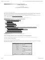
tools, you have to define a system which is mainly composed of several processors and tasks. To define a processor, choose the "Edit/Add/Add a processor" submenu.
The window below is then displayed :
A processor is defined by the following fields :
1 sur 19
21/12/2006 14:16
Cheddar 1.3p2 user's guide
file:///C:/Documents%20and%20Settings/singhoff/Bureau/old/Che...
1. The name of the processor. A processor name can be any combinaison of literal characters including underscore. Space is forbidden. Of course, each processor of
a system should have a unique name.
2. The scheduler hosted by the processor. Basically, you can choose from 6 schedulers (to get a detailed description on these schedulers, see your prefered real time
books) :
Earliest Deadline First (EDF). Tasks can be periodic or not and are scheduled according to their deadline.
Least Laxity First (LLF). Tasks can be periodic or not and are scheduled according to their laxity.
Rate Monotonic. Tasks have to be periodic and deadline must be equal to period. Tasks are scheduled according to their period. You have to be warned that
the value of the priority field of the tasks is ignored here.
Deadline Monotonic. Tasks have to be periodic and are scheduled according to their deadline. You have to be warned that the value of the priority field of
the tasks is ignored here.
POSIX 4 scheduler. Tasks can be periodic or not. Tasks are scheduled according to the priority and the policy of the tasks. (Rate Monotonic and Deadline
Monotonic use the same scheduler engine except that priorities are automaticly computed from task period or deadline). POSIX 4 scheduler supports
SCHED_RR, SCHED_FIFO and SCHED_OTHERS queueing policies. SCHED_OTHERS is a time sharing policy. SCHED_RR and SCHED_FIFO tasks must have priorities
range from 255 to 1. Priority level 0 is reserved to SCHED_OTHERS tasks. The highiest priority level is 255.
user-defined scheduler. This last one allows user to define their own scheduler into Cheddar (see section IV for details).
3. If the scheduler is preemptive or not. By default, the scheduler is set to be preemptive.
4. The quantum value associated to the scheduler. This information is useful if a scheduler have to manage several tasks with the same dynamic or static priority : in
this case, the simulator has to choose how to share the processor between these tasks. The quantum is a bound on the delay a task can hold the processor (if the
quantum is equal to zero, there is no bound on the processor holding time). The quantum value is also used with a POSIX 4 scheduler when some SCHED_RR
tasks are defined. With POSIX.4, two SCHED_RR tasks with the same priority level should share the processor with a round-robin policy. In this case, the
quantum value is the slot time of this round-robin scheduler. Finally, the quantum value could also be used for user-defined scheduler (see part IV for details).
5. The file name : it's the name of a file which contains the source code of a user-defined scheduler (see section IV for details).
Warning : with Cheddar, to add a processor (or an other object), you have to push the Add button before pushing the Close button. That's allow you to quickly define
several objects whithout closing the "Add" window (you should then push Add for each defined object).
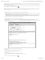
Let's see now how to define a task. Choose the "Edit/Add/Add a task " submenu. The window below is then displayed :
This window is composed of 3 sub-windows : the "main page", the "offset page" and the "user's defined parameters page". The main page contains the following
information :
.
1. At least, a task is defined by a name (the task name should be unique), a capacity (bound on its execution time) and a place to run it (a processor name). The
other parameters are optionnals but can be required for a particular scheduler
2. A type of task . It describes the way the task is activated. An aperiodic task is only activated once time. A periodic task is activated many times and the delay
between two activations is a fixed one. A poisson process task is activated many times and the delay between two activations is a random delay : the random law
used to generated these delays is an exponential one (poisson process). If the task type is "user-defined", the task activation law is defined by the user (see section
IV.2 of this user's guide).
3. The period. It is the time between two task activations. The period is a constant delay for periodic task. It's a average delay for poisson process task. If you
selected a processor that owns a Rate Monotonic or a Deadline Monotonic scheduler, you have to give a period for each of its task
4. A start time. It is the time when the task arrives in the system (its first activation time).
5. A deadline. The task must finish its activation before its deadline. A deadline is a relative information : to get the absolute date at which a task must end an
activation, you should add to the task deadline the time when the task was awoken/activated. Warning : the deadline must be equal to the period if you define a
Rate Monotonic scheduler.
6. A priority and a policy. These parameters are dedicated to the Highiest Priority First/POSIX.4 scheduler. Priority is the fixed priority of a task. Policy can be
SCHED_RR, SCHED_FIFO or SCHED_OTHERS and described how the scheduler choose a task when several tasks have the same priority level. Warning : the priority
and the policy are ignored by a Rate Monotonic and a Deadline Monotonic scheduler.
7. A blocking time. It's a bound on shared resource waiting time. This delay could be set by the user but could also be computed by Cheddar if you described how
shared resources are accessed.
8. An activation rule. The name of the rule which defines the way the task should be activated. Only used with user-defined task. (see section IV for details).
9. A seed . If you defined a poisson process task or a user-defined task you can set here how random activation delay should be generated (in a deterministic way or
not). The "Seed" button proposes you a randomly generated seed value but of course, you can give any seed value. This seed value is used only if the Predictable
button is pushed. If the Unpredictable button is pushed instead, the seed is initialized at simulation time with "gettimeofday".
The second and the third page stored task information which are less used by user's.
2 sur 19
21/12/2006 14:16
Cheddar 1.3p2 user's guide
file:///C:/Documents%20and%20Settings/singhoff/Bureau/old/Che...
The offsets page is made of a table. Each entry of the table stores two information : an activation number and and value. The offset page allows the user to change the
wake up time of a task on a given activation number. For each activation number stored in the "Activations:" fields, the task wake up time will be delayed by the
amount of time given in the "Values" fields.
Finally, the third page (the "User's defined parameters" page) contains task parameters (similar to the deadline, the period, he capacity ...) used by specific scheduler.
The "User's defined parameters page" is described in section IV.4 .
Warning : when you create tasks, in most of cases, Cheddar does not check if your task parameters are erronous according to the scheduler you previously selected :
these checks are done at task analysis/scheduling. Of course, you can always change task and processor parameters with "Edit/Update ", "Edit/Delete" and
"Edit/Duplicate" menus.
When tasks and processors are defined, we can start task analysis. Cheddar provides two kind of analysis tools :
1. Feasibility analysis tools : these tools computes much information without scheduling the set of the tasks. Equation references used to compute theses feasibility
informations are always provided with the results. Feasibility services are provided for tasks and buffers.
2. Simulation analysis tools : With these tools, scheduling have to be computed first. When the scheduling is computing (of course, this step can be long to proceed
...), the resulting scheduling is drawn in the top part of the window and information is computed and displayed in the bottom part of the window. Information
retrived there are only valid in the computed scheduling.The simpliest tools provided by Cheddar checks if a set of tasks meet their temporal constraints.
Simulation services are also provided for other resources (for buffers for instance).
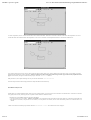
All these tools can be called from the " Tools" Menu and from some toolbar Buttons :
From the submenu "Tools/Scheduling/Scheduling simulation", the scheduling of each processor is drawn on the top of the Cheddar main window (see
below). From the drawn scheduling, missed deadlines are shown and some statistics are displayed (number of preemption for instance).
From the submenu "Tools/Scheduling/Scheduling feasibility", response time, base period and processor utilization level are computed and displayed on the
bottom of the Cheddar main window.
In the bottom part of this window, each resource and task is shown by a time line.
For a time line of a task :
Each vertical red line means that the task is activated (or woken up) at this time.
Each black rectangle means that the task is running at this time.
For a time line of a resource :
Each vertical blue line means that the resource is allocated by a task at this time.
Each black rectangle means that the resource is used by the task which is running at this time.
To get a summary of the tools provided by Cheddar, see section VI .
3 sur 19
21/12/2006 14:16
Cheddar 1.3p2 user's guide
file:///C:/Documents%20and%20Settings/singhoff/Bureau/old/Che...
I.2 Other scheduling analysis tools.
From the "Tools/Scheduling" submenu, you can also access to the following services :
1. The submenu "Tools/Scheduling/Set priorities according to Rate Monotonic" provides a way to change task priorities according to the Rate Monotonic
algorithm : priorities are then modified according to the task periods.
2. The submenu "Tools/Scheduling/Set priorities according to Deadline Monotonic" provides a way to change task priorities according to the Deadline
Monotonic algorithm : priorities are then modified according to the task deadlines.
3. The submenu "Tools/Scheduling/Options" allows you to tune the way scheduling simulations are done : see section I.3 .
I.3 Scheduling options.
The submenu "Tools/Scheduling/Options" allows you to tune the way scheduling simulations are done (see the window above) :
If you push the "Resource" button, access to shared ressources will be done during simulation. By default, all shared resources are ignored.
If you push the "Offsets" button, the simulation engine takes care of the task offsets given at task definition time : task activations can be then delayed if you
provided offset values at task definition time.
If you push the "Precedencies" button, task scheduling will be done so that task precedencies will be meet. By default, task precedencies are ignored.
Finally, Cheddar allows you to randomly activated tasks. If you want to do simulations with this kind of task, the simulator engive have to compute some random
values. From this window, you can tune the way random activation delays are generated. A seed value can be associated for each task but you also can use only
one seed for all tasks. In the two cases, you can do "predictable" or "unpredictable" simulations. If you choose "predictable" simulation, the seed will be initialized
by a given value. In the other case, the seed is initialized with "gettimeofday". . Pushing the "Predictable for all tasks" radio button leads to take the seed
value of the Option window during simulation for all tasks. If the "Task specific seed" radio button is pushed instead, the seed of each task is used to generate
task activation delays. You should notice that by default, 0 is given to the seed value, but of course, you can choose any value. Pushing the "Seed" button give you
a random value for the seed.
II. About Cheddar project files.
Information stored during a simulation can be saved into project files. A project file is a XML file defined by this DTD. By the way, you do not need a deep
understanding of the layout of cheddar project files except if you want to edit project files by hand. If so, you should check if your project files are correctly structured
by the tool dump_sys (dump_sys just read, parses and displays to the screen the content of a XML Cheddar project file).
All Cheddar XML files can be displayed with an Internet Browser if you put in the directory hosting your XML Cheddar files the following XSLT file and the
following.CSS file. To do so, you should use a recent release of Internet Explorer (version 6.0 or later), Netscape (version 7.0 or later) or Mozilla (version 1.0 or later).
From Cheddar, there is two ways to load a project file :
Firstly, a project file can be loaded from the "File/Open" submenu. Just click on the Open button, and give the file name of your project.
Secondly, a project can be loaded from the command line. For instance, to start Cheddar and load the project file my_project.xml, just do :
my_shell$cheddar my_project.xml
Saving a project can be done with the same "File" menu.
III. Scheduling with task dependencies
This chapter describes services provided by Cheddar when the system you want to study has task dependencies. By task dependencies, we mean resources shared by
several tasks (ex : semaphores) or precedencies relationship between several tasks (due to buffer access or message exchange or also constraints between the end of a
task and the start of another one).
III.1 Shared resources analysis tools.
4 sur 19
21/12/2006 14:16
Cheddar 1.3p2 user's guide
file:///C:/Documents%20and%20Settings/singhoff/Bureau/old/Che...
With Cheddar, you can define shared resources. Shared resources can be seen as semaphores. They can be accessed by several tasks. Tasks which require access to an
already allocated semaphore are blocked (and then, unscheduled). To define a shared resource in a Cheddar project, call the submenu "Edit/Add/Add a resource".
The window below is then displayed :
Before adding a shared resource, at least one processor and one task must already exist in your project. A resource is defined by :
1. An unique name.
2. An initial value (simular to a semaphore initial value). During a scheduling simulation, at a given time, if a resource value is equal to zero, requiring tasks are
blocked up to the semaphore is released.
3. A protocol. Today, you can choose between PCP, PIP or "No protocol". With PCP or PIP, access to shared resources may change task priorities (See a
real time book to have details). The last protocol just means that no task prioriy will be changed at shared resource access.
must have an unique name and an initial value. For each resource, you should select a protocol which manages the way the resources are allocated/released. Today, 3
protocols are available : PCP, PIP or no protocol. During resource allocation, no protocol does not change task priorities and only checks if the resource is free or not.
See a real time book to have details on PCP and PIP.
Of course, you have to select a processor where the resource will be attach. Finally, we must give information on tasks who need the resource. Tasks held resources in
critical section. So, you have to give, the start and the end of each critical section.
By default, shared resources analysis tools are not included in the scheduling simulation engine of Cheddar. See "Tools/Scheduling/Options" if you want to take care
of shared resources during scheduling simulation.
In the "Tools/Resources/Blocking time", you will find services to compute bounds on blocking time of each tasks.
III.2 Task precedencies analysis tools.
With Cheddar, dependencies are links between at least two tasks. There are three different types of dependencies : precedencies, message and buffer dependencies.
Precendencies express order constraints between end or begin of task execution. Message dependencies expressed relationship between a sender and a receiver task of a
given message. Buffer dependencies expressed relationship between producer and consumer of data in a given buffer.
To create a dependency, you may open the "Precedencies Graph" window by clicking on the appropriate icon on the main Cheddar window. By the way, all Cheddar
objects are imported in this window. All items are represented by geometrical forms :
Tasks -> circles.
Messages -> rectangles.
Buffers -> enveloppes.
If there is no item on the canvas, it means that you don't have created any dependency before... So you can create one by entering in "create" mode (on the top left
corner) and selecting 'task' on the radio button. After that, create a task by clicking on the canvas, then a popup appears asking you to create a new or import one task
from Cheddar (cf Part One). It's the same succession of operations to create others types of items (buffers and messages).
5 sur 19
21/12/2006 14:16
Cheddar 1.3p2 user's guide
file:///C:/Documents%20and%20Settings/singhoff/Bureau/old/Che...
To create a dependencie, enter in "create" mode and select 'arrow' on the radio button. Then click on a first item. This item is the source of the dependencie. Click on a
second item which will be the destination of the dependencie. You can see a screenshot of such a dependencie between a task and and a buffer below :
If you want to delete nodes or arrows, enter in "delete" mode and select the object (task, arrow, message, buffer) on the radio button. Click on a task, buffer or message
should delete all dependencies of the clicked object. Delete operations do not delete tasks, buffers and messages from the project files but only dependencies of the
project. To delete tasks, messages or buffers from the project, choose the "Edit/Delete" submenu.
With precedencies, some simple scheduling tools are provided. See the submenu "Tools/Precedencies"
End to end response time includes message transmission delay and buffer memorisation delay.
III.3 Buffer analysis tools.
Cheddar allows you to define buffers shared by tasks. If you want to define a buffer, a processor and a least one task have to be defined before. At the time we writte this
user's guide, buffers can only shared by periodics or aperiodicss tasks. Buffers are defined as follow :
A buffer has a unique name, a size and is hosted by a processor.
Two type of tasks can access a buffer : producer and consumer . We suppose that a producer/consumer writes/reads a fixed size of information in the buffer each
time the task is activated (in the periodic case for instance). For each producer or consumer, the size of the information produced or consummed have to be
defined.
A buffer can be added to a Cheddar project with the submenu "Edit/Add/Add a buffer". The window below is then displayed :
6 sur 19
21/12/2006 14:16
Cheddar 1.3p2 user's guide
file:///C:/Documents%20and%20Settings/singhoff/Bureau/old/Che...
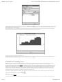
Like tasks, from a buffer, two kind of tools can be invoke by the user : simulation and feasibility tools. At first, simulation of the task scheduling can help the user to
see how the buffer is filled or not with messages (see "Tools/Buffer/Buffer simulation" submenu). In this case, a scheduling simulation must be previously run. The
result is then displayed in a window as below :
Buffer Feasibility mainly consits to compute buffer bounds. Bounds computed here suppose that each task which is defined as "procuder", produces one message per
periodic activation. In the same manner, each "consumer" extracts one message during each of its periodic activation.
The picture contains for each time the buffer utilization level.
Secondly, the feasibility tool provides a way to compute bound on buffer utilization level. At the time we write this User's guide, bounds do not depend on the type of
the scheduler. Bounds can be computed from the "Tools/Buffer/Buffer feasibility" submenu.
IV. Multiprocessor scheduling services.
Multiprocessor system is good for heavy computing demands. It is sometimes only way to provide sufficient processing power to meet critical real-time deadlines.
Multiprocessor systems are also in generally more reliable than uni-processor systems. Scheduling of multiprocessor systems is proven to be NP-hard
(Non-deterministic Polynomial-time) problem [LEU 82]. The complexity class NP is the set of decision problems that can be solved by a non-deterministic machine in
polynomial time. Complexity theory is part of the theory of computation dealing with the resources required during computation to solve a given problem. The most
common resources are time (how many steps does it take to solve a problem) and space (how much memory does it take to solve a problem). Other resources can also
be considered, such as how many parallel processors are needed to solve a problem in parallel. There are many scheduling heuristics to solve this. Rate-monotonic
scheduling is good for numerous reasons: Rate-monotonic algorithm is optimal for fixed priority assignment of periodic tasks on a processor so it’s easy to design
predictable real-time system. Also it’s easy to implement and takes minimal scheduling overhead.
Cheddar has four algorithms: RMNF, RMFF, RMBF, RMST and RMGT. Each of these are off-line schemes, so entire task set must be known before starting task
assignment. Bounds for functions are calculated using
.
Rate-Monotonic-Next-Fit [SON 93]
Upper bound for this algorithm is 2.67. Tasks are sorted non-decreasing order of periods. Then tasks are placed on processors, according to Condition IP(Increasing
7 sur 19
21/12/2006 14:16
Cheddar 1.3p2 user's guide
file:///C:/Documents%20and%20Settings/singhoff/Bureau/old/Che...
Period). First task is placed on first processor. Then second task is placed on first processor, if it meets Condition IP. Otherwise it is placed on new processor. This
continues until all tasks are scheduled.
Rate-Monotonic-First-Fit [SON 93]
Upper bound for this algorithm is 2.33 [SON 93] (original study by Liu and Dhall had wrong bound of 2.23). Tasks are sorted non-decreasing order of periods.
Condition IP is used to verify schedulability of tasks on processors. First task is placed on first processor. Then second task is placed on first processor, if it meets
Condition IP. Otherwise it is placed on new processor. Third task is tried to place on first processor according to Condition IP. If it does not meet condition, task is tried
to place on second processor. Otherwise new processor is selected for third task…
Rate-Monotonic-Best-Fit [SON 93]
Upper bound for this algorithm is 2.33. Tasks are sorted non-decreasing order of periods. First task is placed on first processor. For second task, function checks all
processors, if it meets Condition IP. For processors which satisfy condition, it checks where kj is number of tasks already assigned to processor and Uj total utilization
of the kj tasks. And task is assigned to processor which has smallest value. If condition is not met, new processor is selected for task.
Rate-Monotonic Small-Tasks [BUR 94]
Upper bound for RMST is
, a = max Ui, i = 1,…,K and U is utilization of all tasks. Tasks are sorted increasing Si. Si = log2(Ti). Main idea of RMST is to
minimize value of b for each processor. ß = max Si – min Si, 1= i =K.
Rate-Monotonic General-Tasks [BUR 94]
Upper bound for RMGT is 1.75. RMGT uses RMST algorithm for task s = 1/3 and First-Fit heuristics for rest of tasks.
Example of use :
1. First, Define processors for tasks. They have to be Rate Monotonic type.
2. Second, Define tasks (host tasks on any processors)
8 sur 19
21/12/2006 14:16
Cheddar 1.3p2 user's guide
file:///C:/Documents%20and%20Settings/singhoff/Bureau/old/Che...
3. Third, compute partitioning :
IV. User-defined task arrival patterns and schedulers : how to easily define new schedulers and task
arrival patterns.
Feasibillity tests are limited to only few task models (mainly periodic tasks) and to only few schedulers. When you have to test feasibility of an application built with a
particular task model and scheduled with a particular scheduler, you can not used any more feasibility tests implemented into cheddar. To test if such application meet
its temporal constraint the only solution is to do scheduling simulation and to do analysing of the computed scheduling. This section describes a functionnality provided
by Cheddar which allows you to design and easily code your own schedulers and tasks models so that you can use the simulation features of Cheddar to check is task
deadlines are meet.
9 sur 19
21/12/2006 14:16
Cheddar 1.3p2 user's guide
file:///C:/Documents%20and%20Settings/singhoff/Bureau/old/Che...
The picture above give a you a short idea about the way schedulers are implemented into Cheddar. Basically, all tasks are stored in a simple table called the "TCB
table" (this table is indexed from 0 to the number of tasks in the system). The job of a scheduler is to find a task to run from a set of ready tasks. To achieve this job,
Cheddar models a scheduler with a 3 stages pipe-line which is similar to the POSIX.4 scheduler. These 3 stages are :
1. The priority stage : for each ready task, a dynamic priority is computed.
2. The queueing stage : ready tasks are inserted into different queues. It exists one queue per dynamic priority level. Each queue contains all the ready tasks with
the same dynamic priority value.
3. The election stage : the scheduler looks for the non empty queue with the highiest priority level and give the processor to the task in the head of this queue. The
elected task keeps the processor durring one unit of time if the design scheduler is preemptive or during all its capacity if the scheduler is non preemptive.
Defining a new scheduler is simply giving piece of code for some of the pipe-line stages we described above. Each of these stages can be defined by a user without the
need to have a deep kwonledge of the way the scheduling simulator works.
schedulers defined by a user are stored in text files. These files are organized in several sections :
The start section. In this section, you may defined variables needed to schedule your tasks. Many variables are already predefined in Cheddar. Two varaible
families exist : static and dynamic variables. Static variables are those defined at task definition (ex : period, deadline, capacity ...). Values of static variables
never change during simulation and are given when the user describes the system he want to study (ex : with the "Edit/Add/Add a Task" submenu). Dynamic
variables are data collected by the simulator. They show the state of task, processor and the other objets of system during the simulation time. Then, dynamic
variables can change during simulation. See section IV.4 for a list of all predefined static and dynamic variables. Static and dynamic variables declared in the
start section can be of 6 different types : scalar type (double, integer or boolean) and table type (integer_task_array, boolean_task_array or
double_task_array). A table type is a variable which store one data for each task. As we said previously, all the tasks of the system are stored in a simple table
(the TCB table). Users do not directly manipulate this table but can access to it througth table type variables.
The priority section. The code given here is called each time a scheduling decision have to be token (at each unit of time for preemptive scheduler and when a
task run during all his capacity for non preemptive scheduler). The code given here can be composed of many differents statements described in section IV.4
The election section. This section just decides which task should receive the processor for next units of time. Today, this section can only be made of one return
statement.
The task activation section. This part describes how tasks could be activated during a simulation. In Cheddar, 3 kinds of tasks exists : aperiodic tasks which are
activated only one time and periodic or poissons process tasks which are activated several times. In the case of periodic tasks, two successive task activations are
delayed by an amount of fixed time called period. In the case of poisson process tasks, two successive task activations are delayed by a exponential random delay.
The task activation section allows you to define new kinds of task activation laws.
In the sequel, we first give you some simple examples of user-defined scheduler. Then, we explain how to use this kind of scheduler to do scheduling simulation with
Cheddar.The list of statements and the list of predefined variables is given at the end of this section. Finally, this section is ended with an explanation of the most
common errors.
V.1 Examples of user-defined schedulers.
In this section, we give some user-defined scheduler examples. We first show that user-defined scheduler can be built with two kinds of statements : high-level and
low-level statements. Secondly, we present how to add new task parameters with User's defined task parameters.
IV.1.1 Low-level statements versus High-level statements
Let see now some very simple user-defined schedulers. The most simple user-defined scheduler can be defined like below :
election_section:
return min_to_index(period);
Figure 1. a simple Rate Monotonic scheduler
This first example shows you how to give the processor to the task with the smallest period. This scheduler is equivalent to the Rate monotonic implemented into
Cheddar. period is a predefined static variable initialized at task definition time by the user. To implement a Rate Monotonic scheduler, no dynamic priorities are
computed and no variable is necessary. Then, the scheduler designer does not have to redefine the start and priority sections. The only section which is defined is the
election one. The election section contains an unique return statement to inform the scheduling simulator engine which task should be run for the next unit of time.
The return statement uses the high level min_to_index operator. This operator scans the TCB table to find the ready task with the minimum value for the static variable
10 sur 19
21/12/2006 14:16
Cheddar 1.3p2 user's guide
file:///C:/Documents%20and%20Settings/singhoff/Bureau/old/Che...
period. In Cheddar, the scheduler designer can use two kinds of statements : high-level and low-level statements. High level statements like min_to_index, hides the
data type organization of the scheduling simulator engine. For example, the scheduler designer do not need to give statement into its user-defined scheduler to scan
manually the TCB table. Writting scheduler with high-level statements is then an easy work. At contrary, low-level statements assume that the user have a deeper idea
of the design of the scheduling engine simulator. By the way, these statements are sometimes necessary when the scheduler designer want code a too much specific
scheduler.
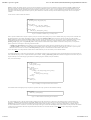
Let see now how to define an EDF like scheduler :
1 start_section:
2
dynamic_priority : integer_task_array;
3
4
5 priority_section:
6
dynamic_priority := start_time + deadline
7
+ ((activation_number-1)*period);
8
9 election_section:
10
return min_to_index(dynamic_priority);
Figure 2. an EDF like scheduler using vectorial operators
EDF is a dynamic scheduler which computes a dynamic priority for each task. This dynamic priority is in fact a deadline. EDF just gives the processor to the task with
the shortest deadline. In our example, this deadline is stored in a variable called dynamic_deadline. Since we need one value per task, the type of this variable is
integer_task_array. With this example the priority_section is not empty any more and contains (lines 5 to 7) the necessary code to compute EDF dynamic priorities.
You should notice that the code in line 6/7 is in fact a vectorial operation : the arithmetic operation to compute the deadline is done for each item of the table
dynamic_priority ranging from 1 to nb_tasks (nb_tasks is a static predefined variable initialized by the number of tasks in the current processor). To compute the
dynamic priorities of our example, we used many predefined variables :
deadline, start_time and period : it's the deadline, start time and period values given by the user at task definition time (in the window Edit/Add/add a task).
activation_number : it's a dynamic variable updated by the simulation engine. The simulator increments this variable each time a periodic or a poisson process
task start a new activation. For instance, if activation_number[i] is equal to 3, it means that the task i has started its 4th activation.
You can find in IV.4 a list of all predefined variables and all available statements you can used to build your user-defined scheduler.
The exampleof the figure 2. is built with vectorial operators : each arithmetic operation is done for all tak of the system. The scheduler designer do not need to take care
of the TCB table and just give rules to computed the EDF dynamic deadline. As max_to_index/min_to_index, these statements are High-level ones because they do not
required to directly access to the data type organization of the scheduling engine of Cheddar (mainly the TCB table).
Now, let see a third example:
start_section:
to_run : integer;
current_priority : integer;
priority_section:
current_priority:=0;
forall i loop
if (ready[i] = true) and (priority[i]>current_priority)
then to_run:=i;
current_priority:=priority[i];
end if;
end loop;
election_section:
return to_run;
Figure 3. Building a user-defined with low-level statement
This scheduler looks for the highest priority ready task of a processor and is fully equivalent to the scheduler described by :
election_section:
return max_to_index(priority);
Figure 4. a HPF scheduler built with hight-level statements
but, in the example of Figure 3, the code scans itself the TCB table to find a ready task to be run. To achieve this, the example of Figure 3 is built with low-level
instructions : a forall loop and an if statement. The priority_section is then composed of a loop which do a test on each TCB table entry. This loop is made with a
forall statement, a loop which run the enclosed statement for each task defined in the TCB table. To contrary to a high-level implementation, a scheduler made of
low-level statements have to do more tests. For instance, the example of the Figure 3 checks with the ready dynamic variable if tasks are ready at the time the scheduler
is called. Low-level scheduler are then more complicated and more difficult to test. The reader will find in section IV.3 some tips to help testing of complicated
user-defined scheduler.
11 sur 19
21/12/2006 14:16
Cheddar 1.3p2 user's guide
file:///C:/Documents%20and%20Settings/singhoff/Bureau/old/Che...
V.1.2 user-defined scheduler built with User's defined Task Parameters
In the previous examples, data used to built user-defined scheduler was either static variable initialized at task definition time, either dynamic variables predefined or
declared in the start section. A last type of data exists in Cheddar : User's defined task parameters. This kinds of data are static ones and are defined at task definition
time. User's defined task parameters allow the user to extend the set of static variables. Since they describe new task parameters, User's defined task parameters are table
type. Today, User's defined task parameters can be boolean, integer, double or string table type. To define User's defined task parameters, you have to update the second
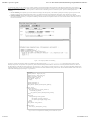
page of the book displayed from the submenus "Edit/Add/Add a task" or "Edit/Update/Update a task" :
Figure 5. Adding an Users's Defined Task Parameter
The example above shows you a system composed of 3 tasks (T1, T2 and T3) where a criticity level is defined. Like usual task parameters, you should give a value to an
User's defined task parameter (ex : the criticity level for task T1 is 1) but you also have to set a type to the parameter (integer in our example). When tasks are created,
as usually, you can call the scheduling simulation services of Cheddar. The next window is a snapshoot of the resulting scheduling of our example composed of 3 tasks
scheduled according to their criticity level. (T2 is the most critical task and T1 the less critical).
Figure 6. Scheduling according to a criticity level.
12 sur 19
21/12/2006 14:16
Cheddar 1.3p2 user's guide
file:///C:/Documents%20and%20Settings/singhoff/Bureau/old/Che...
To conclude this chapter, let see a look on a more complex example of user-defined scheduler which summarises all the features presented before. This example is an
ARINC 653 scheduler (see [ARI 97]). An ARINC 653 system is composed of several partitions. A partition is an unit of software and is itself composed of processes
and memory spaces. A processor can hosts several partitions so that two levels of scheduling exists in an ARINC653 system : partition scheduling and process
scheduling.
1. Process scheduling. In one partition, process are scheduled according to their fixed priority. The scheduler is preemptive and always gives the processor to the
highiest fixed priority task of the partition which is ready to run. When several tasks of a partition has the same priority level, the oldest one is elected.
2. Partition scheduling. Partitions share the processor in a predefined way. On each processor partitions are activated according to an activation table. This table is
built at design time and defines a cycle of partition scheduling. The table describes for each partition when it has to be activated and how much time it has to run
for each of its activation.
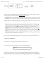
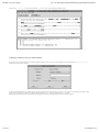
Figure 7. An example of ARINC 653 scheduling
The Figure 7. displays an example of ARINC 653 scheduling (see the XML project file project_examples/arinc653.xml). The studied system is made of 3 tasks
hosted by one processor. The processor owns 2 partitions : partition number P0 and partition number P1. The task T1 run into the partition P0 and the two others run
into the partition P1. Each task has a fixed priority level : the T1 priority is 1, the T2 priority is 5 and the T3 priority is 4. The cyclic partition scheduling should be done
so that P0 run before P1. In each cycle, P0 should be run during 2 units of time and P1 should run during 4 units of time. The user-defined scheduler source code used to
compute the scheduling displayed in Figure 7 is given bellow :
start_section:
partition_duration : integer_task_array;
dynamic_priority : integer_task_array;
number_of_partition : integer :=2;
current_partition : integer :=0;
time_partition : integer :=0;
i : integer;
partition_duration[0]:=2;
partition_duration[1]:=4;
time_partition:=partition_duration[current_partition];
priority_section:
if time_partition=0
then current_partition:=(current_partition+1)
mod number_of_partition;
time_partition:=partition_duration[current_partition];
end if;
forall i loop
if task_partition[i]=current_partition
then dynamic_priority[i]:=priority[i];
else dynamic_priority[i]0; ready[i]:=false;
end if;
end loop;
time_partition:=time_partition-1;
election_section:
return max_to_index(dynamic_priority);
Figure 8. Processes and partitions scheduling into an ARINC 653 system
13 sur 19
21/12/2006 14:16
Cheddar 1.3p2 user's guide
file:///C:/Documents%20and%20Settings/singhoff/Bureau/old/Che...
In this code, task_partition is an User's defined task parameter. task_partition stores the partition number hosting the associated task. The variable partition_duration
stores the partition cyclic activation table.
V.2 Scheduling with specific task models.
In the same way you can define specific schedulers, you can also define specific task activation laws. By default, 3 kinds of task activation law are defined in Cheddar :
Periodic task : a fixed amount of time exists between two successive task activations.
Aperiodic task : the task is activated only one time at a given time.
Poisson process task : tasks are activated several times and the delay between two successive activations is a random delay. The static variable period in this case
is the average time between two successive activations. Delay between activations are generetad according to a random poisson process.
If the application you want to study can not be modeled with this 3 kinds of activation rules above, a possible solution is to explain your own task activation law with a
user-defined scheduler. The description of task activation law is done in .sc files in a particulary section which is called task_activation_section. In this section, you
can define named activation rules with set statements. The set statement just link a name/identifier (the left part ot the set statement) and an expression (the right part of
the set statement). The expression explained the amount of time the scheduling simulator engine have to wait between two activation of a given task.
election_section:
return max_to_index(priority);
task_activation_section:
set activation_rule1 10;
set activation_rule2 2*capacity;
set activation_rule3 exponential;
set activation_rule4 uniform;
Figure 8. Defining new task activation laws : how to run simulation with specific task models
The example of the figure 8 describes a Highiest Priority First scheduler which hosts tasks activated with different laws. Each law is described by a set statement :
The law activation_rule1 describes that some tasks are periodics (with a period equal to 10).
The law activation_rule2 describes that some tasks are periodics (with a period equal to twice their capacity).
The law activation_rule3 describes randomly activated tasks. Two successive activations are delayed by a amount of time which is randomly computed. Delays
are computed according to a random exponential distribution law with a mean value of period. The seed used during random delay generation depend of the
scheduling options set at simulation time (see section I.3 ) : the user can choose to associate a seed per task or a seed for all the tasks. Seeds can be initialized in a
predictable way or in an unpredictable way. In the case of a predictable seed, the random generator is initialized with the seed value given at task definition time
or in the scheduling option window. In the case of a unpredictable seed, the seed is initialized by the "gettimeofday" at simulation time.
The law activation_rule4 describes randomly activated tasks. Two successive activations are delayed by a amount of time which is randomly computed. Delays
are computed according to a random uniform distribution law with a mean value of period. The seed used during random delay generation is managed in the
same way that activation_rule3.
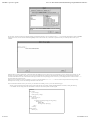
When task activation rules are defined, task activation names (ex : activation_rule1) have to be associated to "real" task. The picture bellow shows you an
"Edit/Add/Add a task" window :
In this example (see the XML project file project_examples/test_user-defined6.xml), the task activation rule activation_rule1 is associated to the task T1. The
task activation rule activation_rule2 is associated to the task T2. The task activation rule activation_rule3 is associated to the tasks T3, T4 and T5. Finally, the task
14 sur 19
21/12/2006 14:16
Cheddar 1.3p2 user's guide
file:///C:/Documents%20and%20Settings/singhoff/Bureau/old/Che...
activation rule activation_rule4 is associated to the tasks T6, T7 and T8. Then, a possible resulting scheduling can be :
V.3 Running a simulation with a user-defined scheduler.
Let see how to run a simulation with one or several user-defined schedulers. Firstly, you have to add a scheduler by selecting the submenu "Edit/Add a processor".
The following window is then launched :
To add a user-defined scheduler into a Cheddar project, select the right item of the Combo Box and give a name to your scheduler. You should then provide the code of
your user-defined scheduler. This operation can be done either by pushing the "Edit" button or by pushing the "Read" button.
In the first case, the following window is spawned and you should give a file name containing the code of your user-defined scheduler :
15 sur 19
21/12/2006 14:16
Cheddar 1.3p2 user's guide
file:///C:/Documents%20and%20Settings/singhoff/Bureau/old/Che...
By convention, files which contain user-defined scheduler code should be prefixed by .sc. For example, the file rm.sc in our example should almost contains an election
section and of course, can also contains a start and a priority sections. In the second case, a small editor is spawned so that you can directly edit the code of your
scheduler :
When the editor is closed (by pushing the Ok button) and when the Cheddar project is saved, the code of your scheduler is saved in a text file also prefixed by .sc. The
file name is choosen by Cheddar if you did not give one at processor definition time. Note that in the resulting XML Cheddar project file, the file name storing the
user-defined scheduler source code is referenced in a XML tag associated to the corresponding processor. Of course, you can change the name of this file and one ".sc"
file can be shared by several processors.
When a processor is defined, you have to add tasks on it. To do so, select the submenu "Edit/Add a task" like in section I. Just place the task on the previously
defined processor. Finally, you can run scheduling simulations as the usual case.
Since a user-defined scheduler is also a piece of code, you sometimes need to debug it. To do, you can use the following tips :
Firstly, a special instruction can be used to display at the screen the value of a dynamic variable : the put statement. For instance, running the following
user-defined code will display each time the scheduler is called, the value of the dynamic variable to_run :
--!TRACE
start_section:
to_run : integer;
current_priority : integer;
priority_section:
current_priority:=0;
forall i loop
if (ready[i]=true) and (priority[i]>current_priority)
then to_run:=i;
put(to_run);
current_priority:=priority[i];
end if;
end loop;
election_section:
return to_run;
16 sur 19
21/12/2006 14:16
Cheddar 1.3p2 user's guide
file:///C:/Documents%20and%20Settings/singhoff/Bureau/old/Che...
A second tip can help you to test if the syntax of your user-defined scheduler is correct. In all .sc file, you can add else where the line --!TRACE. If you add this
line, the parser will give extra information during the syntax analisys of your user-defined scheduler. It's usefull if you want to test a .sc file before using it in a
Cheddar project file. You can also test it with sc, a program designed to read, parse and check .sc files.
Finally, to quickly change and test your user-defined scheduler, you can launched a small editor from the submenu Edit/Edit a scheduler (see the window
above). This editor stays open until you pressed the Close button. Even if this window still open, you can call all the other services provided by Cheddar
(including scheduling simulation services). After you had changed the code of your user-defined scheduler, pushing the Modify button provides your modified
code to the simulation engine. Then, you can quickly change your user-defined code without closing the editor between two simulations.
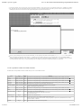
V.4 List of predefined variables and available statements.
The table bellow list all predefined variables available when you write a user-defined scheduler :
Type
Family
period
Name
integer_task_array
static
Store the value of the parameter given at task definition time. For the meaning of this variable, see section I.
Meaning
deadline
integer_task_array
static
Store the value of the parameter given at task definition time. For the meaning of this variable, see section I.
capacity
integer_task_array
static
Store the value of the parameter given at task definition time. For the meaning of this variable, see section I.
start_time
integer_task_array
static
Store the value of the parameter given at task definition time. For the meaning of this variable, see section I.
used_cpu
integer_task_array dynamic Store the amount of processor time wasted by the associated task.
activation_number integer_task_array dynamic Store the activation number of the associated task. Of course, using this
variable is meaningless for aperiodic tasks.
jitter
integer_task_array
static
Store the value of the parameter given at task definition time. For the meaning of this variable, see section I.
priority
integer_task_array
static
Store the value of the parameter given at task definition time. For the meaning of this variable, see section I.
previously_elected
simulation_time
rest_of_capacity
nb_tasks
17 sur 19
integer
dynamic At the time the user-defined scheduler run,
this variable store the TCB index of the task elected at the
previous simulation time
integer
dynamic Store the current simulation time .
integer_task_array dynamic For each task activation, this variable is reseted to the capacity each
time the associated task starts a new activation. If rest_of_capacity is equal to zero, the task had over its current
activation and then, is blocked.
integer
static
Given the number of tasks of the current processor.
21/12/2006 14:16
Cheddar 1.3p2 user's guide
ready
file:///C:/Documents%20and%20Settings/singhoff/Bureau/old/Che...
boolean
dynamic Store the state of the task : this boolean is true if the task is ready ; it means the task has a capacity to run, does not
wait for a shared resource, does not wait for a delay, does not wait for a offset constraint and does not wait for a
precedency constraint.
The BNF syntax of a .sc file is given bellow :
entry := start_rule priority_rule election_rule task_activation_rule
declare_rule := "start_section:" statements
priority_rule := "priority_section:" statements
election_rule := "election_section:" statements
task_activation_rule := "task_activation_section" statements
statements := statement {statement}
statement :=
"put" "(" expression ")" ";"
| identifier ':' data_type [ ":=" expression ] ';'
| "if" expression "then" statements [ "else" statements ] "end" "if" ";"
| "return" expr ";"
| "forall" expression "loop" statements "end" "loop" ";"
| "while" expression "loop" statements "end" "loop" ";"
| "set" identifier expression ';'
date_type := "double" | "integer" | "boolean" | "string"
| "integer_task_array" | "double_task_array" | "boolean_task_array" | "string_task_array"
operator := "and" | "or" | "mod" | "<" | ">" | "<=" | ">=" | "/=" | "=" | "+" | "/" | "-" | "*" | "**"
expression := expression operator expression
| "(" expression ")"
| "not" expression
| "-" expression
| "max_to_index" "(" expression ")"
| "min_to_index" "(" expression ")"
| "max" "(" expression "," expression ")"
| "min" "(" expression "," expression ")"
| "lcm " "(" expression "," expression ")"
| "uniform"
| "exponential"
| identifier "[" expression "]"
| identifier
| integer_value
| double_value
| boolean_value
Notes on the BNF of .sc file syntax :
entry is the entry point of the grammar.
The data_type rule describes all data types available in a .sc file
The operator rule lists all binary operators.
The expression rule give all possibles expressions that you can use to define your scheduler.
The statement rule contains all statements which can be used in a .sc file.
identifier is a string constant.
integer_value is a integer constant.
double_value is a double constant.
boolean_value is a boolean constant.
Two kinds of statements exist to build your user-defined scheduler : low-level and high-level statements. high-level statementsoperate on all task informations.
low-level statements operate only on one information of a task at a time. all these statements work as follow :
1. The if statement : works like in C, Ada or most of programming language : run the else or the then statement branch according to the value of the if expression.
2. The while statement : works like in C, Ada or most of programming language : run the statements inclosed in the loop/end loop block until the while condition
become false.
3. The forall statement : it's a loop with a predefined iterator index. With a forall statement, the statements enclosed in the loop is run for each task defined in the
TCB table. At each iteration/task, the variable defined in the forall statement is incremented. Then, its value range from 1 to nb_tasks (nb_tasks is a predefined
static variable initiliazed to the number of tasks hosted by the processor).
4. The return statement. You can use a return statement in two cases :
1. With any argument in any section except in the election_section. In this case, the return statement just end the code of the section.
2. With a integer argument and only in the election_section . Then, the return statement give the task number to be run.
5. The put(p) statement : display to the screen the value of the variable p. It's useful to debug your user-defined scheduler.
6. The set statement : description of new task activation model..
The predefined operators work as follow :
1. lcm(a,b) : return the last common multiplier of a and b.
2. max(a,b) : return the maximum value between a and b.
18 sur 19
21/12/2006 14:16
Cheddar 1.3p2 user's guide
file:///C:/Documents%20and%20Settings/singhoff/Bureau/old/Che...
3. min(a,b) : return the minimum value between a and b.
4. max_to_index (v) : firstly find the task in the TCB with the maximum value of v and then, return its position in the TCB table. Only ready tasks are considered by
this operator.
5. min_to_index(v) : firstly find the task in the TCB with the minimum value of v and then, return its position in the TCB table Only ready tasks are considered by
this operator.
6. a mod b : compute the modulo of a on b (rest of the integer division).
VI. Overview of analysis tools available from the Tools menu.
All Cheddar analysis tools are called from the "Tools" menu. This section gives a short description of them. Some of them compute
tasks parameters, and then are composed of two submenus : "Compute and update tasks set"
and "Compute and display".
Choose "Compute and update tasks set" submenu if you want to save computed parameters into your project tasks set.
Choose "Compute and display" if you only want to display computed parameters on the bottom of the main Cheddar window.
Provided tools are :
1. Clear work space : clean the working area (main window). Do not change anything on the project itself.
2. Scheduling tools : from this submenu, you can do and draw scheduling simulation ("Tools/Scheduling/Scheduling simulation"), compute feasibility tests
such as response time, base period, processor utilization, ... ("Tools/Scheduling/Scheduling feasibility "), set task priorities according to classic scheduling
algorithms (Rate Monotonic and Deadline Monotonic) or tune how scheduling simulation will be done ("Tools/Scheduling/Options").
3. Shared resources tools : from there, you can compute bound on shared resources blocking time. Blocking time evaluation is available for PCP and PIP protocols.
4. Buffers analysis : this submenu can help you to study buffers shared by periodic tasks. At first, you can do simulation of buffer utilization factor from a given
scheduling simulation ("Tools/Buffer/Buffer simulation"). You can also compute bounds on buffers ("Tools/Buffer/Buffer Feasibility").
5. Precedency tools . You will find here some heuristics/algorithms that can schedule or check feasibility of a tasks set with dependencies : task deadlines or task
priorities can be set according to the Chetto and Blazewicz heuristic ("Tools/Precendencies/Chetto/Blazewicz modifications on priorities" and
"Tools/Precendencies/Chetto/Blazewicz modifications on deadlines"), or end to end response time bounds can also be computed with the Holistic
method ("Tools/Precedencies/End to end response time").
6. Random : this submenu should provide necessary tools to do simulations with random events. Today, the only feature provided here is a response time analysis
feature : you can get a statistic distribution of task response time from a scheduling simulation ("Tools/Random/Compute response time density").
Contact : Frank Singhoff mailto:[email protected]
Last update : august the 15th, 2004
19 sur 19
21/12/2006 14:16