Download TGrid 5.0 User's Guide

TGrid 5.0 User’s Guide
April 2008
c 2008 by ANSYS, Inc.
Copyright All Rights Reserved. No part of this document may be reproduced or otherwise used in
any form without express written permission from ANSYS, Inc.
Airpak, ANSYS, ANSYS Workbench, AUTODYN, CFX, FIDAP, FloWizard, FLUENT,
GAMBIT, Icechip, Icemax, Icepak, Icepro, Icewave, MixSim, POLYFLOW, TGrid, and any
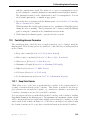
and all ANSYS, Inc. brand, product, service and feature names, logos and slogans are
registered trademarks or trademarks of ANSYS, Inc. or its subsidiaries located in the
United States or other countries. All other brand, product, service and feature names
or trademarks are the property of their respective owners.
CATIA V5 is a registered trademark of Dassault Syst`emes. CHEMKIN is a registered
trademark of Reaction Design Inc.
Portions of this program include material copyrighted by PathScale Corporation
2003-2004.
ANSYS, Inc.
Centerra Resource Park
10 Cavendish Court
Lebanon, NH 03766
Contents
Preface
UTM-1
1 Introduction to TGrid
1-1
1.1
Introduction
. . . . . . . . . . . . . . . . . . . . . . . . . . . . . . . . .
1-1
1.2
Program Structure . . . . . . . . . . . . . . . . . . . . . . . . . . . . . .
1-2
1.3
Program Capabilities . . . . . . . . . . . . . . . . . . . . . . . . . . . . .
1-3
1.4
Accessing TGrid Manuals
1-4
. . . . . . . . . . . . . . . . . . . . . . . . . .
2 Getting Started
2.1
2-1
Using TGrid . . . . . . . . . . . . . . . . . . . . . . . . . . . . . . . . . .
2-1
2.1.1
Grid Generation Steps . . . . . . . . . . . . . . . . . . . . . . . .
2-1
2.2
Starting TGrid . . . . . . . . . . . . . . . . . . . . . . . . . . . . . . . .
2-2
2.3
Starting Dual Process Build of TGrid . . . . . . . . . . . . . . . . . . . .
2-3
2.3.1
2-4
Startup Options . . . . . . . . . . . . . . . . . . . . . . . . . . .
3 Graphical User Interface
3.1
3.2
3-1
Console . . . . . . . . . . . . . . . . . . . . . . . . . . . . . . . . . . . .
3-2
3.1.1
Terminal Emulator . . . . . . . . . . . . . . . . . . . . . . . . . .
3-2
3.1.2
Menu Bar . . . . . . . . . . . . . . . . . . . . . . . . . . . . . . .
3-3
Dialog Boxes . . . . . . . . . . . . . . . . . . . . . . . . . . . . . . . . .
3-4
3.2.1
Error Dialog Box . . . . . . . . . . . . . . . . . . . . . . . . . . .
3-4
3.2.2
Information Dialog Box . . . . . . . . . . . . . . . . . . . . . . .
3-5
3.2.3
Warning Dialog Box . . . . . . . . . . . . . . . . . . . . . . . . .
3-5
3.2.4
Working Dialog Box . . . . . . . . . . . . . . . . . . . . . . . . .
3-5
3.2.5
Question Dialog Box . . . . . . . . . . . . . . . . . . . . . . . . .
3-6
3.2.6
Select File Dialog Box . . . . . . . . . . . . . . . . . . . . . . . .
3-6
c ANSYS, Inc. April 15, 2008
TOC-1
CONTENTS
3.3
3.4
Panels . . . . . . . . . . . . . . . . . . . . . . . . . . . . . . . . . . . . .
3-9
3.3.1
Categories of Panels . . . . . . . . . . . . . . . . . . . . . . . . .
3-9
3.3.2
Controls of a Panel . . . . . . . . . . . . . . . . . . . . . . . . . 3-10
Graphics Display Windows . . . . . . . . . . . . . . . . . . . . . . . . . 3-15
3.4.1
Printing the Contents of the Graphics Display Window (Windows
Systems Only) . . . . . . . . . . . . . . . . . . . . . . . . . . . . 3-16
3.4.2
The Page Setup Panel . . . . . . . . . . . . . . . . . . . . . . . . 3-16
3.5
Customizing the GUI (UNIX Systems) . . . . . . . . . . . . . . . . . . . 3-18
3.6
Using the GUI Help System . . . . . . . . . . . . . . . . . . . . . . . . . 3-19
3.6.1
Opening the User’s Guide Table of Contents . . . . . . . . . . . 3-20
3.6.2
Opening the User’s Guide Index . . . . . . . . . . . . . . . . . . 3-21
3.6.3
Accessing the Other Manuals . . . . . . . . . . . . . . . . . . . . 3-21
3.6.4
Using Help . . . . . . . . . . . . . . . . . . . . . . . . . . . . . . 3-22
3.6.5
Accessing the User Service Center Web Site . . . . . . . . . . . . 3-22
3.6.6
Accessing the Online Technical Support Web Site . . . . . . . . . 3-22
3.6.7
Obtaining a Listing of Other TGrid License Users . . . . . . . . 3-22
4 Sample Session
4-1
4.1
Preparation . . . . . . . . . . . . . . . . . . . . . . . . . . . . . . . . . .
4-1
4.2
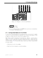
Reading the Boundary Mesh
. . . . . . . . . . . . . . . . . . . . . . . .
4-2
4.3
Examining the Boundary Mesh . . . . . . . . . . . . . . . . . . . . . . .
4-3
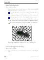
4.4
Generating the Interior Mesh . . . . . . . . . . . . . . . . . . . . . . . .
4-5
4.5
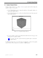
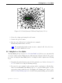
Displaying the Mesh . . . . . . . . . . . . . . . . . . . . . . . . . . . . .
4-6
4.6
Reporting the Mesh Statistics . . . . . . . . . . . . . . . . . . . . . . . .
4-8
4.7
Checking the Mesh . . . . . . . . . . . . . . . . . . . . . . . . . . . . . . 4-12
4.8
Saving the Mesh and Exiting TGrid . . . . . . . . . . . . . . . . . . . . . 4-12
5 Text User Interface
5.1
TOC-2
5-1
Text Menu System . . . . . . . . . . . . . . . . . . . . . . . . . . . . . .
5-1
5.1.1
5-3
Command Abbreviation . . . . . . . . . . . . . . . . . . . . . . .
c ANSYS, Inc. April 15, 2008
CONTENTS
5.1.2
Scheme Evaluation . . . . . . . . . . . . . . . . . . . . . . . . . .
5-4
5.1.3
Aliases . . . . . . . . . . . . . . . . . . . . . . . . . . . . . . . .
5-4
Text Prompt System . . . . . . . . . . . . . . . . . . . . . . . . . . . . .
5-4
5.2.1
Numbers . . . . . . . . . . . . . . . . . . . . . . . . . . . . . . .
5-5
5.2.2
Booleans . . . . . . . . . . . . . . . . . . . . . . . . . . . . . . .
5-5
5.2.3
Strings . . . . . . . . . . . . . . . . . . . . . . . . . . . . . . . .
5-5
5.2.4
Symbols
. . . . . . . . . . . . . . . . . . . . . . . . . . . . . . .
5-6
5.2.5
Filenames . . . . . . . . . . . . . . . . . . . . . . . . . . . . . . .
5-6
5.2.6
Lists
. . . . . . . . . . . . . . . . . . . . . . . . . . . . . . . . .
5-7
5.2.7
Evaluation . . . . . . . . . . . . . . . . . . . . . . . . . . . . . .
5-8
5.2.8
Default Value Binding . . . . . . . . . . . . . . . . . . . . . . . .
5-8
5.3
Interrupts . . . . . . . . . . . . . . . . . . . . . . . . . . . . . . . . . . .
5-8
5.4
System Commands . . . . . . . . . . . . . . . . . . . . . . . . . . . . . .
5-9
5.5
Text Menu Input from Character Strings . . . . . . . . . . . . . . . . . . 5-10
5.6
Using the Text Interface Help System
5.2
. . . . . . . . . . . . . . . . . . . 5-11
6 File Types
6.1
6-1
. . . . . . . . . . . . . . . . . . . . . . . . . . . . . . . . . .
6-1
6.1.1
Reading Boundary Mesh Files . . . . . . . . . . . . . . . . . . .
6-2
6.1.2
Reading TGrid Mesh Files . . . . . . . . . . . . . . . . . . . . . .
6-2
6.1.3
Appending Mesh Files . . . . . . . . . . . . . . . . . . . . . . . .
6-3
6.1.4
Writing Mesh Files . . . . . . . . . . . . . . . . . . . . . . . . . .
6-4
6.1.5
Writing Boundary Mesh Files . . . . . . . . . . . . . . . . . . . .
6-5
Compressed Files . . . . . . . . . . . . . . . . . . . . . . . . . . . . . . .
6-6
6.2.1
Reading Compressed Files . . . . . . . . . . . . . . . . . . . . . .
6-6
6.2.2
Writing Compressed Files . . . . . . . . . . . . . . . . . . . . . .
6-7
6.3
Reading Scheme Source Files . . . . . . . . . . . . . . . . . . . . . . . .
6-7
6.4
Journal Files . . . . . . . . . . . . . . . . . . . . . . . . . . . . . . . . .
6-8
6.4.1
6-8
6.2
Mesh Files
Using the GUI . . . . . . . . . . . . . . . . . . . . . . . . . . . .
c ANSYS, Inc. April 15, 2008
TOC-3
CONTENTS
6.4.2
6.5
6.6
6.7
6.8
6.9
Using Text Commands . . . . . . . . . . . . . . . . . . . . . . .
6-9
Transcript Files . . . . . . . . . . . . . . . . . . . . . . . . . . . . . . . .
6-9
6.5.1
Using the GUI . . . . . . . . . . . . . . . . . . . . . . . . . . . .
6-9
6.5.2
Using Text Commands . . . . . . . . . . . . . . . . . . . . . . .
6-9
Domain Files . . . . . . . . . . . . . . . . . . . . . . . . . . . . . . . . . 6-10
6.6.1
Reading Domain Files . . . . . . . . . . . . . . . . . . . . . . . . 6-10
6.6.2
Writing Domain Files . . . . . . . . . . . . . . . . . . . . . . . . 6-10
Importing Files . . . . . . . . . . . . . . . . . . . . . . . . . . . . . . . . 6-11
6.7.1
Importing Mesh Files Generated by Third-Party Packages . . . . 6-11
6.7.2
Importing FIDAP Neutral Mesh Files . . . . . . . . . . . . . . . . 6-14
6.7.3
Importing GAMBIT Neutral Mesh Files . . . . . . . . . . . . . . 6-14
6.7.4
Grid Import Filter Options . . . . . . . . . . . . . . . . . . . . . 6-14
Exporting Files . . . . . . . . . . . . . . . . . . . . . . . . . . . . . . . . 6-16
6.8.1
Exporting HYPERMESH Files . . . . . . . . . . . . . . . . . . . . 6-16
6.8.2
Exporting NASTRAN Files . . . . . . . . . . . . . . . . . . . . . 6-16
6.8.3
Exporting PATRAN Files . . . . . . . . . . . . . . . . . . . . . . 6-16
6.8.4
Exporting ANSYS and STL Files . . . . . . . . . . . . . . . . . . 6-17
Saving Hardcopy Files . . . . . . . . . . . . . . . . . . . . . . . . . . . . 6-17
6.9.1
Using the Hardcopy Panel . . . . . . . . . . . . . . . . . . . . . . 6-17
6.9.2
The Hardcopy Panel . . . . . . . . . . . . . . . . . . . . . . . . . 6-22
6.9.3
Text Interface for Saving Hardcopy Files . . . . . . . . . . . . . . 6-23
6.10 Saving the Panel Layout . . . . . . . . . . . . . . . . . . . . . . . . . . . 6-24
6.11 The .tgrid File . . . . . . . . . . . . . . . . . . . . . . . . . . . . . . . 6-25
6.12 Exiting TGrid . . . . . . . . . . . . . . . . . . . . . . . . . . . . . . . . . 6-25
7 Manipulating the Boundary Mesh
7.1
TOC-4
7-1
Manipulating Boundary Nodes . . . . . . . . . . . . . . . . . . . . . . .
7-2
7.1.1
Free and Isolated Nodes . . . . . . . . . . . . . . . . . . . . . . .
7-2
7.1.2
The Merge Boundary Nodes Panel . . . . . . . . . . . . . . . . . .
7-3
c ANSYS, Inc. April 15, 2008
CONTENTS
7.1.3
7.2
7.3
7.4
7.5
7.6
7.7
Text Commands for Manipulating Boundary Nodes
. . . . . . .
7-5
Intersecting Boundary Zones . . . . . . . . . . . . . . . . . . . . . . . .
7-6
7.2.1
Intersect . . . . . . . . . . . . . . . . . . . . . . . . . . . . . . .
7-6
7.2.2
Join . . . . . . . . . . . . . . . . . . . . . . . . . . . . . . . . . .
7-7
7.2.3
Stitch . . . . . . . . . . . . . . . . . . . . . . . . . . . . . . . . .
7-9
7.2.4
Using the Intersect Boundary Zones Panel . . . . . . . . . . . . . 7-10
7.2.5
The Intersect Boundary Zones Panel . . . . . . . . . . . . . . . . . 7-11
7.2.6
Text Commands for Boundary Intersection . . . . . . . . . . . . 7-13
Modifying the Boundary Mesh . . . . . . . . . . . . . . . . . . . . . . . 7-15
7.3.1
Using the Modify Boundary Panel . . . . . . . . . . . . . . . . . . 7-15
7.3.2
Operations Performed: Modify Boundary Panel . . . . . . . . . . 7-16
7.3.3
The Modify Boundary Panel . . . . . . . . . . . . . . . . . . . . . 7-23
7.3.4
Text Commands for Boundary Modification . . . . . . . . . . . . 7-29
Improving Boundary Surfaces . . . . . . . . . . . . . . . . . . . . . . . . 7-32
7.4.1
Improving the Boundary Surface Quality . . . . . . . . . . . . . 7-32
7.4.2
Smoothing the Boundary Surface . . . . . . . . . . . . . . . . . . 7-32
7.4.3
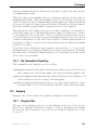
Swapping Face Edges . . . . . . . . . . . . . . . . . . . . . . . . 7-32
7.4.4
The Boundary Improve Panel . . . . . . . . . . . . . . . . . . . . 7-33
7.4.5
Text Commands for Improving Boundary Surfaces . . . . . . . . 7-35
Refining the Boundary Mesh . . . . . . . . . . . . . . . . . . . . . . . . 7-36
7.5.1
Procedure for Refining Boundary Zone(s) . . . . . . . . . . . . . 7-36
7.5.2
The Refine Boundary Zones Panel . . . . . . . . . . . . . . . . . . 7-38
7.5.3
Text Commands for Boundary Zone Refinement . . . . . . . . . 7-42
Creating and Modifying Features . . . . . . . . . . . . . . . . . . . . . . 7-42
7.6.1
Creating Edge Loops . . . . . . . . . . . . . . . . . . . . . . . . 7-43
7.6.2
Modifying Edge Loops . . . . . . . . . . . . . . . . . . . . . . . . 7-47
7.6.3
The Feature Modify Panel . . . . . . . . . . . . . . . . . . . . . . 7-50
7.6.4
Text Commands for Creating and Modifying Features . . . . . . 7-53
Remeshing Boundary Zones . . . . . . . . . . . . . . . . . . . . . . . . . 7-54
c ANSYS, Inc. April 15, 2008
TOC-5
CONTENTS
7.8
7.7.1
Creating Edge Loops . . . . . . . . . . . . . . . . . . . . . . . . 7-54
7.7.2
Modifying Edge Loops . . . . . . . . . . . . . . . . . . . . . . . . 7-55
7.7.3
Remeshing Surface Zones . . . . . . . . . . . . . . . . . . . . . . 7-55
7.7.4
Remeshing Zones Using the Surface Retriangulation Panel . . . . 7-56
7.7.5
The Surface Retriangulation Panel . . . . . . . . . . . . . . . . . . 7-57
7.7.6
Text Commands for Remeshing . . . . . . . . . . . . . . . . . . . 7-59
Faceted Stitching of Boundary Zones . . . . . . . . . . . . . . . . . . . . 7-61
7.8.1
7.9
The Faceted Stitch Panel . . . . . . . . . . . . . . . . . . . . . . 7-62
Triangulating Boundary Zones . . . . . . . . . . . . . . . . . . . . . . . 7-63
7.9.1
The Triangulate Zones Panel . . . . . . . . . . . . . . . . . . . . . 7-63
7.10 Separating Boundary Zones . . . . . . . . . . . . . . . . . . . . . . . . . 7-64
7.10.1
Methods for Separating Face Zones . . . . . . . . . . . . . . . . . 7-64
7.10.2
The Separate Face Zones Panel . . . . . . . . . . . . . . . . . . . 7-68
7.10.3
Text Commands for Separating Face Zones . . . . . . . . . . . . 7-70
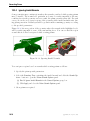
7.11 Projecting Boundary Zones . . . . . . . . . . . . . . . . . . . . . . . . . 7-70
7.11.1
The Project Face Zone Panel . . . . . . . . . . . . . . . . . . . . 7-71
7.11.2
Text Commands for Projecting Boundary Zones . . . . . . . . . 7-72
7.12 Creating Groups . . . . . . . . . . . . . . . . . . . . . . . . . . . . . . . 7-72
7.12.1
The User Defined Groups Panel . . . . . . . . . . . . . . . . . . . 7-73
7.12.2
Text Commands for User-Defined Groups . . . . . . . . . . . . . 7-74
7.13 Manipulating Boundary Zones . . . . . . . . . . . . . . . . . . . . . . . . 7-75
7.13.1
The Manage Face Zones Panel . . . . . . . . . . . . . . . . . . . 7-75
7.13.2
Text Commands for Manipulating Boundary Zones . . . . . . . . 7-78
7.14 Creating Surfaces . . . . . . . . . . . . . . . . . . . . . . . . . . . . . . . 7-79
TOC-6
7.14.1
Creating a Bounding Box . . . . . . . . . . . . . . . . . . . . . . 7-79
7.14.2
Creating a Planar Surface Mesh . . . . . . . . . . . . . . . . . . 7-82
7.14.3
Creating a Cylinder . . . . . . . . . . . . . . . . . . . . . . . . . 7-86
7.14.4
Creating a Swept Surface . . . . . . . . . . . . . . . . . . . . . . 7-88
7.14.5
Creating Periodic Boundaries . . . . . . . . . . . . . . . . . . . . 7-90
c ANSYS, Inc. April 15, 2008
CONTENTS
7.14.6
Text Commands for Creating Surfaces . . . . . . . . . . . . . . . 7-92
7.15 Additional Boundary Mesh Text Commands . . . . . . . . . . . . . . . . 7-92
8 Wrapping Boundaries
8.1
8-1
The Boundary Wrapper . . . . . . . . . . . . . . . . . . . . . . . . . . .
8-1
8.1.1
. . . . . . . . . . . . . . . . . . . . . .
8-2
8.2
The Wrapping Process . . . . . . . . . . . . . . . . . . . . . . . . . . . .
8-2
8.3
Examining and Repairing the Input Geometry . . . . . . . . . . . . . . .
8-4
8.4
Initializing the Cartesian Grid . . . . . . . . . . . . . . . . . . . . . . . .
8-6
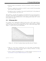
8.5
Examining the Cartesian Grid for Leakages . . . . . . . . . . . . . . . . 8-11
Applications of Wrapper
8.5.1
Automatic Leak Detection . . . . . . . . . . . . . . . . . . . . . 8-11
8.5.2
Manual Leak Detection . . . . . . . . . . . . . . . . . . . . . . . 8-12
8.6
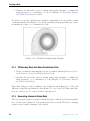
Extracting the Wrapper Surface . . . . . . . . . . . . . . . . . . . . . . . 8-16
8.7
Checking the Quality of the Wrapper Surface . . . . . . . . . . . . . . . 8-18
8.8
Post Wrapping Improvement Operations . . . . . . . . . . . . . . . . . . 8-18
8.9
8.8.1
Coarsening the Wrapper Surface . . . . . . . . . . . . . . . . . . 8-19
8.8.2
Post Wrap Options . . . . . . . . . . . . . . . . . . . . . . . . . 8-20
8.8.3
Zone Options . . . . . . . . . . . . . . . . . . . . . . . . . . . . . 8-27
8.8.4
Expert Options
. . . . . . . . . . . . . . . . . . . . . . . . . . . 8-29
The Boundary Wrapper Panel . . . . . . . . . . . . . . . . . . . . . . . . 8-33
8.9.1
The Wrapper Refinement Region Panel . . . . . . . . . . . . . . . 8-44
8.9.2
The Pan Regions Panel . . . . . . . . . . . . . . . . . . . . . . . 8-45
8.9.3
The Trace Path Panel . . . . . . . . . . . . . . . . . . . . . . . . 8-46
8.10 Text Commands for the Wrapper . . . . . . . . . . . . . . . . . . . . . . 8-47
9 Creating a Mesh
9.1
9-1
Choosing the Meshing Strategy . . . . . . . . . . . . . . . . . . . . . . .
9-1
9.1.1
3D Boundary Mesh Containing Only Triangular Faces . . . . . .
9-2
9.1.2
3D Boundary Mesh . . . . . . . . . . . . . . . . . . . . . . . . .
9-3
9.1.3
2D Boundary Mesh . . . . . . . . . . . . . . . . . . . . . . . . .
9-5
c ANSYS, Inc. April 15, 2008
TOC-7
CONTENTS
9.2
9.1.4
2D Boundary Mesh with Some Quadrilateral Cells . . . . . . . .
9-6
9.1.5
Generating a Hexcore Volume Mesh . . . . . . . . . . . . . . . .
9-6
9.1.6
Additional Meshing Tasks . . . . . . . . . . . . . . . . . . . . . .
9-7
9.1.7
Inserting Isolated Nodes into a Tri or Tet Mesh . . . . . . . . . .
9-9
Using the Auto Mesh Option . . . . . . . . . . . . . . . . . . . . . . . . . 9-11
9.2.1
9.3
9.4
9.5
The Auto Mesh Panel . . . . . . . . . . . . . . . . . . . . . . . . 9-12
Generating Pyramids . . . . . . . . . . . . . . . . . . . . . . . . . . . . . 9-13
9.3.1
Creating Pyramids . . . . . . . . . . . . . . . . . . . . . . . . . . 9-14
9.3.2
Zones Created During Pyramid Generation . . . . . . . . . . . . 9-16
9.3.3
The Pyramids Panel . . . . . . . . . . . . . . . . . . . . . . . . . 9-16
9.3.4
Text Interface for Generating Pyramids . . . . . . . . . . . . . . 9-20
9.3.5
Pyramid Meshing Problems . . . . . . . . . . . . . . . . . . . . . 9-20
Creating a Non-Conformal Interface . . . . . . . . . . . . . . . . . . . . 9-22
9.4.1
The Non Conformals Panel
. . . . . . . . . . . . . . . . . . . . . 9-22
9.4.2
Text Interface for Creating a Non-Conformal Interface . . . . . . 9-24
Creating a Heat Exchanger Zone . . . . . . . . . . . . . . . . . . . . . . 9-24
9.5.1
The Heat Exchanger Mesh Panel . . . . . . . . . . . . . . . . . . 9-25
10 Generating Prisms
10-1
10.1 Overview . . . . . . . . . . . . . . . . . . . . . . . . . . . . . . . . . . . 10-1
10.2 Procedure for Generating Prisms . . . . . . . . . . . . . . . . . . . . . . 10-2
10.3 Prism Meshing Options . . . . . . . . . . . . . . . . . . . . . . . . . . . 10-5
10.3.1
Growing Prisms Simultaneously from Multiple Zones . . . . . . . 10-5
10.3.2
Growing Prisms on a Two-Sided Wall . . . . . . . . . . . . . . . 10-6
10.3.3
Detecting Proximity and Collision . . . . . . . . . . . . . . . . . 10-7
10.3.4
Ignoring Invalid Normals . . . . . . . . . . . . . . . . . . . . . . 10-10
10.3.5
Preserving Orthogonality . . . . . . . . . . . . . . . . . . . . . . 10-11
10.4 Zones Created During Prism Generation . . . . . . . . . . . . . . . . . . 10-12
10.5 How TGrid Builds Prisms . . . . . . . . . . . . . . . . . . . . . . . . . . 10-12
TOC-8
c ANSYS, Inc. April 15, 2008
CONTENTS
10.6 Using Adjacent Zones as the Sides of Prisms . . . . . . . . . . . . . . . . 10-14
10.7 Direction Vectors . . . . . . . . . . . . . . . . . . . . . . . . . . . . . . . 10-17
10.8 Offset Distances . . . . . . . . . . . . . . . . . . . . . . . . . . . . . . . 10-19
10.9 Improving Prism Quality
. . . . . . . . . . . . . . . . . . . . . . . . . . 10-22
10.9.1
Edge Swapping and Smoothing . . . . . . . . . . . . . . . . . . . 10-22
10.9.2
Node Smoothing . . . . . . . . . . . . . . . . . . . . . . . . . . . 10-22
10.9.3
Improving Warp . . . . . . . . . . . . . . . . . . . . . . . . . . . 10-23
10.10 The Prisms Panel . . . . . . . . . . . . . . . . . . . . . . . . . . . . . . . 10-24
10.10.1 The Prisms Growth Options Panel . . . . . . . . . . . . . . . . . . 10-32
10.11 Text Interface for Generating Prisms . . . . . . . . . . . . . . . . . . . . 10-33
10.12 Prism Meshing Problems . . . . . . . . . . . . . . . . . . . . . . . . . . . 10-39
11 Generating Triangular/Tetrahedral Meshes
11-1
11.1 Automatically Creating a Tri or Tet Mesh . . . . . . . . . . . . . . . . . 11-2
11.1.1
Automatic Meshing Procedure for Tri/Tet Meshes . . . . . . . . 11-2
11.1.2
Using the Auto Mesh Tool . . . . . . . . . . . . . . . . . . . . . . 11-4
11.1.3
Automatic Meshing of Multiple Cell Zones . . . . . . . . . . . . 11-4
11.1.4
Automatic Meshing for Hybrid Meshes . . . . . . . . . . . . . . . 11-5
11.1.5
Further Mesh Improvements . . . . . . . . . . . . . . . . . . . . 11-6
11.2 Manually Creating a Tri or Tet Mesh . . . . . . . . . . . . . . . . . . . . 11-6
11.2.1
Manual Meshing Procedure for Tri/Tet Meshes . . . . . . . . . . 11-6
11.3 Initializing the Tri/Tet Mesh . . . . . . . . . . . . . . . . . . . . . . . . 11-10
11.3.1
Using the Tri/Tet Panel . . . . . . . . . . . . . . . . . . . . . . . 11-10
11.3.2
Text Commands for Initializing the Mesh . . . . . . . . . . . . . 11-11
11.4 Refining the Tri/Tet Mesh . . . . . . . . . . . . . . . . . . . . . . . . . . 11-12
11.4.1
Using Local Refinement Regions . . . . . . . . . . . . . . . . . . 11-13
11.4.2
Using the Tri/Tet Panel . . . . . . . . . . . . . . . . . . . . . . . 11-14
11.4.3
Text Commands for Setting Refinement Controls . . . . . . . . . 11-15
11.5 The Tri/Tet Panel . . . . . . . . . . . . . . . . . . . . . . . . . . . . . . 11-18
c ANSYS, Inc. April 15, 2008
TOC-9
CONTENTS
11.5.1
The Tri/Tet Init Controls Panel . . . . . . . . . . . . . . . . . . . 11-20
11.5.2
The Tri/Tet Refine Controls Panel . . . . . . . . . . . . . . . . . . 11-21
11.5.3
The Tri/Tet Refinement Region Panel . . . . . . . . . . . . . . . . 11-23
11.6 Additional Text Commands for Tri/Tet Mesh Generation . . . . . . . . . 11-24
11.7 Common Tri/Tet Meshing Problems . . . . . . . . . . . . . . . . . . . . 11-25
12 Generating the Hexcore Mesh
12-1
12.1 Automatic Hexcore Meshing Procedure . . . . . . . . . . . . . . . . . . . 12-1
12.2 Manual Hexcore Meshing Procedure . . . . . . . . . . . . . . . . . . . . 12-2
12.3 Controlling Hexcore Parameters . . . . . . . . . . . . . . . . . . . . . . . 12-3
12.3.1
Keep Outer Domain . . . . . . . . . . . . . . . . . . . . . . . . . 12-3
12.3.2
Hexcore Upto Boundaries . . . . . . . . . . . . . . . . . . . . . . 12-4
12.3.3
Only Hexcore . . . . . . . . . . . . . . . . . . . . . . . . . . . . . 12-5
12.3.4
Maximum Cell Length . . . . . . . . . . . . . . . . . . . . . . . . 12-6
12.3.5
Buffer Layers . . . . . . . . . . . . . . . . . . . . . . . . . . . . . 12-6
12.3.6
Peel Layers . . . . . . . . . . . . . . . . . . . . . . . . . . . . . . 12-7
12.3.7
Local Refinement Regions . . . . . . . . . . . . . . . . . . . . . . 12-8
12.4 The Hexcore Panel . . . . . . . . . . . . . . . . . . . . . . . . . . . . . . 12-9
12.4.1
The Outer Box Zones Panel . . . . . . . . . . . . . . . . . . . . . 12-11
12.4.2
The Hexcore Refinement Region Panel . . . . . . . . . . . . . . . 12-12
12.5 Text Commands for Hexcore Meshing . . . . . . . . . . . . . . . . . . . 12-13
13 Improving the Mesh
13-1
13.1 Smoothing Nodes . . . . . . . . . . . . . . . . . . . . . . . . . . . . . . . 13-2
13.1.1
Laplacian Smoothing . . . . . . . . . . . . . . . . . . . . . . . . 13-2
13.1.2
Variational Smoothing . . . . . . . . . . . . . . . . . . . . . . . . 13-2
13.1.3
Skewness-Based Smoothing . . . . . . . . . . . . . . . . . . . . . 13-2
13.1.4
Text Commands for Smoothing . . . . . . . . . . . . . . . . . . . 13-3
13.2 Swapping . . . . . . . . . . . . . . . . . . . . . . . . . . . . . . . . . . . 13-3
13.2.1
TOC-10
Triangular Grids . . . . . . . . . . . . . . . . . . . . . . . . . . . 13-3
c ANSYS, Inc. April 15, 2008
CONTENTS
13.2.2
Tetrahedral Grids . . . . . . . . . . . . . . . . . . . . . . . . . . 13-4
13.2.3
Text Interface for Smoothing and Swapping . . . . . . . . . . . . 13-5
13.3 Improving the Mesh . . . . . . . . . . . . . . . . . . . . . . . . . . . . . 13-5
13.4 Removing Slivers from a Tetrahedral Mesh . . . . . . . . . . . . . . . . . 13-6
13.4.1
Automatic Sliver Removal . . . . . . . . . . . . . . . . . . . . . . 13-7
13.4.2
Removing Slivers Manually . . . . . . . . . . . . . . . . . . . . . 13-7
13.4.3
Text Interface for Sliver Removal . . . . . . . . . . . . . . . . . . 13-9
13.5 The Tri/Tet Improve Panel . . . . . . . . . . . . . . . . . . . . . . . . . . 13-10
13.6 Modifying Cells . . . . . . . . . . . . . . . . . . . . . . . . . . . . . . . . 13-13
13.6.1
Using the Modify Cells Panel . . . . . . . . . . . . . . . . . . . . 13-13
13.6.2
The Modify Cells Panel . . . . . . . . . . . . . . . . . . . . . . . 13-16
13.6.3
Text Commands for Modifying Cell Zones . . . . . . . . . . . . . 13-18
13.7 Moving Nodes
. . . . . . . . . . . . . . . . . . . . . . . . . . . . . . . . 13-19
13.7.1
Automatic Correction . . . . . . . . . . . . . . . . . . . . . . . . 13-19
13.7.2
Semi-Automatic Correction . . . . . . . . . . . . . . . . . . . . . 13-20
13.7.3
The Auto Node Move Panel . . . . . . . . . . . . . . . . . . . . . 13-21
13.7.4
Text Commands for Moving Nodes . . . . . . . . . . . . . . . . . 13-22
13.8 Cavity Remeshing . . . . . . . . . . . . . . . . . . . . . . . . . . . . . . 13-23
13.8.1
The Cavity Remesh Panel . . . . . . . . . . . . . . . . . . . . . . 13-26
13.8.2
Text Commands for Cavity Remeshing
. . . . . . . . . . . . . . 13-27
13.9 Manipulating Cell Zones . . . . . . . . . . . . . . . . . . . . . . . . . . . 13-27
13.9.1
Active Zones and Cell Types . . . . . . . . . . . . . . . . . . . . 13-27
13.9.2
Copying and Moving Cell Zones . . . . . . . . . . . . . . . . . . 13-28
13.9.3
The Manage Cell Zones Panel . . . . . . . . . . . . . . . . . . . . 13-29
13.9.4
Text Commands for Manipulating Cell Zones . . . . . . . . . . . 13-32
13.10 Using Domains to Group and Mesh Boundary Faces . . . . . . . . . . . 13-33
13.10.1 Using Domains . . . . . . . . . . . . . . . . . . . . . . . . . . . . 13-34
13.10.2 Defining Domains . . . . . . . . . . . . . . . . . . . . . . . . . . 13-34
13.10.3 The Domains Panel . . . . . . . . . . . . . . . . . . . . . . . . . 13-35
c ANSYS, Inc. April 15, 2008
TOC-11
CONTENTS
13.10.4 Text Commands for Domains . . . . . . . . . . . . . . . . . . . . 13-37
13.11 Checking the Mesh . . . . . . . . . . . . . . . . . . . . . . . . . . . . . . 13-37
13.12 Clearing the Mesh . . . . . . . . . . . . . . . . . . . . . . . . . . . . . . 13-38
14 Examining the Mesh
14-1
14.1 Displaying the Grid . . . . . . . . . . . . . . . . . . . . . . . . . . . . . 14-2
14.1.1
Generating the Grid Display . . . . . . . . . . . . . . . . . . . . 14-2
14.1.2
Grid Display Options . . . . . . . . . . . . . . . . . . . . . . . . 14-3
14.1.3
The Display Grid Panel . . . . . . . . . . . . . . . . . . . . . . . . 14-4
14.1.4
Text Commands for Displaying the Grid . . . . . . . . . . . . . . 14-11
14.1.5
The Grid Colors Panel . . . . . . . . . . . . . . . . . . . . . . . . 14-13
14.1.6
Text Commands for Grid Colors . . . . . . . . . . . . . . . . . . 14-14
14.1.7
The Style Attributes Panel . . . . . . . . . . . . . . . . . . . . . . 14-15
14.1.8
Text Commands for Style Attributes . . . . . . . . . . . . . . . . 14-17
14.2 Checking Face Distribution . . . . . . . . . . . . . . . . . . . . . . . . . 14-17
14.2.1
The Face Distribution Panel . . . . . . . . . . . . . . . . . . . . . 14-18
14.2.2
Face Distribution Text Interface . . . . . . . . . . . . . . . . . . 14-20
14.3 Checking Cell Distribution . . . . . . . . . . . . . . . . . . . . . . . . . . 14-20
14.3.1
The Cell Distribution Panel . . . . . . . . . . . . . . . . . . . . . 14-21
14.3.2
Cell Distribution Text Interface . . . . . . . . . . . . . . . . . . . 14-22
14.4 Modifying the Attributes of the Plot Axes . . . . . . . . . . . . . . . . . 14-22
14.4.1
The Axes - Histogram Panel . . . . . . . . . . . . . . . . . . . . . 14-23
14.4.2
Text Interface for Modifying Axes Attributes . . . . . . . . . . . 14-25
14.5 Controlling Display Options . . . . . . . . . . . . . . . . . . . . . . . . . 14-25
14.5.1
The Display Options Panel . . . . . . . . . . . . . . . . . . . . . . 14-26
14.5.2
Text Commands for Controlling Display Options . . . . . . . . . 14-29
14.6 Modifying the View . . . . . . . . . . . . . . . . . . . . . . . . . . . . . 14-31
TOC-12
14.6.1
The Views Panel . . . . . . . . . . . . . . . . . . . . . . . . . . . 14-32
14.6.2
The Write Views Panel . . . . . . . . . . . . . . . . . . . . . . . . 14-33
c ANSYS, Inc. April 15, 2008
CONTENTS
14.6.3
The Mirror Planes Panel . . . . . . . . . . . . . . . . . . . . . . . 14-34
14.6.4
The Camera Parameters Panel . . . . . . . . . . . . . . . . . . . . 14-34
14.6.5
Text Commands for Modifying the View . . . . . . . . . . . . . . 14-36
14.7 Adding Lights . . . . . . . . . . . . . . . . . . . . . . . . . . . . . . . . . 14-37
14.7.1
The Lights Panel . . . . . . . . . . . . . . . . . . . . . . . . . . . 14-37
14.7.2
Text Commands for Adding Lights . . . . . . . . . . . . . . . . . 14-39
14.8 Describing a Scene . . . . . . . . . . . . . . . . . . . . . . . . . . . . . . 14-39
14.8.1
The Scene Description Panel . . . . . . . . . . . . . . . . . . . . . 14-39
14.8.2
Text Commands for Scene Description . . . . . . . . . . . . . . . 14-41
14.8.3
Changing the Display Properties . . . . . . . . . . . . . . . . . . 14-41
14.8.4
The Display Properties Panel . . . . . . . . . . . . . . . . . . . . 14-42
14.8.5
Transforming Geometric Objects in a Scene . . . . . . . . . . . . 14-43
14.8.6
The Bounding Frame Panel . . . . . . . . . . . . . . . . . . . . . 14-45
14.9 Controlling the Mouse Buttons . . . . . . . . . . . . . . . . . . . . . . . 14-46
14.9.1
The Mouse Buttons Panel . . . . . . . . . . . . . . . . . . . . . . 14-46
14.9.2
Text Commands for Selecting Mouse Buttons . . . . . . . . . . . 14-48
14.10 Controlling the Mouse Probe Functions
. . . . . . . . . . . . . . . . . . 14-48
14.10.1 The Mouse Probe Panel . . . . . . . . . . . . . . . . . . . . . . . 14-49
14.10.2 Text Commands for Mouse Probe Selection . . . . . . . . . . . . 14-50
14.11 Annotating the Display . . . . . . . . . . . . . . . . . . . . . . . . . . . 14-50
14.11.1 The Annotate Panel . . . . . . . . . . . . . . . . . . . . . . . . . 14-50
14.11.2 Text Commands for Text Annotation . . . . . . . . . . . . . . . 14-51
14.12 Shortcuts for Selecting Zones . . . . . . . . . . . . . . . . . . . . . . . . 14-52
14.12.1 The Zone Selection Helper Panel . . . . . . . . . . . . . . . . . . 14-52
15 Reporting Mesh Statistics
15-1
15.1 Reporting the Mesh Size . . . . . . . . . . . . . . . . . . . . . . . . . . . 15-1
15.1.1
The Report Mesh Size Panel . . . . . . . . . . . . . . . . . . . . . 15-1
15.1.2
Text Commands for Reporting Mesh Size . . . . . . . . . . . . . 15-2
c ANSYS, Inc. April 15, 2008
TOC-13
CONTENTS
15.2 Reporting Face Limits . . . . . . . . . . . . . . . . . . . . . . . . . . . . 15-3
15.2.1
The Report Face Limits Panel . . . . . . . . . . . . . . . . . . . . 15-3
15.2.2
Text Commands for Reporting Face Limits . . . . . . . . . . . . 15-5
15.3 Reporting Cell Limits . . . . . . . . . . . . . . . . . . . . . . . . . . . . 15-5
15.3.1
The Report Cell Limits Panel . . . . . . . . . . . . . . . . . . . . 15-5
15.3.2
Text Commands for Reporting Cell Limits . . . . . . . . . . . . 15-6
15.4 Reporting Boundary Cell Limits . . . . . . . . . . . . . . . . . . . . . . 15-6
15.4.1
The Report Boundary Cell Limits Panel . . . . . . . . . . . . . . . 15-7
15.4.2
Text Commands for Reporting Boundary Cell Limits . . . . . . . 15-8
15.5 Mesh Quality . . . . . . . . . . . . . . . . . . . . . . . . . . . . . . . . . 15-8
15.5.1
Quality Measures Available in TGrid . . . . . . . . . . . . . . . . 15-9
15.5.2
Specifying the Quality Measure . . . . . . . . . . . . . . . . . . . 15-13
15.5.3
Text Commands for Selecting the Quality Measure . . . . . . . . 15-15
15.6 Printing Grid Information . . . . . . . . . . . . . . . . . . . . . . . . . . 15-15
15.6.1
Boundary Node . . . . . . . . . . . . . . . . . . . . . . . . . . . 15-15
15.6.2
Node . . . . . . . . . . . . . . . . . . . . . . . . . . . . . . . . . 15-16
15.6.3
Boundary Face . . . . . . . . . . . . . . . . . . . . . . . . . . . . 15-16
15.6.4
Cell . . . . . . . . . . . . . . . . . . . . . . . . . . . . . . . . . . 15-17
15.6.5
Face . . . . . . . . . . . . . . . . . . . . . . . . . . . . . . . . . . 15-17
15.7 Additional Text Commands for Reporting . . . . . . . . . . . . . . . . . 15-18
A Importing Boundary and Volume Meshes
A-1
A.1 GAMBIT Meshes . . . . . . . . . . . . . . . . . . . . . . . . . . . . . . . A-1
A.2 TetraMesher Volume Mesh . . . . . . . . . . . . . . . . . . . . . . . . . . A-1
A.3 Meshes from Third-Party CAD Packages . . . . . . . . . . . . . . . . . . A-1
TOC-14
A.3.1
Using the fe2ram Filter to Convert Files . . . . . . . . . . . . . A-1
A.3.2
I-deas Universal Files . . . . . . . . . . . . . . . . . . . . . . . . . A-2
A.3.3
PATRAN Neutral Files . . . . . . . . . . . . . . . . . . . . . . . . A-4
A.3.4
ANSYS Files . . . . . . . . . . . . . . . . . . . . . . . . . . . . . A-5
c ANSYS, Inc. April 15, 2008
CONTENTS
A.3.5
ARIES Files . . . . . . . . . . . . . . . . . . . . . . . . . . . . . . A-6
A.3.6
NASTRAN Files . . . . . . . . . . . . . . . . . . . . . . . . . . . A-6
B Mesh File Format
B-1
B.1 Comment . . . . . . . . . . . . . . . . . . . . . . . . . . . . . . . . . . . B-1
B.2 Header . . . . . . . . . . . . . . . . . . . . . . . . . . . . . . . . . . . . . B-2
B.3 Dimensions . . . . . . . . . . . . . . . . . . . . . . . . . . . . . . . . . . B-2
B.4 Nodes . . . . . . . . . . . . . . . . . . . . . . . . . . . . . . . . . . . . . B-3
B.5 Periodic Shadow Faces . . . . . . . . . . . . . . . . . . . . . . . . . . . . B-4
B.6 Cells . . . . . . . . . . . . . . . . . . . . . . . . . . . . . . . . . . . . . . B-6
B.7 Faces . . . . . . . . . . . . . . . . . . . . . . . . . . . . . . . . . . . . . B-7
B.8 Face Tree . . . . . . . . . . . . . . . . . . . . . . . . . . . . . . . . . . . B-9
B.9 Cell Tree . . . . . . . . . . . . . . . . . . . . . . . . . . . . . . . . . . . B-9
B.10 Interface Face Parents . . . . . . . . . . . . . . . . . . . . . . . . . . . . B-10
B.11 Example Files . . . . . . . . . . . . . . . . . . . . . . . . . . . . . . . . . B-11
C Shortcut Keys
C-1
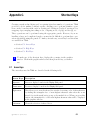
C.1 Arrow Keys . . . . . . . . . . . . . . . . . . . . . . . . . . . . . . . . . . C-1
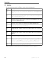
C.2 Help Keys . . . . . . . . . . . . . . . . . . . . . . . . . . . . . . . . . . . C-2
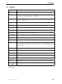
C.3 Hot Keys . . . . . . . . . . . . . . . . . . . . . . . . . . . . . . . . . . . C-3
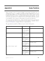
D Query Functions
D-1
D.1 Using Boolean Operations with Query Functions . . . . . . . . . . . . . D-3
D.2 Examples . . . . . . . . . . . . . . . . . . . . . . . . . . . . . . . . . . . D-4
E Tips
E-1
E.1
Reading Files . . . . . . . . . . . . . . . . . . . . . . . . . . . . . . . . . E-1
E.2
Writing Files . . . . . . . . . . . . . . . . . . . . . . . . . . . . . . . . . E-2
E.3
Saving Hard Copy Files . . . . . . . . . . . . . . . . . . . . . . . . . . . E-3
E.4
Importing Meshes . . . . . . . . . . . . . . . . . . . . . . . . . . . . . . E-4
E.5
Creating a Mesh . . . . . . . . . . . . . . . . . . . . . . . . . . . . . . . E-5
c ANSYS, Inc. April 15, 2008
TOC-15
CONTENTS
E.6
Grouping Elements . . . . . . . . . . . . . . . . . . . . . . . . . . . . . . E-5
E.7
Deleting Duplicate Nodes . . . . . . . . . . . . . . . . . . . . . . . . . . E-5
E.8
Manipulating the Boundary Mesh File . . . . . . . . . . . . . . . . . . . E-6
E.9
Examining the Mesh . . . . . . . . . . . . . . . . . . . . . . . . . . . . . E-7
E.10 Reporting Mesh Statistics . . . . . . . . . . . . . . . . . . . . . . . . . . E-7
E.11 Refining the Mesh . . . . . . . . . . . . . . . . . . . . . . . . . . . . . . E-8
E.12 Using the GUI . . . . . . . . . . . . . . . . . . . . . . . . . . . . . . . . E-10
TOC-16
c ANSYS, Inc. April 15, 2008
Using This Manual
The Contents of This Manual
The TGrid User’s Guide tells you what you need to know to use TGrid. Chapters 6
through 15 describe the menus that appear at the top of the TGrid window and explain
the use of the associated graphical user interface menu items and the text interface
menu items. The appendices contain information about importing boundary and volume
meshes, the mesh file format, tips, troubleshooting, and the shortcut keys and query
functions available in TGrid to make your task easier. At the end of the User’s Guide,
you will find a glossary, a bibliography, and the index.
i
Under U. S. and international copyright law, ANSYS, Inc. is unable to
distribute copies of the papers listed in the bibliography, other than those
published internally by ANSYS, Inc. Please use your library or a document
delivery service to obtain copies of copyrighted papers.
A brief description of what’s in each chapter follows:
• Chapter 1: Introduction to TGrid gives you an overview of unstructured grid generation and describes the way in whichTGrid interacts with other products.
• Chapter 2: Getting Started gives an overview of the problem setup steps. In this
chapter you will also find information about starting TGrid.
• Chapter 3: Graphical User Interface describes the using of the graphical user interface. It also explains how to use the TGrid on-line help system.
• Chapter 4: Sample Session presents a sample TGrid session that you can work
through at your own pace.
• Chapter 5: Text User Interface describes the use of the text interface and options
associated with it. See the separate Text Command List for information about
specific text interface commands.
• Chapter 6: File Types contains information about the files that TGrid can read and
write (including hardcopy files).
• Chapter 7: Manipulating the Boundary Mesh explains the need for a high-quality
boundary mesh and describes various options available to create such mesh.
c ANSYS, Inc. April 15, 2008
UTM-1
Using This Manual
• Chapter 8: Wrapping Boundaries contains information about creating a high-quality
boundary mesh starting from bad surface mesh using the surface wrapper tool.
• Chapter 9: Creating a Mesh describes the meshing strategy and creation of pyramids, non-conformals, and heat exchanger mesh.
• Chapter 10: Generating Prisms describes the procedure to create prism mesh. It
also explains how to deal with common problems that can be faced while creating
prisms.
• Chapter 11: Generating Triangular/Tetrahedral Meshes describes the meshing procedures for triangular and tetrahedral meshes.
• Chapter 12: Generating the Hexcore Mesh describes the procedure and options for
creating hexcore meshes.
• Chapter 13: Improving the Mesh describes the options available for improving the
quality of a volume mesh.
• Chapter 14: Examining the Mesh describes the methods available for checking the
mesh graphically.
• Chapter 15: Reporting Mesh Statistics describes methods for checking the mesh
diagnostically.
• Appendix A: Importing Boundary and Volume Meshes describes filters that you
can use to convert data from various software packages to a form that TGrid can
accept.
• Appendix B: Mesh File Format describes the format of the TGrid mesh file.
• Appendix C: Shortcut Keys lists all the hotkeys (shortcut keys) available in TGrid.
• Appendix D: Query Functions lists the query functions available in TGrid.
• Appendix E: Tips contains information on tips that will be useful to you while
working on TGrid.
The Contents of Other Manuals
In addition to this User’s Guide, there are two more manuals available to help you use
TGrid:
• The Tutorial Guide contains example problems. Each tutorial contains detailed
instructions on performing the tasks associated with it.
• The Text Command List provides a brief description of the commands in the
TGrid text interface.
UTM-2
c ANSYS, Inc. April 15, 2008
Using This Manual
How To Use This Manual
Depending on your familiarity with computational fluid dynamics (CFD) and the TGrid
software, you can use this manual in different ways.
For the Beginner
The suggested readings for the beginner are as follows:
• For information about how TGrid relates to and interacts with other products, or
about the motivation for unstructured grid generation, read Chapter 1: Introduction
to TGrid.
• To learn more about the user interface, read Chapters 3 and 5.
• To learn about reading and writing files, see Chapter 6: File Types.
• For information about checking and improving a boundary mesh, see Chapter 7: Manipulating the Boundary Mesh.
• To find out about the different types of meshes that TGrid can generate, the meshing
processes, and how to solve or avoid meshing problems, see Chapters 9—12.
• To learn about checking the quality of the mesh, see Chapters 14 and 15.
• To find out how to use the on-line help in TGrid, read Section 3.6: Using the GUI
Help System.
Depending on the characteristics of your particular problem, and the tools you want to
employ, use the table of contents and the indexes to find the relevant information.
For the Experienced User
If you are an experienced user who needs to look up specific information, there are
different tools that allow you to use the TGrid User’s Guide as a reference manual.
• The table of contents, lists topics that are discussed in a procedural order, enabling
you to find material relating to a particular procedural step.
• The Index, allows you to access information about a particular subject.
c ANSYS, Inc. April 15, 2008
UTM-3
Using This Manual
Typographical Conventions Used In This Manual
Several typographical conventions are used in the text of this manual to facilitate your
learning process.
• An informational icon (
• A warning icon (
) marks an important note.
) marks an important note or warning.
• Different type styles are used to indicate graphical user interface menu items and
text interface menu items (e.g., Display Grid panel, display/grid command).
• The text interface type style is also used when illustrating exactly what appears on
the screen or exactly what you need to type into a field in a panel.
• A mini flow chart is used to indicate the menu selections that lead you to a specific
panel. For example,
Display −→Grid...
indicates that the Grid... menu item can be selected from the Display pull-down
menu at the top of the TGrid console window.
The words surrounded by boxes invoke menus (or submenus) and the arrows point
from a specific menu toward the item you should select from that menu. In this
manual, mini flow charts usually precede a description of a panel or a screen illustration showing how to use the panel. They allow you to look up information
about a panel and quickly determine how to access it without having to search the
preceding material.
• The menu selections that will lead you to a particular panel are also indicated
(usually within a paragraph) using a “/”. For example, Display/Grid... tells you to
choose Grid... from the Display menu.
Contacting Technical Support
The support engineers can help you to plan your CFD modeling projects and to overcome
any difficulties you encounter while using TGrid. If you encounter difficulties we invite
you to call your support engineer for assistance. However, there are a few things that we
encourage you to do before calling:
• Read the section(s) of the manual containing information on the commands you
are trying to use or the type of problem you are trying to solve.
• Recall the exact steps you were following that led up to and caused the problem.
UTM-4
c ANSYS, Inc. April 15, 2008
Using This Manual
• Write down the exact error message that appeared, if any.
• For particularly difficult problems, save a transcript file of the TGrid session in
which the problem occurred. This is the best source that we can use to reproduce
the problem and thereby help to identify the cause.
c ANSYS, Inc. April 15, 2008
UTM-5
Using This Manual
UTM-6
c ANSYS, Inc. April 15, 2008
Chapter 1.
Introduction to TGrid
This chapter provides an introduction to TGrid, an explanation of its capabilities, and
instructions for starting TGrid.
• Section 1.1: Introduction
• Section 1.2: Program Structure
• Section 1.3: Program Capabilities
• Section 1.4: Accessing TGrid Manuals
1.1
Introduction
TGrid is a highly efficient, easy-to-use, unstructured grid generation program that can
handle grids of virtually unlimited size and complexity, consisting of triangular, tetrahedral, hexahedral, prismatic, or pyramidal cells.
Unstructured grid generation techniques couple basic geometric building blocks with
extensive geometric data to highly automate the grid generation process. In addition,
the generalized data structures used in these schemes permit the addition and removal
of cells to maximize accuracy and minimize memory and CPU requirements.
For input TGrid requires a discretized boundary mesh consisting of either nodes and
edges in 2D, or nodes and triangular/quadrilateral faces in 3D. TGrid contains a number
of tools for checking and repairing the boundary mesh to ensure a good starting point
for the mesh. A complete mesh can be generated from the boundary mesh automatically
or by exercising control of the process.
The user interface to TGrid is written in the Scheme language, which is a dialect of
LISP. Most features are accessible through the graphical interface or the interactive
menu interface. The advanced user can customize and enhance the interface by adding
or changing the Scheme functions.
c ANSYS, Inc. April 15, 2008
1-1
Introduction to TGrid
1.2
Program Structure
TGrid is part of the FLUENT package, which includes the following products:
• FLUENT, the solver.
• GAMBIT, the preprocessor for geometry modeling and mesh generation.
• TGrid, the additional preprocessor that can generate volume meshes from existing
boundary meshes.
• Filters (translators) for import of surface and volume meshes from CAD/CAE
packages such as ANSYS, I-deas, NASTRAN, PATRAN, and others.
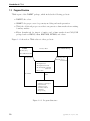
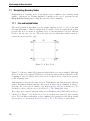
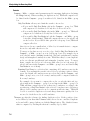
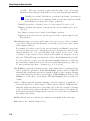
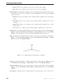
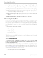
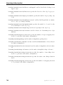
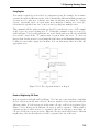
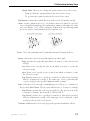
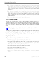
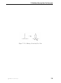
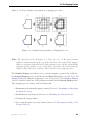
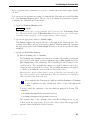
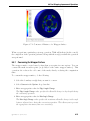
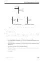
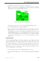
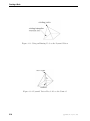
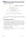
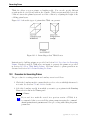
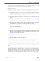
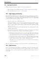
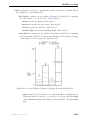
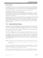
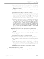
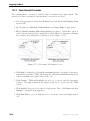
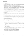
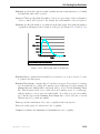
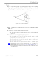
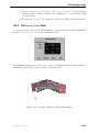
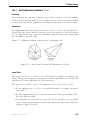
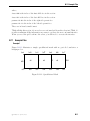
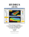
Figure 1.2.1 shows how TGrid relates to these products.
GAMBIT
Geometry / Mesh
Other CAD/CAE Packages
− Geometry set up
− 2D / 3D Mesh Generation
Boundary Mesh
TGrid
− 2D triangular mesh
Faceted geometry
Boundary and / or
Volume Mesh
− 3D triangular surface mesh
− 2D / 3D triangular / tetrahedral
hybrid mesh
− Hexcore mesh
2D / 3D Mesh
Mesh
FLUENT (V5 or later)
− Mesh import and adaption
− Physical models
− Material properties
− Boundary conditions
− Calculation
− Postprocessing
Figure 1.2.1: Program Structure
1-2
c ANSYS, Inc. April 15, 2008
1.3 Program Capabilities
You can use TGrid to generate a triangular, tetrahedral, hexcore, or hybrid volume mesh
from an existing boundary mesh.
To create a mesh in TGrid, first use a preprocessor (GAMBIT or a third-party CAD package) to create a boundary mesh in which the boundaries are defined by line segments
(2D) or triangular or quadrilateral facets (3D). To create tetrahedral, prismatic, or pyramidal cells, read the boundary mesh (and any hexahedral cells) into TGrid and continue
the mesh generation process there.
The first step in producing an unstructured grid is to define the shape of the domain
boundaries.
Surface grids created in CAD/CAE packages can be read into TGrid using the appropriate
menu item in the File/Import pull-down submenu (or the associated text commands), or
converted using the appropriate stand-alone grid filter.
When the grid generation is completed, you can read the 3D grid created by TGrid into
the solver. After a grid is read into the solver, the remaining operations are performed
there. These include setting boundary conditions, defining fluid properties, executing the
solution, and viewing and postprocessing the results.
1.3
Program Capabilities
TGrid is a robust and a highly automated unstructured volume mesh generator with the
following meshing capabilities:
• Generates triangles (tris) and quadrilaterals (quads) in 2D.
• Generates tets, hexcore, prisms, pyramids in 2D.
• Generates volume mesh that is accepted by FLUENT.
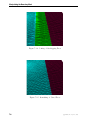
• Uses Delaunay triangulation method for tris/tets.
• Uses advancing layer method for prisms.
• Generates hexcore mesh.
• Has a robust boundary wrapper tool.
• Can export polyhedral cells.
• Has tools for checking, repairing, and improving boundary mesh to ensure a good
starting point for the mesh.
• Is capable of manipulating face/cell zones.
• Is flexible—it allows the most appropriate cell type to be used to generate the
volume mesh:
c ANSYS, Inc. April 15, 2008
1-3
Introduction to TGrid
– Tri/tet meshes are suitable for complex geometries.
– Hexcore meshes can combine the flexibility of tet, hex, and prism meshes with
smaller cell count.
• Hybrid meshes:
– Prism layers near walls allow proper boundary layer resolution.
– Allows flow alignments with grid lines.
– Generates smaller volume mesh with highly stretched prismatic elements.
• Non-conformal meshes:
– Suitable for parametric studies.
– Meshes generated separately can be glued together.
1.4
Accessing TGrid Manuals
The on-line help gives you access to the TGrid User’s Guide through HTML files. These
files can be viewed with any web browser.
To see the User’s Guide, select User’s Guide Contents... in the Help pull-down menu in
the TGrid GUI. This will open the User’s Guide contents page.
You can access the required information by using the Table of Contents that displays a
list of chapters, including all section and subsection titles. Each of these, is a link to the
corresponding chapter or section or subsection of the manual. You can also use the Index
to take you to the relevant section of the User’s Guide. For details on using GUI help
system, see Section 3.6: Using the GUI Help System.
1-4
c ANSYS, Inc. April 15, 2008
Chapter 2.
Getting Started
This chapter provides an overview of using TGrid and instructions for starting it.
• Section 2.1: Using TGrid
• Section 2.2: Starting TGrid
• Section 2.3: Starting Dual Process Build of TGrid
2.1
Using TGrid
Starting from a given boundary mesh (or a boundary mesh with some 2D quadrilateral
or 3D hexahedral cells), TGrid generates an unstructured triangular or tetrahedral (or
hybrid) grid. In 2D, the boundary mesh consists of nodes and straight edges, whereas in
3D, it consists of nodes and triangular and/or quadrilateral faces.
A boundary mesh file can be obtained from a number of sources including GAMBIT.
TGrid creates an interior mesh, from the boundary mesh and writes it to a new file. This
file can then be read into the solver, where the solution process and postprocessing occur.
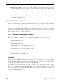
2.1.1 Grid Generation Steps
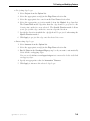
The basic steps for using TGrid are as follows:
1. Read a simple boundary mesh file or a boundary mesh containing some 2D quadrilateral or 3D hexahedral cells into TGrid.
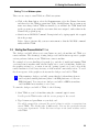
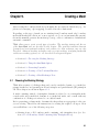
2. Examine the boundary mesh for topological problems such as free edges and duplicate nodes. When the boundary is topologically correct, you can check a 3D
surface mesh for poor face quality.
Many quality-related problems can be solved easily with edge swapping, but more
difficult problems may require direct manipulation of the faces and nodes.
3. Generate the volume mesh. You can do this automatically or by proceeding through
a series of steps.
• For hybrid grids, first generate prisms or pyramids, and then generate the
triangular or tetrahedral volume cells. If required, you can extend the computational domain by generating more prisms.
c ANSYS, Inc. April 15, 2008
2-1
Getting Started
• For grids containing only triangles or tetrahedra, you can either use the automatic mesh generation procedure, or perform each step yourself.
4. Check the mesh for problems (quality and location).
The presence of degenerate cells will prevent you from obtaining a solution, and
poor cells in critical areas will cause serious accuracy and convergence problems. If
such cells cannot be removed or improved, you will have to generate a new mesh
by modifying the boundary mesh and/or using different mesh parameters.
5. Write the mesh to a new file for input to the solver.
2.2
Starting TGrid
The installation process (described in a separate booklet) is designed to ensure that
the TGrid is installed properly so that the program can be launched when you follow the
appropriate instructions. If not, consult your computer systems manager or your support
engineer. The way you start TGrid will be different for UNIX and Windows systems.
Starting TGrid on UNIX system
To start TGrid, type tgrid 2d or tgrid 3d in the command line of an xterm window.
When TGrid starts, it will display a text window and the main menu bar. This is called
the console window.
If you start TGrid on UNIX systems without specifying 2d or 3d, press the return key to
see the following list of options:
TGrid version>
2d
3d
custom
executable
host
listen
custom prompts you for a version that is not in the menu, i.e., a version that is not
part of the standard distribution. You can also use it to add options to a standard
version name (e.g., custom "2d -option").
executable sets the name of the program to be run. The default is "tgrid". You can
use this option to give a full pathname if the executable is not in your search path
(e.g., executable "/Fluent.Inc/bin/tgrid").
host sets the machine and username on which TGrid is to be run. If necessary, you
will be prompted for a password in the window in which Cortex was started. The
default is to run on the same machine on which Cortex is running.
listen tells Cortex to wait a specified period of time for a TGrid session to start up
instead of starting TGrid itself.
2-2
c ANSYS, Inc. April 15, 2008
2.3 Starting Dual Process Build of TGrid
Starting TGrid on Windows system
There are two ways to start TGrid on a Windows system:
• Click on the Start button, select the Programs menu, select the Fluent.Inc menu,
and then select the TGrid program item. If the default Fluent.Inc program group
name was changed when TGrid was installed, you will find the TGrid menu item
in the program group with the new name that was assigned, rather than in the
Fluent.Inc program group.
• Start from an MS-DOS Command Prompt window by typing tgrid 2d or tgrid
3d at the prompt.
Before doing so, first modify your user environment so that the MS-DOS command
utility will find TGrid.
2.3
Starting Dual Process Build of TGrid
The dual process build allows you to run Cortex on your local machine and TGrid on a
remote machine. The advantage of using dual process build is faster response to graphic
actions performed when you use TGrid from a remote machine.
For example, if you are handling a big mesh (e.g., underhood mesh) and running TGrid
on a faster remote machine with only the display set to your local machine. In this case,
the graphics actions (e.g., zoom-in, zoom-out, opening a panel, etc.) can be slow if the
remote machine is located very far away or if the network connectivity is slow. To avoid
the slow response of the graphics actions, run the dual process build of TGrid.
i
When running a dual process build, ensure that the both machines (remote
and host) have similar platforms (either both IBM platforms or both nonIBM platforms). You can not use dual process build for IBM host machine
and non-IBM remote machine or vice versa.
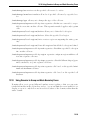
To start the dual process build of TGrid, do the following:
1. Start TGrid on your local machine using the command tgrid -serv.
It will open the TGrid window with the version prompt in the console.
2. Type listen and press Enter on your keyboard.
You will be prompted for a timeout (the period of time to wait for a connection from
remote TGrid). The default value is 300 seconds. You can also specify the timeout
as per your requirement. Utilize this time to login to the faster machine and to
start TGrid.
c ANSYS, Inc. April 15, 2008
2-3
Getting Started
3. Press Enter on your keyboard again.
A message will prompt you to start TGrid on remote machine with the following
arguments:
-cx host:p1:p2
where,
host is the name of the host (local) machine on which the Cortex is running on.
p1 and p2 are the two integers indicating the connecting port numbers that are used
to communicate information between the Cortex on the host machine and TGrid on
the remote machine.
4. Login to the remote machine and set the display to the host machine.
5. Start TGrid from remote machine using the following command:
tgrid version -cx host:p1:p2
Replace version by the version that you wish to run (2d or 3d). The host and
port numbers are displayed in the TGrid console window.
The GUI commands related to the File menu (e.g., reading file, importing file) and other
Select File dialogs do not work for dual process build. Therefore, use the TUI commands.
2.3.1
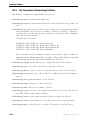
Startup Options
Before starting TGrid you can obtain information about the available releases. Type
tgrid -help in an xterm window (on UNIX systems) or the MS-DOS Command Prompt
window (on Windows systems).
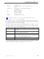
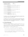
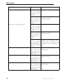
The options available are:
Usage: [version] [-help] [options]
options:
-cl
following argument passed to tgrid,
-cxarg
following argument passed to cortex,
-cx host:p1:p2 connect to the specified cortex process,
-driver [ gl | opengl | null | pex | sbx | x11 | xgl ],
sets the graphics driver (available
drivers vary by platform),
-env
show environment variables,
-g
run without gui or graphics,
-gu
run without gui,
-gr
run without graphics,
-help
this listing,
-i journal
read the specified journal file,
2-4
c ANSYS, Inc. April 15, 2008
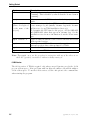
2.3 Starting Dual Process Build of TGrid
-n
-nocheck
-project x
-r
-rx
-v
-vx
version
i
no execute,
disable checks for valid license file and
server,
write project x start and end times to
license log,
list all releases,
specify release x,
list all versions,
specify version x,
if given, must be first.
On Windows systems, only -env, -gu (with restrictions), -help, -i
journal, -r, -rx, -v, and -vx are available.
The first three options are for specifying arguments for TGrid and Cortex. Cortex is a
process that provides the user interface and graphics for TGrid. When you start TGrid,
you actually start Cortex, which then starts TGrid.
On Windows systems, tgrid -gu will run TGrid keeping it in its iconified form. The
GUI will be available if you expand it. This option can be used in conjunction with the
-i journal option to run a job in background mode.
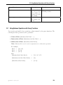
Options
-cx host:p1:p2
tgrid -driver
tgrid -env
tgrid -g
tgrid -gu
tgrid -gr
Description
Used only when you start TGrid manually (see Section 2.2: Starting TGrid).
Allows you to specify the graphics driver to be used in the TGrid
session (e.g., tgrid -driver xgl).
Lists all environment variables before running TGrid.
Runs Cortex without graphics and without the graphical user
interface. This option is useful if you are not on an X Window
display or if you want to submit a batch job.
Runs Cortex without the graphical user interface.
Runs Cortex without graphics.
To start TGrid and immediately read a journal file, enter the command tgrid -i journal,
replacing journal with the name of the journal file you want to read.
c ANSYS, Inc. April 15, 2008
2-5
Getting Started
Options
-nocheck
Description
Speeds up the startup by not checking to see if the license server
is running. This is useful if you know that the license daemon
is running.
-project x
Allows you to record CPU time for individual “projects” separately.
tgrid -project x
Extra information related to CPU time will be written to the
(where x is replaced license manager log file (usually license.log in the license
by the name of the subdirectory of your TGrid installation directory).
project)
To determine the CPU time for the project, add the USER CPU
and SYSTEM CPU values that appear in license.log. See the
installation notes for more information about the license manager.
tgrid version -r
Replaces version with the desired version and lists all releases
of the specified version.
tgrid -rx
Runs release x of TGrid. You may either specify a version or
wait and specify it later, when prompted by TGrid.
tgrid -v
Lists the available versions.
tgrid -vx
Runs version x of TGrid.
Note: Type tgrid -n or use the -n option in conjunction with any of the others to see
where the (specified) executable is without actually running it.
64-Bit Version
The 64-bit version of TGrid is required only when your problem size exceeds the 32-bit
process address space. Most problems with less than two million cells will fit within a
32-bit address space. To use the 64-bit version, add the -64 option to the command line
when starting the program.
2-6
c ANSYS, Inc. April 15, 2008
Chapter 3.
Graphical User Interface
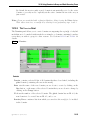
The graphical user interface (GUI) is made up of four main components: a console,
control panels, dialog boxes, and graphics windows. When you use the GUI, you will be
interacting with one of these components at all times.
This chapter describes the GUI components and explains the procedure to customize
the attributes of the GUI (including colors and text fonts) on UNIX systems, to better
match your platform environment. It also explains the procedure to use the help system
in TGrid.
The following sections are described in this chapter:
• Section 3.1: Console
• Section 3.2: Dialog Boxes
• Section 3.3: Panels
• Section 3.4: Graphics Display Windows
• Section 3.5: Customizing the GUI (UNIX Systems)
• Section 3.6: Using the GUI Help System
c ANSYS, Inc. April 15, 2008
3-1
Graphical User Interface
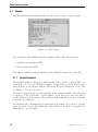
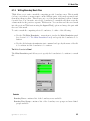
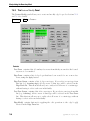
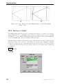
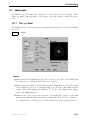
3.1
Console
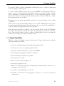
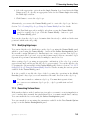
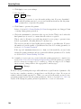
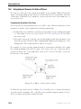
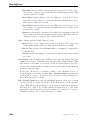
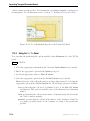
The TGrid Console is the main window that controls the execution of the program.
Figure 3.1.1: The Console
You can interact with TGrid through the Console in either of the following ways:
• graphical user interface (GUI)
• text user interface (TUI)
The Console contains a terminal emulator for the TUI and a menu bar for the GUI.
3.1.1
Terminal Emulator
The terminal emulator behaves in a similar manner as the “xterm” or other UNIX command shell tools, or to the MS-DOS Command Prompt window (on the Windows system). It allows you to interact with the TUI menu. For more information on the TUI,
see Chapter 5: Text User Interface.
All textual output from the program is printed in the terminal emulator, and all typing
is displayed on the bottom line. As the number of text lines grows, the lines will be
scrolled off the top of the window. The scroll bar on the right allows you to go back and
look at the preceding text.
Use <Control-C> to interrupt the program while it is working. You can also copy and
paste operations between the Console and other X Window (or Windows) applications
(that support copy and paste).
3-2
c ANSYS, Inc. April 15, 2008
3.1 Console
To perform the copy and paste operation on a UNIX system, do the following:
1. Select the text by highlighting it.
2. Release the left mouse button.
3. Move the pointer to the target window.
4. Press the middle mouse button to paste the text.
To copy the text to the clipboard on a Windows system, do the following:
1. Select the text by highlighting it.
2. Release the left mouse button.
3. Press the <Ctrl> and <Insert> keys together.
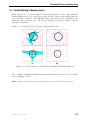
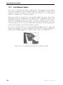
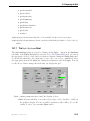
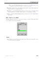
3.1.2
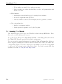
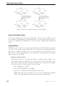
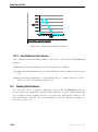
Menu Bar
The menu bar organizes the GUI menu hierarchy using a set of pull-down menus (see
Figure 3.1.2). Menu items are arranged in a logical order to correspond to the sequence
of actions that you perform in TGrid.
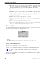
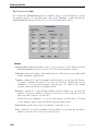
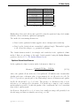
Figure 3.1.2: The TGrid Menu Bar
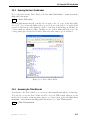
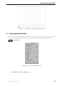
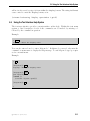
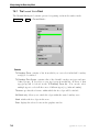
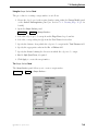
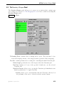
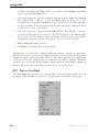
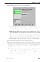
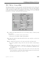
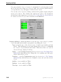
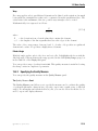
A pull-down menu contain items that perform commonly executed actions. Figure 3.1.3
shows the (UNIX) Report pull-down menu.
Using the Mouse
To select any item from the pull-down menu, do the following:
1. Click the pull-down menu using the left mouse button.
2. Move the pointer to the item you want to select and click it.
3. Release the left mouse button.
c ANSYS, Inc. April 15, 2008
3-3
Graphical User Interface
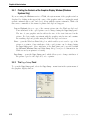
Figure 3.1.3: The Report Pull-down Menu
Using the Mnemonic (Windows Systems Only)
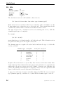
You can also select a pull-down menu item using the keyboard. Each pull-down menu
label or menu item contains one underlined character, known as the mnemonic.
1. Press the <Alt> key and the mnemonic character of the pull-down menu to display
a menu.
2. When the pull-down menu is displayed, type the mnemonic character associated
with an item to select that item. If at any time you want to cancel a menu selection
while the pull-down menu is displayed, press the <ESC> key.
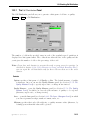
3.2
Dialog Boxes
A dialog box is a separate, temporary window that is displayed to perform the dialog.
The dialog boxes are used to perform simple input/output tasks, such as issuing warning
and error messages, or asking a question requiring a yes or no answer. When a dialog
box appears on your screen, you should take care of it before moving on to other tasks.
Different types of dialog boxes are described in the following sections.
3.2.1 Error Dialog Box
3-4
c ANSYS, Inc. April 15, 2008
3.2 Dialog Boxes
The Error dialog box is used to alert you of an error that has occurred. After reading the
error information, click OK to close the dialog box.
3.2.2 Information Dialog Box
The Information dialog box is used to report some information to you. After reading the
information, click OK to close the dialog box.
3.2.3 Warning Dialog Box
The Warning dialog box is used to alert you of a potential problem and ask you whether
or not you want to proceed with the current operation. Click OK to proceed with the
operation. Click Cancel to cancel the operation.
3.2.4 Working Dialog Box
The Working dialog box is displayed when TGrid is busy performing a task. When the
task is done, the dialog box will close automatically.
c ANSYS, Inc. April 15, 2008
3-5
Graphical User Interface
This is a special dialog box, because it requires no action by you. However, you can abort
the task that is being performed by clicking the Cancel button.
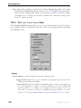
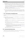
3.2.5 Question Dialog Box
The Question dialog box is used to ask you a question that requires an answer (Yes or
No). Click on the appropriate button to answer the question.
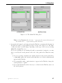
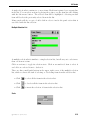
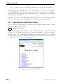
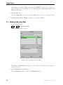
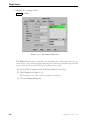
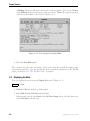
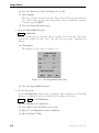
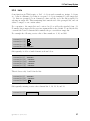
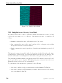
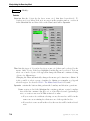
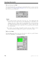
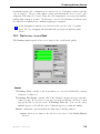
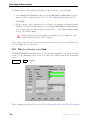
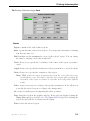
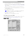
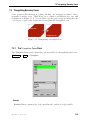
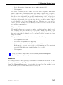
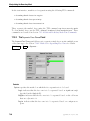
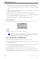
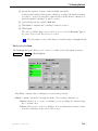
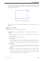
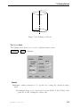
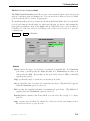
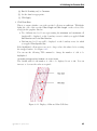
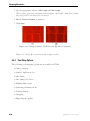
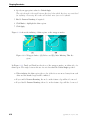
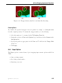
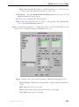
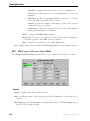
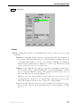
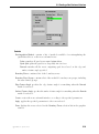
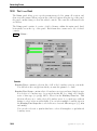
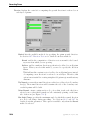
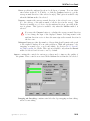
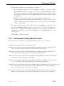
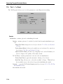
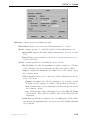
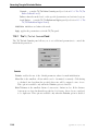
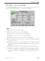
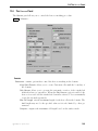
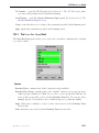
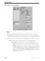
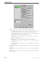
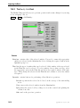
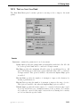
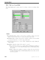
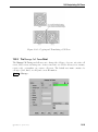
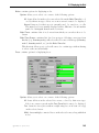
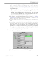
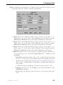
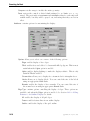
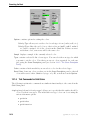
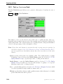
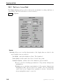
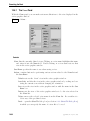
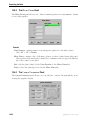
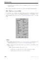
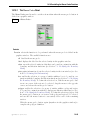
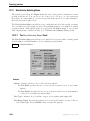
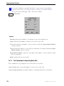
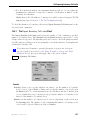
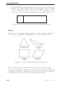
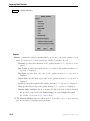
3.2.6 Select File Dialog Box
The Select File dialog box allows you to select a file (or multiple files) for reading or
writing. You can use it to look at your system directories and to select a file. The
appearance of the Select File dialog box will not always be the same.
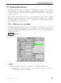
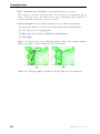
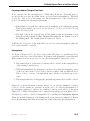
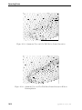
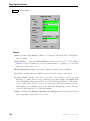
• When you select the File/Read/Mesh... or File/Read/Boundary Mesh... menu item
to read a mesh file, the Select File dialog box will look as shown in Figure 3.2.1(A).
• If you are writing a case file, the dialog box will look as shown in Figure 3.2.1(B).
• If you are reading or writing any other type of file, the dialog box will be similar to
that in Figure 3.2.1(B), except that the Write Binary Files and Write As Polyhedra
buttons will not appear.
To select files on UNIX systems, do the following:
1. Go to the appropriate directory. You can do this in two different ways:
• Enter the path to the desired directory in the Filter text entry box and press
the <RETURN> key or click the Filter button.
Note: Include the final “ / ” character in the pathname, before the optional
search pattern.
• Double-click a directory, and then a subdirectory, etc. in the Directories list
until you reach the directory you want. You can also click once on a directory
and then click Filter instead of double-clicking.
3-6
c ANSYS, Inc. April 15, 2008
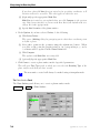
3.2 Dialog Boxes
Figure 3.2.1: The Select File Dialog Box
Note: In the Directories list, the dot “.” represents the current directory and
the double dots “..” represents the parent directory.
2. Specify the file name by selecting it from the Files list or entering the file name in
the File text entry box (if available) at the bottom of the dialog box. The name
of this text entry box will change depending on the type of file you are selecting
(Mesh File, Journal File, etc.).
If you are searching for an existing file with a non-standard extension, you may
have to modify the search pattern at the end of the path in the Filter text entry
box.
• If you are reading a mesh file, the default extension in the search path will be
*.{msh,MSH,cas}*, and only those files that have one of these extensions will
appear in the Files list.
• If you want files with a .grd extension to appear in the Files list, change the
search pattern to *.grd*.
• If you want all the files in the directory to be listed in the Files list, enter * as
the search pattern.
c ANSYS, Inc. April 15, 2008
3-7
Graphical User Interface
3. Read multiple boundary mesh or volume mesh files.
• If you are reading multiple boundary mesh or volume mesh files, the selected
file will be added to the list of Mesh File(s). You can then select another file,
which will also be added to this list.
• If you have put only the required files in the working directory and want to
read all of them, click the Select All button. All the files available in the
directory will be added to the list of Mesh File(s).
• If you accidentally select the wrong file, select it in the Mesh File(s) list and
click the Remove button to remove it from the list of files to be read. Repeat
until only the required files are in the Mesh File(s) list.
• You can also read multiple boundary mesh or volume mesh files using the
Append File(s) option. Open the Select File dialog box and read the first mesh
file in TGrid. Open the Select File dialog box again, enable the Append File(s)
check button and read the remaining mesh files one after the other.
i
The Append File(s) option will not be accessible while reading the first
mesh file. It will be accessible only after reading the first mesh file.
4. To write a mesh file, enter the file name in the Mesh File text entry box and click
OK.
!
The Write Binary Files check button is enabled by default. Binary files take
up less space and can be read and written by TGrid more quickly. The
binary files are written in double-precision.
You can disable the Write Binary Files option to write the file in text format. You
can read and edit the text file, but it will require more storage space than the
corresponding binary file.
You can also use the following TUI command to toggle the Write Binary Files option:
/file/file-format
5. To write a hexcore mesh, enable Write As Polyhedra check button in the Select File
panel to allow TGrid to handle polyhedral cells. Polyhedral cells are created when
hex and tet cells are merged with each other. Enabling this option allows TGrid to
export these cells instead of nonconfomal meshes.
i
This option is available only for hexcore meshes.
6. Click OK to read or write the specified file(s). Shortcuts for this step are as follows:
• If the file appears in the Files list and you are not reading a mesh, doubleclick on it instead of just selecting it. This will automatically activate the OK
button.
3-8
c ANSYS, Inc. April 15, 2008
3.3 Panels
• If you are reading a mesh, you will always have to click OK. Clicking or doubleclicking will just add the selected file to the Mesh File(s) list.
• If you entered the name of the file in the File text entry box, press the <RETURN>
key instead of clicking OK.
File selection on Windows systems can be done using the standard Windows Select File
dialog box. For further instructions, see documentation regarding your Windows system.
3.3
Panels
A panel is similar to a dialog box, but working with a panel is like filling out a form.
Panels are used to perform more complicated input tasks. Each panel is unique and
employs various types of input controls that make up the form. The various types of
controls you will see are described in the following sections.
3.3.1
Categories of Panels
After entering the data using the controls of a panel, you can either apply the changes you
have made, or abort the changes. Each panel falls into one of two behavioral categories,
depending on how it was designed (for applying or aborting the changes).
• Some panels are used in situations where you have to apply the changes and immediately close the panel.
This type of panel includes two push button controls:
OK applies any changes you have made to the panel and closes the panel.
Cancel ignores the changes you have made and closes the panel.
• Some panels are used in situations where you have to keep the panel displayed on
the screen after changes have been applied. This helps to quickly go back to that
panel and make more changes. Panels used for mesh generation and display often
fall into this category.
c ANSYS, Inc. April 15, 2008
3-9
Graphical User Interface
This type of panel includes two push button controls:
Apply applies any changes you have made to the panel, but does not close the
panel. The name of this button is often changed to something more descriptive
(for example, Sort for the sorting panels).
Close closes the panel.
All panels include the Help push button used to access on-line help. It displays information about the controls in the panel. The help information will appear in the web
browser.
3.3.2
Controls of a Panel
Different types of controls in the panels are described in the following sections.
Tab
Tabs in the panel are used to mark the different sections into which the panel is divided.
The panel may be divided into different sections to reduce the amount of screen space it
occupies. Click on a tab to access that particular section of the panel.
Button
3-10
c ANSYS, Inc. April 15, 2008
3.3 Panels
A button is used to perform a function indicated by the button label. Click on the button
to perform the action associated with it.
Check Box
A check box, also referred to as check button is a dialog element that is used to select or
deselect an option.
It is located on forms and can appear alone or in groups of two or more and is used to
enable/disable an item or action indicated by the label of the check box. Click the left
mouse button on the check box to toggle the state.
Radio Buttons
Radio buttons are a set of check buttons that allow only one to be set in the on position
at a time. When you click the left mouse button on a radio button, it will turn on, and
all others will be turned off.
Text Entry
A text entry lets you type the text input. It will often have a label associated with it to
indicate what the entry is for.
Integer Number Entry
c ANSYS, Inc. April 15, 2008
3-11
Graphical User Interface
An integer number entry is similar to a text entry except it allows only integer numbers
to be entered (e.g., 10, -10, 50000, and 5e4). The integer number entry also has arrow
buttons that allow you to increase or decrease its value.
Click on the up (or down) arrow button to increase (or decrease) the value by one. You
can increase the size of the increment by holding down a keyboard key while clicking the
arrow button. The keys used are:
Key
Factor of Increase
Shift 10
Ctrl
100
Real Number Entry
A real number entry is similar to a text entry except it allows only real numbers to be
entered (e.g., 10, -10.538, 50000.45, and 5.e-4). In most cases, the label will show the
units associated with the real number entry.
Single-Selection List
3-12
c ANSYS, Inc. April 15, 2008
3.3 Panels
A single-selection list contains two or more items. Each item is printed on a separate line
in the list. You can select an item by placing the pointer over the item line and clicking
with the left mouse button. The selected item will be highlighted. Selecting another
item will deselect the previously selected item in the list.
Many panels will also accept a double-click in order to invoke the panel action that is
associated with the list selection.
Multiple-Selection List
A multiple-selection list is similar to a single-selection list, but allows you to select more
than one item at a time.
Click on an item, to toggle its selection state. Click on an unselected item to select it
and click on a selected item to deselect it.
There are three small push buttons in the upper right corner of the multiple selection
list, which accelerate the task of selecting or deselecting items from the selection list.
• Click
to select all the items in the selection list.
• Click
to deselect all the items in the selection list.
• Click
to invert the selection of items in the selection list.
Scale
c ANSYS, Inc. April 15, 2008
3-13
Graphical User Interface
The scale is used to select a value from a predefined range by moving a slider. The
number shows the current value. To change the value, do the following:
1. Place the pointer over the slider.
2. Press and hold down the left mouse button.
3. Move the pointer along the slider bar to change the value.
4. Release the left mouse button.
OR
1. Place the pointer over the slider and click the left mouse button.
2. Using the arrow keys on the keyboard, move the slider bar left or right to change
the value.
Drop-Down List
A drop-down list is a hidden single-selection list that shows only the current selection to
save space.
To change the selection, do the following:
1. Click on the arrow button to display the list.
2. Place the pointer over the new list item.
3. Click the left mouse button on the item to make the selection and close the list.
To abort the selection operation while the list is displayed, move the pointer anywhere
outside the list and click the left mouse button.
3-14
c ANSYS, Inc. April 15, 2008
3.4 Graphics Display Windows
3.4
Graphics Display Windows
Graphics display windows (e.g., Figure 3.4.1) are separate windows that display the
graphical output of the program.
• Use the Display Options panel to change the attributes of the graphics display or to
open another display window.
• Use the Mouse Buttons panel to set the action taken when a mouse button is pressed
in the display window.
Figure 3.4.1: Graphics Display Window
• To cancel a display operation, press <Control-C> while the data is being processed
in preparation for graphical display.
i
You cannot cancel the operation after the program begins to draw in the
graphics window.
For Windows systems, there are special features for printing the contents of the graphics
window directly. These features are not available on UNIX systems.
c ANSYS, Inc. April 15, 2008
3-15
Graphical User Interface
3.4.1
Printing the Contents of the Graphics Display Window (Windows
Systems Only)
If you are using the Windows version of TGrid, the system menu of the graphics window
displayed by clicking in the upper-left corner of the graphics window, contains the usual
system commands (move, size, and close). Along with the system commands, TGrid adds
three more commands to the menu for printer and clipboard support.
Copy to Clipboard places a copy of the current picture into the Windows clipboard.
Some attributes of the copied picture can be changed using the Page Setup panel.
The size of your graphics window affects the size of the text fonts used in the
picture. For best results, experiment with the graphics window size and examine
the resulting clipboard picture using the Windows clipboard viewer.
Print... opens the Windows Print dialog box, which enables you to send a copy of the
picture to a printer. Some attributes of the copied picture can be changed using
the Page Setup panel. More attributes of the final print can be specified within
the Microsoft Windows Print and Print Setup dialog boxes (see documentation for
Windows and your printer for details).
Page Setup... opens the Page Setup panel, which allows you to change attributes of
the picture copied to the clipboard, or to a printer.
3.4.2
The Page Setup Panel
To open the Page Setup panel, select the Page Setup... menu item in the system menu of
the graphics display window.
3-16
c ANSYS, Inc. April 15, 2008
3.4 Graphics Display Windows
Controls
Color allows you to specify a color or non-color picture.
Color selects a color picture.
Gray Scale selects a gray-scale picture.
Monochrome selects a black-and-white picture.
Color Quality allows you to specify the color mode used for the picture.
True Color creates a picture defined by RGB values. This assumes that your
printer (or display) has at least 65536 colors, or unlimited colors.
Mapped Color creates a picture that uses a colormap. This is the right choice
for devices that have 256 colors.
Dithered Color creates a dithered picture that uses 20 colors or less.
Clipboard Formats allows you to choose the desired format copied to the clipboard.
The size of your graphics window can affect the size of the clipboard picture. For
best results, experiment with the graphics window size and examine the resulting
clipboard picture using the Windows clipboard viewer.
Bitmap is a bitmap copy of the graphics window.
DIB Bitmap is a device-independent bitmap copy of the graphics window.
Metafile is a Windows Metafile.
Enhanced Metafile is a Windows Enhanced Metafile.
Picture Format allows you to specify a raster or a vector picture.
Vector creates a vector picture. This format will have a higher resolution when
printed, but some large 3D pictures may take a long time to print.
Raster creates a raster picture. This format will have a lower resolution when
printed, but large 3D pictures may take much less time to print.
Printer Scale % controls the amount of the page that the printed picture will cover.
Decreasing the scaling will effectively increase the margin between the picture and
the edge of the paper.
Options contains options that control other attributes of the picture.
Landscape Orientation (Printer) specifies the orientation of the picture. If selected, the picture is made in landscape mode. Otherwise, it is made in portrait mode. This option is applicable only when printing.
Reverse Foreground/Background specifies that the foreground and background
colors of the picture will be swapped. This feature allows you to make a copy
of the picture with a white background and a black foreground, while the
graphics window is displayed with a black background and white foreground
respectively.
c ANSYS, Inc. April 15, 2008
3-17
Graphical User Interface
3.5
Customizing the GUI (UNIX Systems)
On UNIX systems, you can customize the GUI by changing the attributes such as text
color, background color, and text fonts. The program will try to provide default text fonts
that are satisfactory for the display size of your platform. In some cases, customization
may be necessary if the default text fonts make the GUI too small or too large on your
display, or if the default colors are undesirable.
The GUI in TGrid is based on the X Window System Toolkit and OSF/Motif. The attributes of the GUI are represented by X Window “resources”. If you are unfamiliar
with the X Window System Resource Database, please refer to any documentation you
may have that describes how to use the X Window System or OSF/Motif applications.
The default X Window resource values for a medium resolution display are as follows:
!
! General resources
!
Fluent*geometry:
+0-0
Fluent*fontList:
*-helvetica-bold-r-normal--12-*
Fluent*MenuBar*fontList:
*-helvetica-bold-r-normal--12-*
Fluent*XmText*fontList:
*-fixed-medium-r-normal--13-*
Fluent*XmTextField*fontList:
*-fixed-medium-r-normal--13-*
Fluent*foreground:
black
Fluent*background:
gray75
Fluent*activeForeground:
black
Fluent*activeBackground:
gray85
Fluent*disabledTextColor:
gray55
Fluent*XmToggleButton.selectColor:
green
Fluent*XmToggleButtonGadget.selectColor: green
Fluent*XmText.translations:\
#override<Key>Delete: delete-previous-character()
Fluent*XmTextField.translations:\
#override<Key>Delete: delete-previous-character()
!
! Console resources
!
Fluent*ConsoleText.rows:
24
Fluent*ConsoleText.columns:
80
Fluent*ConsoleText.background: linen
!
! Help Viewer resources
!
Fluent*Hyper.foreground:
3-18
black
c ANSYS, Inc. April 15, 2008
3.6 Using the GUI Help System
Fluent*Hyper.background:
linen
Fluent*Hyper.hyperColor:
SlateBlue3
Fluent*Hyper*normalFont:\
*-new century schoolbook-medium-r-normal--12-*
Fluent*Hyper*hyperFont:\
*-new century schoolbook-bold-r-normal--12-*
Fluent*Hyper*texLargeFont:\
*-new century schoolbook-bold-r-normal--14-*
Fluent*Hyper*texBoldFont:\
*-new century schoolbook-bold-r-normal--12-*
Fluent*Hyper*texFixedFont:\
*-courier-bold-r-normal--12-*
Fluent*Hyper*texItalicFont:\
*-new century schoolbook-medium-i-normal--12-*
Fluent*Hyper*texMathFont:\
*-symbol-medium-r-normal--14-*
Fluent*Hyper*texSansFont:\
*-helvetica-bold-r-normal--12-*
To customize one or more of the resources for a particular user, place appropriate resource
specification lines in that user’s file $HOME/.Xdefaults or whatever resource file is loaded
by the X Window System on the user’s platform.
To customize one or more of the resources for several users at a site, place the resource
specification lines in an application defaults resource file called Fluent. This file should
then be installed in a directory such as /usr/lib/X11/app-defaults, or on SUN workstations, the directory may be /usr/openwin/lib/app-defaults. See documentation
regarding your platform for more information.
3.6
Using the GUI Help System
TGrid includes an intergrated HTML-based on-line help system that provides an easy
access to the documentation. Using the graphical user interface, you can access the
entire User’s Guide and other documentation. The User’s Guide and other manuals are
displayed in your web browser, and you can use the hypertext links and the browser’s
search and navigation tools to find the information you need.
There are many ways to access the information contained in the on-line help.
• You can get reference information from within a panel (on UNIX machines).
• You can also request context-sensitive help for a particular menu item or panel.
• You can go to the User’s Guide contents page or index, and use the hypertext links
there to find the information you are looking for.
c ANSYS, Inc. April 15, 2008
3-19
Graphical User Interface
• You can also access the other TGrid documentation (e.g., the Tutorial Guide).
TGrid’s help system is HTML-based, so you need to have access to a web browser. Install the HTML files from the documentation CD-ROM. See the separate installation
instructions for your platform type for information about installing the files from the
documentation CD-ROM
This section focuses on the Help menu in TGrid and how you can use it (and the Help
button in each panel) to access the HTML-based on-line help from within TGrid.
3.6.1
Opening the User’s Guide Table of Contents
To see a list of the chapters in the User’s Guide, select the User’s Guide Contents... menu
item in the Help pull-down menu.
Help −→User’s Guide Contents...
Selecting this item will open the web browser to the contents page of the User’s Guide
(Figure 3.6.1). Each chapter in the list is a hypertext link that you can click to view that
chapter. There is also an Expanded Contents link, which will display a list of contents
including all section titles in addition to the chapter titles. Each of these is a link to the
corresponding chapter or section of the manual.
Figure 3.6.1: User’s Guide Contents
3-20
c ANSYS, Inc. April 15, 2008
3.6 Using the GUI Help System
3.6.2
Opening the User’s Guide Index
To see the index for the User’s Guide, select the User’s Guide Index... menu item in the
Help pull-down menu.
Help −→User’s Guide Index...
Selecting this menu item will open the web browser to the “A” page of the index (Figure 3.6.2). You can use the links at the top and bottom of the page to accessthe index
pages for other letters of the alphabet. Next to each entry in the index you will find one
or more numbers, which are links. Clicking on one of these links will bring you to the
corresponding place in the User’s Guide where the index entry topic is discussed.
Figure 3.6.2: User’s Guide Index
3.6.3 Accessing the Other Manuals
In addition to the User’s Guide, you can access other manuals through the on-line help.
You can also access the User’s Guide in Adobe Acrobat PDF format which is recommended if you want to print an entire chapter or a long section. Select the More Documentation... menu item in the Help pull-down menu to see other TGrid manuals.
Help −→More Documentation...
c ANSYS, Inc. April 15, 2008
3-21
Graphical User Interface
When you select this item, the web browser will open to the TGrid documentation home
page.
3.6.4 Using Help
You can obtain information about using on-line help by selecting the Using Help... menu
item in the Help pull-down menu.
Help −→Using Help...
When you select this item, the web browser will open to the beginning of this section.
3.6.5
Accessing the User Service Center Web Site
You can access the Fluent Users Service Center (USC) web site by selecting the User
Services Center... menu item in the Help pull-down menu.
Help −→User Services Center...
TGrid will direct your web browser to the USC web address.
Note: To link to the USC on UNIX platforms, first install the contents of the TGrid
Documentation CD, which contains the files necessary to launch the browser so
that you can automatically view the appropriate web pages.
3.6.6
Accessing the Online Technical Support Web Site
You can access the Online Technical Support web site by selecting the Online Technical
Support... menu item in the Help pull-down menu.
Help −→Online Technical Support...
TGrid will direct your web browser to the appropriate web address.
3.6.7
Obtaining a Listing of Other TGrid License Users
You can obtain a listing of current TGrid users when you select the License Usage... menu
item in the Help pull-down menu.
Help −→License Usage...
TGrid will display a list the current users of the TGrid license feature in the console
window.
3-22
c ANSYS, Inc. April 15, 2008
Chapter 4.
Sample Session
This chapter describes a sample session to illustrate the basic procedure for examining
and creating the mesh in TGrid.
This sample session consists of the following steps:
• Section 4.1: Preparation
• Section 4.2: Reading the Boundary Mesh
• Section 4.3: Examining the Boundary Mesh
• Section 4.4: Generating the Interior Mesh
• Section 4.5: Displaying the Mesh
• Section 4.6: Reporting the Mesh Statistics
• Section 4.7: Checking the Mesh
• Section 4.8: Saving the Mesh and Exiting TGrid
In this session, you will generate a triangular volume mesh for a simple wedge-shaped
geometry. The boundary mesh file is provided with TGrid on the CD.
4.1
Preparation
1. Copy wedge.zip from the TGrid documentation CD to your working directory.
• For UNIX systems, locate the file by inserting the CD into your CD-ROM
drive and going to the following directory:
cdrom/tgrid5.0/help/tutfiles/
Replace cdrom by the name of your CD-ROM drive.
• For Windows systems, locate the file by inserting the CD into your CD-ROM
drive and going to the following directory:
cdrom:\tgrid5.0\help\tutfiles\
Replace cdrom by the name of your CD-ROM drive (e.g., E).
c ANSYS, Inc. April 15, 2008
4-1
Sample Session
Alternatively, download wedge.zip from the FLUENT User Services Center to
your working directory. This file can be found from the Documentation link on the
TGrid product page.
2. Unzip wedge.zip.
The file, wedge.msh can be found in the wedge folder created on unzipping the file.
3. Start the 2D version of TGrid (see Section 2.2: Starting TGrid).
4.2
Reading the Boundary Mesh
1. Read in the mesh file.
File −→ Read −→Boundary Mesh...
The Select File dialog will open.
Figure 4.2.1: Reading the Mesh File
The Filter and Directories that appear in the dialog box depend on the location of
working directory.
2. Select wedge.msh in the Files list.
The file wedge.msh will be added to the Mesh File(s) list.
4-2
c ANSYS, Inc. April 15, 2008
4.3 Examining the Boundary Mesh
3. Click OK.
TGrid will read the mesh file and it’s console shows the progress as the file is read.
4.3 Examining the Boundary Mesh
After reading the mesh file, you can check the boundary mesh for topological problems
such as free and multi-connected nodes and faces. All these operations can be performed
in the Merge Boundary Nodes panel. You can display the grid using the Display Grid panel.
Boundary −→Merge Nodes...
Figure 4.3.1: The Merge Boundary Nodes Panel
1. Click Count Free Nodes to see if any free nodes exist.
TGrid reports (in the Message field) that none were found. You can click Merge to
merge the free nodes, if any exist.
2. Click Count Unused Nodes to see if any unused nodes exist.
You can click Delete Unused Nodes to delete unused nodes, if any exist.
3. Close the Merge Boundary Nodes panel.
For a 3D surface mesh, you can use the Boundary Improve panel (also opened from
the Boundary menu) to check the boundary mesh quality and make improvements.
c ANSYS, Inc. April 15, 2008
4-3
Sample Session
4. Display the boundary mesh.
Display −→Grid...
Figure 4.3.2: The Display Grid Panel
The Display Grid panel has capabilities for displaying free, multi-connected, and unmeshed faces. It is useful to display unmeshed faces when the initial mesh generation
process fails and you want to locate the problem areas easily.
(a) Select all the boundary zones in the Face Zones selection list.
(b) Click Display (see Figure 4.3.3).
The boundaries are color coded according to their type.
(c) Close the Display Grid panel.
4-4
c ANSYS, Inc. April 15, 2008
4.4 Generating the Interior Mesh
Figure 4.3.3: Display of Wedge Boundary Faces
4.4
Generating the Interior Mesh
When you are satisfied with the boundary mesh, generate the interior mesh. For most
cases, the automatic mesh generation procedure will create an good-quality mesh.
Mesh −→Auto Mesh...
Figure 4.4.1: The Auto Mesh Panel
1. Click Mesh in the Auto Mesh panel.
c ANSYS, Inc. April 15, 2008
4-5
Sample Session
A Working dialog box will appear during the mesh generation. You can click Cancel
in the Working dialog box to stop the mesh generation. TGrid will report the progress
of the mesh generation in the console (Figure 4.4.2).
Figure 4.4.2: Text Output from Auto Mesh
2. Close the Auto Mesh panel.
This example describes the generation of the mesh using the default triangular mesh
generation parameters. You can modify the mesh generation parameters in the Tri/Tet
panel (see Section 11.5: The Tri/Tet Panel), if required.
4.5
Displaying the Mesh
You can display the mesh using the Display Grid panel (Figure 4.5.1).
Display −→Grid...
1. Click the Cells tab at the top of the panel.
2. Select fluid-8 in the Cell Zones selection list.
Alternatively, you can select fluid in the Cell Zone Groups list to select the fluid zone
in the Cell Zones selection list.
4-6
c ANSYS, Inc. April 15, 2008
4.5 Displaying the Mesh
Figure 4.5.1: The Display Grid Panel—Cells Tab
3. Enable All in the Options group box.
4. Click Display (see Figure 4.5.2).
Figure 4.5.2: Grid Display
5. Close the Display Grid panel.
The Cell Zones list has a dead zone. When TGrid initializes the mesh, it automatically
makes the cell zone with the largest volume (or the cell zone that contains a boundary
zone with type pressure-outlet) the active fluid zone.
c ANSYS, Inc. April 15, 2008
4-7
Sample Session
TGrid treats the rest of the cell zones (non-fluid zones) as dead zones. In this case, there
is a dead zone for the region inside the wedge (see Figure 4.5.3). Since the cells in the
dead zone are not in the computational domain, they can be ignored.
When you read the mesh into the solver, the dead cell zones will be ignored. If you
have a large mesh with many cells in a dead zone, you can delete the dead zones using
the Manage Cell Zones panel. This reduces the memory requirements. You can zoom
in on the wedge using the middle mouse button to create a zoom box around it (see
Section 14.9: Controlling the Mouse Buttons for details). The resulting display is shown
in Figure 4.5.3.
Figure 4.5.3: Grid—Zoomed View
4.6
Reporting the Mesh Statistics
It is important to examine the grid statistics in the Report menu. Looking at tetrahedral
cells does not provide much useful information about the mesh. Hence, you need to rely
primarily on grid statistics.
1. Open the Report Boundary Cell Limits panel.
Report −→Boundary Cell Limits...
(a) Click Compute.
The maximum cell skewness of cells having 1 boundary face is 0.47. A skewness
of zero indicates an equilateral cell. You can click the Quality Measure... button
to open the Quality Measure panel (see Section 15.5.2: The Quality Measure
Panel) where you can report additional measures of quality (aspect ratio and
4-8
c ANSYS, Inc. April 15, 2008
4.6 Reporting the Mesh Statistics
Figure 4.6.1: The Report Boundary Cell Limits Panel
change in size) by selecting them. The default measure of skewness is sufficient
for analyzing the quality of triangular and tetrahedral cells.
(b) Close the Report Boundary Cell Limits panel.
2. Open the Report Cell Limits panel.
Report −→Cell Limits...
Figure 4.6.2: The Report Cell Limits Panel
You can use this panel to determine the best (minimum), worst (maximum), and
average cell quality (skewness, by default).
(a) Select Quality in the Options list.
c ANSYS, Inc. April 15, 2008
4-9
Sample Session
(b) Select the fluid-7 zone in the Cell Zones selection list.
(c) Click Compute.
The worst cell has a skewness of 0.488. The average skewness is approximately
0.12. These values are typical for 2D problems and are suitable for obtaining
a solution using FLUENT.
(d) Close the Report Cell Limits panel.
3. Open the Report Mesh Size panel.
Report −→Mesh Size...
You can use this panel to check the number of nodes, faces, and cells. This panel
separates the number of nodes, faces, and cells into two groups—boundary and
interior.
(a) Click Update.
The number of cells is 664 (see Figure 4.6.3).
Figure 4.6.3: The Report Mesh Size Panel
(b) Close the Report Mesh Size panel.
4. Plot the histogram.
Use the Cell Distribution panel to plot a histogram of the distribution of cell quality
(skewness, by default) to get an overall feel of the quality of the mesh.
Display −→ Plot −→Cell Distribution...
(a) Select Quality in the Options list.
(b) Select fluid-7 in the Cell Zones selection list.
(c) Enter 0.5 for Maximum and 50 for Partitions.
(d) Enable Percent of Total.
4-10
c ANSYS, Inc. April 15, 2008
4.6 Reporting the Mesh Statistics
(e) Click Plot.
TGrid will plot the histogram shown in Figure 4.6.4.
Figure 4.6.4: Histogram of Cell Quality (Skewness)
(f) Close the Cell Distribution panel.
c ANSYS, Inc. April 15, 2008
4-11
Sample Session
4.7
Checking the Mesh
Before saving the mesh file, check it to make sure it has no negative cell volumes or
left-handed faces. See Section 13.11: Checking the Mesh for details.
Mesh −→Check
Domain extents.
x-coordinate: min = -1.000000e+01, max = 1.000000e+01.
y-coordinate: min = -1.000000e+01, max = 1.000000e+01.
Volume statistics.
minimum volume: 1.246947e-03.
maximum volume: 2.172626e+00.
total volume: 3.999559e+02.
Face area statistics.
minimum face area: 1.022265e-02.
maximum face area: 2.254692e+00.
average face area: 9.797752e-01.
Checking number of nodes per cell.
Checking number of faces per cell.
Checking cell faces.
Checking face handedness.
Checking periodic face pairs.
Checking face children.
Checking face zone boundary conditions.
Checking for invalid node coordinates.
Done.
The printed results of the check do not show any problem, hence, the mesh is valid for
use in FLUENT.
4.8
Saving the Mesh and Exiting TGrid
File −→ Write −→Mesh...
1. Enter the file name (wedge-final.msh) in the Mesh File field.
2. Click OK to write the file.
The default file name is the same as the input file name.
4-12
c ANSYS, Inc. April 15, 2008
4.8 Saving the Mesh and Exiting TGrid
Figure 4.8.1: Writing the Mesh File
3. End the TGrid session by selecting Exit in the File menu.
File −→Exit
Alternatively, you can type /exit in the TGrid console.
c ANSYS, Inc. April 15, 2008
4-13
Sample Session
4-14
c ANSYS, Inc. April 15, 2008
Chapter 5.
Text User Interface
TGrid user interface also consists of a textual command line reference. The text user
interface (TUI) is written in a dialect of Lisp called Scheme. Users familiar with Scheme
will be able to use the interpretive capabilities of the interface to create customized
commands. The TUI is described in the following sections:
• Section 5.1: Text Menu System
• Section 5.2: Text Prompt System
• Section 5.3: Interrupts
• Section 5.4: System Commands
• Section 5.5: Text Menu Input from Character Strings
• Section 5.6: Using the Text Interface Help System
5.1
Text Menu System
The text menu system provides a hierarchical interface to the program’s underlying
procedural interface.
• You can easily manipulate its operation with standard text-based tools: input can
be saved in files, modified with text editors, and read back in to be executed,
because it is text based.
• The text menu system is tightly integrated with the Scheme extension language,
so it can easily be programmed to provide sophisticated control and customized
functionality.
The menu system structure is similar to the directory tree structure of UNIX operating
systems. When you first start TGrid, you are in the “root” menu and the menu prompt
is simply a caret:
>
c ANSYS, Inc. April 15, 2008
5-1
Text User Interface
To generate a listing of the submenus and commands in the current menu, press <RETURN>.
>
file/
boundary/
mesh/
display/
report/
exit
By convention, submenu names end with a / to differentiate them from menu commands.
To execute a command, type its name (or an abbreviation). Similarly, to move down
into a submenu, enter its name or an abbreviation. When you move into the submenu,
the prompt will change to reflect the current menu name.
> display
/display> set
/display/set>
To move back to the previously occupied menu, type q or quit at the prompt.
/display/set> q
/display>
You can move directly to a menu by giving its full pathname.
/display> /file
/display//file>
In the above example, control was passed from /display to /file without stopping in
the root menu. Therefore, when you quit from the /file menu, control will be passed
directly back to /display.
/display//file> q
/display>
If you execute a command without stopping in any of the menus along the way, control
will again be returned to the menu from which you invoked the command.
5-2
c ANSYS, Inc. April 15, 2008
5.1 Text Menu System
/display> /file start-journal jrnl
Input journal opened on file "jrnl".
/display>
The text menu system provides on-line help for menu commands. The text menu on-line
help system is described in Section 5.6: Using the Text Interface Help System.
5.1.1
Command Abbreviation
To select a menu command, you need not type the entire name; you can type an abbreviation that matches the command.
• A command name consists of “phrases” separated by hyphens.
• A command is matched by matching an initial sequence of its phrases.
• Matching of hyphens is optional.
• A phrase is matched by matching an initial sequence of its characters.
• A character is matched by typing that character.
The rules for “matching” a command are:
• If an abbreviation matches more than one command, then the command with the
greatest number of matched phrases is chosen.
• If more than one command has the same number of matched phrases, then the first
command to appear in the menu is chosen.
For example, each of the following will match the given command set-ambientcolor: set-ambient-color, s-a-c, sac, and sa.
• When abbreviating commands, sometimes your abbreviation will match more than
one command. In such cases, the first command is selected.
• Occasionally, there is an anomaly such as lint not matching lighting-interpolation
because the li gets absorbed in lights-on? and then the nt doesn’t match
interpolation.
This can be resolved by choosing a different abbreviation, such as liin, or l-int.
c ANSYS, Inc. April 15, 2008
5-3
Text User Interface
5.1.2 Scheme Evaluation
If you enter an open parenthesis ”(” at the menu prompt, then that parenthesis and all
characters up to and including the matching closing parenthesis are passed to Scheme to
be evaluated. The result of evaluating the expression is then displayed.
> (define a 1)
a
> (+ a 2 3 4)
10
5.1.3
Aliases
Command aliases can be defined within the menu system. As with the UNIX csh shell,
aliases take precedence over command execution. The following aliases are predefined in
Cortex (error, pwd, chdir, ls, ., and alias):
error displays the Scheme object that was the “irritant” in the most recent Scheme error
interrupt.
pwd prints the working directory in which all file operations will take place.
chdir changes the working directory.
ls lists the files in the working directory.
alias displays the list of symbols currently aliased.
5.2
Text Prompt System
Commands require various arguments, including numbers, filenames, yes/no responses,
character strings, and lists. A uniform interface to this input is provided by the text
prompt system. A prompt consists of a prompt string, followed by an optional units
string enclosed in parentheses, followed by a default value enclosed in square brackets
filled grids? [no]
<RETURN>
shrink-factor [0.1]
line-weight [1]
title [""]
5-4
<RETURN>
<RETURN>
<RETURN>
c ANSYS, Inc. April 15, 2008
5.2 Text Prompt System
• The default value for a prompt is accepted by typing a <RETURN> or a comma (,).
A comma is not a separator. It is a separate token that indicates a default value.
The sequence “1,2” results in three values
– the number 1 for the first prompt.
– the default value for the second prompt.
– the number 2 for the third prompt.
• A short help message can be displayed at any prompt by entering a ?. (See Section 5.6: Using the Text Interface Help System.)
• To abort a prompt sequence, press <Control-C>.
5.2.1
Numbers
The most common prompt type is a number. Numbers can be either integers or real
numbers. Valid numbers are, for example, 16, -2.4, .9e5, and +1e-5.
• Integers can also be specified in binary, octal, and hexadecimal form.
• The decimal integer 31 can be entered as 31, #b11111, #o37, or #x1f.
• In Scheme, integers are a subset of reals, so you do not need a decimal point to
indicate that a number is real; 2 is just as much a real as 2.0.
• If you enter a real number at an integer prompt, any fractional part will be truncated. That is, 1.9 will become 1.
5.2.2
Booleans
Some prompts require a yes-or-no response. A yes/no prompt will accept either yes or
y for a positive response, or no or n for a negative response. These prompts are used
for confirming potentially dangerous actions such as overwriting an existing file, exiting
without saving case, data, mesh, etc. Some prompts require actual Scheme boolean values
(true or false). These are entered with the Scheme symbols for true #t and false #f.
5.2.3
Strings
Character strings are entered in double quotes, as in "red". Plot titles and plot legend
titles are examples of character strings. Character strings can include any characters,
including blank spaces and punctuation.
c ANSYS, Inc. April 15, 2008
5-5
Text User Interface
5.2.4
Symbols
Symbols are entered without quotes. Zone names, surface names, and material names are
examples of symbols. Symbols must start with an alphabetical character (i.e., a letter),
and cannot include any blank spaces or commas.
You can use wild cards (*) to specify zone names when using the TUI. Some examples
are:
• /display/boundary-grid * allows you to display all the boundary zones in the
mesh.
• /boundary/delete-island-faces wrap* allows you to delete island faces on all
wrapper zones prefixed by wrap.
If you use a wild card for an operation that requires a single zone as input, you will
be prompted to specify a single zone from the list of those that match the expression
specified.
> /boundary/manage/name wall*
wall-1
wall-4
wall-2
wall-5
<RETURN>
wall-3
wall-6
Zone Name [ ]
5.2.5
Filenames
Filenames are actually character strings. For convenience, filename prompts do not
require the string to be surrounded with double quotes. If, for some exceptional reason,
a filename contains an embedded space character, then the name must be surrounded
with double quotes.
One consequence of this convenience is that filename prompts do not evaluate the response. For example, the following sequence will end up writing a hardcopy file with the
name fn, not valve.ps.
> (define fn "valve.ps")
fn
> hc fn
Since the filename prompt did not evaluate the response, fn did not get a chance to
evaluate "valve.ps" as it would for most other prompts.
5-6
c ANSYS, Inc. April 15, 2008
5.2 Text Prompt System
5.2.6
Lists
Some functions in TGrid require a “list” of objects such as numbers, strings, booleans,
etc. A list is a Scheme object that is a sequence of objects terminated by the empty list,
’(). Lists are prompted for an element at a time, and the end of the list is signaled by
entering an empty list. This terminating list forms the tail of the prompted list, and can
either be empty or can contain values.
For convenience, the empty list can be entered as () as well as the standard form ’().
Normally, list prompts save the previous argument list as the default. To modify the list,
overwrite the desired elements and terminate the process with an empty list.
For example the following creates a list of three numbers: 1, 10, and 100.
element(1)
element(2)
element(3)
element(4)
[()]
[()]
[()]
[()]
1
10
100
<RETURN>
Subsequently, it adds a fourth element as shown below:
element(1)
element(2)
element(3)
element(4)
element(5)
[1] <RETURN>
[10] <RETURN>
[100] <RETURN>
[()] <RETURN>
[()] <RETURN>
Then it leaves only 1 and 10 in the list:
element(1) [1] <RETURN>
element(2) [10] <RETURN>
element(3) [100] ()
Subsequently entering creates a five element list: 1, 10, 11, 12, and 13.
element(1) [1] ,,’(11 12 13)
c ANSYS, Inc. April 15, 2008
5-7
Text User Interface
Finally, a single empty list removes all elements:
element(1) [1] ()
5.2.7
Evaluation
All responses to prompts (except filenames), are “evaluated” by the Scheme interpreter
before they are used. Therefore you can enter any valid Scheme expression as the response
to a prompt. For example, to enter a unit vector with one component equal to 1/3
(without using your calculator), do the following:
/foo> set-xy
x-component [1.0] (/ 1 3)
y-component [0.0] (sqrt (/ 8 9))
You can also first define a utility function to compute the second component of a unit
vector as follows:
> (define (unit-y x) (sqrt (- 1.0 (* x x))))
unit-y
/foo> set-xy
x-component [1.0] (/ 1 3)
y-component [0.0] (unit-y (/ 1 3))
5.2.8
Default Value Binding
The default value at any prompt is bound to the Scheme symbol “_” (underscore) so
that the default value can form part of a Scheme expression. For example, if you want
to decrease a default value by one-third, you could enter
shrink-factor [0.8] (/ _ 3)
5.3
Interrupts
The execution of the code can be halted using <Control-C>, at which time the present
operation stops at the next recoverable location.
5-8
c ANSYS, Inc. April 15, 2008
5.4 System Commands
5.4
System Commands
If you are running TGrid in a UNIX operating system, you can execute system commands
with the ! (bang) shell escape character. All characters following the ! up to the next
newline character will be executed in a subshell. Any further input related to these
system commands must be entered in the window in which you started the program, and
any screen output will also appear in that window.
If you start TGrid remotely, this input and output will be in the window in which you
started Cortex.
> !rm junk.*
> !vi script.rp
The ls and pwd aliases invoke the UNIX ls and pwd commands in the working directory.
The chdir alias changes the current working directory of the program. The !ls and
!pwd commands will execute the UNIX commands in the directory in which Cortex was
started. The screen output will appear in the window in which you started TGrid, unless
you started it remotely, in which case the output will appear in the window in which you
started Cortex.
Note: Commands !chdir or !cd executes in a subshell, so it will not change the working
directory either for TGrid or for Cortex, and it is therefore not useful.
Typing chdir with no arguments will move you to your home directory in the console.
Examples of system commands entered in the console are as follows:
> !pwd
> !ls valve.*
The screen output will appear in the window in which TGrid was started. If you start
the program remotely, it will appear in the window in which Cortex was started.
/home/cfd/run/valve
valve1.cas
valve1.msh
c ANSYS, Inc. April 15, 2008
valve2.cas
valve2.msh
5-9
Text User Interface
5.5
Text Menu Input from Character Strings
When writing a Scheme extension function for TGrid, it is convenient to be able to
include menu commands in the function. This can be done with ti-menu-load-string.
For example, to open graphics window 1, use:
(ti-menu-load-string "di ow 1")
A Scheme loop that will open windows 0 and 1 and display the front view of the grid in
window 0 and the back view in window 1 is given by
(for-each
(lambda (window view)
(ti-menu-load-string (format #f "di ow ~a gr view rv ~a"
window view)))
’(0 1)
’(front back))
This loop makes use of the format function to construct the string used by menu-load-string.
This simple loop can also be written without using menu commands, but you need to
know the Scheme functions that get executed by the menu commands to do it:
(for-each
(lambda (window view)
(cx-open-window window)
(draw-mesh)
(cx-restore-view view))
’(0 1) ’(front back))
String input can also provide an easy way to create aliases within TGrid. For example,
to create an alias that will display the grid, you can type the following:
(alias ’dg (lambda () (ti-menu-load-string "/di gr")))
Then any time you enter dg from anywhere in the menu hierarchy, the grid will be drawn
in the active window.
ti-menu-load-string evaluates the string argument in the top level menu. It ignores
any menu you may be in when you invoke ti-menu-loadstring. Therefore, the command
(ti-menu-load-string "open-window 1 gr")
5-10
; incorrect usage
c ANSYS, Inc. April 15, 2008
5.6 Using the Text Interface Help System
will not work even if you type it from within the display/ menu. The string itself must
cause control to enter the display/ menu, as in
(ti-menu-load-string "display open-window 1 grid")
5.6
Using the Text Interface Help System
The text user interface provides context-sensitive on-line help. Within the text menu
system, a brief description of each of the commands can be invoked by entering a ?
followed by the command in question.
Example:
> ?dis
display/: Enter the display menu.
You can also enter a lone ? to enter “help mode.” In this mode, you need only enter the
command or menu name to display the help message. To exit help mode type q or quit
as for a normal menu.
Example:
> ?
[help-mode]> di
display/: Enter the display menu.
[help-mode]> pwd
pwd: #[alias]
(LAMBDA ()
(cx-send ’(system "pwd")))
[help-mode]> q
>
c ANSYS, Inc. April 15, 2008
5-11
Text User Interface
Help can also be obtained when you are prompted for information by typing a ? at the
prompt.
Example:
> display/annotate
Annotation text [""] ?
Enter the text to annotate the plot with.
Annotation text [""]
5-12
c ANSYS, Inc. April 15, 2008
Chapter 6.
File Types
During a TGrid session you may need to read and write several kinds of files. You can read
mesh, journal, Scheme, and domain files and write mesh, journal, transcript, and domain
files. TGrid also allows you to save hardcopy files, save panel layouts, and write the
current Scheme images. These files and features are described in the following sections.
• Section 6.1: Mesh Files
• Section 6.2: Compressed Files
• Section 6.3: Reading Scheme Source Files
• Section 6.4: Journal Files
• Section 6.5: Transcript Files
• Section 6.6: Domain Files
• Section 6.7: Importing Files
• Section 6.8: Exporting Files
• Section 6.9: Saving Hardcopy Files
• Section 6.10: Saving the Panel Layout
• Section 6.11: The .tgrid File
• Section 6.12: Exiting TGrid
6.1
Mesh Files
A mesh file includes a list of the node coordinates, boundary faces, and (sometimes)
interior faces and cells. The boundary faces are grouped into zones with specified boundary condition identifiers. In addition to reading and writing TGrid mesh files, you can
also import mesh files from various CAD packages and write mesh files for FLUENT.
For information about the format of the CAD package files, see Appendix A: Importing
Boundary and Volume Meshes, and for details on the mesh file format for TGrid and
FLUENT, see Appendix B: Mesh File Format.
c ANSYS, Inc. April 15, 2008
6-1
File Types
i
If the mesh information is contained in two or more separate files generated
by one of these CAD packages, you can read them one by one using the
Append File(s) check button in the Select File panel. You can also read
them together and have TGrid assemble the complete mesh for you.
By default, TGrid saves the mesh files with the suffix .msh. You need not type the suffix
while saving the mesh file, it will be added automatically. For example, if you enter the
file name gumby, TGrid will write to the file gumby.msh.
When TGrid reads a mesh file, it first searches for a file with the exact name you typed.
If a file with that name is not found, it will search for a file with .msh appended to the
name.
6.1.1
Reading Boundary Mesh Files
To read a FLUENT boundary mesh (contained in a FLUENT mesh file created with
GAMBIT or a boundary mesh contained in a FLUENT case file) into TGrid, you can do
either of the following:
• Select the File/Read/Boundary Mesh... menu item to open the Select File panel and
select the boundary mesh file to be read.
• Use the file/read-boundary-mesh text command and specify the name of the
boundary mesh file to be read.
This is convenient if you want to read in a large volume mesh and recreate it by starting
from the boundary mesh.
Reading Multiple Boundary Mesh Files
If the boundary mesh is contained in two or more separate files, you can read them
in together and have TGrid assemble the complete boundary mesh. Alternatively, you
can use the file/read-multi-bound-mesh text command for reading multiple boundary
mesh files.
6.1.2
Reading TGrid Mesh Files
To read a TGrid mesh, you can use either of the following:
• Select the File/Read/Mesh... menu item to open the Select File panel and select the
TGrid mesh file to be read.
• Use the file/read-mesh text command and specify the name of the mesh file to
be read.
6-2
c ANSYS, Inc. April 15, 2008
6.1 Mesh Files
You can also use either of these commands to read a FLUENT mesh file created with
GAMBIT, or to read the mesh file contained in a FLUENT case file. To do the latter, you
can also use the text command file/read-case.
The commands discussed here are used to read a 2D mesh into the 2D version of TGrid,
or a 3D mesh into the 3D version of TGrid.
i
TGrid cannot read grids from solvers that have been adapted using hanging
nodes. To read one of these grids into TGrid, coarsen the mesh within the
solver until you have recovered the original unadapted grid.
Reading Multiple TGrid Files
If the mesh is contained in two or more separate files, you can read them together in
TGrid and assemble the complete mesh. For example, if you are creating a hybrid mesh
by reading in a triangular boundary mesh and a volume mesh consisting of hexahedral
cells, read both files at the same time using the File/Read/Mesh... menu item or the
file/read-multiple-mesh or file/read-multiple-case text commands.
You can also use the file/read-meshes-by-tmerge text command. This command uses
the tmerge utility.
Reading 2D Mesh Files in the 3D Version of TGrid
It is also possible to read 2D meshes from FLUENT into the 3D version of TGrid. To read
a 2D mesh into the 3D version of TGrid, use the File/Import/Fluent 2D Mesh... menu item
or the file/import/fluent-2d-mesh text command.
Reading 3D Mesh Files in the 2D Version of TGrid
It is also possible to read 3D meshes from FLUENT into the 2D version of TGrid. To read
a 3D mesh into the 2D version of TGrid, use the File/Import/Fluent 3D Mesh... menu item
or the file/import/fluent-3d-mesh text command.
6.1.3
Appending Mesh Files
You can also read multiple mesh files one by one instead of reading all of them at a time.
This process is called as appending the mesh files. To do so, read in the first mesh file
using the Select File panel. Reopen the panel and enable Append File(s) check button and
read the remaining files one by one. For details, see Section 3.2.6: Select File Dialog Box.
You can also append the files using the following TUI command:
• file/append-meshes-by-tmerge allows you to append the mesh files using tmerge.
There is no GUI item in TGrid for this TUI command.
c ANSYS, Inc. April 15, 2008
6-3
File Types
• file/append-mesh allows you to append the mesh files. This command is same as
that of the Append File(s) check button in the Select File dialog box.
The Append File(s) check button is not accessible while reading the first mesh file.
6.1.4
Writing Mesh Files
To write a mesh file in the format that can be read by FLUENT, do either of the following:
• Select the File/Write/Mesh... menu item to open the Select File panel and specify
the name of the mesh file to be written.
• Use the file/write-mesh text command and specify the name of the mesh file to
be written.
To write a case file in the format that can be read by FLUENT, do either of the following:
• Select the File/Write/Case... menu item.
• Use the file/write-case text command and specify the name of the mesh file to
write.
Selecting the File/Write/Mesh... and File/Write/Case... menu item will invoke the Select
File panel, where you will specify the name of the mesh (or case) file to be written. By
default, a binary file will be written when you write a mesh or case file. Binary files take
up less memory than text files and can be read and written by TGrid more quickly.
You can disable the Write Binary Files option in the Select File dialog to write the file in
text format. The text file can be edited, but it will require more storage space than the
corresponding binary file. You can also use the TUI command /file/file-format to
toggle the writing of binary files.
Since FLUENT has the same mesh file format as TGrid, you will be able to read this file
back into TGrid using the File/Read/Mesh... menu item (or the file/read-mesh text
command) if you should need to modify the mesh at a later time.
If you are writing a hexcore mesh, enable the Write As Polyhedracheck button in the Select
File panel. This allows TGrid to create polyhedral cells. Polyhedral cells are created when
‘hex’ and ‘tet’ cells are merged with each other. Enabling this option allows TGrid to
export these cells instead of non-conformal meshes.
!
6-4
Case files containing polyhydral cells cannot be read in TGrid.
c ANSYS, Inc. April 15, 2008
6.1 Mesh Files
6.1.5
Writing Boundary Mesh Files
TGrid allows you to write a mesh file comprising specific boundary zones. This is useful
for large cases where you may want to mesh different parts of the mesh separately and
then merge them together. This allows you to avoid frequent switching between domains
for such cases. You can write out selected boundaries to a mesh file and then create the
volume mesh for the part in a separate TGrid session. You can then read the saved mesh
into the previous TGrid session using the Append File(s) option and merge the part with
the rest of the mesh.
To write a mesh file comprising selected boundaries, do either of the following:
• Use the File/Write/Boundaries... menu item to invoke the Write Boundaries panel
(see Section 6.1.5: The Write Boundaries Panel) and specify the boundaries to be
written.
• Use the /file/write-boundaries text command and specify the name of the file
to be written and the boundaries to be written.
The Write Boundaries Panel
The Write Boundaries panel allows you to specify the boundaries to be written to a mesh
file.
Controls
Boundary Zones contains a list of the boundary zones available.
Boundary Zone Groups contains a list of the boundary zone groups and user-defined
groups available.
c ANSYS, Inc. April 15, 2008
6-5
File Types
6.2
Compressed Files
TGrid allows you to read and write compressed files. Use the Select File dialog box to
read or write the files that have been compressed using compress or gzip.
6.2.1
Reading Compressed Files
If you select a compressed file with a .Z extension, TGrid will automatically invoke zcat
to import the file. If you select a compressed file with a .gz extension, TGrid will invoke
gunzip to import the file. For example, if you select a file named flow.msh.gz, TGrid
will report the following message indicating that the result of the gunzip is imported
into TGrid via an operating system pipe.
Reading "| gunzip flow.msh.gz"...
You can also read a compressed file using the text interface by entering the file name.
First, TGrid attempts to open a file with the input name. If it cannot find a file with
that name, it attempts to locate files with default suffixes and extensions appended to
the name. For example, if you enter the name file-name, TGrid traverses the following
list until it finds an existing file:
• file-name
• file-name.gz
• file-name.Z
• file-name.suffix
• file-name.suffix.gz
• file-name.suffix.Z
where suffix is a common extension to the file, such as .cas or .msh. TGrid reports an
error if it fails to find an existing file with one of these names.
Note: For Windows systems, only files that were compressed with gzip (i.e., files with
a .gz extension) can be read. Files that were compressed using compress cannot
be read into TGrid on a Windows machine.
6-6
c ANSYS, Inc. April 15, 2008
6.3 Reading Scheme Source Files
6.2.2
Writing Compressed Files
You can write a compressed file using the text interface by entering the file name with
the appropriate extension. For example, if you are prompted for a file name and you
enter a file name with a .gz extension, a compressed file will be written. The following
TUI command can be used:
/file> wm
mesh file name [""] "flow.gz"
Writing "| gzip -cfv > flow.msh.gz"...
The status message indicates that the mesh file information is being piped into the gzip
command, and that the output of the compression command is being redirected to the
file with the specified name. In this particular example, the .msh extension was added
automatically.
Note: The writing of compressed file will fail if the compress or GNU gzip compression
routine is not available on your platform.
6.3
Reading Scheme Source Files
A Scheme source file can be loaded in three ways:
• Through the menu system as a scheme file
• Through the menu system as a journal file
• Through Scheme itself
For large source files use the Select File panel invoked by selecting the File/Read/Scheme...
menu item or the Scheme load function.
> (load "file.scm")
Shorter files can also be loaded with the File/Read/Journal... menu item or the
file/read-journal command in the text interface (or its . or source alias).
> . file.scm
> source file.scm
In this case, each character of the file is echoed to the console as it is read in the same
way as if you were typing the contents of the file.
c ANSYS, Inc. April 15, 2008
6-7
File Types
6.4
Journal Files
TGrid creates a journal file by recording everything you type on the command line or
enter through the GUI. The GUI commands are recorded as Scheme code lines in journal
files. You can also create journal files manually with a text editor.
The purpose of a journal file is to automate a series of commands instead of entering
them repeatedly on the command line. It can also be used to produce a record of the
input to a program session for later reference, although transcript files are often more
useful for this purpose (see Section 6.5: Transcript Files).
Command input is taken from the specified journal file until its end is reached, at which
time control is returned to the standard input (usually the keyboard). Each line from
the journal file is echoed to the standard output (usually the screen) as it is read and
processed.
Note: A journal file by design is a simple record/playback facility. Hence it knows nothing about the state in which it was recorded or the state in which it is being played
back. Therefore, recreate the state in which the journal was written before you read
it into the program.
For example, if the journal file includes an instruction for TGrid to save a new file with
a specified name, check that no file with that name exists in your directory before you
read in your journal file. If a file with that name exists and you read in your journal file,
it will prompt for a confirmation to overwrite the old file when the program reaches the
write instruction.
The journal file contains no response to the confirmation request. Hence, TGrid will not
be able to continue following the instructions of the journal file. Other conditions that
may affect the ability of the program to perform the instructions contained in a journal
file can be created by modifications or manipulations that you make within the program.
i
At a given time, only one journal file can be open for recording. But you
can read a journal file at any time. You can also write a journal and a
transcript file simultaneously.
6.4.1 Using the GUI
To start the journal file, select the File/Write/Start Journal... menu item. Enter a name
for the file in the Select File panel. The journal recording begins and the Start Journal...
menu item becomes Stop Journal menu item. You can stop journal writing by selecting
Stop Journal, or by exiting the program.
You can read a journal file into the program using the Select File dialog box invoked by
selecting the File/Read/Journal... menu item.
6-8
c ANSYS, Inc. April 15, 2008
6.5 Transcript Files
6.4.2
Using Text Commands
To start the journaling process using the file/start-journal command, and end it
with the file/stop-journal command (or by exiting the program). To read a journal
file into the program, use the file/read-journal command.
Note: The read-journal command always loads the file in the main (i.e., top-level)
menu, regardless of where you are in the menu hierarchy when you invoke it.
The standard period (.) alias is the same as the file/read-journal definition and is
defined by:
(alias ’. (lambda () (ti-read-journal)))
6.5
Transcript Files
A transcript file contains a complete record of all standard: input to TGrid (specially
keyboard and GUI input), output from TGrid (usually all screen output).
The GUI commands are recorded as Scheme code lines in transcript files. TGrid creates
a transcript file by recording everything typed as input or entered through the GUI, and
everything printed as output in the text window.
The purpose of a transcript file is to produce a record of the program session for later
reference. The transcript file cannot be read back into the program because they contain
messages and other output transcript files.
i
6.5.1
At a time, only one transcript file can be open for recording. But you can
write a transcript and a journal file simultaneously. You can also read a
journal file while a transcript recording is in progress.
Using the GUI
To start the transcripting process, select the File/Write/Start Transcript... menu item.
Enter a name for the file in the Select File panel. The transcript recording begins and
the Start Transcript... menu item becomes the Stop Transcript menu item. You can end
transcript recording by selecting Stop Transcript, or by exiting the program.
6.5.2
Using Text Commands
In the text interface, start the transcripting process with the file/start-transcript
command, and end it with the file/stop- transcript command (or by exiting the
program).
c ANSYS, Inc. April 15, 2008
6-9
File Types
6.6
Domain Files
Each mesh file written by TGrid has a domain section. A domain file is the domain
section of the mesh file and is written as a separate file. It contains a list of node, face,
and cell zone IDs that comprise each domain in the mesh.
By convention, domain file names are composed of a root with the suffix .dom. If you
conform to this convention, you do not have to type the suffix when prompted for a
filename; it will be added automatically. When TGrid reads a domain file, it first searches
for a file with the exact name you typed. If a file with that name is not found, it will
search for a file with .dom appended to the name. When TGrid writes a domain file, .dom
will be added to the name you type unless the name already ends with .dom.
6.6.1
Reading Domain Files
To read the domain files into TGrid, do either of the following:
• Select the File/Read/Domains... menu item to invoke the Select File panel and
specify the name of the domain file to be read.
• Enter the file/read-domains text command and specify the name of the domain
file to be read.
If a domain that is being read already exists in the mesh, a warning message is displayed.
TGrid verifies if the zones defining the domains exist in the mesh. If not, it will display
a warning message.
6.6.2
Writing Domain Files
To write the domain files into TGrid, do either of the following:
• Select the File/Write/Domains... menu item to invoke the Select File panel and
specify the name of the domain file to be written.
• Enter the file/write-domains text command and specify the name of the domain
file to be read.
6-10
c ANSYS, Inc. April 15, 2008
6.7 Importing Files
6.7
Importing Files
TGrid allows you to import the following file formats:
• ANSYS Prep7/cdb files
• CGNS files
• FIDAP neutral files
• GAMBIT neutral files
• HYPERMESH ASCII files
• I-deas Universal files
• NASTRAN files
• PATRAN neutral files
• STL files
Importing Multiple Files
You can also import multiple files into TGrid using the File/Import menu. Select the
file format (e.g., ANSYS prep7/cdb) and the mesh type (surface or volume) to open the
Select File dialog box. Select the appropriate files from the Files selection list and click OK.
Alternatively, use the appropriate TUI command (e.g.,file/import/ansys-surf-mesh)
and specify the names of the files to be imported.
Appending Multiple External Files
You can also add files of any external format to an existing mesh. This is known as
appending files. To append external files, read or import the first file. Use the File/Import
menu and select the appropriate file format (e.g., ANSYS prep7/cdb) and the mesh type
(surface or volume). Enable Append File(s) in the Select File dialog box and import the
necessary files.
6.7.1
Importing Mesh Files Generated by Third-Party Packages
TGrid also allows you to import mesh information generated by some CAD packages
(ANSYS, I-deas, NASTRAN, PATRAN, and HYPERMESH) as well as mesh information in
the CGNS (CFD general notation system) format. These files are imported into TGrid
using the menu items in the Import submenu, or using the associated text commands.
c ANSYS, Inc. April 15, 2008
6-11
File Types
Reading ANSYS Prep7 Files
1. Select the File/Import/ANSYS prep7/cdb menu item.
2. Select the Surface... menu item to read a surface Prep7 file, or the Volume... menu
item to read a volume Prep7 file.
OR
Use one of the following TUI commands:
• file/import/ansys-surf-mesh
• file/import/ansys-vol-mesh
Reading CGNS Files
1. Select the File/Import/CGNS menu item.
2. Select the Surface... menu item to read a surface mesh or the Volume... menu item
to read a volume mesh.
OR
Use one of the following TUI commands:
• file/import/cgns-surf-mesh
• file/import/ cgns-vol-mesh
Reading I-deas Universal Files
1. Select the File/Import/IDEAS universal menu item.
2. Select the Surface... menu item to read a surface Universal file or the Volume...
menu item to read a volume Universal file.
OR
Use one of the following TUI commands:
• file/import/ideas-surf-mesh
• file/import/ideas-vol-mesh
6-12
c ANSYS, Inc. April 15, 2008
6.7 Importing Files
Reading NASTRAN Files
1. Select the File/Import/NASTRAN menu item.
2. Select the Surface... menu item to read a surface file or the Volume... menu item
to read a volume file.
OR
Use one of the following TUI commands:
• file/import/nastran-surf-mesh
• file/import/nastran-vol-mesh
Reading PATRAN Neutral Files
1. Select the File/Import/PATRAN neutral menu item.
2. Select the Surface... menu item to read a surface mesh, or the Volume... menu item
to read a volume mesh.
OR
Use one of the following TUI commands:
• file/import/patran-surf-mesh
• file/import/patran-vol-mesh
Reading HYPERMESH ASCII Files
1. Select the File/Import/HYPERMESH Ascii menu item.
2. Select the Surface... menu item to read a surface mesh or the Volume... menu item
to read a volume mesh.
OR
Use one of the following TUI commands:
• file/import/hypermesh-surf-mesh
• file/import/hypermesh-vol-mesh
c ANSYS, Inc. April 15, 2008
6-13
File Types
Reading STL (Stereo Lithography Format) Files
Select the File/Import/STL... menu itemor use the file/import/stl TUI command.
For information about the format of these files and details about importing them (if
the import commands are not available on your computer), see Appendix A: Importing
Boundary and Volume Meshes. For information about changing the options related to
grid import see Section 6.7.4: Grid Import Filter Options.
6.7.2
Importing FIDAP Neutral Mesh Files
To read a FIDAP neutral file, use either of the following:
• Select the File/Import/FIDAP neutral menu item, and then select the Surface... menu
item to read a surface mesh, or the Volume... menu item to read a volume mesh.
• Use the file/import/fidap-surf-mesh or file/import/fidap-vol-mesh text
interface commands.
6.7.3
Importing GAMBIT Neutral Mesh Files
To read a GAMBIT neutral file, use either of the following:
• Select the File/Import/GAMBIT neutral menu item, and then select the Surface...
menu item to read a surface mesh, or the Volume... menu item to read a volume
mesh.
• Use the file/import/gambit-surf-mesh or file/import/ gambit-vol-mesh text
interface commands.
6.7.4
Grid Import Filter Options
The filter is used by TGrid to import mesh files from third-party packages can take
different arguments (see Appendix A: Importing Boundary and Volume Meshes). You
can control these arguments and the extensions of the files to be converted, using the
Filter Options panel or the related text commands.
File −→ Import −→Options...
The Filter Options Panel
The Filter Options panel allows you to change the extension (e.g., .cas, .msh, .neu) and
arguments used with a specified filter.
6-14
c ANSYS, Inc. April 15, 2008
6.7 Importing Files
Controls
Filters contains a list of the available file converters. When you select a name from
this list, the corresponding Extension and Options will be displayed.
A single filter (fe2ram) is used for files from all CAD packages. The arguments of
the fe2ram filter will indicate the CAD package used to create the file. The name
selected in the Filters list (e.g., ideas2tgrid) identifies the CAD package that created
the file, and whether the file is a boundary mesh or volume mesh.
For example, ideas2tgrid is used for importing a boundary mesh from I-deas, and
ideas2ram is used for importing a volume mesh from I-deas. When you select a filter
name in the Filters list, the appropriate file extension and arguments for the fe2ram
filter will appear under Extension and Options.
Extension is the extension of the third-party mesh file to be imported.
Options are the arguments used by the filter selected in the Filters list (or by the fe2ram
filter).
c ANSYS, Inc. April 15, 2008
6-15
File Types
For some filters, one of the arguments will be the dimensionality of the grid. For
such filter, TGrid will show a default dimensionality argument of -d~a. TGrid will
automatically determine if the grid is 2D or 3D. So you need not substitute 2 or 3
for ~a. For information about the import filters and their related arguments, see
Appendix A: Importing Boundary and Volume Meshes.
Text Commands for Setting Filter Options
To import mesh files from third-party packages, use the following text commands:
file/filter-list lists the names of the converters that are used to change third-party
mesh files to TGrid format.
file/filter-options allows you to change the extension (e.g., .cas, .msh, .neu) and
arguments used with a specified filter.
For example, if you have saved the PATRAN files with a .NEU extension instead
of .neu, you can either substitute or add .NEU to the extension list. For some
filters, one of the arguments will be the dimensions of the grid. When you use the
filter-options command.
6.8
Exporting Files
You can save the mesh to a file that can be read by HYPERMESH, NASTRAN, PATRAN,
and ANSYS.
6.8.1
Exporting HYPERMESH Files
To save your mesh to a file that can be read by HYPERMESH, select the File/Export/HYPERMESH...
menu item or use the file/export/hypermesh TUI command and specify the name for
the HYPERMESH file.
6.8.2
Exporting NASTRAN Files
To save the mesh to a file that can be read by NASTRAN, select the File/Export/NASTRAN...
menu item or use the file/export/nastran TUI command and specify the name for
the NASTRAN file.
6.8.3
Exporting PATRAN Files
To save the mesh to a file that can be read by PATRAN, select the File/Export/PATRAN...
menu item or use the file/export/patran TUI command and specify the name for the
PATRAN file.
6-16
c ANSYS, Inc. April 15, 2008
6.9 Saving Hardcopy Files
6.8.4
Exporting ANSYS and STL Files
To save the mesh to a file that can be read by ANSYS, select the File/Export/ANSYS...
menu item or use the file/export/ansys TUI command and specify the name for the
ANSYS file.
To save the mesh to a file that can be read by third-party packages, use the file/export/stl
TUI command and specify the name for the STL file.
Note: This option is only available in TUI.
6.9
Saving Hardcopy Files
Graphics window displays can be saved in various formats such as TIFF, EPS, and
PostScript. There may be slight differences between the hardcopies and the displayed
graphics windows. This is because hardcopies are generated using the internal software
renderer, while the graphics windows may utilize specialized graphics hardware for optimum performance.
Many systems provide a utility to dump the contents of a graphics window into a raster
file. This is generally the fastest method of generating a hardcopy (since the scene is
already rendered in the graphics window), and guarantees that the hardcopy will be
identical to the window.
6.9.1
Using the Hardcopy Panel
Use the Hardcopy panel to set the hardcopy parameters and to save the hardcopy files.
The controls and the equivalent text interface commands are described in Sections 6.9.2
and 6.9.3. The procedure for saving a hardcopy file is as follows:
1. Open the Hardcopy panel.
2. Select the appropriate file format.
3. Specify the file type, if applicable (optional).
4. Set the coloring.
5. Define the resolution, if applicable (optional).
6. If you are generating a window dump, specify the command to be used for the
dump.
7. Preview the result (optional).
8. Click the Save... button and enter the filename in the resulting Select File dialog
box.
c ANSYS, Inc. April 15, 2008
6-17
File Types
Click Apply instead of Save... to save the current hardcopy settings, instead of saving a
hardcopy. The applied settings will become the defaults for subsequent hardcopies.
Choosing the Hardcopy File Format
To choose the hardcopy file format, select one of the following options in the Format list:
EPS (Encapsulated PostScript) output is the same as PostScript output, with the
addition of Adobe Document Structuring Conventions (v2) statements. Currently,
no preview bitmap is included in EPS output. Often, programs which import
EPS files use the preview bitmap to display on-screen, although the actual vector
PostScript information is used for printing (on a PostScript device). You can save
EPS files in raster or vector format.
IRIS Image is the native raster image file format on SGI computers. The IRIS Image
driver may not be available on all platforms.
JPEG is a common raster file format.
PPM output is a common raster file format.
PostScript is a common vector file format. You can also choose to save a PostScript
file in raster format.
TIFF is a common raster file format. The TIFF driver may not be available on all
platforms.
PNG is a common raster file format.
VRML is a graphics interchange format that allows export of 3D geometrical entities
that you can display in the TGrid graphics window. This format can commonly
be used by VR systems and in particular the 3D geometry can be viewed and
manipulated in a web-browser graphics window.
Non-geometric entities such as text, titles, color bars, and orientation axis are
not exported. In addition, most display or visibility characteristics set in TGrid,
such as lighting, shading method, transparency, face and edge visibility, outer face
culling, and hidden line removal, are not explicitly exported but are controlled by
the software used to view the VRML file.
Window Dump (UNIX systems only) selects a window dump operation for generating
the hardcopy. With this format, you will need to specify the appropriate Window
Dump Command.
6-18
c ANSYS, Inc. April 15, 2008
6.9 Saving Hardcopy Files
Choosing the File Type
To save a PostScript or EPS file, you can choose either of the following file types:
• Raster: A raster file defines the color of each individual pixel in the image. Raster
files have a fixed resolution. Raster supports IRIS image, JPEG, PostScript, EPS,
and TIFF formats.
• Vector: A vector file defines the graphics image as a combination of geometric
primitives like lines, polygons, and text. Vector files are usually scalable to any
resolution. Vector supports PostScript, EPS, and VRML formats.
Note: For the quickest print time, save vector files for simple 2D displays and raster
files for complicated scenes.
Specifying the Color Mode
For all formats except the window dump you can specify which type of Coloring you want
to use for the hardcopy file.
• Select Color for a color-scale copy.
• Select Gray Scale for a gray-scale copy.
• Select Monochrome for a black-and-white copy.
Most monochrome PostScript devices will render Color images in shades of gray. Select
Gray Scale to ensure that the color ramp is rendered as a linearly-increasing gray ramp.
Defining the Resolution
For raster hardcopy files, you can control the resolution of the hardcopy image by specifying the size in pixels. Set the desired Width and Height under Resolution. If the values
of Width and Height are both zero, the hardcopy is generated at the same resolution as
the active graphics window.
Note: For PostScript and EPS files, specify the resolution in dots per inch (DPI) instead
of setting the width and height.
c ANSYS, Inc. April 15, 2008
6-19
File Types
Options
For all hardcopy formats except the window dump, you can control two additional settings.
• Specify the orientation of the hardcopy using the Landscape Orientation option. If
this option is enabled, the hardcopy is made in landscape mode (default); otherwise
it is made in portrait mode.
• Control the background color using the White Background option.
This feature allows you to make hardcopies with a white background and a black
foreground, while the graphics windows are displayed with a black background and
white foreground.
TGrid also provides options that allow you to save PostScript files that can be printed
more quickly. These options are available in the display/set/hardcopy/driver/post-format
text menu.
Window Dumps (UNIX Systems)
If you select the Window Dump format, the program will use the specified Window Dump
Command to save the hardcopy file. For example, if you want to use xwd to capture a
window, set the Window Dump Command to
xwd -id %w >
TGrid will automatically interpret %w to be the ID number of the active window when
the dump occurs.
• To save the file in the Select File dialog box enter the filename for the output from
the window dump (e.g., myfile.xwd)
• To make an animation, save the window dumps into numbered files, using the %n
variable. To do this, enter the Window Dump Command xwd -id %w > and type
myfile%n.xwd as the filename in the Select File dialog box.
Note: Each time you create a new window dump, the value of %n will increase by one,
so you do not need to track numbers to the hardcopy filenames manually.
6-20
c ANSYS, Inc. April 15, 2008
6.9 Saving Hardcopy Files
If you use the ImageMagick animate program, saving the files in MIFF format (the native
ImageMagick format is more efficient. In such cases, use the ImageMagick tool import.
For the Window Dump Command enter the default command:
import -window %w
Specify the output format to be MIFF by using the .miff suffix at the end of the filename.
The window-dump feature is both, system and graphics-driver-specific. The commands
available for dumping windows depends on your system configuration.
i
The window dump will capture the window exactly as it is displayed, including the resolution, colors, transparency, etc. For this reason, all of the
inputs that control these characteristics are disabled in the Hardcopy panel
when you enable the Window Dump format.
If you are using an 8-bit graphics display, you might want to use one of the built-in raster
drivers (e.g., TIFF) to generate higher-quality 24-bit color output rather than dumping
the 8-bit window. On the other hand, if your hardware supports transparency, a window
dump is the only method to generate a hardcopy with transparent surfaces. If you save
any other type of hardcopy file, the transparency effects will not be captured in the
resulting image.
Previewing the Hardcopy Image
Before saving a hardcopy file, you can preview the image to be saved. Click Preview to
apply the the current settings to the active graphics window so that you can see the
effects of different options interactively before saving the hardcopy.
c ANSYS, Inc. April 15, 2008
6-21
File Types
6.9.2
The Hardcopy Panel
The Hardcopy panel allows you to set graphics hardcopy parameters and save hardcopy
files of graphics windows.
Format allows you to select the format of hardcopy files.
Coloring specifies the color mode for hardcopies. Hardcopies may be made in Color,
Gray Scale, or Monochrome (black and white). Most monochrome PostScript devices
will render Color images in shades of gray.
Select Gray Scale to ensure that the color ramp is rendered as a linearly-increasing
gray ramp.
File Type specifies whether a Raster or Vector type hardcopy file is to be saved. You
can choose either of these if you are saving a PostScript or EPS file. See Section 6.9.1: Choosing the File Type for details.
Resolution specifies the size of raster hardcopies in pixels. If the Width and Height are
both zero, the hardcopy is generated at the same resolution as the active graphics
window. For PostScript and EPS files, specify the resolution in dots per inch (DPI).
Options specifies whether or not to use the following options:
Landscape Orientation specifies the orientation of the hardcopy. If selected, the
hardcopy is made in landscape mode; otherwise, it is made in portrait mode.
White Background specifies that the white background should be used in the
hardcopy. This feature allows you to make hardcopies with a white background
and a black foreground, while the graphics windows are displayed with a black
background and white foreground.
6-22
c ANSYS, Inc. April 15, 2008
6.9 Saving Hardcopy Files
Save... opens the Select File dialog box, where you can specify a name for the hardcopy
file and then save it. The resulting file will contain a hardcopy of the active graphics
window.
Apply saves the current settings. TGrid will use these settings when making subsequent
hardcopies.
Preview applies the saved settings to the currently active graphics window so the
effects of different options may be investigated interactively.
6.9.3 Text Interface for Saving Hardcopy Files
Text commands for saving hardcopy files and modifying hardcopy options are:
display/hard-copy saves a hardcopy file of the active graphics window.
display/set/hardcopy/color-mode/ contains the available color modes.
display/set/hardcopy/color-mode/color selects full color.
display/set/hardcopy/color-mode/gray-scale selects gray scale (i.e., various shades
of gray).
display/set/hardcopy/color-mode/mono-chrome selects black and white.
display/set/hardcopy/color-mode/list displays the current hardcopy color mode.
display/set/hardcopy/driver/ contains the available hardcopy formats.
display/set/hardcopy/driver/dump-window sets the command to dump a graphics
window to a file.
display/set/hardcopy/driver/eps sets Encapsulated PostScript format.
display/set/hardcopy/driver/image sets IRIS image format.
display/set/hardcopy/driver/jpeg sets JPEG image format.
display/set/hardcopy/driver/post-script sets PostScript format.
display/set/hardcopy/driver/ppm sets PPM format.
display/set/hardcopy/driver/tiff sets TIFF format.
display/set/hardcopy/driver/list displays the current hardcopy format.
display/set/hardcopy/driver/options allows you to set hardcopy options, such as
landscape orientation, and physical size. The options may be entered on one line
if you separate them with commas.
c ANSYS, Inc. April 15, 2008
6-23
File Types
display/set/hardcopy/driver/post-format/ contains commands for setting the PostScript
driver format.
display/set/hardcopy/driver/post-format/fast-raster enables a raster file that
may be larger than the standard raster file, but will print much more quickly.
display/set/hardcopy/driver/post-format/raster enables the standard raster file.
display/set/hardcopy/driver/post-format/rle-raster enables a run-length encoded
raster file that will be about the same size as the standard raster file, but will print
slightly more quickly. This is the default file type.
display/set/hardcopy/driver/post-format/vector enables the standard vector file.
display/set/hardcopy/invert-background? toggles the exchange of foreground and/or
background colors for hardcopy files.
display/set/hardcopy/landscape? toggles between landscape or portrait orientation.
display/set/hardcopy/preview applies the settings of the color-mode, invert-background,
and landscape options to the currently active graphics window to preview the appearance of printed hardcopies.
display/set/hardcopy/x-resolution sets the width of raster format images in pixels
(0 implies that the hardcopy should use the same resolution as the active graphics
window).
display/set/hardcopy/y-resolution sets the height of raster format images in pixels
(0 implies that the hardcopy should use the same resolution as the active graphics
window).
6.10
Saving the Panel Layout
The Save Layout command in the File pull-down menu allows you to save the existing
panel and window layout. You can arrange panels and graphics windows on your screen
in a preferred configuration and invoke the Save Layout command.
A .cxlayout file is written in your home directory. If you subsequently arrange different
panels and save the layout again, the positions of these panels will be added to the
positions of the panels that you saved earlier. If you move a panel for which a position
is already saved, and then you save the layout, the new position will be written to the
.cxlayout file.
In subsequent sessions, when you invoke a panel or create a graphics window, it will be
positioned based on the saved configuration. Any panel or window not specified in the
saved configuration will use the default position.
The .cxlayout file in your home directory applies to all Cortex applications (i.e., TGrid,
FLUENT, FLUENT/UNS, RAMPANT, NEKTON, and MixSim).
6-24
c ANSYS, Inc. April 15, 2008
6.11 The .tgrid File
6.11 The .tgrid File
When starting up, TGrid looks in your home directory for an optional file called .tgrid.
If it finds the file, TGrid loads the file with the Scheme load function. This file may
contain Scheme functions that customize the operation of the code.
6.12
Exiting TGrid
To exit TGrid do one of the following:
• Select Exit in the File pull-down menu.
File −→Exit...
• Type /exit within any menu.
If the present TGrid state has not been written to a file, you will receive a warning
message. You can either cancel the exit and write the mesh or continue to exit without
saving the file.
c ANSYS, Inc. April 15, 2008
6-25
File Types
6-26
c ANSYS, Inc. April 15, 2008
Chapter 7.
Manipulating the Boundary Mesh
The first step in producing an unstructured grid is to define the shape of the domain
boundaries. Using a preprocessor (GAMBIT or a third-party CAD package) you will
create a boundary mesh in which the boundaries are defined by line segments (2D) or
triangular or quadrilateral facets (3D) and then create a mesh in TGrid. TGrid allows
you to modify the boundary mesh to improve its quality. It also allows the creation of
surface meshes on certain primitive shapes.
The following sections discuss mesh quality requirements and various techniques for generating an adequate boundary mesh for numerical analysis.
• Section 7.1: Manipulating Boundary Nodes
• Section 7.2: Intersecting Boundary Zones
• Section 7.3: Modifying the Boundary Mesh
• Section 7.4: Improving Boundary Surfaces
• Section 7.5: Refining the Boundary Mesh
• Section 7.6: Creating and Modifying Features
• Section 7.7: Remeshing Boundary Zones
• Section 7.8: Faceted Stitching of Boundary Zones
• Section 7.9: Triangulating Boundary Zones
• Section 7.10: Separating Boundary Zones
• Section 7.11: Projecting Boundary Zones
• Section 7.12: Creating Groups
• Section 7.13: Manipulating Boundary Zones
• Section 7.14: Creating Surfaces
• Section 7.15: Additional Boundary Mesh Text Commands
c ANSYS, Inc. April 15, 2008
7-1
Manipulating the Boundary Mesh
7.1
Manipulating Boundary Nodes
Manipulation of boundary nodes is an effective way to influence the boundary mesh
quality. Operations for deleting unwanted boundary nodes can be performed in the
Merge Boundary Nodes panel or with the associated text commands.
7.1.1
Free and Isolated Nodes
The mesh generation algorithm does not permit duplicate nodes, i.e., two nodes with
the same Cartesian coordinates. Duplicate nodes may be created by grid generators that
preserve the node locations at adjoining edges of adjacent surfaces, but give different
labels to the two sets of nodes. The nodes and edges at which these surfaces meet are
termed free nodes and free edges.
Figure 7.1.1: Free Nodes
Figure 7.1.1 shows a simple 2D geometry in which the free nodes are marked. Although
the node at the end of curve C1 (N12) is located in the same position as the node at the
beginning of curve C2 (N21), each is a free node because it is not connected in any way
to the adjoining curve.
Although the nodes have the same location, TGrid knows only that they have different
names, and thus is unaware that the curves meet at this location. Similarly, if extrapolated into 3D, a free edge is a surface edge that is used by only one boundary face. To
check the location of free nodes, see Section 14.1.3: The Display Grid Panel.
Free edges are acceptable when modeling a zero-thickness wall (“thin wall”) in the geometry (e.g., Figure 7.1.2). Isolated nodes are nodes that are not used by any boundary
faces. You can either retain these nodes to influence the generation of the interior mesh
(see Section 9.1.7: Inserting Isolated Nodes into a Tri or Tet Mesh), or delete them.
7-2
c ANSYS, Inc. April 15, 2008
7.1 Manipulating Boundary Nodes
Figure 7.1.2: Example of a Thin Wall
7.1.2 The Merge Boundary Nodes Panel
The Merge Boundary Nodes panel provides reports on free or isolated boundary nodes
and options for removing duplicate and/or isolated nodes.
Boundary −→Merge Nodes...
c ANSYS, Inc. April 15, 2008
7-3
Manipulating the Boundary Mesh
Controls
Compare..., With... contain control parameters used for merging duplicate nodes (using
the Merge button). When searching for duplicate nodes, TGrid will compare node
A, defined in the Compare... group box with node B, defined in the With... group
box.
Only Free Nodes allows you to limit the search to free nodes.
• If you enable Only Free Nodes only in the Compare... group box, TGrid
will compare node A with node B only if node A is a free node.
• If you enable Only Free Nodes only in the With... group box, TGrid will
compare node A with node B only if node B is a free node.
• If you enable Only Free Nodes in both the Compare... and With... group
boxes (the default setting), TGrid will compare the two nodes only if both
are free nodes. If you disable this option in both group boxes,TGrid will
compare all nodes.
Since free nodes are a small subset of all nodes, it is much faster to compare
free nodes only with other free nodes.
To merge nodes that are not on a free edge, disable Only Free Nodes in the
Compare... or With... group box or in both group boxes. For example, if you
read a hybrid mesh containing hexahedral cells (and quadrilateral boundary
faces) and triangular boundary faces into TGrid there may be some duplicate
nodes on adjacent quadrilateral and triangular boundary zones. To merge
them, compare free nodes on both zones with all nodes on both zones (i.e.,
select both zones in the Compare... and With... group boxes, and disable Only
Free Nodes in one of them).
Boundary Face Zones is a selection list comprising all boundary zones in the
domain. You can limit the search for free nodes by selecting a subset of these
zones. By default, all boundary zones are selected in both the Compare... and
With... group boxes, so node A on any boundary will be compared with node
B on any boundary.
For example, if you want to compare the nodes on only the inlet and top,
select inlet in the Compare... group box and top in the With... group box.
TGrid will then compare the nodes on these two boundaries, according to the
specification of Only Free Nodes for the selected boundary zones. Selecting a
subset of all boundary zones for node comparison will save time. TGrid will
be able to search for duplicate nodes and merge them more quickly if it does
not need to check the nodes on all boundaries.
Tolerance specifies the tolerance for finding duplicate nodes. If the position of two
nodes differs by less than this Tolerance value, the nodes are considered duplicate
nodes and will be merged when you click the Merge button. The default tolerance
value is computed by dividing the shortest boundary edge by 1000.
7-4
c ANSYS, Inc. April 15, 2008
7.1 Manipulating Boundary Nodes
Percent of shortest connected edge length is used as an alternative to the Tolerance for
determining whether two nodes will be merged. If this option is enabled, the
distance between two nodes is compared against the shortest attached edge length.
If the separation distance is less than the specified percentage (specified in the
Tolerance field) times the shortest attached edge length, then the nodes will be
merged. The allowable maximum value of this parameter is 90%.
Count Free Nodes reports (in the Message box) the number of free nodes.
Count Unused Nodes reports (in the Message box) the number of nodes that are not
used by any boundary faces (i.e., the number of isolated nodes).
Delete Unused Nodes deletes all unused nodes.
Message shows the information reported by TGrid when the Count Free Nodes or Count
Unused Nodes button is clicked.
Merge finds and merges duplicate nodes according to the parameters specified in the
Compare... and With... group boxes. If two nodes of a face are merged, the face is
deleted.
Draw draws all zones that are selected in the Compare... and/or With... gropu boxes.
Default resets all controls in the panel to their default settings.
7.1.3
Text Commands for Manipulating Boundary Nodes
The TUI commands performing the same functions as the controls in the Boundary Nodes
panel are:
/boundary/count-unused-bound-node counts unused boundary nodes in the domain.
/boundary/count-unused-nodes counts unused boundary and interior nodes in the domain.
/boundary/delete-unused-nodes deletes boundary nodes that are not used by any
boundary faces.
/boundary/count-free-nodes reports the number of boundary nodes associated with
edges having only one attached face.
/boundary/merge-nodes merges duplicate nodes. If two nodes of a face are merged, the
face is deleted.
c ANSYS, Inc. April 15, 2008
7-5
Manipulating the Boundary Mesh
7.2
Intersecting Boundary Zones
TGrid allows you to perform connection of boundary zones present in the geometry using
the set of intersection commands availables. These commands can be used to resolve
intersections, overlaps, and for connections along free boundaries. Intersection of faces is
possible only for boundary zones meshed with triangular cells. The intersection options
available in TGrid are:
• Intersect for connecting intersecting zones.
• Join for connecting overlapping zones.
• Stitch for connecting adjacent zones along free edges.
7.2.1
Intersect
The intersect option is used to connect intersecting boundary zones. Figure 7.2.1 shows an
example where the intersect option can be used. The connection is made along the curve
(or line) of intersection of the boundary zones. You can use the intersection operation
on multi-connected faces as well as in regions of mesh size discrepancy.
Figure 7.2.1: Intersection of Boundary Zones
You can intersect boundary zones having a gap between them by specifying an appropriate Tolerance value. All zones with the distance between them less the specified tolerance
value will be intersected. The tolerance can be either relative or absolute. When intersecting zones having different mesh size you can enable the Refine option to obtain a
better graded mesh around the intersecting faces (see Figure 7.2.2).
7-6
c ANSYS, Inc. April 15, 2008
7.2 Intersecting Boundary Zones
Figure 7.2.2: Intersection Without (A) and With (B) Using the Refine Option
7.2.2 Join
The join option is used to connect two overlapping boundary zones (Figure 7.2.3). The
overlapping areas of both the boundary zones are merged and the mesh at the boundary
of the region of overlap is made conformal. To join surfaces that are on top of each other
but not connected (with a small gap) specify an appropriate Tolerance value. The part of
the surfaces within the tolerance value join. The boundary zone selected in the Intersect
Tri Zone defines the shape of the combined surface in the overlap region. The shape in
the With Tri Zone may be changed to perform the join operation.
Figure 7.2.3: Partially Overlapping Faces
Figures 7.2.4 and 7.2.5 show the overlapped faces after joining and after remeshing the
joined faces.
c ANSYS, Inc. April 15, 2008
7-7
Manipulating the Boundary Mesh
Figure 7.2.4: Joining of Overlapping Faces
Figure 7.2.5: Remeshing of Joined Faces
7-8
c ANSYS, Inc. April 15, 2008
7.2 Intersecting Boundary Zones
7.2.3
Stitch
The stitch option is used to connect two boundary zones along their free edges. You
cannot use this option to connect the surfaces at a location other than the free edges
in the mesh. Gaps within the given tolerance are closed using closest point projection.
Consider the intersection example shown in Figure 7.2.6.
2
1
Face − 1
4
3
Face − 2
Figure 7.2.6: Nearest Point Projection for Stitching
It shows a cut through the two surfaces Face-1 and Face-2 which are separated by a gap.
The points of nearest projection will determine the location of the intersection curve.
Therefore, point-1 will be connected to point-2 or point-3. All the three connect
operations allow a small gap (within the tolerance specified) between the intersecting
boundary zones. However, the gap should not distort the shape of the geometry.
Figure 7.2.7: Surfaces Before Stitch
c ANSYS, Inc. April 15, 2008
7-9
Manipulating the Boundary Mesh
Figure 7.2.8: Surfaces After Stitch
7.2.4 Using the Intersect Boundary Zones Panel
In general, all the three connect operations calculate the intersection curve (or line)
between the two surfaces to be connected. The intersection curve is constructed as
follows:
• Intersect constructs the curve as the intersection of two zones.
• Join constructs the curve as the outer boundary of the overlapping region within
the specified tolerance of the two surfaces.
• Stitch constructs the curve along the free boundaries and within the specified tolerance.
The intersection curve is remeshed with a local spacing calculated from from the intersecting surfaces. The next step is to insert the intersection curve into the surfaces. The
insertion will result in a retriangulation of the surfaces along the intersection curve.
The /boundary/remesh/remesh-overlapping-zones TUI command extracts the boundary loops from the zone to imprint. The intersecting curve is inserted into the zones.
During the insertion, the zones are retriangulated.
To perform any of the intersection operations, do the following:
1. Select the boundary zone(s) you want intersect in the Intersect Tri Zone list.
2. Select the boundary zone(s) with which you want to intersect the selected boundary
zone in the With Tri Zone list.
7-10
c ANSYS, Inc. April 15, 2008
7.2 Intersecting Boundary Zones
3. Select the appropriate operation from the Operation list.
4. Specify the appropriate Tolerance value (only in the case of surfaces having gap
between them).
5. Enable Absolute Tolerance, Refine, or Separate as appropriate.
6. Click Mark.
TGrid highlights the cells that will be affected by the intersection operation. This
also helps you to decide whether or not the specified tolerance is sufficient.
7. Click Apply.
7.2.5
The Intersect Boundary Zones Panel
The Intersect Boundary Zones panel allows you to connect two triangular boundary zones.
See Section 7.2: Intersecting Boundary Zones for details.
Boundary −→Intersect...
Intersect Tri Zone contains a list of triangular boundary zones from which you can
select the zone(s) to be intersected.
With Tri Zone contains a list of triangular boundary zones from which you can select
the zone(s) with which the zone(s) selected in the Intersect Tri Zone list are to be
intersected.
Operation contains a list where you can select the appropriate connect operation.
Intersect performs the intersect operation.
Join performs the join operation.
Stich performs the stitch operation.
c ANSYS, Inc. April 15, 2008
7-11
Manipulating the Boundary Mesh
Tolerance specifies the tolerance value for the surfaces to be intersected. Faces within
the specified tolerance value are considered for intersection, stich, or join. The
default value of Tolerance is 0.05.
By default, TGrid assumes the relative tolerance, but you can change it to absolute
tolerance by enabling Absolute Tolerance in the Intersect Boundary Zones panel.
Alternatively, use the TUI command
/boundary/remesh/controls/intersect/absolute-tolerance?
to use the absolute tolerance.
Feature Angle specifies the minimum angle between the feature edges that should be
preserved while retriangulation. All the edges in the zone having feature angle
greater than the specified Feature Angle are retained. This option is useful for
preserving the shape of the intersecting boundary zones. The default value of
Feature Angle is 40, however, a value in the range of 10—50 degrees is recommended.
A large value may distort the shape of the intersecting boundary zones.
Mark highlights the triangles in the neighborhood of the line of intersection. This helps
you to ensure whether or not all faces along the line of intersection are considered
for intersection. This also helps you to be sure about the specified tolerance value.
Apply executes the operation selected in the Operations list.
Absolute Tolerance toggles the use of absolute tolerance.
Refine toggles the refinement of the intersecting face zones after the intersection is
performed. This option is useful for intersecting surfaces having a discrepancy in
mesh sizes. Enabling Refine yields a smoother mesh having better gradation.
i
For complicated geometries with highly skewed elements the refinement
can make overall mesh quality bad.
Separate allows you to separate the intersecting zones at the edge loop of the intersection while performing any one of the three intersection operations. The intersecting
zones are separated based on the edge loop criteria.
For example, the mesh shown in Figure 7.2.9 has two boundary zones (wall-1 and
wall-2). Enabling the Separate option while intersecting these boundary zones results in the separation of wall-1 into two zones (wall-1 and wall-1:6), one on either
side of wall-2 and the separation of wall-2 into two zones, a circular zone inside the
pipe section of wall-1 (wall-2:9) and a zone with the remaining part of wall-2.
7-12
c ANSYS, Inc. April 15, 2008
7.2 Intersecting Boundary Zones
Figure 7.2.9: Boundary Mesh (A) Before and (B) After Intersection Using
the Separate Option
7.2.6 Text Commands for Boundary Intersection
The text interface commands for intersecting boundary zones are listed below:
/boundary/remesh/intersect-all-face-zones allows you to intersect all the face zones.
/boundary/remesh/intersect-face-zones allows you to intersect the specified face
zones.
/boundary/remesh/join-all-face-zones allows you to join all the face zones.
/boundary/remesh/join-face-volume allows you to join a face zone connected to a
volume mesh with another tri face zone.
/boundary/remesh/join-face-zones allows you to join the specified face zones.
/boundary/remesh/stitch-all-face-zones allows you to stitch all the face zones.
/boundary/remesh/stitch-face-zones allows you to stitch the specified face zones
/boundary/remesh/controls/intersect/absolute-tolerance? allows you to switch
between the use of absolute and relative tolerance. By default, TGrid uses relative
tolerance value.
/boundary/remesh/controls/intersect/delete-overlap? toggles the automatic deletion of region of overlap of the two surfaces. This option is used by while remeshing
overlapping zones and retriangulating prisms. By default, this option is enabled.
/boundary/remesh/controls/intersect/feature-angle allows you to specify the minimum feature angle that should be considered while retriangulating the boundary
zones.
c ANSYS, Inc. April 15, 2008
7-13
Manipulating the Boundary Mesh
/boundary/remesh/controls/intersect/join-match-angle specifies the allowed maximum angle between the normals of the two overlapping surfaces to be joined. This
parameter is used to control the size of the join region.
/boundary/remesh/controls/intersect/refine-region? toggles the refinement of the
intersecting regions after performing any of the intersection operation. By default,
this option is disabled.
/boundary/remesh/controls/intersect/retri-improve? allows you to improve the
mesh. After performing any intersection operation, the slivers are removed along
the curve of intersection, Laplace smoothing is performed, and followed by the edge
swapping. Laplace smoothing is also performed for insert-edge-zone,
remesh-overlapped-zones, and prism-retriangulation options. Smoothing is
performed again. The smooth-swap operations can be controlled by changing the
various defaults such as swapping iterations, smoothing iterations, etc.
/boundary/remesh/controls/intersect/separate? toggles the automatic separation
of intersected zones.
/boundary/remesh/controls/intersect/stitch-preserve? indicates that the geometry and location of the intersect zone (the zone in the left gui zone list) is to be
preserved. This option is enabled by default.
/boundary/remesh/controls/intersect/tolerance allows you to specify the tolerance value.
/boundary/remesh/controls/intersect/within-tolerance? performs the intersection
operation only within the specified tolerance value. It is useful only for the Intersect
option.
/boundary/remesh/clear-marked-faces clears the highlighting of the triangles that
are marked.
/boundary/remesh/create-edge-loops allows you to create edge loops for the selected
face zone.
/boundary/remesh/create-intersect-loop creates edge loop along the line (or curve)
of intersection.
/boundary/remesh/create-join-loop creates edge loop on boundary of the region of
overlap of two surfaces.
/boundary/remesh/create-stitch-loop creates edge loops for connecting two surfaces
along their free edges.
/boundary/remesh/delete-overlapped-edges deletes overlapped edges created during
remeshing.
7-14
c ANSYS, Inc. April 15, 2008
7.3 Modifying the Boundary Mesh
/boundary/remesh/insert-edge-zone allows you to insert an edge zone into a triangulated boundary face zone.
/boundary/remesh/mark-intersecting-faces highlights the triangles in the neighborhood of the line of intersection.
/boundary/remesh/mark-join-faces highlights the triangles in the neighborhood of
the join edge loop.
/boundary/remesh/mark-stitch-faces highlights the triangles in the neighborhood of
the stich edge loop.
/boundary/remesh/remesh-overlapping-zones allows you to remesh overlapping face
zones.
/boundary/remesh/stitch-face-zones allows you to connect two surfaces along their
free edges.
/boundary/remesh/intersect-face-zones allows you to connect two intersecting surfaces.
/boundary/remesh/join-face-zones allows you to connect two overlapping faces.
/boundary/remesh/stitch-zone allows you to connect free edges of a group of surfaces.
There must be some initial connection to start with.
7.3
Modifying the Boundary Mesh
TGrid provides tools for making boundary repairs, enabling you to perform primitive
operations on the boundary mesh, such as creating and deleting nodes and faces, moving
nodes, swapping edges, merging and smoothing nodes, collapsing nodes, edge(s), and
face(s), splitting faces, and moving faces to another boundary zone.
7.3.1
Using the Modify Boundary Panel
This section describes the generic procedure for modifying the boundary mesh using the
Modify Boundary panel. In addition to the Modify Boundary panel, you will also use the
Display Grid panel (see Section 14.1.3: The Display Grid Panel) during the modification
process.
1. Display the boundary zone(s) that you want to modify, using the Display Grid panel.
If you need to modify many zones, display them one at a time to make the graphics
display less cluttered.
2. Select the type of entity you want to select with the mouse: edge, node, position,
etc. in the Filter list in the Modify Boundary panel.
c ANSYS, Inc. April 15, 2008
7-15
Manipulating the Boundary Mesh
3. Select the objects you want to operate on using the mouse-probe button (the right
button, by default) in the graphics window.
You can select individual objects one at a time, or select a group of them by defining
a selection region. See Section 14.10: Controlling the Mouse Probe Functions for
details. The selected objects will appear in the Selections list in the Modify Boundary
panel.
4. Click the appropriate Operation button to perform the boundary modification.
5. Repeat the process to perform different operations on different objects.
!
7.3.2
Save the mesh periodically as it is not always possible to undo an operation.
Operations Performed: Modify Boundary Panel
You can perform the following operations using the Modify Boundary panel:
Creating a Node
To create a node, do the following:
1. Select the required position (or enter node coordinates explicitly in the Enter Selection box).
2. Select node in the Filter list or use the hot-key <Ctrl> + N.
3. Click the Create button or press F5 (on the keyboard).
Note: You can select or specify multiple positions.
Creating a Face
To create a face, do the following:
1. To create a face in 2D, select 2 nodes and (optionally) the zone in which you want
the new face to be.
2. To create a face in 3D, select 3 or 4 nodes and the optional zone.
Use the hot-keys <Ctrl> + N and <Ctrl> + F to select node and face as Filter,
respectively.
3. Click Create or press F5.
7-16
c ANSYS, Inc. April 15, 2008
7.3 Modifying the Boundary Mesh
While creating a face:
• If you do not select a zone, the new face will be in the same zone as an existing
face that uses one of the specified nodes.
• If the nodes you use to create a face are used by faces in different zones, make sure
that the new face is in the right zone.
• If you create a face and it is in the wrong zone, use the rezoning feature.
Creating a Zone
To create a new zone, do the following:
1. Select zone in the Filter list (hot-key <Ctrl> + Z).
2. Click Create or press F5 key. The Create Boundary Zone panel will open, prompting
you for the zone name and type.
3. Specify the name and zone type as appropriate in the Create Boundary Zone panel.
4. Click OK. The new zone will automatically be added to the Selections list in the
Modify Boundary panel.
Deleting a Node/Face/Zone
To delete the node(s) or face(s), do the following:
1. Select the node(s) or face(s) or zone(s) to be deleted.
2. Click Delete or press <Ctrl> + W on the keyboard.
Merging Nodes
To merge the nodes, do the following:
1. Select the two nodes to be merged.
You can merge multiple pairs of nodes by selecting more than two nodes before
clicking Merge (or pressing F9). The first and second nodes will be merged, then
the third and fourth, and so on.
Note: To merge multiple pairs, select an even number of nodes and ensure that
you select them in the correct order.
2. Click Merge or press F9. The first node selected is retained, and the second node
is merged onto the first node.
!
Save the boundary mesh before merging nodes because merging is not
reversible (i.e., clicking Undo will not undo a merge operation).
c ANSYS, Inc. April 15, 2008
7-17
Manipulating the Boundary Mesh
Moving a Node
To move the node to any position in the domain, do the following:
1. Choose node in the filter list (hot-key <Ctrl> + N).
2. Select the node you want to move.
3. Choose position in the filter list (hot-key <Ctrl> + X).
4. Select the position coordinates or click on the position in the graphics window to
which you want to move the selected node.
5. Click Move To.
To move the node by specifying the magnitude of the movement, do the following:
1. Select the node you want to move.
2. Enter the magnitude by which you to move the selected node.
3. Click Move By.
Rezoning a Face
To change the zone type of one or more faces, do the following:
1. Select the face(s) you want to move.
2. Select the zone to which you want the selected faces to move.
3. Click Rezone (hot-key <Ctrl> + O). You can create a zone if you need to move
faces to a new zone.
Collapsing Nodes/Edges/Faces
To collapse nodes, edges, or faces, do the following:
1. Select the appropriate Filter.
2. Select the two nodes (or edge(s)/face(s)) you want to collapse.
Note: To collapse multiple pairs of selected entity, select an even number of nodes
and ensure that you select them in the correct order.
3. Click Collapse (hot-key <Ctrl> + ^).
7-18
c ANSYS, Inc. April 15, 2008
7.3 Modifying the Boundary Mesh
While collapsing:
• If a pair of nodes is selected, both the nodes are moved towards each other (at the
midpoint) and collapsed into a single node.
• If an edge is selected, the two nodes of the edge collapse onto the midpoint of the
edge and surrounding nodes get connected to the newly created node.
• If the triangular surface is selected, the new node at the centroid of the triangle is
created and the selected triangular face gets deleted.
You can also collapse multiple pairs of nodes by selecting more than two nodes before
clicking Collapse. The first and the second node will collapse, then the third and the
fourth, and so on.
i
Save the boundary mesh before performing this operation because collapsing is not reversible (i.e., the Undo button will not undo a collapse
operation).
Smoothing a Node
To smooth a node, do the following:
1. Select the node(s) you want to smooth.
2. Click Smooth or press the F6 key on the keyboard.
The node will be placed at a position computed from the average of the surrounding
nodes.
Splitting an Edge
To split an edge, do the following:
1. Select the edge(s) you want to split.
2. Click Split or press the F7 key on the keyboard.
All faces sharing the edge will be split into two faces.
If you select multiple edges and they share a face, TGrid may not be able to complete
the split operation. That is, if the face referenced by the split operation for the second
edge has already been split by the operation on the first edge, the second split operation
will not be possible because TGrid looks for a face that no longer exists. If this happens,
redisplay the grid and reselect the edge that was not split. In such cases it may be easier
to split the face rather than the edge.
c ANSYS, Inc. April 15, 2008
7-19
Manipulating the Boundary Mesh
Splitting a Face
To split one or more faces, do the following:
1. Select the face(s) you want to split.
2. Click Split or press the F7 key.
Each triangular face splits into three faces by adding a node at the centroid.
Perform edge swapping after this step to improve the quality of the local refinement.
Each quadrilateral face will be split into two triangularfaces.
Swapping an Edge
To swap a boundary edge of a triangular face, do the following:
1. Select the edge(s) as appropriate.
2. Click Swap or press the F8 key on the keyboard. If the triangular boundary face
on which you perform edge swapping is the cap face of a prism layer, the swapping will automatically propagate through the prism layers, as described in Section 10.9.1: Edge Swapping and Smoothing.
Note: Edge swapping is not available for quadrilateral faces.
Finding Coordinates of the Centroid
To find the location of the centroid of a face or cell, do the following:
1. Set Filter to face or cell as appropriate.
2. Select the face or the cell using the mouse probe button.
3. Click the Centroid button (hot-key <Ctrl> + L).
The face or cell centroid location will be printed in the console window.
Calculating Distance Between Objects
To compute the distance between two objects, do the following:
1. Set Filter to face, edge, or cell as appropriate.
2. Select two objects.
7-20
c ANSYS, Inc. April 15, 2008
7.3 Modifying the Boundary Mesh
3. Click Distance (hot-key <Ctrl> + D). For details about using the Modify Boundary
panel, see Section 7.3.3: The Modify Boundary Panel.
For example, if an edge (or face or cell) and a node are selected, the distance
between the centroid of the edge (or face or cell) and the node is computed and
printed to the console window.
Projecting Nodes
To reconstruct features in the surface mesh that were not captured in the surface mesh
generation, project selected nodes onto a specified line or plane. To do so, perform the
following:
The Create Boundary Zone panel will appear automatically when you create a new face
zone (Section 7.3.3: The Modify Boundary Panel). You can specify the name and type of
the new zone in this panel.
1. Define the projection line or plane. For a projection line, select two entities and for
a projection plane, select three entities. If edges, faces, or cells are selected, their
centroidal locations will be used.
2. Click Set (hot-key <Ctrl> + S) and the projection line or plane will be shown in
the graphics display.
3. Select the nodes to be projected.
4. Click Project (hot-key <Ctrl> + P).
The selected nodes will be projected onto the projection line or plane that you
defined with the Set button.
Simplifying Boundary Modification
The following functions simplify the boundary modification process:
Finding the Worst/Marked Faces
To find the face having the worst quality in the grid, select Quality Limit and click the
First button or press the F11 key on the keyboard.
• TGrid displays the triangular face having worst quality in the graphics window and
reports its quality and zone ID in the TGrid console.
• TGrid also selects the longest edge of the face and the node opposite it, and updates
the grid display, limiting it to the neighborhood of the highly skewed face.
c ANSYS, Inc. April 15, 2008
7-21
Manipulating the Boundary Mesh
• If the grid has not been displayed, TGrid reports (in the console) the worst face, its
quality, and the zone in which it lies.
You can display the faces in the descending order of their quality as follows:
1. Select Quality Limit and click First (hot-key F11) to find the face with the worst
quality.
The worst face will be displayed in the graphics window. The Next button will
replace the First button.
2. Click Next (hot-key right-arrow key).
The triangular face having the next highest quality will be displayed in the graphics window. When you subsequently click Next, the face having the next highest
quality (after that of the previously displayed or reported face) will be displayed
or reported.
3. Click Reset (hot-key left-arrow button) to reset the display to the worst quality
element.
You can also find the worst face within a subset of zones by activating a group containing
the required zones (using the User Defined Groups panel (see Section 7.12.1: The User
Defined Groups Panel)) and then clicking First. When you click the Next button after
activating a particular group, the triangular face having the next highest quality within
the active group will be displayed.
To display the marked faces in succession, do the following:
1. Select Mark and click First (hot-key F11) to find the first marked face.
The face will be displayed in the graphics window. The Next button will replace the
First button.
2. Click Next (hot-key right-arrow key).
The next marked face will be displayed in the graphics window. When you subsequently click Next, the next face will be displayed or reported.
3. Click Reset (hot-key left-arrow button) to reset the display to the first marked
face.
You can use the /bounday/unmark-selected-faces command (hot-key <Ctrl> +
U) to unmark the faces.
7-22
c ANSYS, Inc. April 15, 2008
7.3 Modifying the Boundary Mesh
To improve the skewed face, do the following operations:
• Click Smooth to smooth the node opposite the longest face.
• Click Merge to collapse the shortest edge of the face, merging the other two edges
together. The longer of the remaining two edges is retained, and the shorter one is
merged with it.
• Click Swap to swap the selected edge.
• Click Split to refine the face by bisecting the selected edge.
If the entities that TGrid selects are not appropriate, clear them, choose the appropriate
items, and perform the desired operations.
Deselecting a Selected Object
If you select an object, and then decide that it is not the correct one, you can click on the
object again in the graphics window to deselect it. You can also select it in the Selections
list in the Modify Boundary panel and click Clear. You can use the hot-key F2 to deselect
all objects selected.
!
Deselect operations are performed only on the items selected in the Selections list.
Undoing an Operation
To undo any operation (except a merge) click the Undo button or press the F12 key on
the keyboard. In some cases, a particular sequence of operations will not be able to be
undone. Hence, make sure that you save the mesh periodically between the modifications.
i
Click Undo or press F12 n times to undo the last n operations.
Note: You can use the boundary modifcation operations to fix holes in the geometry.
Refer to Section 8.3: Detecting and Filling the Holes Manually for details.
7.3.3
The Modify Boundary Panel
The Modify Boundary panel is used in conjunction with the mouse probe. The Filter list
allows you to specify which type of object you want to select with the mouse (node,
zone, face, etc.). Each selected object is stored in the Selections list. You can perform
the required operation on the selected items (e.g., merge nodes, swap faces, or move a
node) using one of the Operation buttons. Then the selection list is cleared.
c ANSYS, Inc. April 15, 2008
7-23
Manipulating the Boundary Mesh
Boundary −→Modify...
Controls
Selections lists the objects (nodes, faces, zones, etc.) that have been selected. To
deselect an object, either click on it once more in the graphics window, or select it
in the Selections list and then click on the Clear button under Operation.
Filter lists the types of objects (nodes, faces, zones, etc.) that can be selected by the
mouse. Only objects of the type highlighted in this list can be selected. You can
select one or more objects of one type,then change the Filter and continue selecting
objects of a different type.
Changing the Filter automatically changes the mouse probe function to Select. It
is also possible to select a group of entities by defining a rectangular or polygonal
selection region. See Section 14.10.1: The Mouse Probe Panel for details.
Operation contains the buttons that perform the boundary modification operations.
Create creates nodes if the Selections list contains positions; creates boundary
faces if the list contains 2 (in 2D) or 3 or 4 (in 3D) nodes and (optionally) a
zone; or creates a new zone if Filter is first set to zone.
• If you create a face without selecting a zone, the new face will be in the
same zone as an existing face that uses one of the specified nodes.
• If you select a zone as well as the nodes, the new face will be in the selected
zone.
7-24
c ANSYS, Inc. April 15, 2008
7.3 Modifying the Boundary Mesh
• If the nodes used to create a face are used by faces in different zones,
select a zone, to be sure that the new face is in the desired zone.
Merge merges pairs of nodes or face edges.
• If a pair of node is selected, the first node selected is retained, and the
second is the duplicate that is merged.
• If a triangular face is selected, its shortest edge is collapsed, merging the
other two edges together.
The longer of the remaining two edges is retained, and the shorter one is
merged with it.
Collapse collapses pairs of nodes, edge(s), or face(s). If a pair of nodes is selected,
both the nodes are deleted and a new node at the midpoint of the two nodes
is created. If a triangular face is selected, complete face is collapsed into a
single node at the centroid of the face.
i
Merge and Collapse operations are irreversible. Save the mesh before performing a merge or collapse, in case you want to return to the “pre-merge”
or “pre-collapse” boundary mesh.
Move To moves the selected node to the specified position.
Move By moves the selected node by the specified magnitude of the deviation.
Rezone moves the selected faces from their current zone into the selected zone.
No physical change is made to the mesh; just the zone type of the selected
face is changed.
Smooth moves the selected node to a position computed from an average of
its node neighbors. The new position is an average of the neighboring node
coordinates and is not reprojected to the discrete surface.
Split refines a triangular face by bisecting a selected edge or by adding a node
at the center of a selected face.
Swap performs swapping on the selected edge(s) of a triangular face. Edge
swapping is not available for quadrilateral faces.
Clear removes the selected entities from the Selections list.
Delete deletes all selected faces and nodes.
Undo undoes the previous operation. When an operation is performed, the reverse operation is stored on the “undo stack.” For example, a create operation
places a delete on the stack, and a delete adds a create operation. The exceptions are merge and collapse, which cannot be undone.
Theoretically if no merge or collapse operations are performed, you can undo
all previous operations. In reality, certain sequences of operations are not
c ANSYS, Inc. April 15, 2008
7-25
Manipulating the Boundary Mesh
reversible. The undo operation requires that the name of the object exist
when the action is undone. If the name does not exist, then the undo will fail.
i
Usually you can undo the last few operations, but if many operations are
being performed it is recommended that you save the mesh periodically,
particularly before merge and collapse operations.
Centroid reports the coordinates of a node or the centroid of a face or cell.
Distance calculates the distance between any two selected entities (face, node,
cell, etc.).
Set defines a reference line or plane for the Project operation.
Project projects selected nodes onto the projection line or plane defined by the
Set operation.
Enter Selection allows you to type in the name of an object or zone, or the coordinates
of a position. This provides an alternative to selecting objects, zones, and locations
in the graphics window.
For example, if you have created a new zone and want to use Rezone to move some
faces into it, there is no way to display the new zone. In such cases, enter the zone
name in this field. To do so, enter the name of the desired object or zone, or the
coordinates of the desired location, and press the return (or enter) key on your
keyboard. TGrid will verify your entry and add it to the Selections list if it is valid.
To select cells, faces, edges, or nodes, enter their simplified names (e.g., bf213 for
the boundary face numbered 213). To select zones, enter their names (e.g., wall-7).
To enter positions, type their coordinates (e.g., 1.5 2.4 5.6).
Auto Redisplay toggles the automatic update of the display after a boundary modification operation is performed. If the Auto Redisplay option is enabled, TGrid will
automatically redisplay the grid after you make a change to the boundary, allowing
you to immediately see the effect of your change. If Auto Redisplay is disabled, click
Redisplay to see the effect of your change. The Auto Redisplay option is enabled by
default.
Local +/- Delta toggles the automatic limiting of the grid display to a neighborhood
around the skewed face. If the Local +/- Delta option is enabled, TGrid will automatically display the skewed face along with some of the faces around it, allowing
you to locate the exact position of the skewed cell in the geometry. You can also use
the hot-keys up-arrow and down-arrow to increase or decrease the bound limits in
the display, respectively.
Quality Limit allows you to find the face with the worst quality in the entire grid.
Mark allows you to find the marked faces.
7-26
c ANSYS, Inc. April 15, 2008
7.3 Modifying the Boundary Mesh
First finds the triangular face with the worst quality in the entire grid (or the active
group) when Quality Limit is selected. The worst face will be displayed in the
graphics window, and the quality and zone ID will be reported in the console. The
selected node will appear in the Selections list, along with the longest edge of the
face and its opposing vertex node.
When Mark is selected, the first of the marked faces will be displayed in the graphics
window. The selected node will appear in the Selections list, along with the longest
edge of the face and its opposing vertex node.
Modify the display region in the Bounds section of the Display Grid panel (see
Section 14.1.3: The Display Grid Panel). If the zone in which the face lies is not
currently included in the display, include it by selecting the zone in the Face Zones
selection list in the Faces tab of the Display Grid panel.
If you have not yet displayed the grid, TGrid will report (in the console) the worst
face, its skewness, and the zone in which it lies.
Next finds the triangular face having the next highest quality value (after that of the
worst face) in the grid (or the active group) when Quality Limit is selected. Every
time you click this button, the triangular face having the next highest quality value
will be displayed in the graphics window.
This option will help you to view the locations of the skewed cells in the descending
order of their quality.
When Mark is selected, the next marked face will be displayed in the graphics
window.
Reset allows you to reset the quality values displayed in the graphics window when
Quality Limit is selected. When Mark is selected, TGrid will reset to the first marked
face.
When you click this button, only the First button will be accessible. Click First and
then Next to start viewing faces in descending order of their quality.
Skew Report Zone contains a drop-down list to choose the particular zone in the geometry for which you want to find the skewed cells. This option allows you to find
the skewed cells only in the zone of your interest, instead of finding it for the whole
mesh.
Redisplay forces a redisplay of the mesh. This button is only available when Auto
Redisplay is disabled. If the mesh being displayed is very large, or the graphics
performance of your computer is slow, disabling Auto Redisplay can greatly improve
performance. You can then click this button whenever you want to see the updated
mesh.
For details about using the Modify Boundary panel, see Section 7.3.1: Using the Modify
Boundary Panel.
c ANSYS, Inc. April 15, 2008
7-27
Manipulating the Boundary Mesh
The Create Boundary Zone Panel
The Create Boundary Zone panel will appear automatically when you create a new face
zone (Section 7.3.1: Using the Modify Boundary Panel). You can specify the name and
type of the new zone in this panel.
Controls
Name specifies the name of the newly created face zone. The default name that
appears is the selected Type followed by the TGrid-assigned zone ID number. For
example, if the selected Type is wall, the default Name will be wall-#, indicating
that TGrid should append the new zone ID number to “wall” to name the zone
(e.g., wall-12). You can enter a name that does not include the # if you prefer
(e.g., inside-wall).
Type contains a drop-down list of all available boundary zone types. When you select
an item from this list, the Name will be updated to reflect the new Type.
The Move Nodes Panel
The Move Nodes panel allows you to move the selected node(s) by a specified distance
either in the Seed-Normal or Local-Normal directions.
7-28
c ANSYS, Inc. April 15, 2008
7.3 Modifying the Boundary Mesh
Controls
Boundary Zones contains a list from which you can select individual boundary zone(s).
Boundary Zone Groups contains a list of the default boundary zone types and userdefined groups. If you select a zone type/group from this list, all zones of that
type/group will be selected in the Boundary Zones list. You can also select multiple
types to select all the zones of different types (e.g., inlet and outlet).
Options contains options for defining the direction of node movement.
Seed-Normal specifies node movement in the direction of the seleted seed node
normal.
Local-Normal specifies node movement in the direction of the individual node
normals.
Seed Node specifies the seed node selected.
Node Count determines the nodes to be moved.
Move by specifies the distance by which the node is to be moved.
Flip flips the normal direction.
Draw displays the direction and distance of the node movement.
Move moves the node(s) according to the parameters specified.
7.3.4
Text Commands for Boundary Modification
The tools for modifying the boundary work in conjunction with the mouse. To use them,
1. Select the appropriate entity in the graphics window using the mouse or the selection commands.
2. Enter the command in the text window.
3. First set the selection probe to select.
Each object that you pick is stored in a list.
4. Monitor this list of selected items using list-selections.
The list can be modified using clear-selections and deselect-last commands.
After you perform an operation on the selected items, the selection list is cleared.
These text commands perform the same functions as the Modify Boundary panel (see
Section 7.3.1: Using the Modify Boundary Panel). The following operations are available:
c ANSYS, Inc. April 15, 2008
7-29
Manipulating the Boundary Mesh
boundary/modify/analyze-bnd-connectivity finds and marks free edges and nodes
and multiply-connected edges and nodes. This process is necessary if the boundary
mesh has been changed with Scheme functions.
boundary/modify/auto-redisplay toggles the automatic redisplay of the modified mesh.
boundary/modify/clear-selections clears all selections.
boundary/modify/clear-skew-faces clears faces that were marked using the
boundary/modify/mark-skew-face command.
boundary/modify/create creates a boundary face if the selection list contains 2 (2D)
or 3 (3D) nodes and an optional zone. If the selection list contains positions, then
nodes are created.
boundary/modify/create-mid-node creates a node at the midpoint between two selected nodes.
boundary/modify/delete deletes all selected faces and nodes.
boundary/modify/delta-move allows you to move the selected node by specified magnitude.
boundary/modify/deselect-last removes the last selection from the selection list.
boundary/modify/hole-feature-angle allows you to specify the feature angle for consideration of holes in the geometry.
boundary/modify/list-selections lists all of the selected objects.
boundary/modify/mark-skew-face marks faces that should be skipped when the worst
skewed face is reported using the Skew button in the Modify Boundary panel. This
allows you to search for the next skewed face with the Skew button.
boundary/modify/merge merges pairs of nodes. The first node selected is retained, and
the second is the duplicate that is merged.
boundary/modify/move moves the selected node to the specified position.
boundary/modify/next-skew finds the triangular face having the next highest skewness
value (after that of the worst skewed face) in the grid (or the active group). The
face ID, its skewness, the longest edge ID, and the node ID opposite to the longest
edge are displayed in the console.
boundary/modify/rezone moves the selected faces from their current zone into the selected zone, if the selection list contains a zone and one or more faces.
7-30
c ANSYS, Inc. April 15, 2008
7.3 Modifying the Boundary Mesh
boundary/modify/select-filter selects a filter. The possible filters are off, cell,
face, edge, node, zone, and position. If off is chosen then when a selection is
made it is first checked to see if it is a cell, then a face, an edge, and so on. When
the node filter is used, if a cell or face is selected the node closest to the selection
point is picked. Thus nodes do not have to be displayed to be picked.
boundary/modify/select-probe selects the probe function. The possible functions are
off, label, select, and print. When the function is off, mouse probes are
disabled. label prints the selection label in the graphics window, select adds the
selection to the selection list, and print prints the information on the selection in
the console window.
boundary/modify/select-position allows you to add a position to the selection list
by entering the coordinates of the position.
boundary/modify/select-entity allows you to add a cell, face, or node to the selection
list by entering the name of the simplex.
boundary/modify/select-zone allows you to add a zone to the selection list by entering
the zone name or ID.
boundary/modify/show-filter shows the current filter.
boundary/modify/show-probe shows the current probe function.
boundary/modify/skew finds the face with the highest (worst) skewness, selects it in
the graphics window, and reports its skewness and zone ID in the console window
boundary/modify/skew-report-zone allows you to select the zone for which you want
to report the skewness. You can either specify zone name or zone ID.
boundary/modify/smooth uses Laplace smoothing to modify the position of the nodes
in the selection list. The new position is an average of the neighboring node coordinates and is not reprojected to the discrete surface.
boundary/modify/split-face splits the selected face into three faces.
boundary/modify/swap swaps boundary edges (of triangular faces) if the selection list
contains edges.
boundary/modify/undo undoes the previous operation. When an operation is performed, the reverse operation is stored on the undo stack. For example, a create
operation places a delete on the stack, and a delete adds a create operation.
The merge and collapse options cannot be undone. Theoretically if no merge or
collapse operations are performed, you could undo all previous operations. In
reality, certain sequences of operations are not reversible.
c ANSYS, Inc. April 15, 2008
7-31
Manipulating the Boundary Mesh
7.4
Improving Boundary Surfaces
The quality of the volume mesh is dependent on the quality of the boundary mesh
from which it is generated. TGrid allows you to improve boundary surfaces to improve
the overall mesh quality. The improvement operations are relevant only for triangular
boundary zones of 3D grids.
You can improve the boundary mesh by specifying an appropriate quality limit depending
on the quality measure considered. You can also smooth and swap faces on the boundary
surfaces to improve the mesh quality. You can use the Boundary Improve panel to improve
the surfaces. You can diagnostically determine the boundary mesh quality using the
Check and Skew buttons available when the Swap option is selected.
7.4.1
Improving the Boundary Surface Quality
You can improve the boundary surface quality using skewness, size change, aspect ratio,
or area as the quality measure.
• For improving the the boundary surface quality based on skewness, size change, and
aspect ratio, specify the quality limit, the angle, and the number of improvement
iterations. All the elements above the specified quality limit will be improved.
• For improving based on the area, collapse faces and then either swap the edges or
smoothen the surface. All faces having area smaller than the specified minimum
absolute size will be collapsed.
You can also specify the minimum relative size (size of the neighboring entity) to be
considered while using the Collapse and Swap option.
7.4.2
Smoothing the Boundary Surface
Smoothing of the surface mesh allows you to control the variation in the size of the
mesh elements, thereby improving the accuracy of the numerical analysis. Smoothing is
critical in regions of proximity or regions where surfaces intersect and the accuracy of the
approximations used in numerical analysis techniques deteriorates with rapid fluctuations
in the element size. The smoothing procedure involves relocating of the mesh nodes
without changing the mesh topology.
7.4.3
Swapping Face Edges
Edge swapping can be used to improve the triangular surface mesh. The procedure
involves checking each pair of faces that shares an edge and identifying the connecting
diagonal that results in the most appropriate configuration of faces within the resulting
quadrilateral. For a face considered, if the unshared node on the other face lies within
7-32
c ANSYS, Inc. April 15, 2008
7.4 Improving Boundary Surfaces
its minimal sphere, the configuration is considered to be a Delaunay violation and the
edge is swapped. The procedure makes a single pass through the faces to avoid cyclic
swapping of the same set of edges. Thus, the edge swapping process is repeated until no
further improvement is possible. At this stage, even if a few Delaunay violations exist,
the differences resulting from continual swapping are marginal.
i
If the triangular boundary zone selected is the cap face zone of a prism
layer, the edge swapping will automatically propagate though the prism
layers.
7.4.4 The Boundary Improve Panel
The Boundary Improve panel allows you to improve the overall mesh quality.
Controls
Tri Boundary Zones contains a list from which you can select individual boundary
zone(s) to be improved.
Tri Boundary Zone Groups contains a list of the default bounday zone types and userdefined groups. If you select a zone type/group from this list, all zones of that
type/group will be selected in the Tri Boundary Zones list. You can also select
multiple types to select all the zones of different types (e.g., inlet and outlet).
Options contains the options available for improving boundary surfaces.
Improve allows you to improve the selected zones based on the Quality Measure
selected.
c ANSYS, Inc. April 15, 2008
7-33
Manipulating the Boundary Mesh
Smooth allows you to improve the selected zones by smoothing.
Swap allows you to improve the selected zones by edge swapping.
Quality Measure contains the available options for improving the quality of the boundary surfaces. This option is available only when Improve is selected in the Options
drop-down list.
Skewness allows you to improve the boundary surface quality based on the skewness.
Size Change allows you to improve the boundary surface quality based on size
change.
Aspect Ratio allows you to improve the boundary surface quality based on the
aspect ratio.
Area allows you to improve the boundary surface quality based on the area.
Quality Limit specifies the quality limit for the improvement operation when using the
Improve option with Skewness, Size Change, or Aspect Ratio selected as the Quality
Measure. All elements above the specified quality limit will be improved.
Angle specifies the maximum allowable angle between two adjacent face normals (see
Figure 7.4.1) when using the Improve option with Skewness, Size Change, or Aspect
Ratio selected as the Quality Measure.
Figure 7.4.1: Angle Between Adjacent Face Normals
Iteration specifies the number of improving attempts when using the Improve option
with Skewness, Size Change, or Aspect Ratio selected as the Quality Measure.
Preserve Boundary allows you to preserve the geometry of the surface when using the
Improve option with Skewness, Size Change, or Aspect Ratio selected as the Quality
Measure.
Area Options contains options for improving the boundary surface based on the area.
7-34
c ANSYS, Inc. April 15, 2008
7.4 Improving Boundary Surfaces
Collapse and Swap allows you to collapse faces having face area smaller than the
minimum absolute size specified or relative to the minimum absolute size and
then perform edge swapping.
Collapse and Smooth allows you to collapse faces having face area smaller than
the minimum absolute size specified and then perform smoothing.
Min Absolute Size specifies the minimum absolute size. All faces having area smaller
than the specified value will be collapsed.
Min Relative Size specifies the minimum relative size for the Collapse and Swap option
only. All faces having area smaller than the value relative to the minimum absolute
size will be collapsed.
Max Angle specifies the maximum allowable angle between two adjacent face normals
(Figure 7.4.1). The Max Angle option is available only when Smooth or Swap is
selected in the Options drop-down list.
Relax specifies the relaxation factor used for smoothing. This option is available only
when Smooth is selected in the Options drop-down list.
Max Skew specifies the maximum allowable skewness value for the swapping operation.
All faces having skewness greater than the specified value will be considered during
the swapping operation.
Check reports the number of unused nodes in the TGrid console.
Skew reports the face with the maximum skewness and the corresponding skewness
value in the TGrid console.
Limits reports the minimum and maximum face area for the zone(s) selected in the
Tri Boundary Zones selection list.
Apply performs the operation selected in the Options drop-down list.
Draw displays the selected zones in the graphics window.
7.4.5 Text Commands for Improving Boundary Surfaces
The text commands available for improving boundary surfaces are:
/boundary/improve/collapse-bad-faces allows you to collapse the short edge of faces
having a high aspect ratio or skewness in the specified face zone(s).
/boundary/improve/improve allows you to improve the boundary surface quality using
skewness, size change, aspect ratio, or area as the quality measure.
c ANSYS, Inc. April 15, 2008
7-35
Manipulating the Boundary Mesh
/boundary/improve/smooth allows you to improve the boundary surface using smoothing.
/boundary/improve/swap allows you to improve the boundary surface using edge swapping.
7.5
Refining the Boundary Mesh
To use refinement regions for local refinement in some portion of the domain (e.g., to
obtain a high mesh resolution in the wake of an automobile), you may refine the associated
boundary zones as well. When you perform the local refinement, the boundary faces that
border the refinement region will not be refined. It is therefore possible that you will
have a jump in face size where a small cell touches a large boundary face. To improve the
smoothness of the mesh, use the Refine Boundary Zones panel to appropriately refine the
boundary zones that border the refinement region before performing the refinement of
the volume mesh. Boundary refinement can be performed only on triangular boundary
zones.
7.5.1
Procedure for Refining Boundary Zone(s)
To refine boundary zones based on marked faces, do the following:
1. Open the Refine Boundary Zones panel.
Boundary −→ Mesh −→Refine...
2. Select Mark in the Options list and define the refinement region. Click the Local Regions... button to open the Boundary Refinement Region panel (see Section 7.5.2: The
Boundary Refinement Region Panel). Define the refinement region as appropriate.
3. Select the zones to be refined in the Tri Boundary Zones list.
4. Select the region to be refined in the Regions list. The Max Face Area will be
updated based on the value specified in the Boundary Refinement Region panel.
5. Click Apply to mark the faces to be refined.
TGrid marks the faces in the selected zones having face area greater than the Max
Face Area specified.
6. Select Refine in the Options list and Mark in the Refinement group box.
7. Click Apply.
TGrid refines the marked faces by dividing them into three faces (see Figure 7.5.1).
7-36
c ANSYS, Inc. April 15, 2008
7.5 Refining the Boundary Mesh
Figure 7.5.1: Refining a Triangular Boundary Face
To refine boundary zones based on proximity, do the following:
1. Open the Refine Boundary Zones panel.
Boundary −→ Mesh −→Refine...
2. Select Refine in the Options list and Proximity in the Refinement group box.
3. Select the zone from which the proximity is to be determined in the Tri Boundary
Zones selection list.
4. Specify the Relative Distance and number of refinement iterations as appropriate.
5. Click Apply.
TGrid refines the faces in the proximity of the specified zone (Figure 7.5.2).
Figure 7.5.2: Boundary Mesh (A) Before and (B) After Refining Based on
Proximity
c ANSYS, Inc. April 15, 2008
7-37
Manipulating the Boundary Mesh
To further improve the quality of the refined boundary mesh, do the following:
1. Select Swap in the Options list and specify the Max Angle and Max Skew as appropriate (see the description in Section 7.5.2: The Refine Boundary Zones Panel).
2. Click Apply.
3. If the geometry of the boundary is close to planar, you can improve the mesh quality
further by selecting the Smooth option, specifying the Max Angle and Relax parameters, as appropriate (see the description in Section 7.5.2: The Refine Boundary Zones
Panel), and clicking Apply.
!
If the geometry is far from planar, smoothing is not recommended, since
it may modify the shape of the boundary.
If you wish to repeat the process for another refinement region, first select the Clear option
and click Apply to clear all marks.
7.5.2
The Refine Boundary Zones Panel
The Refine Boundary Zones panel allows you to refine the triangular boundary zones that
touch a local refinement region before you refine the volume mesh in the refinement
region.
Boundary −→ Mesh −→Refine...
These commands are described in Section 7.15: Additional Boundary Mesh Text Commands.
7-38
c ANSYS, Inc. April 15, 2008
7.5 Refining the Boundary Mesh
Controls
Options contains a number of operations related to the boundary zone refinement.
The selected operation will be performed when you click Apply.
Clear clears all refinement marks from all boundary faces.
Mark marks faces that are larger than the Max Face Size. Only faces that border
the refinement region will be marked.
Refine refines the marked faces by dividing them into three faces, as shown in
Figure 7.5.1.
Smooth smooths the nodes of the boundary faces (using Laplacian smoothing,
as described in Section 13.1.1: Laplacian Smoothing), based on the specified
Max Angle and Relax parameters, to try to lower the maximum skewness.
Swap swaps the edges of the boundary faces, based on the specified Max Angle
and Max Skew parameters.
Max Angle specifies the maximum angle between two adjacent face normals. When
the Swap option is active, only faces with an angle below this value will be swapped.
This restriction prevents the loss of sharp edges in the geometry. The valid range
of entries is 0 to 180 degrees and the default is 10 degrees. The larger the angle,
the greater the chance that a face swap will occur that may have an impact on the
flow solution. See Section 13.2: Swapping for details about swapping.
When the Smooth option is active, the nodes on a face will be smoothed only if one
of the angles between the face normals is less than Max Angle.
Relax (used with the Smooth option) specifies the relaxation factor by which the computed change in node position should by multiplied before the node is moved. A
value of zero results in no node movement, and a value of 1 results in movement
equivalent to the entire computed increment.
Max Skew (used only with the Swap option) specifies the maximum allowable face
skewness as a result of edge swapping. If a swap will cause the skewness of a face
to exceed this value, TGrid will not perform the swap. See Section 13.2: Swapping
for details about swapping.
Refinement contains controls for defining refinement parameters.
Type allows you to specify refinement based or marking or proximity when the
Refine option is selected.
Mark allows you to refine the marked faces.
Proximity allows you to refine the face zone based on the proximity with
respect to other faces in the current domain. The outer edges of the
boundary face zones are also refined to allow better quality meshes after
refinement.
c ANSYS, Inc. April 15, 2008
7-39
Manipulating the Boundary Mesh
Regions contains a list of the refinement regions that have been defined. Click
the Local Regions... button to open the Boundary Refinement Region panel and
define the refinement region.
Max Face Area shows the maximum acceptable face area for the refinement region selected in the Regions list; faces on the selected zones that are larger than
this will be refined. The Max Face Area is defined in the Boundary Refinement
Region panel.
Local Regions... opens the Boundary Refinement Region panel (see Section 7.5.2: The
Boundary Refinement Region Panel), in which you can define the refinement region.
Relative Distance specifies the relative distance for determining the region
to be refined based on proximity.
Iterations specifies the number of face-splitting passes to be performed during the proximity refinement.
Tri Boundary Zones contains a list from which you can select individual boundary
zones to be operated on.
Tri Boundary Zone Groups contains a list of boundary zone types. If you select a
boundary type from this list (e.g., inlet), all boundary zones of that type (for
this example, all pressure-inlet and velocity-inlet boundaries) will be selected in the
Boundary Zones list. This shortcut allows you to easily select all boundary zones
of a certain type without having to select each zone individually. You can select
multiple boundary types in the Tri Boundary Zone Groups list to select all zones of
several different types (e.g., inlet and outlet).
Apply performs the selected operation.
Draw displays the zones selected in the Tri Boundary Zones list.
Limits prints a report (in the console window) of the minimum and maximum size of
each zone that is selected in the Tri Boundary Zones list. This report will also tell
you how many faces on each selected zone have been marked for refinement.
7-40
c ANSYS, Inc. April 15, 2008
7.5 Refining the Boundary Mesh
The Boundary Refinement Region Panel
Controls
Regions contains a list of the defined regions.
Name reports the name of the selected region. You can specify a new name by entering
it in the text entry box.
Max Face Area sets the maximum face area for the selected region. You can change
the value by entering a new value in this field.
Center allows you to specify the coordinates of the center of the region you want to
create.
Length allows you to specify the absolute size of the region in the x, y, and z directions.
Orient allows you to specify the orientation of the region.
Note: TGrid orients the region by rotation first about the x-axis, then the y-axis,
and finally the z-axis. You need to take this into account while specifying the
orientation of the region as rotation in any other order will produce different
results.
Define creates a new region according to the specified parameters. It also allows you
to modify the selected region according to the changes made.
Init creates a default region encompassing the entire geometry.
Draw draws the region in the graphics window. If the grid was displayed (using the
Display Grid panel (see Section 14.1.3: The Display Grid Panel)) before drawing the
region, the grid will also be included in the display.
Delete deletes the selected region.
c ANSYS, Inc. April 15, 2008
7-41
Manipulating the Boundary Mesh
7.5.3
Text Commands for Boundary Zone Refinement
The text commands for boundary zone refinement are as follows:
boundary/refine/auto-refine automatically refines a face zone based on proximity.
The original face zone is treated as a background mesh. Faces are refined by
multiple face splitting passes, so that no face is in close proximity to any face in
the current domain.
boundary/refine/clear clears all refinement marks from all boundary faces.
boundary/refine/count counts the number of faces marked on each boundary zone.
boundary/refine/limits prints a report of the minimum and maximum size of each
specified zone. This report will also tell you how many faces on each zone have
been marked for refinement.
/boundary/refine/local-regions/define defines the refinement region according to
the specified parameters.
/boundary/refine/local-regions/delete deletes the specified region.
/boundary/refine/local-regions/init creates a region encompassing the entire geometry.
/boundary/refine/local-regions/list-all-regions lists all the refinement regions
in the TGrid console.
/boundary/refine/mark marks the faces for refinement.
boundary/refine/refine refines the marked faces.
7.6
Creating and Modifying Features
Geometric features, such as ridges, curves, or corners should be preserved while performing various operations (e.g., smoothing, remeshing) on the boundary mesh. TGrid
allows you to create edge loops for a face zone. If required, you can also modify the node
distribution on the edge loop. The Feature Modify panel panel contains options available
for creating and modifying edge loops. You can also draw the edge loops to determine
their direction (i.e., determine the start and the end points).
i
7-42
You can also use the Surface Retriangulation panel (see Section 7.7: Remeshing Boundary Zones) for creating edge loops before remeshing the face
zones. The Surface Retriangulation panel allows you to use the face zone
approach only.
c ANSYS, Inc. April 15, 2008
7.6 Creating and Modifying Features
7.6.1
Creating Edge Loops
Edge loops can be created according to the specified combination of the edge loop creation
approach and the angle criterion.
The angle criteria used for creating edge loops are as follows:
• Fixed angle criterion
This method considers the feature angle between adjacent faces when creating
edge loops. You can specify the minimum feature angle between adjacent faces as
a parameter for edge loop creation. The common edge thread between two faces
will be created when the feature angle is greater than the value specified.
• Adaptive angle criterion
This method compares the angle at the edge with the angle at neighboring edges.
If the relation between the angles matches the typical patterns of the angles in the
neighborhood of the feature edge, the edge in question is considered to be a feature
edge. You do not need to specify a value for the feature angle in this case.
The approaches available for edge loop creation are as follows:
• Face zone approach
The edge thread is created on the entire face zone based on the specified angle
criteria. The face zone approach is useful when creating edge threads on common
edges where two surfaces of the zone intersect each other. The common edge is
considered to be a feature edge when the angle value specified (fixed angle criterion)
is less than the feature angle. Alternatively, the edge thread at the common edge
can be created by detecting the change in the feature angle automatically (adaptive
angle criterion).
• Face seed approach
The edge thread is created surrounding the surface on which the seed face is defined
based on the specified angle criteria. The common edge is considered to be a
feature edge when the angle value specified (fixed angle criterion) is less than the
feature angle. Alternatively, the edge thread at the common edge can be created by
detecting the change in the feature angle automatically (adaptive angle criterion).
The Face Seed approach is available only when you use the Feature Modify panel for
creating edge loops. If you use the Surface Retriangulation panel instead, the Face Zone
approach will be used for creating the edge loops.
Figure 7.6.1 shows a surface mesh with two faces connected at a common edge and having
a feature angle of 60 degrees. Both faces are in the same face zone.
c ANSYS, Inc. April 15, 2008
7-43
Manipulating the Boundary Mesh
X
Y
Z
Figure 7.6.1: Surface Mesh—Feature Angle = 60
Figures 7.6.2—7.6.5 show the edge loops created for different combinations of approach
and angle criterion.
• Figure 7.6.2 shows the single edge loop created by using the Face Zone approach
and Fixed angle criterion, with the angle specified as 65 degrees. The edge thread
at the common edge is not created since the specified value for Angle is greater than
the feature angle.
• Figure 7.6.3 shows the edge loops created by using the Face Zone approach and
Fixed angle criterion, with the angle specified as 55 degrees. The interior edge
thread at the common edge is created since the specified value for Angle is smaller
than the feature angle. Alternatively, if you use the Adaptive angle criterion, the
change in angle will be detected automatically and the interior edge thread will be
created as shown in Figure 7.6.3.
• Figure 7.6.4 shows the single edge loop created by using the Face Seed approach
and Fixed angle criterion, with the angle specified as 65 degrees. The edge thread
at the common edge is not created since the specified value for Angle is greater than
the feature angle.
7-44
c ANSYS, Inc. April 15, 2008
7.6 Creating and Modifying Features
X
Y
Z
Figure 7.6.2: Edge Loop for Face Zone Approach and Fixed Angle = 65
X
Y
Z
Figure 7.6.3: Edge Loops for Face Zone Approach and Fixed Angle = 55 (or
Adaptive Angle)
c ANSYS, Inc. April 15, 2008
7-45
Manipulating the Boundary Mesh
X
Y
Z
Figure 7.6.4: Edge Loop for Face Seed Approach and Fixed Angle = 65
• Figure 7.6.5 shows the edge loops created by using the Face Seed approach and Fixed
angle criterion, with the angle specified as 55 degrees. The boundary edge thread
is created based on the seed face selected. The interior edge thread at the common
edge is created since the specified value for Angle is smaller than the feature angle.
Alternatively, if you use the Adaptive angle criterion, the change in angle will be
detected automatically and the boundary and interior edge threads will be created
as shown in Figure 7.6.5.
Creating Edge Loops Using the Feature Modify Panel
The procedure for creating edge loops using the Feature Modify panel is as follows:
1. Select the required zone(s) from the Face Zones selection list.
2. Select Create from the Options list.
3. Select the appropriate option from the Approach drop-down list. Select the appropriate Seed Face when using the Face Seed approach.
4. Select the appropriate option from the Angle Criterion drop-down list. Specify an
appropriate value for the Angle when using the Fixed angle criterion.
5. Click Apply to create the edge loops.
You can also use the Surface Retriangulation panel to create edge loops using the Face
Zone appoach. Refer to Section 7.7.5: The Surface Retriangulation Panel for details.
7-46
c ANSYS, Inc. April 15, 2008
7.6 Creating and Modifying Features
X
Y
Z
Figure 7.6.5: Edge Loops for Face Seed Approach and Fixed Angle = 55 (or
Adaptive Angle)
7.6.2 Modifying Edge Loops
The edge modification options available in TGrid are:
• Deleting edge loops.
• Copying existing edge loops (including the modes) to a new edge loop.
• Toggling the edge loop type between boundary and interior.
• Grouping and ungrouping edge loops.
• Orienting the edges on the edge loop to point in the same direction.
• Reversing the direction of the edge loop.
Note: The direction of a boundary edge loop determines the side from which new
faces are formed. The direction of a boundary edge loop should be right-handed
with respect to the average normal of the face zone to be remeshed. However,
the direction is not so important in the case of interior edge loops since faces
are always formed on both sides of the loop.
• Separating the edge loop based on the connectivity and feature angle specified.
• Merging multiple edge loops into a single loop.
Note: Only edge loops of the same type (boundary or interior) can be merged.
c ANSYS, Inc. April 15, 2008
7-47
Manipulating the Boundary Mesh
• Remeshing the edge loops to modify the node distribution.
• Projecting the edges of the edge loop onto a face zone.
You can select the closest point method or specify the direction in which the edge
should be projected onto the selected face zone.
• Intersecting edge loops to create a new edge loop comprising the common edges.
Modifying Edge Loops Using the Feature Modify Panel
The Feature Modify panel can be used for modifying the edge loops as follows:
• Operations such as deleting, copying, grouping/ungrouping, orienting, separating,
and merging edge loops, toggling the edge loop type, and reversing the edge loop
direction:
1. Select the appropriate zone(s) in the Edge Zones selection list.
!
You can select only one edge zone when separating an edge loop.
2. Click the appropriate button in the Edge Modify group box.
• Remeshing edge loops:
1. Select Remesh from the Options list.
2. Select the appropriate zone(s) from the Edge Zones selection list.
3. Select an appropriate spacing method from the Method drop-down list. You
can specify a constant spacing of nodes or select either the arithmetic or the
geometric method for node spacing.
4. Specify values for First Spacing and Last Spacing as required.
Note: For the Constant method, the value specified for First Spacing will be
the constant node spacing. Also, the Last Spacing option is not relevant
for the Constant method and will not be available.
5. Specify an appropriate value for Feature Angle.
6. Enable Quadratic Reconstruct, if required. The quadratic reconstruction option
allows you to reconstruct the edge by fitting a quadratic polynomial between
the original edge nodes.
7. Click Apply to remesh the edge loop.
7-48
c ANSYS, Inc. April 15, 2008
7.6 Creating and Modifying Features
• Projecting edge loops:
1. Select Project from the Options list.
2. Select the appropriate zone(s) in the Edge Zones selection list.
3. Select the appropriate face zone from the Face Zones selection list.
4. Select the appropriate projection method from the Method drop-down list.
The Closest Point method specifies that the edge should be projected to the
closest point on the face zone selected. The Specific Direction method allows
you to project the edge on the face zone in a specific direction.
5. Specify the direction in which the edge(s) should be projected when using the
Specific Direction method.
6. Click Apply to project the edge onto the slected face zone.
• Intersecting edge loops:
1. Select Intersect from the Options list.
2. Select the appropriate zone(s) in the Edge Zones selection list.
3. Enable Delete in the Overlapped Edges group box if you want to automatically
delete all the overlapping edges.
You can use the delete-overlapped-edges text command to delete individual
overlapping edges.
4. Specify an appropriate value for Intersection Tolerance.
5. Click Apply to intersect the selected edge loops.
c ANSYS, Inc. April 15, 2008
7-49
Manipulating the Boundary Mesh
7.6.3
The Feature Modify Panel
The Feature Modify panel allows you to create and modify edge loops. See Sections 7.6.1
and 7.6.2 for details.
Boundary −→ Mesh −→Feature...
Controls
Face Zones contains a list of boundary face zones from which you can select the boundary zone to be remeshed.
Edge Zones contains a list of edge loops that have been created for one or more face
zones, using the Apply button.
Edge Zone Groups contains a list of edge zone types. If you select a zone type from
this list (e.g., boundary-edge), all edge zones of that type will be selected in the
Edge Zones list. This shortcut allows you to easily select all zones of a certain type
without having to select each zone individually.
Face Zone Groups contains a list of face zone types. If you select a zone type from this
list (e.g., boundary), all face zones of that type will be selected in the Face Zones
list. This shortcut allows you to easily select all zones of a certain type without
having to select each zone individually.
Edge Modify contains buttons for applying the edit operations to the edge loop(s)
selected in the Edge Zones list.
7-50
c ANSYS, Inc. April 15, 2008
7.6 Creating and Modifying Features
Delete deletes the selected edge loops. Note that you should not delete exterior edge loops for non-manifold surfaces (i.e., surfaces with clearly defined
borders).
Copy copies each selected edge loop (including its nodes) to a new edge loop.
Toggle changes a boundary edge loop to an interior edge loop, or vice-versa.
Group associates the selected edge loops with the selected face zone (for subsequent remeshing).
UnGroup ungroups loops that were grouped with the Group button.
Orient orients the edges on the selected edge loops, so that they are all pointing
in the same direction.
Reverse reverses the direction of the edge loop. Note that the direction of a
boundary edge loop determines the side from which new faces are formed.
The direction should be right-handed with respect to the average normal of
the face zone to be remeshed. Faces are always formed on both sides of interior
edge loops, so direction is not important for interior loops.
Separate separates the selected edge loops based on connectivity and the specified Feature Angle.
Merge merges the selected edge loops into a single loop.
Options contains options and controls for the edge remeshing, projection, and intersection operations that are executed with the combination of Remesh, Project, Create,
and Intersect check buttons and Apply button.
Create contains parameters to create edge loops again.
Approach contains a drop-down list to choose the approach used for creating
edge loops.
Face Zone specifies the edge loops will be created for the selected face
zone in the Face Zones list.
Face Seed specifies the edge loops will be created around a selected
seed face.
Angle Criterion contains a drop-down list to choose the angle criteria used
for creating edge loops.
Fixed specifies the use of fixed angle criteria while creating edge loops.
See Section 7.6.1: Creating Edge Loops for details.
Feature Angle specifies the minimum feature angle that should be
considered while creating edge loops.
Adaptive specifies the use of adaptive angle criteria for creating edge
loops. See Section 7.6.1: Creating Edge Loops for details.
c ANSYS, Inc. April 15, 2008
7-51
Manipulating the Boundary Mesh
Seed Face specifies the ID of the face that will be used as a seed
face.
Remesh modifies the node distribution on the selected edge loops using the
method and spacing defined.
Method contains the methods that can be used for the node distribution
on the edge loops selected in the Feature Modify panel. You can choose a
Constant spacing method, an Arithmetic spacing method, or a Geometric
spacing method.
First Spacing specifies the node spacing at the beginning of the edge loop
or, if the Constant method is used, the constant node spacing. If a value
of 0 is specified (the default), TGrid will determine the spacing based on
the surrounding edges.
Last Spacing specifies the node spacing at the end of the edge loop. If a
value of 0 is specified (the default), TGrid will determine the spacing based
on the surrounding edges.
This input is not relevant for the Constant method, so it will not be
available.
Feature Angle specifies the minimum feature angle that should be prevented
while remeshing.
Quadratic Reconstruction enables the reconstruction of edges by fitting a
quadratic polynomial between the original edge nodes.
Project projects the edges of the selected edge loop onto the selected face zone,
using the specified controls.
Method contains the methods that can be used for projecting edges.
Closest Point specifies that each edge should be projected to the closest
point on the selected face zone.
Specific Direction specifies that each edge should be projected in a specified direction onto the selected face zone.
Direction specifies the (X, Y, Z) vector for the direction in which edges
should be projected when the Specified Direction projection method is
used.
Intersect computes the intersection of the selected edge loops, and creates a new
edge loop containing the common edges.
Delete enables the automatic deletion of all overlapping edges before the
intersection is computed. If you want to delete individual overlapping
edges, use the delete- overlapped-edges text command mentioned in
Section 7.7.6: Text Commands for Remeshing.
7-52
c ANSYS, Inc. April 15, 2008
7.6 Creating and Modifying Features
Intersection Tolerance specifies the tolerance for determining if two edges
intersect.
Apply executes the parameter that you have selected in the Options list.
List reports (in the text window) the zone ID, name, boundary type, and number of
faces in each selected edge loop.
Size Limits reports (in the Information dialog box) the minimum, maximum, and average edge length for each selected edge loop.
7.6.4
Text Commands for Creating and Modifying Features
The text commands for creating and modifying features are:
/boundary/feature/create-edge-zones extracts edge loops for the specified face zone(s)
based on the feature method specified. You also need to specify an appropriate value
for feature angle when using the fixed-angle method.
Note: The Face Seed approach cannot be used when creating edge loops using text
commands.
/boundary/feature/copy-edge-zones copies the specified edge zone(s) to new edge
zone(s).
/boundary/feature/delete-edge-zones deletes the specified edge zone(s).
/boundary/feature/edge-size-limits reports the minimum, maximum, and average
edge length for the specfied edge zone(s) in the console.
/boundary/feature/group associates the specified edge zone(s) with the specified face
zone.
boundary/feature/intersect-edge-zones intersects the specified edge loops to create
a new edge loop comprising the common edges. You can enable automatic deleting
of overlapped edges and specify an appropriate intersection tolerance.
/boundary/feature/list-edge-zones lists the name, ID, type, and count for the specified edge zone(s).
/boundary/feature/merge-edge-zones merges multiple edge loops of the same type
into a single loop.
/boundary/feature/orient-edge-direction orients the edges on the loop to point in
the same direction.
/boundary/feature/project-edge-zone projects the edges of the specified loop onto
the specified face zone using the specified projection method.
c ANSYS, Inc. April 15, 2008
7-53
Manipulating the Boundary Mesh
/boundary/feature/remesh-edge-zones remeshes the specified edge loop(s), modifying the node distribution according to the specified remeshing method, spacing
values, and feature angle. You can also enable quadratic reconstruction, if required.
/boundary/feature/reverse-edge-direction reverses the direction of the edge loop.
/boundary/feature/separate-edge-zones separates the specified edge loop based on
connectivity and the specified feature angle.
/boundary/feature/toggle-edge-type toggles the edge type between boundary and
interior.
/boundary/feature/ungroup ungroups previously grouped edge zones.
7.7
Remeshing Boundary Zones
In some cases, you may need to regenerate the boundary mesh on a particular boundary
face zone. You may find that the mesh resolution on the boundary is not high enough, or
that you want to generate triangular faces on a boundary that currently has quadrilateral
faces. Remeshing of boundary faces can be accomplished using the Surface Retriangulation
panel.
To remesh the face zones, do the following:
• Create edge loops
• Modify edge loops
• Remesh surface zones
TGrid allows you to remesh the boundary face zones by taking account of edge angle,
curvature, and proximity.
7.7.1
Creating Edge Loops
To remesh a face zone, you first need to generate edge loops (or edge zones) on the
borders of the face zones using the parameters available in the Edge Create group box in
the Surface Retriangulation panel.
You can create the edge loops according to your requirement by specifying an appropriate combination of the edge loop creation approach and angle criteria (refer to Section 7.6.1: Creating Edge Loops for details). The procedure for creating the edge loops
using the Surface Retriangulation panel is as follows:
1. Select the required zone from the Face Zones list.
7-54
c ANSYS, Inc. April 15, 2008
7.7 Remeshing Boundary Zones
2. Select the appropriate option from the Angle Criterion drop-down list in the Edge
Create group box. Specify an appropriate value for the Feature Angle when using
the Fixed angle criterion.
3. Click Create to create the edge loops.
Alternatively, you can use the Feature Modify panel to create the edge loops. Refer to
Section 7.6.1: Creating Edge Loops Using the Feature Modify Panel for details.
i
The Face Seed approach is available only when you use the Feature Modify
panel for creating edge loops. Click the Feature Modify... button to open
the Feature Modify panel.
You can also draw the edge loops to determine their direction (i.e., which end is the start
point and which is the end point).
7.7.2
Modifying Edge Loops
You can modify the node distribution on the edge loops using the Feature Modify panel
which is opened using the Feature Modify... button in the Surface Retriangulation panel.
If you want to assign different node distributions to two or more portions of an edge loop,
you can separate the loop based on a specified feature angle between consecutive edges.
Separation is performed automatically at multiply-connected nodes.
After creating edge loops using an appropriate combination of the edge loop creation
approach and angle criteria, modify the edge loops as required. You can modify the edge
loops using the options available in the Feature Modify panel. Refer to Section 7.6.2: Modifying Edge Loops Using the Feature Modify Panel for details on using the various options
available in the Feature Modify panel.
It is also possible to modify the edges of the loop using the operations in the Modify
Boundary panel. Any edges you create must have the same direction as the edge loop.
i
You cannot remesh a continuous edge loop. You must first separate it into
two or more non-continuous edge loops (i.e., edge loops with start and end
points).
7.7.3 Remeshing Surface Zones
If the mesh resolution on the boundary is not enough or you want to create triangular faces
on a boundary that currently has quadrilateral faces, you must remesh that boundary.
You can remesh the face zones using the Surface Retriangulation panel.
You can remesh face zones using the parameters available in the Face Remesh Options
group box in the Surface Retriangulation panel.
c ANSYS, Inc. April 15, 2008
7-55
Manipulating the Boundary Mesh
The procedure for remeshing face zones using the Surface Retriangulation panel is as
follows:
1. Select the face zone you want to remesh in the Face Zones selection list.
2. Select the appropriate option from the Reconstruction Order drop-down list in the
Face Remesh Options group box. You can select None to specify no reconstruction order. The Second Order reconstruction is recommended for coarse surface
remeshing, while the Third Order reconstruction is recommended for fine surface
remeshing.
3. Enable Replace Face Zone, if required. TGrid will create a new zone for the remeshed
face. When Replace Face Zone is enabled, the newly remeshed face zone will be
retained while the original face zone will be deleted. You should ensure that the
new face zone is acceptable before deleting the original zone.
4. Click Remesh.
Before remeshing face zones, make sure that you are satisfied with the edge loops.
!
7.7.4
TGrid cannot remesh non-manifold faces. Before proceeding with remeshing, ensure that the geometry does not contain such faces.
Remeshing Zones Using the Surface Retriangulation Panel
The generalized procedure for remeshing surface zones is as follows:
1. Select the face(s) for which you want to create edge loops in the Face Zones selection
list.
2. Select the appropriate option from the Angle Criterion drop-down list.
By default, TGrid uses the Face Zone approach to create edge loops. Therefore, you
can only specify the required Angle Criterion in the Surface Retriangulation panel. If
however, you want to use Face Seed approach, you can use the Feature Modify panel
to create the edge loops instead (see Section 7.6.1: Creating Edge Loops Using the
Feature Modify Panel).
3. Click Create.
The edge loops created will now be available in the Edge Zones selection list.
4. Select the appropriate zone(s) in the Edge Zones selection list and click Draw to
display them.
The selected edge zone(s) will be displayed in the graphics window. If you are not
satisfied with the edge loops and you want to modify them, open the Feature Modify
panel.
7-56
c ANSYS, Inc. April 15, 2008
7.7 Remeshing Boundary Zones
5. Click the Feature Modify... button to open the Feature Modify panel.
6. Modify the edge loops as required using the options available in the Feature Modify
panel. Refer to Section 7.6.2: Modifying Edge Loops Using the Feature Modify
Panel for details.
When you are satisfied with the edge loops you can proceed to remesh the faces.
7. Select the appropriate options from the Reconstruction Order drop-down list in the
Face Remesh Options group box.
8. Enable Replace Face Zone, if required.
i
Remeshing can be performed on both triangular and quadrilateral face
zones. However, it will always result in a triangular face zone.
9. Click Remesh to remesh the face zones.
Note: Edge loops are saved when TGrid writes a mesh file.
7.7.5
The Surface Retriangulation Panel
The Surface Retriangulation panel allows you to remesh boundary faces. Refer to Section 7.7.4: Remeshing Zones Using the Surface Retriangulation Panel for details.
Boundary −→ Mesh −→Remesh...
c ANSYS, Inc. April 15, 2008
7-57
Manipulating the Boundary Mesh
Controls
Face Zones contains a list of boundary face zones from which you can select the boundary zone to be remeshed.
Edge Zones contains a list of edge loops that have been created for one or more face
zones, using the Create button.
Edge Zone Groups contains a list of edge zone types. If you select a zone type from
this list (e.g., boundary-edge), all edge zones of that type will be selected in the
Edge Zones list. This shortcut allows you to easily select all zones of a certain type
without having to select each zone individually.
Auto Edge Select selects the edge zones associated with a particular face zones automatically.
Draw Faces includes the selected face zone in the display when you click the Draw
button.
Edge Create contains parameters to create, delete, and modify edge loops.
Angle Criterion contains a drop-down list to choose the angle criteria used for
creating edge loops.
Fixed specifies the use of fixed angle criteria while creating edge loops. See
Section 7.6.1: Creating Edge Loops for details.
Feature Angle specifies the minimum feature angle that should be preserved while creating edge loops.
Adaptive specifies the use of adaptive angle criteria for creating edge loops.
See Section 7.6.1: Creating Edge Loops for details.
Create creates the edge loops for the face zone selected in the Face Zones list.
Exterior edge loops are automatically generated on the borders of the face
zone, and interior edge loops are generated based on the specified Feature
Angle or if the edges are multiply-connected.
Delete deletes the edge loop for the face zone selected in the Edge Zones list.
Feature Modify... opens the Feature Modify panel using which you can modify the
edge loops.
Face Remesh Options contains parameters for controlling mesh quality of the face
zones.
Reconstruction Order contains a drop-down list for the reconstruction order that
you want to use for the surface you want to remesh.
None specifies no reconstruction oder.
7-58
c ANSYS, Inc. April 15, 2008
7.7 Remeshing Boundary Zones
Second Order specifies the use of second order reconstruction for remeshing.
It is recommended to use this option for a coarse surface remeshing.
Third Order specifies the use of third order reconstruction for remeshing. It
is recommended to use this option for a fine surface remeshing.
Replace Face Zone toggles the creation of a new zone for the remeshed face and
keeping a old one along with the new zone. If this option is turned on, the
newly remeshed face zone is preserved and the original face zone is deleted.
i
Before deleting the original face zone, ensure that the new face zone is
acceptable.
Remesh retriangulates the selected face zone using the edge loops in the Edge Zones
list. A new face zone will be created upon successful completion of the surface
retriangulation.
i
If you want to exclude an edge loop from the retriangulation, delete it from
the Edge Zones list before remeshing.
Draw displays the selected Edge Zones, using the display settings that are currently defined in the Display Grid panel. Arrowheads on the edge loops indicate the direction
of the loop.
7.7.6
Text Commands for Remeshing
Text commands for remeshing face zones are:
boundary/remesh/create-edge-loops creates edge loops for a specified face zone, based
on feature angle.
boundary/remesh/create-intersect-loop creates an interior edge loop at the intersection between two adjacent face zones.
boundary/remesh/delete-overlapped-edges deletes edges that overlap selected edge
loops.
boundary/remesh/remesh-face-zone remeshes a specified face zone by automatically
extracting edge loops. If edge loops are present in the current domain (e.g., if they
were created using the create-edge-loops command), they are used to remesh
the specified face zone.
boundary/remesh/remesh-overlapping-zones remeshes overlapping face zones. The
non-overlapping region is remeshed using the edge loops created from the overlapping face zones.
c ANSYS, Inc. April 15, 2008
7-59
Manipulating the Boundary Mesh
boundary/remesh/controls/delete-overlapped? enables/disables the deleting of overlapped edges.
boundary/remesh/controls/direction specifies the direction of the edge loop projection.
boundary/remesh/controls/project-method specifies the method for projecting edge
loops.
boundary/remesh/controls/quadratic-recon? enables/disables quadratic reconstruction of edge loops during remeshing.
boundary/remesh/controls/remesh-method specifies the method to be used for the
node distribution on the edge loop.
boundary/remesh/controls/spacing sets the node spacing for the edge loop.
boundary/remesh/controls/tolerance sets the tolerance for determining if two edges
intersect.
/boundary/surfer/degree-iterations specifies the number of degree swapping iterations to be performed after surface triangulation.
/boundary/surfer/grading sets the surface triangulation grading factor.
/boundary/surfer/max-elements-on-face sets the maximum number of faces allowed
for surface triangulation.
/boundary/surfer/selection-interval sets the surface triangulation selection interval.
/boundary/surfer/shape-tolerance sets the surface triangulation shape tolerance.
/boundary/surfer/smoothing-iterations specifies the number of smoothing iterations to be performed after surface triangulation.
/boundary/surfer/smoothing-relaxation specifies the surface smoothing relaxation
factor.
/boundary/surfer/swapping-iterations specifies the number of swapping iterations
to be performed after surface triangulation.
7-60
c ANSYS, Inc. April 15, 2008
7.8 Faceted Stitching of Boundary Zones
7.8
Faceted Stitching of Boundary Zones
TGrid allows you to to repair surfaces having internal cracks or free edges using the
Faceted Stitch option. You can specify an appropriate tolerance value within which the
free edges will be stitched. The Self Stitch only option allows you to stitch the edges
within the same boundary zone. The faceted stitching operation is available only for
triangular boundaries.
Figure 7.8.1 shows the repair of a surface with internal cracks.
Figure 7.8.1: Mesh (A) Before and (B) After Using the Faceted Stitch Option
The command /boundary/remesh/faceted-stitch-zones allows you to perform the
faceted stitching of zones.
Note: Featues may not be maintained when using the faceted stitching operation.
c ANSYS, Inc. April 15, 2008
7-61
Manipulating the Boundary Mesh
7.8.1
The Faceted Stitch Panel
The Faceted Stitch panel contains options for repairing cracks in the surface mesh.
Boundary −→ Mesh −→Faceted Stitch...
Controls
Tri Boundary Zones contains a list from which you can select individual boundary
zone(s) to be stitched.
Tri Boundary Zone Groups contains a list of the default bounday zone types and userdefined groups. If you select a zone type/group from this list, all zones of that
type/group will be selected in the Tri Boundary Zones list. You can also select
multiple types to select all the zones of different types (e.g., inlet and outlet).
Tolerance specifies the tolerance within which the free edges will be stitched.
Self Stitch only allows you to stitch the edges within the same boundary zone.
Stitch stitches the free edges in the zone.
Draw displays the selected zones in the graphics window.
7-62
c ANSYS, Inc. April 15, 2008
7.9 Triangulating Boundary Zones
7.9
Triangulating Boundary Zones
Some operations like intersection, joining, stitching, and wrapping are limited only to
triangular boundary zones. TGrid allows you to remesh a quadrilateral face zone with
triangular faces (Figure 7.9.1). You can either copy the quad zone(s) and triangulate the
copied zones or replace the original quad zone(s) with the triangulated zone.
Figure 7.9.1: Triangulating a Boundary Zone
7.9.1 The Triangulate Zones Panel
The Triangulate Zones panel contains the options available for triangulating quad zones.
Boundary −→ Mesh −→Triangulate...
Controls
Boundary Zones contains a list of the quadrilateral boundary zone(s) available.
c ANSYS, Inc. April 15, 2008
7-63
Manipulating the Boundary Mesh
Boundary Zone Groups contains a list of the default boundary zone groups and userdefined groups available in TGrid. If you select a zone group from this list, all
zones of that group will be selected in the Boundary Zones list. You can also select
multiple types to select all the zones of different types (e.g., inlet and outlet).
Replace toggles the automatic deleting of the original quadrilaleral boundary zone.
When this option is enabled, the quadrilateral boundary zone will be replaced by
the newly triangulated zone.
7.10
Separating Boundary Zones
There are several methods available in TGrid that allow you to separate a single boundary
face zone into multiple zones of the same type. If your grid contains a zone that you
want to break up into smaller portions, you can make use of these features. For example,
if you created a single wall zone when generating the grid for a duct, but you want to
generate different mesh shapes on specific portions of the wall, you will need to break
that wall zone into two or more wall zones.
7.10.1
Methods for Separating Face Zones
There are six methods available for separating a boundary face zone. They are:
• Separating using angle
• Separating using regions
• Separating based on the neighboring cell zone
• Separating based on the face/element shape
• Separating using a seed element
• Separating based on marked cells
Using Angle
For geometries with sharp corners, it is often easy to separate face zones based on the
significant angle. Faces with normal vectors that differ by an angle greater than or equal
to the specified angle value will be placed in different zones.
For example, if the grid consists of a cube, and all 6 sides of the cube are in a single
wall zone, you would specify a significant angle of 89◦ . Since the normal vector for each
cube side differs by 90◦ from the normals of its adjacent sides, each of the 6 sides will be
placed in a different wall zone.
7-64
c ANSYS, Inc. April 15, 2008
7.10 Separating Boundary Zones
Using Regions
You can also separate face zones based on contiguous regions. For example, if you want to
generate the mesh in different regions of the domain using different meshing parameters,
you may need to split up a boundary zone that encompasses more than one of these
regions. Separating based on region splits non-contiguous boundary face zones (i.e.,
zones that are separated into two or more isolated groups) into multiple zones.
This command will also split zones that are divided by another face zone. A 2D example
would be two face zones touching in a “T”. Using this command on the top zone (e.g.,
wall-1 in Figure 7.10.1) would split it into two zones. In the analogous 3D case, individual
faces in the corners at the “T” junction may be put in their own zones. To check for
this problem, list the new face zones (using the List button in the Boundary Zones panel),
looking for zones with a single face in them. You can then merge these faces into the
appropriate zone.
Figure 7.10.1: Face Separation Based on Region
Based on Neighboring Cell Zones
Region separation will split wall-1 in Figure 7.10.1 into two zones regardless of whether
the two regions are in the same cell zone. However, neighbor-based separation will yield
different results. If both regions are in the same cell zone, wall-1 is not separated (see
Figure 7.10.2). If they are in different cell zones, it will be separated. When neighbor
separation is used, wall-1 needs to be separated only if it is adjacent to more than one
cell zone. If the two regions are in two different cell zones, then wall-1 has two different
neighboring cell zones and therefore it will be separated into two wall zones.
c ANSYS, Inc. April 15, 2008
7-65
Manipulating the Boundary Mesh
Figure 7.10.2: Face Separation Based on Cell Neighbor
Based on the Face/Element Shape
You can also separate face zones based on the shape of the faces. For example, if a face
zone contains both triangular and quadrilateral faces, you can separate the zone into two
zones (one containing the triangular faces, and the other containing the quadrilateral
faces).
Using Seed Element
TGrid allows you to separate face zones by specifying a face element (in the face zone) as
a seed face. You can also separate different faces of a single face zone using this method.
The surface on which you define a seed face gets separated from rest of the face zone.
There are two criterion using which you can separate face zones using the seed element.
These criterion are as follows:
• Feature Angle Criteria:
This method allows you to separate the surface on which you have defined a seed
face from the surfaces around it based on the specified value of the feature angle.
The feature angle is the angle between the normal vectors of the cells. To separate
the face zones based on this criteria, do the following:
1. Under Options, select Seed.
2. Under Flood Fill Options, select Angle.
3. Specify a seed element in the Face Seed text entry field.
Right-click on the face you want to choose as a seed element in the graphics
window. The Face Seed text entry field gets updated automatically.
7-66
c ANSYS, Inc. April 15, 2008
7.10 Separating Boundary Zones
4. Specify the required feature angle in the Angle text entry field.
5. Click Separate.
The surface on which you have defined a seed face will be separated from other
surfaces of the zone for which the feature angle change is greater than or equal to
the specified value. For example, if the grid consists of a cube, and all 6 sides of
the cube are in a single wall zone, specify a significant angle of 89◦ and specify a
seed face on any one of the walls. Since the normal vector for each cube side differs
by 90◦ from the normals of its adjacent sides, the face on which you have defined
a seed cell will be placed in a different wall zone. Therefore, two zones will be
created, one zone will have a face on which you defined a seed face and the second
zone will have remaining faces.
• Edge Loop Criteria:
This method allows you to separate the surface, on which you have defined a seed
face, from the other faces in the zone based on the existing edge thread loops
associated with it. You must create edge thread loop for the given mesh. If you
have not created the edge thread loops, you will not be able to separate the zones
using this method.
To separate the face zones based on this criteria, do the following:
1. Under Options, select Seed.
2. Under Flood Fill Options, select Edge Loop.
3. Select a seed element in the Face Seed text entry field.
In this method, you will only specify a seed element in the Face Seed text
entry field. The Angle text entry field will not be accessible.
4. Click Separate.
i
Create edge threads on the surface zones again using Surface Retriangulation
panel after performing above operations.
Marked Cells
You can separate face zones by placing faces that have been marked in a new zone. To use
this option in the Separate Face Zones panel, explicitly define a subregion of the domain
(using the Refinement Region panel), then separate face zones based on whether or not
each face in the specified zone is in the selected local region.
c ANSYS, Inc. April 15, 2008
7-67
Manipulating the Boundary Mesh
In the text interface, mark faces for separation using the following TUI commands:
• boundary/mark-faces-in-region
• boundary/mark-face-proximity
• boundary/mark-face-intersection
Then, separate the marked faces using the TUI command sep-face-zone-by-mark.
To clear marked faces, use the TUI command boundary/clear-marked-faces. These
commands are described in Section 7.15: Additional Boundary Mesh Text Commands.
7.10.2
The Separate Face Zones Panel
The Separate Face Zones panel allows you to separate a single face zone into multiple zones
of the same type. See Section 7.10.1: Methods for Separating Face Zones for details.
Boundary −→ Zone −→Separate...
Controls
Options specifies the method on which the face separation is to be based.
Angle indicates that the face zone is to be separated based on significant angle
(specified in the Angle field).
Neighbor indicates that the face zone is to be separated based on the cell zones
that are adjacent to it.
Region indicates that the face zone is to be separated based on contiguous regions.
7-68
c ANSYS, Inc. April 15, 2008
7.10 Separating Boundary Zones
Mark indicates that the face zone is to be separated based on faces marked.
Shape indicates that the face zone is to be separated based on the face shape
(triangular or quadrilateral).
Seed indicates that the face zone is to be separated by specifying a seed face
element.
Angle specifies the significant angle to be used when you separate a face zone based
on angle. Faces with normal vectors that differ by an angle greater than or equal to
the specified significant angle will be placed in different zones when the separation
occurs.
Local Region contains a list of local refinement regions that have been defined using
the Boundary Refinement Region panel (see Section 7.5.2: The Boundary Refinement
Region Panel). You can select one of these to be used with the Mark option, as
described in Section 7.10.1: Methods for Separating Face Zones.
Face Seed specifies the label of the face element that you have selected as a seed.
TGrid automatically picks up the label of the face element when you select it in the
graphics window.
Flood Fill Options contains options for selecting the method of seed element based
separation.
Angle specifies the significant angle to be used as a feature angle for the for the
face zone separation.
Edge Loop allows you to separate the face zones based on the edge thread loop
associated with the face on which you have defined a seed face element.
Boundary Face Zones contains a list of face zones from which you can select the zone
to be separated.
Local Regions... opens the Boundary Refinement Region panel (see Section 7.5.2: The
Boundary Refinement Region Panel), where you can define a local region to be used
in conjunction with the Mark option. See Section 7.10.1: Methods for Separating
Face Zones for details.
Separate separates the selected face zone based on the specified parameters.
Draw displays the zones selected in the Boundary Face Zones list.
Report reports the result of the separation without actually separating the face zone.
c ANSYS, Inc. April 15, 2008
7-69
Manipulating the Boundary Mesh
7.10.3
Text Commands for Separating Face Zones
Text commands for separating face zones are listed below:
/boundary/separate/local-regions/define defines the refinement region according
to the specified parameters.
/boundary/separate/local-regions/delete deletes the specified region.
/boundary/separate/local-regions/init creates a region encompassing the entire
geometry.
/boundary/separate/local-regions/list-all-regions lists all the refinement regions
in the TGrid console.
boundary/separate/mark-faces-in-region marks the faces that are contained in a
specified local refinement region.
boundary/separate/sep-face-zone-by-angle separates a face zone based on significant angle.
boundary/separate/sep-face-zone-by-cnbor separates a face zone based on the its
cell neighbors.
boundary/separate/sep-face-zone-by-mark separates a face zone by moving marked
faces to a new zone.
boundary/separate/sep-face-zone-by-region separates a face zone based on contiguous regions.
boundary/separate/sep-face-zone-by-shape separates a face zone based on the shape
of the faces (triangular or quadrilateral).
boundary/separate/sep-face-zone-from-seed separates a face zone by defining a
seed face on the surface.
7.11
Projecting Boundary Zones
Another mesh refinement method involves projecting the nodes of one face zone onto
another (possibly non-planar) face zone to create a new face zone that has the same
connectivity as the original face zone. This new face zone is created after the projection,
and no cell zones are created. The face zone that is projected is not modified in any way.
Projecting a face zone is used mainly to fill in gaps by extending the domain through
the projection. The original connectivity is maintained after the projection, with the
effect being that elements on the connected side zones will be stretched to cover the
projection distance. Affected side zones should then be remeshed to obtain regular size
7-70
c ANSYS, Inc. April 15, 2008
7.11 Projecting Boundary Zones
elements on them. Such a remeshing results in a new side zone, after which you can (and
should) delete the original side zone. Finally, you can mesh the domain to get the volume
elements.
7.11.1
The Project Face Zone Panel
The Project Face Zone panel allows you to project nodes from a selected face zone onto
a target face zone.
Controls
Source Face Zone contains a list from which you can select a boundary zone to be
projected.
Target Face Zone contains a list from which you can select a boundary zone to be the
target of projection from the source zone.
Projection Method contains options for defining the method of projection.
Normal specifies that the projection occurs in the direction normal to the source
face zone.
Direction allows you to specify the direction of projection from the source face
zone.
Closest specifies that, for each node being projected, the projection occurs in
the direction of the closest point on the destination face zone.
c ANSYS, Inc. April 15, 2008
7-71
Manipulating the Boundary Mesh
Projection Direction specifies the direction of projection (X, Y, Z) when Direction is
selected in the Projection Type list.
Project completes the zone projection.
Draw displays the zones selected in the Source Face Zone and Target Face Zone lists.
Default resets all controls in the panel to their default settings.
7.11.2
Text Commands for Projecting Boundary Zones
The text interface command for projecting boundary zones is:
boundary/project-face-zone allows nodes on a selected face zone to be projected onto
a target face zone. Projection can be performed based on normal direction, closest
point, or specified direction.
7.12
Creating Groups
TGrid allows you to create groups of surfaces which will be available in all the panels along
with the default groups (e.g., boundary, tri, quad, etc.). Both face and edge zones are
grouped separately. The User Defined Groups panel allows you to define new face and/or
edge groups, update existing groups, activate or delete a particular group. Although the
panel is opened from the Boundary menu, it can be used with all panels that contain zone
lists.
Note: When a user-defined group is activated, the wild-cards used for zone selection
in all the TUI commands will return zones contained in the active group. For
example, the command /display/boundary-grid * will display all the boundary
zones contained in the active group.
7-72
c ANSYS, Inc. April 15, 2008
7.12 Creating Groups
7.12.1
The User Defined Groups Panel
The User Defined Groups panel allows you to create groups of surfaces, which will be
available in all the TGrid panels.
Boundary −→ Zone −→Group...
Controls
Options contains options for creating groups.
Faces specifies the creation of a group containing one or more face zones.
Edges specifies the creation of a group containing one or more edge zones.
Face Zones contains a list of available face zones from which you can select one or
more zones to create a group. The Face Zones list is replaced by the Edge Zones
list when Edges is selected in the Options group box.
Face Zone Groups contains a list of the default face zone types and user-defined groups.
If you select a zone type/group from this list, all zones of that type/group will be
selected in the Face Zones list. You can also select multiple types to select all the
zones of different types (e.g., inlet and outlet). The Face Zone Groups list is replaced
by the Edge Zone Groups list when Edges is selected in the Options group box.
Face Groups contains a list of all existing face groups. The Face Groups list is replaced
by the Edge Groups list when Edges is selected in the Options group box.
A global group containing all the respective zones, is created by default. The global
group cannot be updated or deleted.
c ANSYS, Inc. April 15, 2008
7-73
Manipulating the Boundary Mesh
Activate activates the zone group selected in the Face Groups (or Edge Groups) selection
list. Only the zones from the active group will be available in all TGrid panels.
You need to activate the global group to have all the zones available in the TGrid
panels.
Update updates the selected group according to the current selections in the Face
Zones (or Edge Zones) selection list.
Delete deletes the selected group from the Face Groups (or Edge Groups) list.
New opens the Group Name panel (see Section 7.12.1: The Group Name Panel) in which
you can enter the name for the group to be created.
Draw displays the group selected in the Face Zones (or Edge Zones) list.
The Group Name Panel
The Group Name panel allows you to specify the name for the group to be created.
Controls
Name specifies the name of the group to be created.
i
7.12.2
You cannot create a new group having the name global, or having the same
name as one of the default TGrid groups. You also cannot create a new
group having the same name as an existing group.
Text Commands for User-Defined Groups
The text commands for manipulating user-defined groups are as follows:
/boundary/manage/user-defined-groups/activate allows you to activate the specified user-defined group.
/boundary/manage/user-defined-groups/create allows you to create a group of face
or edge zones comprising the specified zones.
/boundary/manage/user-defined-groups/delete deletes the specified group.
/boundary/manage/user-defined-groups/list lists the groups in the TGrid console.
/boundary/manage/user-defined-groups/update allows you to modify an existing group.
7-74
c ANSYS, Inc. April 15, 2008
7.13 Manipulating Boundary Zones
7.13 Manipulating Boundary Zones
Boundary zones are groups of boundary faces. Usually the grouping collects boundary
faces with the same boundary conditions, but further subgroupings are often used to
preserve a sharp edge in the surface mesh or simply as an artifact of the boundary mesh
generation process.
The options described here can be used to find information about each zone, identify
which zone is which, merge zones or delete them, change the boundary type of all faces
in a zone, rename zones, and rotate, scale, or translate zones. Each zone has a unique
ID, which must be a positive integer.
7.13.1
The Manage Face Zones Panel
The Manage Face Zones panel allows you to manipulate boundary zones. You can use
the panel to change the boundary type of a zone, delete zones, combine (merge) zones,
display (draw) them, print (list) information about them, copy them, rename them, and
change their position.
Boundary −→Manage...
Controls
Options selects the operationt o be performed by clicking the Apply button.
Change Type sets the boundary type of the selected zone(s) to be the type selected in the Type drop-down list.
c ANSYS, Inc. April 15, 2008
7-75
Manipulating the Boundary Mesh
Type contains a drop-down list of boundary types. The boundary types
that appear in the list are used only as descriptive names in TGrid. You
can change them in FLUENT, where you will also set the related boundary
conditions. See the FLUENT User’s Guide for information about valid
boundary types.
i
The periodic boundary type is not available since it is not possible to
change a non-periodic boundary to a periodic boundary using this panel.
See Section 7.14.5: Creating Periodic Boundaries for information about
creating periodic boundaries in TGrid.
Copy copies all nodes and faces of the selected zone (or zones), creating a new
zone of the same type at the same location. You can then use the Rotate and
Translate options to place the new zone in the appropriate position.
If the copy is placed so that it is connected to an original zone, you will
need to merge the duplicate nodes on the original boundary zone and the new
boundary zone. This is similar to when you copy a cell zone. See Figure 13.9.1
for details.
Compare free nodes on both boundary zones with all nodes on both boundary
zones using the Merge Boundary Nodes panel (see Section 7.1.2: The Merge
Boundary Nodes Panel).
Delete deletes all the selected face zone(s). You can also delete the unused nodes
associated with the selected face zone(s).
i
To avoid invalidating the mesh, you cannot delete face zones that are connected to a cell zone.
Delete Nodes allows you to delete the unused nodes associated with face(s)
that are being deleted.
Merge combines all selected zones into the first zone selected. This operation
is useful if you have several different zones that you would like to treat as a
single zone.
Merge Options lists the options available for merging the selected zones.
Alphabetic Order allows you to retain the name of the zone which comes
first in alphabetic order.
Larger Area allows you to retain the name of the zone having a bigger
area.
!
The Delete and Merge operations are irreversible.
Rename allows you to change the name of the selected zone.
Name specifies the new name for the zone selected in the Face Zones list.
7-76
c ANSYS, Inc. April 15, 2008
7.13 Manipulating Boundary Zones
Change Prefix allows you to change the prefix for the selected face zones.
From specifies the current prefix for the selected face zones.
To specifies the required prefix for the selected face zones.
Flip Normals reverses the normal direction of the selected boundary zone(s).
Orient orients contiguous faces (i.e., faces that touch each other) in a selected
zone so that their normals are all consistently pointing on the same side of the
zone. (See Figure 7.13.1.) This consistent orientation is especially important
if you are going to build prisms from the boundary zone.
Figure 7.13.1: Inconsistently and Consistently Oriented Contiguous Faces
Rotate rotates the selected zone(s) through the specified angle.
Angle specifies the angle through which you want to rotate the selected
zone(s).
axis allows you to specify the axis about which you want to rotate the
selected zone(s).
pivot allows you to specify a pivot point about which you want to rotate
the selected zone(s).
Copy Zone(s) allows you to copy the nodes and faces of the selected zone(s),
thereby creating new zone(s) of the same type before positioning the
copied zone(s) per the specified Angle and axis (or pivot).
Scale scales the selected zone(s) by multiplying each of the node coordinates by
the specified Scale Factors. The face sizes will increase or decrease accordingly.
Scale Factors specifies the scale factors applied to the grid in each of the
Cartesian coordinate directions (X, Y, (and in 3D) Z.
Copy Zone(s) allows you to copy the nodes and faces of the selected zone(s),
thereby creating new zone(s) of the same type before scaling the copied
zone(s) per the specified scale factors.
Translate translates the selected zone(s) by the specified translation offsets.
c ANSYS, Inc. April 15, 2008
7-77
Manipulating the Boundary Mesh
Translation specifies the translation offsets (X, Y, Z) to be added to the
Cartesian coordinate of every node in the selected zone(s).
Copy Zone(s) allows you to copy the nodes and faces of the selected zone(s),
thereby creating new zone(s) of the same type before positioning the
copied zone(s) per the specified translation offsets.
Face Zones contains a list from which you can select the zone(s) to be modified.
Face Zone Groups contains a list of the default boundary zone types and the userdefined groups. If you select a boundary type/group from this list (e.g., inlet), all
boundary zones of that type/group (for this example, all pressure-inlet and velocityinlet boundaries) will be selected in the Face Zones list. This shortcut allows you
to easily select all boundary zones of a certain type without having to select each
zone individually. You can select multiple boundary types in the Face Zone Groups
list to select all zones of several different types (e.g., inlet and outlet).
Apply applies the option to the selected zones.
Draw displays the selected zones in the active graphics window.
List reports (in the console) the zone ID, name, boundary type, and the number of
faces for each selected zone.
7.13.2
Text Commands for Manipulating Boundary Zones
Text interface commands with the same functions as the controls in the Manage Face
Zones panel are as follows:
/boundary/manage/auto-delete-nodes? specifies whether or not unused nodes should
be deleted when their face zone is deleted.
/boundary/manage/change-prefix allows you to change the prefix for the specified face
zones.
/boundary/manage/copy copies the nodes and faces of the specified face zones.
/boundary/manage/create creates a new face zone.
/boundary/manage/delete deletes the face zone.
/boundary/manage/flip reverses the normal direction of the specified boundary zone(s).
/boundary/manage/id specifies a new boundary zone ID. If TGrid detects a conflict, it
will ignore the change.
/boundary/manage/list prints information about all boundary zones.
7-78
c ANSYS, Inc. April 15, 2008
7.14 Creating Surfaces
/boundary/manage/merge merges face zones. You can use the alphabetic-order, first-zone,
or larger-area as appropriate.
/boundary/manage/name gives a face zone a new name.
/boundary/manage/orient consistently orients the faces in the specified zones.
/boundary/manage/origin specifies a new origin for the mesh, to be used for face zone
rotation and for periodic zone creation. The default origin is (0,0) or (0,0,0).
/boundary/manage/rotate rotates all nodes of the specified face zone(s).
/boundary/manage/scale scales all nodes of the specified face zone(s).
/boundary/manage/translate translates all nodes of the specified face zone(s).
/boundary/zone/type changes the boundary type of the specified face zone.
7.14
Creating Surfaces
TGrid allows you to create specific types of surfaces within the existing geometry. These
surfaces can be created using one of the options available in the Boundary/Create menu.
The following sections explain how to create surfaces using TGrid.
• Creating a bounding box (Section 7.14.1: Creating a Bounding Box)
• Creating a planer surface mesh (Section 7.14.2: Creating a Planar Surface Mesh)
• Creating a cylinder (Section 7.14.3: Creating a Cylinder)
• Creating a swept surface (Section 7.14.4: Creating a Swept Surface)
• Creating periodic boundaries (Section 7.14.5: Creating Periodic Boundaries)
i
7.14.1
The various options for creating surfaces are available only in the 3D version of TGrid.
Creating a Bounding Box
In some cases, you may want to create a box that encloses the input geometry (e.g.,
creating a wind tunnel around a geometry). TGrid allows you to create a bounding box
around the input geometry or only the selected zones of the geometry using the Bounding
Box panel. You can also specify the required clearance values of the bounding box from
the boundaries of the geometry.
i
The option for creating bounding box is available only in 3D version of
TGrid.
c ANSYS, Inc. April 15, 2008
7-79
Manipulating the Boundary Mesh
There are two methods available for creating bounding box:
Using Absolute Values
This method allows you to create the bounding box by specifying the minimum and
maximum extents of the bounding box in X, Y, and Z directions.
Using Relative Values
This method allows you to create the bounding box by specifying the relative coordinate
values with reference to the selected face zone.
Using the Bounding Box Panel
The procedure to create a bounding box is as follows:
1. Under Face Zones, select the zone(s) around which you want to create a bounding
box and select appropriate Method of creating bounding box.
2. If you have selected Absolute, do the following:
(a) Click Compute.
This will update the minimum and maximum extents (absolute values) of the
selected face zones in the X, Y, and Z text entry fields. These values represents a bounding box that encloses the selected boundary zones touching its
extremeties in all three directions. This will also update the Mesh Size text entry box with a value of 1/10th of the minimum length of the computed bounding
box.
(b) Click Draw.
This will draw a bounding box of computed values in the graphics window. If
you want bounding box of parameters of your choice, then specify X, Y, and Z
coordinates accordingly.
(c) (optional) Specify appropriate Mesh Size.
Mesh Size text entry box gets updated when you click Compute in the previous
step. If you want finer or coarser mesh than the default mesh size, change this
value appropriately.
(d) Click Create to create a bounding box of specified parameters.
3. If you have selected Relative, do the following:
Initially, all the Delta entry fields will be set to 0. This implies that the bounding
box touching the boundaries of the selected face zone will be created.
7-80
c ANSYS, Inc. April 15, 2008
7.14 Creating Surfaces
(a) Specify the required clearance values in Delta entry fields.
Positive values in these fields mean bounding box outside the initial bounding
box will be created and negative values in these fields mean bounding box
inside the initial bounding box will be created.
(b) (optional) Specify the required Mesh Size.
(c) Click Draw to visualize the bounding box that is created.
(d) Click Create.
This will open Zone Type panel in which you can select the Boundary Type of
the plane surface mesh that you have created.
i
The new surface created will always be meshed using a triangular mesh.
The Bounding Box Panel
The Bounding Box panel allows you to create a box that encloses the input geometry.
Boundary −→ Create −→Bounding Box...
Face Zones contains a list of existing face zones in the geometry.
Method contains options for selecting the method for creating bounding box.
Absolute allows you to create a bounding box by specifying the extents along
the coordinate axes.
Relative allows you to create a bounding box by specifying the clearance values
from the boundaries of the selected face zones.
c ANSYS, Inc. April 15, 2008
7-81
Manipulating the Boundary Mesh
Mesh Size allows you to specify the maximum size of the triangular cells that you
want to create for the bounding box.
X Min, Y Min, Z Min specifies the minimum values of physical dimensions of the bounding box in X, Y, and Z direction respectively. This option is available only if you
have selected Absolute.
X Max, Y Max, Z Max specifies the maximum values of physical dimensions of the
bounding box in X, Y, and Z direction respectively. This option is available only
if you have selected Absolute.
Delta X Min, Delta Y Min, Delta Z Min specifies the clearance values that you want to
specify from X Min, Y Min, or Z Min respectively. This option is available only if
you have selected Relative.
Delta X Max, Delta Y Max, Delta Z Max specifies the clearance values that you want
to specify from X Max, Y Max, or Z Max respectively. This option is available only
if you have selected Relative.
Create creates a bounding box of specified values.
7.14.2
Creating a Planar Surface Mesh
In some cases, you may need to create a plane surface mesh in the input geometry (e.g.,
creating a baffle-like surface inside a hollow tube). TGrid allows you to create a plane
surface and mesh the surface using triangular cells of required size using the Plane Surface
panel.
!
It is possible to create a planar surface of rectangular shape only. You
cannot create a planar surface of any other shape.
There are two methods available for creating planar surface mesh:
• Axis Direction Method:
This method allows you to create the plane surface perpendicular to any of the
coordinate axes. Select the axis perpendicular to which you want to create a planar surface mesh and then, specify the coordinates of the points that will form a
rectangular surface perpendicular to the axis selected. You can also create a plane
surface enclosing the boundaries of the selected face zone using this method.
• Planar Points Method:
In this method, you will select three coordinate points in the geometry using mouse
and TGrid creates a plane surface mesh using them.
The concept of planar points method is shown in Figure 7.14.1. After specifying
the planar points, TGrid connects the first point (P1) and second point (P2) to
7-82
c ANSYS, Inc. April 15, 2008
7.14 Creating Surfaces
each other by a line (line-1). Another line (line-2) is drawn through third point
(P3) parallel to the first line. Perpendiculars are drawn from points P1 and P3 on
line-2 and line-1 respectively.
Figure 7.14.1: Planar Points Method
This process creates a rectangular surface which can be later meshed as per requirement.
Using the Plane Surface Panel
The procedure to create a surface mesh is as follows:
1. Under Options, if you select Axis Direction for creating a plane surface mesh, do the
following:
(a) Under Face Zones, select the zone(s) on which you want to create a plane
surface mesh.
(b) Under Direction, select appropriate axis.
(c) Click Compute.
This will update the minimum and maximum extents of the selected face zones
in X, Y, and Z text entry fields. It will also update Mesh Size text entry box
with a value of 1/10th of the minimum distance along the coordinate axes.
(d) Click Draw.
This will draw a planar surface perpendicular to the selected axis, with its sides
on the computed values along the other two axes (which are not selected under
Direction).
(e) Specify the coordinates to form a rectangular surface of the size that you want.
Planar surface of computed values will be displayed in the graphics window.
If you want surface of different size than that of the computed values, enter
appropriate coordinate values as per requirement.
c ANSYS, Inc. April 15, 2008
7-83
Manipulating the Boundary Mesh
If you have selected X Axis then text entry box for specifying coordinates in X
direction will not be accessible. This also applies to other two axes.
(f) (Optional) specify appropriate Mesh Size.
Mesh Size text entry box gets updated when you click Compute in the previous
step. But if you want finer or coarser mesh than that of the default mesh size,
change this value appropriately.
(g) Specify Axial Location of the planar surface.
2. Under Options, if you have selected Points, do the following:
(a) Click Select Points....
This opens a Working dialog box prompting you to select three coordinate points
to define a plane.
(b) Select three points in the geometry using the right-mouse button. When
you click on the point the graphics window, its corresponding x, y, and z
coordinates will be updated in the Planar Points field.
(c) Click Compute.
This updates only Mesh Size text entry field.
(d) (optional) Specify appropriate Mesh Size.
3. Click Create to create a plane surface mesh of specified parameters.
This will open Zone Type panel in which you can select the Boundary Type of the
plane surface mesh that you have created.
i
The new surface created will always be meshed using a triangular mesh.
The Plane Surface Panel
The Plane Surface panel allows you to create a planar surface mesh.
Boundary −→ Create −→Plane Surface...
7-84
c ANSYS, Inc. April 15, 2008
7.14 Creating Surfaces
Face Zones contains a list of existing face zones in the geometry.
Options contains methods available for creating a plane surface.
Axis Direction allows you to create a planar surface mesh perpendicular to any
coordinate axes.
Points specifies the selection of planar points method to create a plane surface
mesh.
Direction contains check buttons for specifying the axis about which you want to create
a perpendicular plane surface.
X Axis, Y Axis, Z Axis allows you to create the perpendicular plane surface about
the selected axis direction. These parameters are available only if you have
selected Axis Direction under Options.
X Min, X Max allows you to specify the minimum and maximum limits of the surface
mesh in X direction.
Y Min, Y Max allows you to specify the minimum and maximum limits of the surface
mesh in Y direction.
Z Min, Z Max allows you to specify the minimum and maximum limits of the surface
mesh in Z direction.
Axial Location allows you to specify the location of the surface mesh along the selected
axis. This parameter is available only if you have selected Axis Direction under
Options.
Planar Points contains the options to specify coordinate points that forms a planar
surface.
X Pos, Y Pos, Z Pos specifies X, Y, and Z locations of the planar points.
P1, P2, P3 specifies three planar points.
Select Points... allows you to select planar points using mouse. When you click on
this button, a Working dialog box opens up prompting you to select three points to
define a plane. After you select the three points, this dialog box closes automatically
and the Planar Points fields gets updated.
i
Make sure you have displayed the geometry in the graphics window before
clicking Select Points... button.
Mesh Size allows you to specify the size of the triangular cells that you want to create
for the plane surface.
c ANSYS, Inc. April 15, 2008
7-85
Manipulating the Boundary Mesh
Scale + displays a rectangular surface, having diagonal sizes 1.25 times of the existing
planar surface that you have created in the graphics window. Select the plane
surface that you have created in the Face Zones list. This will create a temporary
surface of larger size and its corresponding coordinates will be updated in the Planar
Points field.
Scale - displays a rectangular surface, having diagonal sizes 0.8 times of the existing
planar surface that you have created in the graphics window. Select the plane
surface that you have created in the Face Zones list. This will create a temporary
surface of smaller size and its corresponding coordinates will be updated in the
Planar Points field.
Create creates a planar surface mesh of specified parameters.
7.14.3
Creating a Cylinder
In some cases, you may want to create a cylinder within the existing geometry (e.g.,
creating an MRF zone for problems involving moving parts such as rotating blades or
impellers). TGrid allows you to create a cylindrical surface and mesh it using triangular
cells. You can create a cylindrical surface using the options available in the Cylinder
panel.
i
The option of creating a cylindrical surface is available only in the 3D
version of TGrid.
You can create a cylindrical surface by specifying the radius (r) of the cylinder and two
points (P1 and P2) defining the axis (see Figure 7.14.2). The axis can be defined by
specifying the location (X, Y, Z) of the points or by specifying the appropriate boundary
nodes corresponding to the axial points P1 and P2.
Using the Cylinder Panel
The procedure for creating a cylindrical surface is as follows:
1. Select the appropriate option for defining the cylinder axis.
2. Specify the points defining the cylinder axis. You can specify the locations (or
node IDs) manually. Alternatively, you can click the Select Points... (or the Select
Nodes...) button and select the points using the mouse.
3. Specify an appropriate value for the Radius of the cylinder.
4. Specify the appropriate Mesh Size, if required.
5. Click Preview to preview the cylinder to be created.
6. When you are satisfied with the settings, click Create to create the cylindrical
surface.
7-86
c ANSYS, Inc. April 15, 2008
7.14 Creating Surfaces
P1 (X 1 , Y 1 , Z 1 )
r
P2 (X 2 , Y 2 , Z 2 )
Figure 7.14.2: Defining a Cylinder
The Cylinder Panel
The Cylinder panel allows you to create a cylindrical surface mesh.
Boundary −→ Create −→Cylinder...
Controls
Parameters contains parameters to be specified for creating the cylindrical surface
mesh.
By Locations allows you to specify the locations (X Pos, Y Pos, Z Pos) of the
points P1 and P2, defining the cylinder axis.
c ANSYS, Inc. April 15, 2008
7-87
Manipulating the Boundary Mesh
Select Points... allows you to select the points defining the cylinder axis using
the mouse. When you click the Select Points... button, a Working dialog box
will open, prompting you to select the points defining the cylinder axis.
By Nodes allows you to specify the nodes corresponding to the points defining
the cylinder axis.
Select Nodes... allows you to select the nodes corresponding to the points defining the cylinder axis using the mouse. When you click the Select Nodes...
button, a Working dialog box will open, prompting you to select the nodes
defining the cylinder axis.
Radius specifies the radius of the cylinder to be created.
Mesh Size specifies the size of the cells to be created for the cylindrical surface
mesh.
Preview allows you to preview the cylinder to be created.
Create opens the Zone Prefix panel (see Section 7.14.3: The Zone Prefix Panel)
where you can specify the prefix for the zones to be created.
The Zone Prefix Panel
The Zone Prefix panel allows you to specify the prefix for the zones created (e.g., cyl for
the cylinder zones, hxc for the heat exchanger zones, etc.).
Controls
Zone Name Prefix specifies the prefix to be used for the zones being created.
7.14.4
Creating a Swept Surface
In some cases, you may want to create a swept surface.
You can create a swept surface using the options available in the Swept Surface panel.
i
The option of creating a swept surface is available only in the 3D version
of TGrid.
You can create a swept surface by projecting an edge loop along a specified linear distance
in a specified direction.
7-88
c ANSYS, Inc. April 15, 2008
7.14 Creating Surfaces
Using the Swept Surface Panel
The procedure for creating a swept surface is as follows:
1. Create the edge loops for the required surface using either the Feature Modify panel
or the Surface Retriangulation panel (see Section 7.6.1: Creating Edge Loops for
details).
2. Open the Swept Surface panel.
Boundary −→ Create −→Swept Surface...
3. Select the edge loop to be swept from the Edge Zones drop-down list.
4. Select the corresponding face(s) from the Face Zones selection list.
5. Specify the distance along which the edge is to be swept in the Total Distance field.
6. Specify the appropriate value in the No. of Offsets field.
7. Specify the Vector defining the direction in which the edge is to be swept.
8. Enable Split Quad Faces, if required.
9. Click Apply to create the swept surface.
The Swept Surface Panel
The Swept Surface panel allows you to create a swept surface.
Boundary −→ Create −→Swept Surface...
c ANSYS, Inc. April 15, 2008
7-89
Manipulating the Boundary Mesh
Controls
Total Distance specifies the total distance through which the edge is to be projected.
No. of Offsets specifies the number of
Edge Zones contains a drop-down list of all the existing edge zones.
Face Zones contains a list of existing face zones in the geometry.
Vector specifies the direction in which the selected edge is to be swept.
Split Quad Faces toggles the creation of tri/quad faces for the swept surface.
Apply creates the faces corresponding to the swept surface.
7.14.5
Creating Periodic Boundaries
If the preprocessor used to create the boundary mesh for TGrid does not allow you to
generate periodic boundaries that are identical and contain either face or node correspondence information, you can create the periodic boundaries in TGrid.
In the preprocessor, create only one of the periodic boundaries and assign it any nonperiodic boundary type. In TGrid, change this boundary to a periodic boundary, and
create the corresponding periodic shadow boundary. TGrid will assign a zone type of
periodic to both the periodic and the periodic-shadow zones, and generate the face/node
correspondence.
Note: This is the only way to create periodic boundaries in TGrid; it is not sufficient to
simply set a zone type to be periodic.
You can specify either rotational or translational periodicity. For rotational periodicity, you need to enter an angle of rotation and the axis of rotation. For translational
periodicity, you need to specify only a translational shift.
When the periodic-shadow boundary is created from the original (periodic) boundary,
the nodes around the outer edges of the shadow zone will be duplicates of existing nodes.
These duplicates will be marked as free, so they can be verified by counting them and
drawing them. Before generating the initial mesh, you must merge these nodes.
i
To ensure that the periodic-shadow boundary creation works properly in
TGrid, you must define the node distribution correctly in the preprocessor
that generates the boundary mesh.
In 3D, you must be sure that the distribution of nodes on the boundaries that will be
shared by the shadow zone and the surfaces adjacent to it is the same as the distribution
on the boundaries shared by the original (periodic) zone and its adjacent surfaces. In
2D, however, you need not worry about this requirement.
7-90
c ANSYS, Inc. April 15, 2008
7.14 Creating Surfaces
The Make Periodic Boundaries Panel
The Make Periodic Boundaries panel allows you to create a matched pair of periodic/periodicshadow boundaries from an existing zone. You can select more than one zone for which
periodic pairs should be created, if appropriate.
For translationally periodic problems, specify the translational shift, and for rotationally
periodic problems specify the angle of rotation and the axis of rotation. After setting the
appropriate parameters, click on the Apply button. TGrid will create a periodic-shadow
boundary for each zone selected and change each of the selected zones to a periodic
boundary zone.
Boundary −→ Create −→Periodic...
Controls
Options selects the type of periodicity: rotational or translational. For Rotational
periodicity, you will specify the Angle and Axis. For Translational periodicity, you
will specify the Shift. (Depending on the periodicity selected, Shift or Axis will
appear in the panel.)
Angle specifies the angle of rotation for rotational periodicity.
Axis specifies the axis of rotation for rotational periodicity. (The Axis label appears
when the Rotational option is selected.)
Shift specifies the translational shift for translational periodicity. (The Shift label
appears when the Translational option is selected.)
Boundary Zones contains a list from which you can select the zone(s) to be made
periodic.
Apply creates a periodic-shadow boundary for each zone selected, and changes each of
the selected zones to a periodic zone.
c ANSYS, Inc. April 15, 2008
7-91
Manipulating the Boundary Mesh
Draw displays the selected zones in the active graphics window.
List reports (in the text window) the zone ID, name, type, and number of faces in the
zone for each selected zone.
7.14.6
Text Commands for Creating Surfaces
The text interface commands for creating surfaces are as follows:
/boundary/create-bounding-box allows you to create the bounding box for the specified zones. You can specify the zone type, name, edge length, and the extents of
the box, as required.
/boundary/create-cylinder allows you to create a cylinder by specifying the axis,
radius, and edge length. You can also specify the prefix for the zone being created,
as arequired.
/boundary/create-plane-surface allows you to create a plane surface by specifying
either the axis direction, axial location, and the extents of the surface or three nt
defining the plane.
/boundary/create-swept-surface allows you to create a surface by sweeping the specified edge in the direction specified. You need to specify the distance to sweep
through and the number of offsets, as required.
boundary/make-periodic allows you to make the specified boundaries periodic. You
can specify the type of periodicity (rotational or translational), the angle and axis
of rotation, for rotational periodicity or the translational shift for translational
periodicity.
For each of the zones specified, a corresponding periodic shadow boundary zone
will be created.
7.15
Additional Boundary Mesh Text Commands
Some commands for checking and modifying the boundary mesh are not available in the
GUI. The text interface commands for these operations are listed below:
/boundary/clear-marked-faces clears faces that were marked with the
boundary/mark-face-proximity or /boundary/mark-face-intersection command.
/boundary/check-duplicate-geom displays the names of the duplicate surfaces and
prints maximum and average distance between them.
7-92
c ANSYS, Inc. April 15, 2008
7.15 Additional Boundary Mesh Text Commands
/boundary/clear-marked-nodes clears nodes that
boundary/mark-duplicate-nodes command.
were
marked
with
the
/boundary/count-unused-faces lists the number of boundary faces that are not used
by any cell.
/boundary/delete-duplicate-faces searches for faces on a specified zone that have
the same nodes and deletes the duplicates. Duplicate faces may be present if you
generated your boundary mesh using a third-party grid generator, or if you have
used
the
slit-boundary-face command (described below) to modify the boundary mesh
and then you merged nodes. You can detect duplicate faces by displaying multiplyconnected faces, using the Display Grid panel (see Section 14.1.3: The Display Grid
Panel).
/boundary/delete-all-dup-faces searches for faces on all boundary zones that have
the same nodes and deletes the duplicates.
/boundary/delete-unused-faces deletes all boundary faces that are not used by any
cell. You should use this command after creating a mesh and deleting any dead
zones. This command will remove any faces located between two deleted cell zones.
Such faces should be removed if you are generating a mesh for FLUENT, but the
solver will delete them if you do not.
/boundary/edge-limits prints the length of the shortest and longest edges on the
boundary. This information can be useful for setting initial mesh parameters and
refinement controls.
/boundary/jiggle-boundary-nodes “randomly” perturbs all boundary nodes based on
an input tolerance. Some nodes will be perturbed less than the tolerance value,
while others will be perturbed by half of the tolerance value in all three coordinate
directions.
/boundary/mark-duplicate-nodes marks duplicate nodes (see Section 7.1: Manipulating Boundary Nodes for information about duplicate nodes). The marked nodes will
appear in the grid display when nodes are displayed. For a list of duplicate nodes,
set the report/verbosity level to 2 before using the mark-duplicate-nodes command.
/boundary/mark-face-intersection marks intersecting faces. Intersection is detected
if the line defined by any two consecutive nodes on a face intersects any face in
the current domain. The marked faces will appear in the grid display when faces
are displayed. For a list of intersecting faces, set the report/verbosity level to 2
before using the mark-face-intersection command.
/boundary/mark-face-proximity marks faces that are in proximity to each other. Face
A is considered to be in proximity to face B if any of the nodes on face A are inside
c ANSYS, Inc. April 15, 2008
7-93
Manipulating the Boundary Mesh
a sphere centered at the centroid of face B. The radius of the sphere is determined
by the shortest distance from the centroid of face B to its nodes. The marked
faces will appear in the grid display when faces are displayed. For a list of faces
in proximity to each other, set the report/verbosity level to 2 before using the
mark-face-proximity command.
/boundary/merge-small-face-zones merges the face zones having area less than the
specified minimum area with the adjacent zone.
/boundary/print-info prints information about the grid in the text window. See Section 15.6: Printing Grid Information for more information.
boundary/reset-element-type resets the element type (mixed, tri, or quad) of a boundary zone. If you have separated a mixed (tri and quad) face zone into one tri face
zone and one quad face zone, for example, TGrid will continue to identify each of
these as a “mixed” zone. Resetting the element type for each of these new zones
will identify them as, respectively, a triangular zone and a quadrilateral zone.
boundary/scale-nodes applies a scaling factor to all node coordinates. You can use
this command to change the units of the grid.
boundary/slit-boundary-face slits a boundary face zone by duplicating all faces and
nodes, except those nodes that are located at the edges of the boundary zone.
A displacement can be specified to provide thickness to the boundary (see Figure 7.15.1). The slit command only works when it is possible to move from face to
face using the connectivity provided by the cells.
i
You should slit the boundary face after you generate the volume mesh
so that TGrid will not place cells inside the gap. There may be some
inaccuracies when you graphically display solution data for a grid with a
slit boundary in FLUENT.
boundary/auto-slit-faces slits all boundary faces with cells on both sides (these cells
must be in the same cell zone). A displacement can be specified to provide thickness
to the boundary (see Figure 7.15.1).
7-94
c ANSYS, Inc. April 15, 2008
7.15 Additional Boundary Mesh Text Commands
Figure 7.15.1: Slitting a Boundary Face Zone
c ANSYS, Inc. April 15, 2008
7-95
Manipulating the Boundary Mesh
7-96
c ANSYS, Inc. April 15, 2008
Chapter 8.
Wrapping Boundaries
TGrid allows you to create a good quality boundary mesh using a bad quality surface
mesh as input. This can be done using the wrapper utility in TGrid.
The following sections discuss the procedure to use the wrapper and the parameters
associated with it.
• Section 8.1: The Boundary Wrapper
• Section 8.2: The Wrapping Process
• Section 8.3: Examining and Repairing the Input Geometry
• Section 8.4: Initializing the Cartesian Grid
• Section 8.5: Examining the Cartesian Grid for Leakages
• Section 8.6: Extracting the Wrapper Surface
• Section 8.7: Checking the Quality of the Wrapper Surface
• Section 8.8: Post Wrapping Improvement Operations
• Section 8.9: The Boundary Wrapper Panel
• Section 8.10: Text Commands for the Wrapper
8.1
The Boundary Wrapper
Geometries migrated from various CAD packages often contain gaps and overlaps between
the surfaces due to algorithm and tolerance differences of the CAD packages. Repairing
such geometries manually is a tedious and time consuming process. The wrapper provides
the ability to create reliable meshes for such geometries without extensive manual clean
up and reduces the time required for preprocessing.
The wrapper can take account of gaps and overlaps at the expense of certain degree of
geometry details of the model. It can handle unclean geometries and does not require a
water-tight representation of the geometry.
c ANSYS, Inc. April 15, 2008
8-1
Wrapping Boundaries
8.1.1
Applications of Wrapper
The wrapper is useful in the following industrial applications:
• Automotive
– Underhood thermal management (engine only, front car, full car)
– Cabin HVAC
– External aerodynamics
– Brake cooling and engine cooling
• Aerospace
– Engine core compartment
– Cockpit HVAC, cabin HVAC
– Landing gear
• Drill bit applications
• Smoke and fire spread
• Bio-medical applications
• Other applications with bad input geometries
8.2
The Wrapping Process
The wrapping process is based on the Cartesian grid (or overlay grid) approach. The
general procedure for creating a wrapper surface is as follows:
1. A coarse Cartesian grid is overlaid on the input geometry (including gaps and
overlaps). This Cartesian grid is used to automatically clean the input geometry
and to create the water-tight representation.
2. The intersection between the Cartesian grid and the input geometry is calculated
and TGrid identifies and marks the intersecting cells.
3. A watertight faceted representation is created along the boundary of the intersecting
cells.
4. The nodes on this faceted representation are projected on to the faces and feature edges of the input geometry which then results in a wrapper surface closely
representing the input geometry.
5. The wrapper surface quality is improved by post-wrapping operations such as
smoothing, swapping, etc.
8-2
c ANSYS, Inc. April 15, 2008
8.2 The Wrapping Process
Figure 8.2.1 shows schematic representation of wrapping procedure.
Figure 8.2.1: Schematic Representation of Wrapping Process
Note: The dimensions of the distortion (e.g., hole, gap, etc.) in the input geometry
should be smaller than that of the size of the Cartesian cells created by the wrapper.
If there is significant distortion in the input geometry, repair it to the extent that the
distortion becomes smaller in size. Large holes, if present in the initial geometry,
should be filled. Otherwise such holes will be ignored in the wrapping process.
The Boundary Wrapper panel allows you to perform wrapping operation. In addition to
the Boundary Wrapper panel, you will also use the Display Grid panel (see Section 14.1.3: The
Display Grid Panel) during the wrapping process. See Section 8.9: The Boundary Wrapper
Panel for details about the use of the parameters available in the Boundary Wrapper panel.
The wrapping process consists of the following tasks:
• Examining and repairing the input geometry (Section 8.3: Examining and Repairing
the Input Geometry)
• Initializing the Cartesian grid (Section 8.4: Initializing the Cartesian Grid)
• Creating the wrapper surface
• Recovering Boundary zones and features (Section 8.7: Checking the Quality of the
Wrapper Surface)
c ANSYS, Inc. April 15, 2008
8-3
Wrapping Boundaries
• Using the post wrapping improve operations (Section 8.8: Post Wrapping Improvement Operations)
8.3
Examining and Repairing the Input Geometry
Before performing the wrapping operation, you need to examine the input geometry and
repair it to some extent so that the final wrapper surface is of good quality. The geometry
repair operations include the following operations:
• Checking for duplicate nodes.
• Converting quad zones into tri zones.
• Detecting and filling the holes in the geometry.
Checking and Removing Duplicate Nodes
1. Read the geometry in TGrid and check for free or duplicate nodes.
2. If the mesh contains free (duplicate) nodes, delete (merge) them using the Merge
Boundary Nodes panel before proceeding to the wrapping operation.
Free nodes may cause trouble during the wrapping process, because the wrapper
assumes each edge to be a special feature of the geometry. Also, curvature calculations cannot be performed on disconnected edges.
3. Analyze the geometry and remove unnecessary details, if any.
4. Display the geometry using the Display Grid panel.
Triangulate Quad Zones
Triangulate the quad zones present in the input geometry using the Triangulate Zones
panel (see Section 7.9.1: The Triangulate Zones Panel). You can also use the command
boundary/remesh/triangulate to triangulate the quad zones.
i
The boundary wrapper does not support quad zones.
Detecting and Filling the Holes Manually
Examine the geometry and fill any unwanted holes using the Modify Boundary panel. You
will mainly try to locate and fix the major holes in the geometry. If you miss smaller
holes, you can fix them later using the automatic hole detection feature.
8-4
c ANSYS, Inc. April 15, 2008
8.3 Examining and Repairing the Input Geometry
There are several ways in which you can fix the holes in the geometry.
• Fixing holes by selecting edges (Figure 8.3.1).
1. Select the edge filter (hot-key <Ctrl> + E).
2. Select any edge on the hole boundary.
3. Press F5 to create the surface that closes the hole.
Figure 8.3.1: Hole Filling Using Edge
• Fixing holes by selecting nodes (Figure 8.3.2).
1. Select the node filter (hot-key <Ctrl> + N).
2. Select the nodes around the hole.
3. Press F5 to create the surface that closes the hole.
Figure 8.3.2: Hole Filling Using Nodes
• Fixing holes by selecting positions (Figure 8.3.3).
1. Select the position filter (hot-key <Ctrl> + X).
2. Select the positions around the hole.
3. Press F5 to create the surface that closes the hole.
c ANSYS, Inc. April 15, 2008
8-5
Wrapping Boundaries
Figure 8.3.3: Hole Filling Using Positions
• Fixing multiple holes near each other by creating a planar surface.
1. Open the Plane Surface panel.
2. Select three positions.
3. Specify appropriate mesh size and click Create. See Section 7.14.2: Creating a
Planar Surface Mesh for details.
Figure 8.3.4: Hole Filling Using a Plane Surface
The TUI command boundary/check-duplicate-geom can be used to identify duplicate
surfaces. The duplicate surfaces and the maximum and average distance between them
will be printed in the TGrid console.
8.4
Initializing the Cartesian Grid
The first step in the wrapping procedure is to overlay a Cartesian grid onto the input
geometry. The accuracy of the wrapping depends on the cell size distribution of the
Cartesian grid. TGrid allows you to specify the cell size of the Cartesian grid according to
your requirement. Finer cells give better results, but require longer computational time.
Therefore, it is very important to use a Cartesian grid of optimum cell size distribution.
8-6
c ANSYS, Inc. April 15, 2008
8.4 Initializing the Cartesian Grid
Before specifying these parameters, you need to identify the zones that require smaller
cell sizes.
You can specify the parameters required to initialize the Cartesian grid in the Face Size
tab of the Boundary Wrapper panel. The process of specifying the parameters required
to initialize the Cartesian grid is as follows:
1. Open the Boundary Wrapper panel.
Boundary −→Wrap...
The existing face zones in the geometry will be listed in the Tri Boundary Zones
list. The zones listed in the Tri Boundary Zones list may be face zones in the input
geometry (before wrapping) or the wrapper surface (after wrapping).
2. Specify an appropriate value for Default Length.
The Default Length is the largest allowable cell length in the Cartesian grid. Depending on the shape and size of the input geometry, TGrid automatically computes
an appropriate value for the Default Length. However, you can also specify the value
manually.
3. Specify the Global Size Function.
(a) Enable Proximity and/or Curvature.
The Proximity and Curvature size functions calculate the required cell length
on each facet of the input geometry within the upper (Max Length) and lower
(Min Length) limit of the refinement. The Cartesian grid will be refined based
on these sizes. The curvature size function is applied whenever there is a
change in angle between the two faces. The proximity size function is applied
to all the faces within the zone as well as between two zones.
Enabling these options allows you to create a Cartesian grid adapted to the
gaps and curvatures of the input geometry. The size functions are established
while initializing the Cartesian grid.
i
If you initialize the Cartesian grid without enabling Proximity or Curvature,
a grid of uniform size (the default size) will be created throughout the
domain.
You can control the sensitivity of the size functions using the following TUI
commands:
• boundary/wrapper/set/curvature-factor
• boundary/wrapper/set/proximity-factor
The default values of the curvature factor and the proximity factor are set
to 0.5 and 0.25, respectively. If you reduce these values, the wrapper will
generate a finer mesh in the affected regions.
c ANSYS, Inc. April 15, 2008
8-7
Wrapping Boundaries
!
The size functions can produce strange results if the input mesh contains
cells with skewness greater than 0.99.
(b) Set Min Length and Max Length by changing the Level as appropriate.
The Min Length is the minimum allowable cell length in the Cartesian grid.
A smaller size captures details more accurately and also reduces the crossover
configurations, although it increases the number of holes in the geometry.
Hence, it is recommended to specify a Min Length value less than half the
required mesh size.
Panning the regions also helps in deciding the Min Length value. It is recommended to specify a value 3-4 times smaller than the size of an important
narrow gap present in the geometry. See Section 8.9.2: The Pan Regions Panel
for details. By default, the Max Length is the same as the Default Length. If
the resulting Cartesian grid is very fine, you can coarsen it at a later stage.
Cell lengths for each Level are determined relative to the Default Length. For
example, if the Default Length is 76.46942, then the first Level will have a cell
length of 76.46942/20 , the second will have a cell length of 76.46942/21 , and
so on.
4. Specify the Zone Specific Size.
To have a finer (or coarser) mesh for a particular boundary zone in the domain, you
can manage the cell size by using the parameters in the Zone Specific Size group box.
This option creates a Cartesian grid of the specified length throughout the selected
boundary zone.
(a) Select the zone(s) for which you want to specify a local cell length according
to your requirement from the Tri Boundary Zones selection list.
You can specify the Zone Specific Size in terms of Level only.
(b) Increase (or decrease) the Level as required.
The cell length for each Level will be displayed in the Length box.
(c) Click Apply to apply the value of the Length specified in the Zone Specific Size
group box to the selected boundary zone(s).
(d) Click Clear to clear the previously saved size.
(e) Click List to display the zone(s) and corresponding size(s) applied to them.
(f) Click Select to select the boundary zones of the selected Level in the Tri Boundary Zones list. Click Deselect to deselect them.
5. Specify the Local Size Function.
The parameters in this group box allow you to enable or disable proximity and
curvature size functions locally to any boundary zone you want.
8-8
c ANSYS, Inc. April 15, 2008
8.4 Initializing the Cartesian Grid
(a) Enable Proximity and/or Curvature.
(b) Set the Level as appropriate.
(c) Click Apply.
6. Click Draw Sizes.
This is to ensure whether or not the specified cell sizes are sufficient. TGrid highlights the cells of the specified Max Length and Min Length on the selected face
zone(s) in the graphics window.
• Two different sized red boxes representing the minimum and maximum cell
length will be displayed on the boundary zones for which you applied Global
Size Function and Local Size Function.
• Uniform sized red boxes will be displayed on the boundary zones for which
you applied Zone Specific Size.
If the highlighted cell sizes in a zone are too large, reduce the values before creating
the wrapper surface. See Figure 8.4.1.
You can use the following TUI command to change the number of cells to be
highlighted:
/boundary/wrapper/set/number-of-size-boxes
The default value for the number of cells to be displayed is set to 20. You can
increase or decrease the value as required.
Figure 8.4.1: Display of Min and Max Cell Sizes
c ANSYS, Inc. April 15, 2008
8-9
Wrapping Boundaries
7. Specify advanced options, if required.
By default, TGrid considers self-proximity during the wrapping process. You can
ignore self-proximity detection during wrapper initialization, if required. In order
to have a smooth transition from fine to coarse cells, you can set the number of
additional layers of cells to be included during refinement. When you specify the
number of Buffer Layers, TGrid marks additional layers of cells adjacent to those
marked for refinement by the size requirement.
8. Select the face zone(s) you want to wrap from the Tri Boundary Zones list.
• If the input geometry does not have face zones of the geometry type and you
do not select any zone in the Tri Boundary Zones list, all the available face
zones will be considered for wrapping.
• If the input geometry has face zones of the geometry type and you do not select
any zone in the Tri Boundary Zones list, only the face zones of the geometry
type will be considered for wrapping.
• If you select specific zone(s) in the Boundary Zones list, irrespective of whether
or not the input geometry has geometry type face zones, only the selected
zone(s) will be considered for wrapping.
9. Click Init to initialize the Cartesian grid.
After creating the Cartesian grid, the wrapper virtually partitions all the cells into
several volumetric regions based on the intersecting and isolated cells. These regions
are ordered according to descending order of their sizes. The surface that you want
to wrap (or recover) is region:1.
10. Display each region created during the Cartesian grid initialization process using
the Draw button below the Region list in the Region tab of the Boundary Wrapper
panel. Ensure that region:1 is the largest region and forms a faceted watertight
representation of the boundaries of the input geometry.
11. Examine region:1 and make sure that the cell sizes are according to your requirement. If you are not satisfied with the cell size distribution of the Cartesian grid,
specify appropriate values for Zone Specific Size and Local Size Functions for the
individual (or required) zones to obtain an appropriate Cartesian grid in the corresponding zones.
12. Refine the Cartesian grid, if required.
Before wrapping the boundary regions, examine the configuration of the Cartesian
grid around critical zones of the domain such as sharp curves and edges. If the cell
size after the automated grid initialization is too large around such zones, reduce
the cell sizes.
(a) Select the zone(s) for which you want to specify local size functions from the
Tri Boundary Zones selection list.
8-10
c ANSYS, Inc. April 15, 2008
8.5 Examining the Cartesian Grid for Leakages
(b) Specify appropriate Zone Specific Size parameters and Local Size Function parameters.
i
If you specify Zone Specific Size as well as Local Size Function parameters
for a particular boundary zone, the Cartesian grid will take the minimum
cell size specified by both the options.
(c) Click Refine to update the Cartesian grid for the new set of parameters.
(d) Define local region(s) if required, and refine them. Currently, the only possible
shape is a box, either aligned with the coordinate axes, or oriented as required.
The region is defined by an x, y, and z range. You can specify the level
of refinement required for each local region. You can visualize the regions
defined using the Draw button in the Wrapper Refinement Region panel (see
Section 8.9.1: The Wrapper Refinement Region Panel). The size of the elements
in the defined region will be indicated in the graphics window.
(e) (optional) Refine regions for better representation of the geometry. Select the
region(s) to be refined in the Regions selection list and click the Refine button.
8.5
Examining the Cartesian Grid for Leakages
When the Cartesian grid you are using to create the wrapper surface contains a hole or
niche of geometry whose size is greater than the size of the Cartesian cells in that zone, a
leakage or hole is created in the resulting wrapper surface. Examine the region you want
to wrap for mesh density, leakages, etc. before extracting the wrapper surface. You can
use either the automatic leak detection feature or fix the leaks manually and update the
region accordingly.
8.5.1
Automatic Leak Detection
When you refine an existing region or specify additional sizing functions for better representation of the geometry, the minimum size may be reduced to a size smaller than
some existing leakages. These leakages can be detected automatically using the automatic hole detection tool in TGrid. The refinement of a region may result in the joining
of previously separate regions through cells newly introduced by the refinement (region
collision). While refining a region, TGrid will automatically detect cells causing region
collision and group them. Such groups of cells will be identified as holes in the region.
The number of holes exposed by the current refinement will be reported in the TGrid
console.
The following operations allow you to automatically detect holes:
• Refining a single region.
• Specifying local size function and additional zone-specific sizes after initialization.
c ANSYS, Inc. April 15, 2008
8-11
Wrapping Boundaries
• Refining local regions defined according to requirements.
The options for automatic detection and fixing of leaks are available in the Region tab
of the Boundary Wrapper panel. The Automatic selection list in the Fix Holes group box
lists the potential holes for all regions.
The generic procedure for detecting and fixing holes/leaks automatically is as follows:
1. Open all holes other than the holes for the region of interest.
The Open operation can be used when the identified group of cells does not represent
an actual hole or is not relevant in the subsequent wrapping process. The regions
associated with the hole will be merged and the hole information will be deleted.
(a) Enter the appropriate value for Region (e.g., 1 for region:1) and click Select to
select the potential holes for the region of interest.
(b) Click the
button to select all the holes other than those in region:1.
(c) Click Open.
2. Select all the holes in the Automatic selection list and click Fix.
The fix operation automatically fills the holes using triangular patches. The patches
created will be added into the geometry and cell-intersections will be updated
accordingly. The newly added patches will serve as part of the geometry in the
subsequent wrapping process.
8.5.2
Manual Leak Detection
The manual leak detection procedure involves using the Pan Regions panel to examine
the region, the Trace Path panel to detect the exact location of the hole, and the various
methods described in Section 8.3: Detecting and Filling the Holes Manually to fill the
hole.
Using the Pan Regions Panel
The Pan Regions panel allows you to observe and analyze the region (to be wrapped)
created during the Cartesian grid initialization. A plane can be passed through the
selected region (or all available regions) along the X, Y, or Z direction, as required. The
interior of the region(s) on every position of the plane is displayed on the plane. You can
view the interior of the Cartesian grid on the plane.
You can also overlay the boundary surfaces while panning, and clip the boundary surfaces
on either side of the cutting plane.
8-12
c ANSYS, Inc. April 15, 2008
8.5 Examining the Cartesian Grid for Leakages
To pan through all the region(s) of your choice, do the following:
1. Display the required region (using the Draw button below the Regions list).
2. Click the Pan Regions... button to open the Pan Regions panel.
3. Select the appropriate axis along which you want to pan through the selected
region(s) from the Direction list.
The Start, End, and Increment fields will be updated automatically based on the cell
size distribution of the Cartesian grid. You can change these values as appropriate.
4. Enable Overlay Graphics if you want to see the geometry along with the pan plane.
Select Positive or Negative to clip the surfaces on the positive or negative side of the
cutting plane. Figure 8.5.1 shows the geometry on the positive side of the cutting
plane.
Figure 8.5.1: Overlaid Geometry Clipped with the Pan Plane
5. Enable All in the Region group box to pan through all regions. Alternatively, disable
All and select the required region to pan.
6. Click Pan to start the plane movement through the selected region(s).
The interior of the Cartesian grid is displayed on every position of the plane during
its movement through the region. Increase (or decrease) the Increment value to
increase (or decrease) the speed of movement of the plane.
7. Use the
and
buttons to observe the interior of the region at a particular
location. You can also move the plane to any position by moving the slider bar to
any position using the mouse.
Figure 8.5.2 shows how the leakage can be detected using the Pan Regions panel.
When the plane passes through the Cartesian grid the interior of the Cartesian
c ANSYS, Inc. April 15, 2008
8-13
Wrapping Boundaries
grid is displayed at every position on the plane. If at any position of the plane the
color of the region is seen inside the geometry, there may be a leak or hole in the
Cartesian grid.
Figure 8.5.2: Leak Detection Using the Pan Regions Panel
8. Adjust the plane at the position where the leak is seen on the plane.
!
The Pan Regions panel only allows you to know whether or not there is a
leak or hole in the geometry. If the geometry has a hole or leak, you need
to find its exact location and fill it.
Using the Trace Path Panel
To locate the hole or leak using the Trace Path panel, do the following:
1. Display the pan plane at a position where there is an indication of a possible leak.
You can overlay the geometry to allow easier location of the leak.
2. Click the Trace Path... button (in the Region tab of the Boundary Wrapper panel)
to open the Trace Path panel.
3. Specify a pair of points, one “inside” and the other “outside” the geometry (see
Figure 8.5.3). You can either enter the locations manually, or click the Select
Points... button and select the points using the mouse.
4. Click Trace (Figure 8.5.3).
TGrid highlights the path connecting the cells corresponding to the points specified.
This traced path will always pass through the hole/leak.
8-14
c ANSYS, Inc. April 15, 2008
8.5 Examining the Cartesian Grid for Leakages
Figure 8.5.3: Trace Path
5. Display the original geometry and click the Trace button in the Trace Path panel
(Figure 8.5.4).
The traced path will now be visible along with the original geometry. You can zoom
in to the region where the trace path enters the geometry (Figure 8.5.4).
Figure 8.5.4: Display of Geometry with Highlighted Trace Path
6. Close the hole or leak using the methods described in Section 8.3: Detecting and
Filling the Holes Manually.
7. Select the surfaces in the Tri Boundary Zones selection list and click the Update
Regions button in the Manual group box.
The regions will be updated to account for the fixed hole. You can click the Trace
button in the Trace Path panel to verify that the region has been updated for the
fixed hole. TGrid will report that there is no path between the two positions.
8. Examine the updated region for further leaks or holes. Fill any remaining leaks or
holes before proceeding.
c ANSYS, Inc. April 15, 2008
8-15
Wrapping Boundaries
8.6
Extracting the Wrapper Surface
In this section you will learn how to extract the initial wrapper surface and imprint it on
the feature edges of the input geometry.
1. Select the region to be wrapped and click the Wrap button (below the Region list)
to extract the initial wrapper surface.
Alternatively, you can select the region to be wrapped and click the Extract button to
extract the interface. The extracted interface will be available in the Interface list.
2. Select the appropriate interface in the Interface list and click Wrap.
You may want to clear the regions created during the initialization of the Cartesian
grid before proceeding to extract the wrapper surface. Deleting the regions reduces
the peak memory and improves the speed of further operations.
When creating the wrapper surface directly from the region, TGrid will ask if you
want to delete all the regions. Click Yes in the Question dialog box to clear the
regions. When creating the wrapper surface from an interface, click Clear (below the
Region selection list) before extracting the initial wrapper surface from the interface.
TGrid creates a wrapper surface having a face zone type wrapper. The newly created
wrapper surface will be listed in the Tri Boundary Zones selection list. It takes the
name, wrapper-surf-xx (where, xx is a random number). The wrapper surface can
be displayed using the either the Display Grid panel or the Boundary Wrapper panel.
!
You can perform the imprinting and post wrapping improvement operations only on surfaces having the type wrapper. If the mesh file contains the
wrapper surface created in TGrid 4.0, you need to change the type of the
surface from internal to wrapper before performing these operations. TGrid
will report an error if you perform operations like imprinting features or
post wrapping improvements on a surface having type other than wrapper.
It is a good practice to save the mesh at this point.
3. Modify the wrapper surface to represent the input geometry more closely.
The initial wrapper surface created will not be the exact representation of the
input geometry. Some of the distinctive features such as sharp edges between the
zones will be ignored. In this step, you will recover the feature edges of the input
geometry and imprint the wrapper surface onto these edge loops.
(a) Select the zones for which you want to recover the feature edges from the Tri
Boundary Zones selection list.
(b) Select the method to be used for feature extraction from the Feature Methods
list. Refer to Section 7.6.1: Creating Edge Loops for details on the feature
extraction methods.
8-16
c ANSYS, Inc. April 15, 2008
8.6 Extracting the Wrapper Surface
(c) Click Extract Features.
The edge loops (edge zones) will be created for the selected boundary zones.
These edge loops will be listed in the Edge Zones list. You can display each of
them by selecting each one and clicking the Draw button.
(d) Modify/create feature edges using advanced options using the Feature Modify
panel, if required. Click the Feature Modify... to open the Feature Modify panel
(see Section 7.6.3: The Feature Modify Panel). Refer to Sections 7.6.1 and 7.6.2
for details about using this panel.
(e) Project the nodes of the wrapper surface on the edge loops that you have
created.
i. Select the wrapper surface (wrapper-surf-xx) in the Tri Boundary Zones list.
ii. Select the edge loops on which you want to project nodes of the initial
wrapper surface in the Edge Zones selection list.
Deselect the edges to be ignored during imprinting from the Edge Zones
list.
iii. Enable With Advanced Tracking to allow recovery of more features, if required. Click Imprint.
Imprinting is carried out by tracking a node path on the wrapper surface
corresponding to a feature edge in the geometry. The nodes on the wrapper surface close to the feature edge are projected onto the edge loop. See
Figure 8.6.1 to see the effect of imprinting.
i
You may have to click Imprint more than once.
Figure 8.6.1: Wrapper Surface (A) Before and (B) After Imprinting
The nodes outside the critical range will not be projected because the projection of such
nodes creates flipped or highly skewed triangles.
c ANSYS, Inc. April 15, 2008
8-17
Wrapping Boundaries
If the features are not extracted properly after the imprint operation, you can separate
the wrapper surface zone by zone, and click Imprint by selecting all the separated zones
at a time. This is useful when handling a large and complicated mesh.
8.7
Checking the Quality of the Wrapper Surface
The quality of the wrapper surface can be checked using the options available in the
Reports tab. You can display the contours of Distance, Normal, or Composite and check
the deviation of the wrapper surface from the original geometry. You can also identify problems like crossover configurations, insufficient geometry representation using the
contours of quality.
1. Click the Reports tab and select the wrapper surface in the Tri Boundary Zones list.
2. Enable Node Value and/or Auto Range as appropriate in the Contour Options group
box.
3. Select Distance, Normal, or Composite as appropriate in the Contours of drop-down
list.
4. Set the Levels as appropriate and click Draw Contours.
Figure 8.7.1 shows a sample display of contours of distance of the wrapper surface from the
input geometry. The red patches in the display indicate that at such locations wrapper
surface does not exactly represent the input geometry. You will use the available post
wrapping operations to improve the wrapper surface at such locations.
8.8
Post Wrapping Improvement Operations
The wrapper surface created after imprinting is of good quality and it represents the input
geometry very well in most regions. However, you can improve it further in some regions
of the geometry such as sharp corners and curves. The post wrapping improvement
operations allow you to improve the wrapper surface by performing various operations
such as smoothing, swapping, inflating thin regions, removing crossovers, etc.
The improvement operations are available in the Post Improve tab in the Boundary Wrapper panel. They are grouped as follows:
• Coarsening options
• Post wrapping options
• Zone options
• Expert options
8-18
c ANSYS, Inc. April 15, 2008
8.8 Post Wrapping Improvement Operations
Figure 8.7.1: Contours of Distance of a Wrapper Surface
When you perform a particular post wrap operation, TGrid will indicate (in the console)
the completion of the operation performed along with the zone(s) on which the operation
was performed.
8.8.1 Coarsening the Wrapper Surface
The wrapper surface created may be finer than you require in some regions. You can
coarsen the mesh in such regions (or globally for the entire wrapper surface). This
operation also reduces the cell count of the mesh, thereby reducing the computation
time.
To coarsen the wrapper surface, do the following:
1. Select the boundary zone(s) that you want to coarsen.
2. Select Coarsen in the Options drop-down list.
3. Enter an appropriate value for Edge Length Change.
The Edge Length Change value specifies the allowable change in edge length during
the coarsening operation.
4. Enter an appropriate value for Max Angle Change.
The Max Angle Change value specifies the maximum allowable change in the angle
between adjacent faces during the coarsening operation. This allows you to prevent
the appropriate curvatures from over coarsening.
c ANSYS, Inc. April 15, 2008
8-19
Wrapping Boundaries
5. Specify appropriate values for Min Length and Max Length.
These values specify the minimum and maximum edge length. Only faces within
this range will be considered for coarsening.
6. Enable Preserve Boundary, if required.
7. Click Apply.
Figure 8.8.1: Wrapper Surface (A) Before and (B) After Coarsening
Figure 8.8.1 shows the coarsening of the wrapper surface.
8.8.2
Post Wrap Options
The following post wrapping operations are available in TGrid:
• Auto post wrap
• Remove duplicate nodes
• Smoothing
• Smoothing folded faces
• Inflating thin regions
• Removing self intersections
• Deleting islands
• Swapping
• Improving the quality
8-20
c ANSYS, Inc. April 15, 2008
8.8 Post Wrapping Improvement Operations
Auto Post Wrap
TGrid allows you to use a pre-defined sequence of post wrapping operations to improve
the wrapper surface. The automatic post wrapping procedure performs the various post
wrapping operations in a pre-defined sequence based on the parameters specified in the
Boundary Wrapper panel. You can also use the individual post wrapping operations in
the order required as described in the subsequent sections.
To use the automatic post wrapping option, do the following:
1. Select the wrapper surface in the Tri Boundary Zones list.
2. Select Post Wrap in the Options drop-down list and Auto Post Wrap in the Sub
Options list, respectively.
3. Enter an appropriate value for Distance Tolerance.
The value specified for Distance Tolerance will be considered for the removal of
duplicate nodes on the wrapper surface.
4. Enter an appropriate value for Relative Thickness.
The value specified for Relative Thickness will be considered for the removal of selfintersecting surfaces on the wrapper surface.
5. Enter an appropriate value for Critical Thickness.
The value specified for Critical Thickness will be considered for the inflating of thin
regions on the wrapper surface.
6. Enter an appropriate value for Max Improve Angle.
7. Click Apply.
TGrid will report the operations performed and the quality at the end of the auto
post wrapping in the console.
Removing Duplicate Nodes
The initial wrapper surface created after imprinting may contain duplicate nodes (two
nodes having the same Cartesian coordinates). Multiple copies of the same node may
cause problems in connectivity of the final wrapper surface. To remove the duplicate
nodes, do the following:
1. Select the wrapper surface in the Tri Boundary Zones selection list.
2. Select Post Wrap in the Options drop-down list and Remove Duplicate in the Sub
Options list, respectively.
c ANSYS, Inc. April 15, 2008
8-21
Wrapping Boundaries
3. Enter an appropriate value for Distance Tolerance.
The Distance Tolerance specifies the minimum distance between two distinct nodes
on the wrapper surface. If the distance between two nodes is less than the value
specified, the nodes will be considered to be duplicate nodes.
4. Click Mark to highlight the duplicate nodes on the wrapper surface. Alternatively,
you can use the command /boundary/mark-duplicate-nodes to view the duplicate nodes.
5. Click Apply.
The nodes within the specified tolerance value will be removed.
Smoothing
This operation improves the skewness of the faces in the wrapper surface. Smoothing
allows you to reposition the nodes to improve the cell connectivity and quality. To
perform node smoothing, do the following:
1. Select the wrapper surface in the Tri Boundary Zones selection list.
2. Select Post Wrap in the Options drop-down list and Smooth in the Sub Options list.
3. Specify the number of smoothing attempts in the Iteration field.
4. Enter an appropriate value for Relaxation.
5. Enable Reprojection, if required.
6. Specify an appropriate value for Rel Reproject Range.
The smoothing operation repositions the nodes on the wrapper surface. The new
position of the node may not be on the original geometry. This parameter specifies
the maximum allowable distance between the new location of the node and the
original geometry. The local mesh size (say D) is computed by averaging edge
lengths at the node. If the new node position is within the Rel Reproject Range
× D, the node will be projected back on the original geometry. Others are left at
their locations.
7. Enable Preserve Boundary, if required.
If you perform the smoothing operation after separating the zones of the wrapper
surface, the nodes on the boundaries of the separated zones will not be moved or
repositioned during smoothing.
8-22
c ANSYS, Inc. April 15, 2008
8.8 Post Wrapping Improvement Operations
Smoothing Folded Faces
The presence of folded faces on the wrapper surface may cause problems in calculating
the CFD solution. TGrid allows you to resolve folded faces by performing node smoothing
and reprojection of nodes on the original geometry. To smooth the folded faces, do the
following:
1. Select the wrapper surface in the Tri Boundary Zones selection list.
2. Select Post Wrap in the Options drop-down list and Smooth Folded in the Sub Options
list.
3. Specify the number of attempts to be made to resolve the folded faces in the Iteration
field.
4. Specify an appropriate value for Critical Angle.
The critical angle is the angle between adjacent faces. If the feature angle between
the two faces is less than the value specified, the faces are considered as folded. The
default value for this parameter is 30. You can specify an appropriate value for the
critical angle, however, it is recommended that you not specify a very large value.
5. Enable Reprojection to allow projection of nodes onto the original geometry, if
required.
6. Click Apply.
Inflating Thin Regions
If the geometry to be wrapped contains regions of very small thickness (e.g., zerothickness walls), the wrapper surface around it forms a thin region configuration. Such
type of configurations may cause problems in further volume meshing.
The Inflate Thin Regions option allows you to resolve such configurations by pushing apart
the nodes of the faces very close to each other. To inflate thin regions, do the following:
1. Select the wrapper surface in the Tri Boundary Zones selection list.
2. Select Post Wrap in the Options drop-down list and Inflate Thin Regions in the Sub
Options list.
3. Specify an appropriate value for Critical Thickness.
The critical thickness is the maximum distance the nodes can be moved away from
each other.
c ANSYS, Inc. April 15, 2008
8-23
Wrapping Boundaries
4. Specify an appropriate value for Critical Angle.
The critical angle is the angle between the faces below which the faces are considered
for inflating. Increasing this value will include more faces to be inflated.
5. Enable Preserve Boundary, if required.
6. Click Mark to highlight the thin regions.
7. Click Apply.
Figure 8.8.2 shows the inflating of thin regions on the wrapper surface.
Figure 8.8.2: Wrapper Surface (A) Before and (B) After Inflating Thin Regions
In Figure 8.8.3, Face1 and Face2 are the faces of the wrapper surface on either side of a
thin region. The angle between the two faces is less than the Critical Angle specified.
• When inflating the thin region, the nodes of the faces are moved away from each
other and the marked region will be inflated.
• If you enable Preserve Boundary, the node on the feature edge will not be moved.
• If you disable Preserve Boundary, the node on the feature edge will also be moved.
8-24
c ANSYS, Inc. April 15, 2008
8.8 Post Wrapping Improvement Operations
Feature Edge
Face1
Face2
Critical Thickness
(A) Using Preserve Boundary
(B) Without Preserve Boundary
Figure 8.8.3: Preserving the Feature Edge While Inflating Thin Regions
Removing Self Intersections
TGrid removes most invalid configurations and improves the face quality when you smooth
and swap the wrapper surface. However, configurations such as self-intersecting faces may
remain. To remove self-intersecting faces, do the following:
1. Select the wrapper surface in the Tri Boundary Zones selection list.
2. Select Post Wrap in the Options drop-down list and Remove Self Intersection in the
Sub Options list.
3. Specify the number of attempts for resolving self-intersecting configurations in the
Iteration field.
4. Specify an appropriate value for Relative Thickness.
The relative thickness is the maximum distance by which the self-intersecting faces
should be separated.
5. Click Apply.
c ANSYS, Inc. April 15, 2008
8-25
Wrapping Boundaries
TGrid will check for the presence of self-intersecting faces and report the number
of such faces in the console. The self-intersecting configurations will be removed
from the wrapper surface. Most self-intersecting configurations will be removed by
TGrid, but there may be some faces that may not be resolved. Such faces will also
be reported in the console.
Deleting Islands
The Delete Islands option allows you to delete faces in a non-contiguous region of a face
zone. You can delete islands having a face count less than or equal to the specified critical
face count. The critical face count is determined from the values specified for Absolute
Count and Relative Count. The value for the critical face count is taken as the absolute
count specified or the product of the relative count specified and the face count of the
largest region, whichever is lower.
To delete island faces, do the following:
1. Select the wrapper surface in the Tri Boundary Zones list.
2. Select Post Wrap in the Options drop-down list and Delete Island in the Sub Options
list.
3. Enter appropriate values for Absolute Count and Relative Count in the Critical Face
Count group box.
4. Click Apply to delete the island faces.
Swapping
Swapping is another operation to improve the skewness of the faces in the wrapper
surface. It allows you to swap the common edge of two adjacent triangles into the other
diagonal directions. The swapping is carried out only when the two triangles form a
angle close to planar and the swapped configuration gives better skewed cells.
To perform swapping on the wrapper surface, do the following:
1. Select the wrapper surface in the Tri Boundary Zones selection list.
2. Select Post Wrap in the Options drop-down list and Swap in the Sub Options list.
3. Specify an appropriate value for Max Angle.
The maximum angle specifies the maximum angle between two adjacent face normals. This restriction prevents the loss of sharp edges in the geometry while swapping wrapper surface.
8-26
c ANSYS, Inc. April 15, 2008
8.8 Post Wrapping Improvement Operations
4. Specify an appropriate value for Max Skew.
All the faces having a skewness value greater than the specified value will be swapped.
5. Click Apply.
Improving the Quality
This Improve operation allows you to further improve the quality of the wrapper surface.
To improve the wrapper surface, do the following:
1. Select the wrapper surface in the Tri Boundary Zones selection list.
2. Select Post Wrap in the Options drop-down list and Improve in the Sub Options list.
3. Select the appropriate option from the Quality Measure drop-down list.
4. Specify the number of attempts to improve the wrapper surface quality in the
Iteration field.
5. Specify an appropriate value for Max Angle.
The maximum angle is the maximum allowable angle between two adjacent face
normals. This restriction prevents the loss of sharp edges in the geometry while
improving the wrapper surface.
6. Specify an appropriate value for Quality Limit.
The quality limit is the limit above which the wrapper surface will be improved.
7. Click Apply.
8.8.3
Zone Options
The wrapper surface created by TGrid comprises only a single boundary zone. It is a
good practice to separate the wrapper surface into several zones based on the zones of
the original geometry. This is particularly useful when boundary conditions are to be
applied for certain zones during the fluid simulation. You will then rezone the separated
wrapper zones for better recovery of the zones in the geometry. You can also rename the
zones as required.
c ANSYS, Inc. April 15, 2008
8-27
Wrapping Boundaries
Recovering Zones
The wrapper surface will be separated into boundary zones based on the zones in the original geometry. When you separate the wrapper surface into different zones, the boundary
zones associated with the original geometry will be retained and the newly created boundary zones will be prefixed by “wrap”. For example, for the boundary zone rear-wing,
the corresponding zone created from the wrapper surface will be wrap-rear-wing:xx
(where, xx is a random number). The original wrapper surface will be deleted.
To separate the zones of the wrapper surface, do the following:
1. Select Zone in the Options drop-down list and Recover Zone in the Sub Options list.
2. Click Apply.
This operation separates the wrapper surface into several zones based on the input
geometry. The newly created zones will be listed in the Tri Boundary Zones selection
list, prefixed by “wrap”. The boundaries of the separated zones are not smooth, you
need to smooth them using the Rezone option.
Rezoning Faces
The zones separated from the single wrapper surface can be smoothed by adjusting the
node positions on the zone boundaries. Very small zones (islands) will be merged to bigger
adjacent zones. To rezone the faces on the separated wrapper zones, do the following:
1. Select the boundary zone(s) to be rezoned in the Tri Boundary Zones selection list.
2. Retain the selection of Zone in the Options drop-down list and select Rezone in the
Sub Options list.
The Rezone option allows you to smooth the boundaries of the separated zones and
removes the island zones (Figure 8.8.4).
3. Enable Reprojection, if required. This is useful in recovering the distinctive zone
boundary in the original geometry.
4. Click Apply.
Multiple rezone operations may be required for better recovery of the boundaries of
the wrapper zones. You may also need to rezone each wrapper zone separately.
8-28
c ANSYS, Inc. April 15, 2008
8.8 Post Wrapping Improvement Operations
Figure 8.8.4: Wrapper Surface (A) Before and (B) After Rezoning
Renaming Zones
By default, the separated wrapper zones are prefixed by “wrap-” to distinguish them
from the original geometry. To rename the wrapper surfaces, do the following:
1. Select the surfaces to be renamed in the Tri Boundary Zones list.
2. Retain the selection of Zone in the Options drop-down list and select Rename in the
Sub Options list.
3. Specify the prefix as appropriate in the From and To fields in the Change Prefix
group box.
4. Click Apply.
8.8.4
Expert Options
The Expert options contain advanced post wrapping improvement options available in
TGrid.
• Auto post impovement
• Recovering a single surface
• Removing crossovers
c ANSYS, Inc. April 15, 2008
8-29
Wrapping Boundaries
Auto Post Improvement
TGrid allows you to use a pre-defined sequence of improvement operations to improve the
wrapper surface after recovering and rezoning the wrapper surface based on the original
geometry. The improvement operations include the splitting and merging of nodes to
remove small areas, improving the boundary surface quality, collapsing skewed faces,
and removing duplicate and intersecting faces. The automatic improvement procedure
performs these improvement operations in a pre-defined sequence based on the parameters
specified in the Boundary Wrapper panel.
To use the automatic post improvement procedure, do the following:
1. Select Expert in the Options drop-down list and Auto Post Improve in the Sub Options
list, respectively.
2. Enter an appropriate value for Min Triangle Area.
3. Enter appropriate values for Max Aspect Ratio, Max Skewness, and Max Size Change.
4. Click Apply.
TGrid will report the improvement operations performed and the quality at the end
of the auto improvement in the console.
Recovering a Single Surface
Certain geometries may have sheet metal components which have a small thickness and
which are connected to other components. The post wrapping improvement options
include the recovery of such thin sheets as a single surface after wrapping. You can
either use the Automatic option to mark the thin parts or manually select the faces on
opposite sides of the thin part. The marked faces will then be merged to obtain a single
surface. You can also remove unmerged island regions after recovering the surfaces. To
recover a single surface for thin parts, do the following:
1. Select Expert in the Options drop-down list and Recover Single Surface in the Sub
Options list, respectively.
2. Select Single Surface in the Recover Options list.
3. Enable Automatic and click Mark to mark the faces to be merged in thin parts.
Alternatively, disable Automatic and click the Select button in the Parameters group
box. Select the seed faces as appropriate and click Mark to mark the faces to be
merged.
4. Specify appropriate values for Critical Thickness and Critical Angle.
8-30
c ANSYS, Inc. April 15, 2008
8.8 Post Wrapping Improvement Operations
5. Click Merge to merge the thin surfaces into a single surface.
Figure 8.8.5 shows the recovered surface for a thin part. Enable the display of
multiply-connected faces in the Display Grid panel (see Section 14.1.3: The Display
Grid Panel) to see the remaining unmerged regions.
Figure 8.8.5: Recovering a Single Surface
The unmerged regions can be removed using the Post Single Surface option.
6. Select Post Single Surface in the Recover Options list.
7. Enter an appropriate value for Max Face Count and click the Auto button in the
Parameters group box to automatically remove the remaining unmerged regions.
Most unmerged faces will be deleted when the automatic option is used. Any
remaining unmerged faces can be deleted manually. Select the seed face as appropriate and click the Mark button in the Parameters group box. TGrid will mark the
regions and report the number of faces to be deleted. Click Delete to delete the
marked faces.
Removing Crossovers
If the geometry has small gaps between two separate faces, the wrapper can create
crossover configurations. The crossovers are unwanted faces that connect parts of the
wrapper surface separated by a small gap. The crossover faces have one vertex on one
side of the gap and the other two nodes on the other side of the gap. You need to remove
the crossovers to make the wrapper surface represent the original geometry precisely.
TGrid allows you to remove crossover faces either automatically or manually. To remove
crossover configurations, do the following:
1. Select the wrapper surface in the Tri Boundary Zones selection list.
2. Select Expert in the Options drop-down list and Remove Crossover in the Sub Options
list.
c ANSYS, Inc. April 15, 2008
8-31
Wrapping Boundaries
3. Enable Automatic and click Apply to automatically remove crossovers.
The automatic crossover removal resolves the crossover faces throughout the domain. You may need to manually resolve some configurations that could not be
resolved during the automatic crossover removal.
4. Disable Automatic and specify the following crossover removal parameters.
(a) Specify the number of crossover removal attempts in the Iteration field.
(b) Select the seed face as appropriate.
(c) Enter appropriate values for Max Faces and Relaxation.
(d) Click Apply.
Figure 8.8.6 shows crossovers connecting separate parts of the wrapper surface.
These faces will be deleted during the crossover removal.
Figure 8.8.6: Wrapper Surface (A) Before and (B) After Crossover Removal
8-32
c ANSYS, Inc. April 15, 2008
8.9 The Boundary Wrapper Panel
8.9
The Boundary Wrapper Panel
The Boundary Wrapper panel allows you to preprocess geometries that contains gaps
and overlaps. See Section 8.2: The Wrapping Process for more details about using the
Boundary Wrapper panel.
Boundary −→Wrap...
Tri Boundary Zones contains a list of existing tri face zones. The zones may be face
zones in the input geometry or the wrapper surface (generated after wrapping).
Face Size contains parameters for creating and controlling the initial Cartesian grid.
Default Length specifies the size of the largest cells in the Cartesian grid.
Draw Sizes displays red boxes of the specified default size over the selected
boundary zone.
Global Size Function allows you to specify the Cartesian grid initialization size
function parameters to be applied globally.
Proximity allows you to automatically refine the Cartesian cells based on
the proximity of the zone to other faces in the current domain.
c ANSYS, Inc. April 15, 2008
8-33
Wrapping Boundaries
Curvature allows you to automatically refine the Cartesian cells based on
the curvature of the zone in the current domain.
Max Length, Min Length specify the maximum and minimum size of the
cells in the Cartesian grid, respectively. These are only informative boxes
and you cannot make any change to the values displayed here.
Level allows you to select the level of refinement. The cell size for each level
is determined relative to the Default Length.
Zone Specific Size contains the parameters for modifying the Cartesian grid cell
configuration for each zone.
Length specifies the size of the cells in the Cartesian grid that you want to
create for the zone(s) selected in the Tri Boundary Zones list. The value
in the Length can only be modified by changing the Level.
Level allows you to specify the cell length for the zones selected in the Tri
Boundary Zones list.
Apply applies the specified level of refinement to the selected boundary
zone.
Clear clears the specified level of refinement to the selected boundary zone.
Select selects the geometry zones on which specified zone sizes are defined.
Deselect deselects the geometry zones on which specified zone sizes are
defined.
List reports the name, level and cell size of the zone(s) selected in the Tri
Boundary Zones list.
Local Size Function allows you to define local size functions and to refine local
cells based on the size functions.
Proximity allows you to automatically refine the local cells based on the
proximity of the zone to other faces in the domain.
Curvature allows you to automatically refine the local cells based on the
curvature of the zone in the domain.
Min Length specifies the minimum allowable size of the cells in the Cartesian grid.
Level allows you to specify the minimum cell length for local refinement.
Apply computes required sizes based on the input geometry zones as well
as parameters and updates size functions.
Options contains additional options for wrapping.
Ignore Self Proximity allows you to ignore self-proximity during wrapping.
By default, this option is disabled.
8-34
c ANSYS, Inc. April 15, 2008
8.9 The Boundary Wrapper Panel
Buffer Layers specifies the number of additional layers to be added in order
to have a smooth transition from fine to coarse cells.
Local Regions... opens the Wrapper Refinement Region panel (see Section 8.9.1: The
Wrapper Refinement Region Panel)
Init allows you to initialize the Cartesian grid.
Refine refines the Cartesian grid according to the specified Zone Specific Size
and/or Local Size Function parameters.
Region contains the parameters to examine the region of interest among the several
regions created during the wrapper initialization process.
Region contains a list of the regions generated during the wrapping process.
Overlay Graphics displays the Cartesian grid overlaid with the current display.
Wrap wraps the selected region(s).
Extract extracts the interface(s) from the selected region(s).
Draw displays the selected region(s).
c ANSYS, Inc. April 15, 2008
8-35
Wrapping Boundaries
Refine refines the selected region(s).
Clear clears all the regions.
Deleting the regions reduces the peak memory and improves the speed of
further operations. You can not recover the regions after they have been
deleted.
Interface contains a list of the interface surfaces extracted from the regions.
The Interface list is available only after you have extracted an interface from
any region.
Wrap creates the wrapper surface from the selected interface(s).
Draw displays the selected interface(s).
List lists the face count for all extracted interface(s) in the console.
Delete deletes the selected interface(s).
Fix Holes contains options for fixing holes in the Cartesian grid.
Automatic lists the holes detected for all regions.
Draw draws the hole(s) selected in the Automatic selection list.
List lists the ID, location, and the region for the hole(s) selected in the
Automatic selection list.
Fix closes the holes selected in the Automatic selection list.
Open allows you to ignore holes in regions other than the region of
interest.
Region specifies the region to be considered for automatic hole fixing.
Select selects the holes detected for the region specified in the Region
field.
Manual contains options for manual hole fixing.
Pan Regions... opens the Pan Regions panel, using which you can examine the Cartesian grid.
Trace Path... opens the Trace Path panel, using which you can trace
the leaks or holes in the existing geometry.
Update Regions updates the selected region for the modifications made
to the zones selected in the Tri Boundary Zones list.
See Section 8.5.2: Manual Leak Detection for details on the manual
hole fixing procedure.
Features contains the parameters to recover the distinctive feature lines in the geometry.
8-36
c ANSYS, Inc. April 15, 2008
8.9 The Boundary Wrapper Panel
Feature Methods specifies the methods available to create edge loops.
Fixed Angle specifies the feature edge should be preserved only if the angle
between adjacent triangular faces is greater that the specified value.
Feature Angle specifies the minimum feature angle that should be prevented while remeshing operation.
Adaptive Angle specifies the feature edge should be preserved using adaptive
angle criteria.
Extract Features extracts the edge loops for the zones selected in the Tri Boundary
Zones selection list and lists them in the Edge Zones list.
Feature Modify... opens the Feature Modify panel, using which you can modify/remesh edge loops.
Wrapped Tri Zones selects the wrapped zones in the Tri Boundary Zones selection
list.
Match Selections selects the edge loop(s) associated with the selected zone(s) in
Tri Boundary Zones list. This feature can be used only if the Auto Edge Select
option is disabled.
c ANSYS, Inc. April 15, 2008
8-37
Wrapping Boundaries
Auto Edge Select automatically selects edge loop(s) associated with the zones
selected in the Tri Boundary Zones selection list.
Edge Zones contains a list of edge loops that have been created for one or more
face zones.
With Advanced Tracking enables advanced tracking of the node path corresponding to a feature edge on the wrapper surface duing imprinting of features.
Draw displays the edge loops selected in the Edge Zones list.
Delete deletes the edge loops selected in the Edge Zones list.
Imprint projects the nodes of the wrapper surface onto the selected Edge Zones.
Reports contains the parameters to check the quality of the wrapper surface.
Contour Options contains the various contour display options.
Node Values toggles between using scalar field values at nodes and at face
centers for computing the contours.
Auto Range toggles between automatic and manual setting of the contour
range.
8-38
c ANSYS, Inc. April 15, 2008
8.9 The Boundary Wrapper Panel
Contours of contains a list from which you can select the parameters to be contoured.
Distance specifies the distance of face center to the original geometry.
Normal specifies the direction of the face with respect to the original geometry.
Composite specifies the value calculated by linearly combining above two
values.
Levels sets the number of contour levels that are displayed.
Min shows the minimum value of the scalar field.
Max shows the maximum value of the scalar field.
Draw Contours displays the contours in the active graphics window.
Post Improve contains the parameters to improve the quality of the wrapper surface.
Options contains various options that are available to improve the quality of the
wrapper surface.
c ANSYS, Inc. April 15, 2008
8-39
Wrapping Boundaries
Coarsen allows you to coarsen the wrapper surface. This option can also
be used for wrapper boundary zones after zone recovery.
Total Face Count reports the face count for the zone selected in the Tri
Boundary Zones list. The value in this field is informational only.
Edge Length Change specifies the maximum allowable edge length change.
Max Angle Change specifies the maximum allowable angle change.
Min Length, Max Length specify the minimum and maximum values
(range) for the average length of faces to be considered for coarsening.
Preserve Boundary allows you to preserve the original locations of the
zone boundary nodes.
Post Wrap contains options for the post wrapping operations available in
TGrid.
Auto Post Wrap allows you to perform a pre-defined sequence of post
wrapping operations on the wrapper surface.
Distance Tolerance specifies the tolerance value for removing duplicate nodes.
Relative Thickness specifies the distance for the separation of selfintersecting faces.
Critical Thickness specifies the critical thickness for inflating thin
regions.
Max Improve Angle specifies the maximum angle considered for improving the wrapper surface.
Remove Duplicate deletes the duplicate nodes within the proximity of
the tolerance value.
Distance Tolerance specifies the tolerance value to be considered
while removing duplicate nodes.
Smooth allows you to smooth the wrapper surface.
Iteration specifies the number of smoothing attempts.
Relaxation specifies the node smoothing relaxation factor.
Reprojection enables the projection of nodes onto the geometry after smoothing.
Rel Reproject Range specifies the maximum relative distance of the
nodes from geometry within which the nodes are projected onto the
geometry.
Preserve Boundary allows you to preserve the original locations of
the zone boundary nodes.
8-40
c ANSYS, Inc. April 15, 2008
8.9 The Boundary Wrapper Panel
Smooth Folded allows you to fix the folded faces on the wrapper surface.
Iteration specifies the number of node smoothing attempts for resolving folded configurations.
Critical Angle specifies an angle between the pair of adjacent faces.
If the feature angle between the two faces is smaller than the specified value, the faces are assumed to be folded.
Relaxation specifies the relaxation factor for node smoothing.
Reprojection enables the projection of the adjusted nodes back on
the geometry edges after smoothing.
Inflate Thin Regions improves the wrapper surface by pushing apart the
overlapping faces to a certain thickness.
Critical Thickness specifies the critical distance within which the
faces are assumed to be overlapped.
Critical Angle specifies the critical angle between the faces below
which the faces are assumed to be overlapped
Preserve Boundary allows you to preserve the original locations of
the zone boundary nodes.
Remove Self Intersection moves apart the intersecting faces in the wrapper surface.
Iteration specifies number of attempts to remove self intersecting
faces.
Relative Thickness specifies the distance upto which the separation
of self-intersecting faces takes place.
Delete Island deletes islands faces having a face count less than or equal
to the specified critical face count.
Critical Face Count specifies the critical face count for deleting the
island faces.
Absolute Count specifies the absolute face count below which the
non-contiguous region can be treated as an island configuration.
Relative Count specifies the face count relative to the largest region below which the non-contiguous region can be treated as an
island configuration.
Swap allows you to perform node swapping on the wrapper surface.
Max Angle specifies the maximum angle between two adjacent faces
allowed for performing swapping.
c ANSYS, Inc. April 15, 2008
8-41
Wrapping Boundaries
Max Skew specifies the maximum allowable skewness value after
swapping.
Improve allows you to improve the wrapper surface based on the Quality
Measure selected.
Quality Measure contains the available options for improving the
quality of the wrapper surface.
Skewness allows you to improve the wrapper surface quality based
on the skewness.
Size Change allows you to improve the wrapper surface quality
based on size change.
Aspect Ratio allows you to improve the wrapper surface quality
based on the aspect ratio.
Iteration specifies the number of improving attempts.
Max Angle specifies the maximum allowable angle between two adjacent face normals.
Quality Limit specifies the quality limit for the improvement operation. All elements above the specified quality limit will be improved.
Preserve Boundary allows you to preserve the original locations of
the zone boundary nodes.
Zone contains options for the recovery of zones from the wrapper surface.
Recover Zone separates the wrapper surface into zones based on the
original geometry.
Rezone smoothes the separated zones by adjusting the node position
on the zone boundaries.
Reprojection enables the projection of nodes onto the geometry after smoothing.
Rename allows you to rename the boundary zones.
From specifies the prefix of the existing zone names that you want
to rename.
To specifies the prefix of the new zone names.
Expert contains advanced improvement options
Auto Post Improve performs a pre-defined sequence of improvement operations like splitting and merging of nodes to remove small areas,
improving the boundary surface quality, collapsing skewed faces, and
removing duplicate and intersecting faces.
8-42
c ANSYS, Inc. April 15, 2008
8.9 The Boundary Wrapper Panel
Min Triangle Area specifies the minimum face area to be considered
while removing small areas.
Max Aspect Ratio specifies the maximum allowable aspect ratio.
Max Skewness specifies the maximum allowable skewness.
Max Size Change specifies the maximum allowable size change.
Recover Single Surface contains options for recovering thin surfaces and
removing any remaining overlapping regions.
Single Surface allows you to recover a single thin surface.
Automatic enables the automatic marking and merging of thin
regions for recovering the single surface.
First Seed Face, Second Seed Face specify the seed faces to be
used for marking the thin regions.
Critical Thickness specifies the critical thickness of the surface to
be recovered.
Critical Angle specifies the maximum angle between a pair of opposing faces while checking for overlapping faces. Any pair of
faces whose normal vectors form an angle greater than the specified value will be regarded as non-overlapping.
Select allows you to select the seed faces when the Automatic
option is disabled.
Mark marks the faces to be merged.
Merge merges the thin surfaces into a single surface.
Post Single Surface allows you to remove unmerged island regions
after recovering the thin surface.
Start Seed Face specifies the seed face to be used for marking
the unmerged regions. You need to specify the seed face while
marking the unmerged regions manually.
Max Face Count specifies the maximum allowable face count for
the removal of the unmerged regions.
Mark marks the unmerged regions to be removed.
Delete deletes the marked faces.
Reset clears the previously selected seed face.
Auto automatically marks and deletes the unmerged regions.
Remove Crossover allows you to remove the crossover configurations
the wrapper surface.
c ANSYS, Inc. April 15, 2008
8-43
Wrapping Boundaries
Automatic automatically removes the crossover configurations.
Seed Face specifies the seed face for determining the crossover configuration.
Max Faces specifies the maximum number of faces to be collected
and deleted after performing this operation.
Iteration specifies the number of attempts to remove the crossover
configuration in case of failure.
Relaxation specifies the relaxation factor for node smoothing in
making different number of attempts.
Modify... opens the Modify Boundary panel.
Mark marks the cells to be considered for the selected post wrapping improvement operation. The Mark option is available
Apply executes the operation selected in the Options list.
Draw displays the zones selected in the Tri Boundary Zones list in the graphics window.
8.9.1
The Wrapper Refinement Region Panel
The Wrapper Refinement Region panel allows you to define local regions to be refined.
Controls
Regions contains a list of the defined regions.
Name specifies the name of the region selected in the Regions list, or the region to be
created.
Max Length specifies the maximum cell length in the region. The Max Length value is
specified by the Level specified.
8-44
c ANSYS, Inc. April 15, 2008
8.9 The Boundary Wrapper Panel
Level specifies the refinement level for the local region defined.
Center specifies the coordinates of center of the refinement region.
Length specifies the extent of the refinement region in the x, y, z directions.
Orient specifies the orientation of the refinement region.
Note: TGrid orients the region by rotation first about the x-axis, then the y-axis,
and finally the z-axis. You need to take this into account while specifying the
orientation of the region as rotation in any other order will produce different
results.
Define creates a new region according to the specified parameters. It also allows you
to modify the selected region according to specified parameters.
Init creates a default region encompassing the entire geometry.
Draw displays the selected region in the graphics window.
Refine refines the selected region.
Delete deletes the selected region.
8.9.2
The Pan Regions Panel
The Pan Regions panel allows you to observe and analyze the region (you want to wrap)
created during the Cartesian grid initialization.
c ANSYS, Inc. April 15, 2008
8-45
Wrapping Boundaries
Controls
Direction allows you to select the direction in which you want pan the selected region(s).
Start specifies the frame number from which you want to start the plane movement.
End specifies the frame number at which you want to stop the plane movement.
Increment specifies the interval of the cutting plane coordinate during panning.
Overlay Graphics allows you to display either the Cartesian grid surface or the geometry along with the pan plane while panning through the selected region(s).
Positive displays the surfaces on the positive side of the cutting plane.
Negative displays the surfaces on the negative side of the cutting plane.
Region allows you to select the regions you want to pan through.
All enables panning through all regions. When this option is disabled, you can
select a particular region to pan.
Pan starts the movement of the plane from one end to the other in the specified
direction through the Cartesian grid.
8.9.3 The Trace Path Panel
The Trace Path panel allows you to locate the position of the hole or leak in the Cartesian
grid or input geometry by tracing the path connecting the cells corresponding to specified
locations.
8-46
c ANSYS, Inc. April 15, 2008
8.10 Text Commands for the Wrapper
Controls
Locations specifies the positions (X Pos, Y Pos, Z Pos) of the Start and End points
between which the path is to be traced. You can either enter the position values
or select the points using the mouse.
Select Points... allows you to select the start and end points of the trace using the
mouse.
Trace highlights the shortest possible path between the specified Start and End points.
8.10
Text Commands for the Wrapper
The text interface command for wrapping boundary zones is listed below:
/boundary/wrapper/delete-all-cells? allows you to delete the Cartesian mesh. This
command is available only after initializing the Cartesian grid.
/boundary/wrapper/imprint-edges imprints the wrapper surface on recovered feature
edges that you recover. This command is available only after creating the wrapper
surface.
/boundary/wrapper/initialize creates a Cartesian mesh of the specified parameters.
/boundary/wrapper/local-regions/define allows you to define the local refinement
region.
/boundary/wrapper/local-regions/delete deletes the specified refinement region.
/boundary/wrapper/local-regions/init creates a region encompassing the entire geometry.
/boundary/wrapper/local-regions/list-all-regions lists all the refinement regions
in the TGrid console.
/boundary/wrapper/local-regions/refine refines the specified region according to
the refinement parameters specified.
/boundary/wrapper/pre-smooth? allows you to enable or disable smoothing of nodes
during wrapping. This command is available only after initializing the Cartesian
grid.
/boundary/wrapper/region/draw-holes draws the holes detected by TGrid. See Section 8.5.1: Automatic Leak Detection for details.
/boundary/wrapper/region/extract-enclosing-region extracts the interface for the
region enclosing the specified point.
c ANSYS, Inc. April 15, 2008
8-47
Wrapping Boundaries
/boundary/wrapper/region/extract-interface extracts the interfaces for the specified regions.
/boundary/wrapper/region/fix-holes fixes the specified hole(s). See Section 8.5.1: Automatic Leak Detection for details.
/boundary/wrapper/region/list-holes lists the existing holes.
/boundary/wrapper/region/list-regions lists the region created when the Cartesian
grid is initialized.
/boundary/wrapper/region/modify-region-holes allows you to fix or open holes related to the specified region.
/boundary/wrapper/region/open-holes opens the specified hole(s). See Section 8.5.1: Automatic Leak Detection for details.
/boundary/wrapper/region/refine refines the Cartesian grid based on the zone specific sizes and local size functions. This command is available only after initializing
Cartesian grid.
/boundary/wrapper/region/refine-enclosing-region refines the region enclosing the
specified point.
/boundary/wrapper/region/refine-region refines the specified region.
/boundary/wrapper/region/refine-zone-cells refines the cells associated with the
specified boundary zone. This command is available only after initializing the
Cartesian grid.
/boundary/wrapper/region/update-regions updates the regions to account for the
changes made to the original geometry (during manual hole fixing).
/boundary/wrapper/region/wrap-enclosing-region generates the wrapper surface for
the region enclosing the specified point.
/boundary/wrapper/region/wrap-region generates the wrapper surface for the specified region. This command is available only after initializing the Cartesian grid.
/boundary/wrapper/region/wrapper-region-at-location reports the region at the
specified location.
/boundary/wrapper/set/clear-size clears all the zone specific size parameters.
/boundary/wrapper/set/curvature? allows you to enable or disable the curvature size
function.
/boundary/wrapper/set/curvature-factor allows you to specify the curvature factor
for initializing the wrapper.
8-48
c ANSYS, Inc. April 15, 2008
8.10 Text Commands for the Wrapper
/boundary/wrapper/set/default-face-size allows you to specify the default face size
for the Cartesian grid.
/boundary/wrapper/set/feature-threshold allows you to specify the critical range
within which the nodes of the wrapper will be projected onto the feature edges.
/boundary/wrapper/set/ignore-feature-skewness specifies the critical skewness to
preserve feature lines during the face improvement. Only faces with skewness
greater than the specified value will be modified. The default value is such that no
feature lines will be modified during the face improvement.
/boundary/wrapper/set/ignore-self-proximity? allows you to enable or disable the
self-proximity calculation during the refinement.
/boundary/wrapper/set/list-size lists the current zone specific sizes of the domain.
/boundary/wrapper/set/local-size-function allows you to set local size functions
for refining the Cartesian grid.
/boundary/wrapper/set/max-refine-level specifies the maximum allowable refinement level.
/boundary/wrapper/set/maximum-size-level specifies the largest cell size in the Cartesian grid.
/boundary/wrapper/set/minimum-proximity-gap specifies the minimum gap within
which the proximity will be ignored.
/boundary/wrapper/set/number-of-size-boxes specifies the number of boxes to be
displayed when using the Draw Sizes button in the Face Size tab.
/boundary/wrapper/set/proximity? allows you to enable or disable the proximity size
function.
/boundary/wrapper/set/proximity-factor allows you to specify the proximity factor
for initializing the wrapper.
/boundary/wrapper/set/read-local-sizes reads the zone-specific sizes written to a
file.
/boundary/wrapper/set/refinement-buffer-layers allows you to specify the specific
number of additional cell layers that you want to refine.
/boundary/wrapper/set/relative-island-count allows you to specify a critical cell
count for island regions generated during wrapping.
/boundary/wrapper/set/write-local-sizes writes the zone-specific sizes to a file.
/boundary/wrapper/set/zone-specific-size allows you to specify zone specific sizes.
c ANSYS, Inc. April 15, 2008
8-49
Wrapping Boundaries
/boundary/wrapper/post-improve/auto-post-improve improves the wrapper surface
using a pre-defined sequence of operations.
/boundary/wrapper/post-improve/auto-post-wrap performs a pre-defined sequence
of post-wrapping operations on the wrapper surface.
/boundary/wrapper/post-improve/coarsen-wrapper-surf allows you to coarsen the
wrapper surface.
/boundary/wrapper/post-improve/imprint-geom-surf allows you to imprint the geometry on the wrapper surfaces (manual zone recovery).
/boundary/wrapper/post-improve/improve allows you to improve the wrapper surface
quality based on skewness, size change, or aspect ratio.
/boundary/wrapper/post-improve/inflate-thin-regions allows you to push apart
the overlapping faces in thin regions.
/boundary/wrapper/post-improve/post-single-surface allows you to clean up unmerged island regions after recovering the single surface.
/boundary/wrapper/post-improve/recover-feature projects nodes from the wrapper surface on to the extracted features.
• Use the mark option to mark the nodes to be projected.
• Use the project option to project the nodes to the extracted features.
!
You need to use the mark option and examine the tracked line before using
the project option. If you attempt to project the nodes without marking them first, TGrid will display a warning about missing feature path
information, indicating that the nodes were not marked for projection.
/boundary/wrapper/post-improve/recover-single-surface allows you to recover thin
surfaces as a single surface after wrapping.
/boundary/wrapper/post-improve/recover-zone separates the wrapper surface into
zones based on the original geometry.
/boundary/wrapper/post-improve/remove-crossover-config allows you to remove
crossover configurations.
/boundary/wrapper/post-improve/remove-duplicated-nodes removes the duplicate
nodes on the wrapper surface.
/boundary/wrapper/post-improve/rename-wrapper-zones allows you to rename the
wrapper zones by specifying an appropriate prefix instead of the default prefix
(wrap-).
8-50
c ANSYS, Inc. April 15, 2008
8.10 Text Commands for the Wrapper
/boundary/wrapper/post-improve/resolve-nonmanifoldness allows you to resolve
non-manifold configurations on the wrapper surface.
/boundary/wrapper/post-improve/resolve-self-intersection removes the self intersecting faces.
/boundary/wrapper/post-improve/rezone smoothes the zones separated from the wrapper surface for better representation of the geometry.
/boundary/wrapper/post-improve/smooth-folded-faces smoothes the folded faces
on the wrapper surface.
/boundary/wrapper/post-improve/smooth-wrapper-surf smoothes the wrapper surface.
/boundary/wrapper/post-improve/swap-wrapper-surf swaps the nodes of the wrapper surface to improve its quality.
c ANSYS, Inc. April 15, 2008
8-51
Wrapping Boundaries
8-52
c ANSYS, Inc. April 15, 2008
Chapter 9.
Creating a Mesh
After reading the boundary mesh and performing the necessary modifications (e.g., duplicate node merging, edge swapping) you will create the volume mesh.
Depending on the type of mesh you are starting from (boundary mesh only, boundary
mesh with hexahedral cells in one or more regions, etc.), you can automatically generate
the mesh, manually generate the mesh step by step, or use a combination of manual and
automatic commands.
TGrid allows you to create several types of meshes. The meshing strategy and the use
of the Auto Mesh tool are described in this chapter. The quad-tet transition elements
(pyramid and non-conformal meshing) and creation of a heat exchanger zone are also
described. Advanced meshing techniques such as prism meshing, triangular/tetrahedral
and hexcore meshing options, etc. are described in subsequent chapters.
• Section 9.1: Choosing the Meshing Strategy
• Section 9.2: Using the Auto Mesh Option
• Section 9.3: Generating Pyramids
• Section 9.4: Creating a Non-Conformal Interface
• Section 9.5: Creating a Heat Exchanger Zone
9.1
Choosing the Meshing Strategy
TGrid offers a variety of cell shapes that can be used to mesh the domain, e.g., tetrahedra,
prisms, hexahedra, and pyramids in 3D and triangles and quadrilaterals (2D prisms) in
2D. These shapes are shown in Figure 9.1.1.
A mesh consisting entirely of triangular elements is referred to as a triangular mesh,
a mesh with only tetrahedral elements is a tetrahedral mesh, and a mesh with any
combination of cell shapes is referred to as a hybrid mesh.
Before generating a volume mesh, determine the shapes that are appropriate for the case
you are solving. Then follow the instructions for creating the required cell types. Most
cases will fall into one of the following categories:
• Starting from a 3D boundary mesh containing only triangular faces (see Section 9.1.1: 3D Boundary Mesh Containing Only Triangular Faces)
c ANSYS, Inc. April 15, 2008
9-1
Creating a Mesh
Figure 9.1.1: Different Cell Shapes
• Starting from a 3D boundary mesh (see Section 9.1.2: 3D Boundary Mesh)
• Starting from a 2D boundary mesh (see Section 9.1.3: 2D Boundary Mesh)
• Starting from a 2D boundary mesh with some quadrilateral cells (see Section 9.1.4: 2D
Boundary Mesh with Some Quadrilateral Cells)
• Generating a hexcore volume mesh (see Section 9.1.5: Generating a Hexcore Volume
Mesh)
9.1.1
3D Boundary Mesh Containing Only Triangular Faces
If you require a high mesh resolution in some portion of the domain, such as a boundary
layer, you can obtain an efficient and better quality mesh by meshing that portion with
prisms (wedges) and then meshing the rest of the domain with tetrahedra (tets). The
resulting mesh is referred to as a viscous hybrid mesh.
The procedure is as follows:
1. Build one or more layers of prisms, starting from the appropriate boundary (or
boundaries). See Chapter 10: Generating Prisms.
2. Create a domain encompassing the region to be meshed with tets.
3. Generate the tets in the selected domain using either automatic, or manual tet
mesh generation, or a combination of the two. See Chapter 11: Generating Triangular/Tetrahedral Meshes.
9-2
c ANSYS, Inc. April 15, 2008
9.1 Choosing the Meshing Strategy
Figure 9.1.2 shows several layers of prisms in a portion of a mesh created in this manner.
The prisms extends throughout the entire region bounded by the quadrilateral faces, but
only a few of them are shown here.
Figure 9.1.2: Grid with Prisms in a Boundary Layer Region
The surface mesh originally contained only triangular faces. The quadrilateral faces are
created automatically when the prisms are built on the triangular faces.
If the quadrilateral faces of the prisms do not lie on the external boundary of the domain
(i.e., if the prism region begins and/or ends in the interior of the domain), create a layer
of transitional pyramids between steps 1 and 2. See Section 9.3: Generating Pyramids
for details.
If you have no special boundary layer resolution requirements, you can generate a mesh
consisting entirely of tets (see Figure 9.1.3). You can use the automatic tet mesh generation procedure, the manual procedure, or a combination of both. See Chapter 11: Generating Triangular/Tetrahedral Meshes for details.
9.1.2
3D Boundary Mesh
Start from a 3D boundary mesh containing triangular and quadrilateral faces, as well as
hexahedral cells in the quadrilateral face regions. The resulting mesh is referred to as a
zonal hybrid mesh.
1. Add a layer of pyramids to the quadrilateral boundary face zone that lies between
the hexahedral region and the adjacent region to be meshed with tets. This creates
the triangular boundary face zone that is required to create tets in the adjacent
region. See Section 9.3: Generating Pyramids for details.
c ANSYS, Inc. April 15, 2008
9-3
Creating a Mesh
Figure 9.1.3: Surface Mesh for a Grid Containing Only Tetrahedra
2. Create a domain encompassing the region to be meshed with tets. See Section 13.10: Using Domains to Group and Mesh Boundary Faces for details.
3. Generate the tets in the selected domain using either automatic or manual tet
mesh generation, or a combination of both. See Chapter 11: Generating Triangular/Tetrahedral Meshes for details.
Figure 9.1.4 shows the surface mesh for a portion of a grid containing hexahedra, pyramids, tetrahedra, and prisms that was created on a plenum feeding a valve-port cylinder.
Figure 9.1.4: Surface Mesh
9-4
c ANSYS, Inc. April 15, 2008
9.1 Choosing the Meshing Strategy
• The less complicated plenum pipe on the left of the figure is meshed using hexahedral cells.
• The more complex valve port (valve not visible because it is inside the surrounding
pipe) is meshed using tetrahedra.
• Pyramids are used as a transition between the hexahedral grid for the plenum and
the tetrahedral grid for the valve port.
This transition occurs where the triangular and quadrilateral faces meet in the middle of
the figure. Additionally, the quadrilateral faces produced by extending triangular faces
in the cylinder (i.e., the quadrilateral sides of the resulting prism wedges) can be seen in
the far right of the figure.
9.1.3
2D Boundary Mesh
If you want to have a high mesh resolution in some portion of the domain, such as a
boundary layer, you can obtain a better-quality and more efficient mesh by meshing
that portion with prisms and then meshing the rest of the domain with triangles (tris).
Figure 9.1.5 shows a grid created in this manner.
Figure 9.1.5: 2D Mesh Containing Prisms (Quadrilaterals) and Triangles
1. Build one or more layers of prisms (since it is a 2D domain, the prisms will be
quadrilateral cells), starting from the required boundary/boundaries. See Chapter 10: Generating Prisms for details.
2. Create a domain encompassing the region to be meshed with tris. See Section 13.10: Using Domains to Group and Mesh Boundary Faces for details.
c ANSYS, Inc. April 15, 2008
9-5
Creating a Mesh
3. Generate the tris in the selected domain, using either automatic or manual tri
mesh generation, or a combination of both. See Chapter 11: Generating Triangular/Tetrahedral Meshes for details.
If you have no special boundary layer resolution requirements, you can generate a mesh
consisting entirely of tris (Figure 9.1.6). Use the automatic tri mesh generation procedure,
the manual procedure, or a combination of both.
Figure 9.1.6: 2D Mesh Containing Only Triangles
9.1.4 2D Boundary Mesh with Some Quadrilateral Cells
1. Create a domain encompassing the region to be meshed with tris (Section 13.10: Using Domains to Group and Mesh Boundary Faces).
2. Generate the tris in the selected domain, using either automatic or manual tri
mesh generation, or a combination of both (Chapter 11: Generating Triangular/Tetrahedral Meshes).
The result of this procedure is similar to the example shown in Figure 9.1.5. The only
difference is that the quadrilateral cells in Figure 9.1.5 are created in TGrid, while here
they are considered to be created elsewhere and imported.
9.1.5
Generating a Hexcore Volume Mesh
The hexcore mesh features a tet/hybrid mesh adjacent to walls and a Cartesian mesh in
the core flow region. Figure 9.1.7 shows the typical hexcore mesh. The hexcore meshing
scheme creates a mesh consisting of two regions:
9-6
c ANSYS, Inc. April 15, 2008
9.1 Choosing the Meshing Strategy
• An inner region composed of regular Cartesian cells.
• An outer region consisting of tetrahedral elements.
Figure 9.1.7: Hexcore Mesh
Wedge elements are created only when boundary layers are attached on faces pre-meshed
with triangular elements. It combines the automation and geometric flexibility of tet/hybrid
meshes with greatly reduced cell counts in many applications. Hexcore is most beneficial
in geometries with large open spaces as in automotive, aerospace, and HVAC applications.
See Chapter 12: Generating the Hexcore Mesh for details.
9.1.6
Additional Meshing Tasks
Additional meshing tasks that TGrid can handle are:
• If you have a complete volume mesh and want to extend some portion of the domain
(e.g., increase the length of an inlet pipe), you can grow one or more layers of prisms
from the current external (quadrilateral or triangular) boundary to be extended.
Figure 9.1.8 shows a region of prisms (wedges) extended from the triangular face
zone that bounds a tetrahedral region.
• Unless there is a reason to use hexahedral cells in the quad regions, it is preferable
to convert a mixed tri/quad boundary mesh to an all-tri boundary mesh and then
create a tet mesh for a 3D boundary mesh consisting of only triangular faces.
c ANSYS, Inc. April 15, 2008
9-7
Creating a Mesh
Figure 9.1.8: Extending an Existing Tetrahedral Mesh Using Prisms
Use the Triangulate Zones panel (see Section 7.9.1: The Triangulate Zones Panel) or
the command /boundary/remesh/triangulate to convert quad face zones to tri
face zones:
You can then use the Boundary Improve panel to improve the skewness of the triangular boundary zone created.
• You may choose to use a non-conformal interface to define the computational domain. This type of interface allows you to relax the requirement for point-to-point
matching at the interface between the grids, as illustrated in Figure 9.1.9.
This feature of relaxing the requirement for point-to-point matching at the interface
between the grids is particularly useful in parametric studies where you want to
change an isolated region of the domain without changing the entire mesh. The
procedure is as follows:
1. Prepare two separate grids. These grids should not share nodes, edges, faces,
or cells.
2. Read both the grids into TGrid.
3. For surface grids, define a domain for each independent grid region and mesh
the individual domains using an appropriate meshing strategy.
Mesh −→Domains...
For volume grids, change the face zone type of the two surfaces that will be
treated nonconformally to interface.
9-8
c ANSYS, Inc. April 15, 2008
9.1 Choosing the Meshing Strategy
Figure 9.1.9: Example of a Non-Conformal Interface
Boundary −→Manage...
4. Write the grid to a file.
5. Read the combined grid file into FLUENT and create the non-conformal interface using the Grid Interfaces option.
9.1.7
Inserting Isolated Nodes into a Tri or Tet Mesh
To add nodes to the mesh without also specifying the faces, you can create a boundary
zone in the boundary mesh (in the program that created it) just for this purpose. Then
in TGrid you can introduce the nodes associated with these faces.
This feature is useful for clustering nodes (and therefore cells) in a controlled manner.
Figure 9.1.10 shows a grid that was generated using this method to cluster the nodes
behind the wedge. A grid that was generated for the same geometry without clustering
is shown in Figure 9.1.11. You can follow either of the two procedures to insert isolated
nodes into a mesh:
• Delete the face zone before meshing.
• Introduce the nodes using face zones after meshing.
c ANSYS, Inc. April 15, 2008
9-9
Creating a Mesh
Delete the Face Zone Before Meshing
This procedure is as follows:
1. Delete the face zone, but leave the associated nodes. Disable Delete Nodes in the
Manage Face Zones panel to retain these nodes.
i
By default, the unused nodes are deleted when the faces of the zone are
deleted.
2. Disable Delete Unused Nodes in the Tri/Tet panel and generate the volume mesh.
i
By default, unused nodes will be deleted during the automatic meshing.
The nodes will be introduced when you initialize the mesh. When you use this
procedure, all nodes must be inserted into the mesh or the initialization will fail.
!
Do not place isolated nodes too close to the boundary or to other nodes.
Figure 9.1.10: Mesh Generated Using Isolated Nodes to Concentrate Cells
Introduce the Nodes Using Face Zones After Meshing
This procedure is as follows:
1. Create a subdomain that does not include the face zones used to control the mesh
density.
9-10
c ANSYS, Inc. April 15, 2008
9.2 Using the Auto Mesh Option
Figure 9.1.11: Mesh Generated Without Using Isolated Nodes
2. Create the volume mesh using the subdomain.
3. Activate the global domain.
4. Introduce the additional nodes using the text command:
mesh/modify/mesh-nodes-on-zone.
i
9.2
The mesh/modify/mesh-nodes-on-zone command will delete the faces
associated with the face zone.
Using the Auto Mesh Option
The Auto Mesh panel (see Section 9.2.1: The Auto Mesh Panel) allows you to automatically
create the volume mesh in TGrid using the different mesh elements available. The generic
procedure for using the Auto Mesh panel for creating the mesh comprises the following
steps:
1. Determine the mesh elements required for the particular case. Refer to Sections 9.1.1—
9.1.5 for details on choosing the meshing strategy.
2. If you need to grow prisms for the geometry under consideration, click the Set...
button in the Boundary Layer Mesh group box to open the Prisms panel. Set the
appropriate prism parameters and click Apply in the Prisms panel. Refer to Section 10.3: Prism Meshing Options for details on the prism meshing options available
c ANSYS, Inc. April 15, 2008
9-11
Creating a Mesh
in TGrid. Verify that the Prisms check box is enabled in the Boundary Layer Mesh
group box in the Auto Mesh panel.
3. Select the appropriate quad-tet transition elements from the Quad Tet Transition
list. Click the Set... button to open the Pyramids panel (see Section 9.3.3: The
Pyramids Panel) or the Non Conformals panel (see Section 9.4.1: The Non Conformals
Panel) (depending on the selection) and specify the appropriate parameters. Refer
to Sections 9.3.1 and 9.4 for details.
4. Select the appropriate option from the Volume Fill list. Click the Set... button to
open the Tri/Tet panel (see Section 11.5: The Tri/Tet Panel) or the Hexcore panel
(see Section 12.4: The Hexcore Panel) (depending on the selection) and specify the
appropriate parameters. Refer to Sections 11.3, 11.4, and 12.3 for details.
5. Enable Merge Cell Zones, if desired.
6. Click Mesh to automatically create the mesh.
Alternatively, you can use the command /mesh/auto-mesh to generate the mesh automatically. You need to specify the meshing parameters for the respective mesh elements
(prisms, pyramids or non-conformals, tri/tet or hex) using either the respective panels
or the associated text commands prior to using the auto-mesh command. TGrid will
prompt you to specify the mesh elements required when the auto-mesh command is
invoked. The previously set parameters will be used to create the mesh.
9.2.1
The Auto Mesh Panel
The Auto Mesh panel allows you to automatically create the volume mesh. You can
specify the mesh elements to be used and set appropriate parameters for the same.
9-12
c ANSYS, Inc. April 15, 2008
9.3 Generating Pyramids
Controls
Boundary Layer Mesh contains options for creating the boundary layer (prism) mesh.
Prisms allows you to create prism layers in the geometry.
Set... opens the Prisms panel.
Note: The Prisms option in the Auto Mesh panel will be visible only after
applying zone-specific growth (by clicking Apply in the Zone Specific Growth
group box in the Prisms panel (see Section 10.10: The Prisms Panel)).
Quad Tet Transition contains options for specifying the quad-tet transition elements
for a hybrid mesh.
Pyramids specifies that pyramids will be created as transitional elements between
the quadrilateral and triangular cells.
Non Conformals specifies that a non-conformal interface will be created as a transition between the quadrilateral and triagular cells.
Set... opens the Pyramids panel (see Section 9.3.3: The Pyramids Panel) or the
Non Conformals panel (see Section 9.4.1: The Non Conformals Panel), as appropriate.
Volume Fill contains options for volume meshing.
Tri/Tet allows you to mesh the geometry with triangular/tetrahedral/hybrid
mesh.
Hexcore allows you to mesh the geometry with tetrahedral/hybrid mesh adjacent
to the walls and hexahedral mesh in the core flow region.
No Fill allows you to mesh the boundary layers with prisms and pyramids (or
non-conformals) as specified, without creating tetrahedral/hexahedral cells.
Set... opens the Tri/Tet panel (see Section 11.5: The Tri/Tet Panel) or the Hexcore panel (see Section 12.4: The Hexcore Panel), as appropriate.
Options contains additional meshing options.
Merge Cell Zones toggles the merging of cell zones during meshing.
9.3
Generating Pyramids
A pyramid has a quadrilateral face as its base and four triangular faces extending from
the sides of the quadrilateral up to a single point above the base. See Figure 9.3.1.
To generate a conformal mesh with a region of tetrahedral cells adjacent to a region of
hexahedral cells in TGrid, you will first create a layer of pyramids as a transition from
quadrilateral faces to triangular faces. After creating a single layer of pyramids, TGrid
will use the resulting triangular faces to create tetrahedra.
c ANSYS, Inc. April 15, 2008
9-13
Creating a Mesh
Figure 9.3.1: Pyramid Cell—Transition from a Hexahedron to a Tetrahedron
To create pyramids, you need to specify the boundary from which the pyramids will
be built, the method for determining the top vertex of each pyramid, and the pyramid
height.
9.3.1 Creating Pyramids
The procedure for creating a layer of pyramids from a quadrilateral boundary zone is as
follows:
1. Check the aspect ratio limits of the boundary face zones on which you need to build
pyramids.
Report −→Face Limits...
The use of a high-aspect-ratio quadrilateral for the base of a pyramid produces
skewed triangular faces that can cause problems during the tetrahedral mesh generation. If the maximum quadrilateral face aspect ratio is much greater than 10,
you will need to regenerate them.
• If the faces were created in a different preprocessor, return to that application
and try to reduce the aspect ratio of the faces in question.
• If the faces were created by TGrid during the building of prism layers, rebuild
the prisms using a more gradual growth rate.
2. Select the appropriate quadrilateral boundary zone(s) in the Boundary Zones selection list in the Pyramids panel (see Section 9.3.3: The Pyramids Panel).
Mesh −→Pyramids...
Click Draw to view the selected zones.
If the quadrilateral zone you require does not appear in the list, use the
boundary/reset-element-type text command to update the type of the zone.
9-14
c ANSYS, Inc. April 15, 2008
9.3 Generating Pyramids
It is possible that TGrid may not recognize the quadrilateral zone due to changes
made to the boundary mesh.
For example, if you separate a mixed (tri and quad) face zone into a tri face zone
and a quad face zone, TGrid will continue to identify each of these as a mixed zone.
You need to reset the element type for the quad zone for TGrid to recognize it and
include it in the Boundary Zones selection list.
3. Select the appropriate method for determining the pyramid vertex location in the
Options list. The skewness method is selected by default, and is appropriate for
most cases.
4. Specify the height of the pyramids by setting the Offset Scaling value.
5. Enable Fill Cap, if required. The Fill Cap option inserts a tetrahedral cell between
the exposed pyramid faces satisfying the Face Angle criterion (see Figure 9.3.2).
Figure 9.3.2: Pyramid Cap (A) Using the Fill Cap Option (B) Without the
Fill Cap Option
6. Click Create. TGrid will report the new pyramid cell zone and the new face zones in
the console window. You can then use the Display Grid panel (see Section 14.1.3: The
Display Grid Panel) to view these new zones.
Display −→Grid...
7. Change the boundary type of the quadrilateral base zone to the appropriate type
(if necessary).
Boundary −→Manage...
Since you built cells next to the quadrilateral base zone, its original boundary type
may no longer be correct.
c ANSYS, Inc. April 15, 2008
9-15
Creating a Mesh
The pyramids should be automatically created on the appropriate side of the specified
boundary zone(s). If the pyramids are on the wrong side, do the following:
1. Delete the newly created zones related to the pyramids.
2. Reverse the normal direction on the quadrilateral boundary where the pyramids
are being built (using the Flip Normals option in the Manage Face Zones panel).
3. Recreate the pyramids.
9.3.2
Zones Created During Pyramid Generation
When TGrid generates pyramids, it will create at least two new zones: a cell zone containing the pyramid cells and a face zone containing the triangular faces of the pyramids.
TGrid will create the following zones:
• The cell zone containing the pyramids (pyramid-cells-n).
• The face zone containing the triangular faces of the pyramid cells (base-zone-pyramid-cap-n).
For example, if the pyramids were built from the quadrilateral face zone wall-4,
they will be placed in a new zone called wall-4-pyramid-cap-9 (where the 9 is the
zone number assigned by TGrid).
• The face zones containing the pyramid sides which use existing faces from the original boundary mesh (base-zone-pyramid-side:n), where, n is the zone number
assigned by TGrid.
For example, if TGrid uses triangular boundary faces from the zone wall-3, they
will be placed in a new zone called wall-3-pyramid-side-6 (where the 6 is the zone
number assigned by TGrid).
i
9.3.3
If you include the pyramid-side boundary zone(s) when defining the domain in which you are going to generate a tetrahedral mesh, the tetrahedral
meshing will fail.
The Pyramids Panel
The Pyramids panel allows you to specify all the parameters required for pyramid creation
and to create the pyramids. See Section 9.3.1: Creating Pyramids for details about using
the options in the Pyramids panel.
9-16
c ANSYS, Inc. April 15, 2008
9.3 Generating Pyramids
Mesh −→Pyramids...
Controls
Options contains the options for determining the location of the new vertex of the
pyramid.
Skewness specifies that the new vertex of a pyramid should be placed just above
the centroid of the quadrilateral base, or the pyramid should share the vertex
of a neighboring pyramid or a node on an adjacent boundary face, whichever
will yield the best skewness (see Figures 9.3.3 and 9.3.4). This is the default
option, and is the best choice for most cases.
Neighbor specifies that if the pyramid is adjacent to a triangular boundary face
and the angle formed by the quadrilateral base and the triangular boundary
face is not greater than 115 degrees. The pyramid should not use a node on
that boundary as its new vertex, (Figure 9.3.3).
Otherwise, the new vertex should be placed just above the centroid of the
quadrilateral base. If the node of a neighboring boundary face is used as the
vertex, the height specification will be ignored for that pyramid.
Centroid specifies that the new vertex of the pyramid should always be placed
just above the centroid of the quadrilateral base of the pyramid. See Figure 9.3.4.
c ANSYS, Inc. April 15, 2008
9-17
Creating a Mesh
Figure 9.3.3: Using an Existing Node as the Pyramid Vertex
Figure 9.3.4: Pyramid Vertex Placed Above the Centroid
9-18
c ANSYS, Inc. April 15, 2008
9.3 Generating Pyramids
Offset Scaling specifies the scaling (s) to be used to determine the height of the pyramid. The height (h) is computed from the following equation:
sL
h= √
2
(9.3-1)
where
L=
√
A
A = area of the quadrilateral base of the pyramid.
Offset Factor specifies the fraction of the computed pyramid height (offset) by which
the pyramid heights will be randomly adjusted. The default value is 0, indicating
that all pyramids will have the exact height computed by TGrid. A value of 0.1,
for example, will limit each adjustment to +/−10% of the computed height.
Fill Cap specifies that the space between the pyramids will be automatically filled with
tetrahedra. This option is enabled by default, since filling the pyramid cap with
tetrahedra makes it easy to initialize the tetrahedral mesh based on these faces.
Face Angle specifies the dihedral angle between adjacent pyramid faces for which tetrahedral cells should be created (when the Fill Cap option is on). The default value
of 120o is acceptable for most cases. With a larger value for Face Angle, TGrid
will create more tetrahedral cells in the pyramid cap. With a smaller value, fewer
tetrahedral cells will be created.
Boundary Zones contains a list from which you can select the zone(s) to be operated
on.
Boundary Zone Groups contains a list of boundary zone types. If you select a boundary
type from this list (e.g., inlet), all boundary zones of that type (for this example, all
pressure-inlet and velocity-inlet boundaries) will be selected in the Boundary Zones
list. This allows you to easily select all boundary zones of a certain type without
having to select each zone individually. You can select multiple boundary types in
the Boundary Zone Groups list to select all zones of several different types (e.g., inlet
and outlet).
Create creates the pyramids you have defined.
Draw displays the boundary zone(s) selected in the Boundary Zones list. All current
settings in the Display Grid panel will be in effect in the resulting grid display.
c ANSYS, Inc. April 15, 2008
9-19
Creating a Mesh
9.3.4
Text Interface for Generating Pyramids
Text commands for creating pyramid cells are as follows:
/mesh/pyramid/controls/fill-angle specifies the dihedral angle between adjacent
pyramid faces for which tetrahedral cells should be created (when the fill-cap?
option is enabled).
/mesh/pyramid/controls/fill-cap? enables the filling of the space between pyramids
with tetrahedra.
/mesh/pyramid/controls/neighbor-angle sets the threshold dihedral angle used to
limit the neighboring faces considered for pyramid creation. For example, if the
value is set to 110 degrees and the angle between a given quadrilateral face and the
neighboring triangular face is greater than 110 degrees, the resulting pyramid will
not include the triangular face.
/mesh/pyramid/controls/offset-factor specifies the fraction of the computed pyramid height (offset) by which the pyramid heights will be randomly adjusted. The
default value is 0, indicating that all pyramids will have the exact height computed
by TGrid. A value of 0.1, for example, will limit each adjustment to +/−10% of
the computed height.
/mesh/pyramid/controls/offset-method specifies the method by which offset distances
are determined.
mesh/pyramid/controls/offset-scaling specifies the scaling (s) to be used to determine the height of the pyramid. See Equation 9.3-1.
/mesh/pyramid/create creates a layer of pyramid cells on the specified quadrilateral
face zone.
9.3.5
Pyramid Meshing Problems
Most problems associated with creating pyramid layers manifest themselves in the subsequent process of generating the tetrahedral mesh.
Rapid Changes in Volume
Rapid changes in the sizes of cells have a negative influence on the convergence and accuracy of the numerical solution. The pyramid layer creation can produce rapid variations
in cell volume. In any of the following situations:
• If the quadrilateral surface mesh has faces with rapid changes in size.
9-20
c ANSYS, Inc. April 15, 2008
9.3 Generating Pyramids
• If there is great disparity between the sizes of the quadrilateral faces and the neighboring triangular faces used in the pyramid creation.
You can avoid the rapid variation in volume by creating quadrilateral and neighboring
triangular grids with smooth variations in face size.
Intersecting Faces
If the quadrilateral surface used to create pyramids has highly concave corners, the resulting pyramids may pierce each other and/or neighboring boundary faces (see Figure 9.3.5).
In such cases, you can either increase the resolution to prevent the intersections or alter
the meshing strategy. An alternative is to separate the quadrilaterals in the concave corner into another zone (using the Separate Face Zones panel or the Modify Boundary panel),
create triangular faces from the quadrilateral faces using the boundary/create-tri-surface
text command, and then create pyramids.
Figure 9.3.5: Pyramid Cells Intersecting Each Other and Boundary
The skewness-based pyramid creation will use the existing triangular faces and avoid the
intersection problem (see Figure 9.3.6).
High Aspect Ratio
Creating pyramids on quadrilateral faces with very high aspect ratios results in highly
skewed triangular faces. Subsequent attempts to create a tetrahedral mesh from these
elements will produce a poor-quality mesh.
c ANSYS, Inc. April 15, 2008
9-21
Creating a Mesh
Figure 9.3.6: Fixed Intersecting Pyramid Cells Using Triangular Faces
Irrespective of the method used to generate the quadrilaterals, modify the meshing strategy to reduce the aspect ratio using an external grid generation package or the prism
layer capability.
9.4
Creating a Non-Conformal Interface
For meshes containing both hexahedral and tetrahedral elements, you can generate a
non-conformal interface to avoid creating intermediate pyramids as transition elements
between the quadrilateral and triangular surfaces. You can also choose to create a nonconformal interface when growing prisms from a boundary on a surface mesh, to avoid
quad faces in the domain to be meshed. TGrid will copy the surfaces containing quad
elements and triangulate them while keeping the original surfaces intact. The free nodes
of the triangulated surface will then be merged with the nodes on the original surface
mesh. Both surfaces will then be converted to interface type.
9.4.1 The Non Conformals Panel
The Non Conformals panel allows you to specify the method to be used for retriangulating
the quad faces on the non-conformal zones.
9-22
c ANSYS, Inc. April 15, 2008
9.4 Creating a Non-Conformal Interface
Controls
Retriangulation Method contains a list of methods available for retriangulating the
quadrilateral faces on the non-conformal zones.
Prism remeshes all quad zones named prism-side-n.
Quad Split splits the quad faces diagonally into tri faces.
Remesh remeshes all the zones comprising quad faces based on the edge and
surface feature angle specified.
Boundary Zones contains a list of the boundary zones.
Boundary Zone Groups contains a list of the available boundary zone groups, including
the user-defined groups.
Edge Feature Angle specifies the edge feature angle for remeshing when the Remesh
method is selected.
Surface Feature Angle specifies the surface feature angle for remeshing when the Remesh
method is selected.
Create creates the non-conformal interface according to the specified parameters.
Apply applies the specified parameters to the zones selected.
Draw displays the zones selected in the Boundary Zones selection list in the graphics
window.
c ANSYS, Inc. April 15, 2008
9-23
Creating a Mesh
9.4.2
Text Interface for Creating a Non-Conformal Interface
The text commands for creating a non-conformal interface are as follows:
/mesh/non-conformals/controls/enable? toggles the creation of a non-conformal interface.
/mesh/non-conformals/controls/retri-method specifies the method to be used for
retriangulating the quad faces on the non-conformal zones.
prism remeshes all the quad zones named prism-side-n.
quad-split splits the quad faces diagonally into tri faces.
remesh remeshes all the quad faces based on the edge and surface feature angle
specified.
/mesh/non-conformals/create creates the non-conformal interface on the specified
face zone(s) using the specified retriangulation method.
9.5
Creating a Heat Exchanger Zone
Many engineering systems, including power plants, climate control, and engine cooling
systems typically contain heat exchangers. However, for most engineering problems, it is
impractical to model individual fins and tubes of the heat exchanger core.
TGrid allows you to create a heat exchanger volume mesh using the Mesh/Create/Heat
Exchanger... menu item.
The heat exchanger mesh in TGrid comprises prisms generated from a quad split surface
mesh. You need to specify four points (either by selecting the locations or nodes) and the
required intervals between the first selected point and the each of the remaining points
to create the heat exchanger mesh. TGrid creates a meshed plane using the first three
specified points and the corresponding intervals. Prisms are created on the meshed plane
using the fourth point and the corresponding interval.
!
The order of selection of the points is important since the heat exchanger
zone is created based on the intervals specified between the first selected
point and each of the remaining points. If the points are not specified in
the correct order, you will get a heat exchanger zone that is different from
the required one.
Alternatively, you can use the TUI command /mesh/create-neat-exchanger to create
the heat exchanger mesh. You need to specify the method for selecting the points (by
location or by nodes), the points, the intervals, and the zone name prefix, as required.
You can preview the heat exchanger zones and modify the parameters if you are dissatisfied with the results. TGrid creates the heat exchanger zones (prefixed by hxc-) as shown
9-24
c ANSYS, Inc. April 15, 2008
9.5 Creating a Heat Exchanger Zone
in Figure 9.5.1. You can specify the prefix for the zones as required in the Zone Prefix
panel (see Section 7.14.3: The Zone Prefix Panel).
Figure 9.5.1: Creating the Heat Exchanger Mesh
9.5.1 The Heat Exchanger Mesh Panel
The Heat Exchanger Mesh panel allows you to specify the parameters required to create
the heat exchanger mesh.
Mesh −→ Create −→Heat Exchanger...
Controls
Parameters contains inputs to be specified for heat exchanger mesh creation.
By Locations allows you to specify the locations (X Pos, Y Pos, Z Pos) of the
four points P1, P2, P3, and P4. You can either enter the position values or
select the points using the mouse.
c ANSYS, Inc. April 15, 2008
9-25
Creating a Mesh
By Nodes allows you to specify the nodes to be used. You can either enter the
Node ID or select the points using the mouse.
Intervals between 1 & 2 specifies the number of intervals between points 1 and
2.
Intervals between 1 & 3 specifies the number of intervals between points 1 and
3.
Intervals between 1 & 4 specifies the number of intervals between points 1 and
4.
Select Points... allows you to select the points (by selecting the locations or
nodes) using the mouse. When you click this button, a Working dialog box
will open, prompting you to select 3 points to define the plane, and the 4th
point to grow prisms.
Create opens the Zone Prefix panel (see Section 7.14.3: The Zone Prefix Panel)
where you can specify the prefix for the heat exchanger zones to be created.
Preview allows you to preview the heat exchanger to be created.
9-26
c ANSYS, Inc. April 15, 2008
Chapter 10.
Generating Prisms
This chapter describes the automatic and manual procedure for creating prisms in TGrid.
It also discusses the solution to some common problems that you may face while creating
prisms.
This chapter comprises the following sections:
• Section 10.1: Overview
• Section 10.2: Procedure for Generating Prisms
• Section 10.3: Prism Meshing Options
• Section 10.4: Zones Created During Prism Generation
• Section 10.5: How TGrid Builds Prisms
• Section 10.6: Using Adjacent Zones as the Sides of Prisms
• Section 10.7: Direction Vectors
• Section 10.8: Offset Distances
• Section 10.9: Improving Prism Quality
• Section 10.10: The Prisms Panel
• Section 10.11: Text Interface for Generating Prisms
• Section 10.12: Prism Meshing Problems
10.1
Overview
In TGrid, you can create 3D prism cells starting from either quadrilateral or triangular
boundary faces (or both). The 2D prism cells (quadrilateral) can be created starting
from linear faces. Prisms can be used to resolve a boundary layer region of a triangular
or tetrahedral mesh. They can be used to extend some portion of a domain for which
the volume mesh already exists (e.g., increase the length of an inlet pipe), or to create a
volume mesh by extrusion. To create prisms, you need to specify the boundary zone(s)
from which the prisms will be built, their heights, and the direction in which you want
to build them.
c ANSYS, Inc. April 15, 2008
10-1
Generating Prisms
TGrid also allows you grow prisms on dangling walls. You can also specify different
growth methods on adjacent walls in the domain. TGrid can automatically detect the
collision between the prisms layers and avoid the collision by adjusting the height of the
colliding prism layers.
Figure 10.1.1 shows the types of prisms that TGrid can generate.
Figure 10.1.1: Prism Shapes that TGrid Creates
Instructions for building prisms are provided in Section 10.2: Procedure for Generating
Prisms. Details about how TGrid uses your inputs to generate the prisms are provided
in Section 10.5: How TGrid Builds Prisms. Problems related to prism generation are
discussed in Section 10.12: Prism Meshing Problems.
10.2
Procedure for Generating Prisms
The procedure for creating prisms from boundary zones is as follows:
1. Check the boundary mesh to ensure that free nodes or faces with high skewness do
not exist. See Sections 7.1 and 14.2 for details.
2. Select the boundary zone(s) from which you want to grow prisms in the Boundary
Zones selection list in the Prisms panel.
Mesh −→Prisms...
i
10-2
If you read in a mesh file created in a previous version of TGrid, it is
recommended that you reset all the prism parameters using the command
/mesh/prism/reset-parameters before proceeding with setting the prism
parameters.
c ANSYS, Inc. April 15, 2008
10.2 Procedure for Generating Prisms
3. Specify prism growth parameters in the Growth tab.
(a) Select the appropriate Offset Method and Growth Method for growing prisms.
See Sections 10.8 and 10.10 for details.
(b) Define the height of the first prism layer (First Height/First Aspect Ratio).
(c) Set the growth method related parameter (Slope, Rate, or Exponent, as applicable) and the Number of Layers.
(d) Specify options for proximity detection and ignoring prisms in regions of proximity and invalid normals in the Prisms Growth Options panel (opened using
the Growth Options... button), if required. Refer to Section 10.3: Prism Meshing Options for details.
(e) Click the Plot or Print button to preview the height distribution.
For information on setting different growth parameters for different zones, see
Section 10.3.1: Growing Prisms Simultaneously from Multiple Zones.
4. Specify the direction for prism growth (see Section 10.7: Direction Vectors).
(a) Enable the display of normals in the Attributes section of the Display Grid panel
and click Apply.
Display −→Grid...
(b) Click the Direction tab in the Prisms panel to view the direction parameters.
(c) Click Draw and check if the normal vectors for each zone are pointing in the
direction that you want to build the prisms.
• If the vectors for the faces on each zone do not point in the same direction
(i.e., if some point on one side of the zone and others point on the other
side), click the Orient Normals button to reorient them.
• If the vectors point in the wrong direction, click the Flip Normals button
to reverse the direction.
(d) Display the zone(s) to verify that the normals now point in the correct direction.
(e) Specify the method for determining the direction of the prisms:
• Select Normal in the Method list to compute normal direction vectors.
This method takes into account the change in direction required for a
curved region. Specify the values for the maximum angle change.
• Select Uniform in the Method list to use a constant, uniform direction for
flat prism regions. Specify the appropriate direction vector.
5. Set the parameters for prism improvement and prism projection available in the
Improve and Project tabs, respectively, as required.
c ANSYS, Inc. April 15, 2008
10-3
Generating Prisms
6. Click Apply to save your settings.
7. Save the mesh.
File −→ Write −→Mesh...
i
It is a good practice to save the mesh at this point. If you are dissatisfied
with the prisms generated, you can read in this mesh and modify the prism
parameters to regenerate the prisms.
8. Click Create to generate the prisms.
Refer to Section 10.12: Prism Meshing Problems for suggestions on solving problems
occurring during prism generation.
9. Check the maximum face skewness value reported in the TGrid console when the
final prism layer is created, to ensure that the value is acceptable.
This is only for 3D and is especially important if you are going to generate tetrahedral or pyramidal cells using this new boundary zone.
The new zone should not have highly skewed triangles or quadrilaterals. For more
information about the quality of quadrilateral faces used for creating pyramids, see
Section 9.3.1: Creating Pyramids.
If the reported maximum skewness is too high, read the mesh file you saved after
setting the prism parameters and try again with different parameters. For details,
see Section 10.12: Prism Meshing Problems.
10. A number of new zones are created when the prism generation is complete (see
Section 10.4: Zones Created During Prism Generation). If the prism-cap or prismside face zones are not supposed to be walls (e.g., if they are supposed to be simple
interior zones), change them to the appropriate boundary type.
Boundary −→Manage...
For most cases, performing these steps will result in an acceptable mesh of prismatic cells,
but for some complex geometries, you may have to modify the procedure. If you are not
satisfied with the prisms generated by TGrid, you can read in the mesh you saved before
generating prisms and modify the prism parameters. Refer to Sections 10.5—10.12 for
details on modifying the prism generation parameters to create a better mesh.
10-4
c ANSYS, Inc. April 15, 2008
10.3 Prism Meshing Options
10.3
Prism Meshing Options
This section describes various the options available in TGrid while creating a prism mesh
for the domain.
10.3.1
Growing Prisms Simultaneously from Multiple Zones
You can select multiple face zones for simultaneously growing prism layers. If the face
zones are connected, the prisms grown will also be connected. A single zone of prism cells
and a single zone of cap faces will be created for each set of simultaneously grown layers.
To retain the individual prism cell zones and cap face zones, enable Grow Individually in
the Prisms Growth Options panel (opened by clicking the Growth Options... button).
TGrid allows you to grow prisms from multiple zones with the same or different growth
parameters.
• To use the same growth parameters for all zones, follow the steps in Section 10.2: Procedure for Generating Prisms. In this case, the same number of layers are grown
from all zones, and all other parameters (growth method, offset method, direction
method, etc.) will remain the same.
• To use different growth parameters for different zones, apply different growth methods, offset methods, first height, and other growth parameters (as required for the
growth method selected) individually for each zone and click the Apply button in
the Zone Specific Growth group box in the Prisms panel.
If you specify different growth parameters for different zones, all other parameters
(direction method, offset method, etc.) can be set separately for each zone. In this
case, the offset height of each node that is shared by multiple zones will be the
average of the heights applied on the separate zones.
This produces a continuous transition between the zones (Figure 10.3.1). Offset
smoothing (see Section 10.8: Offset Smoothing) is recommended in these cases to
avoid sharp height changes at such edges.
To assign different growth controls and different offset types to different face zones,
replace steps 2 and 3 in Section 10.2: Procedure for Generating Prisms with the following
steps:
1. Select the zone(s) for which you want to specify a set of growth parameters in the
Boundary Zones list in the Prisms panel.
2. Set the appropriate Offset Method, Growth Method, First Height, and the related
growth parameters (as required) in the Growth tab.
c ANSYS, Inc. April 15, 2008
10-5
Generating Prisms
Figure 10.3.1: Different Growth Methods on Adjacent Zones
3. Specify parameters for proximity/collision detection in the Prisms Growth Options
panel (see Section 10.3.3: Detecting Proximity and Collision for details).
i
By default, TGrid generates a single zone of prism cells and cap faces for the
simultaneously grown prism layers. If you want to retain individual prism
cell zones and cap faces, enable Grow Individually in the General Options
group box in the Prisms Growth Options panel.
4. Click Apply in the Prisms panel.
5. Repeat this procedure for other zones for which you want to apply different growth
controls.
6. Click Create.
!
10.3.2
Before you click the Create button, ensure that all the zones for which you
want to grow prisms are selected in the Boundary Zones list.
Growing Prisms on a Two-Sided Wall
Two-sided walls may be present in some geometries. To grow prisms on both sides of a
two-sided wall (e.g., growing prisms on dangling walls), do the following:
1. Select the two-sided wall on which you want to grow prisms from the Boundary
Zones selection list.
10-6
c ANSYS, Inc. April 15, 2008
10.3 Prism Meshing Options
2. Specify the prism growth parameters as required.
3. Enable Grow on Two Sided Wall in the Growth tab of the Prisms panel.
4. Click Create. See Figure 10.3.2 for details.
Figure 10.3.2: Prism Growth on a Dangling Wall
10.3.3
Detecting Proximity and Collision
If the zones on which you want to grow prisms are very close to each other, the prism
layers from zones may intersect or collide with each other. This results in bad quality of
prism layers.
For example, in Figure 10.3.3, the prism layers grown from proximal surfaces intersect
each other. The Allow Shrinkage option in TGrid allows you to avoid the intersection of
prism layers by adjusting the height of the prism layers in closely placed zones. Figure 10.3.4 shows the use of this option to avoid intersection of the prism layers by adjusting the prism layer height.
A value of n for Gap Factor implies that a gap equal to n times the maximum base edge
length at the node in question will be maintained. Hence, a value of 1 implies that the
gap maintained is equal to the maximum base edge length at the node considered.
i
Offset heights are scaled only in the regions where the intersection of prism
layers takes place. For the remaining regions, the prisms are created according to the specified parameters.
You can also ignore prisms regions of close proximity during prism generation. The area
of proximity will be determined based on the shrink factor specified. Prism layers will
be grown from the remaining geometry according to the specified parameters.
c ANSYS, Inc. April 15, 2008
10-7
Generating Prisms
Figure 10.3.3: Collision of Prism Layers
Figure 10.3.4: Prism Layers Shrunk to Avoid Collision
10-8
c ANSYS, Inc. April 15, 2008
10.3 Prism Meshing Options
Figure 10.3.5 shows a portion of the geometry where the region of proximity in a sharp
corner has been ignored while creating prisms.
Figure 10.3.5: Ignoring Areas of Proximity
For automatic adjustment of intersecting/colliding prism layers while growing prisms, do
the following:
1. Specify the prism growth parameters.
2. Click the Growth Options... button in the Growth tab to open the Prisms Growth
Options panel (see Section 10.10.1: The Prisms Growth Options Panel).
3. Enable the appropriate options in the General Options group box.
4. Specify the parameters required for the proximity calculation and controlling the
prism layer height.
Enable Allow Shrinkage to allow shrinkage of prism layers in areas of proximity.
This option is enabled by default.
Enable Keep First Layer Offsets, if required.
This option allows you to keep the original first offset height and scale the
offset heights for the remaining layers in case of intersecting prism layers.
Specify an appropriate value for Gap Factor.
Enable Allow Ignore to ignore the prism growth parameters in areas of proximity.
Enter an appropriate value for Max Aspect Ratio or Max Shrink Factor as required.
Click Apply and close the Prism Growth Options panel.
5. Click Create in the Prisms panel.
c ANSYS, Inc. April 15, 2008
10-9
Generating Prisms
10.3.4
Ignoring Invalid Normals
Some geometries may contain regions where the normals considered while growing prisms
may be invalid. The normal at a particular node may be nearly tangential to the surrounding faces in the geometry and as a result, the prism generation may fail. For such
cases, you can choose to ignore regions of the geometry where invalid normals exist, during prism generation. Prism layers will be grown from the remaining geometry according
to the specified parameters.
Figure 10.3.6 shows a portion of the geometry where the normal at the highlighted node
will be nearly tangential to some of the surrounding faces. You can see that the region
around this node has been ignored while creating prisms.
Figure 10.3.6: Ignoring Invalid Normals
You can ignore regions based on normals while creating prisms as follows:
1. Specify the prism growth parameters.
2. Select the Boundary Zone containing the invalid normal and click the Growth Options... button to open the Prisms Growth Options panel.
(a) Enable Ignore Invalid Normals in the General Options group box.
(b) Click Apply and close the Prism Growth Options panel.
3. Grow prisms as required.
10-10
c ANSYS, Inc. April 15, 2008
10.3 Prism Meshing Options
10.3.5
Preserving Orthogonality
In some cases, it may be important for the prismatic mesh to be orthogonal near the
original boundary. For such cases, there are two ways to preserve orthogonality:
• Decrease the value specified for the Max. Angle Change in the Direction tab of the
Prisms panel to a lower value to limit the change in normal direction in each prism
layer.
This parameter is set to 45 degrees by default. This means the normal direction
at a node can change up to 45 degrees during normal, edge, and node smoothing.
For example, if you reduce this parameter to 10 degrees, the change in normal
direction will be more gradual, and the mesh near the original boundary will be
nearly orthogonal.
• Specify an explicit number for Orthogonal Layers in the Direction tab of the Prisms
panel.
When you specify orthogonal layers, you should decrease the Max Angle Change
to approximately 10 degrees. This will prevent sudden sharp changes in normal
direction at the first non-orthogonal layer.
For a non-orthogonal layer, TGrid will perform edge swapping normal, edge, or node
smoothing so that the layer is orthogonal to the original boundary. For example,
if you specify 5 orthogonal layers, no smoothing will be performed on the first 5
layers, resulting in direction vectors that are normal to the original surface mesh
faces. Full smoothing is used on the sixth and subsequent layers.
i
If you are preserving orthogonality near the original boundary, make sure
that the prism layers do not grow too quickly. Use small layer heights,
relative to the sizes of the faces on the original boundary. If prism layers
grow quickly, the nearly-orthogonal direction vectors are likely to cross at
sharp concave corners, causing the prism generation to fail. TGrid will
stop the prism layer generation at this point. See Section 10.7: Normal
Smoothing.
Preserving orthogonality can affect skewness and lead to left-handed faces and/or negative volumes. See Section 10.12: Negative Volumes/Left-Handed Faces/High Skewness
for details.
c ANSYS, Inc. April 15, 2008
10-11
Generating Prisms
10.4
Zones Created During Prism Generation
When TGrid generates prisms, several new cell and face zones are created. You can
identify the new zones by their default names.
• The cell zone containing the prisms will be named prism-cells-n.
• The face zone created at the end of the last prism layer will be named prism-cap-n.
• If the prism layers are bounded by one or more existing triangular face zones, each
of these will be retriangulated so that the faces of the zone that are adjacent to
the prisms will become quadrilateral faces, while the rest of the faces in the zone
remain triangles.
If an original triangular face zone is called symmetry the portion of it that still contains triangles will be retained as symmetry, while the portion containing quadrilateral faces will be named symmetry-quad:n.
• Any faces that were not projected to adjacent zones (see Section 10.6: Using Adjacent Zones as the Sides of Prisms) are collected into a zone named prism-side-n.
• For a zone wall-n, the zone created by ignoring prism growth in the region of
proximity will be named as wall-n:ignore, where, n is the zone number assigned
by TGrid.
i
TGrid will merge all the ignored threads related to a base thread into a
single thread by default. You can however change this using the command
/mesh/prism/controls/merge-ignored-threads? which will generate
more than one thread per base thread.
To merge one or more prism cell zones with other cell zones (and merge the corresponding
face zones), use the Merge option in the Manage Cell Zones panel (see Section 13.9.3: The
Manage Cell Zones Panel).
By default, the prism-cap-n zones will be wall zones. If you do not want to include
these walls in the model, change them to interior zones (or any other type) using the
Manage Face Zones panel (see Section 7.13.1: The Manage Face Zones Panel).
10.5
How TGrid Builds Prisms
TGrid follows the following steps to build the prism and to create a high-quality mesh.
1. Boundary mesh analysis:
Analyze the initial surface mesh to determine if any adjacent zones should be
projected to and retriangulated (if triangular), or if their faces should be used
as the sides of new prism cells (if quadrilateral).
10-12
c ANSYS, Inc. April 15, 2008
10.5 How TGrid Builds Prisms
For details on how TGrid determines whether to use existing boundary zones or not
see Section 10.6: Using Adjacent Zones as the Sides of Prisms
2. Prism layer growth.
Grow layers of prisms one by one, based on the layer height specification. This is
a multi-step procedure, and hence you can modify or skip some of the steps:
(a) Determine the initial direction vectors so that TGrid will know the direction
in which to build the prisms. Several advancement direction methods are
available, as discussed in Section 10.7: Direction Vectors.
(b) Smooth the initial direction vectors. See Section 10.7: Normal Smoothing for
details.
(c) Determine the initial offset distances so that TGrid will know how far from the
corresponding nodes on the previous layer to place the new nodes that define
the prisms. See Section 10.8: Offset Distances for details.
(d) Smooth the offset distances are smoothed to eliminate spikes and dips in the
new prism layer. See Section 10.8: Offset Smoothing for details.
(e) Project new nodes along the outer edges of the prism layer to adjacent zones,
based on the analysis in step 1.
(f) Create prism faces and cells using the new nodes. The new faces at the top of
the prism layer are referred to as cap faces.
(g) The new cap faces of skewness value greater than the specified threshold are
improved by edge swapping or edge node smoothing. See Section 10.9.1: Edge
Swapping and Smoothing for details.
(h) Apply global smoothing across the new surface. This is also skewness-driven,
but is based on the nodes not the faces. See Section 10.9.2: Node Smoothing
for details.
(i) Check the quality of all new cells and faces.
(j) If quality problems are detected, prism layer creation is stopped. If more layers
are to be grown, the process is repeated starting from substep (a).
3. Zone clean up: After all the prism layers have been grown, the new faces along the
outer sides of the layers are moved to zones of the same types as the zones to which
their nodes are projected. Unprojected faces are collected in a single prism-side
zone.
4. Retriangulation: Adjacent triangular zones that have been projected to are automatically retriangulated. Triangles that are overlapped by new quadrilateral faces
from the prism layers are removed. Most of the original nodes are used in the new
triangulation. The result is a conformal interface between the sides of the prism
layers and the adjacent triangular zones. An analogous procedure is used in 2D.
c ANSYS, Inc. April 15, 2008
10-13
Generating Prisms
10.6
Using Adjacent Zones as the Sides of Prisms
For each zone adjacent to the zone(s) from which you grow prisms, TGrid will check the
angle between the prism growth direction and the adjacent zone. Depending on the size
of this angle, TGrid will decide whether to use the adjacent zone for the prism sides, or
create a new zone.
Using Adjacent Quadrilateral Face Zones
If an adjacent zone has quadrilateral faces, it will be used without modification as the
prism-side boundary, and it satisfies the following requirements:
• It must share nodes with the boundary zone from which you are building the prisms
i.e., there must be no free nodes (see Section 7.1.1: Free and Isolated Nodes) where
the zones touch.
• The angle between the adjacent zone and the prism growth direction must be less
than the specified threshold, Max. Adjacent Zone Angle in the Project tab of the
Prisms panel. The default threshold value is 45 degrees.
For example, if you are growing prisms from the bottom surface in Figure 10.6.1 using
the default maximum adjacent zone angle of 45 degrees, the zone on the left will be
excluded, but the zone on the right will be used as it is. A new zone will be created for
the left sides of the prisms.
Figure 10.6.1: Effect of Adjacent Zone Angle
To fill in the gap on the left side of Figure 10.6.1, (in 2D) create a domain enclosing the
gap and generate triangular cells, or (in 3D) create pyramids using the prism side faces,
create a domain, and generate tetrahedral cells.
10-14
c ANSYS, Inc. April 15, 2008
10.6 Using Adjacent Zones as the Sides of Prisms
Projecting to Adjacent Triangular Face Zones
If an adjacent zone has triangular faces, TGrid will perform two additional steps to
incorporate the zone into the prism layers: projection and retriangulation. TGrid will
project the outer nodes of the prisms onto the triangular faces of the adjacent zone,
provided it satisfies the following requirements:
• It must share nodes with the boundary zone from which you are building the prisms.
That is, there must be no free nodes (see Section 7.1.1: Free and Isolated Nodes)
where the zones touch.
• The angle between the adjacent zone and the prism growth direction must be less
than the specified threshold, Max. Adjacent Zone Angle (in the Project section of
the Prisms panel). The default threshold value is 45 degrees.
In Figure 10.6.1, the zone on the right will be projected to and retriangulated, while the
zone on the left will be excluded.
Retriangulation
As shown in Figure 10.1.1, the sides of the prism will always be quadrilateral faces,
regardless of the type of face from which a 3D prism is built (triangular or quadrilateral).
If the prism-side nodes are projected to an adjacent triangular boundary face zone:
1. The prism-side faces on the shared boundary will be overlaid on the triangular faces
of the existing boundary zone.
2. TGrid will retriangulate the triangular boundary zone so that the triangular portion
of the zone ends at the border of the portion now filled with quadrilateral faces.
This is done to obtain a conformal mesh where all the nodes match up at face
edges.
3. The triangles that were overlapping the quadrilateral prism-side faces will be deleted.
Figure 10.6.2 shows the initial boundary mesh for a car and the symmetry boundary
beside it. If the prisms are generated from the car body without retriangulation of
the triangular symmetry boundary, the resulting boundary mesh will be as shown in
Figure 10.6.3. With retriangulation, the boundary mesh will appear as in Figure 10.6.4.
Though it is possible to disable retriangulation (by disabling the Retriangulate Adjacent
Zones option in the Project tab of the Prisms panel), it is not always recommended. Expert
users experimenting with different settings may temporarily turn off retriangulation.
c ANSYS, Inc. April 15, 2008
10-15
Generating Prisms
Figure 10.6.2: Symmetry Zone and Car Wall Before Prism Generation
Figure 10.6.3: Symmetry Zone and Car Wall After Prism GenerationWithout
Retriangulation
10-16
c ANSYS, Inc. April 15, 2008
10.7 Direction Vectors
Figure 10.6.4: Symmetry Zone and Car Wall After Prism Generation and
Retriangulation
10.7
Direction Vectors
As TGrid builds each layer of prisms, it needs to know which direction to build in. There
are two methods available for determining the direction vectors:
• Extrusion Method: For creating straight-sided prism regions without any curvature, you can specify a uniform direction vector for all prism layers. Select Uniform
in the Method list in the Direction tab of the Prisms panel.
Figure 10.7.1: Uniform Direction Vector for a Straight-Sided Prism Region
Specify the uniform direction vector or click Compute in the Vector group box.
TGrid will use this constant vector for all prism layers, instead of computing a new
direction for each layer (see Figure 10.7.1).
c ANSYS, Inc. April 15, 2008
10-17
Generating Prisms
• Normal Method: For regions with curvature, TGrid determines the appropriate
normal direction vector at each node, since it may be different for each node and
each layer, see Figure 10.7.2. Select Normal in the Method group box in the Direct
tab of the Prisms panel.
Figure 10.7.2: Normal Direction Vectors for a Curved Prism Region
Normal Smoothing
The normal direction vectors obtained using the methods described in Section 10.7: Direction Vectors are smoothed so that there is a gradual change in direction from one node
to the next. This will reduce the chance of direction vector intersection, which causes
the prism generation to fail. This step is not necessary when a uniform direction vector
is used, since there is no change in direction from one node to the next.
Figure 10.7.3 shows normal direction vectors in the vicinity of a sharp (90 degree) corner.
Figure 10.7.3: Normal Direction Vectors Before Smoothing
The direction vector is at an angle of 45 degree at the corner, while elsewhere it is 0
or 90 degrees. These direction vectors will intersect and prisms cannot be generated.
Figure 10.7.4 shows the normal direction vectors near the corner after they have been
smoothed. After smoothing, the normal direction changes more gradually from node to
node.
10-18
c ANSYS, Inc. April 15, 2008
10.8 Offset Distances
Figure 10.7.4: Normal Direction Vectors After Smoothing
It is possible to create very thin prism layers using the direction vectors shown in Figure 10.7.3, as long as the last layer lies below the point where the vectors cross.
10.8
Offset Distances
The offset distance for a given node is the distance between adjacent layers at that node.
This distance is based on the prism layer height computed from the specified prism
growth parameters. The new node for a prism layer is placed at this distance along the
direction vector.
There are four methods available for determining the offset distances:
• Uniform Offset Distance Method: In this method, every new node (child) is
initially the same distance away from its parent node (i.e., the corresponding node
on the previous layer, from which the direction vector is pointing).
Figure 10.8.1: Uniform Offset Distance Method
Uniform distances are fine for planar surface meshes, but they result in crevices at
sharp corners, for example, the 90 degree corner in Figure 10.8.1. The direction
vector at the corner node will be at an angle of 45 degrees, while the vectors at
c ANSYS, Inc. April 15, 2008
10-19
Generating Prisms
the adjacent nodes will be slightly more orthogonal to their faces. For uniform
distances, this places the nodes for the first layer as shown in Figure 10.8.1.
The dashed line connecting the new nodes begins to pinch inward at the corner.
The distances between parent and child nodes are still all the same, but the angles of
the direction vectors introduce this pinching effect. Without some sort of correction
such crevices can eventually collapse.
• Minimum Height Offset Distance Method: In this method, child nodes are
guaranteed to be at least as far from their parent nodes as the distance computed
for the current layer from the growth inputs. TGrid will also try to retain the shape
of the original boundary.
Figure 10.8.2: Minimum-Height Offset Distance Method
For a perfect 90 degree corner, this results in a perfect 90 degree corner for the next
layer (see Figure 10.8.2). Thus, in this method the shape is better preserved if no
additional smoothing is applied.
The minimum height method have some limitations. If the angle of the direction
vector at the corner is not 45 degrees (i.e., if it does not exactly bisect the angle
between the faces), the minimum-height method can increase skewness.
• Aspect Ratio Method: This method allows you to control the aspect ratio of
the prism cells that are extruded from the base boundary zone. The aspect ratio
is defined as the ratio of the prism base length to the prism layer height. The
various growth methods (constant, linear, geometric, and exponential) can be used
to specify the aspect ratio of the first layer.
When a non-constant growth method is used, the aspect ratio for subsequent layers
will change accordingly. The heights of the prism cells will vary according to the
local face sizes in the surface mesh, providing a convenient way to automatically
vary prism heights across a zone.
• Last Ratio Method: This method also allows you to control the aspect ratio
of the prism cells that are extruded from the base boundary zone. You can specify First Height for the first prism layer. If you select this method, the various
10-20
c ANSYS, Inc. April 15, 2008
10.8 Offset Distances
growth methods will not be accessible. The last aspect ratio method is explained
in Figure 10.8.3.
Figure 10.8.3: Last Ratio Method
Local base mesh size is used to find out the offset height for the last layer. For
example, if you specify 80 as the Last Percent value the offset height of the last layer
will be 0.8 times the local base mesh size. Local growth rate is used to calculate
the other intermediate offset heights exponentially.
Offset Smoothing
The purpose of offset smoothing is to eliminate spikes and dips in the new surface layer.
Smoothing is applied iteratively. Figure 10.8.4 shows how the nodes are moved during
offset smoothing.
Figure 10.8.4: Effect of Offset Smoothing
c ANSYS, Inc. April 15, 2008
10-21
Generating Prisms
10.9
Improving Prism Quality
TGrid performs the following to improve the skewness of prism faces:
• Edge swapping and smoothing (Section 10.9.1: Edge Swapping and Smoothing)
• Node smoothing (Section 10.9.2: Node Smoothing)
10.9.1
Edge Swapping and Smoothing
After the new triangular cap faces are created for the new layer, the skewness is compared
with the specified skewness threshold (Skewness in the Swapping and Smoothing group
box in the Improve tab of the Prisms panel). If the skewness of a face is too high, TGrid
performs the following improvement procedure:
1. Swap the longest edges of highly skewed faces.
When edge swapping occurs on a cap face, swapping propagates downward. Swapping must be performed on the corresponding faces on all prism layers, including
the face on the original boundary mesh, so that the grid lines within the prism
layers do not cross.
Swapping is not performed if it will significantly alter the geometry defined by the
original boundary mesh.
2. If swapping is not performed, TGrid will try to improve the skewness by smoothing
the nodes of the skewed faces using one of the following operations.
• If the sharpest angle at the node (i.e., the most acute angle between adjacent
faces that use the node) is nearly 180 degrees, TGrid will perform smoothing
(as described in Section 10.9.2: Node Smoothing) to move the nodes.
• If the sharpest angle is far from 180 degrees, TGrid will limit the smoothing
so that the nodes are only allowed to move along the face’s longest edge. This
method will prevent the collapse of sharp corners in the mesh.
Smoothing does not propagate downward, it is performed only on the skewed
cap faces themselves.
This edge swapping/smoothing procedure is not performed on quadrilateral cap faces.
10.9.2
Node Smoothing
If the edge swapping and smoothing are not sufficient to reduce the skewness of some
faces, include an additional smoothing operation. In this method, if any of the faces
surrounding a new node have a skewness greater than the specified threshold, the node
is smoothed.
10-22
c ANSYS, Inc. April 15, 2008
10.9 Improving Prism Quality
Instead of moving only the node, this method will also move the surrounding nodes to
make space for the node to move.
Figure 10.9.1: Node Smoothing in Rings
The surrounding nodes are grouped and smoothed in rings (see Figure 10.9.1). The
nodes on the outermost ring are smoothed first, etc., until the target node (on ring zero)
is finally smoothed.
This type of smoothing is helpful in concave areas where the advancing layers continually
decrease the available surface area, causing squashing of triangular faces. By smoothing
outer rings of nodes first, more space is provided for the nodes that need to be moved
in order to reduce the skewness. Thus, this method performs regional smoothing around
faces of high skewness. The node smoothing procedure can be performed on both tri and
quad faces.
10.9.3
Improving Warp
Improving warp in prisms is a postprocessing step which is carried out after all the
required prism layers are created. TGrid allows you to improve the warp in the generated
prism faces by moving the nodes of the face to make it planer.
When the Improve option is enabled in the Warp group box in the Improve tab of the
Prisms panel (see Section 10.10: The Prisms Panel), TGrid identifies the prism layer(s)
having faces with warp ≥ 0.5. The nodes on the identified faces are moved and the new
location of the node is updated only when:
1. The overall maximum warp of the faces connected to the node has decreased.
2. The overall maximum skewness of the cells connected to the node has decreased or
remained the same.
This is useful in regions having complex sharp corners, where the nodes of a prism cell
may have drastic normal change.
c ANSYS, Inc. April 15, 2008
10-23
Generating Prisms
10.10 The Prisms Panel
The Prisms panel allows you to specify parameters needed for prism cell creation, and
then create the prisms. When you press any of the tab buttons along the top of the panel,
the panel contents change to show the related controls. The controls for all inactive tabs
are hidden.
The Prisms panel consists of a series of tabbed frames, within the main panel, listed
horizontally across the top of the panel. Each frame has a name and a set of related
controls.
Mesh −→Prisms...
Controls
Boundary Zones contains a selection list of all of the boundary zones in your mesh.
You will select the zone(s) from which you want the prisms to be built.
Boundary Zone Groups contains a list of boundary zone types and user-defined groups.
If you select a boundary type (or group) from this list (e.g., inlet), all boundary
zones of that type (or group) will be selected in the Boundary Zones list. This
shortcut allows you to easily select all boundary zones of a certain type without
having to select each zone individually. You can select multiple boundary types in
the Boundary Zone Groups list to select all zones of several different types (e.g., inlet
and outlet).
You can also select tri or quad in this list to select all triangular or quadrilateral
boundary zones.
10-24
c ANSYS, Inc. April 15, 2008
10.10 The Prisms Panel
Growth displays the controls for computing the height of each layer of prisms. This is
the default tab of the Prisms panel.
Offset Method contains a drop-down list of the methods available for computing
the offset distance. See Section 10.8: Offset Distances.
uniform specifies the uniform offset method.
aspect-ratio specifies the aspect-ratio offset method.
last-ratio specifies the last-ratio offset method.
minimum-height specifies the minimum-height offset method.
Growth Method contains a drop-down list of the methods available for computing
the prism height. Figure 10.10.1 shows layer heights for all four methods, using
a first height of 1 and a slope/rate/exponent of 1.2.
Figure 10.10.1: Layer Heights Computed Using the Four Growth Methods
constant enables the specification of a constant height for all prism layers.
When this method is selected, you will need to specify the First Height
and the Number of Layers. The height of all prisms will be the First Height
(h1 ).
c ANSYS, Inc. April 15, 2008
10-25
Generating Prisms
linear enables the specification of a variable height that decreases or increases linearly for each layer of prisms:
hn = h1 + s(n − 1)
(10.10-1)
When this method is selected, you will need to specify the First Height
(h1 ), the Number of Layers, and the Slope (s).
geometric enables the specification of a variable height that decreases or
increases geometrically for each layer of prisms:
hn = rn−1 h1
(10.10-2)
When this method is selected, you will need to specify the First Height
(h1 ), the Number of Layers, and the Rate (r).
exponential enables the specification of a variable height that decreases or
increases exponentially for each layer of prisms:
hn = h1 e(n−1)p
(10.10-3)
When this method is selected, you will need to specify the First Height
(h1 ), the Number of Layers, and the Exponent (p).
First Height specifies the height of the first prism layer (h1 ). The computed
heights of subsequent prism layers will be based on this height, depending on
the Growth Method selected.
Number of Layers sets the total number of prism layers to be created.
Total Height reports the total height of the prisms to be grown. You can use
this information to check if the specified prism heights will yield a mesh of the
required height.
If you want to see the updated Total Height, press the <Enter> key after
entering a new value for the other growth parameters. If you do not press
<Enter> after entering the value, the Total Height reported will not reflect the
changed value.
First Aspect Ratio specifies the first aspect ratio to be used when the aspect-ratio
offset method is selected.
Last Aspect Ratio reports the last aspect ratio based on the specified first aspect
ratio for the aspect-ratio offset method.
Last Percent specifies the percentage to be used along with the First Height when
the last-ratio offset method is selected.
Slope sets the slope (s) of the linear function used to compute the heights of the
prism layers when the linear growth method is selected.
10-26
c ANSYS, Inc. April 15, 2008
10.10 The Prisms Panel
Rate sets the rate of growth (r) of the geometric function used to compute the
heights of the prism layers when the geometric growth method is selected.
Exponent sets the exponent (p) for the exponential function used to compute the
heights of the prism layers when the exponential growth method is selected.
Growth Options... opens the Prisms Growth Options panel (see Section 10.10.1: The
Prisms Growth Options Panel).
Edge Size Limits displays (in an Information dialog box and in the console) the
minimum, maximum, and average edge lengths for all selected Boundary Zones.
The First Height should usually be smaller than the minimum length reported.
Zone Specific Growth allows you to simultaneously grow prisms from multiple
zones using different growth parameters.
By default, this option will be enabled if you read in a mesh for which separate
growths were specified for different zones and then subsequently saved. It will
be disabled if you read in a mesh that does not have saved prism parameters.
You need not use any of these controls if you are building prisms from just one
zone, building them from multiple zones using the same growth parameters,
or growing layers for multiple zones at different times.
Grow on Two Sided Wall allows you to grow prisms on both sides of a two
sided wall.
Apply applies the specified growth parameters to the selected Boundary
Zones.
Note: When setting prism parameters for use with the Auto Mesh
option, it is necessary to apply the prism growth parameters on specific zones for TGrid to retain the growth parameters in memory.
The Prisms option in the Auto Mesh panel will be visible only after
applying zone-specific growth (by clicking Apply in the Zone Specific
Growth group box).
Clear clears the zone-specific growth settings attached to the zones selected in the Boundary Zones list.
List lists the zone-specific growth settings for the zones selected in the
Boundary Zones list in the console.
Plot displays (in the active graphics window) an illustration of the prism layers,
allowing you to preview the layer heights before actually creating the prisms.
The plot will show the layer heights for all selected boundary zones, and (if
different) the heights for the current settings in the panel.
Print reports the growth parameters, prism height for each layer, and total height
in the TGrid console. The report will show the data for all selected zones, and
(if different) the data for the current settings in the panel.
c ANSYS, Inc. April 15, 2008
10-27
Generating Prisms
Direction displays the controls for computing the growth directions for the nodes on
each layer of prisms.
Method lists the available methods for specifying the prism growth direction.
See Section 10.7: Direction Vectors for details about these methods.
Normal enables the computation of direction vectors normal to the boundary zones from which you are growing.
Uniform enables a uniform direction specification for all nodes on all prism
layers. When you select this method, you need to specify the direction
Vector.
TGrid will use this constant vector for all nodes on all prism layers, instead
of computing a new direction for each node on each layer. Therefore, this
option is most useful for creating straight-sided prism regions without any
curvature.
Flip Normals reverses the normal directions on the faces of the selected boundary
zone(s). The normal directions will determine the side of the boundary zone
on which prisms will be built.
Orient Normals orients contiguous faces (i.e., faces that touch each other) in a
selected zone so that their normals are all consistently pointing on the same
side of the zone (see Figure 7.13.1).
Max Angle Change specifies the maximum angle by which the normal direction
at a node can change during smoothing. See Sections 10.3.5 and 10.7 for
details about this parameter. This option is available only when the Normal
method is selected.
10-28
c ANSYS, Inc. April 15, 2008
10.10 The Prisms Panel
Vector specifies the uniform direction for all layers of prisms. You can either
enter values in the X, Y, Z fields, or click the Compute button to get the
average normal direction of the selected zone(s). This option is available only
when the Uniform method is selected.
Compute computes the average normal direction to the selected zone or zones
(i.e., the average of the unit normals of all the faces in the zones). This
direction is usually a good choice for the uniform direction, especially if the
zone is planar. This option is available only when the Uniform method is
selected.
!
If you use the Compute button to calculate the average normal direction,
do not change the sign of the displayed Vector. It is important for the
uniform direction vector to have the same sign as the normal direction for
the face zone.
Orthogonal Layers specifies the number of layers that should remain orthogonal
to the original boundary. For an orthogonal layer, TGrid will perform no edge
swapping or normal, edge, or node smoothing. See Section 10.3.5: Preserving Orthogonality for details. This option is available only when the Normal
method is selected and it is set to zero by default.
Improve contains the controls for various procedures used to improve the quality of
the prisms. These controls are not used if the Uniform direction method is selected.
Swapping and Smoothing contains controls for the edge swapping and smoothing,
and node smoothing.
c ANSYS, Inc. April 15, 2008
10-29
Generating Prisms
Swap Edges enables/disables edge swapping (see Section 10.9.1: Edge Swapping and Smoothing) to decrease the skewness of highly skewed faces. This
option is enabled by default.
Smooth Edges enables/disables edge smoothing (see Section 10.9.1: Edge
Swapping and Smoothing) to decrease the skewness of highly skewed faces.
This option is enabled by default.
Smooth Nodes enables/disables node smoothing (see Section 10.9.2: Node
Smoothing) to decrease the skewness of highly skewed faces. This option
is disabled by default.
Skewness specifies the face skewness above which edge swapping and smoothing are triggered. Only faces having skewness greater than this value are
evaluated for these operations. The default value is 0.7.
Warp contains options for improving face warp.
Improve allows you to improve face warp (see Section 10.9.3: Improving
Warp) during prism generation. This option is disabled by default.
Max Iter/Face specifies the maximum number of attempts for improving a
particular face.
Iterations specifies the number of iterations through the warp improvement
procedure.
Check Quality enables/disables the checking of face and cell quality after each
prism layer is created. When this option is enabled (the default setting), TGrid
will check the cell volume of every new cell, the face-handedness of every face
on every new cell, the skewness of all new cap faces (3D only), and the skewness
of all new cells (2D only).
If any new cell has zero or negative volume or any left-handed faces, or
if the skewness exceeds the specified Max. Allowable Skewness, prism layer
creation will be stopped. See Section 10.12: Negative Volumes/Left-Handed
Faces/High Skewness for details.
Max. Allowable Skewness specifies the maximum skewness allowed for a prism
cap face (in 3D) or a prism cell (in 2D). If the skewness exceeds the specified
value, TGrid will stop the meshing process and warn you that the skewness for
that layer is too high. You can then examine the skewed faces or cells, make
appropriate corrections, and recreate the prisms. See Section 10.12: Negative
Volumes/Left-Handed Faces/High Skewness for details.
10-30
c ANSYS, Inc. April 15, 2008
10.10 The Prisms Panel
Project contains controls for projection and retriangulation.
Retriangulate Adjacent Zones specifies whether or not the triangular face zones
adjacent to which outer nodes have been projected will be automatically retriangulated. This option is enabled by default. See Section 10.6: Retriangulation
for details about this procedure.
Max Adjacent Zone Angle sets the tolerance used to determine whether or not to
use an adjacent zone. If a zone shares outer nodes with any of the zones from
which the layers are being grown (the “base zones”), its angle with respect to
the growth direction is compared with the specified value. If the angle is less
than or equal to this value, then the zone will be used. See Section 10.6: Using
Adjacent Zones as the Sides of Prisms for details. The default is 45 degrees.
Side Feature Angle specifies the angle used for computing the feature normals.
Create creates the prisms using the settings specified in the panel.
Apply applies all current settings for prism growth, without creating the prisms. If
you wish to set the parameters in advance and return later to generate the prisms,
click Apply before closing the Prisms panel. There is no need to click Apply before
moving from one tab in the panel to another (e.g., from the Growth tab to the
Direct tab).
Note: Clicking Apply only applies the parameters set in the Prisms panel. When
setting prism parameters for use with the Auto Mesh option, click Apply in the
Zone Specific Growth group box for TGrid to retain the growth parameters on
specific zones in memory. The Prisms option in the Auto Mesh panel will be
visible only after applying zone-specific growth.
c ANSYS, Inc. April 15, 2008
10-31
Generating Prisms
Draw displays the boundary zone(s) selected in the Boundary Zones list. All current
settings in the Display Grid panel (see Section 14.1.3: The Display Grid Panel) will be
reflected in the resulting grid display. You may find it useful to enable the display
of normal vectors so that you can easily determine the normal direction(s) of the
selected boundary zone(s).
10.10.1
The Prisms Growth Options Panel
The Prisms Growth Options panel allows you to specify the parameters needed for detecting proximity/collision, retaining the first layer offset, and growing prisms individually
from multiple zones.
Controls
General Options contains additional options for prism growth.
Remove Invalid Layer allows you to retain the valid prism layers grown before
TGrid reports prism layer failure.
Grow Individually indicates whether individual prism cell zones and prism cap
face zones should be retained or merged with like zones. By default this
option is disabled, so a single zone of prism cells and a single zone of cap
faces will be created for each set of simultaneously grown layers. See Section 10.3.1: Growing Prisms Simultaneously from Multiple Zones for details.
10-32
c ANSYS, Inc. April 15, 2008
10.11 Text Interface for Generating Prisms
Ignore Invalid Normals allows you to ignore regions of invalid normals while creating prisms.
Proximity Options contains options for proximity detection.
Allow Shrinkage enables the shrinking of prism layers in areas of proximity to
avoid prism collision.
Keep First Layer Offsets allows you to retain the original first offset height while
scaling offset heights in case of intersecting prism layers.
Gap Factor controls the gap between the intersecting prisms layers with respect
to the cell size of the prisms.
Allow Ignore allows you to ignore prism growth parameters in areas of proximity
to avoid prism collision.
Max Shrink Factor determines the shrinkage of prism layers to avoid collision.
This option is available only when the Allow Ignore option is enabled.
Max Aspect Ratio specifies the maximum aspect ratio to determine the limit for
the shrinkage of prism layers. This option is available only when the Allow
Ignore option is disabled.
!
10.11
The value specified for Max Aspect Ratio is only used as a guideline for
limiting the shrinkage of the prism layers. The specified value may not
always be adhered to in the final mesh as the value may be relaxed during
the prism improvement operations such as smoothing, etc.
Text Interface for Generating Prisms
Text commands for generating prisms are listed below. Some of them allow additional
control that is not available in the Prisms panel.
/mesh/prism/create creates prism layers on the specified face zone(s) according to the
specified parameters.
/mesh/prism/controls/adjacent-zone/project-adjacent-angle sets the tolerance
used to determine whether or not to use an adjacent zone. If a zone shares outer
nodes with any of the zones from which the layers are being grown (the “base
zones”), its angle with respect to the growth direction is compared with this value.
If the angle is less than or equal to this value, then the zone will be used. See
Section 10.6: Using Adjacent Zones as the Sides of Prisms for details.
/mesh/prism/controls/adjacent-zone/project-converged sets the convergence criterion for iterative projection. This is non-dimensionalized by the offset height at
each local node.
c ANSYS, Inc. April 15, 2008
10-33
Generating Prisms
/mesh/prism/controls/adjacent-zone/project-iter sets the maximum number of
iterations to perform when projecting to multiple zones. Most projections converge
in only a few iterations. There is normally no need to change this value.
mesh/prism/controls/adjacent-zone/project? enables/disables projection of outer
nodes to adjacent zones.
mesh/prism/controls/adjacent-zone/retri-feature-angle allows you to specify the
feature angle that should be prevented while generating prisms.
mesh/prism/controls/adjacent-zone/retriangulate-adjacent? specifies whether or
not adjacent triangular face zones to which outer nodes have been projected will
be automatically retriangulated. This option is on by default.
/mesh/prism/controls/adjacent-zone/side-feature-align-angle specifies the angle used for aligning projected normals along a feature edge.
/mesh/prism/controls/adjacent-zone/side-feature-angle specifies the angle used
for computing the feature normals.
/mesh/prism/controls/adjacent-zone/side-topology-align-angle specifies the angle used for aligning projected normals along a particular feature edge based on the
topology. This is particularly useful when the side-feature-angle specified is
not sufficient to decide the feature edge to align the projected normals.
mesh/prism/controls/auto-separate-cells? toggles automatic movement of the cells
extruded from different face zones to different cell zones.
/mesh/prism/controls/check-quality? enables/disables the checking of volume, skewness, and handedness of each new cell and face.
/mesh/prism/controls/grow-individually? specifies whether TGrid should grow prisms
from multiple zones individually so that the individual prism cell zones and the individual cap face zones are retained.
/mesh/prism/controls/improve/check-allowable-skew? allows you to check the skewness of the prism cap for every layer.
/mesh/prism/controls/improve/check-size? enables the checking of cell size during
the generation of each prism layer. TGrid will report an error if zero-area prism
cells are generated and prism layer growth will be stopped.
When the check-size? option is disabled, the zero-area prism cells generated can
be removed during the improvement smoothing operations performed at the end of
the prism generation procedure.
/mesh/prism/controls/improve/edge-smooth? enables/disables local smoothing of nodes
of the longest edges of skewed faces.
10-34
c ANSYS, Inc. April 15, 2008
10.11 Text Interface for Generating Prisms
/mesh/prism/controls/improve/edge-smooth-angle specifies the maximum allowable
angle between the normals of adjacent cap faces for skewness-driven edge smoothing.
/mesh/prism/controls/improve/edge-swap? enables/disables edge swapping to decrease the skewness of highly skewed faces.
/mesh/prism/controls/improve/edge-swap-base-angle specifies the maximum allowable angle between a pair of base face normals for skewness-driven edge swapping.
/mesh/prism/controls/improve/edge-swap-cap-angle specifies the maximum allowable angle between a pair of cap face normals for skewness-driven edge swapping.
/mesh/prism/controls/improve/face-smooth? allows you to enable face-driven smoothing to improve skewness.
/mesh/prism/controls/improve/face-smooth-converged specifies the convergence criteria for cap face smoothing.
/mesh/prism/controls/improve/face-smooth-rings specifies the number of rings to
propagate skewness during smoothing of cap faces.
/mesh/prism/controls/improve/face-smooth-skew specifies the minimum skewness
to smooth cap faces.
/mesh/prism/improve/improve-warp? enables/disables improving of face warp during
prism generation. This option is disabled by default.
/mesh/prism/controls/improve/left-hand-check specifies checking for left-handedness
of faces. A value of 0 implies face handedness will not be checked, 1 implies only
cap faces will be checked, while 2 implies faces of all cells in current layer will be
checked.
/mesh/prism/controls/improve/max-allowable-skew specifies the maximum allowable skewness for cap faces after smoothing. Prism layer growth will be stopped if
any cap face has skewness greater the specified value.
/mesh/prism/controls/improve/node-smooth? allows you to enable node-driven smoothing to improve skewness.
/mesh/prism/controls/improve/node-smooth-angle refers to the maximum deviation of a node’s sharpest angle (i.e., the most acute angle between adjacent faces
that use the node) from 180 degrees. The node will be smoothed only if its sharpest
angle falls within this range. For example, if the specified value is 45 degrees, nodes
with sharpest angles between 135 and 225 degrees can be smoothed.
c ANSYS, Inc. April 15, 2008
10-35
Generating Prisms
/mesh/prism/controls/improve/node-smooth-converged sets the convergence criterion for node smoothing. If the node positions are changing by less than this value,
smoothing iterations will stop.
/mesh/prism/controls/improve/node-smooth-iter specifies the maximum number of
node smoothing iterations to be performed for the nodes on each layer. These
iterations will be performed until the convergence criterion is reached.
/mesh/prism/controls/improve/node-smooth-local? allows you to enable node smoothing to converge locally. This is useful for large geometries.
/mesh/prism/controls/improve/node-smooth-rings controls the locality of node smoothing by setting the number of rings around each node to be smoothed.
• If zero, only a node itself is smoothed. If one, the node and all of its neighbors
are smoothed.
• If two, the neighbors of the neighbors are also smoothed, and so on.
/mesh/prism/controls/improve/shrink-left-handed-cap? allows you to enable shrinking of prism layers to get rid of left handed faces.
/mesh/prism/controls/improve/swap-smooth-skew specifies the skewness threshold
for edge swapping and edge and node smoothing. The faces with skewness greater
than or equal to the specified value will be swapped and/or smoothed.
/mesh/prism/controls/merge-ignored-threads? allows you to automatically merge
all ignored zones related to a base thread into a single thread. This option is
enabled by default. When this option is disabled, TGrid will generate more than
one thread per base thread.
mesh/prism/normal/bisect-angle is required for growing prisms out of sharp interior
corners. When the value of this angle is set, the normals are automatically projected
onto the plane bisecting the angle between faces having an interior angle less than
this angle.
/mesh/prism/normal/converge-locally? specifies whether or not the normal smoothing at each node is frozen once convergence is satisfied at that node. If not, all
normals are continuously smoothed until all of them have converged.
/mesh/prism/controls/normal/direction-method specifies whether the prism layers
should be grown normal to surfaces or along a specified direction vector.
/mesh/prism/controls/normal/ignore-invalid-normals? allows you to ignore nodes
which have poor normals.
/mesh/prism/controls/normal/intersect-detect? enables the adjustment of normals
to avoid their intersection.
10-36
c ANSYS, Inc. April 15, 2008
10.11 Text Interface for Generating Prisms
/mesh/prism/controls/normal/intersect-detect-angle specifies the angle based on
which normal intersection is determined. The normal intersection is determined in
cases when the feature angle of the manifold of a node is less than the value specified.
/mesh/prism/controls/normal/max-angle-change specifies the maximum angle by which
the normal direction at a node can change during smoothing.
mesh/prism/controls/normal/normal-method specifies the method to use for normal
direction computation (see Section 10.7: Direction Vectors).
acute-bisection is a variation of that proposed by Kallinderis et al. [7],[8][7, 8].
The faces surrounding a node are analyzed to find those whose planes form
the most acute angle. The resulting normal lies on the plane bisecting those
two planes.
This method is computationally more expensive than surface averaging, but is
less robust at singular points where convex edges meet smooth surfaces. For
example, if a box is sitting on the table, such a point would be where one of
the box’s corners meets the table top.
face-average computes the normal at a node by averaging the normals of the
surrounding faces. This is the only method available in 2D.
hybrid-normal computes the normal by all the methods available and uses the
best quality normal obtained. This is the default method in TGrid.
minimized-angle is a variation of that proposed by Pirzadeh [14],[15]. An initial
normal at a node is determined by averaging the normals of the surrounding
faces (the face-average method). Iterations are then performed to minimize
the largest angle between the node normal and the normals of the surrounding
faces.
This method is a computationally more expensive than surface averaging, and
can produce slightly better normals when the uniform offset method is used
and the surface mesh does not contain sharp edges. When the minimumheight offset method is used, this direction method may introduce spikes and
pits in the advancing layer surfaces.
surface-average is similar to face-average, but handles sharp edges better.
This is the default method in 3D.
/mesh/prism/controls/normal/orthogonal-layers specifies the number of layers to
preserve orthogonality. All smoothing is deferred until after these layers have been
generated.
/mesh/prism/normal-smooth? enables or disables smoothing of normal direction vectors.
c ANSYS, Inc. April 15, 2008
10-37
Generating Prisms
mesh/prism/normal-smooth-converged sets the convergence criterion (in degrees) for
normal smoothing. If the normal directions are changing by less than this value,
smoothing iterations will stop.
/mesh/prism/normal-smooth-iter specifies the maximum number of normal smoothing iterations to be performed for the normal vectors on each layer. These iterations
will be performed until the convergence criterion is reached.
/mesh/prism/controls/offset/smooth? enables/disables offset distance smoothing.
/mesh/prism/controls/offset/smooth-converged sets the convergence criterion for
offset smoothing. If the offset heights change by less than this value, smoothing
iterations will stop.
/mesh/prism/controls/offset/smooth-iter sets the maximum number of offset smoothing iterations to be performed. These iterations will be performed until the convergence criterion is reached.
/mesh/prism/controls/proximity/allow-ignore? allows you to ignore nodes where
specified maximum shrink factor cannot be maintained.
/mesh/prism/controls/proximity/allow-shrinkage? allows you to enable shrinkage
while growing prism layers.
/mesh/prism/controls/proximity/gap-factor specifies the gap between prism layers
in the proximity region.
/mesh/prism/controls/proximity/keep-first-layer-offsets? allows you to retain
first layer offsets while performing proximity detection.
/mesh/prism/controls/proximity/max-aspect-ratio specifies the minimum offset to
avoid degenerate cells. This option is available only when the allow-ignore?
option is disabled.
/mesh/prism/controls/proximity/max-shrink-factor specifies the shrink factor determining the maximum shrinkage of the prism layers. This option is available only
when the allow-ignore? option is enabled.
/mesh/prism/controls/proximity/smoothing-rate specifies the rate at which shrinkage is propagated in lateral direction.
/mesh/prism/controls/remove-invalid-layer? removes the last prism layer if it fails
in the quality check.
/mesh/prism/controls/zone-specific-growth/apply-growth applies the zone-specific
growth parameters specified.
10-38
c ANSYS, Inc. April 15, 2008
10.12 Prism Meshing Problems
/mesh/prism/controls/zone-specific-growth/clear-growth clears the zone-specific
growth specified.
/mesh/prism/controls/zone-specific-growth/list-growth lists the zone-specific growth
parameters specified for individual zones in the console.
/mesh/prism/improve/improve-prism-cells smoothes cells by considering rings of
cells around the prism cells.
/mesh/prism/improve/smooth-brute-force? forcibly smooth cells if cell skewness is
still high after regular smoothing.
/mesh/prism/improve/smooth-cell-rings specifies the number of cell rings to be considered around the skewed cells (to be used by improve-prism-cells).
/mesh/prism/improve/smooth-prism-cells specifies optimization based smoothing of
prism cells.
/mesh/prism/improve/smooth-sliver-skew specifies the skewness above which prism
cells will be smoothed.
/mesh/prism/list-parameters lists all prism mesh parameters in the console.
/mesh/prism/reset-parameters resets the prism parameters to their defaults.
i
If you read in a mesh file created in a previous version of TGrid, you can
reset all the prism parameters using this command before proceeding with
setting the prism parameters.
/mesh/revolve-face-zone generates prisms by revolving a specified face zone through
a specified angle about a specified rotation origin and axis to produce a polar mesh.
10.12
Prism Meshing Problems
This section discusses a number of common problems that you may encounter when generating prismatic meshes. A appropriate solution is also recommended for each problem.
If the prism generation fails or is unsatisfactory, read in the mesh you saved before starting the prism generation (in step 6 of Section 10.2: Procedure for Generating Prisms)
and repeat the process, incorporating the appropriate corrections.
The most common prism meshing problems are:
• Orientation
• Retriangulation failures
• Too many or too few nodes, or unknown face combinations
c ANSYS, Inc. April 15, 2008
10-39
Generating Prisms
• Negative volumes, left-handed faces, or high skewness
• Growing too far
• Large jumps in prism height at the edges of layers
Orientation
If the faces of the boundary zone from which you are building prisms are not all oriented in the same direction (Figure 7.13.1), TGrid will stop the prism generation process
immediately and will alert you that it has reoriented the faces.
Solution: In this case, do the following:
1. Check the normal direction vectors on the boundary zone, to ensure that they have
not been oriented to face in the wrong direction.
2. Follow the instructions in step 4 in Section 10.2: Procedure for Generating Prisms
to check and, if necessary, correct (flip) the normal direction.
3. Click Create to restart the prism generation process.
In this case, there is no need to reread the mesh because TGrid stops before it
actually creates any prism layers.
Retriangulation Failures
If nodes, where adjacent zones meet the zones (from which prisms are growing) are
duplicated, TGrid will be unaware that the zones are connected. It will ignore such zones
when considering nodes for projection, and hence retriangulation is likely to fail.
Solution: To verify this problem check the messages printed before the first prism layer.
It should contain a list of all the zones connected to the zones from which you are growing
the prisms.
1. Make sure there are no free nodes in the surface mesh before growing any prisms.
2. Use the Count Free Nodes button in the Merge Boundary Nodes panel (see Section 7.1.2: The Merge Boundary Nodes Panel) to check for free nodes.
3. Turn on the Free option in the Faces section of the Display Grid panel, to see where
the free nodes are located.
10-40
c ANSYS, Inc. April 15, 2008
10.12 Prism Meshing Problems
Too Many/Few Nodes or Unknown Face Combinations
If you receive the following type of messages, then you are most likely growing prisms
into existing cells.
Warning: wedge cell c887 has too many nodes
Warning: wedge cell c1928 has too few nodes
Warning: base_mask = 7 (0x7), unknown face combinations
Either you have already grown prisms from the selected zones, or you are growing them
in the wrong direction into cells on the other sides of the selected zones. In the latter
case, click the Flip Normals button in the Direct section of the Prisms panel before growing
the layers. See step 4 in Section 10.2: Procedure for Generating Prisms.
Negative Volumes/Left-Handed Faces/High Skewness
TGrid will automatically stop the prism layer creation process if it detects negative cell
volumes, left-handed faces, or high skewness.
Left-handed faces are faces that have collapsed into their cells. You can view them by
turning on the Left Handed option in the Faces section of the Display Grid panel. Very high
skewness occurs when the value of skewness is greater than the specified Max. Allowable
Skewness in the Improve section of the Prisms panel). These problems can occur where
prism layer fronts are advancing too quickly in areas of high curvature.
For example, the first layer height may be greater than the minimum edge length of your
original surface mesh. You should compare the First Height with the results of clicking
the Edge Size Limits button in the Growth section of the Prisms panel. The First Height
should usually be smaller than the minimum edge size.
Solution: If the First Height is reasonable but TGrid is unable to successfully generate
your requested Total Height, try one of the following solutions:
• Reduce the First Height or the parameter used for the growth Method (i.e., Slope,
Rate, or Exponent), and increase the Number of Layers. Extra layers allow smoothing
to compensate better for sharp edges and corners.
• If you have specified a nonzero value for Orthogonal Layers (in the Direct section of
the Prisms panel), change it to zero. Increasing orthogonality can reduce robustness.
• If you have reduced the Max. Angle Change (in the Direct section of the Prisms
panel) from its default of 70 degrees to improve orthogonality, reset it to 70.
• If you have disabled edge swapping or normal, offset, or edge smoothing, turn them
back on.
c ANSYS, Inc. April 15, 2008
10-41
Generating Prisms
• If you are using the minimum-height offset method (enabled with the
mesh/controls/prism/offset-method text command), switch back to the uniform method.
• Lower the Skewness for Swapping and Smoothing in the Improve section of the Prisms
panel.
• Increase the number of Layers in the Improve section of the Prisms panel if it is
smaller than the number of layers being grown.
• Enable Smooth Nodes in the Improve section of the Prisms panel. You can also
increase the number of smoothing rings, using the following TUI commands:
mesh/controls/prism/node-smooth-rings
• If you are growing simultaneously from multiple zones, use zone-specific growth
controls. Use smaller initial heights and/or growth rates for zones that are having
problems.
Growing Too Far
The problem here is growing too many layers. Ideally, to provide for a smooth transition
to the nearly-equilateral tetrahedra, the volume of the tetrahedra should be the local
growth rate times the volume of the last layer prism cells.
Solution: To ensure this does not happen, verify that the prism parameters satisfy the
above condition.
Large Jumps in Prism Height
If the prisms use quadrilateral faces of adjacent zones, and the node spacings on these
faces are very different from the layer heights, the prism heights jump at the outer edges.
Solution: To fix this problem, replace the adjacent quadrilateral face zones with triangular face zones, using the boundary/create-tri-surface text command. When you
reattempt the prism generation, TGrid will project to and retriangulate the zone.
Since TGrid projects the outer nodes of the prisms to the adjacent boundary zone, and
discards the original nodes on that portion of the zone, the different node spacing on the
adjacent zone will not affect the prism heights at the outer edges.
10-42
c ANSYS, Inc. April 15, 2008
Chapter 11.
Generating Triangular/Tetrahedral Meshes
This chapter describes the procedure to create the triangular/tetrahedral mesh in the
domain. It also describes some of the common problems faced during tri/tet meshing. It
contains the following sections:
• Section 11.2: Manually Creating a Tri or Tet Mesh
• Section 11.3: Initializing the Tri/Tet Mesh
• Section 11.4: Refining the Tri/Tet Mesh
• Section 11.5: The Tri/Tet Panel
• Section 11.6: Additional Text Commands for Tri/Tet Mesh Generation
• Section 11.7: Common Tri/Tet Meshing Problems
You can use one of the following techniques to generate triangular or tetrahedral meshes:
• Automatic mesh generation (Section 11.1: Automatically Creating a Tri or Tet
Mesh)
• Manual mesh generation (Section 11.2: Manually Creating a Tri or Tet Mesh)
• A combination of manual and automatic commands (Sections 11.3, 11.4)
If the cells (e.g., prisms or pyramids) have already been created in some portion of
the computational domain, you need to create a domain encompassing the region to
be meshed with triangular or tetrahedral cells before starting with the tri/tet mesh
generation. See Section 13.10: Using Domains to Group and Mesh Boundary Faces for
details. In such cases, all automatic and/or manual meshing actions will apply only to
the active domain.
Alternatively, instead of creating a new domain, you can specify the cell zone(s) to be preserved while generating the tet mesh, before proceeding with the mesh generation. You
can use the command /mesh/tritet/preserve-cell-zone to specify the cell zone(s) to
be preserved.
c ANSYS, Inc. April 15, 2008
11-1
Generating Triangular/Tetrahedral Meshes
11.1
Automatically Creating a Tri or Tet Mesh
The Auto Mesh submenu in the Mesh menu contains commands that encapsulate the
recommended volume mesh generation strategy. The starting point for this procedure is
a valid surface mesh.
11.1.1
Automatic Meshing Procedure for Tri/Tet Meshes
The automatic tri/tet mesh generation process is divided into two fundamental tasks:
initialization and refinement. The automatic initialization procedure comprises the following steps:
1. Merging free nodes.
2. Deleting unused nodes.
3. Improving the surface mesh.
4. Initializing the mesh.
5. Generating and separating cell regions.
i
If the mesh fails to initialize, typically this indicates a problem with the
surface mesh. In some rare cases, the sliver size (which is automatically
computed) may need to be changed. This may happen for domains in
which the minimum boundary face size is very small as compared to the
domain extent. When changing the sliver size, the rule of thumb is that
the specified value should be of the order 1e-12 times the minimum face
area.
The automatic refinement procedure comprises the following steps:
1. Sorting the boundary faces by size (3D only).
2. Refining the boundary cells.
3. Reverse sorting cells by skewness.
4. Refining the active cell zone(s).
5. Swapping cells based on skewness.
6. Reverse sorting cells by skewness.
7. Smoothing the mesh.
8. Removing boundary slivers.
11-2
c ANSYS, Inc. April 15, 2008
11.1 Automatically Creating a Tri or Tet Mesh
You can select either the advancing front refinement, or the skewness-based refinement
of the tetrahedral mesh. The refinement procedure is repeated a number of times.
You can control the number of repetitions for skewness-based refinement by setting the
Number of Levels in the Tri/Tet Refine Controls panel (see Section 11.5.2: The Tri/Tet Refine Controls Panel).For each subsequent level of refinement, the cell skewness thresholds
are lowered. Additional refinement levels increase the grid resolution (and the number
of cells) and decrease the average cell skewness.
Each refinement level actually consists of two sweeps through the refinement procedure:
• One sweep at the appropriate skewness threshold for that particular level of refinement.
• Another sweep with a high skewness threshold and a relaxed Min Boundary Closeness
set in the Tri/Tet Refine Controls panel (see Section 11.5.2: The Tri/Tet Refine
Controls Panel).
This sweep attempts to reduce highly skewed cells in confined regions of the geometry.
Boundary slivers will be removed after the refinement sweeps are complete if the Remove
Slivers option is enabled in the Refinement tab of the Tri/Tet panel.
In some rare cases, it may happen that the first sweep of the first refinement level will
never finish because more skewed cells are formed due to refinement, which will be further
refined to create more skewed cells, and so on. Such a problem may occur when there is a
problem with the boundary mesh, such as rapid mesh transition in small gaps, etc. This
problem can be avoided by using the incremental improvement option for the refinement
parameters or by increasing the Min Node Closeness value in the Tri/Tet Refine Controls
panel (see Section 11.5.2: The Tri/Tet Refine Controls Panel).
You can select the fast transition option for the refinement parameters in order to generate
a mesh with a smaller number of cells. When this option is selected, TGrid will use the
appropriate refinement parameters to generate fewer cells during meshing. The rate of
change of the cell size is increased in order to reduce the number of cells generated.
Alternatively, you can specify an appropriate cell size function with a sufficiently large
value for the growth rate.
i
Various steps in the automatic meshing process can be added or eliminated
using the Tri/Tet panel (see Section 11.5: The Tri/Tet Panel).In addition,
most aspects of the automatic meshing process can be changed dynamically
through the Scheme interface. Contact your Fluent support engineer for
details.
c ANSYS, Inc. April 15, 2008
11-3
Generating Triangular/Tetrahedral Meshes
11.1.2
Using the Auto Mesh Tool
Mesh −→Auto Mesh...
The Auto Mesh tool can be used to automatically do either of the following functions:
• Generate a triangular or tetrahedral volume mesh starting from a boundary mesh.
• Generate a triangular or tetrahedral volume mesh in an unmeshed domain of a
mesh that contains other cell shapes.
The Auto Mesh tool allows you generate the tri/tetvolume mesh automatically. When
you select Tri/Tet in the Volume Fill list and click the Mesh button in the Auto Mesh
panel:
• If the volume mesh does not exist, TGrid will perform all the steps listed in Section 11.1.1: Automatic Meshing Procedure for Tri/Tet Meshes.
• If a volume mesh already exists, a Question dialog box will appear, asking if you
want to clear the existing mesh. If you click Yes, TGrid will clear the volume mesh
and perform the active steps in the automatic mesh generation process. If you click
No, the operation will be canceled.
i
11.1.3
You can use the command /mesh/tritet/preserve-cell-zone to specify
the cell zone(s) to be preserved during mesh generation and click the Mesh
button to proceed with the automatic mesh generation.
Automatic Meshing of Multiple Cell Zones
The Auto Mesh tool allows you to mesh multiple cell zones automatically. This is useful
when the mesh has multiple cell zones (e.g., the problem requires a fluid zone and one
or more solid zones). You can refine the mesh using refinement parameters specific to
individual zones, if required. The procedure for meshing multiple cell zones comprises
the following steps:
1. Initialize the mesh.
2. Activate the appropriate zones using the Manage Cell Zones panel (see Section 13.9.3: The
Manage Cell Zones Panel).
3. Set the zone-specific refinement parameters and refine the active zones.
If you want to mesh all the zones included in the mesh with the same refinement
parameters, modify the Non-Fluid Type in the Tri/Tet panel (see Section 11.5: The
Tri/Tet Panel).
11-4
c ANSYS, Inc. April 15, 2008
11.1 Automatically Creating a Tri or Tet Mesh
i
By default, the Non-Fluid Type is set to dead as TGrid considers the grid
to comprise a single fluid region and one or more dead regions. The active
zone is considered to be the fluid zone and only this fluid zone will be
considered for refinement during the automatic meshing process.
When the Non-Fluid Type is set to a type other than dead (e.g., solid),
all the zones will be active after the initialization is complete. Hence, all
the zones will be considered for refinement. If required, you can change
the zone type using the Manage Cell Zones panel (see Section 13.9.3: The
Manage Cell Zones Panel).
Select the appropriate type from the Non-Fluid Type drop-down list in the Tri Tet
Zones group box in the Tri/Tet panel before initializing the mesh.
11.1.4
Automatic Meshing for Hybrid Meshes
The Auto Mesh tool in TGrid can also create prisms and pyramids automatically, allowing
automatic generation of hybrid meshes.
• If a mix of surface mesh types (quadrilateral and triangular) is present in the
domain, TGrid will create pyramid cell zones on the quadrilateral boundary faces
before meshing the tetrahedral domain.
• If prism growth parameters have been attached to a boundary zone (using the
Prisms panel (see Section 10.10: The Prisms Panel)), TGrid will automatically extrude the prism layers before meshing the tetrahedral domain.
When pyramids or prisms are generated using the automatic mesh generation feature, the intermediate boundary zones will be merged automatically after the tetrahedral mesh generation is complete. This enhancement avoids the creation of additional boundary zones such as prism-side and pyramid-cap (Sections 10.4 and 9.3.2).
• TGrid also allows you to transition from quad to tri faces using the Non Conformals
option. This option is useful when you want to avoid pyramids on quad faces when
growing prisms from a boundary. For mix surface mesh types (quadrilateral and
triangular), you can select Non Conformal in the Quad Tet Transition list in the Auto
Mesh panel. TGrid will copy the surfaces containing quad cells and triangulate them
keeping the original faces intact. The free nodes of the triangulated surface will
then be merged with the nodes of the original surface mesh and both the surfaces
will be converted to interface type.
c ANSYS, Inc. April 15, 2008
11-5
Generating Triangular/Tetrahedral Meshes
11.1.5
Further Mesh Improvements
Examine the following after generating the mesh using the automatic mesh generation
process:
• The cell distribution (see Section 15.4: Reporting Boundary Cell Limits)
• The cell limit reports (see Sections 15.3 and 15.4)
• The mesh size (see Section 15.1: Reporting the Mesh Size)
For 2D problems, it is possible to reduce the maximum skewness to 0.4. In 3D, it
is typically possible to reduce the maximum skewness to the range 0.8–0.9. Skewness
values higher than 0.9 are typically obtained due to constraints imposed by the surface
meshes. If you still have highly skewed cells apply additional swapping and smoothing
to improve the quality (see Sections 13.1 and 13.2). To increase the density of the grid
locally, use refinement regions (see Section 11.4.1: Using Local Refinement Regions).
Do not over-refine the grid in TGrid. The volume mesh produced in TGrid
should be of sufficient density to resolve the shape of the geometry. The
mesh can be improved more effectively using the solution-adaptive mesh
capability provided in FLUENT.
!
11.2
Manually Creating a Tri or Tet Mesh
In addition to the Auto Mesh tool, TGrid allows you to control the tri/tet mesh generation
process by modifying parameters at each step. The basic operations are described here,
and the methods for modifying the associated parameters are described in Sections 11.3
and 11.4.
11.2.1
Manual Meshing Procedure for Tri/Tet Meshes
The basic components of the manual meshing process are examining and repairing the
surface mesh, creating an initial mesh, refining the mesh, and improving the mesh.
The following steps describe the recommended meshing procedure.
Step 1: Examining the Surface Mesh
The first step in the mesh generation process is to examine the validity and quality of
the surface mesh. The recommended approach includes the following steps:
• Checking for free and isolated nodes (see Section 7.1.1: Free and Isolated Nodes).
11-6
c ANSYS, Inc. April 15, 2008
11.2 Manually Creating a Tri or Tet Mesh
• Checking and improving the surface mesh quality (see Section 7.4: Improving
Boundary Surfaces).
• Visually examining the surface mesh for free, multiply-connected, skewed, and/or
close-proximity faces (see Section 14.1: Displaying the Grid).
• Making local repairs if required (see Section 7.3: Modifying the Boundary Mesh).
After obtaining a valid, (ideally) high-quality surface mesh, you can proceed to create
the volume mesh.
Step 2: Creating the Initial Mesh
The first step in generating the volume grid is creating the initial mesh. This process first
creates a pre-meshed box encompassing the entire geometry, and then sequentially introduces each boundary node into the mesh. As the nodes of a boundary face are inserted
into the mesh, any necessary mesh modifications needed to insert the face are performed,
effectively inserting both boundary nodes and faces into the mesh simultaneously. For
more information see Section 11.3: Initializing the Tri/Tet Mesh.
Activating Multiple Zones (for Multi-zone Grids Only)
If the mesh has multiple regions (e.g., the problem requires a fluid zone and one or more
solid zones), you can refine the mesh using refinement parameters specific to individual
zones, if required. The procedure for meshing multiple cell zones comprises the following
steps:
1. Initialize the mesh.
2. Activate the appropriate zones using the Manage Cell Zones panel.
3. Set the zone-specific refinement parameters and refine the active zones.
If you want to mesh all the zones included in the mesh with the same refinement
parameters, modify the Non-Fluid Type in the Tri/Tet panel (see Section 11.5: The
Tri/Tet Panel).
Select the appropriate type from the Non-Fluid Type drop-down list in the Tri Tet
Zones group box in the Tri/Tet panel.
c ANSYS, Inc. April 15, 2008
11-7
Generating Triangular/Tetrahedral Meshes
i
By default, the Non-Fluid Type is set to dead as TGrid considers the grid
to comprise a single fluid region and one or more dead regions. The active
zone is considered to be the fluid zone and only this fluid zone will be
considered for refinement during the automatic meshing process.
When the Non-Fluid Type is set to a type other than dead (e.g., solid),
all the zones will be active after the initialization is complete. Hence, all
the zones will be considered for refinement. If required, you can change
the zone type using the Manage Cell Zones panel (see Section 13.9.3: The
Manage Cell Zones Panel).
Step 3: Refining the Mesh
You will refine the initial mesh by adding cells at the boundary and in the interior.
The refinement methods available are the skewness-based method and the advancing
front method. You can also define local refinement regions using the Tri/Tet Refinement
Region panel. You can modify the parameters in the Refinement tab of the Tri/Tet panel
and select additional refinement options for skewness-based refinement in the Tri/Tet
Refine Controls panel if, required.
Step 4: Improving the Mesh
You can improve the skewness by smoothing, swapping, and refining the mesh further to
improve the quality of the volume mesh. At any point in the mesh generation process,
you can compute and/or plot the cell skewness distribution using the Cell Distribution
panel (see Section 14.3.1: The Cell Distribution Panel). This will give you an idea of the
improvement required. For 2D problems, it is usually possible to reduce the maximum
skewness to 0.4. In 3D, however, it is typically possible to reduce it to 0.8–0.85 (for
simple geometries) or 0.9–0.95 (for more complex geometries).
Step 4a: Swapping and Smoothing without Refining
Swapping and smoothing improve the mesh by manipulating the nodes and faces without
increasing the total number of cells. Refinement, on the other hand, improves the mesh
by adding nodes, which typically increases the number of cells. To get the best possible
mesh with the minimum number of cells, perform only smoothing and swapping before
refining the mesh any further.
Smoothing repositions interior nodes to lower the maximum skewness of the grid. For
swapping, given n + 2 nodes in dimension n, there are at most two triangulations of the
nodes depending on the configuration of the nodes. In cases where two triangulations
exist, TGrid examines the two alternatives, selecting the one that has the lowest maximum
skewness. TGrid will automatically perform smoothing and swapping to improve the mesh
when the Improve Mesh option is enabled in the Refinement tab of the Tri/Tet panel.
11-8
c ANSYS, Inc. April 15, 2008
11.2 Manually Creating a Tri or Tet Mesh
Refer to Sections 13.1 and 13.2 for details on improving the mesh by swapping and
smoothing.
Step 4b: Further Refinement
You can further refine the cells in the active zones by changing parameters such as Max
Cell Volume, and Max Cell Skew and Max Boundary Cell Skew (available only for skewnessbased refinement).
i
Changing mesh size controls other than Max Cell Volume will have no effect
on a mesh that has already been refined. Alternately, use local refinement
regions. Refer to Section 11.4.1: Using Local Refinement Regions for details.
Refining with skewness parameters reduced to values less than 0.5 will rarely improve a
3D mesh and will be very time-consuming. For a 2D mesh, you may try reducing these
parameters further to see if any improvement results.
i
Do not over-refine the grid in TGrid. The volume mesh produced in TGrid
should be of sufficient density to resolve the shape and any intuitive flow
features (e.g., wall boundary layers). Additional resolution can be more
effectively produced using the solution-adaptive mesh capability provided
in FLUENT.
At this step you will have an acceptable grid for most geometries.
Step 4c: Boundary Slivers and Other Sources of Lingering High Skewness
When viewing the cell distribution plot, if you find that there are a few cells with very
high skewness, check to see where they are located (i.e., on the boundary or in the
interior). To do so, use the Report Boundary Cell Limits panel (see Section 15.4.1: The
Report Boundary Cell Limits Panel).
Refer to Sections 13.4 and 13.7 for details on removing slivers and other mesh improvement options.
You can initialize and refine the tri/tet mesh in a single step by clicking the Init&Refine
button in the Tri/Tet panel after setting the appropriate parameters in the Initialization
and Refinement tabs. Alternatively, you can set the appropriate parameters in the Initialization tab and click the Init button to create the initial mesh. You can then refine the
initial mesh by setting the appropriate parameters in the Refinement tab and clicking the
Refine button.
If you need to refine a particular region, you can define the region to be refined using
the Tri/Tet Refinement Region panel (see Section 11.5.3: The Tri/Tet Refinement Region
Panel).
c ANSYS, Inc. April 15, 2008
11-9
Generating Triangular/Tetrahedral Meshes
11.3
Initializing the Tri/Tet Mesh
The first step in the volume mesh generation process is initialization. The initial mesh
consists of the nodes and triangles of the boundary surface mesh. For some 3D geometries,
it is not possible to create a tetrahedral mesh from the boundary nodes alone. In such
cases, TGrid automatically adds a small number of nodes in the interior of the domain.
Interior nodes may also have to be added to resolve numerical problems associated with
the Delaunay criterion.
11.3.1
Using the Tri/Tet Panel
You can initialize the mesh using the options available in the Initialization tab of the
Tri/Tet panel.
Mesh −→Tri/Tet...
1. Select the appropriate actions to be performed during initialization from the Options
group box.
The Merge Free Nodes and Delete Unused Nodes options are enabled by default.
You can also include improving the surface mesh in the mesh initialization process
by enabling the Improve Surface Mesh option.
2. Select the appropriate option from the Non-Fluid Type drop-down list. Enable Delet
Dead Zones, if required.
When the initial mesh is generated, all the cells are grouped into contiguous zones
separated by boundaries. TGrid considers the mesh to comprise a single fluid zone
and one or more dead regions. The zone just inside the outer boundary is set to be
active and is labeled a fluid zone. All other non-fluid zones will be inactive. Only
active zones will be considered for refinement during the mesh generation process.
You can refine different groups of zones using different refinement parameters for
each group by toggling the zones between active and inactive. If however, you
need to use the same refinement parameters for all the zones, you can change the
specification of Non-Fluid Type to a type other than dead (e.g., solid). When the
Non-Fluid Type is set to a type other than dead, all the zones will be activated after
initialization. Hence, you can set the appropriate refinement parameters without
setting all the zones to be active.
3. Specify additional initialization parameters, if required. These parameters are available in the Tri/Tet Init Controls panel. Click the Controls... button to open the
Tri/Tet Init Controls panel (see Section 11.5.1: The Tri/Tet Init Controls Panel).
4. Click Init to initialize the mesh.
11-10
c ANSYS, Inc. April 15, 2008
11.3 Initializing the Tri/Tet Mesh
A Working dialog box will appear, informing you that the initialization is in progress.
Click the Cancel button in the Working dialog box to abort the mesh initialization
process. Canceling the initialization will leave the mesh incomplete.
• If you try to initialize the mesh after canceling an initial attempt, TGrid will
ask you (in a Question dialog box) if it is OK to clear the incomplete mesh.
After you approve, TGrid will begin the initialization process again.
• If you try to initialize the mesh when duplicate nodes exist, the initialization
will fail. You must clear the mesh and merge the duplicate nodes before
attempting the initialization again.
• If you try to initialize the mesh when a volume mesh already exists, a Question
dialog box will appear, asking if you want to clear the existing mesh. If you
click Yes, TGrid will clear the volume mesh and proceed to initialize the mesh.
If you click No, the operation will be canceled.
• If you need to preserve the existing mesh during the meshing process, use the
command /mesh/tritet/preserve-cell-zone to specify the cell zone(s) to
be preserved and click the Init button to proceed with the initialization.
• If the initial mesh generation fails, check the validity of the surface mesh.
In some rare cases, you may need to change the sliver size parameter (see
Section 11.5.1: The Tri/Tet Init Controls Panel).
Refer to Section 11.7: Common Tri/Tet Meshing Problems for more information on
meshing problems.
11.3.2
Text Commands for Initializing the Mesh
The text commands for initializing the mesh have the same functionality as the initialization parameters available in the Initialization tab of the Tri/Tet panel.
/mesh/tritet/init meshes boundary nodes, generating the initial Delaunay mesh.
/mesh/tritet/controls/delete-dead-zones? toggles the automatic deleting of dead
zones during mesh initialization.
/mesh/tritet/controls/delete-unused-nodes? toggles the deleting of unused nodes
during mesh initialization.
/mesh/tritet/controls/improve-surface-mesh? toggles the improving of the surface
mesh during mesh initialization.
/mesh/tritet/controls/merge-free-nodes? toggles the merging of free nodes during
mesh initialization.
/mesh/tritet/controls/non-fluid-type selects the non-fluid cell zone type.
c ANSYS, Inc. April 15, 2008
11-11
Generating Triangular/Tetrahedral Meshes
/mesh/tritet/controls/advanced/circumsphere-tolerance defines the thickness of
the circumsphere boundary.
In a Delaunay meshing algorithm, the most basic operation is checking to see if a
node is inside or outside of the circumsphere of a cell. Due to numerical errors, it
is not possible to get a definitive answer. The tolerance is used to define a thickness
for the boundary of the circumsphere. If a node is on this boundary, it is neither
inside nor outside of the circumsphere and hence will be treated specially.
/mesh/tritet/controls/advanced/defaults? toggles the use of the default values for
the initialization parameters.
/mesh/tritet/controls/advanced/node-tolerance defines the smallest distance between two distinct nodes. This command is available only when you disable the
use of the default values for the initialization parameters.
/mesh/tritet/controls/advanced/sliver-size is the smallest cell whose size can be
determined accurately. This command is available only when you disable the use
of the default values for the initialization parameters.
11.4
Refining the Tri/Tet Mesh
After initializing the mesh, you can improve the quality and density of the grid using
global and local refinement. Global refinement allows you to refine all cells in the active
zones, while local refinement allows you to refine cells within a specified region.
In most applications, you will use only global refinement to create an acceptable discretization of the volume. Local refinement is used to modify the grading away from
boundaries or increase the resolution of an interior region of the grid. You need to define
and activate the regions to be refined before proceeding.
The refinement process comprises a series of sweeps through a sequence of sorting, refining, reverse sorting, and swapping and smoothing of the cells. You can specify the number
of refinement levels to be performed for skewness-based refinement. Each refinement level
consists of two iterations through the refinement procedure. For each subsequent level
of refinement, the cell skewness thresholds are lowered. Additional refinement levels
will increase the grid resolution (and the number of cells) and decrease the average cell
skewness. The preset refinement control parameters are available in the Tri/Tet Refine
Controls panel (see Section 11.5.2: The Tri/Tet Refine Controls Panel). Alternatively, you
can select the advancing front refinement method.
Specify whether the mesh has to be improved or if the slivers have to be removed during
refinement. The Improve Mesh option performs additional smoothing and swapping with
lowered skewness thresholds, attempting to improve the average skewness of the mesh.
The Remove Slivers option attempts to lower the maximum skewness by improving highly
skewed (sliver) cells.
The boundary mesh is fixed during the mesh improvement and sliver removal operations.
11-12
c ANSYS, Inc. April 15, 2008
11.4 Refining the Tri/Tet Mesh
Refinement Controls
The refinement controls for the skewness method are available in the Tri/Tet Refine
Controls panel (see Section 11.5.2: The Tri/Tet Refine Controls Panel). Click the Controls...
button in the Refinement tab of the Tri/Tet panel to open the Tri/Tet Refine Controls panel.
The refinement controls for the advancing front method are available in the
/mesh/tritet/controls/adv-front-method menu.
The /mesh/tritet/controls/adv-front-method/skew-improve/target? command
is important as it allows you to enable targeted skewness-based refinement for the advancing front method. The refinement process will attempt to reach the targeted skewness
(specified by the command
/mesh/tritet/controls/adv-front-method/skew-improve/target-skewness). Though
the default values work well in most situations, it may be advantageous to increase the
target-skewness value in some cases (e.g., cases where a combination of a poor surface
mesh and narrow gaps will result in poor cells in the mesh) to increase the meshing speed.
Refer to Section 11.4.3: Text Commands for Setting Refinement Controls for the list of
commands available.
11.4.1
Using Local Refinement Regions
A refinement region limits refinement to specific cells inside the domain. When you use
the Refine option in the Tri/Tet Refinement Region panel, TGrid refines the cells within
the activated region(s). The primary use of refinement regions is to reduce the cell size
in the region to less than it would be normally. Currently, the only possible region shape
is a box, which can be oriented as required.
The region is defined by an x, y, and z range and its orientation about the x, y, and
z axes. Any cell within the region or which intersects the region will be subjected to
the refinement criteria. You can control the concentration of interior nodes by specifying
the maximum cell volume in the refinement region. It is possible to save different values
for the Maximum Cell Volume when you save each region. You can also specify an outer
region with the required volume growth to have a smooth transition between the original
and the refined cells.
Note: In addition to the use of refinement regions for refinement during the mesh generation process, they can also be used as a postprocessing tool to refine a region of
an existing mesh.
You can create multiple regions that overlap each other and the geometry. To create
additional regions, you can copy an existing region and then modify the parameters as
required. The default region includes the entire geometry.
Figure 11.4.1 shows the refinement region and outer region. The maximum cell size for
the refinement and outer regions is displayed based on the maximum cell volume and
c ANSYS, Inc. April 15, 2008
11-13
Generating Triangular/Tetrahedral Meshes
outside volume growth specified. For information on refining triangular boundary faces
in anticipation of local refinement, refer to Section 7.5: Refining the Boundary Mesh.
Figure 11.4.1: Local Refinement Region for the Tetrahedral Mesh
11.4.2
Using the Tri/Tet Panel
You can refine the mesh using the options available in the Refinement tab of the Tri/Tet
panel.
Mesh −→Tri/Tet...
1. Select the appropriate refinement method from the Refine Method drop-down list.
2. Enable the appropriate options in the Options group box.
3. Specify an appropriate value for Max Cell Volume.
4. Select the appropriate option from the Cell Size Function drop-down list.
Ensure that none of the cells in the interior are larger than required by selecting the
appropriate option in the Cell Size Function list. the following options are available:
none specifies that the cell size is determined based on the Max Cell Volume
and skewness. This option is available only for the skewness-based refinement
method.
linear specifies that the cell size in the interior is linearly interpolated from the
size of the boundary triangles.
geometric specifies that the cell size in the interior of the domain is obtained by
a geometric growth from the closest boundary according to the growth rate
specified.
11-14
c ANSYS, Inc. April 15, 2008
11.4 Refining the Tri/Tet Mesh
5. Modify the refinement control parameters, if required.
• For the skewness method, click the Controls... button to open the Tri/Tet
Refine Controls panel (see Section 11.5.2: The Tri/Tet Refine Controls Panel).
Select the appropriate option from the Preset Parameters drop-down list. Verify
the parameter values in the Tri/Tet Refine Controls panel and modify the values
as appropriate.
• For the advancing front method, use the commands available in the
/mesh/tritet/controls/adv-front-method menu. You can also specify the
targeted skewness for the refinement process (see Section 11.4: Refinement
Controls for details).
6. To refine specific regions of the mesh, click the Local Regions... button to open
the Tri/Tet Refinement Region panel (see Section 11.5.3: The Tri/Tet Refinement
Region Panel). Define the refinement region(s) and activate them. The number of
activated regions will be reported in the Message field in the Refinement tab of the
Tri/Tet panel.
7. Click Refine to refine the mesh.
11.4.3
Text Commands for Setting Refinement Controls
The text interface commands for setting refinement parameters are as follows:
/mesh/tritet/refine refines the initialized mesh.
/mesh/tritet/controls/adv-front-method/first-improve-params defines the refining front improvement parameters for the advancing front method.
/mesh/tritet/controls/adv-front-method/second-improve-params defines the cell
zone improvement parameters for the advancing front method.
/mesh/tritet/controls/adv-front-method/refine-parameters defines the refinement
parameters for the advancing front method.
/mesh/tritet/controls/adv-front-method/skew-improve/attempts specifies the number of overall improvement attempts for the advancing front method.
/mesh/tritet/controls/adv-front-method/skew-improve/boundary-sliver-skew specifies
the boundary sliver skewness for the advancing front method. This parameter is
used for removing sliver cells along the boundary.
/mesh/tritet/controls/adv-front-method/skew-improve/iterations specifies the
number of improvement iterations in each attempt for the advancing front method.
c ANSYS, Inc. April 15, 2008
11-15
Generating Triangular/Tetrahedral Meshes
/mesh/tritet/controls/adv-front-method/skew-improve/sliver-skew specifies the
sliver skewness for the advancing front method. This parameter is used for removing
sliver cells in the interior.
/mesh/tritet/controls/adv-front-method/skew-improve/target-skew specifies the
targeted skewness during improvement for the advancing front method.
/mesh/tritet/controls/adv-front-method/skew-improve/target? allows you to enable targeted skewness-based refinement for the advancing front method. This option allows you to improve the mesh until the targeted skewness value is achieved.
/mesh/tritet/controls/advanced/max-cells sets the maximum number of cells in
the mesh.
/mesh/tritet/controls/advanced/max-nodes sets the maximum number of nodes in
the mesh.
!
Be careful when you set upper limits on the number of cells or nodes. TGrid
will stop adding nodes or cells when it reaches the prescribed limit, and
may leave the mesh unevenly refined and less than adequate.
/mesh/tritet/controls/cell-size-function specifies the cell size function for refinement. You can select geometric, linear, or none, as appropriate.
/mesh/tritet/controls/compute-max-cell-volume computes the maximum cell volume for the current mesh.
/mesh/tritet/controls/max-cell-volume specifies the maximum allowable cell volume.
/mesh/tritet/controls/refine-method allows you to select the refinement method.
You can select either skewness-based refinement or the advancing front method.
/mesh/tritet/controls/skewness-method/levels specifies the number of refinement
levels for skewness-based refinement.
/mesh/tritet/controls/skewness-method/max-skew-improve? toggles the skewnessbased improvement during refinement.
/mesh/tritet/controls/skewness-method/must-improve-skewness? toggles the modification of the default auto refinement parameters in order to improve skewness
after refinement.
/mesh/tritet/controls/skewness-method/refine-boundary-cells? toggles the automatic refinement of boundary cells during refinement.
/mesh/tritet/controls/skewness-method/refine-cells? toggles the automatic refinement of cells during refinement.
11-16
c ANSYS, Inc. April 15, 2008
11.4 Refining the Tri/Tet Mesh
/mesh/tritet/controls/skewness-method/smooth-mesh? toggles the automatic smoothing of the mesh during refinement.
/mesh/tritet/controls/skewness-method/sort-boundary-faces? toggles the automatic sorting of boundary faces by size during refinement.
/mesh/tritet/controls/skewness-method/sort-cells? toggles the automatic reverse
sorting of cells by skewness during refinement.
/mesh/tritet/controls/skewness-method/swap-faces? toggles the automatic swapping of faces during refinement.
/mesh/tritet/controls/skewness-method/type allows you to select the appropriate
pre-defined skewness refinement parameters. You can select default, fast-transition,
or incremental-improve as required.
/mesh/tritet/local-regions/activate activates the specified region(s) for refinement.
/mesh/tritet/local-regions/deactivate deactivate the specified region(s) for refinement.
/mesh/tritet/local-regions/define defines the refinement region according to the
specified parameters.
/mesh/tritet/local-regions/delete deletes the specified refinement region.
/mesh/tritet/local-regions/ideal-vol reports the volume of an ideal tetrahedron
for the edge length specified.
/mesh/tritet/local-regions/init defines the default refinement region encompassing the entire geometry.
/mesh/tritet/local-regions/list-all-regions lists all refinement region parameters and the activated regions in the TGrid console.
/mesh/tritet/local-regions/refine refines live cells inside the specified region based
on refinement parameters.
c ANSYS, Inc. April 15, 2008
11-17
Generating Triangular/Tetrahedral Meshes
11.5
The Tri/Tet Panel
The Tri/Tet panel allows you to set the parameters controlling tri/tet meshing.
Controls
Initialization contains options for initializing the mesh.
Options contains options to be included/excluded in the mesh initialization process.
Merge Free Nodes merges free nodes (see Section 7.1.1: Free and Isolated
Nodes).
Delete Unused Nodes deletes nodes which are not referenced by any faces
(see Section 7.1.1: Free and Isolated Nodes).
Improve Surface Mesh performs edge swapping based on the Delaunay criterion to improve the quality of the surface mesh.
Tri Tet Zones contains parameters for tri/tet cell zone initialization.
Delete Dead Zones toggles the automatic deleting of dead zones.
Non-Fluid Type allows you to select the non-fluid cell type. TGrid will set
the non-fluid zones to the selected type after initializing the mesh.
Controls... opens the Tri/Tet Init Controls panel (see Section 11.5.1: The Tri/Tet
Init Controls Panel).
Init initializes the mesh.
11-18
c ANSYS, Inc. April 15, 2008
11.5 The Tri/Tet Panel
Refinement contains options for refining the mesh.
Refine Method allows you to select the refinement method to be used.
Options contains options to be included/excluded in the refinement process.
Improve Mesh improves the mesh during refinement (see Sections 13.1 and
13.2).
Remove Slivers removes slivers (see Section 13.4: Removing Slivers from a
Tetrahedral Mesh).
Cell Size contains parameters controlling the tri/tet cell size.
Max Cell Volume specifies the maximum acceptable volume for a cell. Any
active cell with a size greater than the specified value will be refined.
Compute computes the maximum cell volume based on the longest edge in
the boundary mesh.
Cell Size Function allows you to control the cell size distribution in the interior of the mesh.
geometric determines the cell size distribution by geometric growth
from the closest boundary, according to the specified growth factor.
linear determines the cell size distribution by linear interpolation from
the boundary cell size.
none determines the cell size distribution based on the Max Cell Volume
and skewness. This option is available only for the skewness-based
refinement.
Growth Rate specifies the growth factor for determining the cell size distribution when the geometric method is selected from the Cell Size Function
drop-down list.
c ANSYS, Inc. April 15, 2008
11-19
Generating Triangular/Tetrahedral Meshes
Controls... opens the Tri/Tet Refine Controls panel (see Section 11.5.2: The Tri/Tet
Refine Controls Panel).
Refine refines the mesh based on the specified parameters and activated regions.
Local Region... opens the Tri/Tet Refinement Region panel (see Section 11.5.3: The
Tri/Tet Refinement Region Panel).
Init&Refine initializes and refines the mesh.
Apply applies the parameters set in the Tri/Tet panel.
11.5.1
The Tri/Tet Init Controls Panel
The Tri/Tet Init Controls panel allows you to set additional parameters to control the
initial mesh generation.
Controls
Defaults enables the use of the default parameter values for mesh initialization
Sliver Size is the smallest cell size which can be determined accurately. Cells having
a calculated size less than the specified sliver size will be assigned a size of zero.
This option is available only when the Defaults option is disabled.
Node Tolerance is the smallest distance between two distinct nodes. If the distance
between two nodes is less than the specified node tolerance, the nodes are considered
to be duplicates. This option is available only when the Defaults option is disabled.
11-20
c ANSYS, Inc. April 15, 2008
11.5 The Tri/Tet Panel
11.5.2
The Tri/Tet Refine Controls Panel
The Tri/Tet Refine Controls panel allows you to set additional parameters to control the
skewness-based refinement of the mesh.
Controls
Preset Parameters contains a drop-down list of the preset refinement control parameters available.
default specifies the default refinement parameters.
fast-transition specifies the refinement parameters which will result in quicker
mesh gradation away from the boundaries and will generate fewer cells as
compared to the default option.
incremental-improve specifies the refinement parameters which will result in incremental lowering of skewness.
Number of Levels specifies the number of refinement levels.
List displays the refinement parameters for the specified number of levels in the console.
c ANSYS, Inc. April 15, 2008
11-21
Generating Triangular/Tetrahedral Meshes
Parameters contains input fields for the refinement parameters.
Level specifies the level of refinement for which refinement parameters are displayed.
Each refinement level consists of two sweeps through the refinement procedure.
Max Boundary Cell Skew specifies the maximum acceptable skewness for a boundary cell. All active boundary cells with skewness greater than this value will
be refined
Max Cell Skew specifies the maximum acceptable skewness for a cell. All active
cells with skewness greater than this value will be refined.
Min Node Closeness specifies the distance from an interior node (normalized by
the local mesh size) within which it is appropriate to add a node. This restriction prevents a node from being added too close to another node.
Min Boundary Closeness specifies the distance from a boundary node (normalized
by the local mesh size) within which it is appropriate to add a node. Do not
add nodes too close to the boundary because it will be nearly impossible to
remove a highly skewed cell, if created.
Smooth Min Skew specifies the minimum skewness required to perform smoothing.
Max Smooth Iteration specifies the maximum number of smoothing iterations.
Swap Min Skew specifies the minimum skewness required to perform swapping.
Max Swap Iteration specifies the maximum number of swapping iterations.
Apply applies the specified refinement parameters.
Default restores all parameters to their default values.
11-22
c ANSYS, Inc. April 15, 2008
11.5 The Tri/Tet Panel
11.5.3
The Tri/Tet Refinement Region Panel
The Tri/Tet Refinement Region panel provides options for creating, modifying, and activating/deactivating refinement regions, for tri/tet mesh refinement.
Controls
Regions contains a list of the defined regions.
Activate activates the region selected in the Regions list.
Deactivate deactivates the region selected in the Regions list.
Select Activated selects the activated regions in the Regions list.
Deselect Activated deselects the activated regions in the Regions list.
Name reports the name of the selected region. You can specify a new name by entering
it in this text entry box.
Outside Range defines the size of the outer transition region in which the geometric
growth factor is applied to obtain a smooth transition between the original and the
refined cells.
Growth Rate is the geometric growth factor applied in the outer transition region.
Center allows you to specify the coordinates of the center of the region you want to
create. This is useful when you know the region in which refinement is required.
Specify the coordinates of a point in that region as a center of the region to be
created.
c ANSYS, Inc. April 15, 2008
11-23
Generating Triangular/Tetrahedral Meshes
Length allows you to specify the absolute size of the new region in x, y, and z directions.
Orient allows you to specify the orientation of the new region.
Note: TGrid orients the region by rotation first about the x-axis, then the y-axis,
and finally the z-axis. You need to take this into account while specifying the
orientation of the region as rotation in any other order will produce different
results.
Max Cell Volume sets the maximum cell volume for the selected region. You can
change this value by entering a new value in this text entry box.
Cell Volume Limits reports (in an Information dialog box and the console) the number
of cells in the selected region, and the minimum, maximum, and average size of
these cells.
Define creates a new region according to the specified parameters. It also allows you
to modify the selected region according to the specified changes.
Init creates a default region encompassing the entire geometry.
Draw draws the region(s) in the graphics window. The maximum cell size for the
refinement and outer regions will also be displayed. If the boundary grid was
displayed (using the Display Grid panel (see Section 14.1.3: The Display Grid Panel))
before drawing the refinement region, the grid will also be included in the display.
Refine refines active cells inside the selected region, based on the specified refinement
parameters.
Delete deletes the selected region.
11.6
Additional Text Commands for Tri/Tet Mesh Generation
/mesh/tritet/init-refine generates the triangular/tetrahedral mesh.
/mesh/tritet/controls/advanced/freeze-boundary-cells freezes the boundary cells
during mesh improvement and sliver removal operations.
/mesh/tritet/controls/advanced/keep-virtual-entities? toggles the automatic deleting of virtual entities after mesh initialization.
/mesh/tritet/controls/improve-mesh/improve? toggles the automatic improvement
of the mesh during the meshing process.
/mesh/tritet/controls/improve-mesh/laplace-smooth sets the parameters for Laplacian smoothing in order to improve mesh quality.
11-24
c ANSYS, Inc. April 15, 2008
11.7 Common Tri/Tet Meshing Problems
/mesh/tritet/controls/improve-mesh/skewness-smooth sets the parameters for skewnessbased smoothing in order to improve mesh quality.
/mesh/tritet/controls/improve-mesh/swap sets the parameters for swapping in order to improve mesh quality.
/mesh/tritet/controls/remove-slivers/angle specifies the maximum dihedral angle for considering the cell to be a sliver
/mesh/tritet/controls/remove-slivers/attempts specifies the number of attempts
overall to remove slivers.
/mesh/tritet/controls/remove-slivers/iterations specifies the number of iterations to be performed for the specific sliver removal operation.
/mesh/tritet/controls/remove-slivers/remove? toggles the automatic removal of
slivers.
/mesh/tritet/controls/remove-slivers/skew specifies the skewness threshold for sliver
removal.
/mesh/tritet/delete-virtual-cells deletes virtual cells created due to the use of the
keep-virtual-entities? option.
/mesh/tritet/preserve-cell-zone allows you to specify the cell zones to be preserved
during the meshing process.
11.7
Common Tri/Tet Meshing Problems
Most problems with the mesh generation process become manifest in the failure to generate an initial mesh. There are two sources of such problems:
• An invalid surface mesh
• Incorrect sliver size specified
Some of the common problems and suggestions for checking and fixing the mesh are
described in this section.
To look at the nodes and faces that have not been meshed, enable Unmeshed in the
Display Grid panel.
c ANSYS, Inc. April 15, 2008
11-25
Generating Triangular/Tetrahedral Meshes
Duplicate Nodes or Faces
Some codes create multiple copies of the same node where two boundary curves or surfaces
meet, resulting in a connectivity problem. This problem can be detected by reporting
the number of free nodes or by drawing the free edges. If the geometry does not contain
infinitely thin walls then there should not be any free nodes or edges. You can remove
duplicate nodes using the /boundary/delete-duplicate-nodes command described in
Section 7.15: Additional Boundary Mesh Text Commands.
The presence of duplicate faces can be detected in one of two ways:
• If the nodes of the duplicate faces are not shared by the non-duplicate faces, the
duplicate faces may have free edges that can be displayed.
• If the nodes are not distinct or have been merged, there will be multiply-connected
edges.
Note: Duplicate faces can be handled in TGrid and hence it is not necessary to remove
them.
Extra Nodes or Faces
Nodes that are not used by any face are called unused nodes. The unused nodes can
easily be found and deleted using the operations described in Section 7.1.2: The Merge
Boundary Nodes Panel if they are not required. However, there are cases where these
additional nodes may be useful (see Section 9.1.7: Inserting Isolated Nodes into a Tri or
Tet Mesh). Extra faces can be identified and removed using the method described for
duplicate faces.
Intersecting Faces
If there are intersecting faces in the mesh, TGrid will not be able to generate a mesh
until the problem faces are removed. Most intersecting faces can be located using the
/boundary/mark-face-intersection command. Also, TGrid will report boundary face
intersection if encountered during initialization.
After the meshing fails, the unmeshed faces can be drawn to see the problem area.
Usually, since the intersecting face will have been meshed, it will not be drawn and
some additional sleuthing will be required. Draw all the faces near the unmeshed faces
by setting display bounds (see Section 14.1.3: The Display Grid Panel). Click the Mark
button in the Intersect Boundary Zones panel (see Section 7.2.5: The Intersect Boundary
Zones Panel) to highlight the face intersection. Alternatively, you can use the command
/boundary/mark-face-intersection to highlight the face intersection.
11-26
c ANSYS, Inc. April 15, 2008
11.7 Common Tri/Tet Meshing Problems
Poor Boundary Node Distribution
Some meshing problems can be caused by a poor quality surface mesh. The surface
mesh may have highly skewed faces, or two or more boundaries in close proximity may
have very different face sizes. In the latter case, the boundaries can be connected (e.g.,
in a corner) or completely separate. Either way, the boundary mesh cannot be created
without considering the impact of other nearby boundaries.
If the gap between two boundaries is D, the largest edge on a face should not exceed D.
The mesh quality is extremely important when a coarse mesh is required in a small gap.
Non-Closed Boundaries
You can generate an initial mesh even if there is a hole in a boundary either due to
missing faces or a gap between two zones. In this case, instead of having two separate
zones on opposite sides of the boundary, you will have just one combined zone. This
situation is evident because you will have very few zones.
• If the hole is in the outer boundary, the cells outside the boundary will be combined
with the cells inside, resulting in an error. The edges around the hole will be marked
as free edges and therefore can be displayed.
• If the problem is caused by a small gap between boundaries and the duplicate nodes
have already been merged, increase the tolerance and perform additional merging.
The following TUI command can be used to detect holes in the geometry by tracing the
path between the two specified cells:
/mesh/tritet/trace-path-between-cells
A path between the selected cells will be highlighted.
Interior Node Near Boundary
During refinement, a node may be placed too close to a boundary face, resulting in a
highly skewed cell. You can detect this situation by displaying the highly skewed cells.
You can then smooth the grid to eliminate the problem.
If the interior node is constrained by the boundary faces, increase the Min Boundary
Closeness (in the Tri/Tet Refine Controls panel (see Section 11.5.2: The Tri/Tet Refine
Controls Panel)) and regenerate the mesh. Refer to Sections 13.5 and 13.7.3 for details.
c ANSYS, Inc. April 15, 2008
11-27
Generating Triangular/Tetrahedral Meshes
11-28
c ANSYS, Inc. April 15, 2008
Chapter 12.
Generating the Hexcore Mesh
Hexcore meshing is a hybrid meshing scheme that generates Cartesian cells inside the
core of the domain and tetrahedral cells close to the boundaries. Hanging-node (or H-)
refinements on the Cartesian cells allow efficient cell size transition from boundary to
interior of the domain. This results in fewer cells with full automation and can handle
complex geometries, internal walls and gaps.
The hexcore meshing scheme is applicable to all volumes but is useful mainly for volumes
with large internal regions and few internal boundaries such as intrusions or holes. The
Hexcore submenu contains options to control the hexcore mesh generation. The starting
point is a valid surface mesh.
• Section 12.1: Automatic Hexcore Meshing Procedure
• Section 12.2: Manual Hexcore Meshing Procedure
• Section 12.3: Controlling Hexcore Parameters
• Section 12.4: The Hexcore Panel
• Section 12.5: Text Commands for Hexcore Meshing
12.1
Automatic Hexcore Meshing Procedure
The automatic hexcore mesh generation process comprises the following steps:
1. Generating initial Cartesian cells inside a bounding box (or the region specified)
around the volume to be meshed.
2. Marking the Cartesian cells that intersect the boundary mesh and those cells having
sizes larger than the average size of the faces they intersect.
3. Marking additional buffer-layer cells adjacent to the cells marked in Step 2 (if
specified).
4. Marking additional cells to enforce one-level refinement difference between adjacent
cells.
5. Subdividing all marked (in steps 2–4) cells and repeating steps 2–5 until the local
face size criteria is met.
c ANSYS, Inc. April 15, 2008
12-1
Generating the Hexcore Mesh
6. Deleting cells that intersect or are within some distance to the closest face on the
surface mesh.
7. Triangulating the the external surface of the hexcore by converting quads into tri
interface faces. The quad faces become parents (with type parent-face) of the
interface faces.
TGrid does not use pyramids to transition from the hexcore to the tet cell regions.
8. Smoothing the interface faces (if interface smoothing is enabled).
9. Initializing and refining the tet cells between the interface faces and the boundary
mesh.
The maximum skewness reported at the end of the refinement process is not necessarily the final maximum skewness. Sliver cells on the interfaces can be removed at
a later stage.
10. Removing sliver cells on the interface faces.
11. Merging Cartesian cells with tet (and wedge, if present) cells to form contiguous
cell zones.
i
If prism parameters have been attached to boundary zones, TGrid will first
generate the prism layers. The hexcore meshing procedure will then be
applied to the resulting prism caps, along with the other boundary zones
that were not involved in the prism mesh generation.
You can control the general shape, size, and density of the core, as well as the size of elements created at the outer boundary of the core using the parameters in the Hexcore panel
(see Section 12.4: The Hexcore Panel) and the TUI commands in the /mesh/hexcore/
menu.
12.2
Manual Hexcore Meshing Procedure
To create a hexcore mesh manually, do the following:
1. Read in a boundary mesh and check and improve its quality, if necessary.
2. (optional) Split any quad faces in the boundary mesh into triangular faces using
the /boundary/remesh/triangulate command.
By default, TGrid does not allow quad faces while initializing the hexcore mesh.
Alternatively, use the TUI command /mesh/non-conformals/controls/enable?
to enable the creation of a non-conformal interface.
If this option is enabled, all the surfaces having quad elements will be copied and
remeshed with triangular cells. The free nodes of the triangular mesh will be merged
12-2
c ANSYS, Inc. April 15, 2008
12.3 Controlling Hexcore Parameters
with the original surface mesh. The method to be used for retriangulation can be
specified using the command /mesh/non-conformals/controls/retri-method.
The quad-split method is the default method used for retriangulation. You can
select prism, quad-split, or remesh as appropriate.
3. Specify the hexcore parameters in the Hexcore panel. See Section 12.3: Controlling
Hexcore Parameters for details.
TGrid automatically calculates the parameters (e.g., maximum cell length) required
during the hexcore meshing. These parameters can be changed using the Hexcore
panel or using the commands in the /mesh/hexcore text menu.
4. Click Create in the Hexcore panel to generate the hexcore mesh.
12.3
Controlling Hexcore Parameters
The parameters that control the hexcore mesh generation can be changed using the
Hexcore panel. The following options are available to control the hexcore mesh generation
in the domain:
• Keep outer domain (Section 12.3.1: Keep Outer Domain)
• Hexcore upto boundaries (Section 12.3.2: Hexcore Upto Boundaries)
• Only hexcore (Section 12.3.3: Only Hexcore)
• Maximum cell length (Section 12.3.4: Maximum Cell Length)
• Buffer layer (Section 12.3.5: Buffer Layers)
• Peel layers (Section 12.3.6: Peel Layers)
• Local refinement regions (Section 12.3.7: Local Refinement Regions)
12.3.1
Keep Outer Domain
TGrid allows you to create hexcore mesh until the boundary of the domain, instead of
creating a tetrahedral mesh at the boundary. This feature is useful for the hexcore
grid generation for external flow domains, e.g., external aerodynamics cases where the
boundary conformity is not needed for far-field boundaries.
You can generate the hexcore mesh till the far-field boundary of the domain by enabling
Keep Outer Domain in the Hexcore panel. The minimum and maximum domain extents
will be automatically updated with values slightly greater than the bounding box of the
surface mesh in the domain. In Figure 12.3.1, the hexcore mesh has been extended until
the domain boundary and does not have a tetrahedral mesh at the far-field boundary.
c ANSYS, Inc. April 15, 2008
12-3
Generating the Hexcore Mesh
i
Hexcore mesh extends upto user defined domain extents. If the gap between user defined domain extents and geometric boundaries is less than
20 % of size of the bounding box which contains the given geometry, TGrid
gives warning.
Figure 12.3.1: Hexcore Until the Far-Field Boundary
12.3.2
Hexcore Upto Boundaries
The Hexcore Upto Boundaries option can be used when the boundary of a domain touches
the geometry. In such cases, you can also create the hexcore mesh extending exactly until
the boundaries of the domain. When you enable Grow Upto Boundaries, the minimum
and maximum domain extents will be automatically updated with values exactly equal to
the bounding box of the surface mesh in the domain. The hexcore mesh will extend upto
the boundary, aligned with the X, Y , and Z axes. An example is shown in Figure 12.3.2,
where the hexcore mesh has been generated upto the bounding box for the geometry.
!
TGrid will report an error if you attempt to use this option when the
geometry is completely within the domain.
Enable Grow Upto Boundaries and specify the domain extents for the bounding box. You
can either enter the values manually or select the zones comprising the bounding box in
the Outer Box Zones panel (see Section 12.4.1: The Outer Box Zones Panel). You can also
specify the outer box zones using the command /mesh/hexcore/controls/outer-box-zones.
12-4
c ANSYS, Inc. April 15, 2008
12.3 Controlling Hexcore Parameters
Figure 12.3.2: Hexcore Upto Boundaries
!
12.3.3
The outer box zones specified should comprise a bounding box. You cannot
specify zones that are individual faces of the bounding box. The hexcore
mesh generated using this option will have hex cells generated upto all the
boundaries defining the bounding box.
Only Hexcore
The Only Hexcore option allows you to prevent the automatic creation of the tetrahedral
mesh after hexcore generation (see Figure 12.3.3). However, the tetrahedral mesh domain
is created and activated during the hexcore meshing procedure. You can manually create
the tetrahedral mesh in a separate step.
Figure 12.3.3: Only Hexcore
c ANSYS, Inc. April 15, 2008
12-5
Generating the Hexcore Mesh
Hex cell islands may be created when the Only Hexcore option is used. You can delete
small islands which may be created by setting the minimum allowable size for the hex cell
islands using the command mesh/hexcore/controls/post-relative-island-count.
This command is available only when the Only Hexcore option has been enabled in the
Hexcore panel. You can also use the command /mesh/hexcore/controls/only-hexcore?
to enable only hexcore meshing.
The default value for post-relative-island-count is 10. All hex cell islands whose
size is less than the specified percentage (in the default case, 10%) of the largest hex cell
zone will be automatically deleted.
No islands will be removed if you set the value to 0.
!
12.3.4
You may need to verify that hex cells are created only in the domain
of interest since TGrid cannot identify whether the cells are within the
domain without tet meshing. Also, all the non-fluid type zones are created
as separate fluid zones. You need to retain the fluid zone(s) of interest and
delete the others.
Maximum Cell Length
TGrid can automatically calculate an optimal maximum cell length for a particular mesh.
Click the Compute button next to the Max Cell Length field to obtain the optimal maximum cell length for the mesh. Alternatively, specify the maximum cell length as required.
TGrid generates the initial Cartesian cells based on the maximum cell length.
12.3.5
Buffer Layers
The Cartesian cells are marked (and subsequently subdivided) to satisfy the size requirement on the boundary mesh. When there is large disparity in size distribution between
the boundary mesh and the initial Cartesian cells, there will be a rapid transition from
fine to coarser cells. To avoid this, TGrid marks additional layers of cells adjacent to
those marked by the size requirement (see Figure 12.3.4). You can control the number of
additional layers by setting the Buffer Layers in the Hexcore panel. The default number
of buffer layers is set to 1. Setting the number of buffer layers to zero may result in a
poor quality mesh.
12-6
c ANSYS, Inc. April 15, 2008
12.3 Controlling Hexcore Parameters
Figure 12.3.4: Hexcore Mesh Using (A) Buffer Layers = 1 (B) Buffer Layers
=2
12.3.6
Peel Layers
The peel layers control the gap between the hexahedra core and the geometry. After
the Cartesian cells are subdivided to meet the size requirement, TGrid deletes the cells
intersected by boundary mesh and those within some distance to the closest face on
the boundary mesh. The default value for Peel Layers is 1, hence TGrid assumes this
distance to be the height of an ideal tetrahedral cell on the boundary face. If Peel Layers
is set to 0, TGrid will allow the gap size to be smaller than the ideal height. The resulting
hexcore mesh will contain the maximum number of Cartesian cells possible for the chosen
parameters.
Figure 12.3.5 shows the hexcore mesh generated for different values of Peel Layers.
Figure 12.3.5: Hexcore Mesh Using (A) Peel Layers = 0 (B) Peel Layers = 2
c ANSYS, Inc. April 15, 2008
12-7
Generating the Hexcore Mesh
12.3.7
Local Refinement Regions
You can use local refinement regions to refine specific cells within the domain. During
the hexcore meshing procedure, TGrid will refine the cells within the activated local
refinement region(s). Currently, the only possible region shape is a box, either aligned
with the coordinate axes, or oriented as required.
The region extents are defined by the center and the length of the region. The cell size
within the region can be manipulated by setting the level of refinement relative to the
maximum cell length in the hexcore domain. You can also orient the region as required.
You can create multiple regions that overlap each other and the geometry. To create
additional regions, you can copy an existing region and then modify the parameters as
required. The default region includes the entire geometry.
You can use the Draw button in the Hexcore Refinement Region panel to display the
defined region. Figure 12.3.6 shows a refinement region defined. A sample Cartesian cell
with the specified Max Length is also displayed at the center of the refinement box.
Figure 12.3.6: Local Refinement Region for the Hexcore Mesh
12-8
c ANSYS, Inc. April 15, 2008
12.4 The Hexcore Panel
12.4
The Hexcore Panel
The Hexcore panel allows you to control the hexcore meshing procedure.
Mesh −→Hexcore...
Controls
Parameters contains options that control the hexcore meshing in the domain.
Keep Outer Domain allows you to create Cartesian cells until the boundary of
the domain.
Only Hexcore allows you to prevent the automatic creation of the tetrahedral
mesh after hexcore generation. When the Only Hexcore option is enabled, the
hexcore is created and the tetrahedral domain is activated. You can manually
create the tet mesh separately.
Max Cell Length sets the maximum length for the hex cells in the domain. The
final length may not be the specified value as it is also limited by other parameters.
Compute computes the maximum cell length based on the surface mesh.
c ANSYS, Inc. April 15, 2008
12-9
Generating the Hexcore Mesh
Buffer Layers specifies the number of additional layer of cells to subdivide. Increasing the buffer layers will significantly increase the number of cells. Refer
to Section 12.3.5: Buffer Layers for details.
Peel Layers controls the gap between the hexahedra core and the geometry. Refer
to Section 12.3.6: Peel Layers for details.
Grow Upto Boundaries allows you to create the hexcore mesh extending upto the
boundaries of the domain. Refer to Section 12.3.2: Hexcore Upto Boundaries
for details.
Boundaries... opens the Outer Box Zones panel (see Section 12.4.1: The Outer Box
Zones Panel) where you can specify the boundaries comprising the bounding
box.
X Min, Y Min, Z Min, X Max, Y Max, Z Max specify the extents of the domain.
Draw Domain draws the defined domain.
Interface Smoothing specifies the parameters controlling interface smoothing.
Smooth Interface toggles smoothing at the hexcore interface.
Number of Iterations sets the number of smoothing iterations on the parent face.
Increasing the number of iterations will increase the value of maximum skewness of the hex cells near the boundary. It also helps initializing the tets and
obtaining lower maximum skewness in the tet region. The default number of
iterations is zero. When the number of smoothing iterations is zero, the nodes
at the parent face will be perturbed.
Relaxation Factor sets the value of under relaxation for smoothing the parent
face.
Zones contains parameters that related to the zones created during hexcore meshing.
Delete Dead Zones toggles the deleting of the dead zones.
Non-Fluid Type selects the default non-fluid cell zone type. After the mesh is
initialized, TGrid will set any non-fluid zones to the specified type. By default,
the non-fluid type is set to dead, as TGrid considers the grid to comprise a single
fluid region and one or more dead regions. The active zone is considered to be
the fluid zone and only this fluid zone will be considered for refinement during
the automatic meshing process.
If the mesh includes multiple regions (e.g., the problem for which you are
creating a grid includes a fluid zone and one or more solid zones), and you
intend refining all of them using the same refinement parameters, modify the
Non-Fluid Type before generating the hexcore mesh. When the Non-Fluid Type
is set to a type other than dead (e.g., solid), all the zones will be active after
the initialization is complete. Hence, TGrid will refine all zones automatically
during the refinement process.
12-10
c ANSYS, Inc. April 15, 2008
12.4 The Hexcore Panel
Tet Controls... opens the Tri/Tet panel (see Section 11.5: The Tri/Tet Panel), where
you can set the parameters for tetrahedral meshing.
Local Regions... opens the Hexcore Refinement Region panel (see Section 12.4.2: The
Hexcore Refinement Region Panel).
Create creates the hexcore according to the parameters specified in the Hexcore panel.
Apply applies the parameters specified in the Hexcore panel.
12.4.1
The Outer Box Zones Panel
The Outer Box Zones panel allows you to select the boundaries comprising the bounding
box of the domain.
Controls
Boundary Zones contains a list of the boundary zone(s) available.
Boundary Zone Groups contains a list of the default boundary zone groups and userdefined groups available in TGrid. If you select a zone group from this list, all
zones of that group will be selected in the Boundary Zones list. You can also select
multiple types to select all the zones of different types (e.g., inlet and outlet).
Apply defines the bounding box based on the zones selected in the Boundary Zones
selection list.
Draw draws the zones selected in the Boundary Zones selection list.
c ANSYS, Inc. April 15, 2008
12-11
Generating the Hexcore Mesh
12.4.2
The Hexcore Refinement Region Panel
The Hexcore Refinement Region panel provides options for creating, modifying, and activating/deactivating a local region for hexcore mesh refinement.
Controls
Regions contains a list of the defined regions.
Name specifies the name of the region selected in the Regions list, or the name of the
region to be created.
Max Length specifies the maximum cell length in the region. The Max Length value is
determined by the specified refinement level.
Level specifies the refinement level for the local region defined.
Center allows you to specify the coordinates of the center of the region you want to
create.
Length allows you to specify the absolute size of the new region in the x, y, and z
directions.
Orient allows you to specify the orientation of the new region.
Note: TGrid orients the region by rotation first about the x-axis, then the y-axis,
and finally the z-axis. You need to take this into account while specifying the
orientation of the region as rotation in any other order will produce different
results.
Activate activates the region(s) selected in the Regions list.
Deactivate deactivates the region(s) selected in the Regions list.
12-12
c ANSYS, Inc. April 15, 2008
12.5 Text Commands for Hexcore Meshing
Select Activated selects the activated regions in the Regions list.
Deselect Activated deselects the activated regions in the Regions list.
Define creates a new region according to the specified parameters. It also allows you
to modify the selected region according to the specified changes.
Init creates a default region encompassing the entire geometry.
Draw draws the region(s) in the graphics window. The maximum cell size for the
refinement regions will also be displayed. If the boundary grid was displayed (using
the Display Grid panel (see Section 14.1.3: The Display Grid Panel)) before drawing
the refinement region, the grid will also be included in the display.
Delete deletes the selected region.
12.5
Text Commands for Hexcore Meshing
Text commands with the same functionality as the Hexcore/Auto Mesh menu item and
the controls in the Hexcore Controls panel along with additional text commands related
to meshing are as follows:
/mesh/hexcore/controls/boundary-merge-tolerance specifies the tolerance for merging zones aligned to domain boundaries.
/mesh/hexcore/controls/buffer-layers sets the number of additional cells to mark
for subdivision.
/mesh/hexcore/controls/delete-dead-zones? toggles the deleting of dead zones during hexcore meshing.
/mesh/hexcore/controls/keep-outer-domain? allows you to enable the creation of
Cartesian cells until the boundary of the domain during hexcore meshing
/mesh/hexcore/controls/maximum-cell-length sets the maximum cell length for the
hex cells in the domain.
/mesh/hexcore/controls/maximum-initial-cells specifies the maximum number of
cells in the initial Cartesian mesh.
/mesh/hexcore/controls/maximum-subdivisions number of change in size (hanging
node subdivisions) allowed in the hex mesh region. The default value is 50.
/mesh/hexcore/controls/mesh-rel-island-count specifies the threshold cell count
(relative to the total cell count) for islands to be deleted when separating cells by
region during hexcore meshing. The default value is 1% of the total cell count.
c ANSYS, Inc. April 15, 2008
12-13
Generating the Hexcore Mesh
/mesh/hexcore/controls/non-fluid-type allows you to set the cell zone type for the
non-fluid cell zones.
/mesh/controls/hexcore/only-hexcore? allows you to create only the hexcore mesh
and activates the tet-mesh domain (without tet mesh generation). This option is
disabled by default.
/mesh/hexcore/controls/peel-layers specifies the distance for the hexcore interface
to peel back from the boundary. The default value is 0. The higher the value of
peel layer, the greater the distance between the hexcore interface and the boundary.
/mesh/hexcore/controls/outer-box-zones allows you to specify the zones comprising
the bounding box when using the Grow Upto Boundaries option.
/mesh/hexcore/controls/post-relative-island-count specifies the threshold cell count
(relative to the cell count of the largest zone containing hex cells) for islands to
be deleted after generating the hexcore mesh using the Only Hexcore option. The
default value is 10.
/mesh/hexcore/controls/smooth-interface? enables smoothing of the hexcore interface.
/mesh/hexcore/controls/smooth-iterations sets the number of smoothing iterations
on the hexcore.
/mesh/hexcore/controls/smooth-relaxation sets the smoothing under relaxation on
the hexcore interface.
/mesh/hexcore/create allows you to create the hexcore mesh according to the specified
parameters.
/mesh/hexcore/local-regions/activate allows you to activate the specified local region(s) for refinement.
/mesh/hexcore/local-regions/deactivate allows you to deactivate the specified local
region(s).
/mesh/hexcore/local-regions/define defines the local region according to the specified parameters.
/mesh/hexcore/local-regions/delete deletes the specified refinement region.
/mesh/hexcore/local-regions/ideal-hex-vol reports the ideal hex volume for the
given edge length.
/mesh/hexcore/local-regions/init creates a default region encompassing the entire
geometry.
/mesh/hexcore/local-regions/list-all-regions lists the defined and active regions
in the TGrid console.
12-14
c ANSYS, Inc. April 15, 2008
Chapter 13.
Improving the Mesh
A volume mesh created from a high quality surface mesh may contain some high skewness
cells. The poor cells may result from unsuitable mesh size distribution over the domain
or more often caused by constraints imposed by the boundaries. This chapter describes
the options available in TGrid to improve the mesh quality by removing highly skewed
cells.
• Section 13.1: Smoothing Nodes
• Section 13.2: Swapping
• Section 13.3: Improving the Mesh
• Section 13.4: Removing Slivers from a Tetrahedral Mesh
• Section 13.5: The Tri/Tet Improve Panel
• Section 13.6: Modifying Cells
• Section 13.7: Moving Nodes
• Section 13.8: Cavity Remeshing
• Section 13.9: Manipulating Cell Zones
• Section 13.10: Using Domains to Group and Mesh Boundary Faces
• Section 13.11: Checking the Mesh
• Section 13.12: Clearing the Mesh
After creating a triangular, tetrahedral, or hybrid mesh, you can improve the quality of
the mesh by smoothing nodes and swapping faces. Smoothing and face swapping are
tools that help to improve the quality of the final numerical mesh. You can also use the
improve command which combines operations like collapsing cells, node smoothing, face
swapping, and inserting nodes.
Tetrahedral mesh improvement options are available in the Tri/Tet Improve panel (see
Section 13.5: The Tri/Tet Improve Panel).
c ANSYS, Inc. April 15, 2008
13-1
Improving the Mesh
13.1
Smoothing Nodes
Smoothing repositions the nodes to improve the mesh quality. The smoothing methods
available in TGrid are:
• Laplace smoothing
• Variational smoothing
• Skewness-based smoothing
13.1.1
Laplacian Smoothing
Laplace smoothing is used to improve (reduce) the average skewness of the mesh. In this
method, a Laplacian smoothing operator is applied to the unstructured grid to reposition
nodes. The new node position is the average of the positions of its node neighbors.
The relaxation factor (a number between 0.0 and 1.0) multiplies the computed node
position increment. A value of zero results in no movement of the node and a value of
unity results in movement equivalent to the entire computed increment.
This node repositioning strategy improves the skewness of the mesh, but usually relaxes
theclustering of node points. In extreme circumstances, the unchecked operator may
create grid lines that cross over the boundary, creating negative cell volumes. To prevent such cross-overs, the skewness of the resulting cells is checked before the node is
repositioned. This makes the smoothing operation time-consuming.
The smoothing operator can also be applied repeatedly, but as the number of smoothing
iterations increases, the node points have a tendency to pull away from boundaries and
the grid tends to lose any clustering characteristics.
13.1.2
Variational Smoothing
Variational smoothing is available only for triangular and tetahedral meshes. It can be
considered as a variant of Laplace smoothing. The new node position is computed as a
weighted average of the circumcenters of the cells containing the node. The variational
smoothing method is provided as a complement to Laplace smoothing.
13.1.3
Skewness-Based Smoothing
Skewness-based smoothing is available only for triangular and tetrahedral grids. When
you use skewness-based smoothing, TGrid applies a smoothing operator to the grid, repositioning interior nodes to lower the maximum skewness of the grid. TGrid will try to
move interior nodes to improve the skewness of cells with skewness greater than the
specified minimum skewness. You can also specify an appropriate value for the minimum
improvement, if required. This allows you to stop performing the smoothing iterations
13-2
c ANSYS, Inc. April 15, 2008
13.2 Swapping
when the maximum change in cell skewness is less than or equal to the value specified
for minimum improvement.
TGrid will compare the maximum change in cell skewness with the specified value for
minimum improvement. When the maximum change in cell skewness is less than or
equal to the value specified for minimum improvement, further smoothing iterations will
no longer yield appreciable improvement in the mesh. TGrid will stop the smoothing at
this point even if the requested number of iterations has not been completed.
This skewness-based smoothing process can be very time-consuming, so it is advisable to
perform smoothing only on cells with high skewness. Improved results can be obtained
by smoothing the nodes several times. There are internal checks that will prevent a
node from being moved if moving it causes the maximum skewness to increase, but it is
common for the skewness of some cells to increase when a cell with a higher skewness is
being improved. Hence, you may see the average skewness increase while the maximum
skewness is decreasing.
You should consider whether the improvements to the mesh due to a decrease in the
maximum skewness are worth the potential increase in the average skewness. Performing
smoothing only on cells with very high skewness (e.g., 0.8 or 0.9) may decrease the adverse
effects on the average skewness.
13.1.4
Text Commands for Smoothing
Text commands for smoothing the grid are as follows:
/mesh/laplace-smooth-nodes applies a Laplacian smoothing operator to the grid nodes.
This command can be used for smoothing of all cell types, including prismatic cells.
/mesh/tritet/improve/skew-smooth-nodes applies skewness-based smoothing to nodes
on the tetrahedral cell zones to improve the mesh quality.
/mesh/tritet/improve/smooth-nodes allows you to apply either Laplacian or variational smoothing to nodes on the tetrahedral cell zones to improve the mesh quality.
13.2
Swapping
Swapping can be used to improve the quality of triangular or tetrahedral grids.
13.2.1
Triangular Grids
The approach for triangular grids is to use the Delaunay circle test to decide if a face
shared by two triangular cells should be swapped. A pair of cells sharing a face satisfies
the circle test if the circumcircle of one cell does not contain the unshared node of the
second cell.
c ANSYS, Inc. April 15, 2008
13-3
Improving the Mesh
Figure 13.2.1: Cell Configurations—Satisfying and Not Satisfying the Circle
Test
Figure 13.2.1 illustrates cell neighbors that satisfy and do not satisfy the circle test.In
cases where the circle test is not satisfied, the diagonal or face is swapped, as illustrated
in Figure 13.2.2.
Figure 13.2.2: Swapped Face—Satisfying the Delaunay Circle Test
Repeated application of the swapping technique will produce a constrained Delaunay
mesh. A Delaunay grid is a unique triangulation that maximizes the minimum angles
in the mesh. Thus, the triangulation tends towards equilateral cells, providing the most
equilateral grid for the given node distribution.
13.2.2
Tetrahedral Grids
For tetrahedral grids, swapping involves searching for a specific configuration of cells and
replacing it by an alternative configuration. The default option is a 3–2 swap configuration where three tetrahedra are replaced by two tetrahedra after swapping. The other
possible combinations are the 2–3 swap configuration (replacing two tetrahedra by three)
and the 4–4 swap configuration (replacing four existing tetrahedra with four alternate
tetrahedra).
13-4
c ANSYS, Inc. April 15, 2008
13.3 Improving the Mesh
Figure 13.2.3 shows the 2–3 and 3–2 swap configurations. The two tetrahedra (on the
left) having a common interior face can be replaced by three tetrahedra having a common
interior edge. The common face will be replaced by three interior faces and an interior
edge during swapping. Conversely, the three tetrahedra (on the right) have two interior
faces each and share a common interior edge. During swapping for a 3–2 configuration,
three interior faces and the common interior edge will be replaced by a single face. This
results in two tetrahedra having a common interior face.
2−3 Swap
3−2 Swap
Figure 13.2.3: 2–3 and 3–2 Swap Configurations
Another possible swap configuration is the 4–4 swap confguration where four tetrahedra
will be replaced by four alternate tetrahedra. In Figure 13.2.4, either the common interior
edge or two common faces can be replaced, resulting in four alternate tetrahedra.
13.2.3
Text Interface for Smoothing and Swapping
Text command for smoothing and swapping on the grid is as follows:
/mesh/tritet/improve/swap-faces performs interior face swapping to improve cell
skewness.
13.3
Improving the Mesh
The Improve operation is an automated procedure for sliver removal or for reducing the
maximum skewness in the mesh. The improvement is carried out by removing cells
above the specified skewness threshold by collapsing cells, swapping faces, smoothing
nodes, and inserting new nodes iteratively. Each operation is specialized, and the mesh
will be modified only if the mesh is noticeably improved. The skewness before and after
c ANSYS, Inc. April 15, 2008
13-5
Improving the Mesh
4−4 Swap
Figure 13.2.4: 4–4 Swap Configuration
an operation is taken into account to determine the improvement. Hence, the lower the
skewness of the cells involved, the larger the improvement will have to be in order for the
mesh to be modified. The improve operation is a more elaborate version of the Remove
Slivers option invoked from the Refinement tab in the Tri/Tet panel (see Section 11.5: The
Tri/Tet Panel).
13.4
Removing Slivers from a Tetrahedral Mesh
A sliver typically denotes a flat tetrahedral cell. Figure 13.4.1 shows an acceptable
tetrahedron.
Figure 13.4.1: Sliver Formation
13-6
c ANSYS, Inc. April 15, 2008
13.4 Removing Slivers from a Tetrahedral Mesh
If the top node of the tetrahedron were to travel along the path of the dotted line in the
direction of the arrow, as it approached the end of the line the resulting cell would be a
degenerate tetrahedron, or a sliver.
In the following sections, the term sliver is used to denote all types of poorly shaped
cells. There are several commands in TGrid to remove slivers or to reduce the maximum
skewness of the mesh.
13.4.1
Automatic Sliver Removal
Sliver removal operations can be invoked during the tri/tet mesh refinement process. The
Remove Slivers option in the Refinement tab of the Tri/Tet panel (see Section 11.5: The
Tri/Tet Panel) controls the removal of slivers during the meshing process. The Remove
Slivers option comprises operations such as collapsing cells (to remove nodes), face swapping, smoothing, and point insertion, which are invoked iteratively.
Usually the sliver cells will be removed during refinement, but occasionally a few might be
left behind. In such cases, you can use the options in the Slivers tab in the Tri/Tet Improve
panel (see Section 13.5: The Tri/Tet Improve Panel) to remove the slivers manually. The
Improve command uses an automated procedure to remove slivers or to improve the mesh
quality in general.
13.4.2
Removing Slivers Manually
The Tri/Tet Improve panel contains options for removing slivers manually. The operations
available for sliver removal are:
Smoothing Boundary Slivers
This operation involves smoothing nodes on sliver cells having atleast one node on the
boundary. During smoothing, the nodes will be repositioned so long as the skewness of
the surrounding cells is improved. The nodes on features will also be smoothed, but will
not be projected on to the original geometry. However, nodes at branch points (more
than two feature edges at the node) and end points (one feature edge at the node) will
be fixed. The nodes will be smoothed until the skewness value is less than the specified
value. The default values for the skewness threshold, minimum dihedral angle between
boundary faces, and feature angle are 0.985, 10, and 30, respectively.
Smoothing Interior Slivers
This operation involves smoothing non-boundary nodes on sliver cells having skewness
greater than the specified threshold value. The default value for the skewness threshold
is 0.985.
c ANSYS, Inc. April 15, 2008
13-7
Improving the Mesh
Swapping Boundary Slivers
A flat boundary cell containing two boundary faces can be removed by moving the boundary to exclude the cell from the zone in which it is located, effecting a minor change in
the geometry. However, if there is another live zone on the other side of the boundary,
this operation will result in the cell being moved to the other zone. In such cases (e.g.,
conjugate heat transfer problems), you can decide which live zone is least critical, and
then move the boundary sliver to that zone.
The default values for the skewness threshold and the minimum dihedral angle between
faces are 0.95 and 10, respectively.
Refining Boundary Slivers
This operation attempts to increase the volume of boundary slivers to create a valid tet
cell. TGrid identifies tetrahedra having one or two faces on the boundary and then splits
the edge opposite the boundary face(s). The edge opposite the face pair with the largest
dihedral angle will be split for a tet with one boundary face, while the edge opposite the
boundary faces will be split for a tet having two boundary faces. The split node is then
smoothed such that the volume of the tetrahedron increases, thereby creating a valid tet
cell.
Refining Interior Slivers
This operation attempts to remove the sliver by placing a node at or near the centroid
of the sliver cell. TGrid then performs swapping and smoothing to improve the skewness.
Collapsing Slivers
This operation attempts to collapse the edge of a skewed sliver cell on any one of its
neighbors. The default skewness threshold is 0.985.
Notes:
• If you are not using a two-sided wall condition for the boundary, you can slit the face
zone containing the sliver (using the /boundary/slit-boundary-face command)
and then perform the sliver removal operation.
• Multiple slivers may exist on top of each other thus, requiring multiple operations
to remove them all.
13-8
c ANSYS, Inc. April 15, 2008
13.4 Removing Slivers from a Tetrahedral Mesh
13.4.3
Text Interface for Sliver Removal
The text interface commands for removing boundary slivers are:
/mesh/tritet/improve/collapse-slivers attempts to collapse the nodes of a skewed
sliver cell on any one of its neighbors.
/mesh/tritet/improve/refine-boundary-slivers attempts to increase the volume of
boundary slivers to create a valid tet cell. TGrid identifies tetrahedra having one or
two faces on the boundary and then splits the appropriate edge. The split node is
then smoothed such that the volume of the tetrahedron increases, thereby creating
a valid tet cell.
/mesh/tritet/improve/refine-slivers attempts to remove the sliver by placing a
node at or near the centroid of the sliver cell. TGrid then performs swapping and
smoothing to improve the skewness. You can also specify whether boundary cells
are to be refined. Refining the boundary cells may allow you to carry out further
improvement options such as smoothing, swapping, and collapsing slivers.
/mesh/tritet/improve/sliver-boundary-swap removes boundary slivers by moving
the boundary to exclude the cells from the zone.
/mesh/tritet/improve/smooth-boundary-sliver smoothes nodes on sliver cells having all four nodes on the boundary until the skewness value is less than the specified
value. The default values for the skewness threshold, minimum dihedral angle between boundary faces, and feature angle are 0.985, 10, and 30, respectively.
/mesh/tritet/improve/smooth-interior-sliver smoothes non-boundary nodes on sliver
cells having skewness greater than the specified threshold value. The default value
for the skewness threshold is 0.985.
c ANSYS, Inc. April 15, 2008
13-9
Improving the Mesh
13.5
The Tri/Tet Improve Panel
Controls
Cell Zones contains a list from which you can select the cell zones to be improved.
Cell Zone Groups contains a list of the cell zone types. If you select a cell type from
the list, (e.g., fluid), all cell zones of that type will be selected in the Cell Zones list.
General contains optios for smoothing nodes, swapping faces, and improving cells.
Options contains a list of the options available for improving the mesh.
Smooth Nodes smoothes the nodes to improve the mesh quality.
Method contains a list of the smoothing methods available in TGrid.
Weighted implies that the cell size (as given by the cell size function) at
the neighboring nodes (for the Laplace method) or the circumcenter
(for the variational method) is used to weight the influence of each
node (or circumcenter) when computing the average node location.
This option is available only when variational or laplace is selected in
the Method drop-dowm list.
13-10
c ANSYS, Inc. April 15, 2008
13.5 The Tri/Tet Improve Panel
Improve implies that the node will be repositioned only when the maximum skewness of the cells connected to the node is reduced. This
option is available only when variational or laplace is selected in the
Method drop-dowm list.
Min Cell Skewness specifies the skewness above which the nodes will be
smoothed.
Iterations specifies the number of smoothing iterations.
Min Improvement specifies the convergence criterion for smoothing. For
skewness based smoothing, smoothing will be stopped when the largest
change in skewness is below the limit specified. For Laplace and variational smoothing, the convergence criterion is the root mean square
of the distance the nodes were moved during smoothing.
Relaxation specifies the factor used for computing the smoothing distance. The value varies between 0 and 1. A value of 0 results in
no movement, while a value of 1 results in movement equivalent to
the computed distance. A smaller value will result in a more gradual change in the mesh. A reduced value may also result in a higher
quality mesh, but at the expense of more smoothing iterations. This
option is available only when variational or laplace is selected in the
Method drop-dowm list.
Swap Faces swaps the faces of the cells to improve the mesh quality.
Swap Configuration contains a list of the possible configurations for
swapping.
Skewness specifies the skewness above which cells will be considered
for face swapping.
Iterations specifies the number of swapping iterations.
Improve improves the mesh quality based on the specified parameters.
Skew Threshold specifies the skewness threshold for improving the mesh
quality.
Dihedral Angle specifies the threshold dihedral angle. If the dihedral
angle between two boundary faces is below the specified value, the
cell is considered to be a valid boundary sliver (which cannot be improved).
Max Attempts specifies the number of improvement attempts.
Apply performs the selected operation.
Slivers contains the options available and parameters required for sliver removal.
c ANSYS, Inc. April 15, 2008
13-11
Improving the Mesh
Options contains a list of the operations available for sliver removal.
Smooth Boundary smoothes nodes on sliver cells having any node on the
boundary such that skewness of the surrounding cells is improved.
Smooth Interior smoothes non-boundary nodes on sliver cells having skewness greater than the specified threshold value.
Swap Boundary removes boundary slivers by moving the boundary to exclude the cells from the zone.
Refine Boundary refines the boundary slivers by edge splitting.
Refine Interior remove the sliver by placing a node at or near the centroid
of the sliver cell.
Collapse attempts to collapse the nodes of a skewed sliver cell on any one
of its neighbors.
Skew Threshold specifies the skewness threshold above which sliver cells will be
removed.
Relaxation specifies the relaxation factor for smoothing boundary and interior
slivers.
Iteration specifies the number of iterations for the smoothing of boundary and
interior slivers.
13-12
c ANSYS, Inc. April 15, 2008
13.6 Modifying Cells
Min Skewness specifies the skewness above which the boundary slivers will be
swapped.
Dihedral Angle specifies the threshold dihedral angle. If the dihedral angle between two boundary faces is below the specified value, the cell is considered
to be a valid boundary sliver (which cannot be improved).
Feature Angle specifies the angle defining the features for smoothing of boundary
slivers.
Boundary Freeze allows you to fix the boundary during the sliver removal operations.
Apply performs the selected operation.
13.6
Modifying Cells
TGrid provides tools enabling you to perform primitive operations on the cells such as
smoothing nodes, swapping cells, splitting cells, etc. This section describes the generic
procedure for modifying the cells using the Modify Cells panel. You will also use the
Display Grid panel (see Section 14.1.3: The Display Grid Panel) during the modification of
the cells.
13.6.1
Using the Modify Cells Panel
1. Display the cell(s) or cell zone(s) to be modified using the options in the Display
Grid panel.
2. Select the type of entity (cell, face, node, etc.) you want to select in the Filter list
in the Modify Cells panel.
3. Select the objects to be modified in the graphics window.
4. Click the appropriate button in the Operation group box.
5. Repeat the procedure to perform different operations on the cells.
!
Save the mesh periodically since not all operations are reversible.
The operations available in the Modify Cells panel for modifying cells are:
Smoothing Nodes
During node smoothing, the selected node will be repositioned based on the average of
the surrounding nodes. Do the following to smooth a node:
1. Select the node(s) to be smoothed.
2. Click Smooth in the Operation group box.
c ANSYS, Inc. April 15, 2008
13-13
Improving the Mesh
Splitting Cells
During splitting, the selected cell will be refined by the addition of a node at the centroid
of the cell.
Moving Nodes
You can move the selected node either to a specified position or by a specified magnitude.
Do the following to move a node to a particular position:
1. Select node in the Filter list and select the node to be moved.
2. Select position in the Filter list and select the appropriate poistion.
3. Click Move To in the Operation group box.
Do the following to move a node by a specified magnitude:
1. Select node in the Filter list and select the node to be moved.
2. Enter the magnitude by which you want to move the node in the Enter Selection
field and press <Enter>.
The incerement will now be selected in the Selections list.
3. Click Move By in the Operation group box.
Swapping Cells
You can perform either a 3–2 configuration swap or a 2–3 configuration swap. Refer to
Section 13.2.2: Tetrahedral Grids for details on the swap configurations. Do the following
to swap cells:
1. Select the appropriate option in the Filter list and select the entities to be swapped.
• Select 3 cells or the common edge in order to perform a 3–2 swap.
• Select 2 cells or the common face in order to perform a 2–3 swap.
2. Click Swap in the Operation group box.
13-14
c ANSYS, Inc. April 15, 2008
13.6 Modifying Cells
Determining the Coordinates of the Centroid
Do the following to determine the centroid:
1. Select the appropriate option in the Filter list (cell, face, edge, or node) and select
the required entity.
2. Click Centroid in the Operation group box.
The centroid coordinates will be printed in the TGrid console.
Determining the Distance Between Entities
Do the following to determine the distance between entities:
1. Select the appropriate option in the Filter list and select the two entities between
which the distance is to be determined.
2. Click Distance in the Operation group box.
The distance between the selected entities will be printed in the TGrid console.
Projecting Nodes
You can project nodes onto a specified projection line or plane. Do the following to
project nodes:
1. Define the projection line or projection plane, as appropriate.
(a) Select the appropriate option in the Filter list.
(b) Select two entities to define the projection line or three entities to define the
projection planne.
(c) Click Set in the Operation group box to define the projection line or plane.
The line coordinates or plane position will be repoted in the TGrid console.
2. Select the node(s) to be projected.
The projection line/plane will be highlighted in the display window.
3. Click Project in the Operation group box.
c ANSYS, Inc. April 15, 2008
13-15
Improving the Mesh
13.6.2
The Modify Cells Panel
The Modify Cells panel allows you to perform operation such as smoothing nodes, moving
nodes, swapping cells, etc.
Mesh −→ Tools −→Cell Modify...
Controls
Selections contains a list of the selected entities. You need to ensure the appropriate
entities are selected in the Selections list before clicking the required button in the
Operation group box.
Filter lists the types of entities that can be selected. Only entities of the type selected
in the Filter list can be selected. To select entities of more than one type, select
the appropriate option in the Filter list and select the required entities of the same
type. Then, change the selection in the Filter list and continue to select the entities
as required.
Operation contains buttons for performing cell modification operations.
Smooth repositions the selected node based on the average of the surrounding
nodes.
Clear removes the selected entities from the Selections list.
Split refines the selected cell by adding a node at the centroid and splitting the
cell into four cells.
Undo undoes the previous operation.
13-16
c ANSYS, Inc. April 15, 2008
13.6 Modifying Cells
Move To moves the selected node to the specified position.
Move By moves the selected node by the specified increment.
Swap swaps the cell configuration (3–2 or 2–3) according to the entities selected.
Centroid reports the centroid for the entity selected in the Selections list.
Set defines the projection line or plane determined by the entities selected in
the Selections list.
Distance reports the distance between the two entities selected in the Selections
list.
Project projects the selected node(s) onto to the defined projection line or plane.
Quality reports the quality of the selected entitiy according to the Measure selected in the Quality Measure panel (see Section 15.5.2: The Quality Measure
Panel).
Enter Selection allows you to enter the name of an entity or the coordinates of a particular position as an alternative to selecting the entity from the graphics window.
Auto Redisplay toggles the automatic update of display after a cell modification operation has been performed. When Auto Redisplay is enabled, TGrid will automatically
update the display, allowing you to see the change effected by the operation.
Local +/- Delta toggles the limiting of the grid display to a neighborhood around the
selected entity. When Local +/- Delta is enabled, TGrid will display the selected
entity and some faces around it.
Draw Cells contains options for drawing cells.
Using Nodes enables the display of cells comprising the selected node(s).
Using Faces enables the display of cells comprising the selected face(s).
Quality Measure... opens the Quality Measure panel (see Section 15.5.2: The Quality
Measure Panel).
Skew Report Zone contains a drop-down list of the cell zones for which you can locate
skewed cells. This allows you to select the cell zone of interest instead of locating
the skewed cells for all zones.
Next Skew displays the cell having the next highest skewness value after the currently
displayed cell. Clicking the Next Skew button repeatedly will display the skewed
cells in the descending order of skewness. The Next Skewbutton will be activated
only after the Skew button has been clicked in the Modiy Cells panel.
Reset Skew resets the skewness values. When you click Reset Skew, both the Next
Skew and Reset Skew buttons will be deactivated. Click Skew and then Next Skew
to display the skewed cells again.
c ANSYS, Inc. April 15, 2008
13-17
Improving the Mesh
Redisplay updates the display in the display window. This button is activated only
when the Auto Redisplay option is disabled.
i
You can disable Auto Redisplay for large meshes or when the graphics performance of your computer is slow. You can then use the Redisplay button
to view the updated display.
Skew displays the cell with the worst (highest) skewness. The cell will also be added
to the Selections list.
Draw displays the cells connected to the selected node(s) or face(s), according to the
options enabled in the Draw Cells group box.
13.6.3
Text Commands for Modifying Cell Zones
Text interface commands for modifying cell zones are as follows:
/mesh/modify/clear-selections deseclects the selected entities.
/mesh/modify/deselect-last deseclects the last selected entity.
/mesh/modify/extract-unused-nodes extracts the unused nodes into a separate interior node zone.
/mesh/modify/list-selections lists the selected entities in the TGrid console.
/mesh/modify/list-skewed-cells lists the cells which are within the specified skewness limits.
/mesh/modify/mesh-node introduces a new node into the existing mesh.
/mesh/modify/mesh-nodes-on-zone inserts the nodes associated with a particular face
or node thread into the volume mesh.
For a specified face thread, TGrid will delete the faces before introducing the nodes
into the mesh.
/mesh/modify/neighboring-skew reports the skewness of all cells using the specified
node.
/mesh/modify/refine-cell refines the cells specifed.
/mesh/modify/select-entity selects the specified entity.
/mesh/modify/smooth-node performs Laplace smoothing on the specified nodes.
13-18
c ANSYS, Inc. April 15, 2008
13.7 Moving Nodes
13.7
Moving Nodes
Highly skewed meshes can be improved by moving the nodes of the cells. Moving nodes
manually is a time consuming process. TGrid has a tool which automates the node movement process for improving the mesh quality. You can specify quality improvement based
on the skewness (triangular/tetrahedral elements) or the warp (quadrilateral elements).
You can also choose between the automatic correction process and the semi-automatic
correction process for the skewness-based correction.
13.7.1
Automatic Correction
The automatic correction allows you to improve all the cells in the selected fluid zone
based on the specified criteria. You can improve the cells based on the skewness or the
warp values.
Skewness-Based Improvement
For the skewness-based correction, you can specify the skewness threshold, feature angle,
and the number of iterations per node to be moved. TGrid will select the cells which have
a skewness greater than the specified maximum skewness. For boundary nodes, you can
restrict the node movement in the plane containing each of the boundary faces sharing
the node being moved. The node to be moved for a particular cell will be selected based
on the selection of zones in the Boundary Zones selection list and an alternative position
for the node will be determined. The node will be moved to the new position only if the
skewness of the cell and its neighbors is improved by the change in node position. The
procedure is repeated for the specified iterations per node. You can also set the number
of repetitions through the automatic correction procedure as required. By default, TGrid
performs the correction procedure only once.
Warp-Based Improvement
For the warp-based correction, you can specify the maximum warp and the number of
iterations per face to be improved. TGrid will select the quadrilateral faces which have
a warp value greater than the specified maximum warp. The ideal position for the node
to be moved will be determined based on the remaining three nodes. The node will be
moved to the new position only if the warp of the face decreases and the cell skewness
does not increase by the change in node position. The procedure is repeated for the
specified iterations per face. You can also set the number of repetitions through the
automatic correction procedure as required. By default, TGrid performs the correction
procedure twice.
c ANSYS, Inc. April 15, 2008
13-19
Improving the Mesh
13.7.2
Semi-Automatic Correction
The semi-automatic correction is available only for skewness-based improvement. The
generic procedure for using the semi-automatic correction is as follows:
1. Select the appopriate zones in the Cell Zones drop-down list and the Boundary Zones
selection list.
2. Specify values for Max Skew, Iterations/Node, and Feature Angle as appropriate.
3. Enable Restrict Boundary Nodes Along Surface if required. When this option is
enabled, the movement of the boundary node will be limited to the plane containing
the boundary faces sharing the boundary node (see Figure 13.7.1).
Figure 13.7.1: Movement of Boundary Nodes
4. Click Skew to display the cell with the maximum skewness depending on the skewness threshold specified. TGrid will display the cell having maximum skewness and
cells/faces within a pre-defined range of the cell.
5. Click Propose. TGrid will highlight the node to be moved and the alternative
position. The improvement in the skewness will also be reported in the TGrid
console.
6. Click Accept if the proposed position is appropriate. Else, click Refuse and then
Propose to obtain the next suggestion.
7. Click Next Skew to proceed with the node correction for the next highly skewed
cell.
13-20
c ANSYS, Inc. April 15, 2008
13.7 Moving Nodes
13.7.3
The Auto Node Move Panel
The Auto Node Move panel contains options for moving nodes to improve the mesh
quality.
Controls
Parameters contains the parameters for node movement.
Quality Limit specifies the quality limit for triangular/tetrahedral cells. All cells
above the specified limit will be considered for improvement.
Max Warp specifies the maximum allowable warp for quadrilateral faces. All
quad cells having faces with warp greater than this value will be considered
for improvement. This option is available only when the Improve Warp option
is enabled.
Max Iter/Node specifies the number of attempts to improve the skewness by
moving a particular node.
Max Iter/Face specifies the number of attempts to improve the warp of a face.
This option is available only when the Improve Warp option is enabled.
Dihedral Angle specifies the feature angle to be considered when moving boundary nodes and allows you to maintain features of the geometry. A boundary
node will not be moved if the angle between the faces sharing the boundary
node is less than the specified value.
c ANSYS, Inc. April 15, 2008
13-21
Improving the Mesh
Cell Zones contains a drop-down list of the cell zones from which you can select those
to be considered for improvement.
Boundary Zones contains a list of the boundary zones from which you can select those
to be considered for improvement.
Restrict Boundary Nodes Along Surface allows you to restrict the movement of boundary nodes within the plane caontaining the faces sharing the node. This option is
available only for the skewness-based improvement.
Auto Correction contains options for using the automatic correction procedure for
skewness-based improvement.
Iterations specifies the number of repetitions through the automatic correction
procedure.
Apply performs the automatic correction procedure according to the number of
iterations specified.
Semi-Auto Correction contains options for using the semi-automatic correction procedure for skewness-based improvement.
Skew displays the cell with the maximum skewness and cells/faces within a predefined range of the cell.
Next Skew displays the cell with the next highest skewness.
Reset Skew allows you to reset the skewness values.
Propose highlights the node to be moved and the alternative node position. The
improvement in the skewness will also be reported in the TGrid console.
Accept allows you to accept the proposed node movement.
Refuse allows you to reject the proposed node movement.
Quality Measure opens the Quality Measure panel (see Section 15.5.2: The Quality Measure Panel).
Improve Warp contains options for using the automatic correction procedure for warpbased improvement.
13.7.4
Text Commands for Moving Nodes
The text commands for improving the mesh by moving nodes are as follows:
/mesh/modify/auto-node-move allows you to improve the mesh quality by node movement.
/mesh/modify/auto-improve-warp allows you to improve face warp by node movement.
13-22
c ANSYS, Inc. April 15, 2008
13.8 Cavity Remeshing
13.8
Cavity Remeshing
Cavity remeshing is useful in parametric studies since it allows you add, remove, and
replace different parts of the existing mesh. You can compare alternative designs by
creating a cavity around the object to be replaced and then, inserting the new object and
connecting it to the existing mesh. Prisms can be grown using appropriate parameters
and the cavity can be filled with tet cells. You can also improve the quality of the volume
mesh by creating an appropriate cavity around the skewed cells and remeshing it.
TGrid allows you to create a cavity in an existing mesh by removing tet cells in a defined
bounded region. The cells intersecting the bounded region will be marked and TGrid
will extract the cavity boundaries from the marked cells. The marked cells will then be
deleted to create the cavity.
Figure 13.8.1 shows a cavity created around the rear-view mirror of a car. You can see
the original mesh and the remeshed cavity created around the mirror. The bounding box
defined for the cavity is also shown.
Figure 13.8.1: Remeshed Cavity Around a Mirror
The various options available in TGrid are:
• Removing zones: This option allows you to specify zones to be removed from the
existing volume mesh.
• Adding zones: This option allows you to add new zones to the existing volume
mesh.
• Replacing zones: This option allows you to remove a set of zones and replace them
with a new set of zones.
• Improving a region: This option allows you to define a cavity around skewed cells
in the existing mesh. You can modify the mesh as appropriate and then remesh
the cavity.
c ANSYS, Inc. April 15, 2008
13-23
Improving the Mesh
Remeshing a Cavity
The generic procedure for remeshing a cavity using the Cavity Remesh panel is as follows:
1. Select the appropriate zones from the Remove Boundary Zones and Add Boundary
Zones selection lists.
• Removing Zones: Select the zone(s) to be removed in the Remove Boundary
Zones selection list. Make sure that no zones have been selected in the Add
Boundary Zones list.
• Adding Zones: Select the zone(s) to be added in the Add Boundary Zones
selection list. Make sure that no zones have been selected in the Remove
Boundary Zones list.
• Replacing Zones: Select the zone(s) to be removed in the Remove Boundary
Zones selection list and the zone(s) to be added in the Add Boundary Zones
selection list.
• Improving a Region: Make sure that no zones have been selected in the Remove
Boundary Zones and Add Boundary Zones selection lists.
2. Enable Create Face Group if you want to create a user-defined group (UDG) comprising the zones defining the cavity domain.
TGrid will create the cavity UDG and the corresponding cavity domain, but retain
the global domain as active when the Create Face Group option is enabled. When
this option is disabled, the cavity domain will be activated when the cavity is created.
i
The Create Face Group option is useful when using the cavity remeshing
feature for large cases. For such cases, you can avoid frequent switching
between domains by enabling the Create Face Group option when creating
the cavity. The basic procedure is as follows:
(a) Create a UDG for the cavity and save the boundary mesh for the
cavity group defined using the File/Write/Boundaries... option (see
Section 6.1.5: Writing Boundary Mesh Files).
(b) Read this boundary mesh in a separate TGrid session and create the
volume mesh in the cavity as appropriate.
(c) Save the volume mesh and read it back into the previous TGrid session
using the Append File(s) option.
(d) Connect the meshed cavity to the parent mesh and merge the cavity
domain with the parent domain.
3. Enter an appropriate value for Scale and click Compute. The extents of the bounding box will be computed (based on the zones selected in the Remove Boundary
Zones and Add Boundary Zones selection lists, and the scale factor specified) and
13-24
c ANSYS, Inc. April 15, 2008
13.8 Cavity Remeshing
reported in the Cavity Remesh panel. Alternatively, you can specify the extents of
the bounding box as required.
!
You need to manually specify the extents of the bounding box when using
the cavity remeshing feature to improve a region of skewed cells.
4. Specify the orientation of the bounding box in the Orient group box.
5. Click Draw to preview the cavity domain to be created.
6. Click Create to create the cavity domain. The cavity domain will comprise the
new zone(s)to be added and the boundary zones touching the domain defined by
the bounding box. Any zone(s) to be removed will not be included in the cavity
domain. The existing volume mesh in the cavity will be removed and boundary
zone(s) extracted from the interior zone(s) (if any) will be changed to wall type and
included in the cavity domain.
7. Connect the new zone(s) with the boundaries of the cavity domain using node
merging or intersect operations when removing, adding, or replacing zones in the
volume mesh. Refer to Sections 7.1 and 7.2 for details. Modify the boundary mesh
(if required) when improving a region in the volume mesh. Refer to Chapter 7: Manipulating the Boundary Mesh for details on the various mesh improvement options.
8. Activate the cavity domain and create the volume mesh as appropriate.
9. Activate the global domain and delete the boundary zone(s) which are no longer
required. Merge the cavity domain with the parent domain using the command
/mesh/cavity/merge-cavity.
During the merging operation, the cavity cell zone(s) will be merged with the cell
zone(s) in the parent domain. The wall boundaries extracted from the interior
zones will be converted to interior type and merged with the corresponding zone(s)
in the parent domain. Other boundary zones included in the cavity domain will be
merged with the parent face zones.
c ANSYS, Inc. April 15, 2008
13-25
Improving the Mesh
13.8.1
The Cavity Remesh Panel
The Cavity Remesh panel contains options for creating a cavity in an existing volume
mesh.
Controls
Remove Boundary Zones contains a selection list of available boundary zones from
which you can select the zones to be removed from the volume mesh.
Add Boundary Zones contains a selection list of available boundary zones from which
you can select the zones to be added to the volume mesh.
Create Face Group allows you to create a UDG comprising the zone(s) defining the
cavity domain.
Bounding Box defines the extents of the cavity to be created.
Scale specifies the scale factor to be applied while calculating the bounding box
for the zones selected in the Remove Boundary Zones and Add Boundary Zones
selection lists.
Compute computes the bounding box extents according to the zones selected in
the Remove Boundary Zones and Add Boundary Zones selection lists, and the
scale factor specified.
13-26
c ANSYS, Inc. April 15, 2008
13.9 Manipulating Cell Zones
Center specifies the coordinates of the center of the cavity.
Length specifies the length of the cavity bounding box along the X, Y , and Z
axes.
Orient specifies the orientation of the cavity bounding box about the center of
the cavity.
Create creates a cavity according to the bounding box defined.
Draw allows you to preview the cavity to be created.
13.8.2
Text Commands for Cavity Remeshing
The text interface commands for cavity remeshing are as follows:
/mesh/cavity/add-zones allows you to create a cavity for adding new zone(s) to the
existing volume mesh.
/mesh/cavity/merge-cavity merges the specified cavity domain with the specified domain.
/mesh/cavity/region allows you to create a cavity to improve the existing volume mesh
in the specified region.
/mesh/cavity/remove-zones allows you to create a cavity for removing zone(s) from
an existing volume mesh.
/mesh/cavity/replace-zones allows you create a cavity for removing a set of zones
from an existing volume mesh and replacing them with a new set of zones.
13.9
Manipulating Cell Zones
When TGrid creates a volume mesh (of any cell shape) from a boundary mesh, these
cells will be grouped into cell zones (contiguous zones separated by boundaries). You
can manipulate these zones to control further mesh generation or to duplicate an existing
volume mesh to model a repeated geometry.
13.9.1
Active Zones and Cell Types
After the initial mesh is generated, all the cells are grouped into contiguous zones separated by boundaries. An artifact of the meshing algorithm is that a virtual zone is
created outside the outer boundary, and it is always given a cell type of dead. This zone
is automatically deleted upon completion of the initial mesh generation. If the initial
mesh generation is interrupted for some reason, this zone will remain in the mesh until
the initialization is completed. Other zone types available are fluid and solid.
c ANSYS, Inc. April 15, 2008
13-27
Improving the Mesh
The zone just inside the outer boundary is automatically set to be active and labeled
a fluid zone, although you can change this type later. When refining the mesh, only
the active zones are refined. By toggling the zones between active and inactive, you can
refine different groups of zones independently, using different mesh parameters for the
different groups.
If you plan to refine all cell zones using the same refinement parameters, change the NonFluid Type in the Tri/Tet panel (see Section 11.5: The Tri/Tet Panel) before initializing
the mesh. If you change the Non-Fluid Type to any type other than dead, all zones will be
set active automatically after the initialization occurs. This eliminates the need for you
to set all zones to be active in the Cell Zones panel. See also the automatic activation
method available through the text interface, described in Section 13.9.4: Text Commands
for Manipulating Cell Zones.
13.9.2
Copying and Moving Cell Zones
If you are creating a mesh for a geometry that repeats periodically, you can simplify
the meshing tasks. To do this, create the boundary and volume mesh for just one of
the repeated sections. Copy the appropriate cell zone(s) to the required location(s). If
the copy shares a boundary with the original zone (i.e., if the two zones are connected),
ensure that the distribution of nodes is the same on the two overlaid boundaries.
A simplified case (copying a triangular cell zone for a 2D rectangular geometry) is illustrated in Figure 13.9.1. Here, the volume mesh was created for zone 1, and then copied
and translated to create zone 2. The node distribution on the left boundary of zones 1
and 2 is the same as the distribution on the right boundary. Since the left boundary of
zone 2 is overlaid on the right boundary of zone 1, there will be duplicate nodes. It is
important that you merge these duplicate nodes.
The procedure for doing this is as follows:
1. Open the Merge Boundary Nodes panel (see Section 7.1.2: The Merge Boundary
Nodes Panel).
2. Compare all nodes on both boundaries. To do this, select the two zones in both
the Compare... and With... group boxes.
3. Disable Only Free Nodes for both the zones.
4. Click the Merge button to merge the duplicate nodes.
After the duplicate nodes on the two boundaries are merged, one of the two boundary
face zones will be deleted automatically. Since duplicate faces are merged when the
duplicate nodes are merged, one zone will no longer have any faces.
13-28
c ANSYS, Inc. April 15, 2008
13.9 Manipulating Cell Zones
Figure 13.9.1: Copying and Translating a Cell Zone
13.9.3
The Manage Cell Zones Panel
The Manage Cell Zones panel allows you to change the cell type of a zone, set active cell
zones, delete zones, and merge two or more zones into one. It also allows you to rename,
rotate, scale, or translate one or more cell zones. The default zone name consists of a
cell type (dead, fluid, or solid) and a zone ID number.
Mesh −→Manage...
c ANSYS, Inc. April 15, 2008
13-29
Improving the Mesh
Options contains the following zone manipulation options:
Activate activates the selected zone(s).
• When you click Apply, the selected zone(s) will be made active, and the
zone(s) that are not selected will be made inactive.
• When you refine the mesh only cells in active zones will be refined.
• When you display the grid, the cells (including boundary cells), interior
nodes, and interior faces that are displayed are those in the active zones.
See Section 13.9.1: Active Zones and Cell Types for details.
Change Type sets the type of the selected cell zone to the type selected in the
Type drop-down list.
Type contains a drop-down list of available cell zone types: dead, fluid, and
solid.
FLUENT will read in the two live cell zone types (fluid and solid) and assign
default conditions as described in the FLUENT User’s Guide. Dead cell
zones are regions that are not part of the computational domain. They
will not be read by FLUENT.
Copy copies all nodes, faces, and cells of the selected zone (or zones), creating a
new zone of the same type at the same location.
Delete deletes the selected cell zone(s, along with the associated faces and nodes.
You may want to delete dead zones to free up some memoryin your computer. Commands for checking and deleting these faces are described in Section 7.15: Additional Boundary Mesh Text Commands.
This operation is irreversible. After deleting cell zones, check to see if there
are any boundary faces located between two deleted zones. Such faces must
be removed if you are generating a mesh for FLUENT.
Merge merges two or more selected zones into one. The resulting cell zone will
have the name, type, and ID of the first selected zone that appears in the Cell
Zones list. This operation is irreversible.
Merge Sub Zones controls whether or not same-type face zones and sametype node zones associated with the cell zones being merged should also
be merged.
For example, if you merge two cell zones that are bounded by wall zones,
the wall zone bounding one cell zone will be merged with the adjacent
wall zone bounding the other cell zone.
Rename allows you to change the name of the selected zone.
Name specifies the new name for the zone selected in the Cell Zones list.
13-30
c ANSYS, Inc. April 15, 2008
13.9 Manipulating Cell Zones
Rotate rotates the selected zone(s) through the specified angle. See Section 13.9.2: Copying and Moving Cell Zones for details.
Angle specifies the angle of rotation through which you want to rotate the
selected zone(s).
axis allows you to specify the axis about which you want to rotate the
selected zone(s).
pivot allows you to specify a pivot point about which you want to rotate
the selected zone(s).
Copy Zone(s) allows you to copy the nodes of the selected zone(s), thereby
creating new zone(s) of the same type before positioning the copied zone(s)
per the specified Angle and axis (or pivot).
Scale scales the selected zone(s) by multiplying each of the node coordinates by
the specified Scale Factors. The cell sizes will increase or decrease accordingly.
Scale Factors specifies the scale factors applied to the grid in each of the
Cartesian coordinate directions (X, Y, (and in 3D) Z.
Copy Zone(s) allows you to copy the nodes of the selected zone(s), thereby
creating new zone(s) of the same type before scaling the copied zone(s)
per the specified scale factors.
Translate translates the selected zone(s) by the specified translation offsets. See
Section 13.9.2: Copying and Moving Cell Zones for details.
Translation specifies the translation offsets (X, Y, Z) to be added to the
Cartesian coordinate of every node in the selected zone(s).
Copy Zone(s) allows you to copy the nodes of the selected zone(s), thereby
creating new zone(s) of the same type before positioning the copied zone(s)
per the specified translation offsets.
Cell Zones contains a list from which you can select the zone(s) to be modified.
Cell Zone Groups contains a list of cell zone types. If you select a cell type from this
list (e.g., fluid), all cell zones of that type will be selected in the Cell Zones list. This
method allows you to easily select all cell zones of a certain type without having
to select each zone individually. You can select multiple cell types in the Cell Zone
Groups list to select all zones of several different types (e.g., solid and fluid).
Apply performs the selected option on the selected zones.
Draw displays the boundaries that define the selected cell zones. If any faces of a
boundary are used in defining the zone, then the entire boundary is displayed.
List reports (in the console) the ID, name, type, and number of cells for each selected
zone.
c ANSYS, Inc. April 15, 2008
13-31
Improving the Mesh
13.9.4
Text Commands for Manipulating Cell Zones
Text interface commands for manipulating cell zones are:
/mesh/manage/active-list lists all active zones.
/mesh/manage/adjacent-face-zones lists all face zones that refer to the specified cell
zone.
/mesh/manage/auto-set-active sets the active zone(s) based on points that are defined
in an external file. For each zone you want to activate, specify the coordinates of
a point in the zone, the zone type (e.g., fluid), and a new name. This command is
valid only for tri/tet meshes.
A sample file is as follows:
((1550.50
((1535.83
((1538.73
((1389.18
-466.58
-643.14
-444.28
-775.51
896.41)
874.71)
952.69)
825.97)
fluid
fluid
fluid
fluid
heater-#)
below-heater-#)
above-heater-#)
plenum-#)
Here, four fluid zones are identified, renamed, and activated. Any zone that you
identify in the file will automatically be activated. The # (hash sign) indicates that
TGrid should append the appropriate ID number for the zone.
/mesh/manage/change-prefix allows you to change the prefix of the cell zone.
/mesh/manage/copy copies all nodes and faces of specified cell zones.
/mesh/manage/delete deletes a cell zone, along with its associated nodes and faces.
/mesh/manage/id specifies a new cell zone ID. If a conflict is detected, the change is
ignored.
/mesh/manage/list prints information on all cell zones.
/mesh/manage/merge merges two or more cell zones.
/mesh/manage/name allows you to rename a cell zone.
/mesh/manage/origin specifies a new origin for the mesh, to be used for cell zone rotation. The default origin is (0,0) or (0,0,0).
/mesh/manage/revolve-face-zone generates cells by revolving a face thread.
/mesh/manage/rotate rotates all nodes of specified cell zones by a specified angle.
/mesh/manage/scale scales all nodes of specified cell zones by a specified factor.
13-32
c ANSYS, Inc. April 15, 2008
13.10 Using Domains to Group and Mesh Boundary Faces
/mesh/manage/set-active sets the specified cell zones to be active.
/mesh/manage/translate translates all nodes of specified cell zones by a specified vector.
/mesh/manage/type allows you to changes the type of the cell zone.
/mesh/separate/separate-cell-by-face separates cells that are connected to a specified face zone into another cell zone. This separation method applies only to prism
cells.
/mesh/separate/local-regions/define allows you to define the local region.
/mesh/separate/local-regions/delete deletes the specified local region.
/mesh/separate/local-regions/init creates a region encompassing the entire geometry.
/mesh/separate/local-regions/list-all-regions lists all the local regions defined.
/mesh/separate/separate-cell-by-mark separates cells within a specified local region
into another cell zone.
/mesh/separate/separate-cell-by-region separates contiguous regions within a cell
zone into separate cell zones.
/mesh/separate/separate-cell-by-shape separates cells with different shapes (pyramids, tetrahedra, etc.) into separate cell zones.
/mesh/separate/separate-cell-by-size separates cells based on the specified minimum and maximum cell sizes.
/mesh/separate/separate-cell-by-skew separates cells based on the specified cell
skewness.
13.10
Using Domains to Group and Mesh Boundary Faces
Domains allow you to group different boundary zones together so that you can create
tetrahedral meshes in the region they enclose, or you can limit the zones available for a
display or report to only those zones in a selected subset of the domain, rather than the
entire domain.
c ANSYS, Inc. April 15, 2008
13-33
Improving the Mesh
13.10.1
Using Domains
If you are generating a hybrid mesh containing quads and tris (in 2D) or hexas, tets, and
pyramids (in 3D), identify a domain of the global mesh as the region in which you want
to generate triangular or tetrahedral cells. You can also use domains to group boundary
zones so that you can perform diagnostics on them or display them. When you display
the grid, the zones available for display will be only those zones that are included in
the active domain. Similarly, diagnostic reports will report information about only those
zones.
• If you want to check a subset of the global domain, you can create and activate
a domain that includes the desired zones, and then proceed with the display or
report.
• If you want your grid display or report to include all zones in the mesh, be sure to
activate the global domain in the Domains panel.
13.10.2
Defining Domains
The procedure for defining a new domain is as follows:
1. Deselect all zones in the Boundary Zones list and click New. It is quicker to create
an empty domain and then add the zones you want, instead of creating a domain
with many zones and then removing those you do not want.
2. In the Boundary Zones list, select the zones you want to include in the new domain.
If you are not sure about the zones, click Draw to display the zones that are currently
selected in the Boundary Zones list.
It is possible to select all triangular or quadrilateral boundary face zones by choosing
tri or quad in the Boundary Zone Groups list.
• If you are creating a domain within a hybrid mesh to create triangles or tetrahedra, make sure that the domain contains all zones required to enclose the
region that is to be meshed with tris/tets, and only those zones.
• If the zones you select do not completely enclose the region, or if you include
additional zones that do not bound this region, the tri/tet meshing is likely
to fail or be incorrect.
3. Click on the Change button. TGrid will update the panel so that the node, face,
and cell zones highlighted in their respective lists are those that are affiliated with
the boundary zones in the domain.
4. Select the domain that you want to mesh (or display or report on) in the Domains
list, and then click the Activate button. This domain is then considered to be the
active domain, and the Activate button is disabled until you select another domain.
13-34
c ANSYS, Inc. April 15, 2008
13.10 Using Domains to Group and Mesh Boundary Faces
By default, the most recently created domain is automatically set to be the active
domain, so you only need to explicitly set the active domain if it is not the one you
just created.
Note: If you are unsatisfied with a domain definition, delete it using the Delete button.
Then either start over, or modify it by selecting it and performing steps 2 and 3.
13.10.3
The Domains Panel
The Domains panel allows you to create domains encompassing the region(s) of a hybrid
mesh that are to be meshed with tetrahedra or triangles, or domains containing boundary
zones that you wish to group for other reasons. See Sections 13.10.1 and 13.10.2 for
details.
Mesh −→Domains...
Controls
Domains contains a selectable list of all domains that have been defined, including the
global domain (containing all zones in the mesh).
Name sets the name of the new domain you are about to create by clicking on the
New button, or the name of the selected domain that you are about to change by
clicking on the Change button.
ID shows the number of the selected domain. The global domain has an ID of 0, the
next domain to be created has an ID of 1, and so on.
Boundary Zones contains a list from which you can select the zone(s) to be included
in the domain.
c ANSYS, Inc. April 15, 2008
13-35
Improving the Mesh
Boundary Zone Groups contains a list of boundary zone types. If you select a boundary
type from this list (e.g., inlet), all boundary zones of that type (for this example, all
pressure-inlet and velocity-inlet boundaries) will be selected in the Boundary Zones
list. This allows you to easily select all boundary zones of a certain type without
having to select each zone individually. It is also possible to select all triangular or
quadrilateral face zones, by choosing tri or quad in the Boundary Zone Groups list.
You can select multiple boundary types in the Boundary Zone Groups list to select
all zones of several different types (e.g., inlet and outlet).
Node Zones shows the names of all node zones in the domain. Those that are included
in the currently selected domain (based on your selections in the Boundary Zones
panel) will be highlighted. The highlighting will be updated when you click on the
Change button after modifying your selections in the Boundary Zones list.
Cell Zones shows the names of all cell zones in the global domain. Those that are
included in the currently selected domain (based on your selections in the Boundary
Zones panel) will be highlighted. The highlighting will be updated when you click
on the Change button after modifying your selections in the Boundary Zones list.
Face Zones shows the names of all face zones in the domain. Those that are included
in the currently selected domain (based on your selections in the Boundary Zones
panel) will be highlighted. The highlighting will be updated when you click on the
Change button after modifying your selections in the Boundary Zones list.
For Node Zones, Cell Zones, and Face Zones you cannot modify the face zones in
a given domain by changing this list. This list shows (by highlighting) the node
zone, cell zones, and face zones respectively, that are contained in the domain as
you have defined it.
Activate sets the domain selected in the Domains list to be the “active” domain. When
you create the volume mesh, only those zones that are in the active domain will
be meshed. When you display the grid, the zones available for display will be only
those zones that are included in the active domain.
Similarly, diagnostic reports will report information about only those zones. If you
want to check a subset of the global domain, you can create and activate a domain
that includes the desired zones, and then proceed with the display or report. If
you want your grid display or report to include all zones in the domain, be sure to
activate the global domain.
The Activate button will be disabled as soon as a domain is activated. It will
become available again if you select a different domain. When a new domain is
created, it will automatically be identified as the active domain and the Activate
button will be disabled.
Draw displays the grid for the selected Boundary Zones, based on the current settings
in the Display Grid panel (see Section 14.1.3: The Display Grid Panel).
13-36
c ANSYS, Inc. April 15, 2008
13.11 Checking the Mesh
Create creates a new domain.
Change changes the definition of the selected domain to the definition currently shown
in the panel.
Delete deletes the selected domain definition. The individual zones that were in the
domain are not affected. You can only delete the grouping of these zones that was
defined by the domain.
13.10.4
Text Commands for Domains
Text commands for domain creation and activation are as follows:
/mesh/domains/activate activates the specified domain for meshing/reporting operations.
/mesh/domains/create creates a new domain based on the specified boundary face
zones.
/mesh/domains/create-from creates a new domain based on the specified cell zones.
mesh/domains/delete deletes the specified domain.
mesh/domains/draw displays the boundary face zones of the specified domain.
mesh/domains/print prints the zones comprising the specified domain.
13.11
Checking the Mesh
When you have completed the mesh generation process, you need to check the mesh
before saving it.
Mesh −→Check
Alternatively, you can use the command /mesh/check to check the mesh.
When you select the Mesh/Check menu item, TGrid will check the mesh connectivity and
the orientation of the faces (face handedness, which should be right-handed for all faces
because the solvers use a right-handed system).
TGrid will report any problems it finds, along with the domain extents and the maximum
and minimum cell volumes (which must not be negative).
The sample output is as follows:
c ANSYS, Inc. April 15, 2008
13-37
Improving the Mesh
Domain extents.
x-coordinate: min = -1.016026e+02, max = 2.621100e+02.
y-coordinate: min = -3.513216e+02, max = 2.000000e+02.
z-coordinate: min = -1.016057e+02, max = 1.016057e+02.
Volume statistics.
minimum volume: 6.357072e-03.
maximum volume: 1.990373e+03.
total volume: 7.620820e+06.
Face area statistics.
minimum face area: 5.638886e-02.
maximum face area: 2.900312e+02.
average face area: 1.963704e+01.
Checking number of nodes per cell.
Checking number of faces per cell.
Checking cell faces.
Checking face handedness.
Done.
If any problems are reported, use the Display Grid panel (see Section 14.1.3: The Display Grid Panel) to find out where the problem faces or cells are located. If you have
used domains to generate the mesh or group zones for reporting (as described in Section 13.10: Using Domains to Group and Mesh Boundary Faces), only the mesh in the
active domain will be checked.
13.12
Clearing the Mesh
If you are dissatisfied with the mesh generated, you can choose to clear the mesh and
start again from the boundary mesh. When TGrid clears the mesh, it deletes all interior
nodes and faces, and all cells both live and dead. Only the boundary nodes and faces
will be left. After the mesh is cleared, you can generate a new mesh.
This feature is available with the Clear menu item in the Mesh pull-down menu.
Mesh −→Clear
You can also use the text command /mesh/clear-mesh. To delete the boundary mesh,
use the text command mesh/reset-mesh. When you use either of these commands TGrid
will ask you to confirm that you want to clear or reset the mesh.
i
13-38
If you have used domains to generate the mesh or group zones for reporting (as described in Section 13.10: Using Domains to Group and Mesh
Boundary Faces), only the mesh in the active domain will be cleared.
c ANSYS, Inc. April 15, 2008
Chapter 14.
Examining the Mesh
The following sections explain how to examine the mesh. You can specify various parameters that control the display environment, display the mesh, view histograms of cell
and face distribution, modify the mouse button functions, and manipulate the lighting
and view in the graphics window.
• Section 14.1: Displaying the Grid
• Section 14.2: Checking Face Distribution
• Section 14.3: Checking Cell Distribution
• Section 14.4: Modifying the Attributes of the Plot Axes
• Section 14.5: Controlling Display Options
• Section 14.6: Modifying the View
• Section 14.7: Adding Lights
• Section 14.8: Describing a Scene
• Section 14.9: Controlling the Mouse Buttons
• Section 14.10: Controlling the Mouse Probe Functions
• Section 14.11: Annotating the Display
• Section 14.12: Shortcuts for Selecting Zones
c ANSYS, Inc. April 15, 2008
14-1
Examining the Mesh
14.1
Displaying the Grid
In TGrid you can manipulate the display of grid entities and modify the way in which
they appear in the graphics window. TGrid allows you to draw selected boundary zones,
unmeshed faces, free or multiply-connected faces, and unused nodes.
You can also control the display of items using intrinsic parameters such as skewness.
When you specify a range for a particular parameter, TGrid will display entities that
satisfy that condition. If more than one range limitation is specified, then only those
entities that match all specified range limitations are drawn.
You can also specify information regarding color, display of solid (filled) faces, and shrinkage of faces and cells. These features can help you visualize your mesh effectively and
quickly determine the cause of any problems in the mesh. You can perform these operations using the Display Grid panel and the associated set of panels or using the associated
text commands.
The Display Grid panel consists of a series of “tabbed frames” within the main panel.
Each tab has a set of related controls and the active tab is indicated by the labeled
button which appears depressed.
The Nodes, Faces, and Cells tabs contain controls and zone lists specific to those entity
types. The Bounds tab contains controls allowing you to limit the display to objects within
specific coordinate ranges, or within a distance to a selected object. The Attributes tab
contains controls allowing you to change how the objects are displayed, and add labels,
circumcircles, and normal vectors.
14.1.1
Generating the Grid Display
The procedure for generating the grid display is as follows:
1. Select the entities to be displayed in the zone lists in the Nodes, Faces, or Cells tabs
as appropriate. You can also select several entities of the same group by selecting
the required group in the respective zone groups lists in the Nodes, Faces, or Cells
tabs.
2. Select the display options as appropriate from the Options group box in the Nodes,
Faces, or Cells tabs.
3. Set the range for limiting the display to a specific coordinate range or within a
specific distance from a selected object, if required.
4. Set the display options as appropriate in the Attributes tab.
5. Click Display to draw the grid in the active graphics window.
14-2
c ANSYS, Inc. April 15, 2008
14.1 Displaying the Grid
14.1.2
Grid Display Options
The grid display options include modifying the grid colors, adding the outline of important features to a display, displaying normals, circumcircles, shrinking the faces and/or
cells in the display, adding lights for filled grid displays, etc.
Modifying the Grid Colors
You can control the colors used to render the grid for each zone type or entity. You can
modify the colors using the Grid Colors panel (see Section 14.1.5: The Grid Colors Panel).
1. Click the Colors... button in the Display Grid panel to open the Grid Colors panel.
By default, the Color by Type option is selected, allowing you to assign colors based
on zone type.
2. To change the color assigned to a particular zone type, select the zone type in the
Types list.
3. Select the required color in the Colors list.
4. If you prefer to assign colors based on the zone ID, select the Color by ID option.
i
You can set colors individually for the grid displayed on each of the zones
using the Scene Description panel (see Section 14.8.1: The Scene Description
Panel).
Adding Features to an Outline Display
For closed 3D geometries, the standard outline display may not show sufficient details to
accurately depict the shape. This is because for each boundary, only the edges on the
outside of the geometry (i.e., those used by only one face on the boundary) are drawn.
You can capture additional features using the Feature option in the Display Grid panel
(see Section 14.1.3: The Display Grid Panel). Specify an appropriate value for the Feature
Angle to obtain the outline display required.
Shrinking Faces and Cells in the Display
To distinguish individual faces or cells in the display, you may want to enlarge the space
between adjacent faces or cells by increasing the Shrink Factor in the Display Grid panel
(see Section 14.1.3: The Display Grid Panel). The default value of zero produces a display
in which the adjacent faces or cells overlap. A value of 1 creates the opposite extreme,
where each face or cell is represented by a point and there is a considerable space between
entities. A small value such as 0.01 may be sufficient to allow you to distinguish a face or
cell from its neighbor. Figure 14.1.1 shows displays with different Shrink Factor values.
c ANSYS, Inc. April 15, 2008
14-3
Examining the Mesh
Figure 14.1.1: Grid Display (A) With Shrink Factor = 0 (B) With Shrink
Factor = 0.01
14.1.3
The Display Grid Panel
The Display Grid panel allows you to select the grid zones to be drawn. You can also
display unmeshed, free, or multiply-connected faces, or unused nodes, and you can limit
the display to objects within certain quality and/or size ranges. These controls may help
you in determining the causes of boundary mesh problems.
Cells (including boundary cells), interior nodes, and interior faces will be displayed only
if they are in the active cell zones. In addition, if you have used domains to generate
the mesh or grouped zones for reporting (as described in Section 13.10: Using Domains
to Group and Mesh Boundary Faces), only the cells, faces, etc. in the active domain can
be displayed.
Display −→Grid...
Controls
14-4
c ANSYS, Inc. April 15, 2008
14.1 Displaying the Grid
Nodes contains options for displaying nodes.
Options allows you to select one or more of the following options:
All draws all nodes in the node zones selected from the Node Zones list, colored by their zone type. Select one or more zones for any to be displayed.
Unused draws nodes that are not currently used by any faces or cells.
The unused nodes are usually displayed with a different color and marker
symbol to distinguish them from nodes in use.
Node Zones contains a list of node zones from which you can select those to be
drawn.
Node Zone Groups contains a list of node zone types. Selecting a zone type from
this list (e.g., boundary-node), will select all node zones of that type (boundarynode-1, boundary-node-2, etc.) in the Node Zones list.
This shortcut allows you to select all zones of a certain type without having
to select each zone individually.
Faces contains options for displaying faces.
Options allows you to select one or more of the following options:
All draws all faces in the selected face zones, colored by their zone type.
Select one or more zones from the Face Zones list for any to be displayed.
Free draws free faces (faces with no neighboring face on at least one edge)
on the selected zones.
Multi draws multiply-connected faces on the selected zones, along with their
nodes.
c ANSYS, Inc. April 15, 2008
14-5
Examining the Mesh
• In 3D, a multiply-connected face is a boundary face that shares an
edge with more than one other face, and a multiply-connected node
is a node that is on a multiply-connected edge (i.e., an edge that is
shared by more than two boundary faces).
• In 2D, a multiply-connected face is a boundary face that shares a
node with more than one other face, and a multiply-connected node
is a node that is shared by more than two boundary faces.
Multiply-connected faces or nodes are usually an indication that something is wrong with the surface mesh, and it needs to be regenerated.
Such a surface mesh is often referred to as “non-manifold”. However, if
you are creating a mesh with more than one fluid, solid, or porous zone,
you can expect multiply-connected faces or nodes to occur at the edges of
adjacent zones. This does not indicate any problem.
Unmeshed draws unmeshed faces on the selected zones, along with their
nodes. Unmeshed nodes and faces are those that were not inserted into
the initial mesh. If any unmeshed nodes or faces are displayed, you need
to regenerate the initial mesh.
Left Handed draws left-handed faces on the selected zones. If the normal
on a face (defined using the right-hand rule) does not point into the cell,
the face is left-handed. Since the solver assumes a right-handed relationship between faces and cells, left-handed faces introduce errors into the
solution. Left-handed faces may be created if there are problems with the
generation of prismatic cells. See Section 10.12: Negative Volumes/LeftHanded Faces/High Skewness for details.
Size draws faces within the size range indicated by the Face Size Range
limits.
Quality draws faces within the quality range indicated by the Face Quality
Range limits. The default measure of quality is skewness, but you can use
the Quality Measure panel (see Section 15.5.2: The Quality Measure Panel)
to specify aspect ratio or change in size instead.
Face Size Range limits the faces displayed to those with a size within the specified range. To specify a face size range, enable Size in the Options group box,
set the appropriate Minimum and Maximum values, and click Display or Apply.
Minimum sets the minimum value for the size range, in the physical dimensions of the mesh. This value should be less than the Maximum value.
Maximum sets the maximum value for the skewness range, in the physical
dimensions of the mesh. This value should be greater than the Minimum
value.
Face Quality Range limits the faces displayed to those with a quality measure
value (skewness, by default) within the specified range. To specify a face
14-6
c ANSYS, Inc. April 15, 2008
14.1 Displaying the Grid
quality range, enable Quality in the Options group box, set the appropriate
Minimum and Maximum values, and click Display or Apply. Use the Report Face
Limits panel (see Section 15.2.1: The Report Face Limits Panel) to determine
an appropriate range.
Minimum sets the minimum value for the quality range. This value should
be greater than or equal to zero, and less than the Maximum value.
Maximum sets the maximum value for the quality range. This value should
be greater than the Minimum value. If the quality measure being used is
skewness, it should also be less than or equal to one.
Quality Measure... opens the Quality Measure panel (see Section 15.5.2: The Quality Measure Panel), in which you can select the measure of quality to be used
(skewness, aspect ratio, change in size, etc.).
Face Zones contains a list of face zones from which you can select those to be
drawn.
Face Zone Groups contains a list of face zone types. Selecting a zone type from
this list (e.g., inlet), will select all face zones of that type (pressure-inlet-3,
velocity-inlet-5, etc.) in the Face Zones list. This shortcut allows you to easily
select all zones of a certain type without having to select each zone individually.
You can also select multiple zone types in the Zone Groups list to select all
zones of different types (e.g., wall and symmetry).
Cells contains options for displaying cells.
Options allows you to select one or more of the following options.
c ANSYS, Inc. April 15, 2008
14-7
Examining the Mesh
All draws all cells in the selected cell zones, colored by their zone type.
Select one or more zones from the Cell Zones list for any to be displayed.
Size draws cells within the size range indicated by the Cell Size Range limits.
Quality draws cells within the quality range indicated by the Cell Quality
Range limits. The default measure of quality is skewness, but you can use
the Quality Measure panel (see Section 15.5.2: The Quality Measure Panel)
to specify aspect ratio or change in size instead.
Cell Size Range limits the cells displayed to those having a size within the specified range. To specify a cell size range, enable Size in the Options group box,
set the appropriate Minimum and Maximum values, and click Display or Apply.
Minimum sets the minimum value for the size range, in the physical dimensions of the mesh. This value should be less than the Maximum value.
Maximum sets the maximum value for the skewness range, in the physical
dimensions of the mesh. This value should be greater than the Minimum
value.
Cell Quality Range limits the cells displayed to those with a quality measure value
(skewness, by default) within the specified range. To specify the cell quality
range, enable Quality in the Options group box, set the appropriate Minimum
and Maximum values, and click Display or Apply. Use the Report Cell Limits panel (see Section 15.3.1: The Report Cell Limits Panel) to determine an
appropriate range.
Minimum sets the minimum value for the quality range. This value should
be greater than or equal to zero, and less than the Maximum value.
Maximum sets the maximum value for the quality range. This value should
be greater than the Minimum value. If the quality measure being used is
skewness, it should also be less than or equal to one.
Quality Measure... opens the Quality Measure panel (see Section 15.5.2: The Quality Measure Panel), in which you can select the measure of quality to be used
(skewness, aspect ratio, change in size, etc.).
Cell Zones contains a list of cell zones from which you can select those to be
drawn.
Cell Zone Groups contains a list of cell zone types. Selecting a zone type from
this list (e.g., solid), will select all cell zones of that type (solid-4, solid-5, etc.)
in the Cell Zones list. You can select multiple zone types in the Zone Groups
list to select all zones of several different types (e.g., fluid and solid).
14-8
c ANSYS, Inc. April 15, 2008
14.1 Displaying the Grid
Bounds contains options allowing you to limit the items drawn in the display to those
objects inside specified bounds or passing through them.
X Range allows you to limit the display of grid objects to the specified x coordinate range. To use the range, enable Limit by X, then enter the required
Minimum and Maximum values, in the physical dimensions of the mesh.
Y Range allows you to limit the display of grid objects to the specified y coordinate range. To use the range, enable Limit by Y, then enter the required
Minimum and Maximum values, in the physical dimensions of the mesh.
Z Range allows you to limit the display of grid objects to the specified z coordinate range. To use the range, enable Limit by Z, then enter the required
Minimum and Maximum values, in the physical dimensions of the mesh.
Neighborhood allows you to set the range to be within a specified neighborhood
of a specified grid object. Specify the Object Name and +/- Delta, and click
Set Ranges.
Object Name specifies the name of the object on which the specified range
is based. You can select objects with the mouse in the graphics window if
the mouse probe function (see Section 14.10: Controlling the Mouse Probe
Functions) is currently select and the filter is currently node, edge, face,
cell, or zone.
+/- Delta specifies the neighborhood range about the specified object.
Set Ranges sets the X, Y, and Z Range to the values determined by the
Neighborhood settings.
Center changes the display to place the selected object in the center of the
view.
c ANSYS, Inc. April 15, 2008
14-9
Examining the Mesh
Compute sets the range to include the entire geometry.
Reset restores the controls to their default settings (i.e., no limits on x, y, or z
range). The previously set maximum and minimum values for each range will
remain visible, but they will be grayed out, indicating that they are not in
effect.
Attributes contains options for customizing the display.
Options allows you to select one or more of the following options:
Edges enables display of face edges.
Filled enables faces and cells to be drawn with filled polygons. This is most
useful when the Lights option is enabled.
Lights enables display lighting to make the display realistic. This is only
useful if Filled is enabled.
Circumcircles allows you to display face circumcircles for triangular faces.
Labels allows you to display labels. You can control the size of the labels
using an appropriate Label Scale.
Normals enables the display of face normals. You can control the size of
the normal vectors using an appropriate Normal Scale.
Edge Type contains options controlling the display of edges. These options are
available only when the Edges option is enabled. See Section 14.1.2: Adding
Features to an Outline Display for details.
All enables the display of all grid edges.
Feature enables feature lines in an outline display.
Outline enables the display of the grid outline.
14-10
c ANSYS, Inc. April 15, 2008
14.1 Displaying the Grid
Feature Angle controls the amount of detail added to a feature outline display.
This item is available only when Feature is selected in the Edge Type list. See
Section 14.1.2: Adding Features to an Outline Display for details.
Label Scale controls the size of the labels displayed.
Normal Scale controls the size of the face normals displayed.
Shrink Factor specifies the amount by which to shrink faces and cells.
Colors... opens the Grid Colors panel (see Section 14.1.5: The Grid Colors Panel),
using which you can specify colors for different grid zones.
Lights... opens the Lights panel (see Section 14.7.1: The Lights Panel), using
which you can control the lighting used in the display.
Rendering... opens the Display Options panel (see Section 14.5.1: The Display
Options Panel), using which you can control various rendering options.
Styles... opens the Style Attributes panel (see Section 14.1.7: The Style Attributes
Panel), where you can change how various types of grid objects are displayed.
Display updates the display according to the options selected in all frames in the
Display Grid panel. All options are saved before the display is updated, as if you
had clicked the Apply button.
Apply saves the options selected in all frames of the Display Grid panel, but does not
update the display.
The Display and Applybuttons (along the bottom of the panel) apply to all controls in
all frames of the panel (i.e., for all tabs). For example, you can change some controls
in the Faces tab, then click the Bounds tab and change some controls there, and then
click Display to draw the grid with the new settings. Even though a tab’s controls are not
visible, its current settings affect the display.
14.1.4
Text Commands for Displaying the Grid
The following text interface commands are similar in functionality to the controls in the
Display Grid panel:
display/all-grid displays the grid according to the currently set parameters.
display/boundary-cells displays boundary cells attached to the specified face zones.
display/boundary-grid displays only boundary zones according to the currently set
parameters.
display/draw-cells-using-faces draws cells that are neighbors for the selected faces.
display/draw-cells-using-nodes draws cells that are connected to the selected nodes.
c ANSYS, Inc. April 15, 2008
14-11
Examining the Mesh
display/draw-face-zones-using-entities displays the neighboring face zones of the
selected entity.
display/draw-zones draws the boundary/cell zones using the zone ID as input.
display/redisplay redraws the grid in the graphics window.
display/set-grid/all-cells? toggles the display of all cells.
display/set-grid/all-faces? toggles the display of all faces.
display/set-grid/all-nodes? toggles the display of all nodes.
display/set-grid/circumcircles? toggles the display of face.
display/set-grid/free? toggles the drawing of faces/nodes that have no neighboring
face on at least one edge.
display/set-grid/left-handed? toggles the display of left-handed faces.
display/set-grid/multi? toggles the display of those faces/nodes that have more than
one neighboring face on an edge.
display/set-grid/refine? toggles the display of those faces that have been marked
for refinement.
display/set-grid/unmeshed? toggles the display of nodes and faces that have not been
meshed.
display/set-grid/unused? toggles the display of unused nodes.
display/set-grid/marked? toggles the display of marked nodes.
display/set-grid/tagged? toggles the display of tagged nodes.
display/set-grid/cell-quality sets the lower and upper limits of quality for cells to
be displayed. Only cells with a quality measure value (e.g., skewness) within the
specified range will be drawn.
display/set-grid/face-quality sets the lower and upper limits of quality for faces to
be displayed. Only faces with a quality measure value (e.g., skewness) within the
specified range will be drawn.
display/set-grid/neighborhood sets the x, y, and z range to be within a specified
neighborhood of a specified grid object.
display/set-grid/x(or y or z)-range limits the display of grid objects to the specified range.
display/set-grid/normals? toggles the display of face normals.
14-12
c ANSYS, Inc. April 15, 2008
14.1 Displaying the Grid
display/set-grid/normal-scale sets the scale factor for face normals.
display/set-grid/labels? toggles the display of labels.
display/set-grid/label-alignment sets the alignment of labels that appear in the
graphics window. By default, the label is centered on the node, cell, etc. to which
the label refers. You can specify *,^, v, <, > for center, top, bottom, left, or
right, respectively. You can also combine symbols—for example, "*v" for bottom
center.
display/set-grid/label-font sets the label font. By default, all labels appear in
“sans serif” font. Some other choices are Roman, typewriter, and stroked.
display/set-grid/label-scale scales the size of the label.
display/set-grid/list lists all the grid display settings.
display/set-grid/default resets the grid display parameters to their default values.
display/center-view-on sets the camera target to be the center (centroid) of an entity.
display/set/edges? turns the display of face/cell edges on and off.
display/set/filled-grid? turns the filled grid option on and off. When a grid is not
filled, only its outline is drawn.
display/set/shrink-factor sets shrinkage of both faces and cells. A value of zero
indicates no shrinkage, while a value of one would shrink the face or cell to a point.
14.1.5
The Grid Colors Panel
You can opn the Grid Colors panel by clicking on the Colors... button in the Attributes tab
frame of the Display Grid panel (see Section 14.1.3: The Display Grid Panel). It controls
the color of the zones that are displayed using the Display Grid panel. You can color zones
by their type, or by their ID number. You can see the effect of these changes the next
time you display the grid.
c ANSYS, Inc. April 15, 2008
14-13
Examining the Mesh
Options contains options for setting the colors.
Color by Type allows you to set the color for each type of zone (outlet, wall, etc.).
Color by ID modifies the grid colors so that each zone (wall-1, wall-2, outlet-3,
etc.) will be assigned one of the colors from the Colors list. If there are more
zones than colors, some zones will be the same color.
Sample displays a sample of the currently selected color.
Types contains a selectable list of zone types. You can select the zone type for which
you want to set the color. Note that you can set colors separately for each zone
grid, using the Scene Description panel (see Section 14.8.1: The Scene Description
Panel).
Colors contains a list from which you can select a color for the selected type.
Reset Colors clears any colors you have set in the Scene Description panel so that all
colors will revert to their definition by type or by ID, as indicated under Options.
14.1.6
Text Commands for Grid Colors
The following text interface commands are similar in functionality to the controls in the
Grid Colors panel:
display/set/colors/color-by-type? allows you to specify that the entities should be
colored by their zone types. The individual zone type colors can be set using the
various text-menu options:
• grid-far
• grid-inlet
• grid-interior
14-14
c ANSYS, Inc. April 15, 2008
14.1 Displaying the Grid
• grid-internal
• grid-outlet
• grid-periodic
• grid-symmetry
• grid-axis
• grid-free-surface
• grid-traction
• grid-wall
• surface
display/set/colors/list lists the colors available for the selected zone type.
display/set/colors/reset-colors resets the individual grid surface colors to the defaults.
14.1.7
The Style Attributes Panel
The Style Attributes panel is opened by clicking on the Styles... button in the Attributes
tab frame of the Display Grid panel (see Section 14.1.3: The Display Grid Panel). It controls
the appearance of faces, edges, and nodes that are displayed using the Display Grid panel.
To modify the attributes of a certain type of face, edge, or node (e.g., unmeshed), select
the appropriate item in the Styles list, change the parameters, and click Apply. You can
see the effect of these changes the next time you display the grid.
Faces contains parameters that control the display of faces.
Visible indicates whether or not the selected type of face should be visible in
the graphics display. If a face is visible, its interior will be filled. To see the
outline of a face, you can make Edges visible.
c ANSYS, Inc. April 15, 2008
14-15
Examining the Mesh
Color specifies the color to be used for drawing the selected type of face. Choose
the color you want from the drop-down list.
Edges contains parameters that control the display of edges.
Visible indicates whether or not the edges of the selected type of face should be
visible in the graphics display.
Color specifies the color to be used for drawing the edges of the selected type of
face. Choose the color you want from the drop-down list.
Weight specifies the thickness of edge lines, as a multiple of the default thickness.
Nodes contains parameters that control the display of nodes.
Visible indicates whether or not the selected type of node should be visible in
the graphics display.
Color specifies the color to be used for drawing the selected type of node. Choose
the color you want from the drop-down list.
Symbol specifies the symbol to be used for drawing the selected type of node.
Size specifies the size of the symbol.
Styles contains a list of all the different types of nodes and faces that can be displayed.
The settings under Faces, Edges, and Nodes will apply to the node or face type
selected in the Styles list. These types correspond to the options in the Display Grid
panel (see Section 14.1.3: The Display Grid Panel). The default style attributes are
listed in Table 14.1.1.
refine indicates boundary faces to be refined.
free indicates free nodes or faces.
left-handed indicates faces that do not follow the right-hand rule with respect to
their cell neighbors.
multi indicates multiply-connected nodes or faces.
unmeshed indicates unmeshed nodes or faces.
unused indicates unused nodes or faces.
mark indicates marked objects (for expert users).
tag indicates tagged objects (for expert users).
face-size indicates faces within the specified face size range.
cell-size indicates cells within the specified cell size range.
face-quality indicates faces within the specified face quality range.
cell-quality indicates cells within the specified cell quality range.
14-16
c ANSYS, Inc. April 15, 2008
14.2 Checking Face Distribution
Styles
left-handed
refine
free
multi
unmeshed
unused
mark
tag
face-size
cell-size
face-quality
cell-quality
Faces
Visible Color
yes
red
yes
magenta
yes
cyan
yes
yellow
no
—
no
—
yes
magenta
yes
magenta
yes
blue
no
—
yes
red
no
—
Visible
yes
yes
yes
yes
yes
yes
yes
yes
yes
yes
yes
yes
Edges
Color
red
yellow
foreground
foreground
orange
green
yellow
yellow
foreground
red
foreground
red
Weight
2
2
2
2
2
2
2
2
1
1
1
1
Visible
yes
yes
yes
yes
yes
yes
yes
yes
no
no
no
no
Nodes
Color
Symbol
red
o
magenta
o
orange
o
magenta
o
red
o
green
x
magenta
o
magenta
o
—
—
—
—
—
—
—
—
Table 14.1.1: Default Style Attributes
14.1.8 Text Commands for Style Attributes
The following text interface commands perform functions similar to those in the Style
Attributes panel.
display/set-grid/node-size sets the node symbol scaling factor.
display/set-grid/node-symbol specifies the node symbol.
display/set/styles/ contains commands for setting the display style for the different
types of nodes and faces that can be displayed.
14.2
Checking Face Distribution
When checking the quality of the mesh you may find it useful to look at a histogram of
boundary face quality. You can generate such a plot or report using the Face Distribution
panel or the associated text commands. This feature is available only in 3D. When a
histogram plot is displayed in the graphics window, you can use any of the mouse buttons
to add text annotations to the plot. See Sections 14.9 and 14.11 for more information
about using the mouse buttons and annotation features.
c ANSYS, Inc. April 15, 2008
14-17
Size
0.5
0.5
0.5
0.5
0.5
0.5
0.5
0.5
—
—
—
—
Examining the Mesh
14.2.1
The Face Distribution Panel
The Face Distribution panel allows you to generate a histogram of boundary face size or
quality.
Display −→ Plot −→Face Distribution...
The number of faces on the selected zones with a size or quality measure value (e.g.,
skewness) in the specified range in each of the regularly spaced partitions is displayed in
a histogram format. The x axis shows the size or quality and the y axis gives the number
of faces or the percentage of the total number of faces.
Note: If you have used domains to generate the mesh or group zones for reporting (as
described in Section 13.10: Using Domains to Group and Mesh Boundary Faces),
you can report the face distribution only for those face zones that are in the active
domain.
Options specifies a histogram of face Quality or Size. The default measure of quality
is skewness, but you can use the Quality Measure panel (see Section 15.5.2: The
Quality Measure Panel) to specify aspect ratio or change in size instead.
Quality Measure... opens the Quality Measure panel (see Section 15.5.2: The Quality
Measure Panel), in which you can select the measure of quality to be reported
(skewness, aspect ratio, or change in size).
Axes... opens the Axes panel (see Section 14.4.1: The Axes - Histogram Panel), in which
you can set parameter ranges, number formats, rules, etc.
Minimum specifies that only faces with a quality measure value (skewness, by default)
greater than this value will be plotted.
14-18
c ANSYS, Inc. April 15, 2008
14.2 Checking Face Distribution
Maximum specifies that only faces with a quality measure value (skewness, by default)
less than this value will be plotted.
Percent of Total specifies that the number of faces as a percentage of the total number
of faces counted will be plotted. By default, the actual number of faces is plotted.
Partitions specifies the number of partitions in the histogram. Increasing the number
of partitions will improve the resolution of the plot (see Figures 14.2.1 and 14.2.2).
Figure 14.2.1: Histogram with 50 Partitions
Boundary Zones contains a list from which you can select one or more zones to be used
to generate the histogram.
Boundary Zone Groups contains a list of boundary zone types. If you select a boundary
type from this list (e.g., inlet), all boundary zones of that type (for this example, all
pressure-inlet and velocity-inlet boundaries) will be selected in the Boundary Zones
list. This shortcut allows you to easily select all boundary zones of a certain type
without having to select each zone individually. Note that you can select multiple boundary types in the Boundary Zone Groups list to select all zones of several
different types (e.g., inlet and outlet).
Print reports the distribution of face size or quality in the text window.
Plot plots a histogram of boundary face size or quality.
Compute determines the minimum and maximum face size or quality.
c ANSYS, Inc. April 15, 2008
14-19
Examining the Mesh
Figure 14.2.2: Histogram with 100 Partitions
14.2.2
Face Distribution Text Interface
Text commands with functionality similar to that of the controls in the Face Distribution
panel are:
/display/xy/face-distribution plots a histogram of face quality.
/boundary/face-distribution reports the distribution of face quality in the text window.
/display/xy/set/xy-percent-y? toggles whether the y-coordinate should be scaled to
show a percent of total values being plotted.
14.3
Checking Cell Distribution
You can check cell size or quality by using the controls in the Cell Distribution panel (or
the associated text commands) to generate a histogram plot or report. When a histogram
plot is displayed in the graphics window, you can use any of the mouse buttons to add
text annotations to the plot. For more information about the annotation features, see
Sections 14.9 and 14.11
14-20
c ANSYS, Inc. April 15, 2008
14.3 Checking Cell Distribution
14.3.1
The Cell Distribution Panel
The Cell Distribution panel allows you to generate a histogram of cell size or quality.
Display −→ Plot −→Cell Distribution...
The number of cells in the specified range in each of the regularly spaced partitions is
displayed in a histogram format. The x axis shows either the size or the quality and the
y axis gives the number of cells or the percentage of the total.
Note: If you have used domains to generate the mesh or group zones for reporting (as
described in Section 13.10: Using Domains to Group and Mesh Boundary Faces),
you can report the cell distribution only for those cell zones that are in the active
domain.
Controls
Options specifies a histogram of cell Quality or Size. The default measure of quality
is skewness, but you can use the Quality Measure panel (see Section 15.5.2: The
Quality Measure Panel) to specify aspect ratio or change in size instead.
Quality Measure... opens the Quality Measure panel (see Section 15.5.2: The Quality
Measure Panel), in which you can select the measure of quality to be reported
(skewness, aspect ratio, or change in size).
Axes... opens the Axes panel (see Section 14.4.1: The Axes - Histogram Panel), in which
you can set parameter ranges, number formats, rules, etc.
Minimum specifies that only cells with size or quality measure value (skewness, by
default) greater than this value will be plotted.
c ANSYS, Inc. April 15, 2008
14-21
Examining the Mesh
Maximum specifies that only cells with size or quality measure value (skewness, by
default) less than this value will be plotted.
Percent of Total specifies that the number of cells as a percentage of the total number
of cells counted will be plotted. By default, the actual number of cells is plotted.
Partitions specifies the number of partitions in the histogram. Increasing the number
of partitions will improve the resolution of the plot (see Figures 14.2.1 and 14.2.2).
Cell Zones contains a list from which you can select one or more zones to be used to
generate the histogram.
Cell Zone Groups contains a list of cell zone types. If you select a zone type from this
list (e.g., fluid), all cell zones of that type will be selected in the Cell Zones list. This
shortcut allows you to easily select all zones of a certain type without having to
select each zone individually. You can select multiple types in the Cell Zone Groups
list to select all zones of several different types (e.g., fluid and solid).
Print reports the distribution of cell quality or size in the text window.
Plot plots a histogram of cell distribution.
Compute determines the minimum and maximum cell size or quality.
14.3.2
Cell Distribution Text Interface
Text commands with functionality similar to that of the controls in the Cell Distribution
panel are:
display/xy/cell-distribution plots a histogram of cell quality.
report/cell-distribution reports the distribution of cell quality in the text window.
display/xy/set/xy-percent-y? toggles whether the y-coordinate should be scaled to
show a percent of total values being plotted.
14.4
Modifying the Attributes of the Plot Axes
You can modify the appearance of the axes by changing the parameters that control the
labels, scale, range, numbers, and tick marks. These operations are available in the Axes
panel and in the associated text interface menu.
14-22
c ANSYS, Inc. April 15, 2008
14.4 Modifying the Attributes of the Plot Axes
14.4.1
The Axes - Histogram Panel
The Axes panel allows you to independently control the characteristics of the ordinate and
abscissa on an XY plot or histogram. You can change the labels, scale, range, number
format, and major and minor rules visibility and appearance. The title following Axes
in the panel indicates which plot environment you are changing. You can set different
parameters for each type of plot that TGrid can generate.
Axis contains check buttons that allow you to set abscissa (x-axis) or ordinate (y-axis)
characteristics.
X allows you to specify the abscissa characteristics.
Y allows you to specify the ordinate characteristics.
Label defines the character string that will label the active axis (the one selected in
Axis) in the display.
Options contains check buttons for scale, range, major rules, and minor rules.
Log toggles logarithmic scaling of the active axis. By default, decimal scaling is
used.
Auto Range toggles automatic computation of the range of the active axis. If
you deactivate this option, you can enter the Minimum and Maximum values
in the Range box.
Major Rules toggles the display of major rules on the active axis. Major rules
are the horizontal or vertical lines that mark the primary data divisions and
span the whole plot window to produce a “grid.”
c ANSYS, Inc. April 15, 2008
14-23
Examining the Mesh
Minor Rules toggles the display of minor rules on the active axis. Minor rules
are the horizontal or vertical lines that mark the secondary data divisions and
span the whole plot window to produce a “grid.”
Number Format contains commands for changing the format of the data labels on the
active axis. Data labels are the character strings used to define the primary data
divisions on the axes.
Type sets the form of the data labels. You may select from a drop-down list of
options, including the following:
general displays the real value with either float or exponential form based
on the size of the number and the defined Precision.
float displays the real value with an integral and fractional part (e.g.,
1.0000), where the number of digits in the fractional part is determined
by Precision.
exponential displays the real value with a mantissa and exponent (e.g., 1.0e02), where the number of digits in the fractional part of the mantissa is
determined by Precision.
Precision defines the number of fractional digits displayed in the data labels.
Range contains the range or extents of the active axis. To set the range manually, you
must turn off Auto Range. Otherwise the extents are computed automatically.
Minimum sets the minimum data value for the active axis.
Maximum sets the maximum data value for the active axis.
Major Rules contains commands for modifying the appearance of the major rules. To
use these commands you must activate Major Rules in the Options list.
Color sets the color of the major rules from a drop-down list with numerous color
selections.
Weight sets the line thickness of the major rule. A line of weight 1.0 is normally
1 pixel wide. A weight of 2.0 would make the line twice as thick (i.e., 2 pixels
wide).
Minor Rules contains commands for modifying the appearance of the minor rules. To
use these commands you must activate Minor Rules in the Options list.
Color sets the color of the minor rules from a drop-down list with numerous color
selections.
Weight sets the line thickness of the minor rule. A line of weight 1.0 is 1 pixel
wide. A weight of 2.0 would make the line twice as thick (i.e., 2 pixels wide).
14-24
c ANSYS, Inc. April 15, 2008
14.5 Controlling Display Options
14.4.2
Text Interface for Modifying Axes Attributes
Text interface commands with functionality similar to that of the controls in the Axes
panel are:
display/xy/set/auto-scale? sets the range for the x- and y-axis. If auto-scaling is not
activated for a particular axis, you are prompted for the minimum and maximum
data values.
display/xy/set/background-color sets the color of the field within the abscissa and
ordinate axes.
display/xy/set/key sets the visibility and title of the description box that displays the
markers and/or lines with their associated data. The key can be positioned and
resized using the left mouse button.
display/xy/set/labels sets the strings that define the x- and y- axis labels.
display/xy/set/lines sets the pattern, weight, and color of the plot lines.
display/xy/set/log? toggles the log scaling on the x- and y-axis.
display/xy/set/markers sets parameters for the data markers.
display/xy/set/numbers sets the format and precision of the data numbers displayed
on the x- and y-axis.
display/xy/set/rules sets the visibility, line weight and color of the major and minor
rules in the x- and y-axis directions.
14.5
Controlling Display Options
When examining graphics, you may want to change some of the attributes of the display
window. For example, you can open a number of windows to look at several different
displays simultaneously, control the lighting attributes in a scene, or modify rendering
parameters.
These and other options are available in the Display Options panel or with the associated
text commands.
c ANSYS, Inc. April 15, 2008
14-25
Examining the Mesh
14.5.1
The Display Options Panel
The Display Options panel provides an interactive mechanism for setting attributes or
options that control how and where a scene is rendered.
Display −→Options...
Controls
Rendering allows you to modify characteristics of the display that are related to the
way in which scenes are rendered.
Line Width controls the thickness of lines. The default is 1.
Point Symbol sets the symbol used for nodes and data points.
Animation Options contains a list of the animation options available.
All uses a solid-tone shading representation of all geometry during mouse
manipulation.
Wireframe uses a wireframe representation of all geometry during mouse
manipulation This option is selected by default. Select an alternative
option only if your computer has a graphics accelerator; otherwise the
mouse manipulation may be very slow.
14-26
c ANSYS, Inc. April 15, 2008
14.5 Controlling Display Options
Level of Detail uses a simplified representation of the geometry during mouse
manipulation by drawing the geometry using fewer elements. You can use
this option to enable fast rendering of large models.
Double Buffering allows you to enable/disable double buffering, if it is supported
by the driver. Double buffering dramatically reduces screen flicker during
graphics updates. If your display hardware does not support double buffering
and you enable this option, double buffering will be done in software. Software
double buffering uses extra memory.
Outer Face Culling allows you to disable/enable the display of outer faces in wall
zones. Outer face culling is useful for displaying both sides of a slit wall. By
default, when you display a slit wall, one side will “bleed” through to the
other.
When you enable the Outer Face Culling option, the display of a slit wall will
show each side distinctly as you rotate the display. This option can also be
useful for displaying two-sided walls (i.e., walls with fluid or solid cells on both
sides).
Hidden Line Removal allows you to enable/disable hidden line removal. If you
do not use hidden line removal, TGrid will not try to determine which lines in
the display are behind others. It will display all of them resulting a cluttered
display.
Disable this option if you are working with a 2D problem or with geometries
that do not overlap.
Hidden Surface Removal allows you to enable/disable hidden surface removal. If
you do not use hidden surface removal, TGrid will not try to determine which
surfaces in the display are behind others. It will display all of them resulting
a cluttered display.
Disable this option if you are working with a 2D problem or with geometries
that do not overlap.
Hidden Surface Method lists the methods available for hidden surface removal.
These options vary in speed and quality, depending on the device you are
using. The choices available are as follows:
Hardware Z-buffer is the fastest method if supported by your hardware. The
accuracy and speed of this method is hardware dependent.
Painters will show fewer edge-aliasing effects than hardware-z-buffer. This
method is often used instead of software-z-buffer when memory is limited.
Software Z-buffer is the fastest of the accurate software methods available
(especially for complex scenes), but it is memory intensive.
Z-sort only is a fast software method, but it is not as accurate as softwarez-buffer.
c ANSYS, Inc. April 15, 2008
14-27
Examining the Mesh
Display Timeout enables the setting of a timeout for displaying the geometry.
Timeout in seconds specifies the value for the timeout.
i
When TGrid fails to display the geometry within the time specified, an
error message will be displayed in the TGrid console, indicating that the
model could not be displayed within the specified time.
Graphics Window allows you to open and close graphics windows.
Active Window indicates the graphics window to be opened, closed, or set active.
Its title displays the graphics window ID.
Open/Close opens or closes the window with the ID shown in the Active Window
box. If the indicated window is open, the Close button will appear. If the
indicated window is not open, the Open button will appear.
Set sets the window with the ID shown in the Active Window box to be the
active graphics window.
Lighting Attributes controls lighting attributes for all lights in the active graphics window.
Lights On allows you to enable/disable all lights in the active graphics window.
Lighting specifies the method to be used in lighting interpolation. Flat, Gouraud,
or Phong. Flat is the most basic method. There is no interpolation within the
individual polygonal facets. Gouraud and Phong have smoother gradations of
color because they interpolate on each facet.
Layout controls the display of captions, axes, and the colormap in the graphics display
window.
Titles enables/disables the display of captions in the graphics display window.
Axes enables/disables the display of the axis triad.
Colormap enables/disables the display of the colormap.
Colormap Alignment allows you to adjust the alignment of the colormap in the
graphics window. Select the side (i.e., Left, Top, Right, Bottom) where you
want to align the colormap from the drop-down list.
Apply applies the specified attributes and re-renders the scene in the active graphics
window with the new attributes. To see the effect of the new attributes on other
graphics windows, redisplay them.
Info prints out information about the graphics driver in the console.
Lights... opens the Lights panel (see Section 14.7.1: The Lights Panel), which allows
you to create, delete, and modify directional light sources.
14-28
c ANSYS, Inc. April 15, 2008
14.5 Controlling Display Options
14.5.2
Text Commands for Controlling Display Options
Text commands with functionality similar to the controls in the Display Options panel
are listed below:
display/open-window opens a graphics window.
display/close-window closes a graphics window.
display/set-window sets the specified window as the active graphics window.
display/set/line-weight sets the line width factor.
display/set/reset-graphics resets the graphics system.
display/set/title sets the problem title.
display/set/rendering-options/ contains the commands that allow you to set options that determine how the scene is rendered.
display/set/rendering-options/animation-option/ allows you to specify the animation option as appropriate.
all uses a solid-tone shading representation of all geometry during mouse manipulation.
level-of-detail uses a simplified representation of the geometry during mouse
manipulation by drawing the geometry using fewer elements.
wireframe uses a wireframe representation of all geometry during mouse manipulation. This is the default option.
display/set/rendering-options/auto-spin? enables mouse view rotations to continue to spin the display after the button is released.
display/set/rendering-options/device-info prints information about the graphics
driver in the TGrid console.
display/set/rendering-options/double-buffering? allows you to enable/disable double buffering. Double buffering dramatically reduces screen flicker during graphics
updates. If your display hardware does not support double buffering and you enable
this option, double buffering will be done in software. Software double buffering
uses extra memory.
display/set/rendering-options/driver/ contains commands for changing the current graphics driver.
c ANSYS, Inc. April 15, 2008
14-29
Examining the Mesh
/display/set/rendering-options/face-displacement sets the face displacement (in
Z-buffer units along the camera Z-axis) for the displayed geometry when both faces
and edges are displayed simultaneously.
Quite often, faces and edges may be displayed at the same location causing bad
edges known as edge-stitching. Parts of an edge become invisible due to overlapping
portions of the face. Setting the face displacement can help alleviate the problem
by pushing the faces back by a small amount so that the complete edge becomes
visible. A value of 0 for the face-displacement does not displace the faces at all.
If the value is set too high, it may cause the hidden edges to show up in front of the
displayed faces. You can adjust the display by specifying an appropriate value for
the face displacement. The default value of face displacement is set to 8 Z-buffer
units.
display/set/rendering-options/hidden-lines? allows you to enable/disable hidden
line removal.
display/set/rendering-options/hidden-surfaces? turns hidden surfaces removal on
or off.
display/set/rendering-options/hidden-surface-method/ allows
you to choose from among the hidden surface removal methods that TGrid supports. These options (listed below) are display hardware dependent.
hardware-z-buffer is the fastest method if your hardware supports it. The accuracy and speed of this method is hardware dependent.
painters will show less edge-aliasing effects than hardware-z-buffer. This method
is often used instead of software-z-buffer when memory is limited.
software-z-buffer is the fastest of the accurate software methods available (especially for complex scenes), but it is memory intensive.
z-sort is a fast software method, but it is not as accurate as software-z-buffer.
list lists the current hidden surface method.
display/set/rendering-options/outer-face-cull? turns the display of outer faces
on and off.
display/set/rendering-options/surface-edge-visibility controls whether or not
the mesh edges are drawn.
display/set/rendering-options/wireframe-animation? turns the use of wireframes
during mouse manipulation on or off.
display/set/windows/ contains commands that allow you to customize the relative
positions of subwindows inside the active graphics window. The menu structure for
the axes, main, scale, text, and xy submenus is similar. The * in the following
descriptions stands for any one of these submenus.
14-30
c ANSYS, Inc. April 15, 2008
14.6 Modifying the View
display/set/windows/*/ contains commands for changing the location of the subwindow (*).
display/set/windows/*/border? draws a border around the subwindow.
display/set/windows/*/bottom sets the bottom boundary of the subwindow.
display/set/windows/*/left sets the left boundary of the subwindow.
display/set/windows/*/right sets the right boundary of the subwindow.
display/set/windows/*/top sets the top boundary of the subwindow.
display/set/windows/*/visible? sets the visibility of the subwindow.
display/set/windows/axes/clear? sets the transparency of the axes window.
display/set/windows/video/ contains options for modifying a video. This command
is not relevant for TGrid.
Text interface commands that control the display and are not found in the GUI are as
follows:
display/clear clears the active graphics window. This option is useful when you redo
an overlay.
display/set/re-render re-renders the current window after modifying the variables in
the set menu.
display/set/colors/background sets the background (window) color.
display/set/colors/foreground sets the foreground (text and window frame) color.
display/set/colors/user-color allows you to change the color for the specified zone.
display/xy/file allows you to choose a file from which to create an xy plot.
display/xy/set/plot-to-file allows you to write xy plot values to a file.
14.6
Modifying the View
TGrid allows you to control the view of the scene that is displayed in the graphics window.
You can modify the view by scaling, centering, or rotating the scene. You can also save
a view that you have created, or restore or delete a view that you saved earlier. These
operations are performed in the Views panel or with the associated text commands.
c ANSYS, Inc. April 15, 2008
14-31
Examining the Mesh
14.6.1
The Views Panel
With the Views panel, you can make various modifications to the view displayed in the
active graphics window.
Display −→Views...
Controls
Views lists the currently defined views. Clicking on a view name highlights that name
and enters it into the Name field. Double-clicking on a view name restores that
view in the active graphics window.
Save Name specifies the name to use when saving a view.
Actions contains buttons for performing various actions related to the Views list and
the Save Name.
Default restores the “front” view in the active graphics window.
Auto Scale modifies the view in the active graphics window by scaling and centering the current scene without changing its orientation.
Save stores the view in the active graphics window with the name in the Save
Name box.
Restore sets the view of the active graphics window to be the view selected in
the Views list.
Delete removes the selected view name from the Views list. Be careful not to
delete any of the predefined views.
Read... opens the Select File dialog box (see Section 3.2.6: Select File Dialog Box),
in which you can specify the name of a view file to be read.
14-32
c ANSYS, Inc. April 15, 2008
14.6 Modifying the View
Write... opens the Write Views panel (see Section 14.6.2: The Write Views Panel),
in which you can select the views to be saved to a view file.
Mirror Planes displays a list of all symmetry planes in the domain. Mirror images are
drawn for all selected symmetry planes.
Define Plane... opens the Mirror Planes panel (see Section 14.6.3: The Mirror Planes
Panel), in which you can define a mirror plane for a nonsymmetric domain.
Camera... opens the Camera Parameters panel (see Section 14.6.4: The Camera Parameters Panel).
14.6.2
The Write Views Panel
The Write Views panel allows you to save selected views to a view file. This feature allows
you to transfer views between mesh files.
Controls
Views To Save is a selectable list of the defined views. The selected views will be saved
to a view file when you click OK.
c ANSYS, Inc. April 15, 2008
14-33
Examining the Mesh
14.6.3
The Mirror Planes Panel
The Mirror Planes panel allows you to define a symmetry plane for a nonsymmetric domain
for use with graphics.
Controls
Plane Equation contains inputs for specifying the equation for the mirror plane:
AX + BY + CZ = Distance.
Mirror Planes contains a list of all mirror planes you have defined using this panel.
Mirror planes that exist in the domain due to symmetry will not appear in this list,
since they cannot be modified.
Add adds the plane defined by the Plane Equation to the Mirror Planes list.
Delete deletes the plane(s) selected in the Mirror Planes list.
14.6.4
The Camera Parameters Panel
The Camera Parameters panel allows you to modify the “camera” through which you are
viewing the graphics display.
14-34
c ANSYS, Inc. April 15, 2008
14.6 Modifying the View
Controls
Camera contains a drop-down list of the parameters that define the camera (Position,
Target, Up Vector, and Field) and X, Y, and Z fields in which you can define the
coordinates or field distances for the parameter selected in the drop-down list.
Figure 14.6.1 illustrates the definition of the camera by these parameters.
view plane
up vector
position
target
x field
y field
Figure 14.6.1: Camera Definition
Projection contains a drop-down list that allows you to select a Perspective or Orthographic view.
Dial allows you to rotate the graphics display respectively.
• The dial controls rotation about the axis at the center of and perpendicular
to the screen.
Sliders allows you to scale the graphics display respectively.
• The slider on the scale to the left of the dial rotates the display about the
horizontal axis at the center of the screen.
• The slider on the scale below the dial rotates the display about the vertical
axis at the center of the screen.
• The slider on the scale to the right of the dial zooms in or out in the display.
i
When using the sliders and dial to manipulate the view, select All in the
Display Options panel (see Section 14.5.1: The Display Options Panel), so
that you can watch the display move interactively while you move the slider
or the dial indicator.
c ANSYS, Inc. April 15, 2008
14-35
Examining the Mesh
14.6.5
Text Commands for Modifying the View
Text interface commands with the same functionality as the controls in the Views panel
are:
display/view/auto-scale scales and centers the current scene without changing its
orientation.
display/view/default-view resets the view to front and center.
display/view/delete-view deletes a named view from the list of stored views.
display/view/last-view returns to the camera position before the last manipulation.
display/view/list-views lists all predefined and saved views.
display/view/restore-view sets the current view to one of the stored views.
display/view/read-views reads views from an external view file.
display/view/save-view saves the currently displayed view into the list of stored views.
display/view/write-views writes views to an external view file.
display/view/camera/dolly-camera allows you to move the camera left, right, up,
down, in, and out.
display/view/camera/field allows you to set the field of view (width and height) of
the scene.
display/view/camera/orbit-camera allows you to move the camera around the target.
Gives the effect of circling around the target.
display/view/camera/pan-camera gives you the effect of sweeping the camera across
the scene. The camera remains at its position but its target changes.
display/view/camera/position sets the camera position.
display/view/camera/projection lets you switch between perspective and orthographic
views.
display/view/camera/roll-camera lets you adjust the camera up-vector.
display/view/camera/target sets the point the camera will look at.
display/view/camera/up-vector sets the camera up-vector.
display/view/camera/zoom-camera adjusts the camera’s field of view. This operation
is similar to dollying the camera in or out of the scene. Dollying causes objects in
front to move past you. Zooming changes the perspective effect in the scene (and
can be disconcerting).
14-36
c ANSYS, Inc. April 15, 2008
14.7 Adding Lights
14.7
Adding Lights
In TGrid you can add lights with a specified color and direction to your display. These
lights can enhance the appearance of the display, especially when it contains 3D geometries.
14.7.1
The Lights Panel
The Lights panel provides an interactive mechanism for placing colored, directional lights
in a scene.
Display −→Lights...
Controls
Light ID indicates the light that is being added, deleted, or modified. By default, light
1 is defined to be dark gray with a direction of (1,1,1).
Light On indicates whether or not the light specified in Light ID is on or off. By turning
off the Light On option for a particular light, you can remove this light from the
display, while still retaining its definition. To add it to the display again, simply
turn on the Light On button.
Direction allows you to specify the direction of the light (the position on the unit
sphere from which the light emanates) by entering the X, Y, and Z coordinates or
by computing the coordinates based on the current view in the graphics window.
c ANSYS, Inc. April 15, 2008
14-37
Examining the Mesh
X,Y,Z specify the direction of the light. For example, the direction (1,1,1) means
that the rays from the light will be parallel to the vector from (1,1,1) to the
origin.
Use View Vector updates the X,Y,Z fields with the appropriate values for the
current view in the active graphics window, and shines a light in that direction.
Instead of entering the X,Y,Z values for a light’s direction vector, use the mouse
to change the view in the graphics window so that the position in reference
to the geometry is the position from which you would like a light to shine.
Then click on the Use View Vector button to update the X,Y,Z fields with the
appropriate values for the current position and update the graphics display
with the new light direction.
This method is convenient if you know where you want a light to be, but you
are not sure of the exact direction vector.
Color allows you to specify the light color with sliders. You can create your desired
color by increasing and decreasing the slider values for the colors Red, Green, and
Blue. You can also enter a descriptive string (e.g., lavender) in the Color field.
Active Lights shows the position and color of all defined directional lights, and allows
you to change the position of a light.
All directional lights in TGrid are assumed to be at infinity and pass through the
unit sphere at the position shown. All light rays arriving at the scene from one
light are parallel.
The colored markers on the surface of the sphere represent the color and direction
of these distant lights. These lights point towards the center of the sphere (the
origin, which is usually where the geometry is).
Lighting Method specifies the method to be used in lighting interpolation: Off, Flat,
Gouraud, or Phong.
Flat is the most basic method. There is no interpolation within the individual
polygonal facets. Gouraud and Phong have smoother gradations of color because
they interpolate on each facet. When Off is selected, lighting effects are disabled.
Headlight On turns on a light that moves with the camera. This option is not especially
relevant for TGrid.
Reset resets the light definitions to their last saved state (i.e., the lighting that was in
effect the last time you opened the panel or clicked on Apply).
14-38
c ANSYS, Inc. April 15, 2008
14.8 Describing a Scene
14.7.2
Text Commands for Adding Lights
Text interface commands with the same functionality as the controls in the Lights panel
are:
display/set/lights/headlight-on? turns the light that moves with the camera on/off.
display/set/lights/lights-on? turns all lights on/off.
display/set/lights/lighting-interpolation sets the lighting interpolation method
to be used. You can choose flat, gouraud, or phong. The first one is the most basic
method, and the others are more sophisticated and provide smoother gradations of
color.
display/set/lights/set-ambient-color sets the ambient color for the scene. The
ambient color is the background light color in a scene.
display/set/lights/set-light adds or modifies a directional, colored light.
14.8
Describing a Scene
After displaying a grid or parts of a grid in your graphics window, you may want to
overlay an additional display or move objects around and change their characteristics to
increase the effectiveness of the scene displayed.
You can use the Scene Description panel, the Display Properties and Transformations panels,
which are opened from within it, to rotate, translate, and scale each object individually,
as well as change the color and visibility of each object. You can make geometric objects
visible and invisible, thereby adding or deleting objects from the scene one at a time.
14.8.1
The Scene Description Panel
The Scene Description panel allows you to turn overlays on and off, select geometric
objects in the display for modification or deletion, and open panels that control various
characteristics of the selected object(s).
Display −→Scene...
This menu item becomes available after you display a grid in the graphics window. You
cannot use the Scene Description panel to control XY plot and histogram displays.
Controls
Names contains a list of the geometric objects that currently exist in the scene (including those that are presently invisible).
c ANSYS, Inc. April 15, 2008
14-39
Examining the Mesh
You can specify the object or objects to be manipulated by selecting names in this
list. If you select more than one object at a time, any operation (transformation,
color specification, etc.) will apply to all the selected objects.
You can also
mouse probe
about mouse
To deselect a
select objects by clicking on them in the graphics display using the
button. The default is the right mouse button. For information
button functions, see Section 14.9: Controlling the Mouse Buttons.
selected object, click on its name in the Names list.
Geometry Attributes contains information about the type of the selected geometric
object and push buttons which open panels for modifying the object.
Type reports the type of the selected object. Possible types include grid and
Group. This information is especially helpful when you need to distinguish
two or more objects with the same name. When more than one object is
selected, the type displayed is Group.
Display... opens the Display Properties panel (see Section 14.8.4: The Display Properties Panel), which allows you to change the color, visibility, and other properties for the selected object.
Transform... opens the Transformations panel (see Section 14.8.5: The Transformations Panel), which allows you to translate, rotate, and scale the selected
object.
IsoValue... is not available in TGrid.
Pathlines... is not available in TGrid.
Time Step... is not available in TGrid.
14-40
c ANSYS, Inc. April 15, 2008
14.8 Describing a Scene
Scene Composition contains controls for enabling overlays and bounding frames.
Overlays activates the superimposition of a new geometry onto a currently displayed geometry.
Draw Frame activates the display of a bounding frame in the graphics display.
Frame Options... opens the Bounding Frame panel (see Section 14.8.6: The Bounding Frame Panel), in which you can define properties of the bounding frame.
Delete Geometry deletes the geometric object that is currently selected in the Names
list. The ability to delete individual objects is especially useful if you have overlays
on and you generate an unwanted object (e.g., if you generate contours of the
wrong variable). You can simply delete the unwanted object and continue your
scene composition, instead of starting over from the beginning.
Apply saves the status of Overlays and Draw Frame. When you turn Overlays or Draw
Frame on or off, click Apply to see the effect of the change on subsequent display
operations.
14.8.2
Text Commands for Scene Description
The following text commands are related to scene description:
/display/update-scene/draw-frame? enables/disables the drawing of the bounding
frame.
/display/update-scene/overlays? enables/disables the overlays option.
/display/update-scene/select-geometry allows you to select the geometry to be updated.
/display/update-scene/set-frame allows you to change the frame options.
14.8.3
Changing the Display Properties
To enhance the scene in the graphics window, you can change the color, visibility, and
other display properties of each geometric object in the scene.
• You can specify different colors for displaying the edges and faces of a grid object to
show the underlying mesh (edges) when the faces of the grid are filled and shaded.
• You can also make a selected object temporarily invisible. If, for example, you are
displaying the entire grid for a complicated problem, you can make objects visible
or invisible to display only certain boundary zones of the grid without regenerating
the grid display using the Display Grid panel.
c ANSYS, Inc. April 15, 2008
14-41
Examining the Mesh
• You can also use the visibility controls to manipulate geometric objects for efficient
graphics display.
These features along with several others are available in the Display Properties panel.
14.8.4
The Display Properties Panel
To modify the color, visibility, and other display properties for individual geometric
objects in the graphics display, use the Display Properties panel. Click Display... in the
Scene Description panel (see Section 14.8.1: The Scene Description Panel) to open this
panel.
Controls
Geometry Name displays the name of the object you selected for modification in the
Scene Description panel (see Section 14.8.1: The Scene Description Panel).
Visibility contains check buttons that control options related to the visibility of the
selected object.
Visible toggles the visibility of the selected object.
• If the option is enabled, the object will be visible in the display.
• Ifthe option is disabled, the object will be invisible.
14-42
c ANSYS, Inc. April 15, 2008
14.8 Describing a Scene
Lighting turns the effect of lighting for the selected object on or off. You can
choose to have lighting affect only certain objects instead of all of them.
Faces toggles the filled display of faces for the selected grid or surface object.
Enabling Faces on has the same effect as enabling the Filled option in the
Display Grid panel (see Section 14.1.3: The Display Grid Panel).
Outer Faces toggles the display of outer faces.
Edges toggles the display of interior and exterior edges of the geometric object.
Perimeter Edges toggles the display of the outline of the geometric object. This
option has no effect on the display of grids.
Feature Edges (not applicable for TGrid)
Lines toggles the display of the lines (if any) in the geometric object.
Nodes toggles the display of the nodes (if any) in the geometric object.
Colors contains controls for setting face, edge, line, and node colors, and transparency
for faces.
Color specifies the face, edge, line, or node color for modification. When you turn
on this button, the color scales below will show the current color specification,
which you can modify by moving the sliders on the color scales.
Red, Green, Blue are color scales with which you can specify the RGB components of the face, edge or line color.
Transparency sets the relative transparency of the selected object. An object
with a transparency of 0 is opaque. An object with a transparency of 100 is
transparent.
14.8.5
Transforming Geometric Objects in a Scene
When composing a scene in your graphics window, it is helpful to move a particular
object from its original position or to increase or decrease its size. For example, you
may want to temporarily move an interior portion of the grid outside the grid boundaries
where it can be seen and interpreted more easily.
You can also move an object by rotating it about a specified point. If you want to
display one object more prominently than the others, scale its size. All these capabilities
are available in the Transformations panel.
c ANSYS, Inc. April 15, 2008
14-43
Examining the Mesh
The Transformations Panel
You can use the Transformations panel to translate, rotate, or scale individual objects in
the graphics display. To open this panel, click on the Transform... push button in the
Scene Description panel (see Section 14.8.1: The Scene Description Panel).
Controls
Geometry Name displays the name of the object you selected for modification in the
Scene Description panel (see Section 14.8.1: The Scene Description Panel).
Meridional enables the display of the meridional view. This option is especially useful
in turbomachinery applications.
Translate contains X, Y, and Z real number fields in which you can enter the distance
by which to translate the selected object in each direction. Translations are not
cumulative, so you can easily return to a known state. To return to the original
position, enter 0 in all three real number fields.
Rotate By contains X, Y, and Z integer number fields in which you can enter the
number of degrees by which to rotate the selected object about each axis. You can
enter any value between −360 and 360.
Rotations are not cumulative, so you can easily return to a known state. To return
to the original position, enter 0 in all three integer number fields.
Rotate About specifies the point about which to rotate the object.
Scale contains X, Y, and Z real number fields in which you can enter the amount by
which to scale the selected object in each direction.
14-44
c ANSYS, Inc. April 15, 2008
14.8 Describing a Scene
• To avoid distortion of the shape of the object, be sure to specify the same
value for all three entries. Scaling is not cumulative, so you can easily return
to a known state.
• To return the object to its original size, enter 1 in all three real number fields.
14.8.6
The Bounding Frame Panel
To open this panel, click on the Frame Options... push button in the Scene Description
panel (see Section 14.8.1: The Scene Description Panel).
The Bounding Frame panel allows you to add a bounding frame with optional measure
markings to the display of the domain (e.g., Figure 14.8.1).
1.1
1.2
-0.85
3.2
Y
X
Z
Figure 14.8.1: Graphics Display with Bounding Frame
c ANSYS, Inc. April 15, 2008
14-45
Examining the Mesh
Controls
Frame Extents indicates the extents of the bounding frame.
Domain specifies that the frame should encompass the domain extents.
Display specifies that the frame should encompass the portion of the domain
that is shown in the display.
Axes contains controls for specifying the frame boundaries and measurements.
Display updates the active graphics window with the current frame settings.
14.9
Controlling the Mouse Buttons
A convenient feature of TGrid is that it allows you to assign a specific function to each
of the mouse buttons. According to your specifications, clicking a mouse button in the
graphics window will cause the appropriate action to be taken.
14.9.1
The Mouse Buttons Panel
The mouse button is used to set the actions taken when you click the mouse button in
a graphics window. Clicking any mouse button in a graphics window will make that
window the active window.
Display −→Mouse Buttons...
Each mouse button can be associated with a different function. The predefined functions
include mouse-rotate, mouse-dolly, mouse-zoom, mouse-probe, and mouse-annotate. These
functions apply only to the graphics windows; they are not active when an XY plot or
histogram is displayed.
Clicking any mouse button in a graphics window will make that window the active
window.
14-46
c ANSYS, Inc. April 15, 2008
14.9 Controlling the Mouse Buttons
Controls
Left sets the function associated with the left button. In 2D, the default setting is
mouse-dolly, and in 3D it is mouse-rotate.
Middle sets the function associated with the middle button. The default setting for
both 2D and 3D is mouse-zoom.
Right sets the function associated with the right button. This is not used on a two
button mouse. The default setting for both 2D and 3D is mouse-probe.
FLUENT Defaults sets the mouse button functions according to FLUENT defaults.
Workbench Defaults sets the mouse button functions according to Workbench defaults.
The predefined button functions available are follows:
mouse-rotate allows you to rotate the view by dragging the mouse across the screen.
Dragging horizontally rotates the object about the y axis of the screen, vertical
mouse movement rotates the object about the x axis of the screen. The function
completes when the mouse button is released or the cursor leaves the graphics
window.
mouse-dolly allows you to translate the view by dragging the mouse while holding
down the button. The function completes when the mouse button is released or
the cursor leaves the graphics window.
mouse-zoom allows you to draw a zoom box, anchored at the point at which the button
is pressed, by dragging the mouse with the button held down. When you release
the button:
• If the dragging was from left to right, a magnified view of the area within the
zoom box will fill the window.
• If the dragging was from right to left, the area of the window shrinks to fit
into the zoom box, resulting in a “zoomed out” view.
• If the mouse button is clicked (not dragged), the selected point becomes the
center of the window.
mouse-roll-zoom allows you to zoom in or out of the view by rolling the mouse while
the button is pressed.
mouse-probe allows you to perform the specified mouse probe function. The mouse
probe function can be set in the Mouse Probe panel (see Section 14.10.1: The Mouse
Probe Panel).
c ANSYS, Inc. April 15, 2008
14-47
Examining the Mesh
mouse-annotate allows you to insert text into the graphics window. If you drag the
mouse button an attachment line is drawn. When you release the button (after
dragging or clicking), a cursor is displayed in the graphics window, and you can
enter the text. Press <RETURN> or move the cursor out of the graphics window.
To remove annotated text and attachment lines, use the Clear push button in the
Annotate panel or the display/clear- annotation command, as described below
in Section 14.11: Annotating the Display.
These commands will delete all annotated text from the window.
OK saves the current settings and closes the panel. The appropriate function will be
executed when a mouse button is subsequently clicked in a graphics window. You
do not have to redraw the graphics window for the new button functions to take
effect.
14.9.2
Text Commands for Selecting Mouse Buttons
Text interface commands with the same functionality as the controls in the Mouse Buttons
panel are:
display/set/mouse-buttons prompts you to select a function for each of the mouse
buttons. The options available are:
mouse-rotate allows you to rotate the view by dragging the mouse across the
screen.
mouse-dolly allows you to translate the view by dragging the mouse across the
screen.
mouse-zoom allows you to zoom in or out on the display.
mouse-roll-zoom allows you to zoom in or out of the view by rolling the mouse
while the button is pressed.
mouse-probe allows you to perform the specified mouse probe function. The mouse
probe function can be set to one of the values described for the
boundary/modify/select-probe command in Section 7.3.4: Text Commands
for Boundary Modification.
mouse-annotate allows you to insert text into the graphics window.
14.10
Controlling the Mouse Probe Functions
TGrid allows you to assign a specific function to the mouse probe button. Click the mouse
probe in the graphics window for the appropriate action to take.
14-48
c ANSYS, Inc. April 15, 2008
14.10 Controlling the Mouse Probe Functions
14.10.1
The Mouse Probe Panel
The Mouse Probe panel is used to set the actions taken when the mouse probe button is
clicked in a graphics window.
Display −→Mouse Probe...
Controls
Function selects the function to be performed when the mouse probe is clicked in the
graphics window. The available functions are:
off disables the mouse probe.
label displays the label for the selected entity in the graphics window.
select saves the selected entity in a list that can be used in conjunction with the
boundary modification functions (see Section 7.3: Modifying the Boundary
Mesh).
print prints information about the selected entity in the text window (see Section 15.6: Printing Grid Information).
box enables the selection of a group of entities within a box, to be used in conjunction with the boundary modification functions (see Section 7.3: Modifying
the Boundary Mesh). To define the selection box, click the mouse probe button at one corner of the region to be selected, drag the mouse to the opposite
corner, and release the mouse probe button.
polygon enables the selection of a group of entities within a polygonal region,
to be used in conjunction with the boundary modification functions (see Section 7.3: Modifying the Boundary Mesh). To define the selection polygon, click
the mouse probe button at one vertex of the polygonal region to be selected,
and use the left mouse button to successively select each of the remaining
vertices.
Click the mouse probe button again (anywhere in the graphics window) to
complete the polygon definition.
c ANSYS, Inc. April 15, 2008
14-49
Examining the Mesh
Filter indicates what the mouse probe button is to select. The available filters are off,
cell, face, edge, node, zone, and position. If off is chosen, when a selection is made
it is first checked to see if it is a cell, then a face, an edge, and so on. When the
node filter is used, if a cell or face is selected the node closest to the selection point
is picked. Thus nodes do not have to be displayed to be picked.
14.10.2
Text Commands for Mouse Probe Selection
Text interface commands with the same functionality as the controls in the Mouse Probe
panel are boundary/modify/select-probe and boundary/modify/select-filter.
14.11
Annotating the Display
Text annotations with optional attachment lines may be added to the TGrid graphics
windows. The text is added to the window at a location chosen with the mouse, using
the mouse-probe button (see Section 14.9: Controlling the Mouse Buttons for information
on setting the mouse buttons). Dragging with the mouse-probe button pressed will draw
an attachment line from the point where the mouse was first clicked to the point where
it was released. The annotation text will be placed at the point where the mouse button
was released.
The annotation text is associated with the active graphics window; it is removed only
when the annotations are explicitly cleared. You can edit the text in the graphics window’s caption block by the left mouse button in the desired location. When a cursor
appears, you can type the new text or delete the existing text. Text in the caption block
will not be deleted when you clear annotations.
14.11.1
The Annotate Panel
You can use the Annotate panel to add text with optional attachment lines to the graphics
windows. It can also be used to remove all annotations from the active graphics window.
Display −→Annotate...
14-50
c ANSYS, Inc. April 15, 2008
14.11 Annotating the Display
Names contains a selectable list of all annotation text strings that have been defined.
You can choose a text string to be deleted or edited.
Delete Text deletes the text strings selected in the Names list from the display.
Annotation Text contains the annotation text string you wish to add, or the annotation
text string for the item selected in the Names list.
Font Specification contains controls for defining or modifying the font in the annotation
text string.
Name contains a drop-down list of various font styles.
Weight contains a drop-down list from which you can select Medium or Bold.
Size contains a drop-down list of font sizes (in points).
Color contains a drop-down list of colors that can be used for the text.
Slant contains a drop-down list from which you can select Regular, Italic, or
Oblique as the slant type.
Add adds the current Annotation Text to the active graphics window. A dialog will
prompt you to select a screen location using the mouse-probe button. For more
information on setting the mouse buttons see Section 14.9: Controlling the Mouse
Buttons.
Edit updates the edited text in the active graphics window. This button will replace
the Add button when you are editing an existing text string from the Names list.
Clear removes all annotation text and attachment lines from the active graphics window.
14.11.2
Text Commands for Text Annotation
Text commands related to annotation are:
/display/annotate adds annotation text to a graphics window. It will prompt you for
a string to use as the annotation text. A dialog will prompt you to select a screen
location using the mouse-probe button on your mouse. For more information on
setting the mouse buttons see Section 14.9.2: Text Commands for Selecting Mouse
Buttons.
/display/clear-annotations removes all annotations and attachment lines from the
active graphics window.
c ANSYS, Inc. April 15, 2008
14-51
Examining the Mesh
14.12 Shortcuts for Selecting Zones
The panels opened from the Display menu and some other panels contain lists of zones
present in the model. You can choose one or more face, cell, node, or edge zones from
these lists. If a large number of zones are present in the model, it becomes difficult to
find and select the required zone.
The Zone Selection Helper panel allows you to easily find and select the zone(s) you want.
You can either select the required zones by their naming pattern or by number of entities
present in them. Although the panel is opened from the Display menu, it can be used
with all panels that contain zone lists (e.g., Cell Zones and Boundary Zones panels).
14.12.1
The Zone Selection Helper Panel
The Zone Selection Helper panel allows you to find and select zones with a certain pattern
in their names or with the number of zone entities present in them.
Display −→Selection Helper...
Controls
Options contains options to choose zone selection criteria.
By Zone Name specifies the use of zone selection criteria based on zone name
pattern.
By Zone Entities specifies the use of zone selection criteria based on the number
of selected zone entities present in them.
Zone Type contains a drop-down list of types of zones (face, node, edge, cell).
Zone Name Pattern specifies the pattern to look for in the names of zones of the selected Zone Type. Press <RETURN> after you enter the pattern.
14-52
c ANSYS, Inc. April 15, 2008
14.12 Shortcuts for Selecting Zones
Max. Zone Entities specifies the maximum number of zone entities to look for in the
zones of the selected Zone Type. Press <RETURN> after you enter the number.
Matching Zones contains a list of the zones of the specified Zone Type that match the
specified Zone Name Pattern or Max. Zone Entities.
Select selects the zones in the Matching Zones list (in all open panels).
Deselect deselects the zones in the Matching Zones list (in all open panels).
c ANSYS, Inc. April 15, 2008
14-53
Examining the Mesh
14-54
c ANSYS, Inc. April 15, 2008
Chapter 15.
Reporting Mesh Statistics
The quality of a mesh is determined more effectively by looking at various statistics, such
as maximum skewness, rather than just performing a visual inspection. Unlike structured
grids, unstructured grids are nearly impossible to comprehend with only a graphical plot.
The types of mesh information that TGrid can report include minimum, maximum, and
average values of cell size, skewness, aspect ratio, or change in size, warp, squish, edge ratio, and the total number of each element type. These reporting operations are described
in the following sections.
• Section 15.1: Reporting the Mesh Size
• Section 15.2: Reporting Face Limits
• Section 15.3: Reporting Cell Limits
• Section 15.4: Reporting Boundary Cell Limits
• Section 15.5: Mesh Quality
• Section 15.6: Printing Grid Information
• Section 15.7: Additional Text Commands for Reporting
15.1
Reporting the Mesh Size
The Report Mesh Size panel and associated text commands allow you to check the size
of your mesh by reporting the number of nodes, faces, and cells in it.
15.1.1 The Report Mesh Size Panel
The Report Mesh Size panel reports the number of nodes, faces, and cells. Nodes and
faces are grouped into those defining the boundaries and those used inside cell zones.
If the generation of the initial mesh fails, you can determine how many boundary nodes
and faces were not meshed by enabling Report Number Meshed in the Report Mesh Size
panel. The total number of boundary nodes and faces will be reported along with the
number that were meshed. The headings Boundary and Interior will be replaced by Total
and Meshed, respectively when you use this option and the reported information will
appear in the appropriate boxes.
c ANSYS, Inc. April 15, 2008
15-1
Reporting Mesh Statistics
i
If you used domains to generate the mesh or group zones for reporting (as
described in Section 13.10: Using Domains to Group and Mesh Boundary
Faces), the report will apply only to the active domain.
Report −→Mesh Size...
Controls
Boundary indicates the number of boundary nodes and boundary faces.
Interior indicates the number of interior nodes, faces, and cells.
Total indicates the total number of nodes and faces when the Report Number Meshed
option is enabled.
Total indicates the number of nodes and faces that have been meshed when the Report
Number Meshed option is enabled.
Report Number Meshed toggles the reporting of the number of nodes and faces that
have been meshed.
Update updates the reported values.
15.1.2
Text Commands for Reporting Mesh Size
Text commands for reporting the size of the mesh are as follows:
/report/mesh-size reports the number of nodes, faces, and cells.
/report/number-meshed reports the number of elements that have been meshed.
15-2
c ANSYS, Inc. April 15, 2008
15.2 Reporting Face Limits
15.2
Reporting Face Limits
Before generating a 3D volume mesh, check the quality of the faces to get an indication
of the overall mesh quality. The default quality measure is skewness, but you can also
report the aspect ratio limits or the range in size change for a face zone. For 2D, a
maximum skewness less than 0.5 and an average of 0.1 are good. For 3D, a maximum
less than 0.9 and an average of 0.4 are good. The lower the maximum skewness, the
better the mesh. See Section 15.5: Mesh Quality for information on face and cell quality
measures in TGrid.
You can check face size and quality limits using the Report Face Limits panel or the
associated text commands. Before creating a layer of pyramid cells, check the aspect
ratio of the quadrilateral faces that will form the base of the pyramids. This aspect ratio
should be less than 8. Otherwise, the triangular faces of the pyramids will be highly
skewed. If the aspect ratio is greater than 8, regenerate the quadrilateral faces.
• If they were created in a different preprocessor, return to that application and try
to reduce the aspect ratio of the faces in question.
• If they were created by TGrid during the building of prism layers, rebuild the prisms
using a more gradual growth rate.
Check the skewness of triangular faces on a boundary from which you are going to build
prisms, to ensure that the quality of the prism cells will be good. After you create the
prisms, check the skewness of the triangular faces that were created during the prism
generation.
15.2.1
The Report Face Limits Panel
The Report Face Limits panel reports on the size or quality limits of selected face zones.
The minimum, maximum, and average values are reported. If you used domains to
generate the mesh or group zones for reporting (as described in Section 13.10: Using
Domains to Group and Mesh Boundary Faces), you can report face limits only for the
face zones that are in the active domain.
c ANSYS, Inc. April 15, 2008
15-3
Reporting Mesh Statistics
Report −→Face Limits...
Controls
Options specifies either Quality or Size to be computed. Skewness is the default measure of quality.
Quality Measure... opens the Quality Measure panel (see Section 15.5.2: The Quality
Measure Panel), in which you can select the measure of quality to be reported
(skewness, aspect ratio, etc.).
Minimum/Maximum/Average report the computed values for size or quality.
Face Zones contains a list from which you can select the zones for the report.
Face Zone Groups contains a list of face zone types. If you select a face type from
this list (e.g., inlet), all face zones of that type (for this example, all pressure-inlet
and velocity-inlet boundaries) will be selected in the Face Zones list. This allows
you to easily select all face zones of a certain type without selecting each zone
individually. Select multiple types in the Face Zone Groups list to select all zones
of several different types (e.g., inlet and outlet).
Compute calculates the Minimum, Maximum, and Average values for the selected option
(size or quality) on the selected face zones.
15-4
c ANSYS, Inc. April 15, 2008
15.3 Reporting Cell Limits
15.2.2
Text Commands for Reporting Face Limits
Text commands with the same functionality as the controls in the Report Face Limits
panel are:
/report/face-size-limits reports the face size limits.
/report/face-quality-limits reports the face quality limits.
15.3
Reporting Cell Limits
TGrid allows you to report the quality of the cells in your volume mesh. The default
quality measure is skewness, but you can also report the aspect ratio limits or the range
of change in cell size. You can check cell size and quality limits using the Report Cell
Limits panel or the associated text commands.
15.3.1
The Report Cell Limits Panel
The Report Cell Limits panel reports the size or quality limits of the selected cell zones.
The minimum, maximum, and average values are reported. If you used domains to
generate the mesh or group zones for reporting (as described in Section 13.10: Using
Domains to Group and Mesh Boundary Faces), the report will apply only to the active
domain.
Report −→Cell Limits...
c ANSYS, Inc. April 15, 2008
15-5
Reporting Mesh Statistics
Controls
Options specifies either Quality or Size to be computed. Skewness is the default measure of quality.
Quality Measure... opens the Quality Measure panel (see Section 15.5.2: The Quality
Measure Panel), in which you can select the measure of quality to be reported
(skewness, aspect ratio, change in size, etc.).
Minimum/Maximum/Average report the computed values for size or quality.
Cell Zones contains a list from which you can select the zones of interest.
Cell Zone Groups contains a list of cell zone types. If you select a zone type from this
list (e.g., fluid), all cell zones of that type will be selected in the Cell Zones list. This
shortcut allows you to easily select all zones of a certain type without having to
select each zone individually. You can select multiple types in the Cell Zone Groups
list to select all zones of several different types (e.g., fluid and solid).
Compute calculates the Minimum, Maximum, and Average values for the selected option
(size or quality).
15.3.2
Text Commands for Reporting Cell Limits
Text commands with the same functionality as the controls in the Report Cell Limits panel
are listed below:
/report/cell-size-limits reports the cell size limits.
/report/cell-quality-limits reports the cell quality limits.
/report/neighborhood-quality reports the maximum skewness, aspect ratio, or size
change of all cells using a specified node.
15.4
Reporting Boundary Cell Limits
For boundary layer flows, boundary cells with low skewness are very important.
• In 2D triangular meshes, most boundary cells will be equilateral except in corners
or if there is another boundary close by.
If there are cells with a skewness above 0.25, the nodes are probably poorly distributed on the boundary.
15-6
c ANSYS, Inc. April 15, 2008
15.4 Reporting Boundary Cell Limits
• For 3D tetrahedral meshes, the maximum skewness will not be lower than the
maximum face skewness, because the boundary cell skewness is limited by the
boundary face skewness.
Highly skewed 3D cells with two boundary faces will be removed using the Tri/Tet
Improve panel (see Section 13.5: The Tri/Tet Improve Panel)).
To check the skewness of boundary cells, use the Report Boundary Cell Limits panel or the
associated text commands.
15.4.1
The Report Boundary Cell Limits Panel
The Report Boundary Cell Limits panel reports the quality of cells containing a specified
number of boundary faces. The minimum and maximum skewness, aspect ratio, or size
change values are reported. Though this panel can be used to check all quality measures
and all boundary cell shapes, it is used primarily to check the skewness of triangular and
tetrahedral boundary cells.
i
If you have used domains to generate the mesh or group zones for reporting (as described in Section 13.10: Using Domains to Group and Mesh
Boundary Faces), the report will apply only to the active domain.
Report −→Boundary Cell Limits...
Controls
Boundary allows you to specify whether you want to set the number of boundary
nodes or faces. Select Nodes or Faces, and specify the number of nodes/faces in
the Number field. To obtain information about cells that touch the boundary (but
do not actually have any boundary faces), specify the number of boundary nodes
instead of the number of boundary faces.
Number sets the number of boundary nodes or faces (depending on the selection in
the Boundary list). The quality of cells containing this number of boundary nodes
or faces will be reported when you click on Compute.
c ANSYS, Inc. April 15, 2008
15-7
Reporting Mesh Statistics
Quality Measure... opens the Quality Measure panel (see Section 15.5.2: The Quality
Measure Panel), in which you can select the measure of quality to be reported
(skewness, aspect ratio, etc.).
Minimum shows the reported minimum quality measurement (skewness, by default)
of the cells with the specified number of boundary nodes or faces.
Maximum shows the reported maximum quality measurement (skewness, by default)
of the cells with the specified number of boundary nodes or faces.
Compute calculates the minimum and maximum quality measurement for boundary
cells with the specified number of boundary nodes or faces.
15.4.2
Text Commands for Reporting Boundary Cell Limits
The following TUI command is associated with reporting boundary cell limits:
/report/boundary-cell-quality reports the quality of boundary cells. (If you specify zero for number of boundary faces, you will be prompted for number of
boundary nodes.)
15.5
Mesh Quality
The quality of the mesh guarantees the best analysis results for the problem, minimizes
the need for additional analysis runs, and improves one’s predictive capabilities.
Mesh quality is determined by some measures which are described in briefly in this
section. The basic measures include clustering, smoothness, skewness, and aspect ratio.
The default quality measure is skewness.
You can check the quality of faces and cells using the following panels:
• Report Face Limits panel (see Section 15.2.1: The Report Face Limits Panel)
• Report Cell Limits panel (see Section 15.3.1: The Report Cell Limits Panel)
• Report Boundary Cell Limits panel (see Section 15.4.1: The Report Boundary Cell
Limits Panel).
To specify the quality measure (skewness, aspect ratio, change in size, etc.), use the
Quality Measure panel (see Section 15.5.2: The Quality Measure Panel).
15-8
c ANSYS, Inc. April 15, 2008
15.5 Mesh Quality
15.5.1
Quality Measures Available in TGrid
Clustering
The requirement for clustering is that the mesh be fine enough to resolve the primary
features of the flow being analyzed. The resolution depends on the boundary mesh that
you start from and also the parameters controlling the generation of the interior mesh.
Smoothness
In a high-quality mesh, the change in size from one face or cell to the next should be
gradual (smooth). Large differences in size between adjacent faces or cells will result in
a poor computational grid because the differential equations being solved assume that
the cells shrink or grow smoothly.
Figure 15.5.1 illustrates different changes in size for triangular cells.
Figure 15.5.1: Smooth and Non-Smooth Transitions in Cell Size
Aspect Ratio
The aspect ratio of a face or cell is the ratio of the longest edge length to the shortest edge
length. The aspect ratio applies to triangular, tetrahedral, quadrilateral, and hexahedral
elements and is defined differently for each element type.
The aspect ratio can also be used to determine how close to ideal a face or cell is.
• For an equilateral face or cell (e.g., an equilateral triangle or a square), the aspect
ratio will be 1.
• For less regularly-shaped faces or cells, the aspect ratio will be greater than 1, since
the edges differ in length.
• For triangular and tetrahedral faces and cells and for pyramids, you can usually
focus on improving the skewness, and the smoothness and aspect ratio will consequently be improved as well.
c ANSYS, Inc. April 15, 2008
15-9
Reporting Mesh Statistics
• For prisms (including 2D quadrilateral cells), it is important to check the aspect
ratio and/or the change in size in addition to the skewness, because it is possible
to have a large jump in cell size between two cells with low skewness or a highaspect-ratio low-skew cell (such as the quadrilateral on the right in Figure 15.5.2).
Figure 15.5.2: Large Change in Size Between Low-Skew Quadrilaterals
Skewness
Skewness is one of the primary quality measures for a mesh. Skewness determines how
close to ideal (i.e., equilateral or equiangular) a face or cell is (see Figure 15.5.3).
Figure 15.5.3: Ideal and Skewed Triangles and Quadrilaterals
Table 15.5.1 lists the range of skewness values and the corresponding cell quality.
According to the definition of skewness, a value of 0 indicates an equilateral cell (best)
and a value of 1 indicates a completely degenerate cell (worst). Degenerate cells (slivers)
are characterized by nodes that are nearly coplanar (collinear in 2D).
15-10
c ANSYS, Inc. April 15, 2008
15.5 Mesh Quality
Value of Skewness
1
0.9–<1
0.75–0.9
0.5–0.75
0.25–0.5
>0–0.25
0
Cell Quality
degenerate
bad (sliver)
poor
fair
good
excellent
equilateral
Table 15.5.1: Skewness Ranges and Cell Quality
Highly skewed faces and cells are unacceptable because the equations being solved assume
that the cells are relatively equilateral/equiangular.
Two methods for measuring skewness are:
• Based on the equilateral volume (applies only to triangles and tetrahedra).
• Based on the deviation from a normalized equilateral angle. This method applies
to all cell and face shapes, e.g., pyramids and prisms.
The default skewness method for triangles and tetrahedra is the equilateral volume
method. But you can change to the angle deviation method using the Quality Measure
panel (see Section 15.5.2: The Quality Measure Panel).
Equilateral-Volume-Based Skewness
In the equilateral volume deviation method, skewness is defined as
Skewness =
Optimal Cell Size − Cell Size
Optimal Cell Size
(15.5-1)
where, the optimal cell size is the size of an equilateral cell with the same circumradius.
Quality grids have a skewness value of approximately 0.1 for 2D and 0.4 for 3D. Table 15.5.1 provides a general guide to the relationship between cell skewness and quality.
In 2D, all cells should be good or better. The presence of cells that are fair or worse
indicates poor boundary node placement. You should try to improve your boundary
mesh as much as possible, because the quality of the overall mesh can be no better than
that of the boundary mesh.
In 3D, most cells should be good or better, but a small percentage will generally be in
the fair range and there are usually even a few poor cells.
c ANSYS, Inc. April 15, 2008
15-11
Reporting Mesh Statistics
Normalized Equiangular Skewness
In the normalized angle deviation method, skewness is defined (in general) as
"
θmax − θe θe − θmin
max
,
180 − θe
θe
#
(15.5-2)
where
θmax
θmin
θe
= largest angle in the face or cell
= smallest angle in the face or cell
= angle for an equiangular face/cell (e.g., 60 for a triangle, 90 for a square)
For a pyramid, the cell skewness will be the maximum skewness computed for any face.
An ideal pyramid (skewness = 0) is one in which the 4 triangular faces are equilateral (and
equiangular) and the quadrilateral base face is a square. The guidelines in Table 15.5.1
apply to the normalized equiangular skewness as well.
Size Change
Size change is the ratio of the area (or volume) of a cell in the geometry to the area (or
volume) of each neighboring face (or cell). This ratio is calculated for every face (or cell)
in the domain. The minimum and maximum values are reported for the selected zones.
Squish
Squish is a measure used to quantify the non-orthogonality of a cell with respect to its
faces. It is defined as follows:
1 − (A · rc )/|rc |
(15.5-3)
where
A = face unit area vector
rc = the vector connecting the adjacent cell centroids (for face squish) or and the cell
face centroid (for cell squish)
Edge Ratio
The edge ratio is defined as the ratio of maximum length of the edge of the element to
the minimum length of the edge of the element.
By definition, edge ratio is always greater than or equal to 1. Higher the value of the
edge ratio, the less regularly shaped is its associated element. For equilateral element
shapes, the edge ratio is always equal to 1.
15-12
c ANSYS, Inc. April 15, 2008
15.5 Mesh Quality
Warp
Face warp applies only to quadrilateral elements and is defined as the variation of normals
between the two triangular faces that can be constructed from the quadrilateral face. The
actual value is the maximum of the two possible ways triangles can be created.
Mathematically, it is expressed as follows:
Z
min[a, b]
(15.5-4)
where
Z
a, b
= the deviation from a best-fit plane that contains the element
= the lengths of the line segments that bisect the edges of the element
The value of face warp ranges between 0 and 1. A value of 0 specifies an equilateral
element and a value of 1 specifies a highly skewed element.
Dihedral Angle
Dihedral angle applies only to the faces and not cells. It highlights the faces with the
dihedral angle between them in the range specified in the Cell Quality Range group box
in the Cells tab of the Display Grid panel.
You can specify a range of values from 0-180. This quality measure is useful in locating
the sharp corners in complicated geometries.
15.5.2
Specifying the Quality Measure
You can specify the quality measure in the Quality Measure panel.
The Quality Measure Panel
The Quality Measure panel allows you to specify the measure used to evaluate the quality
of your mesh (skewness, change in size, edge ratio, aspect ratio, squish, warp, or dihedral
angle). For triangular and tetrahedral faces/cells, you can also select the method to be
used to report and display skewness.
c ANSYS, Inc. April 15, 2008
15-13
Reporting Mesh Statistics
Report −→Quality Measure...
Controls
Measure contains the available measures that you can use to check the quality of your
mesh. See Section 15.5: Mesh Quality for details about these choices.
Skewness specifies that skewness is the quality measure to be reported or displayed.
Size Change specifies that change in face or cell size is the quality measure to be
reported or displayed.
Edge Ratio specifies that edge ratio is the quality measure to be reported or
displayed.
Aspect Ratio specifies that aspect ratio is the quality measure to be reported or
displayed.
Squish specifies that squish is the quality measure to be reported or displayed.
Warp specifies that warp is the quality measure to be reported or displayed.
Dihedral Angle highlights the faces having the dihedral angle between them in
the specified range in the Cell Quality Range box of the Display Grid panel.
For details, see Section 15.5.1: Aspect Ratio.
Tri/Tet Skewness Method indicates which method you want to use to report and display the skewness of triangles and tetrahedra.
15-14
c ANSYS, Inc. April 15, 2008
15.6 Printing Grid Information
i
The skewness method you choose will only affect reports and displays based
on skewness. The triangular and tetrahedral meshing procedure will always
be based on the equilateral volume skewness method.
Equilateral Volume Deviation selects the skewness method that is based on the
volume of an ideal (equilateral) face or cell. This is the default method, that
was available in previous releases of TGrid.
Normalized Equiangle Deviation selects the skewness method that is based on the
deviation from a normalized equiangular angle. This method is always used
for pyramids and prisms.
15.5.3
Text Commands for Selecting the Quality Measure
The following text command can be used for specifying the quality measure:
/report/quality-method specifies the method to be used for reporting face and cell
quality.
15.6
Printing Grid Information
The /report/print-info text command allows you to obtain information about individual components of the mesh. This command also appears in the boundary menu.
When you use this command, TGrid will prompt you for an “entity” (i.e., a node, face,
or cell). An entity name consists of a prefix and an index.
The valid prefixes are: bn (boundary node), n (node), bf (boundary face), f (face), and
c (cell). Hence, the name of the first boundary node would be bn1. If the first node is a
boundary node, then both bn1 and n1 refer to the same node.
The output for each type of entity is as explained in this section.
15.6.1
Boundary Node
/report> print-info
entity [ ] bn1
bn1 = (3 (0 0 0) 0.1 (bf2099 bf1093 bf193))
c ANSYS, Inc. April 15, 2008
15-15
Reporting Mesh Statistics
The following information is listed for the boundary node:
• associated zone ID
• Cartesian coordinates of the node
• node radius
• faces using the node.
For boundary nodes, the node radius is the average distance to neighboring boundary
nodes.
15.6.2
Node
/report> print-info
entity [ ] n30
n30 = (5 (2.433799 0.078610075 0.52846689) 0.12702106)
The following information is listed for a node:
• associated zone ID
• Cartesian coordinates of the node
• the node radius
For interior nodes, the node radius is the distance-weighted average of the surrounding
nodes.
15.6.3
Boundary Face
/report> print-info
entity [ ] bf17
bf17 = (2 (bn1308 bn1314 bn1272) (() c1533) ()
0.014393554)
The following information is listed for a boundary face:
• associated zone ID
• the nodes forming the face
• the neighboring cells
15-16
c ANSYS, Inc. April 15, 2008
15.6 Printing Grid Information
• the periodic shadow (null if not periodic)
• the quality of the face
The default measure of quality is skewness, but you can use the Quality Measure panel
(see Section 15.5.2: The Quality Measure Panel) to specify aspect ratio or change in size
instead.
15.6.4
Cell
/report> print-info
entity [ ] c26
c26 = (1 (n262 n34 bn204 bn205) (f4743 f5372 f1822 f3426)
0.00020961983 (2.7032523 0.32941867 0.072823988)
0.0081779587 0.44769606)
The following information is listed for a cell:
• zone ID
• the nodes forming the cell
• the faces forming the cell
• the size
• the coordinates of the circumcenter (relevant for triangular and tetrahedral cells
only)
• square of the circumcenter radius (relevant for triangular and tetrahedral cells only)
• the quality of the cell
The default measure of quality is skewness, but you can use the Quality Measure panel
(see Section 15.5.2: The Quality Measure Panel) to specify aspect ratio or change in size
instead.
15.6.5
Face
/report> print-info
entity [ ] f32
f32 = (4 (n95 bn197 n90) (c4599 c1279))
c ANSYS, Inc. April 15, 2008
15-17
Reporting Mesh Statistics
The following information is listed for a face:
• associated zone ID
• the nodes forming the face
• the neighboring cells
Due to the manner in which the algorithm maintains memory, not all indices will have
values—that is, an empty slot can be caused by a delete operation. Empty slots are
reused in subsequent operations, so the actual entity at a particular index may change
as the mesh is generated.
15.7
Additional Text Commands for Reporting
Text interface commands related to the Report menu that are not available in the GUI
are listed below:
/report/cell-distribution reports the distribution of cell quality.
/report/cell-zone-a-location reports the cell zone at the specified location.
/report/cell-zone-volume reports the volume of the specified cell zone in the console.
/report/edge-size-limits reports the edge size limits.
/report/face-distribution reports the distribution of face quality.
/report/face-zone-area reports the area of the specified face zone in the console.
/report/face-zone-at-location reports the face zone at the specified location.
/report/list-cell-quality reports a list of cells with the specified quality measure
within a specified range.
/report/memory-usage reports the amount of memory used for all nodes, faces, and
cells, and the total memory allocated.
/report/mesh-statistics writes mesh statistics (such as range of quality, range in size,
and number of cells, faces, and nodes) to an external file.
/report/unrefined-cells reports the number of cells that have not been refined.
/report/update-bounding-box updates the extents of the bounding box.
/report/verbosity-level specifies how much information should be displayed during
mesh initialization and refinement and other operations. Changing the value to 2
from the default value of 1 will result in more messages while changing it to 0 will
disable all messages.
15-18
c ANSYS, Inc. April 15, 2008
Appendix A.
Importing Boundary and Volume Meshes
The volume mesh generation scheme of TGrid requires sets of line segments (2D) or triangular and/or quadrilateral elements (3D) defining the boundaries of the computational
domain. In addition to the basic capability provided in GAMBIT, data interfaces have
been written to popular CAD/CAE software packages for use by TGrid.
A.1 GAMBIT Meshes
GAMBIT can create 2D and 3D surface and volume meshes. See the GAMBIT Modeling
Guide for details.
A.2 TetraMesher Volume Mesh
ICEM CFD Engineering writes a RAMPANT file from TetraMesher. This file can be read
by TGrid, using the File/Read/Mesh... menu item or the file/read-mesh text command. TetraMesher generates tetrahedral volume grids using a recursive subdivision
octree scheme that interfaces with ICEM CFD.
A.3
Meshes from Third-Party CAD Packages
A single filter allows you to convert files created by several finite-element packages to the
grid file format used by TGrid. This filter, fe2ram, allows you to convert surface or volume
meshes from ANSYS, I-deas, NASTRAN, PATRAN, or other packages. ARIES files can be
converted if they are first saved as ANSYS Prep7 files, as described in Section A.3.5: ARIES
Files.
A.3.1
Using the fe2ram Filter to Convert Files
When you import one of these types of grid files using the menu items in the File/Import
pull-down menu, the changes are transparent and you can follow the instructions provided
in Section 6.7: Importing Files. If you choose to convert the file manually before reading
it into TGrid, enter the following command:
utility fe2ram [dimension] read-format [merge] [zoning] [write-format] input-file outputfile
The items enclosed in square brackets are optional.
c ANSYS, Inc. April 15, 2008
A-1
Importing Boundary and Volume Meshes
dimension indicates the dimension of the dataset. Replace dimension by -d2 to indicate
that the grid is two-dimensional. For a 3D grid, do not enter anything for dimension,
because 3D is the default. For a surface mesh, replace dimension by -surface.
read-format indicates the format of the file you wish to convert. Replace read-format by
-tANSYS for an ANSYS file, -tIDEAS for an I-deas file, -tNASTRAN for a NASTRAN file,
or -tPATRAN for a PATRAN file. For a list of conversion capabilities from other CAD
packages, type utility fe2ram -cl -help.
merge indicates the grid tolerance. The default is 10−6 (1.0e-06), and you can reset the
tolerance to this value by replacing merge by -m. To set another tolerance value, replace
merge by -mTOLERANCE, where TOLERANCE is an appropriate real number value.
zoning indicates how zones were identified in the CAD package. Replace zoning by -zID
for a grid that was zoned by property ID’s, or -zNONE to ignore all zone groupings. For
a grid zoned by group, do not enter anything for zoning, because zoning by groups is the
default.
write-format indicates the output format for the file you wish to convert. Replace writeformat by -oFIDAP7 to write the grid in FIDAP format. To write the grid for use in
FLUENT or TGrid, do not enter anything for write-format, because it is the default
selection.
input-file and output-file are the names of the original file and the file to which you want
to write the converted grid information,respectively.
For example, to convert the 2D I-deas volume mesh file sample.unv to an output file
called sample.grd, enter the following command:
utility fe2ram -d2 -tIDEAS sample.unv sample.grd
After the output file has been written, you can read it into TGrid using the File/Read/Mesh...
menu item. For volume meshes, the resulting output file can also be read into FLUENT..
i
All boundary types are considered as wall zones. You can set the appropriate boundary types in TGrid or in the solver.
A.3.2 I-deas Universal Files
For I-deas surface meshes, the filter reads triangular and quadrilateral elements that define
the boundaries of the domain and have been grouped within I-deas to create zones. For
volume meshes, the filter reads a 2D or 3D mesh that has its boundary nodes or 2D
boundary elements appropriately grouped to create boundary zones. Do not include
nodes and boundary elements in the same group. All boundary zones will be considered
wall zones; you can set the appropriate boundary types in TGrid or in the solver. See
Section A.3.1: Using the fe2ram Filter to Convert Files for information about using the
fe2ram grid filter.
A-2
c ANSYS, Inc. April 15, 2008
A.3 Meshes from Third-Party CAD Packages
Recognized I-deas Datasets
The following Universal file datasets are recognized by the grid filter:
Node Coordinates dataset number 15, 781, 2411
Elements dataset number 780 or 2412
Permanent Groups dataset number 752, 2417, 2429, 2430, 2432, 2435
Since TGrid uses linear elements, you should use linear elements to generate the grid
inside the mesh areas. If parabolic elements exist in the dataset, the filter ignores the
mid side nodes. This assumption is valid if the edges of the element are near linear.
However, if this is not the case, an incorrect topology may result from this assumption.
For example, in regions of high curvature the parabolic element may look much different
than the linear element.
For volume meshes, note that mesh area/mesh volume datasets are not recognized. This
implies that writing multiple mesh areas/mesh volumes to a single Universal file may
confuse fe2ram, TGrid, or FLUENT. For 2D volume meshes, an additional constraint is
placed on the elements: existence in the Z=0 plane.
Grouping Elements to Create Zones for a Surface Mesh
The Group command in I-deas is used to create the boundary zones needed by TGrid. All
faces grouped together are listed together in the output as a single zone. In FLUENT,
boundary conditions are set on a per-zone basis.
One technique is to generate groups automatically based on mesh areas— i.e., every
mesh area will be a different zone in TGrid. Although this method may generate a large
number of zones, the zones can be merged in TGrid or in FLUENT. Another technique is
to create a group of elements related to a given mesh area manually. This allows you to
select multiple mesh areas for one group.
Grouping Nodes to Create Zones for a Volume Mesh
The Group command is used in I-deas to create the boundary zones needed by TGrid or
FLUENT. All nodes grouped together are listed together in the output as a single zone.
It is important not to group nodes of internal faces with nodes of boundary faces.
One technique is to generate groups automatically based on curves or mesh areas—i.e.,
every curve or mesh area will be a different zone in TGrid or FLUENT. Another technique
is to create the groups manually, generating groups consisting of all nodes related to a
given curve (2D) or mesh area (3D).
c ANSYS, Inc. April 15, 2008
A-3
Importing Boundary and Volume Meshes
Periodic Boundaries
In general, it is difficult to generate a valid grid with periodic boundaries in I-deas.
However, a special feature exists in TGrid that allows you to generate a grid in a domain
with periodic boundaries. See Section 7.14.5: Creating Periodic Boundaries for further
details.
Deleting Duplicate Nodes
I-deas often generates duplicate nodes in the process of creating triangular elements.
These must be removed by using either the remove coincident node command in I-deas
or the Merge button in the Boundary Nodes panel (or the boundary/merge-duplicates
text command) in TGrid. The node merging process is usually faster in TGrid, but more
visual in I-deas.
A.3.3 PATRAN Neutral Files
For PATRAN surface meshes, the filter reads triangular and quadrilateral linear elements
that define the boundaries of the domain and have been grouped by named component
or identified by property ID’s within PATRAN to create zones. For volume meshes, the
filter reads a 2D or 3D mesh that has its boundary nodes grouped by named component
to create boundary zones. All boundary zones will be considered wall zones; you can set
the appropriate boundary types in TGrid or in the solver. See Section A.3.1: Using the
fe2ram Filter to Convert Files for information about using the fe2ram grid filter.
Recognized PATRAN Datasets
The following Neutral file datasets are recognized by the grid filter:
Node Data Packet Type 01
Element Data Packet Type 02
Distributed Load Data Packet Type 06
Node Temperature Data Packet Type 10
Name Components Packet Type 21
File Header Packet Type 25
A-4
c ANSYS, Inc. April 15, 2008
A.3 Meshes from Third-Party CAD Packages
Grouping Elements to Create Zones
In PATRAN, named components are applied to the nodes to create groups of faces called
zones. In FLUENT, boundary conditions are applied to each zone. For instance, all nodes
on a curve or patch may be put in a Name Component.
For 2D volume meshes, an additional constraint is placed on the elements: existence in
the Z=0 plane.
Periodic Boundaries
In general, it is difficult to generate a valid grid with periodic boundaries in PATRAN.
However, a special feature exists in TGrid that allows you to generate a grid in a domain
with periodic boundaries. See Section 7.14.5: Creating Periodic Boundaries for further
details.
A.3.4 ANSYS Files
For ANSYS surface meshes, the filter reads triangular and quadrilateral linear elements
that define the boundaries of the domain and have been grouped within ANSYS using
node and element selection. For volume meshes, the filter reads a 2D or 3D mesh that
has its boundary nodes grouped within ANSYS using node and element selection. All
boundary zones will be considered wall zones; you can set the appropriate boundary
types in TGrid or in the solver. See Section A.3.1: Using the fe2ram Filter to Convert
Files for information about using the fe2ram grid filter.
Recognized Datasets
The following datasets are recognized by the grid filter:
NBLOCK node block data
EBLOCK element block data
CMBLOCK element/node grouping
The elements must be STIF63 linear shell elements. In addition, if element data without
an explicit element ID is used, the filter assumes sequential numbering of the elements
when creating the zones.
Periodic Boundaries
In general, it is difficult to generate a valid grid with periodic boundaries in ANSYS.
However, a special feature exists in TGrid that allows you to generate a grid in a domain
with periodic boundaries. See Section 7.14.5: Creating Periodic Boundaries for further
details.
c ANSYS, Inc. April 15, 2008
A-5
Importing Boundary and Volume Meshes
A.3.5 ARIES Files
ARIES provides a filter to TGrid or you may write a Prep7 file from ARIES and use the
fe2ram filter with arguments for an ANSYS file. For more information on importing
ANSYS files, see Section A.3.4: ANSYS Files.
In general, to write a Prep7 file within ARIES the following criteria must be met:
• Name the part in the Geom module.
• Create a material or read one from the mat lib in the Material module. To create
a material, you must supply density, Poisson’s ratio, and elastic modulus.
• Generate face pressures for the surface in the Environment module. Later, when
you write the Prep7 file, these will be transferred to the individual elements.
• Generate at least one restraint in the Environment module.
• Set the element type to be STIF63 (triangular shell elements) and specify some
finite thickness.
• Write the Prep7 file, making sure you let it automatically assign the pressure to the
elements.
The Prep7 file can be filtered using the ARIES or Fluent Inc. filter, whichever you find
most convenient.
A.3.6 NASTRAN Files
For NASTRAN surface meshes, the filter reads triangular and quadrilateral linear elements
that define the boundaries of the solution domain. For volume meshes, the filter reads
a 2D or 3D mesh. All boundary zones will be considered wall zones; you can set the
appropriate boundary types in TGrid or in the solver. See Section A.3.1: Using the fe2ram
Filter to Convert Files for information about using the fe2ram grid filter.
Recognized NASTRAN Bulk Data Entries
The following NASTRAN bulk entries are recognized by the grid filter:
GRID single-precision node coordinates
GRID* double-precision node coordinates
CBAR line elements
CTETRA, CTRIA3 tetrahedral and triangular elements
A-6
c ANSYS, Inc. April 15, 2008
A.3 Meshes from Third-Party CAD Packages
CHEXA, CQUAD4, CPENTA hexahedral, quadrilateral, and wedge elements
Since TGrid uses linear elements, you should use linear elements in the mesh generation
process. If parabolic elements exist in the dataset, the filter ignores the mid side nodes.
This assumption is valid if the edges of the element are near linear. However, if this is
not the case, an incorrect topology may result from this assumption. For example, in
regions of high curvature the parabolic element may look much different than the linear
element.
For 2D volume meshes, an additional constraint is placed on the elements: existence in
the Z=0 plane.
Periodic Boundaries
In general, it is difficult to generate a valid grid with periodic boundaries in NASTRAN.
However, a special feature exists in TGrid that allows you to generate a grid in a domain
with periodic boundaries. See Section 7.14.5: Creating Periodic Boundaries for further
details.
Deleting Duplicate Nodes
NASTRAN often generates duplicate nodes in the process of creating triangular elements.
These must be removed by using the Merge button in the Boundary Nodes panel (or the
boundary/merge-duplicates text command) in TGrid.
c ANSYS, Inc. April 15, 2008
A-7
Importing Boundary and Volume Meshes
A-8
c ANSYS, Inc. April 15, 2008
Appendix B.
Mesh File Format
This document describes the content and format of TGrid and FLUENT mesh files. These
files are broken into several sections depending on the following guidelines:
• Each section is enclosed in parentheses and begins with an integer (in decimal)
indicating its type.
• All groups of items are enclosed in parentheses. This makes skipping to ends of
(sub)sections and parsing them very easy. It also allows for easy and compatible
addition of new items in future eleases.
• Header information for lists of items is enclosed in separate sets of parentheses,
preceding the items, which are in their own parentheses.
Grid sections are stored in the case file. A grid file is a subset of a case file, containing
only those sections pertaining to the grid. Currently defined grid sections are explained
in the following sections.
The section ID numbers are indicated in both symbolic and numeric forms. The symbolic
representations are available as symbols in a Scheme source file (xfile.scm), or as macros
in a C header file (xfile.h). Both these files are available from Fluent Inc.
B.1
Comment
Index:
Scheme symbol:
C macro:
Codes:
Status:
0
xf-comment
XF COMMENT
FLUENT, TGrid
optional
Comment sections can appear anywhere in the file (except within other sections). It
appear as:
(0 "comment text")
It is recommended that each long section, or group of related sections, be preceded by a
comment section explaining what is to follow.
c ANSYS, Inc. April 15, 2008
B-1
Mesh File Format
For example,
(0 "Variables:")
(37 (
(relax-mass-flow 1)
(default-coefficient ())
(default-method 0)
))
B.2
Header
Index:
Scheme symbol:
C macro:
Codes:
Status:
1
xf-header
XF HEADER
FLUENT, TGrid
optional
Header sections appear anywhere in the file (except within other sections). Although it
can appear anywhere, it is typically one of the first sections in the file. It appear as:
(1 "TGrid ND 3.5.1")
where N is 2 or 3. The purpose of this section is to identify the program that wrote
the file. Additional header sections indicate other programs that may have been used in
generating the file and thus provide a history mechanism showing where the file came
from and how it was processed.
B.3
Dimensions
Index:
Scheme symbol:
C macro:
Codes:
Status:
2
xf-dimension
XF DIMENSION
FLUENT, TGrid
optional
The dimensions of the grid is expressed as:
(2 ND)
where ND is 2 or 3. This section is currently supported as a check that the grid has the
appropriate dimensions.
B-2
c ANSYS, Inc. April 15, 2008
B.4 Nodes
B.4 Nodes
Index:
Scheme symbol:
C macro:
Codes:
Status:
10
xf-node
XF NODE
FLUENT, TGrid
required
(10 (zone-id first-index last-index type ND)(
x1 y1 z1
x2 y2 z2
.
.
.
))
If zone-id is zero, it provides the total number of nodes in the grid. In such a case:
• first-index will be one.
• last-index will be the.
• Total number of nodes in hexadecimal, type is meaningless.
• ND is the dimensionality of the grid.
• There are no coordinates following.
The parentheses for the coordinates are not there either. For example,
(10 (0 1 2d5 0 2))
If zone-id is greater than zero, it indicates the zone to which the nodes belong. In such
a case:
• first-index and last-index are the indices of the nodes in the zone in hexadecimal.
• last-index in each zone must be less than or equal to the value in the declaration
section.
• type indicates the type of nodes in the zone. TGrid uses the value of types to
indicate the following types:
– Zero for “virtual” nodes.
c ANSYS, Inc. April 15, 2008
B-3
Mesh File Format
– One for no (any) type.
– Two for boundary nodes.
TGrid ignores nodes of type zero and read all others, but these codes write
only type one.
• ND is an optional argument that indicates the dimensionality of the node data,
where ND is 2 or 3.
If the number of dimensions in the grid is two, as specified in the Section B.3: Dimensions
or in the node header, then only x and y coordinates are present on each line.
Example of a two-dimensional grid:
(10 (1 1 2d5
1.500000e-01
1.625000e-01
.
.
.
1.750000e-01
2.000000e-01
1.875000e-01
))
1 2)(
2.500000e-02
1.250000e-02
0.000000e+00
2.500000e-02
1.250000e-02
Grid connectivity is composed of integers representing pointers (see Sections B.7 and B.6),
hence using hexadecimal conserves space in the file and provides faster file input and
output. The header indices are also in hexadecimal so that they match the indices in the
bodies of the grid connectivity sections. The zone-id and type are also in hexadecimal
for consistency.
B.5
Periodic Shadow Faces
Index:
Scheme symbol:
C macro:
Codes:
Status:
18
xf-periodic-face
XF PERIODIC FACE
FLUENT, TGrid
required only for grids with periodic boundaries
This section indicates the pairings of periodic faces on periodic boundaries. Grids without
periodic boundaries do not have sections of this type.
B-4
c ANSYS, Inc. April 15, 2008
B.5 Periodic Shadow Faces
The format of the section is as follows:
(18
f00
f10
f20
.
.
.
))
(first-index last-index periodic-zone shadow-zone)(
f01
f21
f21
where,
first-index is the index of the first periodic face pair in the list.
last-index is the last periodic face pair in the list.
periodic-zone is the zone ID of the periodic face zone.
shadow-zone is the zone ID of the corresponding shadow face zone.
These are in hexadecimal format.
The indices in the section body (f*) refer to the faces on each of the periodic boundaries (in hexadecimal), the indices being offsets into the list of faces for the grid. The
first-index and last-index do not refer to face indices. They refer to indices in the
list of periodic pairs.
A partial example of such a section is as follows:
(18 (1 2b a c) (
12 1f
13 21
ad 1c2
.
.
.
))
c ANSYS, Inc. April 15, 2008
B-5
Mesh File Format
B.6 Cells
Index:
Scheme symbol:
C macro:
Codes:
Status:
12
xf-cell
XF CELL
FLUENT, TGrid
required
The declaration section for cells is similar to that for nodes.
(12 (zone-id first-index last-index type element-type))
When zone-id is zero it indicates that it is a declaration of the total number of cells.
If last-index is zero, then there are no cells in the grid. This is useful when the file
contains only a surface mesh to alert the solvers that it cannot be used.
The type is ignored in a declaration section and is usually given as zero, while the
element-type is ignored completely.
For example,
(12 (0 1 3e3 0))
states that there are 3e3 (hexadecimal) = 995 cells in the grid. This declaration section
is required and must precede the regular cell sections.
The element-type in a regular cell section header indicates the type of cells in the
section, as follows:
element-type
0
1
2
3
4
5
6
description
nodes/cell
mixed
triangular
3
tetrahedral
4
quadrilateral
4
hexahedral
8
pyramid
5
wedge
6
faces/cell
3
4
4
6
5
5
Regular cell sections have no body, but they have a header of the same format where
first-index and last-index indicate the range for the particular zone, type indicates
whether the cell zone is an active zone (solid or fluid), or inactive zone (currently only
parent cells resulting from hanging node adaption). Active zones are represented with
type=1, while inactive zones are represented with type=32.
A type of zero indicates a dead zone and will be skipped by TGrid. If a zone is of mixed
type (element-type=0), it will have a body that lists the element type of each cell.
B-6
c ANSYS, Inc. April 15, 2008
B.7 Faces
In the following example, there are 3d (hexadecimal) = 61 cells in cell zone 9, of which
the first 3 are triangles, the next 2 are quadrilaterals, and so on.
(12 (9 1 3d 0 0)(
1 1 1 3 3 1 1 3 1
.
.
.
))
The cell section is not required for TGrid when the file contains only a surface mesh.
B.7 Faces
Index:
Scheme symbol:
C macro:
Codes:
Status:
13
xf-face
XF FACE
FLUENT, TGrid
required
The face section has a header with the same format as that for cells (but with a section
index of 13).
(13 (zone-id first-index last-index type element-type))
A zone-id of zero indicates a declaration section with no body, and element-type
indicates the type of faces in that zone.
The body of a regular face section contains the grid connectivity, and each line appears
as follows:
n0 n1 n2 cr cl
where n* are the defining nodes (vertices) of the face, and c* are the adjacent cells.
This is an example of the triangular face format; the actual number of nodes depends
on the element type. The ordering of the cell indices is important. The first cell, cr, is
the cell on the right side of the face and cl is the cell on the left side.
Direction is determined by the right-hand rule. It states that, if you curl the fingers of
your right hand in the order of the nodes, your thumb will point to the right side of the
face. In 2D grids, the kˆ vector pointing outside the grid plane is used to determine the
right-hand-side cell (cr) from kˆ × rˆ.
c ANSYS, Inc. April 15, 2008
B-7
Mesh File Format
If there is no adjacent cell, then either cr or cl is zero. All cells, faces, and nodes have
positive indices. For files containing only a boundary mesh, both these values are zero.
If it is a two-dimensional grid, n2 is omitted.
If the face zone is of mixed type (element-type = 0), the body of the section will include
the face type and will appear as follows:
type v0 v1 v2 c0 c1
where type is the type of face, as defined in the following table:
element-type
0
2
3
4
face type
nodes/face
mixed
linear
2
triangular
3
quadrilateral
4
The current valid boundary conditions types are defined in the following table:
bc name
bc id
interior
2
wall
3
pressure-inlet, inlet-vent, intake-fan
4
pressure-outlet, exhaust-fan, outlet-vent 5
symmetry
7
periodic-shadow
8
pressure-far-field
9
velocity-inlet
10
periodic
12
fan, porous-jump, radiator
14
mass-flow-inlet
20
interface
24
parent (hanging node)
31
outflow
36
axis
37
For non-conformal grid interfaces, the faces resulting from the intersection of the nonconformal grids are placed in a separate face zone. A factor of 1000 is added to the type
of these sections, e.g., 1003 is a wall zone.
B-8
c ANSYS, Inc. April 15, 2008
B.8 Face Tree
B.8 Face Tree
Index:
Scheme symbol:
C macro:
Codes:
Status:
59
xf-face-tree
XF FACE TREE
FLUENT
only for grids with hanging-node adaption
This section indicates the face hierarchy of the grid containing hanging nodes. The format
of the section is as follows:
(59 (face-id0 face-id1 parent-zone-id child-zone-id)
(
number-of-kids kid-id-0 kid-id-1 ... kid-id-n
.
.
.
))
where,
face-id0 is the index of the first parent face in section.
face-id1 is the index of the last parent face in section.
parent-zone-id is the ID of the zone containing the parent faces
child-zone-id is the ID of the zone containing the children faces.
number-of-kids is the number of children of the parent face.
kid-id-n are the face IDs of the children.
These are in hexadecimal format. TGrid can read files that contain this section.
B.9 Cell Tree
Index:
Scheme symbol:
C macro:
Codes:
Status:
58
xf-cell-tree
XF CELL TREE
FLUENT
only for grids with hanging-node adaption
This section indicates the cell hierarchy of the grid containing hanging nodes.
c ANSYS, Inc. April 15, 2008
B-9
Mesh File Format
The format of the section is as follows:
(58 (cell-id0 cell-id1 parent-zone-id child-zone-id)
(
number-of-kids kid-id-0 kid-id-1 ... kid-id-n
.
.
.
))
where,
cell-id0 is the index of the first parent cell in section.
cell-id1 is the index of the last parent cell in section.
parent-zone-id is the ID of the zone containing the parent cells.
child-zone-id is the ID of the zone containing the children cells.
number-of-kids is the number of children of the parent cell.
kid-id-n are the cell IDs of the children.
These are in hexadecimal format. TGrid cannot read files that contain this section.
B.10
Interface Face Parents
Index:
Scheme symbol:
C macro:
Codes:
Status:
61
xf-face-parents
XF FACE PARENTS
FLUENT
only for grids with non-conformal interfaces
This section indicates the relationship between the intersection faces and original faces.
The intersection faces (children) are produced from intersecting two non-conformal surfaces (parents) and are some fraction of the original face. Each child will refer to at least
one parent.
The format of the section is as follows:
(61 (face-id0 face-id1)
(
parent-id-0 parent-id-1
.
.
.
))
B-10
c ANSYS, Inc. April 15, 2008
B.11 Example Files
where,
face-id0 is the index of the first child face in the section.
face-id1 is the index of the last child face in the section.
parent-id-0 is the index of the right-side parent face.
parent-id-1 is the index of the left-side parent face.
These are in hexadecimal format.
TGrid will skip this section, if you read a non-conformal grid from the solver into TGrid. So
it will not maintain all the information necessary to preserve the non-conformal interface.
When you read the grid back into the solver, you will need to recreate the interface.
B.11
Example Files
Example 1
Figure B.11.1 illustrates a simple quadrilateral mesh with no periodic boundaries or
hanging nodes.
bn8
bf8
bf9
c1
bn5
bf3
bn2
f1
bn1
bf7
c2
bf4
bn4
f2
bn3
bf6
c3
bf5
bn7
bf10
bn6
Figure B.11.1: Quadrilateral Mesh
c ANSYS, Inc. April 15, 2008
B-11
Mesh File Format
The following describes this mesh:
(0 "Grid:")
(0 "Dimensions:")
(2 2)
(12 (0 1 3 0))
(13 (0 1 a 0))
(10 (0 1 8 0 2))
(12 (7 1 3 1 3))
(13 (2 1 2 2 2)(
1 2 1 2
3 4 2 3))
(13
5 1
1 3
3 6
(3 3 5 3 2)(
1 0
2 0
3 0))
(13
7 4
4 2
2 8
(4 6 8 3 2)(
3 0
2 0
1 0))
(13 (5 9 9 a 2)(
8 5 1 0))
(13 (6 a a 24 2)(
6 7 3 0))
(10 (1 1 8 1 2)
(
1.00000000e+00
1.00000000e+00
2.00000000e+00
2.00000000e+00
0.00000000e+00
3.00000000e+00
3.00000000e+00
0.00000000e+00
B-12
0.00000000e+00
1.00000000e+00
0.00000000e+00
1.00000000e+00
0.00000000e+00
0.00000000e+00
1.00000000e+00
1.00000000e+00))
c ANSYS, Inc. April 15, 2008
B.11 Example Files
Example 2
Figure B.11.2 illustrates a simple quadrilateral mesh with periodic boundaries but no
hanging nodes. In this example, bf9 and bf10 are faces on the periodic zones.
Figure B.11.2: Quadrilateral Mesh with Periodic Boundaries
The following describes this mesh:
(0 "Dimensions:")
(2 2)
(0 "Grid:")
(12 (0 1 3 0))
(13 (0 1 a 0))
(10 (0 1 8 0 2))
(12 (7 1 3 1 3))
(13 (2 1 2 2 2)(
1 2 1 2
3 4 2 3))
(13
5 1
1 3
3 6
(3 3 5 3 2)(
1 0
2 0
3 0))
(13
7 4
4 2
2 8
(4 6 8 3 2)(
3 0
2 0
1 0))
c ANSYS, Inc. April 15, 2008
B-13
Mesh File Format
(13 (5 9 9 c 2)(
8 5 1 0))
(13 (1 a a 8 2)(
6 7 3 0))
(18 (1 1 5 1)(
9 a))
(10 (1 1 8 1 2)(
1.00000000e+00
1.00000000e+00
2.00000000e+00
2.00000000e+00
0.00000000e+00
3.00000000e+00
3.00000000e+00
0.00000000e+00
0.00000000e+00
1.00000000e+00
0.00000000e+00
1.00000000e+00
0.00000000e+00
0.00000000e+00
1.00000000e+00
1.00000000e+00))
Example 3
Figure B.11.3 illustrates a simple quadrilateral mesh with hanging nodes.
bn8 bf12 bn2 bf13 bn12
bn7
bf14
bf15
bn13
f6
bf16
bn10
f5
c1
bf8
bn6
c2
bf9
n5
c6
f4
f7
c5
f1 c3
f2
bf17
f3 c4
bf18
n1
bn3
bn9 bf11 bn4 bf10 bn11
Figure B.11.3: Quadrilateral Mesh with Hanging Nodes
The following describes this mesh:
(0 "Grid:")
(0 "Dimensions:")
(2 2)
B-14
c ANSYS, Inc. April 15, 2008
B.11 Example Files
(12 (0 1 7 0))
(13 (0 1 16 0))
(10 (0 1 d 0 2))
(12 (7 1 6 1 3))
(12 (1 7 7 20 3))
(58 (7 7 1 7)(
4 6 5 4 3))
(13
1 2
1 3
1 4
1 5
6 7
5 8
9 5
(2 1 7 2 2)(
6 3
3 4
4 5
5 6
1 2
2 6
2 5))
(13
a 6
6 9
4 b
9 4
(3 8 b 3 2)(
1 0
2 0
4 0
5 0))
(13
2 8
c 2
8 7
7 d
(4 c f 3 2)(
6 0
3 0
2 0
1 0))
(13 (5 10 10 a 2)(
d a 1 0))
(13 (6 11 12 24 2)(
3 c 3 0
b 3 4 0))
(13 (b 13 13 1f 2)(
c 8 7 0))
(13 (a 14 14 1f 2)(
c ANSYS, Inc. April 15, 2008
B-15
Mesh File Format
b c 7 0))
(13 (9 15 15 1f 2)(
9 b 7 0))
(13 (8 16 16 1f 2)(
9 8 2 7))
(59 (13 13 b 4)(
2 d c))
(59 (14 14 a 6)(
2 12 11))
(59 (15 15 9 3)(
2 b a))
(59 (16 16 8 2)(
2 7 6))
(10 (1 1 d 1 2)
(
2.50000000e+00
2.50000000e+00
3.00000000e+00
2.50000000e+00
2.00000000e+00
1.00000000e+00
1.00000000e+00
2.00000000e+00
2.00000000e+00
0.00000000e+00
3.00000000e+00
3.00000000e+00
0.00000000e+00
B-16
5.00000000e-01
1.00000000e+00
5.00000000e-01
0.00000000e+00
5.00000000e-01
0.00000000e+00
1.00000000e+00
1.00000000e+00
0.00000000e+00
0.00000000e+00
0.00000000e+00
1.00000000e+00
1.00000000e+00))
c ANSYS, Inc. April 15, 2008
Appendix C.
Shortcut Keys
Creating a mesh and modifying and/or repairing it involves number of operations. TGrid
provides tools for making boundary repairs, enabling you to perform primitive operations on the boundary mesh, such as creating and deleting nodes/faces, moving nodes,
swapping edges, merging/smoothing nodes, collapsing nodes, edge(s), and face(s), etc.
These operations can be performed using the appropriate panels. However, if you are
handling a large and complicated mesh, you may find it difficult to perform these operations repetitively using the panels. To make your task easy, several keyboard shortcuts
are available in TGrid.
• Section C.1: Arrow Keys
• Section C.2: Help Keys
• Section C.3: Hot Keys
i
To make use of the shortcut keys, display the geometry in the graphics
window. Click in the graphics window and then press the key you want to
use.
C.1 Arrow Keys
The arrow keys used in TGrid are described in the following table:
Arrow Keys
Description
Up arrow
Increases display bounds in the Display Grid panel.
Down arrow
Decreases display bounds in the Display Grid panel.
Right arrow
This allows you to view the skewed faces in the decreasing order of their skewness
by finding the triangular face of next highest skewness value after the worst
skewed face in the mesh/active group or the marked faces. When you press this
button, the triangular face of the next highest skewness value will be displayed
in the graphics window.
Left arrow
Clears the selection of skewed faces.
c ANSYS, Inc. April 15, 2008
C-1
Shortcut Keys
C.2 Help Keys
The various help keys available in TGrid are described in the following table:
Help
Keys
Description
F2
Clears the previously selected entities in the Selections list of the Modify Boundary
panel.
F3
Toggles between the mouse-dolly and the option currently selected for right-mouse
button in the Mouse Buttons panel.
F4
Toggles the selection of the mouse probe function between polygon and the option
selected in the Mouse Probe panel.
F5
Creates the selected entity in the Filter list in the Modify Boundary panel.
F6
Smoothes the selected entity in the Filter list.
F7
Performs the split operation on the selected entity (only face and edge) in the
Filter list.
F8
Performs the swap operation on the selected entity (only face and edge) in the
Filter list.
F9
Allows you to merge the selected pair of nodes.
F11
Allows you to locate the worst skewed face in the mesh/active group. When you
press this hot key, the graphics window will be updated to show only the worst
skewed face and its ID. The skewness value is printed in the TGrid console.
F12
Undoes the latest operation performed on the mesh.
When modifying the boundary mesh it is not always possible to undo an operation.
C-2
c ANSYS, Inc. April 15, 2008
C.3 Hot Keys
C.3 Hot Keys
Hot Keys
Description
Ctrl + a
Adjusts the mesh position so that the mesh fits in the graphics window.
Ctrl + c
Selects cell as the Filter in the Modify Boundary panel. This option does
not work on Windows version of TGrid.
Ctrl + d
Calculates the distance between the two selected entities and displays
it in the TGrid console.
Ctrl + e
Selects edge as the Filter in the Modify Boundary panel.
Ctrl + f
Selects face as the Filter in the Modify Boundary panel.
Ctrl + g
Displays the neighboring face zones of the selected entity.
Ctrl + h
Prints the available hot keys in the TGrid console window.
Ctrl + l
Finds the centroid of the selected face.
Ctrl + n
Selects node as the Filter in the Modify Boundary panel.
Ctrl + o
Performs the rezone operation on the selected zone.
Ctrl + p
Projects selected nodes onto the selected zones.
Ctrl + s
Allows you to set a plane or line on which you can project the nodes.
Set the plane or line either by selecting nodes or by selecting positions
in the mesh.
Ctrl + u
Clears the marked faces selected.
Ctrl + v
Allows you to move the nodes from one position to another.
Ctrl + w
Deletes the selected entity without confirming.
Ctrl + x
Selects position as the Filter in the Modify Boundary panel.
Ctrl + z
Selects zone as the Filter in the Modify Boundary panel.
Ctrl + ∧
Performs the collapse operation on the selected nodes, edges, or faces.
Ctrl +
Displays the previous view in the graphics window.
Use Esc key to deselect the previously selected entity. You can also use the ‘Ctrl + [’
shortcut key.
c ANSYS, Inc. April 15, 2008
C-3
Shortcut Keys
C-4
c ANSYS, Inc. April 15, 2008
Appendix D.
Query Functions
When performing a series of operations in TGrid, you may want to list all the zones of a
particular type, group, or containing a particular text string. TGrid allows you to query
zones through the TUI based on a regular expression and a specified variable. You can
identify face/cell zones closest to a specified point using the query functions. You can
also use the query functions to determine the zones created during a particular operation
by performing Boolean operations on lists returned by specific query functions.
You can use the eval-expr function to evaluate the lists returned by the query functions
in order that they may be used as input in the text user interface commands. Refer to
Section D.2: Examples for examples on the use of query functions.
The query functions available in TGrid are described in the following table:
Query Function
Description
Examples
(get-face-zone-at-location ’(x y z))
Returns the face
—
(get-cell-zone-at-location ’(x y z))
zone at or closest
to the specified location
Returns the cell
—
zone at or closest
to the specified location
Returns a list of
(get-zones-of-type ’symmetry)
zones of the specified default face
zone type
Returns a list of
(get-zones-of-type ’type)
zones of the specified default edge
zone type
Returns a list of
zones of the specified default cell
zone type
Returns a list of
zones of the specified default node
zone type
c ANSYS, Inc. April 15, 2008
(get-zones-of-type
’boundary-edge)
(get-zones-of-type ’fluid)
(get-zones-of-type
’boundary-node)
D-1
Query Functions
Query Function
(get-zones-of-group ’group)
Description
Examples
Returns a list of
(get-zones-of-group ’geometry)
the face zones
in the specified
default face zone
group
Returns a list of
(get-zones-of-group
the edge zones in
the specified default edge zone
group
Returns a list
of the cell zones
in the specified
default cell zone
group
Returns a list of
the node zones in
the specified default node zone
group
Returns a list
(get-face-zones-of-filter ’filter)
of face or edge
(as appropriate)
zones in the specified user-defined
group
Returns a list of
(get-cell-zones-of-filter ’filter)
the face zones
whose names contain the specified
filter string
Returns a list
(get-edge-zones-of-filter ’filter)
of the cell zones
whose names contain the specified
filter string
Returns a list of
the edge zones
whose names contain the specified
filter string
D-2
’boundary-edge)
(get-zones-of-group ’fluid)
(get-zones-of-group
’boundary-node)
(get-zones-of-group ’inlets)
returns a list of all inlets in the
geometry, where inlets is the
user-defined group comprising all
inlets
(get-face-zones-of-filter
’prism-cap*)
(get-cell-zones-of-filter
’prism-cells*)
(get-edge-zones-of-filter
’prism-cap*)
c ANSYS, Inc. April 15, 2008
D.1 Using Boolean Operations with Query Functions
Query Function
Description
Examples
(get-node-zones-of-filter ’filter)
Returns a list of
(get-wrapped-zones)
the node zones
whose names contain the specified
filter string
Returns a list of
(get-face-zones-of-filter
’boundary-node*)
—
the wrapped face
zones
D.1
Using Boolean Operations with Query Functions
You can also perform Boolean operations on lists returned by the query functions. The
following Boolean operations can be performed:
• Union of lists: (list-union list-1 list-2 . . .)
• Intersection of lists: (list-intersection list-1 list-2 . . .)
• Subtraction of lists: (list-subtract list-1 list-2)
Note: Only two lists can be used as arguments for a subtraction operation.
For example,
list-1
list-2
list-3
=
=
=
’(1 2 3 4)
’(1 5 6)
’(1 4 7)
then,
(list-union list-1 list-2 list-3)
= ’(1 2 3 4 5 6 7)
(list-intersection list-1 list-2 list-3)
= ’(1)
(list-subtract list-1 list-2)
= ’(2 3 4)
c ANSYS, Inc. April 15, 2008
D-3
Query Functions
D.2
Examples
Some examples of using query functions are:
• Deleting the geometry while retaining the wrapper surface after wrapping operations
1. Use the command
(define initial-zones (get-zones-of-group ’boundary))
to obtain a list of the boundary zones.
2. Perform the wrapping operations as required.
3. Use the command
(define final-zones (get-zones-of-group ’boundary))
to obtain a list of the boundary zones after the wrapping operations.
4. Use the command
/boundary/manage/delete (eval-expr ’(list-intersection initial-zones
final-zones))
to delete the geometry.
• Smoothing the prism-cap zone created during the prism creation operation
1. Use the command
(define initial-zones (get-face-zones-of-filter ’prism-cap*))
to obtain a list of the zones named prism-cap*.
2. Apply appropriate prism parameters and create prisms.
3. Use the command
(define final-zones (get-face-zones-of-filter ’prism-cap*))
to obtain a list of the zones named prism-cap* after the prism creation operation.
4. Use the command
/boundary/improve/smooth (eval-expr ’(list-subtract final-zones
initial-zones))
to smooth the recently created prism-cap zone.
D-4
c ANSYS, Inc. April 15, 2008
Appendix E.
Tips
This appendix contains tips on the following topics:
• Section E.1: Reading Files
• Section E.2: Writing Files
• Section E.3: Saving Hard Copy Files
• Section E.4: Importing Meshes
• Section E.5: Creating a Mesh
• Section E.6: Grouping Elements
• Section E.7: Deleting Duplicate Nodes
• Section E.8: Manipulating the Boundary Mesh File
• Section E.9: Examining the Mesh
• Section E.10: Reporting Mesh Statistics
• Section E.11: Refining the Mesh
• Section E.12: Using the GUI
E.1
Reading Files
• When TGrid reads a mesh file, it first searches for a file with the exact name you
typed. If a file with that name is not found, it will search for a file with .msh
appended to the name.
• You can read a TGrid mesh file using the File/Read/Mesh... menu item or the text
command file/read-mesh.
• If the boundary mesh is contained in two or more separate files, you can read them
together. TGrid will assemble the complete boundary mesh for you.
• To read a 2D mesh into the 3D version of TGrid, use the File/Import/Fluent 2D
Mesh... menu item or the file/import/fluent-2d-mesh text command.
c ANSYS, Inc. April 15, 2008
E-1
Tips
• To read a 3D mesh into the 2D version of TGrid, use the File/Import/Fluent 3D
Mesh... menu item or the file/import/fluent-3d-mesh text command.
• Read a compressed file using the text interface by entering the file name. First,
TGrid attempts to open a file with the input name. If it cannot find a file with that
name, it attempts to locate files with default suffixes and extensions appended to
the name.
• The compressed file read will fail if the compress or GNU gzip compression routines
are not available on your platform.
• Scheme source files can be loaded in three ways:
– through the menu system as a scheme file
– through the menu system as a journal file
– through Scheme itself.
• TGrid cannot read grids from the solvers that have been adapted using hanging
nodes. If you wish to read one of these grids into TGrid, you will need to coarsen
the mesh within the solver until you have recovered the original unadapted grid.
• Only one journal file can be open for recording at a time, but you can write a
journal and a transcript file simultaneously. You can also read a journal file at any
time.
• On Windowssystems, only -env, -gu (with restrictions), -help, -i journal, -r,
-rx, -v, and -vx are available.
• Journal files are always loaded in the main (i.e., top-level) text menu, regardless of
where you are in the text menu hierarchy when you invoke the read command.
• The read-journal command always loads the file in the main (i.e., top-level) menu,
regardless of where you are in the menu hierarchy when you invoke it.
• To
start
TGrid
and
immediately
read
a
journal
file,
type
tgrid -i jou, replacing jou with the name of the journal file you want to read.
E.2
Writing Files
• When TGrid writes a mesh file, .msh will be added to the name you type unless the
name already ends with .msh.
• To write a mesh file that can be read by TGrid, use the File/Write/Mesh... menu
item or the text commands file/write-mesh or file/write-case.
File −→ Write −→Mesh...
E-2
c ANSYS, Inc. April 15, 2008
E.3 Saving Hard Copy Files
• To write a mesh file in the format that can be read by FLUENT, use either the
File/Write/Mesh... menu item or the text command file/write-mesh.
File −→ Write −→Mesh...
• The Filter Options panel allows you to change the extension (e.g., .cas, .msh, .neu)
and arguments used with a specified filter. For example, if you save the PATRAN
files with a .NEU extension instead of .neu, you can either substitute or add .NEU
to the extension list.
• Only one journal file can be open for recording at a time, but you can write a
journal and a transcript file simultaneously. You can also read a journal file at any
time.
• Only one transcript file can be open for recording at a time, but you can write a
transcript and a journal file simultaneously. You can also read a journal file while
a transcript recording is in progress.
• The compressed file write will fail if the compress or GNU gzip compression routines not available on your platform.
E.3
Saving Hard Copy Files
• For the quickest print time, save vector files for simple 2D displays and raster files
for complicated scenes.
• For raster hardcopy files, you can control the resolution of the hardcopy image by
specifying the size (in pixels).
• Non-geometric entities such as text, titles, color bars, and orientation axis are not
exported using the VRML option. In addition, most display or visibility characteristics set in TGrid, such as lighting, shading method, transparency, face and edge
visibility, outer face culling, and hidden line removal, are not explicitly exported
but are controlled by the software used to view the VRML file.
• Before saving a hardcopy file, you can have a preview of the saved image. Click
Preview, to apply the the current settings to the active graphics window so that
you can see the effects of different options interactively before saving the hardcopy.
• Raster supports IRIS image, JPEG, PostScript, EPS, and TIFF formats.
• Vector supports PostScript, EPS, and VRML formats.
• For the quickest print time, save vector files for simple 2D displays and raster files
for complicated scenes. For raster hardcopy files, you can control the resolution of
the hardcopy image by specifying the size (in pixels).
c ANSYS, Inc. April 15, 2008
E-3
Tips
• Most monochrome PostScript devices will render Color images in shades of gray.
To ensure that the color ramp is rendered as a linearly-increasing gray ramp, select
Gray Scale.
• For all formats except the window dump you can specify which type of Coloring
you want to use for the hardcopy file. For all hardcopy formats except the window
dump, you can control two additional settings under Options.
• For PostScript, and EPS files, specify the resolution in dots per inch (DPI) instead
of setting the width and height.
• Each time you create a new window dump, the value of %n will increase by one, so
you there is no need to track numbers onto the hardcopy filenames manually.
• If you are planning to make an animation, save the window dumps into numbered
files, using the %n variable. To do this, use the Window Dump Command. Enter
myfile%n.xwd as the filename in the Select File dialog box.
• If you use the ImageMagick animate program, save the files in MIFF format (the
native ImageMagick format). It is more efficient.
• When saving window dumps, remember that the window dump will capture the
window exactly as it is displayed, including resolution, colors, transparency, etc.
For this reason, all of the inputs that control these characteristics are disabled in
the Hardcopy panel when you enable the Window Dump format.
• You can save your mesh to a file that can be read by HYPERMESH, NASTRAN,
PATRAN, and ANSYS.
E.4
Importing Meshes
• A single filter, fe2ram allows you to convert files created by several finite-element
packages to the grid file format used by TGrid. This filter allows you to convert
surface or volume meshes from ANSYS, I-deas, NASTRAN, PATRAN, or other packages.
The ARIES files can be converted if they are first saved as ANSYS Prep7 files, as
described in Section A.3.5: ARIES Files.
• ARIES provides a filter to TGrid or you may write a Prep7 file from ARIES and use
the fe2ram filter with arguments for an ANSYS file.
For more information on importing ANSYS files, see Section A.3.4: ANSYS Files.
• When you read the mesh into the solver, it will ignore the dead cell zones. If you
have a very large mesh, and there are many cells in a dead zone, delete them. To
do so, use the Manage Cell Zones panel. This reduces the memory requirements.
E-4
c ANSYS, Inc. April 15, 2008
E.5 Creating a Mesh
E.5
Creating a Mesh
• If cells (e.g., prisms or pyramids) have already been created in some portion of your
computational domain, create a “domain” encompassing the region to be meshed
with triangular or tetrahedral cells before you can begin the tri/tet mesh generation.
See Section 13.10: Using Domains to Group and Mesh Boundary Faces for details.
All automatic or manual meshing actions will apply only to the active domain.
• To improve the speed and reduce the number of potential problems, introduce nodes
in a scattered manner. It is more effective than consecutively introducing nodes in
close proximity.
• After the mesh is initialized, TGrid will set any non-fluid zones to Non-Fluid Type.
If your mesh includes multiple regions (e.g., the problem for which you are creating
a grid includes a fluid zone and one or more solid zones), and you plan to refine all
of them using the same refinement parameters, modify the Non-Fluid Type before
initializing the mesh.
• If there are intersecting faces in the mesh, TGrid will not be able to generate a mesh
until the problem faces are removed. If there are no free or multiply-connected edges
then it will not be possible to identify the faces until meshing is attempted.
E.6 Grouping Elements
• All boundary types are considered as wall zones. You can set the appropriate
boundary types in TGrid or in the solver.
• The Group command in I-deas is used to create the boundary zones needed by
TGrid.
– All faces grouped together are listed together in the output as a single zone.
In FLUENT, boundary conditions are set on a per-zone basis.
– All nodes grouped together are listed together in the output as a single zone.
It is important not to group nodes of internal faces with nodes of boundary
faces.
– In PATRAN, named components are applied to the nodes to create groups of
faces called zones. In FLUENT, boundary conditions are applied to each zone.
E.7
Deleting Duplicate Nodes
• I-deas often generates duplicate nodes in the process of creating triangular elements.
They can be removed by using one of the following:
– The remove coincident node command in I-deas.
c ANSYS, Inc. April 15, 2008
E-5
Tips
– The Merge button in the Merge Boundary Nodes panel (in TGrid the
boundary/merge-duplicates text command).
• The node merging process is usually faster in TGrid, but more visual in I-deas.
• NASTRAN often generates duplicate nodes in the process of creating triangular
elements. These can be removed by using the Merge button in the Merge Boundary
Nodes panel (or the boundary/merge-duplicates text command) in TGrid.
E.8
Manipulating the Boundary Mesh File
• In TGrid, modify the boundary mesh to improve its quality.
The quality of the boundary mesh influences the interior mesh generation and
the numerical analysis. Quality is measured based on four criteria: clustering,
smoothness, skewness, and aspect ratio.
• Smoothness is particularly critical in regions where surfaces intersect or where they
are in close proximity.
• Skewness of the cells can have a dramatic influence on the accuracy and convergence
characteristics of the numerical integration technique.
Highly skewed cells decrease accuracy and slow convergence. A detailed discussion
of skewness can be found in Section 15.5: Mesh Quality.
• Free edges are acceptable if you are modeling a zero-thickness wall (“thin wall”) in
the geometry (e.g., Figure 7.1.2).
• Improving the boundary mesh not only makes mesh generation easier, but also improves the final mesh quality and provides a better solution. See Section 7.3: Modifying the Boundary Mesh for boundary mesh improvement utilities.
• You can either retain the isolated nodes (nodes that are not used by any boundary faces) to influence the generation of the interior mesh or delete them. See
Section 9.1.7: Inserting Isolated Nodes into a Tri or Tet Mesh.
• To merge or collapse multiple pairs, select an even number of nodes and ensure
that you select them in the correct order.
• Select a subset of all boundary zones for node comparison to save time. TGrid will
be able to search for duplicate nodes and merge them more quickly if it does not
need to check the nodes on all boundaries.
• If the initial mesh generation is not successful, the nodes that failed to be inserted
are moved to the front of the node list so that they will be inserted first in the next
attempt.
E-6
c ANSYS, Inc. April 15, 2008
E.9 Examining the Mesh
E.9
Examining the Mesh
• After reading the mesh file, check the boundary mesh for topological problems such
as free and multiply-connected nodes and faces.
• When TGrid initializes the mesh, it automatically makes the cell zone with the
largest volume (or the cell zone that contains a boundary zone with type pressureoutlet) the active fluid zone. TGrid treats the rest of the cell zones (non-fluid zones)
as dead zones.
• If any unmeshed nodes or faces are displayed, you will need to regenerate the initial
mesh.
• If you have used domains to generate the mesh or group zones for reporting (as
described in Section 13.10: Using Domains to Group and Mesh Boundary Faces),
you can report the face distribution only for those face zones that are in the active
domain.
• When using the sliders and dial to manipulate the view, turn off Wireframe Animation in the Display Options panel (see Section 14.5.1: The Display Options Panel), to
watch the display move interactively while you move the slider or the dial indicator.
• You can edit the text in the caption block of the graphics window by clicking your
left mouse button in the desired location. A cursor will appear, and you can then
type new text or delete the text that was originally there. Text in the caption block
will not be deleted when you clear annotations.
E.10
Reporting Mesh Statistics
• If the quadrilateral face skewness is much greater than 8, regenerate them.
– If they were created in a different preprocessor, return to that application and
try to reduce the aspect ratio of the faces in question.
– If they were created by TGrid during the building of prism layers, rebuild the
prisms using a more gradual growth rate.
• For 2D, a maximum skewness less than 0.5 and an average of 0.1 are good. For 3D,
a maximum skewness less than 0.9 and an average of 0.4 are good.
• To check the skewness of boundary cells, use the Report Boundary Cell Limits panel
or the associated text commands.
• If you have used domains to generate the mesh or group zones for reporting (as
described in Section 13.10: Using Domains to Group and Mesh Boundary Faces),
the report will apply only to the active domain.
c ANSYS, Inc. April 15, 2008
E-7
Tips
• The skewness method you choose in the Quality Measure panel will only affect
reports and displays based on skewness. The triangular and tetrahedral meshing
procedure will always be based on the equilateral volume skewness method.
E.11 Refining the Mesh
• The refinement procedure is repeated a number of times. You can control the
number of refinement levels by setting the Number of Levels (see Section 11.5.2: The
Tri/Tet Refine Controls Panel).
For each subsequent level of refinement, the cell skewness thresholds are lowered.
Additional refinement levels increase the grid resolution (increase the number of
cells) and lower the cell skewness average.
• Each refinement level actually consists of two sweeps through the refinement procedure where in the second sweep only refines a cell if the local skewness is improved.
This sweep attempts to reduce highly skewed cells in confined regions of the geometry. After the refinement sweeps, you can try boundary sliver removal.
• Canceling the meshing process during refinement will cause the algorithm to exit
at the next reasonable stopping place, leaving the mesh in an acceptable state.
• The default value of Minimum Skewness is 0.85. You may increase this value, but
do not decrease it, since smoothing operations are very time-consuming, and the
lower the value of the Minimum Skewness, the smoothing process will take more
time.
• For some meshes the first sweep of the first refinement level will never finish because
more skewed cells are formed due to refinement, which will then be further refined
to create more skewed cells, and so on.
This problem can be avoided by turning on the Incremental Improvement option.
• Various steps in the automatic meshing process can be added or eliminated, as
required . In addition, most aspects of the automatic meshing process can be
changed dynamically through the Scheme interface.
• Do not over-refine the grid in TGrid. The volume mesh produced in TGrid should
be of sufficient density to resolve the shape of the geometry. The mesh can be
improved more effectively using the solution-adaptive mesh capability provided in
FLUENT.
• There are situations where it may be undesirable to introduce additional nodes to
eliminate highly skewed cells. In these situations, face swapping is used to improve
the grid quality.
E-8
c ANSYS, Inc. April 15, 2008
E.11 Refining the Mesh
• Smoothing is a very time-consuming process, so you should only perform smoothing
on cells with high skewness. Improved results can be obtained by smoothing the
nodes several times.
• Carefully consider whether the improvements to the mesh due to a decrease in
the maximum skewness are worth the potential increase in the average skewness.
Performing smoothing only on cells with very high skewness (e.g., 0.8 or 0.9) may
lessen the adverse effects on the average skewness.
• After obtaining an initial triangulation of the boundary nodes, the final volume
mesh is produced by introducing additional nodes and swapping interior triangular
faces. This step is separated into two parts: refining a cell with one or more
boundary faces and refining non-boundary cells.
• It is undesirable to add a node too close to a boundary because if a highly skewed
cell is created, it will be almost impossible to remove it.
• Be careful when you set upper limits on the number of cells or nodes. TGrid will
stop adding nodes or cells when it reaches the prescribed limit, and may leave the
mesh unevenly refined and less than adequate.
• Near the boundaries, there will often be cells of higher skewness, because of the
limitations placed on node placement. These can be removed with face swapping.
• Of the three methods available for improving skewness, swapping and smoothing
improves the mesh by manipulating the nodes and faces without increasing the
total number of cells.
Refinement improves the mesh by adding cells.
• To get the best possible mesh with the smallest number of cells, perform smoothing
and swapping before refining the mesh any further.
• Since 2D meshes do not suffer from the problems that occur in 3D, swapping and
smoothing have no effect in 2D, so they need not be performed.
• After initializing the mesh, you can improve the quality and density of the grid
using global and local refinement. The global refinement visits all cells in the
active zones, while the local refinement only visits cells within a specified region.
In most applications, use only the global refinement to create an acceptable discretization of the volume. The local refinement is used to modify the grading away
from boundaries or increase the resolution of an interior region of the grid.
• Swapping is not performed if it will significantly alter the geometry defined by the
original boundary mesh.
• If the pyramids of the pyramid cell zone are on the wrong side, delete the newly
created zones related to the pyramids.
c ANSYS, Inc. April 15, 2008
E-9
Tips
• Each refinement level actually consists of two sweeps through the refinement procedure:
– One sweep at the appropriate skewness thresholds for that particular level of
refinement.
– Another sweep with high skewness thresholds and a relaxed Min Boundary
Closeness set in the Tri/Tet Refinement Controls panel (see Section 11.5.2: The
Tri/Tet Refine Controls Panel).
• If it is desirable to have a small highly skewed cell than a large one, two modifications are introduced.
– The face centroid is used (not the circumcenter).
– The distance from the face is limited by the length of the longest face edge.
• The basic strategy is to refine the cells with the highest skewness, starting with
the boundary cells, then interior cells, and then conclude each refinement pass with
swapping and smoothing. In each subsequent refinement, the cell skewness refinement parameters are lowered to increase the mesh density and gradually improve
the quality of the mesh.
• Sometimes there can be flat cells with two boundary faces that cannot be removed
with face swapping. However by claiming the two interior faces to be boundary
faces, the cell is effectively eliminated.
E.12
Using the GUI
• If you have used domains to generate the mesh or group zones for reporting (as
described in Section 13.10: Using Domains to Group and Mesh Boundary Faces),
you can report the face distribution only for those face zones that are in the active
domain.
• The Wireframe Animationoption is turned on by default. It uses a wireframe representation of all geometry during mouse manipulation. Turn it off only if your
computer has a graphics accelerator. Otherwise the mouse manipulation may be
very slow.
• Double Buffering turns double buffering on or off, if it is supported by the driver.
Double buffering drastically reduces screen flicker during graphics updates. If your
display hardware does not support double buffering and you turn this option on,
double buffering will be done in the software. Software double buffering uses extra
memory.
• Hidden Line Removal turns hidden line removal on or off. If you do not use hidden
line removal, TGrid will not try to determine which lines in the display are behind
others; it will display all of them, and a cluttered display will result.
E-10
c ANSYS, Inc. April 15, 2008
E.12 Using the GUI
Turn this option off if you are working with a 2D problem or with geometries that
do not overlap. Hidden Surface Removal works in a similar manner hiding/displaying
the surfaces instead of lines.
• In the Views Panel, the Delete button removes the selected view name from the
views list. Be careful not to delete any of the predefined views.
• When using the sliders and dial to manipulate the view, turn off Wireframe Animation in the Display Options panel (see Section 14.5.1: The Display Options Panel)
to watch the display move interactively while you are moving the slider or the dial
indicator.
• You can edit the text in the graphics window’s caption block by clicking your left
mouse button in the desired location. A cursor will appear, and you can then type
new text or delete the text that was originally there. Text in the caption block will
not be deleted when you clear annotations.
• Although the Zone Selection Helper panel is opened from the Display menu, it can
be used with all panels that contain zone lists (e.g., Cell Zones and Boundary Zones
panels).
• To look at the nodes and faces that have not been meshed, turn on the Unmeshed
option in the Display Grid panel.
• If you use the Compute button to calculate the average normal direction, be sure
that you do not change the sign of the displayed Vector. It is important for the
uniform direction vector to have the same sign as the normal direction for the face
zone.
• In the Prisms panel, lowering the value of layer below the number of layers to
be grown can save computation time. But this should only be done when high
skewness is not an issue.
• If any new cell has zero or negative volume or any left-handed faces, or if any
skewness exceed the specified Max. Allowable Skewness, prism layer creation will be
stopped.
• Face swapping and skewness-based smoothing apply only to triangular and tetrahedral cells. Laplace smoothing, however, can be applied to all the cell shapes.
• To prevent such cross-overs, the skewness of the resulting cells is checked before
the node is repositioned. This makes the smoothing operation time-consuming, so
you should limit the smoothing to highly skewed cells.
c ANSYS, Inc. April 15, 2008
E-11
Tips
E-12
c ANSYS, Inc. April 15, 2008
Glossary
The terms defined in this glossary are those used in the text.
Aspect Ratio
The aspect ratio of a face or cell is the ratio of the longest edge
length to the shortest edge length. The aspect ratio applies to
triangular, tetrahedral, quadrilateral, and hexahedral elements and
is defined differently for each element type.
Axial-Wall Shear
Stress
The axial component of force acting tangential to the surface due
to friction.
Barycentric
Barycentric coordinates are the set of weighting factors, w(i), that
represent a location in space relative to a fixed set of points, p(i).
The location is given by the sum of w(i) × p(i) for all i, where
0 ≤ w(i) ≤ 1 and the sum of all w(i) is 1.
Boundary Cell
A cell that contains one or more boundary faces.
Cell
An n-simplex in n dimensions. It has n + 1 nodes and faces. In 2D
a cell is a triangle, and in 3D a cell is a tetrahedron.
CFD
Computational Fluid Dynamics
Convergence
The property of a numerical method to produce a solution which
approaches the exact solution as the grid spacing control volume
size or element size is reduced to zero.
c ANSYS, Inc. April 15, 2008
Glo-1
Glossary
Circumcenter
The point equidistant from each of the n + 1 forming nodes of a cell
or face.
Circumcircle
A circle/sphere that passes through the n+1 forming nodes of a cell.
Circumradius
The radius of a circumcircle/circumsphere.
Clustering
The requirement for clustering is that the mesh be fine enough to
resolve the primary features of the flow being analyzed. You can
control the resolution with the boundary mesh that you start from
and also with the parameters that control the generation of the
interior mesh.
Dead Cell
A cell that is not intended for use in the flow solver. Dead cells
are a by-product of the meshing algorithm, which does not know
which cells are inside the domain of interest and which are outside
(or inside an internal region).
Edge Swapping
Face swapping on a surface mesh. Edge swapping is performed on
a 3D boundary mesh to reduce problems in generating the initial
mesh.
Edge
The 1-simplex (a line segment) defining the bounds of a 3D face.
Element
Same as simplex. General name for a node, face, or cell.
Face
An (n − 1)-simplex in dimension n. It defines the boundary of an
n-simplex (cell). A face has exactly two sides termed left and right.
(In 2D a face is a line segment, and in 3D a face is a triangle.)
Glo-2
c ANSYS, Inc. April 15, 2008
Glossary
Face Swapping
Switches to the alternate triangulation of n + 2 nodes in dimension
n, based on some parameter such as skewness. There are at most
two such triangulations.
Filters
Are translators for import of surface and volume meshes from
CAD/CAE packages such as ANSYS, I-deas, NASTRAN, PATRAN,
and others.
Free Edge
An edge used by only one boundary face. A mesh containing free
edges is non-manifold.
Free Face
A face containing a free edge.
Free Node
In 3D, a node that is on a free edge. In 2D, a node used by only
one boundary face. A mesh containing free nodes is non-manifold.
GAMBIT
The preprocessor for geometry modeling and mesh generation.
Initial Mesh
The mesh of all the boundary nodes in which all of the boundary
faces are present.
Interior Face
A face that is not part of the boundary. A face that is inside the
domain.
Interior Node
A node that is not on a boundary. A node that is inside the domain.
Isolated Node
A node that is not used by any boundary faces.
Live Cell
A cell in which solution equations are to be solved. Live cells can
represent either fluid or solid material.
c ANSYS, Inc. April 15, 2008
Glo-3
Glossary
Mach Number
Mach Number is defined as the ratio of velocity of a fluid to the
local velocity of sound in the medium.
Manifold
A manifold boundary mesh is a mesh in which each edge is shared
by two and only two boundary faces.
MultiplyConnected
A condition on the boundary where more than two faces share a
common edge. A boundary mesh containing multiply-connected
edges is non-manifold.
Node
A zero-dimensional entity defined by a coordinate location. Also, a
0-simplex or vertex.
Node Radius
For boundary nodes, the average distance to neighboring boundary
nodes. For interior nodes, the distance weighted average of the
surrounding nodes.
Periodic
A periodic boundary can be used to reduce a geometry with a repeating component to its smallest non-repeating section. The periodicity can be either rotational about an axis through the origin
or translational. Every periodic boundary actually consists of two
boundaries, the primary boundary and its shadow.
Periodic Shadow
The matching periodic boundary zone of the primary periodic zone.
Each periodic zone must have a unique shadow. (See Periodic.)
Refinement
A process of introducing additional nodes into the mesh in an effort
to improve the mesh quality.
Region
A contiguous group of cells enclosed by boundary faces.
Scheme
A statically scoped and properly tail-recursive dialect of the Lisp
programming language invented by Steele and Sussman.
Glo-4
c ANSYS, Inc. April 15, 2008
Glossary
Shrink Factor
It specifies the amount by which you can shrink faces and cells. It is
often difficult to select a face or cell without selecting its neighbor
instead. Increasing the shrink factor enlarges the space between
adjacent faces or cells enabling you to choose the desired entity
more easily.
Simplex
An n-simplex is the convex hull of n + 1 points. A 0-simplex is
a node, a 1-simplex (line segment) is a face in 2D and an edge in
3D, a 2-simplex (triangle) is a cell in 2D and a face in 3D, and a
3-simplex (tetrahedron) is a cell in 3D.
Size
Length, area, or volume depending on the dimensionality of the
object.
Skewness
The normalized measure of how far a cell or face is from its ideal
form (similar to aspect ratio). A skewness of zero is equilateral/equiangular and a skewness of 1 is degenerate.
Sliver
A boundary sliver is a flat boundary cell containing two boundary
faces. It is a tetrahedron in which the 4 forming nodes are nearly
coplanar and also nearly lie on a circle. The circumcenter of a sliver
is also found to be nearly coplanar with the forming nodes.
Smoothness
Squish
c ANSYS, Inc. April 15, 2008
In a high-quality mesh, the change in size from one face or cell
to the next should be gradual (smooth). Large differences in size
between adjacent faces or cells will result in a poor computational
grid because the differential equations being solved assume that the
cells shrink or grow smoothly.
Squish is a measure used to quantify the non-orthogonality of a
cell with respect to its faces. Squish is defined as 1 − (A · rc )/|rc |,
where A is the face unit area vector and rc is the vector connecting
the adjacent cell centroids (for face squish) or connecting the cell
centroid and the cell face centroid (for cell squish).
Glo-5
Glossary
TGrid
A highly efficient, easy-to-use, unstructured grid generation program that can handle grids of virtually unlimited size and complexity, consisting of triangular, tetrahedral, hexahedral, prismatic, or
pyramidal cells.
It is an additional preprocessor that can generate volume meshes
from existing boundary meshes. You can use TGrid to generate
a triangular, tetrahedral, hexcore, or hybrid volume mesh from
an existing boundary mesh (created by GAMBIT or a third-party
CAD/CAE package).
Thread
An ordered group of boundary faces that have the same boundary
conditions and are treated as a unit.
Note: The term “thread” has been replaced by “zone”.
Triangulation
Any division of 2-space into triangles. This term is also commonly
used to refer to an n-dimension simplical division of n-space. The
specific term in 3D is tetrahedralization.
Unused Nodes
Nodes that are not used by any faces are called unused nodes. They
can easily be found and deleted.
Voronoi Regions
A map showing the locus of points (region) for each node that are
closer to the node than any other node. Its dual is a Delaunay mesh.
Zone
A list of nodes, faces, or cells that have some commonality. For
instance, they may all be inlet faces or they may be contiguous cells
not separated by a boundary.
Glo-6
c ANSYS, Inc. April 15, 2008
Bibliography
[1] T.J. Baker. Three Dimensional Mesh Generation By Triangulation of Arbitrary
Point Sets. Technical Report AIAA-87-1124, American Institute of Aeronautics and
Astronautics, 1987.
[2] T.J. Barth, Wiltberger N.L., and A.S. Gandhi. Three-Dimensional Unstructured
Grid Generation via Incremental Insertion and Local Optimization. In Software Systems for Surface Modeling and Grid Generation, Langley Research Center, Hampton, Virginia, April 1992. NASA Conference Publication 3143.
[3] K.R. Blake and G.S. Spragle. A 3D Delaunay Unstructured Grid Generator Applied
to Trains, Planes, and Automobiles. Technical Report AIAA 93-0673, American
Institute of Aeronautics and Astronautics, 1993.
[4] A. Bowyer. Computing Dirichlet Tessellations. The Computer Journal, 24(2):162–
166, May 1981.
[5] M. Garland and P. S. Heckbert. Surface Simplification Using Quadric Error Metrics.
In 24th Annual Conference on Computer Graphics and Interactive Techniques, pages
209–216, 1997.
[6] D.G. Holmes and D.D Snyder. The Generation of Unstructured Triangular Meshes
Using Delaunay Triangulation. In S. Sengupta, J. Hauser, P.R. Eiseman, and J.F.
Thompson, editors, Numerical Grid Generation in Computational Fluid Mechanics
’88, pages 643–652. Pineridge Press Limited, 1988.
[7] Y. Kallinderis, A. Khawaja, and H. McMorris. Hybrid Prismatic/Tetrahedral Grid
Generation for Complex Geometries. Technical Report AIAA-95-0211, AIAA 33rd
Aerospace Sciences Meeting and Exhibit, Reno, Nevada, 1995.
[8] Y. Kallinderis and S. Ward. Prismatic Grid Generation for Three-Dimensional Complex Geometries. AIAA Journal, 31(10):1850–1856, October 1993.
[9] L. Kobbelt, J. Vorsatz, U. Labsik, and H. P. Seidel. A Shrink Wrapping Approach
to Remeshing Polygonal Surfaces. Computer Graphics Forum, 18(3):119–130, 1999.
[10] C.L. Lawson. Properties of n-dimensional Triangulations. Computer-Aided Geometric Design, 3:231–246, December 1986.
[11] R. L¨ohner and P. Parikh. Generation of Three-Dimensional Unstructured Grids by
the Advancing Front Method. Technical Report AIAA-88-0515, American Institute
of Aeronautics and Astronautics, 1988.
c ANSYS, Inc. April 15, 2008
Bib-1
BIBLIOGRAPHY
[12] D.J. Mavriplis. Adaptive Mesh Generation for Viscous Flows Using Delaunay Triangulation. Journal of Computational Physics, 90(12):271–291, October 1990.
[13] J.D. M¨
uller, P.L. Roe, and Deconinck H. A Frontal Approach for Node Generation
in Delaunay Triangulations. International Journal For Numerical Methods in Fluids,
17(3):241–255, August 1993.
[14] S. Pirzadeh. Unstructured Viscous Grid Generation by the Advancing-Layers
Method. AIAA Journal, 32(8):1735–1737, August 1994.
[15] S. Pirzadeh. Three-Dimensional Unstructured Viscous Grids by the AdvancingLayers Method. AIAA Journal, 34(1):43–49, January 1996.
[16] J. Z. Wang and K. Srinivasan. An Adaptive Cartesian Grid Generation Method for
‘Dirty’ Geometry. International Journal For Numerical Methods in Fluids, 39:703–
717, 2002.
[17] D.F. Watson. Computing the n-dimensional Delaunay tesselation with application
to Voronoi polytopes. The Computer Journal, 24(2):167–172, May 1981.
[18] N.P. Weatherill. A Method For Generating Irregular Computational Grids in Multiply Connected Planar Domains. International Journal For Numerical Methods in
Fluids, 8(2):181–197, February 1988.
[19] M.A. Yerry and M.S. Shephard. Automatic Three-Dimensional Mesh Generation
by the Modified-Octree Technique. International Journal for Numerical Methods in
Engineering, 20:1965–1990, 1984.
Bib-2
c ANSYS, Inc. April 15, 2008
Index
/file/write-boundaries, 6-5
TGrid
dual process, 2-3
accessing manuals, 1-5
active cell zones, 11-24, 13-28, 14-4
adaptive angle criteria, 7-42
Annotate panel, 14-49
annotated text, 14-47
ANSYS, 6-11, A-1, A-5
export, 6-17
append mesh files, 6-3
ARIES, A-6
arrow keys, C-1
aspect ratio, 15-9
cell, 14-20, 15-5, 15-6
face, 14-17, 15-3
plotting cell distribution, 14-19
plotting face distribution, 14-17
Auto Mesh panel, 9-12
Auto Node Move panel, 13-20
automatic
mesh generation
hybrid meshes, 11-5
tri/tet meshing, 11-2
axes, 14-21
Axes - Histogram panel, 14-22
axis direction method, 7-81
booleans, 5-5
boundary
cell size, 15-6
cell skewness, 15-6
closeness, 11-22
features, 7-42
layer, 9-2, 9-5
c ANSYS, Inc. April 15, 2008
manipulating, 7-2
mesh, 7-1
examining, 4-3
modifying, 7-14
quality, 15-3
refinement, 7-35
repair, 7-14
nodes, 7-2
periodic, 7-89
refinement, 7-35
remeshing, 7-53
repair, 7-14
separation, 7-63
wrapper, 8-1
wrapping, 8-1
zones, 7-74
changing type, 7-74
intersecting, 7-5
manipulating, 7-74
projecting, 7-69
remeshing, 7-53
renaming, 7-75
rotating, 7-76
scaling, 7-76
separating, 7-63
translating, 7-76
Boundary Improve panel, 7-32
Boundary Refinement Region panel, 7-40
Boundary Wrapper panel, 8-30
boundary zones
copying, 7-75
creating new, 7-75
deleting, 7-75
merging, 7-75
Boundary/Create/Bounding Box..., 7-78
Bib-3
Index
Boundary/Create/Cylinder..., 7-85
Boundary/Create/Periodic..., 7-89
Boundary/Create/Plane Surface..., 7-81
Boundary/Create/Swept Surface..., 7-87
Boundary/Feature..., 7-42
Boundary/Intersect..., 7-5
Boundary/Merge Nodes..., 7-2
Boundary/Mesh/Improve..., 7-32
Boundary/Mesh/Refine..., 7-35
Boundary/Mesh/Triangulate..., 7-62
Boundary/Modify..., 7-14
Boundary/Remesh..., 7-53
boundary/remesh/triangulate, 9-7
Boundary/Separate..., 7-63
Boundary/Zone/Project..., 7-69
Boundary/Zones..., 7-74
bounding box
creating, 7-78
Bounding Box panel, 7-80
Bounding Frame panel, 14-44
browse, 3-7
buttons, 3-10
CAD import, 6-11
Camera Parameters panel, 14-33
cancelling, 3-5
a display operation, 3-15
cap faces, 9-16, 10-11, 10-12
capabilities of TGrid, 1-4
captions, 14-27
editing, 14-49, E-7, E-11
Cavity Remesh panel, 13-24
cell
aspect ratio, 14-20, 15-5, 15-8
degenerate, 2-2, 13-6
distribution, 14-19
quality, 14-8, 14-20, 15-5, 15-8
size, 14-8, 15-5
change in, 15-5, 15-8
skewness, 11-22, 14-8, 14-20, 15-5
smoothness, 15-8
zones, 13-26
active, 11-24, 13-28, 14-4
changing type, 13-29
Bib-4
copying, 13-27, 13-29
creating new, 13-29
deleting, 13-29
merging, 13-30
moving, 13-27
preserving, 11-1
renaming, 13-30
rotating, 13-30
scaling, 13-30
translating, 13-30
Cell Distribution panel, 14-20
CGNS, 6-11
character strings, 5-5
check box, 3-10
checking
mesh files, 4-11
checking the mesh, 13-37
child node, 10-18
clearing a mesh, 13-37
clustering, 9-9, 15-9
collapsing
edges, 7-17
faces, 7-17
nodes, 7-17
colors, 14-23, 14-30
compressed files, 6-6
console, 2-2, 3-2
conventions used in this manual, UTM-4
copying
boundary zones, 7-75
Cortex, 5-4
CPU time, 2-6
Create Boundary Zone panel, 7-27
creating edge loops, 7-53
angle criteria
adaptive angle, 7-42
fixed angle, 7-42
face seec approach, 7-43
face zone approach, 7-43
customizing
GUI, 3-17
.cxlayout file, 6-24
cylinder
c ANSYS, Inc. April 15, 2008
Index
creating, 7-85
Cylinder panel, 7-86
degenerate cells, 2-2, 13-6
Delaunay
violation, 7-32
deleting
boundary zones, 7-75, 9-9
cell zones, 13-29
dead zones, 7-92, 13-29
faces, 7-16, 7-29
isolated nodes, 7-5
nodes, 7-16, 7-29, 7-75
refinement regions, 11-24
the mesh, 13-37
unused boundary faces, 7-92
dialog box, 3-4
dihedral angle, 15-13
display, 14-1
cell size, 14-19
colors, 14-13
face size, 14-17
grid, 14-2
magnifying, 14-46
mesh, 14-2
options, 14-24
properties, 14-40
quality distribution, 14-17, 14-19
rotating, 14-46
styles, 14-15
translating, 14-46
Display Grid panel, 14-4
Display Options panel, 14-24
Display Properties panel, 14-41
Display/Annotate..., 14-49
Display/Grid..., 14-4
Display/Lights..., 14-36
Display/Mouse Buttons..., 14-45
Display/Mouse Probe..., 14-47
Display/Options..., 14-24
Display/Plot/Cell Distribution..., 14-19
Display/Plot/Face Distribution..., 14-17
Display/Scene..., 14-38
Display/Selection Helper..., 14-51
c ANSYS, Inc. April 15, 2008
Display/Views..., 14-30
domain files, 6-10
domains, 11-1, 13-33, E-5
Domains panel, 13-34
drop-down list, 3-14
dual process build, 2-3
duplicate
faces, 11-25
nodes, 7-2, 11-25
edge
collapsing, 7-17
loop, 7-53
creating, 7-42
criteria, 7-66
face seed approach, 7-43
face zone approach, 7-43
modifying, 7-46
splitting, 7-18
swapping, 7-19, 13-3
edge ratio, 15-12
Error dialog box, 3-4
error messages, 3-4
exit, 6-24
exiting, 6-24
export polyhedral cells, 3-8
extrusion, 10-15
face
aspect ratio, 14-17, 15-3
collapsing, 7-17
creation, 7-15
deleting, 7-75
deletion, 7-16
distribution, 14-17
duplicate, 11-25
free, 14-5
handedness, 10-41, 13-37
left-handed, 10-41, 13-37, 14-6
normals, 7-76, 10-3, 14-10
projecting, 7-69
quality, 14-6, 14-17, 15-3
remeshing, 7-53
rezoning, 7-17
Bib-5
Index
separation, 7-63
size, 14-6, 15-3
change in, 15-3
skewness, 14-6, 14-17, 15-3
slitting, 7-93
splitting, 7-19
swapping, 13-3
unmeshed, 14-6, 15-1
Face Distribution panel, 14-17
face warp, 15-13
Facted Stitch panel, 7-60
feature angle criteria, 7-65
Feature Modify panel, 7-49
FIDAP, 6-13
file
write boundaries, 6-5
file/append-mesh, 6-4
file/append-meshes-by-tmerge, 6-3
file/export/ansys, 6-17
File/Export/ANSYS..., 6-17
file/export/hypermesh, 6-16
File/Export/HYPERMESH..., 6-16
file/export/nastran, 6-16
File/Export/NASTRAN..., 6-16
file/export/patran, 6-16
File/Export/PATRAN..., 6-16
file/export/stl, 6-17
File/Hardcopy..., 6-17
file/import-patran-surf-mesh, 6-12
file/import-patran-vol-mesh, 6-12
File/Import/ANSYS prep7/cdb/Surface..., 610
File/Import/ANSYS prep7/cdb/Volume..., 610
file/import/ansys-surf-mesh, 6-11
file/import/ansys-vol-mesh, 6-11
file/import/cgns-surf-mesh, 6-11
file/import/cgns-vol-mesh, 6-11
File/Import/CGNS/Surface..., 6-10
File/Import/CGNS/Volume..., 6-10
File/Import/FIDAP neutral/Surface..., 6-10
File/Import/FIDAP neutral/Volume..., 6-10
file/import/fidap-surf-mesh, 6-13
Bib-6
file/import/fidap-vol-mesh, 6-13
File/Import/Fluent 2D Mesh..., 6-3
File/Import/Fluent 3D Mesh..., 6-3
file/import/fluent-2d-mesh, 6-3, E-1
file/import/fluent-3d-mesh, 6-3, E-2
File/Import/GAMBIT neutral/Surface..., 610
File/Import/GAMBIT neutral/Volume..., 610
file/import/gambit-surf-mesh, 6-13
file/import/gambit-vol-mesh, 6-13
File/Import/HYPERMESH Ascii/Surface...,
6-10
File/Import/HYPERMESH Ascii/Volume...,
6-10
file/import/hypermesh-surf-mesh, 6-13
file/import/hypermesh-vol-mesh, 6-13
File/Import/IDEAS universal/Surface..., 6-10
File/Import/IDEAS universal/Volume..., 6-10
file/import/ideas-surf-mesh, 6-12
file/import/ideas-vol-mesh, 6-12
file/import/nastran-surf-mesh, 6-12
file/import/nastran-vol-mesh, 6-12
File/Import/NASTRAN/Surface..., 6-10
File/Import/NASTRAN/Volume..., 6-10
File/Import/Options..., 6-14
File/Import/PATRAN neutral/Surface..., 610
File/Import/PATRAN neutral/Volume..., 610
file/import/stl, 6-13
File/Import/STL..., 6-10
file/read-boundary-mesh, 6-2
file/read-case, 6-3
file/read-domains, 6-10
file/read-journal, 6-9
file/read-mesh, 6-2, E-1
file/read-meshes-by-tmerge, 6-3
file/read-multi-bound-mesh, 6-2
file/read-multiple-case, 6-3
file/read-multiple-mesh, 6-3
File/Read/Boundary Mesh..., 6-2
File/Read/Domains..., 6-10
c ANSYS, Inc. April 15, 2008
Index
File/Read/Journal..., 6-8
File/Read/Mesh..., 6-2
File/Save Layout, 6-24
file/start-journal, 6-9
file/start-transcript, 6-9
file/stop-journal, 6-9
file/stop-transcript, 6-9
file/write-case, 6-4, E-2
file/write-domains, 6-10
file/write-mesh, 6-4, E-2
File/Write/Boundaries..., 6-5
File/Write/Domains..., 6-10
File/Write/Mesh..., 6-4
File/Write/Start Journal..., 6-8
File/Write/Start Transcript..., 6-9
File/Write/Stop Journal, 6-8
File/Write/Stop Transcript, 6-9
filenames, 5-6
files, 6-1
append, 6-3
hardcopy, 6-17
importing from CAD packages, 6-11
journal, 6-8
log, 6-8
reading
compressed, 6-6
reading and writing, 6-1
compressed, 6-6
reading multiple boundary mesh, 3-7,
6-2
reading multiple mesh, 6-3
searching for, 3-7
selecting, 3-6
transcript, 6-9
writing
compressed, 6-7
Filter Options panel, 6-14
filters, 6-16, A-1
finding worst face, 7-20
fixed angle criteria, 7-42
flipping normals, 7-76, 10-3, 10-28
FLUENT, 1-2
free
c ANSYS, Inc. April 15, 2008
edges, 7-2
faces, 14-5
nodes, 7-2
free nodes, 10-40
GAMBIT, 1-2, 6-13, A-1
getting started, 2-1
global domain, 13-35
graphical user interface (GUI), 3-1
customizing the, 3-17
graphics
display windows, 3-14
Windows features, 3-15
hardcopy files, 6-17
window dumps, 6-20
Grid Colors panel, 14-13
Group Name panel, 7-73
GUI, 3-1
customizing the, 3-17
hardcopy
coloring, 6-19
file format, 6-18
file type, 6-19
options, 6-20
resolution, 6-19
saving files, 6-17
Hardcopy panel, 6-21
Heat Exchanger Mesh panel, 9-24
Help, 3-19
help
text interface, 5-10
help keys, C-1
hexahedron, 9-1
hexcore
generation, 12-1
Hexcore panel, 12-8
Hexcore Refinement Region panel, 12-11
high skewness, 10-41
histogram
boundary face quality, 14-17
boundary face size, 14-17
cell quality, 14-19
cell size, 14-19
Bib-7
Index
hole filling, 8-4
hot keys, C-2
hybrid mesh, 9-1
merging duplicate nodes, 7-4
viscous, 9-2
zonal, 9-3
HYPERMESH
export, 6-16
HYPERMESH, 6-13
I-deas, 6-12, A-1, A-2
importing mesh files, 6-11
Information dialog box, 3-5
initial mesh
generating the, 11-2, 11-9
integer entry, 3-11
interrupt, 5-8
Intersect Boundary Zones panel, 7-10
intersecting
boundary zones, 7-5
isolated nodes, 7-2, 9-9, E-6
journal files, 6-8
keyboard shortcuts, C-1
arrow keys, C-1
help keys, C-1
hot keys, C-2
labels, 14-13, 14-22
Laplacian smoothing, 13-2
large jumps in prism height, 10-42
left-handed faces, 10-41, 13-37, 14-6
lights, 14-36
Lights panel, 14-36
list
drop-down, 3-14
multiple selection, 3-13
single selection, 3-12
local refinement, 7-35, 11-13
log files, 6-8
magnifying the display, 14-46
Make Periodic Boundaries panel, 7-90
Manage Cell Zones panel, 13-28
Bib-8
Manage Face Zones panel, 7-74
manifold, 14-6
manipulating
boundary nodes, 7-2
manipulating cell zones, 13-26
manual
access, 1-5
using the, UTM-1
manual meshing, 11-6
maximum cell length, 12-6
menu bar, 3-3
Merge Boundary Nodes panel, 7-2
merging
boundary zones, 7-75
cell zones, 13-30
duplicate nodes, 7-3, 7-16
mesh
append, 6-3
automatic tri/tet generation, 11-2
checking, 13-37
clearing, 13-37
display, 14-2
domains, 11-1, 13-33, E-5
file format, B-1
files
for FLUENT, 6-4
from CAD packages, 6-11
importing, 6-11
reading and writing, 6-1
reading multiple, 3-7, 6-2, 6-3
writing, 6-4
find worst face, 7-20
information, 15-15
orthogonality, 10-10
quality, 15-8
resolution, 15-9
size, 15-1
smoothing nodes, 13-2
surface repair, 11-6
write boundaries, 6-5
mesh files
writing, 6-4
mesh generation, 9-1
c ANSYS, Inc. April 15, 2008
Index
automatic
hexcore, 12-1
hybrid meshes, 11-5
basic steps, 2-1
hexcore, 12-1
hybrid, 9-2, 9-3, 9-5, 9-6, 13-33
viscous, 9-2
zonal, 9-3
nonconformal, 9-8
prisms, 10-1
pyramids, 9-14
strategies, 9-1
tri/tet, 9-3, 9-6, 11-1
automatic, 11-2
example, 4-1
initialization, 11-9
manual, 11-6
multiple zones, 11-4
refinement, 11-12
mesh improvement, 13-1
Mesh/Auto Mesh..., 11-2, 11-4
Mesh/Check, 13-37
Mesh/Clear, 13-37
mesh/clear-mesh, 13-38
Mesh/Domains..., 13-33, 13-34
Mesh/Hexcore..., 12-1, 12-8
Mesh/Manage..., 13-26, 13-28
Mesh/Prisms..., 10-1
Mesh/Pyramids..., 9-14
mesh/reset-mesh, 13-38
Mesh/Tools/Auto Node Move..., 13-20
Mesh/Tools/Cavity Remesh..., 13-22, 13-24
Mesh/Tools/Cell Modify..., 13-15
Mesh/Tools/Tet Improve..., 13-7
Mesh/Tools/Tri/Tet Improve..., 13-2, 13-3,
13-9
meshing
problems
pyramids, 9-20
tri/tet, 11-25
procedure
hybrid, 9-2, 9-3, 9-5, 9-6
pyramids, 9-14
c ANSYS, Inc. April 15, 2008
tri/tet, 11-6
meshing problems
prisms, 10-39
meshing procedure
prisms, 10-2
Mirror Planes panel, 14-32
Modify Boundary panel, 7-22
Modify Cells panel, 13-15
mouse
buttons, 14-45
manipulation, 14-46, 14-48
probe, 14-46, 14-47
filter, 7-23, 14-9
function, 7-23, 14-9
select, 7-23, 14-9
Mouse Buttons panel, 14-45
Mouse Probe panel, 14-48
Move Nodes panel, 7-27
moving node, 7-17
multiple mesh files, 3-7, 6-2, 6-3
multiple selection list, 3-13
multiple zones, 11-4
multiply-connected, 14-5
naming zones, 7-75, 13-30
NASTRAN, 6-12, A-1, A-6
export, 6-16
negative cell volume, 10-41
negative volume, 10-41
node
boundary, 7-2
closeness, 11-22
clustering, 9-9
collapsing, 7-17
creation, 7-15
deletion, 7-16
duplicate, 7-2, 11-25
free, 7-2
isolated, 7-2, 9-9, E-6
merging, 7-16
move by, 7-17
move to, 7-17
moving, 7-17
radius, 15-16
Bib-9
Index
smoothing, 7-18
unmeshed, 14-6, 15-1
unused, 14-5
nodes
deleting, 7-75
Non Conformals panel, 9-22
non-conformal meshes, 9-8
non-manifold, 14-6
normals
displaying, 14-10
flipping, 7-76, 10-3, 10-28
orienting, 7-76, 10-3, 10-28
smoothing, 10-17
offset distance, 10-18
smoothing, 10-21
offset scaling, 9-18
online help, 3-19
orientation, 10-40
orienting
boundary faces, 7-76
normals, 7-76
orienting normals, 10-3, 10-28
orthogonality, 10-10
orthographic view, 14-35
Outer Box Zones panel, 12-10
Page Setup panel, 3-16
Pan Regions panel, 8-43
panel layout, 6-24
panels, 3-9
Annotate, 14-49
Auto Node Move, 13-20
Axes - Histogram, 14-22
Boundary Wrapper, 8-30
Bounding Box, 7-80
Bounding Frame, 14-44
Call Distribution, 14-20
Camera Parameters, 14-33
Cavity Remesh, 13-24
Create Boundary Zones, 7-27
Display Grid, 14-4
Display Options, 14-24
Display Properties, 14-41
Bib-10
Domains, 13-34
Face Distribution, 14-17
Feature Modify, 7-49
Grid Colors, 14-13
Hexcore, 12-8
Intersect Boundary Zones, 7-10
Lights, 14-36
Make Periodic Boundaries, 7-90
Manage Cell Zones, 13-28
Manage Face Zones, 7-74
Mirror Planes, 14-32
Modify Boundary, 7-22
Modify Cells, 13-15
Mouse Buttons, 14-45
Mouse Probe, 14-48
Pan Regions, 8-43
Plane Surface, 7-83
Project Face Zone, 7-70
Quality Measure, 15-13
Refine Boundary Zones, 7-37
Report Boundary Cell Limits, 15-7
Report Cell Limits, 15-5
Report Face Limits, 15-3
Report Mesh Size, 15-1
Scene Description, 14-38
Separate Face Zones, 7-67
Style Attributes, 14-15
Surface Retriangulation, 7-56
Trace Path, 8-44
Transformations, 14-42
Tri/Tet Improve, 13-9
Views, 14-30
Wrapper Refinement Region, 8-42
Write Views, 14-32
Zone Prefix, 7-87
Zone Selection Helper, 14-51
categories, 3-9
parent node, 10-18
PATRAN, 6-12, A-1, A-4
export, 6-16
periodic, 7-89
periodic shadow, 7-89
perspective view, 14-35
c ANSYS, Inc. April 15, 2008
Index
planar points method, 7-81
planar surface
axis direction method, 7-81
planar points method, 7-81
plane surface
creating, 7-81
Plane Surface panel, 7-83
plot axes, 14-21
plotting
cell distribution, 14-19
face distribution, 14-17
polyhedra, 6-4
post improve
automatic improvement, 8-28
improving quality, 8-26
inflating thin regions, 8-22
recovering a single surface, 8-29
recovering zones, 8-26
remove duplicate nodes, 8-21
remove self intersection, 8-24
removing crossovers, 8-30
renaming zones, 8-27
rezoning faces, 8-27
smoothing, 8-21
smoothing folds, 8-22
post wrap
coarsening, 8-18
deleting islands, 8-25
swapping, 8-25
preserving cell zones, 11-1
Print panel, 3-15
prism, 9-1
cap faces, 10-11, 10-12
collision detection, 10-7
dangling walls, 10-6
generation, 10-1
details, 10-12
from multiple boundary zones, 10-5
new zones created during, 10-11
growth direction, 10-3, 10-15, 10-27
height, 10-24
meshing problems, 10-39
growing too far, 10-42
c ANSYS, Inc. April 15, 2008
high skewness, 10-41
large jumps in prism height, 10-42
left-handed faces, 10-41
negative volume, 10-41
orientation, 10-40
retriangulation failure, 10-40
too few nodes, 10-40
too many nodes, 10-40
unknown face combinations, 10-40
orthogonality, 10-10
proximity detection, 10-7
side faces, 10-11
two-sided walls, 10-6
prism meshing problems, 10-39
free nodes, 10-40
growing too far, 10-42
high skewness, 10-41
large jumps in prism height, 10-42
left-handed faces, 10-41
negative volume, 10-41
orientation, 10-40
retriangulation failure, 10-40
too few nodes, 10-40
too many nodes, 10-40
unknown face combinations, 10-40
Prisms Growth Options panel, 10-32
Prisms panel, 10-23
problems
prism meshing, 10-39
program
capabilities, 1-4
program capabilities, 1-4
program structure, 1-2
Project Face Zone panel, 7-70
projection, 10-13
pull-down menu, 3-4
pyramid, 9-1
generation, 9-14
new zones created during, 9-16
problems, 9-20
meshing problems, 9-20
side faces, 9-16
pyramids
Bib-11
Index
cap faces, 9-16
Pyramids panel, 9-17
quadrilateral, 9-1
quality, 15-8
cell, 14-8, 14-20
face, 14-6, 14-17
measures, 15-8
specifying, 15-13
mesh, 15-8
plotting
cell distribution, 14-19
face distribution, 14-17
reporting, 15-3, 15-5, 15-6
Quality Measure panel, 15-13
quality measures, 15-9
aspect ratio, 15-9
clustering, 15-9
dihedral angle, 15-13
edge ratio, 15-12
size change, 15-12
skewness, 15-10
smoothness, 15-9
squish, 15-12
warp, 15-13
query functions, D-1
Question dialog box, 3-6
radio buttons, 3-11
raster file, 6-19
reading
mesh files
compressed, 6-6
reading and writing files, 6-1
real number entry, 3-12
Refine Boundary Zones panel, 7-37
refinement regions, 11-13
refining, 11-2, 11-12
automatically, 11-2
locally, 7-35, 11-13
manually, 11-12
triangular boundary faces, 7-35
remeshing boundary zones, 7-53
remote execution, 2-2
Bib-12
removing duplicate nodes, 8-21
renaming zones, 7-75, 13-30
Report Boundary Cell Limits panel, 15-7
Report Cell Limits panel, 15-5
Report Face Limits panel, 15-3
Report Mesh Size panel, 15-1
Report/Boundary Cell Limits..., 15-6
Report/Cell Limits..., 15-5
Report/Face Limits..., 15-3
Report/Mesh Size..., 15-1
report/print-info, 15-15
Report/Quality Measure..., 15-13
reporting, 15-1
aspect ratio
boundary cell, 15-6
cell, 15-5
face, 15-3
change in size
boundary cell, 15-6
cell, 15-5
face, 15-3
mesh information, 15-15
mesh size, 15-1
quality
boundary cell, 15-6
cell, 15-5
face, 15-3
size
boundary cell, 15-6
cell, 15-5
face, 15-3
skewness
boundary cell, 15-6
cell, 15-5
face, 15-3
resolution, 15-9
retriangulation, 10-13, 10-14
retriangulation failure, 10-40
rotating
the display, 14-46
zones, 7-76
rotating zones, 13-30
sample session, 4-1
c ANSYS, Inc. April 15, 2008
Index
saving
domain files, 6-10
hardcopy files, 6-17
mesh files, 4-11, 6-1
panel layout, 6-24
scale (in a GUI panel), 3-13
scaling zones, 7-76, 13-30
scene description, 14-38
Scene Description panel, 14-38
Scheme, 1-1, 5-1, 5-4, 5-5, 5-9
loading source files, 6-7
search pattern, 3-7
Select File dialog box, 3-6
selecting files, 3-6
separate face zones
based on shape, 7-64
using angle, 7-63
using marked cells, 7-66
using neighboring cell zones, 7-64
using regions, 7-63
using seed element, 7-64
Separate Face Zones panel, 7-67
separating boundary zones, 7-63
shadow, 7-89
shortcut keys, C-1
arrow keys, C-1
help keys, C-1
hot keys, C-2
shrinking elements, 14-11
side faces, 9-16, 10-11
single selection list, 3-12
size
cell, 14-8
change in, 15-9
face, 14-6
plotting cell distribution, 14-19
plotting face distribution, 14-17
size change, 15-12
skewness, 4-8, 11-22, 15-10
cell, 14-8, 14-20
face, 14-6, 14-17
plotting cell distribution, 14-19
plotting face distribution, 14-17
c ANSYS, Inc. April 15, 2008
sliver, 13-6
removal, 13-6
smoothing
Laplacian, 13-2
normals, 10-17
skewness-based, 13-2
variational, 13-2
smoothing nodes, 13-2
smoothness, 7-35, 15-9
squish, 15-12
starting TGrid, 2-2
on a remote machine, 2-2
STL, 6-13
strings, 5-5
Style Attributes panel, 14-15
Surface Retriangulation panel, 7-56
swapping, 13-3
sweep surface
creating, 7-87
Swept Surface panel, 7-88
symbols, 5-6, 14-16
system commands, 5-8
terminal emulator, 3-2
tetrahedral mesh generation, 11-1
tetrahedron, 9-1
TetraMesher, A-1
text
annotation, 14-47
entry, 3-11
prompts, 5-4
userinterface, 5-1
TGrid, 1-2
capabilities, 1-4
.tgrid file, 6-24
tgrid -help, 2-4
tmerge
append files, 6-3
too few nodes, 10-40
too many nodes, 10-40
Trace Path panel, 8-44
transcript files, 6-9
Transformations panel, 14-42
transforming objects in a scene, 14-42
Bib-13
Index
translating the display, 14-46
translating zones, 7-76, 13-30
Tri/Tet Improve panel, 13-9
Tri/Tet Init Controls panel, 11-19
tri/tet meshing
refinement
controls, 11-12
refinement controls, 11-12
Tri/Tet panel, 11-17
Tri/Tet Refine Controls panel, 11-20
Tri/Tet Refinement Region panel, 11-22
triangle, 9-1
triangular mesh generation, 11-1
Triangulate Zones panel, 7-62
TUI, 5-1
unknown face combinations, 10-40
unmeshed
faces, 14-6, 15-1
nodes, 14-6, 15-1
unused nodes, 14-5
User Defined Groups panel, 7-71
user interface, 3-1
graphical, 3-1
text, 5-1
using Auto Mesh
tri/tet meshing, 11-4
using the manual, UTM-1
vector file, 6-19
views, 14-30
Views panel, 14-30
virtual zone, 13-26
viscous hybrid mesh, 9-2
visibility, 14-40
Warning dialog box, 3-5
warp, 15-13
wedge, 9-1
window dumps, 6-20
windows, 3-14
Windows systems
graphics display window features, 3-15
Working dialog box, 3-5
Bib-14
worst face, 7-20
wrapper, 8-1
applications, 8-2
automatic improvement, 8-28
checking quality, 8-17
coarsening, 8-18, 8-37
deleting islands, 8-25
duplicate nodes, 8-21
examining
Cartesian grid, 8-11
geometry, 8-4
hole filling, 8-4
improving quality, 8-26, 8-37
inflating thin regions, 8-22, 8-37
prewrapping operations, 8-4
recovering a single surface, 8-29
recovering zones, 8-26, 8-37
removing
crossovers, 8-30, 8-37
duplicate, 8-37
self-intersection, 8-37
removing1self intersection, 8-24
renaming zones, 8-27
reports, 8-17
rezoning faces, 8-27
smooth folded, 8-37
smoothing, 8-21
smoothing folds, 8-22
swapping, 8-25
working, 8-1
Wrapper Refinement Region panel, 8-42
wrapping
boundaries, 8-1
process, 8-2
Write Boundaries panel, 6-5
Write Views panel, 14-32
writing
mesh files, 6-4
compressed, 6-7
writing case files
polyhedra, 6-4
XY plots, 14-21
c ANSYS, Inc. April 15, 2008
Index
zonal hybrid mesh, 9-3
Zone Prefix panel, 7-87
Zone Selection Helper panel, 14-51
zones, 7-74
active, 11-24, 13-28, 14-4
changing type, 7-74, 13-29
copying, 13-27, 13-29
creating new, 7-16, 13-29
deleting, 13-29
merging, 13-30
moving, 13-27
multiple, 11-7
projecting, 7-69
remeshing, 7-53
renaming, 7-75, 13-30
rotating, 7-76, 13-30
scaling, 7-76, 13-30
separating, 7-63
translating, 7-76, 13-30
zooming, 14-46
c ANSYS, Inc. April 15, 2008
Bib-15