1
RegSEM.u
User Manual
Version 1.0 – June 3, 2011
Elise Delavaud 1 , Paul Cupillard 2 , Gaetano Festa 3 & Jean-Pierre Vilotte 2
1
ETH Zürich, Schweizerischer Erdbebendienst
Equipe de Sismologie, Institut de Physique du Globe de Paris
3
RISSC Lab, Dipartimento di Scienze Fisiche, Università Federico II
2
contact : [email protected]
Contents
Introduction
2
1
.
.
.
.
.
3
3
3
5
5
6
.
.
.
.
.
.
.
.
.
.
.
.
10
10
10
10
12
13
13
14
14
14
14
15
15
3
Examples
3.1 Point source in a homogeneous cube . . . . . . . . . . . . . . . . . . . . . . . . . . . .
3.2 Plane wave in a hemispherical basin . . . . . . . . . . . . . . . . . . . . . . . . . . . .
16
16
16
4
Introduction of an incident plane wave
18
5
Appendix A
20
2
Mesh generation with CUBIT
1.1 Conditions for the mesh definition . . . . . . . .
1.2 Generation of the mesh files . . . . . . . . . . .
1.3 Mesh generation of a complex sedimentary basin
1.3.1 Rhinoceros pre-processing . . . . . . . .
1.3.2 CUBIT processing . . . . . . . . . . . .
The solver
2.1 Compilation . . . . . . . . . .
2.2 Inputs . . . . . . . . . . . . .
2.2.1 General input file . . .
2.2.2 Material properties file
2.2.3 Receivers file . . . . .
2.2.4 Plane wave file . . . .
2.2.5 Neumann condition file
2.2.6 Mesh files . . . . . . .
2.3 Outputs . . . . . . . . . . . .
2.3.1 Traces . . . . . . . . .
2.3.2 Field . . . . . . . . .
2.3.3 Backup . . . . . . . .
Bibliography
.
.
.
.
.
.
.
.
.
.
.
.
.
.
.
.
.
.
.
.
.
.
.
.
.
.
.
.
.
.
.
.
.
.
.
.
.
.
.
.
.
.
.
.
.
.
.
.
.
.
.
.
.
.
.
.
.
.
.
.
.
.
.
.
.
.
.
.
.
.
.
.
.
.
.
.
.
.
.
.
.
.
.
.
.
.
.
.
.
.
.
.
.
.
.
.
.
.
.
.
.
.
.
.
.
.
.
.
.
.
.
.
.
.
.
.
.
.
.
.
.
.
.
.
.
.
.
.
.
.
.
.
.
.
.
.
.
.
.
.
.
.
.
.
.
.
.
.
.
.
.
.
.
.
.
.
.
.
.
.
.
.
.
.
.
.
.
.
.
.
.
.
.
.
.
.
.
.
.
.
.
.
.
.
.
.
.
.
.
.
.
.
.
.
.
.
.
.
.
.
.
.
.
.
.
.
.
.
.
.
.
.
.
.
.
.
.
.
.
.
.
.
.
.
.
.
.
.
.
.
.
.
.
.
.
.
.
.
.
.
.
.
.
.
.
.
.
.
.
.
.
.
.
.
.
.
.
.
.
.
.
.
.
.
.
.
.
.
.
.
.
.
.
.
.
.
.
.
.
.
.
.
.
.
.
.
.
.
.
.
.
.
.
.
.
.
.
.
.
.
.
.
.
.
.
.
.
.
.
.
.
.
.
.
.
.
.
.
.
.
.
.
.
.
.
.
.
.
.
.
.
.
.
.
.
.
.
.
.
.
.
.
.
.
.
.
.
.
.
.
.
.
.
.
.
.
.
.
.
.
.
.
.
.
.
.
.
.
.
.
.
.
.
.
.
.
.
.
.
.
.
.
.
.
.
.
.
.
.
.
.
.
.
.
.
.
.
.
.
.
.
.
.
.
.
.
.
.
.
.
.
.
.
.
.
.
.
.
.
.
.
.
.
.
.
.
.
.
.
.
.
.
.
.
.
.
.
.
.
.
.
.
.
.
.
.
.
.
.
.
.
.
.
.
.
.
.
.
.
.
24
Introduction
RegSEM.u is a 3D seismic wave propagation code based on the Spectral Element Method (SEM) (Priolo
et al., 1994; Faccioli et al., 1997; Komatitsch and Vilotte, 1998; Seriani, 1998; Komatitsch and Tromp,
1999). The actual version accounts for wave propagation in heterogeneous media. Complex geometries
(surface topography, interfaces) can be taken into account thanks to its ability to handle unstructured
meshes, generated with the software CUBIT (http://cubit.sandia.gov) and partitionned with
METIS (http://glaros.dtc.umn.edu/gkhome/views/metis). It has been especially designed for the evaluation of the seismic response of sedimentary basins.
Either a point source or a plane wave can be introduced. Plane waves are implemented in an efficient
way, through their reaction on an interface.
Absorbing boundaries are introduced through Perfectly Matched Layers (PML), following Festa and
Vilotte (2005).
All RegSEM.u software is written in Fortran 90. The code runs on parallel architectures, with the Message Passing Interface (MPI) library (mpich). It uses BLAS libraries (http://www.netlib.org/
blas/). It has been compiled on Linux with the MPI Fortran 90 compiler mpif90 and the free Intel
compiler ifort.
Chapter 1
Mesh generation with CUBIT
The SEM is a finite element like method which involves the decomposition of the spatial domain into
non-overlapping elements, hexahedra at 3D. The generation of the mesh is the first step in a SEM modeling. It is particularly critical as it influences the accuracy of the propagated wave field and the stability
of the simulation. The particularity of RegSEM.u is its ability to handle 3D unstructured meshes. To
build these meshes, we use the CUBIT mesh generation toolkit (http://cubit.sandia.gov).
1.1
Conditions for the mesh definition
In order to make the SEM accurate and stable, all mesh should fulfill the two following important conditions, for the number of Gauss-Lobatto-Legendre (GLL) points which define the basis functions and
for the time step:
• To properly describe the seismic wave field, at least five GLL points per wavelength are needed
everywhere in the region. This means that the size of the elements d and the polynomial order N
are both constrained by the shortest wavelength λmin propagated in the medium. This condition
can be summarized by the following relation:
d≤
N
λmin .
5
(1.1)
• To ensure the stability of the time-marching, the time-step ∆t of the finite difference scheme has
to verify the Courant-Friedrichs-Lewy (CFL) condition:
∆x
∆t ≤ C
α
,
(1.2)
min
where C denotes the Courant number, usually chosen between 0.3 and 0.4, and ∆x
α min the
minimum ratio of grid spacing (distance between two GLL nodes) and P-wave speed.
1.2
Generation of the mesh files
CUBIT is a geometry and mesh generation toolkit developed by Sandia National Laboratories. It can
be purchased at a small cost for academic purposes. Considering the limited choice of commercial and
1.2 Generation of the mesh files
4
non-commercial codes dealing with hexahedra compared to the case of tetrahedra, this toolkit offers the
best alternative. CUBIT has been already used for many applications with the SEM, e.g. simulations
in the Caracas basin using RegSEM.u (Delavaud, 2007), simulations in the Grenoble valley (Stupazzini
et al., 2009), adjoint simulations of seismic wave propagation using SPECFEM3D (Peter et al., 2011).
Once the density of the mesh has been determined (using eq.1.1), CUBIT offers different schemes to
generate the mesh, depending on the geometry of the object to mesh and different quality metrics to
assess the mesh’s quality. The section 1.3 give some examples.
The mesh created with CUBIT should be saved in the Abaqus file format which will then be used as
input of a routine that creates the mesh files read by the RegSEM.u code. This routine is called Cubit2RegSEM.u.f90. It is compiled in the following way:
• Go into the /MESH/Metis directory and specify your C compiler in the Makefile.in file
• Go into the /MetisLib subdirectory and do make. This action compiles the Metis library (glaros.
dtc.umn.edu/gkhome/views/metis) and creates the libmetis.a file in the MESH/Metis directory.
• Go back into the /MESH directory . Use the free Intel Fortran compiler ifort (http://software.
intel.com/en-us/articles/non-commercial-software-download/) to compile
the routine Cubit2RegSEM.u.f90:
> ifort -O3 -r8 -c Cubit2RegSEM.u.f90
> ifort Cubit2RegSEM.u.o -o c2r.exe -L Metis Metis/libmetis.a
To generate the mesh input files for Cubit2RegSEM.u.f90, please follow the next steps:
• Generate a mesh with CUBIT and save it in the Abaqus format. This file contains information
about the nodes (number and coordinates) and the elements (number and number of the nodes
which define the element) listed by block (with CUBIT, you can identify blocks which correspond
to a group of elements having the same characteristics, e.g. one material, a surface on which a
plane wave is introduced or on which a Neumann condition is imposed; see the next section for
more details about the mesh generation with CUBIT).
• You need to add some information about the mesh in the Abaqus file, from the 3rd to the 6th
lines:
Dimension
Number of element blocks
Number of elements
Number of nodes
At the end of the file, make sure that you have the information about the surfaces on which the
plane wave will be introduced: the rock-sediment interface and the Neumann surface (see Chapter
4 for more information about the plane wave implementation). These surfaces, as the materials,
should be identified by a different block in CUBIT, which will also be saved in the Abaqus file.
For a super object (plane wave surface introduction), it should be written:
*SUPER OBJECT
1 if there is a super object, 0 otherwise (if 0, do not write the next lines)
0 if it is a fault (not implemented yet) or 1 if it is a plane wave
Number of the material from which the plane wave is introduced (rock), number
of the material into which the plane wave is transmitted (sediments)
1.3 Mesh generation of a complex sedimentary basin
5
Number of elements (quadrilaterals) on the surface (rock-sediments interface)
Number of quadrilaterals
For each quadrilateral: number, number of the 4 nodes which define it
For a Neumann condition, it should be written:
*NEUMANN
1 if there is a Neumann condition, 0 otherwise (if 0, do not write the next lines)
Number of the material on the surface
Number of quadrilaterals
For each quadrilateral: number, number of the 4 nodes which define it
• Name the modified file cubitmesh. You can find an example of such a file in the directory /Examples/HemisBasin/Mesh.
• Execute c2r.exe which will read the file cubitmesh. You will be asked first the number of materials
the model has (without PMLs). Then, you should give the number of parts to partition the mesh
(the spatial domain is divided into subdomains to allow a parallel computation). As many mesh
files as partitions are created and are called mesh4spec.#, where # is the number of the partition,
from 000 to 999.
The format of the mesh4spec.# files is given in the Appendix A.
1.3
Mesh generation of a complex sedimentary basin
This section presents the main steps in the mesh generation of a medium including a basin and/or a
complex topography. CUBIT is not yet able to automatically generate meshes for 3D complex structures.
It requires many steps and user interventions if one wants to respect the complex geometry of a rocksediment interface for example. In order to respect the geometrical variations of a model and control
the quality of the mesh generated, the domain must be cut into many subdomains. This pre-processing
is done with the computer-aided design software Rhinoceros (http://www.rhino3d.com/). The
mesh generation is more precisely described in this case, as it requires a special treatment. This technique
has been used by Stupazzini (2006) for the Grenoble valley and by Delavaud (2007) using RegSEM.u
for the Caracas basin.
1.3.1
Rhinoceros pre-processing
Here are the main steps for the pre-processing with Rhinoceros for the mesh generation of a domain
including a basin:
• Reading (import) of the data
The data consist of two files, one for the topography of the free surface (rock and soil) and another
one for the topography of the rock/soil interface (preferably on an equally spaced grid). The format
is .xyz: each line corresponds to a point defining these surfaces, with its x, y, z coordinates.
It is easier to singly work on each surface, free surface and bedrock, and then for each of them,
export the result in a .igs format. It’s always better to separate tasks and save the different parts in
igs format, to import them in a final model.
1.3 Mesh generation of a complex sedimentary basin
6
• Creation of the curves.
Each surface is defined by polynomial curves linking the points in both horizontal directions. Use
the command “Curve/Polyline/Through Points” (with a degree 3). They can be exported in .igs
files for a later use.
• Identification of the basin border
The border of the basin is created by using the command “Curve/Free-Form/Interpolate Points”.
The border line must go through all the points which define the border (two successive points on
the border are points on two successive curves of the surface). It should be smooth (not too curved)
and large enough. The idea is to isolate a thin slice of the basin that follows the border, in order
to singly mesh it as it has a special corner shape. Then create the inner border lines, parallel to
the border line, one with the inner points at the free surface and another one with the inner points
at the rock/soil interface. These 3 lines define the contour volume of the basin which needs to be
singly meshed.
As the domain must be cut in subdomains, many difficulties can be encountered when merging these
subdomains, if they are not completely created by CUBIT (creation of the faces from the curves and then
creation of the volume from the faces). That is why the surfaces are not created in Rhinoceros, but in
CUBIT, from the curves. The domain is cut into subdomains in order to mesh the complex geometry
of the structures, and in particular the corner shape of the basin. The cutting will mainly depend on the
border curvature: the edges that define the subdomains shouldn’t be too curved, otherwise CUBIT is not
able to create faces, and then volumes from these. The border volume must then be cut according to
the curvature. The problem is that this fine cutting will be imposed to the rest of the model. A steep
topography will also control the cutting, in order to have uniformly distributed elements in depth.
• Cutting
In a new file, import all the objects previously created and saved in .igs format (free surface curves,
bedrock curves, borders curves).
To create a volume from curves, CUBIT needs the contour lines but also some curves on the faces
in order to better respect the initial model. All these curves come from the cutting of the initial
curves (to cut, use the command “Edit/Split”) but you can also create additional curves (polylines)
to define the subdomains. So, you have to create all the curves defining a subdomain and export
them in a igs file. Always take the same curves to define two adjacent subdomains (otherwise
CUBIT might have some problems to merge them). See further for the creation of the subdomains
with CUBIT.
Note that for the rock, you need to define the bottom of the model. The rock and the PML will
inherit the basin cutting so it can make lots of subdomains. The PML size must be around he same
as the size of the elements next to it.
1.3.2
CUBIT processing
• Volume generation
CUBIT has a default tolerance merging, that is often too small, so you can increase it to be sure
the subdomains will be well created and merged (e.g. merge tol = 1). Each subdomain must be
singly created by CUBIT, from the corresponding .igs file containing the curves, and saved in a
.cub format.
For each block:
– Import the .igs file with the curves (don’t forget to use "merge all" to consolidate the curves).
1.3 Mesh generation of a complex sedimentary basin
7
– Create the surfaces. There are mainly two commands:
“Create Surface Net U Curve <id_list> V Curve <id_list> [Tolerance <value>] [HEAL|noheal]”
“Create Surface Curve <curve_id_1> <curve_id_2> <curve_id_3>...”
Use the first command to create faces defined by more than 4 curves, and the other for simple
faces.
Do not forget to type “merge all”.
– Create the volume with the command “create vol surf all”. Make sure it is a good volume
(see if there is no free curve with the command “del curve all”).
– Finally, save in a .cub format.
Then you have as many .cub files as subdomains in your model.
• Mesh generation
In a new file, import each subdomain, one after the other. Verify if there is no problem by using
“merge all” each time, it is very important, even more when you create deformed subdomains.
Each subdomain has to be meshed depending on their shape.
– For the border contour, one of the two triangle shape face at the extremities is meshed with a
“triprimitive” scheme then use a “sweep” to mesh the entire volume. See Figure 1.2.
– For the others subdomains (4 sides blocks), if you need an unstructured mesh, it is the same
procedure: first mesh the unstructured face (usually, the free surface) with the scheme “pave”,
then use the command “sweep”. If the mesh is structured (for non deformed cubic subdomains), you can directly use the command “mesh vol #”.
– To derefine the mesh from the basin to the boundaries of the model, you can use the following
command to asign a non uniform division of the curves in the rock parts: “curve # scheme
bias fine size 100 coarse size 150 start vertex #” (from the vertex #, the size grows from 100
till 150 along the curve #).
• Material properties and blocks assignement
In order to identify the different materials of the model, you need to define what CUBIT calls
blocks. Each block represents a part of the model with a special material property (bassin, rock,
PML). For the PML, there are 26 possibilities linked with the different directions of attenuation.
The command to assign different entities in a block is:
“Block <id> Volume|Surface|Curve|Hex|Tet|Pyramid|Face|Tri|Edge|Node <id_range>” .
You need also to identify the interface between the rock and the sediments, and the surface where
you have Neumann conditions in the rock (see the Chapter 4). You can also identify a surface on
which you want to save the fields during the simulation.
• Mesh exportation
To export the mesh, use the command: “export abaqus ’file_name.aba”’.
In Figure 1.1, you can see the mesh of the Caracas basin generated with CUBIT using this technique by
Delavaud (2007).
1.3 Mesh generation of a complex sedimentary basin
8
Figure 1.1: Global view (up) and detail (down) of the 3D mesh of the Caracas valley generated with
CUBIT (Delavaud, 2007). The basin is in grey, the rock in salmon, the colored blocks that delimitate the
model correspond to the PMLs.
1.3 Mesh generation of a complex sedimentary basin
9
Figure 1.2: Detail of a subdomain as part of the inner outline of the Caracas basin (Delavaud, 2007). The
volume was meshed from the projection of the 2D triangular front surface mesh.
Chapter 2
The solver
2.1
Compilation
The source files of the solver are in the directory /CODE. They are written in Fortran 90. BLAS libraries
(http://www.netlib.org/blas/) are also required and are located in the directory /BLAS. The
code runs on parallel architectures, with the Message Passing Interface (MPI) library (mpich). It is
compiled on Linux with the MPI Fortran 90 compiler mpif90 and the free Intel compiler ifort.
Use the Makefile in the directory /CODE for the compilation. It will compile the BLAS libraries and
the modules which contain the objects definition in the subdirectory /Modules as well. Optimization
options are used, which makes the compilation long but reduces the computation time. You can change
the options in the Makefile. The executable is called spec.exe.
2.2
Inputs
This chapter describes the input and output files as well as important variables of the RegSEM.u code.
2.2.1
General input file
The input file input.spec summarizes some general properties of the simulation, it contains some pointers
to other input files and some flags required for output. It also includes information about super objects
defined for the plane wave introduction and about sources, which can be implemented as directional
sources or explosions. It is common to all the processors.
All these lines have to be filled, even if the information they contained isn’t used.
It is structured as follows:
• title_simulation: character string containing the title of the simulation. Blank characters and strings
follow standard Fortran rules.
• duration: real variable containing the duration of the simulation (in seconde).
• alpha: real variable storing the α coefficient of the velocity Newmark scheme.
2.2 Inputs
11
• beta: real variable storing the β coefficient of the velocity Newmark scheme.
• gamma: real variable storing the γ coefficient of the velocity Newmark scheme.
• mesh_file: character string containing the prefix of the files in which the mesh is described. There
is one file for each processor, the suffix is the number of the processor.
• material_file: character string containing the name of the file in which the material properties are
described.
• save_trace: a logical flag for saving the seismic records as functions of time.
• save_snapshots: a logical flag to save snapshots of the velocity field at the Gauss-Lobatto-Legendre
(GLL) points in the total volume or only on a specific surface defined in the mesh files, at different
times.
• save_energy: a logical flag to save the total energy in the model (not implemented yet).
• save_restart: a logical flag to save all the fields needed to restart the simulation again at a given
time.
• plot_grid: a logical flag to plot the grid via GiD, a 2D and 3D mesh generator.
• run_exec: a logical flag to run the complete simulation (if .false., it won’t enter the time stepping).
• run_debug: a logical flag to debug the code (not implemented yet).
• run_echo: a logical flag printing the input files. It allows for verification of such files.
• run_restart: a logical flag to start the simulation at a given time by using the files where the
required fields have been saved (see save_restart).
• ncheck: the iteration interval between two backups of the fields for a new restart.
• station_file: character string containing the name of the file in which the coordinates of the receivers are stored.
• ntrace: the iteration interval between two downloads of the seismic records.
• time_snapshots: a real variable storing the time step at which snapshots will be saved (in seconde).
• super_object: a logical variable alerting if a super object is present in the code.
• super_object_type: the type of the super object, P for a plane wave and F for a fault (only the plane
wave case is implemented).
• super_object_file: character string containing the name of the file in which all the information
about the super object are stored.
• Neumann: a logical variable alerting if a Neumann condition is present in the code.
• neumann_file: character string containing the name of the file in which all the information about
the Neumann condition are stored.
• source_input: a logical flag alerting if an external source is present, if .true., the source parameters
must be added for any source)
• n_source: integer value containing the number of sources.
2.2 Inputs
12
for i = 0, n_source − 1
• x0 (i), x1 (i), x2 (i) : real variables storing the source coordinates.
• i_type_source(i): integer containing the source type, 1 for collocated source, 2 for explosive/isotropic
source (only 1 is implemented for the moment).
• i_dir(i): integer containing the direction of the collocated source.
• i_time_function(i): integer containing the time function of the source (1 for a Gaussian and 2 for a
Ricker).
• tau_b(i): real variable storing the delay of the source with respect to a function centred in 0.
• cutoff_freq(i): real variable storing the cut-off frequency for the Ricker source function or the
inverse of the Gaussian width σ for the Gaussian source function.
2.2.2
Material properties file
An additional file is required containing the material properties of the domain. The name is defined in
input.spec. It is a single file, common to all the processors, specifying the rheological properties of the
blocks for the whole domain and not only for the single process. These blocks have been identified
during the mesh generation process, one block corresponds to one material type.
It must be structured as follows:
• n_ mat: the number of materials (all the 26 possible PML are counted, in addition to the blocks
inside the bulk (see fig.)).
• For any block, the type (character string of length 1: S for a solid elastic area or P for a PML), the
compressional wave velocity α (real) , the shear wave velocity β (real) and the density ρ (real), the
time step ∆ t (real), the number of Gauss-Lobatto-Legendre points in each direction (3 integers).
material_type(i), P speed(i), Sspeed(i), Density(i), N GLLx(i), N GLLy(i), N GLLz(i), Dt(i)
for i = 0, n_mat − 1
The line i corresponds to the block i + 1 defined in CUBIT. All the PMLs (26) have to be defined
eventhough they are not used.
• Two rows are void
• For any PML layer, you have to specify if it is a filtering PML (logical variable), the n (integer)
and the A (real) values of the power law in the PML, if there is an attenuation along x (logical)
leftward (logical), along y (logical), forward (logical), along z (logical), downward (logical), and
the filtering frequency (real) (for a filtering PML)
F iltering(i), npow(i), Apow(i), P x(i), Lef t(i), P y(i), F orward(i), P z(i), Down(i), f req(i)
for i = 0, n_pml − 1
The list of PML follows the order defined in the global list of materials.
An example of material file is elastic.mesh
2.2 Inputs
2.2.3
13
Receivers file
The station file contains information about the receivers location. Its name is declared in input.spec and
it is optional.
It must be structured as follows:
• n_receivers (integer value containing the number of receivers)
• For each receiver, you have to specify the x, y and z coordinates. If you want to save the signal
every time step, then the number 1 should be written and next, whatever number, otherwise write
2 and the number of time steps between two recordings.
xRec(i), yRec(i), zRec(i), f lag(i), ndt(i) for i = 0, n_receivers − 1
An example of receivers file is stations
2.2.4
Plane wave file
This file contains information about the plane wave introduced as incident field in the model (see Chapter
4). Its name is declared in input.spec and it is optional. A plane wave is imposed in velocity, with a Ricker
time function. It is defined by its type, P or S (for the S case, the polarization must be imposed in the
routine PlaneW.f90 in the Modules directory of the code), the coordinates of the direction vector ~k and
the initial reference point M .
It must be structured as follows:
• One row is void
• mat_index: number of the incident block
• wtype: type of the plane wave (P for P-wave, and S for S-wave)
• lx: x-coordinates of the direction vector
• ly: y-coordinates of the direction vector
• lz: z-coordinates of the direction vector
• xs: x-coordinates of the initial reference point
• ys: y-coordinates of the initial reference point
• zs: z-coordinates of the initial reference point
• zs: central frequency of the Ricker
An example of receivers file is plane_wave.
2.3 Outputs
2.2.5
14
Neumann condition file
This file contains information about the Neumann condition associated with the plane wave introduced
as incident field in the model (see Chapter 4). Its name is declared in input.spec and it is optional. See
the previous section about the plane wave file for more details.
It must be structured as follows:
• One row is void
• mat_index: number of the incident block
• wtype: type of the plane wave (P for P-wave, and S for S-wave)
• lx: x-coordinates of the direction vector
• ly: y-coordinates of the direction vector
• lz: z-coordinates of the direction vector
• xs: x-coordinates of the initial position
• ys: y-coordinates of the initial position
• zs: z-coordinates of the initial position
• zs: central frequency of the Ricker
An example of receivers file is neumann.
2.2.6
Mesh files
The mesh files are called mesh4spec.#, where # is the number of each processor on which the computation will be run. Their creation and format are described in Chapter 1 and Appendix A.
2.3
2.3.1
Outputs
Traces
When the parameter save_trace is set to True, traces are saved in 6 directories that must exist before running the computation: /STraceX1, /STraceX2, /STraceY1, /STraceY2, /STraceZ1, /STraceZ2. Every
ntrace iterations, the velocity field is saved for each receiver defined in the file stations. For example, the
z-component of the velocity field at the receiver k is saved for the 2nth , n = 0, ..., N , time in the directory /STraceZ2 in the file trace000kZ002n. The 2n + 1th time, it is saved in the directory /STraceZ1 in
the file trace000kZ002n + 1.
The format of the files trace000kZ00m is
Time, value of the z-component of the velocity field at the receiver k at this time
...
2.3 Outputs
2.3.2
15
Field
When the parameter save_snapshots is set to True, the velocity field is saved in the /SField directory,
every ∆t defined by the variable time_snapshots, by each processor. The directory /SField must exist
before running the computation. For example, processor 3 saves the x-component of the velocity field in
the file Proc03fieldx006 at the time 6*time_snapshots.
The format of the files Proc#fieldx# is:
Number of points saved, time_snapshots, time
Number of each point, value of the saved field at this point
...
The coordinates of the points are saved in an other file for each processor: Proc#.flavia.msh whose
format and name have be determined to allow a visualization with the mesh generator GiD (http:
//gid.cimne.upc.es/). It is saved in the main directory, with the input files.
The format of the files Proc#.flavia.msh is
Number of points, number of elements
Number of each point, coordinates of the point
...
Number of each element, number of the 8 associated points, number of the material
...
2.3.3
Backup
When a simulation last very long, it is very useful to regularly save all the information you need to
restart it in case it would unexpectedly stop. When the parameter save_restart is set to True, all the fields
necessary for a restart are saved every ncheck iterations alternatively in the directories SBackup1 and
SBackup2.
Chapter 3
Examples
3.1
Point source in a homogeneous cube
In the directory /Examples/CUBE, you can find the input files for the simulation of a point source in a
homogeneous cube.
The output files which should be obtained are in the subdirectory /Results.
3.2
Plane wave in a hemispherical basin
In the directory /Examples/Hemis_Basin, you can find the input files for the propagation of a plane
wave in a half space containing a hemispherical basin (see Figure 3.1). The material parameters are
summarized in Table 3.1. The mesh of a quarter of the model is presented in Figure 3.2.
The output files which should be obtained are in the subdirectory /Results.
Table 3.1: Parameters for a half space containing a hemispherical basin of radius R. α, β and ρ correspond to the P wave velocity, S wave velocity and density respectively, in the basin (exponent R) and for
the rest of the half-space (exponent E). ηP is the normalized frequency.
αE
1730 m/s
βE
1000 m/s
ρE
2000 kg/m3
αR
1320 m/s
βR
710 m/s
ρR
1200 kg/m3
R
75 m
ηP
0.5
3.2 Plane wave in a hemispherical basin
17
z
5R
Free surface
R
x
Basin
plane P wave
Figure 3.1: Scheme of the hemispherical basin model.
Figure 3.2: Mesh of a quarter of the half space containing the hemispherical basin. The model is cut into
4 quarters, reassembled and conformly meshed independently with Cubit. The basin (yellow) is meshed
first, then the free surface and finally, the volume. The blue elements correspond to the PMLs.
Chapter 4
Introduction of an incident plane wave
The excitation by an incident wave field is usually used to assess the seismic response of a specific
structure. The method developed for that purpose is based on a decomposition technique and exploits the
natural presence of the traction in the Spectral Element method formulation. The wave field is introduced
on an interface in the domain, by its action on the traction forces of the system of ordinary differential
equations derived from the variational form of the elastodynamics equations. Similar ideas had been
introduced by Bielak and Christiano (1984) in the context of the finite elements for the problem of soilstructure interaction. Figure 4.1 shows the case of an incident plane wave in a basin.
ΓN
Free surface
Γ
Ω(1) : Rock
Ω(2) : Sediments
Incident wave field
PML
Figure 4.1: Scheme of a sedimentary basin for the introduction of an incident plane wave. The interface
where the reaction of the incident field is directly computed is composed of the rock/sediment interface
Γ, the free surface in the rock part and in the lateral PMLs, ΓN .
Let us first write the standard form of the SE method formulation as:
MV˙ = Fext − Fint (U) + Ftrac (T )
U˙ = V
(4.1)
(4.2)
where U, V and T are vectors containing the components of the displacement, velocity and traction
respectively. M is the mass matrix, the vectors Fext and Fint contain the external and internal forces
respectively and Ftrac corresponds to the traction forces.
Let us now define an interface Γ dividing the domain Ω in two subdomains, Ω(1) and Ω(2) , such that
¯ (1) ∩ Ω
¯ (2) = Γ, as shown in Figure 4.1. In Ω(1) , the free surface denoted ΓN
Ω(1) ∪ Ω(2) = Ω and Ω
is isolated from Γ. These two domains evoluate independently but communicate thanks to a continuity
condition on the velocity and the traction at the interface Γ (Robin condition). In the incident medium,
(1)
(1)
Ω(1) , the total field is decomposed in u(1) = ui +ud where the indices i et d correspond to the incident
and diffracted field respectively. In this domain, only the diffracted field is computed as the incoming
field is known. In the second medium Ω(2) , the total transmitted fields are solved.
Introduction of an incident plane wave
19
The resulting system of equations derived from eq. (4.1) then writes:
(1)
(1)
(1)
M(1) Vd
= −Fint Ud + Ftrac T d
M(2) V(2) = −Fint U(2) + Ftrac T (2)
(1)
Ftrac
(1)
V(2) = Vi + Vd
(1)
(1)
T (2)
= Ftrac T d + T i
where the two last lines express the continuity conditions. The free surface term, on ΓN , is included
inthe internal forces as it is analytically known. These continuity conditions are used to determine the
unknown traction forces, which can be expressed in function of the incident velocity and traction. We
refer to Delavaud (2007) for details of the calculations.
The main interest of this method consists in avoiding the propagation of the incident field, which is
known, analytically or numerically, as long as it has not reached any discontinuity with which it will
interact by reflection, transmission or diffraction. This characteristic provides this method with many
advantages compared to classical wave field introduction techniques, based on boundary or initial conditions. This type of introduction is compatible with any boundary conditions, including PML. Diffractions
problems for non-vertical incidences are prevented. Finally, the computational domain does not have to
be large enough to hold the incident wave.
Chapter 5
Appendix A
Structure of the mesh files and implementation
The format of the mesh4spec.# files is directly linked with the implementation of the SEM in RegSEM.u
and especially how the SEM system (4.1)-(4.2) is solved. We briefly present how this is done and then
give the format of the mesh files.
The operations associated with the resolution of the system are done locally, at the element level. The
elements drive the computation of the matrices and the assembling (summation of the contributions
from other elements or other processors). However, the faces, edges and vertices are also considered
as objects, with their global numbering, that hold all the necessary information for the resolution of
the system. These information are not duplicated, the object edge does not contain its ends, the object
face does not contain its edges and the object element does not contain its faces (see Figure 5.1). The
assembling is directly done at the faces, edges and vertices thanks to an indirect addressing via a mapping
from the local numbering of an element to a global numbering.
Each element is indeed constituted by 6 faces, 12 edges and 8 vertices with the numbering and the local
orientation conventions described in Figure 5.2. An element must then know the global number of each
of its 6 faces but also their orientation with respect to the global face which is shared by two elements
and for which an orientation has been chosen. If (ξ1 , ξ2 ) are the two directions that define the face with
global number nrf and (ξa , ξb ) the directions of the face with local number i = 0, ..., 5 in the element nαe ,
then 8 orientations are possible:
0 : ξ1
1 : ξ1
2 : ξ1
3 : ξ1
= ξa
= −ξa
= ξa
= −ξa
and
and
and
and
ξ2
ξ2
ξ2
ξ2
= ξb ;
= ξb ;
= −ξb ;
= −ξb ;
4 : ξ1
5 : ξ1
6 : ξ1
7 : ξ1
= ξb
= −ξb
= ξb
= −ξb
and
and
and
ξ2
ξ2
ξ2
ξ2
= ξa
= ξa
= −ξa
= −ξa
The element must also know the global numbering of its 12 edges with their orientation with respect
to the global edge (either the same or the inverse) and the global number of its 8 edges. All these
orientations correspond to different transformation of the element with respect to the reference element.
21
Élément nβe
bS
b Arête
i
na
om
m
et
n
s
b
So
m
m
s
et
na
Élément nα
e
b
Arête nja
d
Arête nla
s
k
na b
ête
Ar
f
et
n
nr
m
Fa
ce
So
m
So
m
m
s
et
nc
Appendix A
Figure 5.1: Scheme of the objects in RegSEM.u, each of them having a global numbering: elements
{nne }n=0,...,ne , faces {nnf }n=0,...,nf , edges {nna }n=0,...,na and vertices {nns }n=0,...,ns .
7b
4
6b
35
5
b
2
b
Face
1
Arête
b
4
3b
2
0
3
b
b
0
1
2b
0
3
4b
1
b
b
5
5b
1
6
Sommet
2
5b
4
8
6b
2
4
7
b
b
0
b
1
0
0
b
0
1
1
1
2
7b
9
6b
4b
11
7b
7
9
6
b
10
7
3
b
3
2
6
10 11
4
b
b
2
0
b
8
5
b
3
3
4
5
5
Figure 5.2: Description of an element: local numbering and orientation of the faces, edges and vertices
Appendix A
22
Format of the mesh4spec.# files
Dimension
Number of nodes
T if the domain is curved, F otherwise
Coordinates of each node
...
Number of elements
Number of materials
Number of the material associated to each element
...
Number of control nodes per element
Number of the control nodes which define each element
...
Number of faces
Number of the 6 faces of each element
Orientation of the 6 faces of each element
...
Number of edges
Number of the 12 edges of each element
Orientation of the 12 edges of each element
...
Number of the 8 edges of each element
Orientation of the 8 edges of each element
...
Super Object
T if a super object (plane wave) is present, F otherwise
If T, the following information are added:
Local Number of the 4 edges of each surface
Orientation of the 4 edges of each surface
...
Local Number of the 4 vertices of each surface
Number of faces
Global Number of each up face, of each down face, orientation
...
Number of edges
Global Number of each up edge, of each down edge, orientation
...
Number of vertices
Global Number of each up vertex, of each down vertex, orientation
...
Neumann
T if a Neumann condition is present, F otherwise
If T, the following information are added:
Number of faces on the Neumann surface
Local Number of the 4 edges of each surface
Orientation of the 4 edges of each surface
...
Local Number of the 4 vertices of each surface
Number of faces
Appendix A
23
Global Number of the each face
...
Number of edges
Global Number of each edge
...
Number of vertices
Global Number of each vertex
...
Number of processors
For each processor:
Number of faces, edges, vertices, edges of the super object, vertices of the super object,
edges of the Neumann surface, vertices of the Neumann surface to communicate to the
other processors
Number of each face to communicate, orientation
Number of each edge to communicate, orientation
Number of each vertice to communicate, orientation
Number of each edge of the super object to communicate, orientation
Number of each vertice of the super object to communicate
Number of each edge of the Neumann surface to communicate, orientation
Number of each vertice of the Neumann surface to communicate
...
Free Surf
T if a the nodes on the free surface should be saved, F otherwise
If T, the following information are added:
Number of vertices saved
Number of each saved vertex
...
Bibliography
Bielak, J. and P. Christiano (1984). On the effective seismic input for non-linear soil-structure interaction systems. Earthquake Eng. Struct. Dyn. 12, 107–119.
Delavaud, E. (2007). Simulation numérique de la propagation d’ondes en milieu géologique complexe:
application à l’évaluation de la réponse sismique du bassin de Caracas. Ph. D. thesis, Institut de
Physique du Globe de Paris, Paris, France.
Faccioli, E., R. Maggio, R. Paolucci, and A. Quarteroni (1997). 2D and 3D elastic wave propagation
by a pseudo-spectral domain decomposition method. J. Seismol. 1, 237–251.
Festa, G. and J.-P. Vilotte (2005). The Newmark scheme as velocity-stress time-staggering: an efficient
PML implementation for spectral element simulations of elastodynamics. Geophys. J. Int. 161(3), 789–
812.
Komatitsch, D. and J. Tromp (1999). Introduction to the spectral-element method for for threedimensional seismic wave propagation. Geophys. J. Int. 139(3), 806–822.
Komatitsch, D. and J.-P. Vilotte (1998). The spectral element method: an efficient tool to simulate the
seismic response of 2D and 3D geological structures. Bull. Seismol. Soc. Am. 88(2), 368–392.
Peter, D., D. Komatitsch, Y. Luo, R. Martin, N. Le Goff, E. Casarotti, P. Le Loher, F. Magnoni, Q. Liu,
C. Blitz, T. Nissen-Meyer, P. Basini, and J. Tromp (2011). Forward and adjoint simulations of seismic
wave propagation on fully unstructured hexahedral meshes. Geophys. J. Int.. In press.
Priolo, E., J. M. Carcione, and G. Seriani (1994). Numerical simulation of interface waves by high-order
spectral modeling techniques. J. Acoust. Soc. Am. 95(2), 681–693.
Seriani, G. (1998). 3-D large-scale wave propagation modeling by a spectral element method on a Cray
T3E multiprocessor. Computer Methods in Applied Mechanics and Engineering 164(1), 235–247.
Stupazzini, M. (2006). 3d ground motion simulation of the grenoble valley by geoelse. Dans Third
International Symposium on the Effects of Surface Geology on Seismic Motion, August 30th - September
1st, Grenoble, France.
Stupazzini, M., R. Paolucci, and H. Igel (2009). Near-Fault Earthquake Ground-Motion Simulation in
the Grenoble Valley by a High-Performance Spectral Element Code. Bull. Seismol. Soc. Am. 99(1),
286–301.