Download The EIRENE Code User Manual Version: 11/2009

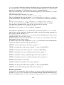
considerations by a number of options, e.g. input blocks 3b, 5, or 8. In this latter case great
care is needed, however, that the cell volumes are proportional to the volumes as seen by the
test flights for otherwise not only unscaled profiles, but even wrong (biased) profile shapes
will be obtained.
1.3.2.1
Scaling in problems with ignorable coordinates
As seen in the previous paragraph, the absolute values of estimates are scaled with the ratio
s/V of source strength to cell volume. Depending on ignorable coordinates in any particular
problem, or on whether stationary (i.e.: time is an ignorable coordinate) or time dependent
transport problems are considered , the dependent variable Ψ in the governing integral equation (1.1d), the source strength s and “cell volume” V may have different interpretations:
stationary (time independent) problems
one ignorable spatial coordinate In stationary problems with one ignorable coordinate,
say, the z-coordinate, the source strength s (input flag “FLUX”) is the flux, particles per
unit length dz in direction of z. Likewise, the volume V is per unit length in the ignorable
direction, i.e. if dz = 1 then V is the cell area in the two remaining coordinates x, y. The
unit length dz of an ignorable coordinate (here: z-coordinate) used in a particular run is
determined by the input flags in the corresponding input block for standard grid options, i.e.
in input block 2A for the x-coordinate, input block 2B for the y-coordinate and input block
2C for the z-coordinate, see Section 2.2. Note that the numerical value of source strength
“FLUX” (block 7) corresponds to the choice of e.g. dz. If dz = 1 cm, then “FLUX” is the
number of particles per unit time and per cm in z-direction. If dz = 1 m, then the same value
of variable “FLUX” would correspond to the 100 times smaller source strength of “FLUX”
particles per unit time and per meter. All resulting volume averaged output tallies would have
a value 100 times smaller. A particle density might then also be interpreted as surface density
(particle per unit area).
1.3.3
Statistical errors, Efficiency (FOM)
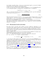
The efficiency for Monte Carlo Codes is the inverse of the figure of merit (FOM) of the
calculation, defined as
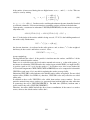
F OM = statistical variance · computing cost.
(3.23)
Note that FOM should be approximately independent of the running time, because the number of histories generated is (excluding overhead) proportional to the CPU costs and inversely
proportional to the statistical variance σ 2 .
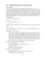
It is one of the major advantages of Monte Carlo methods over other numerical schemes that
the error estimates, empirical variances σ̃ 2 , are directly provided by the method itself, not
requiring any further considerations. The options to activate evaluation of statistical variance
in an EIRENE run for any computed quantity (tally) are described in input block 9 (section
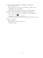
2.9). EIRENE provides numerical and graphical output for the “empirical relative standard
deviation”, in %.
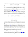
σ̃g,rel (N ) = σ̃g (N )/R̃g (N ) × 100
(3.24)
21