Download 4stack Processor's User Manual

4stack Processor’s User Manual
Bernd Paysan
25th April 2000
2
Introduction
The 4stack processor is a research project to create a high performance VLIW (very long
instruction word) microprocessor architecture without the typical disadvantages as uncompact code by using the stack paradigm for the individual operating units. Though the
restrictions of such a programming model, the processor will deliver highest integer and a
reasonable high floating point performance without excessive resource consumption such
as large decode and superscalar schedule logic.
3
4
Contents
1 Basic Programming Model
7
1.1
Stack Operations . . . . . . . . . . . . . . . . . . . . . . . . . . . . . . . .
7
1.2
Data Types . . . . . . . . . . . . . . . . . . . . . . . . . . . . . . . . . . .
8
1.3
Memory . . . . . . . . . . . . . . . . . . . . . . . . . . . . . . . . . . . . .
9
1.4
Register Files . . . . . . . . . . . . . . . . . . . . . . . . . . . . . . . . . .
9
1.5
Instruction Format . . . . . . . . . . . . . . . . . . . . . . . . . . . . . . .
11
2 Instruction Set Summary
13
2.1
Stack Operations . . . . . . . . . . . . . . . . . . . . . . . . . . . . . . . .
13
2.2
Data Move Operations . . . . . . . . . . . . . . . . . . . . . . . . . . . . .
19
2.2.1
Cache Control . . . . . . . . . . . . . . . . . . . . . . . . . . . . . .
20
2.2.2
MMU Control . . . . . . . . . . . . . . . . . . . . . . . . . . . . . .
21
2.2.3
I/O Control . . . . . . . . . . . . . . . . . . . . . . . . . . . . . . .
21
Flow Control . . . . . . . . . . . . . . . . . . . . . . . . . . . . . . . . . .
21
2.3
3 Programming Examples
23
3.1
Z–Buffer Drawing . . . . . . . . . . . . . . . . . . . . . . . . . . . . . . . .
23
3.2
Fixed Point Example: Fractals . . . . . . . . . . . . . . . . . . . . . . . . .
27
3.2.1
Fast Fourier Transformation . . . . . . . . . . . . . . . . . . . . . .
29
Floating Point Applications . . . . . . . . . . . . . . . . . . . . . . . . . .
32
3.3.1
Dot Product . . . . . . . . . . . . . . . . . . . . . . . . . . . . . . .
32
3.3.2
Floating Point Division and Square Root . . . . . . . . . . . . . . .
34
3.3.3
Denormalized floats . . . . . . . . . . . . . . . . . . . . . . . . . . .
37
3.3
5
6
CONTENTS
Chapter 1
Basic Programming Model
This chapter describes the application programming environment as seen by the assemblylanguage programmer. Architectural features that directly address the design and implementation of application programs are introduced. They consist of the following parts:
• Stack operations
• Data types
• Memory
• Register files
• Instruction format
1.1
Stack Operations
Stacks are pushdown lists with LIFO (last in first out) characteristic. The two elementary
operations are push (to store data) and pop (to fetch data). Pops read data in the reverse
order they were pushed before. Stack–type operations first pop an amount of data from
the stack, process these data and push the results back. To express these stack operation,
a stack effect is used. This stack effect addresses only the affected topmost part of the
stack. A Forth–like notation is used, as Forth is a stack language with a long tradition.
Each stack effect has a left side, the source operands; and a right side, the result operands;
separated by a long dash. Each stack entry is represented by a space separated name.
The topmost stack element (TOS, top of stack) is the rightmost element in the name list.
Example: the stack add has the following stack effect:
ab—c
where c is the sum of a and b.
7
8
CHAPTER 1. BASIC PROGRAMMING MODEL
If the stack was created by pushing 1, 2 and 3 (in this order), a is unified with 2, and b with
3. The result c then is 5, and the stack contains 1 (not affected) and 5 as TOS afterwards,
so the total stack effect is
123—15
To give a formal description of the processor’s instructions, each instruction is described by
a name, the stack effect (separated by colons) and the equations of the result (separated by
semicolons and terminated by a full stop). For the above example of add, the description
would be
add: a b — c: c = a + b.
Stack names may be either literals, then they represent constants, or names containing non–
literal characters, then they represent variables. Equal symbols represent equal variables.
Eg. the operation that duplicates the TOS, dup, is described as following:
dup: x — x x.
Each x stands for the same value, both on the left and the right side.
1.2
Data Types
The stack elements store only one unified data type: a 32 bit value. Interpretation of these
values are up to the instructions. 64 bit data is represented by two stack elements; if these
values have a significance order, the higher significant value is nearer to the top of stack.
Stack instructions either use 32 or 64 bit two’s complement signed or unsigned integers or
bit patterns, or 32 bit IEEE single or 64 bit IEEE double floats. Memory instructions load
and store bytes (8 bit), half words (16 bit), words (32 bit) and double words (64 bit).
For clarity, stack effects indicate the data type the operation assumes on the stack. The
first letters, the prefix of a stack element, signal the type of the data:
x
n
u
c
h
nb
snb
xdh
xdl
dh
dl
udh
udl
Any 32 bit pattern
32 bit two’s complement signed integer
32 bit unsigned integer
8 bit unsigned character
16 bit unsigned half word
n bit unsigned bit pattern
n bit two’s complement signed bit pattern
64 bit pattern, higher significant part
64 bit pattern, lower significant part
64 bit two’s complement signed integer, higher significant part
64 bit two’s complement signed integer, lower significant part
64 bit unsigned integer, higher significant part
64 bit unsigned integer, lower significant part
1.3. MEMORY
sf
fh
fl
bfd
9
32 bit IEEE single float
64 bit IEEE double float, higher significant part
64 bit IEEE double float, lower significant part
bit field descriptor
The 4stack processor uses two’s complement arithmetic for signed integers. Negative numbers are represented by the increment of the bit inversion of their absolute value. Two’s
complement has two important advantages (among from being widely used): different bit
patterns represent different numbers and when ignoring the sign bit, add and sub can be
used for unsigned numbers (except overflow conditions). For the last reason, there are two
overflow conditions: carry1 for unsigned arithmetics and overflow for signed.
1.3
Memory
Memory is a linear sequence of 8 bit bytes addressed by a 32 or 64 bit number (4 gigabytes
or 16 exabytes), called the physical memory address. Data with size greater one byte is
addressed by the first byte containing the data. All accesses should be size aligned, thus
a division of the address by the access size gives a zero remainder. Misaligned accesses
either lead to an exception or are supported by the memory interface unit which inserts
additional instructions to load the other part of the unaligned address. Misalinged accesses
should be supposed to be slower.
The 4stack processor supports big and little endian byte ordering. This is controlled by each
memory register set. Thus a program may use mixed little and big endian accesses. Big
endian accesses are propagated unchanged to the bus interface, little endian accesses are
either provided by xoring the address with the appropriate bit pattern (7 for byte accesses,
6 for half word accesses and 4 for word accesses) or by byte swapping (implementation
dependent).
Implementations of the 4stack processors designed for a workstation–like environment usually don’t use the physical memory for addressing the memory. They use a page level translation of the virtual memory address to the physical memory address. This translation is
done by TLBs (translation lookaside buffers) in hardware and by page tables in software.
Virtual memory also provides memory protection and controlled kernel entry points.
1.4
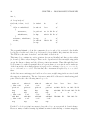
Register Files
There are four stacks for general purpose computations. Each stack allows direct access to
the 8 topmost values. Also, access to the 4 topmost values of any other stack is allowed:
1
The 4stack processor creates carry on subtract, not borrow, thus a carry set while subtracting means
“no overflow”
10
CHAPTER 1. BASIC PROGRAMMING MODEL
Stack 0 Stack 1 Stack 2 Stack 3
0s0
1s0
2s0
3s0
0s1
1s1
2s1
3s1
0s2
1s2
2s2
3s2
0s3
1s3
2s3
3s3
s4
s4
s4
s4
s5
s5
s5
s5
s6
s6
s6
s6
s7
s7
s7
s7
sr
sr
sr
sr
sp
sp
sp
sp
ip, index, loops, loope
Each element is addressed with it’s index. s0 is the top of stack, TOS, s1 the next of stack,
NOS, and so on. To address another stack, the stack number preceedes the stack index:
0s0 is the TOS of stack 0, 1s2 is the third element in stack 1.
Each stack has its on processing unit (ALU) and a status register (sr). The lower half of
the status register contains ALU specific information, the upper half contains the global
CPU state:
global state
per stack state
}|
{
z
}|
{ z
STAD0000 IIIIIIII CCCCCCCC 0UMMX0OC
S supervisor state
T trace mode
A address mode for instructions (0=32, 1=64 bits)
D activates external debugger
I
C
U
M
X
O
C
0
The
interrupt disabled
shift count (signed)
shift mode: 0=unsigned, 1=signed
rounding mode: 0=to nearest, 1=to zero, 2=to ∞, 3=to −∞
conditional execution (0=execute, 1=don’t execute)
overflow
carry
reserved and must be set to 0
UMMCCCCCCCC value is called the cm value and individually accessible.
Each stack has a stack pointer (sp), that points to the memory address where s0 will be
saved, when it would be spilled out. However, an access to the memory location of sp will
not give s0, because s0 is cached in a register file.
There are some global registers for special purposes:
The instruction pointer “ip” points to the next instruction, the loop counter “index”, the
loop start address “loops” and the loop end address “loope” are used by the hardware
do–loop instruction.
1.5. INSTRUCTION FORMAT
11
For memory access, there are two data move units. Each data unit is connected with two
stacks: one with the stacks with even number, the other with the odd stacks. Loads and
stores from the even data move unit can only go to or come from even stacks, from the
odd data move unit can go to or come from odd stacks.
Even stack unit
Odd stack unit
R0 N0 L0 F0
R0 N0 L0 F0
R1 N1 L1 F1
R1 N1 L1 F1
R2 N2 L2 F2
R2 N2 L2 F2
R3 N3 L3 F3
R3 N3 L3 F3
Each Rn contains one 32 (64) bit address. The corresponding Nn could be added to the
address to step through an array. Ln contains a modulo value to implement a ring buffer.
Fn contains usage flags:
00000000 00000000 00MMMMMM 000SBROZ
Z scale displacement (N, s0, constant offset) by size.
O byte order (0=big, 1=little endian).
R bit reverse addition.
B create bound crossing trap.
S stack usage: negate N on writes.
M limit mask bits, all M=0 means no limit.
For pipeline intermediate results, there exist some hidden registers, that have certain access
restrictions. Each of the two integer multipliers has one intermediate result latch called
mlatch. One mlatch is accessible by the lower stack half, stack 0 and 1, the other from
the higher stack half, stack 2 and 3. Values are stored with mul, umul and pass and
received with any sort of mul@ operations (speak “mul–fetch”). This restricts the usage
of the multiplier to only one per stack half and instruction. If there are two multiply
instructions per stack half, the result is undefined. It is not guaranteed that the behavior
of one implementation is valid for other implementations. Only if both pairs of operands
and both operations are equal, the result is specified.
The floating point operations store their arguments in the flatch registers, and their intermediate results in the fal and fml (floating point adder and multiplier latch) registers.
The intermediate result registers are readable from any stack, the argument registers are
divided into first and second argument. The first argument could be written by even stacks
(stack 0 and 2), the second argument by odd stacks (stack 1 and 3). The two adder argument latches could only be read by the lower stack half, the multiplier argument latches
by the upper stack half.
1.5
Instruction Format
The 4stack processor is a VLIW (very long instruction word) processor. This sort of
architectures exploit the fine grain parallelism of a program. Each long instruction word
12
CHAPTER 1. BASIC PROGRAMMING MODEL
consists of several operation fields for the independent execution units. All these operations
are performed simultaneous. It is up to the programmer or compiler to schedule the
individual operations to the instruction word.
The 4stack processor has 5 main instruction formats:
1. The normal instruction consists of four stack operations and two data move operations.
2. The conditional setup instruction consists of four stack operations and four corresponding conditional setup operations.
3. The branch instruction consists of four stack operations and one (conditional) branch
operation.
4. The call instruction consists of three stack operations and one ip–relative or absolute
call or jump instruction.
5. The far call instruction consists of one absolute call instruction.
Chapter 2
Instruction Set Summary
2.1
Stack Operations
Stack operations are divided into ALU operations and immediate number operations. The
immediate number operations are intented to push small numbers on the stack. They allow
either to push one sign extended 8 bit number or to shift the TOS by 8 bits to the left and
add one unsigned 8 bit number to the result:
s8b #: — s8b.
8b <#: n1 — n2: n2 = (n1 << 8) + 8b.
The ALU operations are used for general purpose and for floating point calculations. The
more important operations, add, sub, subr, addc, subc, subcr, or, and, xor, mul, umul and
pass have a second operand address that allows to access any of the addressable elements
of the stacks as second operand (thus 8 elements deep in the ALU’s own stack, 4 into any
other stack and 8 often needed constants).
The other operations need explicit use of the stack operation pick that uses all the stack
accesses from above operations except the 8 constants.
The second operand is further called NOS, for next of stack; although it might be any other
second operand addressed by the second operand address. The first operand is always the
top of stack, TOS, and therefore stated in the stack effect diagram.
The stack effect of one of the one–address operations then is: apply the stack effect of
the second operand address, pop NOS and (previous) TOS, apply the operation and push
the result — if any. The default stack effect stored in the instruction word is the swap
operation, that exchanges TOS and NOS; this stack effect will be used to describe the
operation.
The stack effects of the second operand addresses are:
13
14
CHAPTER 2. INSTRUCTION SET SUMMARY
s0: x — x x.
s1: x0 x1 — x0 x1 x0.
...
s7: x0 x1 x2 x3 x4 x5 x6 x7 — x0 x1 x2 x3 x4 x5 x6 x7 x0.
s0p:
s1p:
s2p:
s3p:
x0
x0
x0
x0
— x0.
x1 — x1 x0.
x1 x2 — x1 x2 x0.
x1 x2 x3 — x1 x2 x3 x0.
ns0:
ns1:
ns2:
ns3:
—
—
—
—
ns0.
ns1.
ns2.
ns3.
#0: — 0.
#−1: — −1.
#$7FFFFFFF: — $7FFFFFFF =
ˆ #max.
#$80000000: — $80000000 =
ˆ #min.
c0: — xc0.
c1: — xc1.
c2: — xc2.
c3: — xc3.
The following operations may use any of these second operand addresses:
or: x1 x2 — x3: x3 = x1 |x2 .
and: x1 x2 — x3: x3 = x1 &x2 .
xor: x1 x2 — x3: x3 = x1 ˆx2 .
add: n1 n2 / u1 u2 — n3 / u3: n3 = (n1 +n2 ); c = (u1 +u2 ≥ 232 ); o = (−231 ≤ n1 + n2 < 231 ).
sub: n1 n2 / u1 u2 — n3 / u3: n3 = (n1 −n2 ); c = (u1 −u2 ≥ 0); o = (−231 ≤ n1 − n2 < 231 ).
subr: n1 n2 / u1 u2 — n3 / u3: n3 = (n2 −n1 ); c = (u2 −u1 ≥ 0); o = (−231 ≤ n2 − n1 < 231 ).
addc: n1 n2 / u1 u2 — n3 / u3: n3 = (n1 + n2 + c); c = (u1 + u2 + c ≥ 232 ); o =
(−231 ≤ n1 + n2 + c < 231 ).
subc: n1 n2 / u1 u2 — n3 / u3: n3 = (n1 − n2 + c); c = (u1 − u2 + c ≥ 0); o =
(−231 ≤ n1 − n2 + c < 231 ).
subcr: n1 n2 / u1 u2 — n3 / u3: n3 = (n2 − n1 + c); c = (u2 − u1 + c ≥ 0); o =
(−231 ≤ n2 − n1 + c < 231 ).
pass: dl1 dh1 — : mlatch = d1 .
mul: n1 n2 — : mlatch = n1 ∗ n2 .
umul: u1 u2 — : mlatch = u1 ∗ u2 .
The operation pick may only use the stack addresses, not the constants. It allows to use
stack addresses without processing any operation, so the stack effect of pick is the stack
effect of its stack address.
2.1. STACK OPERATIONS
15
pick hstacki: —.
The operation pin pops the TOS and stores it to a deeper position in the stack:
pin
pin
pin
pin
pin
pin
pin
pin
s0:
s1:
s2:
s3:
s4:
s5:
s6:
s7:
x —.
x0 x1
x0 x1
x0 x1
x0 x1
x0 x1
x0 x1
x0 x1
— x1.
x2 — x2 x1.
x2 x3 — x3 x1 x2.
x2 x3 x4 — x4 x1 x2
x2 x3 x4 x5 — x5 x1
x2 x3 x4 x5 x6 — x6
x2 x3 x4 x5 x6 x7 —
x3.
x2 x3 x4.
x1 x2 x3 x4 x5.
x7 x1 x2 x3 x4 x5 x6.
There are some abbreviations for simple stack operations:
dup: x — x x =
ˆ pick s0.
over: x0 x1 — x0 x1 x0 =
ˆ pick s1.
swap: x0 x1 — x1 x0 =
ˆ pick s1p.
rot: x0 x1 x2 — x1 x2 x0 =
ˆ pick s2p.
drop: x — =
ˆ pin s0.
nip: x0 x1 — x1 =
ˆ pin s1.
There are also some abbreviation for unary operations that are performed using binary
operations with a special second operand:
nop: — =
ˆ or #0.
not: x1 — x2: x2 =∼ x2 =
ˆ xor #−1.
neg: n1 — n2: n2 = (−n1 ) =
ˆ subr #0.
inc: u1 — u2: u2 = (u1 + 1) =
ˆ sub #−1.
dec: u1 — u2: u2 = (u1 − 1) =
ˆ add #−1.
The rest of the stack instructions don’t have additional stack addresses.
The multiplication is a two cycle pipelined operation. The first part of the operation
(mul, umul and pass) allows various parameter addressing, the second part (all variations
of mul@) makes use of an additional adder (multiply and accumulate) a barrel shifter
and a rounder (for fractional integer arithmetics). If the shift count exceeds the range
−32 ≤ c < 32, the result is undefined.
mul@: — dl dh: d = mlatch.
mul<@: — dl dh: d = mlatch << c.
mulr@: — n: n = round(mlatch >> 32, m).
mulr<@: — n: n = round(mlatch << c − 32, m).
−mul@: — dl dh: d = −mlatch.
−mul<@: — dl dh: d = −mlatch << c.
−mulr@: — n: n = −round(mlatch >> 32, m).
−mulr<@: — n: n = −round(mlatch << c − 32, m).
mul@+: dl1 dh1 — dl2 dh2: c, d2 = d1 + mlatch, cc = cc + c.
mul<@+: dl1 dh1 — dl2 dh2: c, d2 = d1 + mlatch << c, cc = cc + c.
16
CHAPTER 2. INSTRUCTION SET SUMMARY
mulr@+: dl dh — n: c, n = round((d + mlatch) >> 32, m), cc = cc + c.
mulr<@+: dl dh — n: c, n = round((d + mlatch << c) >> 32, m), cc = cc + c.
−mul@+: dl1 dh1 — dl2 dh2: c, d2 = d1 − mlatch, cc = cc − ∼c.
−mul<@+: dl1 dh1 — dl2 dh2: c, d2 = d1 − mlatch << c, cc = cc − ∼c.
−mulr@+: dl dh — n: c, n = round((d − mlatch) >> 32, m), cc = cc − ∼c.
−mulr<@+: dl dh — n: c, n = round((d − mlatch << c) >> 32, m), cc = cc − ∼c.
Flag computation allows some branchless conditional computing. In the 4stack processor,
flags are computed using the TOS, carry and overflow flag of each stack. Flag computations
consume the TOS. A true flag has all its bits set (−1), a false flag has all its bits clear (0).
sub and subr compute the appropriate carry and overflow flag for compare flags. There is
one exception from this rule: double number operations like mul@ or fadd@ give zero only
if both 32 bit parts are zero, if the condition is asked in the same cycle.
t: x — −1.
0=: n — f: f = (n = 0).
0<: n — f: f = (n < 0).
ov: n — f: f = o.
u<: n — f: f = c.
u>: n — f: f = c ∧ (n 6= 0).
<: n — f: f = (n < 0) 6= o.
>: n — f: f = (n 6= 0) ∧ ((n < 0) = o).
f: n — 0.
0<>: n — f: f = (n 6= 0).
0>=: n — f: f = (n ≥ 0).
no: n — f: f = o.
u>=: n — f: f = c.
u<=: n — f: f = c ∨ (n = 0).
>=: n — f: f = ((n < 0) = o).
<=: n — f: f = (n = 0) ∨ ((n < 0) 6= o).
Although the barrel shifter in mul<@ provides a powerful bitwise shift instruction, there
are a number of simple shift instructions that shift only one position at a time. These
instructions are useful for some special purpose shifts and especially for simple divisions
and multiplications by two.
asr: n1 — n2: n2 = n1 >> 1; c = n1 &1; o = 0.
lsr: u1 — u2: u2 = u1 >> 1; c = u1 &1; o = 0.
ror: u1 — u2: u2 = (u1 >> 1)|(u1 << 31); c = u1 &1; o = 0.
rorc: u1 — u2: u2 = (u1 >> 1)|(c << 31); c = u1 &1; o = 0.
asl: n1 — n2: n2 = n1 << 1; c = (n1 >> 31)&1; o = (sign(n1 ) 6= sign(n2 )).
lsl: u1 — u2: u2 = u1 << 1; c = (u1 >> 31)&1; o = 0.
rol: u1 — u2: u2 = (u1 << 1)|(u1 >> 31); c = (u1 >> 31)&1; o = 0.
rolc: u1 — u2: u2 = (u1 << 1)|c; c = (u1 >> 31)&1; o = 0.
There are two bit operations, find first one and population count.
2.1. STACK OPERATIONS
17
ff1: x – n: n := 0; while(x&$80000000 = 0)do n := n + 1; x := x << 1; done.
popc: x – n: n := 0; while(x 6= 0)do n := n + (x&1); x := x >> 1; done.
Bytes and half words are loaded as unsigned integer parts. If they need to be interpreted
as signed integer or fraction parts, they have to be converted:
lob: u — b: b = u >> 24.
loh: u — h: h = u >> 16.
extb: b — n: n = (b ≥ $80)?b| − $80 : b).
exth: h — n: n = (h ≥ $8000)?h| − $8000 : h).
hib: b — n: n = b << 24.
hih: h — n: n = h << 16.
There are a number of instructions to address the special global or per stack registers. To
load these registers to the stack, the syntax hregisteri@ (speak “fetch”) is used, to store
them, hregisteri! (speak “store”) is used:
sr@: — x: x = sr.
sp@: — u: u = sp.
cm@: — b: b = ((sr >> 8) & $FF)|(sr << 4) & $700.
index@: — u: u = index.
loops@: — u: u = loops.
loope@: — u: u = loope.
ip@: — u: u = ip.
flatch@: — fl fh: f = f latch.
sr!: x — : sr = (s)?x : (sr&$FFFF0000)|(x&$FFFF).
sp!: u — : sp = u.
cm!: b — : sr = (sr&$FFFF008F)|((b & $FF) << 8)|(((b < 0?bˆ$300 : b) >> 4)&$70).
index!: u — : index = u.
loops!: u — : loops = u& − 8.
loope!: u — : loope = u& − 8.
ip!: u — : ip = u& − 8.
ip! doesn’t affect the next instruction; it is executed in the delay slot. The address of the
instruction after the next instruction is specified by the address applied to ip!. This is true
for loops! and loope! to some extend, too: There is a one cycle delay until the fetch unit
recognizes the new loop range addresses.
The 4stack processor has a floating point unit with a two cycle pipelined multiplier and a
two cycle pipelined adder. Floating point operations move the two topmost stack elements
to the unit’s input latches, from the unit’s output latches to the stack or from one unit’s
unnormalized output to the adder input. The last allows a three cycle multiply and add
and a single cycle accumulate. Once supplied with an input, the floating point units start
to compute the result.
fadd: fl fh — : f al = f .
fsub: fl fh — : f al = −f .
18
CHAPTER 2. INSTRUCTION SET SUMMARY
fmul: fl fh — : f ml = f .
fnmul: fl fh — : f ml = −f .
faddadd: — : f al = f ar.
faddsub: — : f al = −f ar.
fmuladd: — : f al = f mr.
fmulsub: — : f al = −f mr.
fi2f: n — : f al = $43300000, nˆ$80000000.
fni2f: n — : f al = $C3300000, nˆ$80000000.
fadd@: — fl fh: f = f ar.
fmul@: — fl fh: f = f mr.
fs2d: s — fl fh: f = s.
fd2s: fl fh — s: s = f .
fiscale: fl1 fh1 n — fl2 fh2: f2 = f1 ∗ 2n .
fxtract: fl1 fh1 — fl2 fh2 n: f2 = f1 /2n with 1 ≤ |f2 | < 2.
Some simple floating point instructions use the stack ALU:
fabs: fl1 fh1 — fl2 fh2: f2 = |f1 | =
ˆ and #$7FFFFFFF.
fneg: fl1 fh1 — fl2 fh2: f2 = −f1 =
ˆ xor #$80000000
f2∗: fl1 fh1 — fl2 fh2: f2 = f1 ∗ 2 =
ˆ add c3
f2/: fl1 fh1 — fl2 fh2: f2 = f1 ∗ 2 =
ˆ sub c3
The bit field instructions use a bit field descriptor (bfd). The format of the bfd is:
hrot left (r)i8 , hmask length (n)i8 , hmask rotation (m)i8 . All these values are interpreted
modulo the number of bits in a word.
bfu: x bfd — u: mask = rotl((1 << n) − 1), m); u = rotl(x, r)&mask.
bfs: x bfd — n: mask = rotl((1 << n) − 1), m); n = sign extend(rotl(x, r)&mask, r +
m + n).
cc@: – n: n = cc.
cc!: n –: cc = n.
The pixel pack and extract instructions transform pixel data into the next wider representation and back. 4, 8 and 16 bits per pixel are supported. The “,” operator means
concatenation. The pixel elements of the word are numerated from MSB to LSB.
px4: pn1 pn2 — dpb: dpb = (pn2 [0], pn1 [0]), (pn2 [1], pn1 [1]), (pn2 [2], pn1 [2]), (pn2 [3], pn1 [3]),
(pn2 [4], pn1 [4]), (pn2 [5], pn1 [5]), (pn2 [6], pn1 [6]), (pn2 [7], pn1 [7]).
px8: pb1 pb2 — dph: dph = (pb2 [0], pb1 [0]), (pb2 [1], pb1 [1]), (pb2 [2], pb1 [2]), (pb2 [3], pb1 [3]).
pp4: dpb — pn1 pn2: dpb = (pn2 [0], pn1 [0]), (pn2 [1], pn1 [1]), (pn2 [2], pn1 [2]), (pn2 [3], pn1 [3]),
(pn2 [4], pn1 [4]), (pn2 [5], pn1 [5]), (pn2 [6], pn1 [6]), (pn2 [7], pn1 [7]).
pp8: dph — pb1 pb2: dph = (pb2 [0], pb1 [0]), (pb2 [1], pb1 [1]), (pb2 [2], pb1 [2]), (pb2 [3], pb1 [3]).
2.2. DATA MOVE OPERATIONS
2.2
19
Data Move Operations
Data move operations are divided into load/store, address update and immediate offset
operations. An immediate offset operation in one data move field is added to the computed
address in the other data move field. Load and store operations may address one of four
register sets; as do update address operations. set and get may direct address any part of
the register set, the four registers R, N, M and F. Load operations have one delay slot, so
they push their result before the second instruction after the load starts execution.
Data move operations of the even data unit operate on one or both of the even stacks (stack
0 and 2), operations of the odd data unit on one or both of the odd stacks (stack 1 and
3). Both load and store operations may use one or two stacks as source or result. Update
address, set and get may only use one stack as source or result. The stack is specifield with
n: or n1 &n2 :, where n is the stack number of a single destination stack; n1 is the stack for
the value at the lower address, n2 is the stack for the value at the higher address. Stack 0
or stack 1 is the default stack.
Load and store operations allow a number of addressing modifiers:
syntax
Rn
Rn +N
Rn N+
Rn +N+
s0b
ipb
s0l
ipl
Rn +s0
Rn s0+
Rn +s0+
address
Rn+imm
Rn+Nn+imm
Rn+imm
Rn+Nn+imm
s0+imm
ip+imm
s0+imm
ip+imm
Rn+s0+imm
Rn+imm
Rn+s0+imm
Rn becomes
Rn
Rn
Rn+Nn
Rn+Nn
Rn
Rn
Rn
Rn
Rn
Rn+s0
Rn+s0
comment
indirect
indexed
modify after
modify before
stack indirect b.e.
ip relative b.e.
stack indirect l.e.
ip relative l.e.
stack indexed
stack modify after
stack modify before
The top of stack s0 is used from the only or the low address stack at the begin of the
operation.
The semantics of the operation “+” depends on the flags Fn. The index is the sum of the
second operand (if any) and the constant offset from the other data move unit.
Z set The index is shifted by the access size.
R set The index is added using bit reverse addition.
S set The index is negated if the instruction is a store (stack-like usage).
If the limit mask bit number is not 0, the base address Rn is split into a lower half (with
M bits), and an upper half (with 32 − M bits). The calculation is performed on the lower
20
CHAPTER 2. INSTRUCTION SET SUMMARY
half; if the result exceeds the limit register Ln, or causes a carry on the M th bit, it is set
to 0 and a bound crossing trap occurs, if B is set. The result of this comparison is added
to the upper half then. This is the final effective address that is propagated to the cache
to perform the memory access.
The store operations are stb, sth, st and st2/stf. stb stores the lower 8 bits of the
number(s) on the stack(s) specified at the end of the cycle. sth stores the lower 16 bits,
st stores the total 32 bit value and st2/stf stores a value pair. stf is an alias for st2.
Little endian accesses, when O is set, are computed by xoring 7, 6 and 4 for byte, half word
and word accesses. For double accesses, the relation lower/higher address is reversed, so
you specify the higher address first. Double word addresses are the same in big and little
endian.
The address update operation assings the sum or difference of one register, 0, it’s Nn, or
the TOS of the selected stack and the constant offset to one of the four registers. Syntax:
Rm= Rn [s:] [(+|−)(N|s0)]. There is no scaling by size, because no size is specified. The
source register’s flags are used for computing conditions.
set and get individually select one of the registers, Rn, Nn, Mn or Fn and set their value
to the TOS of the specified stack or get the register’s value and push it to the stack. setd
and getd do the same for 64 bit extended addressing — if not implemented, the higher half
is ignored when set and 0 when get.
2.2.1
Cache Control
The instructions ccheck, cclr, cstore, cflush, cload, calloc, and cxlock control the cache.
All these accesses use the address in Rn to select one cache line. The address part that is
used to address the cache line set in usual accesses is used here, too. The lower bits select
one line of the set. The higher bits are compared with the cache line’s address; the mask
count M specifies the lower bits of them not to compare. It is ensured that a walk with
constant offset through one page’s address range will select all cache lines. Bit 0–1 specify
which cache to check: data, instruction, lower stack’s and higher stack’s cache (even/odd
is selected by the operation slot).
Example: an implementation may have 4K pages and 32 byte cache lines in a four way set
associative cache. Thus, the lower 12 bit select the cache line. Therefrom the lower 5 bits
select way and cache: 0 is way 0, 8 is way 1, $10 is way 2 and $18 is way 3, all in data
cache.
ccheck returns the result of the check at the begin of the second instruction after its
issue. Thus it has a delay slot as any other cache access. The result contains the status
bits (shared/exclusive, modified and valid) of the cache line, a flag wether the compare
matched or failed, the number of unprocessed entries in the global write buffer and the
cache tag address. Checking the global write buffer helps to flush the cache without long
interrupt latency.
2.3. FLOW CONTROL
21
cclr clears a cache line, cstore writes a cache line, cflush writes and clears a cache line; these
three operations ignore the higher part of the address. cload starts a cache load to the
specified line, calloc allocates the cache line without changing the line entries and cxlock
changes the lock flag while ensuring that the specified cache line is loaded.
A cache flush does not ensure that the cache is empty after the flush, but it ensures that
cache and memory before the flush are consistent afterwards, thus all modified lines are
written out and any valid data in the cache contains the same values as the corresponding
memory. When interrupts are disabled, the cache is really empty, except those parts needed
to run the cache flush loop.
2.2.2
MMU Control
2.2.3
I/O Control
The operations out, outd, ins, ioq, inb, inh, in and ind control I/O ports. I/O accesses
are not cacheable and not translated by the memory management unit; even if they go
to memory addresses, and not to special port addresses. All I/O accesses are performed
strictly sequential in an I/O queue with an implementation dependend number of I/O
read/write buffers. The access use the address in Rn plus the immediate constant scaled
by 8. Each I/O read is a 64 bit read, each write is a 64 bit write to the corresponding
address. On a wider bus, the lowest valid bits in the address selects appropriate bus part.
The input start operation ins returns the number of one of an implemenation defined
amount of input latch register. The io query operation ioq returns true, if the passed
register number is filled, false otherwise. An inb, inh, in or ind operation reads the port
value and frees the latch register. The immediate offset allows to select the appropriate
byte/half word/word out of the double word read.
I/O accesses will cause a privilege violation exception when not processed in supervisor
mode.
2.3
Flow Control
Flow control operations divide into conditional branches, counted loops, calls/jumps, returns and indirect calls/jumps. Conditional branches use a ten bit branch offset that allows
to jump back 1024 instructions and 1023 instructions forth. Loops may use up to 1023
instructions as loop body. A call or jump may cover the entire 32 bit addressing space of
4 gigabytes (2 gigabytes forth or back); a far call the entire extended 64 bit addressing
space.
All flow control operations (except indirect jump/call with ip!) use the data move operation
field, so while executing flow control operations no data move operations can be executed
in parallel.
22
CHAPTER 2. INSTRUCTION SET SUMMARY
Conditional instructions are the most important flow control operations. The 4stack processor allows all four stacks to be checked for a specified condition and to jump if either
at least one or all of the specified stacks met the condition. This allows to combine some
conditions to one conditional jump.
Conditions may either pop the examined top of stack (then preceeded with a question
mark “?”) or leave it unchanged (preceeded with a colon “:”). The conditonal branch
operation br thus is followed by the specified stacks (more than one must be separated by
“|” for oring, by “&” for anding the condition), by the specified condition (t, 0=, 0<, ov,
u<, u>, <, >, f, 0<>, 0>=, no, u>=, u<=, >=, <=) preceeded with “?” or “:” and by
the branch target (usually a label). If no stack and no condition is specified, the branch is
unconditional.
Counted loops help to implement inner loops without branch overhead. The loop setup
operation do sets loops to the next instruction and loope to the label after the operation.
The loop index has to be set by the programmer with the instruction index!. The loop
continues until the loop index decrements from 0 to −1. The index is decremented in the
last cycle of every loop.
Calls (operation call) and jumps (operation jmp) transfer the program flow to the label
after the operation. Both use the operation field of stack 3. call executes ip@ on stack 3
to push the return address, jmp performs a nop on stack 3. Far calls execute nops on any
stack except on stack 3, there ip@ is executed.
The conditional setup operation allows some stacks to conditionally execute operations
without breaking the program flow. For each stack one condition is tested and if false, the
X bit in the status register of the corresponding stack is set and all following operations
on that stack are replaced by nops until another conditional setup changes the situation.
As in conditional branches, conditions may either pop or copy the top of stack, and are
preceeded with “?” or “:” to select that.
The conditions t and f have a special meaning: t resets the X bit and thus all operations
afterwards are executed, f inverts the X bit and therefore allows if–then–else. When set, no
other condition may change the state of the X bit of one stack. All conditions (regardless
of being part of a conditionnal setup operation or a conditional branch operation) read as
false. Stores and loads to that stack are aborted; address offsets s0 read as zero.
Indirect jumps are generated with ip!. They transfer program flow to the address on the
stack that executes ip!. Indirect calls may use any stack except stack 3 and have to save
the caller’s instruction pointer with ip@ on stack 3.
Chapter 3
Programming Examples
This chapter contains a number of programming examples which introduce into the programming of the 4stack processor. The examples are intented to show programming methods that exploit the parallelism of the algorithm and therefore produce fast and compact
code. The algorithms of the example programs target possible applications of the 4stack
processors: high speed graphic, integer signal processing and some floating point number
crunching.
3.1
Z–Buffer Drawing
Three dimensional drawing on a two dimensional CRT display has one problem: hidden
surfaces. A number of algorithms face to that problem. One simple and elegant solution
is z–buffering. Each pixel in the three dimensional space has x and y coordinates that
correspond to display coordinates. The z coordinate does not have any correspondence to
the display, but there is one condition for pixels on the screen: Only that one shows on
the screen, which has the highest z coordinate value of all the 3D pixel with the same x
and y coordinate. Therefore a z–buffer holds the actual z value for the pixel shown on any
screen position. New pixels are only drawn if their z value is interpreted as closer to the
screen than the actual z value.
Usually object surfaces are divided into flat areas. These areas then are drawn in horizontal
lines, as the frame buffer is organized in horizontal lines, too. A C code fragment for z–
buffer drawing may look like that:
unsigned short *zbuffer;
color *screen;
color c;
unsigned short z;
short dz;
23
24
CHAPTER 3. PROGRAMMING EXAMPLES
int i;
/* loop body */
for(i=0; i<len; i++)
{
if(z >= *zbuffer)
{
*screen=c;
*zbuffer=z;
}
screen++; zbuffer++;
z+=dz;
/* index!
do
*/
/* sub s1
?u>=
*/
/* pick s1
/* dup
st 0: R2 N+ */
sth 0: R1 N+ */
/* nop
/* add s2
/* nop
:t
ldh 0: R1
*/
*/
*/
}
The sequential 4stack code in the comments above is only a bit vectorized: the zbuffer
load is placed at the end of the loop. R1 is used to keep zbuffer, R2 points into the screen.
The TOS is z, the next of stack is c and the third of stack is dz.
This inner loop contains two active pointers (screen and zbuffer) and three active values
(z, dz and c), where only z changes. There are no dependencies between neighboring pixels
except the linear z change and the address pointer increments. Thus although this basic
block seems to be rather sequential, there is a great chance to vectorize it and to make use
of the four stacks. As z changes linear, it is proposed to exchange z by z0 = z, z1 = z + dz,
z2 = z + 2dz and z3 = z + 3dz. The last line, the z increment is replaced by zn = zn + 4dz
then.
As the data move unit supports double word accesses, neighboring pixels are stored with
the same store instruction. The two data move units hold addresses for interleaving pixel
pairs. This leads to the following inner loop code:
subr s1
;; 4dz c z0
pick s1
dup
nop
;; 4dz c z0
add 0s2
;; 4dz c z0’
nop
subr s1
c z2
pick s1
dup
nop
c z2
add 0s2
c z2’
nop
subr s1
c z1
pick s1
dup
nop
c z1
add 0s2
c z1’
nop
subr s1
c z3
pick s1
dup
nop
c z3
add 0s2
c z3’
nop
?u>=
?u>=
?u>=
?u>=
st 0&2: R2 N+ st 1&3: R2 N+
sth 0&2: R1 N+ sth 1&3: R1 N+
:t
:t
:t
:t
ldh 0&2: R1
ldh 1&3: R1
For the C code above it isn’t necessary to keep the color c on every stack; it doesn’t change.
However, many z–buffer drawing algorithms are mixed with shading or texture mapping.
3.1. Z–BUFFER DRAWING
25
There each pixel has a different color. So to make changes easy, the color is kept on every
stack.
This inner loop draws 4 z–buffered pixel every step (in 6 cycles). It would be very unpleasant, if every line length has to be a multiple of four. So for beginning and end of the loop,
the left respectively the right of the four pixel line piece must be masked out. This can
be done with the conditional setup, too, as conditional setup on disabled stacks doesn’t
change the X flag state. The startup then is:
0 #
sub 1s3
2 #
sub s3p
1 #
sub 1s3
3 #
sub 1s3
ldh 0&2: R1
?>=
?>=
ldh 1&3: R1
?>=
?>=
The third of stack on stack 1 contains the number of points to skip at the start (the rest
from dividing the start offset by 4). This code compares the starting index with 0 to 3 and
sets the X flag, if the number on the stack is less than the starting index. The z–buffer
load is included into this code sequence, the load is aborted, if the X flag is set.
At the end of the loop, the z–buffer value is just loaded and can’t be aborted. Thus the
order of masking points out is reversed:
subr s1
0 #
sub 2s3
;; c z0
pick s1
dup
nop
subr s1
2 #
sub 2s3
c z2
pick s1
dup
nop
subr s1
1 #
sub 2s3
c z1
pick s1
dup
nop
subr s1
3 #
sub 2s3
c r z3
pick s1
dup
nop
?u>=
;;
?<
?u>=
?u>=
?u>=
?<
?<
?<
st 0&2: R2 N+ st 1&3: R2 N+
sth 0&2: R1 N+ sth 1&3: R1 N+
:t
:t
:t
:t ;;
Here the third element of stack 2 contains the number of remaining pixel for the last iteration. It is compared with the numbers 0 to 3. Only smaller numbers will continue
execution. If the points wouldn’t be drawn anyway, because they are invisible, the comparison isn’t performed.
The complete code for one z–buffered line drawing is listed below. It must be noted, that
the return address has to be moved to a save place where it doesn’t disturb the computing
process.
;; 4dz
;; color
;; z
;; index
drawline:
index!
0 #
starti
color
z
nop
2 #
endi
color
z
nop
1 #
color
z
ret
swap
3 #
R1=zbuffer
R2=screen
N1=2
N2=2
R1=zbuffer
R2=screen
N1=2
N2=2
;;
ldh 0&2: R1
ldh 1&3: R1
26
sub 1s3
nop
;; dz c z’ zr
subr s1
;; dz c z’
pick s1
dup
nop
;; dz c z
add 0s2
nop
.loop
subr s1
0 #
sub 2s3
;; c z’
pick s1
dup
nop
;; dz c z
drop
drop
drop
CHAPTER 3. PROGRAMMING EXAMPLES
sub s3p
nop
c z’ zr
subr s1
c z’
pick s1
dup
nop
c z
add 0s2
nop
sub 1s3
nop
e c z’ zr
subr s1
e c z’
pick s1
dup
nop
e c z
add 0s2
nop
sub 1s3 ?>=
?>=
nop
do
c r z’ zr
subr s1 ?u>=
?u>=
c r z’
pick s2 st 0&2: R2 N+
dup
sth 0&2: R1 N+
nop
:t
:t
c r z
add 0s2 ldh 0&2: R1
nop
;;
subr s1
2 #
sub 2s3
c z’
pick s1
dup
nop
c z
drop
drop
nop
subr s1
1 #
sub 2s3
e c z’
pick s1
dup
nop
e c z
drop
drop
drop
subr s1
3 #
sub 2s3
c r z’
pick s2
dup
nop
c r z
drop
ret
drop
?u>=
;;
?<
?>=
?>=
?u>=
?u>=
st 1&3: R2 N+
sth 1&3: R1 N+
:t
:t ;;
ldh 1&3: R1 ;;
?u>=
?u>=
?u>=
?<
?<
?<
st 0&2: R2 N+ st 1&3: R2 N+
sth 0&2: R1 N+ sth 1&3: R1 N+
:t
:t
:t
:t ;;
;;
;;
Simply drawing flat shaded polygons is not very satisfying. Therefore at least Gouraud
shading should be applied to fill a polygon. Gouraud shading is a bilinear interpolation
between the edges of a polygon. This removes the most unpleasant color discontinuities at
the borders of the polygons. The basic line loop therefore has to increment or decrement
the color each drawing step. This changes the loop body to the following (in C and linear
4stack assembly code):
/* loop body */
for(i=0; i<len; i++)
{
if(z >= *zbuffer)
{
*screen=c;
*zbuffer=z;
}
screen++; zbuffer++;
z+=dz;
color+=dcolor;
/* index!
do
*/
/* sub s1
?u>=
*/
/* pick s1
/* dup
st 0: R2 N+ */
sth 0: R1 N+ */
/* nop
/* add s2
/* pick s3
:t
*/
*/
*/
3.2. FIXED POINT EXAMPLE: FRACTALS
/* add s2
/* pin s2
}
ldh 0: R1
27
*/
*/
As Gouraud shading does not produce overflows, a normal add is sufficient. However,
accuracy is not very high, since true color screens usually represent colors by a set of 3
8 bit values in the format αRGB and therefore each color scales only between the integer
values of 0 to 255. For larger polygons this differential increment is not very good, for
small polygons, it can be tolerated.
While unrolling this part of the loop, we get a small amount of additional accuracy: as
with dz, we add 4 ∗ dcolor each iteration. The final loop body then is:
;; dz c z’ zr
subr s1
;; dz c z’
pick s1
dup
nop
;; dz c z
add 0s2
pick 1s2
;; dz c z dc
add s2
;; dz c z c’
pin s2
;; dz c’ z
dc c z’ zr
subr s1
dc c z’
pick s1
dup
nop
dc c z
add 0s2
pick 1s2
dc c z dc
add s2
dc c z c’
pin s2
dc c’ z
e c z’ zr
subr s1
e c z’
pick s1
dup
nop
e c z
add 0s2
pick 1s2
e c z dc
add s2
e c z c’
pin s2
e c’ z
c r z’ zr
subr s1 ?u>=
?u>=
c r z’
pick s2 st 0&2: R2 N+
dup
sth 0&2: R1 N+
nop
:t
:t
c r z
add 0s2 ;;
pick 1s2 ;;
c r z dc
add s3
ldh 0&2: R1
c r d c’
pin s3
;;
c’ r d
?u>=
?u>=
st 1&3: R2 N+
sth 1&3: R1 N+
:t
:t ;;
ldh 1&3: R1
This code allows to draw Gouraud shaded, z–buffered polygons at a peak rate of 2 cycles
per pixel.
3.2
Fixed Point Example: Fractals
A very popular benchmark program is drawing fractals like the Mandelbrot set. This
set contains elements of the complex number set C that fit the condition:
M = {c0 | lim |ci | < 2 with ci+1 = c2i + c0 }
i→∞
To get nice colored picture, the number of iterations until the number becomes bigger than
2 is counted and for each number a different color is selected.
This code has some strict conditions that don’t allow easy vectorization: It is an iteration;
the value computed in one step is used in the next. However, it contains enough inner
parallelism to fill all the instruction slots.
28
CHAPTER 3. PROGRAMMING EXAMPLES
First, we have to transform the complex calculation into real and imaginary parts (x is the
real part of c, y the imaginary part):
c2 = x2 − y 2 + 2ixy
|c| =
q
x2 + y 2
(|c| < 2) = (|c|2 < 4) = (x2 + y 2 < 4)
For speed, we want to use fractional integer arithmetics. The problem fits quite well to
the restrictions of fractional integer arithmetics: the interesting part of the Mandelbrot
set is between -2 and 2 for both complex and real coordinates. The part close to 0 is not
very interesting, because it is all in the set. So the interesting part of the Mandelbrot
set does not even span an order of magnitude. Therefore the magnitude (the exponent)
of a floating point number would not change much during the calculation process. 32 bit
fractional integer arithmetics thus provides more accuracy than single precision floating
point.
Now we have to separate the multiplications. We need x2 , y 2 and 2xy; three multiplications.
However, we need to calculate x2 −y 2 and x2 +y 2 , and the multiply and accumulate doesn’t
allow to compute this both results at once. So we compute −2x2 and add x2 − y 2 to it, so
we finally get −x2 − y 2 , for sacrifying some small bits of accuracy:
iterloop:
;; x
n
y
mul s0
pick 2s0
mul 0s0
;; x
n y
y
mul<@
mul s0
mulr<@
;; x dx2
n
y 2xy
-mulr<@+ dec
add s1
;; x x2+y2 n-1
y 2xy+y
add s1
dup
nop
;; x x+x2+y2
;;
n-1 (n-1>=0)
;;
y 2xy+y
pick 0s0
x
mul s0
d4
-mulr<@+
4-2x2
add 0s0
.ip.d: four # ld2 3: ipb
br 1&3 ?0>= iterloop
(4-x2-y2>=0)
The final branch branches to iterloop, while the square of the absolute value of |c|2 =
x2 + y 2 < 4 and the iteration count n ≥ 0.
3.2. FIXED POINT EXAMPLE: FRACTALS
3.2.1
29
Fast Fourier Transformation
One important function for digital signal processing is the fast Fourier transformation
FFT. It transforms a complex, time discrete sample into a complex spectrum with discrete
frequencies. This discrete frequencies are called Fourier coefficients Ck (f )1 :
Ck (f ) :=
Z1
f (t)e−2πikt dt,
k∈Z
0
For discrete samples (n samples for f (t), δt = const.) only the first n coefficients Ck (f ) are
of interest. It is easy to show that Ck+zn (f ) = Ck (f ), z ∈ Z in this case (aliasing).
Cooley & Turkey showed in 1965, that for n = 2p only np/2 complex additions, subtractions
and multiplications, and n trigonometric coefficients are necessary to compute a complete
Fourier transformation (fast Cooley & Turkey Fourier transformation, FFT).
The main principle of FFT is a recursive divide and conquer strategy. The input is divided
into even and odd parts, each of them are processed in the same way separate, and combined
afterwards. In practice, all divide steps are performed at once: consecutive dividing the
input array into even and odd bit–reverses the access indices. The 4stack processor has a
dedicated address adding mode for this sort of access, that allows to process consecutive
(or at a constant offset) bit–reverse addressed elements of an array.
The combination part is also usually not recursively processed; a loop rearrangement allows
to reuse the trigonometric coefficients and therefore reduces memory bandwidth.
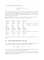
The body of the combination part is called “butterfly diagram”:
ck := ck + ck+m ∗ eiπj/m ||ck+m := ck − ck+m ∗ eiπj/m
ck
c k+m
i π j/m
* e
+
-
Figure 3.1: Butterfly diagram
The realization of the butterfly diagram results in the complex multiplication of ck+m
and eiπj/m and the addition and subtraction from ck ; looping for all 0 ≤ j < m and all
j ≤ k < n, step 2m. The conversion from complex to real equations leads to:
1
See for example Skriptum zur Vorlesung Numerik I und II, C. Reinsch
30
CHAPTER 3. PROGRAMMING EXAMPLES
f.r := cos πj/m||f.i := sin πj/m
h.r := c.rk+m ||h.i := c.ik+m
h.r := h.r ∗ f.r − h.i ∗ c.i||h.i := h.r ∗ f.i + h.i ∗ f.r
c.rk := c.rk + h.r||c.ik := c.ik + h.i||c.rk+m := c.rk+m − h.r||c.ik+m := c.ik+m − h.i
Arranging the loops with constant j in the inner loop makes the first assignment loop
invariant. It further turns out that the second assignment and the fourth have a swap
type parallelism; the fourth read h, the second writes to h, so for loop unrolling the second
equation can be executed in parallel with the fourth. Now only two sequential assignment
lines remain in the inner loop:
;; fr
pick 3s0
;; fr hr
hi
mul 0s0
--
fi
pick 1s0
fi hi
hr
mul 0s0
--
mul 2s1
;; fr gi
mul@
2:hifr/2
mul s1
fi gr
mul@
2:hrfr/2
asr
;; fr gi/2
;;
mulr@+
asr
(hifr+fihr)/2=:qi
fi gr/2
add 1s0
subr 0s0
;; fr [qi+gi/2]
;;
[qi-gi/2]
-mulr@+
ld 2&0: R1
0 #
0 #
ld 3&1: R1 +N
(hrfr-hifi)/2=:qr
add 3s0
subr 2s0 st 2&0: R1 N+
fi [qr+gr/2]
[qr-gr/2]
st 3&1: R1 N+
It should be noted further, that FFT needs a final scaling by 1/ ld n, either in the FFT
case or in the reverse FFT case. For integer FFTs the best place to do the scaling is
the FFT procedure, because it ensures that no values will be out of range. The fixed
point multiplication has the implicit property to divide the result by two, and the asr
instructions does so for the ck . For reverse FFT the barrel shifter can be used to provide
a non halfing fixed point multiplication.
The middle loop has to step through the j index and thus complete the access to every
array element. Remember that all array accesses are bit reverse for FFT (the result is
obtained by a bit reverse address walk through the input array):
.begin
;; j
;;
n/2m
8n n/2m
<m> || 0
3.2. FIXED POINT EXAMPLE: FRACTALS
31
nop
sub c1
nop
drop
ld 0&2: R2 N+
ld 3&1: R1 +s0+
;; j
n/2m-2
8n n/2m -nop
index!
swap
pick 2s1 DO
;; j-k fr
hi
n/2m 8n fi
;;
8n hr
;; ... the inner loop, see above
.loop
;; fr
hi
fi
hr
pick 3s0 mul 0s0
pick 1s0 mul 0s0
ld 2&0: R1
0 #
;; fr hr
-fi hi
-mul 2s1
mul@
mul s1p
mul@
?t :t :t :t
;; gi
2:hifr/2
gr
2:hrfr/2
asr
mulr@+
asr
-mulr@+
;; gi/2
(hifr+fihr)/2=:qi
;;
gr/2
(hrfr-hifi)/2=:qr
add 1s0
subr 0s0
add 3s0
subr 2s0 st 2&0: R1 N+
st 3&1: R1 N+
;; the final loop step that doesn’t load another c_k+m value
;; j-k
nop
;; j-k
dec
;; j-k-1
-nop
-pick 2s0
n/2m
n/2m 8n
swap
8n n/2m
nop
8n n/2m
8n
drop
-0 #
0
R1= R1 2: +s0
R1= R1 3: +s0
br 0 :> .until
The outer loop then has to loop through m which scales from 1..n/2 while doubling each
step. The above cited <m> is the bitwise mirrored m by a bit length of ld n; thus it is n/2m.
.begin
nop
nop
pick 3s0 pick 3s0 set 2: N1
;; j
-8n n/2m
n/m
dup
pick 2s0
pick 2s0 pick 2s0 set 2: N2 ;;
;; j j
n/2m
8n n/2m
n/m <m>=n/2m
;; ... the middle loop (see above)
;; j 0
n/2m
8n n/2m
n/m 0
drop
2 #
asr
drop
R1= R3
;; j
n/2m 2
8n n/4m
n/m
asl
subr
nop
asr
br 1 ?> .until
;; 2j
-8n n/4m
n/2m
set 3: N1 ;;
R1= R3
;;
For the final loop f := eiπj/m is no longer loop invariant, it changes every step. IF n/2m
is not compared if > 1, but > 2, the final loop could be separated. A small modification
allows to process the last loop in 4 cycles per loop step, reducing the overhead of 4 cycles
per middle loop. A tiny trick allows to consume the f.r value without an additional drop
instruction:
32
CHAPTER 3. PROGRAMMING EXAMPLES
;; final loop
;; fr
hi
pick 3s0 mul 0s0
;; fr hr
--
fi
pick 1s0
fi hi
hr
mul 0s0
--
mul 2s1
;; gi
mul@
2:hifr/2
mul s1p
gr
mul@
2:hrfr/2
asr
;; fr gi/2
;;
mulr@+
asr
-mulr@+
ld 0&2: R2 N+
(hifr+fihr)/2=:qi
gr/2
(hrfr-hifi)/2=:qr
ld 3&1: R1 +N
subr 0s0
st 3&1: R1 N+
add 1s0
add 3s0
subr 2s0
ld 2&0: R1
0 #
?t :t :t :t ;; drops fr
st 2&0: R1 N+
This example shows the change of active values in loop computing. Each nested loop has
other active values. The inner loop operates on complex numbers, the outer loops do index
and address computation. Concentrating on the actual part helps to understand the work
being done. The inactive variables disappear in the stack diagrams. Sometimes they show
up at the edges of a inner part and have to be cleaned up. Unlike conventional register
architectures, this cleaning up has do be done in the code, not only in the mind of the
programmer or compiler.
3.3
Floating Point Applications
The 4stack processor’s application target is not excessive floating point computation; the
main applications are integer and fixed point computation as in graphics and signal processing. Therefore the number of parallel executed floating point instructions is less than
integer units: the 4stack processor issues one floating point multiplication and one floating
point add in parallel per cycle. Both result values can be forwarded to the floating point
adder; this reduces the adder latency from two to one cycle.
3.3.1
Dot Product
A basic operation on vector and matrix computation is the dot product
a·b=
n
X
ai b i
i=1
This simple operation shows how to make use of the floating point pipeline. A single load,
multiply and add would look like this:
3.3. FLOATING POINT APPLICATIONS
;; -nop
nop
;; ai
fmul
;; -nop
;; -nop
;; --
-nop
nop
bi
fmul
-nop
-nop
--
-nop
nop
-nop
-fmuladd
-nop
--
fsum
nop
nop
fsum
nop
fsum
fadd
-fadd@
fsum
33
ldf 0: R1 N+
ldf 1: R1 N+
This code is very slow and leaves many instruction slots empty. Thus, a full pipelined
version is:
;; count
dotp:
pick 3s0
nip
nop
fmul
fmul
fmul
.loop
fmul
fmul
ip!
fadd@
;; fresult
--
--
--
R1=v1
loops@
index@
nop
fmul
fmul
fmul
5 #
subr 0s1
index!
nop
fmuladd
fmuladd
loope@
nop
0 #
0 #
fadd
faddadd
ldf
ldf
ldf
ldf
do
ldf
fmul
fmul
index!
loops!
fmuladd
fmuladd
fmuladd
drop
faddadd
faddadd
faddadd
loope!
0:
0:
0:
0:
R1=v2
R1
R1
R1
R1
N+
N+
N+
N+
0: R1 N+
ldf
ldf
ldf
ldf
1:
1:
1:
1:
R1
R1
R1
R1
N+
N+
N+
N+
ldf 1: R1 N+
Although the inner loop contains only one instruction, there is a 4 step pipeline:
1. the element’s addresses are computed
2. the cache loads are done.
3. the multiplication is started
4. the multiply and adder result are forwarded to the adder input and another unnormalized sum is computed
The final step normalizes the sum. There must be at least 3 address computations, 2 loads
and one multiplication start before the loop can start. However, the DO operation doesn’t
allow a parallel load, so there must be one extra load in advance, and the first faddadd
must be replaced by a fadd of 0.0 to clear the second adder input latch.
34
3.3.2
CHAPTER 3. PROGRAMMING EXAMPLES
Floating Point Division and Square Root
The 4stack instruction set doesn’t contain neither a floating point division nor a floating
point square root. These instructions have been omitted, whilest silicon implementations
exist, because there is only a minor speedup with these hardware division or square root
devices, if these are implemented in an excessive way (at least 4 bits per cycle).
Goldschmidt’s algorithm should be used for both, the division and the square root. The
traditional algorithm, Newton–Raphson’s has more dependencies in each iteration step,
and surprisingly converts a bit slower in reality, while both have a theoretical conversion
rate of doubling the number of accurate digits each iteration.
Goldschmidt’s approximation uses three iteration variables, and thus allow enough parallelism to keep the pipeline filled (at least for division). The relative error is computed
each time by using subtraction instead of division to get the reziprocal of the relative error.
Division, computes a/b:
x := a, y := b, r :≈ 1/b
while y 6= 1 do x := rx, y := ry, r := 2 − ry;
As an approximation table would only contain reziprocal approximations for numbers
between 1 and 2, sign and exponent of y should be transferred to x before:
$20 div-table
bfd5:
.int $0511
.align 3
fdiv:
fdivgs:
;; bl bh
-fxtract
pick 0s0
;; yl yh bx bh
drop
and #min
;; yl yh
bs
fabs
0 #
;; yl yh
bs 0
nop
$40 #
;; yl yh
bs 0 $40
nop
hib
;; yl yh
bs 2.0
al ah
nop
al ah
pick 0s0
al ah bx
neg
al ah -bx
fiscale
xl xh
xor 1s2
xl xh
-pick 0s0 .ip.w# bfd5 ld 3: ipb
bh
ip@
0 #
set 3: R3
bh bfd5
bfu
bfrac[1:5]
drop
-$23 #
ldf 3: R3 +s0
-nop
--
;; y
fmul
;; --
x
nop
x
r
fmul
--
2.0
fadd
bs
3.3. FLOATING POINT APPLICATIONS
fmulsub
;; -fadd@
;; r
drop
-fmul@
x
fmul
-nop
--
fmul@
y
nop
y
;; r
fmul
fmul@
nop
x
nop
fmul
fadd@
-nop
fmulsub
fmul@
y
fmul
nop
nop
;; y
fmul
fmulsub
nop
r
fmul
nop
fadd@
x
nop
fmul
fmul@
-nop
nop
nop
;; -nop
fmul@
;; a/b
r
fmul
nop
--
x
fmul
nop
--
-ret
nop
--
35
The division table contains 32 reziprocal values, containing 64/(2j + 65):
.macro div-table [F] ( n -- )
1e0 fdup dup 2* s>d d>f f/ f+
dup 0 DO 1e0 fover f/ double,
1e0 dup s>d d>f f/ f+
.end-macro
LOOP
fdrop drop
The same approach can be done for the square root.
√
Square root, computes a:
√
x := a, y := a, r :≈ 1/ a
while y 6= 1 do x := rx, y := r2 y, r := (3 − r2 y)/2;
$20 sqrt-table
.double 1e0
sqrt-2
bfd5:
.int $511
.align 3
fsqrt:
36
CHAPTER 3. PROGRAMMING EXAMPLES
fsqrtgs:
fxtract
1 #
and
drop
f2/
$3FF8 ##
#,
hih
pick 0s0
xor s0
;; y
fmul
fmul@
fmul
fmulsub
fadd@
1:sqrt(2) x
swap
nop
fmul
fmul
nop
fmul@
fadd
fmul
fmul@
nop
r
fmul
flatch@
fmul
fmul@
nop
;; r
fmul
nop
nop
fmulsub
fadd@
x
nop
fmul
fmul@
nop
nop
-nop
nop
nop
nop
nop
y
fmul
fmul@
fmul
fmul@
nop
;; r
fmul
nop
nop
fmulsub
fadd@
x
nop
fmul
fmul@
nop
nop
-nop
nop
nop
nop
nop
y
fmul
fmul@
fmul
nop
nop
fmul
fmul@
;; sqrt(a)
fmul
nop
--
nop
nop
--
ret
nop
--
pick 0s1
pick 0s1
pick 0s1
asr
fiscale
pick 0s0
ip@
bfu
drop
nop
.ip.w# bfd5 ld 3: ipb
0 #
set 3: R3
-$25 #
-$5 #
;;
ldf 3: R3 +s0
ldf 1: R3 +s0
The square root approximation table contains reciprocal square roots for 32 numbers between 1 and 2; in fact the square roots of the division table.
.macro sqrt-table [F] ( n -- )
1e0 fdup dup 2* s>d d>f f/ f+
dup 0 DO fdup fsqrt 1e0 fswap f/ double,
1e0 dup s>d d>f f/ f+ LOOP fdrop drop
.end-macro
For square roots of numbers with odd exponent, the square root of 2 has to be multiplied
to the result, that’s the reason for the sqrt-2–macro.
3.3. FLOATING POINT APPLICATIONS
37
.macro sqrt-2 [F]
2e0 fsqrt double,
.end-macro
The number of iterations can be reduced by one if the approximation table sqares (thus
twice as many bits in the table index). This gives a space-time tradeoff. The tables would
be 8K instead of 128 bytes. While 8K can reside in the data cache, it is likely that the
values are spilled out or spill out other, important memory cells. However, it could be
worthful in both typical situations: When division and square root are used heavily, the
approximation table stays in the L1 cache and supports low latency divide and square root.
When they are used only from time to time, not much cache is wasted though (because
the approximation table has no chance to stay), and the L2 access times may be below the
spared iteration.
Note: a typical usage pattern of division and square root is to divide by the square root
of a number, thus as in vector norming:
(a, b, c)T := √
(x, y, z)T
x2 + y 2 + z 2
In this case, compute the reziprocal sqare root with a modified Goldschmidt’s algorithm,
and multiply the result to each x, y and z. Reziprocal square root does not take longer
than square root, and thus is clearly faster than square root following by division. In fact,
Goldschmidt’s square root algorithm allows to divide any number by the square root of
another number. But because square root divide is more expensive than multiplication, in
the usual vector norming application computing reziprocal sqare root and multiplying is
better.
√
Reziprocal square root, computes b/ a:
√
x := b, y := a, r :≈ 1/ a
while y 6= 1 do x := rx, y := r2 y, r := (3 − r2 y)/2;
3.3.3
Denormalized floats
The 4stack floating point unit doesn’t define denormal handling, while IEEE 754 requires it.
Implementations that don’t implement denormal handling may react in two fashions: either
denormal handling is disabled, then they treat denormalized values as zero; or denormal
handling is enabled, then they trap to the unimplemented floating point error. It is now
up to the exception handler to perform the correct operations to handle denormal floats.
Denormal floats processing can be emulated with instructions for normalized floats. The
purpose for denormalized floats is to fill in the hole between zero and the smallest normalized floating point number. So a simple shift of the exponent allows to compute normalized
38
CHAPTER 3. PROGRAMMING EXAMPLES
numbers, and a add with the appropriate value turns this into the same representation as
a denormalized value, except the exponent value. A multiplication of a normalized (a) and
a denormalized (b) value, where b is represented as + b, thus looks like:
a ∗ b = (a ∗ ((b + m) ∗ 264 − m ∗ 264 ) + m ∗ 264 )/264 − m
The final correction is only necessary, if the result is a denormal, too, and in this case,
don’t really perform the −m, because the value is already in denormal representation. The
result is a denormal, if the exponent is ≤ 64.