Download NOISE ANALYSIS USER MANUAL

NOISE ANALYSIS
USER MANUAL
Industrielle Meß-
und Prüftechnik
(P) 12/07/2004
Contents
1
The Rotas Noise Analysis System ................................................................................... 5
2
Basics of Noise Analysis ................................................................................................... 6
3
The Rotas-PC.................................................................................................................... 7
3.1
3.2
4
Assembly..................................................................................................................... 7
Electrical connections (schematic representation) ................................................. 8
Switching the PC ON and OFF....................................................................................... 8
4.1
4.2
5
Start the PC:............................................................................................................... 8
Shut down the PC ...................................................................................................... 8
Starting ROTAS ............................................................................................................... 9
5.1
5.2
5.3
ROTAS 2nd window ................................................................................................... 9
The Status bar.......................................................................................................... 10
Print graphics........................................................................................................... 10
6
ROTAS System Configuration...................................................................................... 11
7
The Toolbar .................................................................................................................... 11
8
The „Traffic light“ ......................................................................................................... 12
9
Supervising the test cycle............................................................................................... 13
9.1 Test Status ................................................................................................................ 13
9.2 Rotational Speed Display ........................................................................................ 13
9.3 Start- and Stop values ............................................................................................. 14
9.4 Command Orientated Control of the Test Cycle.................................................. 15
9.4.1
Supervise and test serial communication ........................................................... 15
9.4.2
Overview of the most important commands ...................................................... 16
9.4.3
Example of a command sequence ...................................................................... 18
9.5 Bit-orientated control of a test cycle ...................................................................... 19
9.5.1
The “Main Window” of the Parallel Control Unit ............................................. 19
9.5.2
Supervising and manipulating single bits........................................................... 20
9.5.3
Manipulating functional values.......................................................................... 20
9.5.4
Simulation and monitor mode ............................................................................ 21
9.5.5
Example of a test cycle on a gear tester ............................................................. 22
10
The ‚Scope’-Displays.................................................................................................. 25
10.1
10.2
Setting the Scaling, Zoom.................................................................................... 25
Panes and Labels.................................................................................................. 26
10.3 The Functions of the Function Buttons ................................................................. 26
10.4
Display Options .................................................................................................... 27
10.4.1
Rectangular Display or Display Polygons...................................................... 27
DISCOM
Noise Analysis User Manual
Page 2 of 63
10.4.2
Further Options............................................................................................... 27
10.5
Print the Scope ..................................................................................................... 28
10.6
Spectrogram-Display ........................................................................................... 28
10.7
Relative and Absolute Scaling of the x-Axis ...................................................... 29
10.8
Problems with the scope display......................................................................... 30
10.9
Tracking values of single orders......................................................................... 31
11
Measurement results .................................................................................................. 32
11.1
11.2
11.3
11.4
11.5
12
Table window ....................................................................................................... 32
Report window ..................................................................................................... 32
Report printing..................................................................................................... 33
Request One-Time Long Report......................................................................... 34
Storing Measurements in an Archive................................................................. 35
Measurement type definitions ................................................................................... 36
12.1
12.2
12.3
12.4
13
Measurement types from the time signal........................................................... 36
The “Dentist” and mesh order............................................................................ 37
Measurement types from the order spectrum: Harmonics and limit curves 38
Tracking values of single orders......................................................................... 39
Learning Limit Values ............................................................................................... 40
13.1
13.2
14
How the Limit Values are generated.................................................................. 40
Controlling the Learning Process....................................................................... 41
Testing a new Candidate Type.................................................................................. 42
14.1
How to create a new Candidate Type ................................................................ 42
14.2
Initial settings / learning of a new type of gearbox ........................................... 44
14.2.1
Switching the Hats on and off in ROTAS ...................................................... 45
15
How to Use the Statistics Database........................................................................... 46
15.1
15.2
15.3
15.4
15.5
15.6
16
Controlling the report database ............................................................................. 46
Creating Evaluations ........................................................................................... 47
Reproducible Measurements, Reference Measurements and Calibration..... 48
How to make reproducible measurements ........................................................ 49
Reference candidates ........................................................................................... 50
Calibration............................................................................................................ 50
Backup, Organisation of the Rotas Software........................................................... 51
16.1
16.2
16.3
16.4
17
Hard Disk Folders; range of a backup............................................................... 51
Organisation of files and folders......................................................................... 52
Making a backup copy......................................................................................... 54
Re-storing of a backup copy; Installation of Updates ...................................... 54
Appendix ..................................................................................................................... 56
17.1
Complete list of the possible commands from a test bench.............................. 56
17.1.1
Exchange of information about the candidate ................................................ 56
17.1.2
Controlling the Test Cycle (Test Step, Measuring)........................................ 57
17.1.3
Receiving Further Information ....................................................................... 58
17.1.4
Read Out Rotas Defect Information and Evaluation Result........................... 59
DISCOM
Noise Analysis User Manual
Page 3 of 63
17.1.5
17.1.6
17.1.7
17.1.8
17.1.9
DISCOM
Read out Rotas Values.................................................................................... 60
Displaying Messages ...................................................................................... 60
Controlling Gear Shift Force Measurement ................................................... 60
Remarks:......................................................................................................... 61
Special Commands ......................................................................................... 62
Noise Analysis User Manual
Page 4 of 63
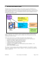
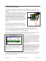
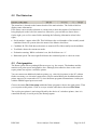
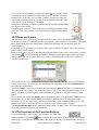
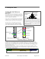
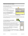
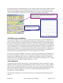
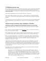
1 The Rotas Noise Analysis System
The Rotas noise analysis system combines a noise analysis program with databases for
parameter settings, archiving and evaluation of measurement data. The core is the RotasPro
analysis application that carries out measurements. RotasPro communicates with the external
test bench control (“PLC”), receives information about the actual test candidate and issues
messages on test analysis results.
Test Bench
Control
(“SPS”)
ROTASDATA
Test Specifications
Database
ROTAS
Measurement
Program
ProductionStatistics
Measurement
Archive and
Presentation
Test
Bench
Further components are the parameter and test specifications database and the statistics
database. Sometimes, there is also an archive available, where measurement curves and
measurement values are stored.
In the scale of this manual, you will find a description of the following items:
o Structural overview of the test bench and the measurement PC, connections etc.
o Operation of the Rotas program, normal test process
o Displays and windows of the measurement program
o Trouble shooting of typical malfunctions and errors
o Installation of software updates, backups
o Definition of new candidate types in the RotasData parameter database (= test
specification database)
o How to use the statistics database
The subject "measurement data archives and their presentation“ is described in a separate
manual. The “parameter database” and the “Statistics”-Tool are described more detailed in
separate manuals also.
DISCOM
Noise Analysis User Manual
Page 5 of 63
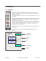
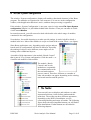
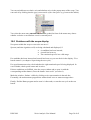
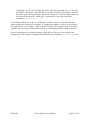
2 Basics of Noise Analysis
The noise analysis uses an acoustic sensor (for structure-borne noise), which captures the
noise signal from a candidate. Additionally, the rotational speed is necessary to carry out the
analysis.
A candidate can consist of several components (e.g. the
inner shafts of a gearbox). Each component contributes to
the total noise read by the sensor. RotasPro can separate
each contribution from the total noise and assigns it to
the different components. The contribution of each
component is being processed separately in synchronous
channels. To separate the signal components, ROTAS
needs the current rotational speed and constructional data
of the candidate. This data is stored in the parameter
database.
For gearboxes, three such rotationally synchronous
signal components are generated and analyzed (labeled
„SK1“, „SK2“, „SK3“). As fourth signal, the total signal
(“Mix”) is also analyzed.
Noise Source
For each of the four signal components, a spectrum is calculated. Some defects leave
characteristically footprints in the spectrum. Additionally, further values (RMS, Crest, see
below) are calculated which allows you to find further defects.
A main noise source is the contact of the teeth of the cogwheels (gear mesh). See the signal
component spectra to clearly identify these mesh frequencies (gear mesh orders).
RMS, Peak and Crest
Peak
Crest
RMS
The RMS value is calculated as the mean energy of the
signal (gear mesh loud = RMS value high). The Crestvalue is calculated as Peak value to mean value
(RMS). A single „Tick“ within a mainly normal signal
produces a high Crest value. Such „Ticks“ are typical
for a defective gear tooth.
For each spectrum, ROTAS provides limit
curves. If a spectrum exceeds the limit curve
in one place, the system takes this position to
identify the kind of defect and issues a corresponding defect message. Likewise, the
single values (Crest etc.) have limit values.
Each candidate type has its own limit values
and limit curves.
Limit curves and limit values can be generated by automatic learning. You can control
and restrict this process through settings in
the parameter database. Only measurements
with an OK result are used for learning.
For each defect you must assign an error
code in the parameter database.
To supervise the production process and the limit values, ROTAS has two statistics databases:
the production statistics and the protocol database. Additionally, measurement data can be
stored in a measurement archive.
DISCOM
Noise Analysis User Manual
Page 6 of 63
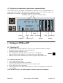
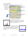
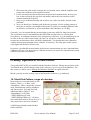
3 The Rotas-PC
3.1 Assembly
The measurement PC is equipped with special signal processor boards
„DPM42“, which process the noise signal and the rotational speed to carry
out the noise analysis.
Depending on the test tasks of the PC, it can be equipped with two or more
such cards.
1
2
DPM 42
3
Different interfaces can be used to communicate with the test bench. At the
moment most of the test benches communicate with the measurement PC
via serial interface (COM2).
Alternatively, a variety of different interface cards can be used, but such
cards are additional equipment of the PC. You can use a Profibus interface
card, for example, and integrate the measurement PC directly into the
Profibus network of the test bench.
Many test benches use also a serial protocol printer. It is connected to port
COM1, then.
The following figure shows how most of the measurements PCs are
equipped:
ROTASPC
serial
seriell
DPM42
DPM42
Communication
Test Bench
Rotational
Speed
Noise
DPM42
DPM42
serial
seriell
Report-Printer
Screen etc.
DISCOM
Noise Analysis User Manual
Page 7 of 63
3.2 Electrical connections (schematic representation)
View of the PC back. The number and alignment of connections can vary depending on the
actual equipment of the PC. The connectors are labelled with a sticker below the connectors.
Furthermore, you find the serial number of the PC on this sticker.
Analogue inputs 1–4 (only 1 is normally used)
LPT2
Mouse
COM1 COM2
USB
Keyboard
(Printer) (PLC)
Rot. speed
Monitor
SCSI
Soundcard
Network
4 Switching the PC ON and OFF
4.1 Start the PC:
1. Open the flap at the front of the PC. (The key can be found in the drawer with the
keyboard or in the folder with the documentation.)
2. Press the ON key for approx. 1 sec...
3. The system starts. The lamps above the ON key (red and green)
glow or flicker. It takes approx. 10 sec until the screen is displayed.
4. If Rotas does not start automatically, start the program as described below.
4.2 Shut down the PC
1.
2.
3.
4.
5.
Close the RotasPro program.
Close all other open programs and windows.
Press the button "Start“ in the left lower corner of the task bar.
Select "Shut down“ from the menu.
A dialog appears. Select “Shut down” and press “OK”. The computer will switch off
automatically.
Never use the ON key or the main computer switch to turn off the computer!!
DISCOM
Noise Analysis User Manual
Page 8 of 63
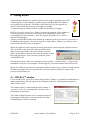
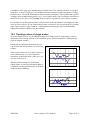
5 Starting ROTAS
On the windows desktop are symbols (links) for the analysis program (grey circle
with red profile), for the database (symbol with yellow D) and for the statistics
tool (symbol with yellow S). The labels of the links can vary, the symbols are
always as described and in shown in the figure (see right).
To start the analysis, double-click the symbol for the analysis program.
ROTAS can not be started twice. Before you start the program, check whether it
is already running (or has not yet been shut down completely). In case you
accidentally have started it twice, “kill” the program by means of Ctrl-Alt-Del
and the Task Manager.
Always wait until ROTAS has been started up completely before you access it, start a test, or
to shut down the program. Please note, that the second window "Stdout“ (see below) sometimes needs some more time to disappear.
While the windows of the program are being opened, the system starts the signal processors.
The two LEDs on the processor cards must show green
light. If the program shows the error message from the
figure on the right on start-up, the system is not able to start
the signal processors. This is a serious problem, please
contact DISCOM.
If the program shows other error messages on start-up (like: „could not find ...“), the current
installation is defective or incomplete. If this happens, you should contact DISCOM as well.
Maybe the LEDs on the processor cards show different colour (red or yellow) or blink instead
of static green light. Don’t worry about this. Our latest software shows the status of the
processor system this way.
5.1 ROTAS 2nd window
If you start ROTAS, you will see that a small window "Stdout“ is opened first and minimized
almost immediately (but will appear in the Windows task bar!). Afterwards the program’s
main window opens.
The Stdout window is linked with the main window: it
can not be closed. It is automatically closed as soon as
the program is shut down.
The Stdout window displays error or status messages of
the program. Furthermore, you can monitor the serial
communication with the test bench.
DISCOM
Noise Analysis User Manual
Page 9 of 63
5.2 The Status bar
The status bar is located on the bottom border of the main window. The fields of this bar
display status information.
If the mouse cursor touches a button or a menu item, a short description of its function is
being displayed on the left of the status bar. Otherwise, you read the text shown above.
On the right, you see five status fields containing the following information (from left to
right):
• Serial number / master-wheel-ID: This field shows the serial number of the actually tested
candidate. Rotas ZP systems show the name of the Master wheel here.
• Candidate-Id: This field shows the name or numerical ID of the actually tested candidate.
• Test Mode: shows the current test mode.
• Evaluation running: While evaluation is on, this field shows an “x”.
• Rotational speed: The most right field shows the rotational speed or a derivate value.
5.3 Print graphics
The Rotas system allows printing different scopes (e.g. the scopes). The database and the
statistics tool print reports and graphics also. Although, this cannot be done on the serial
report printer but requires a windows printer.
You can connect an additional windows printer (e.g. color ink jet printer) to the PC without
further ceremony (see electrical connections). Please remind during the installation that the
printer must not be connected to LPT1, since the Rotas program communicates via this port
with the DPM42 signal processor cards.
Choose the menu File: Print setup within the Rotas program to choose the right printer. Then
you can print to this printer. Click on a scope window and choose the menu File: Print.
The serial report printer is not being affected by the choice of a windows printer, since it is
controlled directly via serial port by the Rotas program.
DISCOM
Noise Analysis User Manual
Page 10 of 63
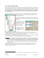
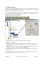
6 ROTAS System Configuration
The window “System configuration“ displays all modules (functional elements) of the Rotas
program. The modules are organized in a tree structure. You can see in the configuration
window, which application function is active, and how data processing is organized.
If the window „System Configuration“ is not open, open it via the menu File: Open System
configuration. Maybe it is just hidden behind other windows. Then you can make it visible
via the menu Window.
In normal test mode, you will not need to deal with details or the whole range of modules
contained in the configuration.
Nevertheless, for trouble shooting or to make special settings, it can be helpful to check a
module in the tree. Most of the modules in scope are listed in the section “Host“, (see figure).
Since Rotas applications vary, depending on the project and test
bench used, its configurations will also be different. Especially
the ranking of objects can be different, some might even be
lacking or have additional objects.
A module of high importance is the module “Bench Control”
that is part of every system configuration. Click the small +, to
visualize sub-modules of this module.
The module „Bench
Control“ and its submodules are responsible
for communication with
the test bench and test
process control. Therefore, different or a number of
other sub-modules can appear depending on the existing
test bench interface and the process.
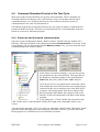
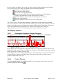
7 The Toolbar
You can easily access displays and windows or other
important functions via the toolbar (underneath the
menu bar). The toolbar can have different appearance,
depending on the ROTAS installation you use,
concerning labelling and range of buttons. The following
figure shows the most important buttons you will find in
most installations. Further buttons are described in
following chapters.
DISCOM
Noise Analysis User Manual
Page 11 of 63
Test condition,
see ch.9
Rotational
Speed display,
see ch.9
Scopes:
Spectra, Time
Signal,
see ch.10
Report Window,
see ch.11
Traffic light,
see below
Table window
see ch.11
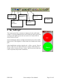
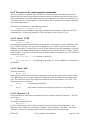
8 The „Traffic light“
The actual result of the evaluation is displayed in the traffic light
window. It is being updated at the end of each test mode (gear test):
As long as the light is green, the test result is ok. It turns red if a
defect has been found.
red
Some installations display red light in the bottom area of the traffic
lights as well. This happens if a defect has been found in the actual
gear.
Other installations use three signals (red – yellow – green). Green is
shown, if the test is ok. Red is shown if a “major” defect has been
found, yellow is shown if only a “minor” defect has been fond (test
can be repeated, maybe after refinement).
DISCOM
Noise Analysis User Manual
Green
Page 12 of 63
9 Supervising the test cycle
In the Rotas system, each Step of a test (different gears, separated in speed going up and
speed going down) is defined as a test mode. Indicated by the external test bench control
(PLC), these test modes are accepted and evaluations are being made. But, first of all, the test
bench control has to inform Rotas, which type of candidate is being tested, preparing Rotas to
calculate the right frequencies of the cogwheels.
9.1 Test Status
The display "Test Status“ shows how the automatic noise analysis is being processed. Use the
toolbar button
to open the dialog.
Please note, that the operating mode is „Controlled by Bench
control“.
The list box displays the type of the currently tested candidate (type
„1“ in the example).
If the candidate is within the test bench, Ready will be marked
(appears pushed).
You can watch in the list, how the different test modes are selected.
During the noise analysis, the field Measure will be marked (pushed).
As soon as the mark disappears, evaluation has been done and the
result is issued.
If the right type of candidate is not displayed or the modes are not
being selected, although the operating mode is “Bench control”, check
the connection to the test bench (PLC). Please note that you have to
change to operating mode “Bench control” before the test bench
inserts the candidate.
You can change to a smaller version of this dialog by pressing the small
button Ø below the close button x:
This display shows current type and current test mode as well.
9.2 Rotational Speed Display
The display instrument "Rev. Speed“ views the current rotational speed. Additionally, the
rotational speed is displayed in the status bar of the program (lower
edge of the window).
If you do not receive any rotational speed, check the speed sensor
on the test bench and the connection to the ROTAS-PC. Without
rotational speed information, no spectra will be displayed!
DISCOM
Noise Analysis User Manual
Page 13 of 63
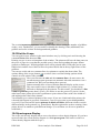
9.3 Start- and Stop values
Many test benches control the noise analysis via so called Start and stop values.1. That means
that an analogue signal is taken as control value for starting / stopping the analysis. In general,
this analogue signal value is the current rotational speed from the test bench. The range for the
acoustic analysis in a certain test mode has been preset in the Rotas system. For example, it
can have been preset that the acoustic analysis in the 3rd gear speed up starts at 1200 Rpm and
stops at 3500 Rpm.
Start/Stop rotational speeds for different test modes and candidate types are defined in the
database. You can easily view them in the program and enter
(temporary) changes.
Open the system configuration and double click on the module
“Trigger Decoder” (picture or name). The trigger decoder dialog
will appear:
This dialog lists the speed
ranges of all test modes.
Select a line, to view the
interval in the entry
fields, on the right.
Enter a new interval for
the selected gear, and
click Apply, to activate it.
If trigger ranges are defined in the database, the new interval is valid only until the next
update from the database. Usually, an update is being done when a new candidate is inserted.
Lasting modifications must be entered in the database, then.
Some test benches use different analogue signals to start/ stop the test (e.g. start on speed, stop
on timer). Then you find different trigger decoders for each control signal.
Please note: For accurate test results, speed up and speed down test runs must not be done too
quickly. Per 400 Rpm rotational speed change, at least 1 sec must be counted. Example:
For a speed up run of 1200 to 2400 Rpm, the range of 3 x 400 Rpm is crossed, and must
not last less than 3 sec. To guarantee safe process control, the rotational speed limits
must have some 100 Rpm distance from the actual switch-over rotational speed values
of the test bench.
Furthermore, please note that the trigger values have to fit the speed ranges from the test
bench. During a ramp the speed range defined in the trigger-dialog has to be measured
completely by the test bench.
1
Other test benches transmit commands for start and end of the noise analysis directly. If so, please ignore this
chapter.
DISCOM
Noise Analysis User Manual
Page 14 of 63
9.4
Command Orientated Control of the Test Cycle
Most test benches control the Rotas test system with commands. These commands are
normally transferred to Rotas via the serial interface. Some test benches transfer these
commands directly via a Profibus interface card. Nevertheless, the basic system of
communication is the same for both interfaces.
If the Rotas program shows unexpected behaviour, the reason is mostly a communication
problem with the test bench. Therefore you should check first, if all commands of the test
bench are received by the Rotas program.
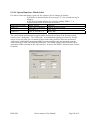
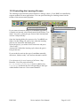
9.4.1 Supervise and test serial communication
Open the system configuration and the “Bench Control“. Double-click the module “PLC
Interface“ (having a telephone icon) and press the button Characteristics in the dialog. In the
second dialog, you can activate the function Monitor Comm. Now, you can watch the serial
communication in the window Stdout.
In the dialog “Serial Port Settings”, you can also specify
the parameters for the serial interface. The figure shows
the Windows’ standard settings for the serial interface:
9600 Baud, No parity, 8 bits of data, and 1 Stop bit.
If you do not receive any data from the test bench, check
first whether the serial cable from the test bench has been
connected to the correct interface port of the ROTAS PC
(compare with settings made in the above dialog of the
Rotas program!) and whether the settings for the serial
interface of the test bench match with those of the Rotas
program.
Is everything ok? – Check whether the test bench sends
CR/LF at the end of each commando. Maybe the length of the commando buffer is not
correct.
You can use the input line “Test” (see above) to “distribute” data by hand. The button “Send”
sends the data in the input line to the test bench, the button “Receive” gives the data to the
Rotas program, as if it had been received from the test bench.
DISCOM
Noise Analysis User Manual
Page 15 of 63
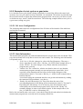
9.4.2 Overview of the most important commands
There are multiple commands with which the test bench can control the Rotas test system,
enquire data from the Rotas program and transfer data to the Rotas program. For this reason,
the used commands can differ significantly between different test benches. Nevertheless, you
will find a basic set of commands on all test benches. These commands are shortly explained
in the following chapters.
Basically, all commands use the following format:
Command: Argument CR LF
A colon follows each command, separating command and arguments. At the end of EACH
command line, a Carriage-Return and a Line Feed must be sent (ASCII 13, 10).
9.4.2.1 Insert: TYPE
With the command
Insert: TYPE
the test bench informs the measurement program that a new test cycle with a candidate of the
type “TYPE” shall start. The type (the test instruction set) “TYPE” must be defined in the
database. Otherwise it is impossible to test it. When Rotas receives this command, it reads the
candidate specific data from the database and prepares itself for the test. The “Ready” button
in the window “Test State” reflects this fact by being displayed in pushed state. The test bench
receives the answer:
<R>Inserted: 1 , if everything worked fine,
or
<R>Inserted: 0 , if something went wrong, e.g. if the candidate is not defined in
the database.
9.4.2.2 Mode: ABC
With the command
Mode: ABC
the test bench informs the measurement program which test step (gear/ramp) shall be tested
next. When Rotas receives this command, it adapts its analysis parameters according to the
gear. The actual test step will be displayed in marked state in the window “Test state”. The
test bench receives the answer:
Ready
, if everything worked fine,
or
Mode?
, if the mode command was unexpected or the test step unknown.
9.4.2.3 Measure: 1/0
Some test benches control the measurement directly with the command “Measure”. The test
bench issues
Measure: 1
to start the measurement and
Measure: 0
to end it. When Rotas receives this command, all received data between Measure: 1 and
Measure: 0 are evaluated to classify the candidate. In the windows “Test State”, the button
“Measure” reflects the running measurement by being displayed in pushed state.
DISCOM
Noise Analysis User Manual
Page 16 of 63
This command is not answered by the measurement program, but there exist answered
variants of this command (see appendix).
If the measurement program itself controls the measurement with Trigger values (see above),
the test bench must not send this command.
9.4.2.4 Remove:
With the command
Remove:
the test bench ends a regular test cycle. The measurement program will react by storing all
cumulated evaluation values and sends the test result to the test bench with the answer:
<R>Result: 1
(Candidate o.k.)
or
<R>Result: 0
(Candidate n.o.k.)
The button “Ready” in the window “Test state” will no longer be displayed in pushed state.
9.4.2.5 Reset:
The Command
Reset:
ends a test cycle without Rotas storing its evaluation data. It is used to get Rotas in a defined
state after a failure (“Initial position”). It is answered with the line:
<R>Status: Reset
Many test benches send, before issuing the Insert-command, a Reset-command to ensure that
Rotas is in initial state.
9.4.2.6 RequestStatus:
With the command
RequestStatus:
the test bench can enquire whether the measurement program is capable of processing
commands from the test bench at that moment. It is answered with
<R>Status: Online
if the measurement program is currently capable of processing test bench commands.
Except on startup (when initializing the program), there is only one possibility why the
measurement program is unable to process test bench commands: In the window “Test state”
the mode “Manual” has been selected. Thus, the answer is
<R>Status: Handcontrol
when Rotas can not process test bench commands at that moment.
DISCOM
Noise Analysis User Manual
Page 17 of 63
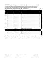
9.4.3 Example of a command sequence
The following table shows an example of how a complete test cycle of a four-gear gearbox
can be controlled by the test bench. The measurement itself is controlled by trigger values.
Command from test bench
Answer from Rotas
RequestStatus:
<R>Status: Online
Reset:
<R>Status: Reset
Insert: 4711
<R>Inserted: 1
Mode: R-Z
Ready
Mode: R-S
Ready
Mode: 4.Z
Ready
Mode: 4-S
Ready
Mode: 3-Z
Ready
Mode: 3-S
Ready
Mode: 2-Z
Ready
Mode: 2-S
Ready
Mode: 1-Z
Ready
Mode: 1-S
Ready
Remove:
<R>Result: 1
DISCOM
Noise Analysis User Manual
Page 18 of 63
9.5
Bit-orientated control of a test cycle
Some test benches (e.g. the gear testers) communicate not (or not only) with the Rotas
program using control commands, but use “control bits”. These control bits are transferred to
the measurement program either via digital I/O cards or directly via a Profibus interface card.
You can supervise these communication lines in the Rotas program as well.
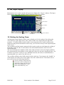
9.5.1 The “Main Window” of the Parallel Control Unit
Open the system configuration, and then go to “MeasureCourseControl Container”. Doubleclick on the module Command-Decoder (or “Bit-Decoder”). Two windows will be opened.
One of them is this one:
In this window (referenced as mainwindow in the following text), you
can supervise all the I/O lines as
whole bytes (characters).
Furthermore, there are different
options.
The left side of the window shows
the input lines, the right side shows
the output lines.
You choose with the settings "from"
and "to" which interval of the I/O
lines are being displayed. About 16
Lines fit into the window.
The first byte of the input/output area
respectively has number 1.
In addition to that you can have a
byte 0. This is not a real output address, but a “dummy address” for internal use of the
control program.
In the figure, the input-area is displayed in „Byte-View“, the output-area is displayed in
„function-view“.
The Byte view shows one byte with its actual value as number and character in one row. You
use it to supervise whole bytes directly.
The function view shows one function with its actual value in one row. The last line of the
output list displays, that Byte 3, Bit 4 with Function “Life” has the value 1. In the function
view you see the data in the decoder’s interpretation. If a test bench sets 10 characters
consecutively (maybe a serial number) these characters are being displayed as one string. You
need not supervise 10 single bytes.
In the function view you only see bits/ bytes/ areas which have an actual function. Bits/ bytes/
areas which have several functions are being displayed once for every function. In the figure
above output bit 2.3 has the functions “Insert.Result” and “Result”.
To be able to verify data in the function view, you must know how the decoder reads the data.
Often, a function is only valid under certain circumstances. (A ten byte string can be typeinformation if bit “Type” is set or serial information if bit “Serial” is set.)
DISCOM
Noise Analysis User Manual
Page 19 of 63
9.5.2 Supervising and manipulating single bits
A single click on an entry in the first column of the table (in/out
respectively) opens another window in which you can supervise
and change the state of single bits (referenced as “bit windows” in
the following text). The bits in these windows are ordered as
follows: Bit 7 is the topmost bit; Bit 0 is at the bottom.
If you click on a check-box in one of the bit-windows, the value of
this bit is directly changed. If this bit is an input bit, the actual data
from the I/O card will overwrite this change in most cases. In case
of an output bit the change is written to the I/O card directly
(except for status-bits, which are being refreshed from the control program frequently).
The labelling of the bits in a bit-window is dependent on the settings made in the main
window. “In_3” is labelled in byte-view and shows the names of the bits. “Out_3” is labelled
in function view and shows one function of the bit. (If a bit has more than one function, only
one function is being displayed). You may notice, that bit 1 (between Busy and Inserted) has
not been labelled, although it has a function. The reason is that the functional dependency is
different for this bit.
9.5.3 Manipulating functional values
As mentioned above, the function view is used to display values in the form as the decoder
reads them. Sometimes you want to manipulate these values (e.g. a serial number), without
having to manipulate single bits in several windows. For this reason, a window exists which is
used universally to manipulate functional values, consisting not necessarily of single bits. The
bit 1 of “Out_3” which has been mentioned above is such a value. If you click on the entry 3.1
in the main window, you see the following window:
This window always displays the actual value on the I/O card in the moment, when you
opened the window. If you enter a value and click “Apply”, this value is written to the I/O
card (same exceptions like the bit windows).
How the value is formatted and which interval is valid depends on the processing module. In
the example shown above, it is a single bit (to be more exact: a number between 0 and 1).
Under other circumstances it can be a number between 0 and 65565 or a string.
Sometimes you prefer one view to the other. If you want to check the state of single bits on
the I/O card, you choose the byte view and additional bit-windows. If you want to check how
Rotas reads the data from the I/O card, you choose the function view and watch the entries in
the main window.
DISCOM
Noise Analysis User Manual
Page 20 of 63
9.5.4 Simulation and monitor mode
You can choose "simulation" in the main window and test functions manually. In this mode,
no values are being read or written from/to the I/O cardDon’t forget to switch back to "normal" after you finished your tests in "simulation" mode.
To supervise the processing of the bits, you can activate the “monitor” function. When you
activate one of these check boxes, you get a report written to the Stdout window for each
value change in every open bit window (In_3, e.g.):
All value changes which Rotas notices
simultaneously are listed with the name of
the bits. In addition to that, the new value of
the whole byte is reported at last. A “short”
line separates this byte’s data from next
byte’s data.
At the end, a "long" separator line finishes
the list. The reported changes between one
long separator line and the next have been
noticed simultaneously by the Rotas
program.
Manual changes in the bit windows are not
being reported.
DISCOM
Noise Analysis User Manual
Page 21 of 63
9.5.5 Example of a test cycle on a gear tester
It is clear that a test cycle which is being controlled via control bits follows the same basic
structure as a test cycle which is being controlled via commands. This means in particular that
the test bench needs to inform the measurement program when a new test cycle starts as well
as which test step (“mode”) shall be tested next. The following example shows a test cycle of
a gear tester (testing one gear).
9.5.5.1 I/O Area Configuration
The following tables show the configuration of the I/O lines of the interface. Bits which are
not labelled are unused.
Input lines:
Bits
0
1
2
3
4
5
6
7
In_1
INSRT MDSET
DIR
RMV
TTHGT
In_5
Type as Byte values
Output lines:
Bits
0
1
2
3
4
5
6
7
Out_1
LIFE
ONL
INS
RDY
MEAS
RVD
Out_2
IO
NIO
FAL
Out_3
EINSRT EMDSET
ETTHGT
Out_5
TH1 (defective tooth 1)
9.5.5.2 State Information
The measurement program can send information about its current state to the test bench. That
way, the test bench can verify that a correct test can be made. The following state information
is frequently used:
o “Life“-bit. A “life-bit“ changes its value with fixed frequency. That way a
device signs that it is still „alive“. Bit Out_1.0 (LIFE) in the example above is
such a “life-bit”. Its value changes every 500ms when the measurement
program runs correctly.
o “Online“-bit. The “online-bit“ tells the test bench (when it is set) that the
measurement program currently accepts and processes control bits. It is 0
especially when manual mode has been selected in the dialogues of the
measurement control (“Test state“). Bit Out_1.1 (ONL) in the example above
has this function.
A test bench using the command interface can get this information by sending
the command „RequestStatus“ (see above).
o “Ready“-bit and “Measuring“-bit. These bits show the state of the
corresponding buttons in the dialog of the measurement control (“Test state”).
Especially the “Measuring“- bit is of interest, since this function can be
controlled by the measurement program itself, whereas the “Ready”-bit
normally changes its state on test bench request. In the example above, bit
Out_1.6 (MEAS) is such a “Measuring“-bit.
Before the test bench starts a test cycle, it can check using life-bit and online-bit whether the
measurement program runs correctly and is accepting control bits.
DISCOM
Noise Analysis User Manual
Page 22 of 63
9.5.5.3 Example of a sequence of control bits
A general fact is that a value change initiates an action. For this reason, the NEW value of a
bit is given in the following example. The function explanation includes (as far as possible)
the command of the command interface having a similar function.
Data from test bench
Type: 1
INSRT: 1
Rotas’ answer
INS: 1
EINSRT: 1
DIR: 0
MDSET: 1
MDSET: 0
RDY: 1
EMDSET: 1
EMDSET: 0
MEAS: 1
IO: 1
MEAS: 0
DIR: 1
MDSET: 1
MDSET: 0
RMV: 1
INSRT: 0
RMV: 0
RDY: 1
EMDSET: 1
EMDSET: 0
MEAS: 1
IO: 1
MEAS: 0
INS: 0
RVD: 1
EINSRT: 0
RVD: 0
Function
“Insert: 1“: Starting test cycle, type „1“
1: Everything ok, 0: Error, e.g. unknown type
INS-Bit valid
“Z“ (Direction “Z”)
“Mode: Z“: activating test step „Z
1: ok, 0: Error
RDY-bit valid
Reset bits
Rotas started the measurement
IO, NIO, FAL depending on evaluation current mode
Rotas stopped measurement, evaluation result valid
“S” (Direction “S”)
“Mode: S“: activating test step “S
1: ok, 0: Error
RDY-bit valid
Reset bits
Rotas started the measurement
IO, NIO, FAL depending on evaluation current mode
Rotas stopped measurement, evaluation result valid
“Remove“: End test cycle.
Rotas completed test cycle
Reset bits, “Reset“
Reset bits
The function “Reset” in the last but one line is equivalent to the “Reset” command. That
means, if the bit INSRT gets the value 0, without bit RMV having set to 1 before, the
measurement program stops the test cycle without storing data (abort).
DISCOM
Noise Analysis User Manual
Page 23 of 63
9.5.5.4 Special function: Mark defect
If a defect is detected during a gear test, the sequence above changes as follows:
- if the defect is detected in the first test step (“Z”), the second test step is
skipped
- before the test bench ends the test cycle by sending “RMV: 1”, it
enquires the position of the defect as follows:
Data from test bench
Rotas’ answer
Function
TTHGT: 1
TH1 value of position
Enquire defective tooth
ETTHGT: 1
TH1 valid
TTHGT: 0
TH1: 0, ETTHGT: 0
Reset data
The value that the measurement program sends, defines the position of the defective tooth
relative to the “Null pulse”. The “Null pulse” is an additional signal given to the PC for this
reason. It has one pulse per revolution (always at the same position). Since the position of
“Null pulse” and marking instrument differ between machines, the measurement program
allows entering a value correcting this difference. The setting dialog for this function can be
opened by double-clicking on the “Sps-Decoder” in the section HOST->Measurement Control
Container.
DISCOM
Noise Analysis User Manual
Page 24 of 63
10 The ‚Scope’-Displays
Measurement curves (time signals) and spectra are displayed in “Scope” windows. The figure
below shows some of the essential control elements of the scope window:
Y-unit
Data area
Y-Axis
Y-Scroll bar
Zero-Mark
Labels
x-Axis
x-Scroll bar
Control buttons
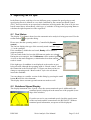
10.1 Setting the Scaling, Zoom
An important control function of the scope as display tool is the setting of the scaling (the
value interval). In the figure above, the x-values of the curve range between 0 and 0.023
seconds (= 23 milliseconds), but the visible cut-out ranges between 2 and 16 milliseconds.
With the scaling and zoom function of the scope, you can focus closely on the important parts
of the curves.
The scroll bars and the buttons connected with it can be used to set and change the scaling of
the display. Each axis has its own buttons, but similar labelled buttons on the axes have
similar functions.
The axis itself shows the smallest visible value at the left end (2.0 ms in the figure) and then
the values marled by the gridlines. At the right end of the axis, the unit is displayed (here s for
seconds). If you have very big or very small data intervals, the values are transformed to a
usual unit milli- (m), .micro- (µ), kilo- (k), etc.
The scroll bar influences the visible interval in the usual way. You can move the “handle” or
click into the area to the left of to the right to move the visible interval. The buttons next to
the scroll bar have the following functions:
Zoom in (enlarge scaling interval)
Zoom out (reduce scaling interval)
Automatic scaling (this axis only)
Set 0 at the beginning of x-axis
Set 0 at the bottom of y axis
DISCOM
Noise Analysis User Manual
Page 25 of 63
If you zoom into the data by pressing the button , the „handle“ of the
scroll bar becomes smaller to indicate that you see a smaller cut-out of
the data now. If the size of a scroll bar "handle" is incorrect (after the
start of the program), click on a zoom or arrow button at the end of the
scroll bar to get the scaling re-calculated.
Sometimes, zooming sets the zero position beside regular scaling marks
(see figure on the right).
If this happens, you can “correct” the axis by clicking the handle of the
scroll bar. The zero position is moved to the next regular scaling mark
by that.
10.2 Panes and Labels
The data area can be split in several panes and the curves can be assigned to different panes.
(In a spectra scope of a standard gear box test system, you normally see four panes. The upper
three panes show the noise components of the different shafts, the fourth pane show the
overall signal.)
If the data area is split into several panes, the x axis is valid for all panes. The y axis of each
pane is labelled individually.
Right of each pane, you see a label box showing the names of the curves in the curve’s colour.
(you find it among the function buttons in the bottom right corner) opens the
The button
dialog where you can set panes and curve colours. This dialog shows all curves, which are
“known” to the scope:
The list shows the curve’s names, their current colour and the pane where they are displayed.
If you select a curve in of the list, you can change the properties in the frame Darstellung on
the right side of the dialog.
Select the colour for the curve from the list and select the pane where the curve shall appear.
The pane at the top is pane 1, the next pane below is No. 2, etc. The maximum number is 12
panes. All panes up to the highest selected number are painted, even if this contains empty
panes.
If you disable the check box display, the corresponding curve is being hidden. Hidden curves
do not have an x in the column Show. Nevertheless, hidden curves are displayed within
brackets (“{}”) in the list of curve labels to indicate that a pane contains hidden curves. All
hidden curves are re-activated when you close the scope window and re-open it.
The Zeichen-Reihenfolge allows influencing which curve is painted last. This curve appears in
the foreground and is listed on top of the list.
10.3 The Functions of the Function Buttons
In the bottom right corner of the scope window, you find eight
function buttons. The button
shows or hides the curve labels. If you hide the curve labels
more space is available fort he data panes. The button is displayed in pushed state as long as
DISCOM
Noise Analysis User Manual
Page 26 of 63
the curve labels are enabled. If you hide the labels, the four leftmost buttons also disappear
(for special reasons). The other four buttons have the following functions:
Automatic scaling (both axes)
Store current scaling settings
Re-activate stored scaling settings
Freeze the curves: The curves are not refreshed any more. This button is
displayed in pushed state as long as the curves are frozen.
Opens the dialog to set the curve colours and panes (see above).
Opens the options dialog
Opens the window where you can focus on data points
The “Freeze curves“ function allows making a “photograph“ of the current measurement
curves. You can have a closer look at the curves then (e.g. zoom at points of interest, read out
values or print the curves), while the measurement continues in the background. If the scope
is part of a regular analysis application (e.g. transfer case analysis), the scopes are
automatically "un-frozen" at certain points of the automatic measurement cycle.
10.4 Display Options
10.4.1
Rectangular Display or Display Polygons
You can choose between two forms of the curve display: As polygons or rectangular:
mV
mV
links
links
4.0
4.0
3.2
3.2
2.4
2.4
1.6
1.6
0.8
0.8
0.0
0
0
200
400
600
800
1000
1200
1400
1600
1800
Display as Polygons
Hz
0.0
0
200
400
600
800
1000
1200
1400
1600
1800
Hz
Rectangular display
If you display curves as polygons, each point of the curve is directly connected with the next
point. Thus, each “corner” of a curve stands for a data point. This display form allows reading
out the x-position of a data point very well.
If you display curves in a rectangular display, for each data point gets a horizontal line which
is centred at the x-position of the data point. This display form allows reading out the yposition of data points very well.
10.4.2
Further Options
The dialog Scope-options allows adjusting different visualization options of the scope. You
open the dialog with the button .
DISCOM
Noise Analysis User Manual
Page 27 of 63
The section Darstellungsoptionen in the top left corner allows setting the number of gridlines
on the y-axis. Furthermore, you can enable or disable the drawing of the (additional) zero
gridline and set the colours for background and gridlines.
10.5 Print the Scope
You can print a scope window in the usual windows way by clicking on it and choosing the
command Print from the menu File.
Printing a scope is not a real snapshot of the window. The printout will have the data panes on
the piece of paper in a way that the possible space is best used regarding the paper format
(portrait or landscape). No background colour will be printed either. Each pane gets its own
labelled axis and the curve labels will not be printed beside but in the top right corner of the
gridlines.
You can use a title and two comment lines in a printout to explain the shown data. The
options dialog of the scope (button ; see above) has a section Printing options which
controls several options if the printout:
Here you can enter the title and the comment lines. (In most cases, the
measurement program generates an automatic title and sometimes even a
comment line. But you can change these presets.)
Printers naturally have a finer resolution than the display on the screen.
This can result in curves which have light colours (e.g. yellow) being
difficult to distinguish in the printout. For this reason, you should set a line
width for printout greater than 1 (pixel). (We advise to use the preset of 2 pixels.) On the
other hand, some printer drivers have problems to print coloured lines with a line width of 1
and might produce black lines instead.
You normally get a coloured printout of the scope. If you use a black and white printer, the
coloured lines appear in greyscale. Sometimes, curves in greyscale are not distinguishable
very well. If you activate the option printout in black and white, different colours result in
different linings in the printout (e.g. dotted lines). But this option also needs a warning: Some
printer drivers are unable to print different linings. (You will then see all curves printed in
solid black.)
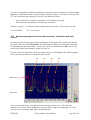
10.6 Spectrogram-Display
The scope can not only display data as curves but also as colour density diagram. (If you have
spectra as data, the colour density diagram is called spectrogram. This name is used for a
colour density diagram with the scope.)
DISCOM
Noise Analysis User Manual
Page 28 of 63
In a spectrogram, each curve is transformed into a coloured pixel line of the image. The
colour of a pixel depends on the value of the curve at this point. You normally use lighter and
more intensive colours for high values:
When the scope receives a new curve, the current image is moved by one pixel line to the top
so that the image data of the older curves remain. Thus, the spectrogram display allows
getting an overview about the nearest past. On the other hand, you can not read out the values
as exactly as with the normal curve display.
You activate and deactivate the spectrogram display via the context menu of a data pane. You
click with the right mouse button into the pane and choose the topmost command
spectrogram:
In a spectrogram display the data values are transformed into colour values. A colour map
with a defined number of entries is used for this transformation. This colour map is used in a
way that it covers the currently visible interval of the y-axis. If you change the range of the yaxis by zooming or moving, the colours transformation of the spectrogram will change either
(but you will see the change only with new curves). If you use the button to adjust the
scaling of the y-axis automatically, the colour transformation is adjusted either to cover the
range of the y-axis.
The x-axis is set for all curve plots and spectrograms at the same time (as long as the
spectrogram runs „vertically“, see the spectrogram options below for details). If you change
the scaling for the x-axis by zooming or moving, the spectrogram will change as well (only
for new curves either).
10.7 Relative and Absolute Scaling of the x-Axis
Some curve data, especially the order spectra of a transfer case analysis can be displayed
using two different scaling factors. These scaling factors define the relations between the
spectra of different shafts at different speed.
The two scaling factors you can use are as follows: If you use relative scaling the x-axis of the
spectra in the scope refers to the speed of the shaft. If you use absolute scaling, the x-axis of
the spectra in the scope refers to the speed of the speed source.
In other words, if you see a peak in the scope, you see the frequency (order) of that peak on
the x-axis if you use “relative scaling”. If you use “absolute scaling”, you see the frequency
(order) of the speed source (input shaft) at the position of the peak.
This difference results also in a different length of the curves. With an “absolute axis”, the
relative rotation frequency assigns the length of the curves (shafts which rotate with a smaller
frequency produce shorter spectra). With a “relative axis”, the length of the curves is the real
length of the spectra (in general a power of 2).
DISCOM
Noise Analysis User Manual
Page 29 of 63
You can switch between relative axis and absolute axis via the popup menu of the scope. You
can reach it by clicking into the (grey) area outside of the data panes (e.g. between the labels):
You select the menu entry absolute x-Achse. The symbol in front of the menu entry shows
whether a relative or an absolute x-axis is currently used.
10.8 Problems with the scope display
No spectra within the scope or curves do not move?
Spectra (and time signals as well) are being calculated and displayed, if
• A candidate has been inserted,
• A mode has been set,
• The rotational speed is in a valid range.
If a candidate has been inserted and a mode has been set, you can check in the display “Test
bench control“ (see chapter: Supervising the test cycle).
If a speed instrument exists, check whether the right rotational speed is being displayed. In
case of doubt, check speed sensor and its wires.
If these conditions are fulfilled, close the scope window and re-open it (with the
corresponding toolbar button). Press the button “Auto scale” (see above).
Make the window „Stdout“ visible by clicking on its representation in the task bar.
Eventually, the measurement program has written down error or status messages there.
Finally: End the Rotas program and re start it. Afterwards, re-start the test cycle at the test
bench.
DISCOM
Noise Analysis User Manual
Page 30 of 63
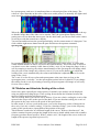
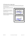
10.9 Tracking values of single orders
Some test benches carry out an additional analysis of single spectral components („orders“,
sometimes mesh orders) relative to the rotational speed. This measurement is displayed in a
separate display window.
During the up and down measurement, you
can see how the measurement curve is being
written.
Track_H1 in SK1, Z
dBmm/s
80
There can be limit curves for these curves as
well. Alternatively you can evaluate the
maximum or the mean value of the curve (or
of parts of the curve).
70
60
50
40
Whether such an analysis is performed,
which orders are involved and which kind of
evaluation is being performed, this is defined
in the parameter database.
30
20
0
500
1000
1500
0
500
1000
1500
2000
2500
3000
3500
4000
4500
2000
2500
3000
3500
4000
4500
Track_H1 in SK1, S
dBmm/s
80
70
60
50
40
30
DISCOM
Noise Analysis User Manual
Page 31 of 63
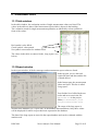
11 Measurement results
11.1 Table window
In the table window, the evaluation results of single measurement values are listed. The
values in the table are those if the last measured gear which is shown in the heading.
The evaluation result for single measurement quantities are labelled by colour symbols in
front of the values:
Red symbol: value failed
Green symbol: value passed
No symbol: not measured or without result
The values in the table are entered in the „long report“ (see
below.)
11.2 Report window
In the report window, all defect messages and measurement report values are listed.
In the top part, you see the total
result with time and date and the list
of found defects.
In the bottom part, the measurement
values are listed. This list is called
“long report”.
You find the list of all defined error
codes and error texts in the file
Errorcode.set in the project
folder (C:\RotasData\(Your
project)\Errorcode.set).
The range of the long report is
defined in the database (see "report lists" in the database documentation). Only those values
will be displayed for which a report has been requested in the database.
The data of the long report are stored in the report database and can be evaluated with the
statistics tool.
DISCOM
Noise Analysis User Manual
Page 32 of 63
11.3 Report printing
All data which is displayed in the Report window (defect report/ long report) can be sent to a
serially connected report printer (with endless paper). You can set the amount of data in the
printed (stored) report in a dialog of the program.
Open the dialog, using the button in the toolbar. If your project’s toolbar does not show this
button, you can reach the dialog via the system configuration as well. Right click on the
symbol “Print report” and choose Options….
In the dialog, select the sheet „Output line“:
In the dialog, choose between the following options for report printout:
•
•
•
•
None: no report is printed.
Short: for OK tests, only the serial or palette numbers are printed on one print line
(Therefore, the length of a print line can be set in the field.) For NOK tests, the defect
report is printed.
Normal: for each test, a full line is printed, indicating type, serial number, test time, total
result etc. For NOK tests, the defects are listed additionally.
Long: see ‚normal‘, but the „long report“ containing the measured values is printed
additionally.
„Output in manual mode“: normally, printout is done in automatic mode only. Use this
checkbox to print reports when Rotas is in manual mode, too.
DISCOM
Noise Analysis User Manual
Page 33 of 63
"Bench controlled“: Some test benches have a button directly at the test bench to indicate that
a long report is required. This button gets activated by this checkbox.
„Form feed for defect reports“: If this option is active, a form feed (page break) is generated
after and before a NOK test. This will have the effect that the defect report of a candidate is
printed on a separate page.
Print a Line: Press this button to print a horizontally dotted line. Use it to mark printouts or to
test the printer.
11.4 Request One-Time Long Report.
You might have the situation that you want to have a long report printout only for the
currently tested candidate (like a calibration type or a prototype). This function can be
activated via a button in the toolbar.
Press the indicated button using the mouse. Doing so will request a long report for the current
test (or the directly following test). The protocol is printed at the end of the complete test.
The button stays pressed until the report has been printed and
indicates that a long report has been requested. If you release
the button before the end of the test run using the mouse
(press again), you cancel the request and the program prints as
preset in the dialog (see previous page).
DISCOM
Noise Analysis User Manual
Page 34 of 63
11.5 Storing Measurements in an Archive
In some installations, you can configure Rotas in a way that all measurements (curves,
evaluated spectra, protocol values etc.) are stored in archive files.
You can evaluate these archive files with the presentation program later.
Find the module “Store measurements” in the system configuration to activate archive
storage. You find this module in the section “Host”:
Double click this module to get the settings dialog:
Verify that the check-box
Write files has been checked if
you want to store
measurements in an archive.
Furthermore, you set in this
dialog in which folder the
measurements are stored.
Normally one file is generated
for each measurement (each
gear box).
If you check enumerated files, the filenames are generated using the entered base name and
the counter. Otherwise, the actual serial number (transmitted from the test bench) is used
instead of the counter.
In the system configuration, you find directly below the „Store measurements“ a module
„Concat files“. This module is able to
merge single files (single measurements)
to larger files. Double-click on “Concat
files” to choose how the measurements
shall be sorted.
Verify again that the check-box
Concatenation is active has been
checked if you want the module to
concat single files.
You can choose between different sorting methods. Consider that the
archive files will pile up on the hard disk. Depending on the amount
of the test, a single measurement archive can have the size of 50-150 Kbytes. If you let a test
bench store archives for some weeks, the hard disk will be full one day.
Two strategies exist against this: You can copy the data to a server (and burn it on a CD if you
wish), or you can select the sorting option week days. If you do so, the measurements of one
weekday are stored in one file (you will get a Monday-file, a Tuesday-file etc). After one
week, the old file is deleted and a new one is created. That way you have all the measurements of the previous week at hand without having an unlimited need for storage capacity.
DISCOM
Noise Analysis User Manual
Page 35 of 63
12 Measurement type definitions
This chapter describes how the most frequently used measurement types are calculated and
what they tell about a candidate, especially a gear in a gear test. With a gear box, the
measurement types refer to the gears of one shaft.
12.1
Measurement types from the time signal
Null-pulse
Smoothed Signal
Signal
The figure above shows the time signal of a
cogwheel with one defective tooth. Such a defect
leads to a ticking noise in a gear test and in an
assembled gear box. The figure on the right shows
the table of measurements with the values
calculated from this signal.
Three different measurement types are calculated
from the time signal: Peak, RMS and crest.
The peak is defined as the maximum amplitude of
the signal. It is read directly from the time signal or the smoothed signal. A high peak value
results when the cogwheel has a defective tooth with a nick.
The RMS value reflects the energy contained in the signal. The mean value of the smoothed
signal tends to mirror the RMS value (as you probably can imagine). In other words: The
RMS value is high when you have many peaks on the signal. On the other hand, one isolated
peak (see above) does not lead to a high RMS value, since its effect is negated by the
predominance of the signal’s lower parts. The cogwheel is generally loud or sounds rough
when you have a high RMS value.
The crest value is roughly calculated as the ratio of peak to RMS. A high peak value
compared with a low RMS value (see above) leads to a high crest value. This characteristic
DISCOM
Noise Analysis User Manual
Page 36 of 63
makes the Crest value the standard criterion for finding defective cogwheels that have only
one defective tooth.
Cogwheels with more than one defective tooth may not be distinguishable from a high Crestvalue because of the following reason: A signal with many peaks will be generally louder.
Consequently, the RMS value will rise. Thus, the ratio RMS to peak will result in a small
crest value.
Therefore, another measurement type has to be used to find multiple defects. This type is
called the tick-eval value. This value is not calculated directly from the time signal but from
the short time spectra. Its calculation takes some time. For this reason, this value is seldom
used in with gear boxes. It will be high if defects, especially multiple defects, are present.
Additionally, the time signal display shows the null-pulse signal. This signal results from an
impulse that is given off once per revolution (zero position of the test part). The Rotas system
needs to receive this signal in order to mark defective teeth. During a measurement run (“Z”
(pull) or “S” (push) measurement) the null-pulse signal should not move (if it does, check the
current type and tooth number).
In the table of measurements shown above you see a “Peak Fuse” value and an “Rpm Check”
value. They are defined as follows:
• Rpm Check: Checks the speed during the measurement. In order to make proper
measurements, the speed has to be within a certain range and should not vary too
much. If you get an “Rpm-Check Error” it means that something is wrong with the test
bench (e.g. pinion or speed sensor defect).
• Peak Fuse: There are security mechanisms in place that help protect the master
wheel. If extreme measurement values are recorded (in this case the peak value) the
test is immediately stopped. One thing that could cause such an interruption would be
an improperly made cogwheel or a wrong type (does not fit the master wheel).
12.2 The “Dentist” and mesh order
One would normally expect that the cogwheel’s teeth would produce noise in the same
manner. For example, if a cogwheel has 34 teeth, you would expect 34 times per revolution
the same noise impulse. In certain situations this noise impulse is clear enough that a peak for
each tooth can be seen in the time signal display. Thus, when the cogwheel has 34 teeth, you
would see 34 peaks.
However, it is not always desirable to have all of these peaks, since they could complicate the
detection of defects. As an example, a slightly defective tooth may have a value that is not
markedly higher than non-defective teeth. To compensate for this, one can selectively filter
out (“pull”) teeth from the signal with the “dentist” allowing for easier detection of defective
teeth.
At this point, let’s take a quick look at acoustical units. The usual unit for frequency is the
Hertz (Hz). 1 Hz is defined as 1 peak per second. A signal of 34 Hertz shows 34 peaks per
second.
The signal described above shows 34 peaks in the time signal – not per second, but per
revolution. The rotationally-synchronous unit corresponding to the Hertz is the order (Ord): 1
Ord is defined as 1 peak per revolution. When a cogwheel has 34 teeth, you would expect a
noise signal with relevant frequency contribution of the 34th order, which is the so-called
mesh order.
DISCOM
Noise Analysis User Manual
Page 37 of 63
Of course, rotationally synchronous frequencies can also be given in Hertz as well. Remember
that they are dependent on the current revolution. When you have a revolution of 180 rpm, the
34th order represents the frequency of 102 Hz, calculated as follows:
180 revolutions per minute correspond to 3 revolutions per second.
The 34th order corresponds to 34 peaks per revolution
Together, you get: 3 revolutions with 34 peaks each correspond to 102 peaks per second.
Or as a formula:
fHz = fOrd*fUpm/60
12.3 Measurement types from the order spectrum: Harmonics and limit
curves
In most cases not only the mesh order but multiples of the mesh orders can be derived from
the signal. These are called harmonics. The first harmonic (H1) is located at the mesh order
(corresponding to the teeth number, in this case 34), the second harmonic (H2) at twice the
mesh order (double teeth number, in this case 68), etc.
For this reason, the harmonics can be separately set (the so called hats). The following figure
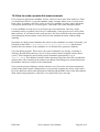
shows the order spectrum of a cogwheel with 34 teeth:
H1
H2
H3
H4
Limit curve
Spectrum
A noise component that is generated from all teeth in the same way is reflected in the
harmonics. A surface defect on all teeth (e.g. not refined, rough or wrong angle, etc.) will
show up with consistently high values in the harmonics.
DISCOM
Noise Analysis User Manual
Page 38 of 63
Candidates of the same type should produce similar noise. The amount similarity is checked
using the (“learned”) limit curve. A candidate that has a measured order spectrum exceeding
the limit curve will sound differently to the previously tested parts. This could be the result of
a change in the manufacturing process (e.g. a tool replacement), but it could also result from a
surface defect (see above) on just some of the teeth of a cogwheel or from surface waviness.
It is worthy to note that measurement values from the order spectrum are not displayed in the
table of measurements. If you suspect that an order is defective you can check this by looking
at the report window (“grey window”). Information concerning any defects and possibly
additional test data is displayed in this window.
12.4 Tracking values of single orders
Some test benches carry out an additional analysis of single spectral components („orders“,
sometimes mesh orders) relative to the rotational speed. This measurement is displayed in a
separate display window.
During the up and down measurement, you
can see how the measurement curve is being
written.
Track_H1 in SK1, Z
dBmm/s
80
There can be limit curves for these curves as
well. Alternatively you can evaluate the
maximum or the mean value of the curve (or
of parts of the curve).
70
60
50
40
Whether such an analysis is performed,
which orders are involved and which kind of
evaluation is being performed, this is defined
in the parameter database.
30
20
0
500
1000
1500
0
500
1000
1500
2000
2500
3000
3500
4000
4500
2000
2500
3000
3500
4000
4500
Track_H1 in SK1, S
dBmm/s
80
70
60
50
40
30
DISCOM
Noise Analysis User Manual
Page 39 of 63
13 Learning Limit Values
13.1 How the Limit Values are
generated
Limit values can be learnt from the statistics of
the production process. Learning is restricted by
settings made in the parameter database and can
even be completely suspended.
Limit values are distinguished by test bench and
candidate. They are stored as files in the folder
C:\RotasData\(Project)\LearnData.
The limit value is calculated using the basic
value and the mean value. Finally, a multiple
value of the standard deviation value is added:
Mean value and standard deviation
Mean value
Distribution of
a value
Standard
deviation.
If you collect a great number of measurements and
depict how often which value has been measured,
you get the distribution of the values. From this you
can calculate the mean value and the standard
deviation. It is defined that 2/3 of the measured
values lie in the area of the standard deviation
around the mean value.
Limit
Limit Value
+ 3 x Standard dev .
Standard deviation
Mean value
+ Mean Value
Basic Value
Measurement Value Statistics
Limit Calculation:
.
Basic Value + Mean + n * Standard dev.
Restricted by database presettings
Learning can be classified into Base Learning and Additional Learning. Base learning
includes only a few candidates (like 5). In the base learning process, the program uses the
maximum value from the database as limit value. At the end of the base learning process,
provisional limits are set.
Additional learning includes a number of candidates (like 100). Each candidate will be
checked using the current limits first. If it is assessed OK, it is added to the statistics. That
way, limit values are finely tuned.
Base Learning
DISCOM
Additional Learning
Noise Analysis User Manual
Limits
set
Page 40 of 63
13.2 Controlling the Learning Process
The learning of spectral limits and of limits for "Energy values“ (Crest, RMS) is controlled by
separate modules in most applications. You can open the dialog for learning control via the
toolbar of the measurement program:
Learn control spectral limits
Learn control Crest/RMS-limits
If you want to learn new limits for a candidate type that is
currently not inserted, select Hand-control in the dialog “Test
status” (see ch.9), select the type for new limit learning and
activate “Subject Ready”.
Open the learning dialog for spectra or for Crest/RMS (see
figure). In this dialog you can see how often the learning
process was started for individual gears.
Select the gear(s) you want to have learnt new and press
“New Learn”.
An asterisk * behind the learning cycle shows the gear is
being learnt new.
If you needed to activate the type of candidate manually,
deactivate „Subject ready” now and set automatic control.
Use alternatively for new learning of all limits: Stop
RotasPro. Go to the project directory
(C:\RotasData\xxxData\), open its subdirectory
LearnData and delete the file corresponding to that type
which shall be leant new. Now restart RotasPro.
DISCOM
Noise Analysis User Manual
Page 41 of 63
14 Testing a new Candidate Type
14.1 How to create a new Candidate Type
RotasPro will only measure candidate types that are defined in the parameter database. If the
test bench issues the message “Insert“, it has to provide a valid type.
Below, as an example, we create a new transfer case type. Please proceed as follows:
1. Start the parameter database (double-click on the D symbol). The main form
of the database appears:
2. Press Create new transfer case type.
DISCOM
Noise Analysis User Manual
Page 42 of 63
3. Enter name of the new type in the entry field in the upper left corner (in the figure
“FCU“) and a new basic number in the field below (that has not been used). Press
Create.
4. Now, the fields in the lower half of the
form become active. Check all the boxes
in the section “This will be copied”.
5. In the dialog “Choice of fields” (opens for
each box that you check) check all boxes
as well.
6. Select a type in the left column “Transfer
case type”, that is mostly similar to the new type. Please make sure that in the right
column “Transfer case type” the new type is selected. Now press >>
7. Close the form.
8. Press Edit Transfer Case Data in the main
form. You will have access to the
following form:
9. Select the new type from the list in the
upper left corner, and press Design data.
DISCOM
Noise Analysis User Manual
Page 43 of 63
10. The form where you can enter design
data opens. The exact appearance of
this form depends on the transfer case
type and its construction. Enter in the
yellow fields the number of teeth for
each cogwheel; the green fields are
being filled with the calculated transmissions.
Now, close all forms. The new type is known
to the system and can be selected by the measurement program.
For further details on the definition of new transfer case types and the maintenance of
parameters, see the database documentation.
14.2 Initial settings / learning of a new type of gearbox
If a completely new type of gearbox comes to your test-bench, proceed as follows:
1. In the database, define the new type as described in the previous section
2. Deactivate the "Hats“ of the spectral limit curves in the measurement program (see
description below).
3. Make tests with at least 10 (different) gearboxes. Preliminary limit curves are learnt by
that.
4. In the database, use the function „Translate hats automatically“ for the new type
(dialog „Edit transfer case data“ – „Channel definition“ – „Translate hats“.)
5. Now, you can re-activate the hats in the measurement program
6. At this moment, preliminary limits have been learnt. These limits can be used at this
stage. Test more gearboxes (100 and more).
7. Let the hats be set automatically again. Use the statistics-tool (see next chapter) to
check and refine the other limit parameters as well.
Step 7 can be seen as a regular task. It should be done frequently in order to have an eye on
quality and evolution of the production.
DISCOM
Noise Analysis User Manual
Page 44 of 63
14.2.1
Switching the Hats on and off in ROTAS
Open the system configuration and find the section Host.
You find the section Limit Curves there (see figure).
Double-click on the module “Spectral Limit Curve SK1”.
The settings dialog for the spectral limit curve opens.
In this dialog, you find the check box Use hats. You can
switch the usage of hats on the limit curve on and off.
If you want to look at the learnt
limit curves, you can select a test
mode in the list and push the
button Show curves.
Remember, that you have to
switch the hats on and off for
each synchronous channel (SK1,
SK2, SK3 …) and for the mix channel separately. You have to open
one dialog for each channel, totalling 4 dialogs at least.
DISCOM
Noise Analysis User Manual
Page 45 of 63
15 How to Use the Statistics Database
The measurement program stores the values from the „long report“ (these are set in the report
list of the parameter database) in the Report database. For each type, the last 1000 measured
values (set individually) are stored.
The statistics tool shows data evaluation:
After the start, you will see the form for selection of
the evaluated database:
First, you need to load the databases you want to
evaluate. You find them in the project directory
(C:\RotasData\xxxData\) in its subdirectory
ProtocolData. For each tested base type, a
separate report database has been created. Per
default, they are named BaseType_prot.
Then, select one or more databases from the list and
press “Display the Data”.
Double-click on a list entry to check the time period covered by the database.
The report database stores only the last, for example, 1000 measurements of each type. If you
want to use a report database over a longer period, it can be useful to copy databases regularly
into another directory to store it.
15.1 Controlling the report database
Open the measurement program and call the report database dialog via
the toolbar button (see figure).
This dialog sets the record-cycle. This is the number of measurements
that the database may hold. (In the figure beside, the last 2000
measurements are held.) The current index shows the position where
the current measurement is being stored. You can see that data has been
stored when the index is incremented at the end of a test. Furthermore,
you can see the name of the current database at the top of the dialog.
Please ensure that the box Report active is checked. For normal
measurements in automatic test mode, the function Record any
analysis separately should be inactive.
In the lower part of the dialog, you can exclude the data of individual
test modes from the storage process. (Double-click on the name of a
test step in the column Mode.) The symbol ‘x’ in the column Report indicates that the values
of this test mode will be stored.
DISCOM
Noise Analysis User Manual
Page 46 of 63
15.2 Creating Evaluations
After you have loaded one or more databases, press the button for display of data. The
evaluation form opens:
Displays the
measurement values
or limits
(For monitoring of
the learning process).
You can enter up to
four values for parallel
display. Enter settings
in each line for
specification of a value.
(Compare them with
the protocol list in the
parameter database.)
Un-checking
temporarily hides the
display of individual
values.
Specifies axis settings.
Press Display or select
Auto scale.
You can carry out two kinds of evaluations: Distribution and Time Series.
The distribution in the bar diagram shows the accumulation of
measured values in certain value intervals (e.g.: the marked bar
shows that ca.40% of the measurements for the blue quantity
are around 85). Use this diagram to set a limit value (or sane
restrictions for the learning process).
A time series shows single measurement values over a certain time
period. Here, tendencies become visible (like slow and quick rise of
values, for example when a tool for tooth production wears off). You
will easily detect accumulations of abnormalities (as peaks in the
curve profile) at certain times. You can have time series printed
using the index (counting of measurements) or using the real time of
the measurement.
DISCOM
Noise Analysis User Manual
Page 47 of 63
15.3 Reproducible Measurements, Reference Measurements and
Calibration
Like with every measurement system, it is desired and required that the measurement values
comply with certain objective criteria. Unfortunately, in acoustics it is not as easy as the
measuring of a weight, for example. If you put a gearbox on a balance, you can measure
objectively that its weight is 31 kg. Each calibrated balance will produce this result as often as
you like.
In the acoustic analysis, the candidate is just one part of a complex system, consisting of test
bench, drives, acoustical sensor and other components. Even two similar test benches are not
identical, and tiny differences have influence on the noise already. Just so, two consecutive
tests are not 100% identical. It’s like picking a guitar string several times: You will produce
similar tones each time but never exactly
Mean value and standard deviation
identical ones. Furthermore, the measured noise
Mean value
is dependant from the system, thus, acoustical
Distribution of
quantities do not have absolute validity (in
a value
Standard
contrast to the weight) but are only valid
deviation.
relative to the test conditions of the test bench.
If you get an (almost) identical result for each
consecutive measurement, you have
If you collect a great number of measurements and
reproducible measurements. It is a quality of the depict how often which value has been measured,
you get the distribution of the values. From this you
whole measurement system and can, as
can calculate the mean value and the standard
described above, only complied within certain
deviation. It is defined that 2/3 of the measured
restrictions as a matter of fact. Thus, you
values lie in the area of the standard deviation
request that the results of different
around the mean value.
measurements must not differ more than a
certain amount (the standard deviation shall be small).
Since the measured values are not absolutely valid, they are compared with other values. (In a
sense you do the same with weighing: You compare a gearbox with something different
where you know how heavy it is.). In practice a so called reference candidate. By testing this
candidate regularly – reference measuring - you make sure that the measured values for the
reference candidate always remain the same (within the standard deviation). You can then
compare the other candidates with the reference candidate.
As mentioned before, the noise of a candidate in the test bench can not be measured
objectively. Nevertheless, the measurement system itself (consisting of noise sensor, amplifier
and measurement PC) can be measured objectively. If you press the noise sensor on a noise
source which produces a noise of 103 dB, you expect the measurement program to show this
value. Verifying this request and – if necessary – adjusting the system is called calibration.
The following sections describe how reproducible measurements are made, how reference
measurements are done and how you calibrate the system. Except for calibration, you need
knowledge about the statistics database tool. Make yourself familiar with this tool before you
start.
DISCOM
Noise Analysis User Manual
Page 48 of 63
15.4 How to make reproducible measurements
First, choose an appropriate candidate. In fact, soft noise varies more than loud noise. Thus,
you should not choose a very good candidate, rather a sample whose noise is nearly at the
limit values. In practise, this is the scope as well: If a candidate is silent, it does not matter
exactly how much silent it is. Near the good – bad border, the results should not differ.
Let the candidate do some tests (ca.10) before the real examination. That way, slight
remainders on the cogwheels can scale off. Additionally, warm gear-boxes are more silent
than cold ones. If you started with a cold gear-box, the noise would become more and more
silent during the measurements, which increases the standard deviation without telling
anything.
Determine in which protocol database the values for this candidate are written. Normally, you
find them in the folder C:\RotasData\(Your Project)\ProtocolData, and the name
includes the base number of the candidate as it is defined in the parameter database.
Close the Rotas-program. Then remove the protocol-database (by moving, renaming or
deleting). Restart Rotas and carry out 10 or more measurements (complete measurement
cycles). Then rename the (newly made) protocol database appropriately (e.g. in
„Repro01.mdb“). This database includes all the data that you need to show the reproducible
measurement. The renaming at the end prevents Rotas from filling more measurements into
the database which are not part of the examination.
Now open the protocol database with the statistics-tool. Choose the relevant measurement
scalars in the main formula. With gearboxes you typically examine the values of the orders
H1 of the different wheels and synchronous channels and the RMS-value in the Mix-channel.
With wheel testing machines, values like Crest and TickEval are relevant.
DISCOM
Noise Analysis User Manual
Page 49 of 63
In the main formula of the statistic-tool you can directly read the mean value and the standard
deviation of the chosen values. Display the time-row and print it out: On this sheet, you see
mean value and standard deviation as well. Furthermore, you can see the dispersion of the
values. These printouts can help you to document the reproducible measurements.
In these fields are displayed the mean value and the
standard deviation of the chosen scalars within the
chosen time interval.
Display the time row. The
lines should not vary much.
15.5 Reference candidates
To ensure the stability of a test bench over a longer period of time, reference candidates are
used in practise. These are selected candidates who are specially marked (e.g. painted red or
green). You should separate its measurements by defining a separate Type-Id (with separate
base-type) in the parameter database (Just make a copy of the settings made for the original
type). If the test bench control tells the measurement program automatically of which type the
current candidate is (e.g. at automatic test benches for gear-boxes), you have to adjust it so
that the new candidate type is issued to the measurement program instead of the original type
of the candidate. If your system has manual selection, the tester himself is responsible for
telling the measurement program that a reference candidate is to be tested.
If you test the reference candidate, its values are collected in a separate protocol database. If
the reference candidate is tested e.g. once a day at the test bench, you can find out with the
statistics-tool (evaluation of the time-row), whether the test bench is stable or whether the
measurement values drift during a period of time. If you make this examination over a longer
period of time you may find seasonable influences as well.
15.6 Calibration
Calibration ensures stability and exactness of the measurement system consisting of sensor,
amplifier and A/D-converter. For calibration you need a calibrator. This is a device which is
able to produce a defined vibration on its surface. You screw a noise sensor on this surface.
Then you can read the value either in the normal measurement program (and make sure that
the system is calibrated right) or you can use a separate calibration program which is
described in a separate handbook.
You check the calibration of a test-bench for gear-boxes with the measurement program as
follows:
DISCOM
Noise Analysis User Manual
Page 50 of 63
1. Disconnect the cable which connects the acceleration sensor with the amplifier and
connect the calibrator to the amplifier instead.
2. Let the test bench and the measurement program run in manual mode. Insert a gear
box on the test bench (the type does not matter) and let the test bench run with a
constant rotational frequency.
3. Insert a type in Rotas manually and switch to one of the test modes. Switch on the
calibrator.
4. Now you should see a distinct peak in the mix spectrum. Use the scaling settings of
the scope to read the exact height of this peak. If you have a standard calibrator with
an effective acceleration of 1g, the maximum value should be at 103 dBg.
Generally, you can assume that the measurement system runs stable for long time periods.
The acceleration sensors and amplifiers that DISCOM uses don’t have a relevant drift.
Nevertheless, it can happen that one of the components is defective (e.g. the amplifier gets out
of order or the tip of the sensor breaks off). But you will notice such defects immediately
because the measurement values will differ dramatically. You should check the calibration
with the measurement program and re-calibrate, if necessary. The other parts of the system
work digital and therefore will not vary.
In practice, reproducible measurements and reference measurements are more important than
calibration. In case, you do not have a calibrator at hand, you can use the measurement system
without restrictions, nevertheless.
16 Backup, Organisation of the Rotas Software
You get the ROTAS PC pre-installed with the RotasPro Software. During the operation of the
Test Bench, there will be changes made in the software (e.g. new types in the database). For
this reason, we advise you to backup the RotasPro-Software in regular intervals.
Maybe you only need to backup a part of the RotasPro-Software (e.g. databases)
16.1 Hard Disk Folders; range of a backup
Rotas Software is located mainly in two
folders: „lDisc“ (=“L-Disc“) and
„RotasData“. LDisc contains the software
itself, RotasData the settings, databases
and learnt values. You may also find
additional folders “Mps32” and
“Dpm42Data” or files like
“XXXXXXRotas.zip” and
“XXXXXXMps32Base.zip”. All these
files and folders must be on top level (C:\).
They must not be moved or renamed.
A full backup should contain all these
folders and files.
DISCOM
Noise Analysis User Manual
Page 51 of 63
Since you do not want to waste backup-space, we advise you to clear up before you make a
backup (see below).
16.2 Organisation of files and folders
All settings and parameters and the learnt values, too are stored in files in the folder
RotasData or its subfolders. (So, if you restore RotasData from a backup copy, all settings
are re-set to the state when the backup was made).
The folder „RotasData“ contains a subfolder for each one of your projects (e.g. for different
production lines, but not for parallel test benches in the same line). In this “project folder” you
find the files and folders listed below.
This list shall give you an overall view and help you to take the right steps in case of
problems. In particular, Rotas install or repair instructions can refer to it
DISCOM
Noise Analysis User Manual
Page 52 of 63
•
•
•
•
•
•
•
•
•
•
RotasApp.sea (sometimes Application.sea) – This file is called “Application-sea”.
All settings that you do within the Rotas program are stored here.
Errcode.set (sometimes with suffixes Errcode-En.set for an English version) – in
this text-file the error codes and error texts are listed. If you want to change a text you can
do it here. If you need to add a new error code, model it on the existing entries.
RotasPro.sea (sometimes RotasProDpm.sea or different suffix) – This filename must
be passed to the Rotas-program as an argument. If you open the properties of the desktoplink (right mouse-button), you will find that it refers to the file RotasPro.sea.
Database – The parameter database files are stored in this folder. They contain the
gear-box construction data, the limit values and further parameters (xxxRatio.mdb,
xxxParams.mdb, xxxEvaluationTables.mdb). Keep in mind, that you cannot open these
database files directly. Use the Desktop-Link „Database“ instead.
•
Backup – In this sub-folder on each change backups of the Rotas database files are
stored (with a preceding consecutive number). In case a change of settings in the
database fails completely, you can restore the state of the last automatic backup as
follows: Move the most recent database files (should be those with the highest number)
into the folder above (Database). Delete the bad database files. Remove the consecutive
number from the moved databases by renaming them.
From time to time, this folder should be cleared up to save space (in particular before
you make a backup)
CacheData – This folder contains temporary database extracts. You can delete the
contents of this folder if you want to make or restore a backup copy.
LearnData – In this folder, the program stores the learnt values and limit curves. You
find for every type a file “Typename.arc”. If you delete one file, the corresponding type
loses its learnt values and limit curves (gets re-taught), except if the program tests this type
at the moment (Thus, close the program before you make changes in this folder).
OrderTracks or Archives – Rotas stores measurement archives (suffix *.rdt) in this
folder. Depending on the settings, this folder should be cleared up from time to time.
PrinterFiles – In this folder, Rotas stores text-files containing the report texts as
they are sent via output line (see chapter Report, normally one file per day). This folder
should be cleared up from time to time as well to save disk space. In particular, if you have
set Rotas to send a „long report” by default.
ProtocolData – In this folder, the protocol databases are stored, ordered by type as
well. These databases can be opened directly or with the statistics-tool.
ProductionData – This folder stores the production statistic. You can open it directly
or with the Rotas program.
DISCOM
Noise Analysis User Manual
Page 53 of 63
16.3 Making a backup copy
Before making a backup copy, you should close all running („open“) components of the Rotas
system. This includes the measurement program RotasPro and the parameter databases, to
ensure that all changes of settings in the measurement program and in the database have been
written to hard disk.
After that you should make a clean-up as described above, if necessary.
Now create a folder with name of your choice (e.g. Rotas220403 for “Rotas backup made
2003 April 3rd”) and copy the folders mentioned above into this folder (pulling with pushed
ctrl-key).
The backup copy is even more valuable if it is stored elsewhere (not on the internal hard disk
of the measurement Pc, but on another Pc via network, on an external hard disk, CD-Rom,
etc).
16.4 Re-storing of a backup copy; Installation of Updates
On Request, you can get a Software-update from DISCOM in order to carry out further
measurements. Before you install them, you should make a backup copy of the current
software as described above. Then you are able to restore the current version if the update
fails.
Please follow an included installation manual absolutely, since it is sometimes necessary to
carry out further preliminary tasks.
Rotas Updates always contain extracts of folders and files mentioned above. Almost always
you will find a folder “lDisc” included often files which have to be written to RotasData.
Before you install a folder lDisc, you should delete existing folders lDisc and Mps32 (have
you been making a backup copy?). To do this, no component of the Rotas software must be
open (like Measurement program or parameter database). Windows warnings can be
answered by “Delete all” or “OK”.
Update-files for the RotasData-folder mostly replace only some existing files. In general,
deleting this folder before an installation is not advisable! (Exception: Re-Installing of a
backup-copy. In this case you should delete the current RotasData folder, because sometimes
a newer software version alters settings in the application sea which do not fit for the prior
version afterwards.
The folder “LDisc” can be included in the update in two ways: Either packed in a Zip-file
XXXXXXRotas.zip or “unpacked” on CD.
-
Unpacking of an XXXXXXRotas.zip: Open the file by double-clicking. Choose
“Extract To” ->C:\. A password is being requested (click Ok). Then the zip-Archive
gets extracted and a folder C:\XXXXXXRotas is being created. At the end, an error
message is displayed which can be ignored (results from the invalid password. A part
of the zip-file is secured by password.). In C:\XXXXXXRotas you will find a folder
“lDisc“, then, which you must move to C:\.
DISCOM
Noise Analysis User Manual
Page 54 of 63
-
„Unpacked“ on CD: Copy all files and folders onto your hard disk (to C:\). They get
the attribute “Read only” from Windows. You need to remove this attribute. You can
do this by right-clicking the folder and choose “Properties” from the menu (Then you
can un-check the property “Read only”). Alternatively, you can use the DOSCommand „attrib -r *.* /s“)
If everything worked fine so far, you should have a folder c:\ldisc on your hard disk now,
which contains the software of the update. To complete the update, you have to execute the
file “Register.bat” in the folder C:\ldisc by double-clicking. All messages must be accepted
with OK (Note: Except on Windows98-systems, you need administrative rights to do this).
In case of problems after a software update, delete the new lDisc etc. and re-install your
backup-copy. Don’t forget to complete this installation by executing Register.bat as well.
DISCOM
Noise Analysis User Manual
Page 55 of 63
17 Appendix
17.1 Complete list of the possible commands from a test bench
The following tables list all valid commands fort the Rotas measurement program. If a
command unknown to Rotas is sent, Rotas will answer with <R>Status: Command? The
following commands are accepted
17.1.1
Exchange of information about the candidate
Command
Insert: Type
Serial: Serial
Serial change:
ChangeSerial: Serial.
Rotas Function
The parameters of a new
candidate are loaded into the
measurement system.
Type is the name of the
candidate (e.g. DP001, DP002).
This name must be defined as
the name of the candidate in the
parameter database. Example:
Insert: DP001
The Rotas system receives the
serial number of the candidate.
This command must be sent
after Insert and before sending
Remove. You can use any string
with a maximum length of 30
characters as serial number.
Answer
The measurement system
answers by sending the line:
<R>Inserted: 1
if the candidate name has been
found in the parameter
database and the parameters
have been successfully loaded
or by sending
<R>Inserted: 0
if the candidate name is
unknown or an error occurred.
This command will not be
answered.
SerialA: Serial
Serial change:
ChangeSerialA: Serial
Insert: Type|Serial
or
Insert: Type|Serial|
ProdType
DISCOM
Function as described above
OK
Combination of the commands This command is answered
Insert and Serial (see above).
like the regular Insert
The type identifier and the serial command (see above).
number are separated by a
vertical line ‘|’.
As an option you can add a piece
of additional information
“ProdType” (e.g. prototype).
Noise Analysis User Manual
Page 56 of 63
17.1.2
Controlling the Test Cycle (Test Step, Measuring)
Command
Mode: Gear
Measure: 1
Measure: 0
MeasureA: 1
MeasureA: 0
Rotas function
The parameters of the test step
Gear are activated by the
measurement system. The
names of the test step must be
defined. The following texts
can be used for a manual
gearbox:
Ramp up:
1-U, 2-U, 3-U, 4-U
Ramp down:
4-D,3-D,2-D,1-D
Switching the evaluation on
and off.
Switching the evaluation on
and off (like above)
MeasureAF: 1
MeasureAF: 0
Switching the evaluation on
and off (like above)
Remove:
The test cycle has been
completed. The Rotas system
prepares the total evaluation
result.
Answer
The successful change of
parameters is answered with the
line
Ready
If the change of parameters did
not succeed, the line
Mode?
is sent.
This command does not have an
answer.
Answer
On for MeasureA: 1 and
Off for MeasureA: 0
Answer
On
for MeasureAF: 1
Of
for MeasureAF: 0
The answer for this command
includes the total evaluation
result:
<R>Result: 1
if the result is o.k.,
<R>Result: 0
Reset
RequestStatus:
if the result is n.o.k.
The system sends the line:
The system aborts the current
<R>Status: Reset
measurement (if necessary)
and takes initial position. No
evaluation is being made.
Enquiry of the measurement’s Rotas sends the line
<R>Status: Online
system state.
if the system reacts to
commands,
<R>Status: Handcontrol
RequestStatusF:
otherwise
Enquiry of the measurement’s Rotas sends the lines
<R>Status: Online
system state.
or
<R>Status: Handct
(See above: RequestStatus).
DISCOM
Noise Analysis User Manual
Page 57 of 63
17.1.3
Receiving Further Information
Command
Timestamp: DateTime
TimeA: DateTime
Rotas function
Setting the time stamp for the
current measurement. Rotas
expects the form:
YYYY MM DD HH MM SS
Answer
No answer.
Rotas sends the line:
OK
(YY will be expanded to 20YY).
Example:
Timestamp: 03 10 04 10 14 02
sets the time stamp Oct 4th 2003,
10:14:02.
SetAddInfo: Key Value
Rotas sends the answer:
Sending information to the
InfoStored
Rotas system which is neither
or
error of value information. The
Rotas system stores the
SetAddInfo: Key1 Value1, information in the archive files.
Each piece of information is
Key2 Value2…
identified by a Key.
ExtError: Code
Rotas sends the answer:
Sending errors to the Rotas
Ready
system which were detected by
or
the test bench. The Rotas system
ExtError: Code1,
stores the information in its
Code2,...,CodeX
database and archive files.
SetRItem: Item
Sending value items to the Rotas Rotas sends the answer:
Ready
system for measurements made
or
by the test bench. The Rotas
SetRItem: Item1,
system stores the information in
Item2,…, ItemX
its database and archive files.
Remark: All commands in the table above may be sent anytime between the Insert and the
Remove command. All commands except the timestamp commands may be sent multiple
times to send different information to the Rotas system.
The commands ExtError and SetRItem accept additional optional information. The form is as
follows (required entries bold):
A Code entry for ExtError has the following form:
ErrorNo|Values|Unit|TestStep|Channel
An Item entry for SetRItem has the following form:
Values|Unit|TestStep|Location|Instrument|Params|Channel|Description
A Values entry for both commands has the following form:
Value#Limit#Average#Position
If an optional entry is not given, defaults will be taken. If a list is sent, the corresponding entry
of the previous item is taken (shortens commands).
DISCOM
Noise Analysis User Manual
Page 58 of 63
17.1.4
Read Out Rotas Defect Information and Evaluation Result
Command
Result:
Result: Gear
Report: Type
Type is
‚Short’ or
‚Long’
Report: Line
or
Report: Line No
Report: ExtCodes
Report: ExtCodFx
Rotas Function
Enquires the (partial) evaluation
result. If the optional parameter
Gear is given, Rotas returns the
evaluation result for that test
step/ gear. Example:
Result: 3-U (for test step 3-U)
Result: 3 (for 3-U and 3-D)
Enquires a report for the last
test. It contains defect
information. The “long” report
contains all measurement values
for all test steps also.
The Rotas system sends only
one line of the long report. As an
option, a line number can be
given to request relevant lines
only. If the command is sent
(without line number) Rotas
send the next line of the report.
The short report ends with two
empty lines. Then, the
measurement values follow. The
long report ends with two empty
lines also.
The Rotas system sends a report
of the external error codes. Up to
50 error codes can be sent.
These error codes can be stored
by the test bench.
Answer
Rotas send the answer
<R>Result: 1
or
<R>Result: 0
Rotas sends the requested
report starting with the line
<D>
The report ends with the line
<\D>
Contents of the requested line
The report starts with the line
<D>
and ends with the line
<\D>
In the report, each error code is
given at the beginning of a
separate line.
The Rotas system sends a report The answer is given in one
of the external error codes. Up to line, starting with <D>. 10
10 error codes can be sent in one three-digit error codes follow.
</D> ends the line. Example:
line. Error codes which are not
<D>00100200300400500600
set are filled with zeros.
7008000000<\D>
8 Errors 1 to 8 are being sent;
the code positions 9 and 10 are
not set.
DISCOM
Noise Analysis User Manual
Page 59 of 63
17.1.5
Read out Rotas Values
Command
GetRItem: Key
Rotas-Function
Answer
Enquires the measurement value Rotas answers:
Value: Value(s)
identified by Key, including
If the requested value has not
limit and position.
been measured, Rotas answers:
No_Val
Remark: The valid keys are a matter of definition.
17.1.6
Displaying Messages
Command
Message: Message
MessageInfo: Message
Rotas Function
Displays a message from the test bench in
Rotas’ message window.
MessageInfo and MessageWarn also set an
adequate background colour.
Answer
No answer
MessageWarn: Message
SeaMessage: Key Arg
Bclr Tclr
17.1.7
Controlling Gear Shift Force Measurement
Command
SGW: gear1 gear2
EGW
Section: name
DISCOM
Displays a predefined message identified by
Key. Arg is an argument for the message.
Bclr and Tclr set individual colours for the
message (Hex: 0xBBGGRR with BB Blue-,
GG Green- and RR Red).
Rotas Function
Indicates a gear shift from gear1
to gear2. The gear names are
“physical” gears, e.g. “R“, “1“,
“2“ etc. “L” and “N” identify the
neutral position.
The gear shift is complete. The
evaluation result of the gear shift
force analysis is returned.
Indicates the start of a
measurement section. Gear shift
force curves are stored with the
appendix name
Noise Analysis User Manual
Answer
Answer:
Ready
Answer:
<R>Result: 1 or 0
Answer:
OK
Example:
Section: SKN
Page 60 of 63
17.1.8
•
•
•
•
•
•
•
•
Remarks:
The system stores all measurement results, error messages, etc., until a new test cycle
is started by sending the Insert command. This means, all kinds of reports (multiple
times either) can be requested after Remove.
The Serial command must be sent between Insert and Remove. If can be sent
repeatedly to change the serial number. The serial number can be any string with less
than 30 Characters.
The valid type identifiers are defined in the parameter database. All other type
identifiers are resigned on the Insert command.
The valid test steps (modes) are also defined in the parameter database. You can skip
test steps if necessary.
The sequence of test steps does not matter to Rotas. You can also repeat test steps. All
results (including errors) of a previous measurement in a certain test step are deleted if
you repeat a test step.
The Rotas program can be configured to control start and stop of the measurement
depending on an analogue signal, e.g. speed. Such configurations don’t need a
Measure:1/ 0 command from the test bench.
The response time for all commands except Insert and Remove are much below 1
second. The Insert command needs more time (up to 10 seconds) if changes have been
made in the parameter database or a completely new candidate type shall be tested.
Otherwise, the Insert command also takes not longer than 2 seconds. The time the
Remove command needs to process depends on the amount of data to store in databaseand archive files, but should be less than 5 seconds.
Additional commands can be defined if special measurements shall be made on single
test benches. See the following chapter for more information:
DISCOM
Noise Analysis User Manual
Page 61 of 63
17.1.9
Special Commands
On request, new commands for special measurements or can be defined. Some commands
don’t differ formally from those listed above. Others are called using the following form:
1) The special command is indicated by the command ExtCmd. The first parameter is the
name of the command. Other parameters define start or stop. (One or more spaces
separate the parameters.)
2) The commands are answered with <R>Result: 1 or 0.
3) It may be necessary to have a test step activated using the mode command. This depends
on the implementation.
Example: Ratio test
At the end of an up ramp (after the acoustical measurement has been completed with the
Measure: 0 command), a ratio test is issued. It tests the gear with has been set with the
previous mode command.
Command
ExtCmd: Ratio Test
Rotas Function
The ratio test is carried out
Answer
Depending on the evaluation
result, the answer is
<R>Result: 1 or 0
Example: Alternate error code list
The Rotas system enters all defect entries into a second error list which can be deleted on
request. This makes it easier for the test bench program to find errors which occurred in a
defined part of the test cycle. The second list contains the same errors than the first one
(which can be enquired with the Report commands). After a special command which resets
the list, it contains only those which occurred after the reset. Both lists are reset on the
Insert command.
Command
ExtCmd: ErrcodeList2 Reset
Rotas Function
Reset of List2
ExtCmd: ErrcodeList2 Report Output of List2
DISCOM
Noise Analysis User Manual
Answer
<R>Result: 1
See
Report: ExtCodFx
Page 62 of 63
DISCOM
Noise Analysis User Manual
Page 63 of 63