Download BornAgain User Manual - Scientific Computing Group

BornAgain
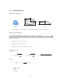
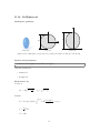
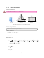
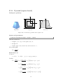
Software for simulating and fitting
X-ray and neutron small-angle scattering
at grazing incidence
User Manual
Version 1.3.0 (July 31, 2015)
Céline Durniak, Marina Ganeva, Gennady Pospelov,
Walter Van Herck, Joachim Wuttke
Scientific Computing Group
Jülich Centre for Neutron Science
at Heinz Maier-Leibnitz Zentrum Garching
Forschungszentrum Jülich GmbH
Homepage:
http://www.bornagainproject.org
Copyright:
Forschungszentrum Jülich GmbH 2013–2015
Licenses:
Software: GNU General Public License version 3 or higher
Documentation: Creative Commons CC-BY-SA
Authors:
Céline Durniak, Marina Ganeva, Gennady Pospelov,
Walter Van Herck, Joachim Wuttke
Scientific Computing Group
at Heinz Maier-Leibnitz Zentrum (MLZ) Garching
Disclaimer:
Software and documentation are work in progress.
We cannot guarantee correctness and accuracy.
If in doubt, contact us for assistance or scientific collaboration.
Contents
Introduction
About BornAgain . . . . . . . . . . . . . . . . . . . . . . . . . . . . . . . . .
About this Manual . . . . . . . . . . . . . . . . . . . . . . . . . . . . . . . . .
Typesetting conventions . . . . . . . . . . . . . . . . . . . . . . . . . . . . . .
5
5
6
6
1 Online documentation
1.1 Download and installation . . . . . . . . . . . . . . . . . . . . . . . . . .
1.2 Further online information . . . . . . . . . . . . . . . . . . . . . . . . . .
1.3 Registration, contact, discussion forum . . . . . . . . . . . . . . . . . . .
8
8
9
9
2 Small-angle scattering and the Born approximation
2.1 Coherent neutron propagation . . . . . . . . . . . . . .
2.2 Neutron scattering in Born approximation . . . . . . .
2.2.1 The Born expansion . . . . . . . . . . . . . . .
2.2.2 Far-field approximation . . . . . . . . . . . . .
2.2.3 Differential cross section . . . . . . . . . . . . .
.
.
.
.
.
.
.
.
.
.
.
.
.
.
.
.
.
.
.
.
.
.
.
.
.
.
.
.
.
.
.
.
.
.
.
.
.
.
.
.
.
.
.
.
.
.
.
.
.
.
10
10
12
12
13
15
3 Grazing-incidence scattering and the distorted wave Born approximation
3.1 Scattering under grazing incidence . . . . . . . . . . . . . . . . . . . . .
3.1.1 Wave propagation in 2 + 1 dimensions . . . . . . . . . . . . . . .
3.1.2 Distorted-wave Born approximation (DWBA) . . . . . . . . . . .
3.2 Absorption . . . . . . . . . . . . . . . . . . . . . . . . . . . . . . . . . .
16
16
16
18
19
4 DWBA for multilayer systems
4.1 Scalar case . . . . . . . . . . . . . . . . . . . . . . . . .
4.1.1 Wave propagation and DWBA matrix element .
4.1.2 Wave propagation across layers . . . . . . . . . .
4.1.3 Damped waves in absorbing media or under total
21
21
21
23
26
. . . . . .
. . . . . .
. . . . . .
reflection
.
.
.
.
.
.
.
.
.
.
.
.
5 Particle Assemblies
27
5.1 Embedded particles . . . . . . . . . . . . . . . . . . . . . . . . . . . . . . 27
A Some proofs
28
A.1 Source–detector reciprocity for scalar waves . . . . . . . . . . . . . . . . 28
3
B Form factor library
B.1 AnisoPyramid (rectangle-based) .
B.2 Box (cuboid) . . . . . . . . . . .
B.3 Cone (circular) . . . . . . . . . .
B.4 Cone6 (hexagonal) . . . . . . . .
B.5 Cuboctahedron . . . . . . . . . .
B.6 Cylinder . . . . . . . . . . . . . .
B.7 EllipsoidalCylinder . . . . . . . .
B.8 FullSphere . . . . . . . . . . . . .
B.9 HemiEllipsoid . . . . . . . . . . .
B.10 FullSpheroid . . . . . . . . . . . .
B.11 Prism3 (triangular) . . . . . . . .
B.12 Prism6 (hexagonal) . . . . . . . .
B.13 Pyramid (square-based) . . . . .
B.14 Ripple1 (sinusoidal) . . . . . . .
B.15 Ripple2 (saw-tooth) . . . . . . .
B.16 Tetrahedron . . . . . . . . . . . .
B.17 TruncatedCube . . . . . . . . . .
B.18 TruncatedSphere . . . . . . . . .
B.19 TruncatedSpheroid . . . . . . . .
.
.
.
.
.
.
.
.
.
.
.
.
.
.
.
.
.
.
.
.
.
.
.
.
.
.
.
.
.
.
.
.
.
.
.
.
.
.
.
.
.
.
.
.
.
.
.
.
.
.
.
.
.
.
.
.
.
.
.
.
.
.
.
.
.
.
.
.
.
.
.
.
.
.
.
.
.
.
.
.
.
.
.
.
.
.
.
.
.
.
.
.
.
.
.
.
.
.
.
.
.
.
.
.
.
.
.
.
.
.
.
.
.
.
.
.
.
.
.
.
.
.
.
.
.
.
.
.
.
.
.
.
.
.
.
.
.
.
.
.
.
.
.
.
.
.
.
.
.
.
.
.
.
.
.
.
.
.
.
.
.
.
.
.
.
.
.
.
.
.
.
.
.
.
.
.
.
.
.
.
.
.
.
.
.
.
.
.
.
.
.
.
.
.
.
.
.
.
.
.
.
.
.
.
.
.
.
.
.
.
.
.
.
.
.
.
.
.
.
.
.
.
.
.
.
.
.
.
.
.
.
.
.
.
.
.
.
.
.
.
.
.
.
.
.
.
.
.
.
.
.
.
.
.
.
.
.
.
.
.
.
.
.
.
.
.
.
.
.
.
.
.
.
.
.
.
.
.
.
.
.
.
.
.
.
.
.
.
.
.
.
.
.
.
.
.
.
.
.
.
.
.
.
.
.
.
.
.
.
.
.
.
.
.
.
.
.
.
.
.
.
.
.
.
.
.
.
.
.
.
.
.
.
.
.
.
.
.
.
.
.
.
.
.
.
.
.
.
.
.
.
.
.
.
.
.
.
.
.
.
.
.
.
.
.
.
.
.
.
.
.
.
.
.
.
.
.
.
.
.
.
.
.
.
.
.
.
.
.
.
.
.
.
.
.
.
.
.
.
.
.
.
.
.
.
.
.
.
.
.
.
.
.
.
.
.
.
.
30
34
36
38
40
42
44
46
48
50
52
54
56
58
60
62
64
66
70
72
Bibliography
74
List of Symbols
75
Index
78
4
Introduction
About BornAgain
BornAgain is a software package to simulate and fit reflectometry, off-specular scattering, and grazing-incidence small-angle scattering (GISAS) of X-rays and neutrons.
It provides a generic framework for modeling multilayer samples with smooth or rough
interfaces and with various types of embedded nanoparticles. Support for neutron
polarization and magnetic scattering is under development. The name, BornAgain,
alludes to the central role of the distorted-wave Born approximation (DWBA) in the
physical description of the scattering process.
BornAgain is being developed by the Scientific Computing Group of the Jülich
Centre for Neutron Science (JCNS) at Heinz Maier-Leibnitz Zentrum (MLZ) Garching,
Germany. It is intended to serve experimentalists in analysing all kinds of reflectometry
data. It is equally aimed at users of MLZ reflectometers [1, 2, 3], at JCNS in-house
researchers, and at the reflectometry and GISAS community at large. It is the main
contribution of JCNS to national [4] and international [5] collaborations of large-scale
facilities for the development of better user software.
BornAgain is released as free and open source software under the GNU General
Public License (GPL, version 3 or higher). This documentation comes under the
Creative Commons license CC-BY-SA.
The converse of this liberal policy is that we cannot guarantee correctness and
accuracy of the code. It is entirely in the responsibility of users to convince themselves
that their data interpretation is physically meaningful and plausible.
BornAgain is still under intense development. New major versions are released
about every two months. When need arises, bugfix versions are released in between.
It is strongly recommended that users regularly update their installations.
The software BornAgain embodies nontrivial scientific ideas. Therefore when
BornAgain is used in preparing scientific papers, it is mandatory to cite the software:
C. Durniak, M. Ganeva, G. Pospelov, W. Van Herck, J. Wuttke (2015),
BornAgain — Software for simulating and fitting X-ray and neutron smallangle scattering at grazing incidence, version […],
http://www.bornagainproject.org
5
The initial design of BornAgain owes much to the widely used program IsGISAXS by
Rémi Lazzari [6, 7]. Therefore when using BornAgain in scientific work, it might be
appropriate to also cite the pioneering papers by Lazzari et al. [6, 8].
Since version 1.0, BornAgain almost completely reproduces the functionality of
IsGISAXS. About 20 exemplary simulations have been tested against IsGISAXS, and
found to agree up to almost the last floating-point digit. BornAgain goes beyond
IsGISAXS in supporting an unrestricted number of layers and particles, diffuse reflection from rough layer interfaces and particles with inner structures. Support for
neutron polarization and magnetic scattering is under development. Adhering to a
strict object-oriented design, BornAgain provides a solid base for future extensions in
response to specific user needs.
About this Manual
This user manual is complementary to the online documentation at http://www.
bornagainproject.org. It does not duplicate information that is more conveniently
read online. Therefore, Sect. 1 just contains a few pointers to the web site. The
remainder of this manual mostly contains background on the scattering theory and
on the sample models implemented in BornAgain, and some documentation of the
corresponding Python functions.
This manual is incomplete. Several important chapters are still missing.
Specifically, we plan to provide documentation on
• X-ray propagation and scattering,
• polarized neutron propagation and magnetic scattering,
• mapping of 𝜕𝜎/𝜕Ω onto flat detectors,
• scattering by rough interfaces,
• scattering by particle assemblies.
We intend to publish these chapters successively, along with new software release. To
avoid confusion, starting with release 1.2 the manual carries the same version number
as the software, even though it is in a less mature state.
We urge users to subscribe to our newsletter (see Sect. 1.3), and to contact us for
any question not answered here or in the online documentation.
We are grateful for all kind of feedback: criticism, praise, bug reports, feature
requests or contributed modules. If questions go beyond normal user support, we will
be glad to discuss a scientific collaboration.
Typesetting conventions
In this manual, we use the following colored boxes to highlight certain information:
6
Such a box contains a warning about potential problems with
the software or the documentation.
This road sign in the margin indicates work in progress.
Such a box contains an implementation note that explains how
the theory exposed in this manual is actually used in BornAgain.
Such a box contains an important fact, for instance an equation
that has a central role in the further development of the theory.
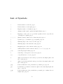
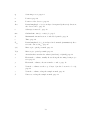
Variations of the equation sign (as ≡, ≔, ≐) are explained in the symbol index,
page 75. See there as well for less common mathematical functions like the cardinal
sine function “sinc”.
7
Chapter 1
Online documentation
This User Manual is complementary to the online documentation at the project web site
http://www.bornagainproject.org. It does not duplicate information that is more
conveniently read online. This brief chapter contains no more than a few pointers to
the web site.
Figure 1.1: A screenshot of the home page http://www.bornagainproject.org.
1.1
Download and installation
BornAgain is a multi-platform software. We actively support the operating systems
Linux, MacOS and Microsoft Windows. The Download section on the BornAgain
8
web site points to the download location for binary and source packages. It also
provides a link to our git server where the unstable development trunk is available for
contributors or for users who want to live on the edge.
The Documentation section contains pages with Installation instructions.
1.2
Further online information
The Documentation section of the project web site contains in particular
• an overview of the software architecture,
• a list of implemented functionality,
• tutorials for “Working with BornAgain”, using either the Graphical User Interface or Python scripts,
• a comprehensive collection of examples that demonstrate how to use BornAgain
for modeling various sample structures and different experimental conditions,
• a link to the API reference for using BornAgain through Python scripts or C++
programs.
1.3
Registration, contact, discussion forum
To stay informed about the ongoing development of BornAgain, register on the project
homepage http://www.bornagainproject.org (“Create new account”). You will
then receive our occasional newsletters, and be authorized to post to the discussion
forum.
To contact the BornAgain development and maintenance team in the Scientific
Computing Group of Heinz Maier-Leibnitz Zentrum (MLZ) Garching, write a mail
to [email protected], or fill the form in the Contact section of the
project web site.
For questions that might be of wider interest, please consider posting to the
discussion forum, accessible through the Forums tab of the project web site.
9
Chapter 2
Small-angle scattering and the Born
approximation
This chapter introduces the basic theory of small-angle scattering (SAS). We specifically consider scalar neutron propagation, adjourning the notationally more involved
vectorial theory of X-rays and polarized neutrons a later edition. Our exposition is
self-contained, except for the initial passage from the microscopic to the macroscopic
Schrödinger equation, which we outline only briefly (Sect. 2.1). The standard description of scattering in first order Born approximation is introduced in a way that is
suitable subsequent modification into the distorted wave Born approximation needed
for grazing-incidence small-angle scattering (Sect.2.2).
2.1
Coherent neutron propagation
The scalar wavefunction 𝜓(𝒓, 𝑡) of a free neutron is governed by the microscopic Schrödinger equation
𝑖ℏ𝜕𝑡 𝜓(𝒓, 𝑡) = {−
ℏ2 2
𝛁 + 𝑉 (𝒓)} 𝜓(𝒓, 𝑡).
2𝑚
(2.1)
By assuming a time-independent potential 𝑉 (𝒓), we have excluded inelastic scattering.
Therefore we only need to consider monochromatic waves with given frequency 𝜔. In
consequence, we have a stationary wavefunction
𝜓(𝒓, 𝑡) = 𝜓(𝒓)e−𝑖𝜔𝑡 .
(2.2)
The minus sign in the exponent of the phase factor is an inevitable consequence of
the standard form of the Schrödinger equation, and is therefore called the quantummechanical sign convention. For electromagnetic radiation usage is less uniform. While
most optics textbooks have adopted the quantum-mechanical convention (2.2), in Xray crystallography the conjugate phase factor e+𝑖𝜔𝑡 is prefered. This crystallographic
sign convention has also been chosen in influential texts on GISAXS (e.g. [8]). Here,
however, we are concerned not only with X-rays, but also with neutrons, and therefore
we need to leave the Schrödinger equation (2.1) intact. Thence:
10
In this manual, and in the program code of BornAgain, the quantum-mechanical
sign convention (2.2) is chosen. This has implications for the sign of the imaginary
part of the refractive index, as explained in Sect. 3.2.
Inserting (2.2) in (2.1), we obtain the stationary Schrödinger equation
{−
ℏ2 2
𝛁 + 𝑉 (𝒓) − ℏ𝜔} 𝜓(𝒓) = 0.
2𝑚
(2.3)
The nuclear (or microscopic) optical potential 𝑉 (𝒓), in a somewhat “naive conception”
[9, p. 7], consists of a sum of delta functions, representing Fermi’s “pseudopotential”.
The superposition of the incident wave with the scattered waves originating from each
illuminated nucleus results in coherent forward scattering, in line with Huygens’ principle.
Coherent superposition also leads to Bragg scattering. However, Bragg scattering
by atomic lattices only occurs at angles far above the small-angle range covered in
GISAS experiments. Accordingly, it can be neglected in the analysis of GISAS data,
or at most, is taken into account as a loss channel.
Therefore, we can neglect the atomic structure of 𝑉 (𝒓), and perform some coarse
graining to arrive at a continuum approximation. This is similar to the passage from
the microscopic to the macroscopic Maxwell equations. The details are intricate [9, 10],
but the result [9, eq. 2.8.32] looks very simple: The macroscopic field equation has still
the form of a stationary Schrödinger equation,
{−
ℏ2 2
𝛁 + 𝑣(𝒓) − ℏ𝜔} 𝜓(𝒓) = 0,
2𝑚
(2.4)
where 𝜓 now stands for the coherent wavefunction obtained by superposition of incident
and forward scattered states, and 𝑣(𝒓) is the macroscopic optical potential. This
potential is weak, and slowly varying compared to atomic length scales. It can be
rewritten in a number of ways, especially in terms of a bound scattering length density
𝜌𝑠 (𝒓) [9, eq. 2.8.37],
𝑣(𝒓) =
2𝜋ℏ2
𝜌 (𝒓),
𝑚 𝑠
(2.5)
or of a refractive index 𝑛(𝒓) defined by
𝑛(𝒓)2 ≔ 1 −
2𝑚
4𝜋
𝜌𝑠 (𝒓) = 1 − 2 2 𝑣(𝒓).
2
𝐾
ℏ 𝐾
(2.6)
In the latter expression, we introduced the vacuum wavenumber 𝐾, which is connected
with the frequency 𝜔 through the dispersion relation
ℏ2 𝐾 2
= ℏ𝜔.
2𝑚
(2.7)
Since we only consider stationary solutions (2.2), 𝜔 will not appear any further in our
derivations. Instead, we use 𝐾 as the given parameter that characterizes the incoming
radiation. In terms of 𝐾 and 𝑛, the macroscopic Schrödinger equation (2.4) can be
rewritten as
11
{𝛁2 + 𝐾 2 𝑛(𝒓)2 } 𝜓(𝒓) = 0.
(2.8)
This equation is the starting point for the analysis of all small-angle scattering experiments, whether under grazing incidence (GISAS) or not (regular SAS).
2.2
Neutron scattering in Born approximation
2.2.1 The Born expansion
To describe an elastic scattering experiment, we need to solve the Schrödinger equation (2.8) under the asymptotic boundary condition
𝜓(𝒓) ≃ 𝜓i (𝒓) + 𝑓(𝜗, 𝜑)
e𝑖𝐾𝑟
for 𝑟 → ∞,
4𝜋𝑟
(2.9)
where 𝜓i (𝒓) is the incident wave as prepared by the experimental apparatus, and
the second term on the right-hand side is the outgoing scattered wave that carries
information in form of the angular distribution 𝑓(𝜗, 𝜑).
For thermal or cold neutrons, as for X-rays, the refractive index 𝑛 is almost always
very close to 1. This suggests a solution of the Schrödinger equation by means of a
perturbation expansion in powers of 𝑛2 − 1. This expansion is named after Max Born
who introduced it in quantum mechanics.1
To carry out this idea, we rewrite the Schrödinger equation once more so that it
takes the form of a Helmholtz equation with a perturbation term on the right side:
(𝛁2 + 𝐾 2 ) 𝜓(𝒓) = 4𝜋𝜒(𝒓)𝜓(𝒓)
(2.10)
with
𝜒(𝒓) ≔
𝐾2
(1 − 𝑛2 (𝒓)) .
4𝜋
(2.11)
This definition just compensates (2.6) so that 𝜒 = 𝜌𝑠 . In the following, we prefer
the notation 𝜒 and the appellation perturbative potential over the scattering length
density 𝜌𝑠 to prepare for the generalization to the electromagnetic case.
Equation (2.10) looks like an inhomogeneous differential equation — provided we
neglect for a moment that the unknown function 𝜓 reappears on the right side. The
homogeneous equation
(𝛁2 + 𝐾 2 ) 𝜓(𝒓) = 0
(2.12)
is solved by plane waves and superpositions thereof. It applies in particular to the
incident wave 𝜓i .
1
It goes back to Lord Rayleigh who devised it for sound, and later also applied it to electromagnetic
waves, which resulted in his famous explanation of the blue sky.
12
For an isolated inhomogeneity,
(𝛁2 + 𝐾 2 ) 𝐺(𝒓, 𝒓′ ) = 𝛿(𝒓 − 𝒓′ )
(2.13)
is solved by the Green function2
′
e𝑖𝐾|𝒓−𝒓 |
,
𝐺(𝒓, 𝒓 ) =
4𝜋|𝒓 − 𝒓′ |
′
(2.14)
which is an outgoing spherical wave centered at 𝒓′ . Convoluting this function with
the given inhomogeneity 4𝜋𝜒𝜓, we obtain what is known as the Lippmann-Schwinger
equation,
𝜓(𝒓) = 𝜓i (𝒓) + ∫d3 𝑟′ 𝐺(𝒓, 𝒓′ )4𝜋𝜒(𝒓′ )𝜓(𝒓′ ).
(2.15)
This integral equation for 𝜓(𝒓) improves upon the original stationary Schrödinger
equation (2.10) in that it ensures the boundary condition (2.9). It can be resolved
into an infinite series by iteratively substituting the full right-hand side of (2.15) into
the integrand. Successive terms in this series contain rising powers of 𝜒. Since 𝜒 is
assumed to be small, the series is likely to converge. In first-order Born approximation,
only the linear order in 𝜒 is retained,
𝜓(𝒓) ≐ 𝜓i (𝒓) + 4𝜋 ∫d3 𝑟′ 𝐺(𝒓, 𝒓′ )𝜒(𝒓′ )𝜓i (𝒓′ ).
(2.16)
This is practically always adequate for material investigations with X-rays or neutrons,
where the aim is to deduce 𝜒(𝒓′ ) from the scattered intensity |𝜓(𝒓)|2 . Since detectors
are always placed at positions 𝒓 that are not illuminated by the incident beam, we are
only interested in the scattered wave field
𝜓s (𝒓) ≔ 4𝜋 ∫d3 𝑟′ 𝐺(𝒓, 𝒓′ )𝜒(𝒓′ )𝜓i (𝒓′ ).
(2.17)
2.2.2 Far-field approximation
We can further simplify (2.17) under the conditions of Fraunhofer diffraction: the
distance from the sample to the detector location 𝒓 must be much larger than the size
of the sample. Since the scattered wave 𝜓s (𝒓) only depends on 𝒓 through the Green
function 𝐺(𝒓, 𝒓′ ), we shall derive a far-field approximation for the latter.
We choose the origin within the sample so that the integral in (2.17) runs over 𝒓′
with 𝑟′ ≪ 𝑟. This allows us to expand
∣𝒓 − 𝒓′ ∣ ≐
√
𝑟2 − 2𝒓 𝒓′ ≐ 𝑟 −
𝒓 𝒓′
𝒌 𝒓′
≡𝑟− f ,
𝑟
𝐾
2
(2.18)
Verification under the condition 𝒓 ≠ 0 is a straightforward exercise in vector analysis. For the
special case 𝒓 = 0, one encloses the origin in a small sphere and integrates by means of the GaussOstrogadsky divergence theorem. This explains the appearance of the factor 4𝜋.
13
where we have introduced the outgoing wavevector
𝒓
𝒌f ≔ 𝐾 .
𝑟
(2.19)
We apply this to (2.14), and obtain in leading order the far-field Green function
𝐺far (𝒓, 𝒓′ ) =
e𝑖𝐾𝑟 ∗ ′
𝜓 (𝒓 )
4𝜋𝑟 f
(2.20)
where
𝜓f (𝒓) ≔ e𝑖𝒌f 𝒓
(2.21)
is a plane wave propagating towards the detector, and 𝜓∗ designates the complex
conjugate of 𝜓. With respect to 𝒓, 𝐺far is an outgoing spherical wave.
The scattered wave (2.17) becomes in the far-field approximation
𝜓s,far (𝒓) =
e𝑖𝐾𝑟
⟨𝜓f |𝜒|𝜓i ⟩ ,
𝑟
(2.22)
where we used Dirac notation for the transition matrix element
⟨𝜓f |𝜒|𝜓i ⟩ ≔ ∫d3 𝑟 𝜓f∗ (𝒓)𝜒(𝒓)𝜓i (𝒓).
(2.23)
In order to reconcile conflicting sign conventions, we will in the following rather use
its complex conjugate ⟨𝜓i |𝜒|𝜓f ⟩ = ⟨𝜓f |𝜒|𝜓i ⟩∗ . Under the standard assumption that the
incident radiation is a plane wave
𝜓i (𝒓) = e𝑖𝒌i 𝒓
(2.24)
with 𝑘i = 𝐾, the matrix element takes the form
⟨𝜓i |𝜒|𝜓f ⟩ = ∫d3 𝑟 𝑒−𝑖𝒌i 𝒓 𝜒(𝒓)𝑒𝑖𝒌f 𝒓 = ∫d3 𝑟 𝑒𝑖𝒒𝒓 𝜒(𝒓) ≕ 𝜒(𝒒),
(2.25)
where we have introduced the scattering vector 3
(2.26)
𝒒 ≔ 𝒌 f − 𝒌i
and the notation 𝜒(𝒒) for the Fourier transform of the perturbative potential, which
is what small-angle neutron scattering basically measures.
3
With this choice of sign, ℏ𝒒 is the momentum gained by the scattered neutron, and lost by the
sample. In much of the literature the opposite convention is prefered, since it emphasizes the sample
physics over the scattering experiment. However, when working with twodimensional detectors it is
highly desirable to express pixel coordinates and scattering vector components with respect to equally
oriented coordinate axes, which can only be achieved by the convention (2.26).
14
2.2.3 Differential cross section
In connection with (2.16) we mentioned that a scattering experiment measures inten2
sities |𝜓(𝒓)| . We shall now restate this in a more rigorous way. In the case of neutron
scattering, one actually measures a probability flux. We define it in arbitrary relative
units as
𝑱(𝒓) ≔ 𝜓∗
𝛁
𝛁
𝜓 − 𝜓 𝜓∗ .
2𝑖
2𝑖
(2.27)
The ratio of the scattered flux hitting an infinitesimal detector area 𝑟2 dΩ to the
incident flux is expressed as a differential cross section
d𝜎
𝑟2 𝐽 (𝒓)
.
≔
dΩ
𝐽i
(2.28)
With (2.24), the incident flux is
(2.29)
𝑱i = 𝒌i .
With (2.22), the scattered flux at the detector is
𝑱(𝒓) = 𝒓̂
𝐾
|⟨𝜓 |𝜒|𝜓f ⟩|2 .
𝑟2 i
(2.30)
From (2.28) we obtain the generic differential cross section of elastic scattering in first
order Born approximation,
d𝜎
2
= |⟨𝜓i |𝜒|𝜓f ⟩| .
dΩ
(2.31)
As we shall see below, it holds not only for plane waves governed by the vacuum
Helmholtz equation (2.12), but also for distorted waves.
In the plane-wave case (2.25) considered here, the differential cross section is just
the squared modulus of the Fourier transform of the perturbative potential,
d𝜎
= |𝜒(𝒒)|2 .
dΩ
(2.32)
15
Chapter 3
Grazing-incidence scattering and the
distorted wave Born approximation
In this chapter, introduce grazing-incidence small-angle scattering and its standard
theoretical treatment by means of the distorted wave Born approximation (Sect. 3.1).
We also discuss the treatment of absorption (Sect. 3.2).
3.1
Scattering under grazing incidence
3.1.1 Wave propagation in 𝟐 + 𝟏 dimensions
Reflectometry and grazing-incidence scattering are designed for the investigation of
surfaces, interfaces, and thin layers, or most generically: samples with a 2 + 1 dimensional structure that are on average translationally invariant in 𝑥 and 𝑦 direction, but
structured in 𝑧 direction. By convention, we designate the sample plane (𝑥𝑦) as horizontal, and the sample normal (𝑧) as vertical, even if this does not correspond to the
actual experimental geometry.1 The 𝑧 axis points upwards, hence out of the sample
towards the vacuum (or air) halfspace where the incident radiation comes from, as
illustrated in Fig. 3.1.
Vertical modulations of the refractive index 𝑛(𝒓) cause refraction and reflection
of an incident plane wave. For small glancing angles, these distortions can be arbitrary
large, up to the limiting case of total reflection, even though 1 − 𝑛 is only of the order
10−5 or smaller. Such zeroth-order effects cannot be accounted for by perturbative
scattering theory. Instead, we need to deal with refraction and reflection at the level
of the wave propagation equation. We move the vertical variations of the squared
refractive index to the left-hand side of the Schrödinger equation (2.8),
{𝛁2 + 𝐾 2 𝑛2 (𝑧)} 𝜓(𝒓) = 4𝜋𝜒(𝒓)𝜓(𝒓),
(3.1)
where the overline indicates an horizontal average. Deviating from (2.11), the perturbation has been redefined as
𝜒(𝒓) ≔
𝐾2 2
(𝑛 (𝑧) − 𝑛2 (𝒓)) ,
4𝜋
(3.2)
1
In many reflectometers, the scattering plane and the sample normal are horizontal in laboratory
space.
16
Figure 3.1: Geometric conventions in GISAS scattering comprise a Cartesian coordinate system
and a set of angles. The coordinate system has a 𝑧 axis normal to the sample plane, and pointing
into the halfspace where the beam comes from. The 𝑥 axis usually points along the incident
beam, projected onto the sample plane. Incident and final plane waves are characterized by
wavevectors 𝒌i , 𝒌f ; the angle 𝛼i is the incident glancing angle; 𝜙i is usually zero, unless used
to describe a sample rotation; 𝛼f is the exit angle with respect to the sample’s surface; and 𝜙f
is the scattering angle with respect to the scattering plane. The numbered layers illustrate a
multilayer system as dicussed in Sect. 4.
which only accounts for horizontal fluctuations of the refractive index. Wave propagation, unperturbed by 𝜒, but including refraction and reflection effects, obeys the
homogeneous equation
{𝛁2 + 𝐾 2 𝑛2 (𝑧)} 𝜓(𝒓) = 0.
(3.3)
It is solved for the horizontal coordinate 𝒓∥ by the factorization ansatz
𝜓(𝒓) = e𝑖𝒌∥ 𝒓∥ 𝜙(𝑧).
(3.4)
The horizontal wavevector 𝒌∥ remains constant as initialized by the incoming beam.
The vertical wavefunction must fulfill
{𝜕𝑧2 + 𝐾 2 𝑛2 (𝑧) − 𝑘∥2 } 𝜙(𝑧) = 0.
(3.5)
When an incident plane wave, travelling downwards with 𝜙(𝑧) = e−𝑖𝑘⟂ 𝑧 , impinges
on a sample with 𝑛2 (𝑧) ≠ 1, then the wave is partly reflected (−𝑘⟂ reversed into
17
+𝑘⟂ ) and partly refracted (𝑘⟂ changing while 𝒌∥ stays constant, resulting in a change
of glancing angle). Similarly, reflection and refraction occur whenever 𝑛2 (𝑧) varies
within the sample. As a result, at any 𝑧 within the zone where 𝑛2 (𝑧) varies, the
vertical wavefunction 𝜙(𝑧) is composed of a downward travelling component 𝜙− (𝑧) and
an upward travelling component 𝜙+ (𝑧).
For a graded refractive index 𝑛2 that is a smooth function of 𝑧, the differential
equation (3.5) is best solved using the WKB method.2 If otherwise 𝑛2 (𝑧) is discontinuous at some interface 𝑧 = 𝑧𝑗 , then the limiting values of 𝜙− (𝑧) and 𝜙+ (𝑧) on
approaching 𝑧𝑗 from above or below are connected to each other through Fresnel’s
transmission and reflection coefficients. This applies in particular to multilayer systems, discussed in chapter 4.
3.1.2 Distorted-wave Born approximation (DWBA)
The standard form of the Born approximation, as presented in Sect. 2.2, combines
an approximation scheme (computing (2.15) by iteration) with an assumption (the
incident field is a plane wave) and an analytic result (in far-field approximation, the
Green function of the Helmholtz equation is a plane wave with respect to the locus of
scattering). These three elements must not necessarily go together. We can apply the
very same approximation scheme, even if the incident field is not a plane wave, but
a distorted wave, namely a superposition of downwards and upwards travelling plane
waves, as derived in the previous section. This is the core idea of the distorted-wave
Born approximation (DWBA).3
To carry out this idea, we need to determine the Green function 𝐺. In Sect. 2.2.1
we did so quite specifically for a homogeneous material. Computing 𝐺 in closed form for
a more generic wave equation like (3.3) is far more difficult, if not outright impossible.
Fortunately, this computation is not necessary, and would be but wasted effort: We do
not need the full solution 𝐺(𝒓, 𝒓′ ), but only its asymptotic far-field value 𝐺(𝒓D , 𝒓′ ) at
a detector position 𝒓D . Thanks to a source-detector reciprocity theorem (A.10) proven
in Appendix A.1, we can compute this value as
(3.6)
𝐺(𝒓D , 𝒓) = 𝐵(𝒓, 𝒓D ),
where 𝐵 is the adjoint Green function that describes backward propagation from 𝒓D
into the sample.
Outside the sample, 𝐵 obeys the Helmholtz equation with isolated inhomogeneity
(2.13), and therefore has the far-field expansion (2.20),
𝐵far (𝒓, 𝒓D ) =
e𝑖𝐾𝑟D −𝑖𝒌f 𝒓
e
.
4𝜋𝑟D
(3.7)
When this backward propagating plane waves impinges on the sample, it undergoes
reflection and refraction in exactly the same way as the incident plane wave e𝑖𝒌i 𝒓 .
2
Also called semiclassical approximation or phase integral method, named after Wentzel (1926),
Kramers (1926), Brillouin (1926). See any textbook on quantum mechanics.
3
The distorted-wave Born approximation was originally devised by Massey and Mott (ca 1933) for
collisions of charged particles.
18
Therefore, (3.7) admits a generalization that also holds inside the sample:
𝐵far (𝒓, 𝒓D ) =
e𝑖𝐾𝑟D ∗
𝜓 (𝒓).
4𝜋𝑟D f
(3.8)
Applying now the reciprocity theorem (3.6), we obtain
𝐺far (𝒓, 𝒓′ ) =
e𝑖𝐾𝑟 ∗ ′
𝜓 (𝒓 )
4𝜋𝑟 f
(3.9)
which agrees literally with (2.20), though 𝜓f is not any longer a plane wave. Accordingly, the scattered far-field is still given by (2.22), and the differential cross section
by (2.31). We only need to redetermine the matrix element ⟨𝜓i |𝜒|𝜓f ⟩, which no longer
has the plane-wave form (2.25).
Since both the incident and the scattered distorted wavefunction are composed of
downward and upward propagating waves,
−
+
(𝒓) + 𝜓𝑤
(𝒓)
𝜓𝑤 (𝒓) = 𝜓𝑤
with
𝑤 = i, f,
(3.10)
the matrix element can be expanded into four terms,
⟨𝜓i |𝜒|𝜓f ⟩ = ⟨𝜓i− |𝜒|𝜓f− ⟩ + ⟨𝜓i− |𝜒|𝜓f+ ⟩ + ⟨𝜓i+ |𝜒|𝜓f− ⟩ + ⟨𝜓i+ |𝜒|𝜓f+ ⟩ ,
(3.11)
or in an obvious shorthand notation
⟨𝜓i |𝜒|𝜓f ⟩ = ∑ ∑ ⟨𝜓i± |𝜒|𝜓f± ⟩ .
±i
(3.12)
±f
This equation contains the essence of the distorted-wave Born approximation for smallangle scattering under grazing incidence, and is the base for all scattering models
implemented in BornAgain. Since ⟨𝜓i |𝜒|𝜓f ⟩ appears as a squared modulus in the
differential cross section (2.31), the four terms of (3.12) can interfere with each other,
which adds to the complexity of GISAS patterns.
3.2
Absorption
The complex refractive index of a given material shall be written as
(3.13)
𝑛 ≐ 1 − 𝛿 + 𝑖𝛽,
introducing two small real parameters 𝛿, 𝛽. However, in our derivations, which are all
rooted in (2.8), 𝑛 only appears as 𝑛2 . Therefore, we actually define
𝑛2 ≔ 1 − 2𝛿 + 2𝑖𝛽,
(3.14)
and read (3.13) as an excellent approximation.
While the real part of 𝑛 is responsible for refraction, reflection, and scattering, the
imaginary part describes absorption and leads to a damping of propagating waves. The
19
plus sign in front of the imaginary part is a consequence of the quantum-mechanical
sign convention; in the X-ray crystallography convention it would be a minus sign.
The factorization ansatz (3.4) leaves us some freedom how to deal with an imaginary part of 𝑛. We choose that horizontal wavevectors 𝒌∥ shall always be real. The
damping then appears in the vertical wavefunction 𝜙(𝑧) that is governed by the complex wave equation (3.5).
20
Chapter 4
DWBA for multilayer systems
In Sect. 3.1, we have discussed wave propagation and scattering in 2+1 dimensional
systems that are translationally invariant in the horizontal 𝑥𝑦 plane, and have a vertical
refractive index profile 𝑛2 (𝑧). Here we specialize to layered systems where 𝑛2 (𝑧) is a
step function that is constant within one layer. First, only scalar interactions are
considered. Later, the theory is extended to account for polarization effects.
By convention, layers are numbered from top to bottom (see Fig. 4.1). The
top vacuum (or air) layer (which extends to 𝑧 → +∞) has number 0, the substrate
(extending to 𝑧 → −∞) is layer 𝑁 .
All layer interfaces are assumed to be perfectly smooth. Support for rough interfaces is already implemented in BornAgain, but documentation is adjourned to a later
edition of this manual.
4.1
Scalar case
4.1.1 Wave propagation and DWBA matrix element
To compute scattering cross sections in DWBA, we first need to determine the distorted
wavefunctions 𝜓𝑤 (𝒓) for 𝒓 inside the sample. The following derivation holds for the
incoming wave (𝑤 = i) as well as for the back-traced detected wave (𝑤 = f).
We consider wave propagation in one layer 𝑙 with constant average refractive
index 𝑛2 (𝑧) = 𝑛2𝑙 . A vacuum plane wave, impinging on a layered structure, is at each
interface partly reflected, partly refracted, so that the wavefunction inside a material
layer has an upward and a downward propagating component, as per (3.10). Each
component is a plane wave, with a wavevector
𝒌±
𝑤𝑙 = 𝒌∥𝑤 ± 𝑘⟂𝑤𝑙 𝒛.̂
(4.1)
As explained in connection with (3.4), the in-plane wavevector 𝒌∥𝑤 remains constant
across layer interfaces. The vertical wavenumber is obtained from (3.5),
2 .
𝑘⟂𝑤𝑙 = √𝐾 2 𝑛2𝑙 − 𝑘∥𝑤
(4.2)
21
z
layer 0
air/vacuum
z0 = z1
layer 1
z2
· · ·
···
zN−1
layer N−1
zN
layer N
substrate
Figure 4.1: The parameter 𝑧𝑙 is the 𝑧 coordinate of the top interface of layer 𝑙, except for 𝑧0
which is the coordinate of the bottom interface of the air/vacuum layer 0.
We factorize the corresponding wavefunctions as
±
±
𝜓𝑤𝑙
(𝒓) = e𝑖𝒌∥𝑤 𝒓∥ 𝜙𝑤𝑙
(𝑧),
(4.3)
with vertical propagation described by a one-dimensional wavefunction
±
±𝑖𝑘⟂𝑤𝑙 (𝑧−𝑧𝑙 )
𝜙𝑤𝑙
(𝑧) = 𝐴±
.
𝑤𝑙 e
(4.4)
For later convenience, the phase factor in (4.4) includes an offset 𝑧𝑙 as defined in
Fig. 4.1. The amplitudes 𝐴 are often written with distinct letters T and R to designate
the transmitted or reflected beam,
𝑅𝑤𝑙 ≔ 𝐴+
𝑤𝑙 .
𝑇𝑤𝑙 ≔ 𝐴−
𝑤𝑙 ,
(4.5)
They need to be computed recursively, as described in the following subsection 4.1.2.
In the absence of absorption, wavevectors are real so that we can describe the
beam in terms of a glancing angle
(4.6)
𝛼𝑤𝑙 ≔ arctan(𝑘⟂𝑤𝑙 /𝑘∥𝑤 ).
Equivalently,
(4.7)
𝑘∥𝑤 = 𝐾𝑛𝑙 cos 𝛼𝑤𝑙 .
Since 𝑘∥𝑤 is constant across layers, we have
𝑛𝑙 cos 𝛼𝑤𝑙 = the same for all 𝑙,
(4.8)
which is Snell’s refraction law.
±
Since the 𝜓𝑤𝑙
are plane waves within layer 𝑙, we can at once write down the
DWBA transition matrix element (3.12)
±
±
±
⟨𝜓i |𝜒|𝜓f ⟩ = ∑ ∑ ∑ 𝐴±∗
i𝑙 𝐴f𝑙 𝜒𝑙 (𝒌f𝑙 − 𝒌i𝑙 ),
𝑙
±i
±f
22
(4.9)
where
𝑧𝑙−1
𝜒𝑙 (𝒒) ≔ ∫
d𝑧 ∫d2 𝑟∥ e𝑖𝒒 𝒓 𝜒(𝒓)
(4.10)
𝑧𝑙
is the Fourier transform of the perturbative potential (3.2), restricted to one layer.
To alleviate later calculations, we now number the four DWBA terms from 1 to
4, and define the corresponding wavenumbers and amplitude factors and as
−
𝒒 1 ≔ 𝒌−
f − 𝒌i ,
−
𝐶 1 ≔ 𝐴−∗
i 𝐴f ,
+
𝒒 2 ≔ 𝒌−
f − 𝒌i ,
+
𝐶 2 ≔ 𝐴−∗
i 𝐴f ,
−
𝒒 3 ≔ 𝒌+
f − 𝒌i ,
−
𝐶 3 ≔ 𝐴+∗
i 𝐴f ,
+
𝒒 4 ≔ 𝒌+
f − 𝒌i ,
+
𝐶 4 ≔ 𝐴+∗
i 𝐴f .
(4.11)
Accordingly, we can write (4.9) as
⟨𝜓i |𝜒|𝜓f ⟩ = ∑ ∑ 𝐶𝑙𝑢 𝜒𝑙 (𝒒𝑙𝑢 ).
𝑙
(4.12)
𝑢
From (4.1) we see that all four wavevectors 𝒒𝑢 have the same horizontal component,
𝑢
𝒒 𝑢 = 𝒒∥ + 𝑞⟂
𝒛̂
(4.13)
whence the vertical components
1
𝑞⟂
= +𝑘f⟂ − 𝑘i⟂ ,
2
𝑞⟂
= +𝑘f⟂ + 𝑘i⟂ ,
(4.14)
3
𝑞⟂
= −𝑘f⟂ − 𝑘i⟂ ,
4
𝑞⟂
= −𝑘f⟂ + 𝑘i⟂ .
4.1.2 Wave propagation across layers
The plane-wave amplitudes 𝐴±
𝑤𝑙 need to be computed recursively from layer to layer.
Since these computations are identical for incident and final waves, we omit the subscript 𝑤 in the remainder of this section. At layer interfaces, the optical potential
changes discontinuously. From elementary quantum mechanics we know that piecewise
solutions of the Schrödinger equations must be connected such that the wavefunction
𝜙(𝒓) and its first derivative 𝛁𝜙(𝒓) evolve continuously.
To deal with the coordinate offsets introduced in (4.4), we introduce the function
(4.15)
𝑑𝑙 ≔ 𝑧𝑙 − 𝑧𝑙+1 ,
which is the thickness of layer 𝑙, except for 𝑙 = 0, where the special definition of
𝑧0 (Fig. 4.1) implies 𝑑0 = 0. We consider the interface between layers 𝑙 and 𝑙 − 1,
23
z
···
Ml−1
Φl−1
layer l−1
Ml
Φl
layer l
Ml+1
zl−1
dl−1
zl
dl
zl+1
···
Figure 4.2: The transfer matrix 𝑀𝑙 connects the wavefunctions Φ𝑙 , Φ𝑙−1 in adjacent layers.
with 𝑙 = 1, … , 𝑁 , as shown in Fig. 4.2. This interface has the vertical coordinate
𝑧𝑙 = 𝑧𝑙−1 − 𝑑𝑙−1 . Accordingly, the continuity conditions at the interface are
𝜙𝑙 (𝑧𝑙 ) =
𝜙𝑙−1 (𝑧𝑙−1 − 𝑑𝑙−1 ),
𝜕𝑧 𝜙𝑙 (𝑧𝑙 ) = 𝜕𝑧 𝜙𝑙−1 (𝑧𝑙−1 − 𝑑𝑙−1 ).
(4.16)
We abbreviate
𝑓𝑙 ≔ 𝑘⟂𝑙 /𝐾 = √𝑛2𝑙 − (𝑘∥ /𝐾)2
(4.17)
𝛿𝑙 ≔ e𝑖𝐾𝑓𝑙 𝑑𝑙 .
(4.18)
and
For the plane waves (4.4), the continuity conditions (4.16) take the form
+𝐴−
+𝐴+
𝑙
𝑙
= +𝐴−
𝑙−1 𝛿𝑙−1
∗
+𝐴+
𝑙−1 𝛿𝑙−1 ,
+
+
−
∗
−𝐴−
𝑙 𝑓𝑙 +𝐴𝑙 𝑓𝑙 = −𝐴𝑙−1 𝛿𝑙−1 𝑓𝑙−1 +𝐴𝑙−1 𝛿𝑙−1 𝑓𝑙−1 .
(4.19)
After some lines of linear algebra, we can rewrite this equation system as
(
𝐴−
𝑙−1
𝐴+
𝑙−1
) = 𝑀𝑙 (
𝐴−
𝑙
𝐴+
𝑙
(4.20)
)
with the transfer matrix
𝑀𝑙 ≔ (
∗
𝛿𝑙−1
0
0
𝛿𝑙−1
)
(𝑓
+ 𝑓𝑙 ) (𝑓𝑙−1 − 𝑓𝑙 )
1
( 𝑙−1
).
2𝑓𝑙−1
(𝑓𝑙−1 − 𝑓𝑙 ) (𝑓𝑙−1 + 𝑓𝑙 )
(4.21)
In a scattering setup, plane-wave amplitudes are subject to two boundary conditions. Let us assume that the source or the sink is located at 𝑧 > 0. Then in the
top layer, 𝐴−
0 = 1 is given by the incident or back-traced final plane wave. In the
substrate, 𝐴+
𝑁 = 0 because there is no radiation coming from 𝑧 → −∞. This leaves
24
us with two unkown amplitudes, the overall coefficients of transmission 𝐴−
𝑁 and re+
flection 𝐴0 . These two unknowns are connected by a system of two linear equations,
(
1
𝐴+
0
) = 𝑀1 ⋯ 𝑀 𝑁 (
𝐴−
𝑁
0
(4.22)
).
While it is possible in principle to solve this as a matrix equation, the actual implementation in BornAgain starts with a unit vector in the substrate, and then carries out
the propagation step (4.20) interface by interface, yielding unnormalized amplitudes
(
̃
𝐴−
1
𝑙
) ≔ 𝑀𝑙+1 ⋯ 𝑀𝑁 ( ) .
+
̃
𝐴𝑙
0
(4.23)
When the top layer is reached, the obtained values are renormalized so that the boundary condition 𝐴−
0 = 1 be satisfied,
𝐴±
𝑙 =
̃
𝐴±
𝑙
.
𝐴−̃
(4.24)
0
For GISAS detection in transmission geometry (sink location 𝑧 < 0) all the development following (4.21) holds with exchanged order of layers: (0, … , 𝑁 ) ↦ (𝑁 , … , 0).
GISAS in transmission geometry is not yet implemented in BornAgain, but high on
our agenda.
At this point, it may be an interesting exercise to make a connection with a well
known textbook result. Consider a system with a single interface between two semiinfinite media. A straightforward computation will show that the transmission and
reflection probabilities determined as above agree with Fresnel’s result for 𝑠-polarized
light,1
2
2
|𝐴−
𝑁| = ∣
2𝑓0
∣ ,
𝑓0 + 𝑓1
2
∣𝐴+
0∣ = ∣
2
𝑓0 − 𝑓1
∣ .
𝑓0 + 𝑓1
(4.25)
The above algorithm fails if 𝑓𝑙 → 0 because 𝑀𝑙+1 becomes singular. A layer with
𝑓𝑙 = 0 only sustains horizontal wave propagation; radiation from below or above is
totally reflected at its boundaries. In BornAgain, such total reflection is imposed if |𝑓𝑙 |
falls below a very small value (currently 10−20 ). However, except for the top vacuum
layer this ought to be inconsequential because the index of refraction should always
have an absorptive component that prevents 𝑓𝑙 from becoming zero.
1
See any optics textbook, e.g. Born & Wolf [11, ch. 1.5.2] or Hecht [12, ch. 4.6.2].
25
4.1.3 Damped waves in absorbing media or under total reflection
In Sect. 3.2, we have chosen the horizontal wavevector 𝒌∥ to be always real and constant.
In contrast, the vertical wavenumber 𝑘⟂𝑙 , given by (4.2), can become imaginary or
complex. If 𝑛2𝑙 is real and smaller than 𝑛20 cos2 𝛼0 , then Snell’s law of refraction (4.8)
cannot be fulfilled, and the radicand in (4.2) becomes negative so that 𝑘⟂𝑙 becomes
pure imaginary. If the layer is absorbing, described by a positive imaginary part of
𝑛2𝑙 , then the radicand in (4.2) becomes complex, and the wavenumber 𝑘⟂𝑙 as well. For
complex 𝑘⟂𝑙 , the theory developed above remains applicable, except that the geometric
interpretation of the wavevectors 𝒌± in Eqs. (4.6–4.8) is untenable.
Writing
′
″
𝑘⟂ = 𝑘⟂
+ 𝑖𝑘⟂
(4.26)
for a decomposition into a real and an imaginary part, we find an exponential decay
of the plane wave amplitudes
″
∣𝜙𝑙± (𝑧)∣ = e∓𝑘⟂𝑙 𝑧
(4.27)
along their propagation direction ±𝑧. With an analogous decomposition of the threedimensional wavevector (4.1), we obtain for the flux, defined as in (2.27),
𝑱𝑙 (𝒓) = 𝒌′ e−2𝑘⟂𝑙 𝑧 .
(4.28)
In the special case of a pure imaginary 𝑘⟂𝑙 , the flux direction is 𝒌′ = 𝒌∥ . Then 𝜓𝑙 (𝒓)
is an evanescent wave, travelling horizontally. Since a stationary evanescent wave
implies that there is no vertical energy transport, all incoming radiation undergoes
total reflection.
In the generic case of a complex 𝑘⟂𝑙 , the flux has a vertical component. Accordingly, the total reflection is not perfect. Some intensity is dissipated in layer 𝑙. And
if layer 𝑙 < 𝑁 is not too thick, then some radiation intensity also tunnels into the
adjacent layer 𝑙 + 1.
26
Chapter 5
Particle Assemblies
5.1
Embedded particles
In many important GISAS applications, fluctuations of the refractive index are due
to islands, inclusions or holes of a mesoscopic size (nanometer to micrometer). In the
following, all such inhomogeneities will be described as particles that are embedded in
a material layer.
Documentation on inter-particle correlations is under preparation. BornAgain currently offers the same choice of models as IsGISAXS. Therefore, for the moment we
refer to the IsGISAXS manual [7].
Implemented particle form factors are described in Appendix B.
27
Appendix A
Some proofs
This appendix contains proofs that were taken out of the main text in order not to
disrupt the physics narration.
A.1
Source–detector reciprocity for scalar waves
We derive a source-detector reciprocity theorem for the scalar Schrödinger equation.
It is needed in the derivation of the distorted-wave Born approximation (Sect. 3.1.2),
where it allows us to short-cut the computation of the Green function, yielding at once
the far-field at the detector position.
We start from a generic stationary Schrödinger equation with an isolated inhomogeneity,
{𝛁2 + 𝑣(𝒓)} 𝐺(𝒓, 𝒓S ) = 𝛿(𝒓 − 𝒓S ).
(A.1)
We assume that the source location 𝒓S (which in our application is a scattering center)
lies within a finite sample volume. Outside the sample, the potential 𝑣(𝒓) has the
constant value 𝐾 2 so that (A.1) reduces to the Helmholtz equation
{𝛁2 + 𝐾 2 } 𝐺(𝒓, 𝒓S ) = 0.
(A.2)
We introduce the adjoint Green function 𝐵 that originates from a source term at the
detector location and obeys
{𝛁2 + 𝑣(𝒓)} 𝐵(𝒓, 𝒓D ) = 𝛿(𝒓 − 𝒓D ).
(A.3)
We also introduce the auxiliary vector field
𝑿(𝒓, 𝒓S , 𝒓D ) ≔ 𝐵(𝒓, 𝒓D )𝛁𝐺(𝒓, 𝒓S ) − 𝐺(𝒓, 𝒓S )𝛁𝐵(𝒓, 𝒓D ).
(A.4)
We inscribe the sample, the detector, and the origin of the coordinate system into a
sphere 𝒮 with radius 𝑅, and compute the volume integral
𝐼(𝒓S , 𝒓D ) = ∫d3 𝑟 𝛁𝑿(𝒓, 𝒓S , 𝒓D )
𝒮
= ∫d3 𝑟 (𝐵𝛁2 𝐺 − 𝐺𝛁2 𝐵)
𝒮
= 𝐵(𝒓S , 𝒓D ) − 𝐺(𝒓D , 𝒓S ).
28
(A.5)
Alternatively, we can compute 𝐼 as a surface integral
𝐼(𝒓S , 𝒓D ) = ∫ d𝝈 𝑿(𝒓, 𝒓S , 𝒓D ) = ∫ d𝜎 (𝐵𝜕𝑅 𝐺 − 𝐺𝜕𝑅 𝐵) .
𝜕𝒮
(A.6)
𝜕𝒮
On the surface 𝜕𝒮, 𝐵 and 𝐺 are outgoing wave fields that obey the Helmholtz equation.
Solutions of this equation in spherical coordinates have a well-known series expansion.
We send 𝑅 → ∞ so that we need only to retain the lowest order, the form of which
has been anticipated in the boundary condition (2.9),
𝐺(𝒓(𝑅, 𝜗, 𝜑), 𝒓S ) ≐
e𝑖𝐾𝑅
𝑔(𝜗, 𝜑),
4𝜋𝑅
(A.7)
e𝑖𝐾𝑅
𝑏(𝜗, 𝜑).
4𝜋𝑅
(A.8)
and similarly
𝐵(𝒓(𝑅, 𝜗, 𝜑), 𝒓D ) ≐
The functions 𝑔 and 𝑏 can be further expanded into spherical harmonics, but this is of
no interest here. The decisive point is the factorization of 𝐺 and 𝐵 and their common
𝑅 dependence. It follows at once that
𝐼(𝒓S , 𝒓D ) = ∫ d𝜎 (𝑅-dependent)(𝑏𝑔 − 𝑔𝑏) = 0.
(A.9)
𝜕𝒮
From (A.5) we obtain the reciprocity theorem
(A.10)
𝐺(𝒓D , 𝒓S ) = 𝐵(𝒓S , 𝒓D ).
It allows us to obtain the far-field value of the forward-propagating Green function 𝐺
at the detector position 𝒓D from the adjoint Green function 𝐵 that traces the radiation
back from 𝒓D to the source location 𝒓S . The theorem is practically important because
𝐵 is much easier to compute than the unexpanded 𝐺.
29
Appendix B
Form factor library
BornAgain comes with a comprehensive collection of hard-coded shape transforms for
standard particle geometries like spheres, cylinders, prisms, pyramids or ripples. This
collection is documented in the following. For each shape, the real-space geometry is
shown in orthogonal projections, the parameters of the BornAgain method are defined,
2
an analytical expression for the form factor is given, and exemplary results for |𝐹 (𝒒)|
versus 𝛼f , 𝜙f are shown for small-angle scattering conditions (𝛼i = 𝜙i = 0).
The computation of 𝐹 (𝒒) is based on shapes 𝑆(𝒓) given in Cartesian coordinates,
as defined in the orthogonal projections. Typically, the vertical (𝑧) direction is chosen
along a symmetry axis of the particle. The origin is always at the center of the bottom
side of the particle. Different parametrization or a different choice of the origin cause
our analytic form factors to trivially deviate from expressions given in the IsGISAXS
manual [7, Sect. 2.3] or in the literature [8, Appendix].
We recomputed all expressions to make sure that they also hold for complex scattering vectors, used to describe in order to take any material absorption into account.
The implementation in BornAgain allows all three components of 𝒒 to be complex.
According to Sect. 4.1.3, only the vertical components of 𝒌i and 𝒌f can have imaginary
parts. However, to account for a tilt of the particle, it may be necessary to evaluate
𝐹 (𝒒)̃ with a rotated scattering vector 𝒒 ̃ that has complex 𝑞𝑥̃ or 𝑞𝑦̃ .
The following tables summarize the implemented particle geometries, roughly
ordered by decreasing symmetry. Afterwards, the detailed documentation is in alphabetical order.
Shape
Name
Symmetry
Parameters
Reference
FullSphere
R3
𝑅
Page 48
FullSpheroid
D∞h
𝑅, 𝐻
Page 52
Cylinder
D∞h
𝑅, 𝐻
Page 44
30
TruncatedSphere
C∞v
𝑅, 𝐻
Page 70
TruncatedSpheroid
C∞v
𝑅, 𝐻, 𝑓𝑝
Page 72
Cone
C∞v
𝑅, 𝐻, 𝛼
Page 38
TruncatedCube
Oh
𝐿, 𝑡
Page 66
Prism6
D6h
𝑅, 𝐻
Page 56
Cone6
C6v
𝑅, 𝐻, 𝛼
Page 40
Pyramid
C4v
𝐿, 𝐻, 𝛼
Page 58
Cuboctahedron
C4v
𝐿, 𝐻, 𝑟𝐻 , 𝛼
Page 42
Prism3
D3h
𝐿, 𝐻
Page 54
Tetrahedron
C3v
𝐿, 𝐻, 𝛼
Page 64
EllipsoidalCylinder
D2h
𝑅𝑎 , 𝑅𝑏 , 𝐻
Page 46
Box
D2h
𝐿, 𝑊 , 𝐻
Page 36
HemiEllipsoid
C2v
𝑅𝑎 , 𝑅𝑏 , 𝐻
Page 50
AnisoPyramid
C2v
𝐿, 𝑊 , 𝐻, 𝛼
Page 34
Ripple1
C2v
𝐿, 𝑊 , 𝐻
Page 60
Ripple2
Cs
𝐿, 𝑊 , 𝐻, 𝑑
Page 62
31
ϑ =0 ◦
5
ϑ =5 ◦
5
ϑ =10 ◦
5
ϑ =20 ◦
5
100
10-1
4
4
4
4
3
3
3
3
2
2
2
2
1
1
1
1
10-2
10-5
10-6
10-7
/V 2
10-4
|F(q)|2
α f( ◦ )
10-3
10-8
10-9
00
1
2
φ f( ◦ )
3
4
5 00
1
2
φ f( ◦ )
3
4
5 00
1
2
φ f( ◦ )
3
4
5 00
1
2
φ f( ◦ )
3
4
5
10-10
Figure B.1: Normalized intensity 𝐼(𝛼f , 𝜙f ) for small-angle scattering by a truncated sphere
with 𝑅 = 4.2 nm and 𝐻 = 6.1 nm, for four different tilt angles 𝜗 (rotation around the 𝑦
axis). Since 𝐼 possess the standard symmetry (B.2), data are only shown for first quadrant
0 ∘ ≤ 𝜙 f , 𝛼 f ≤ 5∘ .
In the following subsections, information about the implemented geometries is
given in standardized form. Analytical expressions are given for the form factor 𝐹 (𝒒),
for the volume 𝑉 = 𝐹 (0), and for the maximum horizontal section 𝑆 (the area of the
particle as seen from above). Mathematical notation in the form factor expressions
includes the cardinal sine functions sinc(𝑧) ≔ sin(𝑧)/𝑧 and the Bessel function of first
kind and first order 𝐽1 (𝑧) [13, Ch. 9]. If results contain an integral, then no analytical
form was found, and the integral is evaluated by numeric quadrature. The analytical
expressions for 𝐹 (𝒒) contain singularities for certain values of 𝒒. All these singularities
are removable. Our implementation comprises appropriate case distinctions.
Geometrical objects can be parametrized in different ways. Concerns about user
experience and about code readability sometimes lead to different choices. For the Born
Again user interfaces (GUI and API) we have chosen the most standard parameters,
as used in elementary geometry, like length, height, radius, even if this is at variance
from the IsGISAXS precedent. Where our parametrization made analytic expressions
too tedious, we use alternate internal parameters to alleviate the formulæ.
Examplary form factors are numerically computed in Born approximation. The
particles are assigned a refractive index of 𝑛 = 10−5 . Parameters are chosen such that
the particle volume 𝑉 is about 250 nm3 (within ±5 %); except ripples, which are chosen
with a vertical section 𝑉 /𝐿 of 40 nm2 and a length of 25 nm. The incident wavelength
is 1 Å. The incident beam is always in 𝑥 direction, hence 𝛼i = 𝜙i = 0. Simulated
detector images are normalized to the maximum scattering intensity at 𝐹 (0) = 𝑉 ,
𝐼(𝛼f , 𝜙f ) ≔ |𝐹 (𝑞(𝛼f , 𝜙f ))|2 /𝑉 2 .
(B.1)
All plots have the same logarithmic color scale, extending over ten decades from 10−1)
to 1. Plot ranges in 𝛼f and 𝜙f are also standardized as far as reasonably possible. For
most particle geometries, 𝐼 has horizontal and vertical mirror planes:
𝐼(𝛼f , 𝜙f ) = 𝐼(𝛼f , −𝜙f ) = 𝐼(−𝛼f , −𝜙f ) = 𝐼(𝛼f , −𝜙f ).
(B.2)
For these particles, plots of 𝐼 are restricted to the quadrant 𝛼f ≥ 0, 𝜙f ≥ 0. However, it
requires some experience to fully appreciate the information content of these plots. For
32
ϑ =0 ◦
ϑ =5 ◦
ϑ =10 ◦
ϑ =20 ◦
4
4
4
4
2
2
2
2
0
0
0
0
2
2
2
2
4
4
4
4
100
10-1
10-4
10-5
10-6
10-7
/V 2
10-3
|F(q)|2
α f( ◦ )
10-2
10-8
4
2
0
φ f( ◦ )
2
4
4
2
0
φ f( ◦ )
2
4
4
2
0
φ f( ◦ )
2
4
10-9
4
2
0
φ f( ◦ )
2
4
10-10
Figure B.2: Same data as in Fig. B.1, but now shown for all four quadrants (−5∘ ≤ 𝜙f , 𝛼f ≤ 5∘ ).
The vertical interference pattern, which gradually disappears with increasing tilt angle, is much
more salient in this plot than in the preceding one-quadrant representation.
a demonstration of this, try to capture the main features of Fig. B.1. Then compare
with Fig. B.2.
33
B.1
AnisoPyramid (rectangle-based)
Real-space geometry
y
z
W
x
a
H
x
L
Perspective
Top view
Side view
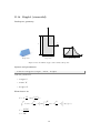
Figure B.3: A truncated pyramid with a rectangular base.
Syntax and parameters
FormFactorAnisoPyramid (length , width , height , alpha )
with the parameters
• length of the base, 𝐿,
• width of the base, 𝑊 ,
• height, 𝐻
• alpha, angle between the base and a side face, 𝛼.
They must fulfill
𝐻≤
tan 𝛼
𝐿
2
and 𝐻 ≤
tan 𝛼
𝑊
2
Form factor etc
Notation:
ℓ ≔ 𝐿/2,
𝑤 ≔ 𝑊 /2,
ℎ ≔ 𝐻/2,
𝑓± (𝑧) ≔ exp(±𝑖𝑧) sinc(𝑧).
Results:
𝐹 =
𝑞𝑥 − 𝑞𝑦
𝐻
+ 𝑞𝑧 ) ℎ) exp(−𝑖(𝑞𝑥 ℓ − 𝑞𝑦 𝑤))
{+𝑓+ ((
𝑞𝑥 𝑞𝑦
tan 𝛼
+𝑓− ((
𝑞𝑥 − 𝑞𝑦
− 𝑞𝑧 ) ℎ) exp(+𝑖(𝑞𝑥 ℓ − 𝑞𝑦 𝑤))
tan 𝛼
−𝑓+ ((
𝑞𝑥 + 𝑞𝑦
+ 𝑞𝑧 ) ℎ) exp(−𝑖(𝑞𝑥 ℓ + 𝑞𝑦 𝑤))
tan 𝛼
−𝑓− ((
𝑞𝑥 + 𝑞𝑦
− 𝑞𝑧 ) ℎ) exp(+𝑖(𝑞𝑥 ℓ + 𝑞𝑦 𝑤))},
tan 𝛼
34
𝑉 = 𝐻[𝐿𝑊 −
(𝐿 + 𝑊 )𝐻
4 𝐻2
+
].
tan 𝛼
3 tan2 𝛼
𝑆 = 𝐿𝑊 .
Examples
ω =30 ◦
8
7
6
5
4
3
2
1
00 1 2 3 4 5 6 7 8
φ f( ◦ )
ω =60 ◦
8
7
6
5
4
3
2
1
00 1 2 3 4 5 6 7 8
φ f( ◦ )
ω =90 ◦
8
7
6
5
4
3
2
1
00 1 2 3 4 5 6 7 8
φ f( ◦ )
100
10-1
10-2
10-3
10-4
10-5
10-6
10-7
/V 2
α f( ◦ )
◦
|F(q)|2
ω =0
8
7
6
5
4
3
2
1
00 1 2 3 4 5 6 7 8
φ f( ◦ )
10-8
10-9
10-10
Figure B.4: Normalized intensity |𝐹 |2 /𝑉 2 , computed with 𝐿 = 13 nm, 𝑊 = 8 nm, 𝐻 =
4.2 nm, and 𝛼 = 60∘ , for four different angles 𝜔 of rotation around the 𝑧 axis.
References
Agrees with the In-plane anisotropic pyramid form factor of IsGISAXS [7, Eq. 2.40] [8,
Eq. 217], except for different parametrization and for a refactoring of the analytical
expression for 𝐹 (𝒒). This is not the anisotropic pyramid of FitGISAXS, which is a true
pyramid with an off-center apex [14].
35
B.2
Box (cuboid)
Real-space geometry
y
z
W
x
H
x
L
Perspective
Top view
Side view
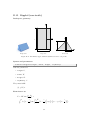
Figure B.5: A rectangular cuboid.
Syntax and parameters
FormFactorBox (length , width , height )
with the parameters
• length of the base, 𝐿,
• width of the base, 𝑊 ,
• height, 𝐻.
Form factor etc
𝐹 = 𝐿𝑊 𝐻 exp (𝑖𝑞𝑧
𝐻
𝐿
𝑊
𝐻
) sinc (𝑞𝑥 ) sinc (𝑞𝑦 ) sinc (𝑞𝑧 ) ,
2
2
2
2
𝑉 = 𝐿𝑊 𝐻,
𝑆 = 𝐿𝑊 .
Examples
ω =0 ◦
5
ω =30 ◦
5
ω =60 ◦
5
ω =90 ◦
5
100
10-1
4
4
4
4
3
3
3
3
2
2
2
2
1
1
1
1
10-2
10-5
10-6
10-7
/V 2
10-4
|F(q)|2
α f( ◦ )
10-3
10-8
10-9
00
1
2
φ f( ◦ )
3
4
5 00
1
2
φ f( ◦ )
3
4
5 00
1
2
φ f( ◦ )
3
4
5 00
1
2
φ f( ◦ )
3
4
5
10-10
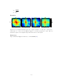
Figure B.6: Normalized intensity |𝐹 |2 /𝑉 2 , computed with 𝐿 = 18 nm, 𝑊 = 4.6 nm, and
𝐻 = 3 nm, for four different angles 𝜔 of rotation around the 𝑧 axis.
36
References
Agrees with Box form factor of IsGISAXS [7, Eq. 2.38] [8, Eq. 214], except for factors
1/2 in the definitions of parameters 𝐿, 𝑊 , 𝐻.
37
B.3
Cone (circular)
y
z
x
H
a
x
2R
Perspective
Top view
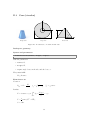
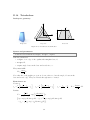
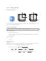
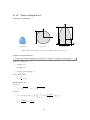
Figure B.7: A truncated cone with circular base.
Real-space geometry
Syntax and parameters
FormFactorCone (radius , height , alpha)
with the parameters
• radius, 𝑅,
• height, 𝐻,
• alpha, angle between the side and the base, 𝛼.
They must fulfill
𝐻 ≤ 𝑅 tan 𝛼.
Form factor etc
Notation:
𝑅𝐻 ≔ 𝑅 −
𝐻
,
tan 𝛼
2 + 𝑞2 ,
𝑞∥ ≔ √𝑞𝑥
𝑦
𝑞𝑧̃ ≔ 𝑞𝑧 tan 𝛼.
Results:
𝑅
𝐹 = 2𝜋 tan 𝛼 e𝑖𝑞𝑧̃ 𝑅 ∫ d𝜌 𝜌2
𝑅𝐻
𝑉 =
𝐽1 (𝑞∥ 𝜌) −𝑖𝑞 ̃ 𝜌
e 𝑧 ,
𝑞∥ 𝜌
𝜋
3
tan 𝛼 (𝑅3 − 𝑅𝐻
),
3
𝑆 = 𝜋𝑅2 .
38
Side view
Examples
ϑ =0 ◦
5
ϑ =10 ◦
5
ϑ =20 ◦
5
ϑ =30 ◦
5
100
10-1
4
4
4
4
3
3
3
3
2
2
2
2
1
1
1
1
10-2
10-5
10-6
10-7
/V 2
10-4
|F(q)|2
α f( ◦ )
10-3
10-8
10-9
00
1
2
φ f( ◦ )
3
4
5 00
1
2
φ f( ◦ )
3
4
5 00
1
2
φ f( ◦ )
3
4
5 00
1
2
φ f( ◦ )
3
4
5
10-10
Figure B.8: Normalized intensity |𝐹 |2 /𝑉 2 , computed with 𝑅 = 4 nm, 𝐻 = 11 nm, and
𝛼 = 75∘ , for four different tilt angles 𝜗 (rotation around the 𝑦 axis).
References
Agrees with Cone form factor of IsGISAXS [7, Eq. 2.28] [8, Eq. 225], except for a
substitution 𝑧 → 𝜌 in our expression for 𝐹 .
39
B.4
Cone6 (hexagonal)
Real-space geometry
y
z
x
H
b
x
R
Perspective
Top view
Side view
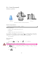
Figure B.9: A truncated hexagonal pyramid.
Syntax and parameters
FormFactorCone6 (radius ,height , alpha)
with the parameters
• radius of the regular hexagonal base, 𝑅,
• height, 𝐻,
• alpha, between the base and a side face, 𝛼.
Note that the orthographic projection does not show
√ 𝛼, but the angle 𝛽 between the
base and a side edge. They are related through 3 tan 𝛼 = 2 tan 𝛽. The following is
written more conveniently in terms of 𝛽. The parameters must fulfill
𝐻 ≤ (tan 𝛽)𝑅.
Form factor etc
Notation:
𝑅𝐻
𝐻
,
≔𝑅−
tan 𝛽
1
𝑞𝑥̃ ≔ 𝑞𝑦 ,
2
√
𝑞𝑦̃ ≔
3
𝑞 ,
2 𝑦
𝑞𝑧̃ ≔ (tan 𝛽)𝑞𝑧 .
Results:
The integral in 𝐹 could be worked out algebraically.
√ 𝑖𝑞 ̃ 𝑅 𝑅
3e 𝑧
𝐹 = 2
∫ d𝜌 e−𝑖𝑞𝑧̃ 𝜌 [𝜌𝑞𝑦̃ sinc(𝑞𝑥̃ 𝜌) sin(𝑞𝑦̃ 𝜌)+cos(2𝑞𝑥̃ 𝜌)−cos(𝑞𝑦̃ 𝜌) cos(𝑞𝑥̃ 𝜌)],
2̃
𝑞𝑦̃ − 𝑞𝑥
𝑅
𝐻
3
𝑉 = tan 𝛽 (𝑅3 − 𝑅𝐻
),
√ 2
3 3𝑅
.
𝑆=
2
40
Examples
ω =0 ◦
5
ω =10 ◦
5
ω =20 ◦
5
ω =30 ◦
5
100
10-1
4
4
4
4
3
3
3
3
2
2
2
2
1
1
1
1
10-2
10-5
10-6
10-7
/V 2
10-4
|F(q)|2
α f( ◦ )
10-3
10-8
10-9
00
1
2
φ f( ◦ )
3
4
5 00
1
2
φ f( ◦ )
3
4
5 00
1
2
φ f( ◦ )
3
4
5 00
1
2
φ f( ◦ )
3
4
5
10-10
Figure B.10: Normalized intensity |𝐹 |2 /𝑉 2 , computed with 𝑅 = 6 nm, 𝐻 = 5 nm, and
𝛼 = 60∘ , for four different angles 𝜔 of rotation around the 𝑧 axis.
References
Hopefully agrees with Cone6 form factor of IsGISAXS [7, Eq. 2.32] [8, Eq. 222], except
for different parametrization.
41
B.5
Cuboctahedron
Real-space geometry
z
y
rHH
L
x
H
x
L
Perspective
Top view
Side view
Figure B.11: A compound of two truncated pyramids with a common square base and opposite
orientations.
Syntax and parameters
FormFactorCuboctahedron (length , height , height_ratio , alpha )
with the parameters
• length of the shared square base, 𝐿,
• height of the bottom pyramid, 𝐻,
• height_ratio between the top and the bottom pyramid, 𝑟𝐻 ,
• alpha, angle between the base and a side face, 𝛼.
They must fulfill
𝐻≤
tan 𝛼
𝐿
2
and 𝑟ℎ 𝐻 ≤
tan 𝛼
𝐿.
2
Form factor etc
Using the form factor of a square pyramid 𝐹Py (Sect. B.13):
𝐹 = exp(𝑖𝑞𝑧 𝐻)[𝐹Py (𝑞𝑥 , 𝑞𝑦 , 𝑞𝑧 , 𝐿, 𝑟𝐻 𝐻, 𝛼) + 𝐹Py (𝑞𝑥 , 𝑞𝑦 , −𝑞𝑧 , 𝐿, 𝐻, 𝛼))],
𝑉 =
3
2𝐻
2𝑟𝐻 𝐻 3
1
tan(𝛼)𝐿3 [2 − (1 −
) − (1 −
) ],
6
𝐿 tan(𝛼)
𝐿 tan(𝛼)
𝑆 = 𝐿2 .
42
Examples
ω =0 ◦
5
ω =15 ◦
5
ω =30 ◦
5
ω =45 ◦
5
100
10-1
4
4
4
4
3
3
3
3
2
2
2
2
1
1
1
1
10-2
10-5
10-6
10-7
/V 2
10-4
|F(q)|2
α f( ◦ )
10-3
10-8
10-9
00
1
2
φ f( ◦ )
3
4
5 00
1
2
φ f( ◦ )
3
4
5 00
1
2
φ f( ◦ )
3
4
5 00
1
2
φ f( ◦ )
3
4
5
10-10
Figure B.12: Normalized intensity |𝐹 |2 /𝑉 2 , computed with 𝐿 = 8 nm, 𝐻 = 5 nm, 𝑟𝐻 = 0.5,
and 𝛼 = 60∘ , for four different angles 𝜔 of rotation around the 𝑧 axis.
References
Agrees with Cuboctahedron form factor of IsGISAXS [7, Eq. 2.34] [8, Eq. 218], except
for different parametrization 𝐿 = 2𝑅IsGISAXS .
43
B.6
Cylinder
Real-space geometry
y
z
2R
x
H
Perspective
Top view
Figure B.13: An upright circular cylinder.
Syntax and parameters
FormFactorCylinder (radius , height )
with the parameters
• radius of the circular base, 𝑅,
• height, 𝐻.
Form factor etc
Notation:
2 + 𝑞2 .
𝑞∥ ≔ √𝑞𝑥
𝑦
Results:
𝐹 = 2𝜋𝑅2 𝐻 sinc (𝑞𝑧
𝐻 𝐽1 (𝑞∥ 𝑅)
𝐻
) exp (𝑖𝑞𝑧 )
,
2
2
𝑞∥ 𝑅
𝑉 = 𝜋𝑅2 𝐻,
𝑆 = 𝜋𝑅2 .
44
Side view
x
Examples
ϑ =0 ◦
5
ϑ =10 ◦
5
ϑ =20 ◦
5
ϑ =30 ◦
5
100
10-1
4
4
4
4
3
3
3
3
2
2
2
2
1
1
1
1
10-2
10-5
10-6
10-7
/V 2
10-4
|F(q)|2
α f( ◦ )
10-3
10-8
10-9
00
1
2
φ f( ◦ )
3
4
5 00
1
2
φ f( ◦ )
3
4
5 00
1
2
φ f( ◦ )
3
4
5 00
1
2
φ f( ◦ )
3
4
5
10-10
Figure B.14: Normalized intensity |𝐹 |2 /𝑉 2 , computed with 𝑅 = 3 nm and 𝐻 = 8.8 nm, for
four different tilt angles 𝜗 (rotation around the 𝑦 axis).
References
Agrees with Cylinder form factor of IsGISAXS [7, Eq. 2.27] [8, Eq. 223].
45
B.7
EllipsoidalCylinder
Real-space geometry
y
z
2rb
x
H
x
2ra
Perspective
Top view
Side view
Figure B.15: A upright cylinder whose cross section is an ellipse.
Syntax and parameters
FormFactorEllipsoidalCylinder (radius_a , radius_b , height )
with the parameters
• radius_a, in 𝑥 direction, 𝑅𝑎 ,
• radius_b, in 𝑦 direction, 𝑅𝑏 ,
• height, 𝐻.
Form factor etc
Notation:
𝛾 ≔ √(𝑞𝑥 𝑅𝑎 )2 + (𝑞𝑦 𝑅𝑏 )2
Results:
𝐹 = 2𝜋𝑅𝑎 𝑅𝑏 𝐻 exp (𝑖
𝑞 𝐻 𝐽 (𝛾)
𝑞𝑧 𝐻
) sinc ( 𝑧 ) 1
,
2
2
𝛾
𝑉 = 𝜋𝑅𝑎 𝑅𝑏 𝐻,
𝑆 = 𝑅𝑎 𝑅𝑏 .
46
Examples
ω =0 ◦
5
ω =30 ◦
5
ω =60 ◦
5
ω =90 ◦
5
100
10-1
4
4
4
4
3
3
3
3
2
2
2
2
1
1
1
1
10-2
10-5
10-6
10-7
/V 2
10-4
|F(q)|2
α f( ◦ )
10-3
10-8
10-9
00
1
2
φ f( ◦ )
3
4
5 00
1
2
φ f( ◦ )
3
4
5 00
1
2
φ f( ◦ )
3
4
5 00
1
2
φ f( ◦ )
3
4
5
10-10
Figure B.16: Normalized intensity |𝐹 |2 /𝑉 2 , computed with 𝑅𝑎 = 6.3 nm, 𝑅𝑏 = 4.2 nm and
𝐻 = 3 nm, for four different angles 𝜔 of rotation around the 𝑧 axis.
References
Agrees with the IsGISAXS form factor Ellipsoid [7, Eq. 2.41, wrongly labeled in Fig. 2.4]
or Ellipsoidal Cylinder [8, Eq. 224].
47
B.8
FullSphere
Real-space geometry
y
z
2R
x
Perspective
Top view
Figure B.17: A full sphere.
Syntax and parameters
FormFactorFullSphere ( radius )
with the parameter
• radius, 𝑅.
Form factor etc
𝐹 = 4𝜋𝑅3 exp(𝑖𝑞𝑧 𝑅)
𝑉 =
sin(𝑞𝑅) − 𝑞𝑅 cos(𝑞𝑅)
,
(𝑞𝑅)3
4𝜋 3
𝑅 ,
3
𝑆 = 𝜋𝑅2 .
48
2R
Side view
x
Example
5
100
10-1
10-3
3
10-4
10-5
2
10-6
10-7
1
00
/V 2
10-2
|F(q)|2
α f( ◦ )
4
10-8
10-9
1
2 ◦3
φ f( )
4
5
10-10
Figure B.18: Normalized intensity |𝐹 |2 /𝑉 2 , computed with 𝑅 = 3.9 nm.
References
This form factor, which certainly goes back at least to Lord Rayleigh, agrees with the
Full sphere of IsGISAXS[7, Eq. 2.36] [8, Eq. 226].
49
B.9
HemiEllipsoid
Real-space geometry
y
z
2rb
x
H
x
2ra
Perspective
Top view
Side view
Figure B.19: An horizontally oriented ellipsoid, truncated at the central plane.
Syntax and parameters
FormFactorHemiEllipsoid (radius_a , radius_b , height )
with the parameters
• radius_a, in 𝑥 direction, 𝑅𝑎 ,
• radius_b, in 𝑦 direction, 𝑅𝑏 ,
• height, equal to radius in 𝑧 direction, 𝐻
Form factor etc
Notation:
𝑟𝑎,𝑧 ≔ 𝑅𝑎 √1 − (
𝑧 2
) ,
𝐻
𝑟𝑏,𝑧 ≔ 𝑅𝑏 √1 − (
Results:
𝐻
𝐹 = 2𝜋 ∫ d𝑧 𝑟𝑎,𝑧 𝑟𝑏,𝑧
0
𝐽1 (𝛾𝑧 )
exp(𝑖𝑞𝑧 𝑧),
𝛾𝑧
2
𝑉 = 𝜋𝑅𝑎 𝑅𝑏 𝐻,
3
𝑆 = 𝜋𝑅𝑎 𝑅𝑏 .
50
𝑧 2
) ,
𝐻
𝛾𝑧 = √(𝑞𝑥 𝑟𝑎,𝑧 )2 + (𝑞𝑦 𝑟𝑏,𝑧 )2 .
Examples
ω =0 ◦
5
ω =30 ◦
5
ω =60 ◦
5
ω =90 ◦
5
100
10-1
4
4
4
4
3
3
3
3
2
2
2
2
1
1
1
1
10-2
10-5
10-6
10-7
/V 2
10-4
|F(q)|2
α f( ◦ )
10-3
10-8
10-9
00
1
2
φ f( ◦ )
3
4
5 00
1
2
φ f( ◦ )
3
4
5 00
1
2
φ f( ◦ )
3
4
5 00
1
2
φ f( ◦ )
3
4
5
10-10
Figure B.20: Normalized intensity |𝐹 |2 /𝑉 2 , computed with 𝑅𝑎 = 10 nm, 𝑅𝑏 = 3.8 nm and
𝐻 = 3.2 nm, for four different angles 𝜔 of rotation around the 𝑧 axis.
References
Agrees with the IsGISAXS form factor Anisotropic hemi-ellipsoid [7, Eq. 2.42, with
wrong sign in the 𝑧-dependent phase factor] or Hemi-spheroid [8, Eq. 229].
51
B.10
FullSpheroid
Real-space geometry
z
y
H
2R
x
Perspective
Top view
Side view
Figure B.21: A full spheroid, generated by rotating an ellipse around the vertical axis.
Syntax and parameters
FormFactorFullSpheroid (radius , height )
with the parameters
• radius, 𝑅,
• height, 𝐻.
Form factor etc
Notation:
𝑅𝑧 ≔ 𝑅 √ 1 −
4𝑧2
,
𝐻2
2 + 𝑞2 .
𝑞∥ ≔ √𝑞𝑥
𝑦
Results:
𝐻/2
𝐹 = 4𝜋 exp(𝑖𝑞𝑧 𝐻/2) ∫
0
d𝑧 𝑅𝑧2
𝐽1 (𝑞∥ 𝑅𝑧 )
cos(𝑞𝑧 𝑧),
𝑞∥ 𝑅𝑧
2
𝑉 = 𝑅2 𝐻,
3
𝑆 = 𝜋𝑅2 .
52
x
Example
5
100
10-1
10-3
3
10-4
10-5
2
10-6
10-7
1
00
/V 2
10-2
|F(q)|2
α f( ◦ )
4
10-8
10-9
1
2 ◦3
φ f( )
4
5
10-10
Figure B.22: Normalized intensity |𝐹 |2 /𝑉 2 , computed with 𝑅 = 3.5 nm and 𝐻 = 9.8 nm.
References
Agrees with the Full spheroid form factor of IsGISAXS [7, Eq. 2.37] [8, Eq. 227], with
corrected volume formula. We also discovered a wrong factor of 2 in the IsGISAXS
code.
53
B.11
Prism3 (triangular)
Real-space geometry
probably the 𝑥𝑦 view needs to be rotated by 30∘
y
z
L
x
H
x
L
Perspective
Top view
Side view
Figure B.23: A prism based on an equilateral triangle.
Syntax and parameters
FormFactorPrism3 (length , height )
with the parameters
• length of one base edge, 𝐿,
• height, 𝐻.
Form factor etc
√
√
√
𝐿
𝐿
2 3
𝐿
𝐿
𝐿
√
)
−
cos
(𝑞
)
−
𝑖
𝐹 = 2
exp
(−𝑖𝑞
)
[exp
(𝑖
3𝑞
3𝑞𝑦 sinc (𝑞𝑥 )]
𝑥
𝑦
𝑦
2
𝑞𝑥 − 3𝑞𝑦
2
2
2
2
2 3
𝐻
𝐻
× 𝐻 sinc (𝑞𝑧 ) exp (𝑖𝑞𝑧 ) ,
2
2
√
𝑉 =
3
𝐻𝐿2 ,
4
√
𝑆=
3 2
𝐿 .
4
54
Examples
ω =0 ◦
5
ω =10 ◦
5
ω =20 ◦
5
ω =30 ◦
5
100
10-1
4
4
4
4
3
3
3
3
2
2
2
2
1
1
1
1
10-2
10-5
10-6
10-7
/V 2
10-4
|F(q)|2
α f( ◦ )
10-3
10-8
10-9
00
1
2
φ f( ◦ )
3
4
5 00
1
2
φ f( ◦ )
3
4
5 00
1
2
φ f( ◦ )
3
4
5 00
1
2
φ f( ◦ )
3
4
5
10-10
Figure B.24: Normalized intensity |𝐹 |2 /𝑉 2 , computed with 𝑅 = 13.8 nm and 𝐻 = 3 nm, for
four different angles 𝜔 of rotation around the 𝑧 axis.
References
Agrees with Prism3 form factor of IsGISAXS [7, Eq. 2.29] [8, Eq. 219], except for the
definition of parameter 𝐿 = 2𝑅IsGISAXS . In FitGISAXS just called Prism [14].
55
B.12
Prism6 (hexagonal)
Real-space geometry
y
R
z
x
H
Perspective
Top view
Side view
x
Figure B.25: A prism based on a regular hexagon.
Syntax and parameters
FormFactorPrism6 (radius , height )
with the parameters
• radius of the hexagonal base, 𝑅,
• height, 𝐻.
Form factor etc
√
4𝐻 3
𝐻
𝐻
𝐹 = 2
sinc (𝑞𝑧 ) exp (−𝑖𝑞𝑧 ) ×
2
3𝑞𝑦 − 𝑞𝑥
2
2
√
√
2 2
3𝑞𝑦 𝑅
3𝑞𝑦 𝑅
𝑞𝑥 𝑅
3𝑅
𝑞 𝑅
{
sinc (
) sinc (
) + cos(𝑞𝑥 𝑅) − cos (𝑞𝑦
) cos ( 𝑥 )} ,
4
2
2
2
2
√
3 3
𝑉 =
𝐻𝑅2 ,
2
√
3 3𝑅2
𝑆=
.
2
Examples
56
ω =0 ◦
5
ω =10 ◦
5
ω =20 ◦
5
ω =30 ◦
5
100
10-1
4
4
4
4
3
3
3
3
2
2
2
2
1
1
1
1
10-2
10-5
10-6
10-7
/V 2
10-4
|F(q)|2
α f( ◦ )
10-3
10-8
10-9
00
1
2
φ f( ◦ )
3
4
5 00
1
2
φ f( ◦ )
3
4
5 00
1
2
φ f( ◦ )
3
4
5 00
1
2
φ f( ◦ )
3
4
5
10-10
Figure B.26: Normalized intensity |𝐹 |2 /𝑉 2 , computed with 𝑅 = 5.7 nm and 𝐻 = 3 nm, for
four different angles 𝜔 of rotation around the 𝑧 axis.
References
Corresponds to Prism6 form factor of IsGISAXS [7, Eq. 2.31] [8, Eq. 221], which has
different parametrization and lacks a factor 𝐻 in 𝐹 (𝒒).
57
B.13
Pyramid (square-based)
Real-space geometry
y
z
L
x
H
a
x
L
Perspective
Top view
Figure B.27: A truncated pyramid with a square base.
Syntax and parameters
FormFactorPyramid (length , height , alpha )
with the parameters
• length of one edge of the square base, 𝐿,
• height, 𝐻,
• alpha, angle between the base and a side face, 𝛼,
They must fulfill
tan 𝛼
𝐿.
𝐻≤
2
Form factor etc
Notation:
ℓ ≔ 𝐿/2,
ℎ ≔ 𝐻/2,
𝑓± (𝑧) ≔ exp(±𝑖𝑧) sinc(𝑧).
Results:
𝐹 =
𝑞𝑥 − 𝑞𝑦
𝐻
+ 𝑞𝑧 ) ℎ) exp(−𝑖(𝑞𝑥 − 𝑞𝑦 )ℓ)
{+𝑓+ ((
𝑞𝑥 𝑞𝑦
tan 𝛼
+𝑓− ((
𝑞𝑥 − 𝑞𝑦
− 𝑞𝑧 ) ℎ) exp(+𝑖(𝑞𝑥 − 𝑞𝑦 )ℓ)
tan 𝛼
−𝑓+ ((
𝑞𝑥 + 𝑞𝑦
+ 𝑞𝑧 ) ℎ) exp(−𝑖(𝑞𝑥 + 𝑞𝑦 )ℓ)
tan 𝛼
−𝑓− ((
𝑞𝑥 + 𝑞𝑦
− 𝑞𝑧 ) ℎ) exp(+𝑖(𝑞𝑥 + 𝑞𝑦 )ℓ)},
tan 𝛼
58
Side view
𝑉 = 𝐻[𝐿2 −
2𝐿𝐻
4 𝐻2
+
].
tan 𝛼 3 tan2 𝛼
𝑆 = 𝐿2 .
3
2𝐻
1
𝑉 = 𝐿3 tan 𝛼 [1 − (1 −
) ],,
6
𝐿 tan 𝛼
𝑆 = 𝐿2 .
Examples
ω =0 ◦
5
ω =15 ◦
5
ω =30 ◦
5
ω =45 ◦
5
100
10-1
4
4
4
4
3
3
3
3
2
2
2
2
1
1
1
1
10-2
10-5
10-6
10-7
/V 2
10-4
|F(q)|2
α f( ◦ )
10-3
10-8
10-9
00
1
2
φ f( ◦ )
3
4
5 00
1
2
φ f( ◦ )
3
4
5 00
1
2
φ f( ◦ )
3
4
5 00
1
2
φ f( ◦ )
3
4
5
10-10
Figure B.28: Normalized intensity |𝐹 |2 /𝑉 2 , computed with 𝐿 = 10 nm, 𝐻 = 4.2 nm and
𝛼 = 60∘ , for four different angles 𝜔 of rotation around the 𝑧 axis.
References
Corresponds to Pyramid form factor of IsGISAXS [7, Eq. 2.31] [8, Eq. 221], with
different parametrization 𝐿 = 2𝑅IsGISXAXS , with correction of a sign error, and with a
more compact form of 𝐹 (𝒒).
59
B.14
Ripple1 (sinusoidal)
Real-space geometry
x
y
L
z
H
W
Perspective
Top view
W
Side view
Figure B.29: An infinite ripple with a sinusoidal profile.
Syntax and parameters
FormFactorRipple1 (length , width , height )
with the parameters
• length, 𝐿,
• width, 𝑊 ,
• height, 𝐻.
Form factor etc
𝑞 𝐿
𝑊
⋅ sinc ( 𝑥 ) ×
𝜋
2
𝐻
𝑞𝑦 𝑊
2𝑧
2𝑧
∫ d𝑧 arccos ( − 1) sinc [
arccos ( − 1)] exp (𝑖𝑞𝑧 𝑧) ,
𝐻
2𝜋
𝐻
0
𝐹 =𝐿⋅
𝑉 =
𝐿𝑊 𝐻
,
2
𝑆 = 𝐿𝑊 .
60
y
Examples
ω =0 ◦
5
ω =30 ◦
5
ω =60 ◦
5
ω =90 ◦
5
100
10-1
4
4
4
4
3
3
3
3
2
2
2
2
1
1
1
1
10-2
10-5
10-6
10-7
/V 2
10-4
|F(q)|2
α f( ◦ )
10-3
10-8
10-9
00
1
2
φ f( ◦ )
3
4
5 00
1
2
φ f( ◦ )
3
4
5 00
1
2
φ f( ◦ )
3
4
5 00
1
2
φ f( ◦ )
3
4
5
10-10
Figure B.30: Normalized intensity |𝐹 |2 /𝑉 2 , computed with 𝐿 = 25 nm, 𝑊 = 10 nm and
𝐻 = 8 nm, for four different angles 𝜔 of rotation around the 𝑧 axis.
References
Agrees with the Ripple1 form factor of FitGISAXS [14].
61
B.15
Ripple2 (saw-tooth)
Real-space geometry
x
z
d
y
L
H
y
W
Perspective
Top view
W/2
Side view
Figure B.31: An infinite ripple with an asymmetric saw-tooth profile.
Syntax and parameters
FormFactorRipple2 (length , width , height , asymmetry )
with the parameters
• length, 𝐿,
• width, 𝑊 ,
• height, 𝐻.
• asymmetry, 𝑑.
They must fulfill
|𝑑| ≤ 𝑊 /2.
Form factor etc
𝑞𝑥 𝐿
)×
2
𝐻
𝑞𝑦 𝑊
𝑧
𝑧
𝑧
∫ d𝑧 (1 − ) sinc [
(1 − )] exp {𝑖 [𝑞𝑧 𝑧 − 𝑞𝑦 𝑑 (1 − )]}
𝐻
2
𝐻
𝐻
0
𝐹 = 𝐿𝑊 sinc (
62
𝐿𝑊 𝐻
,
2
𝑆 = 𝐿𝑊 .
𝑉 =
Examples
ω =0 ◦
ω =30 ◦
ω =60 ◦
ω =90 ◦
4
4
4
4
2
2
2
2
0
0
0
0
2
2
2
2
4
4
4
4
100
10-1
10-4
10-5
10-6
10-7
/V 2
10-3
|F(q)|2
α f( ◦ )
10-2
10-8
4
2
0
φ f( ◦ )
2
4
4
2
0
φ f( ◦ )
2
4
4
2
0
φ f( ◦ )
2
4
10-9
4
2
0
φ f( ◦ )
2
4
10-10
Figure B.32: Normalized intensity |𝐹 |2 /𝑉 2 , computed with 𝐿 = 25 nm, 𝑊 = 10 nm, 𝐻 =
8 nm, and 𝑑 = 5 nm, for four different angles 𝜔 of rotation around the 𝑧 axis. The low
symmetry requires other angular ranges than used in most other figures.
References
Agrees with the Ripple2 form factor of FitGISAXS [14].
63
B.16
Tetrahedron
Real-space geometry
y
z
L
x
H
b
x
L
Perspective
Top view
Side view
Figure B.33: A truncated tetrahedron.
Syntax and parameters
FormFactorTetrahedron (length , height , alpha )
with the parameters
• length of one edge of the equilateral triangular base, 𝐿,
• height, 𝐻,
• alpha, angle between the base and a side face, 𝛼.
They must fulfill
tan 𝛼
𝐻 ≤ √ 𝐿.
2 3
Note that the orthographic projection does not show 𝛼, but the angle 𝛽 between the
base and a side edge. They are related through tan 𝛼 = 2 tan 𝛽.
Form factor etc
Notation:
√
1 𝑞𝑥 3 − 𝑞𝑦
𝑞1 ≔ [
− 𝑞𝑧 ] ,
2
tan 𝛼
Results:
√
1 𝑞𝑥 3 + 𝑞𝑦
𝑞2 ≔ [
+ 𝑞𝑧 ] ,
2
tan 𝛼
√
𝑞3 ≔
𝑞𝑦
𝑞
− 𝑧,
tan 𝛼 2
𝑞 𝐿 tan(𝛼)
3𝐻
exp (𝑖 𝑧 √
)×
2
− 3𝑞𝑦 )
2 3
√
{2𝑞𝑥 exp(𝑖𝑞3 𝐷) sinc(𝑞3 𝐻) − (𝑞𝑥 + 3𝑞𝑦 ) exp(𝑖𝑞1 𝐷) sinc(𝑞1 𝐻)
√
− (𝑞𝑥 − 3𝑞𝑦 ) exp(−𝑖𝑞2 𝐷) sinc(𝑞2 𝐻)},
𝐹 =
2
𝑞𝑥 (𝑞𝑥
64
𝐷≔
𝐿 tan 𝛼
√
−𝐻.
3
tan(𝛼)𝐿3
𝑉 =
24
√
3 2
𝑆=
𝐿 .
4
√
3
⎡1 − (1 − 2 3𝐻 ) ⎤ ,
⎢
⎥
𝐿 tan(𝛼)
⎣
⎦
Examples
ω =0 ◦
ω =20 ◦
ω =40 ◦
ω =60 ◦
4
4
4
4
2
2
2
2
0
0
0
0
2
2
2
2
4
4
4
4
100
10-1
10-4
10-5
10-6
10-7
/V 2
10-3
|F(q)|2
α f( ◦ )
10-2
10-8
4
2
0
φ f( ◦ )
2
4
4
2
0
φ f( ◦ )
2
4
4
2
0
φ f( ◦ )
2
4
10-9
4
2
0
φ f( ◦ )
2
4
10-10
Figure B.34: Normalized intensity |𝐹 |2 /𝑉 2 , computed with 𝐿 = 12 nm, 𝐻 = 8 nm, and
𝛼 = 75∘ , for four different angles 𝜔 of rotation around the 𝑧 axis. The low symmetry requires
other angular ranges than used in most other figures.
References
Agrees with the Tetrahedron form factor of IsGISAXS [7, Eq. 2.30] [8, Eq. 220]. In
FitGISAXS correctly called Truncated tetrahedron [14].
65
B.17
TruncatedCube
Real-space geometry
y
z
t
t
t
L
t
x
L
x
Perspective
L
L
Top view
Side view
Figure B.35: A cube whose eight vertices have been removed. The truncated part of each
vertex is a trirectangular tetrahedron.
Syntax and parameters
FormFactorTruncatedCube (length , removed_length )
with the parameters
• length of the full cube, 𝐿,
• removed_length, side length of the trirectangular tetrahedron removed from the
cube’s vertices, 𝑡.
They must fulfill
𝑡 ≤ 𝐿/2.
Form factor etc
Notation:
Besides the form factor 𝐹Box (𝒒) of the full cube of side length 𝐿 (Sect. B.2), we need
the form factor of a trirectangular tetrahedrons as cut from the cube:
𝑞𝑥 (𝐿 − 𝑡) + 𝑞𝑦 𝐿
𝑡
)
exp (𝑖
𝑞𝑧
2
𝑞𝑦 𝑡
(𝑞𝑥 − 𝑞𝑦 )𝑡
1
𝑞𝑧
𝑞 𝑡
×{ sinc ( 𝑥 ) −
exp (𝑖
) sinc (
)
𝑞𝑦
2
𝑞𝑦 (𝑞𝑦 + 𝑞𝑧 )
2
2
𝐹vertex1 (𝑞𝑥 , 𝑞𝑦 , 𝑞𝑧 , 𝐿, 𝑡) =
−
1
(𝑞 + 𝑞𝑧 )𝑡
𝑞 𝑡
)}
exp (𝑖 𝑧 ) sinc ( 𝑥
𝑞𝑦 + 𝑞𝑧
2
2
66
Thanks to symmetry (see the following figure, which shows the vertices 𝑉𝑖 for 𝑖 =
1, … , 8), the form factors of other seven tetrahedrons cut from the cube can be computed as follows (note that the origin is taken as usual at the centre of the bottom face
of the cube):
𝐹vertex2 (𝑞𝑥 , 𝑞𝑦 , 𝑞𝑧 , 𝐿, 𝑡) = 𝐹vertex1 (𝑞𝑦 , −𝑞𝑥 , 𝑞𝑧 , 𝐿, 𝑡)
𝐹vertex3 (𝑞𝑥 , 𝑞𝑦 , 𝑞𝑧 , 𝐿, 𝑡) = 𝐹vertex1 (−𝑞𝑥 , −𝑞𝑦 , 𝑞𝑧 , 𝐿, 𝑡)
𝐹vertex4 (𝑞𝑥 , 𝑞𝑦 , 𝑞𝑧 , 𝐿, 𝑡) = 𝐹vertex1 (−𝑞𝑦 , 𝑞𝑥 , 𝑞𝑧 , 𝐿, 𝑡)
𝐹vertex5 (𝑞𝑥 , 𝑞𝑦 , 𝑞𝑧 , 𝐿, 𝑡) = exp(𝑖𝑞𝑧 𝐿)𝐹vertex1 (𝑞𝑥 , 𝑞𝑦 , −𝑞𝑧 , 𝐿, 𝑡)
𝐹vertex6 (𝑞𝑥 , 𝑞𝑦 , 𝑞𝑧 , 𝐿, 𝑡) = exp(𝑖𝑞𝑧 𝐿)𝐹vertex1 (𝑞𝑦 , −𝑞𝑥 , −𝑞𝑧 , 𝐿, 𝑡)
𝐹vertex7 (𝑞𝑥 , 𝑞𝑦 , 𝑞𝑧 , 𝐿, 𝑡) = exp(𝑖𝑞𝑧 𝐿)𝐹vertex1 (−𝑞𝑥 , −𝑞𝑦 , −𝑞𝑧 , 𝐿, 𝑡)
𝐹vertex8 (𝑞𝑥 , 𝑞𝑦 , 𝑞𝑧 , 𝐿, 𝑡) = exp(𝑖𝑞𝑧 𝐿)𝐹vertex1 (−𝑞𝑦 , 𝑞𝑥 , −𝑞𝑧 , 𝐿, 𝑡)
Result:
8
𝐹 = 𝐹Box (𝑞𝑥 , 𝑞𝑦 , 𝑞𝑧 , 𝐿, 𝐿, 𝐿) − ∑ 𝐹vertex𝑖 (𝑞𝑥 , 𝑞𝑦 , 𝑞𝑧 , 𝐿, 𝑡)
𝑖=1
4
𝑉 = 𝐿 3 − 𝑡3 ,
3
𝑆 = 𝐿2 .
Examples
67
ω =0 ◦
5
ω =15 ◦
5
ω =30 ◦
5
ω =45 ◦
5
100
10-1
4
4
4
4
3
3
3
3
2
2
2
2
1
1
1
1
10-2
10-5
10-6
10-7
/V 2
10-4
|F(q)|2
α f( ◦ )
10-3
10-8
10-9
00
1
2
φ f( ◦ )
3
4
5 00
1
2
φ f( ◦ )
3
4
5 00
1
2
φ f( ◦ )
3
4
5 00
1
2
φ f( ◦ )
3
4
5
10-10
Figure B.36: Normalized intensity |𝐹 |2 /𝑉 2 , computed with 𝐿 = 25 nm, 𝑊 = 10 nm, 𝐻 =
8 nm, and 𝑑 = 5 nm, for four different angles 𝜔 of rotation around the 𝑧 axis.
References
[15]
68
Page intentionally left blank
69
B.18
TruncatedSphere
Real-space geometry
y
z
2R
x
H
Perspective
Top view
Figure B.37: A truncated sphere.
Syntax and parameters
FormFactorTruncatedSphere (radius , height )
with the parameters
• radius, 𝑅,
• height, 𝐻.
They must fulfill
0 < 𝐻 ≤ 2𝑅.
Form factor etc
Notation:
2 + 𝑞2 ,
𝑞∥ ≔ √𝑞𝑥
𝑦
𝑅𝑧 ≔
√
𝑅2 − 𝑧2 .
Results:
𝑅
𝐹 = 2𝜋 exp[𝑖𝑞𝑧 (𝐻 − 𝑅)] ∫
d𝑧 𝑅𝑧2
𝑅−𝐻
𝐽1 (𝑞∥ 𝑅𝑧 )
exp(𝑖𝑞𝑧 𝑧)𝑑𝑧,
𝑞∥ 𝑅𝑧
2 𝐻 −𝑅 1 𝐻 −𝑅 3
− (
) ],
𝑉 = 𝜋𝑅3 [ +
3
𝑅
3
𝑅
𝑆={
𝜋𝑅2 ,
𝐻≥𝑅
2
𝜋 (2𝑅𝐻 − 𝐻 ) , 𝐻 < 𝑅
.
70
Side view
x
Example
ϑ =0 ◦
5
ϑ =10 ◦
5
ϑ =20 ◦
5
ϑ =30 ◦
5
100
10-1
4
4
4
4
3
3
3
3
2
2
2
2
1
1
1
1
10-2
10-5
10-6
10-7
/V 2
10-4
|F(q)|2
α f( ◦ )
10-3
10-8
10-9
00
1
2
φ f( ◦ )
3
4
5 00
1
2
φ f( ◦ )
3
4
5 00
1
2
φ f( ◦ )
3
4
5 00
1
2
φ f( ◦ )
3
4
5
10-10
Figure B.38: Normalized intensity |𝐹 |2 /𝑉 2 , computed with 𝑅 = 4.2 nm and 𝐻 = 6.1 nm,
for four different tilt angles 𝜗 (rotation around the 𝑦 axis).
References
Agrees with the IsGISAXS form factor Sphere [7, Eq. 2.33] or Truncated sphere [8,
Eq. 228].
71
B.19
TruncatedSpheroid
Real-space geometry
z
y
fpR
H
2R
x
x
2R
Perspective
Top view
Side view
Figure B.39: A vertically oriented, horizontally truncated spheroid.
Syntax and parameters
FormFactorTruncatedSpheroid (radius , height , height_flattening )
with the parameters
• radius, 𝑅,
• height, 𝐻.
• height_flattening, 𝑓𝑝 .
They must fulfill
0<
𝐻
≤ 2𝑓𝑝 .
𝑅
Form factor etc
Notation:
2 + 𝑞2 ,
𝑞∥ ≔ √𝑞𝑥
𝑦
𝑅𝑧 ≔ √𝑅2 − 𝑧 2 /𝑓𝑝2 .
Results:
𝑓𝑝 𝑅
𝐹 = 2𝜋 exp[𝑖𝑞𝑧 (𝐻 − 𝑓𝑝 𝑅)] ∫
d𝑧 𝑅𝑧2
𝑓𝑝 𝑅−𝐻
𝑉 =
𝜋𝑅𝐻 2
𝐻
),
(1 −
𝑓𝑝
3𝑓𝑝 𝑅
72
𝐽1 (𝑞∥ 𝑅𝑧 )
exp(𝑖𝑞𝑧 𝑧)
𝑞∥ 𝑅𝑧
⎧ 𝜋𝑅2 ,
𝐻 ≥ 𝑓𝑝 𝑅
{
2
𝑆=
.
2𝑅𝐻
𝐻
⎨ 𝜋(
− 2 ), 𝐻 < 𝑅
{
𝑓𝑝
𝑓𝑝
⎩
Example
ϑ =0 ◦
5
ϑ =10 ◦
5
ϑ =20 ◦
5
ϑ =30 ◦
5
100
10-1
4
4
4
4
3
3
3
3
2
2
2
2
1
1
1
1
10-2
10-5
10-6
10-7
/V 2
10-4
|F(q)|2
α f( ◦ )
10-3
10-8
10-9
00
1
2
φ f( ◦ )
3
4
5 00
1
2
φ f( ◦ )
3
4
5 00
1
2
φ f( ◦ )
3
4
5 00
1
2
φ f( ◦ )
3
4
5
10-10
Figure B.40: Normalized intensity |𝐹 |2 /𝑉 2 , computed with 𝑅 = 3.3 nm, 𝐻 = 9.8 nm, and
𝑓𝑝 = 1.8, for four different tilt angles 𝜗 (rotation around the 𝑦 axis).
References
Agrees with the IsGISAXS form factor Sphere [7, Eq. 2.33] or TruncatedSpheroid [8,
Eq. 228].
73
Bibliography
[1] MARIA. Magnetic reflectometer with high incident angle. http://www.
mlz-garching.de/maria.
[2] NREX. Neutron reflectometer with X-ray option. http://www.mlz-garching.
de/nrex.
[3] REFSANS. Horizontal TOF Reflectometer with GISANS option. http://www.
mlz-garching.de/refsans.
[4] High Data Rate Processing and Analysis Initiative (HDRI) of the Helmholtz Association of German research centres. http://www.pni-hdri.de.
[5] SINE2020: world-class Science and Innovation with Neutrons in Europe in 2020.
http://cordis.europa.eu/news/rcn/124015_en.html.
[6] R. Lazzari, J. Appl. Cryst. 35, 406 (2002).
[7] R. Lazzari, IsGISAXS manual, version 2.6, http://www.insp.jussieu.fr/
oxydes/IsGISAXS/figures/doc/manual.html [as per May 2015].
[8] G. Renaud, R. Lazzari and F. Leroy, Surface Science Reports 64, 255 (2009).
[9] V. P. Sears, Neutron Optics, Oxford University Press: Oxford (1989).
[10] M. Lax, Rev. Mod. Phys. 23, 287 (1951).
[11] M. Born and E. Wolf, Principles of Optics, Cambridge University Press: Cambridge (7 1999).
[12] E. Hecht, Optics, Addison Wesley: San Francisco (4 2002).
[13] M. Abramowitz and I. Stegun, Handbook of Mathematical Functions, National
Bureau of Standards (1964).
[14] D. Babonneau, FitGISAXS manual, version May 2013, http://www.pprime.fr/
sites/default/files/pictures/d1/FINANO/FitGISAXS_130531.zip [as per
May 2015].
[15] R. W. Hendricks, J. Schelten and W. Schmatz, Philos. Mag. 30, 819 (1974).
74
List of Symbols
≔
Defines what is on the left, page 7
≕
Defines what is on the right, page 7
≡
Equal as result of a definition, page 7
≃
Asymptotically equal: equal in an implied limit, page 7
≐
Equal up to first order of a power-law expansion, hence a special case
of asymptotic equality, page 7
⟨… | … | …⟩
Matrix element, defined as a volume integral, page 14
±
Upward (+) or downward (−) propagating, page 19
𝛼f
Glancing angle of the detected beam, page 17
𝛼i
Glancing angle of the incident beam, page 17
𝛽
Imaginary part of the refractive index, page 19
𝛿
Small parameter in the refractive index 𝑛 = 1 − 𝛿 + 𝑖𝛽, page 19
𝜌𝑠 (𝒓)
Scattering length density, page 11
𝜎
Scattering or absorption cross section, page 15
𝜙(𝑧)
𝑧-dependent factor of 𝜓(𝒓), page 17
𝜙f
Angle between the detected beam, projected into the sample plane, and
the 𝑥 axis, page 17
𝜙i
Angle between the incident beam, projected into the sample plane, and
the 𝑥 axis, page 17
𝜒(𝒒)
Fourier transform of the perturbation potential 𝜒(𝒓), page 14
𝜒(𝒓)
Perturbative potential, for neutrons equal to the scattering-length density 𝜌𝑠 , page 12
𝜒𝑙 (𝒒)
Fourier transform of the perturbation potential 𝜒(𝒓), evaluated in one
sample layer, page 23
75
𝜓(𝒓)
Stationary wavefunction, page 10
𝜓(𝒓, 𝑡)
Microscopic neutron wavefunction, page 10
𝜓(𝒓, 𝑡)
Coherent wavefunction, page 11
𝜓f (𝒓)
Plane wave propagating from the sample towards the detector, page 14
𝜓i (𝒓)
Incident wavefunction, page 12
𝜓s (𝒓)
Scattered wavefunction, page 13
𝜓s,far (𝒓)
Far-field approximation to the scattered wavefunction 𝜓s (𝒓), page 14
𝜓± (𝒓)
Upward (+) or downward (−) propagating component of 𝜓(𝒓), page 19
𝜔
Frequency of incident radiation, page 10
Ω
Solid angle, page 15
𝐴±
𝑤𝑙
±
Amplitude of the plane wave 𝜙𝑤𝑙
(𝒓), page 22
𝐵(𝒓, 𝒓′ )
Green function, adjoint of 𝐺, page 18
f
Subscript “final”, for outgoing waves scattered into the direction of the
detector, page 14
𝐺(𝒓, 𝒓′ )
Green function, page 13
𝐺far (𝒓, 𝒓′ )
Far-field approximation to the Green function 𝐺(𝒓, 𝒓′ ), page 14
i
Subscript “incident”, page 12
𝐽1
Bessel function of first kind and first order, page 32
𝑱(𝒓)
Probability flux, page 15
𝑘⟂
Component of 𝒌 along the sample normal, page 17
𝒌
wavevector, page 14
𝒌∥
Projection of 𝒌 onto the sample plane, page 17
𝒌±
𝑤𝑙
±
wavevector of the plane wave 𝜓𝑤𝑙
(𝒓), page 21
𝐾
Vacuum wavenumber, corresponding to the frequency 𝜔, page 11
𝑙
Index of layer in multilayer sample, page 21
𝑚
Neutron mass, page 11
𝑛(𝒓)
Refractive index, page 11
𝑛2 (𝑧)
Refractive index, horizontally averaged, page 16
76
𝒒
Scattering vector, page 14
𝒓
Position, page 10
𝒓D
Position of the detector, page 18
𝑅𝑤𝑙
Partial amplitude of 𝜓𝑤 (𝒓) in layer 𝑙 in upward (reflection) direction,
also denoted 𝐴+
𝑤𝑙 , page 22
s
Subscript “scattered”, page 13
sinc
Cardinal sine, sinc(𝑥) ≔ sin(𝑥)/𝑥, page 7
𝑆
Maximum horizontal section of embedded particle, page 32
𝑡
Time, page 10
𝑇𝑤𝑙
Partial amplitude of 𝜓𝑤 (𝒓) in layer 𝑙 in downward (transmission) direction, also denoted 𝐴−
𝑤𝑙 , page 22
𝑣(𝒓)
Macrosopic optical potential, page 11
𝑉 (𝒓)
Microscopic optical potential, page 11
𝑤
An index that can take the values i (incident) or f (final), page 19
𝑥
Horizontal coordinate, usually chosen along the incoming beam projection, page 17
𝑦
Horizontal oordinate, chosen normal to 𝑧 and 𝑥, page 17
𝑧𝑙
Vertical coordinate at the top of layer 𝑙 (at the bottom for 𝑙 = 0),
page 22
𝑧
Vertical coordinate, along the sample normal, page 16
𝒛̂
Unit vector along the sample normal, page 21
77
Index
Absorption, 19–20
Anisotropic pyramid (form factor), 34
API, see Application programming
interface
Application programming interface, 9
DWBA, see Distorted-wave Born
approximation
Ellipsoid (form factor)
truncated, 50
Ellipsoidal cylinder (form factor), 46
Evanescent wave, 26
Born approximation, 12–13
Box (form factor), 36
Bragg scattering
by atomic lattices, 11
Bug reports, 6
Facetted cube (form factor), 66
Far-field approximation, 13–14, 18
Fermi’s pseudopotential, 11
Flux
incident and scattered, 15
Form factor, 73
FormFactorAnisoPyramid, 34
FormFactorBox, 36
FormFactorCone, 38
FormFactorCone6, 40
FormFactorCuboctahedron, 42
FormFactorCylinder, 44
FormFactorEllipsoidalCylinder, 46
FormFactorFullSphere, 48
FormFactorFullSpheroid, 52
FormFactorHemiEllipsoid, 50
FormFactorPrism3, 54
FormFactorPrism6, 56
FormFactorPyramid, 58
FormFactorRipple1, 60
FormFactorRipple2, 62
FormFactorTetrahedron, 64
FormFactorTruncatedCube, 66
FormFactorTruncatedSphere, 70
FormFactorTruncatedSpheroid, 72
Forum, 9
Fraunhofer approximation, 13
Fresnel coefficients, 18, 23
Full sphere (form factor), 48
Full spheroid (form factor), 52
C++, 9
Citation, 5
Coherent forward scattering, 11
Coherent wavefunction, 11
Cone (form factor)
circular, 38
hexagonal (Cone6), 40
Continuum approximation
neutron propagation, 11
Conventions, see Sign convention, see
Horizontal and Vertical
Coordinate system, 14
Cross section, 15
Cube (form factor)
facetted, 66
Cuboctahedron (form factor), 42
Cuboid (form factor), 36
Cylinder (form factor), 44
ellipsoidal, 46
Detector
mapping the cross section, 6
transmission geometry, 25
Dissipation, 26
Distorted-wave Born approximation, 5,
18–19
multilayer, 22
Download, 8
Glancing angle, 16
78
Green function
homogeneous material, 13, 14
reciprocity, 28
vertically structured material, 18
propagation and magnetic scattering,
6
Potential, see Optical potential, see
Perturbation
Prism (form factor)
hexagonal (Prism6), 56
reactangular (Box), 36
triangular (Prism3), 54
Pyramid (form factor)
hexagonal (Cone6), 40
rectangular (AnisoPyramid), 34
square, 58
Python, 9
Helmholtz equation, 12
Hemi ellipsoid (form factor), 50
Hole, 27
Horizontal plane, 16
Huygens’ principle, 11
Inclusion, 27
Index of refraction, see Refractive index
Installation, 8
IsGISAXS, 6
Island, 27
Quadrature, 32
Reciprocity, 18, 28–29
Reflection, 16, see also Fresnel coefficients
Refraction, 16
Snell’s law, 22
Refractive index, 11
graded, 18
sign convention, 11, 19
Registration, 9
Ripple (form factor)
saw-tooth (Ripple2), 62
sinusoidal (Ripple1), 60
Roughness, 6
Layer
coordinate, 22
index, 21, 22
transfer matrix, 24
Layer structures, see Multilayer
Lazzari, Rémi, 6
Linux, 8
Lippmann-Schwinger equation, 13
MacOS, 8
Mesoparticles, see Particles
Microsoft Windows, 8
Momentum transfer, see Scattering vector
Multilayer, 21–26
coordinates, 22
numbering, 21, 22
transfer matrix, 24
Sample normal, 16
Sample plane, 16
SAS, see Small-angle scattering
Saw-tooth ripple (form factor), 62
Scattering length density, 11
Scattering vector, 14
Schrödinger equation
macroscopic, 11
microscopic, 10
Semiclassical approximation, see WKB
method
Shape transform, 73
Sign convention, 20
scattering vector, 14
wave propagation, 10
Sinusoidal ripple (form factor), 60
Small-angle scattering, 10–12
Snell’s law, 22
Sphere (form factor), 48
truncated, 70
Spheroid (form factor), 52
truncated, 72
Nanoparticles, see Particles
Neutrons
polarization, 6
wave propagation, 10–12
Newsletter, 9
Operating system, 8
Optical potential
Fourier transform, 14
macroscopic, 11
nuclear (microscopic), 11
Particle assemblies, 6, 27
Perturbation, 12
Phase integral method, see WKB method
Platform (operating system), 8
Polarized neutron
79
Tetrahedron (form factor), 64
Total reflection, 26
Transfer matrix, 24
Transition matrix, 14
Transmission, see Fresnel coefficients
Transmission geometry, 25
Truncated cone (form factor), 38
Truncated ellipsoid (form factor), 50
Truncated pyramid (form factor)
hexagonal (Cone6), 40
rectangular (AnisoPyramid), 34
square, 58
Truncated sphere (form factor), 70
Truncated spheroid (form factor), 72
Truncated tetrahedron (form factor), 64
Tunneling, 26
Tutorials, 9
Vertical direction, 16
Wave propagation, see also Sign
convention
coherent, 11
neutrons, 10–12
neutrons, polarized, 6
X-rays, 6
Wavevector
complex, 26
Windows, see Microsoft Windows
WKB method, 18
X-rays
propagation and scattering, 6
80