1
MuPAD®
User's Guide
R2015b
How to Contact MathWorks
Latest news:
www.mathworks.com
Sales and services:
www.mathworks.com/sales_and_services
User community:
www.mathworks.com/matlabcentral
Technical support:
www.mathworks.com/support/contact_us
Phone:
508-647-7000
The MathWorks, Inc.
3 Apple Hill Drive
Natick, MA 01760-2098
MuPAD® User's Guide
© COPYRIGHT 1993–2015 by SciFace Software GmbH & Co. KG.
The software described in this document is furnished under a license agreement. The software may be used
or copied only under the terms of the license agreement. No part of this manual may be photocopied or
reproduced in any form without prior written consent from The MathWorks, Inc.
FEDERAL ACQUISITION: This provision applies to all acquisitions of the Program and Documentation
by, for, or through the federal government of the United States. By accepting delivery of the Program
or Documentation, the government hereby agrees that this software or documentation qualifies as
commercial computer software or commercial computer software documentation as such terms are used
or defined in FAR 12.212, DFARS Part 227.72, and DFARS 252.227-7014. Accordingly, the terms and
conditions of this Agreement and only those rights specified in this Agreement, shall pertain to and
govern the use, modification, reproduction, release, performance, display, and disclosure of the Program
and Documentation by the federal government (or other entity acquiring for or through the federal
government) and shall supersede any conflicting contractual terms or conditions. If this License fails
to meet the government's needs or is inconsistent in any respect with federal procurement law, the
government agrees to return the Program and Documentation, unused, to The MathWorks, Inc.
Trademarks
MuPAD is a registered trademark of SciFace Software GmbH & Co. KG.
MATLAB and Simulink are registered trademarks of The MathWorks, Inc. See
www.mathworks.com/trademarks for a list of additional trademarks. Other product or brand
names may be trademarks or registered trademarks of their respective holders.
Patents
MathWorks products are protected by one or more U.S. patents. Please see
www.mathworks.com/patents for more information.
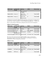
Revision History
September 2012
March 2013
September 2013
March 2014
October 2014
March 2015
September 2015
Online only
Online only
Online only
Online only
Online only
Online only
Online only
New for Version 5.9 (Release 2012b)
Revised for Version 5.10 (Release 2013a)
Revised for Version 5.11 (Release 2013b)
Revised for Version 6.0 (Release 2014a)
Revised for Version 6.1 (Release 2014b)
Revised for Version 6.2 (Release 2015a)
Revised for Version 6.3 (Release 2015b)
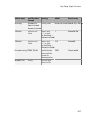
Contents
1
Getting Started
Desktop Overview . . . . . . . . . . . . . . . . . . . . . . . . . . . . . . . . . . .
1-2
Evaluate Mathematical Expressions and Commands . . . . . .
Working in a Single Input Region . . . . . . . . . . . . . . . . . . . . .
Working with Multiple Input Regions . . . . . . . . . . . . . . . . . .
1-4
1-4
1-5
Shortcut to Access Standard MuPAD Functions . . . . . . . . . .
1-7
Access Help for Particular Command . . . . . . . . . . . . . . . . . .
Autocomplete Commands . . . . . . . . . . . . . . . . . . . . . . . . . .
Use Tooltips and the Context Menu . . . . . . . . . . . . . . . . . .
Use Help Commands . . . . . . . . . . . . . . . . . . . . . . . . . . . . . .
1-15
1-15
1-16
1-18
Perform Computations . . . . . . . . . . . . . . . . . . . . . . . . . . . . . .
Compute with Numbers . . . . . . . . . . . . . . . . . . . . . . . . . . .
Differentiation . . . . . . . . . . . . . . . . . . . . . . . . . . . . . . . . . . .
Integration . . . . . . . . . . . . . . . . . . . . . . . . . . . . . . . . . . . . .
Linear Algebra . . . . . . . . . . . . . . . . . . . . . . . . . . . . . . . . . .
Solve Equations . . . . . . . . . . . . . . . . . . . . . . . . . . . . . . . . . .
Manipulate Expressions . . . . . . . . . . . . . . . . . . . . . . . . . . .
Use Assumptions in Your Computations . . . . . . . . . . . . . . .
1-19
1-19
1-23
1-26
1-27
1-31
1-33
1-36
Use Graphics . . . . . . . . . . . . . . . . . . . . . . . . . . . . . . . . . . . . . .
Graphic Options Available in MuPAD . . . . . . . . . . . . . . . . .
Basic Plotting . . . . . . . . . . . . . . . . . . . . . . . . . . . . . . . . . . .
Format Plots . . . . . . . . . . . . . . . . . . . . . . . . . . . . . . . . . . . .
Present Graphics . . . . . . . . . . . . . . . . . . . . . . . . . . . . . . . . .
Create Animated Graphics . . . . . . . . . . . . . . . . . . . . . . . . .
1-39
1-39
1-40
1-49
1-56
1-59
Use the MuPAD Libraries . . . . . . . . . . . . . . . . . . . . . . . . . . . .
Overview of Libraries . . . . . . . . . . . . . . . . . . . . . . . . . . . . .
Standard Library . . . . . . . . . . . . . . . . . . . . . . . . . . . . . . . .
1-62
1-62
1-63
iii
Find Information About a Library . . . . . . . . . . . . . . . . . . . .
Avoid Name Conflicts Between MuPAD Objects and Library
Functions . . . . . . . . . . . . . . . . . . . . . . . . . . . . . . . . . . . . .
2
iv
Contents
1-64
1-65
Notebook Interface
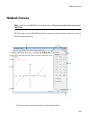
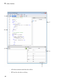
Notebook Overview . . . . . . . . . . . . . . . . . . . . . . . . . . . . . . . . . .
2-3
Debugger Window Overview . . . . . . . . . . . . . . . . . . . . . . . . . .
2-5
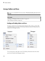
Arrange Toolbars and Panes . . . . . . . . . . . . . . . . . . . . . . . . . .
Enabling and Disabling Toolbars and Panes . . . . . . . . . . . . .
Move Toolbars and Panes . . . . . . . . . . . . . . . . . . . . . . . . . . .
2-8
2-8
2-9
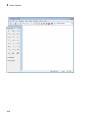
Enter Data and View Results . . . . . . . . . . . . . . . . . . . . . . . . .
2-11
View Status Information . . . . . . . . . . . . . . . . . . . . . . . . . . . . .
2-13
Save Custom Arrangements . . . . . . . . . . . . . . . . . . . . . . . . . .
2-14
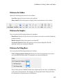
Format Text . . . . . . . . . . . . . . . . . . . . . . . . . . . . . . . . . . . . . . .
Choose Font Style, Size, and Colors . . . . . . . . . . . . . . . . . .
Choose Indention, Spacing, and Alignment . . . . . . . . . . . . .
2-15
2-15
2-18
Format Mathematical Expressions . . . . . . . . . . . . . . . . . . . .
2-21
Format Expressions in Input Regions . . . . . . . . . . . . . . . . .
2-24
Change Default Format Settings . . . . . . . . . . . . . . . . . . . . . .
2-28
Use Frames . . . . . . . . . . . . . . . . . . . . . . . . . . . . . . . . . . . . . . . .
2-32
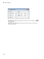
Use Tables . . . . . . . . . . . . . . . . . . . . . . . . . . . . . . . . . . . . . . . . .
Create Tables . . . . . . . . . . . . . . . . . . . . . . . . . . . . . . . . . . .
Add and Delete Rows and Columns . . . . . . . . . . . . . . . . . . .
Format Tables . . . . . . . . . . . . . . . . . . . . . . . . . . . . . . . . . . .
2-38
2-38
2-40
2-41
Embed Graphics . . . . . . . . . . . . . . . . . . . . . . . . . . . . . . . . . . . .
2-45
Work with Links . . . . . . . . . . . . . . . . . . . . . . . . . . . . . . . . . . .
Insert Links to Targets in Notebooks . . . . . . . . . . . . . . . . .
Insert Links Interactively . . . . . . . . . . . . . . . . . . . . . . . . . .
Insert Links to Arbitrary Files . . . . . . . . . . . . . . . . . . . . . .
Insert Links to Internet Addresses . . . . . . . . . . . . . . . . . . .
Edit Existing Links . . . . . . . . . . . . . . . . . . . . . . . . . . . . . . .
Delete Links . . . . . . . . . . . . . . . . . . . . . . . . . . . . . . . . . . . .
Delete Link Targets . . . . . . . . . . . . . . . . . . . . . . . . . . . . . .
2-48
2-48
2-51
2-53
2-54
2-56
2-57
2-58
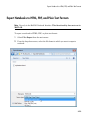
Export Notebooks to HTML, PDF, and Plain Text Formats
2-59
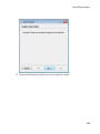
Save and Export Graphics . . . . . . . . . . . . . . . . . . . . . . . . . . .
Export Static Plots . . . . . . . . . . . . . . . . . . . . . . . . . . . . . . .
Choose the Export Format . . . . . . . . . . . . . . . . . . . . . . . . .
Save Animations . . . . . . . . . . . . . . . . . . . . . . . . . . . . . . . . .
Export Sequence of Static Images . . . . . . . . . . . . . . . . . . . .
2-61
2-61
2-64
2-65
2-66
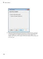
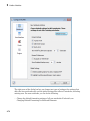
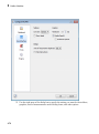
Set Preferences for Notebooks . . . . . . . . . . . . . . . . . . . . . . . .
Preferences Available for Notebooks . . . . . . . . . . . . . . . . . .
Change Default Formatting . . . . . . . . . . . . . . . . . . . . . . . .
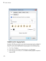
Scalable Format for Copying Graphics . . . . . . . . . . . . . . . .
2-71
2-71
2-73
2-74
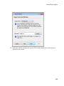
Set Preferences for Dialogs, Toolbars, and Graphics . . . . .
Preferences Available for Dialogs, Toolbars, and Graphics . .
Preferences for Toolbars . . . . . . . . . . . . . . . . . . . . . . . . . . .
Preferences for Graphics . . . . . . . . . . . . . . . . . . . . . . . . . . .
Preferences for Dialog Boxes . . . . . . . . . . . . . . . . . . . . . . . .
2-75
2-75
2-77
2-77
2-77
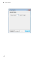
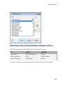
Set Font Preferences . . . . . . . . . . . . . . . . . . . . . . . . . . . . . . . .
Select Generic Fonts . . . . . . . . . . . . . . . . . . . . . . . . . . . . . .
Default Generic Fonts for Microsoft Windows, Macintosh, and
Linux . . . . . . . . . . . . . . . . . . . . . . . . . . . . . . . . . . . . . . . .
2-79
2-79
Set Engine Preferences . . . . . . . . . . . . . . . . . . . . . . . . . . . . . .
Change Global Settings . . . . . . . . . . . . . . . . . . . . . . . . . . . .
Restore Default Global Settings . . . . . . . . . . . . . . . . . . . . .
Add Hidden Startup Commands to All Notebooks . . . . . . . .
Options Available for MuPAD Engine Startup . . . . . . . . . .
2-82
2-82
2-84
2-84
2-84
Get Version Information . . . . . . . . . . . . . . . . . . . . . . . . . . . . .
2-86
Use Different Output Modes . . . . . . . . . . . . . . . . . . . . . . . . .
Abbreviations . . . . . . . . . . . . . . . . . . . . . . . . . . . . . . . . . . .
2-87
2-87
2-81
v
vi
Contents
Typeset Math Mode . . . . . . . . . . . . . . . . . . . . . . . . . . . . . . .
Pretty Print Mode . . . . . . . . . . . . . . . . . . . . . . . . . . . . . . . .
Mathematical Notations Used in Typeset Mode . . . . . . . . . .
2-88
2-90
2-92
Set Line Length in Plain Text Outputs . . . . . . . . . . . . . . . . .
2-94
Delete Outputs . . . . . . . . . . . . . . . . . . . . . . . . . . . . . . . . . . . . .
2-95
Greek Letters in Text Regions in MuPAD . . . . . . . . . . . . . .
2-96
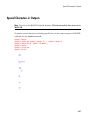
Special Characters in Outputs . . . . . . . . . . . . . . . . . . . . . . . .
2-97
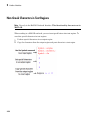
Non-Greek Characters in Text Regions . . . . . . . . . . . . . . . .
2-98
Use Keyboard Shortcuts . . . . . . . . . . . . . . . . . . . . . . . . . . . . .
2-99
Use Mnemonics . . . . . . . . . . . . . . . . . . . . . . . . . . . . . . . . . . . .
2-101
Wrap Long Lines . . . . . . . . . . . . . . . . . . . . . . . . . . . . . . . . . .
Wrap Text . . . . . . . . . . . . . . . . . . . . . . . . . . . . . . . . . . . . .
Wrap Expressions in Input Regions . . . . . . . . . . . . . . . . .
Wrap Output Expressions . . . . . . . . . . . . . . . . . . . . . . . . .
2-102
2-102
2-104
2-106
Hide Code Lines . . . . . . . . . . . . . . . . . . . . . . . . . . . . . . . . . . .
2-110
Change Font Size Quickly . . . . . . . . . . . . . . . . . . . . . . . . . .
2-113
Scale Graphics . . . . . . . . . . . . . . . . . . . . . . . . . . . . . . . . . . . .
2-116
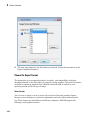
Use Print Preview . . . . . . . . . . . . . . . . . . . . . . . . . . . . . . . . .
View Documents Before Printing . . . . . . . . . . . . . . . . . . . .
Print Documents from Print Preview . . . . . . . . . . . . . . . .
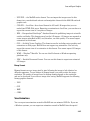
Save Documents to PDF Format . . . . . . . . . . . . . . . . . . . .
Get More Out of Print Preview . . . . . . . . . . . . . . . . . . . . .
2-118
2-118
2-118
2-119
2-120
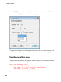
Change Page Settings for Printing . . . . . . . . . . . . . . . . . . .
2-122
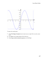
Print Wide Notebooks . . . . . . . . . . . . . . . . . . . . . . . . . . . . . .
2-123
3
Mathematics
Evaluations in Symbolic Computations . . . . . . . . . . . . . . . . .
3-5
Level of Evaluation . . . . . . . . . . . . . . . . . . . . . . . . . . . . . . . . . .
What Is an Evaluation Level? . . . . . . . . . . . . . . . . . . . . . . . .
Incomplete Evaluations . . . . . . . . . . . . . . . . . . . . . . . . . . . . .
Control Evaluation Levels . . . . . . . . . . . . . . . . . . . . . . . . . .
3-8
3-8
3-9
3-11
Enforce Evaluation . . . . . . . . . . . . . . . . . . . . . . . . . . . . . . . . .
3-16
Prevent Evaluation . . . . . . . . . . . . . . . . . . . . . . . . . . . . . . . . .
3-19
Actual and Displayed Results of Evaluations . . . . . . . . . . .
3-21
Evaluate at a Point . . . . . . . . . . . . . . . . . . . . . . . . . . . . . . . . .
3-23
Choose a Solver . . . . . . . . . . . . . . . . . . . . . . . . . . . . . . . . . . . .
3-25
Solve Algebraic Equations and Inequalities . . . . . . . . . . . . .
Specify Right Side of Equation . . . . . . . . . . . . . . . . . . . . . .
Specify Equation Variables . . . . . . . . . . . . . . . . . . . . . . . . .
Solve Higher-Order Polynomial Equations . . . . . . . . . . . . .
Find Multiple Roots . . . . . . . . . . . . . . . . . . . . . . . . . . . . . .
Isolate Real Roots of Polynomial Equations . . . . . . . . . . . . .
Solve Inequalities . . . . . . . . . . . . . . . . . . . . . . . . . . . . . . . .
3-28
3-28
3-29
3-30
3-32
3-32
3-33
Solve Algebraic Systems . . . . . . . . . . . . . . . . . . . . . . . . . . . . .
Linear Systems of Equations . . . . . . . . . . . . . . . . . . . . . . . .
Linear Systems in a Matrix Form . . . . . . . . . . . . . . . . . . . .
Nonlinear Systems . . . . . . . . . . . . . . . . . . . . . . . . . . . . . . .
3-34
3-34
3-35
3-41
Solve Ordinary Differential Equations and Systems . . . . . .
General Solutions . . . . . . . . . . . . . . . . . . . . . . . . . . . . . . . .
Initial and Boundary Value Problems . . . . . . . . . . . . . . . . .
Special Types of Ordinary Differential Equations . . . . . . . .
Systems of Ordinary Differential Equations . . . . . . . . . . . .
Plot Solutions of Differential Equations . . . . . . . . . . . . . . .
3-44
3-44
3-46
3-47
3-49
3-51
Test Results . . . . . . . . . . . . . . . . . . . . . . . . . . . . . . . . . . . . . . .
Solutions Given in the Form of Equations . . . . . . . . . . . . . .
3-56
3-56
vii
viii
Contents
Solutions Given as Memberships . . . . . . . . . . . . . . . . . . . . .
Solutions Obtained with IgnoreAnalyticConstraints . .
3-58
3-59
If Results Look Too Complicated . . . . . . . . . . . . . . . . . . . . .
Use Options to Narrow Results . . . . . . . . . . . . . . . . . . . . . .
Use Assumptions to Narrow Results . . . . . . . . . . . . . . . . . .
Simplify Solutions . . . . . . . . . . . . . . . . . . . . . . . . . . . . . . . .
3-62
3-62
3-64
3-65
If Results Differ from Expected . . . . . . . . . . . . . . . . . . . . . . .
Verify Equivalence of Expected and Obtained Solutions . . .
Verify Equivalence of Solutions Containing Arbitrary
Constants . . . . . . . . . . . . . . . . . . . . . . . . . . . . . . . . . . . .
Completeness of Expected and Obtained Solutions . . . . . . .
3-67
3-67
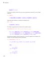
Solve Equations Numerically . . . . . . . . . . . . . . . . . . . . . . . . .
Get Numeric Results . . . . . . . . . . . . . . . . . . . . . . . . . . . . . .
Solve Polynomial Equations and Systems . . . . . . . . . . . . . .
Solve Arbitrary Algebraic Equations and Systems . . . . . . . .
Isolate Numeric Roots . . . . . . . . . . . . . . . . . . . . . . . . . . . . .
Solve Differential Equations and Systems . . . . . . . . . . . . . .
3-73
3-73
3-75
3-76
3-82
3-82
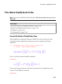
Use General Simplification Functions . . . . . . . . . . . . . . . . .
When to Use General Simplifiers . . . . . . . . . . . . . . . . . . . .
Choose simplify or Simplify . . . . . . . . . . . . . . . . . . . . . . . . .
Use Options to Control Simplification Algorithms . . . . . . . .
3-89
3-89
3-90
3-90
Choose Simplification Functions . . . . . . . . . . . . . . . . . . . . . .
Collect Terms with Same Powers . . . . . . . . . . . . . . . . . . . .
Combine Terms of Same Algebraic Structures . . . . . . . . . . .
Expand Expressions . . . . . . . . . . . . . . . . . . . . . . . . . . . . . .
Factor Expressions . . . . . . . . . . . . . . . . . . . . . . . . . . . . . . .
Compute Normal Forms of Expressions . . . . . . . . . . . . . . . .
Compute Partial Fraction Decompositions of Expressions . .
Simplify Radicals in Arithmetic Expressions . . . . . . . . . . . .
Extract Real and Imaginary Parts of Complex Expressions
Rewrite Expressions in Terms of Other Functions . . . . . . .
3-93
3-94
3-95
3-96
3-97
3-98
3-99
3-99
3-100
3-100
If You Want to Simplify Results Further . . . . . . . . . . . . . .
Increase the Number of Simplification Steps . . . . . . . . . . .
Apply Several Simplification Functions . . . . . . . . . . . . . . .
Use Options . . . . . . . . . . . . . . . . . . . . . . . . . . . . . . . . . . . .
Use Assumptions . . . . . . . . . . . . . . . . . . . . . . . . . . . . . . . .
3-103
3-103
3-104
3-105
3-106
3-68
3-71
Convert Expressions Involving Special Functions . . . . . .
Simplify Special Functions Automatically . . . . . . . . . . . . .
Use General Simplifiers to Reduce Special Functions . . . .
Expand Expressions Involving Special Functions . . . . . . .
Verify Solutions Involving Special Functions . . . . . . . . . . .
3-108
3-108
3-109
3-110
3-110
When to Use Assumptions . . . . . . . . . . . . . . . . . . . . . . . . . . .
3-114
Use Permanent Assumptions . . . . . . . . . . . . . . . . . . . . . . . .
Set Permanent Assumptions . . . . . . . . . . . . . . . . . . . . . . .
Add Permanent Assumptions . . . . . . . . . . . . . . . . . . . . . .
Clear Permanent Assumptions . . . . . . . . . . . . . . . . . . . . .
3-116
3-116
3-118
3-120
Use Temporary Assumptions . . . . . . . . . . . . . . . . . . . . . . . .
Create Temporary Assumptions . . . . . . . . . . . . . . . . . . . .
Assign Temporary Values to Parameters . . . . . . . . . . . . . .
Interactions Between Temporary and Permanent
Assumptions . . . . . . . . . . . . . . . . . . . . . . . . . . . . . . . . .
Use Temporary Assumptions on Top of Permanent
Assumptions . . . . . . . . . . . . . . . . . . . . . . . . . . . . . . . . .
3-122
3-122
3-124
Choose Differentiation Function . . . . . . . . . . . . . . . . . . . . .
3-127
Differentiate Expressions . . . . . . . . . . . . . . . . . . . . . . . . . . .
3-128
Differentiate Functions . . . . . . . . . . . . . . . . . . . . . . . . . . . . .
3-130
Compute Indefinite Integrals . . . . . . . . . . . . . . . . . . . . . . . .
3-135
Compute Definite Integrals . . . . . . . . . . . . . . . . . . . . . . . . .
3-138
Compute Multiple Integrals . . . . . . . . . . . . . . . . . . . . . . . . .
3-141
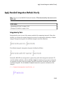
Apply Standard Integration Methods Directly . . . . . . . . . .
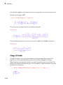
Integration by Parts . . . . . . . . . . . . . . . . . . . . . . . . . . . . .
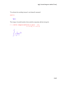
Change of Variable . . . . . . . . . . . . . . . . . . . . . . . . . . . . . .
3-143
3-143
3-144
Get Simpler Results . . . . . . . . . . . . . . . . . . . . . . . . . . . . . . . .
3-146
If an Integral Is Undefined . . . . . . . . . . . . . . . . . . . . . . . . . .
3-147
If MuPAD Cannot Compute an Integral . . . . . . . . . . . . . . .
Approximate Indefinite Integrals . . . . . . . . . . . . . . . . . . .
3-148
3-148
3-125
3-126
ix
x
Contents
Approximate Definite Integrals . . . . . . . . . . . . . . . . . . . . .
3-149
Compute Symbolic Sums . . . . . . . . . . . . . . . . . . . . . . . . . . . .
Indefinite Sums . . . . . . . . . . . . . . . . . . . . . . . . . . . . . . . . .
Definite Sums . . . . . . . . . . . . . . . . . . . . . . . . . . . . . . . . . .
Sums Over Roots of a Polynomial . . . . . . . . . . . . . . . . . . .
3-151
3-151
3-152
3-153
Approximate Sums Numerically . . . . . . . . . . . . . . . . . . . . .
3-154
Compute Taylor Series for Univariate Expressions . . . . .
3-156
Compute Taylor Series for Multivariate Expressions . . . .
3-159
Control Number of Terms in Series Expansions . . . . . . . .
3-160
O-term (The Landau Symbol) . . . . . . . . . . . . . . . . . . . . . . . .
3-163
Compute Generalized Series . . . . . . . . . . . . . . . . . . . . . . . .
3-164
Compute Bidirectional Limits . . . . . . . . . . . . . . . . . . . . . . .
3-166
Compute Right and Left Limits . . . . . . . . . . . . . . . . . . . . . .
3-167
If Limits Do Not Exist . . . . . . . . . . . . . . . . . . . . . . . . . . . . . .
3-170
Create Matrices . . . . . . . . . . . . . . . . . . . . . . . . . . . . . . . . . . .
3-172
Create Vectors . . . . . . . . . . . . . . . . . . . . . . . . . . . . . . . . . . . .
3-174
Create Special Matrices . . . . . . . . . . . . . . . . . . . . . . . . . . . .
3-175
Access and Modify Matrix Elements . . . . . . . . . . . . . . . . . .
Use Loops to Modify Matrix Elements . . . . . . . . . . . . . . . .
Use Functions to Modify Matrix Elements . . . . . . . . . . . .
3-177
3-177
3-178
Create Matrices over Particular Rings . . . . . . . . . . . . . . . .
3-179
Use Sparse and Dense Matrices . . . . . . . . . . . . . . . . . . . . . .
3-181
Compute with Matrices . . . . . . . . . . . . . . . . . . . . . . . . . . . . .
Basic Arithmetic Operations . . . . . . . . . . . . . . . . . . . . . . .
More Operations Available for Matrices . . . . . . . . . . . . . .
3-183
3-183
3-184
Compute Determinants and Traces of Square Matrices . .
3-188
Invert Matrices . . . . . . . . . . . . . . . . . . . . . . . . . . . . . . . . . . . .
3-189
Transpose Matrices . . . . . . . . . . . . . . . . . . . . . . . . . . . . . . . .
3-190
Swap and Delete Rows and Columns . . . . . . . . . . . . . . . . .
3-191
Compute Dimensions of a Matrix . . . . . . . . . . . . . . . . . . . .
3-193
Compute Reduced Row Echelon Form . . . . . . . . . . . . . . . .
3-194
Compute Rank of a Matrix . . . . . . . . . . . . . . . . . . . . . . . . . .
3-195
Compute Bases for Null Spaces of Matrices . . . . . . . . . . . .
3-196
Find Eigenvalues and Eigenvectors . . . . . . . . . . . . . . . . . .
3-197
Find Jordan Canonical Form of a Matrix . . . . . . . . . . . . . .
3-200
Compute Matrix Exponentials . . . . . . . . . . . . . . . . . . . . . . .
3-202
Compute Cholesky Factorization . . . . . . . . . . . . . . . . . . . . .
3-203
Compute LU Factorization . . . . . . . . . . . . . . . . . . . . . . . . . .
3-206
Compute QR Factorization . . . . . . . . . . . . . . . . . . . . . . . . . .
3-208
Compute Determinant Numerically . . . . . . . . . . . . . . . . . .
3-210
Compute Eigenvalues and Eigenvectors Numerically . . . .
3-214
Compute Factorizations Numerically . . . . . . . . . . . . . . . . .
Cholesky Decomposition . . . . . . . . . . . . . . . . . . . . . . . . . .
LU Decomposition . . . . . . . . . . . . . . . . . . . . . . . . . . . . . . .
QR Decomposition . . . . . . . . . . . . . . . . . . . . . . . . . . . . . . .
Singular Value Decomposition . . . . . . . . . . . . . . . . . . . . . .
3-219
3-219
3-220
3-222
3-224
Mathematical Constants Available in MuPAD . . . . . . . . . .
Special Real Numbers . . . . . . . . . . . . . . . . . . . . . . . . . . . .
Infinities . . . . . . . . . . . . . . . . . . . . . . . . . . . . . . . . . . . . . .
Boolean Constants . . . . . . . . . . . . . . . . . . . . . . . . . . . . . . .
3-227
3-227
3-228
3-228
xi
xii
Contents
Special Values . . . . . . . . . . . . . . . . . . . . . . . . . . . . . . . . . .
Special Sets . . . . . . . . . . . . . . . . . . . . . . . . . . . . . . . . . . . .
3-228
3-229
Special Functions Available in MuPAD . . . . . . . . . . . . . . .
Dirac and Heaviside Functions . . . . . . . . . . . . . . . . . . . . .
Gamma Functions . . . . . . . . . . . . . . . . . . . . . . . . . . . . . . .
Zeta Function and Polylogarithms . . . . . . . . . . . . . . . . . . .
Airy and Bessel Functions . . . . . . . . . . . . . . . . . . . . . . . . .
Exponential and Trigonometric Integrals . . . . . . . . . . . . .
Error Functions and Fresnel Functions . . . . . . . . . . . . . . .
Hypergeometric, Meijer G, and Whittaker Functions . . . . .
Elliptic Integrals . . . . . . . . . . . . . . . . . . . . . . . . . . . . . . . .
Lambert W Function (omega Function) . . . . . . . . . . . . . . .
3-230
3-230
3-230
3-231
3-231
3-231
3-232
3-232
3-233
3-233
Floating-Point Arguments and Function Sensitivity . . . . .
Use Symbolic Computations When Possible . . . . . . . . . . . .
Increase Precision . . . . . . . . . . . . . . . . . . . . . . . . . . . . . . .
Approximate Parameters and Approximate Results . . . . . .
Plot Special Functions . . . . . . . . . . . . . . . . . . . . . . . . . . . .
3-234
3-235
3-235
3-237
3-238
Integral Transforms . . . . . . . . . . . . . . . . . . . . . . . . . . . . . . . .
Fourier and Inverse Fourier Transforms . . . . . . . . . . . . . .
Laplace and Inverse Laplace Transforms . . . . . . . . . . . . .
3-242
3-242
3-245
Z-Transforms . . . . . . . . . . . . . . . . . . . . . . . . . . . . . . . . . . . . . .
3-249
Discrete Fourier Transforms . . . . . . . . . . . . . . . . . . . . . . . .
3-252
Use Custom Patterns for Transforms . . . . . . . . . . . . . . . . .
Add New Patterns . . . . . . . . . . . . . . . . . . . . . . . . . . . . . . .
Overwrite Existing Patterns . . . . . . . . . . . . . . . . . . . . . . .
3-257
3-257
3-259
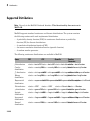
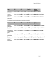
Supported Distributions . . . . . . . . . . . . . . . . . . . . . . . . . . . .
3-260
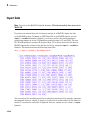
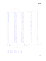
Import Data . . . . . . . . . . . . . . . . . . . . . . . . . . . . . . . . . . . . . .
3-262
Store Statistical Data . . . . . . . . . . . . . . . . . . . . . . . . . . . . . .
3-266
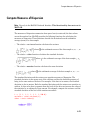
Compute Measures of Central Tendency . . . . . . . . . . . . . .
3-267
Compute Measures of Dispersion . . . . . . . . . . . . . . . . . . . .
3-271
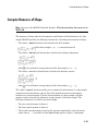
Compute Measures of Shape . . . . . . . . . . . . . . . . . . . . . . . .
3-273
Compute Covariance and Correlation . . . . . . . . . . . . . . . .
3-276
Handle Outliers . . . . . . . . . . . . . . . . . . . . . . . . . . . . . . . . . . .
3-278
Bin Data . . . . . . . . . . . . . . . . . . . . . . . . . . . . . . . . . . . . . . . . .
3-279
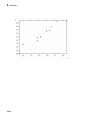
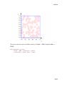
Create Scatter and List Plots . . . . . . . . . . . . . . . . . . . . . . . .
3-281
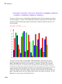
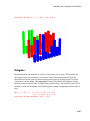
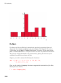
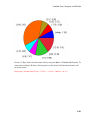
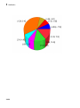
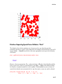
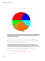
Create Bar Charts, Histograms, and Pie Charts . . . . . . . .
Bar Charts . . . . . . . . . . . . . . . . . . . . . . . . . . . . . . . . . . . .
Histograms . . . . . . . . . . . . . . . . . . . . . . . . . . . . . . . . . . . .
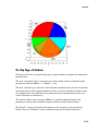
Pie Charts . . . . . . . . . . . . . . . . . . . . . . . . . . . . . . . . . . . . .
3-285
3-285
3-287
3-288
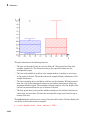
Create Box Plots . . . . . . . . . . . . . . . . . . . . . . . . . . . . . . . . . .
3-293
Create Quantile-Quantile Plots . . . . . . . . . . . . . . . . . . . . . .
3-296
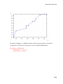
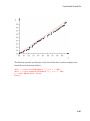
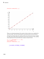
Univariate Linear Regression . . . . . . . . . . . . . . . . . . . . . . .
3-299
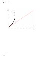
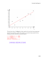
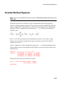
Univariate Nonlinear Regression . . . . . . . . . . . . . . . . . . . .
3-303
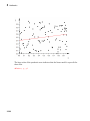
Multivariate Regression . . . . . . . . . . . . . . . . . . . . . . . . . . . .
3-306
Principles of Hypothesis Testing . . . . . . . . . . . . . . . . . . . . .
3-309
Perform chi-square Test . . . . . . . . . . . . . . . . . . . . . . . . . . . .
3-310
Perform Kolmogorov-Smirnov Test . . . . . . . . . . . . . . . . . . .
3-312
Perform Shapiro-Wilk Test . . . . . . . . . . . . . . . . . . . . . . . . . .
3-313
Perform t-Test . . . . . . . . . . . . . . . . . . . . . . . . . . . . . . . . . . . .
3-314
Divisors . . . . . . . . . . . . . . . . . . . . . . . . . . . . . . . . . . . . . . . . . .
Compute Divisors and Number of Divisors . . . . . . . . . . . .
Compute Greatest Common Divisors . . . . . . . . . . . . . . . . .
Compute Least Common Multiples . . . . . . . . . . . . . . . . . .
3-315
3-315
3-316
3-317
Primes and Factorizations . . . . . . . . . . . . . . . . . . . . . . . . . .
Operate on Primes . . . . . . . . . . . . . . . . . . . . . . . . . . . . . .
Factorizations . . . . . . . . . . . . . . . . . . . . . . . . . . . . . . . . . .
Prove Primality . . . . . . . . . . . . . . . . . . . . . . . . . . . . . . . . .
3-318
3-318
3-320
3-320
xiii
4
xiv
Contents
Modular Arithmetic . . . . . . . . . . . . . . . . . . . . . . . . . . . . . . . .
Quotients and Remainders . . . . . . . . . . . . . . . . . . . . . . . .
Common Modular Arithmetic Operations . . . . . . . . . . . . .
Residue Class Rings and Fields . . . . . . . . . . . . . . . . . . . . .
3-322
3-322
3-324
3-325
Congruences . . . . . . . . . . . . . . . . . . . . . . . . . . . . . . . . . . . . . .
Linear Congruences . . . . . . . . . . . . . . . . . . . . . . . . . . . . . .
Systems of Linear Congruences . . . . . . . . . . . . . . . . . . . . .
Modular Square Roots . . . . . . . . . . . . . . . . . . . . . . . . . . . .
General Solver for Congruences . . . . . . . . . . . . . . . . . . . .
3-327
3-327
3-328
3-329
3-332
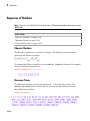
Sequences of Numbers . . . . . . . . . . . . . . . . . . . . . . . . . . . . .
Fibonacci Numbers . . . . . . . . . . . . . . . . . . . . . . . . . . . . . .
Mersenne Primes . . . . . . . . . . . . . . . . . . . . . . . . . . . . . . . .
Continued Fractions . . . . . . . . . . . . . . . . . . . . . . . . . . . . .
3-334
3-334
3-334
3-335
Programming Basics
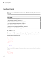
Conditional Control . . . . . . . . . . . . . . . . . . . . . . . . . . . . . . . . . .
Use if Statements . . . . . . . . . . . . . . . . . . . . . . . . . . . . . . . . .
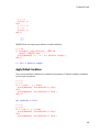
Apply Multiple Conditions . . . . . . . . . . . . . . . . . . . . . . . . . .
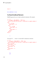
Use Nested Conditional Statements . . . . . . . . . . . . . . . . . . .
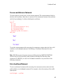
Use case and otherwise Statements . . . . . . . . . . . . . . . . . . .
Exit a Conditional Statement . . . . . . . . . . . . . . . . . . . . . . . .
Return Value of a Conditional Statement . . . . . . . . . . . . . . .
Display Intermediate Results . . . . . . . . . . . . . . . . . . . . . . . .
4-2
4-2
4-3
4-4
4-5
4-5
4-6
4-7
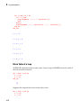
Loops . . . . . . . . . . . . . . . . . . . . . . . . . . . . . . . . . . . . . . . . . . . . . .
Use Loops with a Fixed Number of Iterations (for Loops) . . .
Use Loops with Conditions (while and repeat Loops) . . . . . .
Use Nested Loops . . . . . . . . . . . . . . . . . . . . . . . . . . . . . . . .
Exit a Loop . . . . . . . . . . . . . . . . . . . . . . . . . . . . . . . . . . . . .
Skip Part of Iteration . . . . . . . . . . . . . . . . . . . . . . . . . . . . .
Return Value of a Loop . . . . . . . . . . . . . . . . . . . . . . . . . . . .
Display Intermediate Results . . . . . . . . . . . . . . . . . . . . . . .
4-8
4-8
4-10
4-13
4-14
4-15
4-16
4-17
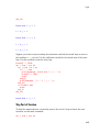
Procedures . . . . . . . . . . . . . . . . . . . . . . . . . . . . . . . . . . . . . . . .
Create a Procedure . . . . . . . . . . . . . . . . . . . . . . . . . . . . . . .
Call a Procedure . . . . . . . . . . . . . . . . . . . . . . . . . . . . . . . . .
4-18
4-18
4-18
Control Return Values . . . . . . . . . . . . . . . . . . . . . . . . . . . .
Return Multiple Results . . . . . . . . . . . . . . . . . . . . . . . . . . .
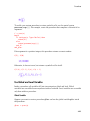
Return Symbolic Calls . . . . . . . . . . . . . . . . . . . . . . . . . . . . .
Use Global and Local Variables . . . . . . . . . . . . . . . . . . . . .
Restore Values and Properties of Global Variables Modified in
Procedures . . . . . . . . . . . . . . . . . . . . . . . . . . . . . . . . . . . .
5
4-19
4-20
4-20
4-21
4-23
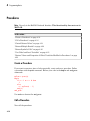
Functions . . . . . . . . . . . . . . . . . . . . . . . . . . . . . . . . . . . . . . . . .
Call Existing Functions . . . . . . . . . . . . . . . . . . . . . . . . . . . .
Create Functions . . . . . . . . . . . . . . . . . . . . . . . . . . . . . . . . .
Evaluate Expressions While Creating Functions . . . . . . . . .
Use Functions with Parameters . . . . . . . . . . . . . . . . . . . . .
4-26
4-26
4-26
4-27
4-28
Shortcut for Closing Statements . . . . . . . . . . . . . . . . . . . . . .
4-29
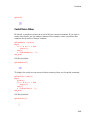
Programming Fundamentals
Data Type Definition . . . . . . . . . . . . . . . . . . . . . . . . . . . . . . . . .
Domain Types . . . . . . . . . . . . . . . . . . . . . . . . . . . . . . . . . . . .
Expression Types . . . . . . . . . . . . . . . . . . . . . . . . . . . . . . . . .
5-3
5-3
5-3
Sequences . . . . . . . . . . . . . . . . . . . . . . . . . . . . . . . . . . . . . . . . . .
Create Sequences . . . . . . . . . . . . . . . . . . . . . . . . . . . . . . . . .
Access Sequence Entries . . . . . . . . . . . . . . . . . . . . . . . . . . . .
Add, Replace, or Remove Sequence Entries . . . . . . . . . . . . . .
5-6
5-6
5-7
5-8
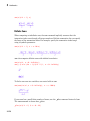
Lists . . . . . . . . . . . . . . . . . . . . . . . . . . . . . . . . . . . . . . . . . . . . . .
Create Lists . . . . . . . . . . . . . . . . . . . . . . . . . . . . . . . . . . . . .
Access List Entries . . . . . . . . . . . . . . . . . . . . . . . . . . . . . . .
Operate on Lists . . . . . . . . . . . . . . . . . . . . . . . . . . . . . . . . .
Add, Replace, or Remove List Entries . . . . . . . . . . . . . . . . .
5-10
5-10
5-11
5-12
5-16
Sets . . . . . . . . . . . . . . . . . . . . . . . . . . . . . . . . . . . . . . . . . . . . . . .
Create Sets . . . . . . . . . . . . . . . . . . . . . . . . . . . . . . . . . . . . .
Access Set Elements . . . . . . . . . . . . . . . . . . . . . . . . . . . . . .
Operate on Sets . . . . . . . . . . . . . . . . . . . . . . . . . . . . . . . . . .
Add, Replace, or Remove Set Elements . . . . . . . . . . . . . . . .
5-18
5-18
5-19
5-20
5-22
xv
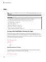
Tables . . . . . . . . . . . . . . . . . . . . . . . . . . . . . . . . . . . . . . . . . . . . .
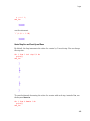
Create Tables . . . . . . . . . . . . . . . . . . . . . . . . . . . . . . . . . . .
Access Table Elements . . . . . . . . . . . . . . . . . . . . . . . . . . . .
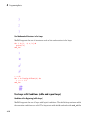
Operate on Tables . . . . . . . . . . . . . . . . . . . . . . . . . . . . . . . .
Replace or Remove Table Entries . . . . . . . . . . . . . . . . . . . .
5-25
5-25
5-26
5-27
5-28
Arrays . . . . . . . . . . . . . . . . . . . . . . . . . . . . . . . . . . . . . . . . . . . .
Create Arrays . . . . . . . . . . . . . . . . . . . . . . . . . . . . . . . . . . .
Access Array Entries . . . . . . . . . . . . . . . . . . . . . . . . . . . . . .
Operate on Arrays . . . . . . . . . . . . . . . . . . . . . . . . . . . . . . . .
Replace or Remove Array Entries . . . . . . . . . . . . . . . . . . . .
Arrays with Hardware Floating-Point Numbers . . . . . . . . .
5-30
5-30
5-31
5-32
5-34
5-34
Vectors and Matrices . . . . . . . . . . . . . . . . . . . . . . . . . . . . . . . .
Create Matrices . . . . . . . . . . . . . . . . . . . . . . . . . . . . . . . . . .
Create Vectors . . . . . . . . . . . . . . . . . . . . . . . . . . . . . . . . . . .
Combine Vectors into a Matrix . . . . . . . . . . . . . . . . . . . . . .
Matrices Versus Arrays . . . . . . . . . . . . . . . . . . . . . . . . . . . .
Convert Matrices and Arrays . . . . . . . . . . . . . . . . . . . . . . .
5-36
5-36
5-37
5-37
5-38
5-38
Choose Appropriate Data Structures . . . . . . . . . . . . . . . . . .
5-40
Data Types . . . . . . . . . . . . . . . . . . . . . . . . . . . . . . . . .
the coerce Function . . . . . . . . . . . . . . . . . . . . . . . . . . .
the expr Function . . . . . . . . . . . . . . . . . . . . . . . . . . . . .
Constructors . . . . . . . . . . . . . . . . . . . . . . . . . . . . . . . . .
5-42
5-43
5-44
5-47
Define Your Own Data Types . . . . . . . . . . . . . . . . . . . . . . . . .
5-49
Access Arguments of a Procedure . . . . . . . . . . . . . . . . . . . . .
5-52
Test Arguments . . . . . . . . . . . . . . . . . . . . . . . . . . . . . . . . . . . .
Check Types of Arguments . . . . . . . . . . . . . . . . . . . . . . . . .
Check Arguments of Individual Procedures . . . . . . . . . . . . .
5-55
5-55
5-57
Verify Options . . . . . . . . . . . . . . . . . . . . . . . . . . . . . . . . . . . . .
5-60
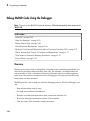
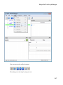
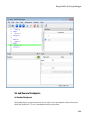
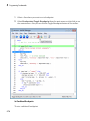
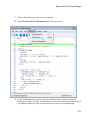
Debug MuPAD Code Using the Debugger . . . . . . . . . . . . . . .
Overview . . . . . . . . . . . . . . . . . . . . . . . . . . . . . . . . . . . . . . .
Open the Debugger . . . . . . . . . . . . . . . . . . . . . . . . . . . . . . .
Debug Step-by-Step . . . . . . . . . . . . . . . . . . . . . . . . . . . . . . .
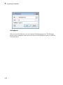
Set and Remove Breakpoints . . . . . . . . . . . . . . . . . . . . . . .
5-64
5-64
5-65
5-66
5-69
Convert
Use
Use
Use
xvi
Contents
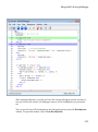
Evaluate Variables and Expressions After a Particular
Function Call . . . . . . . . . . . . . . . . . . . . . . . . . . . . . . . . .
Watch Intermediate Values of Variables and Expressions . .
View Names of Currently Running Procedures . . . . . . . . . .
Correct Errors . . . . . . . . . . . . . . . . . . . . . . . . . . . . . . . . . . .
5-75
5-77
5-78
5-79
Debug MuPAD Code in the Tracing Mode . . . . . . . . . . . . . .
5-81
Display Progress . . . . . . . . . . . . . . . . . . . . . . . . . . . . . . . . . . .
5-85
Use Assertions . . . . . . . . . . . . . . . . . . . . . . . . . . . . . . . . . . . . .
5-88
Write Error and Warning Messages . . . . . . . . . . . . . . . . . . .
5-90
Handle Errors . . . . . . . . . . . . . . . . . . . . . . . . . . . . . . . . . . . . . .
5-92
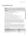
When to Analyze Performance . . . . . . . . . . . . . . . . . . . . . . . .
5-95
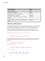
Measure Time . . . . . . . . . . . . . . . . . . . . . . . . . . . . . . . . . . . . . .
Calls to MuPAD Processes . . . . . . . . . . . . . . . . . . . . . . . . .
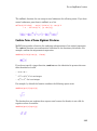
Calls to External Processes . . . . . . . . . . . . . . . . . . . . . . . . .
5-96
5-96
5-99
Profile Your Code . . . . . . . . . . . . . . . . . . . . . . . . . . . . . . . . .
5-100
Techniques for Improving Performance . . . . . . . . . . . . . . .
5-109
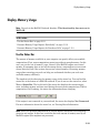
Display Memory Usage . . . . . . . . . . . . . . . . . . . . . . . . . . . . .
Use the Status Bar . . . . . . . . . . . . . . . . . . . . . . . . . . . . . .
Generate Memory Usage Reports Periodically . . . . . . . . . .
Generate Memory Usage Reports for Procedure Calls . . . .
5-111
5-111
5-112
5-113
Remember Mechanism . . . . . . . . . . . . . . . . . . . . . . . . . . . . .
Why Use the Remember Mechanism . . . . . . . . . . . . . . . . .
Remember Results Without Context . . . . . . . . . . . . . . . . .
Remember Results and Context . . . . . . . . . . . . . . . . . . . .
Clear Remember Tables . . . . . . . . . . . . . . . . . . . . . . . . . .
Potential Problems Related to the Remember Mechanism .
5-115
5-115
5-117
5-118
5-119
5-121
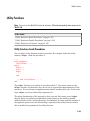
History Mechanism . . . . . . . . . . . . . . . . . . . . . . . . . . . . . . . .
Access the History Table . . . . . . . . . . . . . . . . . . . . . . . . . .
Specify Maximum Number of Entries . . . . . . . . . . . . . . . .
Clear the History Table . . . . . . . . . . . . . . . . . . . . . . . . . . .
5-123
5-123
5-126
5-127
xvii
xviii
Contents
Why Test Your Code . . . . . . . . . . . . . . . . . . . . . . . . . . . . . . .
5-128
Write Single Tests . . . . . . . . . . . . . . . . . . . . . . . . . . . . . . . . .
5-130
Write Test Scripts . . . . . . . . . . . . . . . . . . . . . . . . . . . . . . . . .
5-134
Code Verification . . . . . . . . . . . . . . . . . . . . . . . . . . . . . . . . . .
5-138
Protect Function and Option Names . . . . . . . . . . . . . . . . . .
5-140
Data Collection . . . . . . . . . . . . . . . . . . . . . . . . . . . . . . . . . . . .
Parallel Collection . . . . . . . . . . . . . . . . . . . . . . . . . . . . . . .
Fixed-Length Collection . . . . . . . . . . . . . . . . . . . . . . . . . . .
Known-Maximum-Length Collection . . . . . . . . . . . . . . . . .
Unknown-Maximum-Length Collection . . . . . . . . . . . . . . .
5-142
5-142
5-144
5-145
5-146
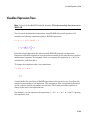
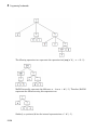
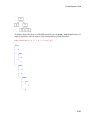
Visualize Expression Trees . . . . . . . . . . . . . . . . . . . . . . . . . .
5-149
Modify Subexpressions . . . . . . . . . . . . . . . . . . . . . . . . . . . . .
Find and Replace Subexpressions . . . . . . . . . . . . . . . . . . .
Recursive Substitution . . . . . . . . . . . . . . . . . . . . . . . . . . .
5-152
5-152
5-155
Variables Inside Procedures . . . . . . . . . . . . . . . . . . . . . . . .
Closures . . . . . . . . . . . . . . . . . . . . . . . . . . . . . . . . . . . . . . .
Static Variables . . . . . . . . . . . . . . . . . . . . . . . . . . . . . . . . .
5-158
5-158
5-160
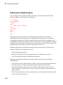
Utility Functions . . . . . . . . . . . . . . . . . . . . . . . . . . . . . . . . . .
Utility Functions Inside Procedures . . . . . . . . . . . . . . . . .
Utility Functions Outside Procedures . . . . . . . . . . . . . . . .
Utility Functions in Closures . . . . . . . . . . . . . . . . . . . . . .
5-163
5-163
5-164
5-165
Private Methods . . . . . . . . . . . . . . . . . . . . . . . . . . . . . . . . . . .
5-167
Calls by Reference and Calls by Value . . . . . . . . . . . . . . . .
Calls by Value . . . . . . . . . . . . . . . . . . . . . . . . . . . . . . . . . .
Calls by Reference . . . . . . . . . . . . . . . . . . . . . . . . . . . . . . .
5-169
5-169
5-170
Integrate Custom Functions into MuPAD . . . . . . . . . . . . .
5-176
6
Graphics and Animations
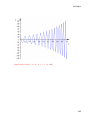
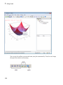
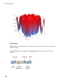
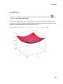
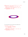
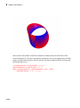
Gallery . . . . . . . . . . . . . . . . . . . . . . . . . . . . . . . . . . . . . . . . . . . . .
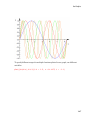
2D Function and Curve Plots . . . . . . . . . . . . . . . . . . . . . . . .
Other 2D examples . . . . . . . . . . . . . . . . . . . . . . . . . . . . . . . .
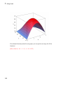
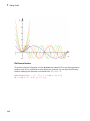
3D Functions, Surfaces, and Curves . . . . . . . . . . . . . . . . . .
6-2
6-2
6-7
6-17
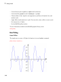
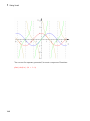
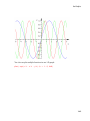
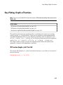
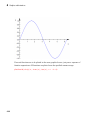
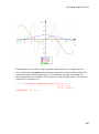
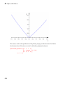
Easy Plotting: Graphs of Functions . . . . . . . . . . . . . . . . . . .
2D Function Graphs: plotfunc2d . . . . . . . . . . . . . . . . . . .
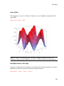
3D Function Graphs: plotfunc3d . . . . . . . . . . . . . . . . . . .
Attributes for plotfunc2d and plotfunc3d . . . . . . . . . . .
6-25
6-25
6-41
6-56
Advanced Plotting: Principles and First Examples . . . . . . .
General Principles . . . . . . . . . . . . . . . . . . . . . . . . . . . . . . . .
Some Examples . . . . . . . . . . . . . . . . . . . . . . . . . . . . . . . . . .
6-78
6-78
6-84
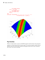
The Full Picture: Graphical Trees . . . . . . . . . . . . . . . . . . . . .
6-93
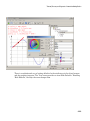
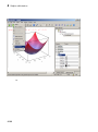
Viewer, Browser, and Inspector: Interactive Manipulation
6-98
Primitives . . . . . . . . . . . . . . . . . . . . . . . . . . . . . . . . . . . . . . . .
6-103
Attributes . . . . . . . . . . . . . . . . . . . . . . . . . . . . . . . . . . . . . . . .
Default Values . . . . . . . . . . . . . . . . . . . . . . . . . . . . . . . . . .
Inheritance of Attributes . . . . . . . . . . . . . . . . . . . . . . . . . .
Primitives Requesting Special Scene Attributes: “Hints” . .
The Help Pages of Attributes . . . . . . . . . . . . . . . . . . . . . .
6-108
6-109
6-110
6-117
6-119
Layout of Canvas and Scenes . . . . . . . . . . . . . . . . . . . . . . . .
Layout of the Canvas . . . . . . . . . . . . . . . . . . . . . . . . . . . .
Layout of Scenes . . . . . . . . . . . . . . . . . . . . . . . . . . . . . . . .
6-120
6-120
6-126
Animations . . . . . . . . . . . . . . . . . . . . . . . . . . . . . . . . . . . . . . .
Generate Simple Animations . . . . . . . . . . . . . . . . . . . . . . .
Play Animations . . . . . . . . . . . . . . . . . . . . . . . . . . . . . . . .
The Number of Frames and the Time Range . . . . . . . . . . .
What Can Be Animated? . . . . . . . . . . . . . . . . . . . . . . . . . .
Advanced Animations: The Synchronization Model . . . . . .
Frame by Frame Animations . . . . . . . . . . . . . . . . . . . . . . .
Examples . . . . . . . . . . . . . . . . . . . . . . . . . . . . . . . . . . . . . .
6-129
6-129
6-134
6-135
6-138
6-140
6-143
6-149
xix
7
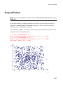
Groups of Primitives . . . . . . . . . . . . . . . . . . . . . . . . . . . . . . .
6-157
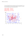
Transformations . . . . . . . . . . . . . . . . . . . . . . . . . . . . . . . . . . .
6-159
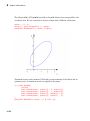
Legends . . . . . . . . . . . . . . . . . . . . . . . . . . . . . . . . . . . . . . . . . .
6-164
Fonts . . . . . . . . . . . . . . . . . . . . . . . . . . . . . . . . . . . . . . . . . . . .
6-168
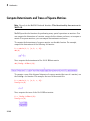
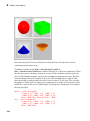
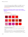
Colors . . . . . . . . . . . . . . . . . . . . . . . . . . . . . . . . . . . . . . . . . . . .
RGB Colors . . . . . . . . . . . . . . . . . . . . . . . . . . . . . . . . . . . .
HSV Colors . . . . . . . . . . . . . . . . . . . . . . . . . . . . . . . . . . . .
6-171
6-171
6-174
Save and Export Pictures . . . . . . . . . . . . . . . . . . . . . . . . . . .
Save and Export Interactively . . . . . . . . . . . . . . . . . . . . . .
Save in Batch Mode . . . . . . . . . . . . . . . . . . . . . . . . . . . . .
6-176
6-176
6-176
Import Pictures . . . . . . . . . . . . . . . . . . . . . . . . . . . . . . . . . . .
6-179
Cameras in 3D . . . . . . . . . . . . . . . . . . . . . . . . . . . . . . . . . . . .
6-181
Possible Strange Effects in 3D . . . . . . . . . . . . . . . . . . . . . . .
6-192
Quick Reference
Glossary . . . . . . . . . . . . . . . . . . . . . . . . . . . . . . . . . . . . . . . . . . . .
8
xx
Contents
7-2
More Information About Some of the MuPAD
Libraries
Abstract Data Types Library . . . . . . . . . . . . . . . . . . . . . . . . . .
Example . . . . . . . . . . . . . . . . . . . . . . . . . . . . . . . . . . . . . . . .
8-2
8-2
Axioms . . . . . . . . . . . . . . . . . . . . . . . . . . . . . . . . . . . . . . . . . . . . .
Bibliography . . . . . . . . . . . . . . . . . . . . . . . . . . . . . . . . . . . . .
8-4
8-4
Categories . . . . . . . . . . . . . . . . . . . . . . . . . . . . . . . . . . . . . . . . . .
Introduction . . . . . . . . . . . . . . . . . . . . . . . . . . . . . . . . . . . . .
Category Constructors . . . . . . . . . . . . . . . . . . . . . . . . . . . . . .
Bibliography . . . . . . . . . . . . . . . . . . . . . . . . . . . . . . . . . . . . .
8-5
8-5
8-6
8-6
Combinatorics . . . . . . . . . . . . . . . . . . . . . . . . . . . . . . . . . . . . . .
8-7
Functional Programming . . . . . . . . . . . . . . . . . . . . . . . . . . . . .
8-8
Gröbner bases . . . . . . . . . . . . . . . . . . . . . . . . . . . . . . . . . . . . .
8-10
The import Library . . . . . . . . . . . . . . . . . . . . . . . . . . . . . . . . .
8-11
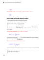
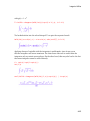
Integration Utilities . . . . . . . . . . . . . . . . . . . . . . . . . . . . . . . . .
First steps . . . . . . . . . . . . . . . . . . . . . . . . . . . . . . . . . . . . . .
Integration by parts and by change of variables . . . . . . . . .
8-12
8-12
8-14
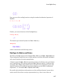
Linear Algebra Library . . . . . . . . . . . . . . . . . . . . . . . . . . . . . .
Introduction . . . . . . . . . . . . . . . . . . . . . . . . . . . . . . . . . . . . .
Data Types for Matrices and Vectors . . . . . . . . . . . . . . . . .
8-16
8-16
8-17
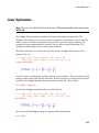
Linear Optimization . . . . . . . . . . . . . . . . . . . . . . . . . . . . . . . .
8-23
The misc Library . . . . . . . . . . . . . . . . . . . . . . . . . . . . . . . . . . .
8-25
Numeric Algorithms Library . . . . . . . . . . . . . . . . . . . . . . . . .
8-26
Orthogonal Polynomials . . . . . . . . . . . . . . . . . . . . . . . . . . . . .
8-27
Properties . . . . . . . . . . . . . . . . . . . . . . . . . . . . . . . . . . . . . . . . .
8-28
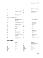
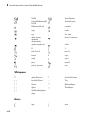
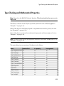
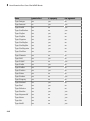
Typeset Symbols in MuPAD . . . . . . . . . . . . . . . . . . . . . . . . . .
Greek Letters . . . . . . . . . . . . . . . . . . . . . . . . . . . . . . . . . . .
Open Face Letters . . . . . . . . . . . . . . . . . . . . . . . . . . . . . . . .
Arrows . . . . . . . . . . . . . . . . . . . . . . . . . . . . . . . . . . . . . . . . .
Operators . . . . . . . . . . . . . . . . . . . . . . . . . . . . . . . . . . . . . .
Comparison Operators . . . . . . . . . . . . . . . . . . . . . . . . . . . . .
Other Symbols . . . . . . . . . . . . . . . . . . . . . . . . . . . . . . . . . . .
Whitespaces . . . . . . . . . . . . . . . . . . . . . . . . . . . . . . . . . . . . .
Braces . . . . . . . . . . . . . . . . . . . . . . . . . . . . . . . . . . . . . . . . .
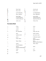
Punctuation Marks . . . . . . . . . . . . . . . . . . . . . . . . . . . . . . .
Umlauts . . . . . . . . . . . . . . . . . . . . . . . . . . . . . . . . . . . . . . .
Currency . . . . . . . . . . . . . . . . . . . . . . . . . . . . . . . . . . . . . . .
8-31
8-31
8-33
8-33
8-34
8-35
8-35
8-36
8-36
8-37
8-38
8-38
xxi
xxii
Contents
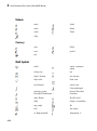
Math Symbols . . . . . . . . . . . . . . . . . . . . . . . . . . . . . . . . . . .
8-38
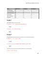
Type Checking and Mathematical Properties . . . . . . . . . . .
Example 1 . . . . . . . . . . . . . . . . . . . . . . . . . . . . . . . . . . . . . .
Example 2 . . . . . . . . . . . . . . . . . . . . . . . . . . . . . . . . . . . . . .
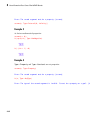
Example 3 . . . . . . . . . . . . . . . . . . . . . . . . . . . . . . . . . . . . . .
Example 4 . . . . . . . . . . . . . . . . . . . . . . . . . . . . . . . . . . . . . .
8-39
8-41
8-41
8-42
8-42
1
Getting Started
• “Desktop Overview” on page 1-2
• “Evaluate Mathematical Expressions and Commands” on page 1-4
• “Shortcut to Access Standard MuPAD Functions” on page 1-7
• “Access Help for Particular Command” on page 1-15
• “Perform Computations” on page 1-19
• “Use Graphics” on page 1-39
• “Use the MuPAD Libraries” on page 1-62
1
Getting Started
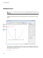
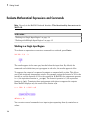
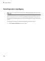
Desktop Overview
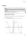
Note: Use only in the MuPAD Notebook Interface. This functionality does not run in
MATLAB.
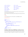
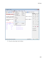
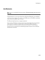
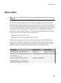
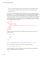
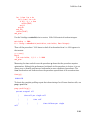
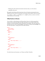
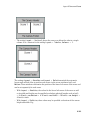
A MuPAD® notebook has three types of regions: input regions, output regions, and text
regions.
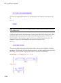
In the input regions, marked by grey brackets, you can type mathematical expressions
and commands in the MuPAD language. For example, type the following expression and
press Enter to evaluate the result:
3*2^10 + 1/3 - 3
1-2
Desktop Overview
The results (including graphics) appear in a new output region. The default font color for
input regions is red, and the default font color for output regions is blue. To customize
default settings, see Changing Default Format Settings.
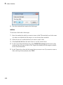
When you evaluate an expression in the bottom input region, MuPAD inserts a new
input region below. To insert new input regions in other parts of a notebook:
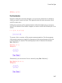
1
Select the place in a notebook where you want to insert a new input region
2
Insert a new input region:
• To insert an input region below the cursor position, select Insert>Calculation
from the main menu.
• To insert an input region above the cursor position, select Insert>Calculation
Above from the main menu.
You can type and format text in a notebook similar to working in any word processing
application. To start a new text region, click outside the gray brackets and start typing.
Also, to insert a new text region, you can select Insert>Text Paragraph or
Insert>Text Paragraph Above. You cannot insert a text region between adjacent input
and output regions.
You can exchange data between different regions in a notebook. For example, you can:
• Copy expressions and commands from the text regions to the input regions and
evaluate them.
• Copy expressions and commands from the input regions to the text regions.
• Copy results including mathematical expressions and graphics from the output
regions to the text regions.
• Copy results from the output regions to the input regions. Mathematical expressions
copied from the output regions appear as valid MuPAD input commands.
You cannot paste data into the output regions. To change the results, edit the associated
input region and evaluate it by pressing Enter.
1-3
1
Getting Started
Evaluate Mathematical Expressions and Commands
Note: Use only in the MuPAD Notebook Interface. This functionality does not run in
MATLAB.
In this section...
“Working in a Single Input Region” on page 1-4
“Working with Multiple Input Regions” on page 1-5
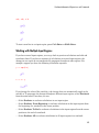
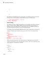
Working in a Single Input Region
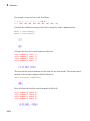
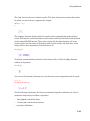
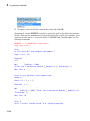
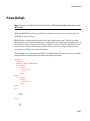
To evaluate an expression or execute a command in a notebook, press Enter:
3*2^10 + 1/3 - 3
The results appear in the same grey bracket below the input data. By default, the
commands and calculations you type appear in red color, the results appear in blue.
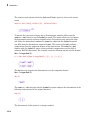
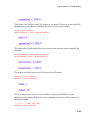
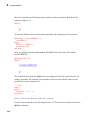
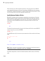
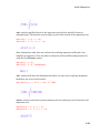
To suppress the output of a command, terminate a command with a colon. This allows
you to hide irrelevant intermediate results. For example, assign the factorial of 123 to the
variable a, and the factorial of 132 to the variable b. In MuPAD, the assignment operator
is := (the equivalent function is _assign). The factorial operator is ! (the equivalent
function is fact). Terminate these assignments with colons to suppress the outputs.
Here MuPAD displays only the result of the division a/b:
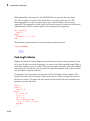
a := 123!: b := 132!: a/b
delete a, b:
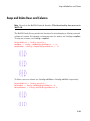
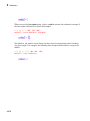
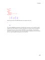
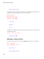
You can enter several commands in an input region separating them by semicolons or
colons:
1-4
Evaluate Mathematical Expressions and Commands
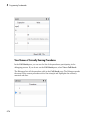
a+b; a*b; a^b
To start a new line in an input region, press Ctrl+Enter or Shift+Enter.
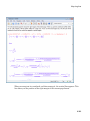
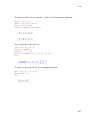
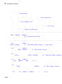
Working with Multiple Input Regions
If you have several input regions, you can go back to previous calculations and edit and
reevaluate them. If you have a sequence of calculations in several input regions, the
changes in one region do not automatically propagate throughout other regions. For
example, suppose you have the following calculation sequence:
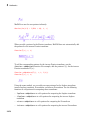
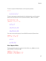
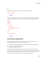
y := exp(2*x)
z := x + y
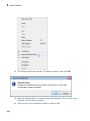
If you change the value of the variable y, the change does not automatically apply to the
variable z. To propagate the change throughout different input regions, select Notebook
from the main menu. From here you can:
• Select Evaluate to evaluate calculations in one input region.
• Select Evaluate From Beginning to evaluate calculations in the input regions from
the beginning of a notebook to the cursor position.
• Select Evaluate To End to evaluate calculations in the input regions from the cursor
position to the end of a notebook.
• Select Evaluate All to evaluate calculations in all input regions in a notebook.
1-5
1
Getting Started
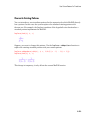
Also, you can propagate the change throughout multiple input regions by pressing Enter
in each input region.
1-6
Shortcut to Access Standard MuPAD Functions
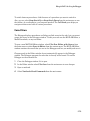
Shortcut to Access Standard MuPAD Functions
Note: Use only in the MuPAD Notebook Interface. This functionality does not run in
MATLAB.
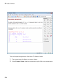
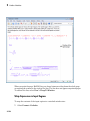
To eliminate syntax errors and to make it easy to remember the commands and
functions, MuPAD can automatically complete the command you start typing. To
automatically complete the command, press Ctrl+space.
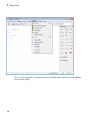
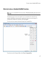
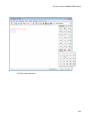
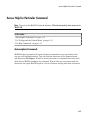
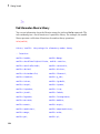
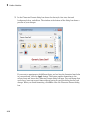
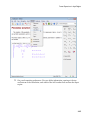
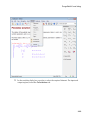
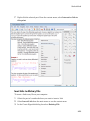
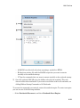
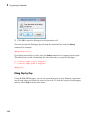
You also can access common functions through the Command Bar.
If you do not see the Command Bar, select View>Command Bar.
1-7
1
Getting Started
The buttons on the Command Bar display the function labels. To see the name of the
function that the button presents, hover your cursor over the button.
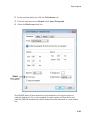
To insert a function:
1-8
1
Point the cursor at the place in an input region where you want to insert a function.
2
Click the button corresponding to the function.
3
Insert the parameters instead of the # symbols. You can switch between the
parameters by pressing the Tab key.
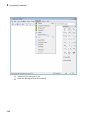
Shortcut to Access Standard MuPAD Functions
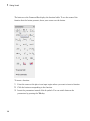
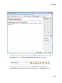
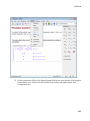
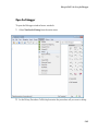
Most of the buttons on the Command Bar include a drop-down menu with a list of similar
functions. The buttons display a small triangle in the bottom right corner. Click the
button to open the list of functions.
1-9
1
Getting Started
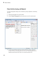
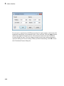
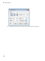
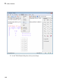
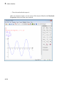
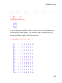
Using the Command Bar, you also can create the following:
• Vectors and matrices
1-10
Shortcut to Access Standard MuPAD Functions
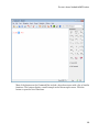
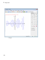
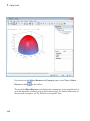
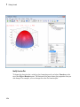
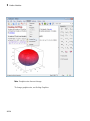
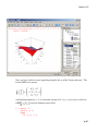
• 2-D plots and animations
1-11
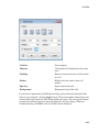
1
Getting Started
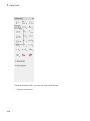
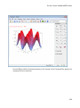
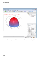
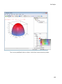
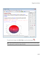
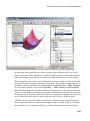
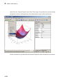
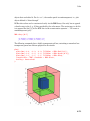
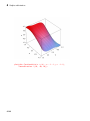
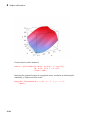
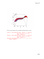
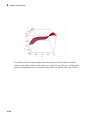
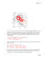
• 3-D plots
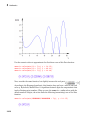
1-12
Shortcut to Access Standard MuPAD Functions
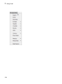
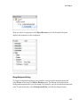
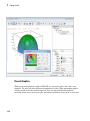
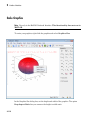
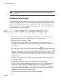
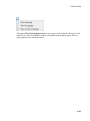
General Math and Plot Commands menus at the bottom of the Command Bar display the
categorized lists of functions.
1-13
1
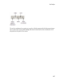
Getting Started
1-14
Access Help for Particular Command
Access Help for Particular Command
Note: Use only in the MuPAD Notebook Interface. This functionality does not run in
MATLAB.
In this section...
“Autocomplete Commands” on page 1-15
“Use Tooltips and the Context Menu” on page 1-16
“Use Help Commands” on page 1-18
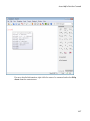
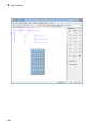
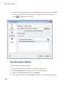
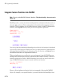
Autocomplete Commands
MuPAD helps you complete the names of known commands as you type them so that
you can avoid spelling mistakes. Type the first few characters of the command name,
and then press Ctrl+space. If there is exactly one name of a command that starts with
these letters, MuPAD completes the command. If more than one name starts with the
characters you typed, MuPAD displays a list of all names starting with those characters.
1-15
1
Getting Started
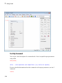
Use Tooltips and the Context Menu
To get a brief description and acceptable syntax for a function, type the function name in
a notebook and hover your cursor over the command.
1-16
Access Help for Particular Command
For more detailed information, right-click the name of a command and select Help
about from the context menu.
1-17
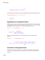
1
Getting Started
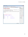
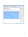
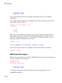
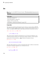
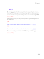
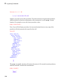
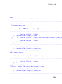
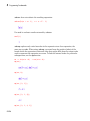
Use Help Commands
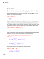
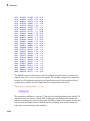
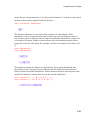
You can get a brief description of a command and a list of acceptable input parameters
using info:
info(solve)
solve -- solve equations and inequalities [try ?solve for options]
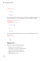
For more detailed information about the command and its input parameters, use the ?
command:
?solve
1-18
Perform Computations
Perform Computations
Note: Use only in the MuPAD Notebook Interface. This functionality does not run in
MATLAB.
In this section...
“Compute with Numbers” on page 1-19
“Differentiation” on page 1-23
“Integration” on page 1-26
“Linear Algebra” on page 1-27
“Solve Equations” on page 1-31
“Manipulate Expressions” on page 1-33
“Use Assumptions in Your Computations” on page 1-36
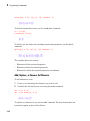
Compute with Numbers
Types of Numbers
Using MuPAD, you can operate on the following types of numbers:
• Integer numbers
• Rational numbers
• Floating-point numbers
• Complex numbers
By default, MuPAD assumes that all variables are complex numbers.
Compute with Integers and Rationals
When computing with integers and rational numbers, MuPAD returns integer results
2 + 2
1-19
1
Getting Started
or rational results:
(1 + (5/2*3))/(1/7 + 7/9)^2
If MuPAD cannot find a representation of an expression in an integer or rational form, it
returns a symbolic expression:
56^(1/2)
Compute with Special Mathematical Constants
You can perform exact computations that include the constants =exp(1)=2.718...
and π=3.1415...:
2*(exp(2)/PI)
For more information on the mathematical constants implemented in MuPAD, see
“Constants”.
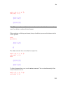
Approximate Numerically
By default, MuPAD performs all computations in an exact form. To obtain a floatingpoint approximation to an expression, use the float command. For example:
float(sqrt(56))
The accuracy of the approximation depends on the value of the global variable DIGITS.
The variable DIGITS can assume any integer value between 1 and 229 + 1. For example:
DIGITS:=20: float(sqrt(56))
1-20
Perform Computations
The default value of the variable DIGITS is 10. To restore the default value, enter:
delete DIGITS
When MuPAD performs arithmetic operations on numbers involving at least one
floating-point number, it automatically switches to approximate numeric computations:
(1.0 + (5/2*3))/(1/7 + 7/9)^2
If an expression includes exact values such as
MuPAD approximates only numbers:
or sin(2) and floating-point numbers,
1.0/3*exp(1)*sin(2)
To approximate an expression with exact values, use the float command:
float(1.0/3*exp(1)*sin(2))
or use floating-point numbers as arguments:
1.0/3*exp(1.0)*sin(2.0)
You also can approximate the constants π and :
DIGITS:=30: float(PI); float(E); delete DIGITS
1-21
1
Getting Started
Work with Complex Numbers
In the input regions MuPAD recognizes an uppercase I as the imaginary unit
. In
the output regions, MuPAD uses a lowercase i to display the imaginary unit:
sqrt(-1), I^2
Both real and imaginary parts of a complex number can contain integers, rationals, and
floating-point numbers:
(1 + 0.2*I)*(1/2 + I)*(0.1 + I/2)^3
If you use exact expressions, for example,
in Cartesian coordinates:
, MuPAD does not always return the result
1/(sqrt(2) + I)
To split the result into its real and imaginary parts, use the rectform command:
rectform(1/(sqrt(2) + I))
The functions Re and Im return real and imaginary parts of a complex number:
Re(1/(2^(1/2) + I))
1-22
Perform Computations
Im(1/(2^(1/2) + I))
The function conjugate returns the complex conjugate:
conjugate(1/(2^(1/2) + I))
The function abs and arg return an absolute value and a polar angle of a complex
number:
abs(1/(2^(1/2) + I));
arg(1/(2^(1/2) + I))
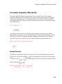
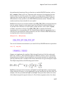
Differentiation
Derivatives of Single-Variable Expressions
To compute the derivative of a mathematical expression, use the diff command. For
example:
f := 4*x + 6*x^2 + 4*x^3 + x^4: diff(f, x)
Partial Derivatives
You also can compute a partial derivative of a multivariable expression:
1-23
1
Getting Started
f := y^2 + 4*x + 6*x^2 + 4*x^3 + x^4: diff(f, y)
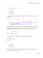
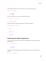
Second- and Higher-Order Derivatives
To find higher order derivatives, use a nested call of the diff command
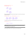
diff(diff(diff(sin(x), x), x), x)
or, more efficiently:
diff(sin(x), x, x, x)
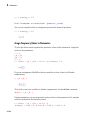
You can use the sequence operator $ to compute second or higher order derivatives:
diff(sin(x), x $ 3)
Mixed Derivatives
diff(f, x1, x2, ...) is equivalent to diff(...diff(diff(f, x1), x2)...).
The system first differentiates f with respect to x1, and then differentiates the result
with respect to x2, and so on. For example
diff(diff((x^2*y^2 + 4*x^2*y + 6*x*y^2), y), x)
is equivalent to
diff(x^2*y^2 + 4*x^2*y + 6*x*y^2, y, x)
1-24
Perform Computations
Note: To improve performance, MuPAD assumes that all mixed derivatives commute.
For example,
.
This assumption suffices for most of engineering and scientific problems.
For further computations, delete f:
delete f:
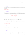
Derivatives of a Function
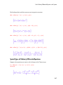
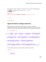
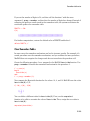
MuPAD provides two differentiation functions, diff and D. The diff function serves for
differentiating mathematical expressions, such as sin(x), cos(2y), exp(x^2), x^2 +
1, f(y), and so on.
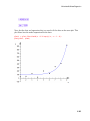
To differentiate a standard function, such as sin, exp, heaviside, or a custom function,
such as f:= x -> x^2 + 1, use the differential operator D:
D(sin), D(exp), D(heaviside)
f := x -> x^2 + 1: D(f)
' is a shortcut for the differential operator D:
sin', sin'(x), f'
The command D(f)(x) assumes that f is a univariate function, and represents the
derivative of f at the point x. For example, the derivative of the sine function at the point
x2 is:
D(sin)(x^2)
1-25
1
Getting Started
Note that in this example you differentiate the sin function, not the function f := x ->
sin(x^2). Differentiating f returns this result:
f := x -> sin(x^2): D(f)
For details about using the operator D for computing second- and higher-order
derivatives of functions, see Differentiating Functions.
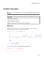
Integration
Indefinite Integrals
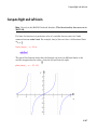
To compute integrals use the int command. For example, you can compute indefinite
integrals:
int((cos(x))^3, x)
The int command returns results without an integration constant.
Definite Integrals
To find a definite integral, pass the upper and lower limits of the integration interval to
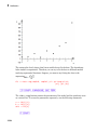
the int function:
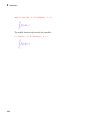
int((cos(x))^3, x = 0..PI/4)
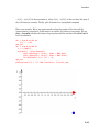
You can use infinity as a limit when computing a definite integral:
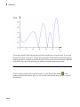
int(sin(x)/x, x = -infinity..infinity)
1-26
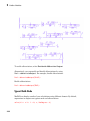
Perform Computations
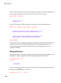
Numeric Approximation
If MuPAD cannot evaluate an expression in a closed form, it returns the expression. For
example:
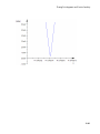
int(sin(x^2)^2, x = -1..1)
You can approximate the value of an integral numerically using the float command.
For example:
float(int(sin(x^2)^2,(x = -1..1)))
You also can use the numeric::int command to evaluate an integral numerically. For
example:
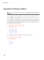
numeric::int(sin(x^2)^2, x = -1..1)
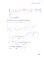
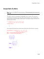
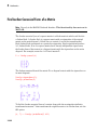
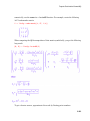
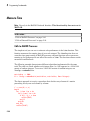
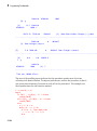
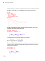
Linear Algebra
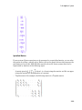
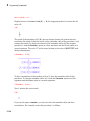
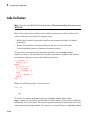
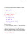
Create a Matrix
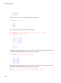
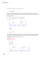
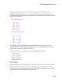
To create a matrix in MuPAD, use the matrix command:
A := matrix([[1, 2], [3, 4], [5, 6]]);
B := matrix([[1, 2, 3], [4, 5, 6]])
1-27
1
Getting Started
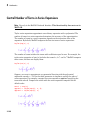
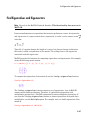
You also can create vectors using the matrix command:
V := matrix([1, 2, 3])
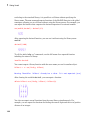
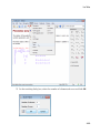
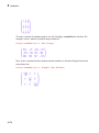
You can explicitly declare the matrix dimensions:
C := matrix(3, 3, [[-1, -2, -3], [-4, -5, -6], [-7, -8, -9]]);
W := matrix(1, 3, [1, 2, 3])
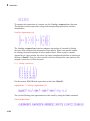
If you declare matrix dimensions and enter rows or columns shorter than the declared
dimensions, MuPAD pads the matrix with zero elements:
F := matrix(3, 3, [[1, -1, 0], [2, -2]])
If you declare matrix dimensions and enter rows or columns longer than the declared
dimensions, MuPAD returns the following error message:
matrix(3, 2, [[-1, -2, -3], [-4, -5, -6], [-7, -8, -9]])
1-28
Perform Computations
Error: The number of columns does not match. [(Dom::Matrix(Dom::ExpressionField()))::mk
You also can create a diagonal matrix:
G := matrix(4, 4, [1, 2, 3, 4], Diagonal)
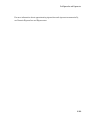
Operate on Matrices
To add, substract, multiply and divide matrices, use standard arithmetic operators. For
example, to multiply two matrices, enter:
A := matrix([[1, 2], [3, 4], [5, 6]]);
B := matrix([[1, 2, 3], [4, 5, 6]]);
A*B
If you add number x to a matrix A, MuPAD adds x times an identity matrix to A. For
example:
C := matrix(3, 3, [[-1, -2, -3], [-4, -5, -6], [-7, -8, -9]]);
C + 10
1-29
1
Getting Started
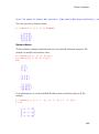
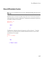
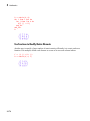
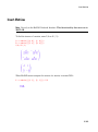
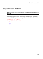
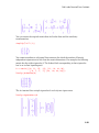
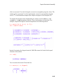
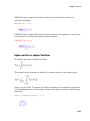
You can compute the determinant and the inverse of a square matrix:
G := matrix([[1, 2, 0], [2, 1, 2], [0, 2, 1]]); det(G); 1/G
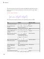
Linear Algebra Library
The MuPAD linalg library contains the functions for handling linear algebraic
operations. Using this library, you can perform a wide variety of computations on
matrices and vectors. For example, to find the eigenvalues of the square matrices G, F,
and (A*B), use the linalg::eigenvalue command:
linalg::eigenvalues(G);
linalg::eigenvalues(F);
linalg::eigenvalues(A*B)
1-30
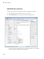
Perform Computations
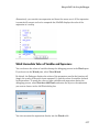
To see all the functions available in this library, enter info(linalg) in an input
region. You can obtain detailed information about a specific function by entering ?
functionname. For example, to open the help page on the eigenvalue function, enter ?
linalg::eigenvalues.
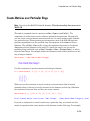
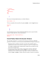
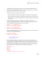
Solve Equations
Solve Equations with One Variable
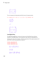
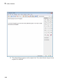
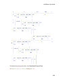
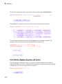
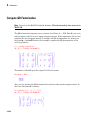
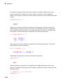
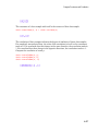
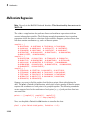
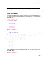
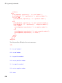
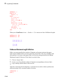
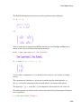
To solve a simple algebraic equation with one variable, use the solve command:
solve(x^5 + 3*x^4 - 23*x^3 - 51*x^2 + 94*x + 120 = 0, x)
Solving Equations with Parameters
You can solve an equation with symbolic parameters:
solve(a*x^2 + b*x + c = 0, x)
If you want to get the solution for particular values of the parameters, use the assuming
command. For example, you can solve the following equation assuming that a is positive:
solve(a*x^2 + b*x + c = 0, x) assuming a > 0
1-31
1
Getting Started
For more information, see Using Assumptions.
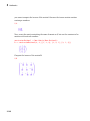
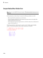
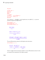
Solve Systems of Equations
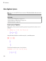
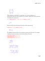
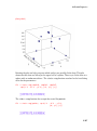
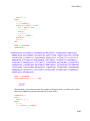
You can solve a system of equations:
solve([x^2 + x*y + y^2 = 1, x^2 - y^2 = 0], [x, y])
or you can solve a system of equations containing symbolic parameters:
solve([x^2 + y^2 = a, x^2 - y^2 = b], [x, y])
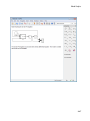
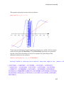
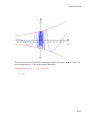
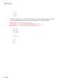
Solve Ordinary Differential Equations
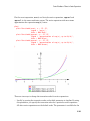
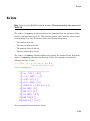
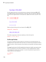
You can solve different types of ordinary differential equations:
o := ode(x^2*diff(y(x), x, x) + 2*x*diff(y(x), x) + x, y(x)):
solve(o)
1-32
Perform Computations
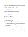
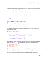
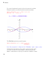
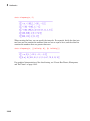
Solve Inequalities
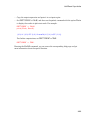
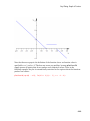
Also, you can solve inequalities:
solve(x^4 >= 5, x)
If you want to get the result over the field of real numbers only, assume that x is a real
number:
assume(x in R_); solve(x^4 >= 5, x)
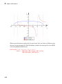
You can pick the solutions that are positive:
solve(x^4 >= 5, x) assuming x > 0
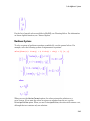
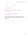
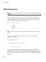
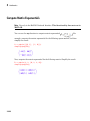
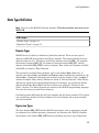
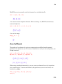
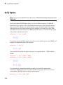
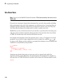
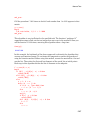
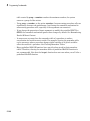
Manipulate Expressions
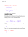
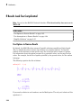
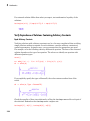
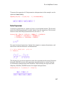
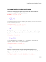
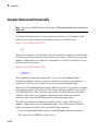
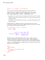
Transform and Simplify Polynomial Expressions
There are several ways to present a polynomial expression. The standard polynomial
form is a sum of monomials. To get this form of a polynomial expression, use the expand
command:
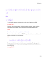
expand((x - 1)*(x + 1)*(x^2 + x + 1)*
(x^2 + 1)*(x^2 - x + 1)*(x^4 - x^2 + 1))
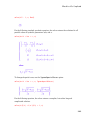
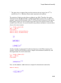
You can factor this expression using the factor command:
factor(x^12 - 1)
1-33
1
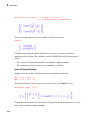
Getting Started
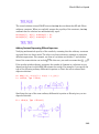
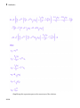
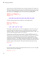
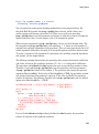
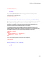
For multivariable expressions, you can specify a variable and collect the terms with the
same powers in this variable:
collect((x - a)^4 + a*x^3 + b^2*x + b*x + 10*a^4 +
(b + a*x)^2, x)
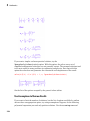
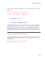
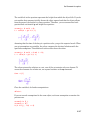
For rational expressions, you can use the partfrac command to present the expression
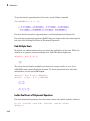
as a sum of fractions (partial fraction decomposition). For example:
partfrac((7*x^2 + 7*x + 6)/(x^3 + 2*x^2 + 2*x + 1))
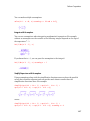
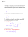
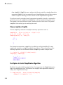
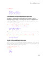
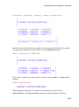
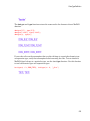
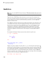
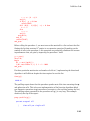
MuPAD also provides two general simplification functions: simplify and Simplify.
The simplify function is faster and it can handle most of the elementary expressions:
simplify((x - 1)*(x + 1)*(x^2 + x + 1)*(x^2 + 1)*
(x^2 - x + 1)*(x^4 - x^2 + 1))
The Simplify function searches for simpler results deeper than the simplify function.
The more extensive search makes this function slower than simplify. The Simplify
function allows you to extend the simplification rule set with your own rules and serves
better for transforming more complex expressions. For the elementary expressions it
gives the same result as simplify:
Simplify((x - 1)*(x + 1)*(x^2 + x + 1)*(x^2 + 1)*
(x^2 - x + 1)*(x^4 - x^2 + 1))
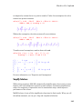
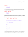
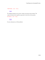
For the following expression the two simplification functions give different forms of the
same mathematical expression:
1-34
Perform Computations
f := exp(wrightOmega(-ln(3/5)))*exp(ln(5) - ln(3)):
simplify(f);
Simplify(f)
Note that there is no universal simplification strategy, because the meaning of the
simplest representation of a symbolic expression cannot be defined clearly. Different
problems require different forms of the same mathematical expression. You can use the
general simplification functions simplify and Simplify to check if they give a simpler
form of the expression you use.
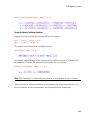
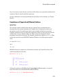
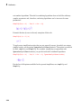
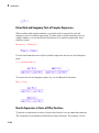
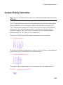
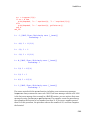
Transform and Simplify Trigonometric Expressions
You also can transform and simplify trigonometric expressions. The functions for
manipulating trigonometric expressions are the same as for polynomial expressions. For
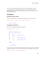
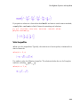
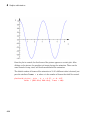
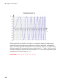
example, to expand a trigonometric expression, use the expand command:
expand(sin(5*x))
To factor the trigonometric expression, use the factor command:
factor(cos(x)^4 + 4*cos(x)^3*sin(x) + 6*cos(x)^2*sin(x)^2 +
4*cos(x)*sin(x)^3 + sin(x)^4)
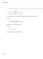
You can use the general simplification functions on trigonometric expressions:
simplify(cos(x)^2 + sin(x)^2)
1-35
1
Getting Started
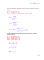
simplify(cos(x)^4 + sin(x)^4 + sin(x)*cos(x))
Simplify(cos(x)^4 + sin(x)^4 + sin(x)*cos(x))
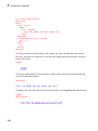
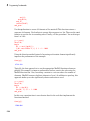
Use Assumptions in Your Computations
Solve Expressions with Assumptions
By default, all variables in MuPAD represent complex numbers. When solving equations
or simplifying expressions, the software considers all possible cases for complex numbers.
If you are solving an equation or simplifying an expression, this default assumption leads
to the exact and complete set of results including complex solutions:
solve(x^(5/2) = 1, x)
To obtain real solutions only, pass the assumption to MuPAD using the assuming
command:
solve(x^(5/2) = 1, x) assuming x in R_
You can make various assumptions on the values that a variable represents. For
example, you can solve an equation assuming that the variable x represents only positive
values:
solve(x^4 - 1 = 0, x) assuming x > 0
1-36
Perform Computations
You can make multiple assumptions:
solve(x^4 - a = 0, x) assuming a = 16 and x in R_
Integrate with Assumptions
You can use assumptions when integrating mathematical expressions. For example,
without an assumption on the variable x, the following integral depends on the sign of
the expression x2 - 1:
int(1/abs(x^2 - 1), x)
If you know that x > 1, you can pass the assumption to the integral:
int(1/abs(x^2 - 1), x) assuming x > 1
Simplify Expressions with Assumptions
Using assumptions along with the simplification functions narrows down the possible
values that variables represent and can provide much shorter results than the
simplification functions alone. For example:
simplify(sqrt(x^2 + 2*x + 1) + sqrt(x^2 - 2*x + 1) +
sqrt(x^2 + 4*x + 4) + sqrt(x^2 - 4*x + 4))
versus
simplify(sqrt(x^2 + 2*x + 1) + sqrt(x^2 - 2*x + 1) +
sqrt(x^2 + 4*x + 4) + sqrt(x^2 - 4*x + 4)) assuming x > 2
1-37
1
Getting Started
You can pass assumptions to the following functions: expand, simplify, limit, solve,
and int. The Simplify function does not allow assumptions on variables.
1-38
Use Graphics
Use Graphics
Note: Use only in the MuPAD Notebook Interface. This functionality does not run in
MATLAB.
In this section...
“Graphic Options Available in MuPAD” on page 1-39
“Basic Plotting” on page 1-40
“Format Plots” on page 1-49
“Present Graphics” on page 1-56
“Create Animated Graphics” on page 1-59
Graphic Options Available in MuPAD
Basic Plotting Options
MuPAD presents many options for creating and working with graphics and animations.
The simplest way to create a plot in MuPAD is to use the plot command. Using this
command, you can:
• Create 2-D and 3-D function plots
• Specify plotting range
• Create plots for piecewise functions
• Create multiple function plots in one graph
• Create animated 2-D and 3-D function plots
You can format the plot interactively.
Advanced Plotting Options
The plot command provides a basic way to create function plots. For example, you can:
• Create a 2-D function plot using plot::Function2d.
• Create a 3-D function plot using plot::Function3d.
• Create animated plots.
1-39
1
Getting Started
• Create function plots in polar or spherical coordinates.
• Create turtle graphics and Lindenmayer systems.
• Choose colors, fonts, legends, axes appearance, grid lines, tick marks, line, and
marker styles.
• Apply affine transformations to a plot. You can scale, rotate, reflect, or move a plot.
• Set cameras for a 3-D plot.
• See the MuPAD gallery of plots.
To see all functions available in the MuPAD graphics library, enter:
info(plot)
Basic Plotting
Create 2-D Plots
The simple way to create a 2-D plot of a function is to use the plot command:
plot(sin(x)*cos(3*x))
1-40
Use Graphics
Create 3-D Plots
The simple way to create a 3-D plot of a function is to use the plot command with the
option #3D:
plot(sin(x)*sin(y), #3D)
Note: By default, for a function of two variables, the plot command creates a 2-D
animation. Using the option #3D lets you create a 3-D plot instead of a 2-D animation.
Plot Multiple Functions in One Graph
To plot several functions in one figure, list all the functions, separating them by commas.
MuPAD uses different colors when plotting multiple functions:
plot(sin(x), cos(x), tan(x), cot(x))
1-41
1
Getting Started
You can use the sequence generator $ to create a sequence of functions:
plot(sin(k*x) $ k = 1..3)
1-42
Use Graphics
You also can plot multiple functions in one 3-D graph:
plot(-sqrt(r^2 - x^2 - y^2) $ r = 1..5, #3D)
1-43
1
Getting Started
Specify Plot Ranges
You can specify a range over which to plot a function:
plot(sin(x^3)*exp(x), x = 3..5)
1-44
Use Graphics
plot(sin(x)*sin(y), x = 0..3, y = 1..3, #3D)
1-45
1
Getting Started
For multiple functions plotted in one graph, you can specify one range for all the
functions:
plot(sin(k*x) $ k = 1..5, x = 0..2*PI)
1-46
Use Graphics
To specify different ranges for multiple functions plotted in one graph, use different
variables:
plot({sin(k*x), k*t^2} $ k = 1..5, x = 0..2*PI, t = -1..1)
1-47
1
Getting Started
Plot Piecewise Functions
To specify a piecewise function, use the piecewise command. You can plot a piecewise
function even if it is undefined at some points. for example, you can plot the following
function although the function is not defined for -2 < x < -1:
plot(piecewise([x < - 2, - 1], [-1 < x and x < 0, x^2],
[0 < x and x < 1, -x^2], [x > 1, 1]))
1-48
Use Graphics
Format Plots
Enable Plot Formatting Mode
In MuPAD, you can format your graphic results interactively when working in plot
formatting mode. To switch to graphics formatting mode, click any place on a plot. In this
mode, the Object Browser pane appears.
1-49
1
Getting Started
If you do not see the Object Browser and Property panes, select View > Object
Browser or click
on the toolbar.
The top of the Object Browser pane displays the components of your graphics such as
scene (background), coordinate system, and a function plot. For further information on
the structure of graphics, see The Full Picture: Graphical Trees.
1-50
Use Graphics
After you select a component in the Object Browser pane, the bottom of the pane
displays the properties of this component.
Change Background Settings
To change background settings of your graphics, switch to plot formatting mode and
select Scene at the top of the Object Browser pane. The bottom of the pane shows
background properties that you can change. For example, you can change the background
color. To choose the color, select BackgroundColor and click the ellipsis button.
1-51
1
Getting Started
You can use predefined colors or select a color from a more extensive palette.
1-52
Use Graphics
Modify Axes
To format the axes of your graphics, switch to plot formatting mode and select
Coordinate System at the top of the Object Browser pane. The bottom of the pane
shows axes properties that you can change. For example, you can add grid lines.
1-53
1
Getting Started
Modify Function Plot
To format the function plot, switch to plot formatting mode and select Function at the
top of the Object Browser pane. The bottom of the pane shows plot properties that you
can change. For example, you can change the color of a function plot.
1-54
Use Graphics
You can use predefined colors or select a color from a more extensive palette.
1-55
1
Getting Started
Present Graphics
When you present graphic results in MuPAD, you can move, zoom, and rotate your
graphics. You also can select different components of a plot. When presenting graphic
results, switch to the plot formatting mode. You can use the following toolbar to
manually rotate, move, zoom your plot, and show coordinates of any point on your plot:
1-56
Use Graphics
To see the coordinates for a point on your plot, click the point and hold the mouse button.
You can move the cursor while holding the mouse button and see the coordinates of all
the points on the path of the cursor.
1-57
1
Getting Started
You can use the toolbar to rotate and zoom your plot automatically. You also can change
the speed for rotation and zooming.
1-58
Use Graphics
Create Animated Graphics
Creating Animated 2-D Plots
To create an animated plot, use an additional changing parameter for the function you
want to plot. Specify the range for this parameter. The following example presents an
animated plot of a function with the parameter a that gradually changes value from 2 to
6:
plot(exp(x)*sin(a^2*x), x = 1..2, a = 2..6)
Create Animated 3-D Plots
To create an animated 3-D plot, use an additional changing parameter for the function
you want to plot. Specify the range for this parameter and the option #3D. The following
example presents an animated plot of a function with the parameter a that gradually
changes value from 0.1 to 2:
plot(sin(a*x^2 + a*y^2), x = -2..2, y = -2..2, a = 0.1..2, #3D)
1-59
1
Getting Started
Play Animations
MuPAD displays the first frame of an animation as static picture. To play the animation,
click the picture.
When MuPAD plays an animation, the Animation toolbar with the player controls
appears:
1-60
Use Graphics
Count Backwards
To play an animation forward and then backward, click the Repetition button
select the option Back and Forth.
and
You also can specify the range for a parameter so that the initial value is greater than
the final value. The following example creates an animated plot of the function using the
parameter a that gradually changes value from 2 to 0.1:
plot(sin(a*x^2 + a*y^2), x = -2..2, y = -2..2, a = 2..0.1, #3D)
1-61
1
Getting Started
Use the MuPAD Libraries
Note: Use only in the MuPAD Notebook Interface. This functionality does not run in
MATLAB.
In this section...
“Overview of Libraries” on page 1-62
“Standard Library” on page 1-63
“Find Information About a Library” on page 1-64
“Avoid Name Conflicts Between MuPAD Objects and Library Functions” on page
1-65
Overview of Libraries
Libraries contain most of the MuPAD functionality. Each library includes a collection of
functions for solving particular types of mathematical problems:
1-62
combinat
supports combinatorics operations
solvelib
contains various methods used by the
function solve
export
supports exporting MuPAD data to
external formats
output
supports formatted output of the MuPAD
data
fp
supports functional programming methods
generate
supports conversion of the MuPAD
expressions to C, FORTRAN, MATLAB®,
and TeX codes
groebner
supports operating on ideals of multivariate
polynomial rings over a field
import
supports importing external data to
MuPAD
Use the MuPAD Libraries
transform
supports integral transformations and the
discrete Z-transform
intlib
supports manipulating and solving
integrals
linalg
supports linear algebra operations
linopt
provides algorithms for linear and integer
programming
listlib
supports manipulating lists
polylib
supports manipulating polynomials
stringlib
supports manipulating strings
numlib
supports number theory operations
numeric
provides algorithms for numeric
mathematics
ode
supports manipulating and solving
ordinary differential equations
orthpoly
provides a set of standard orthogonal
polynomials
Pref
supports setting and restoring user
preferences
prog
provides programming utilities for
analyzing functions and tracing errors
stats
provides methods for statistical analysis
Type
supports checking types of MuPAD objects
Symbol
supports typesetting symbols
Functions included in libraries are written in the MuPAD language. The calling syntax
for functions from all the libraries (except for the standard library) includes both the
library name and the function name: library::function.
Standard Library
The standard library presents the set of most frequently used functions including diff,
int, simplify, solve, and other functions. For example:
diff(x^2,x)
1-63
1
Getting Started
Find Information About a Library
You can get information about the libraries using the info and help commands. The
info command gives a list of functions of a particular library. For example, the numlib
library presents a collection of functions for number theory operations:
info(numlib)
Library 'numlib': the package for elementary number theory
-- Interface:
numlib::Lambda,
numlib::Omega,
numlib::checkPrimalityCertificate, numlib::contfrac,
1-64
numlib::contfracPeriodic,
numlib::cornacchia,
numlib::decimal,
numlib::divisors,
numlib::factorGaussInt,
numlib::fibonacci,
numlib::fromAscii,
numlib::g_adic,
numlib::ichrem,
numlib::igcdmult,
numlib::invphi,
numlib::ispower,
numlib::isquadres,
numlib::issqr,
numlib::jacobi,
numlib::lambda,
numlib::legendre,
numlib::lincongruence,
numlib::mersenne,
numlib::moebius,
numlib::mroots,
numlib::msqrts,
numlib::numdivisors,
numlib::numprimedivisors,
numlib::omega,
numlib::order,
numlib::phi,
numlib::pi,
Use the MuPAD Libraries
numlib::primedivisors,
numlib::primroot,
numlib::proveprime,
numlib::reconstructRational,
numlib::sigma,
numlib::sqrt2cfrac,
numlib::sqrtmodp,
numlib::sumOfDigits,
numlib::sumdivisors,
numlib::tau,
numlib::toAscii,
To see brief information about a particular library function, use the mouse pointer to
hover the cursor over the function name.
For more information about the library and for information about the library functions,
enter:
?numlib
To see the implementation of a library function, use the expose command:
expose(numlib::tau)
proc(a)
name numlib::tau;
begin
if args(0) <> 1 then
error(message("symbolic:numlib:IncorrectNumberOfArguments"))
else
if not testtype(a, Type::Numeric) then
return(procname(args()))
else
if domtype(a) <> DOM_INT then
error(message("symbolic:numlib:ArgumentInteger"))
end_if
end_if
end_if;
numlib::numdivisors(a)
end_proc
Avoid Name Conflicts Between MuPAD Objects and Library Functions
You can call any library function (except for the standard library functions) using the
following syntax: library::function. If you frequently use some functions that do
1-65
1
Getting Started
not belong to the standard library, it is possible to call them without specifying the
library name. The use command exports functions of the MuPAD libraries to the global
namespace allowing you to call them without using the library names. For example, you
can export the function that computes the decimal expansion of a rational number:
use(numlib,decimal): decimal(1/3)
After exporting the decimal function, you can use it without using the library name
numlib:
decimal(1/200)
To call the info, help, or ? commands, use the full name of an exported function
including the name of a library:
?numlib::decimal
You cannot export a library function with the same name you use for another object:
hilbert := x: use(linalg, hilbert)
Warning: Identifier 'hilbert' already has a value. It is not exported. [use]
After clearing the variable decimal, you can export a function:
delete hilbert: use(linalg, hilbert): hilbert(3)
You also can export several functions from the same library simultaneously. For
example, you can export the functions for finding the sum of digits and the set of positive
divisors of an integer:
1-66
Use the MuPAD Libraries
use(numlib, sumOfDigits, numdivisors): numdivisors(21); sumOfDigits(21)
To export all functions of a library, pass the library name to the use command. If some of
the library functions have name conflicts with other objects, the use command issues a
warning for each name conflict:
use(numeric)
Warning: Identifier 'product' already has a value. It is not exported. [use]
Warning: Identifier 'int' already has a value. It is not exported. [use]
Warning: Identifier 'indets' already has a value. It is not exported. [use]
Warning: Identifier 'det' already has a value. It is not exported. [use]
Warning: Identifier 'linsolve' already has a value. It is not exported. [use]
Warning: Identifier 'rationalize' already has a value. It is not exported. [use]
Warning: Identifier 'inverse' already has a value. It is not exported. [use]
Warning: Identifier 'solve' already has a value. It is not exported. [use]
Warning: Identifier 'sum' already has a value. It is not exported. [use]
Warning: Identifier 'sort' already has a value. It is not exported. [use]
These library functions have the same names as the standard library functions. You
cannot delete standard library functions and resolve the name conflicts. Use the full
function names such as numeric::product to call these functions.
1-67
2
Notebook Interface
• “Notebook Overview” on page 2-3
• “Debugger Window Overview” on page 2-5
• “Arrange Toolbars and Panes” on page 2-8
• “Enter Data and View Results” on page 2-11
• “View Status Information” on page 2-13
• “Save Custom Arrangements” on page 2-14
• “Format Text” on page 2-15
• “Format Mathematical Expressions” on page 2-21
• “Format Expressions in Input Regions” on page 2-24
• “Change Default Format Settings” on page 2-28
• “Use Frames” on page 2-32
• “Use Tables” on page 2-38
• “Embed Graphics” on page 2-45
• “Work with Links” on page 2-48
• “Export Notebooks to HTML, PDF, and Plain Text Formats” on page 2-59
• “Save and Export Graphics” on page 2-61
• “Set Preferences for Notebooks” on page 2-71
• “Set Preferences for Dialogs, Toolbars, and Graphics” on page 2-75
• “Set Font Preferences” on page 2-79
• “Set Engine Preferences” on page 2-82
• “Get Version Information” on page 2-86
• “Use Different Output Modes” on page 2-87
• “Set Line Length in Plain Text Outputs” on page 2-94
• “Delete Outputs” on page 2-95
• “Greek Letters in Text Regions in MuPAD” on page 2-96
2
Notebook Interface
• “Special Characters in Outputs” on page 2-97
• “Non-Greek Characters in Text Regions” on page 2-98
• “Use Keyboard Shortcuts” on page 2-99
• “Use Mnemonics” on page 2-101
• “Wrap Long Lines” on page 2-102
• “Hide Code Lines” on page 2-110
• “Change Font Size Quickly” on page 2-113
• “Scale Graphics” on page 2-116
• “Use Print Preview” on page 2-118
• “Change Page Settings for Printing” on page 2-122
• “Print Wide Notebooks” on page 2-123
2-2
Notebook Overview
Notebook Overview
Note: Use only in the MuPAD Notebook Interface. This functionality does not run in
MATLAB.
The first time you start MuPAD notebook, it appears with the default layout, as shown in
the following illustration.
• A Perform most common tasks from the Standard toolbar.
2-3
2
Notebook Interface
• B Type your comments in the text regions.
• C Enter commands in the input regions.
• D View results (including graphics) in the output regions.
• E A new input region appears after evaluation of the bottom input region.
• F View current status information in the Status bar.
• G Find and Replace text in the input and text regions.
• H Quickly access standard functions from the Command Bar.
• I Format nongraphical objects in the input and output regions from the Format
toolbar.
• J Use more items from the toolbars.
• K Menus change in the Graphics Format mode.
2-4
Debugger Window Overview
Debugger Window Overview
Note: Use only in the MuPAD Notebook Interface. This functionality does not run in
MATLAB.
The first time you start MuPAD Debugger window, it appears with the default layout, as
shown in the following illustration.
2-5
2
Notebook Interface
• A Perform common tasks from the toolbar.
• B View the code that you debug.
2-6
Debugger Window Overview
• C Type an expression and evaluate it in the Output pane anytime during the
debugging process.
• D Use the Status bar to view memory and time usage for the current or most recent
debugging step.
• E Use the Watch pane to view values of variables during the debugging process.
• F Use the Call Stack pane to view the names of the procedures participating in the
debugging process.
For information about the Debugger mode, see Tracing Errors with the Debugger.
2-7
2
Notebook Interface
Arrange Toolbars and Panes
Note: Use only in the MuPAD Notebook Interface. This functionality does not run in
MATLAB.
In this section...
“Enabling and Disabling Toolbars and Panes” on page 2-8
“Move Toolbars and Panes” on page 2-9
Enabling and Disabling Toolbars and Panes
To enable or disable the Command Bar, Find and Replace Bar, toolbars, or Status Bar,
select View from the main menu. The following illustration shows the View menu for a
notebook and a Debugger window.
To use context menu, right-click any bar. The following illustration shows the context
menu for the Notebook and Debugger windows.
2-8
Arrange Toolbars and Panes
Move Toolbars and Panes
To move a toolbar, grab the toolbar anchor and drag the toolbar to a different location.
For example, line the toolbars one below the other.
To move the Command Bar or Find and Replace Bar, grab the pane title and drag the
pane to a different location. For example, move the Command Bar to the left.
2-9
2
Notebook Interface
2-10
Enter Data and View Results
Enter Data and View Results
Note: Use only in the MuPAD Notebook Interface. This functionality does not run in
MATLAB.
MuPAD notebook has two types of regions for entering data:
• Text regions serve for entering your comments. They can contain text, tables,
mathematical formulas, and graphics. Text regions do not have not bracket markers.
The default font color for text regions is black. To start a new text region, click outside
the gray brackets and start typing. Alternatively, you can insert a new text region by
selecting Insert>Text Paragraph or Insert>Text Paragraph Above. You cannot
insert a text region inside a region of other type or between adjacent input and output
regions.
• Input regions serve for entering your code. They can contain MuPAD
mathematical expressions and commands in the MuPAD language. Input regions
have gray bracket markers. The default font color for input regions is red. When
you evaluate an expression in the bottom input region, MuPAD inserts a new
input region below. To insert new input regions in other parts of a notebook,
select Insert>Calculation or Insert>Calculation Above from the main menu.
Alternatively, use the Insert Calculation button
.
MuPAD notebook has a special type of region for viewing results:
• Output regions serve for viewing results. These regions automatically appear when
you evaluate input regions. The results can include graphics and error messages.
The default font color for output regions is blue. You cannot edit data in the output
regions. To change the results, edit the associated input region and evaluate it by
pressing Enter. Also, you can copy results from the output regions to the text and
input regions. When you copy outputs to the input regions, MuPAD inserts ASCII
equivalents of the results in the input regions.
If you want to change the default text color, font, or the appearance of brackets for the
current notebook, see Changing Default Format Settings.
If you want to change preferences for all notebooks, see Setting Preferences for
Notebooks.
2-11
2
Notebook Interface
Note: Most preferences affect only new notebooks. They do not affect existing notebooks.
2-12
View Status Information
View Status Information
Note: Use only in the MuPAD Notebook Interface. This functionality does not run in
MATLAB.
The status bar shows the current status information.
• A Displays memory and time usage for the current or most recent computation.
• B Indicated the type of the currently active region.
• C Indicates insert or overwrite mode.
View the current engine state at the far left end of the status bar. If the engine is not
connected to your notebook, the status bar displays Not Connected.
The status bar indicates the type of the region where you position the cursor. The
indicator displays:
• Cmd, if the cursor is in an input region
• Text, if the cursor is in a text region
• Outp, if the cursor is in an output region
The status bar also indicates if the cursor is in a read-only part of a notebook, for
example, in an output region.
For text and input regions, MuPAD notebook supports overwrite mode. Press the Insert
key to enter text in overwrite mode. Press the Insert key again to return to entering text
in insert mode. View the current state at the far right of the status bar.
2-13
2
Notebook Interface
Save Custom Arrangements
Note: Use only in the MuPAD Notebook Interface. This functionality does not run in
MATLAB.
You can change a notebook or a Debugger window arrangement to meet your needs,
including resizing, moving, and closing toolbars and panes. When you end a session,
MuPAD saves the arrangement. The next time you start MuPAD and open a notebook or
a Debugger window, it appears the same way you left it.
2-14
Format Text
Format Text
Note: Use only in the MuPAD Notebook Interface. This functionality does not run in
MATLAB.
In this section...
“Choose Font Style, Size, and Colors” on page 2-15
“Choose Indention, Spacing, and Alignment” on page 2-18
Choose Font Style, Size, and Colors
To change the font for a particular piece of text, input expression, or output expression:
1
Select what you want to format.
2
Select Format>Characters from the main menu or use context menu.
2-15
2
Notebook Interface
3
In the Character Format dialog box choose the font style, font size, font and
background colors, and effects. The window at the bottom of the dialog box shows a
preview of your changes.
If you want to experiment with different fonts, and see how the formatted text looks
in your notebook, click the Apply button. This button applies formatting to the
selected text and leaves the Character Format dialog box open. You can change font
and color of your text several times without having to open this dialog box for each
change. When you finish formatting, click OK to close the Character Format dialog
box.
2-16
Format Text
To format selected text, you also can use the Format toolbar. If you do not see the
Format toolbar, select View>Toolbars>Format from the main menu.
To change the font size quickly, you can use Format>Increase Size and
Format>Decrease Size or the corresponding buttons on the Format toolbar.
2-17
2
Notebook Interface
Choose Indention, Spacing, and Alignment
To change paragraphs settings such as indention, spacing, alignment, and writing
direction:
2-18
1
Select the paragraphs you want to format.
2
Select Format>Paragraph from the main menu or use the context menu.
3
In the Paragraph Format dialog box choose indention, spacing, alignment,
background color, and writing direction of the text. The writing direction is a
language-specific option that allows you to type from right to left.
Format Text
If you want to experiment with different paragraph settings, and see how the
formatted text looks in your notebook, click the Apply button. This button applies
formatting to the selected text and leaves the Paragraph Format dialog box open.
You can change paragraph settings several times without having to open this dialog
box for each change. When you finish formatting, click OK to close the Paragraph
Format dialog box:
2-19
2
Notebook Interface
2-20
Format Mathematical Expressions
Format Mathematical Expressions
Note: Use only in the MuPAD Notebook Interface. This functionality does not run in
MATLAB.
You can change font style, size, and color of mathematical expressions in text regions in
the same way you format regular text. See Choosing Font Style, Size, and Colors for more
details.
For additional formatting of mathematical expressions:
1
Select Format > Math.
2-21
2
Notebook Interface
2
2-22
Set your formatting preferences. You can define the script size, choose between
inline (embedded in text) or displayed styles, and use the Slant identifiers check
box to italicize variables. Also, you can specify whether you want to wrap long
mathematical expressions to a notebook window size.
Format Mathematical Expressions
If you want to experiment with different settings for mathematical expressions and
see how the formatted expression looks in your notebook, click Apply. This button
applies formatting to the selected text and leaves the Math Format dialog box open.
You can change settings several times without having to open this dialog box for
each change. When you finish formatting, click OK to close the Math Format dialog
box.
2-23
2
Notebook Interface
Format Expressions in Input Regions
Note: Use only in the MuPAD Notebook Interface. This functionality does not run in
MATLAB.
You can change font style, size, and color of mathematical expressions in Text regions in
the same way you format regular text. See Choosing Font Style, Size, and Colors for more
details.
For additional formatting of commands and expression in the input regions:
1
2-24
Select Format>Calculation in the main menu.
Format Expressions in Input Regions
2
Set your formatting preferences. You can define indentation, spacing at the top
and bottom of the calculation, and width of the left bracket that encloses the input
region.
2-25
2
Notebook Interface
If you want to experiment with different settings for input regions, and see how the
formatted expressions and commands look in your notebook, click the Apply button.
This button applies formatting to the selected region and leaves the Calculation
Format dialog box open. You can change settings several times without having to
open this dialog box for each change. When you finish formatting, click OK to close
the Calculation Format dialog box.
2-26
Format Expressions in Input Regions
2-27
2
Notebook Interface
Change Default Format Settings
Note: Use only in the MuPAD Notebook Interface. This functionality does not run in
MATLAB.
If you want to apply a specific format to the whole notebook, you can change the default
settings for particular types of regions. For example, to change default setting for all
commands and expressions in the input and output regions of a notebook:
1
2-28
Select Format > Defaults from the main menu.
Change Default Format Settings
2
In the resulting dialog box, use tabs to select the required element. For input and
output regions, select the Calculations tab.
2-29
2
Notebook Interface
3
2-30
From the drop-down menu Format select Input and Output.
Change Default Format Settings
4
In the appropriate fields, enter values for the size of indentation, the spacing at the
top and bottom of the calculation, and the width of the left bracket that encloses each
input and output region.
5
Click OK to apply the new default settings and close the Default Formats dialog box.
2-31
2
Notebook Interface
Use Frames
Note: Use only in the MuPAD Notebook Interface. This functionality does not run in
MATLAB.
If you want to format different parts of a notebook separately, use frames. Frames can
include text, mathematical expressions, and commands. To insert a frame:
2-32
1
Select the place where you want to insert a frame.
2
Select Insert>Frame.
Use Frames
3
Drag the selected part into the frame.
2-33
2
Notebook Interface
You can change the appearance of the frame. To format a frame:
2-34
1
Place cursor inside the frame you want to format.
2
Select Format>Frame from the main menu or right-click to use context menu.
Use Frames
3
In the appropriate fields of the Frame Format dialog box, type the size of left margin,
frame border size, width of the left bracket that encloses the input region, and
background color.
2-35
2
Notebook Interface
4
2-36
Click OK to apply the new frame settings and close the Frame Format dialog box.
Use Frames
2-37
2
Notebook Interface
Use Tables
Note: Use only in the MuPAD Notebook Interface. This functionality does not run in
MATLAB.
In this section...
“Create Tables” on page 2-38
“Add and Delete Rows and Columns” on page 2-40
“Format Tables” on page 2-41
Create Tables
To insert a table in a notebook:
2-38
1
Select the place where you want the table to appear.
2
Select Insert>Table.
Use Tables
3
In the resulting dialog box, select the number of columns and rows and click OK.
2-39
2
Notebook Interface
Add and Delete Rows and Columns
To add a row or column to an existing table or delete an existing row or column:
1
Click a cell where you want to add or delete a row or column.
2
Select Edit>Table from the main menu and select the required action.
If you inserted a row, it appears above the row with the selected cell. If you inserted
a column, it appears to the left from the selected cell.
2-40
Use Tables
Format Tables
You can change the appearance of a table in a MuPAD notebook. To format a table:
1
Click the table you want to format.
2
Select Format>Table from the main menu.
2-41
2
Notebook Interface
3
2-42
In the Table Format dialog box, select your settings:
Use Tables
Position
Text wrapping
Margins
Cell margins (all margins have the same
size.)
Padding
Distance between the text and the border
of a cell
Border
Width of the line used to draw cell
borders
Spacing
Space between the cells
Background
Background color of the cells
If you want to experiment with different settings, and see how the formatted table
looks in your notebook, click the Apply button. This button applies formatting to the
selected table and leaves the Table Format dialog box open. You can change settings
several times without having to open this dialog box for each change. When you
finish formatting, click OK to close the Table Format dialog box.
2-43
2
Notebook Interface
2-44
Embed Graphics
Embed Graphics
Note: Use only in the MuPAD Notebook Interface. This functionality does not run in
MATLAB.
To insert a picture into a text region:
1
Select the place in a text region where you want to insert a picture.
2
Select Insert>Image from the main menu and browse the image you want to insert
in a notebook.
2-45
2
Notebook Interface
3
2-46
The selected image appears in the original size. You cannot format images in text
regions of a notebook.
Embed Graphics
2-47
2
Notebook Interface
Work with Links
Note: Use only in the MuPAD Notebook Interface. This functionality does not run in
MATLAB.
In this section...
“Insert Links to Targets in Notebooks” on page 2-48
“Insert Links Interactively” on page 2-51
“Insert Links to Arbitrary Files” on page 2-53
“Insert Links to Internet Addresses” on page 2-54
“Edit Existing Links” on page 2-56
“Delete Links” on page 2-57
“Delete Link Targets” on page 2-58
Insert Links to Targets in Notebooks
Create Link Targets
You can insert a link to a particular location in the same notebook or in some other
MuPAD notebook. This location is called a link target. First, use the following procedure
to create a link target:
2-48
1
Open the notebook in which you want to create a link target.
2
Select the part of the notebook that you want to use as a link target. You can select
any object in a notebook, except for output regions.
3
Select Insert>Link Target to declare the selected part of a notebook as a link
target. Alternatively, use the context menu.
Work with Links
4
In the Create Link Target dialog box, type the name of the link target.
2-49
2
Notebook Interface
5
Save the notebook that contains the link target.
Add Links
To associate a link with a link target:
2-50
1
Open the notebook in which you want to insert a link. This notebook can be the same
one where you defined the link target, or it can be any other notebook.
2
Select the part of a notebook where you want to create a link.
3
Select Insert>Link from the main menu or use the context menu.
4
In the Create Hyperlink dialog box, select MuPAD Document and the name of the
notebook that you want to link to. The Targets list displays all link targets available
in the selected notebook.
5
In the Targets list, select the link target that you want to use. If you want to create a
link to the top of the notebook, select TOP.
Work with Links
Insert Links Interactively
To insert a link to a MuPAD notebook interactively (without choosing and naming the
target in advance):
1
Open the notebook in which you want to insert a link.
2
Select the part of a notebook where you want to insert the link.
3
From the context menu select Insert link interactively.
2-51
2
Notebook Interface
2-52
4
The following dialog box appears. To continue creating a link, click OK.
5
Open the notebook where you want to insert the link target. If you create a new
notebook, save it before proceeding.
6
Select the part of the notebook to which you want to link.
Work with Links
7
Right-click the selected part. From the context menu, select Interactive link to
this point.
Insert Links to Arbitrary Files
To insert a link to any file on your computer:
1
Select the part of a notebook where you want to insert a link.
2
Select Insert>Link from the main menu or use the context menu.
3
In the Create Hyperlink dialog box select Existing File.
2-53
2
Notebook Interface
4
Select the file you want to refer to. To select the file, enter the file name in the Link
to field or choose the file from the history list. Alternatively, click the Open File
button
, and then browse for the file.
Insert Links to Internet Addresses
To insert a link to an Internet address:
2-54
1
Select the part of the notebook where you want to insert a link.
2
Select Insert>Link from the main menu or use the context menu.
3
In the Create Hyperlink dialog box, select Internet.
4
Type an Internet address and click OK. For example, insert a link to the Web page.
Work with Links
To insert a link to an e-mail address, type mailto: before the address.
2-55
2
Notebook Interface
Edit Existing Links
To edit a link:
2-56
1
Select the link that you want to edit.
2
Select Edit>Link from the main menu or use the context menu.
3
In the Edit Hyperlink dialog box, edit the link. You can change the display text or
the link target or both.
Work with Links
Delete Links
To delete a link:
1
Select the link that you want to delete.
2
Right-click to open the context menu.
3
Select Remove Link
Alternatively, you can use the Edit Hyperlink dialog box to delete a link. To delete a link
by using the Edit Hyperlink dialog box:
1
Select the link that you want to edit.
2
Select Edit>Link from the main menu or use the context menu.
2-57
2
Notebook Interface
3
In the Edit Hyperlink dialog box, click the Remove Link button.
4
Click OK.
Delete Link Targets
If the list of link targets is very long, finding the correct link target can be difficult. To
make this list shorter, delete link targets that you do not use. To delete a link target:
2-58
1
Find the link target in a notebook. To highlight all link targets in a notebook, select
View>Highlight Link Targets.
2
Select the link target that you want to delete.
3
Select Insert>Link Target from the main menu or use the context menu.
4
In the Edit Link Target dialog box, click Delete.
Export Notebooks to HTML, PDF, and Plain Text Formats
Export Notebooks to HTML, PDF, and Plain Text Formats
Note: Use only in the MuPAD Notebook Interface. This functionality does not run in
MATLAB.
To export a notebook to HTML, PDF, or plain text format:
1
Select File>Export from the main menu.
2
From the drop-down menu, select the file format to which you want to export a
notebook.
2-59
2
Notebook Interface
3
In the Export Notebook dialog box, enter a name for the file and click Save.
If you export a MuPAD document with links to PDF format, these links are replaced by
regular text in the resulting PDF file.
2-60
Save and Export Graphics
Save and Export Graphics
Note: Use only in the MuPAD Notebook Interface. This functionality does not run in
MATLAB.
In this section...
“Export Static Plots” on page 2-61
“Choose the Export Format” on page 2-64
“Save Animations” on page 2-65
“Export Sequence of Static Images” on page 2-66
Export Static Plots
To save the resulting plots separately from a notebook:
1
Double-click the plot you want to export. Select File>Export Graphics from the
main menu or right-click to use the context menu.
2-61
2
Notebook Interface
2
2-62
Click Next in the Graphics Export Guide dialog box.
Save and Export Graphics
3
Select the file format to which you want to export the image.
2-63
2
Notebook Interface
4
The next steps depend on the file format you selected. Follow the instructions in the
Export Graphics dialog box.
Choose the Export Format
The appearance of your exported graphics, its quality, and compatibility with other
documents depend on the file format you select for saving graphics. The set of file formats
available for exporting graphics from a MuPAD notebook could be limited by your
operating system and by the type of image.
Vector Formats
You can save an image as a set of vector objects such as lines and geometric figures.
Images in vector formats are resolution independent and scale almost without quality
loss. These images can look different on different computers. MuPAD supports the
following vector graphics formats:
2-64
Save and Export Graphics
• XVC/XVZ — the MuPAD native format. You can import the images saved in this
format into a notebook and activate and manipulate them with the MuPAD notebook
graphic tools.
• JVX/JVD — JavaView. Java® based format for 2-D and 3-D images that you can
embed into HTML Web pages. Exporting an animation to JavaView, you can choose to
export the current view or a sequence of images.
• EPS — Encapsulated PostScript®. Standard format for publishing images in scientific
articles and books. This format serves best for 2-D images. 3-D images are exported as
raster images embedded in EPS, and, therefore, can loose quality. You cannot export
animations to this format.
• SVG — Scalable Vector Graphics. The format serves for including vector graphics and
animations on Web pages. MuPAD does not support svg animations. You can only
export the current view of an animation in this format. You cannot export 3-D images
to this format.
• WMF — Windows® Metafile. You can use this file format on Windows operating
platforms only.
• PDF — Portable Document Format. You can use this format to export non-animated
2-D images.
Bitmap Formats
Bitmap formats save an image pixel by pixel allowing the image to look identical on
different computers. To save images in bitmap format, you need to select the image
resolution. The quality of images saved in bitmap formats depend on the resolution
and can be decreased if you scale an image after saving. MuPAD supports the following
bitmap graphics formats:
• PNG
• GIF
• BMP
• JPEG
Save Animations
You can export an animation created in MuPAD into an animated GIF file. If you use
a Windows systems, you can export an animation created in MuPAD into the special
2-65
2
Notebook Interface
format AVI . To save an animation in this format, select a compressor from the list of
compressors available for your animation and operating system.
A compressor defines the size of the exported animation and the quality of images in the
animation. Viewing the exported animation requires the installation of an appropriate
compressor.
Export Sequence of Static Images
You can export an animation as a sequence of static images. For example, the following
calculations result in an animated plot:
plot( plot::Function2d( sin(x) ),
plot::Point2d( [x, sin(x)], x=-5..5 ),
plot::Line2d( [x,-1], [x,1], x=-5..5, LineStyle=Dashed),
plot::Line2d( [-5,sin(x)], [5,sin(x)],
x=-5..5, LineStyle=Dashed)
)
2-66
Save and Export Graphics
To export the resulting plot:
1
Select File>Export Graphics from the main menu or right-click to use the context
menu.
2
Click Next in the Graphics Export Guide dialog box.
3
Select Export whole animation sequence and click Next.
2-67
2
Notebook Interface
4
2-68
Select the format for saving images of the sequence and the file name. A sequence
of numbers automatically appends to the file name you enter. For example, when
you enter image.jvx, you get the following sequence of files: image.1.jvx,
image.2.jvx, and so on. This sequence of file names displays below the entry field
for the file name.
Save and Export Graphics
5
Select the number of frames per second. This number defines the total number of
image files you create.
2-69
2
Notebook Interface
2-70
Set Preferences for Notebooks
Set Preferences for Notebooks
Note: Use only in the MuPAD Notebook Interface. This functionality does not run in
MATLAB.
In this section...
“Preferences Available for Notebooks” on page 2-71
“Change Default Formatting” on page 2-73
“Scalable Format for Copying Graphics” on page 2-74
Preferences Available for Notebooks
To change preferences for displaying the contents of notebooks:
1
Select View > Configure
2
In the left pane of the Configure MuPAD dialog box, click Notebook.
2-71
2
Notebook Interface
The right pane of the dialog box lets you change two types of settings: the settings that
affect the new notebooks only and the global settings that affect all notebooks, including
existing ones. For new notebooks, you can do the following:
• Change the default formatting settings of all new notebooks. For details, see
Changing Default Formatting for Notebook Elements.
2-72
Set Preferences for Notebooks
• Change the default mode for displaying results. For details on output modes, see
Using Different Output Modes.
• Change the default line length for displaying results in plain text format.
• Change key sequence for evaluation of input regions to Shift+Enter. The default key
is Enter.
• Specify how often MuPAD automatically saves a backup document.
For all notebooks including existing ones, you can do the following:
• On Windows platforms, copy graphics using scalable Windows Metafile (WMF)
format. For details, see “Scalable Format for Copying Graphics” on page 2-74.
• Highlight matched and mismatched delimiters (parentheses, brackets, and braces) in
input regions. When you type a parenthesis, a bracket, or a brace, MuPAD highlights
the matched delimiter in the pair. If a delimiter is missing or if a pair includes
delimiters of different types (for example, a bracket and a brace), MuPAD uses a
different color to highlight the delimiters. In addition to highlighting mismatched
delimiters, MuPAD underlines them. To make the display of highlighting and
underlining disappear, move the cursor away from a delimiter.
Change Default Formatting
To specify default formatting for the elements of all new MuPAD notebooks:
1
Select View>Configure.
2
In the left pane of the Configure MuPAD dialog box, click Notebook.
3
In the right pane of the dialog box, click Default Formats.
4
In the Default Formats dialog box, use tabs to select the required element. You can
specify default formatting for text regions, input and output regions (calculations),
tables, frames, and links by clicking the corresponding tab.
5
Specify default formatting for the element you selected. For example, set the default
font size, style, and color for the text regions.
2-73
2
Notebook Interface
Scalable Format for Copying Graphics
By default, MuPAD copies graphics to the clipboard using bitmap formats. On Windows
platforms, you can choose to copy graphics using scalable Windows Metafile (WMF)
format. To enable scalable WMF format for copying graphics, use the following steps:
1
2
3
2-74
Select View>Configure.
In the left pane of the Configure MuPAD dialog box, click Notebook.
In the right pane of the dialog box, select Embed scalable graphics for plots in
clipboard RTF.
Set Preferences for Dialogs, Toolbars, and Graphics
Set Preferences for Dialogs, Toolbars, and Graphics
Note: Use only in the MuPAD Notebook Interface. This functionality does not run in
MATLAB.
In this section...
“Preferences Available for Dialogs, Toolbars, and Graphics” on page 2-75
“Preferences for Toolbars” on page 2-77
“Preferences for Graphics” on page 2-77
“Preferences for Dialog Boxes” on page 2-77
Preferences Available for Dialogs, Toolbars, and Graphics
To specify the default settings for MuPAD toolbars, dialog boxes and graphics:
1
Select View > Configure.
2
In the left pane of the Configure MuPAD dialog box, click User Interface.
2-75
2
Notebook Interface
3
2-76
Use the right pane of the dialog box to specify the setting you want for the toolbars,
graphics, units of measurements used in dialog boxes, and other options.
Set Preferences for Dialogs, Toolbars, and Graphics
Preferences for Toolbars
Specify the following preferences for the toolbars:
• Icon Size. Specify the size of icons in the toolbars.
• Show Labels. Select this option to display labels on the buttons of the toolbars.
Preferences for Graphics
You can specify the following preferences for graphics:
• Resolution: Specify the dpi value for the resolution you want to use when displaying
graphical results.
• Enable OpenGL: Select this option to use OpenGL®.
• Accelerate OpenGL: Select this option to use accelerated OpenGL. Mac OS
platforms always use accelerated OpenGL.
Preferences for Dialog Boxes
You can specify the following preferences for dialogs:
• Units of measurement displayed: Specify the units of measurement you want to
use in the MuPAD dialog boxes. For example, you can use millimeters.
Now all dialog boxes in MuPAD except those displaying the font sizes, use millimeters
as the units of measurement. For example, the Paragraph Format dialog box shows
the indentation and spacing sizes in millimeters.
2-77
2
Notebook Interface
•
Hide Help buttons: Select this option if you do not want to see help buttons
the dialog boxes.
• Hide Welcome dialog: Select this option if you do not want to see the welcome
dialog box on startup.
2-78
in
Set Font Preferences
Set Font Preferences
Note: Use only in the MuPAD Notebook Interface. This functionality does not run in
MATLAB.
In this section...
“Select Generic Fonts” on page 2-79
“Default Generic Fonts for Microsoft Windows, Macintosh, and Linux” on page 2-81
Select Generic Fonts
You can specify three most frequently used fonts. The MuPAD app uses these fonts as
default font settings for its input, output, and text regions, for text used in tables, links,
and so on. To change the default font settings for all new notebooks, see “Change Default
Formatting” on page 2-73.
To specify the generic fonts for use in MuPAD notebooks:
1
Select View > Configure.
2
In the left pane of the Configure MuPAD dialog box, click Fonts.
2-79
2
Notebook Interface
3
Use the right pane of the dialog box to select the fonts you want to use as generic
fonts.
Use these specified generic fonts to format text, mathematical expressions, or
calculations in your notebooks.
2-80
Set Font Preferences
Default Generic Fonts for Microsoft Windows, Macintosh, and Linux
The default generic fonts in MuPAD depend on the platform you use.
Font
Windows
Macintosh
Generic Serif
Times New Roman
Times
Generic Sans Serif
Arial
Lucida Grande
Generic Monospace
Courier New
Monaco
On Linux® platforms, the default generic fonts depend on the system default fonts.
2-81
2
Notebook Interface
Set Engine Preferences
Note: Use only in the MuPAD Notebook Interface. This functionality does not run in
MATLAB.
In this section...
“Change Global Settings” on page 2-82
“Restore Default Global Settings” on page 2-84
“Add Hidden Startup Commands to All Notebooks” on page 2-84
“Options Available for MuPAD Engine Startup” on page 2-84
Change Global Settings
Global settings in MuPAD serve for specifying a particular engine you want to run, using
additional libraries, startup commands and options. To change global settings:
2-82
1
Select View > Configure.
2
In the left pane of the Configure MuPAD dialog box, click Engine.
Set Engine Preferences
3
Use the right pane to change the following settings:
• Engine. Path to the MuPAD engine that you want to use. Leaving this field
empty indicates that you want to use the default engine.
2-83
2
Notebook Interface
• Library Path. Path to the standard set of the MuPAD libraries that you want to
use. Leaving this field empty indicates that you want to use the default library.
• Package Path. Path to additional libraries (packages) you that want to use.
Leaving this field empty indicates that you want to use the default packages.
User Init Path. Path to the folder containing initialization file (userinit.mu).
This file contains startup commands for MuPAD notebooks. You can add your
own commands to the initialization file.
• Arguments. Options you want to use when starting MuPAD engine. See the list
of Options Available When Starting Engine.
Restore Default Global Settings
To restore the default global settings:
1
Select View>Configure.
2
In the left pane of the Configure MuPAD dialog box, click Engine.
3
In the right pane, click Reset To Defaults button. Clicking this button clears all
fields, except for User Init Path.
Add Hidden Startup Commands to All Notebooks
You can run MuPAD commands every time you start the engine without displaying these
commands in a notebook. If you want to use hidden commands for a particular notebook,
see Hiding Code Lines. To add startup commands to all MuPAD notebooks:
1
Select View>Configure.
2
In the left pane of the Configure MuPAD dialog box, click Engine.
3
In the User Init Path field, specify the path to the initialization file containing your
commands.
Options Available for MuPAD Engine Startup
You can use the following options on the startup of the MuPAD engine.
-g
2-84
Start the engine in debug mode. The engine
creates debug nodes during the initial read
Set Engine Preferences
of the MuPAD library. Without this option
MuPAD creates the nodes during a debug
session (after the first debug call). Then,
it writes the information about passes
through the nodes to a temporary file.
-v
Start the engine in the debug mode.
MuPAD displays more detailed debug
information in the output pane of the
Debugger window.
-f
Suppress reading the initialization files.
Use this option to test your code without
deleting the files or the path specified in
the User Init Path field.
-F
Suppress reading all the package files
from the path specified in the Package
Path field. Use this option to test your code
without deleting the files or the path.
-L number
Set the limit of precalculated prime
numbers. The engine calculates and stores
all prime numbers that are less than the
number at startup. The default startup
number is 1000000. You can increase this
number. The maximum value for this
option is 436273009.
-U string
Specify options as strings. See
Pref::userOptions for details.
-t
Start the engine in the test coverage mode.
See prog::tcov for details.
-T filename
Start the engine in the test coverage mode
and export the test coverage information to
filename. See prog::tcov for details.
2-85
2
Notebook Interface
Get Version Information
Note: Use only in the MuPAD Notebook Interface. This functionality does not run in
MATLAB.
Type of Information You Want
To Get the Information
Version and Release Numbers
From the product, select Help > About
MuPAD.
Alternatively, call version() or
Pref::kernel() for a version number.
32-bit or 64-bit version
From the product, select Help > About
MuPAD.
Alternatively, call
Pref::kernel(BitsInLong).
Build Number
For the build number of the kernel, call
Pref::kernel(BuildNr).
For the build number of the MuPAD
library, call buildnumber.
2-86
Use Different Output Modes
Use Different Output Modes
Note: Use only in the MuPAD Notebook Interface. This functionality does not run in
MATLAB.
In this section...
“Abbreviations” on page 2-87
“Typeset Math Mode” on page 2-88
“Pretty Print Mode” on page 2-90
“Mathematical Notations Used in Typeset Mode” on page 2-92
Abbreviations
MuPAD can display results of your calculations using different modes. By default,
expressions in outputs use typeset mode and abbreviations:
solve(x^3 + x^2 + 1 = 0, x, MaxDegree = 3)
To disable abbreviations, clear Notebook>Abbreviate Output:
solve(x^3 + x^2 + 1 = 0, x, MaxDegree = 3)
2-87
2
Notebook Interface
To enable abbreviations, select Notebook>Abbreviate Output.
Alternatively, you can enable and disable abbreviations by using
Pref::abbreviateOutput. For example, disable abbreviations:
Pref::abbreviateOutput(FALSE):
Enable abbreviations:
Pref::abbreviateOutput(TRUE):
Typeset Math Mode
MuPAD can display results of your calculations using different formats. By default,
expressions in outputs use typeset mode and abbreviations:
solve(x^3 + x^2 + 1 = 0, x, MaxDegree = 3)
2-88
Use Different Output Modes
To disable the typeset mode, clear Notebook>Typeset Math:
solve(x^3 + x^2 + 1 = 0, x, MaxDegree = 3)
{
{
{
1
/ 29
sqrt(31) sqrt(108) \1/3
{ - -------------------------------- - | -- - ------------------ |
{
/ 29
sqrt(31) sqrt(108) \1/3
\ 54
108
/
{
9 | -- - ------------------ |
{
\ 54
108
/
/ 29
sqrt(31) sqrt(108) \1/3
| -- - ------------------ |
1
1
\ 54
108
/
- -, --------------------------------- + -----------------------------3
/ 29
sqrt(31) sqrt(108) \1/3
2
18 | -- - ------------------ |
\ 54
108
/
1
/
/
1
- - - | sqrt(3) | -------------------------------3
|
|
/ 29
sqrt(31) sqrt(108) \1/3
|
| 9 | -- - ------------------ |
\
\
\ 54
108
/
/ 29
sqrt(31) sqrt(108) \1/3 \
\
- | -- - ------------------ |
| I |/2,
\ 54
108
/
|
|
|
|
/
/
2-89
2
Notebook Interface
/ 29
sqrt(31) sqrt(108) \1/3
| -- - ------------------ |
1
\ 54
108
/
1
--------------------------------- + ------------------------------ - / 29
sqrt(31) sqrt(108) \1/3
2
3
18 | -- - ------------------ |
\ 54
108
/
/
/
1
+ | sqrt(3) | -------------------------------|
|
/ 29
sqrt(31) sqrt(108) \1/3
|
| 9 | -- - ------------------ |
\
\
\ 54
108
/
}
}
/ 29
sqrt(31) sqrt(108) \1/3 \
\
}
- | -- - ------------------ |
| I |/2 }
\ 54
108
/
|
|
}
|
|
}
/
/
}
To enable the typeset mode, select Notebook>Typeset Math.
You cannot disable the typeset mode programmatically.
Pretty Print Mode
To see how the pretty print mode affects the output, disable the typeset mode first. With
the typeset mode disabled and the pretty print mode enabled, the results look as follows:
solve(x^3 + x^2 + 1 = 0, x, MaxDegree = 3)
{
{
{
1
/ 29
sqrt(31) sqrt(108) \1/3
{ - -------------------------------- - | -- - ------------------ |
{
/ 29
sqrt(31) sqrt(108) \1/3
\ 54
108
/
{
9 | -- - ------------------ |
{
\ 54
108
/
/ 29
sqrt(31) sqrt(108) \1/3
| -- - ------------------ |
2-90
Use Different Output Modes
1
1
\ 54
108
/
- -, --------------------------------- + -----------------------------3
/ 29
sqrt(31) sqrt(108) \1/3
2
18 | -- - ------------------ |
\ 54
108
/
1
/
/
1
- - - | sqrt(3) | -------------------------------3
|
|
/ 29
sqrt(31) sqrt(108) \1/3
|
| 9 | -- - ------------------ |
\
\
\ 54
108
/
/ 29
sqrt(31) sqrt(108) \1/3 \
\
- | -- - ------------------ |
| I |/2,
\ 54
108
/
|
|
|
|
/
/
/ 29
sqrt(31) sqrt(108) \1/3
| -- - ------------------ |
1
\ 54
108
/
1
--------------------------------- + ------------------------------ - / 29
sqrt(31) sqrt(108) \1/3
2
3
18 | -- - ------------------ |
\ 54
108
/
/
/
1
+ | sqrt(3) | -------------------------------|
|
/ 29
sqrt(31) sqrt(108) \1/3
|
| 9 | -- - ------------------ |
\
\
\ 54
108
/
}
}
/ 29
sqrt(31) sqrt(108) \1/3 \
\
}
- | -- - ------------------ |
| I |/2 }
\ 54
108
/
|
|
}
|
|
}
/
/
}
To disable the pretty print mode, clear Notebook>Pretty Print:
solve(x^3 + x^2 + 1 = 0, x, MaxDegree = 3)
2-91
2
Notebook Interface
{- (1/9)/(29/54 - (1/108)*31^(1/2)*108^(1/2))^(1/3) - (29/54 - (1/108)*31^\
(1/2)*108^(1/2))^(1/3) - 1/3, (1/18)/(29/54 - (1/108)*31^(1/2)*108^(1/2))^\
(1/3) + (1/2)*(29/54 - (1/108)*31^(1/2)*108^(1/2))^(1/3) - 1/3 - 3^(1/2)*(\
(1/9)/(29/54 - (1/108)*31^(1/2)*108^(1/2))^(1/3) - (29/54 - (1/108)*31^(1/\
2)*108^(1/2))^(1/3))*(1/2*I), (1/18)/(29/54 - (1/108)*31^(1/2)*108^(1/2))^\
(1/3) + (1/2)*(29/54 - (1/108)*31^(1/2)*108^(1/2))^(1/3) - 1/3 + 3^(1/2)*(\
(1/9)/(29/54 - (1/108)*31^(1/2)*108^(1/2))^(1/3) - (29/54 - (1/108)*31^(1/\
2)*108^(1/2))^(1/3))*(1/2*I)}
When you copy some part of an output region to an input region, plain text outputs serve
best. To obtain plain text outputs, disable both typeset and pretty print modes. When you
copy an entire output region to an input region, typeset mode serves best.
To enable the pretty print mode, select Notebook>Pretty Print.
Alternatively, you can switch between the pretty print and plain text modes by using
PRETTYPRINT. Note that first you must disable the typeset mode. For example, switch to
the plain text mode:
PRETTYPRINT := FALSE:
Switch to the pretty print mode:
PRETTYPRINT := TRUE:
Mathematical Notations Used in Typeset Mode
By default, MuPAD displays the output expressions using the Typeset Math mode. In
this mode, MuPAD uses standard mathematical notations for special functions. For
example:
Result:= int(sin(x^2), x)
If you are not familiar with a notation, you can see the corresponding MuPAD command
using one of following methods:
• Disable typesetting mode by selecting Notebook>Typeset Math. Reevaluate the
expression containing the unknown notation.
2-92
Use Different Output Modes
• Copy the output expression and paste it to an input region.
• Set PRETTYPRINT to FALSE, and then use the print command with the option Plain
to display the results in plain text mode. For example:
PRETTYPRINT := FALSE:
print(Plain, Result)
(1/2)*2^(1/2)*PI^(1/2)*fresnelS(2^(1/2)*x/PI^(1/2))
For further computations, set PRETTYPRINT to TRUE.
PRETTYPRINT := TRUE:
Knowing the MuPAD command, you can access the corresponding help page and get
more information about the special function.
2-93
2
Notebook Interface
Set Line Length in Plain Text Outputs
Note: Use only in the MuPAD Notebook Interface. This functionality does not run in
MATLAB.
To see results in the plain text format, disable the typeset mode for outputs. By default,
MuPAD limits lines in plain text outputs to 75 symbols. To change this setting for your
current notebook:
1
Select Notebook>Text Width
2
In the Text Width dialog box, specify the line length limit.
Alternatively, assign the new value to the environment variable TEXTWIDTH:
TEXTWIDTH := 15:
To restore the setting to its default value, delete TEXTWIDTH:
delete TEXTWIDTH
MuPAD applies the new setting to all new outputs in a notebook. To apply the setting
to existing output regions, re-evaluate the appropriate input regions. See “Evaluate
Mathematical Expressions and Commands” on page 1-4.
To change the default line length limit for the current and all new notebooks, see Setting
Preferences for Notebooks.
2-94
Delete Outputs
Delete Outputs
Note: Use only in the MuPAD Notebook Interface. This functionality does not run in
MATLAB.
To clear a particular output region in your notebook:
1
Click the output region you want to delete or click the adjacent input region.
2
Select Edit>Delete Output
To clear all the outputs in your current notebook, select Edit>Delete All Outputs.
2-95
2
Notebook Interface
Greek Letters in Text Regions in MuPAD
Note: Use only in the MuPAD Notebook Interface. This functionality does not run in
MATLAB.
In a MuPAD notebook, you can convert characters in the text region to Greek letters one
at a time:
1
Select the character you want to convert or place the cursor to the right of the
character.
2
Select Edit>Toggle Greek.
3
For example, display the Greek letter δ by typing d and then placing your cursor to
the right of d and selecting Edit>Toggle Greek.
To get the original font style use the same steps.
To use Greek letters in string input, enter them in a text region and copy them into the
string.
To use Greek letters in code, see Symbol::new.
2-96
Special Characters in Outputs
Special Characters in Outputs
Note: Use only in the MuPAD Notebook Interface. This functionality does not run in
MATLAB.
To produce special characters, including greek letters, in the output regions of a MuPAD
notebook, use the Symbol command:
Symbol::Omega;
Symbol::subScript(Symbol::omega, 0) + Symbol::omega*t;
Symbol::subScript(M, Symbol::bigodot);
Symbol::alpha;
Symbol::LeftArrow;
Symbol::ForAll
2-97
2
Notebook Interface
Non-Greek Characters in Text Regions
Note: Use only in the MuPAD Notebook Interface. This functionality does not run in
MATLAB.
When working in a MuPAD notebook, you can insert greek letters into text regions. To
use other special characters in text regions:
2-98
1
Produce special characters in an output region.
2
Copy the characters from the output region and paste them into a text region.
Use Keyboard Shortcuts
Use Keyboard Shortcuts
Note: Use only in the MuPAD Notebook Interface. This functionality does not run in
MATLAB.
Shortcut keys for your platform provide quick access to many of the desktop menu items.
These shortcut keys are sometimes called accelerators or hot keys. For example, on
Microsoft® Windows platforms, use the Ctrl+X shortcut to cut text. Many menu items
include a shortcut. Additional standard platform shortcuts usually work, but each menu
item lists only one.
On the Macintosh platform, to make full use of all keyboard shortcuts, you
can enable full keyboard access. For this option, select Apple menu>System
Preferences, and click Keyboard & Mouse. Click Keyboard Shortcuts and select
Turn full keyboard access on or off.
This table lists common MuPAD shortcuts.
Action
Microsoft Windows
Linux
Apple Macintosh
Insert calculation
below
Ctrl+I
Ctrl+I
Cmd+I
Insert text below
Ctrl+T
Ctrl+T
Cmd+T
Insert calculation
above
Ctrl+Shift+I
Ctrl+Shift+I
Cmd+Shift+I
Insert text above
Ctrl+Shift+T
Ctrl+Shift+T
Cmd+Shift+T
Display
autocomplete
suggestions
Tab
Tab
Tab
Select contents of
region
F7
F7
F7
Move cursor to
closing (right)
delimiter
Ctrl+Alt+Shift
+RIGHT
Ctrl+Alt+Shift
+RIGHT
Cmd+Alt+RIGHT
2-99
2
Notebook Interface
Action
Microsoft Windows
Linux
Apple Macintosh
Move cursor to
the opening (left)
delimiter
Ctrl+Alt+Shift
+LEFT
Ctrl+Alt+Shift
+LEFT
Cmd+Alt+LEFT
To correct a mismatched delimiter, place the cursor to the right of the closing delimiter
and press the Tab key.
2-100
Use Mnemonics
Use Mnemonics
Note: Use only in the MuPAD Notebook Interface. This functionality does not run in
MATLAB.
Using mnemonics, you can access menu items and buttons. Mnemonics are underlined
on the menu item or button. For example, on the File menu, the F in File is underlined,
which indicates that Alt+F opens the menu.
The Macintosh platform does not support mnemonics.
Some versions of Windows operating system do not automatically show the mnemonics
on the menu. For example, you might need to hold down the Alt key while the
tool is selected to see the mnemonics on the menus and buttons. Use the Windows
Control Panel to set preferences for underlining keyboard shortcuts. See the Windows
documentation for details.
2-101
2
Notebook Interface
Wrap Long Lines
Note: Use only in the MuPAD Notebook Interface. This functionality does not run in
MATLAB.
In this section...
“Wrap Text” on page 2-102
“Wrap Expressions in Input Regions” on page 2-104
“Wrap Output Expressions” on page 2-106
Wrap Text
To wrap text to a notebook window size, select View > Wrap To Window. If you use text
wrapping and resize your notebook, MuPAD automatically adjusts text lines to a new
window size. This option affects text regions only.
2-102
Wrap Long Lines
When you wrap text in a notebook, and then unwrap it, the vertical line appears. This
line shows you the position of the right margin of the current page format.
2-103
2
Notebook Interface
When you print the page, MuPAD lets you choose between scaling down the whole page
or cropping the content to the right of the line. The line does not appear on printed pages.
To remove this line, select View > Wrap To Window.
Wrap Expressions in Input Regions
To wrap the contents of the input regions to a notebook window size:
1
2-104
Select Format > Defaults.
Wrap Long Lines
2
In the resulting dialog box, click the Calculations tab.
3
From the drop-down menu Format, select Input Paragraph.
4
Select the Word wrap check box.
Now MuPAD wraps all new expressions and commands in the input regions to a
notebook window size. If you use wrapping for input regions and then resize your
notebook, MuPAD automatically adjusts expressions and commands to a new window
size.
2-105
2
Notebook Interface
Wrap Output Expressions
By default, MuPAD wraps results displayed in the output regions to a notebook window
size. The system also wraps long lines in outputs when printing them. When wrapping
breaks a number, an identifier, or a strings, MuPAD inserts the line break symbol \. For
example, the following result cannot be wrapped to the default notebook window size
without inserting a line break inside the number:
2-106
Wrap Long Lines
The line break symbol does not affect the result of computation. If you copy the result to
an input region, the line break symbol does not appear in the copy.
When you resize a notebook, MuPAD automatically adjusts output lines to a new window
size. If a new window is large enough to accommodate the output in one line, the line
break symbols disappear. They also disappear when you disable wrapping and reevaluate
the corresponding input region. To disable wrapping:
1
Select Format > Defaults.
2
In the resulting dialog box, click the Calculations tab.
3
From the drop-down menu Format, select Output Math.
4
Select the Wrap lines check box.
2-107
2
Notebook Interface
If you disable wrapping, MuPAD does not insert lines breaks in the new output
expressions. If you want to remove line breaks in the existing output expressions,
reevaluate these expressions.
2-108
Wrap Long Lines
2-109
2
Notebook Interface
Hide Code Lines
Note: Use only in the MuPAD Notebook Interface. This functionality does not run in
MATLAB.
You can run MuPAD commands without displaying them in a notebook. MuPAD
evaluates these commands every time you start a notebook engine. To specify the
commands you want to execute invisibly:
2-110
1
Select File>Properties.
2
In the Start Up Commands field of the Notebook Properties dialog box, specify
the commands you want to run without displaying in the notebook. Alternatively,
attach an existing file containing the commands.
Hide Code Lines
• A MuPAD uses this title only when exporting a notebook to HTML.
• B Attach an existing file with the MuPAD script that you want to execute
invisibly at the notebook startup.
• C Type the commands that you want to execute invisibly at the notebook startup.
3
Save the notebook. MuPAD saves the hidden code with the notebook. This code
does not affect other notebooks. If you want to use hidden code for all notebooks, see
Adding Hidden Startup Commands to All Notebooks.
To execute the commands you entered, restart the notebook engine. To restart an engine
you can use one of the following methods:
• Select Notebook>Disconnect, and then Notebook>Start Engine.
2-111
2
Notebook Interface
• Close the notebook and reopen it.
After you restart an engine, you can access all the objects defined in the Notebook
Properties dialog box from your notebook.
2-112
Change Font Size Quickly
Change Font Size Quickly
Note: Use only in the MuPAD Notebook Interface. This functionality does not run in
MATLAB.
To quickly resize all the characters in your notebook including the characters in the
output regions:
• Select the part of a notebook you want to resize. If you want to resize fonts in a whole
notebook, select Edit>Select All.
• Select Format>Increase size or Decrease size.
2-113
2
Notebook Interface
Note: Graphics size does not change.
To change graphics size, see Scaling Graphics.
2-114
Change Font Size Quickly
To undo font size changes, select Edit>Undo or use the toolbar button
.
Note: Using the opposite option (such as increasing the fonts you have decreased before)
does not guarantee to restore the original font size.
2-115
2
Notebook Interface
Scale Graphics
Note: Use only in the MuPAD Notebook Interface. This functionality does not run in
MATLAB.
To resize your graphics, right-click the graphics and select Graphics Size.
In the Graphics Size dialog box, set the height and width of the graphics. The option
Keep Aspect Ratio lets you conserve the height to width ratio.
2-116
Scale Graphics
2-117
2
Notebook Interface
Use Print Preview
Note: Use only in the MuPAD Notebook Interface. This functionality does not run in
MATLAB.
In this section...
“View Documents Before Printing” on page 2-118
“Print Documents from Print Preview” on page 2-118
“Save Documents to PDF Format” on page 2-119
“Get More Out of Print Preview” on page 2-120
View Documents Before Printing
Before printing a notebook that displays long lines in the input or output regions or
wide graphics that might not fit the page, use the Print Preview window to see how
the document will look when printed. The dialog box lets you view and fix page layout
problems, print your document, or save it to PDF format. Previewing documents before
you print them helps to avoid printing unnecessary pages and thereby reduces paper
waste.
To see how the document looks when printed, select File > Print Preview.
Alternatively, press Alt+F+V to open Print Preview.
Print Preview uses the properties of your current printer. If you print the document
using any other printer or save it to PDF format, the result can differ from what you see
in the Print Preview window.
To close Print Preview, click the Close button on the Print Preview toolbar.
Print Documents from Print Preview
Suppose, you like the way your document appears in the Print Preview window and want
to print the document. To print a document directly from Print Preview, click the Print
button on the Print Preview toolbar.
2-118
Use Print Preview
When you print directly from Print Preview, you can select and print specific pages. To
print a particular page:
1
Open Print Preview.
2
Click the Print button in the Print Preview toolbar.
3
In the resulting dialog box, click the Pages option under Page Range.
4
Type the number of the page you want to print. To specify a range of pages, use a
hyphen. For example, to print the second, third, and fourth pages, type 2-4.
If your document is wide and does not fit the page, use the Print Preview toolbar to
adjust the document before printing. When you print a wide document from the Print
Preview window, MuPAD does not prompt you to scale your document down. MuPAD
prints documents exactly as you see them in the Print Preview window.
Save Documents to PDF Format
If you like how your document appears in the Print Preview window, you can save it to
PDF format without leaving Print Preview. To save a document as a PDF from the Print
Preview window, click the Save as PDF button on the Print Preview toolbar.
PDF files created with the Save as PDF button are not editable. To create editable PDF
files, click the Print button and try using a PDF printer available for your system.
2-119
2
Notebook Interface
Note: If a MuPAD document has links, these links are replaced by regular text in the
resulting PDF file.
Get More Out of Print Preview
Using the Print Preview toolbar, you can view one or more pages, zoom in and out, and
switch between page orientations. If Print Preview shows that your document has layout
problems visible when printed, you can fix these problems without leaving the Print
Preview window. To see what a particular button lets you do, hover the pointer over the
button and wait for a tooltip to appear.
• A Indicates the current page number. Use this field to jump to a particular page.
Click the appropriate arrow to display the previous or the next page.
• B Lets you zoom in and out on a page.
• C Displays the current zoom factor. Use this field to zoom in or out by a fixed
percentage. The drop-down menu lets you quickly select one of the commonly used
zoom factors.
•
D Fits the page to the Print Preview window. The button
adjusts the document so
the width of the page matches the width of the Print Preview window. The button
adjusts the document so that an entire page fits in the Print Preview window. If you
display two pages side-by-side, the Fit buttons adjust the document so that both pages
fit in the window.
• E Scales the document so that all objects including graphics and calculation regions
fit in the page width.
• F Selects page orientation. Lets you choose portrait or landscape layout.
• G Opens the Page Format dialog box for adjusting page settings. When you modify
settings in the Format dialog box, MuPAD applies the new settings not only to a
preview, but also to the notebook itself. If later you close the Print Preview window
and save the notebook, MuPAD saves the new page settings with the notebook. See
Changing Page Settings for Printing for details.
• H Lets you view multiple pages in the Print Preview window.
2-120
Use Print Preview
The option Show facing pages displays even pages on the left and odd pages on the
right. If you select this option to display a document with multiple pages, the first
page appears in the top-right corner.
2-121
2
Notebook Interface
Change Page Settings for Printing
Note: Use only in the MuPAD Notebook Interface. This functionality does not run in
MATLAB.
If you do not specify page format, MuPAD uses the page settings of your default printer.
If you do not install a printer, the default page size is A4. Note that A4 is narrower and
longer than the Letter paper size.
A4
Letter
8.3 X 11.7 in
8.5 X 11 in
210 X 297 mm
216 X 279 mm
To change the page format for your notebook:
1
Select Format>Page
2
In the Page Format dialog box, specify paper size, margin size, orientation, and
background color for your pages.
MuPAD saves your page settings with a notebook. These settings do not affect other
existing or new notebooks.
2-122
Print Wide Notebooks
Print Wide Notebooks
Note: Use only in the MuPAD Notebook Interface. This functionality does not run in
MATLAB.
Before printing a notebook that displays wide graphics or long lines in the input or
output regions, use Print Preview to see how the content fits the page. Print Preview
makes it easier to view and adjust wide documents. Alternatively, wrap and then unwrap
text in a notebook by using the option View > Wrap To Window. When you wrap text
in a notebook, and then unwrap it, the vertical line appears. This line shows you the
position of the right margin of the current page format.
When you print a notebook that does not fit the page format, MuPAD prompts you to
select one of the following options:
• Print only the part of the notebook to the left of the margin.
• Scale the whole notebook to the size that fits the page format.
Also, you can change the page format.
When you print a wide document from the Print Preview window, the above dialog box
does not appear. Use the Print Preview toolbar to adjust the document before printing.
MuPAD prints documents exactly as you see them in the Print Preview window.
2-123
3
Mathematics
• “Evaluations in Symbolic Computations” on page 3-5
• “Level of Evaluation” on page 3-8
• “Enforce Evaluation” on page 3-16
• “Prevent Evaluation” on page 3-19
• “Actual and Displayed Results of Evaluations” on page 3-21
• “Evaluate at a Point” on page 3-23
• “Choose a Solver” on page 3-25
• “Solve Algebraic Equations and Inequalities” on page 3-28
• “Solve Algebraic Systems” on page 3-34
• “Solve Ordinary Differential Equations and Systems” on page 3-44
• “Test Results” on page 3-56
• “If Results Look Too Complicated” on page 3-62
• “If Results Differ from Expected” on page 3-67
• “Solve Equations Numerically” on page 3-73
• “Use General Simplification Functions” on page 3-89
• “Choose Simplification Functions” on page 3-93
• “If You Want to Simplify Results Further” on page 3-103
• “Convert Expressions Involving Special Functions” on page 3-108
• “When to Use Assumptions” on page 3-114
• “Use Permanent Assumptions” on page 3-116
• “Use Temporary Assumptions” on page 3-122
• “Choose Differentiation Function” on page 3-127
• “Differentiate Expressions” on page 3-128
• “Differentiate Functions” on page 3-130
• “Compute Indefinite Integrals” on page 3-135
3
Mathematics
• “Compute Definite Integrals” on page 3-138
• “Compute Multiple Integrals” on page 3-141
• “Apply Standard Integration Methods Directly” on page 3-143
• “Get Simpler Results” on page 3-146
• “If an Integral Is Undefined” on page 3-147
• “If MuPAD Cannot Compute an Integral” on page 3-148
• “Compute Symbolic Sums” on page 3-151
• “Approximate Sums Numerically” on page 3-154
• “Compute Taylor Series for Univariate Expressions” on page 3-156
• “Compute Taylor Series for Multivariate Expressions” on page 3-159
• “Control Number of Terms in Series Expansions” on page 3-160
• “O-term (The Landau Symbol)” on page 3-163
• “Compute Generalized Series” on page 3-164
• “Compute Bidirectional Limits” on page 3-166
• “Compute Right and Left Limits” on page 3-167
• “If Limits Do Not Exist” on page 3-170
• “Create Matrices” on page 3-172
• “Create Vectors” on page 3-174
• “Create Special Matrices” on page 3-175
• “Access and Modify Matrix Elements” on page 3-177
• “Create Matrices over Particular Rings” on page 3-179
• “Use Sparse and Dense Matrices” on page 3-181
• “Compute with Matrices” on page 3-183
• “Compute Determinants and Traces of Square Matrices” on page 3-188
• “Invert Matrices” on page 3-189
• “Transpose Matrices” on page 3-190
• “Swap and Delete Rows and Columns” on page 3-191
• “Compute Dimensions of a Matrix” on page 3-193
• “Compute Reduced Row Echelon Form” on page 3-194
• “Compute Rank of a Matrix” on page 3-195
3-2
Mathematics
• “Compute Bases for Null Spaces of Matrices” on page 3-196
• “Find Eigenvalues and Eigenvectors” on page 3-197
• “Find Jordan Canonical Form of a Matrix” on page 3-200
• “Compute Matrix Exponentials” on page 3-202
• “Compute Cholesky Factorization” on page 3-203
• “Compute LU Factorization” on page 3-206
• “Compute QR Factorization” on page 3-208
• “Compute Determinant Numerically” on page 3-210
• “Compute Eigenvalues and Eigenvectors Numerically” on page 3-214
• “Compute Factorizations Numerically” on page 3-219
• “Mathematical Constants Available in MuPAD” on page 3-227
• “Special Functions Available in MuPAD” on page 3-230
• “Floating-Point Arguments and Function Sensitivity” on page 3-234
• “Integral Transforms” on page 3-242
• “Z-Transforms” on page 3-249
• “Discrete Fourier Transforms” on page 3-252
• “Use Custom Patterns for Transforms” on page 3-257
• “Supported Distributions” on page 3-260
• “Import Data” on page 3-262
• “Store Statistical Data” on page 3-266
• “Compute Measures of Central Tendency” on page 3-267
• “Compute Measures of Dispersion” on page 3-271
• “Compute Measures of Shape” on page 3-273
• “Compute Covariance and Correlation” on page 3-276
• “Handle Outliers” on page 3-278
• “Bin Data” on page 3-279
• “Create Scatter and List Plots” on page 3-281
• “Create Bar Charts, Histograms, and Pie Charts” on page 3-285
• “Create Box Plots” on page 3-293
• “Create Quantile-Quantile Plots” on page 3-296
3-3
3
Mathematics
• “Univariate Linear Regression” on page 3-299
• “Univariate Nonlinear Regression” on page 3-303
• “Multivariate Regression” on page 3-306
• “Principles of Hypothesis Testing” on page 3-309
• “Perform chi-square Test” on page 3-310
• “Perform Kolmogorov-Smirnov Test” on page 3-312
• “Perform Shapiro-Wilk Test” on page 3-313
• “Perform t-Test” on page 3-314
• “Divisors” on page 3-315
• “Primes and Factorizations” on page 3-318
• “Modular Arithmetic” on page 3-322
• “Congruences” on page 3-327
• “Sequences of Numbers” on page 3-334
3-4
Evaluations in Symbolic Computations
Evaluations in Symbolic Computations
Note: Use only in the MuPAD Notebook Interface. This functionality does not run in
MATLAB.
Evaluation is one of the most common mathematical operations. Therefore, it is
important to understand how and when MuPAD performs evaluations. For example,
assign the value 2 + 2 to the variable y. Instead of assigning the expression 2 + 2,
MuPAD evaluates this expression, and assigns the result of the evaluation, the value 4,
to the variable y:
y := 2 + 2: y
The variable y is an identifier, and the number 4 is the value of that identifier. Values of
identifiers are not always numbers. For example, a value of an identifier can also contain
identifiers. In the following assignment, y is an identifier, and the expression a + x is
the value of that identifier:
y := a + x
The value of y is a sum of two identifiers, a and x. You can assign a value to any of these
identifiers. For example, assign the value 10 to the identifier a. Now, MuPAD recognizes
that a is equal to 10. Therefore, the system evaluates the value a + x of the identifier y
to the expression x + 10:
a := 10: y
Note: The value of an identifier is the value computed at the time of assignment.
3-5
3
Mathematics
The value of the identifier y is still x + a. If you assign any other value to a, MuPAD
evaluates y using this new value:
a := 15: y
Now, assign the value 10 to the identifier a, and then assign the expression x + a
to y. As in the previous example, MuPAD evaluates the identifier y and returns the
expression x + 10:
a := 10:
y := a + x: y
Although the evaluation returns the same result as in the previous example, the value of
y is different. Here the value of y is the expression x + 10. This value does not depend
of the identifier a:
a := 15: y
For further computations, clear the identifiers a, x, and y:
delete a, x, y
The value of an identifier can be any MuPAD object. For example, the value of an
identifier can be a list:
list := [x^k $ k = 1..10]
If later you assign the value to x, the evaluation of the identifier list changes
accordingly:
x := 1/2: list
3-6
Evaluations in Symbolic Computations
MuPAD applies the same evaluation mechanism to function names. For example, assign
the function call f( π ) to the identifier y:
y := f(PI)
Now, assign the function sin to f. If you evaluate the identifier y, the system replaces
the identifier f by its value sin. Then, the system evaluates the call sin( π ) and
returns 0:
f := sin: y
If you change or delete the value of f, the evaluation of f( π ) changes accordingly:
f := cos: y
delete f: y
3-7
3
Mathematics
Level of Evaluation
Note: Use only in the MuPAD Notebook Interface. This functionality does not run in
MATLAB.
In this section...
“What Is an Evaluation Level?” on page 3-8
“Incomplete Evaluations” on page 3-9
“Control Evaluation Levels” on page 3-11
What Is an Evaluation Level?
The value of an identifier can contain arbitrary MuPAD objects, including identifiers.
If the value of an identifier contains another identifier, MuPAD tries to find the value
of that second identifier. If the value of that second identifier also contains identifiers,
MuPAD tries to find their values, and so on. Typically, evaluation continues until the
system replaces all identifiers that have values by these values. The final result can
contain identifiers that do not have assigned values. This recursive evaluation process
is called a complete evaluation. Each evaluation step in this recursive process is an
evaluation level. For example, evaluate the value of the identifier y:
y := a + x: a := 1: y
The resulting expression x + 1 is the complete evaluation of y. The level function
demonstrates each step of this recursive evaluation. The zero level of evaluation returns
the identifier y itself:
level(y, 0)
The first level accesses the value of the identifier, and returns that value:
level(y, 1)
3-8
Level of Evaluation
When you evaluate y up to the second level, the system recognizes that the expression x
+ a contains identifiers, which can also have assigned values. When searching for these
values, the system finds that the identifier a has the value 1, and the identifier x does
not have an assigned value:
level(y, 2)
In this example, MuPAD completely evaluates the identifier y by using just two
evaluation steps. Evaluating y up to the third and higher levels returns the same
expression:
level(y, 3)
delete a, x, y
Incomplete Evaluations
MuPAD does not always evaluate identifiers completely. For some expressions, a
complete evaluation requires a huge number of steps. To avoid very long or infinite
evaluations, the system implements two environment variables, LEVEL and MAXLEVEL.
These variables limit evaluation levels. If the current evaluation level exceeds the
limitation set by one these variables, MuPAD stops the evaluation process before the
system can replace all identifiers by their assigned values.
The environment variable LEVEL limits evaluation levels to a specified value. It does not
try to detect and prevent an infinite evaluation loop. For interactive computations, the
default value of the environment variable LEVEL is:
LEVEL
3-9
3
Mathematics
When the evaluation level reaches the value of LEVEL, MuPAD stops the evaluation and
returns the result of the last computed evaluation step:
LEVEL := 10:
x := x + 1: x
delete LEVEL, x
MuPAD does not specify one uniform value of LEVEL for all computations. For most
computations, the value is 100, but there are exceptions to this rule:
• If the evaluation occurs in a procedure, MuPAD limits the evaluation level to 1.
• If the evaluation occurs in a matrix, MuPAD limits the evaluation level to 1.
• MuPAD does not evaluate arrays, tables, and polynomials. (The evaluation level for
these objects is 0.)
• MuPAD does not evaluate a returned value of the last() function call or its
equivalent %. (The evaluation level is 0.)
• MuPAD does not evaluate returned values of some other system functions. For
example, the system does not evaluate the results returned by the subs and
text2expr functions. The help pages for such functions provide the information
about the evaluation levels of the returned values.
• If the evaluation occurs in a function call level(expression, n), MuPAD
disregards the environment value LEVEL. Instead, the system uses the evaluation
level n.
For example, although LEVEL = 100 by default, the function call level(a + x, 1)
evaluates the expression a + x to the first evaluations level:
a := b: b := 2: level(a + x, 1)
delete a, b, x
For more examples of incomplete evaluations and information about enforcing such
evaluations, see Enforcing Evaluation.
3-10
Level of Evaluation
To detect and prevent infinite loops, MuPAD implements another environment variable,
MAXLEVEL. The default value of MAXLEVEL for all computations is
MAXLEVEL
When evaluation level reaches the value of MAXLEVEL, MuPAD assumes that the
evaluation is infinite and issues an error:
MAXLEVEL := 2:
a := b: b := c: c := d: a
Error: Recursive definition, the maximal evaluation level is reached.
delete MAXLEVEL, a, b, c, d
If the value of MAXLEVEL is greater than the value of LEVEL, the global variable
MAXLEVEL does not affect that evaluation. Otherwise, the value of MAXLEVEL limits the
number of evaluation steps. For example, the default values of LEVEL and MAXLEVEL
are equal (both values are 100). If an evaluation reaches the level 100, MuPAD uses the
global variable MAXLEVEL and, therefore, issues an error:
x := x + 1: x
Error: Recursive definition, the maximal evaluation level is reached.
delete x
Control Evaluation Levels
You can change the values of the environment variables LEVEL and MAXLEVEL. For
example, the following equations define the identifiers xk recursively:
(x[k] := (k + 1)*x[k + 1]) $ k = 1..9:
x[10] := 10:
Using the level function, evaluate the identifier x1 to the levels from 1 to 10. For this
identifier, the level 10 returns the complete evaluation:
for l from 0 to 10 do
3-11
3
Mathematics
print(level = l, hold(x[1]) = level(x[1], l))
end_for
Since the default value of the environment value LEVEL = 100 is greater than 10, in
interactive computations MuPAD returns the completely evaluated identifier x1:
x[1]
3-12
Level of Evaluation
Delete the identifiers xk:
delete x
Set the value of the environment variable LEVEL to 2:
LEVEL := 2:
Now, MuPAD evaluates the identifier x1 only up to the second level:
(x[k] := (k + 1)*x[k + 1]) $ k = 1..9:
x[10] := 10:
x[1]
The new value of LEVEL affects all interactive evaluations, except for evaluations in
arrays, matrices, tables, and polynomials. For example, use the following recursive
definition for the identifiers a, b, and c. Evaluation of the identifier a proceeds only to
the second level:
a := b: b := c: c := 1: a
For further computations, delete the identifiers:
delete x, a, b, c:
The new value of LEVEL does not affect evaluations that happen in procedures. The
evaluation level in procedures remains equal to 1. For example, create the procedure
myProc that defines the values of the identifiers a, b, and c recursively:
myProc:= proc(d)
begin
a := b: b := c: c := d: a
end_proc:
The procedure evaluates the identifier a up to the first evaluation level:
3-13
3
Mathematics
myProc(10)
delete a, b, c, d:
You can change the evaluation level inside a particular procedure. This change does not
affect evaluations occurring in other procedures or inside interactive computations:
myProc:= proc(d)
begin
LEVEL := 3:
a := b: b := c: c := d: a
end_proc:
myProc(10)
For further computations, delete the identifiers and restore the value of LEVEL to its
default:
delete a, b, c, d:
delete LEVEL:
Another environment variable, MAXLEVEL enables the system to detect and interrupt
infinite evaluation loops. The default value of this variable is 100. This value is
recommended for most computations. If your code has recursive evaluations that require
more than 99 steps, change the value of MAXLEVEL. For example, the following definition
of the identifier x1 requires 111 evaluation steps. MuPAD issues an error because the
system cannot evaluate x1 in 99 steps and assumes that the evaluation loop is infinite:
(x[k] := (k + 1)*x[k + 1]) $ k = 1..110:
x[111] := 1:
x[1]
Error: Recursive definition, the maximal evaluation level is reached.
delete x
To avoid the error, the value of MAXLEVEL must exceed the number of required
evaluation steps at least by 1. Changing the value to 112 resolves the error. Now,
3-14
Level of Evaluation
MuPAD evaluates the identifier x1 to the 100th evaluation level, which is the default
value of the environment variable LEVEL:
MAXLEVEL:= 112:
(x[k] := (k + 1)*x[k + 1]) $ k = 1..110:
x[111] := 1:
x[1]
delete x
To evaluate x1 to the 111th evaluation level, you must change both LEVEL and MAXLEVEL
variables. Also, you can use the level function instead of changing the value of LEVEL:
MAXLEVEL:= 112:
(x[k] := (k + 1)*x[k + 1]) $ k = 1..110:
x[111] := 1:
level(x[1], 111)
Increase the value of MAXLEVEL only when you know that your code requires it. Do not
increase this value for computations where you can avoid it. If your code has infinite
loops, the increased level of MAXLEVEL can significantly decrease performance. Always
restore the default value for further computations:
delete x, MAXLEVEL
3-15
3
Mathematics
Enforce Evaluation
Note: Use only in the MuPAD Notebook Interface. This functionality does not run in
MATLAB.
MuPAD automatically evaluates results returned by most of the system functions.
However, a few functions can return unevaluated results. For example, the text2expr
function does not evaluate the returned results:
text2expr("2 + 2")
The last function and its shortcut %, which return the previously computed object, also
do not evaluate the results:
%
For such cases, MuPAD provides the eval function. This function enables you to enforce
evaluation of an expression. For example, enforce evaluation of the previously returned
expression:
eval(%);
Another example of the function that does not automatically evaluate returned results
is the subs function. This function can simplify expressions that contain only purely
arithmetical operations:
subs(x^2 + 1, x = 0)
However, the subs function does not evaluate expressions. For example, substitute the
variable x with the value 0 in the following expression that contains the sine function:
3-16
Enforce Evaluation
subs(sin(x^2) + 1, x = 0)
You can use the eval function to enforce evaluation of the results returned by subs. In
this case, MuPAD evaluates the whole expression:
eval(%)
Alternatively, the subs function provides a more efficient method to evaluate its results.
The EvalChanges option enforces evaluation of the modified parts of the expression,
leaving the unchanged parts out of the evaluation process:
subs(sin(x^2) + 1, x = 0, EvalChanges)
Most efficiently, evaluate an expression at a particular value of a variable by using the
evalAt function. See Evaluation at a Point.
Also, MuPAD does not evaluate arrays, tables, and polynomials. For example, the system
does not evaluate the identifiers a and b of the following array A:
A := array(1..2, [a, b]):
b := 2*a: a := 1: A
When you access the entries of the array A by using the op function, the system does not
evaluate the entries of A. When you use the indexed access, the system evaluates the
entries of arrays, matrices and tables:
op(A, 1), op(A, 2);
A[1], A[2]
3-17
3
Mathematics
To evaluate all entries of an array, a table, or a polynomial apply the eval function to
that array, table, or polynomial. Use the map function to apply eval to an array or a
table:
map(A, eval)
For polynomials, use the mapcoeffs function:
p := poly(c*x, [x]): c := 10:
mapcoeffs(p, eval)
delete a, b, c:
3-18
Prevent Evaluation
Prevent Evaluation
Note: Use only in the MuPAD Notebook Interface. This functionality does not run in
MATLAB.
When you perform interactive computations in MuPAD, the system tries to evaluate all
expressions before returning them. For example, if the system can compute an integral, it
returns the evaluated result. In most cases, the result is also simplified:
int(x^2*sin(x), x)
The hold command enables you to prevent the evaluation of a MuPAD object. For
example, hold lets you display the integral in its symbolic form:
hold(int)(x^2*sin(x), x) = int(x^2*sin(x), x)
Also, you can prevent evaluation of an object by using the level function with the
second argument 0. When you use level to prevent evaluation of identifiers, the results
are equivalent to the results obtained with the hold function:
level(int(x^2*sin(x), x), 0)
The level function only prevents evaluation of identifiers. If you create a function
without a name, for example
, level does not prevent evaluation of that
function:
level((x -> sin(x))(PI), 0)
3-19
3
Mathematics
In this case, use the hold function to prevent evaluation. For example, hold successfully
prevents evaluation of the function
at the point x = π:
hold((x -> sin(x))(PI))
Both hold and level functions prevent the evaluation of an object only in the particular
computation in which you explicitly use them. These functions do not prevent further
evaluations. For example, if you assign an expression containing hold to a variable, and
then call that variable, MuPAD evaluates the expression:
y := hold(int)(x^2*sin(x), x);
y
3-20
Actual and Displayed Results of Evaluations
Actual and Displayed Results of Evaluations
Note: Use only in the MuPAD Notebook Interface. This functionality does not run in
MATLAB.
When MuPAD evaluates an expression or executes a command, the output that the
system displays can differ from the actual result. The simplest example of this behavior
is that MuPAD does not display all computed results. You can suppress outputs by
terminating commands with colons. For example, the evaluation of the following
expression returns 4. However, MuPAD does not display any output because the
expression is terminated with a colon:
2 + 2:
The function call last(1) returns the previously computed value. Alternatively, you can
use the operator % to return that value:
%
MuPAD also suppresses intermediate results obtained within loops and procedures. For
example, the evaluation of the following for loop returns five numbers. However, the
output contains only the final result:
for x from 1 to 5 do
hold(_power)(x, 2) = x^2
end_for
To display intermediate results obtained in loops and procedures, use the print function
inside a loop or a procedure. For example, to display all five numbers obtained in the for
loop, enter:
for x from 1 to 5 do
print(hold(_power)(x, 2) = x^2)
end_for
3-21
3
Mathematics
Alternatively, use the fprint function. This function typically writes results to a file
indicated by one of the arguments of fprint. When this argument is 0, the function
displays the results on screen:
for x from 1 to 5 do
fprint(Unquoted, 0, hold(_power)(x, 2) = x^2);
end_for
1^2 = 1
2^2 = 4
3^2 = 9
4^2 = 16
5^2 = 25
The print and fprint functions display outputs differently. The print function uses
the typeset mode, which is how mathematical expressions are typically written on paper.
The fprint function uses the ASCII format. For information about different output
modes available in MuPAD, see Using Different Output Modes.
3-22
Evaluate at a Point
Evaluate at a Point
Note: Use only in the MuPAD Notebook Interface. This functionality does not run in
MATLAB.
To evaluate an expression for particular values of identifiers, use the evalAt function or
its shortcut |. For example, evaluate the following expression at the point x = 0:
diff(x^2*exp(sin(x)), x $ 3) | x = 0
In MuPAD, all computations are symbolic by default. For example, evaluating the
previous expression at x = 1 returns the exact symbolic result:
diff(x^2*exp(sin(x)), x $ 3) | x = 1
To get a numeric approximation of the result, use the floating-point number to specify
the point at which you want to evaluate an expression:
diff(x^2*exp(sin(x)), x $ 3) | x = 1.0
Alternatively, you can evaluate an expression at a point by using the subs function with
the EvalChanges option. For expressions that contain only free variables, evalAt and
subs return identical results:
diff(sin(x)*cos(x^2), x $ 2) | x = PI,
subs(diff(sin(x)*cos(x^2), x $ 2), x = PI, EvalChanges)
evalAt and subs return different results for the expressions that contain dependent
variables. The subs function does not distinguish between free and dependent variables.
The function replaces both free and dependent variables with the new value, for example:
3-23
3
Mathematics
subs(x + int(f(x), x = 0..infinity), x = 1)
The evalAt function replaces only free variables:
x + int(f(x), x = 0..infinity) | x = 1
3-24
Choose a Solver
Choose a Solver
Note: Use only in the MuPAD Notebook Interface. This functionality does not run in
MATLAB.
The general solvers (solve for symbolic solutions and numeric::solve for numeric
approximations) handle a wide variety of equations, inequalities, and systems. When you
use the general solver, MuPAD identifies the equation or the system as one of the types
listed in the table that follows. Then the system calls the appropriate solver for that type.
If you know the type of the equation or system you want to solve, directly calling the
special solver is more efficient. When you call special solvers, MuPAD skips trying other
solvers. Direct calls to the special solvers can help you to:
• Improve performance of your code
• Sometimes get a result where the general solver fails
The following table lists the types of equations and systems for which MuPAD offers
special solvers. The solve and numeric::solve commands also handle these types
of equations and systems (except systems presented in a matrix form). Define ordinary
differential equations with the ode command before calling the general solver.
Equation Type
Symbolic Solvers
Numeric Solvers
General system of linear equations
linsolve
numeric::linsolve
General system of linear equations given in linalg::matlinsolve
numeric::matlinsolve
a matrix form
System of linear equations given in
linalg::vandermondeSolve
a matrix form
, where A is a
Vandermonde matrix. For example:
3-25
3
Mathematics
Equation Type
Symbolic Solvers
Numeric Solvers
.
See linalg::vandermonde for the
definition and details.
System of linear equations given in a
linalg::toeplitzSolve
matrix form
, where A is a Toeplitz
matrix. For example:
.
See linalg::toeplitz for the definition
and details.
System of linear equations given in
a matrix form
. The lower
triangular matrix L and the upper
triangular matrix U form an LUdecomposition.
3-26
linalg::matlinsolveLU
Choose a Solver
Equation Type
Symbolic Solvers
Numeric Solvers
Univariate polynomial equation. Call these polylib::realrootsnumeric::polyroots,
functions to isolate the intervals containing
numeric::realroots
real roots.
Bivariate polynomial equation for which
series
the general solver returns RootOf. Try
calling solve with the option MaxDegree.
If the option does not help to get an explicit
solution, compute the series expansion of
the solution. Expand the solution around
the point where one of the variables is 0.
System of polynomial equations
numeric::polysysroots
Arbitrary univariate equation
numeric::realroot,
numeric::realroots
System of arbitrary equations
numeric::fsolve
Ordinary differential equation or a system
of ODEs
ode::solve
numeric::odesolve
Ordinary differential equation or a
system of ODEs. Call this function to get
a procedure representing the numeric
results instead of getting the numeric
approximation itself.
numeric::odesolve2
Ordinary differential equations on
homogeneous manifolds embedded in the
space of n×m matrices.
numeric::odesolveGeometric
Linear congruence equation
numlib::lincongruence
Quadratic congruence equation
numlib::msqrts
Polynomial equation. Call this function to
find modular roots.
numlib::mroots
3-27
3
Mathematics
Solve Algebraic Equations and Inequalities
Note: Use only in the MuPAD Notebook Interface. This functionality does not run in
MATLAB.
In this section...
“Specify Right Side of Equation” on page 3-28
“Specify Equation Variables” on page 3-29
“Solve Higher-Order Polynomial Equations” on page 3-30
“Find Multiple Roots” on page 3-32
“Isolate Real Roots of Polynomial Equations” on page 3-32
“Solve Inequalities” on page 3-33
Specify Right Side of Equation
The solver accepts both equations and expressions. If you call solve for an expression,
the command assumes the right side to be 0:
S1 := solve(x^3 - 1, x);
S2 := solve(x^3 = 8, x);
S3 := solve(x^3 - 3*x^2 = 1 - 3*x, x)
Assign individual solutions to variables by indexing into the result:
sol := S1[3]
3-28
Solve Algebraic Equations and Inequalities
Specify Equation Variables
Specifying the variable that you want to solve an equation for is optional. If you specify
a variable, the solve command returns solutions as a set of numbers. Otherwise, the
command returns a set of lists as a solution:
solve(x^2 - 3*x + 2 = 0, x);
solve(x^2 - 3*x + 2 = 0)
If your equation contains symbolic parameters, specify the variable for which you want to
solve the equation:
solve(a*x^2 + b*x + c, x)
If you solve an equation with symbolic parameters and do not specify the variable, solve
uses all parameters as variables and returns a set of all possible solutions. For example,
3-29
3
Mathematics
solving the following equation the solver assumes that both x and y are free variables.
when returning all possible solutions for this equation, the solver uses an arbitrary
parameter z:
solve(x^3 + y^3)
To specify more than one variable, provide a list of variables as a second argument:
solve(a*x^2 + b*x + c, [a, b, c])
solve also can return an expression as x in S, where x is a list of variables for which
you solve an equation, and S is a set of the solution vectors:
solve(a*x + 1/x)
Solve Higher-Order Polynomial Equations
When you solve a higher-order polynomial equation, the solver sometimes uses RootOf
to return the results:
solve(x^3 + 2*x + 1 = 0, x)
To get an explicit solution for such equations, try calling the solver with the option
MaxDegree. The option specifies the maximal degree of polynomials for which the
solver tries to return explicit solutions. By default, MaxDegree=2. Increasing this
3-30
Solve Algebraic Equations and Inequalities
value, you can get explicit solutions for higher-order polynomials. For example,
specify MaxDegree=3 and get explicit solutions instead of RootOf for the third-order
polynomial:
solve(x^3 + 2*x + 1 = 0, x, MaxDegree = 3)
When you solve a fifth- or higher-order polynomial equation, the solver might be unable
to return the solution explicitly, even with the option MaxDegree:
solve(x^5 + 2*x + 1 = 0, x);
solve(x^5 + 2*x + 1 = 0, x, MaxDegree = 5)
In general, there are no explicit expressions for the roots of polynomials of degrees higher
than 4. Setting the option MaxDegree to 4 or a higher value makes no difference.
RootOf symbolically represents the set of the roots of a polynomial. You can use the
expressions containing RootOf in your further computations. For example, find the sum
over all roots of the polynomial:
sum(S^2 + S + 2, S in RootOf(X^5 + 2*X + 1, X));
3-31
3
Mathematics
To get the numeric approximation of the roots, use the float command:
float(RootOf(X^4 + X + 1, X))
For more details on numeric approximations, see Solving Equations Numerically.
For univariate polynomial equations, MuPAD also can compute intervals containing the
real roots. See Isolating Real Roots of Polynomial Equations.
Find Multiple Roots
By default, the solve command does not return the multiplicity of the roots. When the
solution of an equation contains multiple roots, MuPAD removes duplicates:
solve(x^2 - 6*x + 9 = 0, x)
The solver does not display multiple roots because it returns results as a set. A set
in MuPAD cannot contain duplicate elements. To obtain polynomial roots with their
multiplicities, use the option Multiple:
solve(x^2 - 6*x + 9 = 0, x, Multiple);
solve((x - 1)^3*(x - 2)^7, x, Multiple)
Isolate Real Roots of Polynomial Equations
For some polynomial equations, the solver cannot return the explicit symbolic solutions.
p:= x^5 - 31*x^4/32 + 32*x^3/33 - 33*x^2/34 - 34*x/35 + 35/36:
solve(p, x)
3-32
Solve Algebraic Equations and Inequalities
If you prefer a solution in a form other than RootOf and want to avoid numeric methods,
use polylib::realroots to find all intervals containing real solutions:
p:= x^5 - 31*x^4/32 + 32*x^3/33 - 33*x^2/34 - 34*x/35 + 35/36:
polylib::realroots(p)
Solve Inequalities
solve can solve inequalities. Typically, the solution set of an inequality is interval or a
union of intervals:
solve(x^2 > 5, x)
Use solve to solve the following inequality. The solution includes the set of all complex
numbers, excluding
and
:
solve(x^2 <> 7, x)
3-33
3
Mathematics
Solve Algebraic Systems
Note: Use only in the MuPAD Notebook Interface. This functionality does not run in
MATLAB.
In this section...
“Linear Systems of Equations” on page 3-34
“Linear Systems in a Matrix Form” on page 3-35
“Nonlinear Systems” on page 3-41
Linear Systems of Equations
When solving a linear system of symbolic equations, the general solver returns a set of
solutions:
S := solve([x + y = 1, 3*x - 2*y = 5], [x, y])
Assign individual solutions to variables using the | or evalAt operator:
xSol := x | S[1];
ySol := y | S[1];
The function linsolve returns a list of solutions:
linsolve([x + y = 1, 3*x - 2*y = 5], [x, y])
3-34
Solve Algebraic Systems
If there are more unknowns than independent equations in a system, linsolve solves
the system for the first unknowns:
linsolve([x + y = a, 3*x - 2*y = b], [x, y, a, b])
Providing the unknowns in different order affects the solution:
linsolve([x + y = a, 3*x - 2*y = b], [a, b, x, y])
Linear Systems in a Matrix Form
To state the problem of solving the system of linear equations in a matrix form, use the
following steps:
1
Create a matrix A containing the coefficients of the terms of linear equations. Each
equation contributes to a row in A.
2
Create a column vector
3
The matrix form of the linear system is
containing the right sides of the equations.
form, you provide a matrix A and a vector
system as a vector
. When solving a system in a matrix
. The solver returns the solutions of the
.
The dimensions m×n of the coefficient matrix define the following types of linear systems.
m = n
Square system
If the determinant of A is not a zero, a unique solution
of the system exists. Otherwise, the system has either
infinitely many solutions or no solutions.
m > n
Overdetermined
system
The system includes more equations than variables. The
system can have one solution, infinitely many solutions,
or no solutions.
3-35
3
Mathematics
m < n
Underdetermined
system
The system includes more variables than equations.
The system has either infinitely many solutions or no
solutions.
To solve a linear system in a matrix form, use the linalg::matlinsolve command.
For example, solve the following system of linear equations:
eqn1 := 2*x + 3*y = 4:
eqn2 := 3*x - 2*y = 1:
To convert the system to a matrix form, use the matrix command to create a matrix of
coefficients and a vector containing right sides of equations:
A := matrix([[2, 3],[3, -2]]);
b := matrix([4, 1])
As a shortcut for converting a system of linear equations to a matrix form, use
linalg::expr2Matrix:
Ab := linalg::expr2Matrix([eqn1, eqn2], [x,y])
Now, use linalg::matlinsolve to solve the system:
linalg::matlinsolve(Ab)
3-36
Solve Algebraic Systems
Alternatively, split the matrix Ab into a matrix of coefficients A and a vector b containing
the right sides of equations. Use linalg::matlinsolve to solve the system:
A := Ab[1..2, 1..2]:
b := Ab[1..2, 3..3]:
linalg::matlinsolve(A, b)
If your linear system is originally defined by a matrix equation, using the matrix form
to solve the system is more intuitive. Also, the matrix form is convenient for solving
equations with many variables because it avoids creating symbols for these variables. For
example, the following matrices define a linear system:
A := linalg::hilbert(10);
b := matrix([i^(-2) $ i = 1..10])
3-37
3
Mathematics
To solve this system, use linalg::matlinsolve:
linalg::matlinsolve(A, b)
3-38
Solve Algebraic Systems
Specialized Matrices
If your system of linear equations can be presented as a specialized matrix, you can solve
the system by calling a special solver. Direct calls to the special solvers often improve the
performance of your code. MuPAD offers special solvers for linear systems that can be
represented by matrices of the following types:
•
A matrix given by
, where L is a lower triangular matrix, and U is an upper
triangular matrix (LU-decomposition of a matrix)
• Toeplitz matrix. For example, the following matrix is a Toeplitz matrix:
.
3-39
3
Mathematics
See linalg::toeplitz for the definition and details.
• Vandermonde matrix. For example, the following matrix is a Vandermonde matrix::
.
See linalg::vandermonde for the definition and details.
Suppose you want to solve the following system given by a Toeplitz matrix. Use
linalg::toeplitz to define the system:
T := linalg::toeplitz(3, [0, 2, 5, 3, 0])
The vector y defines the right sides of equations:
y := matrix([1, 2, 3])
To solve a system given by a Toeplitz matrix, use the linalg::toeplitzSolve special
solver. This special solver is more efficient than linalg::matlinsolve. This solver
accepts a vector or a list of diagonal elements t of a Toeplitz matrix instead of a Toeplitz
matrix itself:
t := [0, 2, 5, 3, 0]:
x := linalg::toeplitzSolve(t, y)
3-40
Solve Algebraic Systems
For the list of special solvers available in MuPAD, see Choosing Solver. For information
on linear algebra functions, see “Linear Algebra”.
Nonlinear Systems
To solve a system of nonlinear equations symbolically, use the general solver. For
example, solve the following system of trigonometric equations:
solve({4*cos(x) + 2*cos(y) = 3, 2*sin(x) + sin(y) = 1}, [x, y])
When you use the VectorFormat option, the solver returns the solutions as a
set of vectors. If you want the solver to return one solution from the set, use the
PrincipalValue option. When you use PrincipalValue, the solver still returns a set,
although that set contains only one solution:
3-41
3
Mathematics
solve({4*cos(x) + 2*cos(y) = 3, 2*sin(x) + sin(y) = 1},
[x, y], VectorFormat, PrincipalValue)
You can also approximate the exact symbolic solution numerically:
float(%)
If solve cannot compute explicit solutions for a system, use numeric methods to
approximate the solutions. For nonlinear systems, MuPAD offers the following special
solvers:
• For a system of polynomial equations, use numeric::polysysroots.
• For an arbitrary system of equations, use numeric::fsolve.
System of Polynomial Equations
Suppose you want to solve the following system of polynomial equations:
eqn1 := x^3 + x^2*y - 1:
eqn2 := x^2 - y^2 = 1/2:
The general symbolic solver produces the result in terms of the RootOf object:
solve({eqn1, eqn2}, [x, y])
To approximate the solutions of the system of polynomial equations numerically, use the
special solver numeric::polysysroots:
3-42
Solve Algebraic Systems
numeric::polysysroots({eqn1, eqn2}, [x, y])
System of Arbitrary Nonlinear Equations
Suppose you want to solve the following system of equations:
eqn1 := sin(a) - cos(b) + a*b:
eqn2 := (sin(a) + cos(b))^3:
The general solver cannot find a symbolic solution:
solve({eqn1, eqn2}, [a, b])
For numeric approximations of the solutions of the nonlinear system of equations, use
the numeric::fsolve. The numeric solver returns only one solution:
numeric::fsolve({eqn1, eqn2}, [a, b])
Note: When numeric::fsolve finds one solution, it stops looking for other solutions.
When you solve an arbitrary nonlinear system numerically, there is no general way to
find all solutions. For more information, see Solving Equations Numerically.
3-43
3
Mathematics
Solve Ordinary Differential Equations and Systems
Note: Use only in the MuPAD Notebook Interface. This functionality does not run in
MATLAB.
In this section...
“General Solutions” on page 3-44
“Initial and Boundary Value Problems” on page 3-46
“Special Types of Ordinary Differential Equations” on page 3-47
“Systems of Ordinary Differential Equations” on page 3-49
“Plot Solutions of Differential Equations” on page 3-51
General Solutions
An ordinary differential equation (ODE) contains derivatives of dependent variables
with respect to the only independent variable. If y is a dependent variable and x is an
independent variable, the solution of an ODE is an expression y(x). The order of the
derivative of a dependent variable defines the order of an ODE.
The solution of a single explicit first-order ODE can always be computed by integration,
provided the solution exists. To define an ordinary differential equation, use the ode
command:
o := ode(y'(x) = y(x)^2, y(x))
Note: ode does not accept multivariate expressions such as y(x, t). It also does not
accept piecewise expressions.
Now use the general solve to solve this equation:
solve(o)
3-44
Solve Ordinary Differential Equations and Systems
Alternatively, you can call the ODE solver directly:
ode::solve(y'(x) = y(x)^2, y(x))
The general solutions of ODEs contain arbitrary constants of integration. The solver
generates the constants of integration using the format of an uppercase letter C followed
by an automatically generated number. For example, it generates C1, C2, and so on.
For higher-order ODEs, you can find explicit solutions only for special types of equations.
For example, the following second-order equation has a solution in terms of elementary
functions:
ode::solve(y''(x) = y(x), y(x))
The solver introduces the solution of the following equation in terms of the Bessel
functions. MuPAD uses standard mathematical notations for Bessel and other special
functions:
ode::solve(y''(x) = y'(x) + y(x)*exp(x), y(x))
If you have a second- or higher-order ODE, nonlinear ODE, or a system of ODEs, a
symbolic solution does not always exist:
ode::solve(y''(x) = y'(x)^2 + y(x)*exp(x), y(x))
3-45
3
Mathematics
For ODEs that cannot be solved symbolically, try using numeric solvers.
Initial and Boundary Value Problems
Many problems in engineering and physics involve solving differential equations
with initial conditions or boundary conditions or both. To specify initial or boundary
conditions, create a set containing an equation and conditions. For example, state the
following initial value problem by defining an ODE with initial conditions:
IVP := ode({y''(x) = y(x), y(0) = 5, y'(0) = 1}, y(x))
When you solve an ODE with initial or boundary conditions, the solver adjusts the
integration constants to fit these conditions:
solve(IVP)
The following equation has both initial and boundary conditions:
ode::solve({y'''(x) = y(x), y(0) = 0, y(5) = 1, y'(0) = 0}, y(x))
3-46
Solve Ordinary Differential Equations and Systems
Each independent condition removes one integration constant:
ode::solve({y'''(x) = y'(x)}, y(x))
ode::solve({y'''(x) = y'(x), y(0) = 0}, y(x))
ode::solve({y'''(x) = y'(x), y(0) = 0, y(1) = 1}, y(x))
ode::solve({y'''(x)=y'(x), y(0)=0, y(1)=1, y'(0)=1/2}, y(x))
Special Types of Ordinary Differential Equations
Suppose, the equation you want to solve belongs to the Clairaut type:
o:= ode(y(x) = x*y'(x) + y'(x)^3, y(x)):
solve(o)
3-47
3
Mathematics
The solver recognizes the type of the equation and applies the algorithm for solving
Clairaut equations. To improve performance, call the solver with the option Type =
Clairaut:
solve(o, Type = Clairaut)
The solver tries to recognize and tries to solve the following classes of ODEs.
Type
Equation
Abel differential equation
Abel
Bernoulli differential
equation
Bernoulli
where n ≠ 0 and n ≠ 1
Chini differential equation
Chini
Clairaut differential
equation
Clairaut
Exact first-order ordinary
differential equation
that can
be represented as M(x,
y) dx + N(x, y) dy = 0 where
Exact second-order ordinary
,
differential equation
if a first integral turns this
equation into a first-order
ODE
Linear homogeneous
ordinary differential
equation
3-48
ODE Solver Option
ExactFirstOrder
ExactSecondOrder
Dy = 0, where D is a linear Homogeneous
differential operator
Lagrange differential
equation
Lagrange
Riccati differential equation
Riccati
Solve Ordinary Differential Equations and Systems
If the solver cannot identify the equation with the type you indicated, it issues a warning
and returns the special value FAIL:
ode::solve(y'(x) + y(x) = x, y(x), Type = Homogeneous)
Warning: Cannot detect the homogeneous ODE. [ode::homogeneous]
Systems of Ordinary Differential Equations
To solve a system of differential equations, specify the system as a set of equations:
s := {y'(x) = z(x), z'(x) = y(x) + 2*z(x)}:
Call the ode::solve function specifying the set of functions {y(x), z(x)} for which you
want to solve the system:
ode::solve(s, {y(x), z(x)})
Now, suppose the system of differential equations appears in a matrix form. For example,
define the system
, where A, B, and Y represent the following matrices:
Y:= matrix([x(t), y(t)]):
A:= matrix([[1, 2], [-1, 1]]):
B:= matrix([1, t]):
The ode::solve function does not accept matrices. To be able to use this solver, extract
the components of the matrix and include them in a set. Use the op function to extract
the equations from the matrix. Then, use the braces to create a set of the equations. You
can omit the right sides of equations, in which case MuPAD assumes them to be 0:
3-49
3
Mathematics
s := {op(diff(Y, t) - A*Y - B)}
Now, specify the set of functions {x(t), y(t)} for which you want to solve the system. Solve
the system:
ode::solve(s, {x(t), y(t)})
If you are solving several similar systems of ordinary differential equations in a matrix
form, create your own solver for these systems, and then use it as a shortcut. The solver
for such systems must be a function that accepts matrices as input arguments, and then
performs all required steps. For example, create a solver for a system of the first-order
linear differential equations in a matrix form
, where the components of
functions depend on the variable t:
solveLinearSystem := (A, B, Y) ->
solve(ode({op(diff(Y, t) - A*Y - B)}, {op(Y)})):
The solveLinearSystem function accepts matrices as input parameters, creates a
matrix of equations, extracts these equations to a set, and solves the system:
Y:= matrix([x(t), y(t)]):
A:= matrix([[1, 2], [-3, 1]]):
B:= matrix([2, t]):
solveLinearSystem(A, B, Y)
3-50
Solve Ordinary Differential Equations and Systems
Plot Solutions of Differential Equations
Suppose you want to solve the following equation. The solver returns the results as a set
even if the set contains only one element:
f := ode::solve({y''(x) = x*y'(x), y(0) = 0, y'(0) = 1/3}, y(x))
The plotting functions in MuPAD do not accept sets. To plot the solution, access the
elements of a solution set using square brackets or the op command:
plotfunc2d(f[1], x = -3..3)
3-51
3
Mathematics
If you have more than one element of a solution set, you can access a particular element.
For example, pick the second element of the solution set for the system of ODEs:
f := ode::solve(
{y'(x) = z(x), z'(x) = y(x) + 2*z(x),
y(0) = 0, z(0) = 1}, {y(x), z(x)})
The solver returns results for a system as a set that contains a list. To open the set and
access the list, use square brackets or the op command. To access a particular entry of
this list, use square brackets:
f[1][2];
op(f)[2]
3-52
Solve Ordinary Differential Equations and Systems
To access the right side of the equation, use square brackets or the rhs command:
f[1][2][2];
rhs(f[1][2])
Plot this solution:
plotfunc2d(f[1][2][2], x = -1..1)
3-53
3
Mathematics
To plot a solution of the system of ODEs in 3-D, use the plot::Curve3d command:
solution := plot::Curve3d([x, f[1][2][2], f[1][1][2]],
x = -2..2, GridVisible):
plot(solution)
3-54
Solve Ordinary Differential Equations and Systems
MuPAD provides the functions plot::Ode2d and plot::Ode3d for visualizing solutions
of ODEs. Also, you can plot a vector field associated with an ODE. For all graphic
capabilities available in MuPAD, see Graphics and Animations.
3-55
3
Mathematics
Test Results
Note: Use only in the MuPAD Notebook Interface. This functionality does not run in
MATLAB.
In this section...
“Solutions Given in the Form of Equations” on page 3-56
“Solutions Given as Memberships” on page 3-58
“Solutions Obtained with IgnoreAnalyticConstraints” on page 3-59
Solutions Given in the Form of Equations
Suppose you want to verify the solutions of this polynomial equation:
equation := x^3 + 4 = 0:
solution := solve(equation)
To verify the correctness of the returned solutions, substitute the solutions into the
original equation. To substitute the results given in the form of equations, evaluate the
original equations at the solution points. Use evalAt or the vertical bar | as a shortcut.
For the first solution, the command returns the identity:
equation | solution[1]
To check that the left side of the equation is equal to the right side, use the testeq
command:
testeq(equation | solution[1])
3-56
Test Results
For the second solution, evalAt returns an equation with an unsimplified left side. In
many cases, MuPAD does not automatically simplify expressions, for example:
equation | solution[2];
testeq simplifies the expressions on both sides of the equation:
testeq(equation | solution[2])
As an alternative to evaluating at a point, use the subs command to substitute the
solution into the original equation:
equation := x^3 + 4 = 0:
solution := solve(equation);
testeq(subs(equation, solution[1]));
testeq(subs(equation, solution[2]));
testeq(subs(equation, solution[3]))
To verify the solutions of a system of equations, test each equation separately:
equations := {x^2 + 2*y = 3, 4*x^2 + 5*y = 6}:
solutions := solve(equations, {x, y});
testeq((equations|solutions[1])[1]);
testeq((equations|solutions[1])[2]);
testeq((equations|solutions[2])[1]);
3-57
3
Mathematics
testeq((equations|solutions[2])[2])
Solutions Given as Memberships
Suppose you want to verify the solutions of this trigonometric equation:
equation := sin(x)/x = 0:
solution := solve(equation, x)
To verify the results, evaluate the original equation at the solution points. Evaluating at
a point requires a solution to be in the form of an equation. If you have a solution in the
form of membership, evalAt returns an error:
equation | op(solution)
Error: An equation is expected.
You cannot use the expression x = solution directly because solution is represented
by a set. This set contains the solution for the variable x, the independent variable k, and
the condition on the variable k:
op(solution)
3-58
Test Results
Extract the solution for x, the variable k, and the conditions on the variable k from the
set. MuPAD returns the variable k and its conditions as lists. Use the additional square
brackets to extract k and the conditions from the lists:
op(solution)[1];
op(solution)[2][1];
op(solution)[3][1]
Now evaluate the original equation at the solution points x = π k under the conditions for
k:
testeq(equation | x = op(solution)[1])
assuming op(solution)[2][1]
in op(solution)[3][1]
Alternatively, use the subs command to substitute the solution into the original
equation:
testeq(subs(equation, x = op(solution)[1]))
assuming op(solution)[2][1]
in op(solution)[3][1]
Solutions Obtained with IgnoreAnalyticConstraints
If you verify solutions of an equation or a system solved with the
IgnoreAnalyticConstraints option, testeq can return FALSE or UNKNOWN, for
example:
3-59
3
Mathematics
equation := ln(x) + ln(x + 10) = ln(y):
solutions := solve(equation, x, IgnoreAnalyticConstraints);
testeq(subs(equation, x = solutions[1]));
testeq(subs(equation, x = solutions[2]))
When you solve an equation, inequality or a system using the
IgnoreAnalyticConstraints option, the solver uses an additional set of simplified
mathematical rules. These rules intentionally trade off mathematical strictness and
correctness for simplicity of the results. Although this option often leads to the most
practical and expected results, it also can lead to incorrect results. For the set of rules
IgnoreAnalyticConstraints applies, see the help page of the solve command.
To verify such solutions, try using the same IgnoreAnalyticConstraints option
for testeq. When you use this option, the testeq command does not guarantee that
the solutions are correct everywhere on the complex plane. The command checks that
the solutions are correct for the values of the parameters for which the rules applied by
IgnoreAnalyticConstraints are valid:
testeq(subs(equation, x = solutions[1]),
IgnoreAnalyticConstraints);
testeq(subs(equation, x = solutions[2]),
IgnoreAnalyticConstraints)
The testeq command did not verify both solutions. When trying to prove the
equivalence of two expressions, testeq runs random tests before applying
IgnoreAnalyticConstraints. If tests for random values of identifiers show that
expressions are not equivalent, testeq disregards the IgnoreAnalyticConstraints
3-60
Test Results
option and returns FALSE. To suppress running random tests, set the number of these
tests to zero:
testeq(subs(equation, x = solutions[2]),
NumberOfRandomTests = 0,
IgnoreAnalyticConstraints)
Verifying numeric results returned by the solver using IgnoreAnalyticConstraints
does not require using the same option. Substitute numeric results into the original
equations and call testeq to prove equivalence of the expressions on both sides of the
equations:
equation := x^(11/2) = 1:
solution := solve(equation, IgnoreAnalyticConstraints);
testeq(equation | solution[1])
3-61
3
Mathematics
If Results Look Too Complicated
Note: Use only in the MuPAD Notebook Interface. This functionality does not run in
MATLAB.
In this section...
“Use Options to Narrow Results” on page 3-62
“Use Assumptions to Narrow Results” on page 3-64
“Simplify Solutions” on page 3-65
Use Options to Narrow Results
By default, the MuPAD solvers return all possible solutions regardless of their length.
Also, by default the solvers assume the solutions are complex numbers. To limit the
number of the solutions to some specific ones, the solvers provide a number of options.
For information about the options accepted by a particular solver, see the page for that
solver. For example, for the list of options provided by the general solver, see the solve
help page.
The following equation has five solutions:
solve(x^5 - 1, x)
If you need a solution in real numbers, use the Real option. The only real solution of this
equation is 1:
3-62
If Results Look Too Complicated
solve(x^5 - 1, x, Real)
For the following standard quadratic equation, the solver returns the solutions for all
possible values of symbolic parameters a, b, and c:
solve(a*x^2 + b*x + c, x)
To disregard special cases, use the IgnoreSpecialCases option:
solve(a*x^2 + b*x + c, x, IgnoreSpecialCases)
For the following equation, the solver returns a complete, but rather long and
complicated solution:
solve(x^(5/2) + 1/x^(5/2) = 1, x)
3-63
3
Mathematics
If you want a simpler and more practical solution, try the
IgnoreAnalyticConstraints option. With this option, the solver uses a set of
simplified mathematical rules that are not generally correct. The returned solutions tend
to be most useful for many problems in engineering and physics. Note that with this
option the solver does not guarantee the correctness and completeness of the result:
solve(x^(5/2) + 1/x^(5/2) = 1, x, IgnoreAnalyticConstraints)
See the list of the options accepted by the general solver solve.
Use Assumptions to Narrow Results
If you want to limit the number of solutions, but the list of options available for solve
does not have an appropriate option, try using assumptions. Suppose, for the following
polynomial expression you need only positive solutions. Use the assuming command
3-64
If Results Look Too Complicated
to temporarily assume that x is a positive number. Under this assumption, the solver
returns four positive solutions:
solve(x^7 + 2*x^6 - 59*x^5 - 106*x^4 + 478*x^3 + 284*x^2
- 1400*x + 800, x) assuming x > 0
Without the assumption, the solver returns all seven solutions:
solve(x^7 + 2*x^6 - 59*x^5 - 106*x^4 + 478*x^3 + 284*x^2
- 1400*x + 800, x)
To make several assumptions, combine them with and:
solve([a*x + b*y = c, h*x - g*y = f], [x, y])
assuming f = c and a = h and a <> 0
{ { -f + g z
{ { | x = -------, y = z
{ { -h
{
{
{ -f
-{
{ | x = -, y = 0 |
{
{ -h
--
-- }
| }
-- }
if
b + g = 0
}
}
}
if
b + g <> 0
For more information, see “Properties and Assumptions”.
Simplify Solutions
While solving equations, MuPAD automatically simplifies many objects such as some
function calls and arithmetical expressions with numbers. Automatic simplifications
reduce the complexity of expressions used in intermediate steps, which improves
performance of the solvers.
MuPAD solvers do not call the simplification functions for final results. When you call
the solve command, you can get a long and complicated solution:
3-65
3
Mathematics
S := solve(((exp(-x*I)*I)/2 - (exp(x*I)*I)/2)/(exp(-x*I)/2 + exp(x*I)/2) = tan(1/2), x)
To simplify such results, use simplify or Simplify. The simplify function is faster:
simplify(S)
Simplify is slower, but more powerful:
Simplify(S)
For more information, see “Simplification”.
3-66
If Results Differ from Expected
If Results Differ from Expected
Note: Use only in the MuPAD Notebook Interface. This functionality does not run in
MATLAB.
In this section...
“Verify Equivalence of Expected and Obtained Solutions” on page 3-67
“Verify Equivalence of Solutions Containing Arbitrary Constants” on page 3-68
“Completeness of Expected and Obtained Solutions” on page 3-71
Verify Equivalence of Expected and Obtained Solutions
Symbolic solutions can be returned in different, but mathematically equivalent forms.
MuPAD continuously improves its functionality, including solvers and simplifiers. These
improvements can cause different releases of MuPAD to return different forms of the
same symbolic expressions. For example, when you solve the equation
eq := ode({y''(t)=-a^2*y(t), y(0)=1, y'(PI/a)=0}, y(t)):
MuPAD 5.1 (R2008b) returns:
solution := solve(eq):
eval(solution) assuming a <> 0
For the same equation, MuPAD 5.2 (R2009a) returns:
solution := solve(eq):
eval(solution) assuming a <> 0
Note: testeq cannot compare sets. To test mathematical equality of the solutions
returned as sets, compare each pair of the solutions individually.
3-67
3
Mathematics
If a returned solution differs from what you expect, test mathematical equality of the
solutions:
testeq(cos(a*t), (1/exp(a*t*I))/2 + exp(a*t*I)/2)
Verify Equivalence of Solutions Containing Arbitrary Constants
Equal Arbitrary Constants
Verifying solutions with arbitrary constants can be a lot more complicated than verifying
simple solutions without constants. In such solutions, consider arbitrary constants as
symbolic parameters. In simple cases, you can assume that the parameters are equal.
For example, solve the following ordinary differential equation. The form of the returned
solution depends on the type of an equation. The solver can identify an equation with
different equation types:
reset()
o:= ode(y'(x) = (- 1/x + 2*I)*y(x) + 1/x*y(x)^2, y(x)):
o1 := solve(o)
If you explicitly specify the type as Bernoulli, the solver returns another form of the
result:
o2 := solve(o, Type = Bernoulli)
Check the equality of these two solutions by calling the testeq command for each pair of
the solutions. Remember that testeq cannot compare sets.
testeq(o1[1], o2[1]), testeq(o1[2], o2[2])
3-68
If Results Differ from Expected
The second solution returns FALSE because testeq does not know that C2 and C3 are
arbitrary constants. When you explicitly assume the equality of the constants, testeq
confirms that the solutions are mathematically equal:
testeq(o1[1], o2[1]) assuming C1 = C2,
testeq(o1[2], o2[2]) assuming C1 = C2
Arbitrary Constants Representing Different Expressions
Verifying mathematical equality of the results by assuming that the arbitrary constants
are equal does not always work. The solver can choose arbitrary constants to represent
different expressions. For example, one form of a solution can include C1 and another
form of the same solution can include
. In this case, you need to assume that
.
If the results include arbitrary constants, the number of elements in a solution set can
depend on the form in which MuPAD returns the results. For example, if you specify the
type of the following ordinary differential equation as Chini, the solver returns three
separate solutions:
o:= ode(y'(x) = x*y(x)^2 + x*y(x) + x, y(x)):
L:= solve(o, Type = Chini)
Specifying the type of the same ordinary differential equation as Riccati gives you two
separate solutions:
M := solve(o, Type = Riccati)
3-69
3
Mathematics
When you specify the equation type as Riccati, the solver returns a more general result.
This result combines the second and third elements of the set returned for the Chini
type. The additional solution for the Chini equation appears at a particular value of the
integration constant for the Riccati equation. Find the value of the constant at which the
more general solution for the Riccati equation turns to the second solution for the Chini
equation:
solve(L[2] = M[2], C5)
Use evalAt to verify that if the integration constant is 0, the solution for Riccati
equation gives the additional solution that you see for Chini type:
evalAt(M[2], C5 = 0)
You can find the dependency between the constants in the solutions returned for Riccati
and Chini types. As a first step, rewrite the results using similar terms. For example,
rewrite the expression with exponents in terms of tangents:
m2 := rewrite(M[2], tan)
Define the constant C5 in terms of C4:
C5 := simplify(solve(L[3] = m2, C5, IgnoreSpecialCases))
3-70
If Results Differ from Expected
Now if you want to verify that the two forms of the solution are equivalent, substitute the
constant in Riccati solution with this expression.
For more information on testing mathematical equivalence of the solutions, see Testing
Results.
Completeness of Expected and Obtained Solutions
Special Cases
The returned results can differ from what you expected due to incompleteness of
the expected or the returned solution set. Complete sets of solutions account for all
the special cases for all symbolic parameters and variables included in an equation.
Complete solutions can be very large and complicated. Often you need only one practical
solution from a long or infinite solution set. Some solvers are designed to return
incomplete, but practical solutions. For example, consider the equation a x + b = y. When
solving this equation in the MATLAB Command Window, the toolbox ignores special
cases:
>> solve('a*x + b = y')
ans =
-(b - y)/a
MuPAD returns the complete set of solutions accounting for all possible values of the
symbolic parameters a, b, and y:
solve(a*x + b = y, x)
Solving the equation in MuPAD with the IgnoreSpecialCases option, you get the
same short result as in the MATLAB Command Window:
solve(a*x + b = y, x, IgnoreSpecialCases)
3-71
3
Mathematics
Infinite Solution Sets
Some equations have an infinite number of solutions. When solving the same equation in
the MATLAB Command Window, you get only one solution from the infinite set:
>> syms x;
>> solve(sin(x))
ans =
0
By default, the MuPAD solver returns all the solutions:
S := solve(sin(x), x)
To get one element of the solution set, use the solvelib::getElement command:
solvelib::getElement(S)
If you want the solver to return just one solution, use the PrincipalValue option:
S := solve(sin(x), x, PrincipalValue)
PrincipalValue can help you shorten the results omitting all solutions, except one. The
option does not allow you to select a particular solution.
3-72
Solve Equations Numerically
Solve Equations Numerically
Note: Use only in the MuPAD Notebook Interface. This functionality does not run in
MATLAB.
In this section...
“Get Numeric Results” on page 3-73
“Solve Polynomial Equations and Systems” on page 3-75
“Solve Arbitrary Algebraic Equations and Systems” on page 3-76
“Isolate Numeric Roots” on page 3-82
“Solve Differential Equations and Systems” on page 3-82
Get Numeric Results
There are two methods to get numeric approximations of the solutions:
• Solve equations symbolically and approximate the obtained symbolic results
numerically. Using this method, you get numeric approximations of all the solutions
found by the symbolic solver. If the symbolic solver fails to find any solutions, MuPAD
calls the numeric solver directly. For nonpolynomial equations, the numeric solver
returns only one solution. Using the symbolic solver and post-processing its results
method requires more time than a purely numeric solver and can significantly
decrease performance.
• Solve equations using numeric methods from the beginning. This method is faster,
but for nonpolynomial equations the numeric solver returns only the first solution it
finds. You can use the AllRealRoots option to make the solver look for other real
roots. Even with this option, the solution set can be incomplete. Using AllRealRoots
can significantly decrease performance.
Approximate Symbolic Solutions Numerically
When you solve an equation symbolically, the solver does not always return results in an
explicit form. For example, the solver can represent solutions using RootOf:
solve(x^3 + x + 1, x)
3-73
3
Mathematics
If you have a symbolic solution that you want to approximate numerically, use the float
command:
S := float(%)
Assign individual solutions to variables by indexing into S:
xSol := S[3]
Use float to approximate the solutions of the symbolic system:
float(solve([x^3 + x^2 + 2*x = y, y^2 = x^2], [x, y]))
Approximating symbolic solutions numerically, you get the complete set of solutions. For
example, solve the following equation symbolically:
S := solve(sin(x^2) = 1/2, x)
3-74
Solve Equations Numerically
Suppose, you want to get numeric results instead of expressions containing PI. The
float command returns the infinite solution set:
float(S)
Solve Equations Numerically
To avoid getting symbolic solutions and to proceed with numeric methods, use the
numeric::solve command. If an equation is not polynomial, the numeric solver returns
only one solution:
numeric::solve(sin(x^2) = 1/2, x)
Solve Polynomial Equations and Systems
For polynomial equations, the numeric solver returns all solutions:
numeric::solve(4*x^4 + 3*x^3 + 2*x^2 + x + 5 = 0, x)
When called with the option AllRealRoots, the solver omits all complex roots. For
example, when you symbolically solve the polynomial equation and approximate the
solutions, you get all solutions:
numeric::solve(4*x^4 + 3*x^3 + 2*x^2 + x -1 = 0, x)
3-75
3
Mathematics
To limit the solution set to the real solutions only, use the option AllRealRoots:
numeric::solve(4*x^4 + 3*x^3 + 2*x^2 + x - 1 = 0, x,
AllRealRoots)
Using numeric::solve, you also can solve a system of polynomial equations:
numeric::solve([x^3 + 2*x = y, y^2 = x], [x, y])
To solve linear systems numerically, use the numeric::linsolve command. For
example, solve the following system symbolically and numerically:
linsolve([x = y - 1, x + y = 5/2], [x, y]);
numeric::linsolve([x = y - 1, x + y = 5/2], [x, y])
Solve Arbitrary Algebraic Equations and Systems
For nonpolynomial equations, there is no general method of finding all the solutions
numerically. When you solve a nonpolynomial equation or a system numerically, and the
solutions exist, the solver returns only one solution:
numeric::solve(sin(1/x) = x, x)
3-76
Solve Equations Numerically
This equation obviously has more than one solution:
plot(sin(1/x), x, x = -1..1)
To get more real solutions of a single equation containing one variable, call the numeric
solver with the option AllRealRoots. The AllRealRoots option does not guarantee
that the solver finds all existing real roots. For example, the option helps to find
additional solutions for the equation:
numeric::solve(sin(1/x) = x, x, AllRealRoots)
Warning: Problem in isolating search intervals. Some roots might be lost. [numeric::all
3-77
3
Mathematics
For a system of nonpolynomial equation, the solver also returns only one solution.
Plotting the equations, you see that the system has more than one solution:
numeric::solve([sin(x) = y^2 - 1, cos(x) = y], [x, y]);
plot(sin(x) = y^2 - 1, cos(x) = y)
The AllRealRoots option does not work for systems:
numeric::solve([sin(x) = y^2 - 1, cos(x) = y], [x, y],
AllRealRoots)
Error: Only one equation is allowed with the 'AllRealRoots' option. [numeric::solve]
To find numerical approximations of other solutions, specify intervals that contain
the solutions. You can use the command numeric::solve that internally calls
numeric::fsolve. However, to speed up your calculations, call numeric::fsolve
3-78
Solve Equations Numerically
directly. Note that numeric::solve returns a set of solutions, and numeric::fsolve
returns a list:
numeric::solve([sin(x) = y^2 - 1, cos(x) = y],
[x = 2.5..3.5, y = -1.5..-0.5]);
numeric::fsolve([sin(x) = y^2 - 1, cos(x) = y],
[x = 4..5, y = -0.2..0.2])
The MultiSolutions option also serves to find more than one numeric approximation.
Without this option, the numeric solver looks for a solution inside the specified interval
and disregards any solutions it finds outside of the interval. When the solver finds the
first solution inside the interval, it stops and does not look for other solutions. If you use
MultiSolutions, the solver returns the solutions found outside of a specified interval.
Note: If you use the option MultiSolutions and do not specify any interval, the
numeric solver returns only the first solution it finds.
With the MultiSolutions option, the solver also stops after it finds the first solution
inside the specified interval. For example, find several numeric approximations for the
following system:
eqs := [x*sin(10*x) = y^3, y^2 = exp(-2*x/3)]:
plot(x*sin(10*x) = y^3, y^2 = exp(-2*x/3))
3-79
3
Mathematics
Specify the interval where you want to search for the solutions. For example, consider the
interval x = 0..1 that contains two solutions:
plot(x*sin(10*x) = y^3, y^2 = exp(-2*x/3), x = 0..1, y = 0..1)
3-80
Solve Equations Numerically
Call the numeric::solve or numeric::fsolve command with the MultiSolutions
option. Both solvers return one solution that belongs to the specified interval and one
solution outside of the interval:
numeric::fsolve(eqs, [x = 0..1, y = 0..1], MultiSolutions);
numeric::solve(eqs, [x = 0..1, y = 0..1], MultiSolutions)
Specifying the interval that does not contain any solutions can help you find more
approximations. In this case, the solver cannot find the solution inside the interval
and continues searching. Before the solver quits, it can find many solutions outside the
specified interval:
numeric::fsolve(eqs, [x = -10..0, y = 0..1], MultiSolutions)
3-81
3
Mathematics
Isolate Numeric Roots
If you know an interval containing the solutions of a polynomial equation, you can
significantly speed up numeric approximations. To find one solution inside a specified
interval, use the numeric::realroot command. The command returns real solutions
and omits the complex ones:
numeric::realroot(1/4*x^4 + x^3 + x + 1 = 0, x = -5..0)
You also can specify an interval and search for all subintervals that can contain real
roots. The numeric::realroots command returns a complete list of such subintervals:
numeric::realroots(1/4*x^4 + x^3 + x + 1 = 0, x = -5..0)
If the equation you solve is polynomial, each subinterval contains exactly one root. For
nonpolynomial equations, numeric::realroots can return subintervals that do not
contain any roots. numeric::realroots guarantees that the search interval does not
contain any real roots outside the returned subintervals.
Solve Differential Equations and Systems
There is no general way to solve an arbitrary second- or higher-order ordinary
differential equation (ODE). Often, such an equation does not have a symbolic solution.
In some cases, the solution exists, but it can be presented only by special functions. For
example, the solution of the following second-order ODE includes the error function erf:
o:=ode({y''(t) = t*y'(t), y(0) = 0, y'(0) = 1/3}, y(t)):
3-82
Solve Equations Numerically
ode::solve(o)
Suppose, you do not need an exact symbolic solution, but you want to approximate
the solution for several values of the parameter t. For numeric approximations of the
solutions of ODEs, MuPAD provides two functions:
• numeric::odesolve returns a numeric approximation of the solution at a particular
point.
• numeric::odesolve2 returns a function representing a numeric approximation of
the solution.
Both functions accept either a first-order ODE or a system of first-order ODEs. To solve
a higher-order equation, convert it to a system of the first-order equations. For example,
represent the second-order ODE you solved symbolically as a system of two first-order
equations:
. The solution vector for this system is Y =
[y, z].
Approximate at Particular Points
The function numeric::odesolve requires the system of first-order ODEs (dynamic
system) to be represented by a procedure:
f := proc(t, Y) begin [Y[2], t*Y[2]] end_proc
The second parameter of numeric::odesolve is the range over which you want to
solve an ODE. The third parameter is a list of initial conditions (
).
Approximate the solutions y(t) for t = 1, t = 3, and
:
numeric::odesolve(f, 0..1, [0, 1/3]);
numeric::odesolve(f, 0..3, [0, 1/3]);
numeric::odesolve(f, 0..1/127, [0, 1/3])
3-83
3
Mathematics
MuPAD also offers an alternate way to generate parameters for the ODE numeric
solvers:
1
Define your initial value problem as a list or a set:
IVP := {y''(t) = t*y'(t), y(0) = 0, y'(0) = 1/3}:
2
Define a set of fields over which you want to get a solution:
fields := [y(t), y'(t)]:
3
Convert the initial value problem and the fields into a procedure acceptable by
numeric::odesolve. The function numeric::ode2vectorfield generates the
required procedure:
[ODE, t0, Y0] := [numeric::ode2vectorfield(IVP, fields)]
Now call numeric::odesolve to approximate the solution at particular values of t:
numeric::odesolve(ODE, t0..1, Y0)
Represent Numeric Approximations as Functions
The function numeric::odesolve2 also requires the system of first-order ODEs
(dynamic system) to be represented by a procedure. To generate parameters for
numeric::odesolve2, use the following steps:
3-84
Solve Equations Numerically
1
Define your initial value problem as a list or a set:
IVP := {y''(t) = t*y'(t), y(0) = 0, y'(0) = 1/3}:
2
Define a set of fields over which you want to get a solution:
fields := [y(t), y'(t)]:
3
Convert the initial value problem and the fields into a procedure acceptable by
numeric::odesolve2. The function numeric::ode2vectorfield generates the
required procedure:
ODE := numeric::ode2vectorfield(IVP, fields)
Now call numeric::odesolve2 to approximate the solution:
numApprox := numeric::odesolve2(ODE)
Using the function generated by numeric::odesolve2, find the numeric approximation
at any point. For example, find the numeric solutions for the values t = 1, t = 3, and
. You get the same results as with numeric::odesolve, but the syntax is
shorter:
numApprox(1);
numApprox(3);
numApprox(1/127)
3-85
3
Mathematics
Plot the numeric solution using the function generated by numeric::odesolve2. The
function numApprox returns a list [y(t), y'(t)]. When plotting the solution y(t),
use brackets to extract the first entry of the solution list:
plotfunc2d(numApprox(t)[1], t = 0..3)
Use numeric::odesolve2 to find numeric approximations for the following system of
ODEs:
IVP := {x'(t) = -y(t) + x(t)^2,
y'(t) = 10*x(t) - y(t)^2,
x(0) = 1, y(0) = 1}:
fields := [x(t), y(t)]:
ODE := numeric::ode2vectorfield(IVP, fields):
numApprox := numeric::odesolve2(ODE)
Plot the numeric solutions for x(t) and y(t) in one graph:
plotfunc2d(numApprox(t)[1], numApprox(t)[2], t = 0..20)
3-86
Solve Equations Numerically
Use the plot::Curve2d plotting function to generate a parametric plot of the numeric
solution:
curve := plot::Curve2d([numApprox(t)[1], numApprox(t)[2]],
t = 0..20):
plot(curve)
3-87
3
Mathematics
Alternatively, use plot::Ode2d or plot::Ode3d.
3-88
Use General Simplification Functions
Use General Simplification Functions
Note: Use only in the MuPAD Notebook Interface. This functionality does not run in
MATLAB.
In this section...
“When to Use General Simplifiers” on page 3-89
“Choose simplify or Simplify” on page 3-90
“Use Options to Control Simplification Algorithms” on page 3-90
When to Use General Simplifiers
Simplification of mathematical expression is not a clearly defined subject. There
is no universal idea as to which form of an expression is simplest. The form of a
mathematical expression that is simplest for one problem turns out to be complicated
or even unsuitable for another problem. For example, the following two mathematical
expressions present the same polynomial in different forms:
(x + 1) (x - 2) (x + 3) (x - 4),
x4 - 2 x3 - 13 x2 + 14 x + 24.
The first form clearly shows the roots of this polynomial. This form is simpler for working
with the roots. The second form serves best when you want to the coefficients of the
polynomial.
If the problem you want to solve requires a particular form of an expression, the
best approach is to choose the appropriate simplification function. See Choosing
Simplification Functions.
Besides specific simplifiers, MuPAD offers two general ones:
• simplify searches for a simpler form by rewriting the terms of an expression. This
function uses an internal set of rules for rewriting an expression. You cannot modify
this set of rules.
• Simplify performs more extensive search for a simple form of an expression. For
some expressions, this function can be slower, but more flexible and more powerful
3-89
3
Mathematics
than simplify. Simplify uses a wider set of rules to search for a simpler form of an
expression. Simplify lets you extend the set of simplification rules and also accepts a
number of options allowing you more control over the simplification algorithm.
If you do not need a particular form of expressions (expanded, factored, or expressed in
particular terms), use simplify and Simplify to shorten mathematical expressions.
For example, use these functions to find a shorter form for a final result. The general
simplifiers also can help you in verifying the result.
Choose simplify or Simplify
Use the simplify command to simplify elementary expressions such as:
simplify((x - 1)*(x + 1)*(x^2 + x + 1)*(x^2 + 1)*
(x^2 - x + 1)*(x^4 - x^2 + 1));
simplify(cos(x)^(-2) - tan(x)^2)
For elementary expressions, simplify is an effective and fast simplifier. For more
complicated expressions, simplify might be less effective. The returned form of the
following expression can be shortened further. Simplify returns a simpler form:
f := (cos(x)^2 - sin(x)^2)/(sin(x)*cos(x)):
simplify(f), Simplify(f)
Use Options to Control Simplification Algorithms
By default, in order to find the simplest form of an expression, the Simplify function
takes one simplification step. This function can simplify some expressions further by
taking more simplifications steps:
F := exp((cos(x)^2 - sin(x)^2)*sin(2*x)*(exp(2*x)
-2*exp(x) + 1)/(exp(2*x) - 1)):
3-90
Use General Simplification Functions
Simplify(F)
You can change the number of internal simplification steps through the option Steps.
This option is not available for simplify:
Simplify(F, Steps = 250)
By default, the general simplifiers return only one form of an expression—the form that
MuPAD considers to be simplest. To return all forms found by Simplify, use the option
All:
Simplify((x - 1)*(x + 1)*(x^2 + x + 1)*(x^2 + 1)
*(x^2 - x + 1)*(x^4 - x^2 + 1), All)
While transforming an expression, MuPAD simplifiers keep all forms of an expression
mathematically equivalent to the initial expression. For example, the simplifiers do
3-91
3
Mathematics
not combine logarithms. The rule for combining logarithms does not hold for arbitrary
complex arguments and, therefore, combining logarithms can be incorrect for some
parameters:
Simplify(ln(x + 2) - ln(x^2 + 4*x + 4))
Potential division by zero is the only exception of this rule:
Simplify(x*(x + 1)/x)
To apply more simplification rules that are not generally correct, but which can return
simpler results, use the option IgnoreAnalyticConstraints. This option is available
for both simplify and Simplify. For example, simplifying an expression with
IgnoreAnalyticConstraints, you get the result with combined logarithms:
Simplify(ln(x + 2) - ln(x^2 + 4*x + 4), IgnoreAnalyticConstraints)
For the list of all options available for the general simplifiers, see simplify and
Simplify.
3-92
Choose Simplification Functions
Choose Simplification Functions
Note: Use only in the MuPAD Notebook Interface. This functionality does not run in
MATLAB.
In this section...
“Collect Terms with Same Powers” on page 3-94
“Combine Terms of Same Algebraic Structures” on page 3-95
“Expand Expressions” on page 3-96
“Factor Expressions” on page 3-97
“Compute Normal Forms of Expressions” on page 3-98
“Compute Partial Fraction Decompositions of Expressions” on page 3-99
“Simplify Radicals in Arithmetic Expressions” on page 3-99
“Extract Real and Imaginary Parts of Complex Expressions” on page 3-100
“Rewrite Expressions in Terms of Other Functions” on page 3-100
Most mathematical expressions can be represented in different, but mathematically
equivalent forms. Some of these forms might look simpler, for example, they can be
visibly shorter. However, you might prefer other forms of the same expression for
numeric computations. There is no general rule as to which form of an expression is the
simplest. When solving a particular problem, you can choose the simplest form of an
expression for this problem.
Besides the general simplification functions simplify and Simplify, MuPAD provides
a set of functions for transforming mathematical expressions to particular forms. The
following table helps you choose the function for transforming your expression to the
appropriate form. To see a short description of a function and a set of examples, click the
link in the left column. To see the detailed help page for a function, click the function
name in the right column.
Type of Transformation
Function
Collect terms with the same powers
collect
Combine terms of the same algebraic structure
combine
Expand an expression
expand
3-93
3
Mathematics
Type of Transformation
Function
Factor an expression
factor
Normalize an expression
normal
Compute a partial fraction decomposition
partfrac
Simplify radicals in an expression
radsimp
Separate the real and imaginary parts of a complex
expression
rectform
Rewrite an expression in terms of a specified target
function
rewrite
Collect Terms with Same Powers
If a mathematical expression contains terms with the same powers of a specified variable
or expression, the collect function reorganizes the expression grouping such terms.
When calling collect, specify the variables or expressions that the function must
consider as unknowns. The collect function regards the original expression as a
polynomial in the specified unknowns, and groups the coefficients with equal powers:
collect(x*y^4 + x*z + 2*x^3 + x^2*y*z + 3*x^3*y^4*z^2
+ y*z^2 + 5*x*y*z, x)
collect can consider an expression as the specified unknown. For example, group the
terms of the following trigonometric expression with the equal powers of sin(x) and
cos(x):
f := cos(x)^4*sin(x) + cos(x)^2*sin(x)^3
+ cos(x)^2*sin(x)^2 - sin(x)^4:
collect(f, sin(x))
collect(f, cos(x))
3-94
Choose Simplification Functions
The collect function also can accept several unknowns for collecting terms. If you have
several unknowns, pass them to collect as a list:
collect(a^2*sin(x) - cos(x)^2*sin(x)^3 + cos(x)^2
+ a - a^2*sin(x)^4, [a, cos(x)])
Combine Terms of Same Algebraic Structures
MuPAD also provides a function for combining subexpressions of an original expression.
The combine function uses mathematical identities for the functions you indicate. For
example, combine the trigonometric expression:
combine(2*sin(x)*cos(x), sincos)
If you do not specify a target function, combine uses the identities for powers wherever
these identities are valid:
• ab ac = ab + c
• ac bc = (a b)c, if c is an integer
• (ab)c = abc, if c is an integer
For example, by default the function combines the following square roots:
combine(sqrt(2)*sqrt(x))
The function does not combine these square roots because the identity is not valid for
negative values of variables:
combine(sqrt(x)*sqrt(y))
3-95
3
Mathematics
To combine these square roots, use the IgnoreAnalyticConstraints option:
combine(sqrt(x)*sqrt(y), IgnoreAnalyticConstraints)
As target functions, combine accepts arctan, exp, gamma, ln, sincos, and other
functions. For the complete list of target functions, see the combine help page.
Expand Expressions
For elementary expressions, the expand function transforms the original expression by
multiplying sums of products:
expand((x + 1)*(x + 2)*(x + 3))
expand also uses mathematical identities between the functions:
expand(sin(5*x))
expand works recursively for all subexpressions:
expand((sin(3*x) + 1)*(cos(2*x) - 1))
To prevent the expansion of particular subexpressions, pass these subexpressions to
expand as arguments:
expand((sin(3*x) + 1)*(cos(2*x) - 1), sin(3*x))
3-96
Choose Simplification Functions
To prevent the expansion of all trigonometric subexpressions in this example, use the
option ArithmeticOnly:
expand((sin(3*x) + 1)*(cos(2*x) - 1), ArithmeticOnly)
Factor Expressions
To present an expression as a product of sums, try the factor function. The factored
form of the following polynomial is visibly shorter than the original one. The factored
form also shows that this polynomial has only one root x = -5:
factor(x^10 + 50*x^9 + 1125*x^8 + 15000*x^7 + 131250*x^6
+ 787500*x^5 + 3281250*x^4 + 9375000*x^3
+ 17578125*x^2 + 19531250*x + 9765625)
For sums of rational expressions, factor first computes a common denominator, and
then factors both the numerator and denominator:
f := (x^3 + 3*y^2)/(x^2 - y^2) + 3:
f = factor(f)
The function also can factor expressions other than polynomials and rational functions.
Internally, MuPAD converts such expressions into polynomials or rational function
by substituting subexpressions with identifiers. After factoring the expression with
temporary identifiers, MuPAD restores the original subexpressions:
factor((ln(x)^2 - 1)/(cos(x)^2 - sin(x)^2))
3-97
3
Mathematics
By default, factor searches for polynomial factors with rational numbers. The function
does not factor the expression into a product containing
:
factor(x^2 - 2)
To add the constant
to the numbers used in factoring, use the option Adjoin:
factor(x^2 - 2, Adjoin = [sqrt(2)])
Compute Normal Forms of Expressions
The normal function represents the original rational expression as a single rational
term with expanded numerator and denominator. The greatest common divisor of the
numerator and denominator of the returned expression is 1:
f := (x^3 + 3*y^2)/(x^2 - y^2) + 3:
f = normal(f)
normal cancels common factors that appear in numerator and denominator:
f := x^2/(x + y) - y^2/(x + y):
f = normal(f)
The normal function also handles expressions other than polynomials and rational
functions. Internally, MuPAD converts such expressions into polynomials or rational
functions by substituting subexpressions with identifiers. After normalizing the
expression with temporary identifiers, MuPAD restores the original subexpressions:
f := (exp(2*x) - exp(2*y))/(exp(3*x) - exp(3*y)):
3-98
Choose Simplification Functions
f = normal(f)
Compute Partial Fraction Decompositions of Expressions
The partfrac function returns a rational expression in the form of a sum of a
polynomial and rational terms. In each rational term, the degree of the numerator is
smaller than the degree of the denominator. For some expressions, partfrac returns
visibly simpler forms, for example:
partfrac((x^6 + 15*x^5 + 94*x^4 + 316*x^3 + 599*x^2
+ 602*x + 247)/(x^6 + 14*x^5 + 80*x^4
+ 238*x^3 + 387*x^2 + 324*x + 108), x)
The denominators in rational terms represent the factored common denominator of the
original expression:
factor(x^6 + 14*x^5 + 80*x^4 + 238*x^3 + 387*x^2 + 324*x + 108)
Simplify Radicals in Arithmetic Expressions
As an alternative to the general simplifiers simplify and Simplify, use the radsimp
function to simplify arithmetic expressions involving square roots or other radicals. For
example, simplify the following numeric expression:
f := 3*sqrt(7)/(sqrt(7) - 2);
radsimp(f)
3-99
3
Mathematics
Extract Real and Imaginary Parts of Complex Expressions
When working with complex numbers, you might need to separate the real and
imaginary part of a symbolic expression. To extract the real and imaginary part of a
complex number, you use the Re and Im functions. For symbolic expressions, these
functions return:
Re(tan(x)), Im(tan(x))
Use the rectform function to split a symbolic expression into its real and imaginary
parts:
y := rectform(tan(x))
To extract the real and imaginary parts of y, use the Re and Im functions:
Re(y); Im(y)
Rewrite Expressions in Terms of Other Functions
To present an expression in terms of a particular function, use the rewrite command.
The command uses mathematical identities between functions. For example, rewrite
3-100
Choose Simplification Functions
an expression containing trigonometric functions in terms of a particular trigonometric
function:
sin(x) = rewrite(sin(x), tan);
cos(x) = rewrite(cos(x), tan);
sin(2*x) + cos(3*x)^2 = rewrite(sin(2*x) + cos(3*x)^2, tan)
Use rewrite to express the trigonometric and hyperbolic functions in terms of the
exponential function:
sin(x) = rewrite(sin(x), exp);
cos(x) = rewrite(cos(x), exp);
sinh(x) = rewrite(sinh(x), exp);
cosh(x) = rewrite(cosh(x), exp)
3-101
3
Mathematics
The command also expresses inverse hyperbolic functions in terms of logarithms:
arcsinh(x) = rewrite(arcsinh(x), ln);
arccosh(x) = rewrite(arccosh(x), ln)
As target functions, rewrite accepts: direct and inverse trigonometric functions,
direct and inverse hyperbolic functions, diff, D, erf, exp, fact, gamma, harmonic,
piecewise, and more. See the rewrite help page for the complete list of target
functions.
3-102
If You Want to Simplify Results Further
If You Want to Simplify Results Further
Note: Use only in the MuPAD Notebook Interface. This functionality does not run in
MATLAB.
In this section...
“Increase the Number of Simplification Steps” on page 3-103
“Apply Several Simplification Functions” on page 3-104
“Use Options” on page 3-105
“Use Assumptions” on page 3-106
Increase the Number of Simplification Steps
When simplifying a complicated expression, MuPAD can return results that would
benefit from further simplifications. Suppose you want to simplify the following
expression:
f := (-(4*PI*3^(1/2))/3 + PI*(-1)^(3/4)*2^(1/2)*3^(1/2)
*(- (2*I)/3 - 2/3))*(cos(3*arccos(x)))
First, try calling the general simplifier simplify:
simplify(f)
The returned expression has an even shorter representation. To simplify this result
further, call the Simplify command:
Simplify(f)
3-103
3
Mathematics
You can simplify the result even more by increasing the number of steps:
Simplify(f, Steps = 150)
Apply Several Simplification Functions
To transform a very complicated expression or an expression that should appear in a
particular form, you might need to apply several simplification functions. When you
transform an expression to a particular form by using a special transformation function,
the function can return can return results that are not fully simplified. Suppose you want
to rewrite the trigonometric expression in terms of exponential functions. The rewrite
command replaces the sin and cos functions by exponential functions, but does not
simplify the result:
f := rewrite(sin(x)/cos(x), exp)
To simplify the resulting expression, call the simplify command:
simplify(f)
The more powerful Simplify function converts this expression back to its trigonometric
form:
3-104
If You Want to Simplify Results Further
Simplify(f)
Use Options
When transforming expressions, the MuPAD simplifiers apply the rules valid for the
entire complex plane. For example, try to simplify this expression containing logarithms:
h := ln(x + 1)/2 - ln(1 - 1/x)/2 - ln(1 - x)/2 + ln(1/x + 1)/2
By default, the simplifier does not combine logarithms because this operation is only
valid for particular real numbers. For complex numbers, combining logarithms is not
generally valid:
Simplify(h)
If you solve a problem that does not require application of strict mathematical rules, try
using the IgnoreAnalyticConstraints option. With this option, the simplifier uses
a set of mathematical rules that are not generally correct. For example, if you use the
IgnoreAnalyticConstraints option, the simplifier returns:
Simplify(h, IgnoreAnalyticConstraints)
The results obtained with the option IgnoreAnalyticConstraints are most useful
for many in engineering and physics problems. Note that when you use this option, the
simplifiers do not guarantee the equivalence of the original and simplified expressions for
the entire complex plane.
3-105
3
Mathematics
Use Assumptions
When transforming an expression, the simplification functions apply the rules valid for
the entire plane of complex numbers. By default, MuPAD does not assume any additional
mathematical properties on the identifiers. For example, the identity
is not
generally valid for all complex numbers:
simplify(ln(exp(x)))
When you work with real numbers, the simplification functions can also use the rules
valid for real numbers. Use the assume or assuming command to specify that a variable
x represents a real number. The assume command creates a permanent assumption.
The assuming command creates a temporary assumption, which is valid during a single
command. The simplifier applies the appropriate rule and returns the expected result:
simplify(ln(exp(x))) assuming x in R_
When you simplify the following expression, the returned expression is shorter than the
original one. However, you can further simplify the returned expression:
f := ln(- 2*sin(-(sin(x)*I)/2)^2 + sin(-sin(x)*I)*I + 1);
Simplify(f)
Increasing the number of steps simplifies the expression further:
Simplify(f, Steps = 300)
3-106
If You Want to Simplify Results Further
If you want to get a simplified result for real x, assume that x is real:
assume(x, Type::Real);
Simplify(f, Steps = 300)
To remove an assumption, use the unassume command:
unassume(x);
is(x, Type::Real)
When assuming any additional mathematical property for a variable (such as assuming
that x is real), make sure that your problem does not require solutions to be valid for
all complex numbers. Be especially careful if your initial expression contains complex
numbers.
For more information about assumptions, see “Properties and Assumptions”.
3-107
3
Mathematics
Convert Expressions Involving Special Functions
Note: Use only in the MuPAD Notebook Interface. This functionality does not run in
MATLAB.
In this section...
“Simplify Special Functions Automatically” on page 3-108
“Use General Simplifiers to Reduce Special Functions” on page 3-109
“Expand Expressions Involving Special Functions” on page 3-110
“Verify Solutions Involving Special Functions” on page 3-110
Simplify Special Functions Automatically
MuPAD provides many special functions commonly used in engineering and science.
MuPAD uses standard mathematical notations for special functions. If you do not
recognize a notation, see Mathematical Notations Uses in Typeset Mode.
Particular parameter choices can simplify special functions. Often MuPAD handles
such simplifications automatically. For example, the following parameters reduce
hypergeometric functions to elementary functions:
hypergeom([], [], z);
hypergeom([1], [], z);
hypergeom([a], [], z)
3-108
Convert Expressions Involving Special Functions
Use General Simplifiers to Reduce Special Functions
MuPAD does not automatically simplify some functions. For example, it does not
automatically simplify the Meijer G special function:
meijerG([[], []], [[1], []], z)
The general simplification functions, simplify and Simplify, represent this expression
in terms of elementary functions:
simplify(meijerG([[], []], [[1], []], z))
MuPAD also does not use automatic simplifications for many expressions involving
special functions. Suppose you get an expression containing the Fresnel sine integral
function:
2*fresnelS(z) + fresnelS(-z)
To apply the reflection rule fresnelS(-z) = -fresnelS(z) and simplify this
expression, explicitly call one of the general simplifiers:
simplify(2*fresnelS(z) + fresnelS(-z))
Particular values of parameters can reduce more general special functions to
expressions containing simpler special functions. For example, reduce meijerG to the
hypergeometric functions:
Simplify(meijerG([[1/3, 1/3, 3/2], []], [[0], [-2/3, 4/3]], z))
3-109
3
Mathematics
The following choice of parameters expresses meijerG in terms of the Bessel functions:
simplify(meijerG([[], []], [[1], [1]], z))
Expand Expressions Involving Special Functions
MuPAD supports expansions of expressions containing special functions. The resulting
expressions can involve the original or additional special functions, or both. For example,
the expand command expresses the beta function by gamma functions:
beta(x + 1, y) = expand(beta(x + 1, y))
When you expand the gamma function, MuPAD expresses it in terms of gamma
functions:
gamma(5*x + 1) = expand(gamma(5*x + 1))
Verify Solutions Involving Special Functions
When solving equations (especially ordinary differential equations), you often get the
results in terms of special functions. For example, consider the following differential
equation:
3-110
Convert Expressions Involving Special Functions
eq := diff(y(x), x, x) - x^3*y(x) = 0
For this ODE, the solver returns the result in terms of the Bessel functions:
S := solve(ode(eq, y(x)))
To verify correctness of the returned solution, try substituting it into the original
equation by using evalAt or its shortcut |. You get the following long and complicated
result that still contains the Bessel special functions. MuPAD does not automatically
simplify this result:
eq | y(x) = S[1]
3-111
3
Mathematics
Simplifying this expression proves the correctness of the solution:
3-112
Convert Expressions Involving Special Functions
simplify(eq | y(x) = S[1])
The testeq command serves best for verifying correctness of the solutions. The
command automatically simplifies expressions on both sides of the equation:
testeq(eq | y(x) = S[1])
For more information see Testing Results.
3-113
3
Mathematics
When to Use Assumptions
Note: Use only in the MuPAD Notebook Interface. This functionality does not run in
MATLAB.
By default, MuPAD assumes that all symbolic parameters and variables represent
complex numbers. If you perform computations that involve unknowns with natural
restrictions, you can set assumptions on these unknowns. For example, when solving
an equation where one of the parameters represents real numbers, request the solver
to consider this parameter as a real number. Use assumptions to limit the number of
solutions to those necessary and to improve code performance.
When solving an equation, inequality, or a system, you can use assumptions on
parameters of the equation and assumptions on the variables you solve for. Setting
assumptions on parameters and variables affects performance of the solver in different
ways:
• Assumptions on parameters tend to narrow the area in which the solver tries to
find the solutions, thereby improving performance of the solver. If you can identify
mathematical properties of the parameters in your equation, inequality, or system,
use these properties to set as many assumptions on parameters as possible.
• Assumptions on variables can narrow the returned results. MuPAD applies
assumptions on variables after the solver finds the solutions. The solver verifies the
results against the assumptions and returns only those solutions that agree with the
assumptions. Adding this extra task can slow down the solver. Use assumptions on
variables sparsely.
Alternatively, you can simplify already returned complicated results by using
assumptions. See Using Assumptions.
There are two types of assumptions you can set:
• Permanent assumptions hold true for all calculations MuPAD performs after you
set the assumptions. If you want MuPAD to stop using a permanent assumption,
you must explicitly delete the assumption. Permanent assumptions serve best when
you know that an object holds its property throughout the solution process. For more
information see Using Permanent Assumptions.
• Temporary assumptions hold true only for the particular evaluation where you
set them. For example, if you use a temporary assumption while solving a single
3-114
When to Use Assumptions
equation, the solver applies this assumption only to solve this particular equation.
Using temporary assumptions to solve problems works best when an object holds
its property only during particular calculations. Temporary assumptions also help
you to keep the object name free and reuse it during the solution process. For more
information see Using Temporary Assumptions.
3-115
3
Mathematics
Use Permanent Assumptions
Note: Use only in the MuPAD Notebook Interface. This functionality does not run in
MATLAB.
In this section...
“Set Permanent Assumptions” on page 3-116
“Add Permanent Assumptions” on page 3-118
“Clear Permanent Assumptions” on page 3-120
Set Permanent Assumptions
Permanent assumptions work best for the mathematical properties that hold true
throughout your computations. Suppose, you want to calculate the time during which a
free-falling object drops from the height h. The kinematic equation for the free fall motion
is h = g t2, where g is the free fall acceleration. Using this equation, calculate the time
during which the object falls from a certain height. Without assumptions, you get the
complete solution for all possible values of parameters including complex values:
t = solve(h = g*t^2/2, t)
If you do not consider the special case where no gravitational forces exist, you can safely
assume that the gravitational acceleration is positive. This assumption removes the
special zero-gravity cases from the solution:
assume(g > 0);
t = solve(h = g*t^2/2, t)
3-116
Use Permanent Assumptions
The variable h in the equation represents the height from which the object falls. If you do
not consider that someone initially throws the object upward and that the object reflects
from the ground, the height h is always positive. Therefore, you can assume that both
gravitational acceleration g and height h are positive:
assume(g > 0 and h > 0);
t = solve(h = g*t^2/2, t)
Assuming that the time of the drop is a positive value, you get the expected result. When
you set assumptions on variables, the solver compares the obtained solutions with the
specified assumptions. This additional task can slow down the solver:
assume(g > 0 and h > 0 and t > 0);
t := solve(h = g*t^2/2, t)
The solver returns the solutions as a set, even if the set contains only one element. To
access the elements of a solution set, use square brackets or the op command:
time = t[1]
Clear the variable t for further computations:
delete t
If you set several assumptions for the same object, each new assumption overwrites the
previous one:
assume(h in R_);
assume(h <> 0);
is(h in R_), is(h <> 0)
3-117
3
Mathematics
If you want to keep the previous assumption while adding a new one, see Adding
Assumptions.
The assume command cannot solve assumptions in the form of equations and does not
assign values to the variables:
assume(g + 5 = 14.8 and 2*t = 14);
h = g*t^2/2
When you set an assumption in the form of an inequality, both sides of the inequality
must represent real values. Inequalities with complex numbers are invalid because
the field of complex numbers is not an ordered field. For example, if you try to use the
following assumption, MuPAD returns an error:
assume(t > 2*I)
Error: Assumptions are inconsistent. [property::_assume]
You can use complex values in an assumption written in the form of an equation:
assume(t = 2*PI*I)
Add Permanent Assumptions
When you set an assumption on an object, MuPAD replaces the previous assumptions on
that object with the new assumption:
assume(x in Z_);
assume(x in R_);
is(x in Z_), is(x in R_)
To add a new assumption without removing the previous assumptions, use the
assumeAlso command:
3-118
Use Permanent Assumptions
assume(x in Z_);
assumeAlso(x in R_);
is(x in Z_), is(x in R_)
Also, you can set multiple assumptions in one function call by using the logical operators.
For example, set two assumptions on x:
assume(x in Z_ and x in R_);
is(x in Z_), is(x in R_)
When adding assumptions, always check that a new assumption does not contradict
the existing assumption. MuPAD does not guarantee to detect conflicting assumptions.
For example, assume that y is simultaneously nonzero, real and an imaginary value.
Type::Imaginary refers to all complex numbers lying on the imaginary axis. When you
set these assumptions, MuPAD does not issue any warning and does not error:
assume(y <> 0);
assumeAlso(y in R_);
assumeAlso(y, Type::Imaginary)
Note: Do not set conflicting assumptions because they can lead to unpredictable and
inconsistent results.
To check if the assumption still holds true, use the is command. For example, MuPAD
drops the assumption that the variable y represents imaginary numbers because this
assumption conflicts with the combination of the previous two assumptions:
is(y <> 0), is(y in R_), is(y, Type::Imaginary)
If you set conflicting assumptions, the order in which you set them does not always
determine which assumption MuPAD accepts:
assume(y <> 0);
3-119
3
Mathematics
assumeAlso(y, Type::Imaginary);
assumeAlso(y in Z_);
is(y <> 0), is(y, Type::Imaginary), is(y in Z_)
Clear Permanent Assumptions
Permanent assumptions hold for all further calculations. Before using a parameter
in other calculations, check which properties MuPAD assumes to be valid for this
parameter. The property::showprops command returns all assumptions specified for
the parameter:
assume(g in R_);
assume(h in Z_);
assume(t > 0);
property::showprops(g),
property::showprops(h),
property::showprops(t)
The unassume command clears a particular object from all assumptions:
unassume(g);
unassume(h);
unassume(t);
property::showprops(g),
property::showprops(h),
property::showprops(t)
To delete the value of a parameter and clear all assumptions set for this parameter, use
the delete command:
delete g, h, t
For example, assign the value
3-120
to the variable h and assume that h > 0:
Use Permanent Assumptions
h := g*t^2/2:
assume(g > 0 and h > 0);
property::showprops(h); h
The unassume command clears the assumption, but does not remove the value of the
variable:
unassume(h > 0);
property::showprops(h); h
The delete command clears the assumption and the value:
delete h;
property::showprops(h); h
3-121
3
Mathematics
Use Temporary Assumptions
Note: Use only in the MuPAD Notebook Interface. This functionality does not run in
MATLAB.
In this section...
“Create Temporary Assumptions” on page 3-122
“Assign Temporary Values to Parameters” on page 3-124
“Interactions Between Temporary and Permanent Assumptions” on page 3-125
“Use Temporary Assumptions on Top of Permanent Assumptions” on page 3-126
Create Temporary Assumptions
Use temporary assumptions to specify that an object holds mathematical properties for a
particular calculation. Temporary assumptions also help you narrow a general solution
and get specific solutions. For example, the following equation describes linear motion
with constant acceleration:
. Here, r is the distance the object travels, r0
is the initial distance, v0 is the initial velocity, a is the constant acceleration, and t is the
time of travel. If you know all other parameters and want to calculate the time that the
object was moving, solve the equation for the variable t:
t = solve(r = r_0 + v_0*t + a*t^2/2, t)
3-122
Use Temporary Assumptions
Suppose, you want to keep the general solution for all possible cases of the linear motion
with constant acceleration. You also want to derive several special cases of this motion
and get particular solutions for these cases. For example, one of the objects you consider
moves with constant velocity. Derive the solution for this object from the general solution
for the time of the motion by assuming the acceleration a = 0:
t = solve(r = r_0 + v_0*t + a*t^2/2, t)
assuming a = 0 and r > r_0 and v_0 > 0
The assumption a = 0 holds true only for this particular call to solve. The assumption
does not affect other calculations:
is(a = 0)
If you set an assumption in the form of an inequality, both sides of an inequality should
represent real values. Inequalities with complex numbers are invalid because the field
of complex numbers is not an ordered field. For example, if you try to use the following
assumption, MuPAD returns an error:
3-123
3
Mathematics
y + 1 assuming y > 2*I
Error: Assumptions are inconsistent. [property::_assume]
You can use complex values in assumptions presented in forms of equations:
y + 1 assuming y = 2*I
Assign Temporary Values to Parameters
To solve the linear motion equation for particular values of the parameters, assign the
values to the parameters:
r := 4:
r_0 := 0:
v_0 := 3:
a := 2:
t = solve(r = r_0 + v_0*t + a*t^2/2, t) assuming t > 0
If you use assignments, MuPAD evaluates variables to their values in all further
computations:
r, r_0, v_0, a
To be able to reuse the variables in further computations, use the delete command:
delete r, r_0, v_0, a
Using assumptions, you can temporarily assign values to the parameters. For example,
solve the equation for the following values:
t = solve(r = r_0 + v_0*t + a*t^2/2, t)
assuming r = 4 and r_0 = 0 and v_0 = 3 and a = 2 and t > 0
3-124
Use Temporary Assumptions
The variables remain free for further calculations because temporary assumptions do not
hold true:
r, r_0, v_0, a, t
If assumptions contain linear equations with one variable, MuPAD solves these
equations, inserts the solutions into the expression, and then evaluates the expression:
r = r_0 + v_0*t + a*t^2/2 assuming a + 5 = 5
and 2*v_0 + 4 = 14
and t = 3 and r_0 = 0
Interactions Between Temporary and Permanent Assumptions
The assuming command temporarily overwrites all permanent assumptions set on an
object:
assume(z in R_);
z assuming z = -2*I
After evaluating the statement with a temporary assumption, MuPAD reinstates the
permanent assumption:
is(z in R_)
See how to use temporary assumptions in combination with permanent assumptions in
Using Temporary Assumptions on Top of Permanent Assumptions.
3-125
3
Mathematics
Use Temporary Assumptions on Top of Permanent Assumptions
Suppose you set permanent assumptions on a MuPAD object. If you evaluate the object
with a temporary assumption set by the assuming command, MuPAD ignores the
permanent assumptions in this evaluation:
assume(x in R_);
solve(x^3 + x = 0, x) assuming (x <> 0)
To use permanent assumptions and a temporary assumption together, add the temporary
assumption using the assumingAlso command:
assume(x in R_);
solve(x^3 + x = 0, x) assumingAlso (x <> 0)
When you use temporary assumptions on top of the permanent ones, always check
that the assumptions do not contradict each other. Contradicting assumptions can lead
to inconsistent and unpredictable results. In some cases, MuPAD detects conflicting
assumptions and issues the following error:
assume(x < 0);
x assumingAlso (x > 0);
Error: Assumptions are inconsistent. [property::_assume]
MuPAD does not guarantee to detect contradicting assumptions:
assume(x, Type::Even);
x assumingAlso (x + 1, Type::Even)
3-126
Choose Differentiation Function
Choose Differentiation Function
Note: Use only in the MuPAD Notebook Interface. This functionality does not run in
MATLAB.
MuPAD provides two functions for differentiation. The choice of the function depends on
which type of object you want to differentiate. To differentiate mathematical expressions,
use the diff command. For example:
diff(cos(x), x);
diff(x^3, x)
To differentiate a function or functional expression, use D or its shortcut '. Using this
command, you can differentiate any standard mathematical function or your custom
created function. For example:
D(cos);
f := x -> x*sin(x):
f'
3-127
3
Mathematics
Differentiate Expressions
Note: Use only in the MuPAD Notebook Interface. This functionality does not run in
MATLAB.
For differentiating an expression, use the diff command. Specify the expression you
want to differentiate, and the differentiation variable. Specifying the differentiation
variable is important even if your expression contains only one variable. For example,
find the derivative of an expression with one variable:
diff(x^2 + sqrt(sin(x)), x)
Note: If you do not specify differentiation variable, diff(expr) returns the expression
expr.
Find first-order partial derivatives of a multivariable expression by specifying
differentiation variables:
diff(sin(x*cos(x*y)), x);
diff(sin(x*cos(x*y)), y)
To take second and higher order derivatives, you can use nested calls to the diff
function. More efficiently, use only one diff command and specify variables for each
differentiation step. Calling diff only once is shorter and also can improve performance
because MuPAD internally converts nested calls to diff into a single call with multiple
arguments:
3-128
Differentiate Expressions
diff(diff(sqrt(sin(x)), x), x);
diff(sqrt(sin(x)), x, x)
When computing higher order derivatives with respect to one variable, use the sequence
operator as a shortcut:
diff(sqrt(sin(x)), x $ 3) = diff(sqrt(sin(x)), x, x, x)
To compute mixed derivatives, specify differentiation variables for each step:
diff(x*cos(x*y), y, x)
Note: To improve performance, MuPAD assumes that all mixed derivatives commute.
For example,
.
This assumption suffices for most of engineering and scientific problems.
3-129
3
Mathematics
Differentiate Functions
Note: Use only in the MuPAD Notebook Interface. This functionality does not run in
MATLAB.
To compute derivatives of functions, use the differential operator D. This operator
differentiates both standard mathematical functions and your own functions created in
MuPAD. For example, find the first derivatives of the following standard mathematical
functions implemented in MuPAD:
D(sin), D(exp), D(cosh), D(sqrt), D(heaviside)
Create your own function with one variable and compute a derivative of this function:
f := x -> x^3:
D(f)
Alternatively, use ' as a shortcut for the differential operator D:
f := x -> sin(x)/x^2:
f';
f'(x)
Computing the first derivatives of a function lets you find its local extrema (minima and
maxima). For example, create this function and plot it on the interval -10 < x < 10:
3-130
Differentiate Functions
F := x -> x^3*sin(x);
plot(F, x = -10..10)
Find the local extrema of F on the interval -10 < x < 10. If the point is a local
extremum (either minimum or maximum), the first derivative of the function at that
point equals 0. Therefore, to find the local extrema of F, solve the equation F'(x) = 0.
Use the AllRealRoots option to return more than one solution.
extrema := numeric::solve(F'(x) = 0, x = -10..10, AllRealRoots)
Now, compute the corresponding values of F. For example, compute F for the third
element, -2.455643863, in the solution set:
F(extrema[3])
3-131
3
Mathematics
To compute the values of F for all local minima and maxima, use the following command.
Here, $ is used to evaluate F for every element of the extrema set.
points := {[x, F(x)] $ x in extrema}
Plot function F with extrema points:
plot(F, points, x = -10..10)
To compute a derivative of a multivariable function, specify the differentiation variable.
The operator D does not accept the variable names. Instead of providing a variable name,
provide its index. For example, integrate the following function with respect to its first
variable x. Then integrate the function with respect to its second variable y:
3-132
Differentiate Functions
f := (x, y) -> x^2 + y^3:
D([1], f);
D([2], f)
The list of indices accepted by the operator D refers to the order in which you provided
the variables when creating a function:
f := (x, y) -> x^2 + y^3:
D([1], f);
f := (y, x) -> x^2 + y^3:
D([1], f)
To find second- and higher-order partial derivatives of a function, use the same index two
or more times. For example, compute the second-order partial derivatives with respect to
x and with respect to y:
f := (x, y) -> x^3*sin(y):
D([1, 1], f);
D([2, 2], f)
To compute second- and higher-order derivatives with respect to several variables (mixed
derivatives), provide a list of indices of differentiation variables:
f := (x, y) -> x^3*sin(y):
D([1, 2], f);
3-133
3
Mathematics
Note: To improve performance, MuPAD assumes that all mixed derivatives commute.
For example,
. This assumption suffices for most engineering and
scientific problems.
3-134
Compute Indefinite Integrals
Compute Indefinite Integrals
Note: Use only in the MuPAD Notebook Interface. This functionality does not run in
MATLAB.
To integrate a mathematical expression f means to find an expression F such that the
first derivative of F is f. The expression F is an antiderivative of f. Integration is a more
complicated task than differentiation. In contrast to differentiation, there is no general
algorithm for computing integrals of an arbitrary expression. When you differentiate
an expression, the result is often represented in terms of the same or less complicated
functions. When you integrate an expression, the result often involves much more
complicated functions than those you use in the original expression. For example, if the
original expression consists of elementary functions, you can get the result in terms of
elementary functions:
int(x + 1/(x^2), x)
The following integrand also consists of standard trigonometric functions, but here the
integrator cannot return the result in terms of elementary functions. The antiderivative
involves a special function:
int(sin(x)/x, x)
When you compute an indefinite integral, MuPAD implicitly assumes that the
integration variable is real. The result of integration is valid for all real numbers, but
can be invalid for complex numbers. You also can define properties of the integration
variables by using the assume function. The properties you specify can interfere
with the assumption that the integration variable is real. If MuPAD cannot integrate
an expression using your assumption, the int function issues a warning. Use the
intlib::printWarnings function to switch the warnings on and off. For example,
switch on the warnings:
intlib::printWarnings(TRUE):
3-135
3
Mathematics
Suppose you want to integrate the following expression under the assumption that the
integration variable is positive. This assumption does not conflict with the assumption
that the variable is real. The int command uses your assumption:
f := abs(x):
int(f, x) assuming x > 0
Integrate this expression under the assumption that x is an integer. MuPAD cannot
integrate the expression over a discrete subset of the real numbers. The int command
issues a warning, and then integrates over the field of real numbers:
int(f, x) assuming x in Z_
Warning: Cannot integrate when 'x' has property 'Z_'. The assumption that 'x' has the p
For a discrete set of values of the integration variable, compute a sum instead of
computing an integral. See “Summation” for details.
Now integrate under the assumption that x is imaginary. The int command cannot
compute the integral of the expression over imaginary numbers. It issues a warning and
integrates the expression over the domain of complex numbers:
assume(x, Type::Imaginary);
int(f, x)
Warning: Cannot integrate when 'x' has property 'Dom::ImageSet(x*I, x, R_)'. The assump
For more information about the assumptions, see “Properties and Assumptions”. Before
you proceed with other computations, clear the assumption on the variable x:
3-136
Compute Indefinite Integrals
unassume(x):
Also, disable the warnings:
intlib::printWarnings(FALSE):
3-137
3
Mathematics
Compute Definite Integrals
Note: Use only in the MuPAD Notebook Interface. This functionality does not run in
MATLAB.
For definite integration, the int command restricts the integration variable x to the
given range of integration.
int(sin(ln(x)), x = 0..5)
If the int command determines that an integral does not converge, it returns the special
value undefined:
int(exp(x*I), x = 1..infinity)
When the int command cannot compute an integral and also cannot prove that the
integral does not converge, it returns an unresolved integral:
int(sin(cos(x)), x = 0..10)
For definite integrals, the int command restricts the integration to the specified
interval. If you use the assume function to set properties on the integration variable, int
temporarily overwrites these properties and integrates over the specified interval. To
display warnings, set the value of intlib::printWarnings to TRUE:
intlib::printWarnings(TRUE):
assume(x > 0):
int(x, x = 1 .. 2);
int(x, x = -3 .. 1)
3-138
Compute Definite Integrals
Warning: The assumption that 'x' has property 'Dom::Interval([1], [2])' instead of give
Warning: The assumption that 'x' has property 'Dom::Interval([-3], [1])' instead of giv
After computing an integral, MuPAD restores the assumptions set for integration
variable. If you do not want the assumptions to affect further computations, use the
unassume function:
unassume(x)
MuPAD also makes implicit assumptions on the specified interval. Suppose, you use
the integration range as [a, b]. The system assumes that both a and b represent real
numbers, and that a <= b unless you clearly specify otherwise. If you set the value of
intlib::printWarnings to TRUE, MuPAD displays the warning about using implicit
assumptions:
int(heaviside(x - a), x = a..b)
Warning: Cannot decide if 'a <= b' is true, will temporarily assume it is true. [int]
To avoid this implicit assumption, specify that a > b or a < b
int(heaviside(x - a), x = a..b) assuming a > b
int(heaviside(x - a), x = a..b) assuming a < b
3-139
3
Mathematics
For further computations, disable the warnings:
intlib::printWarnings(FALSE):
3-140
Compute Multiple Integrals
Compute Multiple Integrals
Note: Use only in the MuPAD Notebook Interface. This functionality does not run in
MATLAB.
To compute multiple integrals, use nested calls to int. For example, compute the surface
area and the volume of a sphere using spherical coordinates.
Compute the expression for the surface area of a sphere. The distance from the center of
a sphere to the surface remains constant, r = R. The angle ϕ changes its value from 0 to
π. The angle χ changes its value from 0 to 2 π:
int(int(R^2*sin(phi), phi = 0..PI), chi = 0..2*PI)
Compute the expression for the volume of a sphere. The angles accept the same values,
but the distance from the center of any point inside the sphere ranges from 0 to R. To
find the volume, compute the following triple integral:
3-141
3
Mathematics
int(int(int(r^2*sin(phi), r = 0..R), phi = 0..PI), chi = 0..2*PI)
3-142
Apply Standard Integration Methods Directly
Apply Standard Integration Methods Directly
Note: Use only in the MuPAD Notebook Interface. This functionality does not run in
MATLAB.
In this section...
“Integration by Parts” on page 3-143
“Change of Variable” on page 3-144
Integration by Parts
Integration by parts is one of the common methods for computing integrals. Using this
method, you rewrite the original integral in terms of an expression containing a simpler
integral. Integration by parts for indefinite integrals uses the definition:
.
For definite integrals, integration by parts is defined as follows:
.
Internally, MuPAD uses integration by parts along with other integration methods. To
use this method explicitly, call the intlib::byparts function. If you want to integrate
an expression by parts, keep the original integral unevaluated. By default, int returns
evaluated integrals. Use the hold or freeze commands to prevent evaluation of the
integral:
f := freeze(int)(exp(a*x)*cos(I*x*b), x)
3-143
3
Mathematics
Call intlib::byparts and specify the part of an expression you want to integrate. For
example, specify
:
f_int := intlib::byparts(f, exp(a*x))
To evaluate the resulting integral, use the eval command:
eval(f_int)
If the resulting expression is too long, try using the simplify or Simplify function:
Simplify(%)
Change of Variable
Change of variable is also one of the common methods for computing integrals. For
explicit use of this method, MuPAD provides the intlib::changevar function.
When changing an integration variable, you need to keep the integral unevaluated. By
default, int returns evaluated integrals. Use the hold or freeze commands to prevent
evaluation of the integral:
f := intlib::changevar(hold(int)(sin(exp(x)), x), t = exp(x), t)
3-144
Apply Standard Integration Methods Directly
To evaluate the resulting integral, use the eval command:
eval(f)
The change of variable method also works for computing definite integrals:
f := intlib::changevar(hold(int)(x/sqrt(1 - x^2),
x = a..b), t = x^2, t)
3-145
3
Mathematics
Get Simpler Results
Note: Use only in the MuPAD Notebook Interface. This functionality does not run in
MATLAB.
When computing integrals, MuPAD applies strict mathematical rules. For example,
integrate the following expression:
int(arcsin(sin(x)), x)
If you want a simple practical solution, try the IgnoreAnalyticConstraints option.
With this option, MuPAD uses a set of simplified mathematical rules that are not
generally correct. The returned results might be shorter and more useful, for example:
int(arcsin(sin(x)), x, IgnoreAnalyticConstraints)
3-146
If an Integral Is Undefined
If an Integral Is Undefined
Note: Use only in the MuPAD Notebook Interface. This functionality does not run in
MATLAB.
If one of the following conditions is true, a definite integral
might not exist in
a strict mathematical sense:
• If the interior of the integration interval (a, b) contains poles of the integrand f(x).
• If a = - ∞ or b = ∞ or both.
If f(x) changes sign at all poles in (a, b), the so-called infinite parts of the integral
to the left and to the right of a pole can cancel each other. In this case, use the
PrincipalValue option to find a weaker form of a definite integral called the Cauchy
principal value. For example, this integral is not defined because it has a pole at x = 0:
int(1/x, x = -1..1)
To compute the Cauchy principal value, call int with the option PrincipalValue:
int(1/x, x = -1..1, PrincipalValue)
If an expression can be integrated in a strict mathematical sense, and such an integral
exists, the Cauchy principal value coincides with the integral:
int(x^2, x = -1..1) = int(x^2, x = -1..1, PrincipalValue)
3-147
3
Mathematics
If MuPAD Cannot Compute an Integral
Note: Use only in the MuPAD Notebook Interface. This functionality does not run in
MATLAB.
In this section...
“Approximate Indefinite Integrals” on page 3-148
“Approximate Definite Integrals” on page 3-149
If the int command cannot compute a closed form of an integral, MuPAD returns an
unresolved integral:
int(sin(sinh(x)), x)
If MuPAD cannot compute an integral of an expression, one of the following reasons may
apply:
• The antiderivative does not exist in a closed form.
• The antiderivative exists, but MuPAD cannot find it.
Try to approximate these integrals by using one of the following methods:
• For indefinite integrals, use series expansions. Use this method to approximate an
integral around a particular value of the variable.
• For definite integrals, use numeric approximations.
Approximate Indefinite Integrals
If int cannot compute an indefinite integral in a closed form, it returns an unresolved
integral:
F := int(cos(x)/sqrt(1 + x^2), x)
3-148
If MuPAD Cannot Compute an Integral
To approximate the result around some point, use the series function. For example,
approximate the integral around x = 0:
series(F, x = 0)
If you know in advance that the integral cannot be found in a closed form, skip
calculating the symbolic form of the integral. To use the system more efficiently, call the
series command to expand the integrand, and then integrate the result:
int(series(cos(x)/sqrt(1 + x^2), x = 0), x)
Approximate Definite Integrals
If int cannot compute a definite integral in a closed form, it returns an unresolved
integral:
F := int(cos(x)/sqrt(1 + x^2), x = 0..10)
To approximate the result numerically, use the float function:
float(F)
3-149
3
Mathematics
If you know in advance that the integral cannot be found in a closed form, skip
calculating the symbolic form of the integral. Use the system more efficiently by calling
the numeric::int function. This command applies numeric integration methods from
the beginning:
numeric::int(cos(x)/sqrt(1 + x^2), x = 0..10)
3-150
Compute Symbolic Sums
Compute Symbolic Sums
Note: Use only in the MuPAD Notebook Interface. This functionality does not run in
MATLAB.
In this section...
“Indefinite Sums” on page 3-151
“Definite Sums” on page 3-152
“Sums Over Roots of a Polynomial” on page 3-153
Suppose you have an expression with a set of discrete values of a variable. Computing
a sum of this expression over the set of variables is called summation. The variable
over which you compute the sum is called the summation index. The function you get
as a result of a symbolic summation is called antidifference. MuPAD implicitly assumes
that the summation index uses only integer values. For continuous values of a variable,
summation naturally turns to integration. Similarly to integration, you can compute
indefinite and definite sums including sums over roots of polynomials.
Indefinite Sums
The function
is called the indefinite sum of xi over i, if the following identity
holds for all values of i:
.
When you compute an indefinite sum, the result often involves much more complicated
functions than those you use in the original expression. If the original expression consists
of elementary functions, you can get the result in terms of elementary functions:
sum(x^2/(x^2 - 1), x)
Although the following expression consists of elementary functions, the result involves a
special function:
3-151
3
Mathematics
sum(x/(x^2 + 1), x)
Definite Sums
When computing an indefinite sum, the sum command implicitly assumes that the
integration index runs through all integer numbers. Definite summation lets you specify
the range of the summation index. For example, specify the summation index range
using a symbolic parameter:
sum(x/(x^2 + 1), x = a..10*a)
sum also computes definite sums with infinite boundaries:
sum(x^n/n!, n = 0..infinity);
sum((-1)^n*x^(2*n + 1)/(2*n + 1)!, n = 0..infinity)
To find a sum over two variables, use nested calls to sum:
sum(sum(x^n/n!, n = 0..infinity), x = a..100*a)
If your sum has a small finite number of terms, use the _plus command instead of sum.
The sum command is slower than _plus:
_plus(x/(x^2 + 1) $ x = 0..10)
3-152
Compute Symbolic Sums
To compute a sum for a large finite number of terms, use the sum command:
sum(x/(x^2 + 1), x = 1..10^10)
If the result of a finite summation contains more than 1000 terms, the sum command
returns an unexpanded symbolic sum. If you want to display all the terms explicitly, use
the expand function. To get the expanded result in the following example, delete the
colon at the end of the example:
S := sum(exp(x)/(x^2 + 1), x = a..a + 1000);
expand(S):
Sums Over Roots of a Polynomial
The sum command also computes sums for which the summation index runs over all
roots of a polynomial. To specify all roots of a polynomial, use RootOf:
sum(i^10, i = RootOf(a*X^10 + b*X^8 + c*X^5 + 1, X))
3-153
3
Mathematics
Approximate Sums Numerically
Note: Use only in the MuPAD Notebook Interface. This functionality does not run in
MATLAB.
If the sum command cannot compute a sum, MuPAD returns an unresolved sum. For
example, try to compute the following sum:
sum(exp(x)^(-x), x = 0..infinity)
The reasons MuPAD cannot compute the closed form of a particular sum are the same as
the reasons for not computing an integral:
• The antidifference does not exist in a closed form.
• The antidifference exists, but MuPAD cannot find it.
• MuPAD can find the antidifference on a larger computer, but runs out of time or
memory on the available machine.
If MuPAD cannot compute a definite sum, try to approximate it numerically:
S := sum(exp(x)^(-x), x = 0..infinity);
float(S)
If you know in advance that the antidifference cannot be computed in a closed form, skip
trying to calculate this sum symbolically. For such expressions, call the numeric::sum
function to perform numeric summation directly. Trying to calculate a symbolic sum,
3-154
Approximate Sums Numerically
and then approximating it numerically can be much slower than applying numeric
summation from the beginning:
numeric::sum(exp(x)^(-x), x = 0..infinity)
3-155
3
Mathematics
Compute Taylor Series for Univariate Expressions
Note: Use only in the MuPAD Notebook Interface. This functionality does not run in
MATLAB.
Taylor series expansions serve for approximating an arbitrary expression by a
polynomial expression around some value of a variable. Taylor series expansions
approximate expressions for which the derivatives up to infinite order exist around a
particular value x0 of a variable x:
.
To compute Taylor series expansion, use the taylor command. For example,
approximate the expression sin(x)/x around x = 0:
exact := sin(x)/x:
approx := taylor(sin(x)/x, x)
Plot the exact expression and its taylor series expansion in the same coordinate system.
The taylor series expansion approximates the expression near x = 0, but visibly
deviates from sin(x)/x for larger |x|:
plot(
plot::Function2d(exact, x = -PI..PI,
Legend = "sin(x)/x",
Color = RGB::Red),
plot::Function2d(approx, x = -PI..PI,
Legend = "approximation of sin(x)/x")
)
3-156
Compute Taylor Series for Univariate Expressions
Accuracy of an approximation depends on the proximity to the expansion point and on
the number of terms used in the series expansion. See how to specify the number of
terms in Controlling the Number of Terms in Series Expansions.
Taylor series expansions around x = 0 are also called Maclaurin series expansions.
Approximate the expressions by Maclaurin series:
taylor(exp(x), x);
taylor(sin(x), x);
taylor(cos(x)/(1 - x), x)
3-157
3
Mathematics
The Maclaurin series expansion does not exist for the following expression. MuPAD
throws an error:
taylor(arccot(x), x)
Error: Cannot compute a Taylor expansion of 'arccot(x)'. Try 'series' for a more genera
You can represent the following expression by a Taylor series around x = 1. To compute
the series expansion around a nonzero value of a variable, specify the value. For example,
compute the Taylor series expansions around x = 1 for the following expressions:
taylor(ln(x), x = 1);
taylor(arccot(x), x = 1)
The taylor command returns results in the form of Taylor series including the order
term O. To convert the results to a regular polynomial expression without the O-term, use
the expr command:
s := taylor(sin(x)/exp(x), x);
expr(s)
3-158
Compute Taylor Series for Multivariate Expressions
Compute Taylor Series for Multivariate Expressions
Note: Use only in the MuPAD Notebook Interface. This functionality does not run in
MATLAB.
To compute a series expansion for a multivariate expression, use the mtaylor command.
When expanding multivariate expressions, list all variables and their values to specify
the expansion point. By default, mtaylor computes the series expansion around the
point where the values of all variables are equal to zero:
mtaylor(exp(x*y), [x, y])
Specify all nonzero values of the variables at the point where you want to compute the
series expansion. Besides numbers and symbolic parameters, mtaylor also accepts real
positive infinity ∞ and real negative infinity - ∞:
mtaylor((1 - x)^(1/2)/exp(1/y), [x, y = infinity])
3-159
3
Mathematics
Control Number of Terms in Series Expansions
Note: Use only in the MuPAD Notebook Interface. This functionality does not run in
MATLAB.
Taylor series expansions approximate an arbitrary expression with a polynomial. The
number of terms in a series expansion determines the accuracy of the approximation.
The number of terms in a series expansion depends on the truncation order of the
expansion. By default, MuPAD computes the first six terms of series expansions:
taylor(exp(x), x)
The number of terms includes the terms with coefficients equal to zero. For example, the
taylor series expansion of cos(x) includes the terms 0 x, 0 x3, and 0 x5. MuPAD computes
these terms, but does not display them:
taylor(cos(x), x)
Suppose, you want to approximate an exponential function with the polynomial
expression around x = 0. Use the third parameter in taylor to specify the order of
series expansion. For example, compute the series expansions approx1 specifying the
truncation order 3. Compare the result with the series expansion computed for the
default order:
exact := exp(x):
approx1 := taylor(exp(x), x, 3);
approx2 := taylor(exp(x), x)
3-160
Control Number of Terms in Series Expansions
Plot the exact expression, exact, and its taylor series expansions, approx1 and
approx2, in the same coordinate system. The series expansion with more terms
approximates the expression exp(x) better:
plot(
plot::Function2d(exact, x = -PI..PI,
Legend = "exp(x)",
Color = RGB::Red),
plot::Function2d(approx2, x = -PI..PI,
Legend = "approximation of exp(x), up to O(x^6)",
Color = RGB::Blue),
plot::Function2d(approx1, x = -PI..PI,
Legend = "approximation of exp(x), up to O(x^3)",
Color = RGB::Green)
)
There are two ways to change the truncation order for series expansions:
• Locally by passing the truncation order as the third parameter to taylor. By using
this parameter, you specify the truncation order for a particular series expansion.
All other series expansions use the default order. The parameter is available for the
3-161
3
Mathematics
following commands: taylor, mtaylor, and series. For more information, see the
help pages for these commands.
• Globally by using the environment variable ORDER. When you change this variable, all
series expansions use the new truncation order.
To change the truncation order for a particular series expansion, pass the new order as a
third parameter to taylor:
taylor(exp(x), x, 10)
To change the default truncation order for all series expansions, modify the environment
variable ORDER:
ORDER := 7:
taylor(exp(x), x)
The following computations use the new value of ORDER:
taylor(sqrt(1 - x), x)
To restore the default value of ORDER, use the delete command:
delete ORDER:
taylor(sqrt(1 - x), x)
3-162
O-term (The Landau Symbol)
O-term (The Landau Symbol)
Note: Use only in the MuPAD Notebook Interface. This functionality does not run in
MATLAB.
When computing the series expansions, you get expressions with one of the terms
represented as the Landau symbol O. This term shows the truncation order (error order)
of the computed series expansion.
MuPAD automatically simplifies the O-term:
O(10*x^7 + 20*x^8),
O(x^2 + x + 1),
O(x^3*y^2 + x^2*y^2)
When evaluating expressions with order terms, the system uses standard arithmetical
operations for these terms:
O(x^3)/O(x^2),
O(x^3) + O(x^2),
O(x^3)*O(x^2)
3-163
3
Mathematics
Compute Generalized Series
Note: Use only in the MuPAD Notebook Interface. This functionality does not run in
MATLAB.
The Taylor series expansion is the most common way to approximate an expression by
a polynomial. However, not all expressions can be represented by Taylor series. For
example, you cannot compute a Taylor series expansion for the following expression
around x = 2:
taylor(1/(x^3 - 8), x = 2)
Error: Cannot compute a Taylor expansion of '1/(x^3 - 8)'. Try 'series' for a more gene
If a Taylor series expansion does not exist for your expression, try to compute other
power series. MuPAD provides the function series for computing power series. When
you call series, MuPAD tries to compute the following power series:
• Taylor series
• Laurent series
• Puiseux series. For more information, see Series::Puiseux.
• Generalized series expansion of f around x = x0. For more information, see
Series::gseries.
As soon as series computes any type of power series, it does not continue computing
other types of series, but stops and returns the result. For example, for this expression it
returns a Laurent series:
S := series(1/(x^3 - 8), x = 2);
testtype(S, Type::Series(Laurent))
3-164
Compute Generalized Series
When computing series expansions, MuPAD returns only those results that are valid
for all complex values of the expansion variable in some neighborhood of the expansion
point. If you need the expansion to be valid only for real numbers, use the option Real.
For example, when you compute the series expansion of the following expression for
complex numbers, series returns:
series(sign(x^2*sin(x)), x = 0)
When you compute the series expansion for real numbers, series returns a simplified
result:
series(sign(x^2*sin(x)), x = 0, Real)
Along the real axis, compute series expansions for this expression when x approaches the
value 0 from the left and from the right sides:
series(sign(x^2*sin(x)), x = 0, Left);
series(sign(x^2*sin(x)), x = 0, Right)
3-165
3
Mathematics
Compute Bidirectional Limits
Note: Use only in the MuPAD Notebook Interface. This functionality does not run in
MATLAB.
Suppose, you have a function f(x). The value C is a limit of the function f(x) at x = x0:
.
MuPAD provides the limit command for computing limits. When computing a limit for
a variable approaching 0, you can omit specifying x0. By default, the limit command
assumes x0 = 0:
limit(sin(x)/x, x = 0);
limit((1 - cos(x))/x, x)
Note: Avoid computing limits for floating-point arguments.
If you use floating-point numbers as the parameters of limit, the round-off error can
completely change the result. For example, a small error in the following example with
the floating-point parameter changes the result from a rational number to the floatingpoint infinity:
limit((sin(x) - x)/x^3, x = 0);
limit((1.000001*sin(x) - x)/x^3, x = 0)
3-166
Compute Right and Left Limits
Compute Right and Left Limits
Note: Use only in the MuPAD Notebook Interface. This functionality does not run in
MATLAB.
If a limit of a function at a particular value of a variable does not exist, the limit
command returns undefined. For example, tan(x) does not have a bidirectional limit
at
:
limit(tan(x), x = PI/2)
The plot of this function shows that the function can have two different limits as the
variable x approaches the value from the left and from the right:
plot(tan(x), x = -PI..PI)
3-167
3
Mathematics
To compute one-sided limits of a function, use the options Left and Right:
limit(tan(x), x = PI/2, Left);
limit(tan(x), x = PI/2, Right)
If the function has a bidirectional limit at some point, one-sided limits are equal at this
point. They also are equal to the bidirectional limit at this point:
Left = limit(abs(tan(x)), x = PI/2, Left);
Right = limit(abs(tan(x)), x = PI/2, Right);
Bidirectional = limit(abs(tan(x)), x = PI/2)
plot(abs(tan(x)), x = 0..PI)
3-168
Compute Right and Left Limits
3-169
3
Mathematics
If Limits Do Not Exist
Note: Use only in the MuPAD Notebook Interface. This functionality does not run in
MATLAB.
If the limit command cannot compute a limit of a function at a particular point and
also cannot prove that the limit is not defined at this point, the command returns an
unresolved limit:
limit(gamma(1/x)*cos(sin(1/x)), x = 0)
If limit can prove that the limit is undefined at a particular point, then it returns
undefined:
limit(exp(x)*cos(1/x), x = 0)
The function exp(x)*cos(1/x) also does not have one-sided limits at x = 0:
limit(exp(x)*cos(1/x), x = 0, Left);
limit(exp(x)*cos(1/x), x = 0, Right)
The plot shows that as exp(x)*cos(1/x) approaches x = 0, the function oscillates
between
and :
p1 := plot::Function2d(exp(x)*cos(1/x), x = -PI/4..PI/4):
p2 := plot::Function2d(exp(x), x = -PI/4..PI/4, Color = RGB::Red):
p3 := plot::Function2d(-exp(x), x = -PI/4..PI/4,Color = RGB::Red):
plot(p1, p2, p3)
3-170
If Limits Do Not Exist
To get the interval of all possible accumulation points of the function exp(x)*cos(1/x)
near the singularity x = 0, use the option Intervals:
limit(exp(x)*cos(1/x), x = 0, Intervals)
3-171
3
Mathematics
Create Matrices
Note: Use only in the MuPAD Notebook Interface. This functionality does not run in
MATLAB.
MuPAD supports creating and operating on vectors and multidimensional matrices.
Vectors and matrices in MuPAD can contain arbitrary MuPAD objects: numbers,
variables, arithmetical expressions, and so on. The simplest way to create a matrix is to
use the matrix command:
matrix([[1, 2, 3], [4, 5, 6]])
When creating a matrix, you can explicitly specify its dimensions. If you specify matrix
dimensions, you can use a flat list to specify all elements of a matrix. The matrix
command takes the entries from the flat list and generates a matrix, row by row. For
example, create the following 2×3 matrix:
matrix(2, 3, [1, 2, 3, 4, 5, 6])
Using the same list of elements, create the following 3 ×2 matrix:
matrix(3, 2, [1, 2, 3, 4, 5, 6])
If you specify matrix dimensions, and then enter rows or columns shorter than the
declared dimensions, MuPAD pads the matrix with zero elements:
matrix(3, 3, [[1, 2, 3], [4, 5, 6]])
3-172
Create Matrices
matrix(3, 3, [[1, 2, 3], [4]])
To create a matrix of zeros, specify matrix dimensions and omit specifying elements:
matrix(3, 2)
If you use a flat list, MuPAD cannot determine where to put zeros and, therefore, issues
an error:
matrix(3, 3, [1, 2, 3, 4])
Error: The number of list entries does not match matrix row dimension. [(Dom::Matrix(Do
If you specify matrix dimensions, and then enter rows or columns longer than the
declared dimensions, MuPAD also issues an error:
A := matrix(2, 3, [[1, 2, 3], [4, 5, 6], [7, 8, 9]])
Error: The number of list entries does not match matrix row dimension. [(Dom::Matrix(Do
The matrix command creates an object of the type Dom::Matrix():
A := matrix([[1, 2, 3], [4, 5, 6]]):
type(A)
3-173
3
Mathematics
Create Vectors
Note: Use only in the MuPAD Notebook Interface. This functionality does not run in
MATLAB.
Vectors in MuPAD do not form a separate data type. As matrices, vectors belong to the
type Dom::Matrix(). To create a row or a column vector, use the matrix command and
specify one of the dimensions to be 1. For example, create a row vector that contains five
elements:
matrix(1, 5, [1, 2, 3, 4, 5])
Now, create a column vector of five elements:
matrix(5, 1, [1, 2, 3, 4, 5])
If you do not specify the dimensions, the matrix command creates a column vector:
matrix([x, y, z])
3-174
Create Special Matrices
Create Special Matrices
Note: Use only in the MuPAD Notebook Interface. This functionality does not run in
MATLAB.
MuPAD provides functions for creating special types of matrices such as identity,
diagonal, Hilbert, Toeplitz, and other matrices. For example, create the 3×3 identity
matrix:
matrix::identity(3)
Now, create the 3×3 diagonal matrix with the number 5 on the diagonal:
matrix(3, 3, 5, Diagonal)
To create a matrix containing variables or arithmetical expressions, always use a list to
specify matrix elements. For example, when creating the 3×3 diagonal matrix with the
variable x on its main diagonal, specify the diagonal elements in a list [x, x, x]. As a
shortcut for creating this list, you can use the sequence generator $:
matrix(3, 3, [x $ 3], Diagonal)
To create special matrices such as Hilbert, Toeplitz, Pascal, or Vandermonde matrices,
use the appropriate function of the linalg library. For example, to create the 4×4
Hilbert matrix, use the linalg::hilbert function:
linalg::hilbert(3)
3-175
3
Mathematics
To create a matrix of random numbers, use the linalg::randomMatrix function. For
example, create a matrix of random integer numbers:
linalg::randomMatrix(3, 4, Dom::Integer)
Now, create a matrix that has random rational numbers on the main diagonal and zeros
everywhere else:
linalg::randomMatrix(3, 3, Diagonal, Dom::Rational)
3-176
Access and Modify Matrix Elements
Access and Modify Matrix Elements
Note: Use only in the MuPAD Notebook Interface. This functionality does not run in
MATLAB.
In this section...
“Use Loops to Modify Matrix Elements” on page 3-177
“Use Functions to Modify Matrix Elements” on page 3-178
MuPAD lets you access and change each individual element of a vector or a matrix. For
example, create the 3 ×4 matrix of zeros:
A := matrix(3, 4)
To access any element of the matrix, use square brackets to specify indices. For example,
assign the value 22 to the second element of the second row of A:
A[2, 2] := 22:
Now, assign the value 23 to the third element of the second row of A:
A[2, 3] := 23:
Display the modified matrix A:
A
Use Loops to Modify Matrix Elements
When changing values of the elements of a matrix, you can use loops. For example, use
the for loop to define each element of A as a product of its row and column indices:
3-177
3
Mathematics
A := matrix(3, 4):
for i from 1 to 3 do
for j from 1 to 4 do
A[i, j] := i*j
end_for
end_for:
A
Use Functions to Modify Matrix Elements
Another way to specify a large number of matrix entries efficiently is to create and use a
function. For example, define each element as a sum of its row and column indices:
f := (i, j)->(i + j):
A := matrix(3, 4, f)
3-178
Create Matrices over Particular Rings
Create Matrices over Particular Rings
Note: Use only in the MuPAD Notebook Interface. This functionality does not run in
MATLAB.
The matrix command creates a matrix over Dom::ExpressionField(). The
components of such matrices can be arbitrary arithmetical expressions. Alternatively,
you can create your own matrix constructor and use it to create matrices with elements
in a particular ring. When operating on such matrices, most of the MuPAD functions
perform computations over the specified ring. One exception is the numeric library
functions. The call Dom::Matrix(R) creates the constructor for matrices of arbitrary
dimensions with the elements in the ring R. To specify the ring R, you can use the
predefined rings and fields such as Dom::Integer or Dom::IntegerMod(n) or others
from the Dom library. For example, define the constructor that creates matrices over the
ring of integer numbers:
constructor := Dom::Matrix(Dom::Integer)
Use that constructor to produce matrices with integer elements:
A := constructor(3, 3, [[1, 2, 3], [2, 3, 1], [3, 1, 2]])
When you use the constructor to create a matrix, you must ensure that all matrix
elements belong to the ring or can be converted to the elements in that ring. Otherwise,
the constructor issues an error and does not create a matrix:
constructor(3, 3, [[1/3, 2, 3], [2, 3, 1], [3, 1, 2]])
Error: Cannot define a matrix over 'Dom::Integer'. [(Dom::Matrix(Dom::Integer))::new]
If you use a constructor to create a matrix over a particular ring, you cannot use that
matrix in operations that create matrices with elements outside of the ring. For example,
3-179
3
Mathematics
you cannot compute the inverse of the matrix A because the inverse matrix contains
noninteger numbers:
1/A
Now, create the matrix containing the same elements as A, but use the constructor for
matrices with rational numbers:
constructorRational := Dom::Matrix(Dom::Rational):
B := constructorRational(3, 3, [[1, 2, 3], [2, 3, 1], [3, 1, 2]])
Compute the inverse of the matrix B:
1/B
3-180
Use Sparse and Dense Matrices
Use Sparse and Dense Matrices
Note: Use only in the MuPAD Notebook Interface. This functionality does not run in
MATLAB.
When you use matrices in MuPAD computations, both computational efficiency and
memory use can depend on whether the matrix is sparse or dense. Sparse matrices
contain a large number of zero-valued elements. The internal storage of matrices in
MuPAD is optimized for sparse data. MuPAD saves the nonzero elements and their
indices. When you use sparse matrices, MuPAD assumes that all unspecified elements
are zeros. When operating on large sparse matrices, consider the following methods for
better performance:
• To create matrices, use the matrix function or the constructor Dom::Matrix()
whenever possible. Both the constructor and the function create matrices over the
ring of arbitrary MuPAD expressions Dom::ExpressionField().
• When solving systems of equations represented by sparse matrices, avoid computing
inverse matrices. Instead, use linalg::matlinsolve to find exact symbolic
solutions or numeric::matlinsolve to find numeric approximations.
• Avoid creating large empty matrices, and then using indexed assignments for nonzero
values. Indexed assignments in MuPAD are expensive operations. Specifying the
elements at the same time when you create a matrix is more efficient. For example,
the command
matrix(10, 10, [-1, 2, -1], Banded):
is more efficient than
A := matrix(10,
for i from 1 to
A[i, i] := 2:
end_for:
for i from 1 to
A[i, i + 1]
A[i + 1, i]
end_for:
10):
10 do
9 do
:= -1:
:= -1:
Dense matrices contain only a few or no zero-valued elements. MuPAD provides a special
matrix domain for dense matrices. To create such matrices, use the densematrix
3-181
3
Mathematics
function, which is a shortcut for the constructor Dom::DenseMatrix(). You also can
use the constructor itself. For matrices of the Dom::DenseMatrix() domain, indexed
reading and writing is faster than for matrices of the Dom::Matrix() domain.
3-182
Compute with Matrices
Compute with Matrices
Note: Use only in the MuPAD Notebook Interface. This functionality does not run in
MATLAB.
In this section...
“Basic Arithmetic Operations” on page 3-183
“More Operations Available for Matrices” on page 3-184
Basic Arithmetic Operations
When performing basic arithmetic operations on matrices, use the standard arithmetic
operators. For example, add, substract, multiply, and divide the following two matrices
by using the standard +, -, *, and / operators:
A := matrix([[a, b], [c, d]]):
B := matrix([[1, 2], [3, 4]]):
A + B, A - B, A*B, A/B
To perform basic operations on a matrix and a number, use the same operators. When
you multiply a matrix by a number, MuPAD multiplies all elements of a matrix by that
number:
5*A
When you add a number to a matrix, MuPAD multiplies the number by an identity
matrix, and then adds the result to the original matrix:
3-183
3
Mathematics
A + 5
Note: MATLAB adds a number to each element of a matrix. MuPAD adds a number only
to the diagonal elements of a matrix.
You can combine matrices with the same number of rows by using the concatenation
operator (.):
A.B
More Operations Available for Matrices
Besides standard arithmetic operations, many other MuPAD functions are available for
computations involving matrices and vectors. To check whether a particular function
accepts matrices as parameters, see the “Parameters” section of the function help page.
The following functions can operate on matrices:
• The conjugate function computes the conjugate of each complex element of a matrix:
A := matrix([[1, 2 + 3*I], [1 - I, 2*I]]):
conjugate(A)
• The int and diff functions compute the derivative and the integral of each element
of a matrix:
A := matrix(2, 2, [x, x^2, x^3, x^4]):
int(A, x), diff(A, x)
3-184
Compute with Matrices
• The expand function expands each element of a matrix:
A := matrix(2, 2, [x, (x + 1)^2, x*(x - 1), x*(x + 4)]):
expand(A)
• The map function applies the specified function to all operands of each element of a
matrix:
A := matrix(3, 3, [1, 2, 3], Diagonal):
B := map(A, sin)
• The float function converts each element of a matrix or numerical subexpressions of
each element of a matrix to floating-point numbers:
float(B)
• The evalAt function (and its shortcut |) substitutes the specified object by another
specified object, and then evaluates each element of a matrix:
A := matrix(2, 2, [x, x^2, x^3, x^4]):
A|x = 2
3-185
3
Mathematics
• The subs function returns a copy of a matrix in which the specified object replaces all
instances of another specified object. The function does not evaluate the elements of a
matrix after substitution:
A := matrix(2, 2, [x, x^2, x^3, x^4]):
subs(A, x = exp(y))
• The has function determines whether a matrix contains the specified object:
A := matrix(2, 2, [x, x^2, x^3, x^4]):
has(A, x^3), has(A, x^5)
• The iszero function checks whether all elements of a matrix are zeros:
A := matrix(2, 2):
iszero(A)
A[1, 1] := 1:
iszero(A)
• The norm function computes the infinity norm (row sum norm) of a matrix:
A := matrix(2, 2, [a_1_1, a_1_2, a_2_1, a_2_2]):
norm(A)
3-186
Compute with Matrices
• The zip(A, B, f) function combines matrices A and B into a matrix C so that Cij =
f(Aij, Bij):
A := matrix(2, 2, [a, b, c, d]):
B := matrix(2, 2, [10, 20, 30, 40]):
zip(A, B, _power)
3-187
3
Mathematics
Compute Determinants and Traces of Square Matrices
Note: Use only in the MuPAD Notebook Interface. This functionality does not run in
MATLAB.
MuPAD provides the functions for performing many special operations on matrices. You
can compute the dimensions of a matrix, swap or delete columns and rows, or transpose a
matrix. For square matrices, you can compute determinants and traces.
To compute the determinant of a square matrix, use the det function. For example,
compute the determinant of the following 2×2 matrix:
A := matrix(2, 2, [a, b, c, d]):
det(A)
Now, compute the determinant of the 12×12 Hilbert matrix:
det(linalg::hilbert(12))
To compute a sum of the diagonal elements of a square matrix (the trace of a matrix), use
the linalg::tr function. For example, the trace of the matrix A is:
A := matrix(2, 2, [a, b, c, d]):
linalg::tr(A)
Now, compute the trace of the 12×12 Hilbert matrix:
H := linalg::hilbert(12):
linalg::tr(H)
3-188
Invert Matrices
Invert Matrices
Note: Use only in the MuPAD Notebook Interface. This functionality does not run in
MATLAB.
To find the inverse of a matrix, enter 1/A or A^(-1):
A := matrix([[a, b], [c, d]]):
B := matrix([[1, 2], [3, 4]]):
1/A; B^(-1)
When MuPAD cannot compute the inverse of a matrix, it returns FAIL:
C := matrix([[1, 1], [1, 1]]): 1/C
3-189
3
Mathematics
Transpose Matrices
Note: Use only in the MuPAD Notebook Interface. This functionality does not run in
MATLAB.
To transpose a matrix, use the transpose command:
A := matrix([[1, 2, 3], [4, 5, 6]]):
transpose(A)
3-190
Swap and Delete Rows and Columns
Swap and Delete Rows and Columns
Note: Use only in the MuPAD Notebook Interface. This functionality does not run in
MATLAB.
The MuPAD linalg library provides the functions for interchanging or deleting rows and
columns of a matrix. For example, to swap two rows of a matrix, use linalg::swapRow.
To swap two columns, use linalg::swapCol:
OriginalMatrix := linalg::pascal(3);
SwapRows := linalg::swapRow(OriginalMatrix, 1, 2);
SwapColumns :=linalg::swapCol(OriginalMatrix, 1, 2)
To delete a row or a column, use linalg::delRow or linalg::delCol, respectively:
OriginalMatrix := linalg::pascal(3);
DeleteRows := linalg::delRow(OriginalMatrix, 3);
DeleteColumns := linalg::delCol(OriginalMatrix, 3)
3-191
3
Mathematics
To delete a block of rows or columns simultaneously, use the same functions as for one
row or column. Specify the range of rows or columns that you want to delete:
OriginalMatrix := linalg::pascal(3);
DeleteRows := linalg::delRow(OriginalMatrix, 2..3);
DeleteColumns := linalg::delCol(OriginalMatrix, 2..3)
3-192
Compute Dimensions of a Matrix
Compute Dimensions of a Matrix
Note: Use only in the MuPAD Notebook Interface. This functionality does not run in
MATLAB.
To find the dimensions of a matrix, use the linalg::matdim command. For example,
concatenate the following matrices and compute the dimensions of the resulting matrix:
A := matrix([[a, b], [c, d]]):
B := matrix([[1, 2, 3], [4, 5, 6]]):
linalg::matdim(A.B.A.A.B)
3-193
3
Mathematics
Compute Reduced Row Echelon Form
Note: Use only in the MuPAD Notebook Interface. This functionality does not run in
MATLAB.
For the reduced row echelon form of a matrix, the following conditions are valid:
• The rows with all zero elements are at the bottom.
• The pivot (leading coefficient) of each nonzero row always occurs to the right of the
leading coefficient of the row above.
• If the component ring of the original matrix is a field, the reduced row echelon form is
unique, and each pivot is 1.
To find the reduced row echelon form of a matrix, use the linalg::gaussJordan
function. This function performs Gauss Jordan elimination on a matrix:
A := matrix([[1, 2, 3, 4], [5, 6, 7, 8],
[9, 10, 11, 12], [13, 14, 15, 16]]):
linalg::gaussJordan(A)
3-194
Compute Rank of a Matrix
Compute Rank of a Matrix
Note: Use only in the MuPAD Notebook Interface. This functionality does not run in
MATLAB.
The rank of a matrix is the number of independent rows of a matrix. For a matrix in
its reduced row echelon form, the rank is the number of nonzero rows. To compute the
rank of a matrix, use the linalg::rank function. For example, compute the rank of the
following square matrix:
A := matrix([[1, 2, 3, 4], [5, 6, 7, 8],
[9, 10, 11, 12], [13, 14, 15, 16]]):
linalg::rank(A)
Now, compute the reduced row echelon form and the rank of the following 3×4 matrix:
OriginalMatrix := matrix([[1, 2, 3], [5, 6, 7],
[9, 10, 11], [13, 14, 15]]);
RREF = linalg::gaussJordan(OriginalMatrix);
Rank = linalg::rank(OriginalMatrix)
3-195
3
Mathematics
Compute Bases for Null Spaces of Matrices
Note: Use only in the MuPAD Notebook Interface. This functionality does not run in
MATLAB.
All vectors
such that
form the null space of the matrix A. The basis of a null
space is a list B of linearly independent vectors, such that the equation
is valid if
and only if is a linear combination of the vectors in B. To find a basis for the null space
of a matrix, use the linalg::nullspace function. For example, compute the basis for
the null space of the square matrix A:
A := matrix([[1, 2, 3, 4], [5, 6, 7, 8],
[9, 10, 11, 12], [13, 14, 15, 16]]):
linalg::nullspace(A)
Now, compute the basis for the null space of the following 3 ×4 matrix:
B := matrix([[1, 2, 3], [5, 6, 7],
[9, 10, 11], [13, 14, 15]]):
linalg::nullspace(B)
3-196
Find Eigenvalues and Eigenvectors
Find Eigenvalues and Eigenvectors
Note: Use only in the MuPAD Notebook Interface. This functionality does not run in
MATLAB.
Linear transformations are operations that matrices perform on vectors. An eigenvalue
and eigenvector of a square matrix A are, respectively, a scalar λ and a nonzero vector
such that
.
Typically, if a matrix changes the length of a vector, but does not change its direction,
the vector is called an eigenvector of the matrix. The scaling factor is the eigenvalue
associated with this eigenvector.
MuPAD provides the functions for computing eigenvalues and eigenvectors. For example,
create the following square matrix:
A := matrix([[1, 2, 3], [4, 5, 6], [1, 2, 3]])
To compute the eigenvalues of the matrix A, use the linalg::eigenvalues function:
linalg::eigenvalues(A)
The linalg::eigenvalues function returns a set of eigenvalues. A set in MuPAD
cannot contain duplicate elements. Therefore, if a matrix has eigenvalues with
multiplicities greater than 1, MuPAD automatically removes duplicate eigenvalues. If
you want the linalg::eigenvalues function to return eigenvalues along with their
multiplicities, use the Multiple option. For example, zero is a double eigenvalue of the
matrix A:
linalg::eigenvalues(A, Multiple)
3-197
3
Mathematics
To compute the eigenvectors of a matrix, use the linalg::eigenvectors function.
The function returns eigenvectors along with corresponding eigenvalues and their
multiplicities:
linalg::eigenvectors(A)
The linalg::eigenvalues function computes eigenvalues of a matrix by finding
the roots of the characteristic polynomial of that matrix. There is no general method
for solving polynomial equations of orders higher than 4. When trying to compute
eigenvalues of a large matrix, the solver can return complicated solutions or solutions in
the form of RootOf. Also, the solver can fail to find any solutions for some matrices. For
example, create the 6 ×6 Pascal matrix:
P := linalg::pascal(6)
For that matrix, MuPAD finds eigenvalues in the form of RootOf:
eigenvalues := linalg::eigenvalues(P)
You can find floating-point approximation of the result by using the float command:
float(eigenvalues)
3-198
Find Eigenvalues and Eigenvectors
For more information about approximating eigenvalues and eigenvectors numerically,
see Numeric Eigenvalues and Eigenvectors.
3-199
3
Mathematics
Find Jordan Canonical Form of a Matrix
Note: Use only in the MuPAD Notebook Interface. This functionality does not run in
MATLAB.
The Jordan canonical form of a square matrix is a block matrix in which each block is
a Jordan block. A Jordan block is a square matrix with an eigenvalue of the original
matrix on the main diagonal. A block also can contain 1s on its first superdiagonal.
Each Jordan block corresponds to a particular eigenvalue. Single eigenvalues produce
1×1 Jordan blocks. If an n×n square matrix has n linearly independent eigenvectors,
the Jordan form of that matrix is a diagonal matrix with the eigenvalues on the main
diagonal. For example, create the 3 ×3 Pascal matrix P:
P := linalg::pascal(3)
The Jordan canonical form of the matrix P is a diagonal matrix with the eigenvalues on
its main diagonal:
linalg::eigenvalues(P);
linalg::jordanForm(P)
To find the Jordan canonical form of a matrix along with the nonsingular similarity
transformation matrix T that transforms the original matrix to its Jordan form, use the
All option:
[J, T] := linalg::jordanForm(P, All)
3-200
Find Jordan Canonical Form of a Matrix
You can restore the original matrix from its Jordan form and the similarity
transformation:
simplify(T*J*T^(-1))
You cannot transform to a diagonal form matrices for which the number of linearly
independent eigenvectors is less than the matrix dimensions. For example, the following
matrix has the triple eigenvalue 2. The Jordan block corresponding to that eigenvalue
has 1s on its first superdiagonal:
A := matrix([[-6, 11, -15, -11], [11, -14, 22, 16],
[-6, 7, -7, -7], [24, -32, 43, 34]]):
linalg::jordanForm(A)
The 4×4 matrix A has a triple eigenvalue 2 and only two eigenvectors:
linalg::eigenvectors(A)
3-201
3
Mathematics
Compute Matrix Exponentials
Note: Use only in the MuPAD Notebook Interface. This functionality does not run in
MATLAB.
You can use the exp function to compute matrix exponentials
. For
example, compute the matrix exponential for the following square matrix, and then
simplify the result:
A := matrix([[0, 1], [-1, 0]]):
simplify(exp(A*t))
Now, compute the matrix exponential for the following matrix. Simplify the result:
B := matrix(2, 2, [0, 2, 2, 0]):
simplify(exp(B*x))
3-202
Compute Cholesky Factorization
Compute Cholesky Factorization
Note: Use only in the MuPAD Notebook Interface. This functionality does not run in
MATLAB.
The Cholesky factorization expresses a complex Hermitian (self-adjoint) positive definite
matrix as a product of a lower triangular matrix L and its Hermitian transpose LH: A
= L LH. The Hermitian transpose of a matrix is the complex conjugate of the transpose
of that matrix. For real and symmetric matrices, the transpose coincides with the
Hermitian transpose. Thus, the Cholesky factorization of a real symmetric positive
definite matrix is A = L LT, where LT is the transpose of L.
Create the 5×5 Pascal matrix. This matrix is symmetric and positive definite:
P := linalg::pascal(5)
To compute the Cholesky decomposition of a matrix, use the linalg::factorCholesky
function. The result is the following lower triangular matrix:
L := linalg::factorCholesky(P)
The product of the triangular matrix L and its transpose gives the original matrix P:
testeq(P = L*linalg::transpose(L))
3-203
3
Mathematics
Note: MuPAD returns a lower triangular matrix as a result of Cholesky factorization.
MATLAB returns an upper triangular matrix, which is the transpose of the result
returned by MuPAD.
When MuPAD cannot determine whether a matrix is Hermitian,
linalg::factorCholesky throws an error:
A := matrix([[a, b, c], [b, c, a], [c, a, b]]):
linalg::factorCholesky(A)
Error: A Hermitian matrix is expected. [linalg::factorCholesky]
If you know that the matrix is Hermitian, you can suppress this error. The NoCheck
option suppresses the error and lets the linalg::factorCholesky function continue
the computation:
linalg::factorCholesky(A, NoCheck)
If you know that the matrix is real and symmetric, use the Real option to avoid complex
conjugates (implied by |a| = a*ā) in the result:
3-204
Compute Cholesky Factorization
linalg::factorCholesky(A, NoCheck, Real)
3-205
3
Mathematics
Compute LU Factorization
Note: Use only in the MuPAD Notebook Interface. This functionality does not run in
MATLAB.
The LU factorization expresses an m×n matrix A as follows: P*A = L*U. Here L is
an m×m lower triangular matrix that contains 1s on the main diagonal, U is an m×n
matrix upper triangular matrix, and P is a permutation matrix. To compute the LU
decomposition of a matrix, use the linalg::factorLU function. For example, compute
the LU decomposition of the following square matrix:
A := matrix([[0, 0, 1], [1, 2, 3], [0, 1, 2]]):
[L, U, p] := linalg::factorLU(A)
Instead of returning the permutation matrix P, MuPAD returns the list p with numbers
corresponding to row exchanges in the matrix A. For an n×n matrix, the list p represents
the following permutation matrix with indices i and j ranging from 1 to n:
.
Using this expression, restore the permutation matrix P from the list p:
P := matrix(3, 3):
for i from 1 to 3 do
P[i, p[i]] := 1
end_for:
P
3-206
Compute LU Factorization
More efficiently, compute the result of applying the permutation matrix to A without
restoring the permutation matrix itself:
PA := matrix(3, 3):
for i from 1 to 3 do
PA[i, 1..3] := A[p[i], 1..3]
end_for:
PA
The product of the lower triangular matrix L and the upper triangular matrix U is the
original matrix A with the rows interchanged according to the permutation matrix P:
testeq(PA = L*U)
Now, compute the LU decomposition for the 3 ×2 matrix B:
B := matrix([[1, 2], [3, 4], [5, 6]]):
[L, U, p] := linalg::factorLU(B)
The permutation matrix for this LU factorization shows that the order of the rows
does not change. Therefore, the product of the lower triangular matrix L and the upper
triangular matrix U gives the original matrix A:
testeq(B = L*U)
3-207
3
Mathematics
Compute QR Factorization
Note: Use only in the MuPAD Notebook Interface. This functionality does not run in
MATLAB.
The QR factorization expresses an m×n matrix A as follows: A = Q*R. Here Q is an m×m
unitary matrix, and R is an m×n upper triangular matrix. If the components of A are real
numbers, Q is an orthogonal matrix. To compute the QR decomposition of a matrix, use
the linalg::factorQR function. For example, compute the QR decomposition of the
3×3 Pascal matrix:
P := linalg::pascal(3):
[Q, R] := linalg::factorQR(P)
The product of Q and R gives the original 3×3 Pascal matrix:
testeq(P = Q*R)
Also, you can perform the QR factorization for matrices that contain complex values. In
this case, the matrix Q is unitary:
B := matrix([[I, -1], [1, I]]):
[Q, R] := linalg::factorQR(B)
3-208
Compute QR Factorization
Again, the product of Q and R gives the original matrix B:
testeq(B = Q*R)
3-209
3
Mathematics
Compute Determinant Numerically
Note: Use only in the MuPAD Notebook Interface. This functionality does not run in
MATLAB.
To compute the determinant of a square matrix numerically, use the numeric::det
function. For example, compute the determinant of the 5 ×5 Pascal matrix:
numeric::det(linalg::pascal(5))
When you use numeric functions, the result can be extremely sensitive to roundoff errors.
For example, the determinant of a Pascal matrix of any size is 1. However, if you use the
numeric::det function to compute the determinant of a 25×25 Pascal matrix, you get
the following incorrect result:
numeric::det(linalg::pascal(15))
When computing determinants numerically, you can use the HardwareFloats
and SoftwareFloats options to employ the hardware or software float arithmetic,
respectively. (You can use the short names for these options: Hard and Soft.)
When you use the HardwareFloats option, MuPAD converts all input data to hardware
floating-point numbers, and passes the data for processing by compiled C code outside
of the MuPAD session. Then, the results get back into the MuPAD session. Hardware
arithmetic often allows you to perform computations much faster than software
arithmetic, which uses the MuPAD kernel for performing computations.
The precision of hardware arithmetic is limited to about 15 digits. By default, the
numeric::det function uses the HardwareFloats option. The function switches to
software arithmetic under one or more of the following conditions:
• You use the SoftwareFloats option or the MinorExpansion option explicitly.
• The current value of DIGITS is larger than 15.
3-210
Compute Determinant Numerically
• The input data or computed data involves numbers that are larger than 10308 or
smaller than 10- 308. Hardware floats cannot represent such numbers.
The precision of hardware and software arithmetic can differ. Therefore, the results
obtained with the HardwareFloats and SoftwareFloats options also can differ. For
example, compute the determinant of the 25 ×25 Pascal matrix using each of the options.
Both numeric results are several orders larger than the correct answer because of the
roundoff errors. However, the result obtained using software arithmetic is several orders
closer to the correct answer:
P := linalg::pascal(25):
detP := det(P):
float(detP);
numeric::det(P, SoftwareFloats);
numeric::det(P, HardwareFloats)
Another example of numerically ill-conditioned matrices is the Hilbert matrices. For
example, create the 20×20 Hilbert matrix, compute its determinant symbolically, and
then approximate the result numerically:
H := linalg::hilbert(15):
detH := det(H):
float(detH)
Now, use the numeric::det function to compute the determinant numerically:
numeric::det(H)
3-211
3
Mathematics
The numeric result obtained with the SoftwareFloats option is closer to the correct
result:
numeric::det(linalg::hilbert(15), SoftwareFloats)
To prevent the conversion of input data to floating-point numbers while using the
numeric::det function, use the Symbolic option. This option allows you to compute
the determinant exactly (without roundoff errors). For matrices over particular rings
and fields, the determinant computed by numeric::det with the Symbolic option
can differ from the determinant computed by det. The reason is that det performs
computations over the component domain of the input matrix. The numeric::det
function with the Symbolic option always performs computations over the field of
arbitrary MuPAD expressions. For example, create the following matrix over the domain
Dom::IntegerMod(5):
A := Dom::Matrix(Dom::IntegerMod(5))([[1, 2], [3, 4]])
The det function computes the determinant over the component domain
Dom::IntegerMod(5):
det(A)
The numeric::det function with the Symbolic option computes the determinant of the
following matrix instead of the original matrix A:
expr(A)
The determinant of this matrix is an integer number:
3-212
Compute Determinant Numerically
numeric::det(A, Symbolic)
The numeric::det function switches to the Symbolic option under one or more of the
following conditions:
• You use the Symbolic option explicitly.
• The input data contains symbolic objects.
3-213
3
Mathematics
Compute Eigenvalues and Eigenvectors Numerically
Note: Use only in the MuPAD Notebook Interface. This functionality does not run in
MATLAB.
When computing eigenvalues and eigenvectors of some matrices symbolically, you can
get a long result in a form that is not suitable for further computations. For example,
the linalg::eigenvectors function returns the following results for eigenvalues and
eigenvectors of the 3 ×3 Hilbert matrix:
H := linalg::hilbert(3):
eigen := linalg::eigenvectors(H)
3-214
Compute Eigenvalues and Eigenvectors Numerically
3-215
3
Mathematics
Numeric approximation of the result returned by the symbolic linalg::eigenvectors
function gives a shorter answer that contains complex numbers:
float(eigen)
If you need simple (though approximate) eigenvalues and eigenvectors of the
Hilbert matrix in further computations, use numeric methods from the beginning.
To approximate eigenvalues and eigenvectors of a matrix numerically, use the
numeric::eigenvectors function. The function returns eigenvalues, eigenvectors, and
residues (estimated errors for the numerical eigenvalues):
3-216
Compute Eigenvalues and Eigenvectors Numerically
[eigenvalues, eigenvectors, residues] := numeric::eigenvectors(H)
Small residue values indicate that roundoff errors do not significantly affect the results.
To suppress the computation of the residues, use the NoResidues option:
numeric::eigenvectors(H, NoResidues)
If you want to compute only eigenvalues of a matrix, use the numeric::eigenvalues
function:
numeric::eigenvalues(H)
When computing eigenvalues and eigenvectors numerically, you can use the
HardwareFloats and SoftwareFloats options to employ hardware or software
3-217
3
Mathematics
float arithmetic, respectively. For information about these options, see the Numeric
Determinant section. For more details, see the numeric::eigenvectors and
numeric::eigenvalues help pages.
3-218
Compute Factorizations Numerically
Compute Factorizations Numerically
Note: Use only in the MuPAD Notebook Interface. This functionality does not run in
MATLAB.
In this section...
“Cholesky Decomposition” on page 3-219
“LU Decomposition” on page 3-220
“QR Decomposition” on page 3-222
“Singular Value Decomposition” on page 3-224
For numeric factorization functions, you can use the HardwareFloats,
SoftwareFloats and Symbolic options. For information about these options, see
the Numeric Determinant section. For more details, see the help pages of the numeric
functions provided for each particular factorization function.
Cholesky Decomposition
The Cholesky decomposition of a Hermitian (self-adjoint) positive definite matrix is a
product of a lower triangular matrix L and its Hermitian transpose LH: A = L LH. The
Hermitian transpose of a matrix is the complex conjugate of its transpose. For real
symmetric positive definite matrices, A = L LT, where LT is the transpose of L.
You can perform the Cholesky factorization of complex matrices symbolically by using
linalg::factorCholesky or numerically by using numeric::factorCholesky. For
example, create the following 2×2 matrix:
A := matrix([[sin(1), I], [-I, exp(2)]])
First, compute the Cholesky decomposition of that matrix by using the symbolic
linalg::factorCholesky function:
L := linalg::factorCholesky(A)
3-219
3
Mathematics
Now, compute the Cholesky decomposition by using the symbolic
numeric::factorCholesky function:
L := numeric::factorCholesky(A)
When using numeric::factorCholesky, you can prevent the conversion of data to
floating-point numbers and, therefore, get the symbolic result by using the Symbolic
option:
L := numeric::factorCholesky(A, Symbolic)
The product of the triangular matrix L and its Hermitian transpose gives the original
matrix A:
testeq(A = L*htranspose(L))
LU Decomposition
LU factorization expresses an m×n matrix A as a product of a lower triangular matrix
L and an upper triangular matrix U: A = L U. Also, LU decomposition can involve a
row permutation matrix: P A = L U. To compute the LU decomposition of a matrix
numerically, use the numeric::factorLU function. For example, create the following
4×4 Toeplitz matrix:
3-220
Compute Factorizations Numerically
T := linalg::toeplitz(4, [1, 2, 3, 4, 5])
Use the numeric::factorLU function to compute the LU decomposition of the matrix T
numerically:
[L, U, p] := numeric::factorLU(T)
Instead of returning the permutation matrix P, MuPAD returns the list p with numbers
corresponding to row exchanges in a matrix T. For an n×n matrix, the list p represents
the following permutation matrix with indices i and j ranging from 1 to n:
.
Using this expression, restore the permutation matrix P from the list p:
P := matrix(4, 4):
for i from 1 to 4 do
P[i, p[i]] := 1
end_for:
P
More efficiently, compute the result of applying the permutation matrix to A without
restoring the permutation matrix itself:
3-221
3
Mathematics
PT := matrix(4, 4):
for i from 1 to 4 do
PT[i, 1..4] := T[p[i], 1..4]
end_for:
PT
Within floating-point precision, the product of the lower triangular matrix L and the
upper triangular matrix U is the original matrix A with the rows interchanged according
to the permutation matrix P:
float(PT) = L*U
The symbolic LU factorization function uses a different pivoting strategy than the
numeric LU factorization function. Therefore, the symbolic function can return different
results for the same matrix:
linalg::factorLU(T)
QR Decomposition
The QR factorization expresses an m×n matrix A as follows: A = Q*R. Here Q is an m×m
unitary matrix, and R is an m×n upper triangular matrix. If the components of A are
real numbers, Q is an orthogonal matrix. To compute the QR decomposition of a matrix
3-222
Compute Factorizations Numerically
numerically, use the numeric::factorQR function. For example, create the following
3×3 Vandermonde matrix:
V := linalg::vandermonde([2, PI, 1/3])
When computing the QR decomposition of that matrix symbolically, you get the following
long result:
[Q, R] := linalg::factorQR(V)
To get a shorter answer, approximate this result by floating-point numbers:
3-223
3
Mathematics
[Q, R] := float([Q, R])
You can get the same result faster by calling the numeric factorization function from the
beginning:
[Q, R] := numeric::factorQR(V)
Within floating-point precision, the product of Q and R gives the original 3×3
Vandermonde matrix V:
float(V) = Q*R
Singular Value Decomposition
The singular value decomposition expresses an m×n matrix A as follows: A = U S VH.
Here S is an m×n diagonal matrix with singular values of A on its diagonal. The columns
3-224
Compute Factorizations Numerically
of the m×m matrix U are the left singular vectors for corresponding singular values. The
columns of the n×n matrix V are the right singular vectors for corresponding singular
values. VH is the Hermitian transpose (the complex conjugate of the transpose) of V.
To compute the singular value decomposition of a matrix, use the numeric::svd
or numeric::singularvectors function. These two functions are equivalent. For
example, compute the singular value decomposition of the following matrix:
A := matrix([[9, 4], [6, 8], [2, 7]]):
svd := numeric::svd(A)
Instead of returning the diagonal matrix S, MuPAD returns the list d of the diagonal
elements of that matrix:
d := svd[2]
You can restore the matrix S from that list:
S := matrix(3, 2, d, Diagonal)
3-225
3
Mathematics
The numeric::svd function also computes the residues resU and resV for the numeric
singular vectors. The residues are the estimated errors for the numerical matrices U and
V:
res_U = svd[4];
res_V = svd[5]
Small residue values indicate that roundoff errors do not significantly affect the results.
To suppress the computation of the residues, use the NoResidues option:
svd := numeric::svd(A, NoResidues)
Within the floating-point precision, the product of U, S, and the Hermitian transpose of V
returns the original matrix A:
[U, d, V, res_U, res_V] := svd:
A = U*S*conjugate(transpose(V))
3-226
Mathematical Constants Available in MuPAD
Mathematical Constants Available in MuPAD
Note: Use only in the MuPAD Notebook Interface. This functionality does not run in
MATLAB.
In this section...
“Special Real Numbers” on page 3-227
“Infinities” on page 3-228
“Boolean Constants” on page 3-228
“Special Values” on page 3-228
“Special Sets” on page 3-229
Special Real Numbers
MuPAD provides symbolic representations of the following commonly used special real
numbers. You can perform exact computations that include the constants. Also, you can
get floating-point approximations with the current precision DIGITS by using the float
function.
E
Euler number (exponential constant, base
of natural logarithm)
PI
π ≈ 3.141592653
EULER
Euler-Mascheroni constant
CATALAN
Catalan constant
3-227
3
Mathematics
Infinities
MuPAD provides the symbolic representations for real and complex infinities. Many
functions accept infinities as their arguments. For example, you can use infinities
when computing sums, limits, integrals, and so on. Also, you can perform arithmetical
operations with infinities. MuPAD can return infinities as results of computations:
infinity
Real positive infinity
complexInfinity
Infinite point of the complex plane
RD_INF
Real positive infinity used in floating-point
intervals
RD_NINF
Real negative infinity used in floating-point
intervals
Boolean Constants
MuPAD uses a three-state logic with the Boolean constants TRUE, FALSE, and UNKNOWN.
You can use these constants in computations. MuPAD can return these constants as a
result of computations.
Special Values
The following objects in MuPAD represent special values. You can use these special
values in computations. MuPAD can return these values as a result of computations:
3-228
I
Imaginary unit
NIL
Null object of the domain DOM_NIL.
MuPAD uses this object to indicate missing
objects explicitly.
null()
Null (void) object of the domain DOM_NULL.
This object does not produce any visible
output. MuPAD removes this object from
data structures (such as sequences, lists,
sets, and so on).
undefined
Undefined value.
.
Mathematical Constants Available in MuPAD
RD_NAN
Undefined value used in floating-point
intervals. If you use typeset mode,
MuPAD displays this value as
in
output regions.
FAIL
Failure object of the domain DOM_FAIL.
Special Sets
MuPAD provides the following predefined sets and lets you use them in computations.
For example, you can use these predefined sets to compute intersections, differences,
and unions, or to make assumptions. MuPAD can use these sets to return results of
computations:
C_
The set
of complex numbers
N_
The set of positive integers:
Q_
The set
of rational numbers
R_
The set
of real numbers
Z_
The set
of integers
3-229
3
Mathematics
Special Functions Available in MuPAD
Note: Use only in the MuPAD Notebook Interface. This functionality does not run in
MATLAB.
In this section...
“Dirac and Heaviside Functions” on page 3-230
“Gamma Functions” on page 3-230
“Zeta Function and Polylogarithms” on page 3-231
“Airy and Bessel Functions” on page 3-231
“Exponential and Trigonometric Integrals” on page 3-231
“Error Functions and Fresnel Functions” on page 3-232
“Hypergeometric, Meijer G, and Whittaker Functions” on page 3-232
“Elliptic Integrals” on page 3-233
“Lambert W Function (omega Function)” on page 3-233
Dirac and Heaviside Functions
The following MuPAD functions represent the Dirac δ-distribution and the Heaviside
(step) function. You can use these functions as input for your computations. MuPAD can
return results in terms of these functions:
dirac
Dirac δ-function
heaviside
Heaviside function
Gamma Functions
MuPAD provides the following functions to represent the β-function, Γ-function,
and other related special functions. You can use these functions as input for your
computations. MuPAD can return results in terms of these functions:
beta
3-230
β-function
Special Functions Available in MuPAD
binomial
Binomial expression
gamma
Γ-function
igamma
Incomplete Γ-function
lngamma
Logarithmic Γ-function
psi
Polygamma function
Zeta Function and Polylogarithms
The following MuPAD functions represent the Riemann ζ-function and the related
dilogarithm and polylogarithm special functions. You can use these functions as input for
your computations. MuPAD can return results in terms of these functions:
dilog
Dilogarithm function
polylog
Polylogarithm function
zeta
Riemann ζ-function
Airy and Bessel Functions
The following MuPAD functions represent the Bessel and Airy special functions. You
can use these functions as an input for your computations. MuPAD can return results in
terms of these functions:
airyAi
Airy function Ai
airyBi
Airy function Bi
besselI
Modified Bessel function of the first kind
besselJ
Bessel function of the first kind
besselK
Modified Bessel function of the second kind
besselY
Bessel function of the second kind
Exponential and Trigonometric Integrals
The following MuPAD functions represent exponential and trigonometric integrals. You
can use these functions as an input for your computations. MuPAD can return results in
terms of these functions:
3-231
3
Mathematics
Ci
Cosine integral
Chi
Hyperbolic cosine integral
Ei
Exponential integral
Si
Sine integral
Ssi
Shifted sine integral
Shi
Hyperbolic sine integral
Error Functions and Fresnel Functions
The following MuPAD functions represent the error functions (integrals of Gaussian
distribution) and Fresnel functions. You can use these functions as input for your
computations. MuPAD can return results in terms of these functions:
erf
Error function
erfc
Complementary error function
erfi
Imaginary error function
inverf
Inverse of error function
inverfc
Inverse of complementary error function
fresnelC
Fresnel cosine integral function
fresnelS
Fresnel sine integral function
Hypergeometric, Meijer G, and Whittaker Functions
The following MuPAD functions represent the hypergeometric function, the more general
Meijer G function, and related functions. You can use these functions as input for your
computations. MuPAD can return results in terms of these functions:
3-232
hypergeom
Hypergeometric function
kummerU
Confluent hypergeometric KummerU
function
meijerG
Meijer G function
whittakerM
Whittaker's M function
whittakerW
Whittaker's W function
Special Functions Available in MuPAD
Elliptic Integrals
The following MuPAD functions represent the elliptic integrals of different kinds. You
can use these functions as input for your computations. MuPAD can return results in
terms of these functions:
ellipticK
Complete elliptic integral of the first kind
ellipticCK
Complementary complete elliptic integral of
the first kind
ellipticF
Incomplete elliptic integral of the first kind
ellipticE
Elliptic integral of the second kind
ellipticCE
Complementary complete elliptic integral of
the second kind
ellipticPi
Elliptic integral of the third kind
ellipticCPi
Complementary complete elliptic integral of
the third kind
ellipticNome
Elliptic nome
Lambert W Function (omega Function)
The lambertW function represents the solutions of the equation y ey = x. You can use
the function as input for your computations. MuPAD can return results in terms of this
function.
3-233
3
Mathematics
Floating-Point Arguments and Function Sensitivity
Note: Use only in the MuPAD Notebook Interface. This functionality does not run in
MATLAB.
In this section...
“Use Symbolic Computations When Possible” on page 3-235
“Increase Precision” on page 3-235
“Approximate Parameters and Approximate Results” on page 3-237
“Plot Special Functions” on page 3-238
Particular choices of parameters can reduce some special functions to simpler special
functions, elementary functions, or numbers. Nevertheless, for most parameters
MuPAD returns the symbolic notation of a special function. In such cases, you can
approximate the value of a special function numerically. To approximate a special
function numerically, use the float command or call the special function with floatingpoint arguments.
When approximating the value of a special function numerically, remember that floatingpoint results can be extremely sensitive to numeric precision. Also, floating-point results
are prone to roundoff errors. The following approaches can help you recognize and avoid
incorrect results:
• When possible, use symbolic computations. Switch to floating-point arithmetic only if
you cannot obtain symbolic results. See “Use Symbolic Computations When Possible”
on page 3-235.
• Numeric computations are sensitive to the DIGITS environment variable that
determines the numeric working precision. Increase the precision of numeric
computations, and check if the result changes significantly. See “Increase Precision”
on page 3-235.
• Compute the value of a special function symbolically, and then approximate the
result numerically. Also, compute the value of a special function using the floatingpoint parameters. Significant difference in these two results indicates that one or
both approximations are incorrect. See “Approximate Parameters and Approximate
Results” on page 3-237.
• Plot the function. See “Plot Special Functions” on page 3-238.
3-234
Floating-Point Arguments and Function Sensitivity
Use Symbolic Computations When Possible
By default, MuPAD performs computations in exact symbolic form. For example,
standard mathematical constants have their own symbolic representations in MuPAD.
Using these representations, you can keep the exact value of the constant throughout
your computations. You always can find a numeric approximation of a constant by using
the float function:
pi := float(PI)
Avoid unnecessary conversions to floating-point numbers. A floating-point number
approximates a constant; it is not the constant itself. Using this approximation, you can
get incorrect results. For example, the heaviside special function returns different
results for the sine of π and the sine of 10-digit floating-point approximation of π:
heaviside(sin(PI)), heaviside(sin(pi))
Increase Precision
The Riemann hypothesis states that all nontrivial zeros of the Riemann Zeta function
have the same real part
. To locate possible zeros of the Zeta function, plot
its absolute value
the Zeta function
. The following plot shows the first three nontrivial roots of
:
plot(abs(zeta(1/2 + I*y)), y = 0..30,
AxesTitles = ["y", "|zeta|"])
3-235
3
Mathematics
Use the numeric solver to approximate the first three zeros of this Zeta function:
numeric::solve(zeta(1/2 + I*y), y = 13..15),
numeric::solve(zeta(1/2 + I*y), y = 20..22),
numeric::solve(zeta(1/2 + I*y), y = 24..26)
Now, consider the same function, but slightly increase the real part:
According to the Riemann hypothesis, this function does not have a zero for any real
value y. By default, MuPAD uses 10 significant decimal digits for computations that
involve floating-point numbers. When you use the numeric::solve solver with the
default number of digits, the solver finds the following (nonexisting) zero of the Zeta
function:
numeric::solve(zeta(1000000001/2000000000 + I*y), y = 14..15)
3-236
.
Floating-Point Arguments and Function Sensitivity
Increasing the numbers of digits shows that the result is incorrect. The Zeta function
does not have a zero at 14 < y < 15:
DIGITS:=15:
numeric::solve(zeta(1000000001/2000000000 + I*y), y = 14..15)
delete DIGITS;
Approximate Parameters and Approximate Results
Bessel functions with half integer indices return exact symbolic expressions.
Approximating these expressions by floating-point numbers, you can get very unstable
results. For example, the exact symbolic expression for the following Bessel function is:
B := besselJ(53/2, PI)
Use the float command to approximate this expression numerically:
float(B)
3-237
3
Mathematics
Now, call the Bessel function with the floating-point parameter. Significant difference in
these two approximations indicates that one or both results are incorrect:
besselJ(53/2, float(PI))
Increase the numeric working precision to obtain more accurate approximations:
DIGITS:= 45: float(B); besselJ(53/2, float(PI))
delete DIGITS;
Now you can see that using the floating-point parameter to compute the Bessel function
produces the correct result (within working precision). Approximation of the exact
symbolic expression for that Bessel function returns the wrong result because of
numerical instability.
Plot Special Functions
Plotting the function can help you recognize incorrect floating-point approximations. For
example, the numeric approximation of the following Bessel function returns:
B := besselJ(53/2, PI):
float(B)
Plot the function
for the values of x around 53/2. The function plot shows that the
floating-point approximation is incorrect:
plot(besselJ(x, PI), x = 26..27)
3-238
Floating-Point Arguments and Function Sensitivity
Sometimes, to see that the floating-point approximation is incorrect, you must zoom
the particular parts of the function plot. For example, the numeric solver finds the
unexpected zero of the Zeta function:
numeric::solve(zeta(1000000001/2000000000 + I*y), y = 14..15)
To investigate whether the Zeta function actually has a zero at that point or whether
the result appears because of the roundoff error, plot the absolute value of Zeta function
.
plot(abs(zeta(1000000001/2000000000 + I*y)), y = 0..30,
AxesTitles = ["y", "|zeta|"])
3-239
3
Mathematics
To see more details of the function plot near the possible zero, zoom the plot. To see that
the numeric result is incorrect, enlarge that part of the function plot beyond the numeric
working precision, and then reevaluate the plot. When you zoom and reevaluate, MuPAD
recalculates the part of the function plot with the increased numeric precision.
Note: When zooming, MuPAD does not automatically reevaluate the function plot.
To get accurate results after zooming the plot, use the Recalculate button
. After
zooming and reevaluating the plot, you can see that the function does not have a zero at
that interval.
3-240
Floating-Point Arguments and Function Sensitivity
3-241
3
Mathematics
Integral Transforms
Note: Use only in the MuPAD Notebook Interface. This functionality does not run in
MATLAB.
In this section...
“Fourier and Inverse Fourier Transforms” on page 3-242
“Laplace and Inverse Laplace Transforms” on page 3-245
Fourier and Inverse Fourier Transforms
There are several commonly used conventions for defining Fourier transforms. MuPAD
defines the Fourier transform (FT) as:
Here c and s are the parameters of the Fourier transform. By default, c = 1
and s = -1. Pref::fourierParameters lets you specify other values for these
parameters. For the inverse Fourier transform (IFT), MuPAD uses the following
definition:
To compute the Fourier transform of an arithmetical expression, use the fourier
function. For example, compute the Fourier transforms of the following exponential
expression and the Dirac delta distribution:
fourier(exp(-t^2), t, w),
fourier(dirac(t), t, w)
3-242
Integral Transforms
If you know the Fourier transform of an expression, you can find the original expression
or its mathematically equivalent form by computing the inverse Fourier transform. To
compute the inverse Fourier transform, use the ifourier function. For example, find
the original exponential expression and the Dirac delta distribution:
ifourier(PI^(1/2)*exp(-w^2/4), w, t),
ifourier(1, w, t)
Suppose, you compute the Fourier transform of an expression, and then compute the
inverse Fourier transform of the result. In this case, MuPAD can return an expression
that is mathematically equivalent to the original one, but presented in a different form.
For example, compute the Fourier transforms of the following trigonometric expressions:
Cosine := fourier(cos(t), t, w);
Sine := fourier(sin(t^2), t, w)
Now, compute the inverse Fourier transforms of the resulting expressions Cosine and
Sine. The results differ from the original expressions:
invCosine := ifourier(Cosine, w, t);
invSine := ifourier(Sine, w, t)
Simplifying the resulting expressions invCosine and invSine gives the original
expressions:
3-243
3
Mathematics
simplify(invCosine), simplify(invSine)
Besides arithmetical expressions, the fourier and ifourier functions also accept
matrices of arithmetical expressions. For example, compute the Fourier transform of the
following matrix:
A := matrix(2, 2, [exp(-t^2), t*exp(-t^2),
t^2*exp(-t^2), t^3*exp(-t^2)]):
fourier(A, t, w)
The fourier and ifourier functions let you evaluate the transforms of an expression
or a matrix at a particular point. For example, evaluate the Fourier transform of the
matrix A for the values w = 0 and w = 2*x:
fourier(A, t, 0);
fourier(A, t, 2*x)
3-244
Integral Transforms
If MuPAD cannot compute the Fourier transform of an expression, it returns an
unresolved transform:
fourier(f(t), t, w)
If MuPAD cannot compute the inverse Fourier transform of an expression, it returns the
result in terms of an unresolved direct Fourier transform:
ifourier(F(w), w, t)
Laplace and Inverse Laplace Transforms
The Laplace transform is defined as follows:
.
The inverse Laplace transform is defined by a contour integral in the complex plane:
,
where c is a real value. To compute the Laplace transform of an arithmetical expression,
use the laplace function. For example, compute the Laplace transform of the following
expression:
tsine := laplace(t*sin(a*t), t, s)
3-245
3
Mathematics
To compute the original expression from its Laplace transform, perform the inverse
Laplace transform. To compute the inverse Laplace transform, use the ilaplace
function. For example, compute the inverse Laplace transform of the resulting expression
tsine:
ilaplace(tsine, s, t)
Suppose, you compute the Laplace transform of an expression, and then compute the
inverse Laplace transform of the result. In this case, MuPAD can return an expression
that is mathematically equivalent to the original one, but presented in a different form.
For example, compute the Laplace transforms of the following expression:
L := laplace(t*ln(t), t, s)
Now, compute the inverse Laplace transform of the resulting expression L. The result
differs from the original expression:
invL := ilaplace(L, s, t)
Simplifying the expression invL gives the original expression:
simplify(invL)
Besides arithmetical expressions, the laplace and ilaplace functions also accept
matrices of arithmetical expressions. For example, compute the Laplace transform of the
following matrix:
A := matrix(2, 2, [1, t, t^2, t^3]):
laplace(A, t, s)
3-246
Integral Transforms
When computing a transform of an expression, you can use assumptions on
mathematical properties of the arguments. For example, compute the Laplace transform
of the Dirac delta distribution:
d := laplace(dirac(t - t_0), t, s) assuming t_0 >=0
Restore the Dirac delta distribution from the resulting expression d:
ilaplace(d, s, t) assuming t_0 >=0
The laplace function provides the transforms for some special functions. For example,
compute the Laplace transforms of the following Bessel functions:
laplace(besselJ(0, t), t, s);
laplace(besselJ(1, t), t, s);
laplace(besselJ(1/2, t), t, s)
3-247
3
Mathematics
The laplace and ilaplace functions let you evaluate the transforms of an expression
or a matrix at a particular point. For example, evaluate the Laplace transform of the
following expression for the value s = 10:
laplace(t*exp(-t), t, 10)
Now, evaluate the inverse Laplace transform of the following expression for the value t
= x + y:
ilaplace(1/(1 + s)^2, s, x + y)
If MuPAD cannot compute the Laplace transform or the inverse Laplace transform of an
expression, it returns an unresolved transform:
laplace(f(t), t, s)
ilaplace(F(s), s, t)
3-248
Z-Transforms
Z-Transforms
Note: Use only in the MuPAD Notebook Interface. This functionality does not run in
MATLAB.
The Z-transform of the function F(z) is defined as follows:
•
F ( z) =
Â
k =0
f (k)
zk
If R is a positive number, such that the function F(Z) is analytic on and outside the circle
|z| = R, then the inverse Z-transform is defined as follows:
f (k) =
1
2p i
ÑÚ
F ( z )zk-1dz,
k = 0 ,1, 2 ...
z =R
You can consider the Z-transform as a discrete equivalent of the Laplace transform.
To compute the Z-transform of an arithmetical expression, use the ztrans function. For
example, compute the Z-transform of the following expression:
S := ztrans(sinh(n), n, z)
If you know the Z-transform of an expression, you can find the original expression or a
mathematically equivalent form by computing the inverse Z-transform. To compute the
inverse Z-transform, use the iztrans function. For example, compute the inverse Ztransform of the expression S:
iztrans(S, z, n)
3-249
3
Mathematics
Suppose, you compute the Z-transform of an expression, and then compute the inverse
Z-transform of the result. In this case, MuPAD can return an expression that is
mathematically equivalent to the original one, but presented in a different form. For
example, compute the Z-transform of the following expression:
C := ztrans(exp(n), n, z)
Now, compute the inverse Z-transform of the resulting expression C. The result differs
from the original expression:
invC := iztrans(C, z, n)
Simplifying the resulting expression invC gives the original expression:
simplify(invC)
Besides arithmetical expressions, the ztrans and iztrans functions also accept
matrices of arithmetical expressions. For example, compute the Z-transform of the
following matrix:
A := matrix(2, 2, [1, n, n + 1, 2*n + 1]):
ZA := ztrans(A, n, z)
Computing the inverse Z-transform of ZA gives the original matrix A:
iztrans(ZA, z, n)
3-250
Z-Transforms
The ztrans and iztrans functions let you evaluate the transforms of an expression or
a matrix at a particular point. For example, evaluate the Z-transform of the following
expression for the value z = 2:
ztrans(1/n!, n, 2)
Evaluate the inverse Z-transform of the following expression for the value n = 10:
iztrans(z/(z - exp(x)), z, 10)
If MuPAD cannot compute the Z-transform or the inverse Z-transform of an expression, it
returns an unresolved transform:
ztrans(f(n), n, z)
iztrans(F(z), z, n)
3-251
3
Mathematics
Discrete Fourier Transforms
Note: Use only in the MuPAD Notebook Interface. This functionality does not run in
MATLAB.
The discrete Fourier transform (DFT) is an equivalent of the Fourier transform for
discrete data. The one-dimensional discrete Fourier transform of N data elements L =
[L1, …, LN] is defined as the list F = [F1, …, FN], such that
.
The inverse discrete Fourier transform is defined as the list L of the following elements:
.
MuPAD uses a fast Fourier transform (FFT) algorithm to compute the discrete and the
inverse discrete Fourier transforms. For any N, the computing costs are O(N log2(N)). To
compute the discrete Fourier transforms, use the following functions:
• numeric::fft to compute the Fourier transform
• numeric::invfft to compute the inverse Fourier transform
These functions accept lists (domain type DOM_LIST), arrays (domain type DOM_ARRAY),
hardware floating-point arrays (domain type DOM_HFARRAY), and matrices (category
Cat::Matrix). The accepted data structures (except for lists) can be one- or
multidimensional. You can use arbitrary arithmetical expressions as entries.
The discrete Fourier transform is often used in signal processing. It allows you to
decompose a signal into a set of periodic signals with different frequencies and to analyze
those frequencies. Suppose, you have a discrete set of values of a signal sampled at a
fixed rate. The signal might be periodic, but the noise effectively hides the period. For
example, the following data list represents such a signal:
f1 := 150: f2 := 300:
3-252
Discrete Fourier Transforms
data := [sin(f1*2*PI*t/1000) + sin(f2*2*PI*t/1000)
+ 10*(frandom() - 1/2) $t = 0..1000]:
When you plot the data, the signal seems random. The noise effectively hides the two
main frequencies of the signal:
plot(plot::Listplot(data, t = 0..1000),
AxesTitles = ["Time", "Amplitude"],
YAxisTitleOrientation = Vertical,
XAxisTitleAlignment = Center, YAxisTitleAlignment = Center)
To prove that the signal has a strong periodic component and to find the main
frequencies, compute the discrete Fourier transform of the signal:
fft := abs(numeric::fft(data)):
The plot of fft shows four peaks. The peaks correspond to the two main frequencies of
the original signal (f1 = 150 and f2 = 300):
plot(plot::Listplot(fft, f = 0..1000),
AxesTitles = ["Frequency", "Power"],
3-253
3
Mathematics
YAxisTitleOrientation = Vertical,
XAxisTitleAlignment = Center, YAxisTitleAlignment = Center)
The numeric::fft and numeric::invfft functions accept options. Use the Symbolic
option to prevent the conversion of your data to floating-point numbers. For example,
create a list of the following exact values:
exactData := [sin(1/3*2*PI*n/10) $n = 0..3]
Compute the discrete Fourier transform keeping the data in its exact symbolic form:
fft := numeric::fft(exactData, Symbolic)
3-254
Discrete Fourier Transforms
Compute the inverse discrete Fourier transform of the resulting list. Use the
numeric::invfft function with the Symbolic to prevent the data from the conversion
to floating-point values:
numeric::invfft(fft, Symbolic)
Also, you can clean results by removing very small terms. To discard all entries of
the result with absolute values smaller than
times the maximal absolute
value of all operands of the result, use the Clean option. This option also removes tiny
imaginary terms that often appear as a result of roundoff effects. For example, without
the Symbolic option, the inverse Fourier transform from the previous example returns
the following list of floating-point values:
numeric::invfft(fft)
When you use the Clean option, the numeric::invfft function discards small terms
that appear in the second and fourth entries of the resulting list:
3-255
3
Mathematics
numeric::invfft(fft, Clean)
3-256
Use Custom Patterns for Transforms
Use Custom Patterns for Transforms
Note: Use only in the MuPAD Notebook Interface. This functionality does not run in
MATLAB.
In this section...
“Add New Patterns” on page 3-257
“Overwrite Existing Patterns” on page 3-259
Add New Patterns
MuPAD provides common patterns for integral and Z-transform computations and the
corresponding inverse transforms computations. Also, the system lets you add your own
patterns for the transforms.
Note: MuPAD does not save custom patterns permanently. To use a custom pattern, add
it in the current MuPAD session.
The following example demonstrates how to add the pattern for the Fourier transform
of the function f(t). By default, there is no pattern for f(t). The fourier function
returns the unresolved transform:
fourier(f(t), t, s)
Suppose, you want to add the pattern F(s) for the Fourier transform of the function
f(t). To add a new pattern for the Fourier transform, use the fourier::addpattern
function:
fourier::addpattern(f(t), t, s, F(s)):
Now, when you compute the Fourier transform of f(t), MuPAD returns F(s):
fourier(f(t), t, s)
3-257
3
Mathematics
MuPAD can use the new pattern indirectly:
fourier(sin(t^2) + f(10*t + 33), t, s)
When you add a pattern for the Fourier transform, MuPAD does not automatically add
the pattern for the inverse Fourier transform:
ifourier(F(s), s, t)
To add the corresponding pattern for the inverse Fourier transform, use the
ifourier::addpattern function. For example, add the pattern f(t) for the inverse
Fourier transform of F(s):
ifourier::addpattern(F(s), s, t, f(t)):
ifourier(F(s), s, t)
Using the same method, you can add your own patterns for the Laplace transform,
inverse Laplace transform, Z-transform, and inverse Z-transform. Use the following
functions to add patterns for computing these transforms:
• laplace::addpattern to add a pattern for computing the Laplace transform
• ilaplace::addpattern to add a pattern for computing the inverse Laplace
transform
• ztrans::addpattern to add a pattern for computing the Z-transform
• iztrans::addpattern to add a pattern for computing the inverse Z-transform
3-258
Use Custom Patterns for Transforms
Overwrite Existing Patterns
You can introduce a new transform pattern for the expression for which MuPAD already
has a pattern. In this case, the system replaces the standard existing pattern with
the new one. For example, the Laplace transform of the hyperbolic sine function has a
standard pattern implemented in MuPAD:
laplace(sinh(t), t, s)
Suppose, you want to change this pattern. Use the laplace::addpattern function to
replace the existing standard pattern with your custom pattern:
laplace::addpattern(sinh(t), t, s, 1/2*(1/(s - 1) - 1/(s + 1))):
laplace(sinh(t), t, s)
This change is temporary, it only affects the current MuPAD session.
3-259
3
Mathematics
Supported Distributions
Note: Use only in the MuPAD Notebook Interface. This functionality does not run in
MATLAB.
MuPAD supports standard continuous and discrete distributions. The system associates
the following routines with each implemented distribution:
• A probability density function (PDF) for continuous distributions or probability
function (PF) for discrete distributions
• A cumulative distribution function (CDF)
• An inverse cumulative distribution function (quantile function)
• A random number generator
The following continuous distributions are available in MuPAD.
3-260
Name
PDF
CDF
β-distribution
stats::betaPDFstats::betaCDFstats::betaQuantile
stats::betaRandom
Cauchy
distribution
stats::cauchyPDF
stats::cauchyCDF
stats::cauchyQuantile
stats::cauchyRandom
χ2-distribution
stats::chisquarePDF
stats::chisquareCDF
stats::chisquareQuantile
stats::chisquareRandom
Erlang
distribution
stats::erlangPDF
stats::erlangCDF
stats::erlangQuantile
stats::erlangRandom
Exponential
distribution
stats::exponentialPDF
stats::exponentialCDF
stats::exponentialQuantile
stats::exponentialRando
F-distribution
stats::fPDF
γ-distribution
stats::gammaPDF
stats::gammaCDF
stats::gammaQuantile
stats::gammaRandom
Logistic
distribution
stats::logisticPDF
stats::logisticCDF
stats::logisticQuantile
stats::logisticRandom
Lognormal
distribution
stats::lognormalPDF
stats::lognormalCDF
stats::lognormalQuantile
stats::lognormalRandom
Normal
distribution
stats::normalPDF
stats::normalCDF
stats::normalQuantile
stats::normalRandom
stats::fCDF
Quantile
Random
Generator
stats::fQuantile
stats::fRandom
Supported Distributions
Name
PDF
CDF
Quantile
Random
Generator
Student's tdistribution
stats::tPDF
stats::tCDF
stats::tQuantile
stats::tRandom
Uniform
distribution
stats::uniformPDF
stats::uniformCDF
stats::uniformQuantile
stats::uniformRandom
Weibull
distribution
stats::weibullPDF
stats::weibullCDF
stats::weibullQuantile
stats::weibullRandom
The following discrete distributions are available in MuPAD.
Name
PF
CDF
Quantile
Random
Generator
Binomial
distribution
stats::binomialPF
stats::binomialCDF
stats::binomialQuantile
stats::binomialRandom
Empirical
distribution
stats::empiricalPF
stats::empiricalCDF
stats::empiricalQuantile
stats::empiricalRandom
Distribution of stats::finitePF
stats::finiteCDF
stats::finiteQuantile
stats::finiteRandom
a Finite Sample
Space
Geometric
Distribution
stats::geometricPF
stats::geometricCDF
stats::geometricQuantile
stats::geometricRandom
Hypergeometric stats::hypergeometricPF
stats::hypergeometricCDF
stats::hypergeometricQuantile
stats::hypergeometricRa
Distribution
Poisson
Distribution
stats::poissonPF
stats::poissonCDF
stats::poissonQuantile
stats::poissonRandom
3-261
3
Mathematics
Import Data
Note: Use only in the MuPAD Notebook Interface. This functionality does not run in
MATLAB.
If you have an external data set and want to analyze it in MuPAD, import the data
to the MuPAD session. To import an ASCII data file to the MuPAD session, use the
import::readdata function. Suppose, you want to analyze the world population
growth and compare it to the US population growth between 1970 and 2000. The text
file "WorldPopulation" contains the required data. To be able to work with the data in
MuPAD, import the contents of the file line-by-line by using the import::readdata
function. The function returns the following nested list:
data := import::readdata("WorldPopulation")
You can convert the resulting nested list to other data structures, For example, represent
the imported data as a sample. A sample is a collection of statistical data in the form of a
matrix. To convert the nested list of imported data to a sample, use the stats::sample
function:
3-262
Import Data
s := stats::sample(data)
year
1970
1971
1972
1973
1974
1975
1976
1977
1978
1979
1980
1981
1982
1983
1984
1985
1986
1987
1988
1989
1990
1991
1992
1993
1994
1995
1996
1997
1998
1999
2000
world(thousands)
3711962
3789539
3865804
3941551
4016056
4088612
4159763
4231510
4303134
4377497
4452548
4528882
4608682
4690278
4770468
4852052
4935874
5022023
5108860
5195713
5283687
5367185
5451672
5534138
5615311
5696677
5776857
5855087
5932091
6008255
6083550
US(thousands)
205052
207661
209896
211909
213854
215973
218035
220239
222585
225055
227726
229966
232188
234307
236348
238466
240651
242804
245021
247342
250132
253493
256894
260255
263436
266557
269667
272912
276115
279295
282172
AnnualRateWorld
2.07
1.99
1.94
1.87
1.79
1.73
1.71
1.68
1.71
1.7
1.7
1.75
1.75
1.7
1.7
1.71
1.73
1.71
1.69
1.68
1.57
1.56
1.5
1.46
1.44
1.4
1.35
1.31
1.28
1.25
1.24
AnnualRateUS
1.26
1.07
0.95
0.91
0.99
0.95
1.01
1.1
1.18
0.98
0.96
0.91
0.87
0.89
0.91
0.89
0.91
0.94
1.12
1.33
1.33
1.3
1.21
1.18
1.16
1.2
1.17
1.15
1.02
1.01
0.94
The first row in that sample contains text. The statistical functions cannot work with the
text. Before you start analyzing the data, delete the first row:
s := stats::sample::delRow(s, 1)
1970
1971
1972
3711962
3789539
3865804
205052
207661
209896
2.07
1.99
1.94
1.26
1.07
0.95
3-263
3
Mathematics
1973
1974
1975
1976
1977
1978
1979
1980
1981
1982
1983
1984
1985
1986
1987
1988
1989
1990
1991
1992
1993
1994
1995
1996
1997
1998
1999
2000
3941551
4016056
4088612
4159763
4231510
4303134
4377497
4452548
4528882
4608682
4690278
4770468
4852052
4935874
5022023
5108860
5195713
5283687
5367185
5451672
5534138
5615311
5696677
5776857
5855087
5932091
6008255
6083550
211909
213854
215973
218035
220239
222585
225055
227726
229966
232188
234307
236348
238466
240651
242804
245021
247342
250132
253493
256894
260255
263436
266557
269667
272912
276115
279295
282172
1.87
1.79
1.73
1.71
1.68
1.71
1.7
1.7
1.75
1.75
1.7
1.7
1.71
1.73
1.71
1.69
1.68
1.57
1.56
1.5
1.46
1.44
1.4
1.35
1.31
1.28
1.25
1.24
0.91
0.99
0.95
1.01
1.1
1.18
0.98
0.96
0.91
0.87
0.89
0.91
0.89
0.91
0.94
1.12
1.33
1.33
1.3
1.21
1.18
1.16
1.2
1.17
1.15
1.02
1.01
0.94
The MuPAD statistical functions accept the resulting sample because it contains only
numeric data. Now, you can analyze the sample. For example, compute the correlation
between the US population and total world population stored in the second and third
columns of the sample. Use the float function to approximate the result:
float(stats::correlation(s, 2, 3))
The correlation coefficient is close to 1. Therefore, the world population data and the US
population data are linearly related. Now, compute the correlation coefficient for the
population growth rates stored in the fourth and fifth columns of the sample. In this case,
you can omit the float function. MuPAD returns a floating-point result because the
input data contains floating-point numbers:
3-264
Import Data
stats::correlation(s, 4, 5)
The correlation coefficient indicates that the data for the world population growth rates
and the data for the US population growth rates are not linearly related.
3-265
3
Mathematics
Store Statistical Data
Note: Use only in the MuPAD Notebook Interface. This functionality does not run in
MATLAB.
MuPAD offers various data containers, such as lists, arrays, tables, and so on, to store
and organize data. For details about the MuPAD data structures, see “Data Structures”.
Although, you can use any of these data containers to store statistical data, the following
containers serve best. The reason is that many functions of the “Statistics” library accept
these data containers as input parameters:
• Lists
• Statistical samples (stats::sample). This data structure is specifically designed for
statistical data.
Using sets, tables, arrays, vectors, and matrices is less convenient. You cannot use these
data containers as input parameters for most functions of the “Statistics” library. To use
these functions on data stored in sets, tables, arrays, vectors, or matrices, transfer the
data to lists or statistical samples.
3-266
Compute Measures of Central Tendency
Compute Measures of Central Tendency
Note: Use only in the MuPAD Notebook Interface. This functionality does not run in
MATLAB.
Measures of central tendency locate a distribution of data along an appropriate scale.
There are several standard measures of central tendency. Knowing the properties of a
particular data sample (such as the origin of the data sample and possible outliers and
their values) can help you choose the most useful measure of central tendency for that
data sample. MuPAD provides the following functions for calculating the measures of
central tendency:
• The stats::modal function returns the most frequent value of a data sample and
the number of occurrences of that value.
• The stats::mean function calculates the arithmetic mean
of a data sample x1, x2, ..., xn.
• The stats::quadraticMean function calculates the quadratic mean
of a data sample x1, x2, ..., xn.
• The stats::median function returns the element xn of a sorted data sample x1, x2, ...,
x2n.
• The stats::geometricMean function calculates the geometric mean
of a data sample x1, x2, ..., xn.
• The stats::harmonicMean function calculates the harmonic mean
of a data sample x1, x2, ..., xn.
The arithmetic average is a simple and popular measure of central tendency. It serves
best for data samples that do not have significant outliers. Unfortunately, outliers (for
example, data-entry errors or glitches) exist in almost all real data. The arithmetic
3-267
3
Mathematics
average and quadratic mean are sensitive to these problems. One bad data value can
move the average away from the center of the rest of the data by an arbitrarily large
distance. For example, create the following two lists of entries that contain only one
outlier. The outlier is equal to 100 in the first list and to 1 in the second list:
L := [1, 1, 1, 1, 1, 100.0]:
S := [100, 100, 100, 100, 100, 1.0]:
The stats::modal function shows that the most frequent entry of the first list is 1. The
most frequent entry of the second list is 100. A most frequent entry appears in each list
five times:
modalL = stats::modal(L);
modalS = stats::modal(S)
If the value of the outlier is large, the outlier can significantly move the mean and the
quadratic mean away from the center:
meanL = stats::mean(L);
quadraticMeanL = stats::quadraticMean(L)
Large outliers affect the geometric mean and the harmonic mean less than they affect the
simple arithmetic average. Nevertheless, both geometric and harmonic means are also
not completely resistant to outliers:
geometricMeanL = stats::geometricMean(L);
harmonicMeanL = stats::harmonicMean(L)
3-268
Compute Measures of Central Tendency
If the value of the outlier is small, the impact on the mean of a data set is less noticeable.
Quadratic mean can effectively mitigate the impact of a few small outliers:
meanS = stats::mean(S);
quadraticMeanS = stats::quadraticMean(S)
The small outlier significantly affects the geometric and harmonic means computed for
the list S:
geometricMeanS = stats::geometricMean(S);
harmonicMeanS = stats::harmonicMean(S)
The median is usually resistant to both large and small outliers:
medianL = stats::median(L);
medianS = stats::median(S)
For data samples that contain an even number of elements, MuPAD can use two
definitions of the median. By default, stats::median returns the n/2-th element of a
sorted data sample:
z := [1, 1, 1, 100, 100, 100]:
medianZ = stats::median(z)
3-269
3
Mathematics
When you use the Averaged option, stats::median returns the arithmetic average of
the two central elements of a sorted data sample:
z := [1, 1, 1, 100, 100, 100]:
medianZ = stats::median(z, Averaged)
Nevertheless, the median is not always the best choice for measuring central tendency
of a data sample. For example, the following data sample distribution has a step in the
middle:
z := [1, 1, 1, 2, 100, 100, 100]:
medianZ = stats::median(z)
3-270
Compute Measures of Dispersion
Compute Measures of Dispersion
Note: Use only in the MuPAD Notebook Interface. This functionality does not run in
MATLAB.
The measures of dispersion summarize how spread out (or scattered) the data values
are on the number line. MuPAD provides the following functions for calculating the
measures of dispersion. These functions describe the deviation from the arithmetic
average (mean) of a data sample:
• The stats::variance function calculates the variance
, where
is the arithmetic mean of the data sample x1, x2, ..., xn.
• The stats::stdev function calculates the standard deviation
, where
is the arithmetic average of the data sample x1, x2,
..., xn.
• The stats::meandev function calculates the mean deviation
, where
is the arithmetic average of the data sample x1, x2, ..., xn.
The standard deviation and the variance are popular measures of dispersion. The
standard deviation is the square root of the variance and has the desirable property of
being in the same units as the data. For example, if the data is in meters, the standard
deviation is also in meters. Both the standard deviation and the variance are sensitive to
outliers. A data value that is separate from the body of the data can increase the value of
the statistics by an arbitrarily large amount. For example, compute the variance and the
standard deviation of the list x that contains one outlier:
L := [1, 1, 1, 1, 1, 1, 1, 1, 100.0]:
variance = stats::variance(L);
stdev = stats::stdev(L)
3-271
3
Mathematics
The mean deviation is also sensitive to outliers. Nevertheless, the large outlier in the list
x affects the mean deviation less than it affects the variance and the standard deviation:
meandev = stats::meandev(L)
Now, compute the variance, the standard deviation, and the mean deviation of the list y
that contains one small outlier. Again, the mean deviation is less sensitive to the outlier
than the other two measures:
S := [100, 100, 100, 100, 100, 100, 100, 100, 1.0]:
variance = stats::variance(S);
stdev = stats::stdev(S);
meandev = stats::meandev(S)
3-272
Compute Measures of Shape
Compute Measures of Shape
Note: Use only in the MuPAD Notebook Interface. This functionality does not run in
MATLAB.
The measures of shape indicate the symmetry and flatness of the distribution of a data
sample. MuPAD provides the following functions for calculating the measures of shape:
• The stats::moment function that calculates the k-th moment
of the data sample x1, x2, ..., xn centered around X.
• The stats::obliquity function that calculates the obliquity (skewness)
,
where
is the arithmetic average (mean) of the data sample x1, x2, ..., xn.
• The stats::kurtosis function that calculates the kurtosis (excess)
,
where
is the arithmetic average (mean) of the data sample x1, x2, ..., xn.
The stats::moment function enables you to compute the kth moment of a data sample
centered around an arbitrary value X. One of the popular measures in descriptive
statistics is a central moment. The kth central moment of a data sample is the kth
moment centered around the arithmetic average (mean) of that data sample. The
following statements are valid for any data sample:
• The zero central moment is always 1.
• The first central moment is always 0.
• The second central moment is equal to the variance computed by using a divisor n,
rather than n - 1 (available via the Population option of stats::variance).
3-273
3
Mathematics
For example, create the lists L and S as follows:
L := [1, 1, 1, 1, 1, 1, 1, 1, 100.0]:
S := [100, 100, 100, 100, 100, 100, 100, 100, 1.0]:
Calculate the arithmetic average of each list by using the stats::mean function:
meanL := stats::mean(L);
meanS := stats::mean(S)
Calculate the first four central moments of the list L:
stats::moment(0,
stats::moment(1,
stats::moment(2,
stats::moment(3,
meanL,
meanL,
meanL,
meanL,
L),
L),
L),
L)
The zero and first central moments are the same for any data sample. The second central
moment is the variance computed with the divisor n:
stats::variance(L, Population)
Now, calculate the first four central moments of the list S:
stats::moment(0,
stats::moment(1,
stats::moment(2,
stats::moment(3,
3-274
meanS,
meanS,
meanS,
meanS,
S),
S),
S),
S)
Compute Measures of Shape
Again, the zero central moment is 1, the first central moment is 0, and the second central
moment is the variance computed with the divisor n:
stats::variance(S, Population)
The obliquity (skewness) is a measure of the symmetry of a distribution. If the
distribution is close to symmetrical around its mean, the value of obliquity is close to
zero. Positive values of obliquity indicate that the distribution function has a longer tail
to the right of the mean. Negative values indicate that the distribution function has a
longer tail to the left of the mean. For example, calculate the obliquity of the lists L and
S:
stats::obliquity(L);
stats::obliquity(S)
The kurtosis measures the flatness of a distribution. For normally distributed data,
the kurtosis is zero. Negative kurtosis indicates that the distribution function has a
flatter top than the normal distribution. Positive kurtosis indicates that the peak of the
distribution function is sharper than it is for the normal distribution:
stats::kurtosis(-2, -1, -0.5, 0, 0.5, 1, 2),
stats::kurtosis(-1, 0.5, 0, 0, 0, 0, 0.5, 1)
3-275
3
Mathematics
Compute Covariance and Correlation
Note: Use only in the MuPAD Notebook Interface. This functionality does not run in
MATLAB.
If you have two or more data samples with an equal number of elements, you can
estimate how similar these data samples are. The most common measures of similarity of
two data samples are the covariance and the correlation. MuPAD provides the following
functions for computing the covariance and the correlation of two data samples:
• The stats::covariance function calculates the covariance
. Here
x2, ..., xn, and
is the arithmetic average of the data sample x1,
is the arithmetic average of the data sample y1, y2, ..., yn.
• The stats::correlation function calculates the linear (Bravais-Pearson)
correlation coefficient
. Here
..., xn, and
is the arithmetic average of the data sample x1, x2,
is the arithmetic average of the data sample y1, y2, ..., yn.
Create the lists x and y:
x := [1, 1, 0.1]:
y := [1, 2, 0.1]:
To estimate the similarity of these lists, compute their covariance. For completely
uncorrelated (nonsimilar) data, the covariance is a small value. A positive covariance
indicates that the data change in the same direction (increases or decreases together).
A negative covariance indicates the data change in opposite directions. There are two
common definitions of the covariance. By default, the stats::covariance function
uses the definition with the divisor n - 1. To switch to the alternative definition, use the
Population option:
stats::covariance(x, y),
stats::covariance(x, y, Population)
3-276
Compute Covariance and Correlation
The covariance of a data sample with itself is the variance of that data sample:
stats::covariance(x, x) = stats::variance(x)
The correlation of data samples indicates the degree of similarity of these data samples.
For completely uncorrelated data, the value of the correlation (as well as the covariance)
tends to 0. For correlated data that change in the same direction, the correlation tends to
1. For correlated data that change in the opposite directions, the correlation tends to -1.
Compute the correlation of x and y:
stats::correlation(x, y),
stats::correlation(x, x),
stats::correlation(x, -x)
3-277
3
Mathematics
Handle Outliers
Note: Use only in the MuPAD Notebook Interface. This functionality does not run in
MATLAB.
The outliers are data points located far outside the range of the majority of the data.
Glitches, data-entry errors, and inaccurate measurements can produce outliers in real
data samples. The outliers can significantly affect the analysis of data samples. If you
suspect that the data that you want to analyze contains outliers, you can discard the
outliers or replace them with the values typical for that data sample.
Before you discard or replace the outliers, try to verify that they are actual errors. The
outliers can be a part of the correct data sample, and discarding them can lead you to
incorrect conclusions. If you cannot determine whether the outliers are correct data or
errors, the recommended strategy is to analyze the data with the outliers and without
them.
To discard outliers, use the stats::cutoff function. For example, discard the outliers
with the values smaller than the 1/10 quantile (10th percentile) and larger than 9/10
quantile of the list x:
x := [1/100, 1, 2, 3, 4, 5, 6, 7, 8, 9, 100]:
stats::cutoff(x, 1/10)
To replace the outliers with the value of a k-th quantile, use the stats::winsorize
function. In the list x, replace the values of the outliers with the 10th and 90th
percentiles:
stats::winsorize(x, 1/10)
3-278
Bin Data
Bin Data
Note: Use only in the MuPAD Notebook Interface. This functionality does not run in
MATLAB.
The stats::frequency function categorizes the numerical data into a number of bins
given by semiopen intervals (ai, bi]. This function returns a table with the entries (rows)
corresponding to the bins. Each entry shows the following information:
• The number of the bin
• The interval defining the bin
• The number of data in the bin
• The data contained in the bin
The stats::frequency function enables you to specify the number of bins. By default,
stats::frequency categorizes the data into 10 bins. For example, categorize the
following data into 10 bins:
x := [-10.1, -1, 1.1, 3.5, 13, 0, -5.5, 0.5,
7.9, 15, 0.15, 6.7, 2, 9]:
stats::frequency(x)
Now, categorize the same data into 5 bins:
3-279
3
Mathematics
stats::frequency(x, 5)
When creating the bins, you can specify the intervals. For example, divide the data into
two bins: one bin contains the numbers that are less or equal to zero, and the other bin
contains the numbers that are greater than zero:
stats::frequency(x, [[-infinity, 0], [0, infinity]])
For graphical interpretation of the data binning, see “Create Bar Charts, Histograms,
and Pie Charts” on page 3-285.
3-280
Create Scatter and List Plots
Create Scatter and List Plots
Note: Use only in the MuPAD Notebook Interface. This functionality does not run in
MATLAB.
Scatter plots can help you identify the relationship between two data samples. A scatter
plot is a simple plot of one variable against another. For two discrete data samples x1, x2,
..., xn and y1, y2, ..., yn, a scatter plot is a collection of points with coordinates [x1, y1], [x2,
y2], ..., [xn, yn]. To create a scatter plot in MuPAD, use the plot::Scatterplot function.
For example, create the scatter plot for the following data samples x and y:
x := [0.25, 0.295, 0.473, 0.476, 0.512,
0.588, 0.629, 0.648, 0.722, 0.844]:
y := [0.00102, 0.271, 0.378, 0.478, 0.495,
0.663, 0.68, 0.778, 0.948, 0.975]:
plot(plot::Scatterplot(x, y))
3-281
3
Mathematics
By default, the plot::Scatterplot function also displays a regression line. This line
shows the linear dependency that best fits the two data samples. To hide the regression
line, use the LinesVisible option:
plot(plot::Scatterplot(x, y, LinesVisible = FALSE))
Another plot that can help you identify the relationship between two discrete data
samples is a list plot. List plots are convenient for plotting one data sample with
equidistant x-values. They are also convenient for plotting combined data samples, such
as [[x1, y1], [x2, y2], ..., [xn, yn]]. If you have two separate data samples, you can combine
the data of these samples pairwise:
xy := [[x[i], y[i]] $ i = 1..10]:
To create a list plot, use the plot::Listplot function:
plot(plot::Listplot(xy), AxesTitles = ["x", "y"])
3-282
Create Scatter and List Plots
By default, the plot::Listplot function connects adjacent points on the plot by
straight lines. To hide these connections, use the LinesVisible option:
plot(plot::Listplot(xy),
AxesTitles = ["x", "y"],
LinesVisible = FALSE)
3-283
3
Mathematics
3-284
Create Bar Charts, Histograms, and Pie Charts
Create Bar Charts, Histograms, and Pie Charts
Note: Use only in the MuPAD Notebook Interface. This functionality does not run in
MATLAB.
In this section...
“Bar Charts” on page 3-285
“Histograms” on page 3-287
“Pie Charts” on page 3-288
Bar charts, histograms, and pie charts help you compare different data samples,
categorize data, and see the distribution of data values across a sample. These types of
plots are very useful for communicating results of data analysis. Bar charts, histograms,
and pie charts can help your audience understand your ideas, results, and conclusions
quickly and clearly.
Bar Charts
To compare different data samples or to show how individual elements contribute to an
aggregate amount, use bar charts. A bar chart represents each element of a data sample
as one bar. Bars are distributed along the horizontal or vertical axis, with each data
element at a different location. To compare data samples, create a bar chart for two or
more data samples. In this case, MuPAD accesses elements with the same index and
plots the bars for these elements next to each other. For example, create three lists of
random numbers:
x := [frandom() $ i = 1..10];
y := [frandom() $ i = 1..10];
z := [frandom() $ i = 1..10]
3-285
3
Mathematics
To create a 2-D bar chart, use the plot::Bars2d function. The chart displays data from
the data samples x, y, and z. The resulting plot shows the elements with the same index
clustered together. Small gaps separate each group of elements from the previous and
the next group:
plot(plot::Bars2d(x, y, z))
To create a 3-D bar chart, use the plot::Bars3d function. This function accepts
matrices and arrays. The function also accepts nested lists with flat inner lists. The
plot::Bars3d function draws each element as a separate 3-D block. The elements
of each row of an array or a matrix (or the elements of each flat list) appear along one
horizontal axis. Bars that represent elements in the first column of an array or a matrix
appear along the other horizontal axis. If you use a nested list, the elements of the
inner lists with the same indices appear along the other horizontal axis. By default, the
plot::Bars3d function does not display gaps between the groups of elements. Use the
Gap option to create gaps and specify their size:
3-286
Create Bar Charts, Histograms, and Pie Charts
plot(plot::Bars3d([x, y, z], Gap = [0.5, 0.8]))
Histograms
Histograms show the distribution of data values across a data range. They divide the
data range into a certain number of intervals (bins), tabulate the number of values
that fall into each bin, and plot these numbers using bars of varying height. To create
a histogram, use the plot::Histogram2d function. By default, this function divides
the data range into seven bins. To specify the number of bins, use the Cells option. For
example, create the histogram of the following data sample categorizing the data into 10
bins:
data := [-10.1, -1, 1.1, 3.5, 13, 0, -5.5, 0.5,
7.9, 15, 0.15, 6.7, 2, 9]:
plot(plot::Histogram2d(data, Cells = 10))
3-287
3
Mathematics
Pie Charts
Pie charts can help you effectively communicate a portion (or percentage) that each
element of a data sample contributes to the total number of all elements. To create a
2-D pie chart, use the plot::Piechart2d function. To create a 3-D pie chart, use the
plot::Piechart3d function. A 3-D pie chart does not show any additional information.
The 3-D view simply adds depth to the presentation by plotting the chart on top of a
cylindrical base and lets you rotate the plot.
Suppose, you need to analyze the following list of numbers:
data := [-10.1, -1, 1.1, 3.5, 13, 0, -5.5, 0.5, 7.9,
15, 0.15, 6.7, 2, 9]:
First, use the stats::frequency function to categorize the data into bins. (See Data
Binning for more details.)
T := stats::frequency(data)
3-288
Create Bar Charts, Histograms, and Pie Charts
The result is a table that shows the intervals (bins), number of elements in those bins,
and the data elements in each bin. The plot::Piechart2d and plot::Piechart3d
functions do not accept tables as arguments. They accept lists, vectors, and arrays with
one row or one column. Before creating a pie chart, extract the bins and the number of
elements in them into two separate tables:
Counts := map(T, op, 2);
Bins := map(T, op, 1)
3-289
3
Mathematics
Now, extract the entries from the Bins and Counts tables and create the lists containing
these entries:
slices := [Counts[i] $ i = 1..10]:
titles := [expr2text(Bins[i]) $ i = 1..10]:
Create a 2-D pie chart by using the plot::Piechart2d function. The slices list
specifies the portions that each bin contributes to the total number of all elements of the
data sample. The titles list specifies the titles for each piece on the pie chart:
plot(plot::Piechart2d(slices, Titles = titles))
3-290
Create Bar Charts, Histograms, and Pie Charts
Create a 3-D pie chart from the same data by using the plot::Piechart3d function. To
rotate the resulting 3-D chart, click any place on the chart, hold the mouse button and
move the cursor:
plot(plot::Piechart3d(slices, Titles = titles, Radius = 0.3))
3-291
3
Mathematics
3-292
Create Box Plots
Create Box Plots
Note: Use only in the MuPAD Notebook Interface. This functionality does not run in
MATLAB.
Box plots reduce data samples to a number of descriptive parameters. Box plots are very
useful for a quick overview and comparison of discrete data samples. To create a box plot,
use the plot::Boxplot function. For example, create a box plot for the data samples
data1 and data2 that contain random floating-point numbers from the interval [0.0,
1.0) and the value 2 (the outlier):
data1 := [frandom() $ i = 1..10]:
data1 := append(data1, 2);
data2 := [frandom() $ i = 1..10]:
data2 := append(data2, 2);
p := plot::Boxplot(data1, data2):
plot(p)
3-293
3
Mathematics
This plot demonstrate the following features:
• The tops and bottoms of each box are the 25th and 75th percentiles of the data
samples, respectively. The distances between the tops and bottoms are the
interquartile ranges.
• The line in the middle of each box is the sample median. A median is not always
in the center of the box. The median shows the sample obliquity (skewness) of the
sample distribution.
• The lines extending above and below each box are the whiskers. Whiskers extend
from the ends of the interquartile ranges to the furthest observations within the
maximum whisker length. The maximum whisker length is 3/2 of the height of the
central box measured from the top or bottom of the box.
• The data points that lay beyond the whisker lengths are the outliers. Outliers are
values that are more than 3/2 times the interquartile range away from the top or
bottom of the box.
The Notched option enables you to create a box plot with notches. Notches display the
variability of the median between samples:
p := plot::Boxplot(data1, data2, Notched = TRUE):
3-294
Create Box Plots
plot(p)
3-295
3
Mathematics
Create Quantile-Quantile Plots
Note: Use only in the MuPAD Notebook Interface. This functionality does not run in
MATLAB.
Quantile-quantile plots help you determine whether two samples come from the same
distribution family. Quantile-quantile plots are scatter plots of quantiles computed from
each sample together with a reference line along the diagonal of the plot. If the data
forms the line, it is reasonable to assume that the two samples come from the same
distribution family. If the data falls near the reference line, you also can assume that the
two samples have the same mean and the same variance.
To create a quantile-quantile plot, use the plot::QQplot function. For example, create
the data samples data1 and data2 that contain random floating-point numbers from
the interval [0.0, 1.0). Use the frandom function to create the data1 sample. Use the
stats::uniformRandom function to create the data2 sample. Both functions produce
uniformly distributed numbers. The quantile-quantile plot of these two data samples
confirms that the samples come from the same distribution family. The plot is close to the
line with a slope of 1:
data1 := [frandom() $ i = 1..100]:
data2 := [stats::uniformRandom(0, 1)() $ k = 1..100]:
p := plot::QQplot(data1, data2):
plot(p)
3-296
Create Quantile-Quantile Plots
The following quantile-quantile plot clearly shows that these two data samples come
from different distribution families:
data1 := [stats::uniformRandom(0, 1)() $ k = 1..100]:
data2 := [stats::exponentialRandom(0, 1)() $ k = 1..100]:
p := plot::QQplot(data1, data2):
plot(p)
3-297
3
Mathematics
3-298
Univariate Linear Regression
Univariate Linear Regression
Note: Use only in the MuPAD Notebook Interface. This functionality does not run in
MATLAB.
Regression is the process of fitting models to data. Linear regression assumes that the
relationship between the dependent variable yi and the independent variable xi is linear:
yi = a + b xi. Here a is the offset and b is the slope of the linear relationship.
For linear regression of a data sample with one independent variable, MuPAD provides
the stats::linReg function. This function uses the least-squares approach for
computing the linear regression. stats::linReg chooses the parameters a and b by
minimizing the quadratic error:
.
The function also can perform weighted least-squares linear regression that minimizes
with the positive weight wi. By default, the weights are equal to 1.
Besides the slope a and the offset b of a fitted linear model, stats::linReg also returns
the value of the quadratic deviation χ2. For example, fit the linear model to the following
data:
x := [1, 2, 3, 4, 5, 6, 7, 8, 9, 10]:
y := [11, 13, 15, 17, 19, 21, 23, 25, 27, 29]:
stats::linReg(x, y)
The linear model yi = 9 + 2 xi fits this data perfectly. The quadratic error for this
model is zero. To visualize the data and the resulting model, plot the data by using the
plot::Scatterplot function. The plot shows the regression line yi = 9 + 2 xi computed
by stats::linReg:
3-299
3
Mathematics
plot(plot::Scatterplot(x, y))
When you work with experimental data samples, the data almost never completely fits
any linear model. The value of the quadratic error indicates how far the actual data
deviate from the fitted model. For example, modify the data from the previous example
by adding small random floating-point values to the entries of the list y. Then, perform
linear regression for the entries of the lists x and y1 and plot the data:
y1 := y + [10*frandom() $ i = 1..10]:
stats::linReg(x, y1);
plot(plot::Scatterplot(x, y1))
3-300
Univariate Linear Regression
The fact that stats::linReg finds a linear model to fit your data does not guarantee
that the linear model is a good fit. For example, you can find a linear model to fit the
following uniformly distributed random data points:
x := [frandom() $ i = 1..100]:
y := [frandom() $ i = 1..100]:
stats::linReg(x, y);
plot(plot::Scatterplot(x, y))
3-301
3
Mathematics
The large value of the quadratic error indicates that the linear model is a poor fit for
these data.
delete x, y, y1
3-302
Univariate Nonlinear Regression
Univariate Nonlinear Regression
Note: Use only in the MuPAD Notebook Interface. This functionality does not run in
MATLAB.
Nonlinear regression can assume any type of relationship between the dependent
variable y and independent variables xj. For nonlinear regression, MuPAD provides the
stats::reg function. This function uses the least-squares approach for computing the
regression. stats::reg chooses the parameters p1, ..., pn by trying to minimize the
quadratic error:
.
Here xij is the ith measurement of the independent variable xj. The stats::reg
function also can perform weighted least-squares nonlinear regression. By default,
weights are equal to 1.
stats::reg returns a list of optimized parameters [p1, ..., pn] and the minimized value
of the quadratic error for the specified model. Suppose, you want to find a model for the
following data:
sampleX := [1, 2, 3, 4, 5, 6, 7, 8, 9]:
sampleY := [36.97666099, 54.14911101, 131.3852077,
30.43939553, 202.2004454, 129.5801972,
321.0663718, 411.3959961, 929.597986]:
Plotting the data can help you choose the model:
plot1 := plot::Scatterplot(sampleX, sampleY,
LinesVisible = FALSE):
plot(plot1)
3-303
3
Mathematics
The scatter plot clearly shows that linear models do not fit the data. The dependency
looks similar to exponential. Therefore you can try to fit the data to different models
involving exponential functions. Suppose, you want to try fitting the data to the
expression
:
fit := stats::reg(sampleX, sampleY, p1 + p2^2*exp(x1)/x1,
[x1], [p1, p2])
The stats::reg function returns the parameters of the model and the quadratic error
as a nested list. To access the parameters separately, use the following commands:
a := fit[1][1];
b := fit[1][2];
chi2 := fit[2]
3-304
Univariate Nonlinear Regression
Now, plot the data and expression that you used to fit the data on the same plot. This
plot shows how the model expression fits the data:
plot2 := plot::Function2d(a + b^2*exp(x)/x, x = 1..9):
plot(plot1, plot2)
3-305
3
Mathematics
Multivariate Regression
Note: Use only in the MuPAD Notebook Interface. This functionality does not run in
MATLAB.
The stats::reg function also performs linear and nonlinear regressions with two
or more independent variables. The following example demonstrates how to perform
regression and fit the data to a function of two variables. Suppose, you have three data
lists that contain coordinates x, y, and z of discrete points:
sampleX := [
-0.9612553839, -0.329576986, 0.7544749248, 0.7339191669,
-0.294101483, -0.9809519422, -0.6251624775, -0.1885706545,
0.4729466504, 0.4402179092, -0.1883574567, -0.6260246367,
-0.0274947885, -0.01843922645, -0.02687538212, -0.03682895886,
-0.009212115975, -0.04956242636]:
sampleY := [
-0.02185415496, -0.9146217269, -0.5792023459, 0.5440822742,
0.8848317212, -0.03925037966, -0.02360776024, -0.5657632266,
-0.3461422332, 0.3429495709, 0.5113552882, -0.02089004809,
-0.03700165982, -0.0226531849, -0.004897297126, -0.03063832565,
-0.03469956571, -0.01391540741]:
sampleZ := [
0.2755344332, 0.272077192, 0.2682296712, 0.2915713541,
0.2737466882, 0.3060314064, 0.7624231851, 0.8013891042,
0.7755723041, 0.7631156115, 0.7816602999, 0.7807856826,
0.9679031724, 0.9661527172, 0.9632260164, 0.986479402,
0.9554368723, 0.9768285979]:
Suppose, you want to find the surface that fits these points. Start with plotting the
data. The plot::PointList3d function, which plots a finite number of discrete points,
requires the coordinates of each point to be grouped together. The following commands
create separate lists for the coordinates of each point: [xi, yi, zi] and put these lists into
one nested list:
points := [[sampleX[i], sampleY[i], sampleZ[i]]
$ i = 1..nops(sampleX)]:
Now, use the plot::PointList3d function to visualize the data:
plot1 := plot::PointList3d(points, PointSize = 2.5):
3-306
Multivariate Regression
plot(plot1)
Rotating the plot can help you guess which surface can possibly fit the data. This plot
shows that the data can belong to the upper half of a sphere. Thus, try to fit the data to a
sphere with an unknown radius r. The stats::reg function searches for the best fitting
value for the parameter r:
fit := stats::reg(sampleX, sampleY, sampleZ,
sqrt(r^2 - x1^2 - y1^2), [x1, y1], [r])
The stats::reg function also accepts the nested list points:
fit := stats::reg(points, sqrt(r^2 - x1^2 - y1^2),
[x1, y1], [r])
3-307
3
Mathematics
The stats::reg function returns the parameters of the model and the quadratic
error in a form of a nested list. To access the parameters separately, use the following
commands:
R := op(fit)[1][1];
chi2 := op(fit)[2]
Now, plot the data and sphere that you used to fit the data on the same plot. Rotate the
plot to see how the sphere fits the data:
plot2 := plot::Function3d(sqrt(R^2 - x^2 - y^2),
x = -1..1, y = -1..1):
plot(plot1, plot2)
3-308
Principles of Hypothesis Testing
Principles of Hypothesis Testing
Note: Use only in the MuPAD Notebook Interface. This functionality does not run in
MATLAB.
Hypothesis (goodness-of-fit) testing is a common method that uses statistical evidence
from a sample to draw a conclusion about a population. In hypothesis testing, you assert
a particular statement (a null hypothesis) and try to find evidence to support or reject
that statement. A null hypothesis is an assumption about a population that you would
like to test. It is “null” in the sense that it often represents a status-quo belief, such as
the absence of a characteristic or the lack of an effect. You can formalize it by asserting
that a population parameter, or a combination of population parameters, has a certain
value. MuPAD enables you to test the following null hypotheses:
• The data has the distribution function f. If f is a cumulative distribution function
(CDF), you can use the classical chi-square goodness-of-fit test or the KolmogorovSmirnov test. If f is probability density function (PDF), a discrete probability function
(PF), or an arbitrary distribution function, use the classical chi-square goodness-of-fit
test.
• The data has a normal distribution function with a particular mean and a particular
variance. For cumulative distribution functions, use the classical chi-square goodnessof-fit test or the Kolmogorov-Smirnov test. For other distribution functions, use the
classical chi-square goodness-of-fit test.
• The data has a normal distribution function (with unknown mean and variance). Use
the Shapiro-Wilk goodness-of-fit test for this hypothesis.
• The mean of the data is larger than some particular value. Use the t-Test for this
hypothesis.
The main result returned by the hypothesis tests is the p-value (PValue). The p-value
of a test indicates the probability, under the null hypothesis, of obtaining a value of the
test statistic as extreme or more extreme than the value computed from the sample. If
the p-value is larger than the significance level (stated and agreed upon before the test),
the null hypothesis passes the test. A typical value of a significance level is 0.05. P-values
below a significance level provide strong evidence for rejecting the null hypothesis.
3-309
3
Mathematics
Perform chi-square Test
Note: Use only in the MuPAD Notebook Interface. This functionality does not run in
MATLAB.
For the classical chi-square goodness-of-fit test, MuPAD provides the stats::csGOFT
function. This function enables you to test the data against an arbitrary function f.
For example, you can define f by using any of the cumulative distribution functions,
probability density functions, and discrete probability functions available in the MuPAD
“Statistics” library. You also can define f by using your own distribution function. For
example, create the data sequence x that contains a thousand random entries:
reset()
f := stats::normalRandom(0, 1/2):
x := f() $ k = 1..1000:
Suppose, you want to test whether the entries of that sequence are normally distributed
with the mean equal to 0 and the variance equal to 1/2. The classical chi-square test uses
the following three-step approach:
1
Divide the line of real values into several intervals (also called bins or cells).
2
Compute the number of data elements in each interval.
3
Compare those numbers with the numbers expected for the specified distribution.
When you use the stats::csGOFT function, specify the cell boundaries as an argument.
You must specify at least three cells. The recommended minimum number of cells for a
sample of n data elements is
. The recommended method for defining the cells is to
use the stats::equiprobableCells function. This function creates equiprobable cells
when the underlying distribution is continuous:
q := stats::normalQuantile(0, 1/2):
cells := stats::equiprobableCells(40, q):
Now, call the stats::csGOFT function to test the data sequence x. For example,
compare x with the cumulative normal distribution function with the same mean and
variance. The stats::csGOFT returns a large p-value for this test. Therefore, the null
hypothesis (x is normally distributed with the mean equal to 0 and the variance equal to
3-310
Perform chi-square Test
1/2) passes this test. Besides the p-value, stats::csGOFT returns the observed value of
the chi-square statistics and the minimum of the expected cell frequencies:
stats::csGOFT(x, cells, CDF = stats::normalCDF(0, 1/2))
The stats::csGOFT enables you to test the data against any distribution function. For
example, testing the sequence x against the probability density function gives the same
result:
stats::csGOFT(x, cells, PDF = stats::normalPDF(0, 1/2))
If you test the same data sequence x against the normal distribution function with
different values of the mean and the variance, stats::csGOFT returns the p-value that
is below the typical significance level 0.05. The null hypothesis does not pass the test:
stats::csGOFT(x, cells, CDF = stats::normalCDF(0, 1))
3-311
3
Mathematics
Perform Kolmogorov-Smirnov Test
Note: Use only in the MuPAD Notebook Interface. This functionality does not run in
MATLAB.
For the Kolmogorov-Smirnov goodness-of-fit test, MuPAD provides the stats::ksGOFT
function. This function enables you to test the data against any cumulative distribution
available in the MuPAD “Statistics” library. The Kolmogorov-Smirnov test returns two
p-values. The null hypothesis passes the test only if both values are larger than the
significance level. For example, create the following data sequence x which contains a
thousand entries:
f := stats::normalRandom(1, 1/3):
x := f() $ k = 1..1000:
Use the function stats::ksGOFT to test whether the sequence x has a normal
distribution with the mean 1 and the variance 1/3. Suppose, you apply the typical
significance level 0.05. Since both p-values are larger than the significance level, the
sequence passes the test:
stats::ksGOFT(x, CDF = stats::normalCDF(1, 1/3))
Test the same sequence, but this time compare it to the normal distribution with
the variance 1. Both p-values are much smaller than the significance level. The null
hypothesis states that the sequence x has a normal distribution with the mean 1 and the
variance 1. This hypothesis must be rejected:
stats::ksGOFT(x, CDF = stats::normalCDF(1, 1))
3-312
Perform Shapiro-Wilk Test
Perform Shapiro-Wilk Test
Note: Use only in the MuPAD Notebook Interface. This functionality does not run in
MATLAB.
The Shapiro-Wilk goodness-of-fit test asserts the hypothesis that the data has a
normal distribution. For the Shapiro-Wilk goodness-of-fit test, MuPAD provides the
stats::swGOFT function. For example, create the normally distributed data sequence x
by using the stats::normalRandom function:
fx := stats::normalRandom(0, 1/2):
x := fx() $ k = 1..1000:
Also, create the data sequence y by using the stats::poissonRandom function. This
function generates random numbers according to the Poisson distribution:
fy := stats::poissonRandom(10):
y := fy() $ k = 1..1000:
Now, use the stats::swGOFT function to test whether these two sequences are normally
distributed. Suppose, you use the typical significance level 0.05. For the first sequence
(x), the resulting p-value is above the significance level. The entries of the sequence x can
have a normal distribution. For the second sequence (y), the resulting p-value is below
the significance level. Therefore, reject the hypothesis that the entries of this sequence
are normally distributed:
stats::swGOFT(x);
stats::swGOFT(y)
3-313
3
Mathematics
Perform t-Test
Note: Use only in the MuPAD Notebook Interface. This functionality does not run in
MATLAB.
The t-Test compares the actual mean value of a data sample with the specified value
m. The null hypothesis for this test states that the actual mean value is larger than m.
For the t-Test, MuPAD provides the stats::tTest function. For example, create the
normally distributed data sequence of 1000 entries by using the stats::normalRandom
function:
f := stats::normalRandom(1, 2):
x := [f() $ k = 1..1000]:
Now, use the stats::tTest function to test whether the actual mean value of x
is larger than 1. Use the significance level 0.05. The returned p-value indicates the
hypothesis passes the t-Test since the p-value exceeds the significance level.
stats::tTest(x, 1)
With the same significance level 0.05, the hypothesis that the actual mean value is larger
than 2 does not pass the t-Test:
stats::tTest(x, 2)
3-314
Divisors
Divisors
Note: Use only in the MuPAD Notebook Interface. This functionality does not run in
MATLAB.
In this section...
“Compute Divisors and Number of Divisors” on page 3-315
“Compute Greatest Common Divisors” on page 3-316
“Compute Least Common Multiples” on page 3-317
Compute Divisors and Number of Divisors
Studying divisibility of integers by other integers is a common task in number theory.
The MuPAD numlib library contains the functions that support this task. These
functions return all divisors, the sum of all divisors, the number of divisors, and the
number of prime divisors. For example, to find all positive integer divisors of an integer
number, use the numlib::divisors function:
numlib::divisors(12345)
To find only prime divisors of an integer, use the numlib::primedivisors function:
numlib::primedivisors(12345)
To compute the number of all divisors of an integer, use the
numlib::numdivisors function. To compute the number of prime divisors, use the
numlib::numprimedivisors function. For example, the number 123456789987654321
has 192 divisors. Only seven of these divisors are prime numbers:
numlib::numdivisors(123456789987654321),
numlib::numprimedivisors(123456789987654321)
3-315
3
Mathematics
The numlib::numprimedivisors function does not take into account multiplicities
of prime divisors. This function counts a prime divisor with multiplicity as one prime
divisor. To compute the sum of multiplicities of prime divisors, use the numlib::Omega
function. For example, the number 27648 has 44 divisors, and 2 of them are prime
numbers. The prime divisors of 27648 have multiplicities; the total sum of these
multiplicities is 13:
numlib::numdivisors(27648),
numlib::numprimedivisors(27648),
numlib::Omega(27648)
You can factor the number 27648 into prime numbers to reveal the multiplicities. To
factor an integer into primes, use the ifactor function:
ifactor(27648)
To compute the sum of all positive integer divisors of an integer number, use the
numlib::sumdivisors function. For example, compute the sum of positive divisors of
the number 12345:
numlib::sumdivisors(12345)
Compute Greatest Common Divisors
The largest nonnegative integer that divides all the integers of a sequence exactly
(without remainders) is called the greatest common divisor of a sequence. To compute the
greatest common divisor of a sequence of integers, use the igcd function. For example,
compute the greatest common divisor of the following numbers:
igcd(12345, 23451, 34512, 45123, 51234)
3-316
Divisors
The icontent function computes the greatest common divisor of the coefficients of a
polynomial. All coefficients must be integers:
icontent(12*x^2 + 16*x + 24)
Compute Least Common Multiples
The smallest integer that is exactly divisible (without remainders) by all integers of
a sequence is called the least common multiple of a sequence. To compute the least
common multiple of a sequence of integers, use the ilcm function. For example, compute
the least common multiple of the following numbers:
ilcm(12, 5, 2, 21)
3-317
3
Mathematics
Primes and Factorizations
Note: Use only in the MuPAD Notebook Interface. This functionality does not run in
MATLAB.
In this section...
“Operate on Primes” on page 3-318
“Factorizations” on page 3-320
“Prove Primality” on page 3-320
Operate on Primes
Prime numbers are positive integers larger than 1 that have only two positive integer
divisors: 1 and the number itself. In MuPAD, you can check whether the number is prime
by using the isprime function. For example, 809 is a prime number while 888 and 1 are
not primes:
isprime(809), isprime(888), isprime(1)
In rare cases, the isprime function can return a false positive result. The function
performs the Miller-Rabin primality test and uses 10 independent random bases. For a
more accurate (and also slower) method, see Proving Primality.
The sequence of prime numbers is infinite. It starts with 2, 3, 5, 7, 11, 13, 17, and goes
on. The ithprime function lets you quickly find and display any entry of this sequence.
For example, to find the 100th prime number, enter ithprime(100):
ithprime(100)
To find the prime number that appears in the sequence before a particular value, use the
prevprime function. To find the prime number that appears after a particular value, use
3-318
Primes and Factorizations
the nextprime function. For example, find the prime numbers that precede and follow
the number 1000:
prevprime(1000), nextprime(1000)
Note: prevprime and nextprime use the probabilistic primality test (the Miller-Rabin
test). In rare cases, these functions can return nonprime numbers.
MuPAD stores a precalculated table of the prime numbers up to a certain value. The
ifactor function with the PrimeLimit option returns that value:
ifactor(PrimeLimit)
The ithprime function with the PrimeLimit option returns the number of primes in
that table:
ithprime(PrimeLimit)
The ithprime function extracts the prime number from this table. To compute larger
prime numbers (which MuPAD does not store in the table), ithprime chooses some
number as a starting point, and then recursively calls the nextprime function. Although
the internal algorithm tries to reduce the number of computation steps, computing huge
prime numbers can be very slow:
ithprime(100000000)
Suppose, you want to display a sequence of prime numbers. For the numbers that
MuPAD stores in the table, call the ithprime function to find each number in the
sequence:
3-319
3
Mathematics
ithprime(i) $ i = 1000..1010
If the numbers exceed the value returned by ifactor(PrimeLimit), MuPAD does
not store them. In this case, calling ithprime for each number can be very slow.
More efficiently, use ithprime to find the first number in the sequence, and then use
nextprime to find all following numbers:
(n := ithprime(3*10^7)), (n := nextprime(n + 1)) $i = 1..10
To find how many prime numbers do not exceed a particular value, use the numlib::pi
function:
numlib::pi(2), numlib::pi(3), numlib::pi(20),
numlib::pi(1000), numlib::pi(15.789)
Factorizations
You can represent any integer number as a product of primes. This process is called
factoring an integer. To factor an integer, use the ifactor function. For example, factor
the number 362880:
ifactor(362880)
Prove Primality
The function numlib::proveprime implements the Atkin-Goldwasser-Kilian-Morain
algorithm for proving primality. For information about primality proving and this
particular algorithm, see the following papers:
3-320
Primes and Factorizations
• Atkin, A. O., and F. Morain. “Elliptic curves and primality proving.” Mathematics of
Computation. Vol. 61, Number 203, 1993.
• Goldwasser, S., and J. Kilian. “Almost all primes can be quickly certified”. Proceedings
of the 18th annual ACM symposium on theory of computing. Berkeley, CA, US, 1986,
pp. 316-329.
For relatively small prime numbers, numlib::proveprime returns the value TRUE. For
composite numbers, the function returns FALSE:
numlib::proveprime(541), numlib::proveprime(243)
For larger prime numbers, numlib::proveprime returns a certificate of primality:
certificate := numlib::proveprime(1299709)
Generated primality certificates provide all data that you need for proving
primality of a number by the Atkin-Goldwasser-Kilian-Morain algorithm. You can
substitute the numbers into the algorithm and verify the primality of a number. The
numlib::checkPrimalityCertificate function can verify the certificate for you:
numlib::checkPrimalityCertificate(certificate)
3-321
3
Mathematics
Modular Arithmetic
Note: Use only in the MuPAD Notebook Interface. This functionality does not run in
MATLAB.
In this section...
“Quotients and Remainders” on page 3-322
“Common Modular Arithmetic Operations” on page 3-324
“Residue Class Rings and Fields” on page 3-325
Quotients and Remainders
Computing the quotient and the remainder of the division of two integers is a common
operation in number theory. The MuPAD standard library provides the div function
for computing the quotient of a division. The standard library also provides the modulo
operator mod for computing the remainder of a division:
17 div 3, 17 mod 3
MuPAD supports two definitions of the remainder of a division. The first definition states
that the remainder is always a nonnegative number. To compute the remainder by this
definition, use the positive modulo function modp or the default modulo operator mod:
123 mod 5, modp(123, 5)
The symmetric modulo function mods implements the alternative definition of the
remainder of a division. This definition allows the remainder to be negative. The
symmetric modulo function compares the absolute values of the negative and the positive
remainders, and returns the remainder that has the least absolute value:
mods(122, 5), mods(123, 5)
3-322
Modular Arithmetic
You can redefine the modulo operator mod by assigning mods or modp to mod:
123 mod 5;
_mod := mods:
123 mod 5
Redefining the modulo operator mod does not affect the div function that computes
the quotient. The div function always computes the quotient by assuming that the
remainder must be nonnegative:
123 div 5, 123 mod 5
For further computations, restore the default behavior of the modulo operator:
_mod := modp:
Now, suppose that the number is represented as ab, where a and b are integers. Suppose,
you want to compute the modular power of ab over c, which is the remainder of the
division of ab by an integer c. You can compute the modular power by using the modulo
operator mod:
987^124 mod 12
When you use the mod operator to compute the modular power, MuPAD performs
computations in two steps. First, the system computes the power of an integer, and then
it divides the result and finds the remainder. This approach works if both the number
and its power are small. However, if the numbers are large, the first step (computing
the power of an integer) can be extremely slow. To avoid this step, use the powermod
3-323
3
Mathematics
function. This function computes the modular power more efficiently, especially for large
numbers:
powermod(987, 124, 12),
powermod(987, 123456789, 12)
Common Modular Arithmetic Operations
MuPAD implements a large number of algorithms that enable you to perform various
modular arithmetic operations. For example, you can quickly compute primitive roots,
orders of residue classes, and the Euler's totient function.
If g is a primitive root modulo n, then for any integer a there exists an integer k
k
such that g ≡ a(mod n). This congruence has solutions (primitive roots exist)
only if igcd(a, n) = 1. To compute the least primitive root modulo n, use the
numlib::primroot function. For example, compute the primitive roots modulo 19, 23,
191, and 311:
numlib::primroot(19),
numlib::primroot(23),
numlib::primroot(191),
numlib::primroot(311)
The numlib::order function computes the order of a residue class. For an integer a and
k
a positive integer n, this function returns the least number k, such that a ≡ 1(mod n).
For example, compute the order of the residue class of 3 in the unit group modulo 7:
numlib::order(3, 7)
The Euler's totient function of an integer n counts all positive integers that satisfy the
following two conditions:
• The integer is coprime to n.
3-324
Modular Arithmetic
• The integer is smaller or equal to n.
The Euler's totient function returns the number of such integers. To compute the Euler's
totient function in MuPAD, use the numlib::phi function:
numlib::phi(i) $ i = 1..20
For other modular arithmetic functions available in MuPAD, see the numlib library.
Residue Class Rings and Fields
For the two integers a and m, all integers b, such that a ≡ b(mod m), construct a
residue class. The MuPAD domain Dom::IntegerMod lets you create a ring that consists
of all residue classes modulo some integer m. For example, create a residue class ring of
integers modulo 11:
Z11:= Dom::IntegerMod(11)
Now, create the elements a and b of this ring. Then, compute the sum of a and b:
a:= Z11(1); b:= Z11(6); a + b
You can use Dom::IntegerMod to specify polynomials over a coefficient ring. When
computing the coefficients of a polynomial, Dom::IntegerMod(7) uses the positive
modulo function modp:
poly([[9, 3], [13, 1]], [x], Dom::IntegerMod(11))
3-325
3
Mathematics
For specifying polynomials over a residue class ring ℤn, the poly function also provides
the IntMod option. This option enables you to create a polynomial with the coefficients
that belong to the IntMod(n) ring. Here n is an integer greater than 1. Mathematically,
this ring coincides with Dom::IntegerMod(n). However, MuPAD operates differently
on the polynomials created over IntMod(n) and the polynomials created over
Dom::IntegerMod(n). In particular, MuPAD performs arithmetic operations for
polynomials over the IntMod ring faster. Also, if you use IntMod(n), MuPAD uses the
symmetric modulo function mods:
poly([[9, 3], [13, 1]], [x], IntMod(11))
The domain Dom::GaloisField enables you to create the residue class field
,
which is a finite field with p elements. If you do not specify f, MuPAD randomly
chooses f from all irreducible polynomials of the degree n. For more information, see the
Dom::GaloisField help page.
n
3-326
Congruences
Congruences
Note: Use only in the MuPAD Notebook Interface. This functionality does not run in
MATLAB.
In this section...
“Linear Congruences” on page 3-327
“Systems of Linear Congruences” on page 3-328
“Modular Square Roots” on page 3-329
“General Solver for Congruences” on page 3-332
Linear Congruences
If a, b, and m are integers, and (a - b)/m is also an integer, then the numbers a and b
are congruent modulo m. The remainder of the division a/m is equal to the remainder of
the division of b/m. For example, 11 ≡ 5(mod 3):
5 mod 3 = 11 mod 3
For known integers a and m, all integers b, such that a ≡ b(mod m), form a residue
class. Thus, the numbers 5 and 11 belong to the same residue class modulo 3. The
numbers 5 + 3n, where n is an integer, also belong to this residue class.
Suppose, you want to solve an equation ax ≡ b(mod m), where a, b, and m are integers
and x is an unknown integer. Such equations are called linear congruence equations.
To solve a linear congruence equation, use the numlib::lincongruence function.
This function returns only the solutions x < m. For example, solve the linear congruence
equation 56x ≡ 77(mod 49):
numlib::lincongruence(56, 77, 49)
3-327
3
Mathematics
A linear congruence equation ax ≡ b(mod m) has at least one solution if and only if the
parameters a, b, and m satisfy the following condition: b ≡ 0(mod gcd(a, m)). If the
parameters of a linear congruence equation do not satisfy this condition, the equation
does not have a solution. In this case, numlib::lincongruence returns FAIL:
numlib::lincongruence(56, 77, 48)
Systems of Linear Congruences
The Chinese remainder theorem states that if the integers mi(i = 1, ..., n) are
pairwise coprime, the system of n linear congruences x ≡ ai(mod mi) has a solution.
The numbers mi(i = 1, ..., n) are pairwise coprime if the greatest common divisor
of any pair of numbers mi, mj (i ≠ j) is 1. The solution is unique up to multiples of the
least common multiple (ilcm) of m1, m2, ..., mn. To solve a system of linear congruence
equations, use the numlib::ichrem function:
numlib::ichrem([3, 1, 10], [6, 5, 13])
The Chinese remainder theorem does not state that the system of linear congruences
is solvable only if numbers m1,... mn are pairwise coprime. If these numbers are not
pairwise coprime, the system still can have a solution. Even if the numbers are not
pairwise coprime, the solution is still unique up to multiples of the least common
multiple (ilcm) of m1, m2, ..., mn:
numlib::ichrem([5, 7, 9, 6], [10, 11, 12, 13])
If the numbers are not pairwise coprime, a system of linear congruences does not always
have a solution. For unsolvable systems, numlib::ichrem returns FAIL:
numlib::ichrem([5, 1, 9, 6], [10, 15, 12, 13])
3-328
Congruences
Modular Square Roots
Compute Modular Square Roots
To compute modular square roots x < m of the equation x ≡ a(mod m), use the
numlib::msqrts function. Here the integers a and m must be coprime. For example,
2
solve the congruence equation x ≡ 13(mod 17):
2
numlib::msqrts(13, 17)
If the congruence does not have any solutions, numlib::msqrts returns an empty set:
numlib::msqrts(10, 17)
If a and m are not coprime, numlib::msqrts errors:
numlib::msqrts(17, 17)
Error: Arguments must be relative prime. [numlib::msqrts]
If numlib::msqrts cannot solve a congruence, try using the numlib::mroots function.
For more information, see General Solver for Congruences.
Use Solvability Tests: Legendre and Jacobi Symbols
The Legendre symbol determines the solvability of the congruence x ≡ a(mod m),
where m is a prime. You can compute the Legendre symbol only if the modulus is a prime
number. The following table demonstrates the dependency between the value of the
Legendre symbol and solvability of the congruence:
2
If the Legendre number is...
The congruence...
1
Has one or more solutions
0
Cannot be solved by numlib::msqrts. Try
numlib::mroots.
3-329
3
Mathematics
If the Legendre number is...
The congruence...
-1
Has no solution
MuPAD implements the Legendre symbol as the numlib::legendre function. If, and
2
only if, the congruence x ≡ a(mod m) is solvable, the Legendre symbol is equal to 1:
numlib::legendre(12, 13)
numlib::msqrts(12, 13)
If, and only if, the congruence x ≡ a(mod m) does not have any solutions, the Legendre
symbol is equal to -1:
2
numlib::legendre(11, 13)
numlib::msqrts(11, 13)
If a and m are not coprime, the Legendre symbol is equal to 0. In this case,
numlib::legendre function returns 0, and numlib::msqrts errors:
numlib::legendre(13, 13)
numlib::msqrts(13, 13)
Error: Arguments must be relative prime. [numlib::msqrts]
You can compute the Legendre symbol only if the modulus is a prime number. If a
congruence has a nonprime odd modulus, you can compute the Jacobi symbol. The Jacobi
3-330
Congruences
symbol determines the unsolvable congruences x ≡ a(mod m). You cannot compute the
Jacobi symbol if the modulus is an even number. The following table demonstrates the
dependency between the value of the Jacobi symbol and the solvability of the congruence:
2
If the Jacobi number is...
The congruence...
1
Might have solutions
0
Cannot be solved by numlib::msqrts. Try
numlib::mroots.
-1
Has no solutions
MuPAD implements the Jacobi symbol as the numlib::jacobi function. If the Jacobi
symbol is equal to -1, the congruence does not have a solution:
numlib::jacobi(19, 21)
numlib::msqrts(19, 21)
If Jacobi symbol is equal to 1, the congruence might have solutions:
numlib::jacobi(16, 21)
numlib::msqrts(16, 21)
However, the value 1 of the Jacobi symbol does not guarantee that the congruence has
solutions. For example, the following congruence does not have any solutions:
numlib::jacobi(20, 21)
3-331
3
Mathematics
numlib::msqrts(20, 21)
If a and m are not coprime, the Jacobi symbol is equal to 0. In this case,
numlib::jacobi function returns 0, and numlib::msqrts errors:
numlib::jacobi(18, 21)
numlib::msqrts(18, 21)
Error: Arguments must be relative prime. [numlib::msqrts]
General Solver for Congruences
Besides solving a linear congruence or computing modular square roots, MuPAD also
enables you to solve congruences of a more general type of P(x) ≡ 0(mod m). Here
P(x) is a univariate or multivariate polynomial. To solve such congruences, use the
3
2
numlib::mroots function. For example, solve the congruence x + x + x + 1 ≡
0(mod 3). First, define the left side of the congruence as a polynomial by using the poly
function:
p := poly(x^3 + x^2 + x + 1)
Now, use the numlib::mroots function to solve the congruence:
numlib::mroots(p, 299)
Using the numlib::mroots function, you also can solve the congruence for
a multivariate polynomial. For a multivariate polynomial P( x1, ..., xn),
numlib::mroots returns a nested list as a result. Each inner list contains one solution
x1, ..., xn. For example, find modular roots of the following multivariate polynomial:
3-332
Congruences
p := poly(x^3*y^2 + x^2*y + x + y + 1):
numlib::mroots(p, 11)
3-333
3
Mathematics
Sequences of Numbers
Note: Use only in the MuPAD Notebook Interface. This functionality does not run in
MATLAB.
In this section...
“Fibonacci Numbers” on page 3-334
“Mersenne Primes” on page 3-334
“Continued Fractions” on page 3-335
Fibonacci Numbers
The Fibonacci numbers are a sequence of integers. The following recursion formula
defines the nth Fibonacci number:
To compute the Fibonacci numbers, use the numlib::fibonacci function. For example,
the first 10 Fibonacci numbers are:
numlib::fibonacci(n) $ n = 0..9
Mersenne Primes
The Mersenne numbers are the prime numbers 2p - 1. Here p is also a prime. The
numlib::mersenne function returns the list that contains the following currently
known Mersenne numbers:
numlib::mersenne()
3-334
Sequences of Numbers
Continued Fractions
The continued fraction approximation of a real number r is an expansion of the following
form:
Here a1 is the integer floor(r), and a2, a3, ... are positive integers.
To create a continued fraction approximation of a real number, use the
numlib::contfrac function. For example, approximate the number 123456/123456789
by a continued fraction:
numlib::contfrac(123456/123456789)
Alternatively, you can use the more general contfrac function. This function belongs
to the standard library. While numlib::contfrac accept only real numbers as
parameters, contfrac also accepts symbolic expressions. When working with real
numbers, contfrac internally calls numlib::contfrac, and returns the result of the
domain type numlib::contfrac:
a := contfrac(123456/123456789);
domtype(a)
3-335
3
Mathematics
Since contfrac internally calls numlib::contfrac, calling the numlib::contfrac
directly can speed up your computations.
3-336
4
Programming Basics
• “Conditional Control” on page 4-2
• “Loops” on page 4-8
• “Procedures” on page 4-18
• “Functions” on page 4-26
• “Shortcut for Closing Statements” on page 4-29
4
Programming Basics
Conditional Control
Note: Use only in the MuPAD Notebook Interface. This functionality does not run in
MATLAB.
In this section...
“Use if Statements” on page 4-2
“Apply Multiple Conditions” on page 4-3
“Use Nested Conditional Statements” on page 4-4
“Use case and otherwise Statements” on page 4-5
“Exit a Conditional Statement” on page 4-5
“Return Value of a Conditional Statement” on page 4-6
“Display Intermediate Results” on page 4-7
Use if Statements
You can execute different groups of statements depending on particular conditions. Use
if to define a condition, and use then to define the group of statements you want to
execute when the condition is true:
x := -3:
if x < 0 then
y := x + 2;
x := -x;
print(x, y)
end_if:
You also can define the group of statements that you want to execute when the condition
is false:
x := 3:
if x < 0 then
y := x + 2;
4-2
Conditional Control
x := -x;
print(x, y)
else
y := x + 2;
x := x;
print(x, y)
end_if
MuPAD does not require parentheses around conditions:
x := 10:
if testtype(x, Type::Positive) = TRUE and
type(x) = DOM_INT then
print(Unquoted, "x = ".x." is a positive integer");
end_if
x = 10 is a positive integer
Apply Multiple Conditions
You can use multiple conditions in conditional statements. Combine multiple conditions
by the logical operators:
x := 5:
y := 6:
if x > 0 and 1 - y > 0 then
print(Unquoted, "the condition is true")
else
print(Unquoted, "the condition is false")
end_if:
the condition is false
x := 5:
y := 6:
if x > 0 or 1 - y > 0 then
print(Unquoted, "the condition is true")
else
print(Unquoted, "the condition is false")
4-3
4
Programming Basics
end_if:
the condition is true
Use Nested Conditional Statements
MuPAD supports the use of nested conditional statements. For example:
x := 5:
if testtype(x, DOM_COMPLEX) = TRUE then
print("The Heaviside function is undefined for complex numbers")
else
if x = 0 then
heavisideX := 1/2
else
if x < 0 then
heavisideX := 0
else
heavisideX := 1
end_if:
end_if;
end_if
For nested if ... else if, use the elif command as a shortcut:
x := 0:
if (testtype(x, DOM_COMPLEX) = TRUE) then
print("The Heaviside function is undefined for complex numbers")
elif x = 0 then
heavisideX := 1/2
elif x < 0 then
heavisideX := 0
else
heavisideX := 1;
end_if
4-4
Conditional Control
Use case and otherwise Statements
To choose between several cases, use the case command. The case statement looks for
the first valid condition. After that, it executes all the statements between this condition
and the keyword end_if, without checking the conditions:
x := 4:
case x
of 1 do
of 2 do
of 3 do print("three or less")
of 4 do print("four")
of 5 do print("five")
otherwise print("6 or more")
end_case:
To exit the case statement after executing the statements written under the first valid
condition, use the break command. See Exiting a Conditional Statement for more
details.
Note: MuPAD executes the case statements differently from MATLAB. MATLAB
executes only the first matching case statement and skips the following case
statements. In MuPAD, you must use the break command to stop execution of the
following statements.
Exit a Conditional Statement
To exit a conditional statement after executing the statements written under the first
valid condition, use the break command. For example, select the meaning of the traffic
light signals:
trafficLight := yellow:
4-5
4
Programming Basics
case trafficLight
of red do print(Stop); break;
of yellow do print(Caution); break;
of green do print(Go); break;
end_case
Return Value of a Conditional Statement
All MuPAD commands produce some return values. Conditional statements return the
result of the last executed command:
mapColor := blue:
if mapColor = blue then
"water"
else
"land"
end_if
Use the return value of a conditional statement like any other value. For example,
assign the return value to a variable. By default, MuPAD does not allow conditional
statements in assignments. To create a valid assignment, enclose conditional statements
in parentheses. Suppress the output of the return value of a conditional statement with a
colon:
mapColor := blue:
terrain := (if mapColor = blue then "water" else "land" end_if):
Write a sentence by concatenating the following string and the variable terrain:
print(Unquoted, "Blue color on maps usually shows ".terrain)
Blue color on maps usually shows water
The following case statement also returns the result of the last assignment:
palette := color:
case palette
4-6
Conditional Control
of monochrome do
[color1, color2] := [black, white];
break;
of color do
[color1, color2, color3] := [red, green, blue];
break;
end_case
Display Intermediate Results
By default, MuPAD does not display intermediate results obtained inside a conditional
statement even if you use semicolons after statements. To see intermediate results, use
the print command inside a conditional statement:
Omega := 2:
if Omega > PI/2 and Omega < PI then
signSinOmega := 1;
signCosOmega := -1;
print(signSinOmega, signCosOmega)
end_if:
4-7
4
Programming Basics
Loops
Note: Use only in the MuPAD Notebook Interface. This functionality does not run in
MATLAB.
In this section...
“Use Loops with a Fixed Number of Iterations (for Loops)” on page 4-8
“Use Loops with Conditions (while and repeat Loops)” on page 4-10
“Use Nested Loops” on page 4-13
“Exit a Loop” on page 4-14
“Skip Part of Iteration” on page 4-15
“Return Value of a Loop” on page 4-16
“Display Intermediate Results” on page 4-17
Use Loops with a Fixed Number of Iterations (for Loops)
The for loop repeats a group of statements for a fixed number of iterations. The loop
starts with the command for and ends with end_for or just end. MuPAD executes all
statements between these two words as many times as you specify. For example, compute
the factorial of an integer using the loop:
x := 1:
for i from 1 to 5 do
x := x * i;
end_for
More Efficient Alternative to for Loops
You often can speed up the execution of MuPAD code by replacing for loops with the
sequence generator $. For example, instead of the loop
x := 1:
for i from 1 to 10 do
4-8
Loops
x := x * i;
end_for
use the statement:
`*`(i $ i = 1..10)
Control Step Size and Count Up and Down
By default, the loop increments the value of a counter by 1 in each step. You can change
the step size:
for i from 1 to 3 step 1/2 do
print(i)
end_for
To count backwards decreasing the value of a counter with each step, instead of to, use
the keyword downto:
for i from 3 downto 1 do
print(i)
end_for
4-9
4
Programming Basics
Use Mathematical Structures in for Loops
MuPAD supports the use of structures such as lists and matrices in for loops:
for i in [1, -4, a, b] do
print(i^2)
end_for
s := 0:
for i in linalg::hilbert(3) do
s := s + i^2
end_for
Use Loops with Conditions (while and repeat Loops)
Condition at the Beginning (while Loops)
MuPAD supports the use of loops with logical conditions. The while loop continues while
the execution conditions are valid. The loop starts with while and ends with end_while
4-10
Loops
or just end. MuPAD executes all the statements between these commands repeatedly
as long as the execution conditions are true. In the while loop, MuPAD evaluates the
conditions before each iteration. When the condition becomes false, the loop terminates
without executing the statements of the current iteration:
i := 2;
while i < 16 do
i := i^2;
print(i)
end_while:
Termination Condition at the End (repeat Loops)
The repeat loop continues until the termination condition becomes valid. The loop starts
with repeat and ends with end_repeat. MuPAD executes all the statements between
these commands repeatedly while the conditions are false. The repeat loop tests a
termination condition at the end of each iteration. When the condition becomes true, the
loop terminates after executing the statements of the current iteration:
i := 2;
repeat
i := i^2;
print(i)
until i >= 16 end_repeat:
4-11
4
Programming Basics
Avoid Infinite Loops: Set a Counter
The while and repeat loops do not operate for a fixed number of steps. If the execution
or termination conditions of such loops never become true, MuPAD can execute the
statements within these loops infinitely. For example, if the termination condition is not
valid during the first iteration, and it does not change inside the loop, the loop is infinite:
i := 1;
repeat
print(i)
until i > 3 end_repeat:
To avoid this infinite loop, use the additional statement to change it in each iteration:
i := 1;
repeat
i := i + 1;
print(i)
until i > 3 end_repeat:
Use Multiple Conditions
You can use multiple conditions combining the expressions by and, or, xor, or other
logical operators:
i := 2:
j := 3:
repeat
i := i*j;
j := j^2;
print(i, j)
4-12
Loops
until i > 100 and j > 10 end_repeat:
i := 2:
j := 3:
repeat
i := i*j;
j := j^2;
print(i, j)
until i > 100 or j > 10 end_repeat:
Use Nested Loops
You can place one or several loops inside another loop. Internal loops can be of the same
or different types:
s := 0:
for i from 1 to 3 do
for j from 1 to 2 do
s := s + i + j;
end_for
end_for:
print(s)
s := 0:
4-13
4
Programming Basics
for i from 1
j := 1:
while j <=
s := s +
j := j +
end_while
end_for:
print(s)
to 3 do
2 do
i + j;
1;
Exit a Loop
To add a possibility to exit a loop, use the break command. Suppose you want to exit a
loop if some condition is true:
for i from 1 to 3 do
for j from 1 to 2 do
if i = j then
print(Unquoted, "i = j = ".expr2text(i));
break
end_if
end_for
end_for:
i = j = 1
i = j = 2
The break command lets you exit the loop in which you place this command. If you
create nested loops and use break inside an inner loop, MuPAD continues to execute the
statements in the outer loops:
for i from 1 to 3 do
for j from 1 to 2 do
if i = j then
print(Unquoted, "break with i = j = ".i);
break
end_if;
print(Unquoted, "i = ".i.", j = ".j);
end_for
4-14
Loops
end_for:
break with i = j = 1
i = 2, j = 1
break with i = j = 2
i = 3, j = 1
i = 3, j = 2
Suppose you want to stop executing the statements and exit the nested loops as soon as
the condition i = j is true. Use the additional variable for the break state of the inner
loop. Use this variable to exit the outer loop:
breakAll := FALSE:
for i from 1 to 3 do
for j from 1 to 2 do
if i = j then
print(Unquoted, "break with i = j = ".i);
breakAll := TRUE;
break
end_if;
print(Unquoted, "i = ".i.", j = ".j);
end_for;
if breakAll then
break
end_if;
end_for:
break with i = j = 1
Skip Part of Iteration
To skip the commands from a particular point to the end of a loop and start the next
iteration, use the next command:
for i from 1 to 3 do
4-15
4
Programming Basics
for j from 1 to 2 do
if i = j then
print(Unquoted, "i = j = ".expr2text(i));
next
end_if;
print(Unquoted, "i = ".expr2text(i), "j = ".expr2text(j))
end_for
end_for:
i = j = 1
i = 1, j = 2
i = 2, j = 1
i = j = 2
i = 3, j = 1
i = 3, j = 2
Return Value of a Loop
All MuPAD commands produce some return values. Loops in MuPAD return the result of
the last executed statement:
for i from 1 to 3 do
x := 2*i;
y := 3*i
end_for
Suppress the output of the return value with a colon:
for i from 1 to 3 do
x := 2*i;
y := 3*i
4-16
Loops
end_for:
Display Intermediate Results
By default, MuPAD does not display intermediate results obtained inside a loop even
if you use semicolons after commands. To see intermediate results, use the print
command inside a loop:
i := 1;
while i < 3 do
i := i + 1;
print(i)
end_while:
To display results of each iteration in a for loop, also use the print command:
for i from 1 to 5 do
x := i!;
print(Unquoted, expr2text(i)."! = ".expr2text(x))
end_for
1! = 1
2! = 2
3! = 6
4! = 24
5! = 120
4-17
4
Programming Basics
Procedures
Note: Use only in the MuPAD Notebook Interface. This functionality does not run in
MATLAB.
In this section...
“Create a Procedure” on page 4-18
“Call a Procedure” on page 4-18
“Control Return Values” on page 4-19
“Return Multiple Results” on page 4-20
“Return Symbolic Calls” on page 4-20
“Use Global and Local Variables” on page 4-21
“Restore Values and Properties of Global Variables Modified in Procedures” on page
4-23
Create a Procedure
If you want to execute a piece of code repeatedly, create and use a procedure. Define
a procedure with the proc command. Enclose your code in the begin and end_proc
commands:
myProc:= proc(n)
begin
if n = 1 or n = 0 then
1
else
n * myProc(n - 1)
end_if;
end_proc:
Use end as a shortcut for end_proc.
Call a Procedure
Now call the procedure:
4-18
Procedures
myProc(5)
Control Return Values
By default, a procedure returns the result of the last executed command. If you want to
return other results, use the return command. For example, create a procedure that
computes the factorials of integer numbers:
myProcReturn := proc(n)
begin
if n = 0 or n = 1 then
return(1);
end_if;
n * myProcReturn(n - 1);
end_proc:
Call the procedure:
myProcReturn(5)
To display the results on your screen without returning them, use the print command:
myProcPrint:= proc(n)
begin
print(n);
if n = 0 or n = 1 then
return(1);
end_if;
n * myProcPrint(n - 1);
end_proc:
Call the procedure:
myProcPrint(5);
4-19
4
Programming Basics
Return Multiple Results
To return several results from a procedure, use such structures as lists or matrices as
return values:
myProcSort:= proc(a, b)
begin
if a < b then
[a, b]
else
[b, a]
end_if;
end_proc:
myProcSort(4/5, 5/7)
Return Symbolic Calls
Many built-in MuPAD procedures can return symbolic calls to themselves when they
cannot compute results as exact values. For example, when you compute sin(PI/2), the
sin function returns the exact value 1. At the same time, when you compute sin(x/2),
the sin function returns the symbolic call to itself:
sin(x/2)
4-20
Procedures
To enable your custom procedure to return symbolic calls, use the special syntax
procname(args()). For example, create the procedure that computes a factorial of its
argument:
f := proc(x)
begin
if testtype(x, Type::PosInt) then
return(x!)
else
return(procname(args()))
end_if:
end_proc:
If its argument is a positive integer, this procedure returns an exact number:
f(5), f(10)
Otherwise, it does not error, but returns a symbolic call to itself:
f(1/3), f(1.1), f(x), f(x + 1)
Use Global and Local Variables
Inside a procedure, all variables fall into two categories: global and local. Global
variables are accessible from everywhere inside a notebook. Local variables are accessible
only from within a procedure.
Global Variables
Suppose you want to create a procedure gProc and use the global variable gVar inside
the procedure:
gProc := proc(x)
4-21
4
Programming Basics
begin
gVar := gVar^2 + x^2 + 1
end_proc:
When you call this procedure, the value of the variable gVar changes:
gVar := 10;
gProc(5):
gVar
Multiple calls change the value of the global variable further:
gProc(5):
gVar
Note: Avoid using unnecessary global variables.
Global variables reduce code readability, occupy the global namespace, and often lead to
errors. When you use global variables inside a procedure, always verify that each call to
the procedure changes global variables as intended.
Local Variables
You can access and modify local variables only inside a procedure. Suppose, you use a
variable lVar in your notebook:
lVar := 10
To declare a local variable, use the local command inside a procedure:
lProc := proc(x)
4-22
Procedures
local lVar;
begin
lVar := 10;
lVar := lVar^2 + x^2 + 1
end_proc:
When you call this procedure, the value of the variable lVar changes only inside a
procedure. Outside the procedure, the variable does not change its value:
lProc(5):
lVar
If you declare a local variable, it does not inherit the value of a global variable with the
same name. Local variables are not identifiers of type DOM_IDENT. They belong to a
special domain type DOM_VAR. Therefore, you cannot use a local variable as a symbolic
variable. Before performing computations with a local variable, you must assign a value
to that variable. For example, without the assignment lVar:= 10, the procedure call
lProc returns an error message:
lProc := proc(x)
local lVar;
begin
lVar := lVar^2 + x^2 + 1
end_proc:
lProc(5)
Warning: Uninitialized variable 'lVar' is used.
Evaluating: lProc
Error: The operand is invalid. [_power]
Evaluating: lProc
Local variables cannot have assumptions.
Restore Values and Properties of Global Variables Modified in Procedures
When you use global variables inside a procedure, you can save their original values and
properties, and recover them after the procedure. Suppose, you want to use more decimal
4-23
4
Programming Basics
digits for calculations with floating-point numbers inside a procedure. By default, the
number of digits is 10:
DIGITS
To save this default value, use the save command at the beginning of the procedure:
myProcSave := proc(newDigits, x)
save DIGITS;
begin
DIGITS := newDigits;
print(float(x));
end_proc:
After you call the procedure myProcSave, MuPAD restores the value of the global
variable DIGITS:
myProcSave(20, PI);
DIGITS
The combination of save and delete lets you temporarily free the variable for the use
inside a procedure. For example, the procedure cannot use the variable x because the
variable has a value assigned to it:
x := 10:
proc()
begin
solve(x^2 + x = 1, x)
end_proc();
Error: Invalid variable to solve for. [solve]
Use the save command to save the original value 10. Then, free the variable x using the
delete command:
4-24
Procedures
x := 10:
proc()
save x;
begin
delete x;
solve(x^2 + x = 1, x)
end_proc()
After the procedure call, MuPAD restores the original value of x:
x
The save and delete combination is helpful when you want to use a symbolic variable
(without any value assigned to it) inside a procedure. You cannot use local variables for
that purpose because a local variable in MuPAD is not an identifier. A local variable
must have a value assigned to it. Also, you cannot specify assumptions on local variables,
and you cannot integrate with respect to local variables.
4-25
4
Programming Basics
Functions
Note: Use only in the MuPAD Notebook Interface. This functionality does not run in
MATLAB.
In this section...
“Call Existing Functions” on page 4-26
“Create Functions” on page 4-26
“Evaluate Expressions While Creating Functions” on page 4-27
“Use Functions with Parameters” on page 4-28
Call Existing Functions
If you want to execute the same code repeatedly, create a procedure and use it. As a
shortcut for simple procedures, create and use functions. Compared to procedures,
functions require less complicated syntax. Like procedures, functions let you use the
same code for different arguments as many times as you need. For example, you can
always calculate sine and cosine of a particular value:
sin(30.0), sin(-1.0), sin(0.5);
cos(10.0), cos(-0.8), cos(3.0)
Create Functions
To define your own functions in MuPAD, use the arrow operator:
f := x -> x^2
4-26
Functions
After defining a function, call it in the same way you call system functions:
f(1), f(x), f(sin(x))
The arrow operator also can create a multivariate function:
g := (x, y) -> x^2 + y^3
Call the multivariate function with numeric or symbolic parameters:
g(5, 2); g(x, 2*x); g(a, b)
Evaluate Expressions While Creating Functions
If you use an arrow operator to define a function, MuPAD does not evaluate the rightside expression:
f1 := x -> int(x^2, x)
To evaluate the right-side expression when defining a function, use the double arrow
operator:
f2 := x --> int(x^2, x)
4-27
4
Programming Basics
Use Functions with Parameters
Besides symbolic variables, functions can contain symbolic parameters. To evaluate such
a function for particular values of symbolic parameters, use evalAt or the vertical bar |
as a shortcut:
fa := x -> x^2 + a:
fa(2);
fa(2) | a = 10
Functions with symbolic parameters serve best for interactive use in a notebook. In
your regular code, avoid unnecessary creation of such functions. When using a symbolic
parameter, you use a global variable even though you do not explicitly declare it. See
Global Variables for information on global variables and recommendations on their use.
4-28
Shortcut for Closing Statements
Shortcut for Closing Statements
Note: Use only in the MuPAD Notebook Interface. This functionality does not run in
MATLAB.
As a shortcut for a closing statement, use the end command. This command closes:
• Conditional structures if ... then ... else (a shortcut for end_if)
• Case Selection Structures case ... of (a shortcut for end_case)
• Loops (a shortcut for end_for, end_repeat, and end_while)
• Procedures (a shortcut for end_proc)
For example, the following two loops are equivalent:
for i in [0, 1, 0, 0] do
if i = 1 then
print(Unquoted, "True")
else
print(Unquoted, "False")
end_if
end_for
False
True
False
False
for i in [0, 1, 0, 0] do
if i = 1 then
print(Unquoted, "True")
else
print(Unquoted, "False")
end
end
4-29
4
Programming Basics
False
True
False
False
4-30
5
Programming Fundamentals
• “Data Type Definition” on page 5-3
• “Sequences” on page 5-6
• “Lists” on page 5-10
• “Sets” on page 5-18
• “Tables” on page 5-25
• “Arrays” on page 5-30
• “Vectors and Matrices” on page 5-36
• “Choose Appropriate Data Structures” on page 5-40
• “Convert Data Types” on page 5-42
• “Define Your Own Data Types” on page 5-49
• “Access Arguments of a Procedure” on page 5-52
• “Test Arguments” on page 5-55
• “Verify Options” on page 5-60
• “Debug MuPAD Code Using the Debugger” on page 5-64
• “Debug MuPAD Code in the Tracing Mode” on page 5-81
• “Display Progress” on page 5-85
• “Use Assertions” on page 5-88
• “Write Error and Warning Messages” on page 5-90
• “Handle Errors” on page 5-92
• “When to Analyze Performance” on page 5-95
• “Measure Time” on page 5-96
• “Profile Your Code” on page 5-100
• “Techniques for Improving Performance” on page 5-109
• “Display Memory Usage” on page 5-111
• “Remember Mechanism” on page 5-115
5
Programming Fundamentals
• “History Mechanism” on page 5-123
• “Why Test Your Code” on page 5-128
• “Write Single Tests” on page 5-130
• “Write Test Scripts” on page 5-134
• “Code Verification” on page 5-138
• “Protect Function and Option Names” on page 5-140
• “Data Collection” on page 5-142
• “Visualize Expression Trees” on page 5-149
• “Modify Subexpressions” on page 5-152
• “Variables Inside Procedures” on page 5-158
• “Utility Functions” on page 5-163
• “Private Methods” on page 5-167
• “Calls by Reference and Calls by Value” on page 5-169
• “Integrate Custom Functions into MuPAD” on page 5-176
5-2
Data Type Definition
Data Type Definition
Note: Use only in the MuPAD Notebook Interface. This functionality does not run in
MATLAB.
In this section...
“Domain Types” on page 5-3
“Expression Types” on page 5-3
Domain Types
MuPAD stores all objects as elements of particular domains. There are two types of
domains in MuPAD: basic domains and library domains. The system includes the basic
domains written in C++. The names of the basic domains start with DOM_. For example,
the domain of integers DOM_INT, the domain of rational numbers DOM_RAT, and the
domain of identifiers DOM_IDENT are basic domains. Most of the basic domains available
in MuPAD are listed in “Basic Domains”.
The system also includes library domains, such as the domain Dom::Matrix() of
matrices, the domain Dom::ArithmeticalExpression of arithmetical expressions, the
domain Dom::Interval of floating-point intervals, and the domain stats::sample of
statistical samples. Many library domains are listed in “Library Domains”. Other library
domains are listed in the corresponding libraries. For example, you can find the library
domain solvelib::BasicSet of the basic infinite sets under the “Utilities for the
Solver” category. The library domains are written in the MuPAD programming language.
You also can create your own library domains.
Overloading works differently for the basic domains and the library domains. The system
can overload any method of a library domain. For basic domains, the system overloads
only some methods.
Expression Types
The basic domain DOM_EXPR includes MuPAD expressions, such as expressions created
by arithmetical or indexed operators, statements, and function calls. MuPAD classifies
the elements of the domain DOM_EXPR further by defining expression types. Expression
5-3
5
Programming Fundamentals
types provide more detailed information about a particular expression. For example, you
might want to know whether the expression is an arithmetical expression, such as a sum
or a product, a Boolean expression, a function call, or some other type of expression. For
these expressions, the domtype function returns their domain type DOM_EXPR:
domtype(a + b), domtype(a*b),
domtype(a and b), domtype(sin(a)),
domtype(a = b)
To find the expression types of these expressions, use the type function:
type(a + b), type(a*b),
type(a and b), type(sin(a)),
type(a = b)
If an operator or a function has a “type” slot, the type function returns the string value
stored in that slot. For example, the “type” slot of the addition operator contains the
string value “_plus”, the “type” slot of the multiplication operator contains “_mult”, the
“type” slot of the sine function contains “sin”, and so on.
An expression can include more than one operator. Typically, MuPAD associates the
expression type of such expressions with the lowest precedence operator. If you visualize
an expression as an expression tree, the lowest precedence operator appears at the
root of that tree. See Visualizing Expression Trees for more information. For example,
consider the expression a + b*c. When evaluating this expression, the system performs
multiplication, and then performs addition. Therefore, the addition operator is the lowest
precedence operator in the expression. This operator determines the expression type:
type(a + b*c)
If the lowest precedence operator in the expression does not have a “type” slot, the type
function returns the string “function”:
type(f(a^2 + a + 2))
5-4
Data Type Definition
The domtype and type functions return the same results for elements of most MuPAD
domains:
domtype(5/7), type(5/7);
domtype(1.2345), type(1.2345);
domtype(a), type(a);
If your code relies on the assumption that an object belongs to a particular domain type
or expression type, verify that assumption before executing the code. To test whether a
MuPAD object belongs to a particular type, use the testtype function. Use this function
to test both domain types and expression types:
testtype(a + b, DOM_EXPR), testtype(a + b, "_plus")
5-5
5
Programming Fundamentals
Sequences
Note: Use only in the MuPAD Notebook Interface. This functionality does not run in
MATLAB.
In this section...
“Create Sequences” on page 5-6
“Access Sequence Entries” on page 5-7
“Add, Replace, or Remove Sequence Entries” on page 5-8
Create Sequences
Sequences represent one of the basic data structures. Sequences can contain arbitrary
MuPAD objects. For example, numbers, symbols, strings, or functions can be entries of a
sequence. There are two methods for creating sequences in MuPAD:
• Separating MuPAD objects with commas
• Using the sequence generator
Separating MuPAD objects with commas creates a sequence of these objects:
sequence := a, b, c, d
As a shortcut for creating a sequence, use the sequence generator $
x^2 $ x = -5..5
or the functional form of the sequence generator:
_seqgen(x^2, x, -5..5)
5-6
Sequences
To create a sequence of identical objects, use the sequence generator:
x^2 $ 7
To create a new sequence using the entries of an existing sequence, use the sequence
generator with the keyword in or the equivalent command _seqin. For example:
x^y $ y in (a, b, c, d);
f(x) $ x in [a, b, c, d];
_seqin(f(x), x, [a, b, c, d])
You cannot create nested sequences because MuPAD automatically flattens them:
sequence := (a, b, c, d);
((a, b, 10), (1, 10, f))
Access Sequence Entries
To access particular entries of a sequence by their indices, use _index (you can use
square brackets as a shortcut) or op:
sequence := a, b, c, d;
sequence[2]; _index(sequence, 2..4);
op(sequence, 2); op(sequence, 2..4)
5-7
5
Programming Fundamentals
Note: _index uses the order in which the entries appear on the screen, and op uses the
internal order of the entries. Although for sequences these orders are the same, for many
other data structures they are different. For details, see the _index help page.
To access an entry counting numbers from the end of a sequence, use negative numbers:
sequence := a, b, c, d:
sequence[-2]
If you use an indexed assignment without creating a sequence, MuPAD generates a table
instead of a sequence:
S[1] := x: S
Add, Replace, or Remove Sequence Entries
To add entries to a sequence, list the sequence and the new entries separating them with
commas:
sequence := a, b, c:
5-8
Sequences
sequence := sequence, d, e
To concatenate sequences, list the sequences separating them with commas:
sequence1 := a, b, c:
sequence2 := t^3 $ t = 0..3:
sequence3 := sequence1, sequence2
To replace an entry of a sequence by a MuPAD object, access the entry by its index, and
assign the new value to the entry:
sequence := a, b, c, d:
sequence[1] := NewEntry:
sequence[2] := 1, 2, 3:
sequence[-1] := matrix([[1, 2, 3], [5, 6, 7]]):
sequence
To remove an entry from a sequence, use the delete command:
sequence := a, b, c, d:
delete sequence[2];
sequence
5-9
5
Programming Fundamentals
Lists
Note: Use only in the MuPAD Notebook Interface. This functionality does not run in
MATLAB.
In this section...
“Create Lists” on page 5-10
“Access List Entries” on page 5-11
“Operate on Lists” on page 5-12
“Add, Replace, or Remove List Entries” on page 5-16
Create Lists
Lists represent ordered data structures. Lists can contain arbitrary MuPAD objects. For
example, numbers, symbols, strings, or functions can be entries of a list. To create a list,
separate MuPAD objects with commas and enclose the structure in brackets:
list := [a, b, c, d]
Also, you can create a sequence, and convert it to a list. To convert a sequence to a list,
enclose the sequence in brackets. As a shortcut for creating a sequence, use the sequence
generator $ or its functional form _seqgen. Enclose the sequence in brakets:
[i*(i-1) $ i = 1..10];
[i $ 10]
A list can contain lists as entries:
list1 := [1, list, 2]
5-10
Lists
A list can be empty:
empty_list := []
MuPAD does not flatten lists like it flattens sequences. You can create nested lists:
list1 := [1, 2]:
list2 := [5, 6]:
list3 := [list1, 3, 4, list2]
Access List Entries
There are two ways to access particular entries of a list by their indices:
• If you want to use the order in which the entries appear on the screen, use brackets or
_index.
• If you want to use the internal order of a list, use op.
In general, these two indices of an entry of a data structure can be different. For lists, the
internal order is the same as what you see on the screen:
list := [a, b, c, d, e, f]:
list[2]; _index(list, 3..5);
op(list, 2); op(list, 3..5)
5-11
5
Programming Fundamentals
To access an entry counting numbers from the end of a list, use negative numbers:
list := [a, b, c, d, e, f]:
list[-2]
If you use an indexed assignment without creating a list, MuPAD generates a table
instead of a list:
L[1] := x: L
Operate on Lists
MuPAD lists support the following operations:
• Verifying that a list contains a particular object
• Using a list as a function in a function call
• Applying a function to all entries of a list
• Extracting entries of a list
• Dividing a list according to particular properties of its entries
• Arithmetical operations on lists
To check if an object belongs to a list, use the contains command. The command
returns the position of the first occurrence of the object in the list. If the object does not
belong to the list, contains returns 0:
list := [(i-5)/7 $ i = 10..20];
contains(list, 1);
contains(list, -1)
5-12
Lists
If you use a list as the function in a function call, MuPAD returns the list of appropriate
function calls:
[sin, cos, tan, f](x);
[sin, cos, tan, f](0.1)
To apply a function to all entries of a list, use the function map:
map([x, 0.1, 1/5, PI], sin);
map([x, 0.1, 1/5, PI], `+`, a, 1)
To extract entries with particular properties from a list, use the select command:
select([i $ i = 1..20], isprime)
To divide a list into three lists according to particular properties, use the split
command:
split([i $ i = 1..10], isprime)
5-13
5
Programming Fundamentals
The resulting three lists contain:
• Entries with the required properties
• Entries without the required properties
• Entries for which the required properties are unknown.
MuPAD supports the following arithmetical operations on lists: addition, substraction,
multiplication, division, and power. The lists you operate on must contain an equal
number of entries. MuPAD forms a new list containing the entries of the existing lists
combined pairwise:
list1 := [a, b, c]:
list2 := [d, e, f]:
list1 + list2;
list1*list2;
list1^list2
When you combine a list and a scalar, MuPAD combines a scalar with each entry of a list.
For example:
list1 := [a, b, c]:
list1 + a;
list1^5;
list1*(a + 5)
5-14
Lists
Note: Combining a scalar and a list differs from combining a scalar and a matrix.
When you add a scalar to a matrix, MuPAD adds the scalar multiplied by an identity
matrix to the original matrix. For example, define a matrix M as follows. Add the variable
a the matrix M:
M := matrix([[1, 2, 3], [4, 5, 6], [7, 8, 9]]):
M + a
Now define the rows of the matrix M by the following three lists. Add the variable a to
each list. MuPAD adds the variable a to each entry of the three lists:
list1 := [1, 2,
list2 := [4, 5,
list3 := [7, 8,
matrix([list1 +
3]:
6]:
9]:
a, list2 + a, list3 + a]);
When you combine a scalar and an empty list, the result is an empty list:
[] + 2
MuPAD lets you combine nested lists:
[[a, b], c, d] + 1;
[[a, b], c, d] + [1, 2, 3]
5-15
5
Programming Fundamentals
To combine lists with unequal numbers of entries, use the zip command. By default, the
resulting list has the same number of entries as the shortest list:
list1 := [a, b]:
list2 := [d, e, f]:
zip(list1, list2, _plus);
zip(list1, list2, _mult);
zip(list1, list2, _power)
To produce the list with the number of entries equal to the longer list, use a default value
as additional parameter:
zip(list1, list2, _plus, 100)
Add, Replace, or Remove List Entries
To add new entries to the end of a list, use the append command or the . (dot) operator:
list := [a, b, c]:
list := append(list, d, e, f);
list := list.[1, 2, 3, 4]
5-16
Lists
To concatenate lists, use the operator '.' (dot) or its functional form _concat:
list1
list2
list3
list4
:=
:=
:=
:=
[a, b, c]:
[t^3 $ t = 0..3]:
list1.list2;
_concat(list2, list1)
You can replace an entry of a list:
list := [a, b, c, d, e]:
list[1] := newEntry:
list[2] := [1, 2, 3]:
list[-1] := matrix([[1, 2, 3], [5, 6, 7]]):
list
To remove an entry from a list, use the delete command:
list := [a, b, c, d, e, f]:
delete list[-1];
list
5-17
5
Programming Fundamentals
Sets
Note: Use only in the MuPAD Notebook Interface. This functionality does not run in
MATLAB.
In this section...
“Create Sets” on page 5-18
“Access Set Elements” on page 5-19
“Operate on Sets” on page 5-20
“Add, Replace, or Remove Set Elements” on page 5-22
Create Sets
Sets represent unordered mathematical structures. Sets can contain arbitrary MuPAD
objects. For example, numbers, symbols, strings, or functions can be elements of a set. To
create a set, separate MuPAD objects with commas and enclose the structure in braces:
set1 := {a, 3, b, c, d, 180, -15}
Also, you can create a sequence, and convert it to a set. To convert a sequence to a set,
enclose the sequence in braces. As a shortcut for creating a sequence, use the sequence
generator $ or its functional form _seqgen. Enclose the sequence in braces:
{i*(i-1) $ i = 1..10}
The order of the elements in a set does not depend on the order in which you insert them.
If an order of elements is important, use a list instead of a set:
[a, 3, b, c, d, 180, -15]
5-18
Sets
MuPAD does not necessarily sort the elements of a set alphabetically:
set2 := {cos, tan, sin}
A set cannot contain duplicate elements. When creating a set, MuPAD automatically
removes duplicates:
set3 := {2, 6, 7, a, 6, 2, 2, a, b}
A set can be empty:
empty_set := {}
Access Set Elements
The position of an element of a set in an output region can differ from the internal
position of the element in a set. To access an element in a set by its internal position, use
the op command:
set2 := {[c,a,b], [b,c,a], [a,b,c]};
op(set2, 1), op(set2, 2), op(set2, 3)
When using a notebook interactively, you can access an element of a set by its position
in an output region. To access an element by the position as you see it on screen, use
brackets or _index:
set2 := {[c,a,b], [b,c,a], [a,b,c]}:
set2[1];
5-19
5
Programming Fundamentals
_index(set2, 3)
You can access particular solutions from a set returned by the solve command. To use
the order of elements of a set as they appear on screen, use brackets or _index:
solutions := solve(x^4 = 1, x);
solutions[3];
_index(solutions, 2..4)
If you use an indexed assignment without creating a set, MuPAD generates a table
instead of a set:
set[1] := x: set
Operate on Sets
MuPAD sets support the following operations:
• Defining an object as a member of a set
• Verifying that a set contains a particular object
• Using a set as a function in a function call
• Applying a function to all elements of a set
• Extracting entries of a set
5-20
Sets
• Computing the intersection of sets
• Dividing a set according to particular properties of its elements
To define an object as a member of a set, use the in command:
x in {1, 2, 3, a, d, 5}
To check if an object belongs to a set, use the contains command:
set := {a, 3, b, c, d, 180, -15}:
contains(set, d);
contains(set, e);
If you use a set as the function in a function call, MuPAD returns the set of appropriate
function calls:
{sin, cos, tan, f}(x);
{sin, cos, tan, f}(0.1)
To apply a function to all elements of a set, use the function map:
map({x, 0.1, 1/5, PI}, sin)
To extract elements with particular properties from a set, use the select command:
5-21
5
Programming Fundamentals
select({{a, x, b}, {a}, {x, 1}}, contains, x)
To find the intersection of sets, use the intersect command:
S := {1,2,3}:
S intersect {2,3,4};
To divide a set into three sets according to particular properties, use the split
command:
split({{a, x, b}, {a}, {x, 1}}, contains, x)
The resulting three sets contain:
• Elements with the required properties
• Elements without the required properties
• Elements for which the required properties are unknown.
Add, Replace, or Remove Set Elements
To add elements to a set:
1
Create a set containing the elements you want to add.
2
Combine the old and the new sets using the union command.
set := {a, b, c}:
set := set union {d, e, f}
To replace an element of a set, use the subs command. The new element does not
necessarily appear in place of the old one:
5-22
Sets
set4 := {a, b, 2, 6, 7};
subs(set4, a = 1)
Note: When you replace and delete elements of a set, the order of its elements can change
even if you delete or replace the last element.
When replacing or deleting an element, always check that you access the element at the
correct position:
set4;
op(set4, 4)
The subs command does not modify the original set:
set4 := {a, b, 2, 6, 7}:
subs(set4, a = 1);
set4
To delete elements from a set, use the minus command. You can simultaneously delete
several elements of a set:
set5 := {1, 2, 6, 7, b}:
set5 minus {1, b}
5-23
5
Programming Fundamentals
5-24
Tables
Tables
Note: Use only in the MuPAD Notebook Interface. This functionality does not run in
MATLAB.
In this section...
“Create Tables” on page 5-25
“Access Table Elements” on page 5-26
“Operate on Tables” on page 5-27
“Replace or Remove Table Entries” on page 5-28
Create Tables
Tables associate arbitrary indices with arbitrary values. For example, you can use tables
to represent collections of equations in the form index = value. To generate a table,
use the table command:
T := table(a = b, c = d)
You can create tables from equations, existing tables, lists, or sets of equations:
table(s = t, T, [x = 6], {y = 13})
MuPAD inserts index-value pairs in a table in the same order as you enter them. Each
new entry can override previous entries. The order of output does not reflect the order of
input:
5-25
5
Programming Fundamentals
T1 := table([5 = a, 12 = c]):
T2 := table([a = 5, c = 12]):
T3 := table(5 = b, T1, T2, [a = 6], {c = 13})
Access Table Elements
To access an entry of a table, use brackets or _index:
T := table(a = 11, c = 12):
T[a];
_index(T, c)
To access a value entry of a table by its index, also use brackets or _index:
T := table(a = 11, c = 12):
T[c]
If an index does not exist, you get:
T[b];
table(a = 11, c = 12)[b]
5-26
Tables
Before accessing a value entry of a table by its index, check that the index is available for
the table:
contains(T, b);
contains(T, a);
T[a]
Operate on Tables
MuPAD tables support the following operations:
• Extracting contents of a table as a collection of equations
• Listing indices and values separately
• Verifying that a table contains a particular object
• Searching for an object among the indices and the values a table
To extract the contents of a table as a collection of equations, use the op command:
op(T)
You can list indices and values of a table separately:
leftSide := lhs(T);
rightSide := rhs(T)
5-27
5
Programming Fundamentals
To check if an object belongs to the indices of a table, use the contains command:
T := table(a = 11, c = 12):
contains(T, a);
contains(T, 11)
If you want to search for an object among the indices and the values of a table, use the
has command:
T := table(a = 11, c = 12):
has(T, 11);
has(T, c);
has(T, x)
Replace or Remove Table Entries
To replace an entry of a table, access the entry by its index, and assign the new value to
the entry:
T := table(a = 11, c = 12):
T[a] := 5:
T
To remove an entry from a table, use the delete command:
5-28
Tables
delete(T[a]):
T;
5-29
5
Programming Fundamentals
Arrays
Note: Use only in the MuPAD Notebook Interface. This functionality does not run in
MATLAB.
In this section...
“Create Arrays” on page 5-30
“Access Array Entries” on page 5-31
“Operate on Arrays” on page 5-32
“Replace or Remove Array Entries” on page 5-34
“Arrays with Hardware Floating-Point Numbers” on page 5-34
Create Arrays
Arrays represent multidimensional data structures. You can use only integers for array
indices. To generate an array, use the array command:
A := array(0..2, 0..3);
B := array(0..2, 0..3, 0..4)
array(0..2, 0..3, 0..4)
For two-dimensional arrays, the first range defines the number of rows, the second range
defines the number of columns. Ranges for array indices do not necessarily start with 0
or 1:
A := array(3..5, 1..2)
5-30
Arrays
Access Array Entries
To access an entry of an array, use brackets or _index:
A := array(0..1, 0..2, [[1, 2, 3], [a, b, c]]);
A[0, 2];
_index(A, 1, 1)
Create an array of random numbers:
A := array(1..3, 1..4, [frandom() $ i = 1..12]);
domtype(A)
To access a range of array entries, first convert the array to a matrix:
B := matrix(A);
domtype(B)
Use the ranges of indices to access the entries of the matrix. The result is also a matrix.
b := B[1..2,1..3];
5-31
5
Programming Fundamentals
domtype(b)
To convert matrix b to an array, use the coerce function:
a := coerce(b, DOM_ARRAY);
domtype(a)
Alternatively, you can index into an array by using this command:
array(1..2, 1..3,[A[i, j] $ j = 1..3 $ i = 1..2])
For further computations, delete A, B, b, and a:
delete A, B, b, a
Operate on Arrays
MuPAD arrays support the following operations:
• Assigning values to the entries of arrays
• Comparing arrays
MuPAD does not support arithmetical operations on arrays.
You can assign values to the entries of an array:
A := array(0..1, 0..2):
5-32
Arrays
A[0, 0] := 1: A[0, 1] := 2: A[0, 2] := 3:
A[1, 0] := a: A[1, 1] := b: A[1, 2] := c:
A
You also can provide the values of the entries while creating an array:
A := array(0..1, 0..2, [[1, 2, 3], [a, b, c]]);
B := array(1..2, 1..3, 1..5, [[[[i, j, k] $ k=1..5 ]
$ j=1..3] $ i=1..2]):
B[2,3,4]
MuPAD accepts nested and flat lists as array entries:
array([[1, 2, 3], [a, b, c]]);
array(1..2, 1..3, [1, 2, 3, a, b, c]);
When comparing arrays, MuPAD compares both indices and values of the entries. By
default, indices start with 1:
A1 := array([[1, 2, 3], [a, b, c]]):
A2 := array(0..1, 0..2, [1, 2, 3, a, b, c]):
A3 := array(1..2, 1..3, [1, 2, 3, a, b, c]):
bool(A1 = A2);
bool(A1 = A3)
5-33
5
Programming Fundamentals
You cannot use arithmetical operations on arrays:
A1 + A2
Error: The operand is invalid. [_plus]
To use arithmetical operations, convert arrays to matrices. For numeric data, you also
can use Arrays with Hardware Floating-Point Numbers.
Replace or Remove Array Entries
To replace an entry of an array, access the entry by its index, and assign the new value
to the entry:
A := array(0..1, 0..2, [[1, 2, 3], [a, b, c]]):
A[0, 2] := NewValue:
A
To remove entries from an array, use the delete command. When you remove an entry
of an array, the dimensions of an array do not change. MuPAD changes the entry value
you remove to NIL:
A := array(0..1, 0..2, [[1, 2, 3], [a, b, c]]):
delete(A[0, 2]):
A
Arrays with Hardware Floating-Point Numbers
To create an array of hardware floating-point numbers, use the hfarray command. An
array can contain complex floating-point numbers:
A := hfarray(0..1, 0..2, [[1, 2/3, I/3], [I, exp(1), PI]])
5-34
Arrays
Arrays of hardware floating-point numbers use less memory than regular arrays and
matrices. You can use basic arithmetical operations on these arrays:
A + 2*A
5-35
5
Programming Fundamentals
Vectors and Matrices
Note: Use only in the MuPAD Notebook Interface. This functionality does not run in
MATLAB.
In this section...
“Create Matrices” on page 5-36
“Create Vectors” on page 5-37
“Combine Vectors into a Matrix” on page 5-37
“Matrices Versus Arrays” on page 5-38
“Convert Matrices and Arrays” on page 5-38
Create Matrices
The simplest way to create a matrix in MuPAD is to use the matrix command:
A := matrix([[a, b, c], [1, 2, 3]])
If you declare matrix dimensions and enter rows or columns shorter than the declared
dimensions, MuPAD pads the matrix with zero elements:
A := matrix(2, 4, [[a, b, c], [1, 2, 3]])
If you declare matrix dimensions and enter rows or columns longer than the declared
dimensions, MuPAD returns the following error message:
A := matrix(2, 1, [[a, b, c], [1, 2, 3]])
Error: The number of columns does not match. [(Dom::Matrix(Dom::ExpressionField()))::mk
5-36
Vectors and Matrices
As a shortcut for providing elements of a matrix, you can use the -> command:
A := matrix(5, 5, (i, j) -> i*j)
Create Vectors
To create a vector, also use the matrix command. The command matrix([[x], [y],
[z]]) creates a column vector. As a shortcut for creating a column vector, use:
a := matrix([x, y, z])
To create a row vector, declare the vector dimensions or use double brackets:
b1 := matrix(1, 3, [x, y, z]);
b2 := matrix([[x, y, z]])
Combine Vectors into a Matrix
To create a matrix, you also can combine vectors by using the concatenation operator (.):
v := matrix([1,2,3]);
w := matrix([4,5,6]);
A := v.w;
5-37
5
Programming Fundamentals
Matrices Versus Arrays
Matrices and arrays are different data types:
Matrices
Arrays
Data containers with defined standard
mathematical operations
Data containers for storing only
Slow access to data
Fast access to data
One- or two-dimensional
Multidimensional
Convert Matrices and Arrays
To create a matrix from an array, use the matrix command:
A := array([[1, 2, 3], [x, y, z]]):
B := matrix(A):
type(A);
type(B)
To convert a matrix into an array, use the expr command:
C := expr(B):
type(C)
5-38
Vectors and Matrices
To convert a matrix or an array to a sequence, use the op command:
op(B);
op(C)
To convert a matrix or an array to a list or a set:
1
Convert a matrix or an array to a sequence using the op command.
2
Create a list or a set from the sequence.
5-39
5
Programming Fundamentals
Choose Appropriate Data Structures
Note: Use only in the MuPAD Notebook Interface. This functionality does not run in
MATLAB.
When you create a new MuPAD object, you choose the domain type of that object either
explicitly or implicitly. Typically, MuPAD does not require you to declare domain types
of simple objects, such as numbers, identifiers, or expressions. The system associates an
object with a particular domain during run time.
When you create more complicated data structures, such as sets, lists, arrays, matrices,
procedures, and so on, the syntax that you use to create these structures is a shortcut to
the domain constructors. For example, matrix is a shortcut for the domain constructor
Dom::Matrix with the default ring Dom::ExpressionField().
Also, when defining your own procedure, you can specify the types of arguments accepted
by that procedure. In this case, for every call to that procedure, MuPAD automatically
checks the types of provided arguments. For more information, see Checking Types of
Arguments.
The domtype function returns the name of a domain to which an object belongs:
domtype([a, b, c])
When choosing a data structure for a new object, try to answer these questions:
• Which features are essential to the new object? For example, some structures
keep the initial order of elements, while other structures can change the order.
Another example is that you can create multidimensional arrays, but you cannot
create MuPAD matrices with more than two dimensions.
• Which functions do you want to use on that object? Each MuPAD function
accepts only objects of particular domain types. If an object that you pass to a function
is not one of the acceptable domain types for that function, the function issues an
error. To determine the domain types acceptable for a particular function, see the
help page for that function. For example, you cannot use standard mathematical
operations for MuPAD arrays.
5-40
Choose Appropriate Data Structures
If you already created an object, and then realized that it must belong to another domain
type, try to convert the domain type of the object. See Converting Data Types.
5-41
5
Programming Fundamentals
Convert Data Types
Note: Use only in the MuPAD Notebook Interface. This functionality does not run in
MATLAB.
In this section...
“Use the coerce Function” on page 5-43
“Use the expr Function” on page 5-44
“Use Constructors” on page 5-47
When creating new objects in MuPAD, the best practice is to consider which domain
the object must belong to. Choosing the correct data type from the beginning helps you
avoid unnecessary conversions. Nevertheless, some computation tasks require data
types conversions. For such tasks, MuPAD enables you to convert the elements of some
domains to elements of other domains.
To convert an object to a different domain type, use one of the following alternatives.
Some of the alternatives do not work for conversions between particular domains.
• “Use the coerce Function” on page 5-43. Call the coerce function to convert an
object to an element of a specified domain. The coerce function can call the convert,
convert_to, and coerce domain methods. If the conversion is not possible or if none
of these methods is implemented for the domains participating in conversion, the
coerce function returns FAIL.
• “Use the expr Function” on page 5-44. Call the expr function to convert an object
to an element of a basic domain. The expr function calls the expr method. If the
conversion is not possible or if the expr method is not implemented for the specified
domains, the expr function returns FAIL.
• “Use Constructors” on page 5-47. Call the domain constructor of the domain to
which you want to convert an object. This approach typically works, but it can fail in
some cases.
• Calling the conversion methods of a domain directly. To use this approach, you must
know which conversion methods are implemented for the participating domains. This
alternative is not recommended. Use the coerce or expr function instead.
5-42
Convert Data Types
Note: If you implement a new domain, consider implementing the conversion methods for
that domain.
Use the coerce Function
To convert a MuPAD object to an element of a specified domain, use the coerce function.
For example, convert the following element of the domain DOM_LIST to an element of the
domain DOM_SET:
L := [1, 2, 3, 4, 5, 6];
S := coerce(L, DOM_SET)
domtype(L), domtype(S)
Results of the conversion can depend on the original domain type. For example, create an
array and a matrix with the same number of elements and equal dimensions:
M := matrix(2, 3, [1, 2, 3, 4, 5, 6]);
A := array(1..2, 1..3, [1, 2, 3, 4, 5, 6])
Verify that matrix M belongs to the domain Dom::Matrix(), and array A belongs to the
domain DOM_ARRAY:
domtype(M), domtype(A)
5-43
5
Programming Fundamentals
Use the coerce function to convert both objects to elements of the domain DOM_LIST.
The coerce function converts matrix M to a nested list, where the inner lists represent
the rows of the original matrix. At the same time, coerce converts the array A to a flat
list:
LM := coerce(M, DOM_LIST);
LA := coerce(A, DOM_LIST)
Both new objects belong to the basic domain of lists DOM_LIST:
domtype(LM), domtype(LA)
For further computations, delete the identifiers L, S, M, A, LM, and LA:
delete L, S, M, A, LM, LA
Use the expr Function
To convert an element of a library domain to an element of a basic kernel domain, use
the expr function. This function does not allow you to select the basic domain to which it
converts an object. If the conversion to basic domains is not possible, the function returns
FAIL.
The expr function tries to find the simplest basic domain to which it can convert a given
object. The function also can convert an element of a more complicated basic domain
to the simpler basic domain. For example, it converts the polynomial represented by a
single variable x to the identifier x:
y := poly(x);
expr(y)
5-44
Convert Data Types
The original object y belongs to the domain of polynomials. The result of conversion
belongs to the domain of identifiers DOM_IDENT:
domtype(y), domtype(expr(y))
If you call the expr function for a more complicated polynomial, the function converts
that polynomial to the expression:
p := poly(x^2 + x + 2);
expr(p)
Again, the original polynomial belongs to the domain of polynomials. This time, the
result of the conversion belongs to the domain of expressions:
domtype(p), domtype(expr(p))
MuPAD can apply the expr function to an object recursively. If an object contains terms
that belong to library domains or complicated basic domains, expr also tries to convert
those terms elements of simpler basic domains. For example, if the polynomial p is an
element of a list, applying the expr function to the list converts the polynomial p to the
expression:
matrix(2, 2, [p, 0, 0, 1]);
expr(matrix(2, 2, [p, 0, 0, 1]))
5-45
5
Programming Fundamentals
The expr function converts a matrix of the library domain Dom::Matrix() to an array
of the basic kernel domain DOM_ARRAY:
M := matrix(2, 3, [1, 2, 3, 4, 5, 6])
domtype(M), domtype(expr(M))
The expr function converts an element of the series domain to the expression of a basic
domain DOM_EXPR. Typically, the order of terms in the resulting expression changes:
s := series(exp(x), x);
expr(s)
domtype(s), domtype(expr(s))
For further computations, delete the identifiers y, p, M, and s:
5-46
Convert Data Types
delete y, p, M, s
Use Constructors
Instead of calling the conversion functions, you can use the constructor of a domain to
which you want to convert an object. This approach works for most conversions, but it
can fail in some cases.
Calling the constructor of the required domain is often the simplest way to convert an
object to the element of that domain. Suppose you want to convert the following list L to a
matrix:
L := [1, 2, 3, 4, 5, 6]
To convert a list to a matrix, call the matrix constructor matrix. Use the arguments
of the matrix constructor to specify the dimensions of the required matrix and the list
L of the elements of a matrix. The resulting object is the 2×3 matrix of the domain
Dom::Matrix():
matrix(2, 3, L);
domtype(%)
Alternatively, you can convert a list to a matrix by using Dom::Matrix():
Dom::Matrix()(2, 3, L);
domtype(%)
5-47
5
Programming Fundamentals
For further computations, delete the identifier L:
delete L
5-48
Define Your Own Data Types
Define Your Own Data Types
Note: Use only in the MuPAD Notebook Interface. This functionality does not run in
MATLAB.
MuPAD provides many predefined domains for a wide variety of symbolic and numeric
computations. The system is also extensible. If the predefined MuPAD domains do not
satisfy your needs, you can create your own domains and define operations on their
elements. Also, MuPAD allows you to change the existing library domains, although this
approach is not recommended. To create a new domain, use the newDomain function. For
example, create the domain TempF that represents the Fahrenheit temperature scale:
TempF := newDomain("TempF"):
Currently the new domain does not have any elements. To create an element of a
domain, use the new function. For example, create the new element x of the domain
TempF:
x := new(TempF, 15)
To verify that the object x belongs to the domain TempF, use the testtype function. You
can also use the domtype or type function:
testtype(x, TempF), domtype(x), type(x)
To check the internal representation of x, use the extop function:
extop(x)
Suppose you want the new method of the domain TempF to check whether an input
argument is a valid temperature measurement. In this case, redefine the new method for
your domain TempF:
5-49
5
Programming Fundamentals
TempF::new := t -> if testtype(t, Type::Real) then
if t >= -459.67 then
new(dom, t);
else
error("Temperature is below absolute zero.");
end_if;
else
error("Expecting a real number above absolute zero.");
end_if:
The redefined method checks that an input argument is a number. It also checks that
the provided temperature is not below absolute zero. Absolute zero is zero degrees on the
Kelvin temperature scale, which is equivalent to -459.67 degrees on the Fahrenheit scale.
The redefined method creates new elements in degrees Fahrenheit. Call the method
TempF::new directly or use the shorter syntax TempF(newElement):
TempF::new(0), TempF(32)
The TempF::new method also ensures that all new elements represent valid
temperatures:
TempF(-500)
Error: Temperature is below absolute zero. [TempF::new]
The TempF::new method requires new elements to be real numbers:
TempF(x + 2)
Error: Expecting a real number above absolute zero. [TempF::new]
TempF(1 + 2*I)
Error: Expecting a real number above absolute zero. [TempF::new]
As a next step, improve the output format for the elements of your new domain. To
change the format that MuPAD uses for displaying the elements of a domain, redefine
the print method for that domain. For example, when displaying elements of the
5-50
Define Your Own Data Types
domain TempF::new, show temperature measurements followed by the units of
measurements (degrees Fahrenheit):
TempF::print := proc(TempF)
begin
expr2text(extop(TempF, 1)).Symbol::deg."F"
end_proc:
Now, MuPAD displays the elements of the domain TempF::new as follows:
TempF(32), TempF(72), TempF(90), TempF(104.8)
Suppose you want to perform additions for the elements of the new domain. By default,
arithmetical operations treat the elements of a new domain as identifiers:
TempF(75) + TempF(10)
You can implement arithmetical operations for your domain. For example, define
addition for the domain TempF. The result of addition must also belong to the domain
TempF:
TempF::_plus := proc()
local elements;
begin
elements:= map([args()], op, 1);
new(TempF, _plus(op(elements)))
end_proc:
The system add the elements of your new domain the same way as it adds numbers. The
system also displays the degrees Fahrenheit unit for the resulting sum:
TempF(75) + TempF(10)
For further computations, delete the identifier x:
delete x
5-51
5
Programming Fundamentals
Access Arguments of a Procedure
Note: Use only in the MuPAD Notebook Interface. This functionality does not run in
MATLAB.
The terms parameters and arguments are often used interchangeably. Strictly speaking,
the term parameters means object names that you specify while defining a procedure.
The term arguments means objects that you use while calling a procedure. This
documentation also uses the term formal parameters for parameters and the term actual
parameters for arguments.
Many programming languages require the number of parameters to be equal to the
number of arguments. MuPAD does not have this requirement. Therefore, you can
call a procedure with the number of arguments different from the number of specified
parameters. If you call a procedure using fewer arguments than parameters, the system
treats additional parameters as additional local variables without specified values. If you
call a procedure using more arguments than parameters, the system does not disregard
these additional parameters, but enables you to access them.
The args function lets you access the arguments of a current procedure call. The
call args(i), where i is a positive integer, returns the ith argument of the current
procedure call. The call args(0) returns the total number of arguments in the current
procedure call. For example, the following procedure computes the sum of its arguments
in each procedure call:
f := proc() begin
_plus(args(i) $ i = 1..args(0)):
end_proc:
The procedure works for any number of arguments:
f(), f(100), f(1, 2, 3, 4, 5),
f(a, b, c), f(x $ x = 1..1000)
Also, you can access the whole sequence of arguments or any subsequence of that
sequence. For example, the following procedure prints all arguments used in the current
5-52
Access Arguments of a Procedure
call. If the current call uses three or more arguments, the procedure also prints its first
three arguments:
g := proc() begin
print(Unquoted, "all arguments" = args()):
if args(0) > 2 then
print(Unquoted, "first three arguments" = args(1..3)):
else
print(Unquoted, "not enough arguments"):
end_if
end_proc:
Call the procedure g with five arguments:
g(10, 20, 30, 40, 50)
all arguments = (10, 20, 30, 40, 50)
first three arguments = (10, 20, 30)
When you pass arguments to a procedure, MuPAD evaluates these arguments. Then
the system creates a local variable for each formal parameter specified in the procedure
definition. The system assigns evaluated arguments to these local variables. Parameters
outside the procedure do not change. For example, assign a new value to a formal
parameter inside the procedure:
h := proc(a) begin
a := b;
print(args()):
end_proc:
Assigning a new value to a formal parameter inside a procedure does not affect the
parameter itself. This assignment affects the result returned by args. For example, if
you pass any argument to the procedure h, that argument changes to a variable b inside
the procedure:
h(100)
The formal parameter a does not change its value outside the procedure:
5-53
5
Programming Fundamentals
a
For further computations, delete the procedures f, g, and h:
delete f, g, h
5-54
Test Arguments
Test Arguments
Note: Use only in the MuPAD Notebook Interface. This functionality does not run in
MATLAB.
In this section...
“Check Types of Arguments” on page 5-55
“Check Arguments of Individual Procedures” on page 5-57
Check Types of Arguments
When writing a MuPAD procedure, you can specify the type of arguments accepted by
the procedure. To define a procedure that accepts only particular types of arguments,
specify the expected types when defining the formal parameters of a procedure. For
example, the formal parameter of the following procedure accepts only those arguments
that belong to the domain DOM_INT:
f:= proc(k:DOM_INT)
begin
sin(PI*k/4)
end_proc:
Therefore, only an integer number is a valid first argument for this procedure:
f(1)
The system compares the type of the formal parameter k and the type of an argument
passed to the procedure. If the first argument that you pass to the procedure f is not an
integer, MuPAD issues an error:
f(2/3)
Error: The object '2/3' is incorrect. The type of argument number 1 must be 'DOM_INT'.
5-55
5
Programming Fundamentals
Evaluating: f
During a typical procedure call, for example a call to the solve or int function, MuPAD
internally calls many other procedures. Testing argument types for each internal
procedure call is computationally expensive. To provide better performance, MuPAD
reduces the amount of type checks in the running code. By default, the system checks the
types of arguments only in those procedures that you call interactively. If one procedure
internally calls another procedure, MuPAD does not check types of the arguments of the
internally called procedure. For example, create the following procedure g as a wrapper
for the procedure f:
g := proc(n:Type::Numeric) begin f(n) end_proc:
MuPAD performs type checks only for the arguments of the procedure g, which you call
interactively. It does not perform type checks for the arguments of the procedure f:
g(2/3)
The Pref::typeCheck function enables you to control type checking of procedure
arguments. This function affects all procedures. It does not allow you to control type
checking for individual procedures. The default setting of Pref::typeCheck is
Interactive:
Pref::typeCheck()
To perform type checks in all procedure calls, including internal calls, set the value of
Pref::typeCheck to Always:
Pref::typeCheck(Always):
Now, the system realizes that 2/3 is not a valid argument of the internally called
procedure f:
g(2/3)
5-56
Test Arguments
Error: The object '2/3' is incorrect. The type of argument number 1 must be 'DOM_INT'.
Evaluating: f
To disable type checks in all procedure calls, including interactive calls, set the value of
Pref::typeCheck to None:
Pref::typeCheck(None):
Now, the system does not check argument types in any procedure calls:
g(2/3), f(2/3)
To restore the default setting of Pref::typeCheck, use the NIL option:
Pref::typeCheck(NIL):
Check Arguments of Individual Procedures
When writing a procedure in MuPAD, you can include your own tests for the procedure
arguments inside the procedure itself. You can test types, values, or any other properties
of the arguments of a procedure. For example, create the procedure that calculates the
arcsine function of a real number. Suppose, you want to limit possible results of this
procedure to real numbers. In this case, an input argument of the procedure must belong
to the interval [-1,1]. To ensure that the procedure accepts only the values from this
interval, test the value of an input argument inside the procedure:
p := proc(x:Dom::Real)
begin
if abs(x) > 1 then
error("invalid number. Choose a value from the interval [-1,1].");
end_if;
arcsin(x)
end_proc:
Typically, when you call one MuPAD procedure, that procedure internally calls other
MuPAD procedures. Some of these internal calls are multiple calls to the same procedure
with different sets of arguments. Testing arguments for each internal procedure call can
become computationally expensive. By default, the system uses the following general
principle for testing arguments of a typical MuPAD procedure:
5-57
5
Programming Fundamentals
• If you call a procedure interactively, the procedure performs all argument checks.
• If one procedure internally calls another procedure, the second procedure skips
argument checks.
Currently, the procedure p always checks whether the value of its argument belongs to
the interval [-1,1]. To follow the general principle for testing arguments, the procedure
must be able to recognize internal and interactive calls, and skip argument checking
when a call is internal. For this task, MuPAD provides the testargs function. When you
call testargs inside an interactive procedure call, testargs returns the value TRUE.
For internal procedure calls, testargs returns the value FALSE by default. For example,
rewrite your procedure p as follows:
p := proc(x)
begin
if testargs() then
if abs(x) > 1 then
error("invalid number. Choose a value from the interval [-1,1].");
end_if;
end_if;
arcsin(x)
end_proc:
When you call the procedure p, it checks whether the input argument belongs to the
specified interval:
p(1/2), p(1), p(0)
p(10)
Error: invalid number. Choose a value from the interval [-1,1]. [p]
Now, write the simple wrapper procedure f that calls the procedure p:
f := proc(x) begin p(x) end_proc:
When the wrapper procedure f calls p, the procedure p does not check its arguments
because testargs returns the value FALSE:
f(10)
5-58
Test Arguments
The testargs function also allows you to switch to the argument checking mode. In
this mode, MuPAD checks arguments of all procedures, regardless of how a procedure is
called. This mode can slow down your computations. Use this mode only for debugging
your code. To switch to the argument checking mode, set the value of testargs to TRUE:
testargs(TRUE):
In the argument checking mode, the procedure p checks its argument during interactive
and internal calls:
p(10)
Error: invalid number. Choose a value from the interval [-1,1]. [p]
f(10)
Error: invalid number. Choose a value from the interval [-1,1]. [p]
Always restore testargs to its default value FALSE after you finish debugging:
testargs(FALSE):
5-59
5
Programming Fundamentals
Verify Options
Note: Use only in the MuPAD Notebook Interface. This functionality does not run in
MATLAB.
For many standard MuPAD procedures, you can use different options. If a MuPAD
procedure accepts options, it has an embedded mechanism for collecting and verifying
these options. For example, the solve function accepts the Real option. The option
indicates that the solver must return only real solutions and accepts the values TRUE
and FALSE. If an option accepts only TRUE and FALSE values, you can provide the option
name without specifying its value:
solve(x^4 - 1 = 0, x, Real)
If you do not specify the Real option, the solver uses the default option value FALSE, and
returns all complex solutions of the equation:
solve(x^4 - 1 = 0, x)
You can explicitly specify the option-value pair, for example, Real = TRUE or Real =
FALSE:
solve(x^4 - 1 = 0, x, Real = TRUE);
solve(x^4 - 1 = 0, x, Real = FALSE)
If you provide an unexpected option (for example, if you spell the option name
incorrectly), MuPAD issues an error indicating the wrong option. If there are several
wrong options, MuPAD indicates the first wrong option:
solve(x^4 - 1 = 0, x, Rea, Rel)
5-60
Verify Options
Error: The argument number 3 is invalid.
Evaluating: solvelib::getOptions
You can embed the same option checking mechanism in your own procedures. For
this task, MuPAD provides the prog::getOptions function, which collects and
verifies options used during a procedure call. When a user calls your procedure,
prog::getOptions scans all arguments and returns a table that contains all expected
options and their values. It also returns a list of all unexpected options.
When you pass arguments to prog::getOptions, always use the following order. The
first argument of prog::getOptions is the number n + 1, where n is the number of
required (non-optional) arguments of the procedure. Then you must provide the list of all
actual arguments followed by the table of all acceptable options and their default values.
To access a sequence of all arguments of a procedure call, including required arguments
and options, use the args function.
The following example demonstrates the procedure that accepts the numeric coefficients
a, b, and c and solves the quadratic equation a x2 + b x + c = 0 using these coefficients.
The procedure solveQuadraticEqn requires the user to provide three numeric values.
Therefore, if you embed prog::getOptions into this procedure, the first parameter
of prog::getOptions must be the number 4. The procedure also accepts the optional
argument PositiveOnly. If the value of PositiveOnly is TRUE, the procedure returns
only positive solutions of the quadratic equation. If the value is FALSE, the procedure
returns all solutions. The following function call to prog::getOptions sets the default
option value PositiveOnly = FALSE:
solveQuadraticEqn := proc(a:Type::Numeric, b:Type::Numeric,
c:Type::Numeric)
local options, S;
begin
options := prog::getOptions(4, [args()],
table(PositiveOnly = FALSE));
S := solve(a*x^2 + b*x + c = 0, x);
if options[1][PositiveOnly] = TRUE then
S := select(S, testtype, Type::Positive)
end_if:
return(S)
end_proc:
If you call solveQuadraticEqn without the PositiveOnly option, the procedure
returns all solutions of the quadratic equation:
5-61
5
Programming Fundamentals
solveQuadraticEqn(2, 3, -9)
If you use the PositiveOnly option, the procedure returns only positive solutions:
solveQuadraticEqn(2, 3, -9, PositiveOnly)
By default, prog::getOptions does not error when it finds an unexpected option
(an option that is not listed in the table of accepted options). Instead, it collects
all unexpected options and returns them in a separate list. Thus, the procedure
solveQuadraticEqn does not issue an error when you spell the option name incorrectly:
solveQuadraticEqn(2, 3, -9, Positive)
The prog::getOptions function can issue an error when it finds an unexpected
option. In a function call to prog::getOptions, the fourth argument indicates whether
prog::getOptions must silently collect unexpected options or issue an error. This
argument is optional. By default, it is set to FALSE. To issue an error instead of listing
unexpected arguments, use TRUE as the fourth argument of prog::getOptions:
solveQuadraticEqn := proc(a:Type::Numeric, b:Type::Numeric,
c:Type::Numeric)
local options, S;
begin
options := prog::getOptions(4, [args()],
table(PositiveOnly = FALSE), TRUE);
S := solve(a*x^2 + b*x + c = 0, x);
if options[1][PositiveOnly] = TRUE then
S := select(S, testtype, Type::Positive)
end_if:
return(S)
end_proc:
5-62
Verify Options
Now, the procedure solveQuadraticEqn issues an error. The error message indicates
the wrong option:
solveQuadraticEqn(2, 3, -9, Positive)
Error: The argument number 4 is invalid.
Evaluating: solveQuadraticEqn
5-63
5
Programming Fundamentals
Debug MuPAD Code Using the Debugger
Note: Use only in the MuPAD Notebook Interface. This functionality does not run in
MATLAB.
In this section...
“Overview” on page 5-64
“Open the Debugger” on page 5-65
“Debug Step-by-Step” on page 5-66
“Set and Remove Breakpoints” on page 5-69
“Evaluate Variables and Expressions After a Particular Function Call” on page 5-75
“Watch Intermediate Values of Variables and Expressions” on page 5-77
“View Names of Currently Running Procedures” on page 5-78
“Correct Errors” on page 5-79
Overview
Besides syntax errors such as misspelling a function name or omitting parenthesis, runtime errors can appear when executing your code. For example, you might modify the
wrong variable or code a calculation incorrectly. Runtime errors are usually apparent
when your code produces unexpected results. Debugging is the process of isolating and
fixing these run-time problems.
MuPAD provides a tool to help you with the debugging process. With the Debugger, you
can:
• Run your procedure step-by-step.
• Set rigid and conditional breakpoints.
• Evaluate variables and expressions after a particular function call.
• Watch the changing intermediate values of the variables.
• View the name of the currently running procedure.
5-64
Debug MuPAD Code Using the Debugger
Open the Debugger
To open the Debugger window from a notebook:
1
Select Notebook>Debug from the main menu.
2
In the Debug Procedure Call dialog box enter the procedure call you want to debug.
5-65
5
Programming Fundamentals
3
Click OK to open the Debugger for this procedure call.
You also can open the Debugger directly from the command line using the debug
command, for example:
debug(factor(x^2-1))
If you debug several lines of code, place the debug command in a separate input region.
This allows you to avoid reevaluating the code every time you open the Debugger:
g := proc(x) begin x/(x+1) end_proc:
f := proc(n) begin g(10)^n end_proc:
debug(f(5))
Debug Step-by-Step
Using the MuPAD Debugger, you can run a procedure step by step. Running a procedure
step by step helps you isolate the errors in your code. To start the step-by-step debugging
process, select Step from the main menu.
5-66
Debug MuPAD Code Using the Debugger
Also you can use the toolbar buttons.
Executing your code step by step you can:
5-67
5
Programming Fundamentals
• Use Step Over to execute the current line. If the code line contains a call to another
function, the Debugger passes to the next code line without stepping into that
function.
• Use Step Into to execute the current code line and, if the code line contains a call to
another function, the Debugger steps into that function.
• After stepping in, use Step Out to run the rest of the current function, leave the
called function, and pause.
For example, use Step Into to open and step through the inner procedure g.
5-68
Debug MuPAD Code Using the Debugger
Set and Remove Breakpoints
Set Standard Breakpoints
Set breakpoints to pause execution of your code so you can examine values where you
think the problem is. To set a breakpoint inside a procedure:
5-69
5
Programming Fundamentals
1
Select a line where you want to set a breakpoint.
2
Select Breakpoints>Toggle Breakpoint from the main menu or right-click to use
the context menu. Also you can click the Toggle Breakpoint button on the toolbar.
Set Conditional Breakpoints
To set a conditional breakpoint:
5-70
Debug MuPAD Code Using the Debugger
1
Select a line where you want to set a breakpoint
2
Select Breakpoints>Set Breakpoint from the main menu.
3
In the Set Breakpoint dialog box, type the condition under which you want the
Debugger to stop on this line. In the dialog box, you also can change the placement of
a breakpoint defining the file and line where you want to set the breakpoint.
5-71
5
Programming Fundamentals
Use Breakpoints
After you set the breakpoint, you can continue the debugging process. The Debugger
pauses at the breakpoints and executes the line with the breakpoint after you click the
Continue button.
5-72
Debug MuPAD Code Using the Debugger
After setting breakpoints, you also can leave the current debugging session and start a
new one. In the new session, the Debugger stops at all the breakpoints you previously
set.
You can see the list of all breakpoints in the debugging process using the Breakpoints
window. To open this window, select View>Breakpoints.
5-73
5
Programming Fundamentals
Remove Breakpoints
To remove a breakpoint:
1
Select the breakpoint you want to remove.
2
Select Breakpoints>Toggle Breakpoint from the main menu or right-click to use
the context menu. Also, you can click the Toggle Breakpoint button on the toolbar.
The second click releases the button and removes the breakpoint.
If you want to remove all breakpoints, select Breakpoints>Remove All Breakpoints
from the main menu.
5-74
Debug MuPAD Code Using the Debugger
Evaluate Variables and Expressions After a Particular Function Call
During the debugging process you can check the values of variables by hovering the
cursor over a particular variable. The Debugger displays the current value of the
variable.
5-75
5
Programming Fundamentals
To evaluate the value of an expression:
5-76
1
If you do not see the Output pane, select View>Output from the main menu.
2
In the Output pane, type the expression you want to evaluate or select one of the
prior expressions from the drop-down menu.
3
Click the Evaluate button or press the Enter key.
Debug MuPAD Code Using the Debugger
Alternatively, you can select an expression and hover the cursor over it. If the expression
is syntactically correct and can be computed fast, MuPAD displays the value of the
expression in a tooltip.
Watch Intermediate Values of Variables and Expressions
You can observe the values of variables during the debugging process in the Watch pane.
If you do not see the Watch pane, select View>Watch.
By default, the Debugger displays the values of the parameters used in the function call
(args), the results of the most recent command (%), and the values of variables declared
in the procedure. To watch the values of other variables and expressions during the
debugging process, select Watches>Add Watch and enter the object or the expression
you want to observe in the Add Watch dialog box.
You also can enter the expressions directly into the Watch table.
5-77
5
Programming Fundamentals
View Names of Currently Running Procedures
In the Call Stack pane, you can see the list of the procedures participating in the
debugging process. If you do not see the Call Stack pane, select View>Call Stack.
The Debugger lists all the procedure calls in the Call Stack pane. The Debugger marks
the name of the current procedure with a blue triangle and highlights the currently
executed code line.
5-78
Debug MuPAD Code Using the Debugger
To switch between procedures, click the name of a procedure you want to switch to.
Also, you can select Step>Stack Up or Step>Stack Down from the main menu or use
the toolbar. As an alternative, you can press u and d. The Call Stack pane helps you
navigate within nested calls of various procedures.
Correct Errors
The Debugger displays procedures and helps you find errors in the code, but you cannot
correct the errors in the Debugger window. To edit your code use the MATLAB Editor, a
MuPAD notebook, or any text editor.
To open a new MATLAB Editor window, select File>New Editor with Source from
the main menu or select Open in Editor from the context menu. The MATLAB Editor
window contains the source that you see in the Debugger and lets you modify and save it.
Changes made in the Editor window do not automatically appear in the Debugger
window. The Debugger presents the code that is already in the kernel. To run the
Debugger on the corrected file:
1
Close the Debugger window if it is open.
2
In the Editor window select File>Save from the main menu to save changes.
3
Open a notebook.
4
Select Notebook>Read Commands from the main menu.
5-79
5
Programming Fundamentals
5-80
5
Select the file you want to run.
6
Start the Debugger from the notebook.
Debug MuPAD Code in the Tracing Mode
Debug MuPAD Code in the Tracing Mode
Note: Use only in the MuPAD Notebook Interface. This functionality does not run in
MATLAB.
MuPAD provides two alternatives for debugging your code. First, you can use the
MuPAD GUI debugger to debug your code interactively, observing execution of the
code step by step. Another alternative is to generate a report showing the steps that
were taken while executing your code. The mode in which MuPAD generates a report
while executing a procedure, domain, method, or function environment is called the
tracing mode. This mode is helpful for multistep procedures that require a long time to
execute. Use this approach to debug a particular procedure, domain, method, or function
environment, for which you want to print a report.
When debugging, you also can use the print and fprint functions for printing
intermediate results produced by your code.
Suppose, you want to create a procedure that computes the Lucas numbers. The Lucas
numbers are a sequence of integers. The recursion formula that defines the nth Lucas
number is similar to the definition of the Fibonacci numbers:
Although MuPAD does not provide a function that computes the Lucas numbers, writing
your own procedure for this task is easy:
lucas:= proc(n:Type::PosInt)
begin
if n = 1 then
1
elif n = 2 then
3
else
lucas(n - 1) + lucas(n - 2)
end_if
end_proc:
The procedure call lucas(n) returns the nth Lucas number. For example, display the
first 10 Lucas numbers:
5-81
5
Programming Fundamentals
lucas(n) $ n = 1..10
Suppose you want to trace this procedure. To switch execution of a particular procedure,
domain, method, or function environment to the tracing mode, use the prog::trace
function. For example, to trace the lucas procedure, enter:
prog::trace(lucas):
Now, if you call the lucas procedure, the trace mechanism observes every step of the
procedure call and generates the report for that call:
lucas(5)
enter lucas(5)
enter lucas(4)
enter lucas(3)
enter lucas(2)
computed 3
enter lucas(1)
computed 1
computed 4
enter lucas(2)
computed 3
computed 7
enter lucas(3)
enter lucas(2)
computed 3
enter lucas(1)
computed 1
computed 4
computed 11
The prog::traced() function call returns the names of all currently traced procedures,
domains, methods, and function environments:
prog::traced()
5-82
Debug MuPAD Code in the Tracing Mode
By using different options of the prog::trace function, you can customize generated
reports. Most of these options are independent of a particular procedure call. They affect
all reports generated after you use an option. See the prog::trace help page for more
details.
If a procedure uses many nested procedure calls, the generated report for that procedure
can be very long. To limit the number of nested procedure calls in a report, use the Depth
option of prog::trace:
prog::trace(Depth = 2):
lucas(5)
enter lucas(5)
enter lucas(4)
computed 7
enter lucas(3)
computed 4
computed 11
The Depth option affects all reports generated for further calls to procedures, domains,
methods, and function environments. If you do not want to use this option for further
calls, set its value to 0. The value 0 indicates that prog::trace must display all nested
calls:
prog::trace(Depth = 0):
To display memory usage in each step of the procedure call, use the Mem option:
prog::trace(Mem):
lucas(5)
enter lucas(5) [mem: 5636064]
enter lucas(4) [mem: 5636544]
enter lucas(3) [mem: 5636944]
enter lucas(2) [mem: 5637344]
computed 3 [mem: 5637060]
enter lucas(1) [mem: 5637424]
computed 1 [mem: 5637140]
computed 4 [mem: 5636756]
5-83
5
Programming Fundamentals
enter lucas(2) [mem: 5637120]
computed 3 [mem: 5636836]
computed 7 [mem: 5636356]
enter lucas(3) [mem: 5636720]
enter lucas(2) [mem: 5637120]
computed 3 [mem: 5636836]
enter lucas(1) [mem: 5637200]
computed 1 [mem: 5636916]
computed 4 [mem: 5636532]
computed 11 [mem: 5636052]
To stop using the Mem option for further calls, set its value to FALSE:
prog::trace(Mem = FALSE):
To stop tracing calls to the lucas procedure, use the prog::untrace function:
prog::untrace():
5-84
Display Progress
Display Progress
Note: Use only in the MuPAD Notebook Interface. This functionality does not run in
MATLAB.
By default, MuPAD procedures do not show progress information or comments on run
time. For example, create the following procedure that returns the sign of an input
number. (MuPAD provides the standard function sign for this task.)
S := proc(z:Type::Numeric)
begin
if not(testtype(z, Dom::Real)) then
z/abs(z)
elif z > 0 then
1
elif z < 0 then
-1
else
0
end_if
end_proc:
When you execute this procedure, it returns only the final result:
S(10)
Typically, the final result is all that your users want to see. However, if executing a
procedure takes a long time or if users can benefit from the comments on some procedure
steps, you can extend the procedure to include additional information. To embed the
progress information into your procedure, use the print function. For example, modify
the procedure S so it reports its progress:
S := proc(z:Type::Numeric)
begin
print(Unquoted, "Is ".expr2text(z)." a real number?");
if not(testtype(z, Dom::Real)) then
print(Unquoted, expr2text(z)." is a complex number. Computing...
the sign of ".expr2text(z)." as z/|z|");
5-85
5
Programming Fundamentals
z/abs(z);
else
print(Unquoted, expr2text(z)." is a real number");
print(Unquoted, "Is ".expr2text(z)." a positive number?");
if z > 0 then
print(Unquoted, expr2text(z)." is a positive number");
1
else
print(Unquoted, expr2text(z)." is not a positive number");
print(Unquoted, "Is ".expr2text(z)." a negative number?");
if z < 0 then
print(Unquoted, expr2text(z)." is a negative number");
-1
else
print(Unquoted, expr2text(z)." is not a negative number");
print(Unquoted, expr2text(z)." is zero.");
0
end_if
end_if
end_if
end_proc:
Now the procedure S displays the status messages:
S(0)
Is 0 a real number?
0 is a real number
Is 0 a positive number?
0 is not a positive number
Is 0 a negative number?
0 is not a negative number
0 is zero.
5-86
Display Progress
5-87
5
Programming Fundamentals
Use Assertions
Note: Use only in the MuPAD Notebook Interface. This functionality does not run in
MATLAB.
If you rely on correctness of particular statements for your code, then consider including
these statements in the code. Such statements are called assertions. Assertions help you
remember specific conditions under which you expected to execute your code. They can
also help other developers who might need to review or update your code.
MuPAD lets you use checked assertions. If you switch to a special mode of executing your
code, the system evaluates assertions during run time. If an assertion does not evaluate
to TRUE, the system stops code execution and throws an error.
For example, this procedure solves the equation sin(x) + cos(x) = a2. Suppose you get the
parameter a as a result of some computations, and you expect the condition
to
be always valid. Relying on this condition, you expect the solutions to be real. Specify this
condition as an assertion by using assert:
f := proc(a)
begin
assert(a^2 <= sqrt(2));
s := solve(sin(x) + cos(x) = a^2)
end:
Assertions are checked only when you run your code in a special mode called the
argument checking mode. Otherwise, the system ignores all assertions. For example, in
this procedure call, MuPAD skips the assertion and returns the following complex result:
f(4/3)
5-88
Use Assertions
To switch to the argument checking mode, set the value of testargs to TRUE:
testargs(TRUE):
Now when you call the procedure f, MuPAD checks the assertion. For a = 4/3, the
assertion evaluates to FALSE, and the procedure execution stops with the error:
f(4/3)
Error: Assertion 'a^2 <= sqrt(2)' has failed. [f]
For a = 1, the assertion evaluates to TRUE. The procedure call runs to completion, and
returns the following set of real solutions:
f(1)
The argument checking mode can slow down your computations. Use this mode only
for debugging your code. Always restore testargs to its default value FALSE after you
finish debugging:
testargs(FALSE):
5-89
5
Programming Fundamentals
Write Error and Warning Messages
Note: Use only in the MuPAD Notebook Interface. This functionality does not run in
MATLAB.
When writing a procedure in MuPAD, you can include error and warning messages
in your procedure. If the system encounters an error while executing a procedure, it
terminates execution of the procedure and displays an error message. If the system
encounters a warning, it prints the warning message and continues executing the
procedure. You can specify your own error and warning messages.
The error function terminates execution of a current procedure with an error. For
example, the following procedure converts the number of a month to the name of a
month. The procedure checks the type of its argument and accepts only positive integer
numbers. Since there are only 12 months in a year, the procedure must also ensure that
the number does not exceed 12. The error function lets you terminate the procedure call
with an appropriate error message if the number is greater than 12:
monthNumberToName := proc(n:Type::PosInt)
begin
if n > 12 then
error("Invalid number. The number must not exceed 12.")
end_if;
case n
of 1 do return(January)
of 2 do return(February)
of 3 do return(March)
of 4 do return(April)
of 5 do return(May)
of 6 do return(June)
of 7 do return(July)
of 8 do return(August)
of 9 do return(September)
of 10 do return(October)
of 11 do return(November)
of 12 do return(December)
end_case:
end:
If you call monthNumberToName with any integer from 1 to 12, the procedure returns the
name of a month:
5-90
Write Error and Warning Messages
monthNumberToName(12)
If you call monthNumberToName with an integer greater than 12, the procedure
terminates with the specified error:
monthNumberToName(13)
Error: Invalid number. The number must not exceed 12. [monthNumberToName]
Warning messages help you inform your users about potential problems in the algorithm.
These problems are typically minor and do not interfere with the execution of a
procedure. For example, you can warn your users about limited functionality of a
procedure or about implicit assumptions made by a procedure.
The following procedure uses the simplify function to simplify the fraction. The
function implicitly assumes that the variable x is not equal to a. If your procedure uses
the simplify function, you can add the following warning for your users:
simplifyW := proc(a)
begin
warning("Assuming x <> ".expr2text(a));
simplify((x^2 - a^2)/(x - a))
end:
Now, your procedure informs its users about the assumption:
simplifyW(10)
Warning: Assuming x <> 10 [simplifyW]
5-91
5
Programming Fundamentals
Handle Errors
Note: Use only in the MuPAD Notebook Interface. This functionality does not run in
MATLAB.
Typically, when a MuPAD procedure encounters an error caused by evaluation of an
object, the procedure terminates, the system returns to an interactive level and displays
an error message. If you want to avoid terminating a procedure, use the traperror
function to catch an error.
The traperror function returns the error number instead of the error itself. Later, you
can reproduce the error by using the lasterror function. This function produces the
last error that occurred in the current MuPAD session. If you call lasterror inside
a statement or a procedure, it terminates that statement or procedure. If you want
to display the error message without throwing the error itself, save the error number
returned by traperror, and then retrieve the message by using the getlasterror
function.
For example, the function f throws an error when sin(π k) is equal to zero:
f := (k) -> 1/sin(PI*k)
f(1)
Error: Division by zero. [_invert]
Evaluating: f
Suppose you want to compute f for the values - π ≤ k ≤ π increasing the value of k by
in each step. To call the function f for all required values, create the for loop. When you
try to execute this statement, it terminates as soon as the function f encounters division
by zero for the first time. To avoid terminating the for statement, use the traperror
function to catch the error. To display the text of that error message without interrupting
execution of the for statement, use getlasterror():
for k from -1 to 1 step 1/4 do
5-92
Handle Errors
err := traperror(f(k)):
if err = 0 then
print(Unquoted, "k = ".expr2text(k), "f = ".expr2text(f(k)))
else
print(Unquoted, "k = ".expr2text(k), getlasterror())
end_if
end_for
k = -1, [1025, Error: Division by zero. [_invert]]
Evaluating: f
k = -3/4, f = -2^(1/2)
k = -1/2, f = -1
k = -1/4, f = -2^(1/2)
k = 0, [1025, Error: Division by zero. [_invert]]
Evaluating: f
k = 1/4, f = 2^(1/2)
k = 1/2, f = 1
k = 3/4, f = 2^(1/2)
k = 1, [1025, Error: Division by zero. [_invert]]
Evaluating: f
For errors created with the error function, including your custom error messages,
traperror always returns the error code 1028. If an error message with the code 1028
is the last error message that occurred in a MuPAD session, you can retrieve that error
message by using lasterror or getlasterror. For example, create the procedure g
that computes the factorial of any number less than 10. If you pass a number greater
than 10 to this procedure, the procedure reduces the number to 10, and then computes
the factorial:
5-93
5
Programming Fundamentals
g := proc(n:Type::PosInt)
local test;
begin
test := proc()
begin
if n > 10 then
error("The number must not exceed 10.")
end_if
end_proc:
if traperror(test(n)) <> 0 then
g(n - 1)
else
n!
end_if;
end_proc:
Call the procedure with the number 100. During run time, the procedure encounters
the error, but does not terminate. It also does not display the error message. Instead, it
returns the result:
g(100)
To retrieve and display the error message caught during execution of the procedure g,
use the lasterror function:
lasterror()
Error: The number must not exceed 10. [test]
To display the error code and the text of that message, use the getlasterror function:
g(100):
getlasterror()
5-94
When to Analyze Performance
When to Analyze Performance
Note: Use only in the MuPAD Notebook Interface. This functionality does not run in
MATLAB.
Symbolic computations can be very time consuming. For many tasks, MuPAD provides
its own, optimized functions. When you use these functions, the system typically chooses
algorithms that provide the best performance for your task.
However, in some cases you might want to measure and investigate your code
performance. This task is also called profiling. For example, profiling is helpful when
you:
• Feel that your code runs too slowly.
• Want to estimate the performance of a particular computation algorithm.
• Want to compare performances of different algorithms.
• Define and use your own data types and methods.
MuPAD provides tools to measure the running time of a particular code snippet or the
whole MuPAD session. The system also provides the profiling tool to help you find and
eliminate performance bottlenecks in your code.
5-95
5
Programming Fundamentals
Measure Time
Note: Use only in the MuPAD Notebook Interface. This functionality does not run in
MATLAB.
In this section...
“Calls to MuPAD Processes” on page 5-96
“Calls to External Processes” on page 5-99
Calls to MuPAD Processes
The simplest tool you can use to estimate code performance is the time function. This
function measures the running time of your code snippet. The time function does not
count the time spent outside of MuPAD processes: external function calls or processes
running in the background do not affect the results of time. The function returns results
measured in milliseconds.
The following example demonstrates different algorithms implemented for the same
task. The task is to check whether each integer from 1 to 1000 appears in a 1000×1000
matrix of random integers. To create a 1000×1000 matrix of random integers, use
linalg::randomMatrix:
matrixSize := 1000:
M := linalg::randomMatrix(matrixSize, matrixSize, Dom::Integer):
The direct approach is to write a procedure that checks every element of a matrix
proceeding row by row and column by column:
f := proc(M, n, x)
begin
for j from 1 to n do
for k from 1 to n do
if M[j, k] = x then
return(TRUE)
end_if
end_for
end_for;
return(FALSE)
5-96
Measure Time
end_proc:
Call the procedure f 1000 times to check if each number from 1 to 1000 appears in that
matrix:
g := proc()
begin
f(M, matrixSize, i) $ i = 1..1000
end_proc:
This algorithm is very inefficient for the specified task. The function f performs 104
computation steps to find out that an integer does not occur in the matrix M. Since you
call the function f 1000 times, executing this algorithm takes a long time:
time(g())
62435.902
In this example, the bottleneck of the chosen approach is obviously the algorithm that
accesses each matrix element. To accelerate the computation, rewrite the procedure f
using the bisection method. Before using this method, convert the matrix M to a list and
sort the list. Then select the first and last elements of the sorted list as initial points.
Each step in this algorithm divides the list of elements at the midpoint:
f := proc(M, n, x)
begin
if (M[1] - x)*(M[n] - x) > 0 then
return(FALSE)
elif (M[1] - x)*(M[n] - x) = 0 then
return(TRUE);
else
a := 1: b := n:
while (b - a > 1) do
if is(b - a, Type::Odd) then
c := a + (b - a + 1)/2
else
c := a + (b - a)/2
end_if;
if M[c] - x = 0 then
return(TRUE)
elif (M[a] - x)*(M[c] - x) < 0 then
b := c:
else
a := c:
5-97
5
Programming Fundamentals
end_if;
end_while;
end_if;
return(FALSE)
end_proc:
Use the op function to access all elements of the matrix M. This function returns a
sequence of elements. Use brackets to convert this sequence to a list. Then use the sort
function to sort the list in ascending order. Finally, call the procedure f for each integer
from 1 to 1000:
g := proc()
local M1;
begin
M1 := sort([op(M)]):
f(M1, matrixSize^2, i) $ i = 1..1000
end_proc:
Using the bisection method instead of accessing each matrix element significantly
improves the performance of the example:
time(g())
3724.233
Typically, the best approach is to use the appropriate MuPAD functions whenever
possible. For example, to improve performance further, rewrite the code using the
MuPAD function has. Also, converting a matrix to a set can reduce the number of
elements. (MuPAD removes duplicate elements of a set.) In addition to speed up, this
approach makes your code significantly shorter and easier to read:
g := proc()
local M1;
begin
M1 := {op(M)}:
has(M1, i) $ i = 1..1000
end_proc:
In this case, execution time is even shorter than for the code that implements the
bisectional method:
time(g())
1508.094
5-98
Measure Time
Calls to External Processes
Results returned by the time function exclude the time spent on calls to external
programs. If your code uses external programs, you can measure the total time spent by
that code, including calls to external processes. To measure the total time, use the rtime
function instead of time. For example, the function call rtime() returns the elapsed
time of the current MuPAD session. This time includes idle time of the current session:
t := rtime():
print(Unquoted, "This session runtime is ".stringlib::formatTime(t))
This session runtime is 5 minutes, 25.579 seconds
When measuring code performance using rtime, avoid running other processes in the
background. Also ensure that enough memory is available. The rtime function counts
the total time, including idle time during which some other process uses the CPU or your
computer swaps data between different types of memory.
5-99
5
Programming Fundamentals
Profile Your Code
Note: Use only in the MuPAD Notebook Interface. This functionality does not run in
MATLAB.
Profiling is a way to measure where a program spends time. MuPAD provides the
prog::profile function to help you identify performance bottlenecks in your code. Use
this function to analyze performance of complicated nested procedure calls. For simpler
code snippets, measuring execution times is more convenient and can give you enough
information to identify performance bottlenecks.
The prog::profile function evaluates the code that you want to profile, and returns
the profiling report. The report contains:
• A table showing the time your code spent on each function (total and averaged per one
call), number of calls to that function, children of that function, and so on. Information
for the most heavily used functions appear on the top of the table. The first row in this
table represents the total execution time.
• A dependence graph showing a function itself, the functions it calls (children), and the
functions that call this function. The graph also shows the timing and number of calls
for each function.
Note: By default, prog::profile does not measure performance of single calls to kernel
functions.
However, when prog::profile measures the performance of library functions, it also
prints the accumulated time the system spends in kernel functions. To measure the
performance of a single call to a kernel function, use prog::trace to trace that kernel
function.
Suppose you want to write a procedure that checks whether each integer from 1 to 1000
appears in a 1000×1000 matrix of random integers. The direct approach is to write a
procedure that checks every element of a matrix proceeding row by row and column by
column:
f := proc(M, n, x)
begin
5-100
Profile Your Code
for j from 1 to n do
for k from 1 to n do
if M[j, k] = x then
return(TRUE)
end_if
end_for
end_for;
return(FALSE)
end_proc:
Use the linalg::randomMatrix to create a 1000×1000 matrix of random integers:
matrixSize := 1000:
M := linalg::randomMatrix(matrixSize, matrixSize, Dom::Integer):
Then call the procedure f 1000 times to check if each number from 1 to 1000 appears in
that matrix:
g := proc()
begin
f(M, matrixSize, i) $ i = 1..1000
end_proc:
Measuring the time needed to run the procedure g shows that the procedure requires
optimization. Although the performance bottleneck in this procedure is obvious, it is not
always easy to identify performance bottlenecks in more complicated procedures. The
time function does not indicate where the procedure spends most of its execution time:
time(g())
62023.876
To obtain the complete profiling report that shows timings for all inner function calls, use
prog::profile:
prog::profile(g()):
percent usage of all
|
time self per single call
|
|
time self
|
call
|
|
time children per single
5-101
5
Programming Fundamentals
|
|
|
time children
|
|
|
|
|
|
|
|
|
|
|
|
|
calls/normal exit
|
|
calls/remember exit
|
|
|
|
|
|
|
|
|
|
calls/errors
|
|
[index] function name
--------------------------------------------------------------------------------------100.0
.
109982.9
109982.9
.
1 . . [0] procedure entry point
--------------------------------------------------------------------------------------45.9
27149.6
.
3019825
19.7
.
5460.3
.
16.7
.
18373.1
12.7
96.0
5.0
.
.
8.0
5-102
.
50467.2
.
. [1] (Dom::Matrix(Dom::Integer))::_index_intern
21689.3
3019825
.
.
8.0
[2]
77616.9
14.0
13984.8
95990.0
1000
5460.3
.
.
109974.9
.
Dom::Integer::coerce
3019825
.
[4]
.
109974.9
.
.
[3]
(Dom::Matrix(Dom::Integer)):
f
3019825
.
1
.
.
[5]
.
[6]
Dom::Integer::convert
g
Profile Your Code
---------------------------------------------------------------------------------------
index
%time
self
children
called
[index] name
--------------------------------------------------------------------------------------[0]
100.0 109982.8
1 procedure entry point
8.0
0
109974.8
1
[6]
g
--------------------------------------------------------------------------------------[3]
50467.24 27149.65
3019825
(Dom::Matrix(Dom::Integer))::_index
[1]
45.9
[2]
50467.24
27149.65
3019825
21689.30 5460.346
Dom::Integer::coerce
3019825
(Dom::Matrix(Dom::Integer))::_index_int
--------------------------------------------------------------------------------------[1]
21689.30 5460.346
3019825
(Dom::Matrix(Dom::Integer))::_index_intern
[2]
19.7 21689.30
Dom::Integer::coerce
5460.346
0
5460.346
3019825
3019825
[5]
Dom::Integer::convert
--------------------------------------------------------------------------------------18373.13
[4]
[3]
77616.89
[1]
77616.89
3019825
f
16.7 18373.13
3019825 (Dom::Matrix(Dom::Integer))::_index
50467.24 27149.65
3019825
(Dom::Matrix(Dom::Integer))::_index_intern
---------------------------------------------------------------------------------------
5-103
5
Programming Fundamentals
13984.84
[6]
95990.02
1000
g
[4]
95990.02
12.7
13984.84
1000 f
18373.13
77616.89
3019825
[3]
(Dom::Matrix(Dom::Integer))::_index
--------------------------------------------------------------------------------------[2]
[5]
5460.346
Dom::Integer::coerce
5.0
0
5460.346
0
3019825
3019825
Dom::Integer::convert
--------------------------------------------------------------------------------------[6]
1 g
95990.02
0.0
8.0
109974.8
13984.84
1000
[4]
f
--------------------------------------------------------------------------------------Time sum: 109982.873 ms
Top rows of the profiling report indicate that the procedure spends most of its time
accessing each matrix element. To improve performance, rewrite the procedure so that it
can access fewer elements of a matrix in each call to the procedure f. For example, use
the algorithm based on the bisection method:
f := proc(M, n, x)
begin
if (M[1] - x)*(M[n] - x) > 0 then
return(FALSE)
elif (M[1] - x)*(M[n] - x) = 0 then
return(TRUE);
else
a := 1: b := n:
while (b - a > 1) do
if is(b - a, Type::Odd) then
c := a + (b - a + 1)/2
else
5-104
Profile Your Code
c := a + (b - a)/2
end_if;
if M[c] - x = 0 then
return(TRUE)
elif (M[a] - x)*(M[c] - x) < 0 then
b := c:
else
a := c:
end_if;
end_while;
end_if;
return(FALSE)
end_proc:
Before calling the procedure f, you must convert the matrix M to a list and sort that list.
Sorting the list that contains 104 entries is an expensive operation. Depending on the
number of calls to the procedure f, this operation can potentially eliminate the increase
in performance that you gain by improving the procedure f itself:
g := proc()
local M1;
begin
M1 := sort([op(M)]):
f(M1, matrixSize^2, i) $ i = 1..1000
end_proc:
For these particular matrix size and number of calls to f, implementing the bisectional
algorithm is still efficient despite the time required to sort the list:
time(g())
3840.24
The profiling report shows that the procedure spends most of the time executing the op
and g function calls. This is because implementation of the bisection algorithm added
new expensive operations in g (conversion of a matrix to a list and then sorting the list).
The profiling report generated for the procedure call g() is very long. This example
shows only the top of the report:
prog::profile(g()):
percent usage of all
|
time self per single call
5-105
5
Programming Fundamentals
|
|
|
call
|
|
|
time self
|
time children per single
|
|
time children
|
|
|
|
|
|
|
|
|
calls/remember exit
calls/normal exit
|
|
|
|
|
|
|
|
|
|
|
|
|
|
|
[index] function name
|
calls/errors
|
--------------------------------------------------------------------------------------100.0
1
3884.2
3884.2
.
.
. . [0] procedure entry point
---------------------------------------------------------------------------------------
5-106
56.1
1
2180.1
2180.1
. . [1] g
1704.1
33.0
1
1280.1
1280.1
188.0
188.0
. . [2] (Dom::Matrix(Dom::Integer))::op
6.1
1000
.
0.2
236.0
. [3] f
3.2
1000
.
0.1
124.0
.
.
. [4] `p -> [coeff(p, All)][2..-1]`
1.5
1000
.
0.1
60.0
.
.
. [5] `l -> l.[Rzero $ r - nops(l)]`
0.1
2
.
2.0
. [6]
.
2
.
.
.
[7]
.
1704.1
.
4.0
.
.
Dom::Integer::hasProp
.
.
.
DomainConstructor::hasProp
Profile Your Code
.
.
9981
.
.
.
is
[8]
.
.
---------------------------------------------------------------------------------------
The recommended approach for improving performance of your code is to use the MuPAD
functions when possible. For example, MuPAD provides the has function for checking
whether one MuPAD object contains another MuPAD object. Rewrite your code using the
has function and combining the procedures f and g:
g := proc()
local M1;
begin
M1 := {op(M)}:
has(M1, i) $ i = 1..1000
end_proc:
This procedure also converts the matrix M to a set. Converting a matrix to a set can
reduce the number of elements. (MuPAD removes duplicate elements of a set.)
The execution time for the procedure call g() is the shortest among the three
implementations:
time(g())
1520.095
The profiling report shows that the procedure spends most of its execution time accessing
the 1000×1000 matrix of random integers and converting it to a set. This example shows
only the top of the profiling report:
prog::profile(g()):
percent usage of all
|
time self per single call
|
|
|
call
|
|
|
time self
|
time children per single
|
|
time children
5-107
5
Programming Fundamentals
|
|
|
|
|
|
|
|
|
calls/remember exit
calls/normal exit
|
|
|
|
|
|
|
|
|
|
|
|
|
|
|
[index] function name
|
calls/errors
|
--------------------------------------------------------------------------------------100.0
1556.1
1 . . [0]
1556.1
.
.
procedure entry point
--------------------------------------------------------------------------------------78.9
1228.1
1 . . [1]
140.0
1228.1
188.0
188.0
(Dom::Matrix(Dom::Integer))::op
.
9.0
[2]
g
140.0
1416.1
1
.
.
8.2
[3]
0.1
128.0
.
`p -> [coeff(p, All)][2..-1]`
.
1000
.
.
3.9
[4]
0.1
60.0
.
`l -> l.[Rzero $ r - nops(l)]`
.
1000
.
.
.
[5]
.
.
Dom::Integer::hasProp
.
2
.
.
.
[6]
.
.
.
DomainConstructor::hasProp
.
2
.
.
1416.1
---------------------------------------------------------------------------------------
5-108
Techniques for Improving Performance
Techniques for Improving Performance
Note: Use only in the MuPAD Notebook Interface. This functionality does not run in
MATLAB.
For most symbolic and numeric computation tasks, MuPAD implements the fastest and
most reliable currently known algorithms. Among these algorithms, the system always
tries to find the best algorithm for your particular computation task. Often, the system
also allows you to choose an algorithm explicitly or implicitly. For example, you can
create a sequence by using the sequence generator $ or the for loop. Also, you can choose
particular solvers, and simplification functions. Such choices can affect the performance
of computations.
These techniques can accelerate your computations in MuPAD:
• Use built-in MuPAD data types and functions when possible. Typically, these
functions are optimized to handle your computation tasks faster and smoother.
• Set assumptions on parameters when possible. Use the assumptions of variables
sparingly or avoid them completely. For details about how assumptions affect
performance, see When to Use Assumptions.
• Call special solvers directly instead of using general solvers. If you can determine the
type of an equation or system that you want to solve, calling the special solver for that
equation or system type is more efficient. See Choosing a Solver.
• Call numeric solvers directly if you know that a particular problem cannot be solved
symbolically. This technique has a significant disadvantage: for nonpolynomial
equations numeric solvers return only the first solution that they find.
• Try using options. Many MuPAD functions accept options that let the system reduce
computation efforts. For information about the options of a particular MuPAD
function, see the “Options” section of the function help page.
• Limit complexity of the expressions that you use.
• Use shorter data structures when possible. For example, converting a sequence with
106 entries to a list takes longer than converting 1000 sequences with 1000 entries
each.
• Avoid creating large symbolic matrices and dense matrices when possible. For details
about improving performance when working with matrices, see Using Sparse and
Dense Matrices.
5-109
5
Programming Fundamentals
• Avoid using for loops to create a sequence, a flat list, a string and similar data
structures by appending new entries. Instead, use the sequence generator $.
• Use for loops as outer loops when creating deep nested structures. Use the sequence
generator $ for inner loops.
• Use the remember mechanism if you call a procedure with the same arguments more
than once. The remember mechanism lets you avoid unnecessary reevaluations. See
Remember Mechanism. At the same time, avoid using the remember mechanism for
nonrecurring procedure calls, especially if the arguments are numerical.
• Avoid storing lots of data in the history table. If you suspect that the history table
uses a significant amount of memory, clear the history table or reset the engine. For
information about the history table, see History Mechanism.
• Avoid running large background processes, including additional MuPAD sessions, at
the same time as you execute code in MuPAD.
5-110
Display Memory Usage
Display Memory Usage
Note: Use only in the MuPAD Notebook Interface. This functionality does not run in
MATLAB.
In this section...
“Use the Status Bar” on page 5-111
“Generate Memory Usage Reports Periodically” on page 5-112
“Generate Memory Usage Reports for Procedure Calls” on page 5-113
Use the Status Bar
The amount of memory available on your computer can greatly affect your symbolic
computations. First, some computations cannot run without enough memory. In this
case, you get the “out of memory” error. Second, if the MuPAD engine uses virtual
memory by swapping data on and off the storage device, computations can run much
slower than they run if the system does not use virtual memory. Observing memory
usage when executing your code can help you understand whether your code uses
available memory efficiently.
The simplest tool for observing the memory usage is the status bar. You can find the
status bar at the bottom of a MuPAD notebook. If you do not see the status bar, select
View > Status Bar. The far left end of the status bar displays the current engine
state, including memory and time used during the most recent computations. While a
computation is still running, the status bar information keeps changing.
If the engine is not connected to your notebook, the status bar displays Not Connected.
For more information about the status bar, see Viewing Status Information.
Note: When you perform computations in several MuPAD notebooks, each notebook
starts its own engine. In this case, watch for the total amount of memory used by all
MuPAD engines (the mupkern.exe processes).
5-111
5
Programming Fundamentals
Generate Memory Usage Reports Periodically
When a computation takes a long time to run, it can be helpful to display progress
information. In this case, MuPAD can issue periodic messages showing active memory
usage, reserved memory, and evaluation time. You can control the frequency with which
MuPAD prints such messages.
To set the frequency of these periodic messages, use the Pref::report function.
By default, the value of Pref::report is 0; MuPAD does not print periodic status
messages. If you increase the value to 1, MuPAD prints status messages approximately
every hour. (The exact frequency depends on your machine.) The maximum value
accepted by Pref::report is 9.
Suppose you want to generate and sort the list of 10,000,000 random integer numbers.
These operations take a long time because of the huge number of elements. If you set the
value of Pref::report to 4, MuPAD displays a few status messages while executing
these operations:
Pref::report(4):
sort([random() $ i = 1..10^7]):
[used=167852k, reserved=168579k, seconds=30]
[used=294614k, reserved=295370k, seconds=60] [used=421376k, reserved=422161k,
seconds=90]
If you increase the value of Pref::report to 6, MuPAD prints the status messages
more frequently:
Pref::report(6):
sort([random() $ i = 1..10^7]):
[used=84035k, reserved=84661k, seconds=10]
[used=126987k, reserved=127664k, seconds=21]
seconds=32] [used=212892k, reserved=213537k,
reserved=256540k, seconds=54] [used=298797k,
[used=341749k, reserved=342413k, seconds=76]
seconds=87] [used=427654k, reserved=428352k,
reserved=471355k, seconds=109]
[used=169940k, reserved=170600k,
seconds=43] [used=255844k,
reserved=299476k, seconds=65]
[used=384701k, reserved=385416k,
seconds=98] [used=470606k,
Every time you execute this example, MuPAD adds a new list of 107 random numbers
and stores that list in the history table. By default, the history table contains up
5-112
Display Memory Usage
to 20 elements. While this list remains in the history table, MuPAD cannot release
the memory needed to store 107 integers. To release this memory, use one of these
alternatives:
• Continue computations waiting until MuPAD writes 20 new elements to the history
table. Performing computations with a reduced amount of available memory can be
very slow.
• Terminate the MuPAD engine connected to the notebook by selecting
Notebook > Disconnect. The new engine starts when you evaluate any command in
the notebook.
• Clear the history table by setting the value of variable HISTORY to 0. This variable
specifies the maximum number of elements in the history table. To restore the default
value of HISTORY, enter delete HISTORY:
HISTORY := 0:
delete HISTORY:
HISTORY
For more information about the history mechanism in MuPAD, see History Mechanism.
For further computations, also restore the default value of Pref::report:
Pref::report(NIL):
Generate Memory Usage Reports for Procedure Calls
MuPAD can print memory usage information when you execute a procedure in the
tracing mode. In this case, the system reports memory usage on each step of a procedure
call.
For example, create the recursive procedure juggler that computes the Juggler number
sequence for any initial positive integer n:
juggler := proc(n:Type::PosInt)
begin
J := append(J, n);
if n = 1 then
return(J)
5-113
5
Programming Fundamentals
end_if:
if testtype(n, Type::Even) then
juggler(floor(n^(1/2)))
else
juggler(floor(n^(3/2)))
end_if
end_proc:
Suppose you want to see the memory usage report for every call to this procedure.
First call the prog::trace function with the Mem option. Then switch execution of the
juggler procedure to the tracing mode:
prog::trace(Mem):
prog::trace(juggler)
Now when you call the juggler procedure, the tracing report shows the memory usage
for each call to juggler:
J := []:
juggler(7)
enter
juggler(7) [mem: 5338408]
enter juggler(18) [mem: 5373600]
enter
juggler(4) [mem: 5374080]
enter juggler(2) [mem: 5374584]
enter juggler(1) [mem: 5375064]
computed [7, 18, 4,
2, 1] [mem: 5375032]
computed [7, 18, 4, 2, 1] [mem: 5374648]
computed [7, 18, 4, 2, 1] [mem: 5374264]
computed [7, 18, 4,
2, 1] [mem: 5373880] computed [7, 18, 4, 2, 1] [mem: 5373524]
The Mem option is independent of the traced procedure. Now if you use prog::trace to
trace any other procedure, prog::trace displays memory usage in every step of that
procedure. Remove this global option for further computations:
prog::trace(Mem = FALSE)
To stop tracing the juggler procedure, use the prog::untrace function:
prog::untrace(juggler):
5-114
Remember Mechanism
Remember Mechanism
Note: Use only in the MuPAD Notebook Interface. This functionality does not run in
MATLAB.
In this section...
“Why Use the Remember Mechanism” on page 5-115
“Remember Results Without Context” on page 5-117
“Remember Results and Context” on page 5-118
“Clear Remember Tables” on page 5-119
“Potential Problems Related to the Remember Mechanism” on page 5-121
Why Use the Remember Mechanism
If your code calls a procedure with the same arguments more than once, avoid
unnecessary reevaluations, and thus, improve performance. Instead of multiple
evaluations of a procedure call with the same arguments, MuPAD can store the results
of the first procedure call in a special table. This table is called the remember table. The
system stores the arguments of a procedure call as indices of the remember table entries,
and the corresponding results as values of these entries. When you call a procedure
using the same arguments as in previous calls, MuPAD accesses the remember table of
that procedure. If the remember table contains the entry with the required arguments,
MuPAD returns the value of that entry. Otherwise, MuPAD evaluates the procedure
call, and writes the arguments and corresponding results to the remember table of the
procedure.
Using the remember mechanism in MuPAD can significantly accelerate your
computations, especially when you use recursive procedure calls. For example, create
the procedure that computes the Lucas numbers. The Lucas numbers are a sequence
of integers. The recursion formula that defines the nth Lucas number is similar to the
definition of the Fibonacci numbers:
The following recursive procedure returns any Lucas number:
5-115
5
Programming Fundamentals
lucas:= proc(n:Type::PosInt)
begin
if n = 1 then
1
elif n = 2 then
3
else
lucas(n - 1) + lucas(n - 2)
end_if
end_proc:
However, if the value n is large, computing the nth Lucas number can be very slow. The
number of required procedure calls is exponential. Often, the procedure calls itself with
the same arguments, and it reevaluates the result in every call:
time(lucas(35))
Using the remember mechanism eliminates these reevaluations. To enable the remember
mechanism for a particular procedure, use the prog::remember function. This function
returns a modified copy of a procedure that stores results of previous calls in the
remember table:
lucas := prog::remember(lucas):
When you call this procedure, MuPAD accesses the remember table. If the system finds
the required entry in the remember table, it returns remembered results immediately.
Now, MuPAD computes the 35th and even the 100th Lucas number almost instantly:
time(lucas(35)), time(lucas(100))
Alternatively, you can enable the remember mechanism for a particular procedure by
using the option remember for that procedure. For example, use the option remember to
enable the remember mechanism for the procedure lucas:
lucas:= proc(n:Type::PosInt)
option remember;
begin
5-116
Remember Mechanism
if n = 1 then
1
elif n = 2 then
3
else
lucas(n - 1) + lucas(n - 2)
end_if
end_proc:
For further computations, delete the procedure lucas:
delete lucas:
Remember Results Without Context
By default, the remember mechanism does not consider context information of a
procedure call. Thus, the remember mechanism disregards any changes in assumptions
set on the arguments of a procedure call and the number of digits used for floating-point
arithmetic. By default, remember tables contain only arguments and results of procedure
calls. They do not store context information. For example, create the function f that
computes the reciprocal of a number. Use prog::remember to enable the remember
mechanism for this function:
f := (x)-> 1.0/x:
f := prog::remember(f):
The default number of significant digits for floating-point numbers is 10. Use the
function f to compute the reciprocal of 3. The system displays the result with the 10digits accuracy:
f(3)
Now increase the number of digits to 50. Then call the function f with the argument 3
again. By default, MuPAD does not realize that you increased the required accuracy. The
system accesses the remember table, finds the entry that corresponds to the argument
3, and returns the result previously computed for that argument. Since MuPAD must
display the output with 50 digits, the last digits in the displayed result are incorrect:
DIGITS := 50:
f(3)
5-117
5
Programming Fundamentals
For further computations, restore the default value of DIGITS and delete f:
delete DIGITS, f
Remember Results and Context
Although by default the remember mechanism in MuPAD disregards all context
information, you can extend the prog::remember function call and take into account
the properties of arguments and current accuracy of floating-point arithmetic.
For example, create the function f that computes the reciprocal of a number. Use
prog::remember to enable the remember mechanism for this function. In the
prog::remember function call, specify the dependency function. The dependency
function is the function that computes the current properties of the input arguments
and the values of DIGITS and ORDER. Then prog::remember compares this context
information with the context information used to compute the remembered values. If
the context information is the same, prog::remember returns the remembered result.
Otherwise MuPAD evaluates the current procedure call, and adds the new result to the
remember table.
Note: The option remember does not let you specify the dependency function. If results
of a procedure depend on the context information, use the prog::remember function for
that procedure.
In this example, the dependency function is a list that checks both the properties of input
arguments and the value of DIGITS:
f := (x)-> 1.0/x:
f := prog::remember(f, () -> [property::depends(args()), DIGITS]):
The default number of significant digits for floating-point numbers is 10. Use the
function f to compute the reciprocal of 3. The system displays the result with the 10digits accuracy:
f(3)
5-118
Remember Mechanism
If you set the number of digits to 50, and then call the function f with the same
argument 3, prog::remember realizes that the number of digits has changed. Instead of
returning the previous result stored in the remember table, the system reevaluates the
result and updates the remember table:
DIGITS := 50:
f(3)
For further computations, restore the default value of DIGITS and delete f:
delete DIGITS, f
Clear Remember Tables
In some cases, the remember mechanism can lead to incorrect results. For example, if a
nested procedure uses the remember mechanism, and you redefine the inner procedure,
MuPAD does not recognize the changes and does not reevaluate the procedure call.
Create the following procedure f as a wrapper for the MuPAD heaviside function. Use
prog::remember to enable the remember mechanism for the procedure f:
f := proc(x)
begin
heaviside(x)
end:
f := prog::remember(f):
Now compute the Heaviside function for the values -10, 0, and 10. MuPAD uses the value
heaviside(0)=1/2:
f(-10), f(0), f(10)
You can define a different value for heaviside(0). First, use the unprotect
function to be able to overwrite the value of heaviside. Then, assign the new value to
heaviside(0):
unprotect(heaviside):
5-119
5
Programming Fundamentals
heaviside(0):= 0:
Despite the new value heaviside(0) = 0, the wrapper procedure f returns the old
value 1/2:
f(0)
The result of the procedure call f(0) does not change because the system does not
reevaluate this result. It finds the result in the remember table of the procedure f and
returns that result. To display the content of the remember table, call the wrapper
procedure f with the Remember option as a first argument and the Print option as a
second argument. The value 106 in the second column is the value of MAXEFFORT used
during computations.
f(Remember, Print)
To force reevaluation of the procedure calls of f, clear the remember table of that
procedure. To clear the remember table, call f with the Remember option as a first
argument and the Clear option as a second argument:
f(Remember, Clear):
Now f returns the correct result:
f(0)
If you use the option remember, you also can clear the remember table and force
reevaluation. For example, rewrite the procedure f as follows:
5-120
Remember Mechanism
f := proc(x)
option remember;
begin
heaviside(x)
end:
f(0)
Now restore the heaviside function to its default definition:
heaviside(0):= 1/2:
To clear a remember table created by the option remember, use the forget function:
forget(f):
f(0)
Use the protect function with the ProtectLevelError option to prevent further
changes to heaviside. Also, delete the procedure f:
protect(heaviside, ProtectLevelError):
delete f
Potential Problems Related to the Remember Mechanism
The remember mechanism is a powerful tool for improving performance of MuPAD
procedures. Nevertheless, you can encounter some problems when using this mechanism:
• Remember tables are efficient only if the access time of the remember table is
significantly less than the time needed to evaluate the result. If a remember table
is very large, evaluation can be computationally cheaper than accessing the result
stored in the remember table.
• Storing large remember tables requires a large amount of memory. Especially,
remember tables created with the option remember can grow very large, and
significantly reduce available memory. The number of entries in remember tables
created by prog::remember is limited. When the number of entries in a remember
5-121
5
Programming Fundamentals
table created by prog::remember reaches the maximum number, the system
removes a group of older entries.
• Using prog::remember or the option remember for nonrecurring procedure calls can
significantly decrease code performance. Avoid using the remember mechanism for
nonrecurring procedure calls, especially if the arguments are numerical.
• If you change the properties of input arguments or modify the variables DIGITS or
ORDER, the remember mechanism ignores these changes by default. See Remembering
Results Without Context.
• In some cases you must clear the remember table of a procedure to enforce
reevaluation and avoid incorrect results. For example, clearing the remember table
can be necessary when a procedure changes global variables or if global variables
affect the results of a procedure. See Clearing Remember Tables.
• Many predefined MuPAD functions have special values stored in their remember
tables. Therefore, clearing the remember tables of predefined MuPAD functions is
not recommended. Note that the forget function does not error when you call it for a
predefined MuPAD function.
5-122
History Mechanism
History Mechanism
Note: Use only in the MuPAD Notebook Interface. This functionality does not run in
MATLAB.
In this section...
“Access the History Table” on page 5-123
“Specify Maximum Number of Entries” on page 5-126
“Clear the History Table” on page 5-127
Access the History Table
MuPAD implements the internal history mechanism. The history mechanism lets
you access a limited number of previously computed results, with or without the
commands that generated the results. The history mechanism also helps you reduce the
number of additional identifiers commonly used for storing the results of intermediate
computations. Instead of assigning results of such computations to auxiliary identifiers,
you can access the entries of the history table and get the previously computed result.
To access the entries of the history table, use the last and history functions. The last
function returns previously computed results without the command that generated the
results. The history function returns the previously computed results along with the
commands that generated those results.
For the last function, MuPAD also provides the shortcut %. The function call last(n)
(or % n) returns the nth entry of the history table. The last function counts the entries
of the history table from the end of the table. Thus, when you use the last function, the
most recent result is the first entry of the history table.
For example, compute the factorials of the numbers 10, 20, and 30:
10!; 20!; 30!;
5-123
5
Programming Fundamentals
To access the computed factorial of 30, use the function call last(3) or the shorter call
%3:
last(3)
Note: When you call the last or history function, MuPAD adds the result of that call
to the history table.
Calling the last function or its shortcut % inserts a new entry in the history table. Thus,
the history table now contains the results of the following evaluations: 10!, 20!, 30!,
and %3 (which in this example is equal to 10!). If you call the last function with the
argument 3 again, the system displays the result of evaluation of 20!:
last(3)
To access the most recent entry of the history table, you can use the shortcut % without
parameters. For example, solve the following equation, and then simplify the result. Note
that using % lets you avoid assigning the result of a solution to an identifier:
solve(log(2, x) + log(2, 5) = x + 5, x);
simplify(%)
5-124
History Mechanism
The last function does not evaluate results. The last function also returns the results
for which you used colons to suppress the outputs:
hold(2 + 2):
%
The history function displays both the result and the command that produced that
result. This function counts the entries of the history table from the first result obtained
in the current MuPAD session. Thus, when you use the history function, the most
recent result is the last entry of the history table. In this section, the first entry of the
history table is the computation of the factorial of 10:
history(1)
To find the current number of entries in the history table, call the history function
without an argument:
history()
You can use the history function to access the most recent computation and its result:
a := 2:
history(history())
For the following statements, the history mechanism depends on whether you call the
statement interactively or within a procedure:
• for, repeat, and while loops
• if and case conditional statements
• procedure definitions
5-125
5
Programming Fundamentals
These statements are called compound statements. At the interactive level, MuPAD
stores compound statements as one unit. In procedures, MuPAD stores the statements
found within a compound statement in a separate history table of the procedure. In this
case, the system does not store the compound statement itself.
Specify Maximum Number of Entries
By default, the history table for interactive computations can contain up to 20 entries.
When the number of entries reaches 20, the system removes the oldest entry from the
history table every time it needs to add a new entry. For interactive computations, the
environment variable HISTORY determines the maximum number of entries in the
history table:
HISTORY
To change the maximum number of entries in the history table for the current MuPAD
session, assign the new value to HISTORY:
HISTORY := 2:
Now MuPAD stores only the two most recent commands and their results in the history
table:
a := 1: b := 2: c := 3:
%1, %2;
%3
Error: The argument is invalid. [last]
Note: Within a procedure, the maximum number of entries in the local history table of
the procedure is always 3, independent of the value of HISTORY.
For further computations, restore the default maximum number entries in the history
table:
5-126
History Mechanism
delete HISTORY:
HISTORY
Clear the History Table
Although MuPAD restricts the number of entries in the history table, it does not
restrict its size. If a command returns a large result, the system stores that result in
the history table. While this result remains in the history table, MuPAD cannot release
the memory needed to store that result. One or more large entries in the history table
can significantly reduce available memory and slow down further computations. If you
know that a particular command returns memory-consuming results, avoid writing that
command and its results to the history table. To avoid writing a command and its result
to the history table, set the value of HISTORY to 0. The disadvantage of this approach is
that you delete all previous results from the history table.
For example, set the value of HISTORY to 0 before creating a sequence of 1,000,000
random numbers:
HISTORY := 0:
random() $ i = 1..10^6:
For further computations, restore the default maximum number entries in the history
table:
delete HISTORY:
HISTORY
If the history table already contains a memory-consuming result, to release the memory
you also can clear the history table by setting the value of HISTORY to 0. Alternatively,
you can wait until the MuPAD fills the history table with new entries. Also, you can
select Notebook > Disconnect to restart the MuPAD engine.
5-127
5
Programming Fundamentals
Why Test Your Code
Note: Use only in the MuPAD Notebook Interface. This functionality does not run in
MATLAB.
After you debug and optimize your code, you might still need to test it. Debugging lets
you catch run-time errors that appear in your code. Testing lets you catch bugs that
appear when users provide unexpected combinations of input arguments, or when they
run your code on different platforms or MuPAD versions. It also helps to catch bugs
that can appear when you or someone else edits your code later or when you need to
integrate parts of the program written by different developers. MuPAD provides tools for
unit testing your code. These tools let you write and execute your own test scripts for a
particular part of your code, for example, for a function or a procedure.
Suppose you create the procedure that accepts two numeric arguments, a and b,
compares them, and returns the larger number:
f := proc(a:Type::Numeric, b:Type::Numeric)
begin
if a = b or a > b then
return(a)
else
return(b)
end_if
end_proc:
The type Type::Numeric includes integers, rationals, floating-point numbers, and also
complex numbers. Therefore, any complex numbers are valid arguments of the procedure
f. The procedure f has a flaw in its design because you cannot compare two complex
numbers. If you call this procedure for two different complex numbers, the procedure
call results in an error. Nevertheless, the procedure works if you call it for equal complex
numbers:
f(I, I)
Suppose you decide to keep the procedure f as it is. It works for equal complex
arguments. The error only occurs when the complex arguments are not equal. Later,
5-128
Why Test Your Code
you or somebody else forgets about the issue with complex numbers, but sees that the
procedure can be improved as follows:
f := proc(a:Type::Numeric, b:Type::Numeric)
begin
if a >= b then
return(a)
else
return(b)
end_if
end_proc:
This code looks shorter, and takes advantage of the >= operator. However, if some users
relied on the procedure f to recognize equal complex numbers, their code breaks when
they use the updated version:
f(I, I)
Error: Cannot evaluate to Boolean. [_leequal]
Evaluating: f
If you do not create and use a test script for the procedure f, you might never realize
that the procedure stopped working for the particular choices of arguments. Even if you
tested this choice of arguments before, you might forget to test it for the updated version.
Writing a test script and running it every time when you (or somebody else) update your
code helps to avoid unexpected loss in functionality.
5-129
5
Programming Fundamentals
Write Single Tests
Note: Use only in the MuPAD Notebook Interface. This functionality does not run in
MATLAB.
The prog::test function is the basic testing tool in MuPAD. This function compares
the actual result of computations with the expected result that you specify. For example,
create the procedure f:
f := proc(a:Type::Numeric, b:Type::Numeric)
begin
if a = b or a > b then
return(a)
else
return(b)
end_if
end_proc:
To test the procedure, use the prog::test function. If the test does not reveal any
problems, prog::test returns the void object null() and does not print anything:
prog::test(f(I, I), I)
If the procedure call tested by prog::test errors or if actual results differ from expected
results, prog::test prints information about the test execution. For example, if your
test compares two different complex numbers, prog::test returns the following
message:
prog::test(f(2*I, I), I)
Error in test 2
Input: f(2*I, I)
Expected:
I
Got:
TrapError = [1003, message("symbolic:kernel:NotBoolean")]
Near line: 1
If the error is expected, you can rewrite the test using the TrapError option:
5-130
Write Single Tests
prog::test(f(2*I, I), TrapError = 1003)
When you call prog::test, MuPAD evaluates actual and expected results before
comparing them:
prog::test(f(x^2 | x = 2, 5), 2*2)
Error in test 4
Input: f(x^2 | x = 2, 5)
Expected:
4
Got:
5
Near line: 1
Evaluation of actual and expected results can take a long time. To avoid long evaluations,
the prog::test function lets you specify the time limit for evaluation of the test.
To limit the evaluation time for a particular test, use the Timeout option of the
prog::test function. For example, set the time limit to 2 seconds:
prog::test(f([i! $ i = 1..1000000], [i! $ i = 1..1000000]),
[i! $ i = 1..1000000], Timeout = 2)
Error in test interactive
5
Input: f([i! $ i = 1..100000],
[i! $ i = 1..100001])
Expected:
FAIL
Got:
TrapError = [1320,
"Error: Execution time exceeded"]
Timeout:
2.0 (5.106*prog::ntime())
In this example, the time limit measurement depends on your hardware configuration.
The test report also shows the hardware-independent time in terms of the prog::ntime
function.
5-131
5
Programming Fundamentals
By default, prog::test tests the strict equality between actual and expected results.
Testing equality of floating-point values can be confusing when the display precision
differs from the internal precision. In this case, different floating-point numbers can
look identical. Thus, with the default values of DIGITS and Pref::outputDigits, the
floating-point approximation of 1/3 and the number 0.3333333333 look identical:
prog::test(float(1/3), 0.3333333333)
Error in test 5
Input: float(1/3)
Expected:
0.3333333333
Got:
0.3333333333
Near line: 1
Internally, MuPAD uses more than 10 digits to approximate 1/3 with the floatingpoint number. The system adds guard digits for increased precision. To see how
many guard digits the system uses, increase the number of output digits using the
Pref::outputDigits function. Then, test the equality of the numbers again:
Pref::outputDigits(20):
prog::test(float(1/3), 0.3333333333)
Error in test 6
Input: float(1/3)
Expected:
0.3333333333
Got:
0.33333333333333333304
Near line: 2
When you test equality of floating-point numbers, it can be helpful to test the
approximate equality. The approximate equality operator in MuPAD is ~=. The
corresponding function is _approx. The prog::test function lets you choose the
method for comparing actual and expected results. For example, 1/3 is approximately
equal to 0.3333333333 within the default 10-digits precision:
prog::test(float(1/3), 0.3333333333, Method= `~=`)
5-132
Write Single Tests
Also, using the Method option lets you specify more than one acceptable solution. For
example, if you randomly pick one solution of the following equation, you can get any of
its four valid solutions:
i := random(1..4):
prog::test(solve(x^4 - 16 = 0, x)[i()],
{-2, 2, -2*I, 2*I}, Method= _in)
For further computations, restore the default output precision:
Pref::outputDigits(UseDigits):
5-133
5
Programming Fundamentals
Write Test Scripts
Note: Use only in the MuPAD Notebook Interface. This functionality does not run in
MATLAB.
If you write your code in collaboration with other developers or intend to extend or
update it later, you need to test your code more than once. Testing a part of code
every time when you or somebody else change it helps you ensure that this part works
properly. When you plan to test some part of code repeatedly, it is helpful to write a test
script and execute it every time when you need to test the code. For example, create the
following procedure f. This procedure accepts two numeric arguments, a and b, compares
them, and returns the larger number:
f := proc(a:Type::Numeric, b:Type::Numeric)
begin
if a = b or a > b then
return(a)
else
return(b)
end_if
end_proc:
Suppose you will likely update this procedure in the future. To ensure that the procedure
works as expected after all possible updates, write the test script and execute it after
any update. The test script in MuPAD includes a set of single tests created by the
prog::test function. See Writing Single Tests for more information.
Each test script starts with the prog::testinit function and ends with the
prog::testexit function. To specify the name of the tested procedure, use
print(Unquoted, "testname") after prog::testinit. This name does not affect
the tested procedure itself. It only appears in the test reports generated by your test
script.
To test the procedure f for different choices of parameters, write the following test
script and save it to the test-f.tst file. The test does not find any unexpected results
or errors. After MuPAD executes the test script, it generates the test report. The test
script does not require any particular file extension. You can use any file extension
that you like. The test report shows the number of executes tests, the number of errors
encountered while executing the test script, and the time and memory used to execute
the test script:
5-134
Write Test Scripts
//test-f.tst
prog::testinit("f");
print(Unquoted, "function f that compares two numbers")
prog::test(f(1, 1), 1):
prog::test(f(1, 2), 2):
prog::test(f(2, 1), 2):
prog::test(f(100, 0.01), 100):
prog::test(f(0.01, 100), 100):
prog::test(f(-10, 10), 10):
prog::test(f(2*I, 2*I), 2*I):
prog::test(f(2 + I, 2 + I), 2 + I):
prog::test(error(f(2 + I, 3 + I)), TrapError=1003):
prog::test(error(f(x, y)), TrapError=1202):
prog::test(error(f(x, x)), TrapError=1202):
prog::testexit(f)
Info:
11 tests, 0 errors, runtime factor
Info: CPU time:
0.0
(nothing expected)
12.7 s
Info: Memory allocation 20452460 bytes [prog::testexit]
If you change the original procedure f, run the test script to catch any unexpected
results:
f := proc(a:Type::Numeric, b:Type::Numeric)
begin
if a >= b then
return(a)
else
return(b)
end_if
end_proc:
You do not need to copy the test script to the notebook. Instead, you can execute the test
script that you saved to a file without opening the file. To execute a test script:
1
Select Notebook > Read Commands to open the Read Commands dialog box.
2
Change the file filter to show MuPAD test files or all files.
5-135
5
Programming Fundamentals
3
Navigate to the test file that contains the script and click OK.
Alternatively, use the READPATH variable to specify the path to the folder that contains
the file. Then use the read function to find and execute the test file. For example, if you
saved the test file test-f.tst in the folder C:/MuPADfiles/TestScripts, use the
following commands:
READPATH := "C:/MuPADfiles/TestScripts":
read("test-f.tst")
Error
in test function f that compares two numbers 7
Input: f(2*I, 2*I)
Expected:
2*I
Got:
TrapError = [1003,
"Error: Can't evaluate to boolean [_leequal];\r\n
Evaluating: f"]
Near line: 9
Error in test function f that compares two
numbers 8
Input: f(2 + I, 2 + I)
Expected:
2 + I
Got:
TrapError = [1003, "Error: Can't evaluate to boolean [_leequal];\r\n
Evaluating: f"]
Near line: 10
Info: 11
tests, 2 errors, runtime factor
5-136
0.0
(nothing expected)
Write Test Scripts
Info: CPU time:
12.7 s
Info: Memory allocation 20452460 bytes [prog::testexit]
Although the change seems reasonable and safe, the test report shows that the procedure
does not work for equal complex numbers anymore. Instead, the procedure throws an
error. If you do not test the code, you can miss this change in procedure behavior. If this
behavior is expected, correct the test script. Otherwise, correct the procedure.
5-137
5
Programming Fundamentals
Code Verification
Note: Use only in the MuPAD Notebook Interface. This functionality does not run in
MATLAB.
Even if your code executes without errors, and all your tests run without failures, the
code can still have some flaws. For example, it can:
• Modify global variables, protected identifiers, environment variables, and formal
parameters.
• Declare local variables or formal parameters and not use them afterwards.
• Contain undefined entries of domains or domain interfaces.
To ensure that your code does not introduce such flaws, use the prog::check
function to verify it. Use this function to check your procedures, domains, and function
environments. Suppose you wrote the following procedure:
f := proc(x, n)
local a, b, c;
begin
a := m; b := a;
if x > 0 then
x := level(b, 2)
else
x := -level(b, 2)
end_if;
end:
When you call this procedure, it does not error:
f(42, 24)
To check f for common programming flaws, use prog::check. When calling
prog::check, you can specify how detailed the report must be. This setting is called the
information level of the report. The second argument controls the information level of the
report generated by prog::check. Use options to see specific flaws or call prog::check
5-138
Code Verification
without options to see all common flaws that MuPAD finds in the procedure. For the
procedure f, prog::check with the information level 3 reports these flaws:
prog::check(f, 3)
Critical usage of 'level' on local variable '
Critical usage of 'level' on local variable '
Global idents: {m} in [f]
Unused local variables: {c} in [f]
Function 'level' applied to variables: {b} in [f]
Warnings: 3 [f]
For the list of all available options, see the prog::check help page.
5-139
5
Programming Fundamentals
Protect Function and Option Names
Note: Use only in the MuPAD Notebook Interface. This functionality does not run in
MATLAB.
The names of the built-in MuPAD functions and options are protected. If you try to
assign a value to a MuPAD function or option, the system throws an error. This approach
ensures that you will not overwrite a built-in function or option accidentally.
If you create a new MuPAD procedure, it is recommended to protect the procedure and
all its options, especially if you often use that procedure. For example, MuPAD does not
provide a function for computing Lucas numbers. You can write your own procedure for
computing Lucas numbers, and then protect the procedure name.
The Lucas numbers are a sequence of integers. The recursion formula that defines the
nth Lucas number is similar to the definition of the Fibonacci numbers:
Create the following procedure that computes the nth Lucas number:
lucas:= proc(n:Type::PosInt)
option remember;
begin
if n = 1 then
1
elif n = 2 then
3
else
lucas(n - 1) + lucas(n - 2)
end_if
end_proc:
lucas(i) $ i = 1..5
Now protect the procedure name, lucas, using protect with the ProtectLevelError
option:
5-140
Protect Function and Option Names
protect(lucas, ProtectLevelError):
ProtectLevelError lets you set full protection for the identifier. Now, trying to assign
any value to lucas results in error:
lucas := 0
Error: The identifier 'lucas' is protected. [_assign]
Alternatively, you can use the ProtectLevelWarning option. In this case, you can still
assign a value to the protected identifier, but a warning appears, for example:
protect(lucas, ProtectLevelWarning):
You can assign any value to lucas now, but such assignment triggers a warning:
lucas := 0
Warning: The protected variable 'lucas' is overwritten. [_assign]
For further computations, remove protection from the identifier lucas:
unprotect(lucas):
5-141
5
Programming Fundamentals
Data Collection
Note: Use only in the MuPAD Notebook Interface. This functionality does not run in
MATLAB.
In this section...
“Parallel Collection” on page 5-142
“Fixed-Length Collection” on page 5-144
“Known-Maximum-Length Collection” on page 5-145
“Unknown-Maximum-Length Collection” on page 5-146
Parallel Collection
Suppose the data that you want to collect is generated element-by-element and you know
in advance how many elements will be generated. The intuitive approach for collecting
such data is to create an empty list and append each new element to the end of the list.
For example, this procedure uses this approach to collect random integers generated by
random:
col :=
proc(n)
local L, i;
begin
L := [];
for i from 1 to n do
L := L.[random()];
end_for;
end:
The procedure generates random integers and collects them in a list:
col(5)
To estimate the performance of this approach, use the procedure col to generate a list of
50,000 random numbers:
5-142
Data Collection
time(col(50000))
The time function returns results measured in milliseconds.
Now, check how much time the procedure actually spends generating random numbers:
time(random() $ i = 1..50000)
Thus, the procedure spends most of the time appending the newly generated numbers to
a list. In MuPAD, appending a new entry to a list of n entries takes time proportional to
n. Therefore, run time of col(n) is proportional to n2. You can visualize this dependency
by plotting the times that col(n) spends when creating lists of 1 to 50,000 entries:
plotfunc2d(n -> time(col(n)), n = 1..50000,
Mesh = 20, AdaptiveMesh = 0)
5-143
5
Programming Fundamentals
When appending a new entry to a list, MuPAD allocates space for the new, longer
list. Then it copies all entries of the old list plus a new entry to this new list. The
faster approach is to create the entire list at once, without adding each new entry
separately. This approach is called parallel collection because you create and collect data
simultaneously. Use the sequence operator $ to implement this approach:
col := proc(n)
local i;
begin
[random() $ i = 1..n];
end:
This procedure spends most of its time generating random numbers:
time(col(50000))
Fixed-Length Collection
Suppose you know how many elements you will generate, but you cannot generate them
all at once. In this case, the best strategy is to create a list of the required length filling it
with some constant, such as 0 or NIL. Then you can replace any entry of this list with the
generated value. In this case, you do not need to generate elements in the order in which
you want them to appear in the list.
For example, use this procedure to generate the list of the first n Lucas numbers. The
procedure creates a list of n entries, where each entry is 0. Then it assigns the values to
the first two entries. To replace all other entries of the list with the Lucas numbers, the
procedure uses the for loop:
lucas :=
proc(n)
local L, i;
begin
L := [0 $ n];
L[1] := 1;
L[2] := 3;
for i from 3 to n do
L[i] := L[i-1] + L[i-2];
end_for;
L
5-144
Data Collection
end:
Measure the time needed to create a list of 10,000 Lucas numbers:
time(lucas(10000))
If you use the procedure that creates an empty list and appends each generated Lucas
number to this list, then creating a list of 10,000 Lucas numbers takes much longer:
lucas :=
proc(n)
local L, i;
begin
L := [];
L :=L.[1];
L := L.[3];
for i from 3 to n do
L := L.[L[i-1] + L[i-2]];
end_for;
L
end:
time(lucas(10000))
Known-Maximum-Length Collection
If you cannot predict the number of elements that you will generate, but have a
reasonable upper limit on this number, use this strategy:
1
Create a list with the number of entries equal to or greater than the upper limit.
2
Generate the data and populate the list.
3
Discard the unused part of the list.
For example, use the following procedure to create a list. The entries of this list are
modular squares of a number a (a2 mod n). You cannot predict the number of entries in
the resulting list because it depends on the parameters a and n. Nevertheless, you can
see that in this case the number of entries in the list cannot exceed n:
5-145
5
Programming Fundamentals
modPowers :=
proc(a, n)
local L, i;
begin
L := [0 $ n];
L[1] := a;
L[2] := a^2 mod n;
i := 2;
while L[i] <> a do
L[i + 1] := a*L[i] mod n;
i := i + 1;
end_while;
L := L[1..i - 1];
end:
When you call modPowers for a = 3 and a = 2, it creates two lists of different lengths:
modPowers(3, 14);
modPowers(2, 14)
Unknown-Maximum-Length Collection
Often, you cannot predict the number of elements and cannot estimate the upper
limit on this number before you start generating actual data. One way of dealing with
this problem is to choose some upper limit, and use the strategy described in Known
Maximum Length Collection. If that limit is reached, then:
1
Choose a larger limit.
2
Create a new list with the number of elements corresponding to the new limit.
3
Copy existing collected data to the new list.
Typically, increasing the list length by a constant factor results in better performance
than increasing it by a constant number of entries:
rndUntil42 :=
proc()
5-146
Data Collection
local L, i;
begin
i := 1;
L := [random()];
while L[i] mod 42 <> 0 do
if i = nops(L) then
L := L.L;
end_if;
i := i+1;
L[i] := random();
end_while;
L[1..i];
end:
SEED := 123456789:
rndUntil42()
SEED := 123456789:
time(rndUntil42() $ i = 1..500)
Alternatively, if you cannot predict the number of elements that you will need to collect,
then use a table that grows automatically (a hash table):
rndUntil42 :=
proc()
local L, i, j;
begin
i := 1;
L := table(1 = random());
5-147
5
Programming Fundamentals
while L[i] mod 42 <> 0 do
i := i+1;
L[i] := random();
end_while;
[L[j] $ j=1..i];
end:
SEED := 123456789:
time(rndUntil42() $ i = 1..500)
For this example, using the table is slightly faster. If you change the value 42 to another
value, using the list might be faster. In general, tables are preferable when you collect
large amounts of data. Choose the approach that works best for solving your problem.
5-148
Visualize Expression Trees
Visualize Expression Trees
Note: Use only in the MuPAD Notebook Interface. This functionality does not run in
MATLAB.
You can create mathematical expressions using MuPAD objects and operators. For
example, the following equation presents a MuPAD expression:
x + y + 1 + 1/5 + sin(5) = z
Precedence levels determine the order in which MuPAD evaluates an expression.
Operators in MuPAD expressions have precedences similar to the precedences of regular
mathematical operators. For example, when you compute the expression a + b*c, you
calculate b*c, and then add a.
To change the evaluation order, use parentheses:
1 + 2*3, (1 + 2)*3
A useful model for visualizing a MuPAD expression is the expression tree. It reflects the
internal representation of an expression. The operators or their corresponding functions
are the vertices, and the arguments are sub-trees. The lowest precedence operator is
always at the root of an expression tree.
For example, you can represent the expression a + b * c + d * e *sin(f)^g using
this expression tree.
5-149
5
Programming Fundamentals
The following expression tree represents the expression int(exp(x^4), x = 0..1).
MuPAD internally represents the difference a - b as a + b*(-1). Therefore, MuPAD
represents the difference using this expression tree.
Similarly, a quotient a/b has the internal representation a * b^(-1).
5-150
Visualize Expression Trees
To display expression trees in a MuPAD notebook, use the prog::exprtree function. It
replaces operators with the names of the corresponding system functions:
prog::exprtree(a + b * c + d * e *sin(f)^g):
_plus
|
+-- a
|
+-- _mult
|
|
|
+-- b
|
|
|
`-- c
|
`-- _mult
|
+-- d
|
+-- e
|
`-- _power
|
+-- sin
|
|
|
`-- f
|
`-- g
5-151
5
Programming Fundamentals
Modify Subexpressions
Note: Use only in the MuPAD Notebook Interface. This functionality does not run in
MATLAB.
In this section...
“Find and Replace Subexpressions” on page 5-152
“Recursive Substitution” on page 5-155
Find and Replace Subexpressions
Operations on symbolic expressions often involve finding subexpressions and replacing
them with values or with other subexpressions. MuPAD provides the following functions
for this task:
• evalAt and its shortcut |
• subs
• subsex
• subsop
• prog::find
evalAt replaces specified objects in the expression tree with the specified values or
subexpressions, and then evaluates the expression. This function replaces only entire
branches of expression trees. It cannot replace a part of the branch, for example, two
terms in the sum of three terms:
a*(b + c) | b = d,
a*(b + c) | b + c = d,
a*(b + c + 1) | b + c = d
evalAt replaces only free identifiers:
int(f(x), x = 0..1) + f(x) | x = 100
5-152
Modify Subexpressions
subs replaces specified objects in the expression tree with the specified values or
subexpressions. This function cannot replace a part of the branch in the expression tree:
subs(a*(b + c), b + c = d),
subs(a*(b + c + 1), b + c = d)
After substitution, subs does not evaluate the resulting expression (although it can
simplify the expression). You can enforce evaluation of the modified subexpressions by
using the EvalChanges option:
subs(ln(x), x = E),
subs(ln(x), x = E, EvalChanges)
subs replaces both free and dependent identifiers. In some cases, replacing dependent
identifiers can cause invalid results:
subs(int(f(x), x = 0..1) + f(x), x = 100)
subsex analyzes associative system operators and can replace part of the branch in the
expression tree:
subsex(a*(b + c), b + c = d),
subsex(a*(b + c + 1), b + c = d)
5-153
5
Programming Fundamentals
subsex does not evaluate the resulting expression:
subsex(ln(x + a + 1),
x + a = E - 1)
Use eval to evaluate results returned by subsex:
eval(%)
subsop replaces only entire branches in the expression tree of an expression, the
same way as subs. When using subsop, you must know the position (index) of the
branch inside the expression in internal order that might differ from the output order
used to represent the expression on screen. To find the internal index of a particular
subexpression, use the op function:
ex := sin(a*x + b)
op(ex);
op(ex, 2);
+ cos(a*x + b):
op(ex, [2, 1]);
op(ex, [2, 1, 2]);
op(ex, [2, 1, 2, 1])
5-154
Modify Subexpressions
Now you can use subsop to replace the parameter a with some value. For example,
replace it with the value 3:
subsop(ex, [2, 1, 2, 1] = 3)
prog::find helps you find all occurrences of a specific value in the expression. For
example, find all sums in this expression:
ex := (x + 1)/(x^2 + 2*x - 2) - 1/x + 1/(x + 1):
pos := [prog::find(ex, hold(_plus))];
map(pos, p -> op(ex, p));
map(pos, p -> op(ex, p[1..-2]))
Recursive Substitution
You also can find all subexpressions of a particular type (for example, all Bessel functions
or all branches not containing x), execute some code for these subexressions and replace
them with the return value of that code. For this task, use the misc::maprec function.
Suppose you want to rewrite all terms that contain the sine and tangent functions in
terms of cosine functions. (In this example, do not use sin(x)2 = 1 - cos(x)2 and similar
identities.) First, create the functions sin2cos and tan2cos that rewrite expressions in
terms of the cosine function. These functions access the operands of the sine and tangent
functions using op(ex):
sin2cos := ex -> cos(op(ex) - PI/2):
5-155
5
Programming Fundamentals
tan2cos := ex -> cos(op(ex) - PI/2)/cos(op(ex)):
Now you can use these functions when replacing all occurrences of sine and
tangent functions in an expression. To replace subexpressions of the original
expression, use misc::maprec. The misc::maprec function uses the syntax
misc::maprec(expression, selector = replacement), where:
• expression is the original expression (subexpressions of which you want to replace).
• selector is the selection criterion (for example, a set of types of subexpressions that
you want to replace).
• replacement is the procedure that you want to use to replace subexpressions of the
original expression.
MuPAD applies misc::maprec recursively to all subexpressions of the original
expression. For example, in this call misc::maprec replaces all occurrences of sin and
tan, including the sine function in tan(sin(x)):
misc::maprec(sin(x) + tan(x^2) - tan(sin(x)),
{"sin"} = sin2cos,
{"tan"} = tan2cos)
Besides data types or types of expressions, such as "sin" or "tan", you can use
procedures to represent selection criteria in misc::maprec. In this example, the
selection criterion of misc::maprec is the procedure ex -> bool(freeIndets(ex)
= {}) that excludes free identifiers and selects all constants of an expression. Using the
procedure f as a replacement, misc::maprec replaces all nonrational constants of an
expression with new identifiers:
f :=
proc(x)
option remember;
begin
if testtype(x, Type::Rational) then x
else genident();
end_if;
end:
5-156
Modify Subexpressions
misc::maprec(a = 5*b + PI*sqrt(2)*c + PI,
(ex -> bool(freeIndets(ex) = {})) = f)
option remember in f ensures that constants appearing multiple times always get the
same identifier. Moreover, you can access the remember table of the procedure f and
select which substitutions you want to make:
select([op(op(f,5))], _not@bool)
5-157
5
Programming Fundamentals
Variables Inside Procedures
Note: Use only in the MuPAD Notebook Interface. This functionality does not run in
MATLAB.
In this section...
“Closures” on page 5-158
“Static Variables” on page 5-160
Closures
When you call a procedure, MuPAD allocates memory for the local variables, marks them
as uninitialized, and evaluates the body of the procedure. At the end of a procedure call,
MuPAD destroys local variables freeing the allocated memory. Now suppose that the
result of a procedure call refers to local variables of that procedure. For example, the
returned value of this procedure refers to its local variable z:
f :=
proc(x, y)
local z;
begin
z := x + y;
return(z);
end:
In this case, the variable z is replaced by its value at the end of the procedure call.
Therefore, the returned value of the procedure is the value of the variable z, not the
variable z itself:
f(1, 2)
Use hold to suppress evaluation of the variable z. Now the procedure returns an object
of type DOM_VAR:
f :=
proc(x, y)
5-158
Variables Inside Procedures
local z;
begin
z := x + y;
return(hold(z));
end:
f(1, 2)
Objects of type DOM_VAR represent local variables and can only be used inside
procedures. An object of type DOM_VAR returned as a result of a procedure call is useless
because it does not have any connection to the procedure.
You can access local variables of a procedure if you either declare them in that procedure
or declare them in a lexically enclosing procedure. For example, in the following code the
procedure g can access and modify the variable x of the enclosing procedure f:
f :=
proc(x)
local g;
begin
g := proc()
begin
x := x+1;
end:
g();
end:
f(2)
Instead of returning the result of the procedure call g(), you can return g itself. In this
case, the returned value retains a link to the variable x of the procedure call. For reasons
of memory management, f must declare that it will return something holding a reference
to a local variable. To declare it, use option escape:
f :=
proc(x)
local g;
option escape;
begin
g := proc()
5-159
5
Programming Fundamentals
begin
x := x+1;
end:
g;
end:
h := f(2):
i := f(17):
h(); h(); i(); h()
This programming construct is called a closure. It is supported in many programming
languages.
Static Variables
Alternative to Static Variables in MuPAD
Many programming languages support the concept of static variables. Static variables
are local variables the values of which are not reset in each call to a procedure. The value
of a static variable is initialized during the first call to a procedure. In each subsequent
call, a procedure remembers the value of a static variable from the previous call.
Although MuPAD does not let you declare a variable inside a procedure as a static
variable, you can still use the concept of static variables while programming in MuPAD.
When defining a procedure with proc, you often assign the procedure to an identifier.
However, MuPAD lets you use anonymous procedures. Also, you can define one
procedure inside another procedure. Thus, you can implement the alternative to a static
variable in MuPAD as a nested procedure where:
1
5-160
The outer procedure has a local variable. The outer procedure can be anonymous.
Variables Inside Procedures
2
The inner procedure uses the local variable of the outer procedure. For the inner
procedure that variable is not local, and therefore it does not reset its value in each
call.
For example, this code implements cnt as a static variable in MuPAD:
proc()
local cnt;
option escape;
begin
cnt := 0;
f :=
proc()
begin
cnt := cnt + 1;
end:
end():
f(); f(); f()
Shared Static Variables
The technique of creating static variables in MuPAD lets you create shared static
variables by creating several inner procedures. The inner procedures use the same local
variable of the outer procedure. For inner procedures that variable is not local, and
therefore it does not reset its value:
proc()
local x, y;
option escape;
begin
x := 0;
y := 0;
f := () -> (x := x + y; [x, y]);
g := n -> (y := y + n; [x, y]);
end_proc():
5-161
5
Programming Fundamentals
f();
g(2);
f();
f()
5-162
Utility Functions
Utility Functions
Note: Use only in the MuPAD Notebook Interface. This functionality does not run in
MATLAB.
In this section...
“Utility Functions Inside Procedures” on page 5-163
“Utility Functions Outside Procedures” on page 5-164
“Utility Functions in Closures” on page 5-165
Utility Functions Inside Procedures
You can define utility functions inside a procedure. For example, define the utility
function, helper, inside the procedure f:
f :=
proc(arguments)
local helper, ...;
begin
helper :=
proc(...)
begin
...
end:
... code using helper(...) ...
end:
The helper function is not visible or accessible outside f. Your users cannot see the
helper function, and therefore, they do not rely on a particular implementation of this
procedure. You can change its implementation without breaking their code. At the same
time, helper can access and modify arguments of f.
The major disadvantage of this approach is that your test files cannot access helper
directly. Since it is typically recommended to start testing at the smallest possible
building blocks, this is a real disadvantage. Nevertheless, for many tasks the benefits of
this approach prevail over this disadvantage, especially if the utility function must be
able to modify the arguments of the calling function.
5-163
5
Programming Fundamentals
Utility Functions Outside Procedures
You can define utility functions outside a procedure. For example, define the utility
function, helper, in the function environment f:
f := funcenv(
proc(arguments)
local ...;
begin
... code using f::helper(...) ...
end):
f::helper :=
proc(...)
begin
...
end:
This approach does not require you to define the utility function in the function
environment of the procedure that uses it. Defining a utility function in the function
environment only helps you clarify to people reading your code that you intend to call
f::helper primarily or solely within f. If you later decide to use f::helper in another
procedure, you can move the utility function to a more generic utility library. Again, this
recommendation only helps you improve readability of your code.
Defining utility functions outside the procedure that uses them does not hide utility
functions. Therefore, this approach lets you:
• Test utility functions directly.
• Define a utility function and a function that uses it in different source files.
• Use the same utility function for different procedures.
Defining utility functions outside the procedure that uses them has the following
disadvantages:
• Your users can access utility functions. If they rely on a particular implementation of
the utility function, changing that implementation might affect their code.
• The utility function cannot access local variables of the procedure that uses that
utility function. The workaround is to pass these local variables as arguments to the
utility function.
• The utility function does not have privileged access to the arguments of the procedure
that uses that utility function.
5-164
Utility Functions
• Defining the utility function far from the code line where you call it reduces
readability of the code.
Be careful when defining utility functions in slots of a function environment because
MuPAD uses these slots for overloading. Do not define utility functions with such names
as f::print, f::diff, f::evaluate, or f::simplify unless you want to use these
utility functions for overloading.
Utility Functions in Closures
You can define a utility function and all procedures that use it inside one procedure.
In this case, you must also define the utility function as a local variable of that outer
procedure. The outer procedure can be anonymous. For example, create the anonymous
procedure that has a local variable helper and includes the utility function helper and
two other procedures, f and g, that use the utility function:
proc()
local helper;
option escape;
begin
helper :=
proc(...)
...
end:
f :=
proc(arguments)
local ...;
begin
... code using helper(...) ...
end:
g :=
proc(arguments)
local ...;
begin
... code using helper(...) ...
end:
end():
For details about such structures, see Closures and Static Variables.
5-165
5
Programming Fundamentals
If you define a utility function in a closure, that function is inaccessible to any external
code. Your users cannot see and, therefore, rely on a particular implementation of that
utility function. Changing it will not break their code. At the same time, this approach
lets you create more than one procedure that can access the utility function. In the
example, both f and g can access helper.
The disadvantage of this approach is that the helper function cannot access the local
variables of the procedures that use it. To overcome this limitation, you can use the
context function or shared static variables.
Note: Using context or shared static variables to make local variables of the calling
procedure accessible for the utility function is not recommended.
Using context to overcome this limitation typically leads to unreadable and difficult
to maintain code. The problems with shared static variables resemble the problems
with global variables, especially for recursive calls. The helper procedure can access and
modify such variables, but all other procedures inside the same outer procedure can
access and modify them too.
5-166
Private Methods
Private Methods
Note: Use only in the MuPAD Notebook Interface. This functionality does not run in
MATLAB.
Although MuPAD does not let you declare a method as private, you can create private
methods by using closures.
MuPAD uses a fundamentally simple object and name lookup model. Objects are data
that belong to a particular domain type, and domains have named entries (called slots). If
the value of a slot is a function, this entry is called a method. Therefore, MuPAD lets you
use the same techniques for hiding method calls as you use for hiding utility functions.
For details, see Utility Functions in Closures.
This example creates the private method f of the domain d. This method is not accessible
from methods in inherited domains and from category methods:
domain d
local f;
inherits Dom::BaseDomain;
g := proc()
begin
print("g");
f();
end;
begin
f := proc()
begin
print("f");
end;
end:
d::f
d::g()
5-167
5
Programming Fundamentals
5-168
Calls by Reference and Calls by Value
Calls by Reference and Calls by Value
Note: Use only in the MuPAD Notebook Interface. This functionality does not run in
MATLAB.
In this section...
“Calls by Value” on page 5-169
“Calls by Reference” on page 5-170
Calls by Value
When calling a procedure with some arguments, you expect the procedure to assign these
values for its local variables and perform some computations with those variables. For
example, this procedure divides any number that you pass to it by 10:
f := x -> (x := x/10):
In this example, x is a local variable of f. When you call f with any value, the procedure
assigns that value to the local variable x, uses it to compute the result, and then destroys
the local variable x freeing allocated memory:
x := 10:
f(x), x
Although the value of the local variable x changes to 1 inside the procedure and then
gets destroyed, the value of the global variable x remains the same. Therefore, you can
conclude that the procedure does not access the actual memory block that contains the
value of x.
When you call this procedure, MuPAD allocates a new memory block and copies the value
of x to that block. While the procedure executes, the system associates the local variable
x with this new memory block. At the end of the procedure call, it frees this memory
block. The memory block that contains the value of the global variable x does not change.
5-169
5
Programming Fundamentals
The strategy of copying values of procedure arguments to new memory blocks and
referring to these blocks during the procedure calls is known as calling by value. Most
MuPAD functions use this strategy.
Since calling by value creates extra copies of data, it can be inefficient in terms of
memory management. Creating extra copies of large data sets, especially when your
procedure calls are recursive or nested can significantly reduce free memory on your
computer. In many programming languages, calling by value always means copying data,
even when a procedure does not change that data.
MuPAD uses lazy copying to avoid creating unnecessary copies of data. When you call
a procedure, MuPAD does not allocate new memory blocks right away. Instead, it links
local variables to memory blocks where the arguments of the procedure are stored. The
system always counts how many objects are linked to the same memory block. When a
procedure modifies the value of a local variable, MuPAD checks if there are other objects
linked to the same memory block, and creates a copy only if necessary.
For example, when you call f(x), MuPAD points both global variable x (DOM_IDENT)
and local (DOM_VAR) variable x to the same memory block. Only when the local variable x
changes its value, MuPAD allocates a new memory block for it.
Calls by Reference
Typically, when you call a MuPAD procedure with some arguments, the system uses
the calling-by-value approach and creates copies of the values of these arguments.
This approach prevents procedures from modifying objects passed to a procedure
as arguments. For some functions, such as assignment, MuPAD uses the callingby-reference approach. In a call by reference, the system does not copy the values of
arguments to new memory blocks. Instead, it copies references (pointers) to these
arguments.
Some programming languages let you specify which approach to use for each particular
function. MuPAD does not offer specific language constructs for calling by reference.
Nevertheless, you can still call by reference in MuPAD.
Note: For experienced MuPAD users, objects with reference semantics can behave
unexpectedly. Be careful when exposing reference semantics to your users because it can
be confusing.
5-170
Calls by Reference and Calls by Value
Suppose your task requires a function call to be able to change the values of its
arguments. The simple strategy is to return a modified copy of the arguments and
overwrite the original object by using assignment. For example, replace matrix A with its
upper row echelon form:
A := linalg::hilbert(3)
A := linalg::gaussElim(A)
When working with large data sets and deep nested calls, this strategy can cause
memory problems. Check the profiling report to see if your implementation has such
problems. For details, see Profiling Your Code.
You also can achieve the calling-by-reference effect in MuPAD using:
• Lexical Scoping
• Closures in Objects
• Domains in Objects
• Context Switching
Lexical Scoping
Instead of passing data as arguments of a procedure, you can use a local variable of the
outer procedure to store the data. For the inner procedure, this variable is not local.
Therefore, the inner procedure can change the value of that variable, and the variable is
not destroyed after the inner procedure is executed:
f :=
5-171
5
Programming Fundamentals
proc(x)
local n, incr;
begin
n := 0;
incr := () -> (n := n + 1);
while x > n do
incr();
end_while;
end_proc:
This approach does not fit many programming tasks, but it is recommended wherever
you can apply it. It is the simplest and most readable approach to get the calling-byreference effect in MuPAD.
Closures in Objects
When working with domains, you also can use the approach of having the actual data
in a closure. For example, instead of storing the actual data in the objects, you can store
functions that access the data:
domain d
local get, set;
inherits Dom::BaseDomain;
new := proc(x)
option escape;
begin
new(dom, () -> x, y -> (x := y));
end;
incr := x -> set(x, get(x) + 1);
print := x -> get(x);
begin
get := x -> extop(x, 1)();
set := (x, y) -> extop(x, 2)(y);
end_domain:
e := d(4)
d::incr(e)
5-172
Calls by Reference and Calls by Value
e
See Closures for more details.
Domains in Objects
You can implement the calling-by-reference approach in your code by using domains as
tables with reference effects. (Using domains as tables is unrelated to object-oriented
programming.) The following example demonstrates this strategy:
domain dd
local get, set;
inherits Dom::BaseDomain;
new := proc(x)
local d;
begin
d := newDomain(genident());
d::number := x;
new(dom, d);
end;
get := (x, entry) -> slot(extop(x, 1), entry);
set := (x, entry, value) -> slot(extop(x, 1), entry, value);
incr := x -> (dom::set(x, "number",
dom::get(x, "number") + 1); x);
print := x -> dom::get(x, "number");
end_domain:
e := dd(4)
dd::incr(e)
5-173
5
Programming Fundamentals
e
The primitives of the plot library use this strategy. For example, when you execute the
following code, the domain plot::Function2d overloads the slot function:
f := plot::Function2d(sin(x), x=-PI..PI):
f::Color := RGB::Green:
Context Switching
The context function and option hold also let you implement the calling be reference
effect in your procedures. option hold prevents the procedure from evaluating its
arguments before executing the code in the procedure body. The context function lets
you perform operations as if they occur in the calling procedure.
For example, in this code option hold prevents the incr procedure from evaluating its
argument. Therefore, the system does not copy the value of x to a new memory block:
incr :=
proc(x)
option hold;
begin
context(hold(_assign)(x, x + 1));
end_proc:
operator("++", incr, Prefix, 500):
While executing this procedure, the system performs the assignment operation in the
context of the procedure f (the calling procedure for incr). Thus, incr changes the value
of the argument, n, with which it was called:
f :=
proc(x)
local n;
begin
n := 0;
while x > n do
++n;
end_while;
5-174
Calls by Reference and Calls by Value
end_proc:
If you use the ++ operator on an unchangeable object, MuPAD throws an error. For
example, you cannot assign the value 2 to the value 1:
++1
Error: The left side is invalid. [_assign]
This error message does not mention incr because the error occurs in the assignment
which is performed in a different evaluation context. The incr procedure behaves
essentially like a dynamic macro.
5-175
5
Programming Fundamentals
Integrate Custom Functions into MuPAD
Note: Use only in the MuPAD Notebook Interface. This functionality does not run in
MATLAB.
MuPAD provides a variety of tools for handling built-in mathematical functions such as
sin, cos, exp, and so on. These tools implement the mathematical properties of these
functions. Typical examples are the float conversion routine, the diff differentiation
function, or the expand function, which you use to manipulate expressions:
float(sin(1));
diff(sin(x), x, x, x);
expand(sin(x + 1))
You can say that the mathematical knowledge about the built-in functions is distributed
over several system functions: float knows how to compute numerical approximations
of the sine function, diff knows the derivative of the sine function, and expand knows
the addition theorems of the trigonometric functions.
When you implement your own function, you can integrate it into the MuPAD system,
making other functions aware how to work with this new function correctly. If the new
function consists only of built-in MuPAD functions, then you do not need to take extra
steps. All MuPAD functions interact correctly with the new function:
f := x -> (x*sin(x)):
diff(f(x), x)
However, if you implement a function that is not composed of the standard MuPAD
objects (for example, a new special function), you must distribute the knowledge about
5-176
Integrate Custom Functions into MuPAD
the mathematical meaning of the new function to standard MuPAD functions, such as
diff, expand, float, and so on. This extra task is necessary for integrating the new
function with the rest of the system. For example, you might want to differentiate an
expression that contains both the new function and some built-in functions, and such
differentiation is only possible via the MuPAD differentiation routine. Therefore, this
routine must know how to handle the new symbol.
MuPAD uses function environments (domain type DOM_FUNC_ENV) to integrate functions
into the system. A function environment stores special function attributes (slots) in
an internal table. Whenever an overloadable system function, such as diff, expand,
or float, encounters an object of type DOM_FUNC_ENV, it searches the function
environment for a corresponding slot. If a system function finds the appropriate slot, it
calls that slot and returns the value produced by the slot. All built-in MuPAD functions
are implemented as function environments:
domtype(sin), domtype(exp)
You can call a function environment as you would call any MuPAD function or procedure:
sin(1.7), exp(1.0)
Suppose you implement the complete elliptic integral functions of the first and second
kind, K(z) and E(z). These functions appear in different contexts, such as calculating
the perimeter of an ellipsis, the gravitational or electrostatic potential of a uniform ring,
and the probability that a random walk in three dimensions ever goes through the origin.
The elliptic integrals have the following special values:
, E(1) = 1,
,
.
MuPAD provides the built-in functions ellipticE and ellipticK for computing these
elliptic integrals. However, you can implement your own functions for the same task. For
example, write the procedures ellipE and ellipK. These procedures define the values
of the elliptic integrals for special values of x. For all other argument values, the values
5-177
5
Programming Fundamentals
of elliptic integrals are unknown, and the procedures return the symbolic expressions
ellipE(x) and ellipK(x). Use procname to return symbolic expressions:
ellipE :=
proc(x) begin
if x = 0 then PI/2
elif x = 1 then 1
else procname(x) end_if
end_proc:
ellipK :=
proc(x) begin
if x = 0 then PI/2
elif x = 1/2 then 8*PI^(3/2)/gamma(-1/4)^2
elif x = -1 then gamma(1/4)^2/4/sqrt(2*PI)
else procname(x) end_if
end_proc:
ellipE and ellipK return special values for particular arguments. For all other
arguments, they return symbolic expressions:
ellipE(0), ellipE(1/2),
ellipK(12/17), ellipK(x^2 + 1)
The first derivatives of these elliptic integrals are as follows:
,
.
The standard MuPAD differentiation function diff does not know about these rules.
Therefore, trying to differentiate ellipE and ellipK simply returns the symbolic
notations of the derivatives:
diff(ellipE(x), x),
diff(ellipK(x), x)
5-178
Integrate Custom Functions into MuPAD
To make diff work with the new functions, create function environments from the
procedures ellipE and ellipK. In addition, function environments let you control the
appearance of the symbolic function calls in outputs.
A function environment consists of three operands.
• The first operand is a procedure that computes the return value of a function call.
• The second operand is a procedure for printing a symbolic function call on the screen.
• The third operand is a table that specifies how the system functions handle symbolic
function calls.
To create function environments, use funcenv. For example, create function
environments ellipE and ellipK. Use the second argument to specify that symbolic
calls to ellipE and ellipK must appear as E and K outputs:
output_E := f -> hold(E)(op(f)):
ellipE := funcenv(ellipE, output_E):
output_K := f -> hold(K)(op(f)):
ellipK := funcenv(ellipK, output_K):
Although ellipE and ellipK are now function environments, you can call them as you
would call any other MuPAD function:
ellipE(0), ellipE(1/2),
ellipK(12/17), ellipK(x^2+1)
The third argument funcenv is a table of function attributes. It tells the system
functions (such as float, diff, expand, and so on) how to handle symbolic calls of the
form ellipE(x) and ellipK(x). You can update this table specifying the rules for
the new function. For example, specify the new differentiation rules by assigning the
appropriate procedures to the diff slot of the function environments:
ellipE::diff :=
proc(f,x)
local z;
begin
z := op(f);
(ellipE(z) - ellipK(z))/(2*z) * diff(z, x)
5-179
5
Programming Fundamentals
end_proc:
ellipK::diff :=
proc(f,x)
local z;
begin
z := op(f);
(ellipE(z) - (1-z)*ellipK(z))/
(2*(1-z)*z) * diff(z, x)
end_proc:
Now, whenever f = ellipE(z), and z depends on x, the call diff(f, x) uses the
procedure assigned to ellipE::diff:
diff(ellipE(z), z);
diff(ellipE(y(x)), x);
diff(ellipE(x*sin(x)), x)
The new differentiation routine also finds higher-order derivatives:
diff(ellipE(x), x, x)
Since the taylor function internally calls diff, the new differentiation routine also lets
you compute Taylor expansions of the elliptic integrals:
5-180
Integrate Custom Functions into MuPAD
taylor(ellipK(x), x = 0, 6)
If a derivative of a function contains the function itself, the integration routine has a
good chance of finding symbolic integrals after you implement the diff attributes. For
example, int now computes the following integrals:
int(ellipE(x), x)
int(ellipK(x), x)
5-181
6
Graphics and Animations
• “Gallery” on page 6-2
• “Easy Plotting: Graphs of Functions” on page 6-25
• “Advanced Plotting: Principles and First Examples” on page 6-78
• “The Full Picture: Graphical Trees” on page 6-93
• “Viewer, Browser, and Inspector: Interactive Manipulation” on page 6-98
• “Primitives” on page 6-103
• “Attributes” on page 6-108
• “Layout of Canvas and Scenes” on page 6-120
• “Animations” on page 6-129
• “Groups of Primitives” on page 6-157
• “Transformations” on page 6-159
• “Legends” on page 6-164
• “Fonts” on page 6-168
• “Colors” on page 6-171
• “Save and Export Pictures” on page 6-176
• “Import Pictures” on page 6-179
• “Cameras in 3D” on page 6-181
• “Possible Strange Effects in 3D” on page 6-192
6
Graphics and Animations
Gallery
Note: Use only in the MuPAD Notebook Interface. This functionality does not run in
MATLAB.
In this section...
“2D Function and Curve Plots” on page 6-2
“Other 2D examples” on page 6-7
“3D Functions, Surfaces, and Curves” on page 6-17
We present a collection of pictures illustrating the capabilities of the present MuPAD
graphics system. These pictures are created at various places in this document where
they are used to demonstrate certain features of the graphics system. A reference to the
location of detailed documentation is provided along with each picture in this gallery.
There, further details including the MuPAD commands for generating the picture can be
found.
2D Function and Curve Plots
The following picture shows a plot of several functions. Singularities are highlighted by
“vertical asymptotes.” See 2D Function Graphs: plotfunc2d for details:
6-2
Gallery
The following picture shows a function plot together with a spline interpolation through a
set of sample points. See section Some Examples for details:
6-3
6
Graphics and Animations
The following picture shows a hatched area between functions. See the examples on the
help page of plot::Hatch for details:
6-4
Gallery
The following picture demonstrates some layout possibilities. See the examples on the
help page of Layout for details:
6-5
6
Graphics and Animations
The following picture demonstrates the construction of cycloids via points fixed to a
rolling wheel. See section Some Examples for an animated version and details:
The following picture demonstrates hatched areas inside curves. See the examples on the
help page of plot::Hatch for details:
6-6
Gallery
Other 2D examples
The following picture shows an imported bitmap inside function plots. See section
Importing Pictures for details:
6-7
6
Graphics and Animations
The following picture shows some frames of an animation of the perturbed orbit of a
small planet kicked out of a solar system by a giant planet after a near-collision. See
section Example 3 for details of the animation:
6-8
Gallery
The following picture shows three solution curves of an ODE inside the directional
vector field associated with the ODE. See the examples on the help page of
plot::VectorField2d for details:
6-9
6
Graphics and Animations
The following picture shows the Mandelbrot set together with two blow ups of regions of
special interest. See the examples on the help page of plot::Density for details:
6-10
Gallery
The following picture shows several rotated copies of a function graph. See the examples
on the help page of plot::Rotate2d for details:
6-11
6
Graphics and Animations
The following picture shows a data plot of type plot::Bars2d. See the examples on the
help page of plot::Bars2d for details:
6-12
Gallery
The following picture shows the image of a rectangle in the complex plane under the map
. See the examples on the help page of plot::Conformal for details:
6-13
6
Graphics and Animations
The following picture shows some elliptic curves generated as a contour plot. See the
examples on the help page of plot::Implicit2d for details:
6-14
Gallery
The following picture shows the Feigenbaum diagram of the logistic map. See the
examples on the help page of plot::PointList2d for details:
6-15
6
Graphics and Animations
The following picture shows a fractal object generated by a turtle plot of a Lindenmayer
system. See the examples on the help page of plot::Lsys for details:
6-16
Gallery
3D Functions, Surfaces, and Curves
The following picture demonstrates a 3D function plot of
, where
is the Bessel function of the first kind. See the examples on the help
page of plot::Function3d for details:
6-17
6
Graphics and Animations
The following picture demonstrates a 3D function plot enhanced by a coordinate grid. See
the examples on the help page of GridVisible for details:
6-18
Gallery
The following picture demonstrates a 3D function plot of
, which is not real
for some parts of the parameter space. See the documentation of plot::Function3d for
details:
6-19
6
Graphics and Animations
The following picture shows “Klein's bottle” (a famous topological object). This surface
does not have an orientation; there is no “inside” and no “outside” of this object. See the
examples on the help page of plot::Surface for details:
6-20
Gallery
The following picture demonstrates the reconstruction of an object with rotational
symmetry from measurements of its radius at various points. See section Some Examples
for details:
6-21
6
Graphics and Animations
The following picture shows the “Lorenz attractor.” See section Cameras in 3D for an
animated version and details:
6-22
Gallery
The following picture shows a 3D level surface of a function (the solution set of z2 = sin(z x2 y2)). See the examples on the help page of plot::Implicit3d for details:
6-23
6
Graphics and Animations
6-24
Easy Plotting: Graphs of Functions
Easy Plotting: Graphs of Functions
Note: Use only in the MuPAD Notebook Interface. This functionality does not run in
MATLAB.
In this section...
“2D Function Graphs: plotfunc2d” on page 6-25
“3D Function Graphs: plotfunc3d” on page 6-41
“Attributes for plotfunc2d and plotfunc3d” on page 6-56
The probably most important graphical task in a mathematical context is to visualize
function graphs, i.e., to plot functions. There are two graphical routines plotfunc2d
and plotfunc3d which allow to create 2D plots of functions with one argument (such
as f(x) = sin(x), f(x) = x*ln(x) etc.) or 3D plots of functions with two arguments
(such as f(x, y) = sin(x^2 + y^2), f(x, y) = y*ln(x) - x*ln(y) etc.).
The calling syntax is simple: just pass the expression that defines the function and,
optionally, a range for the independent variable(s).
2D Function Graphs: plotfunc2d
We consider 2D examples, i.e., plots of univariate functions y = f(x). Here is one period of
the sine function:
plotfunc2d(sin(x), x = 0..2*PI):
6-25
6
Graphics and Animations
If several functions are to be plotted in the same graphical scene, just pass a sequence of
function expressions. All functions are plotted over the specified common range:
plotfunc2d(sin(x)/x, x*cos(x), tan(x), x = -4..4):
6-26
Easy Plotting: Graphs of Functions
Functions that do not allow a simple symbolic representation by an expression can
also be defined by a procedure that produces a numerical value f(x) when called with
a numerical value x from the plot range. In the following example we consider the
largest eigenvalue of a symmetric 3×3 matrix that contains a parameter x. We plot this
eigenvalue as a function of x:
f := x -> max(numeric::eigenvalues(matrix([[-x, x, -x ],
[ x, x, x ],
[-x, x, x^2]]))):
plotfunc2d(f, x = -1..1):
6-27
6
Graphics and Animations
The name x used in the specification of the plotting range provides the name that labels
the horizontal axis. Functions can also be defined by piecewise objects:
plotfunc2d(piecewise([x < 1, 1 - x],
[1 < x and x < 2, 1/2],
[x > 2, 2 - x]),
x = -2..3)
6-28
Easy Plotting: Graphs of Functions
Note that there are gaps in the definition of the function above: no function value is
specified for x = 1 and x = 2. This does not cause any problem, because plotfunc2d
simply ignores all points that do not produce real numerical values. Thus, in the
following example, the plot is automatically restricted to the regions where the functions
produce real values:
plotfunc2d(sqrt(8 - x^4), ln(x^3 + 2)/(x - 1), x = -2 ..2):
6-29
6
Graphics and Animations
When several functions are plotted in the same scene, they are drawn in different colors
that are chosen automatically. With the Colors attribute one may specify a list of RGB
colors that plotfunc2d shall use:
plotfunc2d(x, x^2, x^3, x^4, x^5, x = 0..1,
Colors = [RGB::Red, RGB::Orange, RGB::Yellow,
RGB::BlueLight, RGB::Blue]):
6-30
Easy Plotting: Graphs of Functions
Animated 2D plots of functions are created by passing function expressions depending on
a variable (x, say) and an animation parameter (a, say) and specifying a range both for x
and a:
plotfunc2d(cos(a*x), x = 0..2*PI, a = 1..2):
6-31
6
Graphics and Animations
Once the plot is created, the first frame of the picture appears as a static plot. After
clicking on the picture, the graphics tool starts playing the animation. There are the
usual controls to stop, start, and fast-forward/rewind the animation.
The default number of frames of the animation is 50. If a different value is desired, just
pass the attribute Frames = n, where n is the number of frames that shall be created:
plotfunc2d(sin(a*x), sin(x - a), x = 0..PI, a = 0..4*PI,
Colors = [RGB::Blue, RGB::Red], Frames = 200):
6-32
Easy Plotting: Graphs of Functions
Apart from the color specification or the Frames number, there is a large number of
further attributes that may be passed to plotfunc2d. Each attribute is passed as an
equation AttributeName = AttributeValue to plotfunc2d. Here, we only present
some selected attributes. See the section on attributes for plotfunc for further tables with
more attributes.
attribute name
possible values/
example
meaning
default
Height
8*unit::cm
physical height of
the picture
80*unit::mm
Width
12*unit::cm
physical width of the 120*unit::mm
picture
Footer
string
footer text
"" (no footer)
Header
string
header text
"" (no header)
Title
string
title text
"" (no title)
TitlePosition
[real value, real
value]
coordinates of the
lower left corner of
the title
6-33
6
Graphics and Animations
6-34
attribute name
possible values/
example
meaning
default
GridVisible
TRUE, FALSE
visibility of “major”
grid lines in all
directions
FALSE
SubgridVisible
TRUE, FALSE
visibility of “minor”
grid lines in all
directions
FALSE
AdaptiveMesh
integer ≥ 2
number of sample
points of the
numerical mesh
121
Axes
None, Automatic,
Boxed, Frame,
Origin
axes type
Automatic
AxesVisible
TRUE, FALSE
visibility of all axes
TRUE
AxesTitles
[string, string] titles of the axes
CoordinateType
LinLin, LinLog,
LogLin, LogLog
linear-linear,
linear-logarithmic,
logarithmic-linear,
log-log
LinLin
Colors
list of RGB values
line colors
first 10 entries of
RGB::ColorList
Frames
integer ≥ 0
number of frames of
an animation
50
LegendVisible
TRUE, FALSE
legend on/off
TRUE
LineColorType
Dichromatic,
Flat, Functional,
Monochrome,
Rainbow
color scheme
Flat
Mesh
integer ≥ 2
number of sample
points of the
numerical mesh
121
["x","y"]
Easy Plotting: Graphs of Functions
attribute name
possible values/
example
meaning
default
Scaling
Automatic,
Constrained,
Unconstrained
scaling mode
Unconstrained
TicksNumber
None, Low, Normal,
High
number of labeled
ticks at all axes
Normal
VerticalAsymptotesVisible
TRUE, FALSE
vertical asymptotes
on/off
TRUE
ViewingBoxYRange ymin..ymax
restricted viewing
range in y direction
Automatic
YRange
restricted viewing
Automatic
range in y direction
(equivalent to
ViewingBoxYRange)
ymin..ymax
The following plot example features the notorious function
that oscillates wildly
near the origin:
plotfunc2d(sin(1/x), x = -0.5..0.5):
6-35
6
Graphics and Animations
Clearly, the default of 121 sample points used by plotfunc2d does not suffice to create
a sufficiently resolved plot. We increase the number of numerical mesh points via the
Mesh attribute. Additionally, we increase the resolution depth of the adaptive plotting
mechanism from its default value AdaptiveMesh = 2 to AdaptiveMesh = 4:
plotfunc2d(sin(1/x), x = -0.5..0.5, Mesh = 500,
AdaptiveMesh = 4):
6-36
Easy Plotting: Graphs of Functions
The following call specifies a header via Header = "The function sin(x^2)".
The distance between labeled ticks is set to 0.5 along the x axis and to 0.2 along the
y axis via XTicksDistance = 0.5 and YTicksDistance = 0.2, respectively. Four
additional unlabeled ticks between each pair of labeled ticks are set in the x direction via
XTicksBetween = 4. One additional unlabeled tick between each pair of labeled ticks
in the y direction is requested via YTicksBetween = 1. Grid lines attached to the ticks
are “switched on” by GridVisible = TRUE and SubgridVisible = TRUE:
plotfunc2d(sin(x^2), x = 0..7,
Header = "The function sin(x^2)",
XTicksDistance = 0.5, YTicksDistance = 0.2,
XTicksBetween = 4, YTicksBetween = 1,
GridVisible = TRUE, SubgridVisible = TRUE):
6-37
6
Graphics and Animations
When singularities are found in the function, an automatic clipping is called trying to
restrict the vertical viewing range in some way to obtain a “reasonably” scaled picture.
This is a heuristic approach that sometimes needs a helping adaptation “by hand”. In the
following example, the automatically chosen range between y ≈ - 1 and y ≈ 440 in vertical
direction is suitable to represent the 6th order pole at x = 1, but it does not provide a good
resolution of the first order pole at x = - 1:
plotfunc2d(1/(x + 1)/(x - 1)^6, x = -2..2):
6-38
Easy Plotting: Graphs of Functions
There is no good viewing range that is adequate for both poles because they are of
different order. However, some compromise can be found. We override the automatic
viewing range suggested by plotfunc2d and request a specific viewing range in vertical
direction via ViewingBoxYRange:
plotfunc2d(1/(x + 1)/(x - 1)^6, x = -2..2,
ViewingBoxYRange = -10..10):
6-39
6
Graphics and Animations
The values of the following function have a lower bound but no upper bound. We use
the attribute ViewingBoxYRange = Automatic..10 to let plotfunc2d find a lower
bound for the viewing box by itself whilst requesting a specific value of 10 for the upper
bound:
plotfunc2d(exp(x)*sin(PI*x) + 1/(x + 1)^2/(x - 1)^4, x = -2..2,
ViewingBoxYRange = Automatic..10):
6-40
Easy Plotting: Graphs of Functions
3D Function Graphs: plotfunc3d
We consider 3D examples, i.e., plots of bivariate functions z = f(x, y). Here is a plot of the
function sin(x2 + y2):
plotfunc3d(sin(x^2 + y^2), x = -2..2, y = -2..2):
6-41
6
Graphics and Animations
If several functions are to be plotted in the same graphical scene, just pass a sequence of
function expressions; all functions are plotted over the specified common range:
plotfunc3d((x^2 + y^2)/4, sin(x - y)/(x - y),
x = -2..2, y = -2..2):
6-42
Easy Plotting: Graphs of Functions
Functions that do not allow a simple symbolic representation by an expression can also
be defined by a procedure that produces a numerical value f(x, y) when called with
numerical values x, y from the plot range. In the following example we consider the
largest eigenvalue of a symmetric 3×3 matrix that contains two parameters x, y. We plot
this eigenvalue as a function of x and y:
f := (x, y) -> max(numeric::eigenvalues(
matrix([[-y, x, -x],
[x, y, x],
[-x, x, y^2]]))):
plotfunc3d(f, x = -1..1, y = -1..1):
6-43
6
Graphics and Animations
The names x, y used in the specification of the plotting range provide the labels of the
corresponding axes. Functions can also be defined by piecewise objects:
plotfunc3d(piecewise([x < y, y - x], [x > y, (y - x)^2]),
x = 0..1, y = 0..1)
6-44
Easy Plotting: Graphs of Functions
Note that there are gaps in the definition of the function above: no function value
is specified for x = y. This does not cause any problem, because plotfunc3d simply
ignores points that do not produce real numerical values if it finds suitable values in the
neighborhood. Thus, missing points do not show up in a plot if these points are isolated
or are restricted to some 1-dimensional curve in the x-y plane. If the function is not real
valued in regions of nonzero measure, the resulting plot contains holes. The following
function is real valued only in the disk x2 + y2 ≤ 1:
plotfunc3d(sqrt(1 - x^2 - y^2), x = 0..1, y = 0..1):
6-45
6
Graphics and Animations
When several functions are plotted in the same scene, they are drawn in different colors
that are chosen automatically. With the Colors attribute one may specify a list of RGB
colors that plotfunc3d shall use:
plotfunc3d(2 + x^2 + y^2, 1 + x^4 + y^4, x^6 + y^6,
x = -1..1, y = -1..1,
Colors = [RGB::Red, RGB::Green, RGB::Blue]):
6-46
Easy Plotting: Graphs of Functions
Animated 3D plots of functions are created by passing function expressions depending on
two variables (x, y, say) and an animation parameter (a, say) and specifying a range for x,
y, and a:
plotfunc3d(x^a + y^a, x = 0..2, y = 0..2, a = 1..2):
6-47
6
Graphics and Animations
Once the plot is created, the first frame of the picture appears as a static plot. After
double-clicking on the picture, the animation starts. The usual controls for stopping,
going to some other point in time etc. are available.
The default number of frames of the animation is 50. If a different value is desired, just
pass the attribute Frames = n, where n is the number of frames that shall be created:
plotfunc3d(sin(a)*sin(x) + cos(a)*cos(y),
x = 0..2*PI, y = 0..2*PI,
a = 0..2*PI, Frames = 32):
6-48
Easy Plotting: Graphs of Functions
Apart from the color specification or the Frames number, there is a large number of
further attributes that may be passed to plotfunc3d. Each attribute is passed as an
equation AttributeName = AttributeValue to plotfunc3d. Here, we only present
some selected attributes. Section Attributes for plotfunc2d and plotfunc3d provides
further tables with more attributes.
plotfunc3d
attribute name
possible values/
example
meaning
default
Height
8*unit::cm
physical height of
the picture
80*unit::mm
Width
12*unit::cm
physical width of the 120*unit::mm
picture
Footer
string
footer text
"" (no footer)
Header
string
header text
"" (no header)
Title
string
title text
"" (no title)
6-49
6
Graphics and Animations
6-50
attribute name
possible values/
example
meaning
default
TitlePosition
[real value, real
value]
coordinates of the
lower left corner of
the title
GridVisible
TRUE, FALSE
visibility of “major”
grid lines in all
directions
FALSE
SubgridVisible
TRUE, FALSE
visibility of “minor”
grid lines in all
directions
FALSE
AdaptiveMesh
integer ≥ 0
depth of the adaptive 0
mesh
Axes
Automatic, Boxed,
Frame, Origin
axes type
Boxed
AxesVisible
TRUE, FALSE
visibility of all axes
TRUE
AxesTitles
[string, string, titles of the axes
string]
CoordinateType
LinLinLin, ...,
LogLogLog
linear-linear-linear,
linear-logarithmic,
logarithmic-linear,
log-log plot
LinLinLin
Colors
list of RGB values
fill colors
Frames
integer ≥ 0
number of frames of
the animation
50
LegendVisible
TRUE, FALSE
legend on/off
TRUE
FillColorType
Dichromatic,
Flat, Functional,
Monochrome,
Rainbow
color scheme
Dichromatic
Mesh
[integer ≥ 2, integer
≥ 2]
number of “major”
mesh points
[25, 25]
Submesh
[integer ≥ 0, integer
≥ 0]
number of “minor”
mesh points
[0, 0]
["x","y","z"]
Easy Plotting: Graphs of Functions
attribute name
possible values/
example
meaning
default
Scaling
Automatic,
Constrained,
Unconstrained
scaling mode
Unconstrained
TicksNumber
None, Low, Normal,
High
number of labeled
ticks at all axes
Normal
ViewingBoxZRange zmin..zmax
restricted viewing
range in z direction
Automatic
ZRange
restricted viewing
Automatic
range in z direction
(equivalent to
ViewingBoxZRange)
zmin..zmax
In the following example, the default mesh of 25 ×25 sample points used by plotfunc3d
does not suffice to create a sufficiently resolved plot:
plotfunc3d(sin(x^2 + y^2), x = -3..3, y = -3..3):
6-51
6
Graphics and Animations
We increase the number of numerical mesh points via the Submesh attribute:
plotfunc3d(sin(x^2 + y^2), x = -3..3, y = -3..3, Submesh = [3, 3])
The following call specifies a header via Header = "The function sin(x - y^2)".
Grid lines attached to the ticks are “switched on” by GridVisible = TRUE and
SubgridVisible = TRUE:
plotfunc3d(sin(x - y^2), x = -2*PI..2*PI, y = -2..2,
Header = "The function sin(x - y^2)",
GridVisible = TRUE, SubgridVisible = TRUE):
6-52
Easy Plotting: Graphs of Functions
When singularities are found in the function, an automatic clipping is called trying to
restrict the vertical viewing range in some way to obtain a “reasonably” scaled picture.
This is a heuristic approach that sometimes needs a helping adaptation “by hand”. In the
following example, the automatically chosen range between z ≈ 0 and z ≈ 0.8 in vertical
direction is suitable to represent the pole at x = 1, y = 1, but it does not provide a good
resolution of the pole at x = - 1, y = 1:
plotfunc3d(1/((x + 1)^2 + (y - 1)^2)/((x - 1)^2 + (y - 1)^2)^5,
x = -2..3, y = -2..3, Submesh = [3, 3]):
6-53
6
Graphics and Animations
There is no good viewing range that is adequate for both poles because they are of
different order. We override the automatic viewing range suggested by plotfunc3d and
request a specific viewing range in the vertical direction via ViewingBoxZRange:
plotfunc3d(1/((x + 1)^2 + (y - 1)^2)/((x - 1)^2 + (y - 1)^2)^5,
x = -2..3, y = -2..3,
Submesh = [3, 3], ViewingBoxZRange = 0..0.1):
6-54
Easy Plotting: Graphs of Functions
The values of the following function have a lower bound but no upper bound. We use
the attribute ViewingBoxZRange = Automatic..20 to let plotfunc2d find a lower
bound for the viewing box by itself whilst requesting a specific value of 20 for the upper
bound:
plotfunc3d(1/x^2/y^2 + exp(-x)*sin(PI*y),
x = -2..2, y = -2..2,
ViewingBoxZRange = Automatic..20):
6-55
6
Graphics and Animations
Attributes for plotfunc2d and plotfunc3d
The function plotters plotfunc2d and plotfunc3d accept a large number of attributes
(options). In this section we give an overview over the most important attributes. There is
a help page for each attribute that provides more detailed information and examples.
Attributes are passed as equations AttributeName = AttributeValue to
plotfunc2d and plotfunc3d. Several attributes can be passed simultaneously as a
sequence of such equations.
The attributes can be changed interactively in the property inspector. Click on the plot
to make subwindows appear for the “object browser” and the “property inspector” (see
section Viewer, Browser, and Inspector: Interactive Manipulation). The functions plotted
by plotfunc2d and plotfunc3d appear as plot objects of type plot::Function2d
and plot::Function3d, respectively. They are embedded in a coordinate system
inside a graphical scene. The scene is embedded in a viewing area called the ‘Canvas.’
In the viewer, the various plot attributes are associated with the different objects of
this graphical hierarchy. Typically, layout parameters and titles are set within the
canvas, whilst axes, grid lines, viewing boxes etc. are associated with the coordinate
system. Some attributes such as colors, line width, the numerical mesh size etc.
6-56
Easy Plotting: Graphs of Functions
belong to the function graphs and can be set separately for each function plotted by
plotfunc2d/plotfunc3d.
The last entry in the following tables provides the location of the attribute in the
graphical hierarchy of the object browser. For example, for changing the background
color of the picture, select the scene by double clicking the ‘Scene2d’/‘Scene3d’ entry in
the object browser. Now, the property inspector provides a tree of attributes with the
nodes ‘Annotation,’ ‘Layout,’ and ‘Style.’ Opening the ‘Style’ sub-tree, one finds an entry
for BackgroundColor which allows to change the background color interactively.
Here is a table of the most important attributes for setting the layout and the
background of the picture:
Attributes for Layout
attribute name
possible values/
example
meaning
default
browser entry
Width
12*unit::cm
physical width
of the picture
120*unit::mm
Canvas
Height
8*unit::cm
physical height
of the picture
80*unit::mm
Canvas
color of the
background
RGB::White
Scene2d/3d
BackgroundColor
RGB color
BorderColor
RGB color
color of the
border
RGB::Grey50
Scene2d/3d
BorderWidth
1*unit::mm
width of the
border
0
Scene2d/3d
Margin
1*unit::mm
common width
1*unit::mm
for all margins:
BottomMargin,
LeftMargin,
etc.
Scene2d/3d
BottomMargin
1*unit::mm
width of bottom
margin
1*unit::mm
Scene2d/3d
LeftMargin
1*unit::mm
width of left
margin
1*unit::mm
Scene2d/3d
RightMargin
1*unit::mm
width of right
margin
1*unit::mm
Scene2d/3d
6-57
6
Graphics and Animations
attribute name
possible values/
example
meaning
default
browser entry
TopMargin
1*unit::mm
width of top
margin
1*unit::mm
Scene2d/3d
BackgroundStyle
Flat,
LeftRight,
TopBottom,
Pyramid
background
style of 3D
scenes
Flat
Scene3d
BackgroundColor2
RGB color
secondary
color of the
background
(used for color
blends)
RGB::Grey75
Scene3d
BackgroundTransparent
TRUE, FALSE
transparent
background?
FALSE
Scene2d
An overall title can be set as a footer and/or a header. Here is a table of the attributes
determining the footer and/or header of the picture:
Attributes for Footer and Header
attribute name
possible values/
example
meaning
default
browser entry
Footer
string
footer text
"" (no footer)
Scene2d/3d
Header
string
header text
"" (no header)
Scene2d/3d
FooterAlignment
Left, Center,
Right
horizontal
alignment
Center
Scene2d/3d
HeaderAlignment
Left, Center,
Right
horizontal
alignment
Center
Scene2d/3d
FooterFont
see section
Fonts
font for the
footer
sans-serif 12
Scene2d/3d
HeaderFont
see section
Fonts
font for the
header
sans-serif 12
Scene2d/3d
Apart from footers and/or headers of scenes and canvas, there are titles associated with
the functions. In contrast to footer and header, function titles can be placed anywhere in
the coordinate system via the attribute TitlePosition. Typically, titles are associated
6-58
Easy Plotting: Graphs of Functions
with individual objects rather than with entire scenes. Thus, when using plotfunc2d
or plotfunc3d, a title attribute will usually only be used when a single function is
displayed. However, several titles with separate positions can be set interactively in the
property inspector for each of the functions:
Attributes for Titles
attribute name
possible values/
example
meaning
default
browser entry
Title
string
title text
"" (no title)
Function2d/3d
TitlePosition [real value, real coordinates of
the lower left
value]
corner of the
title
Function2d
TitlePosition [real value,real coordinates of
the lower left
value,real
corner of the
value]
title
Function3d
TitlePositionXreal value
x coordinate of
the lower left
corner of the
title
Function2d/3d
TitlePositionYreal value
y coordinate of
the lower left
corner of the
title
Function2d/3d
TitlePositionZreal value
z coordinate of
the lower left
corner of the
title
Function3d
TitleFont
see section
Fonts
font for the titles sans-serif 11
Function2d/3d
If several functions are drawn simultaneously in one picture, it is useful to display a
legend indicating which color is used for which function. See section Legends for further
details on legends. Here is a table of the most important attributes determining the form
of the legend. The attributes LegendEntry, LegendText, and LegendVisible = TRUE
are set automatically by plotfunc2d/plotfunc3d if more than one function is plotted.
6-59
6
Graphics and Animations
The property inspector (Viewer, Browser, and Inspector: Interactive Manipulation)
allows to reset the legend entry for each function:
Attributes for Legend
attribute name
possible values/
example
meaning
default
browser entry
LegendEntry
TRUE, FALSE
add this
function to the
legend?
TRUE
Function2d/3d
LegendText
string
legend text
Function2d/3d
LegendVisible TRUE, FALSE
legend on/off
TRUE
Scene2d/3d
LegendPlacement
Top, Bottom
vertical
placement
Bottom
Scene2d/3d
LegendAlignment
Left, Center,
Right
horizontal
alignment
Center
Scene2d/3d
font for the
legend text
sans-serif 8
Scene2d/3d
LegendFont
see section
Fonts
When singular functions are plotted, it is often useful to request a specific viewing
range. Here is a table of the most important attributes for setting viewing ranges. In the
interactive object browser, you will find them under CoordinateSystem2d (CS2d) and
CoordinateSystem3d (CS3d), respectively:
Attributes for Viewing Ranges
6-60
attribute name
possible values/
example
meaning
default
browser entry
ViewingBox
[xmin..xmax,
ymin..ymax],
[Automatic,
Automatic]
viewing range in [Automatic,
x and y direction Automatic]
CS2d
ViewingBox
[xmin..xmax,
ymin..ymax,
zmin..zmax],
[Automatic,
Automatic,
Automatic]
viewing range in [Automatic,
x, y, z direction Automatic,
Automatic]
CS3d
Easy Plotting: Graphs of Functions
attribute name
possible values/
example
meaning
default
browser entry
ViewingBoxXRange
xmin..xmax
viewing range in Automatic..
x direction
Automatic
CS2d/3d
ViewingBoxYRange
ymin..ymax
viewing range in Automatic..
y direction
Automatic
CS2d/3d
ViewingBoxZRange
zmin..zmax
viewing range in Automatic..
z direction
Automatic
CS3d
ViewingBoxXMinxmin: real value lowest viewing
value in x
or Automatic
direction
Automatic
CS2d/3d
ViewingBoxXMaxxmax: real value highest viewing Automatic
value in x
or Automatic
direction
CS2d/3d
ViewingBoxYMinymin: real value lowest viewing
value in y
or Automatic
direction
Automatic
CS2d/3d
ViewingBoxYMaxymax: real value highest viewing Automatic
value in y
or Automatic
direction
CS2d/3d
ViewingBoxZMinzmin: real value lowest viewing
value in z
or Automatic
direction
Automatic
CS3d
ViewingBoxZMaxzmax: real value highest viewing Automatic
value in z
or Automatic
direction
CS3d
In contrast to the routines of the plot library, plotfunc2d and plotfunc3d also accept
the attributes YMin, YMax, YRange and ZMin, ZMax, ZRange, respectively, as shortcuts
for the somewhat clumsy attribute names ViewingBoxYMin etc. E.g.,
plotfunc2d(f(x), x = xmin..xmax, YRange = ymin..ymax)
is equivalent to
plotfunc2d(f(x), x = xmin..xmax,
ViewingBoxYRange = ymin..ymax)
6-61
6
Graphics and Animations
and
plotfunc3d(f(x, y), x = xmin..xmax, y = ymin..ymax,
ZRange = zmin..zmax)
is equivalent to
plotfunc3d(f(x, y), x = xmin..xmax, y = ymin..ymax,
ViewingBoxZRange = zmin..zmax)
Here is a table of the most important attributes for arranging coordinate axes. In the
interactive object browser, you will find them under CoordinateSystem2d (CS2d) and
CoordinateSystem3d (CS3d), respectively:
Attributes for Axes
6-62
attribute name
possible values/
example
meaning
default
browser entry
Axes
Automatic,
Boxed, Frame,
Origin
axes type
Automatic
CS2d/3d
AxesVisible
TRUE, FALSE
visibility of all
axes
TRUE
CS2d/3d
XAxisVisible
TRUE, FALSE
visibility of the
x axis
TRUE
CS2d/3d
YAxisVisible
TRUE, FALSE
visibility of the
y axis
TRUE
CS2d/3d
ZAxisVisible
TRUE, FALSE
visibility of the
z axis
TRUE
CS3d
AxesTitles
[string,
string]
titles of the axes ["x","y"]
(2D)
AxesTitles
[string,
string,
string]
titles of the axes ["x","y","z"] CS3d
(3D)
XAxisTitle
string
title of the x axis "x"
CS2d/3d
YAxisTitle
string
title of the y axis "y"
CS2d/3d
ZAxisTitle
string
title of the z axis "z"
CS3d
CS2d
Easy Plotting: Graphs of Functions
attribute name
possible values/
example
meaning
default
browser entry
AxesTitleAlignment
Begin, Center, alignment for all End
axes titles
End
CS2d
AxesTitleAlignment
Begin, Center, alignment for all Center
axes titles
End
CS3d
XAxisTitleAlignment
Begin, Center, alignment for
the x axis title
End
End
CS2d
XAxisTitleAlignment
Begin, Center, alignment for
the x axis title
End
Center
CS3d
YAxisTitleAlignment
Begin, Center, alignment for
the y axis title
End
End
CS2d
YAxisTitleAlignment
Begin, Center, alignment for
the y axis title
End
Center
CS3d
ZAxisTitleAlignment
Begin, Center, alignment for
the z axis title
End
Center
CS3d
YAxisTitleOrientation
Vertical,
Horizontal
orientation of
the y axis title
Horizontal
CS2d
AxesTips
TRUE, FALSE
axes with tips?
TRUE
CS2d/3d
AxesOrigin
[real value, real crosspoint of the [0, 0]
axes (2D)
value]
CS2d
AxesOrigin
[real value,real crosspoint of the [0, 0, 0]
axes (3D)
value, real
value]
CS3d
AxesOriginX
real value
x value of
AxesOrigin
0
CS2d/3d
AxesOriginY
real value
y value of
AxesOrigin
0
CS2d/3d
AxesOriginZ
real value
z value of
AxesOrigin
0
CS3d
AxesLineColor RGB color
color of the axes RGB::Black
CS2d/3d
AxesLineWidth 0.18*unit::mm physical width
0.18*unit::mm CS2d/3d
of the axes lines
6-63
6
Graphics and Animations
attribute name
possible values/
example
meaning
default
browser entry
AxesInFront
TRUE, FALSE
axes in front of
the objects?
FALSE
CS2d
AxesTitleFont see section
Fonts
font for the axes sans-serif 10
titles
CS2d/3d
Here is a table of the most important attributes for setting tick marks and tick
labels along the axes. In the interactive object browser, you will find them under
CoordinateSystem2d (CS2d) and CoordinateSystem3d (CS3d), respectively:
Attributes for Tick Marks and Tick Labels
6-64
attribute name
possible values/
example
meaning
default
browser entry
TicksVisible
TRUE, FALSE
visibility of ticks TRUE
along all axes
CS2d/3d
XTicksVisible TRUE, FALSE
visibility of ticks TRUE
along the x axis
CS2d/3d
YTicksVisible TRUE, FALSE
visibility of ticks TRUE
along the y axis
CS2d/3d
ZTicksVisible TRUE, FALSE
visibility of ticks TRUE
along the z axis
CS3d
TicksDistance positive real
value
distance
between labeled
ticks along all
axes
CS2d/3d
XTicksDistancepositive real
value
distance
between labeled
ticks along the
x axis
CS2d/3d
YTicksDistancepositive real
value
distance
between labeled
ticks along the
y axis
CS2d/3d
ZTicksDistancepositive real
value
distance
between labeled
CS3d
Easy Plotting: Graphs of Functions
attribute name
possible values/
example
meaning
TicksAnchor
real value
the position of
0
a labeled tick to
start with
CS2d/3d
XTicksAnchor
real value
the position of
0
a labeled tick to
start with
CS2d/3d
YTicksAnchor
real value
the position of
0
a labeled tick to
start with
CS2d/3d
ZTicksAnchor
real value
the position of
0
a labeled tick to
start with
CS3d
TicksNumber
None, Low,
Normal, High
number of
labeled ticks
along all axes
Normal
CS2d/3d
XTicksNumber
None, Low,
Normal, High
number of
labeled ticks
along the x axis
Normal
CS2d/3d
YTicksNumber
None, Low,
Normal, High
number of
labeled ticks
along the y axis
Normal
CS2d/3d
ZTicksNumber
None, Low,
Normal, High
number of
labeled ticks
along the z axis
Normal
CS3d
TicksBetween
integer ≥ 0
number
1
of smaller
unlabeled ticks
between labeled
ticks along all
axes
CS2d/3d
number
of smaller
CS2d/3d
XTicksBetween integer ≥ 0
default
browser entry
ticks along the
z axis
1
6-65
6
Graphics and Animations
attribute name
6-66
possible values/
example
meaning
default
browser entry
unlabeled ticks
between labeled
ticks along the
x axis
YTicksBetween integer ≥ 0
number
1
of smaller
unlabeled ticks
between labeled
ticks along the
y axis
CS2d/3d
ZTicksBetween integer ≥ 0
number
1
of smaller
unlabeled ticks
between labeled
ticks along the
z axis
CS3d
TicksLabelStyle
Diagonal,
Horizontal,
Shifted,
Vertical
orientation and
style of tick
labels along all
axes
Horizontal
CS2d/3d
XTicksLabelStyle
Diagonal,
Horizontal,
Shifted,
Vertical
orientation and
style of tick
labels along the
x axes
Horizontal
CS2d/3d
YTicksLabelStyle
Diagonal,
Horizontal,
Shifted,
Vertical
orientation and
style of tick
labels along the
y axis
Horizontal
CS2d/3d
ZTicksLabelStyle
Diagonal,
Horizontal,
Shifted,
Vertical
orientation and
style of tick
labels along the
z axis
Horizontal
CS3d
Easy Plotting: Graphs of Functions
attribute name
possible values/
example
meaning
default
browser entry
TicksAt
[tick1,
tick2, ...],
where tick.i
is a real value
(the position)
or an equation
position
= "label
string" (such
as 3.14 =
"pi")
ticks set by the
user, valid for
all axes
CS2d/3d
XTicksAt
see TicksAt
ticks along the
x axis set by the
user
CS2d/3d
YTicksAt
see TicksAt
ticks along the
y axis set by the
user
CS2d/3d
ZTicksAt
see TicksAt
ticks along the
z axis set by the
user
CS3d
TicksLength
2*unit::mm
length of the
tick marks
2*unit::mm
CS2d
font for all axes
titles
sans-serif 8
CS2d/3d
TicksLabelFontsee section
Fonts
Coordinate grid lines can be drawn in the background of a graphical scene (corresponding
to the rulings of lined paper). They are attached to the tick marks along the axes. There
are grid lines attached to the “major” labeled tick marks which are referred to as the
“Grid.” There are also grid lines associated with the “minor” unlabeled tick marks
set be the attribute TicksBetween. These “minor” grid lines are referred to as the
“Subgrid.” The two kinds of grid lines can be set independently. In the interactive object
browser, you will find the following attributes under CoordinateSystem2d (CS2d) and
CoordinateSystem3d (CS3d), respectively:
Attributes for Grid Lines
6-67
6
Graphics and Animations
6-68
attribute name
possible values/
example
meaning
default
browser entry
GridVisible
TRUE, FALSE
visibility of
“major” grid
lines in all
directions
FALSE
CS2d/3d
SubgridVisibleTRUE, FALSE
visibility of
“minor” grid
lines in all
directions
FALSE
CS2d/3d
XGridVisible
TRUE, FALSE
visibility
of “major”
grid lines in
x direction
FALSE
CS2d/3d
XSubgridVisible
TRUE, FALSE
visibility
of “minor”
grid lines in
x direction
FALSE
CS2d/3d
YGridVisible
TRUE, FALSE
visibility
of “major”
grid lines in
y direction
FALSE
CS2d/3d
YSubgridVisible
TRUE, FALSE
visibility
of “minor”
grid lines in
y direction
FALSE
CS2d/3d
ZGridVisible
TRUE, FALSE
visibility
of “major”
grid lines in
z direction
FALSE
CS3d
ZSubgridVisible
TRUE, FALSE
visibility
of “minor”
grid lines in
z direction
FALSE
CS3d
Easy Plotting: Graphs of Functions
attribute name
possible values/
example
meaning
default
browser entry
GridLineColor RGB color
color of all
“major” grid
lines
RGB::Grey75
CS2d/3d
SubgridLineColor
RGB color
color of all
“minor” grid
lines
RGB::Grey
CS2d/3d
GridLineWidth 0.1*unit::mm
width of all
“major” grid
lines
0.1*unit::mm
CS2d/3d
SubgridLineWidth
0.1*unit::mm
width of all
“minor” grid
lines
0.1*unit::mm
CS2d/3d
GridLineStyle Dashed,
Dotted, Solid
drawing style of Solid
all “major” grid
lines
CS2d/3d
SubgridLineStyle
Dashed,
Dotted, Solid
drawing style of Solid
all “minor” grid
lines
CS2d/3d
GridInFront
grid lines in
front of all
objects?
CS2d
TRUE, FALSE
FALSE
Animations require that plotting ranges x = xmin..xmax (and y = ymin..ymax) are
fully specified in plotfunc2d (or plotfunc3d, respectively). Animations are triggered
by passing an additional range such as a = amin..amax to plotfunc2d/plotfunc3d.
The animation parameter a may turn up in the expression of the functions that are to be
plotted as well as in various other places such as the coordinates of titles etc. See section
Graphics and Animations for details.
Attributes for Animations
6-69
6
Graphics and Animations
attribute name
possible values/
example
meaning
default
browser entry
Frames
integer ≥ 0
number of
frames of the
animation
50
Function2d/3d
ParameterName symbolic name
name of the
animation
parameter
Function2d/3d
ParameterRangeamin..amax
range of the
animation
parameter
Function2d/3d
Function2d/3d
ParameterEnd
amax: real value highest value of the animation
parameter
Function2d/3d
TimeRange
start..end
physical time
range for the
animation
0..10
Function2d/3d
TimeBegin
start: real
value
physical time
when the
animation
begins
0
Function2d/3d
TimeEnd
end: real value
physical time
when the
animation ends
10
Function2d/3d
physical time
when the
object becomes
invisible
Function2d/3d
physical time
when the object
becomes visible
Function2d/3d
ParameterBeginamin: real value lowest value of
the animation
parameter
VisibleBefore real value
VisibleAfter
6-70
real value
Easy Plotting: Graphs of Functions
attribute name
possible values/
example
meaning
default
browser entry
VisibleFromTo range of real
values
physical time
range when the
object is visible
Function2d/3d
VisibleBeforeBegin
TRUE, FALSE
visible before
animation
begins?
TRUE
Function2d/3d
VisibleAfterEnd
TRUE, FALSE
visible after
TRUE
animation ends?
Function2d/3d
Functions are plotted as polygons consisting of straight line segments between points of
the “numerical mesh.” The number of points in this numerical mesh are set by various
“mesh” attributes:
Attributes for Numerical Mesh
attribute name
possible values/
example
meaning
default
browser entry
Mesh
integer ≥ 2
number of
“major” mesh
points in
x direction. The
same as XMesh.
121
Function2d
Mesh
[integer ≥ 2,
integer ≥ 2]
number of
“major” mesh
points in x and
y direction.
Corresponds to
XMesh, YMesh.
[25,25]
Function3d
Submesh
integer ≥ 0
number of
“minor” mesh
points between
the “major”
mesh points
set by Mesh.
The same as
XSubmesh.
0
Function2d
6-71
6
Graphics and Animations
6-72
attribute name
possible values/
example
meaning
default
browser entry
Submesh
[integer ≥ 0,
integer ≥ 0]
number of
“minor” mesh
points between
the “major”
mesh points
set by Mesh.
Corresponds
to XSubmesh,
YSubmesh.
[0, 0]
Function3d
XMesh
integer ≥ 2
number of
“major” mesh
points in the
x direction
121
Function2d
XMesh
integer ≥ 2
number of
“major” mesh
points in the
x direction
25
Function3d
XSubmesh
integer ≥ 0
number of
“minor” mesh
points between
the “major”
mesh points set
by XMesh
0
Function2d/3d
YMesh
integer ≥ 2
number of
“major” mesh
points in the
y direction
121
Function2d
YMesh
integer ≥ 2
number of
“major” mesh
points in the
y direction
25
Function3d
YSubmesh
integer ≥ 0
number of
“minor” mesh
points between
the “major”
0
Function3d
Easy Plotting: Graphs of Functions
attribute name
possible values/
example
meaning
default
browser entry
AdaptiveMesh
integer ≥ 0
depth of the
adaptive mesh
2
Function2d
AdaptiveMesh
integer ≥ 0
depth of the
adaptive mesh
0
Function3d
mesh points set
by YMesh
In 2D pictures generated by plotfunc2d, singularities of a function are indicated by
vertical lines (“vertical asymptotes”), unless DiscontinuitySearch = FALSE is set.
Here is a table with the attributes for setting the style of the vertical asymptotes:
Attributes for Vertical Asymptotes
attribute name
possible values/
example
meaning
default
browser entry
VerticalAsymptotesVisible
TRUE, FALSE
visibility
TRUE
Function2d
VerticalAsymptotesColor
RGB color
color
RGB::Grey50
Function2d
VerticalAsymptotesStyle
Dashed,
Dotted, Solid
drawing style
Dashed
Function2d
VerticalAsymptotesWidth
0.2*unit::mm
physical width
0.2*unit::mm
Function2d
The colors of the functions plotted by plotfunc2d are chosen automatically.
The property inspector (see section Viewer, Browser, and Inspector: Interactive
Manipulation) allows to change these attributes:
Attributes for Lines
attribute name
possible values/
example
meaning
default
browser entry
LinesVisible
TRUE, FALSE
visibility of lines TRUE
(switch this
function on/off)
Function2d
LineWidth
0.2*unit::mm
physical line
width
0.2*unit::mm
Function2d
LineColor
RGB color
color
Function2d
6-73
6
Graphics and Animations
attribute name
possible values/
example
meaning
default
browser entry
LineColor2
RGB color
Function2d
LineStyle
Dashed,
Dotted, Solid
drawing style of Solid
line objects
Function2d
LineColorType Dichromatic,
Flat,
Functional,
Monochrome,
Rainbow
color scheme for Flat
lines
Function2d
LineColorFunction
procedure
user defined
coloring
Function2d
Setting LinesVisible = FALSE and PointsVisible = TRUE, the functions plotted
by plotfunc2d will not be displayed as polygons but as sequences of points. Here is a
table of the attributes to set the presentation style of points:
Attributes for Points
attribute name
possible values/
example
meaning
default
browser entry
PointsVisible TRUE, FALSE
visibility of
points
FALSE
Function2d
PointSize
1.5*unit::mm
physical size of
points
1.5*unit::mm
Function2d
PointStyle
Circles,
presentation
style of points
Crosses,
Diamonds,
FilledCircles,
FilledDiamonds,
FilledSquares,
Squares,
Stars,
XCrosses
FilledCircles Function2d
The colors and surface styles of the functions plotted by plotfunc3d are chosen
automatically. The property inspector (see section Viewer, Browser, and Inspector:
Interactive Manipulation) allows to the change these attributes:
6-74
Easy Plotting: Graphs of Functions
Attributes for Surface Style of 3-D Function Graphs
attribute name
possible values/
example
meaning
default
browser entry
Filled
TRUE, FALSE
display as a
surface or as
a wireframe
model?
TRUE
Function3d
FillColor
RGB or RGBa
color
main color (for
flat coloring)
Function3d
FillColor2
RGB or RGBa
color
secondary
color (for
Dichromatic
and
Monochrome
coloring)
Function3d
FillColorType Dichromatic,
Flat,
Functional,
Monochrome,
Rainbow
color scheme
Dichromatic
Function3d
FillColorFunction
procedure
user defined
coloring
Function3d
Shading
smooth or flat
shading?
Smooth
Function3d
XLinesVisible TRUE, FALSE
visibility of
x parameter
lines
TRUE
Function3d
YLinesVisible TRUE, FALSE
visibility of
y parameter
lines
TRUE
Function3d
MeshVisible
TRUE, FALSE
visibility of
the internal
triangulation
FALSE
Function3d
LineWidth
0.35*unit::mm physical line
width
Smooth, Flat
0.35*unit::mm Function3d
6-75
6
Graphics and Animations
attribute name
possible values/
example
meaning
default
LineColor
RGB or RGBa
color
color of
RGB::Black.
parameter lines [0.25]
browser entry
Function3d
Besides the usual linear plots, logarithmic plots are also possible by choosing an
appropriate CoordinateType.
With Scaling = Constrained, the unit box in model coordinates (a square in 2D, a
cube in 3D) is displayed as a unit box. With Scaling = Unconstrained, the renderer
applies different scaling transformation in the coordinate directions to obtain an optimal
fit of the picture in the display window. This, however, may distort a circle to an ellipse.
With Scaling = Constrained a 2D circle appears on the screen like a circle, a 3D
sphere appears like a sphere.
2D functions are preprocessed by a semi-symbolic search for discontinuities to improve
the graphical representation near singularities and to avoid graphical artifacts. If
continuous functions are plotted, one may gain some speed up by switching off this
search with DiscontinuitySearch = FALSE.
When very time consuming plots are to be created, it may be useful to create the plots
in “batch mode.” With the attribute OutputFile = filename, the graphical output
is not rendered to the screen. An external file with the specified name containing the
graphical data is created instead. It may contain xml data that may be viewed later by
opening the file with the MuPAD graphics tool ‘VCam.’ Alternatively, bitmap files in
various standard bitmap formats such as bmp, jpg etc. can be created that may be viewed
by other standard tools. See section Batch Mode for further details.
Various Attributes
attribute name
6-76
possible values/
example
meaning
default
browser entry
CoordinateTypeLinLin,
linearlinear, linearLinLog,
LogLin, LogLog logarithmic,
logarithmiclinear, log-log
LinLin
Coord.Sys.2d
CoordinateTypeLinLinLin,
linear-linear..., LogLogLog linear, …, loglog-log
LinLinLin
Coord.Sys.3d
Easy Plotting: Graphs of Functions
attribute name
possible values/
example
Scaling
Automatic,
scaling mode
Constrained,
Unconstrained
YXRatio
positive real
value
aspect ratio
1
y : x (only
for Scaling =
Unconstrained)
Scene2d/3d
ZXRatio
positive real
value
aspect ratio
2/3
z : x (only
for Scaling =
Unconstrained)
Scene3d
enable/disable
semi-symbolic
search for
discontinuities
TRUE
Function2d
save the plot
data in a file
DiscontinuitySearch
TRUE, FALSE
OutputFile
string
meaning
default
browser entry
Unconstrained Coord.Sys.2d/3d
6-77
6
Graphics and Animations
Advanced Plotting: Principles and First Examples
Note: Use only in the MuPAD Notebook Interface. This functionality does not run in
MATLAB.
In this section...
“General Principles” on page 6-78
“Some Examples” on page 6-84
In the previous section, we introduced plotfunc2d and plotfunc3d that serve
for plotting functions in 2D and 3D with simple calls in easy syntax. Although
all plot attributes accepted by function graphs (of type plot::Function2d or
plot::Function3d, respectively) are also accepted by plotfunc2d/3d, there remains
a serious restriction: the attributes are used for all functions simultaneously.
If attributes are to be applied to functions individually, one needs to invoke a (slightly)
more elaborate calling syntax to generate the plot:
plot(
plot::Function2d(f1, x1 = a1..b1, attrib11, attrib12, ...),
plot::Function2d(f2, x2 = a2..b2, attrib21, attrib22, ...),
...
):
In this call, each call of plot::Function2d creates a separate object that represents
the graph of the function passed as the first argument over the plotting range passed as
the second argument. An arbitrary number of plot attributes can be associated with each
function graph. The objects themselves are not displayed directly. The plot command
triggers the evaluation of the functions on some suitable numerical mesh and calls the
renderer to display these numerical data in the form specified by the given attributes.
In fact, plotfunc2d and plotfunc3d do precisely the same: Internally, they generate
plot objects of type plot::Function2d or plot::Function3d, respectively, and call
the renderer via plot.
General Principles
In general, graphical scenes are collections of “graphical primitives.” There are simple
primitives such as points, line segments, polygons, rectangles and boxes, circles and
6-78
Advanced Plotting: Principles and First Examples
spheres, histogram plots, pie charts etc. An example of a more advanced primitive is
plot::VectorField2d that represents a collection of arrows attached to a regular
mesh visualizing a vector field over a rectangular region in ℝ2. Yet more advanced
primitives are function graphs and parametrized curves that come equipped with some
internal intelligence, e.g., knowing how to evaluate themselves numerically on adaptive
meshes and how to clip themselves in case of singularities. The most advanced primitives
in the present plot library are plot::Ode2d, plot::Ode3d and plot::Implicit2d,
plot::Implicit3d. The first automatically solve systems of ordinary differential
equations numerically and display the solutions graphically. The latter display the
solution curves or surfaces of algebraic equations f(x, y) = 0 or f(x, y, z) = 0, respectively,
by solving these equation numerically.
All these primitives are just “objects” representing some graphical entities. They are not
rendered directly when they are created, but just serve as data structures encoding the
graphical meaning, collecting attributes defining the presentation style and providing
numerical routines to convert the input parameters to some numerical data that are to be
sent to the renderer.
An arbitrary number of such primitives can be collected to form a graphical scene.
Finally, a call to plot passing a sequence of all primitives in the scene invokes the
renderer to draw the plot. The following example shows the graph of the function f(x) =
x sin(x). At the point (x0, f(x0)), a graphical point is inserted and the tangent to the graph
through this point is added:
f := x -> x*sin(x):
x0 := 1.2: dx := 1:
g := plot::Function2d(f(x), x = 0..2*PI):
p := plot::Point2d(x0, f(x0)):
t := plot::Line2d([x0 - dx, f(x0) - f'(x0)*dx],
[x0 + dx, f(x0) + f'(x0)*dx]):
The picture is drawn by calling plot:
plot(g, p, t):
6-79
6
Graphics and Animations
Each primitive accepts a variety of plot attributes that may be passed as a sequence
of equations AttributeName = AttributeValue to the generating call. Most
prominently, each primitive allows to set the color explicitly:
g := plot::Function2d(f(x), x = 0..2*PI, Color = RGB::Blue):
Alternatively, the generated objects allow to set attributes via slot assignments of the
form primitive::AttributeName := AttributeValue as in
p::Color := RGB::Black:
p::PointSize := 3.0*unit::mm:
t::Color := RGB::Red:
t::LineWidth := 1.0*unit::mm:
The help page of each primitive provides a list of all attributes the primitive is reacting
to.
Certain attributes such as axes style, the visibility of grid lines in the background etc.
are associated with the whole scene rather than with the individual primitives. These
attributes may be included in the plot call:
plot(g, p, t, GridVisible = TRUE):
6-80
Advanced Plotting: Principles and First Examples
As explained in detail in section The Full Picture: Graphical Trees, the plot command
automatically embeds the graphical primitives in a coordinate system, which in turn is
embedded in a graphical scene, which is drawn inside a canvas. The various attributes
associated with the general appearance of the whole picture are associated with these
“grouping structures”: a concise list of all such attributes is provided on the help pages of
plot::Canvas, plot::Scene2d, plot::Scene3d, plot::CoordinateSystem2d, and
plot::CoordinateSystem3d, respectively.
The object browser provided by the MuPAD graphics tool allows to select each primitive
in the plot. After selection, the attributes of the primitive can be changed interactively
in the property inspector (see section Viewer, Browser, and Inspector: Interactive
Manipulation).
Next, we wish to demonstrate a animation. It is remarkably simple to generate an
animated picture. We want to let the point x0 at which the tangent is added move along
the graph of the function. In MuPAD, you do not need to create an animation frame by
frame. Instead, each primitive can be told to animate itself by simply defining it with a
symbolic animation parameter and adding an animation range for this parameter. Static
and animated objects can be mixed and rendered together. The static function graph of
f(x) used in the previous plot is recycled for the animation. The graphical point at (x0,
6-81
6
Graphics and Animations
f(x0)) and the tangent through this point shall be animated using the coordinate x0 as
the animation parameter. Deleting its value set above, we can use the same definitions
as before, now with a symbolic x0. We just have to add the range specification x0 =
0..2*PI for this parameter:
delete x0:
dx := 2/sqrt(1 + f'(x0)^2):
p := plot::Point2d(x0, f(x0), x0 = 0..2*PI,
Color = RGB::Black,
PointSize = 2.0*unit::mm):
t := plot::Line2d([x0 - dx, f(x0) - f'(x0)*dx],
[x0 + dx, f(x0) + f'(x0)*dx],
x0 = 0..2*PI, Color = RGB::Red,
LineWidth = 1.0*unit::mm):
plot(g, p, t, GridVisible = TRUE):
Details on animations and further examples are provided in section Graphics and
Animations.
We summarize the construction principles for graphics with the MuPAD plot library:
6-82
Advanced Plotting: Principles and First Examples
Note: Graphical scenes are built from graphical primitives. Section Graphics and
Animations provides a survey of the primitives that are available in the plot library.
Note: Primitives generated by the plot library are symbolic objects that are not
rendered directly. The call plot(Primitive1, Primitive2, ...) generates the
pictures.
Note: Graphical attributes are specified as equations AttributeName =
AttributeValue. Attributes for a graphical primitive may be passed in the call that
generates the primitive. The help page of each primitive provides a complete list of all
attributes the primitive reacts to.
Note: Attributes determining the general appearance of the picture may be passed in
the plot call. The help pages of plot::Canvas, plot::Scene2d, plot::Scene3d,
plot::CoordinateSystem2d, and plot::CoordinateSystem3d, respectively,
provide a complete list of all attributes determining the general appearance.
Note: All attributes can be changed interactively in the viewer.
Note: Presently, 2D and 3D plots are strictly separated. Objects of different dimension
cannot be rendered in the same plot.
Note: Animations are not created frame by frame but objectwise (also see section Frame
by Frame Animations). An object is animated by generating it with a symbolic animation
parameter and providing a range for this parameter in the generating call. Section
Graphics and Animations provides for further details on animations.
Presently, it is not possible to add objects to an existing plot. However, using animations,
it is possible to let primitives appear one after another in the animated picture. See
Graphics and Animations.
6-83
6
Graphics and Animations
Some Examples
Example 1
We wish to visualize the interpolation of a discrete data sample by cubic splines. First,
we define the data sample, consisting of a list of points [[x1, y1], [x2, y2], …]. Suppose they
are equidistant sample points from the graph of the function
:
f := x -> x*exp(-x)*sin(5*x):
data := [[i/3, f(i/3)] $ i = 0..9]:
We use numeric::cubicSpline to define the cubic spline interpolant through these
data:
S := numeric::cubicSpline(op(data)):
The plot shall consist of the function f(x) that provides the data of the sample points
and of the spline interpolant S(x). The graphs of f(x) and S(x) are generated via
plot::Function2d. The data points are plotted as a plot::PointList2d:
plot(
plot::Function2d(f(x), x = 0..3, Color = RGB::Red,
LegendText = expr2text(f(x))),
plot::PointList2d(data, Color = RGB::Black),
plot::Function2d(S(x), x = 0..3, Color = RGB::Blue,
LegendText = "spline interpolant"),
GridVisible = TRUE, SubgridVisible = TRUE,
LegendVisible = TRUE
):
6-84
Advanced Plotting: Principles and First Examples
Example 2
A cycloid is the curve that you get when following a point fixed to a wheel rolling along
a straight line. We visualize this construction by an animation in which we use the x
coordinate of the hub as the animation parameter. The wheel is realized as a circle.
There are 3 points fixed to the wheel: a green point on the rim, a red point inside the
wheel and a blue point outside the wheel:
WheelRadius := 1:
WheelCenter := [x, WheelRadius]:
WheelRim := plot::Circle2d(WheelRadius, WheelCenter,
x = 0..4*PI,
LineColor = RGB::Black):
WheelHub := plot::Point2d(WheelCenter, x = 0..4*PI,
PointColor = RGB::Black):
WheelSpoke := plot::Line2d(WheelCenter,
[WheelCenter[1] + 1.5*WheelRadius*sin(x),
WheelCenter[2] + 1.5*WheelRadius*cos(x)],
x = 0..4*PI, LineColor = RGB::Black):
color:= [RGB::Red, RGB::Green, RGB::Blue]:
r := [1.5*WheelRadius, 1.0*WheelRadius, 0.5*WheelRadius]:
for i from 1 to 3 do
6-85
6
Graphics and Animations
Point[i] := plot::Point2d([WheelCenter[1] + r[i]*sin(x),
WheelCenter[2] + r[i]*cos(x)],
x = 0..4*PI,
PointColor = color[i],
PointSize = 2.0*unit::mm):
Cycloid[i] := plot::Curve2d([y + r[i]*sin(y),
WheelRadius + r[i]*cos(y)],
y = 0..x, x = 0..4*PI,
LineColor = color[i]):
end_for:
plot(WheelRim, WheelHub, WheelSpoke,
Point[i] $ i = 1..3,
Cycloid[i] $ i = 1..3,
Scaling = Constrained,
Width = 120*unit::mm, Height = 60*unit::mm):
Example 3
We wish to visualize the solution of the ordinary differential equation (ODE)
with the initial condition y(0) = 0. The solution shall be drawn
together with the vector field
associated with this ODE
(along the solution curve, the vectors of this field are tangents of the curve). We use
numeric::odesolve2 to generate the solution as a function plot. Since the numerical
integrator returns the result as a list of one floating-point value, one has to pass the
single list entry as Y(x)[1] to plot::Function2d. The vector field is generated via
plot::VectorField2d:
6-86
Advanced Plotting: Principles and First Examples
f := (x, y) -> -y^3 + cos(x):
Y := numeric::odesolve2(
numeric::ode2vectorfield({y'(x) = f(x, y), y(0) = 0},
[y(x)])):
plot(
plot::Function2d(Y(x)[1], x = 0..6, Color = RGB::Red,
LineWidth = 0.7*unit::mm),
plot::VectorField2d([1, f(x, y)], x = 0..6, y = -1..1,
Color = RGB::Blue, Mesh = [25, 25]),
GridVisible = TRUE, SubgridVisible = TRUE, Axes = Frame
):
Example 4
The radius r of an object with rotational symmetry around the x-axis is measured at
various x positions:
x
0.00
0.10
0.20 0.30
0.40
0.50 0.60
0.70
0.80 0.90
0.95
1.00
r(x)
0.60
0.58
0.55 0.51
0.46
0.40 0.30
0.15
0.23 0.24
0.20
0.00
A spline interpolation is used to define a smooth function r(x) from the measurements:
6-87
6
Graphics and Animations
samplepoints :=
[0.00, 0.60], [0.10, 0.58], [0.20, 0.55], [0.30, 0.51],
[0.40, 0.46], [0.50, 0.40], [0.60, 0.30], [0.70, 0.15],
[0.80, 0.23], [0.90, 0.24], [0.95, 0.20], [1.00, 0.00]:
r := numeric::cubicSpline(samplepoints):
We reconstruct the object as a surface of revolution via plot::XRotate. The rotation
angle is restricted to a range that leaves a gap in the surface. The spline curve and the
sample points are added as a plot::Curve3d and a plot::PointList3d, respectively,
and displayed in this gap:
plot(
plot::XRotate(r(x), x = 0..1, AngleRange = 0.6*PI..2.4*PI,
Color = RGB::MuPADGold),
plot::Curve3d([x, 0, r(x)], x = 0..1,
LineWidth = 0.5*unit::mm, Color = RGB::Black),
plot::PointList3d([[p[1], 0, p[2]] $ p in samplepoints],
PointSize = 2.0*unit::mm,
Color = RGB::Red),
CameraDirection = [70, -70, 40]
):
6-88
Advanced Plotting: Principles and First Examples
Example 5
The following sum is a Fourier representation of a periodic step function:
We wish to show the convergence of the partial sums
for some small values of n. To this end, we assign the value of fn(x) to the MuPAD
identifier f_n. For our second and third example, we will need to accept fractional
values of n, so the code uses floor to get a “proper” integer value for the sum:
f_n := sum(sin((2*k-1)*x)/(2*k-1), k = 1..floor(n))
First, we use plotfunc2d and the sequence operator $ to plot the first 5 partial sums
into the same coordinate system (and switch off the legend, which is not useful for this
application).
plotfunc2d(f_n $ n = 1..5, LegendVisible = FALSE)
6-89
6
Graphics and Animations
This plot clearly shows what is known as Gibbs' phenomenon: At the discontinuities
of the step function, the approximation “overshoots.” Plotting more approximations
simultaneously is going to create a too crowded plot to be of use, so to show that
using more terms in the sum does not help against Gibbs' phenomenon, we revert
to animations to show the first 30 partial sums – this is one of the reasons we used
floor(n) above:
plotfunc2d(f_n, x = -5..5, n = 1..30, Frames = 15)
6-90
Advanced Plotting: Principles and First Examples
Another possibility of showing the convergence behavior is to create a 3D plot with the
second ordinate being the number of terms used in the approximation:
plotfunc3d(f_n, x = -5..5, n = 1..30,
Submesh = [5,1], FillColorType = Rainbow)
6-91
6
Graphics and Animations
6-92
The Full Picture: Graphical Trees
The Full Picture: Graphical Trees
Note: Use only in the MuPAD Notebook Interface. This functionality does not run in
MATLAB.
For a full understanding of the interactive features of the viewer to be discussed in the
next section, we need to know the structure of a MuPAD plot as a “graphical tree.”
The root is the “canvas”; this is the drawing area into which all parts of the plot are
rendered. The type of the canvas object is plot::Canvas. Its physical size may be
specified via the attributes Width and Height.
Inside the canvas, one or more “graphical scenes” can be displayed. All of them must
be of the same dimension, i.e., objects of type plot::Scene2d or plot::Scene3d,
respectively. The following command displays four different 3D scenes. We set the
BorderWidth for all objects of type plot::Scene3d to some positive value so that the
drawing areas of the scenes become visible more clearly:
plot(plot::Canvas(
plot::Scene3d(plot::Sphere(1, [0, 0, 0], Color = RGB::Red),
BackgroundStyle = LeftRight),
plot::Scene3d(plot::Box(-1..1, -1..1, -1..1,
Color = RGB::Green),
BackgroundStyle = TopBottom),
plot::Scene3d(plot::Cone(1, [0, 0, 0], [0, 0, 1],
Color = RGB::Blue),
BackgroundStyle = Pyramid),
plot::Scene3d(plot::Cone(1, [0, 0, 1], [0, 0, 0],
Color = RGB::Orange),
BackgroundStyle = Flat,
BackgroundColor = RGB::Grey),
Width = 80*unit::mm, Height = 80*unit::mm,
Axes = None, BorderWidth = 0.5*unit::mm,
plot::Scene3d::BorderWidth = 0.5*unit::mm
)):
6-93
6
Graphics and Animations
See section Layout of Canvas and Scenes for details on how the layout of a canvas
containing several scenes is set.
Coordinate systems of type plot::CoordinateSystem2d or
plot::CoordinateSystem3d exist inside a 2D scene or a 3D scene, respectively. There
may be one or more coordinate systems in a scene. Each coordinate system has its own
axes. In the following example, we place two coordinate systems in one scene. The first
is used to display the sales of apples in the years 1998 through 2003 in units of 1000
tons, the second is used to display the sale of cars in units of 10.000 cars. The y-axis for
the apples is “flushed left” by setting the x component of its origin to the first year 1998,
whilst the y-axis for the cars is “flushed right” by setting the x component of its origin to
the last year 2003:
apples := plot::Polygon2d(
[[1998, 7.4], [1999, 7.8], [2000,
[2001, 8.3], [2002, 8.0], [2003,
Color = RGB::Red, PointsVisible =
cars := plot::Polygon2d(
[[1998, 3.2], [1999, 3.5], [2000,
[2001, 3.7], [2002, 4.0], [2003,
Color = RGB::Blue,
6-94
7.7],
8.5]],
TRUE):
3.7],
4.1]],
The Full Picture: Graphical Trees
PointsVisible = TRUE):
plot(plot::Scene2d(
plot::CoordinateSystem2d(apples, ViewingBoxYRange = 0..10,
YAxisTitle = "apples/10^3 tons",
Axes = Origin, AxesOriginX = 1998,
XTicksNumber = None,
XTicksAt = [$ 1998..2003]),
plot::CoordinateSystem2d(cars, ViewingBoxYRange = 0..5,
YAxisTitle = "cars/10^4",
Axes = Origin, AxesOriginX = 2003,
XTicksNumber = None,
XTicksAt = [$ 1998..2003])
)):
Inside the coordinate systems, an arbitrary number of primitives (of the appropriate
dimension) can be displayed. Thus, we always have a canvas, containing one or more
scenes, with each scene containing one or more coordinate systems. The graphical
primitives (or groups of such primitives) are contained in the coordinate systems. Hence,
any MuPAD plot has the following general structure:
Canvas
6-95
6
Graphics and Animations
|
+-- Scene 1
|
|
|
+-- CoordinateSystem 1
|
|
+-- Primitive 1
|
|
+-- Primitive 2
|
|
...
|
|
|
+-- CoordinateSystem 2
|
|
+-- Primitive
|
|
...
|
...
|
+-- Scene 2
|
|
|
+-- CoordinateSystem
|
|
+-- Primitive
|
|
...
|
...
...
This is the “graphical tree” that is displayed by the “object browser” of the MuPAD
graphics tool (see section Viewer, Browser, and Inspector: Interactive Manipulation).
Shortcuts: For simple plots containing primitives inside one coordinate system only that
resides in a single scene of the canvas, it would be rather cumbersome to generate the
picture by a command such as
plot(
plot::Canvas(
plot::Scene2d(
plot::CoordinateSystem2d(Primitive1, Primitive2, ...)
)
)
):
In fact, the command
plot(Primitive1, Primitive2, ...):
suffices: It is a shortcut of the above command. It generates automatically a coordinate
system that contains the primitives, embedded it in a scene which is automatically
placed inside a canvas object. Thus, this command implicitly creates the graphical tree
6-96
The Full Picture: Graphical Trees
Canvas
|
+-- Scene 1
|
+-- CoordinateSystem 1
+-- Primitive 1
+-- Primitive 2
...
that becomes visible in the object browser.
6-97
6
Graphics and Animations
Viewer, Browser, and Inspector: Interactive Manipulation
Note: Use only in the MuPAD Notebook Interface. This functionality does not run in
MATLAB.
After a plot command is executed in a MuPAD notebook, the plot will typically appear
below the input region, embedded in the notebook. To “activate” the graphic, click it
once with the mouse cursor. The “Tool Bar” at the top of the window will change and the
“Command Bar” at the right side of the window will be replaced by two sub-windows
labelled “Object Browser” and “Properties”, which we will refer to as the “object browser”
and the “property inspector.” If they are not visible, you may need to activate them with
the icon
.
In the object browser, the graphical tree of the plot as introduced in the preceding section
is visible. It allows to select any node of the graphical tree by a mouse click.
After selecting an object in the object browser, the corresponding part of the plot is
highlighted in some way allowing to identify the selected object visually. The property
inspector now displays all attributes the selected object reacts to. For example, for
an object of type Function2d, the attributes visible in the property inspector are
categorized as ‘Definition,’ ‘Animation,’ ‘Annotation,’ ‘Calculation,’ and ‘Style’ with
the latter split into the sub-categories (Style of) ‘Lines,’ (Style of) ‘Points,’ (Style of)
‘Asymptotes.’ Opening one of these categories, one finds the attributes and their current
values that apply to the currently selected object. After selection of an attribute with the
mouse, its value can be changed:
6-98
Viewer, Browser, and Inspector: Interactive Manipulation
There is a sophisticated way of setting defaults for the attributes via the object browser
and the property inspector. The ‘View’ menu provides an item ‘Hide Defaults.’ Disabling
‘Hide Defaults,’ the object browser changes from
6-99
6
Graphics and Animations
to:
6-100
Viewer, Browser, and Inspector: Interactive Manipulation
At each node of the graphical tree, default values for the attributes can be set via the
property inspector. These defaults are valid for all primitives that exist below this node,
unless these defaults are redefined at some other node further down in tree hierarchy.
This mechanism is particularly useful when there are many primitives of the same kind
in the plot. Imagine a picture consisting of 1000 points. If you wish to change the color of
all points to green, it would be quite cumbersome to set PointColor = RGB::Green in
all 1000 points. Instead, you can set PointColor = RGB::Green in the PointColor
defaults entry at some tree node that contains all the points (e.g., the canvas). Similarly,
if there are 1000 points in one scene and another 1000 points in a second scene, you can
change the color of all points in the first scene by an appropriate default entry in the first
scene, whilst the default entry for the second scene can be set to a different value.
A 3D plot can be rotated and shifted by the mouse. Also zooming in and out is possible.
In fact, these operations are realized by moving the camera around, closer to, or farther
away from the scene, respectively. There is a camera control that may be switched on
6-101
6
Graphics and Animations
and off via the ‘Camera Control’ item of the ‘View’ menu. It provides the current viewing
parameters such as camera position, focal point and the angle of the camera lens:
Section Attributes for plotfunc2d and plotfunc3d provides more information on cameras.
6-102
Primitives
Primitives
Note: Use only in the MuPAD Notebook Interface. This functionality does not run in
MATLAB.
In this section, we give a brief survey of the graphical primitives, grouping constructs,
transformation routines etc. provided by the plot library.
The following table lists the ‘low-level’ primitives.
plot::Arc2d
circular arc in 2D
plot::Arrow2d
arrow in 2D
plot::Arrow3d
arrow in 3D
plot::Box
rectangular box in 3D
plot::Circle2d
circle in 2D
plot::Circle3d
circle in 3D
plot::Cone
cone/conical frustum in 3D
plot::Cylinder
cylinder in 3D
plot::Ellipse2d
ellipse in 2D
plot::Ellipsoid
ellipsoid in 3D
plot::Line2d
graphical line segment in 2D
plot::Line3d
graphical line segment in 3D
plot::Parallelogram2d
parallelogram in 2D
plot::Parallelogram3d
parallelogram in 3D
plot::Point2d
graphical point in 2D
plot::Point3d
graphical point in 3D
plot::PointList2d
collection of graphical points in 2D
plot::PointList3d
collection of graphical points in 3D
plot::Polygon2d
line segments forming a polygon in 2D
plot::Polygon3d
line segments forming a polygon in 3D
plot::Rectangle
rectangle in 2D
6-103
6
Graphics and Animations
plot::Sphere
sphere in 3D
plot::SurfaceSet
surfaces in 3D (as a collection of 3D
triangles)
plot::SurfaceSTL
import of 3D stl surfaces
plot::Text2d
text object in 2D
plot::Text3d
text object in 3D
In addition, there are primitives for Plato's regular polyhedra.
plot::Tetrahedron
plot::Hexahedron
plot::Octahedron
plot::Dodecahedron
plot::Icosahedron.
The following table lists the ‘high-level’ primitives and ‘special purpose’ primitives.
6-104
plot::Bars2d
(statistical) data plot in 2D
plot::Bars3d
(statistical) data plot in 3D
plot::Boxplot
(statistical) box plot
plot::Conformal
conformal plot of complex functions
plot::Curve2d
parametrized curve in 2D
plot::Curve3d
parametrized curve in 3D
plot::Density
density plot in 2D
plot::Function2d
function graph in 2D
plot::Function3d
function graph in 3D
plot::Hatch
hatched region in 2D
plot::Histogram2d
(statistical) histogram plot in 2D
plot::Implicit2d
plot of implicitly defined curves in 2D
plot::Implicit3d
plot of implicitly defined surfaces in 3D
plot::Inequality
visualization of inequalities in 2D
plot::Integral
visualization of integration
Primitives
plot::Iteration
visualization of iterations in 2D
plot::Listplot
lists of points in 2D
plot::Lsys
Lindenmayer system in 2D
plot::Matrixplot
visualization of matrix data as a surface in
3D
plot::MuPADCube
the MuPAD logo
plot::Ode2d
graphical solution of an ODE in 2D
plot::Ode3d
graphical solution of an ODE in 3D
plot::Piechart2d
(statistical) pie chart in 2D
plot::Piechart3d
(statistical) pie chart in 3D
plot::Plane
infinite plane in 3D
plot::Raster
raster and bitmap plots in 2D
plot::Scatterplot
(statistical) scatter plot in 2D
plot::Sequence
visualization of a sequence of numbers
plot::SparseMatrixplot
sparsity pattern of a matrix
plot::Sum
visualization of a sum of numbers
plot::Surface
parametrized surface in 3D
plot::Sweep
sweep surface in 3D
plot::Turtle
turtle plot in 2D
plot::VectorField2d
vector field plot in 2D
plot::VectorField3d
vector field plot in 3D
plot::XRotate
surface of revolution in 3D
plot::ZRotate
surface of revolution in 3D
The following table lists the various light sources available to illuminate 3D plots.
plot::AmbientLight
ambient (undirected) light
plot::DistantLight
directed light
plot::PointLight
(undirected) point light
plot::SpotLight
(directed) spot light
The following table lists various grouping constructs.
6-105
6
Graphics and Animations
plot::Canvas
drawing area, container for 2D or 3D
scenes
plot::Scene2d
container for 2D coordinate systems
plot::Scene3d
container for 3D coordinate systems
plot::CoordinateSystem2d
container for 2D primitives and
plot::Group2d
plot::CoordinateSystem3d
container for 3D primitives and
plot::Group3d
plot::Group2d
group of primitives in 2D
plot::Group3d
group of primitives in 3D
Primitives or groups of primitives can be transformed by the following routines.
plot::Scale2d
scaling transformation in 2D
plot::Scale3d
scaling transformation in 3D
plot::Reflect2d
reflection in 2D
plot::Reflect3d
reflection in 3D
plot::Rotate2d
rotation in 2D
plot::Rotate3d
rotation in 3D
plot::Translate2d
translation in 2D
plot::Translate3d
translation in 3D
plot::Transform2d
general linear transformation in 2D
plot::Transform3d
general linear transformation in 3D
The following special plot routines are provided.
plot::Cylindrical
cylindrical plot in 3D
plot::Polar
polar plot in 2D
plot::Spherical
polar plot in 3D
plot::Tube
tube plot in 3D
Additionally, there are.
plot::Camera
6-106
camera in 3D
Primitives
plot::ClippingBox
clipping box in 3D
6-107
6
Graphics and Animations
Attributes
Note: Use only in the MuPAD Notebook Interface. This functionality does not run in
MATLAB.
In this section...
“Default Values” on page 6-109
“Inheritance of Attributes” on page 6-110
“Primitives Requesting Special Scene Attributes: “Hints”” on page 6-117
“The Help Pages of Attributes” on page 6-119
The plot library provides for more than 400 attributes for fine-tuning of the graphical
output. Because of this large number, the attributes are grouped into various categories
in the object browser (see section Viewer, Browser, and Inspector: Interactive
Manipulation) and the documentation:
6-108
category
meaning
Animation
parameters relevant for animations
Annotation
footer, header, titles, and legends
Axes
axes style and axes titles
Cameras
cameras in 3D
Lights
lights in 3D
Calculation
numerical evaluation (mesh parameters)
Definition
parameters that change the object itself
Grid Lines
grid lines in the background (rulings)
Layout
layout parameters for canvas and scenes
Style
parameters that do not change the objects
but their presentation (visibility, color, line
width, point size etc.)
Arrow Style
style parameters for arrows
Line Style
style parameters for line objects
Attributes
Point Style
style parameters for point objects
Surface Style
style parameters for surface objects in 3D
and filled areas in 2D
Tick Marks
axes tick marks: style and labels
On the help page for each primitive, there is a complete list of all attributes the primitive
reacts to. Clicking on an attribute, you are lead to the help page for this attribute which
provides for all the necessary information concerning its semantics and admissible
values. The examples on the help page demonstrate the typical use of the attribute.
Default Values
Most attributes have a default value that is used if no value is specified explicitly. As
an example, we consider the attribute LinesVisible that is used by several primitives
such as plot::Box, plot::Circle2d, plot::Cone, plot::Curve2d, plot::Raster
etc. Although they all use the same attribute named LinesVisible, its default value
differs among the different primitive types. The specific defaults are accessible by the
slots plot::Box::LinesVisible, plot::Circle2d::LinesVisible etc.:
plot::getDefault(plot::Box::LinesVisible),
plot::getDefault(plot::Circle2d::LinesVisible),
plot::getDefault(plot::Cone::LinesVisible),
plot::getDefault(plot::Raster::LinesVisible)
If any of the default values provided by the MuPAD system do not seem appropriate for
your applications, change these defaults via plot::setDefault:
plot::setDefault(plot::Box::LinesVisible = FALSE)
(The return value is the previously valid default value.) Several defaults can be changed
simultaneously:
plot::setDefault(plot::Box::LinesVisible = FALSE,
plot::Circle2d::LinesVisible = FALSE,
6-109
6
Graphics and Animations
plot::Circle2d::Filled = TRUE)
plot::getDefault(plot::Box::LinesVisible)
Inheritance of Attributes
The setting of default values for attributes is quite sophisticated. Assume that you
have two scenes that are to be displayed in one single canvas. Both scenes consist of 51
graphical points, each:
points1 := plot::Point2d(i/50*PI, sin(i/50*PI)) $ i = 0..50:
points2 := plot::Point2d(i/50*PI, cos(i/50*PI)) $ i = 0..50:
S1 := plot::Scene2d(points1):
S2 := plot::Scene2d(points2):
plot(S1, S2):
6-110
Attributes
If we wish to color all points in both scenes red, we can set a default for the point color in
the plot command:
plot(S1, S2, PointColor = RGB::Red):
If we wish to color all points in the first scene red and all points in the second scene blue,
we can give each of the points the desired color in the generating call to plot::Point2d.
Alternatively, we can set separate defaults for the point color inside the scenes:
S1 := plot::Scene2d(points1, PointColor = RGB::Red):
S2 := plot::Scene2d(points2, PointColor = RGB::Blue):
plot(S1, S2):
6-111
6
Graphics and Animations
Here is the general rule for setting defaults inside a graphical tree (see The Full Picture:
Graphical Trees):
Note: When an attribute is specified in a node of the graphical tree, the specified value
serves as the default value for the attribute for all primitives that exist in the sub-tree
starting from that node.
The default value can be overwritten by another value at each node further down in the
sub-tree (for example, finally, by a specific value in the primitives). In the following call,
the default color ‘red’ is set in the canvas. This value is accepted and used in the first
scene. The second scene sets the default color ‘blue’ overriding the default value ‘red’ set
in the canvas. Additionally, there is an extra point with a color set explicitly to ‘black.’
This point ignores the defaults set further up in the tree hierarchy:
extrapoint := plot::Point2d(1.4, 0.5, PointSize = 3*unit::mm,
PointColor = RGB::Black):
S1 := plot::Scene2d(points1, extrapoint):
S2 := plot::Scene2d(points2, extrapoint,
PointColor = RGB::Blue):
6-112
Attributes
plot(plot::Canvas(S1, S2, PointColor = RGB::Red)):
The following call generates the same result. Note that the plot command automatically
creates a canvas object and passes the attribute PointColor = RGB::Red to the
canvas:
plot(S1, S2, PointColor = RGB::Red):
6-113
6
Graphics and Animations
We note that there are different primitives that react to the same attribute. We used
LinesVisible in the previous section to demonstrate this fact. One of the rules for
inheriting attributes in a graphical tree is:
Note: If an attribute such as LinesVisible = TRUE is specified in some node of the
graphical tree, all primitives below this node that react to this attribute use the specified
value as the default value.
If a type specific attribute such as plot::Circle2d::LinesVisible = TRUE is
specified, the new default value is valid only for primitives of that specific type.
In the following example, we consider 100 randomly placed circles with a rectangle
indicating the area into which all circle centers are placed:
rectangle := plot::Rectangle(0..1, 0 ..1):
circles := plot::Circle2d(0.05, [frandom(), frandom()])
$ i = 1..100:
plot(rectangle, circles, Axes = Frame):
6-114
Attributes
We wish to turn the circles into filled circles by Filled = TRUE, LinesVisible =
FALSE:
plot(rectangle, circles,
Filled = TRUE, FillPattern = Solid,
LinesVisible = FALSE, Axes = Frame):
6-115
6
Graphics and Animations
This is not quite what we wanted: Not only the circles, but also the rectangle reacts to
the attributes Filled, FillPattern, and LinesVisible. The following command
restricts these attributes to the circles:
plot(rectangle, circles,
plot::Circle2d::Filled = TRUE,
plot::Circle2d::FillPattern = Solid,
plot::Circle2d::LinesVisible = FALSE,
Axes = Frame):
6-116
Attributes
Primitives Requesting Special Scene Attributes: “Hints”
The default values for the attributes are chosen in such a way that they produce
reasonable pictures in “typical” plot commands. For example, the default axes type in 3D
scenes is Axes = Boxed because this is the most appropriate axes type in the majority
of 3D plots:
plot::getDefault(plot::CoordinateSystem3d::Axes)
However, there are exceptions. E.g., a plot containing a 3D pie chart should probably
have no axes at all. Since it is not desirable to use Axes = None as the default setting
for all plots, exceptional primitives such as plot::Piechart3d are given a chance to
override the default axes automatically. In a pie chart plot, no axes are used by default:
plot(plot::Piechart3d([20, 30, 10, 7, 20, 13],
Titles = [1 = "20%", 2 = "30%", 3 = "10%",
6-117
6
Graphics and Animations
4 =
"7%", 5 = "20%", 6 = "13%"])):
Note that Axes is a scene attribute that cannot be processed by pie chart objects directly.
Hence, a separate mechanism for requesting special scene attributes by primitives is
implemented: so-called “hints.”
A “hint” is an attribute of one of the superordinate nodes in the graphical tree, for
example, an attribute of a coordinate system, a scene or the canvas. The help pages of
the primitives give information on what “hints” are sent by the primitive. If several
primitives send conflicting hints, the first “hint” is used.
“Hints” are implemented internally and cannot be switched off by the user. Note,
however, that the “hints” concept only concerns default values for attributes. You can
always specify the attribute explicitly if you think that a default value or a “hint” is not
appropriate. E.g., we explicitly request Axes = Boxed in the following call:
plot(plot::Piechart3d([20, 30, 10, 7, 20, 13],
Titles = [1 = "20%", 2 = "30%", 3 = "10%",
4 = "7%", 5 = "20%", 6 = "13%"]),
Axes = Boxed):
6-118
Attributes
The Help Pages of Attributes
We have a brief look at a typical help page for a plot attribute to explain the information
provided there:
The item “Acceptable Values” states the type of the number n that is admissible when
passing the attributes UMesh = n, VMesh = n etc.
The item “Attribute type: inherited” states that these attributes may not only be specified
in the generating call of graphical primitives. They can also be specified at higher nodes
of a graphical tree to be inherited to the primitives in the corresponding sub-tree (see
section Inheritance of Attributes).
The sections “Object types reacting to UMesh” etc. provide complete listings of all
primitives reacting to the attribute(s) together with the specific default values.
The “Details” section gives further information on the semantics of the attribute(s).
Finally, there are “Examples” of plot commands using the described attribute(s).
6-119
6
Graphics and Animations
Layout of Canvas and Scenes
Note: Use only in the MuPAD Notebook Interface. This functionality does not run in
MATLAB.
In this section...
“Layout of the Canvas” on page 6-120
“Layout of Scenes” on page 6-126
Layout of the Canvas
The following canvas attributes are relevant for its layout and its style.
6-120
attribute name
possible values/
example
meaning
default
Width
12*unit::cm
physical width of the 120*unit::mm
canvas
Height
8*unit::cm
physical height of
the canvas
80*unit::mm
BackgroundColor
RGB color
color of the
background
RGB::White
BorderColor
RGB color
color of the border
RGB::Grey50
BorderWidth
1*unit::mm
width of the border
0
Margin
1*unit::mm
common width
for all margins:
BottomMargin,
LeftMargin, etc.
1*unit::mm
BottomMargin
1*unit::mm
width of the bottom
margin
1*unit::mm
LeftMargin
1*unit::mm
width of the left
margin
1*unit::mm
RightMargin
1*unit::mm
width of the right
margin
1*unit::mm
Layout of Canvas and Scenes
attribute name
possible values/
example
meaning
default
TopMargin
1*unit::mm
width of the top
margin
1*unit::mm
Footer
string
footer text
"" (no footer)
Header
string
header text
"" (no header)
FooterAlignment
Left, Center,
Right
horizontal footer
alignment
Center
HeaderAlignment
Left, Center,
Right
horizontal header
alignment
Center
FooterFont
see section Fonts
font for the footer
sans-serif 12
HeaderFont
see section Fonts
font for the header
sans-serif 12
Layout
Tabular, Horizontal, automatic or userVertical, Absolute,
defined layout?
Relative
Tabular
Rows
integer > 0
number of rows in
automatic tabular
layout mode
Columns
integer > 0
number of columns
in automatic tabular
layout mode
Spacing
1.0*unit::mm
space between scenes 1.0*unit::mm
A canvas may contain one or more scenes. The following picture shows a canvas with four
scenes to illustrate the meaning of the layout attributes BorderWidth, BottomMargin,
LeftMargin, RightMargin, TopMargin, and Spacing:
6-121
6
Graphics and Animations
The basic attribute that switches between “automatic” and “user-defined” layout is
Layout:
• With the default setting Layout = Tabular, a sequence of scenes in a canvas is
displayed as a graphical array. The number of columns or rows of this array may be
chosen via the attributes Columns or Rows, respectively. If none of these attributes is
specified, the tabular layout scheme chooses some suitable values automatically.
• The setting Layout = Horizontal places the scenes side by side in a single row. It
is a shortcut for the setting Layout = Tabular, Rows = 1:
6-122
Layout of Canvas and Scenes
• The setting Layout = Vertical places the scenes one below the other in a single
column. It is a shortcut for the setting Layout = Tabular, Columns = 1:
The settings Layout = Absolute and Layout = Relative switch the automatic
layout mode off and allow to position each scene via the scene attributes Left and
Bottom. These attributes determine the position of the lower left corner of the scene and
can be set separately for each scene.
• With Layout = Absolute, the values for the lower left corner of the scene as well
as its width and height may be specified as absolute physical lengths such as Left
= 3.0*unit::mm, Bottom = 4.5*unit::mm, Width = 10*unit::cm, Height =
4*unit::inch.
• With Layout = Relative, these values may be specified as fractions of the canvas
height and width. E.g.,
6-123
6
Graphics and Animations
Layout = Relative,
Left = 0.3, Bottom = 0.2,
Width = 0.5, Height = 0.5
is equivalent to
Layout = Absolute,
Left = 0.3*canvaswidth, Bottom = 0.2*canvasheight,
Width = 0.5*canvaswidth, Height = 0.5*canvasheight,
where canvaswidth and canvasheight are the physical width and height of the
canvas.
The following command uses Layout = Relative to position 3 scenes by specifying
the lower left corner together with their widths and heights as fractions of the canvas
dimensions:
Left1 := 0.1: Bottom1 := 0.06: Width1 := 0.60: Height1 := 0.8:
Left2 := 0.6: Bottom2 := 0.5: Width2 := 0.35: Height2 := 0.45:
Left3 := 0.75: Bottom3 := 0.2: Width3 := 0.22: Height3 := 0.35:
plot(plot::Canvas(
BorderWidth = 0.5*unit::mm,
BackgroundColor = RGB::Grey,
plot::Scene2d(plot::Rectangle(-1.2..1.2, -1.2..1.2),
Left = Left1, Bottom = Bottom1,
Width = Width1, Height = Height1),
plot::Scene2d(plot::Rectangle(-1.2..1.2, -1.2..1.2),
Left = Left2, Bottom = Bottom2,
Width = Width2, Height = Height2),
plot::Scene2d(plot::Rectangle(-1.2..1.2, -1.2..1.2),
Left = Left3, Bottom = Bottom3,
Width = Width3, Height = Height3),
Header = "The Canvas Header", Layout = Relative,
Width = 110*unit::mm, Height = 90*unit::mm)):
6-124
Layout of Canvas and Scenes
In detail:
6-125
6
Graphics and Animations
Layout of Scenes
The following scene attributes are relevant for the layout and the style of a scene:
Layout and style parameters for scenes
6-126
attribute name
possible values/
example
meaning
default
Width
0.8, 12*unit::cm
width of the scene
(relative or absolute
value)
automatic
Height
0.8, 8*unit::cm
height of the scene
(relative or absolute
value)
automatic
BackgroundColor
RGB color
color of the
background
RGB::White
Layout of Canvas and Scenes
attribute name
possible values/
example
meaning
default
BackgroundColor2 RGB color
secondary color for
RGB::Grey75
color blend (3D only)
BackgroundStyle
style of color blend
(3D only)
FLAT
background
transparent or
opaque?
FALSE
Flat, LeftRight,
Pyramid,
TopBottom
BackgroundTransparent
TRUE, FALSE
BorderColor
RGB color
color of the border
RGB::SlateGrey
BorderWidth
1*unit::mm
width of the border
0
Margin
1*unit::mm
common width
for all margins:
BottomMargin,
LeftMargin, etc.
1*unit::mm
BottomMargin
1*unit::mm
width of the bottom
margin
1*unit::mm
LeftMargin
1*unit::mm
width of the left
margin
1*unit::mm
RightMargin
1*unit::mm
width of the right
margin
1*unit::mm
TopMargin
1*unit::mm
width of the top
margin
1*unit::mm
Footer
string
footer text
"" (no footer)
Header
string
header text
"" (no header)
FooterAlignment
Left, Center,
Right
horizontal footer
alignment
Center
HeaderAlignment
Left, Center,
Right
horizontal header
alignment
Center
FooterFont
see section Fonts
font for the footer
sans-serif 12
HeaderFont
see section Fonts
font for the header
sans-serif 12
LegendVisible
TRUE, FALSE
legend on/off
FALSE
6-127
6
Graphics and Animations
attribute name
possible values/
example
meaning
default
LegendAlignment
Center, Left,
Right
horizontal legend
alignment
Center
LegendPlacement
Bottom, Top
vertical legend
placement
Bottom
Left
0.1, 1.0*unit::mm distance of the left
side of the scene to
the left side of the
canvas (relative or
absolute value)
0
Bottom
0.1, 1.0*unit::mm distance of the
bottom side of the
scene to the bottom
side of the canvas
(relative or absolute
value)
0
Similar to the canvas, scenes can have a border (set via BorderWidth and
BorderColor). There is a (small) margin into which no graphical content is rendered.
Further, a header and a footer can be specified:
6-128
Animations
Animations
Note: Use only in the MuPAD Notebook Interface. This functionality does not run in
MATLAB.
In this section...
“Generate Simple Animations” on page 6-129
“Play Animations” on page 6-134
“The Number of Frames and the Time Range” on page 6-135
“What Can Be Animated?” on page 6-138
“Advanced Animations: The Synchronization Model” on page 6-140
“Frame by Frame Animations” on page 6-143
“Examples” on page 6-149
Generate Simple Animations
Each primitive of the plot library knows how many specifications of type “range” it has
to expect. For example, a univariate function graph in 2D such as
plot::Function2d(sin(x), x = 0..2*PI):
expects one plot range for the x coordinate, whereas a bivariate function graph in 3D
expects two plot ranges for the x and y coordinate:
plot::Function3d(sin(x^2 + y^2), x = 0..2, y = 0..2):
A contour plot in 2D expects 2 ranges for the x and y coordinate:
plot::Implicit2d(x^2 + y^2 - 1, x = -2..2, y = - 2..2):
A contour plot in 3D expects 3 ranges for the x, y, and z coordinate:
plot::Implicit3d(x^2 + y^2 + z^2 - 1, x = -2..2,
y = - 2..2, z = - 2..2):
A line in 2D does not expect any range specification:
6-129
6
Graphics and Animations
plot::Line2d([0, 0], [1, 1]):
Note: Whenever a graphical primitive receives a “surplus” range specification by an
equation such as a = amin..amax, the parameter a is interpreted as an “animation
parameter” assuming values from amin to amax.
Thus, it is very easy indeed to create animated objects: Just pass a “surplus” range
equation a = amin..amax to the generating call of the primitive. All other entries and
attributes of the primitive that are symbolic expressions of the animation parameter will
be animated. In the following call, both the function expression as well as the x range
of the function graph depend on the animation parameter. Also, the ranges defining the
width and the height of the rectangle as well as the end point of the line depend on it:
plot(
plot::Function2d(a*sin(x), x = 0..a*PI, a = 0.5..1),
plot::Rectangle(0..a*PI, 0..a, a = 0.5..1,
LineColor = RGB::Black),
plot::Line2d([0, 0], [PI*a, a], a = 0.5 ..1,
LineColor = RGB::Black)
)
6-130
Animations
Additional range specifications may enter via the graphical attributes. Here is an
animated arc whose radius and “angle range” depend on the animation parameter:
plot(plot::Arc2d(1 + a, [0, 0], AngleRange = 0..a*PI, a = 0..1)):
Here, the attribute AngleRange is identified by its attribute name and thus not assumed
to be the specification of an animation parameter with animation range.
Note: Do make sure that attributes are specified by their correct names. If an incorrect
attribute name is used, it may be mistaken for an animation parameter!
In the following examples, we wish to define a static semicircle, using plot::Arc2d with
AngleRange = 0..PI. However, AngleRange is spelled incorrectly. A plot is created. It
is an animated full circle with the animation parameter AngelRange!
plot(plot::Arc2d(1, [0, 0], AngelRange = 0..PI)):
6-131
6
Graphics and Animations
The animation parameter may be any symbolic parameter (identifier or indexed
identifier) that is different from the symbols used for the mandatory range
specifications (such as the names of the independent variables in function graphs). The
parameter must also be different from any of the protected names of the plot attributes.
Note: Animations are created object by object. The names of the animation parameters in
different objects need not coincide.
In the following example, different names a, b are used for the animation parameters of
the two functions:
plot(plot::Function2d(4*a*x, x = 0..1, a = 0..1),
plot::Function2d(b*x^2, x = 0..1, b = 1..4)):
6-132
Animations
An animation parameter is a global symbolic name. It can be used as a global variable
in procedures defining the graphical object. The following example features the 3D
graph of a bivariate function that is defined by a procedure using the globally defined
animation parameter. Further, a fill color functionmycolor is defined that
changes the color in the course of the animation. It could use the animation parameter
as a global parameter, just as the function f does. Alternatively, the animation
parameter may be declared as an additional input parameter. Refer to the help page
of FillColorFunction to find out, how many input parameters the fill color function
expects and which of the input parameters is fed with the animation parameter. One
finds that for plot::Function3d, the fill color function is called with the coordinates x,
y, z of the points on the graph. The next input parameter (the 4th argument of mycolor)
is the animation parameter:
f := (x, y) -> 4 - (x - a)^2 - (y - a)^2:
mycolor := proc(x, y, z, a)
local t;
begin
t := sqrt((x - a)^2 + (y - a)^2):
if t < 0.1 then
return(RGB::Red)
elif t < 0.4 then
6-133
6
Graphics and Animations
return(RGB::Orange)
elif t < 0.7 then
return(RGB::Green)
else return(RGB::Blue)
end_if;
end:
plot(plot::Function3d(f, x = -1..1, y = -1..1, a = -1..1,
FillColorFunction = mycolor)):
Play Animations
When an animated plot is created in a MuPAD notebook, the first frame of the animation
appears as a static picture below the input region. To start the animation, double click on
the plot. An icon for starting the animation will appear (make sure the item ‘Animation
Bar’ of the ‘View’ menu is enabled):
6-134
Animations
One can also use the slider to animate the picture “by hand.” Alternatively, the
‘Animation’ menu provides an item for starting the animation.
The Number of Frames and the Time Range
By default, an animation consists of 50 different frames. The number of frames can be
set to be any positive number n by specifying the attribute Frames = n. This attribute
can be set in the generating call of the animated primitives, or at some higher node of
the graphical tree. In the latter case, this attribute is inherited to all primitives that
exist below the node. With a = amin..amax, Frames = n, the i-th frame consists of a
snapshot of the primitive with
.
6-135
6
Graphics and Animations
Increasing the number of frames does not mean that the animation runs longer; the
renderer does not work with a fixed number of frames per second but processes all
frames within a fixed time interval.
In the background, there is a “real time clock” used to synchronize the animation of
different animated objects. An animation has a time range measured by this clock. The
time range is set by the attributes TimeBegin = t0, TimeEnd = t1 or, equivalently,
TimeRange = t0..t1, where t0, t1 are real numerical values representing physical
times in seconds. These attribute can be set in the generating call of the animated
primitives, or at some higher node of the graphical tree. In the latter case, these
attributes are inherited by all primitives that exist below the node.
The absolute value of t0 is irrelevant if all animated objects share the same time range.
Only the time difference t1 - t0 matters. It is (an approximation of) the physical time
in seconds that the animation will last.
Note: The parameter range amin..amax in the specification of the animation parameter
a = amin..amax together with Frames = n defines an equidistant time mesh in the
time interval set by TimeBegin = t0 and TimeEnd = t1. The frame with a = amin is
visible at the time t0, the frame with a = amax is visible at the time t1.
Note: With the default TimeBegin = 0, the value of the attribute TimeEnd gives the
physical time of the animation in seconds. The default value is TimeEnd = 10, i.e., an
animation using the default values will last about 10 seconds. The number of frames set
by Frames = n does not influence the time interval, but changes the number of frames
displayed in this time interval.
Here is a simple example:
plot(plot::Point2d([a, sin(a)], a = 0..2*PI,
Frames = 100, TimeRange = 0..5)):
6-136
Animations
The point will be animated for about 5 physical seconds in which it moves along one
period of the sine graph. Each frame is displayed for about 0.05 seconds. After increasing
the number of frames by a factor of 2, each frame is displayed for about 0.025 seconds,
making the animation somewhat smoother:
plot(plot::Point2d([a, sin(a)], a = 0..2*PI,
Frames = 200, TimeRange = 0..5)):
6-137
6
Graphics and Animations
Note that the human eye cannot distinguish between different frames if they change
with a rate of more than 25 frames per second. Thus, the number of frames n set for the
animation should satisfy
.
Hence, with the default time range TimeBegin = t0 = 0, TimeEnd = t1 = 10
(seconds), it does not make sense to specify Frames = n with n > 250. If a higher frame
number is required to obtain a sufficient resolution of the animated object, one should
increase the time for the animation by a sufficiently high value of TimeEnd.
What Can Be Animated?
We may regard a graphical primitive as a collection of plot attributes. (Indeed, also
the function expression sin(x) in plot::Function2d(sin(x), x = 0..2*PI) is
internally realized at the attribute Function = sin(x).) So, the question is:
“Which attributes can be animated?”
6-138
Animations
The answer is: “Almost any attribute can be animated!” Instead of listing the attributes
that allow animation, it is much easier to characterize the attributes that cannot be
animated:
• None of the canvas attributes can be animated. This includes layout parameters such
as the physical size of the picture. See the help page of plot::Canvas for a complete
list of all canvas attributes.
• None of the attributes of 2D scenes and 3D scenes can be animated. This includes
layout parameters, background color and style, camera positioning in 3D etc. See the
help pages of plot::Scene2d and plot::Scene3d for a complete list of all scene
attributes.
Note that there are camera objects of type plot::Camera that can be placed in a 3D
scene. These camera objects can be animated and allow to realize a “flight” through a
3D scene. See section Cameras in 3D for details.
• None of the attributes of 2D coordinate systems and 3D coordinate systems
can be animated. This includes viewing boxes, axes, axes ticks, and grid lines
(rulings) in the background. See the help pages of plot::CoordinateSystem2d
and plot::CoordinateSystem3d for a complete list of all attributes for coordinate
systems.
Although the ViewingBox attribute of a coordinate system cannot be animated, the
user can still achieve animated visibility effects in 3D by clipping box objects of type
plot::ClippingBox.
• None of the attributes that are declared as “Attribute Type: inherited” on their
help page can be animated. This includes size specifications such as PointSize,
LineWidth etc.
• RGB and RGBa values cannot be animated. However, it is possible to animate
the coloring of lines and surfaces via user defined procedures. See the help pages
LineColorFunction and FillColorFunction for details.
• The texts of annotations such as Footer, Header, Title, legend entries, etc.
cannot be animated. The position of titles, however, can be animated.
There are special text objects plot::Text2d and plot::Text3d that allow to
animate the text as well as their position.
• Fonts cannot be animated.
• Attributes such as DiscontinuitySearch = TRUE or FillPattern = Solid that
can assume only finitely many values from a fixed discrete set cannot be animated.
6-139
6
Graphics and Animations
Nearly all attributes not falling into one of these categories can be animated. You will
find detailed information on this issue on the corresponding help pages of primitives and
attributes.
Advanced Animations: The Synchronization Model
As already explained in section The Number of Frames and the Time Range, there is a
“real time clock” running in the background that synchronizes the animation of different
animated objects.
Each animated object has its own separate “real time life span” set by the attributes
TimeBegin = t0, TimeEnd = t1 or, equivalently, TimeRange = t0..t1. The values
t0, t1 represent seconds measured by the “real time clock.”
In most cases, there is no need to bother about specifying the life span. If TimeBegin and
TimeEnd are not specified, the default values TimeBegin = 0 and TimeEnd = 10 are
used, i.e., the animation will last about 10 seconds. These values only need to be modified
• if a shorter or longer real time period for the animation is desired, or
• if the animation contains several animated objects, where some of the animated
objects are to remain static while others change.
Here is an example for the second situation. The plot consists of 3 jumping points. For
the first 5 seconds, the left point jumps up and down, while the other points remain at
their initial position. Then, all points stay static for 1 second. After a total of 6 seconds,
the middle point starts its animation by jumping up and down, while the left point
remains static in its final position and the right points stays static in its initial position.
After 9 seconds, the right point begins to move as well. The overall time span for the
animation is the hull of the time ranges of all animated objects, i.e., 15 seconds in this
example:
p1 := plot::Point2d(-1, sin(a), a = 0..PI, Color = RGB::Red,
PointSize = 5*unit::mm,
TimeBegin = 0, TimeEnd = 5):
p2 := plot::Point2d(0, sin(a), a = 0..PI, Color = RGB::Green,
PointSize = 5*unit::mm,
TimeBegin = 6, TimeEnd = 12):
p3 := plot::Point2d(1, sin(a), a = 0..PI, Color = RGB::Blue,
PointSize = 5*unit::mm,
TimeBegin = 9, TimeEnd = 15):
plot(p1, p2, p3, PointSize = 3.0*unit::mm,
6-140
Animations
YAxisVisible = FALSE):
Here, all points use the default settings VisibleBeforeBegin = TRUE and
VisibleAfterEnd = TRUE which make them visible as static objects outside the time
range of their animation. We set VisibleAfterEnd = FALSE for the middle point, so
that it disappears after the end of its animation. With VisibleBeforeBegin = FALSE,
the right point is not visible until its animation starts:
p2::VisibleAfterEnd := FALSE:
p3::VisibleBeforeBegin := FALSE:
plot(p1, p2, p3, PointSize = 3.0*unit::mm,
YAxisVisible = FALSE):
6-141
6
Graphics and Animations
We summarize the synchronization model of animations:
Note: The total real time span of an animated plot is the physical real time given by the
minimum of the TimeBegin values of all animated objects in the plot to the maximum of
the TimeEnd values of all the animated objects.
• When a plot containing animated objects is created, the real time clock is set to the
minimum of the TimeBegin values of all animated objects in the plot. The real time
clock is started when pushing the ‘play’ button for animations in the graphical user
interface.
• Before the real time reaches the TimeBegin value t0 of an animated object, this
object is static in the state corresponding to the begin of its animation. Depending on
the attribute VisibleBeforeBegin, it may be visible or invisible before t0.
• During the time from t0 to t1, the object changes from its original to its final state.
• After the real time reaches the TimeEnd value t1, the object stays static in the state
corresponding to the end of its animation. Depending on the value of the attribute
VisibleAfterEnd, it may stay visible or become invisible after t1.
6-142
Animations
• The animation of the entire plot ends with the physical time given by the maximum of
the TimeEnd values of all animated objects in the plot.
Frame by Frame Animations
There are some special attributes such as VisibleAfter that are very useful to build
animations from purely static objects:
Note: With VisibleAfter = t0, an object is invisible from the start of the animation
until time t0. Then it will appear and remain visible for the rest of the animation.
Note: With VisibleBefore = t1, an object is visible from the start of the animation
until time t1. Then it will disappear and remain invisible for the rest of the animation.
These attributes should not be combined to define a “visibility range” from t0 to t1. Use
the attribute VisibleFromTo instead:
Note: With VisibleFromTo = t0..t1, an object is invisible from the start of the
animation until time t0. Then it will appear and remain visible until time t1, when it
will disappear and remain invisible for the rest of the animation.
We continue the example of the previous section in which we defined the following
animated points:
p1 := plot::Point2d(-1, sin(a), a = 0..PI, Color = RGB::Red,
PointSize = 5*unit::mm,
TimeBegin = 0, TimeEnd = 5):
p2 := plot::Point2d(0, sin(a), a = 0..PI, Color = RGB::Green,
PointSize = 5*unit::mm,
TimeBegin = 6, TimeEnd = 12):
p3 := plot::Point2d(1, sin(a), a = 0..PI, Color = RGB::Blue,
PointSize = 5*unit::mm,
TimeBegin = 9, TimeEnd = 15):
p2::VisibleAfterEnd := FALSE:
p3::VisibleBeforeBegin := FALSE:
6-143
6
Graphics and Animations
We add a further point p4 that is not animated. We make it invisible at the start of
the animation via the attribute VisibleFromTo. It is made visible after 7 seconds to
disappear again after 13 seconds:
p4 := plot::Point2d(0.5, 0.5, Color = RGB::Black,
PointSize = 5*unit::mm,
VisibleFromTo = 7..13):
The start of the animation is determined by p1 which bears the attribute TimeBegin =
0, the end of the animation is determined by p3 which has set TimeEnd = 15:
plot(p1, p2, p3, p4, PointSize = 3.0*unit::mm,
YAxisVisible = FALSE):
Although a typical MuPAD animation is generated object by object, each animated
object taking care of its own animation, we can also use the attributes VisibleAfter,
VisibleBefore, VisibleFromTo to build up an animation frame by frame:
Note: “Frame by frame animations”: Choose a collection of (typically static) graphical
primitives that are to be visible in the i-th frame of the animation. Set VisibleFromTo
6-144
Animations
= t[i]..t[i+1] for these primitives, where t[i]..t[i+1] is the real time life span of
the i-th frame (in seconds). Finally, plot all frames in a single plot command.
Here is an example. We let two points wander along the graphs of the sine and the
cosine function, respectively. Each frame is to consist of a picture of two points. We use
plot::Group2d to define the frame; the group forwards the attribute VisibleFromTo
to all its elements:
for i from 0 to 101 do
t[i] := i/10;
end_for:
for i from 0 to 100 do
x := i/100*PI;
myframe[i] := plot::Group2d(
plot::Point2d([x, sin(x)], Color = RGB::Red),
plot::Point2d([x, cos(x)], Color = RGB::Blue),
VisibleFromTo = t[i]..t[i + 1]);
end_for:
plot(myframe[i] $ i = 0..100, PointSize = 5.0*unit::mm):
6-145
6
Graphics and Animations
This “frame by frame” animation certainly needs a little bit more coding effort than the
equivalent objectwise animation, where each of the points is animated:
delete i:
plot(plot::Point2d([i/100*PI, sin(i/100*PI)], i = 0..100,
Color = RGB::Red),
plot::Point2d([i/100*PI, cos(i/100*PI)], i = 0..100,
Color = RGB::Blue),
Frames = 101, TimeRange = 0..10,
PointSize = 5.0*unit::mm):
There is, however, a special kind of plot where “frame by frame” animations are very
useful. Note that in the present version of the graphics, new plot objects cannot be added
to a scene that is already rendered. With the special “visibility” animations for static
objects, however, one can easily simulate a plot that gradually builds up: Fill the frames
of the animation with static objects that are visible for a limited time only. The visibility
can be chosen very flexibly by the user. For example, the static objects can be made
visible only for one frame (VisibleFromTo) so that the objects seem to move.
In the following example, we use VisibleAfter to fill up the plot gradually. We
demonstrate the caustics generated by sunlight in a tea cup. The rim of the cup, regarded
6-146
Animations
as a mirror, is given by the function
, x ∈ [- 1, 1] (a semicircle). Sun
rays parallel to the y-axis are reflected by the rim. After reflection at the point (x, f(x))
of the rim, a ray heads into the direction
into the direction
if x is positive. It heads
if x is negative. Sweeping through the mirror from
left to right, the incoming rays as well as the reflected rays are visualized as lines. In the
animation, they become visible after the time 5 x, where x is the coordinate of the rim
point at which the ray is reflected:
f := x -> -sqrt(1 - x^2):
plot(// The static rim:
plot::Function2d(f(x), x = -1..1, Color = RGB::Black),
// The incoming rays:
plot::Line2d([x, 2], [x, f(x)], VisibleAfter = 5*x
) $ x in [-1 + i/20 $ i = 1..39],
// The reflected rays leaving to the right:
plot::Line2d([x, f(x)],
[1, f(x) + (1-x)*(f'(x) - 1/f'(x))/2],
Color = RGB::Orange, VisibleAfter = 5*x
) $ x in [-1 + i/20 $ i = 1..19],
// The reflected rays leaving to the left:
plot::Line2d([x, f(x)],
[-1, f(x) - (x+1)*(f'(x) - 1/f'(x))/2],
Color = RGB::Orange, VisibleAfter = 5*x
) $ x in [-1 + i/20 $ i = 21..39],
ViewingBox = [-1..1, -1..1]):
6-147
6
Graphics and Animations
Compare the spherical mirror with a parabolic mirror that has a true focal point:
f := x -> -1 + x^2:
plot(// The static rim:
plot::Function2d(f(x), x = -1..1, Color = RGB::Black),
// The incoming rays:
plot::Line2d([x, 2], [x, f(x)], VisibleAfter = 5*x
) $ x in [-1 + i/20 $ i = 1..39],
// The reflected rays leaving to the right:
plot::Line2d([x, f(x)],
[1, f(x) + (1-x)*(f'(x) - 1/f'(x))/2],
Color = RGB::Orange, VisibleAfter = 5*x
) $ x in [-1 + i/20 $ i = 1..19],
// The reflected rays leaving to the left:
plot::Line2d([x, f(x)],
[-1, f(x) - (x+1)*(f'(x) - 1/f'(x))/2],
Color = RGB::Orange, VisibleAfter = 5*x
) $ x in [-1 + i/20 $ i = 21..39],
ViewingBox = [-1..1, -1..1]):
6-148
Animations
Examples
Example 1
We build a 2D animation that displays a function f(x) together with the integral
. The area between the graph of f and the x-axis is displayed as an
animated hatch object. The current value of F(x) is displayed by an animated text:
DIGITS := 2:
// the function:
f := x -> cos(x^2):
// the anti-derivative:
F := x -> numeric::int(f(y), y = 0..x):
// the graph of f(x):
g := plot::Function2d(f(x), x = 0..6, Color = RGB::Blue):
// the graph of F(x):
G := plot::Function2d(F(x), x = 0..6, Color = RGB::Black):
// a point moving along the graph of F(x):
p := plot::Point2d([a, F(a)], a = 0..6, Color = RGB::Black):
// hatched region between the origin and the moving point p:
h := plot::Hatch(g, 0, 0 ..a, a = 0..6, Color = RGB::Red):
6-149
6
Graphics and Animations
// the right border line of the hatched region:
l := plot::Line2d([a, 0], [a, f(a)], a = 0..6,
Color = RGB::Red):
// a dashed vertical line from f to F:
L1 := plot::Line2d([a, f(a)], [a, F(a)], a = 0..6,
Color = RGB::Black, LineStyle = Dashed):
// a dashed horizontal line from the y axis to F:
L2 := plot::Line2d([-0.1, F(a)], [a, F(a)], a = 0..6,
Color = RGB::Black, LineStyle = Dashed):
// the current value of F at the moving point p:
t := plot::Text2d(a -> F(a), [-0.2, F(a)], a = 0..6,
HorizontalAlignment = Right):
plot(g, G, p, h, l, L1, L2, t,
YTicksNumber = None, YTicksAt = [-1, 1]):
delete DIGITS:
Example 2
We build two 3D animations. The first starts with a rectangular strip that is deformed to
an annulus in the x, y plane:
c := a -> 1/2 *(1 - 1/sin(PI/2*a)):
6-150
Animations
mycolor := (u, v, x, y, z) -> [(u - 0.8)/0.4, 0, (1.2 - u)/0.4]:
rectangle2annulus := plot::Surface(
[c(a) + (u - c(a))*cos(PI*v), (u - c(a))*sin(PI*v), 0],
u = 0.8..1.2, v = -a..a, a = 1/10^10..1,
FillColorFunction = mycolor, Mesh = [3, 40], Frames = 40):
plot(rectangle2annulus, Axes = None,
CameraDirection = [-11, -3, 3]):
The second animation twists the annulus to become a Moebius strip:
annulus2moebius := plot::Surface(
[((u - 1)*cos(a*v*PI/2) + 1)*cos(PI*v),
((u - 1)*cos(a*v*PI/2) + 1)*sin(PI*v),
(u - 1)*sin(a*v*PI/2)],
u = 0.8..1.2, v = -1..1, a = 0..1,
FillColorFunction = mycolor, Mesh = [3, 40], Frames = 20):
plot(annulus2moebius, Axes = None,
CameraDirection = [-11, -3, 3]):
6-151
6
Graphics and Animations
Note that the final frame of the first animation coincides with the first frame of the
second animation. To join the two separate animations, we can set appropriate visibility
ranges and plot them together. After 5 seconds, the first animation object vanishes and
the second takes over:
rectangle2annulus::VisibleFromTo := 0..5:
annulus2moebius::VisibleFromTo := 5..7:
plot(rectangle2annulus, annulus2moebius, Axes = None,
CameraDirection = [-11, -3, 3]):
6-152
Animations
Example 3
In this example, we consider the planar celestial 3 body problem. We solve the system of
differential equations
,
,
,
6-153
6
Graphics and Animations
,
,
,
which is nothing but the equations of motions for two planets with masses m1, m2 at
positions (x1, y1), (x2, y2) revolving in the x, y plane around a sun of mass ms positioned at
(xs, ys). We specify the mass ratios: The first planet is a giant with a mass m1 that is 4%
of the sun's mass. The second planet is much smaller:
ms := 1: m1 := 0.04: m2 := 0.0001:
As we will see, the motion of the giant is nearly undisturbed by the small planet. The
small one, however, is heavily disturbed by the giant and, finally, kicked out of the
system after a near collision.
We solve the ODEs via the MuPAD numerical ODE solve numeric::odesolve2 that
provides a solution vector
.
The initial conditions are chosen such that the total momentum vanishes, i.e., the total
center of mass stays put (at the origin):
Y := numeric::odesolve2(numeric::ode2vectorfield(
{xs''(t) =
-m1*(xs(t)-x1(t))/sqrt((xs(t)-x1(t))^2 + (ys(t)-y1(t))^2)^3
-m2*(xs(t)-x2(t))/sqrt((xs(t)-x2(t))^2 + (ys(t)-y2(t))^2)^3,
ys''(t) =
-m1*(ys(t)-y1(t))/sqrt((xs(t)-x1(t))^2 + (ys(t)-y1(t))^2)^3
-m2*(ys(t)-y2(t))/sqrt((xs(t)-x2(t))^2 + (ys(t)-y2(t))^2)^3,
x1''(t) =
6-154
Animations
-ms*(x1(t)-xs(t))/sqrt((x1(t)-xs(t))^2 + (y1(t)-ys(t))^2)^3
-m2*(x1(t)-x2(t))/sqrt((x1(t)-x2(t))^2 + (y1(t)-y2(t))^2)^3,
y1''(t) =
-ms*(y1(t)-ys(t))/sqrt((x1(t)-xs(t))^2 + (y1(t)-ys(t))^2)^3
-m2*(y1(t)-y2(t))/sqrt((x1(t)-x2(t))^2 + (y1(t)-y2(t))^2)^3,
x2''(t) =
-ms*(x2(t)-xs(t))/sqrt((x2(t)-xs(t))^2 + (y2(t)-ys(t))^2)^3
-m1*(x2(t)-x1(t))/sqrt((x2(t)-x1(t))^2 + (y2(t)-y1(t))^2)^3,
y2''(t) =
-ms*(y2(t)-ys(t))/sqrt((x2(t)-xs(t))^2 + (y2(t)-ys(t))^2)^3
-m1*(y2(t)-y1(t))/sqrt((x2(t)-x1(t))^2 + (y2(t)-y1(t))^2)^3,
xs(0) = -m1
,
x1(0) = ms,
x2(0) = 0,
ys(0) = 0.7*m2,
y1(0) = 0,
y2(0) = -0.7*ms,
xs'(0) = -1.01*m2, x1'(0) = 0,
x2'(0) = 1.01*ms,
ys'(0) = -0.9*m1, y1'(0) = 0.9*ms, y2'(0) = 0},
[xs(t), xs'(t), ys(t), ys'(t),
x1(t), x1'(t), y1(t), y1'(t),
x2(t), x2'(t), y2(t), y2'(t)]
)):
The positions [xs(t), ys(t)] = [Y(t)[1], Y(t)[3]], [x1(t), y1(t)] = [Y(t)[5], Y(t)
[7]], [x2(t), y2(t)] = [Y(t)[9], Y(t)[11]] are computed on an equidistant time mesh
with dt = 0.05. The animation is built up “frame by frame” by defining static points with
suitable values of VisibleFromTo and static line segments with suitable values of
VisibleAfter.
Setting VisibleFromTo = t..t + 0.99*dt, each solution point is visible only for a
short time (the factor 0.99 makes sure that not two points can be visible simultaneously
on each orbit). The orbits of the points are realized as line segments from the positions at
time t - dt to the positions at time t. The line segments become visible at time t and stay
visible for the rest of the animation (VisibleAfter = t), thus leaving a “trail” of the
moving points. We obtain the following graphical solution (the computation takes about
two minutes on a 1 GHz computer):
dt := 0.05: imax := 516:
plot(// The sun:
plot::Point2d(Y(t)[1], Y(t)[3], Color = RGB::Orange,
VisibleFromTo = t..t + 0.99*dt,
PointSize = 4*unit::mm
) $ t in [i*dt $ i = 0..imax],
// The giant planet:
plot::Point2d(Y(t)[5], Y(t)[7], Color = RGB::Red,
VisibleFromTo = t..t + 0.99*dt,
6-155
6
Graphics and Animations
PointSize = 3*unit::mm
) $ t in [i*dt $ i = 0..imax],
// The orbit of the giant planet:
plot::Line2d([Y(t - dt)[5], Y(t - dt)[7]],
[Y(t)[5], Y(t)[7]], Color = RGB::Red,
VisibleAfter = t
) $ t in [i*dt $ i = 1..imax],
// The small planet:
plot::Point2d(Y(t)[9], Y(t)[11], Color = RGB::Blue,
VisibleFromTo = t..t + 0.99*dt,
PointSize = 2*unit::mm
) $ t in [i*dt $ i = 0..imax],
// The orbit of the small planet:
plot::Line2d([Y(t - dt)[9], Y(t - dt)[11]],
[Y(t)[9], Y(t)[11]], Color = RGB::Blue,
VisibleAfter = t
) $ t in [i*dt $ i = 1..imax]
):
6-156
Groups of Primitives
Groups of Primitives
Note: Use only in the MuPAD Notebook Interface. This functionality does not run in
MATLAB.
An arbitrary number of graphical primitives in 2D or 3D can be collected in groups of
type plot::Group2d or plot::Group3d, respectively. This is useful for inheriting
attribute values to all elements in a group.
In the following example, we visualize random generators with different distributions by
using them to position random points:
r1 := stats::normalRandom(0, 1):
group1 := plot::Group2d(plot::Point2d(r1(), r1()) $ i = 1..200):
r2 := stats::uniformRandom(-3, 3):
group2 := plot::Group2d(plot::Point2d(r2(), r2()) $ i = 1..500):
plot(group1, group2, Axes = Frame):
6-157
6
Graphics and Animations
We cannot distinguish between the two kinds of points. Due to the grouping, it is very
easy to change their color and size by setting the appropriate attributes in the groups.
Now, the two kinds of points can be distinguished easily:
group1::PointColor := RGB::Red:
group1::PointSize := 1.5*unit::mm:
group2::PointColor := RGB::Blue:
group2::PointSize := 1.3*unit::mm:
plot(group1, group2, Axes = Frame):
6-158
Transformations
Transformations
Note: Use only in the MuPAD Notebook Interface. This functionality does not run in
MATLAB.
Affine linear transformations
with a vector b and a matrix A can be applied
to graphical objects via transformation objects. There are special transformations such as
translations, scaling, and rotations as well as general affine linear transformations:
• plot::Translate2d([b1, b2], Primitive1, Primitive2, ...) applies the
translation
by the vector b = [b1, b2] to all points of 2D primitives.
• plot::Translate3d([b1, b2, b3], Primitive1, ...) applies the translation
by the vector b = [b1, b2, b3] to all points of 3D primitives.
• plot::Reflect2d([x1, y1], [x2, y2], Primitive1, ...) reflects all 2D
primitives about the line through the points [x1, y1] and [x2, y2].
• plot::Reflect3d([x, y, z], [nx, ny, nz], Primitive1, ...) reflects all
3D primitives about the plane through the point [x, y, z] with the normal [nx,
ny, nz].
• plot::Rotate2d(angle, [c1, c2], Primitive1, ...) rotates all points of 2D
primitives counter clockwise by the given angle about the pivot point [c1, c2].
• plot::Rotate3d(angle, [c1, c2, c3], [d1, d2, d3], Primitive1, ...)
rotates all points of 3D primitives by the given angle around the rotation axis
specified by the pivot point [c1, c2, c3] and the direction [d1, d2, d3].
• plot::Scale2d([s1, s2], Primitive1, ...) applies the diagonal scaling
matrix diag(s1, s2) to all points of 2D primitives.
• plot::Scale3d([s1, s2, s3], Primitive1, ...) applies the diagonal scaling
matrix diag(s1, s2, s3) to all points of 3D primitives.
• plot::Transform2d([b1, b2], A, Primitive1, ...) applies the general
affine linear transformation
with a 2×2 matrix A and a vector b = [b1,
b2] to all points of 2D primitives.
• plot::Transform3d([b1, b2, b3], A, Primitive1, ...) applies the general
affine linear transformation
with a 3×3 matrix A and a vector b = [b1,
b2, b3] to all points of 3D primitives.
6-159
6
Graphics and Animations
The ellipses plot::Ellipse2d provided by the plot library have axes parallel to the
coordinate axes. We use a rotation to create an ellipse with a different orientation:
center := [1, 2]:
ellipse := plot::Ellipse2d(2, 1, center):
plot(plot::Rotate2d(PI/4, center, ellipse))
Transform objects can be animated. We build a group consisting of the ellipse and its
symmetry axes. An animated rotation is applied to the group:
g := plot::Group2d(
ellipse,
plot::Line2d(center, [center[1] + 2, center[2]]),
plot::Line2d(center, [center[1] - 2, center[2]]),
plot::Line2d(center, [center[1], center[2] + 1]),
plot::Line2d(center, [center[1], center[2] - 1])
):
plot(plot::Rotate2d(a, center, a = 0..2*PI, g)):
6-160
Transformations
Objects inside an animated transformation can be animated, too. The animations
run independently and may be synchronized via suitable values of the TimeRange as
described in section “Advanced Animations: The Synchronization Model” on page 6-140.
We generate a sphere s of radius r with center c = (cx, cy, cz). We wish to visualize the
tangent plane at various points of the surface. We start with the tangent plane of the
north pole and rotate it around the y axes (i.e., along the line with zero longitude) by the
polar angle θ for the first 3 seconds. Then it is rotated around the z-axis (i.e., along the
line with constant latitude) by the azimuth angle ϕ. We end up with the tangent plane at
the point x = cx + cos(ϕ) sin(θ), y = cy + sin(ϕ) sin(θ), z = cz + cos(θ). The two rotations are
realized as a nested animation: By specifying disjoint time ranges, the second rotation
(around the z-axis) starts when the first rotation (around the y-axis) is finished:
r := 1:
// the radius of the sphere
R := 1.01:
// increase the radius a little bit
c := [0, 0, 0]: // the center of the sphere
thet := PI/3: // spherical coordinates of
phi := PI/4:
// the final point p
// the final point:
p := plot::Point3d(c[1] + R*cos(phi)*sin(thet),
c[2] + R*sin(phi)*sin(thet),
6-161
6
Graphics and Animations
c[3] + R*cos(thet),
PointSize = 2*unit::mm,
Color = RGB::Black):
// the sphere:
s := plot::Sphere(r, c, Color = RGB::Green):
// the meridian at thet = 0
c1 := plot::Curve3d([c[1] + R*sin(t), c[2], c[3] + R*cos(t)],
t = 0..thet, Color = RGB::Black):
// the meridian at thet = 0
c2 := plot::Curve3d([c[1] + R*cos(t)*sin(thet),
c[2] + R*sin(t)*sin(thet),
c[3] + R*cos(thet)],
t = 0..phi, Color = RGB::Black):
// form a group consisting of the tangent plane and its normal:
g := plot::Group3d(
plot::Surface([c[1] + u, c[2] + v, c[3] + R],
u = -1..1, v = -1..1,
Mesh = [2, 2], Color = RGB::Red.[0.3]),
plot::Arrow3d([c[1], c[2], c[3] + R],
[c[1], c[2], c[3] + R + 0.7])
):
// rotate the group for 3 seconds along the meridian:
g := plot::Rotate3d(a, c, [0, 1, 0], a = 0..thet,
g, TimeRange = 0..3):
// rotate the group for further 3 seconds along the azimuth:
g := plot::Rotate3d(a, c, [0, 0, 1], a = 0..phi,
g, TimeRange = 3..6):
plot(s, g, c1, c2, p, CameraDirection = [2, 3, 4]):
6-162
Transformations
6-163
6
Graphics and Animations
Legends
Note: Use only in the MuPAD Notebook Interface. This functionality does not run in
MATLAB.
The annotations of a MuPAD plot may include a legend. A legend is a small table that
relates the color of an object with some text explaining the object:
f := 3*x*sin(2*x):
g := 4*x^2*cos(x):
h := sin(4*x)/x:
plotfunc2d(f, g, h, x = 0..PI/2):
By default, legends are provided only by plotfunc2d and plotfunc3d. These routines
define the legend texts as the expressions with which the functions are passed to
plotfunc2d or plotfunc3d, respectively. A corresponding plot command using
primitives of the plot library does not generate the legend automatically:
plot(plot::Function2d(f, x = 0..PI/2, Color = RGB::Red),
6-164
Legends
plot::Function2d(g, x = 0..PI/2, Color = RGB::Green),
plot::Function2d(h, x = 0..PI/2, Color = RGB::Blue)):
However, legends can be requested explicitly:
plot(plot::Function2d(f, x =
Legend
plot::Function2d(g, x =
Legend
plot::Function2d(h, x =
Legend
):
0..PI/2, Color
= "Function 1:
0..PI/2, Color
= "Function 2:
0..PI/2, Color
= "Function 3:
= RGB::Red,
".expr2text(f)),
= RGB::Green,
".expr2text(g)),
= RGB::Blue,
".expr2text(h))
6-165
6
Graphics and Animations
Each graphical primitive accepts the attribute Legend. Passing this attribute to an
object triggers several actions:
• The object attribute LegendText is set to the given string.
• The object attribute LegendEntry is set to TRUE.
• A hint is sent to the scene containing the object advising it to use the scene attribute
LegendVisible = TRUE.
The attributes LegendText and LegendEntry are visible in the “object inspector” of the
interactive viewer (see section Viewer, Browser, and Inspector: Interactive Manipulation)
and can be manipulated interactively for each single primitive after selection in the
“object browser.” The attribute LegendVisible is associated with the scene object
accessible via the “object browser.”
At most 20 entries can be displayed in a legend. If more entries are specified in a plot
command, the surplus entries are ignored. Further, the legend may not cover more than
50% of the height of the drawing area of a scene. Only those legend entries fitting into
this space are displayed; remaining entries are ignored.
If the attribute LegendText = TRUE is set for a primitive, its legend entry is
determined as follows:
6-166
Legends
• If the attribute LegendText is specified, its value is used for the legend text.
• If no LegendText is specified, but the Name attribute is set, the name is used for the
legend text.
• If no Name attribute is specified either, the type of the object such as Function2d,
Curve2d etc. is used for the legend text.
Here are all attributes relevant for legends:
Attributes for Legend
attribute name
possible
values/
example
meaning
Legend
string
sets
LegendText
to the given
string,
LegendEntry
to TRUE, and
LegendVisible
to TRUE.
LegendEntry
TRUE,
FALSE
add this object TRUE for function
primitive
to the legend? graphs, curves, and
surfaces, FALSE
otherwise
LegendText
string
legend text
primitive
LegendVisible
TRUE,
FALSE
legend on/off
TRUE for
plotfunc2d/3d,
FALSE otherwise
Scene2d/3d
LegendPlacementTop,
Bottom
vertical
placement
Bottom
Scene2d/3d
LegendAlignmentLeft,
Center,
Right
horizontal
alignment
Center
Scene2d/3d
sans-serif 8
Scene2d/3d
LegendFont
see section font for the
Fonts
legend text
default
browser entry
6-167
6
Graphics and Animations
Fonts
Note: Use only in the MuPAD Notebook Interface. This functionality does not run in
MATLAB.
The plot attributes allow to specify the fonts AxesTitleFont, FooterFont,
HeaderFont, LegendFont, TextFont, TicksLabelFont, and TitleFont. Each such
font is specified by a MuPAD list of the following form:
[<family>, <size>, <Bold>, <Italic>, <color>, <alignment>].
The parameters are:
family –
the font family name: a string.
The available font families depend on the fonts that are installed
on your machine. For example, typical font families available on
Microsoft Windows systems are "Times New Roman" (of type
‘serif’), "Arial" (of type ‘sans-serif’), or "Courier New" (of type
‘monospace’).
To find out which fonts are available on your machine, open the
menu ‘Format,’ submenu ‘Font’ in your MuPAD notebook. The first
column in the font dialog provides the names of the font families
that you may specify. You may also specify one the three generic
family names "serif", "sans-serif", or "monospace", and the
system will automatically choose one of the available font families of
the specified type for you.
size
–
the size of the font in integral points: a positive integer.
Bold
–
if specified, the font is bold
Italic –
color
–
alignment
–
if specified, the font is italic.
an RGB color value: a list of 3 numerical values between 0 and 1
text alignment in case of new-lines: one of the flags Left, Center,
or Right.
In the following example, we specify the font for the canvas header:
6-168
Fonts
plot(plot::Function2d(sin(x), x = 0..2*PI),
Header = "The sine function",
HeaderFont = ["monospace", 14, Bold]):
All font parameters are optional; some default values are chosen for entries that are not
specified. For example, if you do not care about the footer font family for your plot, but
you insist on a specific font size, you may specify an 18 pt font as follows:
plot(plot::Function2d(sin(x), x = 0..2*PI),
Footer = "The sine function", FooterFont = [18]):
6-169
6
Graphics and Animations
6-170
Colors
Colors
Note: Use only in the MuPAD Notebook Interface. This functionality does not run in
MATLAB.
In this section...
“RGB Colors” on page 6-171
“HSV Colors” on page 6-174
The most prominent plot attribute, available for all primitives, is Color. The MuPAD
plot library knows 3 different types of colors:
• The attribute PointColor refers to the color of points in 2D and 3D (of type
plot::Point2d and plot::Point3d, respectively).
• The attribute LineColor refers to the color of line objects in 2D and 3D. This
includes the color of function graphs in 2D, curves in 2D and in 3D,
polygon lines in 2D and in 3D, etc. Also 3D objects such as function graphs
in 3D, parametrized surfaces etc. react to the attribute LineColor; it defines
the color of the coordinate mesh lines that are displayed on the surface.
• The attribute FillColor refers to the color of closed and filled polygons in 2D and 3D
as well as hatched regions in 2D. Further, it sets the surface color of function
graphs in 3D, parametrized surfaces etc. This includes spheres, cones etc.
The primitives also accept the attribute Color as a shortcut for any one of these colors.
Depending on the primitive, either PointColor, LineColor, or FillColor is set with
the Color attribute.
RGB Colors
MuPAD uses the RGB color model, i.e., colors are specified by lists [r, g, b] of red,
green, and blue values between 0 and 1. Black and white correspond to[0, 0, 0]
and [1, 1, 1], respectively. The library RGB contains numerous color names with
corresponding RGB values:
RGB::Black, RGB::White, RGB::Red, RGB::SkyBlue
6-171
6
Graphics and Animations
You may list all color names available in the RGB library via info(RGB). Alternatively,
there is the command RGB::ColorNames() returning a complete list of names,
optionally filtered. For example, let us list all the colors whose names contain “Red”:
RGB::ColorNames(Red)
To get them displayed, use
RGB::plotColorPalette("red")
After loading the color library via use(RGB), you can use the color names in the short
form Black, White, IndianRed etc.
In MuPAD, the color of all graphic elements can either be specified by RGB or RGBa
values.
RGBa color values consist of lists [r, g, b, a] containing a fourth entry: the “opacity”
value a between 0 and 1. For a = 0, a surface patch painted with this RGBa color is
fully transparent (i.e., invisible). For a = 1, the surface patch is opaque, i.e., it hides plot
6-172
Colors
objects that are behind it. For 0 < a < 1, the surface patch is semitransparent, i.e., plot
objects behind it “shine through.”
RGBa color values can be constructed easily via the RGB library. One only has to append
a fourth entry to the [r, g, b] lists provided by the color names. The easiest way to do this
is to append the list [a] to the RGB list via the concatenation operator ‘.’. We create a
semitransparent ‘grey’:
RGB::Grey.[0.5]
The following command plots a highly transparent red box, containing a somewhat less
transparent green box with an opaque blue box inside:
plot(
plot::Box(-3..3, -3..3, -3..3,
plot::Box(-2..2, -2..2, -2..2,
plot::Box(-1..1, -1..1, -1..1,
LinesVisible = TRUE, LineColor
Scaling = Constrained
):
FillColor = RGB::Red.[0.2]),
FillColor = RGB::Green.[0.3]),
FillColor = RGB::Blue),
= RGB::Black,
6-173
6
Graphics and Animations
In the following example, we plot points randomly distributed with random colors and
random translucencies:
plot(plot::PointList2d([[frandom() $ i = 1..2,
[frandom() $ i = 1..4]]
$ i = 1..300],
PointSize=4),
Axes=None, Scaling=Constrained)
HSV Colors
Apart from the RGB model, there are various other popular color formats used in
computer graphics. One is the HSV model (Hue, Saturation, Value). The RGB library
provides the routines RGB::fromHSV and RGB::toHSV to convert HSV colors to RGB
colors and vice versa:
hsv := RGB::toHSV(RGB::Orange)
RGB::fromHSV(hsv) = RGB::Orange
6-174
Colors
With the RGB::fromHSV utility, all colors in a MuPAD plot can be specified easily as
HSV colors. For example, the color ‘violet’ is given by the HSV values [290, 0.4,
0.6], whereas ‘dark green’ is given by the HSV specification [120, 1, 0.4]. Hence,
a semitransparent violet sphere intersected by an opaque dark green plane may be
specified as follows:
plot(plot::Sphere(1, [0, 0, 0],
Color = RGB::fromHSV([290, 0.4, 0.6]).[0.5]),
plot::Surface([x, y, 0.5], x = -1..1, y = -1..1,
Mesh = [2, 2],
Color = RGB::fromHSV([120, 1, 0.4]))
):
6-175
6
Graphics and Animations
Save and Export Pictures
Note: Use only in the MuPAD Notebook Interface. This functionality does not run in
MATLAB.
In this section...
“Save and Export Interactively” on page 6-176
“Save in Batch Mode” on page 6-176
Save and Export Interactively
The MuPAD kernel uses an xml format to communicate with the renderer. Usually,
a plot command in MuPAD sends a stream of xml data directly to the viewer which
renders the picture.
After double clicking on the picture, the viewer (see section Viewer, Browser, and
Inspector: Interactive Manipulation) provides a menu item ‘Edit/Export…’ that opens a
dialog allowing to save the picture in a variety of graphical formats:
• The ‘VCam Graphics’ format, indicated by the file extension ‘.xvz’. This is a
compressed version of the xml ascii data used by MuPAD.
• The ‘Uncompressed VCam Graphics’ format, indicated by the file extension ‘.xvc,’
saves these xml data in an uncompressed ascii file (the resulting file can be read with
any text editor).
One can use the MuPAD graphics tool ‘VCam’ to open such files and display the xml
data.
• Further, there are various standard bitmap formats such as bmp, jpg, eps etc. in
which the image may be stored.
Save in Batch Mode
MuPAD plots can also be saved in “batch mode” by specifying the attribute OutputFile
= filename in a plot call:
plot(primitives, OutputFile = "mypicture.xvz"):
6-176
Save and Export Pictures
Here, the extension .xvz of the file name "mypicture.xvz" indicates that the MuPAD
xml data are to be written and, finally, the file is to be compressed. Alternatively, the
extension .xvc may be used to write the xml data without final compression of the file
(the resulting text file can be read with any text editor). Files in both formats can be
opened by the MuPAD graphics tool ‘VCam’ to generate the plot encoded by the xml data.
If the MuPAD environment variable WRITEPATH does not have a value, the previous call
creates the file in the directory where MuPAD is installed. An absolute pathname can be
specified to place the file anywhere else:
plot(primitives, OutputFile = "C:\\Documents\\mypicture.xvz"):
Alternatively, the environment variable WRITEPATH can be set:
WRITEPATH := "C:\\Documents":
plot(primitives, OutputFile = "mypicture.xvz"):
Now, the plot data are stored in the file ‘C:\Documents\mypicture.xvz’.
If a MuPAD notebook of is saved to a file, its location is available inside the notebook
as the environment variable NOTEBOOKPATH. If you wish to save your plot in the same
folder as the notebook, you may call
plot(primitives, OutputFile = NOTEBOOKPATH."mypicture.xvz"):
Apart from saving files as xml data, MuPAD pictures can also be saved in a variety
of standard graphical formats such as jpg, eps, svg, bmp etc. In batch mode, the
export is triggered by the OutputFile attribute in the same way as for saving in xml
format. Just use an appropriate extension of the filename indicating the format. The
following commands save the plot in four different files in jpg, eps, svg, and bmp format,
respectively:
plot(primitives,
plot(primitives,
plot(primitives,
plot(primitives,
OutputFile
OutputFile
OutputFile
OutputFile
=
=
=
=
"mypicture.jpg"):
"mypicture.eps"):
"mypicture.svg"):
"mypicture.bmp"):
On Windows systems, an animated MuPAD plot can be exported to avi format:
plot(plot::Function2d(sin(x - a), x = 0..2*PI, a = 0..5)
OutputFile = "myanimation.avi"):
If no file extension is specified by the file name, the default extension .xvc is used, i.e.,
compressed xml data are written.
6-177
6
Graphics and Animations
In addition to OutputFile, there is the attribute OutputOptions to specify parameters
for some of the export formats. The admissible value for this attribute is a list of
equations
OutputOptions = [<ReduceTo256Colors = b >, <DotsPerInch = n1>,
<Quality = n2>, <JPEGMode = n3>, <EPSMode = n4>, <AVIMode = n5>,
<WMFMode = n6>, <FramesPerSecond = n7>, <PlotAt = l1>]
Each entry of the list is optional. The parameters are:
6-178
b
TRUE or FALSE. Has an effect for export to some raster formats only. With
TRUE, only 256 different colors are stored in the raster file. The default value
is FALSE.
n1
Positive integer setting the resolution in dpi (dots per inch). Has an effect for
export to raster formats only. The default value depends on the hardware.
n2
One of the integers 1, 2, …, 100. This integer represents a percentage value
determining the quality of the export. Has an effect for jpg, 3D eps, 3D wmf,
and avi export only. The default value is 75.
n3
0, 1, or 2. Has an effect for jpg export only. The flag 0 represents the
jpg mode ‘Baseline Sequential,’ 1 represents ‘Progressive,’ 2 represents
‘Sequential Optimized.’ The default value is 0.
n4
0 or 1. Has an effect for eps export only. The flag 0 represents the eps mode
‘Painter's Algorithm,’ 1 represents ‘BSP Tree Algorithm.’ The default value is
0.
n5
0, 1 or 2. Has an effect for avi export only. With 0, the ‘Microsoft Video 1
Codec’ is used. With 1, the ‘Uncompressed Single Frame Codec’ is used. With
2, the ‘Radius Cinepak Codec’ is used. The default value is 0.
n6
0, 1 or 2. Has an effect for wmf export only. With 0, the ‘Painter's Algorithm’
is used. With 1, the ‘BSP Tree Algorithm’ is used. With 2, a ‘embedded
bitmap’ is created. The default value is 0.
n7
Positive integer setting the frames per second for the avi to be generated. Has
an effect for avi export only. The default value is 15.
l1
List of real values between TimeBegin and TimeEnd which determines the
times at which pictures should be saved from an animation.
Import Pictures
Import Pictures
Note: Use only in the MuPAD Notebook Interface. This functionality does not run in
MATLAB.
MuPAD does not provide for many tools to import standard graphical vector
formats, yet. Presently, the only supported vector type is the stl format, popular in
Stereo Lithography, which encodes 3D surfaces. It can be imported via the routine
plot::SurfaceSTL.
In contrast to graphical vector formats, there are many standard bitmap formats
such as bmp, gif, jpg, ppm etc. that can be imported. One can read such a file via
import::readbitmap, thus creating a MuPAD array of RGB color values that can be
manipulated at will. In particular, it can be fed into the routine plot::Raster which
creates an object that can be used in any 2D MuPAD plot. Note, however, that the import
of bitmap data consumes a lot of memory, i.e., only reasonably small bitmaps (up to a few
hundred pixels in each direction) should be processed.
In the following example, we plot the probability density function and the cumulative
density function of the standard normal (“Gaussian”) distribution. Paying tribute to Carl
Friedrich Gauss, we wish to display his picture in this plot. Assume that we have his
picture as a ppm bitmap file “Gauss.ppm.” We import the file via import::readbitmap
that provides us with the width and height in pixels and the color data:
[width, height, gauss] := import::readbitmap("Gauss.ppm"):
We have to use Scaling = Constrained to preserve the aspect ratio of the image.
Unfortunately, this setting is not appropriate for the function plots. So we use two
different scenes that are positioned via Layout = Relative in one canvas (see section
Layout of Canvas and Scenes).
The first scene plots the two functions using the default setting Scaling =
Unconstrained for function plots. With the sizes Width = 1, Height = 1,
representing fractions of the canvas size, this scene fills the whole canvas.
The second scene is given a width and height of approximately the desired magnitude.
It uses Scaling = Constrained to get the aspect ratio right, automatically. With
the attributes Bottom and Left, the lower left corner of Gauss' image is moved to an
appropriate point of the canvas:
6-179
6
Graphics and Animations
pdf := stats::normalPDF(0, 1):
cdf := stats::normalCDF(0, 1):
plot(plot::Scene2d(plot::Function2d(pdf(x), x = -4..7),
plot::Function2d(cdf(x), x = -4..7),
Width = 1, Height = 1),
plot::Scene2d(plot::Raster(gauss),
Scaling = Constrained,
Width = 0.3, Height = 0.6,
Bottom = 0.25, Left = 0.6,
BorderWidth = 0.5*unit::mm,
Footer = "C.F. Gauss",
FooterFont = [8]),
Layout = Relative
):
6-180
Cameras in 3D
Cameras in 3D
Note: Use only in the MuPAD Notebook Interface. This functionality does not run in
MATLAB.
The MuPAD 3D graphics model includes an observer at a specific position, pointing a
camera with a lens of a specific opening angle to some specific focal point. The specific
parameters “position”, “angle”, and “focal point” determine the picture that the camera
will take.
When a 3D picture is created in MuPAD, a camera with an appropriate default lens
is positioned automatically. Its focal point is chosen as the center of the graphical
scene. The interactive viewer allows to rotate the scene which, in fact, is implemented
internally as a change of the camera position. Also interactive zooming in and zooming
out is realized by moving the camera closer to or farther away from the scene.
Apart from interactive camera motions, the perspective of a 3D picture can also be set in
the calls generating the plot. One way is to specify the direction from which the camera is
pointing towards the scene. This is done via the attribute CameraDirection:
plot(plot::Function3d(sin(x + y^3), x = -1..1, y = -1..1),
CameraDirection = [-25, 20, 30]):
6-181
6
Graphics and Animations
plot(plot::Function3d(sin(x + y^3), x = -1..1, y = -1..1),
CameraDirection = [10, -40, 10]):
6-182
Cameras in 3D
In these calls, the position of the camera is not fully specified by CameraDirection.
This attribute just requests the camera to be placed at some large distance from the
scene along the ray in the direction given by the attribute. The actual distance from the
scene is determined automatically to let the graphical scene fill the picture optimally.
For a full specification of the perspective, there are camera objects of type
plot::Camera that allow to specify the position of the camera, its focal point and the
opening angle of its lens:
position := [-5, -10, 5]:
focalpoint := [0, 0, 0]:
angle := PI/12:
camera := plot::Camera(position, focalpoint, angle):
This camera can be passed like any graphical object to the plot command generating the
scene. Once a camera object is specified in a graphical scene, it determines the view. No
“automatic camera” is used:
plot(plot::Function3d(sin(x + y^3), x = -1..1, y = -1..1),
camera):
6-183
6
Graphics and Animations
Camera objects can be animated:
camera := plot::Camera([3*cos(a), 3*sin(a), 1 + cos(2*a)],
[0, 0, 0], PI/3, a = 0..2*PI,
Frames = 100):
Inserting the animated camera in a graphical scene, we obtain an animated plot
simulating a “flight around the scene”:
plot(plot::Function3d(sin(x + y^3), x = -1..1, y = -1..1),
camera):
6-184
Cameras in 3D
In fact, several cameras can be installed simultaneously in a scene:
camera1 := plot::Camera([3*cos(a), 3*sin(a), 1 + cos(2*a)],
[0, 0, 0], PI/3, a = 0..2*PI,
Name = "Camera 1"):
camera2 := plot::Camera([2*cos(a), 2*sin(a), 2 + cos(2*a)],
[0, 0, 0], PI/3, a = 0..2*PI,
Name = "Camera 2"):
plot(plot::Function3d(sin(x + y^3), x = -1..1, y = -1..1),
camera1, camera2):
6-185
6
Graphics and Animations
Per default, the first camera produces the view rendered. After clicking on another
camera in the object browser of the viewer (see section Viewer, Browser, and Inspector:
Interactive Manipulation), the selected camera takes over and the new view is shown.
6-186
Cameras in 3D
Next, we have a look at a more appealing example: the so-called “Lorenz attractor.” The
Lorenz ODE is the system
with fixed parameters p, r, b. As a dynamic system for Y = [x, y, z], we have to solve the
ODE
with the following vector field:
f := proc(t, Y)
local x, y, z;
begin
[x, y, z] := Y:
6-187
6
Graphics and Animations
[p*(y - x), -x*z + r*x - y, x*y - b*z]
end_proc:
Consider the following parameters and the following initial condition Y0:
p := 10: r := 28: b := 1: Y0 := [1, 1, 1]:
The routine plot::Ode3d serves for generating a graphical 3D solution of a dynamic
system. It solves the ODE numerically and generates graphical data from the numerical
mesh. The plot data are specified by the user via “generators” (procedures) that map a
solution point (t, Y) to a point (x, y, z) in 3D.
The following generator Gxyz produces a 3D phase plot of the solution. The generator
Gyz projects the solution curve to the (y, z) plane with x = - 20; the generator Gxz projects
the solution curve to the (x, z) plane with y = - 20; the generator Gxy projects the solution
curve to the (x, y) plane with z = 0:
Gxyz := (t, Y) -> Y:
Gyz := (t, Y) -> [-20, Y[2], Y[3]]:
Gxz := (t, Y) -> [Y[1], -20, Y[3]]:
Gxy := (t, Y) -> [Y[1], Y[2], 0]:
With these generators, we create a 3D plot object consisting of the phase curve and its
projections. The following command calls the numerical solver numeric::odesolve to
produce the graphical data. It takes about half a minute on a 1 GHz computer:
object := plot::Ode3d(f, [i/10 $ i=1..500], Y0,
[Gxyz, Style = Splines, Color = RGB::Red],
[Gyz, Style = Splines, Color = RGB::LightGrey],
[Gxz, Style = Splines, Color = RGB::LightGrey],
[Gxy, Style = Splines, Color = RGB::LightGrey]):
We define an animated camera moving around the scene:
camera := plot::Camera([-1 + 100*cos(a), 6 + 100*sin(a), 120],
[-1, 6, 25], PI/6, a = 0..2*PI,
Frames = 120):
The following plot call also takes about half a minute on a 1 GHz computer:
plot(object, camera, Axes = Boxed, TicksNumber = Low):
6-188
Cameras in 3D
Next, we wish to fly along the Lorenz attractor. We cannot use plot::Ode3d, because we
need access to the numerical data of the attractor to build a suitable animated camera
object. We use the numerical ODE solver numeric::odesolve2 and compute a list of
numerical sample points on the Lorenz attractor. This takes about half a minute on a 1
GHz computer:
Y := numeric::odesolve2(f, 0, Y0, RememberLast):
timemesh := [i/50 $ i = 0..2000]:
Y := [Y(t) $ t in timemesh]:
Similar to the picture above, we define a box around the attractor with the projections of
the solution curve:
box
Yyz
Yxy
Yxz
:=
:=
:=
:=
[-15, 20,
map(Y, pt
map(Y, pt
map(Y, pt
-20, 26, 1, 50]:
-> [box[1], pt[2], pt[3]]):
-> [pt[1], pt[2], box[5]]):
-> [pt[1], box[3], pt[3]]):
We create an animated camera using an animation parameter a that corresponds to the
index of the list of numerical sample points. The following procedure returns the i-th
coordinate (i = 1, 2, 3) of the a-th point in the list of sample points:
6-189
6
Graphics and Animations
Point := proc(a, i)
begin
if domtype(float(a)) <> DOM_FLOAT then
procname(args());
else Y[round(a)][i];
end_if;
end_proc:
In the a-th frame of the animation, the camera is positioned at the a-th sample point
of the Lorenz attractor, pointing toward the next sample point. Setting TimeRange =
0..n/10, the camera visits about 10 points per second:
n := nops(timemesh) - 1:
plot(plot::Scene3d(
plot::Camera([Point(a, i)
$ i = 1..3],
[Point(a + 1, i) $ i = 1..3],
PI/4, a = 1..n, Frames = n,
TimeRange = 0..n/10),
plot::Polygon3d(Y, LineColor = RGB::Red,
PointsVisible = TRUE),
plot::Polygon3d(Yxy, LineColor = RGB::DimGrey),
plot::Polygon3d(Yxz, LineColor = RGB::DimGrey),
plot::Polygon3d(Yyz, LineColor = RGB::DimGrey),
plot::Box(box[1]..box[2], box[3]..box[4], box[5]..box[6],
LineColor = RGB::Black, Filled = TRUE,
FillColor = RGB::Grey.[0.1]),
BackgroundStyle = Flat)
):
6-190
Cameras in 3D
6-191
6
Graphics and Animations
Possible Strange Effects in 3D
Note: Use only in the MuPAD Notebook Interface. This functionality does not run in
MATLAB.
Starting with the MuPAD Release 3.0, the rendering engine for 3D plots uses the
OpenGL library. The OpenGL is a widely used standard graphics library and (almost)
any computer has appropriate drivers installed in its system.
By default, the MuPAD Graphics Tool uses a software OpenGL driver provided by the
operating system. Depending on the graphics card of your machine, you may also have
further OpenGL drivers on your system, maybe using hardware support to accelerate
OpenGL. (On most Apple Macintosh machines, no software OpenGL is available. MuPAD
uses “accellerated” OpenGL on these machines automatically.)
The MuPAD 3D graphics was written and tested using certain standard OpenGL drivers.
The numerous drivers available on the market have different rendering quality and
differ slightly which may lead to some unexpected graphical effects on your machine.
After clicking on a 3D plot, a “Help” menu is visible in a MuPAD notebook. The item
“OpenGL Info …” provides the information which OpenGL driver you are currently
using. By default, MuPAD uses the software driver provided by the operating system,
indicated as “Renderer: GDI Generic” on Microsoft Windows, “Apple Software Renderer”
on Macintosh systems with software OpenGL, and “Renderer: Mesa GLX Indirect” on
a typical Linux system, followed by a line “Direct: No” to indicate that no hardware
acceleration is used. You also get the information how many light sources and how many
clipping planes this driver supports.
If you wish to switch to another driver, use the item “Configure …” of the “View” menu.
(“Preferences …” of the “MuPAD” menu on the Macintosh.) Picking “User Interface” on
the left, you get a dialog that allows to enable “accelerated” OpenGL using hardware
drivers for your graphics card (if installed).
If you encounter strange graphical effects in 3D, we recommend to use the menu item
“Help”/“OpenGL Info …” to check which OpenGL driver you are currently using. Switch
to the alternative driver via “View”/“Configure …”
6-192
7
Quick Reference
7
Quick Reference
Glossary
Note: Use only in the MuPAD Notebook Interface. This functionality does not run in
MATLAB.
This glossary explains some of the terms that are used throughout the MuPAD
documentation.
arithmetical expression
Syntactically, this is an object of
Type::Arithmetical. In particular, this
type includes numbers, identifiers and
expressions of domain type DOM_EXPR.
domain
The phrase “domain” is synonymous with
“data type.” Every MuPAD object has
a data type referred to as its “domain
type.” It may be queried via the function
domtype.
There are “basic domains” provided by the
system kernel. These include various types
of numbers, sets, lists, arrays, hfarrays,
tables, expressions, polynomials etc. The
documentation refers to these data types
as “kernel domains.” The name of the
kernel domains are of the form DOM_XXX
(e.g., DOM_INT, DOM_SET,DOM_LIST,
DOM_ARRAY, DOM_HFARRAY, DOM_TABLE,
etc.).
In addition, the MuPAD programming
language allows to introduce new data
types via the keyword domain or the
function newDomain. The MuPAD
library provides many such domains.
For example, series expansions,
matrices, piecewise defined objects etc.
are domains implemented in the MuPAD
language. The documentation refers to
7-2
Glossary
such data types as “library domains.” In
particular, the library Dom provides a
variety of predefined data types such as
matrices, residue classes, intervals etc.
See DOM_DOMAIN for general explanations
on data types. Here you also find some
simple examples demonstrating how the
user can implement her own domains.
domain element
The phrase “x is an element of the domain
d” is synonymous with “x is of domain
type d,” i.e., “domtype(x) = d”. In many
cases, the help pages refer to “domain
elements” as objects of library domains, i.e.,
the corresponding domain is implemented
in the MuPAD language.
domain type
The domain type of an object is the data
type of the object. It may be queried via
domtype.
flattening
Sequences such as a := (x, y) or
b := (u, v) consist of objects separated
by commas. Several sequences may be
combined to a longer sequence: (a, b) is
“flattened” to the sequence (x, y, u, v)
consisting of 4 elements. Most functions
flatten their arguments, i.e., the call f(a,
b) is interpreted as the call f(x, y, u,
v) with 4 arguments. Note, however, that
some functions (e.g., the operand function
op) do not flatten their arguments: op(a,
1) is a call with 2 arguments.
The concept of flattening also applies to
some functions such as max, where it refers
to simplification rules such as max(a,
max(b, c)) = max(a, b, c).
7-3
7
Quick Reference
function
Typically, functions are represented by a
procedure or a function environment.
Also functional expressions such as
sin@exp + id^2:
represent functions. Also numbers can be
used as (constant) functions. For example,
the call 3(x) yields the number 3 for any
argument x.
number
A number may be an integer (of type
DOM_INT), or a rational number (of type
DOM_RAT), or a real floating-point number
(of type DOM_FLOAT), or a complex number
(of type DOM_COMPLEX).
The type DOM_COMPLEX encompasses the
Gaussian integers such as 3 + 7*I, the
Gaussian rationals such as 3/4 + 7/4*I,
and complex floating point numbers such
as 1.2 + 3.4*I.
numerical expression
7-4
This is an expression that does not contain
any symbolic variable apart from the
special constants “Mathematical Constants
Available in MuPAD” on page 3-227,
“Mathematical Constants Available in
MuPAD” on page 3-227, “Mathematical
Constants Available in MuPAD” on page
3-227, and “Mathematical Constants
Available in MuPAD” on page 3-227. A
numerical expression such as I^(1/3)
+ sqrt(PI)*exp(17) is an exact
representation of a real or a complex
number; it may be composed of numbers,
radicals and calls to special functions.
It may be converted to a real or complex
floating-point number via float.
Glossary
overloading
The help page of a system function only
documents the admissible arguments that
are of some basic type provided by the
MuPAD kernel. If the system function
f, say, is declared as “overloadable,” the
user may extend its functionality. He can
implement his own domain or function
environment with a corresponding slot
"f". An element of this domain is then
accepted by the system function f which
calls the user-defined slot function.
polynomial
Syntactically, a polynomial such as
poly(x^2 + 2, [x]) is an object of type
DOM_POLY. It must be created by a call
to the function poly. Most functions that
operate on such polynomials are overloaded
by other polynomial domains of the MuPAD
library.
polynomial expression
This is an arithmetical expression in which
symbolic variables and combinations of
such variables only enter via positive
integer powers. Examples are x^2 + 2 or
x*y + (z + 1)^2.
rational expression
This is an arithmetical expression in which
symbolic variables and combinations
of such variables only enter via integer
powers. Examples are x^(-2) + x + 2 or
x*y + 1/(z + 1)^2. Every polynomial
expression is also a rational expression,
but the two previous expressions are not
polynomial expressions.
7-5
8
More Information About Some of the
MuPAD Libraries
• “Abstract Data Types Library” on page 8-2
• “Axioms” on page 8-4
• “Categories” on page 8-5
• “Combinatorics” on page 8-7
• “Functional Programming” on page 8-8
• “Gröbner bases” on page 8-10
• “The import Library” on page 8-11
• “Integration Utilities” on page 8-12
• “Linear Algebra Library” on page 8-16
• “Linear Optimization” on page 8-23
• “The misc Library” on page 8-25
• “Numeric Algorithms Library” on page 8-26
• “Orthogonal Polynomials” on page 8-27
• “Properties” on page 8-28
• “Typeset Symbols in MuPAD” on page 8-31
• “Type Checking and Mathematical Properties” on page 8-39
8
More Information About Some of the MuPAD Libraries
Abstract Data Types Library
Note: Use only in the MuPAD Notebook Interface. This functionality does not run in
MATLAB.
This library contains MuPAD implementations of abstract data types.
Every instance of these data types is realized as a MuPAD domain.
The usage of this library is completely different from the rest of the MuPAD library: An
object of an adt data type is a domain, so that by using the methods described here, you
change the object itself as a side-effect. No assignment is necessary to keep your changes.
Compare this to usual MuPAD functions, where you have to always use, for example,
f := fourier(f, x, y)
The data types are implemented completely within the MuPAD programming language.
Keeping this in mind, the performance is excellent.
Example
We create an object of the abstract data type “stack” and perform the standard
operations.
The stack will be initialized with the characters "a", "b" and "c":
S:= adt::Stack("a", "b", "c")
To handle the stack, it must be assigned to an identifier.
The depth (number of elements) and the top of the stack:
S::depth(), S::top()
8-2
Abstract Data Types Library
Push an element, control the depth and then revert the stack. You can see that S is
changed, e.g., when the method "push" is called:
S::push("d"):
S::depth(), S::top()
The stack is now reverted (although this is not a standard operation for abstract stacks,
it comes in handy in many uses). After that, we pop all elements until the stack is empty:
S::reverse():
while not S::empty() do
print(S::pop())
end_while;
S::depth(), S::top()
8-3
8
More Information About Some of the MuPAD Libraries
Axioms
Note: Use only in the MuPAD Notebook Interface. This functionality does not run in
MATLAB.
In MuPAD, an algebraic structure may be represented by a domain. Parameterized
domains may be defined by domain constructors. Many domain constructors are defined
in the library package Dom.
Domains which have a similar mathematical structure may be members of a category. A
category adds a level of abstraction because it postulates conditions which must hold for
a domain in order to become a valid member of the category. Operations may be defined
for all members of a category based on the assumptions and basic operations of that
category, as long as they make no assumptions about the representation of the elements
of the domain that belong to the category. Categories may also depend on parameters
and are created by category constructors. The category constructors of the MuPAD library
are contained in the library package Cat.
Attributes of domains and categories are defined in terms of so-called axioms. Axioms
state properties of domains or categories. They may also depend on parameters and are
defined by axiom constructors.
Please note that most axioms of the domains and categories defined in the MuPAD
library are not stated explicitly. Only axioms which are not implied by the definition of
a category are stated explicitly. The category of groups for example has no axiom stating
that the multiplication is invertible because that is implied by the definition of a group.
Most axioms defined in this package are of technical (i.e. algorithmic nature).
Bibliography
K. Drescher. Axioms, Categories and Domains. Automath Technical Report No. 1, Univ.
GH Paderborn 1995.
8-4
Categories
Categories
Note: Use only in the MuPAD Notebook Interface. This functionality does not run in
MATLAB.
In this section...
“Introduction” on page 8-5
“Category Constructors” on page 8-6
“Bibliography” on page 8-6
Introduction
In MuPAD, an algebraic structure may be represented by a domain. Parametrized
domains may be defined by domain constructors. Many domain constructors are defined
in the library package Dom.
Domains which have a similar mathematical structure may be members of a category. A
category adds a level of abstraction because it postulates conditions which must hold for
a domain in order to become a valid member of the category. Operations may be defined
for all members of a category based on the assumptions and basic operations of that
category, as long as they make no assumptions about the representation of the elements
of the domains that belong to the category. Categories may also depend on parameters
and are created by category constructors.
Attributes of domains and categories are defined in terms of so-called axioms. Axioms
state properties of domains or categories.
This paper describes the category constructors which are part of the Cat library package.
The categories defined so far in general follow the conventions of algebra. There are
some properties of the categories which differ from the `classical' nonconstructive theory
of algebra because these properties are not constructive or can not be constructed
efficiently.
The category hierarchy of the Cat package is quite similar to (part of) the category
hierarchy of AXIOM JeSu (see DaTr for a description of the basic categories of
Scratchpad, the predecessor of AXIOM).
8-5
8
More Information About Some of the MuPAD Libraries
Category Constructors
For each category constructor only the entries defined directly by the constructor are
described. Entries which are inherited from super-categories are not described.
Please note that most axioms of the categories are not stated explicitly. Only axioms
which are not implied by the definition of a category are stated explicitly. The category
of groups for example has no axiom stating that the multiplication is invertible because
that is implied by the definition of a group.
Bibliography
J.H. Davenport and B.M. Trager. Scratchpad's View of Algebra I: Basic Commutative
Algebra. DISCO `90 (Springer LNCS 429, ed. A. Miola):40–54, 1990.
K. Drescher. Axioms, Categories and Domains. Automath Technical Report No. 1, Univ.
GH Paderborn 1995.
R.D. Jenks and R.S. Sutor. AXIOM, The Scientific Computation System. Springer, 1992.
8-6
Combinatorics
Combinatorics
Note: Use only in the MuPAD Notebook Interface. This functionality does not run in
MATLAB.
The combinat library provides combinatorial functions.
The library functions are called using the library name combinat and the name of the
function. E.g., use
combinat::bell(5)
to compute the 5-th Bell number. This mechanism avoids naming conflicts with other
library functions.
If this is found to be inconvenient, then the routines of the combinat library may be
exported via use. E.g., after calling
use(combinat, bell)
the function combinat::bell may be called directly:
bell(5)
All routines of the combinat library are exported simultaneously by
use(combinat)
The functions available in the combinat library can be listed using
info(combinat)
8-7
8
More Information About Some of the MuPAD Libraries
Functional Programming
Note: Use only in the MuPAD Notebook Interface. This functionality does not run in
MATLAB.
The functions of the fp package are higher order functions and other utilities useful for
functional programming. Some other functions useful for functional programming are
already contained in the MuPAD standard library, like map, select and zip.
For a more detailed description of concepts like “higher order function”, “currying” and
“fixed points” see for example the textbook “Computability, Complexity and Languages”
by M. Davis, R. Sigal, and E. J. Weyuker, Academic Press (1994).
Most of the functions of the fp package take functions as arguments and return other
functions. In this context a function may be a functional environment, a procedure, a
kernel function or any other object which may be regarded as a function (i.e. applied to
arguments). Note that almost all MuPAD objects are functions in this sense.
The rational integer 2/3 for example may be regarded as a constant function returning
the value 2/3:
2/3(x)
The list [sin, cos, 2/3] may be regarded as a unary function mapping x to
[sin(x), cos(x), 2/3]:
[sin, cos, 2/3](x)
The library functions are called in the form fp::fixedpt(f). By this mechanism,
naming conflicts with other library functions are avoided. If this is found to be too
awkward the methods of the fp package may be exported. After calling use(fp,
fixedpt) the function fixedpt is also directly available, i.e. fixedpt(f) may also
be called. If a variable with the name fixedpt already exists then use raises an error.
8-8
Functional Programming
The value of the identifier fixedpt must then be deleted in order to be exported. With
use(fp) all methods of the fp package are exported.
8-9
8
More Information About Some of the MuPAD Libraries
Gröbner bases
Note: Use only in the MuPAD Notebook Interface. This functionality does not run in
MATLAB.
The groebner package contains some functions dealing with ideals of multivariate
polynomial rings over a field. In particular, Gröbner bases of such ideals can be
computed.
An ideal is given by a list of generators. They must all be polynomials of the same type,
i.e., for all of them, the coefficient ring (third operand) and list of unknowns (second
operand) must be the same. The generators may also be expressions (all of them must be,
if any of them is).
Gröbner bases and related notions depend on the monomial ordering (also called term
ordering) under consideration. MuPAD knows the following orderings:
• the lexicographical ordering, denoted by the identifier LexOrder.
• the ordering by total degree, with the lexicographical ordering used as a tie-break; it
is denoted by the identifier DegreeOrder.
• the ordering by total degree, with the opposite of the lexicographical ordering
for the reverse order of unknowns used as a tie-break (i.e., the monomial that is
lexicographically smaller if the order of variables is reversed, is considered the bigger
one); this one is denoted by DegInvLexOrder.
• user-defined orderings. They constitute a domain Dom::MonomOrdering of their
own.
Orderings always refer to the order of the unknowns of the polynomial; e.g., x is
lexicographically bigger than y in F[x, y], but smaller than y when regarded as an
element of F[y, x].
8-10
The import Library
The import Library
Note: Use only in the MuPAD Notebook Interface. This functionality does not run in
MATLAB.
The import library provides functions for importing external data into MuPAD.
The package functions are called using the package name import and the name of the
function. E.g., use
import::readdata("datafile")
for reading external data from the file ‘datafile.’ This mechanism avoids naming
conflicts with other library functions. If this is found to be inconvenient, then the
routines of the import package may be exported via use. E.g., after calling
use(import, readdata)
the function import::readdata may be called directly:
readdata("datafile")
All routines of the import package are exported simultaneously by
use(import)
The functions available in the import library can be listed with:
info(import)
8-11
8
More Information About Some of the MuPAD Libraries
Integration Utilities
Note: Use only in the MuPAD Notebook Interface. This functionality does not run in
MATLAB.
In this section...
“First steps” on page 8-12
“Integration by parts and by change of variables” on page 8-14
This library contains functions for manipulating and solving integrals. Currently there
are only described interfaces for the well-known integration methods change of variables
and integration by parts. In addition, a function for integrating over arbitrary subsets of
the real numbers exists. In future versions more interfaces will be added.
First steps
Integration is the process inverse to differentiation. Any function F in the variable x with
is an integral of f:
f := cos(x)*exp(sin(x))
F := int(f,x)
diff(F,x)
No constant is added to the integral or, in other words, a special integration constant is
chosen automatically. With MuPAD it is possible to determine integrals of elementary
functions, of many special functions and, with some restrictions, of algebraic functions:
8-12
Integration Utilities
int(sin(x)^4*cos(x),x)
int(1/(2+cos(x)),x)
int(exp(-a*x^2),x)
int(x^2/sqrt(1-5*x^3),x)
normal(simplify(diff(%,x)))
It is also possible to compute definite and multiple integrals:
int(exp(-x^2)*ln(x)^2, x=0..infinity)
int(sin(x)*dirac(x+2)-heaviside(x+3)/x, x=1..4)
8-13
8
More Information About Some of the MuPAD Libraries
int(int(int(1, z=0..c*(1-x/a-y/b)), y=0..b*(1-x/a)), x=0..a)
Integration by parts and by change of variables
Typical applications for the rule of integration by parts
are integrals of the form
where p(x) is polynomial. Thereby one has
to use the rule in the way that the polynomial is differentiated. Thus one has to choose
.
intlib::byparts(hold(int)((x-1)*cos(x),x),cos(x))
In particular with the guess
standard integrals, like e.g.
it is possible to compute a lot of the well-known
.
intlib::byparts(hold(int)(arcsin(x),x),1)
In order to determine the remaining integral one may use the method change of variable
8-14
Integration Utilities
with g(x) = 1 - x2.
F:=intlib::changevar(hold(int)(x/sqrt(1-x^2),x), t=1-x^2)
Via backsubstition into the solved integral F one gets the requested result.
hold(int)(arcsin(x),x) = x*arcsin(x)-subs(eval(F),t=1-x^2)
Applying change of variable with the integrator is problematic, since it may occur
that the integrator will never terminate. For that reason this rule is used within the
integrator only on certain secure places. On the other hand, this may also lead to the fact
that some integrals cannot be solved directly.
f:= sqrt(x)*sqrt(1+sqrt(x)):
int(f,x)
eval(intlib::changevar(hold(int)(f,x),t=sqrt(x))) | t=sqrt(x)
8-15
8
More Information About Some of the MuPAD Libraries
Linear Algebra Library
Note: Use only in the MuPAD Notebook Interface. This functionality does not run in
MATLAB.
In this section...
“Introduction” on page 8-16
“Data Types for Matrices and Vectors” on page 8-17
Introduction
An overview of all the available functions can be obtained by using the MuPAD function
info. Here we see an extract of the functions available in the linear algebra library (we
do not state the whole output generated by the call info(linalg), since the library
contains more than 40 different functions):
info(linalg)
Library 'linalg': the linear algebra package
-- Interface:
linalg::addCol,
linalg::adjoint,
linalg::basis,
linalg::charpoly,
...
linalg::addRow,
linalg::angle,
linalg::charmat,
linalg::col,
After being exported, library functions can also be used by their short notation. The
function call use(linalg) exports all functions of linalg. After that one can use the
function name gaussElim instead of linalg::gaussElim, for example.
Please note that user-defined procedures that use functions of the library linalg should
always use the long notation linalg::functionname, in order to make sure that the
unambiguity of the function name is guaranteed.
The easiest way to define a matrix A is using the command matrix. The following
defines a 2×2 matrix:
A := matrix([[1, 2], [3, 2]])
8-16
Linear Algebra Library
Now, you can add or multiply matrices using the standard arithmetical operators of
MuPAD:
A * A, 2 * A, 1/A
Further, you can use functions of the linalg library:
linalg::det(A)
The domain type returned by matrix is Dom::Matrix():
domtype(A)
which is introduced in the following section.
Data Types for Matrices and Vectors
The library linalg is based on the domains Dom::Matrix and Dom::SquareMatrix.
These constructors enable the user to define matrices and they offer matrix arithmetic
and several functions for matrix manipulation.
A domain created by Dom::Matrix represents matrices of arbitrary rows and columns
over a specified ring. The domain constructor Dom::Matrix expects a coefficient ring
of category Cat::Rng (a ring without unit) as argument. If no argument is given, the
domain of matrices is created that represents matrices over the field of arithmetical
expressions, i.e., the domain Dom::ExpressionField().
Be careful with calculations with matrices over this coefficient domain, because their
entries usually do not have a unique representation (e.g., there is more than one
8-17
8
More Information About Some of the MuPAD Libraries
representation of zero). You can normalize the components of such a matrix A with the
command map(A, normal ).
The library Dom offers standard coefficient domains, such as the field of rational
numbers (Dom::Rational), the ring of integers (Dom::Integer), the residue classes of
integers (Dom::IntegerMod(n)) for an integer n, or even the rings of polynomials (such
as Dom::DistributedPolynomial(ind,R) or Dom::Polynomial(R), where ind is
the list of variables and R is the coefficient ring).
A domain created by the domain constructor Dom::SquareMatrix represents the ring
of square matrices over a specified coefficient domain. Dom::SquareMatrix expects
the number of rows of the square matrices and optionally a coefficient ring of category
Cat::Rng.
There are several possibilities to define matrices of a domain created by Dom::Matrix or
Dom::SquareMatrix. A matrix can be created by giving a two-dimensional array, a list
of the matrix components, or a function that generates the matrix components:
delete a, b, c, d:
A := matrix([[a, b], [c, d]])
The command matrix actually is an abbreviation for the domain Dom::Matrix().
To create diagonal matrices one should use the option Diagonal (the third argument of
matrix is either a function or a list):
B := matrix(2, 2, [2, -2], Diagonal)
The following two examples show the meaning of the third argument:
delete x: matrix(2, 2, () -> x), matrix(2, 2, x)
8-18
Linear Algebra Library
The MuPAD arithmetical operators are used to perform matrix arithmetic:
A * B - 2 * B
1/A
Next we create the 2×2 generalized Hilbert matrix (see also linalg::hilbert) as a
matrix of the ring of two-dimensional square matrices:
MatQ2 := Dom::SquareMatrix(2, Dom::Rational)
H2 := MatQ2((i, j) -> 1/(i + j - 1))
A vector with n components is a 1×n matrix (a row vector) or a n×1 matrix (a column
vector).
The components of a matrix or a vector are accessed using the index operator, i.e.,
A[i,j] returns the component of the row with index i and column with index j.
The input A[i, j]:= x sets the (i, j)-th component of the matrix A to the value of x.
The index operator can also be used to extract sub-matrices by giving ranges of integers
as its arguments:
A := Dom::Matrix(Dom::Integer)(
8-19
8
More Information About Some of the MuPAD Libraries
[[1, 2, 3], [4, 5, 6], [7, 8, 9]]
)
A[1..3, 1..2], A[3..3, 1..3]
See also the function linalg::submatrix.
Remarks on Improving Runtime
The runtime of user-defined procedures that use functions of the linalg library
and methods of the constructors Dom::Matrix and Dom::SquareMatrix can be
considerably improved in certain cases.
1
Some of the functions of the linalg library correspond to certain methods of the
domain constructor Dom::Matrix in their name and functionality. These functions
are implemented by calling relevant methods of the domain to that they belong,
apart from additional argument checking. These functions enable an user-friendly
usage on the interactive level after exporting.
However, in user-defined procedures the methods of the corresponding domain
should be used directly to avoid additionally calls of procedures.
For example standard matrix manipulation functions such as deleting, extracting
or swapping of rows and columns are defined as methods of the domain constructors
Dom::Matrix and Dom::SquareMatrix.
The method "gaussElim" offers a Gaussian elimination process for each domain
created by these constructors.
2
When creating a new matrix the method "new" is called. It converts each component
of the matrix explicitly into a component the component ring, which may be time
consuming.
However, matrices and vectors are often the results of computations, whose
components already are elements of the component ring. Thus, the conversion of
8-20
Linear Algebra Library
the entries is not necessary. To take this into account, the domain constructors
Dom::Matrix and Dom::SquareMatrix offer a method "create" to define
matrices in the usual way but without the conversion of the components.
Please note that this method does not test its arguments. Thus it should be used
with caution.
3
A further possibility of achieving better runtimes using functions of linalg or
methods of the constructor Dom::Matrix is to store functions and methods that
are called more than once in local variables. This enables a faster access of these
functions and methods.
The following example shows how a user-defined procedure using functions of
linalg and methods of the domain constructor Dom::Matrix may look like. It
computes the adjoint of a square matrix defined over a commutative ring (see
Cat::CommutativeRing):
adjoint := proc(A)
local n, R, i, j, a, Ai, Mat,
// local variables to store often used methods
det, delRow, delCol, Rnegate;
begin
if args(0) <> 1 then
error("wrong number of arguments")
end_if;
Mat := A::dom;
// the domain of A
R := Mat::coeffRing; // the component ring of A
n := Mat::matdim(A); // the dimension of A; faster than calling
// 'linalg::matdim'!
if testargs() then
if Mat::hasProp(Cat::Matrix) <> TRUE then
error("expecting a matrix")
elif not R::hasProp( Cat::CommutativeRing ) then
error("expecting matrix over a 'Cat::CommutativeRing'")
elif n[1] <> n[2] then
error("expecting a square matrix")
end_if
end_if;
// store often used methods in local variables:
det := linalg::det;
delRow := Mat::delRow; // faster than calling 'linalg::delRow'!
delCol := Mat::delCol; // faster than calling 'linalg::delCol'!
8-21
8
More Information About Some of the MuPAD Libraries
Rnegate := R::_negate;
// faster than using the '-' operator!
n := Mat::matdim(A)[1]; // faster than calling 'linalg::nrows'!
a := array(1..n, 1..n);
for i from 1 to n do
Ai := delCol(A, i);
for j from 1 to n do
a[i, j] := det(delRow(Ai, j));
if i + j mod 2 = 1 then
a[i, j] := Rnegate(a[i, j])
end_if
end_for
end_for;
// create a new matrix: use Mat::create instead of Mat::new
// because the entries of the array are already elements of R
return(Mat::create(a))
end_proc:
We give an example:
MatZ6 := Dom::Matrix(Dom::IntegerMod(6)):
adjoint(MatZ6([[1, 5], [2, 4]]))
8-22
Linear Optimization
Linear Optimization
Note: Use only in the MuPAD Notebook Interface. This functionality does not run in
MATLAB.
The linopt library provides algorithms for linear and integer programming. The
routines in this library can be used in order to minimize and maximize a linear function
subject to the set of linear constraints. It is possible to get only integer solutions. The
routines for linear optimization are based on the two phase simplex algorithm. The
algorithm of Land-Doig is used to find integer solutions.
The library functions are called using the library name linopt and the name of the
function. E.g., use
c := [{3*x + 4*y - 3*z <= 23, 5*x - 4*y - 3*z <= 10,
7*x + 4*y + 11*z <= 30}, - x + y + 2*z, {x, y, z}]:
linopt::maximize(c)
to solve the linear optimization problem defined in the variable c. This mechanism avoids
naming conflicts with other library functions. If this is found to be inconvenient, then the
routines of the linopt package may be exported via use. E.g., after calling
use(linopt, maximize):
the function linopt::maximize may be called directly:
c := [{3*x + 4*y - 3*z <= 23, 5*x - 4*y - 3*z <= 10,
7*x + 4*y + 11*z <= 30}, - x + y + 2*z, {x, y, z}]:
maximize(c)
All routines of the linopt package are exported simultaneously by
use(linopt):
8-23
8
More Information About Some of the MuPAD Libraries
The functions available in the linopt library can be listed with:
info(linopt)
Library 'linopt': a package for linear optimization
-- Interface:
linopt::Transparent, linopt::corners,
linopt::minimize,
8-24
linopt::plot_data,
linopt::maximize,
The misc Library
The misc Library
Note: Use only in the MuPAD Notebook Interface. This functionality does not run in
MATLAB.
The misc library contains some miscellaneous utility functions.
The package functions are called using the package name misc and the name of the
function. E.g., use
myplus := misc::genassop(_plus, 0)
to create your own n-ary plus operator. (This is not really useful, since _plus is an n-ary
operator, anyway.)
This mechanism avoids naming conflicts with other library functions. If this is found to
be inconvenient, then the routines of the misc package may be exported via use. E.g.,
after calling
use(misc, genassop)
the function misc::genassop may be called directly:
myplus := genassop(_plus, 0)
All routines of the misc package are exported simultaneously by
use(misc)
The functions available in the misc library can be listened with:
info(misc)
We would especially like to thank Raymond Manzoni for contributing the function
misc::pslq.
8-25
8
More Information About Some of the MuPAD Libraries
Numeric Algorithms Library
Note: Use only in the MuPAD Notebook Interface. This functionality does not run in
MATLAB.
The numeric package provides algorithms from various areas of numerical mathematics.
The package functions are called using the package name numeric and the name of the
function. E.g., use
numeric::solve(equations, unknowns)
to call the numerical solver. This mechanism avoids naming conflicts with other library
functions. If this is found to be inconvenient, the routines of the numeric package may
be exported via use. E.g., after calling
use(numeric, fsolve)
the function numeric::fsolve may be called directly:
fsolve(equations, unknowns)
All routines of the numeric package are exported simultaneously by
use(numeric)
Note, however, that presently naming conflicts with the functions indets, int,
linsolve, rationalize, solve and sort of the standard library exist. The
corresponding functions of the numeric package are not exported. Further, if the
identifier fsolve, say, already has a value, then use returns a warning and does not
export numeric::fsolve. The value of the identifier fsolve must be deleted before it
can be exported successfully from the numeric package.
8-26
Orthogonal Polynomials
Orthogonal Polynomials
Note: Use only in the MuPAD Notebook Interface. This functionality does not run in
MATLAB.
The orthpoly package provides some standard orthogonal polynomials.
The package functions are called using the package name orthpoly and the name of the
function. E.g., use
orthpoly::legendre(5, x)
to generate the fifth degree Legendre polynomial in the indeterminate x. This
mechanism avoids naming conflicts with other library functions. If this is found to be
inconvenient, then the routines of the orthpoly package may be exported via use. E.g.,
after calling
use(orthpoly, legendre)
the function orthpoly::legendre may be called directly:
legendre(5, x)
All routines of the orthpoly package are exported simultaneously by
use(orthpoly)
If the identifier legendre already has a value, then use returns a warning and does not
export orthpoly::legendre. The value of the identifier legendre must be deleted
before it can be exported successfully from the orthpoly package.
8-27
8
More Information About Some of the MuPAD Libraries
Properties
Note: Use only in the MuPAD Notebook Interface. This functionality does not run in
MATLAB.
Three types of mathematical properties are available in MuPAD:
• Basic number domains, such as the domain of integers, the domain of rational
numbers, the domain of real numbers, the domain of positive real numbers, or the
domain of complex numbers
• Intervals in basic number domains
• Residue classes of integers
Often, there are several equivalent ways to specify a property. For example, >= 0,
Type::NonNegative, and Type::Interval([0], infinity) are equivalent
properties. Similarly, Type::Odd is equivalent to Type::Residue(1, 2).
Some members of the Type library do not correspond to mathematical properties, for
example, Type::ListOf.
This table shows some examples of how to set properties on the identifier or expression
expr.
Note: If expr is a list, vector, or matrix, then only the syntax (expr, set) is valid. Do
not use the syntaxes (expr in set) or relations, such as expr > 0 or expr < 0, for
nonscalar expr.
8-28
Property
Recommended Way to Specify Alternative Way to Specify a
a Property of expr
Property of expr
Real value,
(expr, R_)
(expr,Type::Real)
Imaginary value,
(expr, R_*I) or (expr
in R_*I)
(expr,Type::Imaginary)
Complex value, . This is
a default value for most
MuPAD objects.
(expr, C_) or (expr in
C_)
(expr ,Type::Complex)
Properties
Property
Recommended Way to Specify Alternative Way to Specify a
a Property of expr
Property of expr
Integer value,
(expr, Z_) or (expr in
Z_)
(expr,Type::Integer)
Rational value,
(expr, Q_)
(expr,Type::Rational)
Positive value,
(expr > 0)
(expr,Type::Positive)
Negative value,
(expr < 0)
(expr,Type::Negative)
Nonnegative value,
(expr >= 0)
(expr,Type::NonNegative)
Zero, {0}
(expr = 0)
(expr,Type::Zero)
Nonzero value,
(expr <> 0)
(expr,Type::NonZero)
Even value,
(expr, 2*Z_) or (expr
in 2*Z_)
(expr,Type::Even)
Odd value,
(expr, 2*Z_ + 1)
(expr,Type::Odd)
Positive integer value,
(expr in Z_ and expr
> 0)
(expr,Type::PosInt)
Negative integer value,
(expr in Z_ and expr
< 0)
(expr,Type::NegInt)
Nonnegative integer value,
(expr in Z_ and expr
>= 0)
(expr,Type::NonNegInt)
Positive rational value,
(expr in Q_ and expr
> 0)
(expr,Type::PosRat)
Negative rational value,
(expr in Q_ and expr
< 0)
(expr,Type::NegRat)
Nonnegative rational value, (expr in Q_ and expr
>= 0)
(expr,Type::NonNegRat)
8-29
8
More Information About Some of the MuPAD Libraries
Property
Here, a,b are expressions,
and T is a basic number
domain.
Here, a,b are expressions,
and T is a basic number
domain.
Here, a,b are expressions,
and T is a basic number
domain.
Here, a,b are expressions,
and T is a basic number
domain.
b ℤ + a
Here, a and b are integers.
8-30
Recommended Way to Specify Alternative Way to Specify a
a Property of expr
Property of expr
(expr in T and a <
expr < b)
(expr,
Type::Interval(a, b,
T))
(expr in T and a <=
expr < b)
(expr,
Type::Interval([a], b,
T))
(expr in T and a <
expr <= b)
(expr,
Type::Interval(a, [b],
T))
(expr in T and a <=
expr <= b)
(expr,
Type::Interval([a],
[b], T))
(expr, b*Z_ + a) or
(expr in b*Z_ + a)
(expr,
Type::Residue(a,
b)) or (expr, b*
Type::Integer + a)
Typeset Symbols in MuPAD
Typeset Symbols in MuPAD
Note: Use only in the MuPAD Notebook Interface. This functionality does not run in
MATLAB.
In this section...
“Greek Letters” on page 8-31
“Open Face Letters” on page 8-33
“Arrows” on page 8-33
“Operators” on page 8-34
“Comparison Operators” on page 8-35
“Other Symbols” on page 8-35
“Whitespaces” on page 8-36
“Braces” on page 8-36
“Punctuation Marks” on page 8-37
“Umlauts” on page 8-38
“Currency” on page 8-38
“Math Symbols” on page 8-38
Symbol provides access to typesetting symbols. All available symbols are shown
below, sorted in appropriate groups. The symbols can be accessed via slots of Symbol
(for example, Symbol::alpha for the symbol α) or via function calls (for example,
Symbol("alpha")).
Some symbols can be accessed only via function calls. For example,
Symbol::minus throws an error, so use Symbol('minus') instead. For details, see
Symbol::new.
Greek Letters
alpha
beta
gamma
delta
8-31
8
More Information About Some of the MuPAD Libraries
8-32
epsi, epsilon
varepsilon, epsiv
zeta
eta
theta
thetasym, thetav,
vartheta
iota
kappa
lambda
mu, micro
nu
xi
omicron
pi
varpi, piv
rho
sigma
sigmaf, sigmav,
varsigma
tau
upsilon, upsi
straightphi, phi
phiv, varphi
chi
psi
omega
Alpha
Beta
Gamma
Delta
Epsi, Epsilon
Zeta
Eta
Theta
Iota
Kappa
Lambda
Mu
Nu
Xi
Omicron
Pi
Rho
Sigma
Tau
Upsi, upsih, Upsilon
Phi
Chi
Psi
Typeset Symbols in MuPAD
Omega, ohm
Open Face Letters
Aopf
Bopf
Copf
Dopf
Eopf
Fopf
Gopf
Hopf
Iopf
Jopf
Kopf
Lopf
Mopf
Nopf
Oopf
Popf
Qopf
Ropf
Sopf
Topf
Uopf
Vopf
Wopf
Xopf
Yopf
Zopf
uarr, UpArrow
Uparrow,
DoubleUpArrow,
uArr
darr, DownArrow
Downarrow, dArr,
DoubleDownArrow
LeftArrow, larr,
leftarrow
DoubleLeftArrow,
Leftarrow, lArr
leftrightarrow, harr,
LeftRightArrow
Leftrightarrow,
DoubleLeftRightArrow,
iff, hArr
Arrows
8-33
8
More Information About Some of the MuPAD Libraries
RightArrow, rarr,
rightarrow
Rightarrow,
Implies, rArr,
DoubleRightArrow
ldsh
Operators
8-34
plus
minus
PlusMinus, plusmn,
pm
times
Hat, circ
dot
prod
coprod, Coproduct,
amalg
ast
lowast
bull, bullet
cdot, middot,
CenterDot, centerdot
cir, compfn,
SmallCircle
deg
oplus
otimes
CirclePlus, bigoplus,
xoplus
CircleTimes,
bigotimes, xotime
bigodot, xodot,
CircleDot
dagger
Dagger
Del
div, divide
Backslash, setminus,
setmn, bsol
Element, isin, isinv,
in
or, vee
wedge, and
Vee, bigvee, xvee
Wedge, xwedge,
bigwedge, And
cap
Typeset Symbols in MuPAD
cup
Intersection, bigcap,
xcap
xcup, bigcup, Union
biguplus, xuplus,
UnionPlus
bigsqcup, xsqcup,
SquareUnion
Comparison Operators
ap, approx, asymp,
TildeTilde
tilde, Tilde, sim
TildeFullEqual, cong
bot, bottom,
UpTee, perp
Congruent, equiv
equals
ge, geq,
GreaterEqual
Equal
le, leq
gt
lt
NotEqual, ne
subseteq, sube,
SubsetEqual
Subset, sub,
subset
SupersetEqual, supe,
supseteq
Superset, sup,
supset
NotSubset, nsub,
nsubset, vnsub
NotElement, notin
Other Symbols
brvbar
UnderBar,
UnderLine, lowbar
OverBar
num, sharp
amp
true
false
UNKNOWN
NIL
FAIL
8-35
8
More Information About Some of the MuPAD Libraries
NULL
NotANumber
CapitalDifferentialD,
D, DD
PartialD, part
DifferentialD, dd
commat
copy
trade
reg
die, uml
diam, diams,
diamond,
diamondsuit
hearts, heartsuit
spades, spadesuit
clubs
E
I
half, frac12
frac14
frac34
sup1
sup2
sup3
para
permil
percnt, percent
sect
ApplyFunction
InvisibleComma
InvisibleTimes
Tab
blank
MediumSpace
Space
ThickSpace
Whitespaces
NonBreakingSpace,
nbsp
Braces
lpar
8-36
rpar
Typeset Symbols in MuPAD
lbrack, lsqb
rbrack, rsqb
lbrace, lcub
rbrace, rcub
lceil, LeftCeiling
rceil, RightCeiling
lfloor, LeftFloor
rfloor, RightFloor
lang, langle,
LeftAngleBracket
rang, rangle,
RightAngleBracket
LeftDoubleBracket
RightDoubleBracket
verbar, vert
Verbar, Vert
Colon
colon
comma
semi
period
sdot
Dot, DoubleDot
hellip, tdot, dots
cdots
horbar, mdash
hyphen, ndash
apos, quot, rsquo
prime
backprime, bprime
lsquor, sbquo
lsquo,
OpenCurlyQuote
ldquor, bdquo
ldquo,
OpenCurlyDoubleQuote
rsquor,
CloseCurlyQuote
Prime, rdquo
rdquor,
CloseCurlyDoubleQuote
laquo
raquo
excl
iexcl
quest
Punctuation Marks
iquest
8-37
8
More Information About Some of the MuPAD Libraries
Umlauts
auml
Auml
ouml
Ouml
uuml
Uuml
szlig
Currency
cent
dollar
euro
pound
yen
Math Symbols
8-38
nabla
vprop, varpropto,
vprop
weierp, wp
not
aleph, alefsym
loz, lozenge
Sqrt, radic
Sum, sum
int, Integral
conint, oint,
ContourIntegral
cauchypv, pvint,
PrincipalValueIntegral
there4, Therefore,
therefore
exist, Exists
ForAll, forall
infin
emptyv, varnothing
ang, angle
Re
real
Im, image
ee, ExponentialE
ImaginaryI, ii
Type Checking and Mathematical Properties
Type Checking and Mathematical Properties
Note: Use only in the MuPAD Notebook Interface. This functionality does not run in
MATLAB.
This library contains several objects to perform syntactical tests with testtype (see
“Example 1” on page 8-41).
Some of the objects in this library depend on arguments that must be given by the user
(see “Example 2” on page 8-41).
Some of the objects can be used as mathematical properties within assume and is (see
“Example 3” on page 8-42).
Note: All other objects that are not properties cannot be used within assume and is (see
“Example 4” on page 8-42).
The next tables gives an overview of all objects in this library:
Name
syntactical test
is a property
has arguments
Type::AlgebraicConstant
yes
no
no
Type::AnyType
yes
no
no
Type::Arithmetical
yes
no
no
Type::Boolean
yes
no
no
Type::Complex
yes
yes
no
Type::Constant
yes
no
no
Type::ConstantIdents yes
no
no
Type::Equation
yes
no
yes
Type::Even
yes
yes
no
Type::Function
yes
no
no
Type::Imaginary
yes
yes
no
Type::IndepOf
yes
no
yes
8-39
8
More Information About Some of the MuPAD Libraries
8-40
Name
syntactical test
is a property
has arguments
Type::Integer
yes
yes
no
Type::Interval
no
yes
yes
Type::ListOf
yes
no
yes
Type::ListProduct
yes
no
yes
Type::NegInt
yes
yes
no
Type::NegRat
yes
yes
no
Type::Negative
yes
yes
no
Type::NonNegInt
yes
yes
no
Type::NonNegRat
yes
yes
no
Type::NonNegative
yes
yes
no
Type::NonZero
yes
yes
no
Type::Numeric
yes
no
no
Type::Odd
yes
yes
no
Type::PolyOf
yes
no
yes
Type::PosInt
yes
yes
no
Type::PosRat
yes
yes
no
Type::Positive
yes
yes
no
Type::Prime
yes
no
no
Type::Product
yes
no
yes
Type::Property
yes
no
no
Type::Rational
yes
yes
no
Type::Real
yes
yes
no
Type::Relation
yes
no
no
Type::Residue
yes
yes
yes
Type::SequenceOf
yes
no
yes
Type::Series
yes
no
yes
Type::Set
yes
no
no
Type::SetOf
yes
no
yes
Type Checking and Mathematical Properties
Name
syntactical test
is a property
has arguments
Type::Singleton
yes
no
no
Type::TableOfEntry
yes
no
yes
Type::TableOfIndex
yes
no
yes
Type::Union
yes
no
yes
Type::Unknown
yes
no
no
Type::Zero
yes
yes
no
Example 1
testtype performs syntactical tests:
testtype([1, 2, 3], Type::ListOf(Type::PosInt))
testtype(3 + 4*I, Type::Constant)
Example 2
Some types depends on parameters and cannot be used without parameters:
testtype([1, 2, 3], Type::ListOf)
testtype(x = 0, Type::Equation(Type::Unknown, Type::Zero))
An interval must be given with borders, otherwise it is not a property:
assume(x, Type::Interval)
8-41
8
More Information About Some of the MuPAD Libraries
Error: The second argument must be a property. [assume]
assume(x, Type::Interval(0, infinity))
Example 3
is derives mathematical properties:
assume(x > 0):
is(sqrt(x^2), Type::NonNegative)
is(-(2*x + 1) < 0)
Example 4
Type::Property and Type::Constant are not properties:
assume(x, Type::Property)
Error: The second argument must be a property. [assume]
is(x, Type::AnyType)
Error: The type of the second argument is invalid. It must be a property or a goal. [is
8-42