Download The entire Manual - Department of Mathematics and Statistics

Memorial University of Newfoundland
Department of Mathematics and Statistics
Applied Mathematics 2130
Technical Writing in Mathematics
Course Outline and Manual
c 2009 Department of Mathematics and Statistics
°
The revised Winter 2009 edition was prepared by Sergey Sadov in collaboration with Danny
Dyer and Ivan Booth and with the technical assistance of Karen Williams and Melissa Roberts.
Changes in the Fall 2009 edition include Section 2.4 and Index added by Sergey Sadov and
numerous small corrections.
Previous contributors to this Manual include the Instructors of Applied Mathematics 2130
from the Department of Mathematics and Statistics at Memorial University of Newfoundland,
1994–2007. As well, there are technical contributions from the systems personnel at the Department of Computer Science, and external contributions (reproduced with permission) from David
Goss (Ohio State University), Steven Kleiman (MIT), Gavin Maltby (University of Natal), and
Glenn Tesler (MIT).
Printing and Binding by MUN Printing Services.
c MMIX Department of Mathematics and Statistics, Memorial University of Newfoundland
°
September 4, 2009
Contents
1 Introduction
1.1 The course and this Manual . . . . . . .
1.2 Submissions . . . . . . . . . . . . . . . .
1.3 Policies . . . . . . . . . . . . . . . . . .
1.3.1 Evaluation . . . . . . . . . . . .
1.3.2 Academic integrity and academic
A. Forging research results . . .
B. Plagiarism . . . . . . . . . . .
1.3.3 Collaborative work . . . . . . . .
1.3.4 Use of online materials . . . . . .
1.4 MUN Writing Centre . . . . . . . . . . .
. . . . . . .
. . . . . . .
. . . . . . .
. . . . . . .
misconduct
. . . . . . .
. . . . . . .
. . . . . . .
. . . . . . .
. . . . . . .
2 Technical writing
2.1 Technical versus non-technical writing . . . . . .
2.2 Writing process . . . . . . . . . . . . . . . . . . .
2.3 Organization of report . . . . . . . . . . . . . . .
2.3.1 General requirements . . . . . . . . . . .
2.3.2 Title page . . . . . . . . . . . . . . . . . .
2.3.3 Table of contents . . . . . . . . . . . . . .
2.3.4 Abstract . . . . . . . . . . . . . . . . . . .
2.3.5 Introduction and Conclusion . . . . . . .
2.3.6 Technical details . . . . . . . . . . . . . .
2.3.7 Results and Analysis . . . . . . . . . . . .
2.3.8 Acknowledgements and References . . . .
2.3.9 Appendix . . . . . . . . . . . . . . . . . .
2.4 Suggestions about style . . . . . . . . . . . . . .
2.4.1 A note on spelling . . . . . . . . . . . . .
2.4.2 Squeeze water out (Eliminate unnecessary
2.4.3 A note on “strong words” . . . . . . . . .
2.4.4 Common words in mathematical writing .
2.4.5 We versus I . . . . . . . . . . . . . . . . .
2.4.6 Verb forms: tense, mood, modal verbs . .
.
.
.
.
.
.
.
.
.
.
.
.
.
.
.
.
.
.
.
.
. . . .
. . . .
. . . .
. . . .
. . . .
. . . .
. . . .
. . . .
. . . .
. . . .
. . . .
. . . .
. . . .
. . . .
words)
. . . .
. . . .
. . . .
. . . .
.
.
.
.
.
.
.
.
.
.
.
.
.
.
.
.
.
.
.
.
.
.
.
.
.
.
.
.
.
.
.
.
.
.
.
.
.
.
.
.
.
.
.
.
.
.
.
.
.
.
.
.
.
.
.
.
.
.
.
.
.
.
.
.
.
.
.
.
.
.
.
.
.
.
.
.
.
.
.
.
.
.
.
.
.
.
.
.
.
.
.
.
.
.
.
.
.
.
.
.
.
.
.
.
.
.
.
.
.
.
.
.
.
.
.
.
.
.
.
.
.
.
.
.
.
.
.
.
.
.
.
.
.
.
.
.
.
.
.
.
.
.
.
.
.
.
.
.
.
.
.
.
.
.
.
.
.
.
.
.
.
.
.
.
.
.
.
.
.
.
.
.
.
.
.
.
.
.
.
.
.
.
.
.
.
.
.
.
.
.
.
.
.
.
.
.
.
.
.
.
.
.
.
c MMIX Department of Mathematics and Statistics, Memorial University of Newfoundland
°
September 4, 2009
.
.
.
.
.
.
.
.
.
.
.
.
.
.
.
.
.
.
.
.
.
.
.
.
.
.
.
.
.
.
.
.
.
.
.
.
.
.
.
.
.
.
.
.
.
.
.
.
.
.
.
.
.
.
.
.
.
.
.
.
.
.
.
.
.
.
.
.
.
.
.
.
.
.
.
.
.
.
.
.
.
.
.
.
.
.
.
.
.
.
.
.
.
.
.
.
.
.
.
.
.
.
.
.
.
.
.
.
.
.
.
.
.
.
.
.
.
.
.
.
.
.
.
.
.
.
.
.
.
.
.
.
.
.
.
.
.
.
.
.
.
.
.
.
.
.
.
.
.
.
.
.
.
.
.
.
.
.
.
.
.
.
.
.
.
.
.
.
.
.
.
.
.
.
.
.
.
.
.
.
.
.
.
.
1
1
2
2
2
3
4
4
4
5
5
.
.
.
.
.
.
.
.
.
.
.
.
.
.
.
.
.
.
.
7
7
8
9
9
10
10
11
11
14
17
18
19
20
20
20
21
21
22
22
Contents
3 Typesetting with LATEX
3.1 Elements of LATEX . . . . . . . . . . . . . . . . . .
3.1.1 Preamble . . . . . . . . . . . . . . . . . . .
3.1.2 Comments . . . . . . . . . . . . . . . . . . .
3.1.3 Environments . . . . . . . . . . . . . . . . .
3.1.4 Space . . . . . . . . . . . . . . . . . . . . .
3.1.5 Math mode . . . . . . . . . . . . . . . . . .
3.1.6 Lists . . . . . . . . . . . . . . . . . . . . . .
3.1.7 Advanced math typesetting . . . . . . . . .
3.1.8 Processing and viewing LATEX files . . . . .
3.1.9 Including source code in LATEX documents .
3.1.10 Some commands defined in 2130.sty . . .
3.2 Formatting your Math-2130 report in LATEX . . . .
3.2.1 Title page, footers and headers . . . . . . .
3.2.2 Table of contents . . . . . . . . . . . . . . .
3.2.3 Abstract . . . . . . . . . . . . . . . . . . . .
3.2.4 The body of report . . . . . . . . . . . . . .
3.2.5 References . . . . . . . . . . . . . . . . . . .
3.2.6 Appendix and program source . . . . . . .
3.2.7 Floating environments: figures and tables .
3.2.8 Automatic numbering, cross-references, and
3.3 An introduction to TEX and friends (G. Maltby) .
3.3.1 An Introduction to TEX . . . . . . . . . . .
3.3.2 A review of LATEX . . . . . . . . . . . . . .
3.3.3 Special symbols . . . . . . . . . . . . . . . .
3.3.4 Formatting . . . . . . . . . . . . . . . . . .
3.3.5 Document structure . . . . . . . . . . . . .
3.4 Mathematical typesetting with LATEX (G. Maltby)
3.4.1 Introduction . . . . . . . . . . . . . . . . .
3.4.2 Displaying a formula . . . . . . . . . . . . .
3.4.3 Using mathematical symbols . . . . . . . .
3.4.4 Some common mathematical structures . .
3.4.5 Alignment . . . . . . . . . . . . . . . . . . .
3.4.6 Theorems, Propositions, Lemmas, . . . . . .
. . . . .
. . . . .
. . . . .
. . . . .
. . . . .
. . . . .
. . . . .
. . . . .
. . . . .
. . . . .
. . . . .
. . . . .
. . . . .
. . . . .
. . . . .
. . . . .
. . . . .
. . . . .
. . . . .
citations
. . . . .
. . . . .
. . . . .
. . . . .
. . . . .
. . . . .
. . . . .
. . . . .
. . . . .
. . . . .
. . . . .
. . . . .
. . . . .
4 Computer-assisted research: programming and graphing
4.1 Programming . . . . . . . . . . . . . . . . . . . . . . . . . .
4.1.1 Development process . . . . . . . . . . . . . . . . . .
4.1.2 Programming style . . . . . . . . . . . . . . . . . . .
4.1.3 Generating graphics data with your own program . .
4.2 An introduction to Maple . . . . . . . . . . . . . . . . . . .
4.2.1 Basic Arithmetic and Algebra . . . . . . . . . . . . .
Page ii
.
.
.
.
.
.
.
.
.
.
.
.
.
.
.
.
.
.
.
.
.
.
.
.
.
.
.
.
.
.
.
.
.
.
.
.
.
.
.
.
.
.
.
.
.
.
.
.
.
.
.
.
.
.
.
.
.
.
.
.
.
.
.
.
.
.
.
.
.
.
.
.
.
.
.
.
.
.
.
.
.
.
.
.
.
.
.
.
.
.
.
.
.
.
.
.
.
.
.
.
.
.
.
.
.
.
.
.
.
.
.
.
.
.
.
.
.
.
.
.
.
.
.
.
.
.
.
.
.
.
.
.
.
.
.
.
.
.
.
.
.
.
.
.
.
.
.
.
.
.
.
.
.
.
.
.
.
.
.
.
.
.
.
.
.
.
.
.
.
.
.
.
.
.
.
.
.
.
.
.
.
.
.
.
.
.
.
.
.
.
.
.
.
.
.
.
.
.
.
.
.
.
.
.
.
.
.
.
.
.
.
.
.
.
.
.
.
.
.
.
.
.
.
.
.
.
.
.
.
.
.
.
.
.
.
.
.
.
.
.
.
.
.
.
.
.
.
.
.
.
.
.
.
.
.
.
.
.
.
.
.
.
.
.
.
.
.
.
.
.
.
.
.
.
.
.
.
.
.
.
.
.
.
.
.
.
.
.
.
.
.
.
.
.
.
.
.
.
.
.
.
.
.
.
.
.
.
.
.
.
.
.
.
.
.
.
.
.
.
.
.
.
.
.
.
.
.
.
.
.
.
.
.
.
.
.
.
.
.
.
.
.
.
.
.
.
.
.
.
.
.
.
.
.
.
.
.
.
.
.
.
.
.
.
.
.
.
.
.
.
.
.
.
.
.
.
.
.
.
.
.
.
.
.
.
.
.
.
.
.
.
.
.
.
.
.
.
.
.
.
.
.
.
.
.
.
.
.
.
.
.
.
.
.
.
.
.
.
.
.
.
.
.
.
.
.
.
.
.
.
.
.
.
.
.
.
.
.
.
.
.
.
.
.
.
.
.
.
.
.
.
.
.
.
.
.
.
.
.
.
.
.
24
24
24
25
25
26
28
29
30
30
31
33
34
34
35
35
36
36
36
37
37
38
38
40
41
45
52
61
61
64
65
70
77
78
.
.
.
.
.
.
80
80
80
83
84
87
87
Contents
4.3
4.4
4.2.2 Equations . . . . . . . . . . .
4.2.3 Calculus . . . . . . . . . . . .
4.2.4 Arrays . . . . . . . . . . . . .
4.2.5 Linear Algebra . . . . . . . .
4.2.6 Programming . . . . . . . . .
Drawing graphs . . . . . . . . . . . .
4.3.1 Postscript Files . . . . . . . .
4.3.2 Maple graphics . . . . . . . .
4.3.3 Gnuplot . . . . . . . . . . . .
4.3.4 Using XFig to make diagrams
The LATEX picture environment and
4.4.1 Introduction . . . . . . . . .
4.4.2 Lines . . . . . . . . . . . . . .
4.4.3 Enhanced Pictures . . . . . .
4.4.4 Superimposition . . . . . . .
. . . . . . . . .
. . . . . . . . .
. . . . . . . . .
. . . . . . . . .
. . . . . . . . .
. . . . . . . . .
. . . . . . . . .
. . . . . . . . .
. . . . . . . . .
. . . . . . . . .
enhancements
. . . . . . . . .
. . . . . . . . .
. . . . . . . . .
. . . . . . . . .
5 Local system particulars
5.1 Electronic submissions . . . . . . . . . . . . .
5.2 Laboratory computers on campus . . . . . . .
5.2.1 Where . . . . . . . . . . . . . . . . . .
5.2.2 Your computer account . . . . . . . .
5.2.3 Printing . . . . . . . . . . . . . . . . .
5.3 Software . . . . . . . . . . . . . . . . . . . . .
5.3.1 Processing LATEX files in the command
5.3.2 Kile — integrated LATEX environment
5.3.3 Compilers . . . . . . . . . . . . . . . .
5.3.4 Maple . . . . . . . . . . . . . . . . . .
5.3.5 Miscellaneous . . . . . . . . . . . . . .
Appendix A: Quick reference on UNIX
A.1 Files . . . . . . . . . . . . . . . . . .
A.2 Directories . . . . . . . . . . . . . . .
A.3 Pathnames . . . . . . . . . . . . . .
A.4 Shell . . . . . . . . . . . . . . . . . .
A.5 Basic UNIX commands . . . . . . .
A.6 Working with directories and files . .
A.7 Redirection of output . . . . . . . .
A.8 Access privileges . . . . . . . . . . .
.
.
.
.
.
.
.
.
.
.
.
.
.
.
.
.
.
.
.
.
.
.
.
.
.
.
.
.
.
.
.
.
.
.
.
.
.
.
.
.
. . .
. . .
. . .
. . .
. . .
. . .
line
. . .
. . .
. . .
. . .
.
.
.
.
.
.
.
.
.
.
.
.
.
.
.
.
.
.
.
.
.
.
.
.
.
.
.
.
.
.
.
.
.
.
.
.
.
.
.
.
.
.
.
.
.
.
.
.
.
.
.
.
.
.
.
.
.
.
.
.
.
.
.
.
.
.
.
.
.
.
.
.
.
.
.
.
.
.
.
.
.
.
.
.
.
.
.
.
.
.
.
.
.
.
.
.
.
.
.
.
.
.
.
.
.
.
.
.
.
.
.
.
.
.
.
.
.
.
.
.
.
.
.
.
.
.
.
.
.
.
.
.
.
.
.
.
.
.
.
.
.
.
.
.
.
.
.
.
.
.
.
.
.
.
.
.
.
.
.
.
.
.
.
.
.
.
.
.
.
.
.
.
.
.
.
.
.
.
.
.
.
.
.
.
.
.
.
.
.
.
.
.
.
.
.
.
.
.
.
.
.
.
.
.
.
.
.
.
.
.
.
.
.
.
.
.
.
.
.
.
.
.
.
.
.
.
.
.
.
.
.
.
.
.
.
.
.
.
.
.
.
.
.
.
.
.
.
.
.
.
.
.
.
.
.
.
.
.
.
.
.
.
.
.
.
.
.
.
.
.
.
.
.
.
.
.
.
.
.
.
.
.
.
89
90
92
93
94
96
97
99
107
112
114
114
115
115
122
.
.
.
.
.
.
.
.
.
.
.
.
.
.
.
.
.
.
.
.
.
.
.
.
.
.
.
.
.
.
.
.
.
.
.
.
.
.
.
.
.
.
.
.
.
.
.
.
.
.
.
.
.
.
.
.
.
.
.
.
.
.
.
.
.
.
.
.
.
.
.
.
.
.
.
.
.
.
.
.
.
.
.
.
.
.
.
.
.
.
.
.
.
.
.
.
.
.
.
.
.
.
.
.
.
.
.
.
.
.
.
.
.
.
.
.
.
.
.
.
.
.
.
.
.
.
.
.
.
.
.
.
.
.
.
.
.
.
.
.
.
.
.
.
.
.
.
.
.
.
.
.
.
.
.
.
.
.
.
.
.
.
.
.
.
.
.
.
.
.
.
.
.
.
.
.
123
123
124
124
124
125
126
126
127
127
128
128
.
.
.
.
.
.
.
.
130
. 130
. 131
. 133
. 133
. 134
. 135
. 138
. 138
.
.
.
.
.
.
.
.
.
.
.
.
.
.
.
.
.
.
.
.
.
.
.
.
.
.
.
.
.
.
.
.
.
.
.
.
.
.
.
.
.
.
.
.
.
.
.
.
.
.
.
.
.
.
.
.
.
.
.
.
.
.
.
.
.
.
.
.
.
.
.
.
.
.
.
.
.
.
.
.
.
.
.
.
.
.
.
.
.
.
.
.
.
.
.
.
.
.
.
.
.
.
.
.
.
.
.
.
.
.
.
.
Appendix B: Two papers on mathematical writing
139
B.1. Writing a Phase II Math Paper (S. Kleiman, MIT). . . . . . . . . . . . . . . . . . 139
1
Introduction. . . . . . . . . . . . . . . . . . . . . . . . . . . . . . . . . . . 139
2
Organization. . . . . . . . . . . . . . . . . . . . . . . . . . . . . . . . . . . 141
Page iii
Contents
3
4
5
Language. . . . . . . . . . . . . . . . .
Mathematics. . . . . . . . . . . . . . .
Example. . . . . . . . . . . . . . . . .
Appendix. Advanced mathematics . .
B.2. Some Hints on Mathematical Style (D. Goss)
Index
.
.
.
.
.
.
.
.
.
.
.
.
.
.
.
.
.
.
.
.
.
.
.
.
.
.
.
.
.
.
.
.
.
.
.
.
.
.
.
.
.
.
.
.
.
.
.
.
.
.
.
.
.
.
.
.
.
.
.
.
.
.
.
.
.
.
.
.
.
.
.
.
.
.
.
.
.
.
.
.
.
.
.
.
.
.
.
.
.
.
.
.
.
.
.
.
.
.
.
.
143
146
148
150
152
155
Page iv
Chapter 1
Introduction
1.1
The course and this Manual
The purpose of this course is to teach technical writing. You will learn about typical requirements for research and technical papers and about some computer typesetting and graphical
tools used to produce technical reports of professional quality.
You will be offered four projects (laboratories) to work on. In those projects you will have to
carry out a mathematical investigation of the given problem or situation, to perform computer
simulations, to produce illustrations, and to write a report.
A schedule for the four projects will be handed out on the first day of classes along with
a description of the first laboratory. Laboratories 2 to 4 will be made available as the course
progresses. All documents related to the course (including the most recent version of this
Manual) will be available on the course web page
http://www.math.mun.ca/~m2130
Three major topics that you will be mastering in this course and the corresponding chapters
in this Manual are:
• Composition of technical, mathematics-intense papers — Ch. 2;
• LATEX typesetting system (LATEX) — Ch. 3;
• Computer programming and computer-generated graphics — Ch. 4.
An attempt has been made in this Manual to isolate the discussion in Chapters 2–4 from
particulars of the computing environment. Chapter 5 provides details about computer facilities
on campus available to Math 2130 students and about software pertaining to this course.
c MMIX Department of Mathematics and Statistics, Memorial University of Newfoundland
°
September 4, 2009
Chapter 1. Introduction
1.2
1.2. Submissions
Submissions
Students are required to submit a neatly stapled printed copy of the report and also to submit
all reports electronically.
Section 5.1 explains the purpose and procedure of electronic submission. The electronic
submission must contain a master LATEX file and all files that the master file refers to (in most
cases, these will be eps graphics files). In addition, the electronic submission must include
computer code(s) written to produce the reported results.
Two sections in this Manual specifically deal with report format.
Section 2.3 contains recommendations about a logical structure and size of the reports.
Section 3.2 describes the standard report layout and LATEX commands used to produce it.
1.3
1.3.1
Policies
Evaluation
Grades in the course are based on four projects each requiring a written report submitted in
printed form and electronically. There is no final examination. The first three reports will be
returned to the student, while the final one will be retained by the instructor.
The typical weights of the reports are 15 marks, 25 marks, 30 marks and 30 marks respectively. However, your instructor’s first day handout takes priority in regard to the method of
evaluation.
The following two paragraphs apply to Labs 1 to 3.
Late submissions are subject to penalty. A submission within a week past the due date will
result in a deduction of 5 marks. Thus a second lab worth 22 out of 25 marks will receive a
final grade of 17 out of 25 if it is just one day late. Further delays result in a deduction of 5
marks per week of lateness.
Within a week or two following the submission date you will be asked to meet with
your instructor to go over your paper. At the meeting, the instructor will suggest possible
improvements in the paper, while you must be prepared to explain mathematical details, the
workings of a computer program, sources of information, collaboration, etc. The results of such
interviews can affect your grade on the project.
The evaluation criteria for the projects address quality of contents and presentation. But
before anything else the instructor will check whether you have completed the assigned
task. In a laboratory that asks to write a computer program that does so and so, neither an
amusing narration and fancy graphics nor five pages of mathematical definitions and theorems
will help if your program doesn’t work or doesn’t solve the problem as required.
As long as that principal condition is met, further criteria pertaining to contents typically
include the following:
Page 2
Chapter 1. Introduction
1.3. Policies
• Usefulness of the paper (relevance, informativeness, mathematical and factual correctness);
• Research quality (understanding of underlying mathematics, appropriateness and effectiveness of tools used, scope and depth of analysis);
• Quality of computer programs supporting the research (validity of code, efficiency of
algorithm, readability — structure, comments, self-explanatory identifiers, etc.) and explanation of the program’s workings.
Depending on the nature of a problem at hand, the relative importance of the listed elements
may vary and other elements may be emphasized. If in doubt, ask your instructor what to pay
attention to.
The criteria pertaining to presentation are very similar to those used in non-technical
writing:
• Quality of exposition (structure, style, level appropriate to the assumed readership, clarity
with which technical ideas are explained, consistent use of terminology and notation);
• Conformance to language standards (grammar, spelling);
• Conformance to typographical standards (LATEX typesetting, quality of graphics);
• Proper citations and quotations.
Chapters 2–4 elaborate on many of these points.
This course gives you an opportunity to put the skills you acquired in other courses to work.
Some students would try to excuse themselves for spelling and grammar errors saying that this
is not a course in English; others with poor knowledge of programming would complain that
creating a correctly working program carries so much weight. Such excuses and complaints will
be rightfully dismissed by the instructor. Also it is very normal in this course to learn chunks
of mathematics on the fly. Thus, if a project asks you to simulate a dynamics described by
differential equations and you have not taken Math 3260, just look up a few relevant facts!
1.3.2
Academic integrity and academic misconduct
Academic integrity means honesty and courtesy in your course work and research. The opposite
is academic misconduct. In our experience, situations occur in this course on a regular basis
where students are at risk of violating academic integrity in the following ways:
• forging research results;
• plagiarizing.
Page 3
Chapter 1. Introduction
1.3. Policies
A. Forging research results
A graph downloaded from the Internet and presented as the output of a student’s own program
is an example of a forged research result. But forging does not necessarily involve someone
else’s results; it can also occur as entirely one’s own activity. If a student’s program does not
solve an equation as expected and the student decides to “correct” the program’s output by
hand, hoping to fool the instructor, that’s a forge.
Sometimes the borderline between an involuntary mistake and a deliberate forge is shaky.
An argument that pretends to be a mathematical proof but fails to be such due to a logical
error can be treated as a forge if there is an evidence that the author has been aware of the
error and has chosen to disregard it.
If you think that something goes wrong in your project, you should consult with your
professor or laboratory assistant at the earliest opportunity. Their advice will likely get you
on track. Yet quite a few students find themselves in a situation where the assignment is due
the next day and things do not work their way. What should they do?
Desperately filling up pages with material that is not supported by your actual findings
is a bad idea. One solution is to to buy additional time at the expense of losing 5 marks
as allowed by the evaluation policy (Sect. 1.3.1). Another possibility is to frankly admit a
problem and describe your approach in as much detail as possible. If you feel that your
method/program is sound but perhaps some detail escaping your view prevents it from yielding
satisfactory results, report the research as is. Do not beg for an excuse; instead, try to present
an educated guess as to where a weak link could be.
B. Plagiarism
We urge all students to familiarize themselves with Section 4.11 (Academic Misconduct) in the
Memorial University Calendar:
http://www.mun.ca/regoff/calendar/
In particular, read carefully Section 4.11.4 (Academic Offences) which defines what plagiarism
is and details the range of consequences that result from an act of plagiarism.
This section is not intended to frighten you and to discourage sharing ideas with fellow
students or using available information resources. The Calendar points out that “the properly
acknowledged use of sources is an accepted and important part of scholarship.” Just know the
limits. They are sometimes subtle. The next two sections should help you develop a better
understanding of situations routinely occurring in practice.
1.3.3
Collaborative work
During the course, students are encouraged to work together. Feel free to trade ideas about
how to approach a given project, how to write programs, how to use Maple and LATEX, etc.
Page 4
Chapter 1. Introduction
1.4. MUN Writing Centre
All help received should be acknowledged (see Section 2.3.8) and all sources consulted must be
referenced.
However, when the time comes to prepare a report, each student will see this activity as
entirely his or hers. Each student is completely responsible for the intellectual content
of his or her report and later may be asked to explain any material contained in the report.
All reports must be written by students on their own. They cannot be based on any report
previously submitted for this course (say, by a sister, a friend, or a tutor) or a report being
submitted concurrently by a classmate. Also, if a student is repeating the course, reports are
not permitted to be on the same topics as those submitted previously.
If a student is not able to explain and/or defend the contents of a report, the grade on
that report may be adjusted. If there is evidence that written material in the report has been
shared, the students concerned may receive a grade of 0 on that report. In the case of a last
report, the student(s) may be given an incomplete grade and be required to return to campus
for a follow-up interview. Finally, if there is a repetition of this sort of activity, a grade of zero
in the course will be given.
1.3.4
Use of online materials
The Internet as a source of information can be great if used diligently.
Proper acknowledgements must be made to all resources cited.
Another thing to keep in mind is that for the purposes of this course “research” does not
mean googling whatever (hopefully relevant) “stuff” is out there and copying it to your paper.
Not all information on the Internet is credible and correct. Also the meaning of being correct is
not absolute. A definition acceptable for a Ph.D. level research monograph may be inappropriate
in your paper even if it refers to the same concept. On the other hand, a definition suitable for
a common language dictionary may lack significant technical details and also be inappropriate
for your purposes even if it comes from a reliable source.
Do not yet discard printed books, in particular, textbooks used in courses. They are generally more reliable and definitive sources of information; unlike many Internet sites, they have
gone through a strict review process and multiple proofreadings.
1.4
MUN Writing Centre
Look up the Writing Centre webpage
http://www.mun.ca/writingcentre/about/
and consider dropping in there some day.
Students who experience problems with their writing may find their marks dramatically
different depending on whether or not they show their work to a knowledgeable writing advisor
before final submission.
Page 5
Chapter 1. Introduction
1.4. MUN Writing Centre
If you consider yourself to be a good writer, the mark improvement through the use of the
Writing Centre may not be a big issue. But it’s a misconception that only weaker students
should seek help there. Not quite so! In fact, the better you write, the more efficient the help
can be; you and your advisor can concentrate on how to make your paper really enjoyable —
and perfection has no end.
Remember however that people in the Writing Centre are not supposed to understand
the technical content of your paper and they may not be familiar with specific requirements,
traditions and habits of mathematical exposition. Those who help you ought to get due credit,
but the remaining deficiencies are yours. No one but you is ultimately responsible for everything
in your paper, including style, spelling and punctuation. And your instructor will have the last
say in evaluating your writing.
Page 6
Chapter 2
Technical writing
2.1
Technical versus non-technical writing
Most things about writing that you learn in English courses apply equally to technical writing.
This chapter does not pretend to teach you the rules of grammar, basic principles of composition
and style in general. We rather focus on the elements of writing specific to this course. (Yet
some common spelling errors etc. will be mentioned — see Sect. 2.4.1.)
Writing requires you to organize your flow of thought into a coherent sequence of units
carrying sense. The smallest such unit is a sentence. Then comes a paragraph. A short story
may contain no further structural units, while more sizeable pieces of fiction are often organized
into Parts and Chapters.
Scholarly writing, as compared to fiction, is characterized by a more sophisticated hierarchy
of logical units. Some of them, such as Sections, Subsections, References, determine the plan of
the paper. Others, such as Definitions, Remarks, Tables, help the readers to pause and digest
one relatively small piece of information at a time. Good graphics can be truly informative and
replace a hundred words. Particular to mathematical writing are such units as Theorems and
their Proofs. Common in technical reports are fragments of computer code or whole program
listings. In Section 2.3 we make recommendations concerning the global structure of your Math
2130 reports. Some useful advice can be found in Appendix B-1, Section 2.
The use of language in technical writing is strongly biased towards precision and clarity
as opposed to figurative, metaphoric language common in non-technical narration. Technical
writers should, as a rule, keep a neutral tone and abstain from emotional bursts. There are also
specific problems: whether to use “I” or “We” or write in the third person; what tense to use,
etc. Questions of this kind are discussed in Sect. 2.4 and B-1.3.
Writing mathematics properly is a special art, which does not come easily. Section 4 in
Appendix B-1 should help you get started.
c MMIX Department of Mathematics and Statistics, Memorial University of Newfoundland
°
September 4, 2009
Chapter 2. Technical writing
2.2
2.2. Writing process
Writing process
Before setting out to write a report, one must have something to report. This means, in our
case, results: a solution to the assigned problem. Obtaining the results usually takes up most
of the time students spend on their Math-2130 assignments. Remember, however: properly
presenting your work in writing is not a simple task, either.
With the results obtained and the pertinent information collected, do you need anything
else before starting to write? Perhaps. There are questions to answer and decisions to make:
• What is the main purpose of your paper? Is it to illustrate a certain mathematical
theory with examples you have produced (by hand and with the help of a computer)?
Or is it to report your algorithm of solution of the assigned problem and the results of
computations? Is it to decipher a cryptic message? Or is it, possibly, to describe a series
of computer-assisted experiments with a logical game? Knowing the purpose will prevent
you from going off on tangents when writing.
• Decide about scope. Narrow down the subject so as to avoid excessive generality.
Decide what theory, which results, how many graphs and tables you want to include.
Keep focused when writing. It is better to present a small circle of ideas accurately and
precisely than to attempt to embrace a larger area in vague terms.
• Decide who is your assumed readership is. In most cases the best assumption is that
the reader is a fellow student with a background like yours. In some projects, especially
those of an entertaining nature, younger math students can be the target audience. Stick
with the interests and level of your readers. Do not go over their head, but do not use
baby talk.
Aiming your paper at a graduate level audience or professors will only work in exceptional
cases. Never address the paper directly to your professor as if he/she were the only reader.
In summary:
Identify the purpose. Limit the scope. Speak to your audience.
Now we come to the main point — how to actually put things down. Writing is a creative
process. One’s writing strategy reflects one’s personality. There is no such thing as a magic
writing “algorithm” suitable for everybody. Some people write easily; most struggle. Find what
works best for you, making writing less painful and more enjoyable. As food for thought, here
are several possible approaches that different people use. Your writing strategy will likely be a
mix of these, or possibly even entirely different.
• Top-down approach: Start with a plan, set the goal or goals, and proceed section by
section. This approach, generally speaking, requires good self-discipline and ability to
comprehend the material of the paper in its entirety; otherwise it is easy to miss important
points at the outset. The suggested format of a Math-2130 paper (Section 2.3) will
Page 8
Chapter 2. Technical writing
2.3. Organization of report
hopefully help. You will still need to return to sections already written and to make
changes as your work progresses.
• Bottom-up approach: Begin by stating the results, then trace back. A method by which
the results were obtained must be fully explained. Terminology involved must be defined.
Elaborate, fill in details. Make sure the final order of parts makes logical sense: concepts
should be introduced before they are referred to.
• Free flow approach: Start writing up your thoughts as they come. Write an introduction. Put down relevant definitions, facts, considerations. Describe the work done and
the results obtained. State a conclusion. Then edit the obtained loose draft: organize
the material into structural units, improve explanations (expand where needed), remove
redundancy. In the end, rewrite the introduction anew.
No matter what approach, the chance of writing a good paper from scratch in one attempt
is small. Editing will be necessary. Read what you have written. Note what sounds ugly,
awkward, cumbersome. Strive for clarity. Move material around to achieve the best logical
order. Replace vague phrases and words with clear-cut ones. Check your writing against this
Manual; cross-read the papers with a friend; consult with the Writing Centre.
2.3
2.3.1
Organization of report
General requirements
A typical report in this course contains or may contain the following components, in this order:
• Title page
◦ Table of contents
• Abstract
• Body of report:
Introduction
Technical Details
Mathematical details
Program details
Results and Analysis
Conclusion
◦ Acknowledgements
◦ References
◦ Appendix
Page 9
Chapter 2. Technical writing
2.3. Organization of report
The items marked with solid bullets are mandatory; the presence of others depends on the
circumstances. We’ll comment on each of them, one by one.
The body of your report (from Introduction to Conclusion), excluding in-text graphs and
illustrations, should not exceed six printed pages. This means that you must clarify your
ideas and arguments and write them in a very precise and concise way.
2.3.2
Title page
The title page should give the following information:
• The title and number of the lab.
• The course name and number (Applied Mathematics 2130).
• Your name and student number.
• Your professor’s name.
• The date of submission.
A typical title page is shown in Figure 3.2 in Section 3.2.1, where the LATEX code used to
produce it is also given.
About the title: try not to repeat the title of the assignment. Devise your own way to
describe the topic. The title should not be too general. For example, Solving a Mathematical
Model by Means of Computer Programming isn’t good (although it can be a title of choice for
an introductory lecture in a Math Modeling course). While being short, the title should reflect
particulars of the work. For example, Two methods for evaluating the volume of a pyramid
is much better than just Pyramids. Word play, subtle humor, puns — these may work, but
make sure you show a good taste. Some variants are totally inappropriate: like Mathematics
Supporting Global Warming. Put Behind in place of Supporting — and the title becomes
acceptable. A perfectly normal, if not at all fancy, version is Mathematical Modeling of . . . .
2.3.3
Table of contents
The Table of contents is generated automatically by LATEX from the headings of your sections.
Some extra commands are needed in order to include the References and Appendix sections.
The details are given in Sect. 3.2.2.
A safe practice, in the first assignment at least, is to adhere to the suggested standard
plan and headings. Then, as your experience grows, you can vary the paper structure and the
headers of sections and subsections. For instance, the title Mathematical details can be changed
into Geometry of tangent circles, if that’s the mathematical subject dealt with. It can be
further divided, if appropriate, into subsections like Tangency condition in terms of coordinates,
Relation between the radii of four tangent circles, etc. The table of contents that exhibits such
Page 10
Chapter 2. Technical writing
2.3. Organization of report
subject-specific and self-explanatory headers allows the reader to grasp the developments in the
paper at a glance.
In short reports, the table of contents may not be needed at all. You may still be asked to
include it as a typesetting exercise. Check with your instructor.
2.3.4
Abstract
From a reader’s perspective, the abstract serves the purpose of classification: where does the
paper belong? Should I take a closer look? The abstract should be short yet informative. Refer
to the real-world problem or the mathematical question that gives rise to the project. Define
the area of mathematics involved. Briefly characterize an algorithm and/or a program. Squeeze
in the essence of results or mention a particularly striking result, perhaps schematically, in an
easy-to-grasp form. Avoid extensive details.
In practice, abstracts are often restricted to a prescribed numbers words. Try to limit yours
to 100 words. Learn word-saving tricks. Cross out epithets, excessive verbiage, and the obvious.
There is absolutely no room for duplication, elaboration, and emotions.
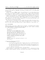
Example. This is a bad abstract:
Abstract In this paper, we discuss how to create a program that is useful for modeling
global warming. Unlike in the real world, however, where water vapor and carbon dioxide
both play an important role, our program makes simplifying assumption that there is only
one gas responsible for the greenhouse effect, whose concentration is proportional to reradiation of heat. Finally, results of simulations are presented.
Cut out deadwood and unnecessary elaboration, preserve the useful particulars, add some
specifics on the method and results, — and a much better version is obtained:
Abstract We discuss a computer simulation of global warming based on a simple mathematical model, in which one gas is responsible for the greenhouse effect and its concentration
is proportional to re-radiation of heat. The program iterates over time steps, one per season. Instability of temperature is observed if the intensity of gas emission exceeds a certain
critical value.
2.3.5
Introduction and Conclusion
If after glancing at the Abstract the readers feel the paper is not out of touch with their interests,
they browse through the Introduction and Conclusion. The central part of the paper, with all
the technicalities, is the last place the readers will go.
The Introduction, as the name suggests, should introduce the reader to the problem being
investigated. Motivation and historical background can be included (although some of it can
be scattered over later sections, too). The Introduction should also indicate what the reader
will find in the remainder of the report. The context and language of the Introduction often
Page 11
Chapter 2. Technical writing
2.3. Organization of report
makes it clear who the target audience is. Otherwise, state any special assumptions about the
readers’ background explicitly, e.g. “We assume the reader is familiar with eigenvalue theory
for matrices.”
When writing the Introduction, assume that the original assignment is not available to the
reader. Your paper must be self-contained. Do not copy the assignment’s language; use your
own words. Some assignments might introduce a little story and characters, like Alice and Bob.
In this case, again, your own Introduction must independently describe the situation — so that
the reader who didn’t see the assignment sheet would know what you are talking about.
The introduction can be viewed as an extended abstract, but it has a broader mission. Hook
the readers; make a promise that makes them want to stay with your paper. A potential reader
may never get to appreciate the rich and interesting contents if the introduction fails in its
mission.
For a typical paper in this course, the Introduction should be from 1/4 of a page to a full
page long. It should not tire the reader. It should be rather easy reading, not so technically
dense as the subsequent sections. In many cases it is not a place to put precise definitions,
but rather a place to motivate and anticipate them by describing the major concepts in a less
formal way.
Example 1.
The notion of two graphs having identical shape may be important. What exactly
does it mean for two graphs to have an identical shape? There are geometric definitions and analytic definitions. They will be discussed in Section 2.
Example 2.
When we say that one geometric figure is an expansion of another, there is an intuitive understanding of the two being alike and differing only in size. For the purposes
of this project, a precise geometric definition is required. It refers, in turn, to the
notion of isometry, or distance-preserving transformation of a plane, and to the
notion of homothety, which is stretching or squeezing in the same proportion along
all directions going from a fixed center. [Then the introduction proceeds informally. In
a later section, the technical definitions, say, in a coordinate form, are given.] ,
In some cases a precise technical definition properly belongs in the introduction. Suppose
the assignment asks you to write a program that counts in how many ways a given positive
integer N can be broken into a sum of positive integers. It is rather pointless in this case to
keep an informal tone. Get straight to the point:
The purpose of this laboratory is to design a method and to write a computer
program for counting partitions of integers.
Definition. A partition of a positive integer N is a set of positive integers arranged
in non-increasing order n1 ≥ n2 ≥ . . . ≥ nk such that n1 + n2 + . . . + nk = N .
Page 12
Chapter 2. Technical writing
2.3. Organization of report
You can help the reader to understand the definition without breaking away from the formal
style by adding a comment or remark explaining important particular cases. For example:
“A partition with the least value k = 1 consists of one element n1 = N . A partition with
maximum number of elements k = N is n1 = n2 = . . . = nN = 1”. The project may later deal
with special classes of partitions, say, those with non-equal members. It is not necessary (and
hardly appropriate) to put all definitions in the Introduction.
The last section — Conclusion, or Concluding Remarks — contains a brief summary of the
findings of your report. By reading only the summary, a reader should be able to ascertain the
most important facts resulting from your work. Do not overload the conclusion with details of
the results.
It is tempting to create the Conclusion from the Introduction by a simple “copy and paste”
method. However such an approach misses the point. Observe the difference. If your introduction sets up a goal or makes a promise (as we suggest it should), the conclusion serves as a
“checklist”: has the goal been reached? is the promise fulfilled? Sometimes the answer will be
— not quite; in that case, you should admit it and explain.
Example.
In this paper, a method for counting all partitions of a given positive integer N is
described. A FORTRAN program has been written and the number of partitions
has been computed for all N ≤ 30. It is apparent that the number of partitions
P (N ) exhibits a rather rapid growth as N increases. We observed and proved that
P (N ) > N 2 for N > 9 and that P (N ) < 2N for all N , but we did not come up with
a definite conclusion about the precise law describing the growth.
The program presented here uses direct enumeration of partitions. A Wikipedia
article [2] suggests another, supposedly more economical method for counting partitions, based on recurrence relations. We have also attempted to implement that
method but have not been able to complete the programming in a timely manner.
It is too late in the conclusion to bring in new material not found earlier in the paper.
Instead, you may discuss possible extensions of the work done or point out some connections
between your subject and other applications or techniques, which you might have come across
in the course of the work but which have not been been worked out in detail in the paper body.
The Introduction and Conclusion may contain other material that the author considers
relevant, for example, a personal remark or opinion which cannot be conveniently expressed in
the central, more formal part of the paper.
The size of the Conclusion should not exceed 1/2 of a page; in many cases, one or two
paragraphs will suffice. Avoid trivial, non-informative phrases, like “Upon completion of this
laboratory, certain conclusions can be drawn”. An Introduction or Conclusion longer than one
of the central sections is a sign that the material should be re-balanced.
Page 13
Chapter 2. Technical writing
2.3.6
2.3. Organization of report
Technical details
Other commonly used titles are “Method” or “Methodology”. Feel free to devise a subjectspecific, explanatory title. If the original problem has several parts, subdivide this section
accordingly. A subdivision may be needed simply for a better balance of section sizes or it can
be demanded by the logic of exposition: if, say, different aspects of the method employ different
techniques.
This section should describe all the fine (or heavy) details of the problem or model and the
details of the mathematical method or algorithm used to solve it, as well as the structure and
particulars of your computer code.
The requirements, in brief, are:
Attention to details and particulars. Relevance to the topic.
The subsection Mathematical details (or whatever your subject-specific title) generally
includes notation used, definitions, mathematical formulation (set-up) of a model, relevant
theoretical facts, and the mathematical essence of the algorithm used to solve the problem.
Do not attempt to reach far and wide; apply judgement. Suppose, for instance, that the
problem is to find the distance between two skew lines in space. A student googles for distance,
finds a Wiki article on metric spaces and blindly copies a definition to her paper. Big math, the
prof must be pleased!? — Wrong! Irrelevant! (Plus, the level is inappropriate for the target
audience, which is not the “prof”.)
Another student, faced with the equation x2 − 5x + 6 = 0, engages in a lengthy step by
step calculation using the quadratic formula. Five lines down, he finds the roots to be 2 and
3. It isn’t such a serious crime, but it wastes space on a triviality. In such simple cases, the
answer ought to be given next to the equation. (In more involved cases, a detailed solution of
a quadratic equation would make sense. Your reader may not immediately see that the roots
of the equation x2 − 2tx + (t2 − 1) = 0 are x1 = t + 1 and x2 = t − 1.)
Neither speculating about things you don’t understand nor reiterating banalities is good.
Focus on a content that’s not over your head and that really matters. Any symbol that appears
in your calculations, arguments, or later in tables and graphs, should be defined. Definitions
and terminology should be accommodated to the concrete situation. In an anecdotal case, a
student writing a paper on graphs of polynomial functions started with a definition of a graph
from Graph Theory!
Let us elaborate on definitions a bit further. They can be stated in two ways.
(1) As stand-alone structure units, in a separate paragraph, with the title word Definition in
a distinguished font style. This format should be used when you introduce a major concept or
when a definition is lengthy. (Do not hesitate to make definitions lengthy and detailed, even
boring: precision and disambiguation are the priorities. Think of a legal code.)
(2) Inline definitions (as a part of the flow) can be used if the definition is very short, simple
or natural, or if the concept is supposed to be generally familiar to the reader. Example: “To
describe the shape of a rectangle with side lengths a and b, we introduce the parameter µ = b/a
called the aspect ratio.”
Page 14
Chapter 2. Technical writing
2.3. Organization of report
The definitions, the notation, and the method should be described in such detail that a
motivated reader could reproduce your work on his/her own and obtain identical results.
How about yourself a few months later? Keep adding details and clarifying your writing until
you are able to answer in the affirmative. We refer to Appendix B-1, Section 4, for further tips
on mathematical writing. Let us just make one more suggestion regarding the mathematical
method in general and contents of your Mathematical details section in particular.
Think about simple particular cases, where the situation is either obvious or the answer
can be obtained easily. Do this before you write a program and before you explore the “real”
data, for which you cannot predict the results. While creating your program, you will have
convenient simple tests. For example, if you have to write a program to compute the area of a
triangle with sides 14.23, 12.497 and 9.72, test your program on the Pythagorean triangle with
sides 3, 4, 5 first; also test it in the case where a triangle degenerates to a segment (say, for the
sides 1, 2, and 3).
Also, think what happens when a certain parameter or a ratio of parameters becomes
extremely large or extremely small. Quite often, intuition will suggest an answer and you’ll be
in a better position to make sense of the computed results.
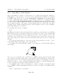
Example 1. Suppose, as a part of the assignment, you have to construct a common tangent
to two given circles. A circle collapses to a point when its radius tends to zero. Consequently,
a common tangent to the two given circles becomes a line passing through the two given points
when both radii shrink to zero. This limiting case provides a convenient test for your calculations
and your computer program.
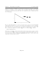
Example 2. Suppose the assignment asks you to find the number of grid points (whose both
coordinates are integers) inside the circle of radius R centered at the origin. Think what
happens as R → ∞. Every grid point corresponds to the unit square of which it is the center,
so the number of the grid points is approximately equal to the area of the circle, that is, πR2 .
The fraction of the area contributed by incomplete unit squares overlapping with the circle is
vanishingly small.
Considerations of this sort can make a valuable part of the Mathematical details section or
of the Results and Analysis section.
The subsection Program details should provide a detailed breakdown of your program so
that the reader can see how the mathematical ideas of the solution method are coded.
Please learn to differentiate between a mathematical method, or algorithm, and its programming implementation. Sometimes the description of the method and of the program,
which implements it, can be intertwined, especially if the method is very straightforward. In
other cases you are better to explain the method or its more subtle elements within Mathematical details, using conventional mathematical notation (dot or void for the multiplication sign,
one-letter variables, subscripted if needed, etc.). The explanation of a program involves the
actual syntax of the programming language used, with its own conventions (∗ for multiplication, multi-letter names of variables, etc.). If necessary, explain the correspondence between
mathematical variables and their counterparts in the program.
Page 15
Chapter 2. Technical writing
2.3. Organization of report
What is the best way to explain a computer program? On the one hand, from the end-user
perspective the program is a black box that takes a specified input and produces an output,
which the user should be in position to interpret. On the other hand, you must explain the
internals, the workings of the code, and — primarily — the part pertaining to mathematical
operations. It is the latter that we want you to emphasize in this section. You are writing a
research report, not a user manual (a technical text, too, but of a different kind).
If your program validates initial data (reports an error on input of a negative distance,
say) — good, but do not get overexcited about the user interface. It is better to make an
effort to explain the overall logic of the program, flow control (loops, if/else operators), and the
organization of data unless it is very obvious.
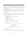
Example 1. Suppose your program counts the number of partitions P (N ) for N from 1 to 30.
Your description of the program can begin as follows:
Each run of the outermost loop of the program corresponds to computation of P (N )
for a particular value of N :
DO N=1,MAXN
Computation of P (N )
END DO
The upper bound, MAXN, of the loop is set to 30 by default, but it can be changed
through user’s input.
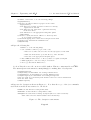
Example 2. A line like this
DISTANCE=TIME*SPEED
is self-explanatory and doesn’t need comments. A loop like this
DO I=TMIN+1,TMAX
DISTANCE=DISTANCE+DT*SPEED(I)
END DO
can be commented on at the author’s discretion, for example:
In this loop, the distance traveled over time interval from TMIN+1 to TMAX is computed. The array SPEED is initialized at the beginning of the program according
to formula (2.3). [referring to the Mathematical details section] The variable DT in the
program is time step, denoted by τ in the description of the method. Note that
the value SPEED(TMIN) is not included, since it has been included in the previous
summation.
The better your programming style, the easier it is to explain the program’s overall design
and logic. Look at Example 1 again. Perhaps, replacing the whole body of the loop (dozens
of lines of code) by a framed summary was a good writing trick. But it becomes altogether
unnecessary if a subroutine is used instead:
Page 16
Chapter 2. Technical writing
2.3. Organization of report
DO N=1,MAXN
CALL NUM_PARTITIONS(N)
END DO
Self-explanatory names of variables, short functions, transparent if/else conditions, avoiding
fancy syntax constructions like cond[--i]=(i>=1) in C, — all this helps.
Do not teach the reader the basics of programming. A general definition of a for loop copied
from the Internet or a general discussion of the organization of computer memory or a definition
of common data types (int, double) is not what is needed. If you really feel a need to remind
the readers about some syntaxic details or other particulars of the programming language used
— for instance, if you are writing for your own future reference — then, ok, find a place, but
don’t make it a big story. Even if you think (possibly correctly) that your instructor is not a
Java or Python guru, it is not a reason to incorporate a section-long language tutorial.
When it comes to small details, give priority to those that require special care. Why does
the value of J change from 0 to N-1 and not from 1 to N? Why is the variable numpoints defined
as double, while it naturally represents a positive integer quantity? (Conceivably, you want to
allow it to assume very large values, beyond the range of the type int.) Issues like these can
be addressed.
For the reader’s convenience, include only short, critical fragments of the actual code in the
body of the report. The complete listing can be included as an Appendix. In any case, the
program code must be submitted electronically as a part of the assignment bundle.
The above is not dogma. For example, it can be important to explain to the reader how
exactly your FORTRAN program produces the data file with coordinates — in which case the
details of the WRITE operator should be discussed, although it is not a computational issue.
2.3.7
Results and Analysis
As in the case with the Technical details section, this one can be subdivided if the research has
several parts.
In different projects, the meaning of “solution” or “results” is different. There have been
few labs in this course where the answer can be stated in a really short form, like projects asking
to decipher a coded message. In most labs, results come from a series of runs of a program that
a student creates. Each single outcome can be just a number or it can be an array of numbers,
a table or a graph.
As a bare minimum, your presentation of results should include:
• evidence that your mathematical method and your program are correct. Run sample cases
that can be checked by hand calculation. Or demonstrate the workings of your program
in cases where the solution is intuitively obvious.
• the solution(s) corresponding to those data provided in the assignment (if such data are
indeed provided).
Page 17
Chapter 2. Technical writing
2.3. Organization of report
If correctness of the method/program cannot be demonstrated because the program doesn’t
work correctly, read Sect. 1.3.2.
Many projects in this course are to some degree open-ended. They ask you to go beyond the
prescribed sets of data and to explore the problem further on your own. The assignment sheet
may or may not give a hint on how to choose data for such experimentation. Some outcomes of
your experiments will end up in a trash bin and some will make it into the paper. In the end,
we want your Results to be more than just plural for a single ‘result’. Interpret them, present
them as a manifestation of a certain idea or phenomenon. We want you to spot a trend, to
observe a pattern, to discover some sort of “law.”
• Tell the reader why or how each example presented is relevant to the conjectured “law.”
• Explain the observed pattern/law, at least partially.
The quality of your analysis of results and your mathematical explanations determine the
research value of your paper more than anything else. Remember that this is a mathematics course and a large component of your grade will be based upon the paper’s mathematical
content. Don’t just state observations. Analyse them and justify them! If the analysis and/or
explanation of the results requires a piece of theory that has not been discussed in the Mathematical details section, include the necessary definitions and facts here, along with your own
calculations and arguments.
In this section you can also explore the efficiency of your code: how fast or slow it is as the
size of data fed to the program increases.
2.3.8
Acknowledgements and References
Any help that you have received from another person must be acknowledged. An acknowledgement should be expressed in the form of a grammatically complete sentence. If possible, specify
the kind of help obtained. It also helps to characterize the status of the person so that those
who come across your paper in a few years will know. Don’t just say:
• John Smith for his help with this assignment.
Say instead:
John Smith, a Computer Science major, has provided advice about the input/output
functions in Java.
Or:
I acknowledge help from Mr. John Smith, a tutor, in justifying the pattern as
described in the Results section.
Page 18
Chapter 2. Technical writing
2.3. Organization of report
If you quote any printed material in your report, for example a calculus book, it must be
listed as a reference. You should provide specific page number to enable the reader to easily
find the place (definition, theorem, historical fact) you are referring to.
Example. In the body of the paper, put the reference number and the page number:
If we substitute the elliptic arc equation (2) into the arc length formula [3, p. 548]
Z bp
L=
1 + [f 0 (x)]2 dx,
a
we obtain the expression . . .
In the References section, describe the source:
[3] J. Stewart, Calculus: Early Transcendentals, 5th ed., Thomson-Brook/Cole, 2003.
(In this case, the publisher is a worldwide company and the place of publication is not indicated.)
There are different reference styles. Follow one style consistently. Check with your instructor
as to whether a particular style is preferred.
Quoted online resources must also be given proper attribution. For instance, there is a
webpage at http://mathworld.wolfram.com/ContinuityPrinciple.html. It has a title and,
unlike, say, many pages in Wikipedia, it is not anonymous: we can name an author. For this
particular page, a bibliographic entry would look like this:
[1] Eric W. Weisstein, Continuity Principle, http://mathworld.wolfram.com/
ContinuityPrinciple.html. (Accessed Dec. 5, 2008).
Alternatively, “web sites may be cited in running text instead of in an in-text citation” (The
Chicago Manual of Style Online, section Website). This very line is an example.
The sections Acknowledgments and References, as well as Abstract, are not numbered.
See Sect. 3.2 regarding LATEX typesetting conventions for these sections.
2.3.9
Appendix
Material that does not naturally fit in the flow of your paper yet is important for your project’s
completeness should be put in an Appendix. Many papers will not have an appendix. Where
an appendix is present, the following kinds of material are found in it:
• Computer code
• Graphs and illustrations
• Particularly long mathematical calculations or proofs
Page 19
Chapter 2. Technical writing
2.4. Suggestions about style
A listing of your program is the most common thing to put in the Appendix. Sect. 3.1.9
suggests how to get a nice printout.
A Math-2130 paper having more than one appendix should be an exception, but if that
happens, identify the appendices alphabetically: Appendix A, Appendix B.
We urge you to learn quickly how to include graphs and illustrations in the body of your
report. You may use gnuplot, xfig, the LATEX picture environment, Maple, or PostScript.
Graphs and illustrations which are not part of the text can comprise Appendix A of your report,
while the computer programs can be presented in Appendix B.
2.4
Suggestions about style
2.4.1
A note on spelling
There are many spelling checkers available. Use them! On Linux, you can use ispell. The
Kile editor has a built-in spell function which uses the ispell program. There is no excuse
for spelling errors, and they will be penalized heavily. However, be warned, the spell checker
will not find every error in spelling, nor can it pass judgement on a sentence like
A program too gene rate asset off inter resting numb hers ...
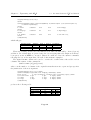
Some common spelling errors
• their (whose?) — there (where?)
• its (whose?) — it’s (it is)
• sep a rate (not sep e rate)
• occur e nce (not occur a nce)
• one’s — once
• two — to — too
• then (if ..., then) — than (more than)
• lab o ratory (not labratory)
2.4.2
Squeeze water out (Eliminate unnecessary words)
Compare:
(1) It can be shown by the implementation of the Cosine theorem that the distance AB is equal
to 5.
(2) Applying the Cosine theorem we see that AB = 5.
Page 20
Chapter 2. Technical writing
2.4.3
2.4. Suggestions about style
A note on “strong words”
Students often write: “it is necessary”, “one must” etc. Such strong expressions may justly
raise objections.
Example. Suppose we are considering the equation x2 − 6x + 5 = 0.
Bad description: “It is necessary to use the Quadratic Formula. Thus we obtain...”
Is it necessary? Absolutely not. Any one competent in quadratic equations will factor this one
on the spot. If you want to emphasize the method, better say:
√
“The roots, as given by the Quadratic Formula, are 12 (6 ± D), where D = 62 − 4 × 5 = 16.
Thus x1 = (6 + 4)/2 = 5, x2 = (6 − 4)/2 = 1. ”
Better even (if the method is of no special importance) is just to say
“The roots are x1 = 5 and x2 = 1”.
Of course, the style and level of details that you should or should not provide depend on who
your readers are. In any case, saying that to use the Quadratic Formula is necessary here is
unprofessional.
2.4.4
Common words in mathematical writing
Learn to use basic mathematical terminology precisely and avoid common misuses. For example,
watch the following as you write.
• An equation must have two parts (sides) connected by the = sign. A thing like
sin2 x + cos2 x is not an equation; it can be described as an expression or, more precisely,
√
as a trigonometric polynomial. Also don’t call x + y ≥ 2 xy an equation; it is an inequality.
• At the beginning of a mathematical argument you often make an assumption, while at
the end you arrive at a conclusion. Expressions like Assume (suppose) that something is ... or,
equivalently, Let something be are very standard. Steps of your argument or formulas that you
display or refer to should be verbally connected using words like imply, follow, yield, etc. to
make the flow of the argument smooth and its logic transparent.
• Here are some common, frequently used, safe verb-noun collocations.
— An equation can be solved (or solved for x). In contrast, a polynomial (like x2 − 5x + 6,
without any right-hand sign) cannot be solved (there is no equation to solve) but it may have
roots. Also, a polynomial can be evaluated at a particular point; equivalently, a particular
substitution can be made into it.
— A computer program can implement a method or an algorithm; it is created or written by
you; to obtain (produce) results you run (or execute) it; the results are presented or displayed
in tables and graphs.
— A value can be assigned to a variable (or a variable can be assigned a value). Also, a value
can be given √
in a closed form (as a mathematical expression that does not involve an approxi√
mation, e.g. 2 or arctan π/3) or approximately (as a decimal fraction), e.g. 1.414 for 2.
Page 21
Chapter 2. Technical writing
2.4. Suggestions about style
— An expression (a sum, an integral, but not an equation) can be evaluated (calculated, computed); also it can be transformed (into an equivalent form), expanded, factored, simplified,
reduced to a simpler form in a special (particular) case, broken into two or more parts (usually,
to reveal an essential structure). But do not “solve a sum”!
— A new concept or notation can be introduced, defined, or described in a manner of this sort:
let us say that X is . . . [an explanation in terms of known or previously defined terms follows].
2.4.5
We versus I
Whether you should write in the 1st person (we or I) or in the 3rd person is to a large extent
a matter of choice and personal style. It is more common to use I in the Introduction and
Conclusion only, if at all. If you are bold enough to use I in the main part of your paper, do so
consistently; do not hide behind we in “inconvenient” places.
That said, modern professional scientific writing overwhelmingly prefers we. Think about it
this way: as a reader goes through your paper, he/she feels your company and gentle support:
“We = I, the author, + you, the reader”.
You should use I when expressing personal opinions, e.g. “I found the results obtained in
this laboratory truly surprising.” There are other situations where the subject I sounds more
appropriate than we. Consider this example: “I have encountered difficulty implementing this
algorithm.” Substituting we in place of I would imply that your innocent reader shares your
responsibility for the trouble. Do not switch lightly between we and I. If the subject I is
indeed necessary, its use should be confined to a particular section — better the Introduction
or Conclusion — and there I, not we, should be used throughout.
While working on the project, you perform concrete actions, like searching a database,
writing a program, etc. If you feel uncomfortable to write we when describing such actions, use
sentences stated in the 3rd person. For example, “A program has been written” instead of “I
have written a program”. However, papers written in the 3rd person from the beginning to end
usually leave an impression of an indirect, cumbersome style.
2.4.6
Verb forms: tense, mood, modal verbs
Use present tense predominantly when discussing mathematical theories and other abstract
facts: they last indefinitely. Naturally, in talking about background and history of the problem
you would use the past tense.
You may choose to use either past or present to describe how you have created a computer
program and produced the results of numerical simulation. (The story may be the past for you
when you submit the report, but it will be current for the reader as he/she reads it.)
Variation of tense can be employed just for a particular purpose. Do not constantly swing
between one tense and another, especially within a paragraph or even a section.
Write in the indicative mood for the most part; use conditional only when it is unavoidable. Theorems are true, not would be true.
Page 22
Chapter 2. Technical writing
2.4. Suggestions about style
Watch other modal verbs, besides would. In many of students’ papers the verbs can and
must are unnecessarily frequent.
Example 1. Saying that “Equation (1) can be shown to yield formula (2)” leaves the reader
wonder whether you omit significant steps. If the answer is yes, you ought to show how the former yields the latter. Otherwise (if the connection between (1) and (2) is transparent enough),
simply say “Equation (1) yields formula (2).”
Example 2. Here must is used unnecessarily: “Therefore Equation (3) must hold when t = 0.”
It really means that “Equation (3) holds when t = 0.” Say thus — shorter and better.
Page 23
Chapter 3
Typesetting with LATEX
3.1
3.1.1
Elements of LATEX
Preamble
Every LATEX file has a structure like this:
\documentclass[12pt]{article}
\usepackage{2130}
.........
\begin{document}
.........
\end{document}
The part of the file before the line \begin{document} is called preamble, while the subsequent
part is called body of the document.
The first line in the file tells LATEX to use a file called article.sty as the main source of
formatting commands. The style file contains certain default parameters that determine layout
of the document, in particular:
\textwidth
\textheight
\topmargin
\oddsidemargin
\evensidemargin
The subsidiary style indicated by the argument “[12pt]” sets up the regular font size for the
document to be 12pt. Line spacing and sizes of fonts described in relative terms (Large, large,
small, tiny) thus become determined.
The first line may be followed by lines that import additional commands from various
packages. The package 2130.sty, which the second line in our document refers to, makes it
c MMIX Department of Mathematics and Statistics, Memorial University of Newfoundland
°
September 4, 2009
Chapter 3. Typesetting with LATEX
3.1. Elements of LATEX
easy to format a report for this course. For example, it will default to one inch margins all
around the standard size of paper. It also makes it easy to create the title page, headers and
footers, using the commands
\headers{...}{...}{...}
\underhead
\nounderhead
\underheadoverfoot
\footers{...}{...}{...}
\overfoot
\nooverfoot
The package 2130.sty also contains enhanced graphics command, which significantly extend a
graphical facility provided by the standard LATEX, as described in Section 4.4.3.
Other useful packages that you will likely need to include in your documents are graphicx
(to enable import of EPS graphics, see Section 4.3.1) and amssymb (to enable mathematical
symbols like R and various special characters, like ∅).
Besides \usepackage command(s), the preamble may contain your own definitions. For
example, this is a convenient shorthand for an useful but long LATEX’s keyword (see p. 28):
\newcommand{\ds}{\displaystyle}
User-defined commands may have parameters, for example: \newcommand{\pair}[2]{(#1,#2)}.
Now, the command \pair{A12}{b34} produces: (A12,b34).
3.1.2
Comments
The percent sign % is the commentary symbol in LATEX. Everything that follows it is ignored
till the end of line. There are two exceptions. First, the percent sign itself can be printed with
command \% and, as a part of this command, it does not begin a commentary. Second, the
percent sign within the verbatim environment or \verb command has no controlling effect.
If there is a need to disable rather long parts of a document from processing, while deleting
them is undesirable, the following construction can be used:
\iffalse
No matter how many lines or pages - everything here will be ignored by LaTeX
\fi
Finally, you may put the line \end{document} earlier in your document and LATEX will stop
exactly there. Everything that follows will be ignored. This is a convenient method to find and
fix errors in long documents.
3.1.3
Environments
The following construction, very common in LATEX, is called an environment:
\begin{something}
..........
\end{something}
Page 25
Chapter 3. Typesetting with LATEX
3.1. Elements of LATEX
In this case, we deal with a (nonexistent) “something”-environment. The whole document is
an environment by itself.
Some common environments are: displaymath, equation, tabular, picture, table, figure,
center, thebibliography, itemize, enumerate, verbatim.
3.1.4
Space
LATEX regards one ‘return’ or ‘enter’, one or more ‘tabs’ and one or more blank spaces, as
equivalent to one ‘space’. An exception to this rule is presented by the spaces within the \verb
command and the verbatim environment.
Paragraphs
There are two ways to start a new paragraph:
1. The usual (simplest) way is to leave a blank line in your text.
2. Use the command \par.
Line breaks
You may force LATEX to start a new line within the current paragraph by means of the command
\\ (double backslash). The current line ends immediately, at the same position as if the
paragraph had ended. The command \\ is routinely used as a separator between lines in tables
and “arrays” (multi-line formulas in math mode).
Another seemingly similar command is \linebreak. However it is rarely used. It causes
LATEX to stretch the current line to page width to compensate for the text that has been forced
out to the next line. LATEX may find the required stretch intolerable and deny the requested
line break.
Vertical space
LATEX does a reasonable job of inserting space and turning up new pages. Still, there are times
when the user would like to assert his/her own influence.
The regular, preferred method to add vertical space between paragraphs or figures is by
using one of the three commands:
\smallskip adds a little extra space to the regular space between lines
\medskip adds about twice that much
\bigskip adds yet about twice that much as \medskip.
Page 26
Chapter 3. Typesetting with LATEX
3.1. Elements of LATEX
The command \vspace{1ex} instructs LATEX to push the next line down by the height of
a letter “x” in the current font size. These commands ought to be given after a blank line (in
particular, they should not be given within a paragraph), otherwise the layout of your page
may turn out to be rather odd. The command \vskip 1ex has the same effect in most cases;
however, its use in LATEX documents is now deprecated.
There are several allowed measures of length, including inches (in), centimeters (cm) and
millimeters (mm), and finally, points (pt), which are the preferred unit to a typesetter. (There
are 72 points to an inch.) Besides these absolute units, the units relative to the current font size
are often used: \ex (see above) and \em (see below).
The command \vspace{...} has no effect at the top of a page or at the bottom. Why
would you want space when you are about to move to a new page? If you insist, you must use
\vspace*{...} to force LATEX to make space.
In the line break command inside a paragraph of text, as well as inside tables, arrays (in
math mode), and parboxes, one can create space by affixing an argument to the command \\;
for example, \\[1ex] leaves 1ex of additional space after the current line.
To make LATEX to skip more space between paragraphs, as is done throughout this Manual,
you may add the following command in the preamble of your document:
\setlength{\parskip}{\smallskipamount}
Finally, the commands \pagebreak and \newpage end the current page and start putting
text on the new one.
Horizontal space
The command \hspace{10pt} skips 10 points (approx. 3.5 mm) of horizontal space. (The
command \hskip 10pt has the same effect in most cases, but its use is discouraged.)
At the beginning of a line \hspace{..} will have no effect, so you must use the command
\hspace*{..} instead.
It is recommended that you use the units ‘em’ (the width of a letter ‘m’ in the current font
size) for horizontal space.
By default, paragraphs in LATEX begin with indentation, except those immediately after
the headings made with commands like \section. To suppress indentation, you can use the
command \noindent.
Math space
Spacing commands like \hspace and \vspace only work in “paragraph mode” (outside math).
The horizontal spacing commands in math mode are: \; \: \, \! \quad \qquad, which can
be found in Maltby.
That’s how much they measure: \,= | | and \:= | | and \;= | | and \quad= | | and \qquad
=|
|. The remaining distance \!= || is a tiny step backward!
Vertical spacing in math mode is best handled with \\[..].
Page 27
Chapter 3. Typesetting with LATEX
3.1. Elements of LATEX
Centering
To center a block of text, use the center environment:
\begin{center}
....
\end{center}
Note the American spelling of “center”. LATEX is very unforgiving if you make a spelling
error in a command.
3.1.5
Math mode
Inline math and displayed math
LATEX can typeset in a paragraph mode or in math mode, which, in its turn can be of two
kinds: inline math or displayed math. To begin and end the inline math mode, use the dollar
signs: $...$. This places the mathematical formula as the next word in the line of text, like
here: (x + y)(x − y) = x2 − y 2 . However, if you wish to display the formula, use
\begin{displaymath}
............
\end{displaymath}
A shorter delimiter for displayed math (both to begin and to end) is double dollar sign:
$$....$$.
The displayed formula is automatically centered on its own line. (This can be artificially
changed, but rarely needed.)
A displayed formula is still considered to be a part of a paragraph unless there is a blank
line separating it from the paragraph, before or after. In particular, the text following the
displayed math (without blank line in between) will not be indented.
A modification of the displaymath environment is the equation environment, which displays a single numbered equation, like this:
2 + 2 = 4.
(1)
LATEX automatically numbers equations enclosed in the equation environment consecutively
starting from (1). It does not number inline equations and equations within the displaymath
environment, but it does number equations within the eqnarray environment described below.
There is a difference in style of math formulas depending whether they are printed in the
inline or displayed math mode. In the displayed mode, for instance, fractions’ numerators and
denominators are printed in the regular font size, while in the inline mode they are printed in
a reduced font size. There is a way to force LATEX to type math in a prescribed mode: this
is done by the commands \displaystyle and \textstyle. There is also a similar command
\scriptstyle (to print in small size, like subscripts or superscripts).
Page 28
Chapter 3. Typesetting with LATEX
3.1.6
3.1. Elements of LATEX
Lists
Text (paragraph mode)
Use the ‘enumerate’ environment or the ‘itemize’ environment
\begin{enumerate}
\item ......
\item ......
.........
\item ......
\end{enumerate}
\begin{itemize}
\item ......
\item ......
.........
\item ......
\end{itemize}
to generate a numbered /bulletted list of items, respectively.
Math mode — \eqnarray
Here, we usually mean a set of equations. Use
\begin{eqnarray*}
<formula> & <connective> & <formula> \\
...
...
...
<formula> & <connective> & <formula> \\
\end{eqnarray*}
It is possible that some of the ‘< . . . >’ are empty fields. Also, the \\ can be replaced by \\[..]
as indicated in the section on vertical space above.
If the * is omitted, the equations will automatically be numbered. If a line is not to be
numbered, then the command \nonumber must be entered somewhere in that line.
Math — \array
The \array environment is used within displayed math in the cases when an additional flexibility as compared to \eqnarray is required. Details can be found in Maltby.
In both, \array and \eqnarray environments, LATEX is by default in the inline math
mode, so you have to use the \displaystyle command to display fractions, sums, etc. properly.
Moreover, this command only has effect between two ampersands or between an ampersand and
the endline command \\. So you may have to issue the \displaystyle command repeatedly.
That’s why the abbreviation shown on p. 25 makes a lot of sense.
Page 29
Chapter 3. Typesetting with LATEX
3.1.7
3.1. Elements of LATEX
Advanced math typesetting
The formula
xsin(x)
=
(cos(x))x
Z
∞
√
x
f (x) dx .
is obtained from
$$
\frac{x^{\sin(x)}}{(\cos(x))^x} \;=\; \int_{\sqrt{x}}^\infty\,f(x)\,dx\,.
$$
To the mathematically literate, many math commands are intuitive. If you want a symbol and
cannot remember it, try the obvious, and most times you will be correct!
You now should read Section 3.3, An Introduction to TEX and friends by Gavin Maltby. The
definitive book is the “LATEX User’s Guide and Reference Manual”, by Leslie Lamport.
3.1.8
Processing and viewing LATEX files
Every LATEX file must be saved with the .tex extension.1 You process the file “mylab.tex” with
the command
latex mylab
Note that there is no need for the extension .tex.
At this point, a lot of information will come across your screen. With time, much of it will
even make some sense. Everything you see on the screen, and more, gets written to a “log”
file. If you processed “mylab.tex”, LATEX will create “mylab.log” for you. If you are lucky and
have made no errors, LATEX will eventually stop and report that the output was written to
“mylab.dvi”. If you are less fortunate, LATEX will stop at the first error and leave you hanging
at a question mark on the screen. At this point, if you answer r (for run), LATEX will finish
processing to the best of its ability, writing all errors to “mylab.log” which one can then review
in one window while correcting “mylab.tex” in another.
To view “mylab.dvi”, you use a UNIX program called xdvi which is run like this:
xdvi mylab
Again, there is no need for the extension .dvi.
A .dvi can be converted to a .pdf file by the command like this:
dvipdf mylab
1
The description below has been in this Manual since its first edition and is still valid if you are working in
the UNIX command line. Many integrated environments like Kile, WinEdt, Texnic Center or Scientific Word
nowadays make processing a LaTeX document more comfortable.
Page 30
Chapter 3. Typesetting with LATEX
3.1.9
3.1. Elements of LATEX
Including source code in LATEX documents
There are a couple of ways in which you can include the source code from your programs in
your LATEX documents. One way is to use the verbatim environment:
\begin{verbatim}
Paste a copy of your code here
\end{verbatim}
Remember to break long lines by hand so that they fit the page width; otherwise some
details of your program will not be visible.
The other way to do so is to use lgrind, which formats program sources in a nice style.
Comments are placed in Roman font, keywords in bold face, variables in italics, and strings in
typewriter font. Source file line numbers appear in the right margin every 10 lines. Suppose
that you have a C program in the file sample.c. The first step towards including the file in the
document is to run it through lgrind to produce a file, say sample.tex:
lgrind -i -lc sample.c > sample.tex
This generates a file sample.tex, which has the pretty-printed version of sample.c with a lot of
LATEX commands. (Note that your program and main document should have different names!)
Now, in the declarations at the start of your main LATEX document file, you have to be sure to
include the lgrind package:
\usepackage{lgrind}
At the point in the document where you want to include the source code, give the command:
\lgrindfile{sample.tex}
Figure 3.1(A) presents an example of how the file would show in your document.
An alternative method of including source code, which does not require any intermediate
processing, would be to declare a few commands near the start of your LATEX document:
\newcommand{\beginverb}{\begin{verbatim}}
\newcommand{\inputfile}[1]{\input{#1}}
\newcommand{\verbatimfile}[1]{\expandafter\beginverb\inputfile{#1}}
and later on make use of the verbatimfile command:
{ \small
\verbatimfile{sample.c}
\end{verbatim} }
(Don’t forget to close the brace after \end{verbatim}; otherwise the rest of your document
will be printed in a small font size.)
The program listing printed with this method is displayed on Figure 3.1(B).
Page 31
Chapter 3. Typesetting with LATEX
A.
3.1. Elements of LATEX
/* This is a short C program to compute the sum of the integers
* from 1 to 1000 and print the result.
*/
#include <stdio.h>
#define N 1000
int Sum (int maxnum);
int main ()
{
printf ("The sum of the integers from 1 to %d is %d\n", N, Sum(N) );
return (0);
}
int Sum (int maxnum)
{
int i, total=0;
for (i=1 ; i<=maxnum ; i++)
total += i;
return (total);
}
B.
10
20
/* This is a short C program to compute the sum of the integers
* from 1 to 1000 and print the result.
*/
#include <stdio.h>
#define N 1000
int Sum (int maxnum);
int main ()
{
printf ("The sum of the integers from 1 to %d is %d\n", N, Sum(N) );
return (0);
}
int Sum (int maxnum)
{
int i;
int total=0;
for (i=1 ; i<= maxnum ; i++)
total += i;
return (total);
}
Figure 3.1: Source code printed (A) using \lgrind and (B) using \verbatimfile
Page 32
Chapter 3. Typesetting with LATEX
3.1.10
3.1. Elements of LATEX
Some commands defined in 2130.sty
Text commands
\TODAY produces dates in the form 22 December 2008.
\TODAYAT produces dates and time in the form 22 December 2008 at 14:57.
\Cents produces c|.
\INDENT forces an indented line when \indent fails.
\tildechar produces ~
\hatchar produces ^
\boxit{object} produces
object
\lbk, short for \linebreak, produces a line break with horizontal justification.
\pbk, short for \pagebreak, produces a page break with vertical justification.
\fsize{number} is an alternative way of changing font size. This was recommended by Lamport. \normalsize is \fsize{0}. Positive integers increase and negative integers decrease from
here.
For example \fsize{1} is equivalent to \large, and \fsize{-4} is equivalent to \tiny. Integers too large default to the smallest or largest fonts available.
Math commands
\di is short for \displaystyle
\toi produces → ∞
\dist produces dist
\slope produces slope
\LOngleftrightarrow produces ⇐==⇒ — compare
\Longleftrightarrow, which produces ⇐⇒.
\LOngleftarrow produces ⇐===
\LOngrightarrow produces ===⇒
\IFF produces <==> — compare \iff, which produces ⇐⇒
Page 33
Chapter 3. Typesetting with LATEX
3.2
3.2.1
3.2. Formatting your Math-2130 report in LATEX
Formatting your Math-2130 report in LATEX
Title page, footers and headers
A typical title page is shown on Figure 3.2. A LATEX code used to produce it is as follows.
\begin{titlepage}
\begin{center}
\large SHAPE MANIPULATION \\
AND MATRIX ALGEBRA
\end{center}
\vspace{6cm}
\hfill\begin{tabular}{ll}
AM 2130 & Lab 2 \\
Submitted by: & Unlikely Student \\
& \#200765432 \\
Submitted to: & Dr.~Good Professor \\
Feb. 18, 2009
\end{tabular}
\end{titlepage}
SHAPE MANIPULATION
AND MATRIX ALGEBRA
AM 2130
Submitted by:
Submitted to:
Feb. 18, 2009
Lab 2
Unlikely Student
#200765432
Dr. Good Professor
Figure 3.2: A sample title page for an AM2130 report.
Page 34
Chapter 3. Typesetting with LATEX
3.2. Formatting your Math-2130 report in LATEX
Your document will look nicer with running footers and headers. The following few lines
can be placed in the preamble or after the title page. The effect is explained in the comments.
\lhead{AM2130}
\rhead{Lab 1: Title}
\lfoot{Your Name}
\rfoot{\thepage}
\underheadoverfoot
3.2.2
%
%
%
%
%
appears in the header on the left
appears in the header on the right
appears in the footer on the left
page number, in the footer on the right
dividing lines: under header and below footer
Table of contents
Assuming you use the standard LATEX commands to structure your report (“section, “subsection), all that remains to produce the table of contents (TOC) is to insert the command
\tableofcontents
after the title page code.
You have to run LATEX compiler two times to obtain a correct TOC, as the first run just
creates an auxiliary file where the information about sections and subsections found is collected,
but LATEX is not able to incorporate that information into its dvi output immediately.
Some complication occurs with References and Appendix (assuming they are formatted as
suggested below). The command \thebibliography, which generates the list of references,
does not automatically yield an entry in TOC. You have to do some work by hand.
Somewhere soon after your \thebibliography command (perhaps, immediately after) insert the following line:
\addcontentsline{toc}{section}{References}
The heading References will then appear in your TOC and it will be printed in the same
style as section headers. If you want to somewhat de-emphasize References in TOC, modify
the above line:
\addcontentsline{toc}{subsection}{References}
Similarly, if you formatted your Appendix A using \section* command, you should put the
corresponding TOC line immediately after it, for example:
\addcontentsline{toc}{section}{Appendix A: Program source code}
3.2.3
Abstract
Abstract. The quote environment provides a nice format for an abstract. Type
the word Abstract in boldface and the rest in a regular font style. Abstract should
not be included in the TOC.
Page 35
Chapter 3. Typesetting with LATEX
3.2.4
3.2. Formatting your Math-2130 report in LATEX
The body of report
Use the \section{...} command for section headers, like Introduction, Technical Details, etc.
Use the \subsection{...} command for parts of the main sections.
Having third-tier headers (subsubsections) can hardly be justified in a typical Math-2130
report.
Acknowledgements and Appendix should not be numbered as regular sections. Use the
\section* command, for example,
section*{Acknowledgments}
The so formatted sections are not automatically referenced in the TOC. You should include a
reference to Appendix or Appendices, but probably not to Acknowledgements.
3.2.5
References
The list of references is printed using thebibliography environment. For example,
\begin{thebibliography}{4}
\bibitem{hagin} Frank G.~Hagin, A first course in differntial equations.
Prentice-Hall, Inc.:New Jersey. 1975.
%
\bibitem{m2130} Math-2130 Course Manual. MUN, 2008.
%
\bibitem{fourier-bio} ‘‘Jean Baptiste Joseph Fourier’’ (biography).\\
\verb+http://www-history.mcs.st-andrews.ac.uk/history/Mathematicians/+
\verb+Fourier.html+ \\ (Accessed December 2, 2008.)
%
\end{thebibliography}
Don’t forget to provide a numerical argument in \thebibliography line. It does not necessarily be equal to the actual number of references, it must just have the same decimal length
— like in our example, 3 references and the number is 4, both are single-digit numbers. In the
absence of the numerical argument LATEX often gives a misleading information as to where the
error is.
3.2.6
Appendix and program source
Use the \section* command for appendices. Section 3.1.9 explains how to include the source
code of your program in the report. (It is not always necessary.)
A little note for those who needs to include a Maple code in the report: in our experience,
the quickest way that does not compromise on typographical quality is simply to copy and paste
the lines from Maple worksheet into the LATEX file line by line. Maple programs (at least those
in Math-2130 projects) are usually rather compact. Maple’s numerical outputs can also be
Page 36
Chapter 3. Typesetting with LATEX
3.2. Formatting your Math-2130 report in LATEX
copied and pasted, unless they contain exponents. In the latter case please take a trouble to
type the answer properly in the LATEX math mode, for example, 6.67 × 10−11 . If there are too
many such numbers to type, think about summarizing them in a table rather than just copying.
Maple’s symbolic answers, when copied into a text file, are difficult to read. Again, if the
answer is important (so you are not just filling up a space), it is worth to neatly re-type in a
proper mathematical format. Important results can hardly be too many...
A copy of your Maple worksheet submitted electronically is a definitive document and will
be used by the instructor should any discrepancy between your reported input and Maple’s
output be revealed.
3.2.7
Floating environments: figures and tables
LATEX has its own ideas as to where it is best to place your figures and tables made by means
of the corresponding environments. In the processed document, it usually does not put them
where they ought to be according to their position in the source .tex file. Many students, and
not only, often find this frustrating.
However, LATEX’s behaviour is in most cases backed by well established rules and conventions
of typography. In general, try not to fight LATEX very hard. If it puts your figure on top of the
next page rather than dropping it just on spot, think whether you can agree with that decision.
Only if the displacement of the figure leads to a mess in the logic of your presentation or if a
large unfilled area remains on the page, you should insist.
The way to make LATEX to put the picture exactly here is to use the figure environment
with argument [H]:
\begin{figure}[H]
The option H is not provided by standard LATEX, you must \usepackage{float} in order to
be able to use it. All this equally applies to the table environment.
3.2.8
Automatic numbering, cross-references, and citations
The \caption command within a figure or table environment assigns a number to the figure
or table. This number can be captured by the \label command put right after. For example,
the command \label{xyz} allows you to refer to your figure elsewhere in your document in
the following way:
“See Figure~\ref{xyz} on page~\pageref{xyz}.”
Similarly, labels can be assigned to sections, subsections (Sect. 3.2.4), equations (Sect. 3.1.5)
and theorem-like environments described in Section 3.4.6.
References to sources listed under \thebibliography command can be done as follows:
Fourier’s memoir ‘‘On the Propagation of Heat in Solid Bodies’’ was
read to the Paris Institute on 21 December 1807 \cite{fourier-bio}.
Page 37
Chapter 3. Typesetting with LATEX
3.3
3.3. An introduction to TEX and friends
An introduction to TEX and friends
Original text by Gavin Maltby (1992); adapted by Math-2130 Instructors (1995,1998,2008)
3.3.1
An Introduction to TEX
TEX is well known to be the typesetting package, and a vast cult of TEX lovers has evolved.
But to the beginning TEX user, or to someone wondering if they should bother changing to
TEX, it is often not clear what all the fuss is about. After all, are not both WordPerfect and
Microsoft Word capable of high quality output? Newcomers have often already seen what TEX
is capable of (many books, journals, letters are now prepared with TEX) and so expect to find
a tremendously powerful and friendly package. In fact they do, but that fact is well hidden
in one’s initial TEX experiences. In this section we describe a little of what makes TEX great,
and why other packages cannot even begin to compete. Be warned that a little patience is
required—TEX’s virtues are rather subtle to begin with. But when the penny drops, you will
wonder how you ever put up with anything different.
TEX is a typesetter, not a word-processor
TEX was designed with no limiting application in mind. It was intended to be able to prepare
practically any document—from a single page all-text letter to a full blown book with huge
numbers of formulae, tables, figures etc.
Conventional word processors have a fundamental limitation in that they try to “keep up”
with you and “typeset” your document as you type. This means that they can only make
decisions at a local level (eg, it decides where to break a line just as you type the end of the
line). TEX’s secret is that it waits until you have typed the whole document before it typesets
a single thing! This means that TEX can make decisions of a global nature in order to optimise
the aesthetic appeal of your document. It has been taught what looks good and what looks
bad (having been given a measure of the “badness” of various possibilities) and makes choices
for your document that are designed to make it “minimally bad”.
But TEX’s virtues run much deeper than that, which is just as well because it is possible to
get satisfactory, though imperfect, results from some word processors. One of TEX’s strongest
points is its ability to typeset complicated formulae with ease. Not only does TEX make hundreds of special symbols easily accessible, it will lay them out for you in your formulae. It has
been taught all the spacing, size, font, . . . conventions that printers have decided look best in
typeset formulae. Although, of course, it does not understand any mathematics it knows the
grammar of mathematics—it recognises binary relations, binary operators, unary operators,
etc. and has been taught how these parts should be set. It is consequently rather difficult to
get an equation to look bad in TEX.
Another advantage of compiling a document after it is typed is that cross-referencing can
be done. You can label and refer back to chapters, sections, tables etc. by name rather than
Page 38
Chapter 3. Typesetting with LATEX
3.3. An introduction to TEX and friends
absolute number, and TEX will number and cross-reference these for you. Similarly, it will
compile a table of contents, glossary, index and bibliography for you.
Essential to the spirit of TEX is that it formats the document whilst you just take care of the
content, making for increased productivity. The cross-referencing just mentioned is just part
of this. Many more labour-saving mechanisms are provided for through class and style files.
These are generic descriptions of classes of documents, teaching TEX just how each class likes
to be formatted. This is taught in terms of font preferences, default page sizes, placement of
title, author, date, etc. For instance, a paper style file could teach TEX that when typesetting
a theorem it should embolden the part that states the theorem number and typeset the text
of the theorem statement in slanted Roman typeface (as in many journals). The typist simply
provides and indication that a theorem is being stated, and then types the text of the theorem
without bothering to choose any fonts or do any formatting—all that is done by the style file.
Style files exist for all manner of document—letters, articles, papers, books, proceedings, review
articles, and so on.
There are many other motivations one could cite for the superiority of TEX. But it is time
that we started to get our hands dirty. The novice reader will still have no idea of what a TEX
source file looks like. Indeed, why do we keep referring to it as a source file? The fact of the
matter is that TEX is essentially a programming language. Just as in any compiled language
(e.g., Fortran, C) one prepares a source file and submits it to the compiler which attempts to
produce an object file (.dvi file in the TEX case). To learn TEX is to learn the command syntax
of the commands that can be used in the source file.
Typical TEX interfaces
By the nature of TEX most time is spent editing the source document (before submitting it
for compilation). No special interface is necessary here, you just use your favourite text editor
(perhaps customising it to enhance TEXnical typing). Thus TEX user interfaces are usually
small and simple, often even missing. One frequently uses TEX at command line level, just
running the editor, compiler etc. as you need them. Sometimes a TEXshell program is present,
which runs these for you when you choose various menu options.
Whatever the interface, there are just a few basic steps to preparing a document:
1. Choose a document style to base your document on (e.g., letter, article).
2. Glance through the material you have to type, and decide what definitions might be
made to save you a lot of time. Also, decide on the overall structure of the prospective
document (e.g., will the largest sectional unit be a chapter or a part?). If you are going
to compose as you type, then pause a moment to think ahead and plan the structure of
your document. The importance of this step cannot be overstressed, for it makes clear in
your mind what you want from TEX.
3. Prepare your input file, specifying only the content and the logical structure (parts, sections, theorems,...) thereof and forgetting about formatting details.
4. Submit your input, or source, file to the TEX compiler for compilation of a .dvi file.
Page 39
Chapter 3. Typesetting with LATEX
3.3. An introduction to TEX and friends
5. If the compiler finds anything in your source file strongly objectionable, say incorrect
command syntax, then return to editing.
6. Run a previewer to preview your compiled document on the screen.
7. Go back to editing your document until glaring errors have been taken care of.
8. Make a printout of your compiled document, and check for those errors that you failed to
notice on the screen.
Performing these steps may be effected through typing at the system prompt (bare-bones technique) or through choosing menu options in a TEXshell program. The latter will probably
provide some conveniences to make your life easier.
3.3.2
A review of LATEX
The TEX typesetting system was designed by the eminent Stanford computer scientist Donald
Knuth, on commission from the American Mathematical Society. It was designed with enormous
care, to be ultimately powerful and maximally flexible. The enormous success of Knuth’s design
is apparent from the vast number of diverse applications TEX has found. In reading the following
you must keep one thing clearly in mind: there is only TEX language, and all the other packages
whose names end in the suffix -TEX simply harness its power via a whole lot of complicated
macro definitions.
TEX proper is a collection of around 300 so called primitive typesetting commands. These
work at the very lowest level, affording enormous power. But to make this raw power manageable, some macros must be defined to tame raw TEX somewhat.
In the few years after the initial TEX release (1982), the macro package LATEX was born.
LATEX was written for general usage. LATEX scores high points for its enhanced command syntax.
By far the majority of LATEX users will never have to learn “raw” TEX, for they will be shielded
from direct exposure by the numerous powerful macro packages.
Pre-amble
Every LATEX document begins with a pre-amble. This consists of a set of commands that tells
TEX how to process the document. We will explain the important parts of this in the next two
sections. The first (documentclass) is mandatory, whereas the others are all optional.
Document classes
We have explained the concept of a document class. It remains to name a few, and indicate
where they would be used. One always has to choose a document class when preparing a
document with LATEX.
The basic document classes in LATEX are article, letter, report, and book. Many more
are available, but these few cover the majority of straightforward applications. This is because
classes are not rigid—you can impose your own parameter choices if you want. So one chooses
Page 40
Chapter 3. Typesetting with LATEX
3.3. An introduction to TEX and friends
the class that most closely approximates the document you have in mind, and performs some
minor tweaks here and there. The article class is used for documents that are to have the
appearance of a journal or magazine article, and is the class that should be used for your reports
in this course. The report class is usually used for larger documents than the article class.
These classes really only differ in their choice of default page size, font, placement of title and
author, sectional units, etc. and on how they format certain LATEX constructs. You use the
same LATEX commands in each. Since the examples here will be small, we will choose to use
the article document class.
There are a number of possible options with each document class. The syntax for choosing
a document class follows. Do not worry if this leaves you with no idea of how to choose a
document style, for we will soon be seeing some examples. Also, remember that an argument
in square brackets is optional, and can omitted altogether (including the brackets).
\documentclass [options ]{class }
where class is the main document class (eg. report) and the optional argument options is a
list of document style options chosen from, for example, the following list:
11pt
chooses 11-point as the default font size for the document,
instead of the default 10-point.
12pt
chooses 12-point as the default font size.
twoside
formats output as left and right pages, as in a book.
twocolumn produces two-column magazine like output.
titlepage applies to the article style only, causing the title and
abstract to appear on a page each.
In fact there are many, many more document class options but we will not mention any
more here.
Packages
To modify further the main document class, we make use of style files. They are used as
in the following example:
\usepackage [options ]{package } where package is the
modifying style file and options is a list of style files modifying the style file.
For example, here is a possible preamble:
\documentclass{article}
\usepackage{amsmath}
\usepackage{2130}
3.3.3
Special symbols
In the coming sections we will see that the the ten characters
# $ % & ~ _ ^ \ { }
are reserved for special use.
Page 41
Chapter 3. Typesetting with LATEX
3.3. An introduction to TEX and friends
But what if we need one of these special symbols to appear in our document? The answer
for seven of the symbols is to precede them by a \ character, so forming another control symbol
(remember that \ followed by a space was also a control symbol) .
It is not 100\% straightforward to typeset the
characters \$ \& \% \_ \{ \}, but given the
enormous convenience of the use they are normally
reserved for this is a small price to pay.
produces
It is not 100% straightforward to typeset the characters $ & % { }, but given the
enormous convenience of the use they are normally reserved for this is a small price to pay.
So what are control symbols and words?
In typing a document, we can think of ourselves as being in one of two distinct modes. We are
either typing literal text (which will just be set into neat paragraphs for us) or we are typing
text that will be interpreted by LATEX as an instruction to insert a special symbol or to perform
some action. Thus we are either typing material that will go straight into the document (with
some beautification), or we are giving commands to LATEX.
Some commands are implicit, in that we do not have to do anything much extra. For
instance, we command LATEX to end the present sentence by typing a period (that does not
follow a capital letter). These are not so much commands as part of having to describe the
logical structure of a document.
A control word is something of the form \commandname, where the command name is a
word made up only of the letters a to z and A to Z. A control symbol consists of a \ followed
by single symbol that is not a letter.
Here are some examples:
• we have met the control space symbol \Ã before,
• the commands to set symbols like % and $ are control symbols
• \@ is a control symbol that told LATEX that the very next period did really end the
sentence,
• \LaTeX is a control word that tell LATEX to insert its own name at the current point,
• \pm instructs that a ± be inserted,
• \div inserts a ÷ symbol,
• \infty inserts a ∞ symbol,
• \em makes the ensuing text be emphasized.
Page 42
Chapter 3. Typesetting with LATEX
3.3. An introduction to TEX and friends
These examples show that control sequences can be used to access symbols not available
from the keyboard, do some typesetting tricks like setting the word LATEX the way it does, and
change the appearance of whole chunks of text as with \em. We will be meeting many more of
these type of control sequences.
Incidentally, underlining was the traditional way in which writers, working only with typewriters, were able to provide emphasis. Nowadays, underlining is poor form because it so easy to
italize. With TEX, use {\em something pretty long} or \emph{a word or two} to produce
something pretty long or a word or two.
Another enormously powerful class of control sequences is those that accept arguments.
They tell LATEX to take the parts of text you supply and do something with them—like make
a fraction by setting the first argument over the second and drawing a line of the appropriate
length between them. These are part of what makes LATEX so powerful, and here are some
examples.
• \overline{words} causes words to be overlined,
• \frac{a+b}{c+d} sets the given two argument as a fraction, doing most of the dirty work
for us: a+b
c+d ,
√
• \sqrt[5]{a+b} typesets the fifth-root of a + b, like this: 5 a + b. The 5 is in square
brackets instead of braces because it is an optional argument and could be ommited all
together (giving the default of square root),
Mandatory arguments are given enclosed by braces, and optional arguments enclosed by
square brackets. Each command knows how many arguments to expect, so you do not have to
provide any indication of that.
We have actually jumped the gun a little. The above examples include examples of mathematical typesetting, and we have not yet seen how to tell LATEX that it is typesetting math as
opposed to some other random string of symbols that it does not understand either. We will
come to mathematical typesetting in good time.
We need to dwell on a TEXnicality for a moment. How does LATEX know where the name
of a control sequence ends? Will it accept both \pm3 and \pm 3 in order to set ±3, and will
\emWalrus and \em Walrus both be acceptable in order to get Walrus? The answer is easy
when you remember that a control word consists only of alphabetic characters, and a control
symbol consists of exactly one nonalphabetic character.
So to determine which control sequence you typed, LATEX does the following:
1. when a \ character is encountered, LATEX knows that either a control symbol or a control
word will follow.
2. If the \ is followed by a nonalphabetic character, then LATEX knows that it is a control
symbol that you have typed. It then recognises which one it was, typesets it, and goes
on to read the character which follows the symbol you typed.
Page 43
Chapter 3. Typesetting with LATEX
3.3. An introduction to TEX and friends
3. If the \ is followed by an alphabetic character, then LATEX knows that it is a control word
that you have typed. But it has to work out where the name of the control word ends and
where the ensuing text takes over again. Since only alphabetic characters are allowed,
LATEX reads everything up to just before that first nonalphabetic character as the control
sequence name. Since it is common to delimit the end of a control word by a space, LATEX
will ignore any space that follows a control word, since you want that space treated as
end-of-control-word space rather than interword space.
This has one important consequence: The character in the input file immediately after a
control symbol will be “seen” by LATEX, but any space following a control word will be discarded
and never processed. This does not affect one much if you adopt the convention of always typing
a space after a control sequence name.
There is a rare circumstance in which this necessitates a little extra work and thought,
which we illustrate by example:
If we type a control word like \LaTeX in the running text
then we must be cautious, because the string of spaces that
come after it will be discarded by the \LaTeX\ system.
which produces the output
If we type a control word like LATEXin the running text then we must be cautious,
because the string of spaces that come after it will be discarded by the LATEX system.
Accents
LATEX provides accents for just about all occasions. They are accessed through a variety of
control symbols and single-letter control worlds which accept a single argument—the letter to
be accented. These control sequences are detailed in table 3.1.
\‘{o}
\’{o}
\^{o}
\"{o}
\~{o}
\={o}
\.{o}
ò
ó
ô
ö
õ
ō
ȯ
(grave accent)
(acute accent)
(circumflex or “hat”)
(umlaut or dieresis)
(tilde or “squiggle”)
(macron or “bar”)
(dot accent)
\u{o}
\v{o}
\H{o}
\t{oo}
\c{o}
\d{o}
\b{o}
ŏ
ǒ
ő
oÄ o
o̧
o.
o
¯
(breve accent)
(háček or “check”)
(long Hungarian umlaut)
(tie-after accent)
(cedilla accent)
(dot-under accent)
(bar-under accent)
Table 3.1: Control sequences for accents
Thus we can produce ó by typing \’{o}, ǎ by typing \v{a}, and Pál Erdös by typing
P\’{a}l Erd\"{o}s. Take special care when accenting an i or a j, for they should lose their
dots when accented. Use the control words \i and \j to produce dotless versions of these
letters. Thus the best way to type to type ĕxı̆gent is \u{e}x\u{\i}gent.
Page 44
Chapter 3. Typesetting with LATEX
3.3.4
3.3. An introduction to TEX and friends
Formatting
Font commands
We have seen a little of how to access various symbols using control sequences and we mentioned
the \em command to emphasize text, but we did not see how to use them. We look here at
commands that change the appearance of the text.
Each of the control words here is a directive rather than a control sequence that accepts an
argument. This is because potential arguments consisting of text that wants to be emboldened
or emphasized are very large, and it would be a nuisance to have to enclose such an argument
in argument-enclosing braces.
To delimit the area of text over which one of these commands has effect (its scope) we make
that text into what is called a group. Groups are used extensively in LATEX to keep effects local
to an area, rather than affecting the whole document. Apart from enhancing usability, this also
in a sense protects distinct parts of a document from each other.
The LATEX commands for changing type style are given in table 3.2, and those for changing
type size are given in table 3.3. Commands for selecting fonts other than these are not discussed
here.
\rm
\em
\bf
Roman
Emphasized
boldface
\it
\sl
\sf
italic
slanted
sans serif
\sc
\tt
Capitals
typewriter
Table 3.2: Commands for selecting type styles
Each of the type style selection commands selects the specified style but does not change
the size of font being used. The default type style is roman (you are reading a roman style
font now). To change type size you issue one of the type size changing commands in table 3.3,
which will select the indicated size in the currently active style.
size
\tiny
\scriptsize
\footnotesize
\small
\normalsize
\large
\Large
\LARGE
\huge
\Huge
default (10pt)
5pt
7pt
8pt
9pt
10pt
12pt
14pt
17pt
20pt
25pt
11pt option
6pt
8pt
9pt
10pt
11pt
12pt
14pt
17pt
20pt
25pt
12pt option
6pt
8pt
10pt
11pt
12pt
14pt
17pt
20pt
25pt
25pt
Table 3.3: LATEX size-changing commands.
Page 45
Chapter 3. Typesetting with LATEX
3.3. An introduction to TEX and friends
The point-size option referred to in table 3.3 is that specified in the \documentclass command issued at the beginning of the input file. Through it you select that base (or default) font
for your document to be 10, 11, or 12 point Roman. If no options are specified, the default is
10-point Roman. The table shows, for instance, that if I issue a \large in this document for
which I chose the 12pt document class option the result will be a 14-point Roman typeface.
We mentioned that to restrict the scope of a type-changing command we will set the text
to be affected off in a group. Let us look at an example of this.
When we want to {\em emphasize\/} some text we
use the {\tt em} command, and use grouping to
restrict the scope. We can change font {\large sizes}
in much the same way. We can also obtain {\it italicized},
{\bf emboldened}, {\sc Capitals} and {\sf sans serif} styles.
When we want to emphasize some text we use the em command, and use grouping to
restrict the scope. We can change font sizes in much the same way. We can also obtain
italicized, emboldened, Capitals and sans serif styles.
Notice how clever grouping allows us to do all that without once having to use \rm or
\normalsize.
One more thing slipped into that example—an italic correction \/. This is a very small
amount of additional space that we asked to be inserted to allow for the change from sloping
emphasized text to upright text, because the interword space has been made to look less substantial from the terminal sloping character. One has to keep an eye open for circumstances
where this is necessary. See the effect of omitting an italic correction after the emphasized text
earlier in this paragraph.
One might expect, by now, that LATEX would insert an italic correction for us. But there
are enough occasions when it is not wanted, and there is no good rule for LATEX to use to decide
just when to do it for us. So the italic correction is always left up to the typist.
Sentences and paragraphs
Let us create our very first LATEX document, which will consist of just a few paragraphs.
As mentioned above, paragraph input is free-form. You type the words and separate them
by spaces so that LATEX can distinguish between words. For these purposes, pressing Return is
equivalent to inserting a space—it does not indicate the end of a line, but the end of a word.
You tell LATEX that a sentence has ended by typing a period followed by a space. LATEX ignores
extra spaces; typing three or three thousand will get you no more space between the words
that these spaces separate than typing just one space. Finally, you tell LATEX that a paragraph
has ended by leaving one or more blank lines. In summary: LATEX concerns itself only with
the logical concepts end-of-word, end-of-sentence, and end-of-paragraph. Sounds complicated?
The example in Figure 3.3 should clear things up. Try running LATEX on this input.
We have learned more than just how LATEX recognises words, sentences and paragraphs.
We have also seen how to specify our choice of document class and how to tell LATEX where our
document begins and ends. Any material that is to be printed must lie somewhere between the
Page 46
Chapter 3. Typesetting with LATEX
3.3. An introduction to TEX and friends
\documentclass{article}
\begin{document}
Words within a sentence are ended by spaces. One space
between words is
equivalent
to any number. We are only
interested in separating
one
word
from
the
next, not in formatting
the space between them.
For these purposes, pressing Return
at the end of a line
and starting a new word on the next line
just serves to separate
words, not to cut a line short.
The end of a sentence is indicated by a period
followed by one or more spaces.
The end of a paragraph is indicated by leaving a blank line.
All this
means that we can type without too much regard for layout, and
the typesetter will sort things out for us.
\end{document}
produces the result
Words within a sentence are ended by spaces. One space between words is equivalent
to any number. We are only interested in separating one word from the next, not in
formatting the space between them. For these purposes, pressing Return at the end of a
line and starting a new word on the next line just serves to separate words, not to cut a
line short. The end of a sentence is indicated by a period followed by one or more spaces.
The end of a paragraph is indicated by leaving a blank line. All this means that we can
type without too much regard for layout, and the typesetter will sort things out for us.
Figure 3.3: Some TEX input and the corresponding output
declaration of \begin{document} and that of \end{document}. Definitions that are to apply
to the entire document can be made before the declaration of the document beginning. The
specification of document class must precede all other material.
In future examples we will not explicitly display the commands that select document class
and delimit the start and end of the document. But if you wish to try any of the examples,
do not forget to include those commands. The article document class will do for most of our
examples. Of course, the preceding example looks not at all like an article because it is so short
and because we specified no title or author information.
Most of what you need to know to type regular text is contained in the example above.
When you consider that by far the majority of any document consists of straight text, it is
obvious that LATEX makes this fabulously straightforward. LATEX will do all the routine work
of formatting, and we simply get on with the business of composing.
LATEX does more than simply choose pleasing line breaks and provide natural spacing when
setting a paragraph. Remember we said that TEX has inherited the knowledge of generations of
professional printers—well part of that knowledge includes being on the look-out for ligatures.
Page 47
Chapter 3. Typesetting with LATEX
3.3. An introduction to TEX and friends
These are combinations of letters within words which should be typeset as a single special
symbol because they will “clash” with each if this is not done. Have a look at these words
flight, flagstaff, chaff, fixation
and compare them with these
flight, flagstaff, chaff, fixation
See the difference? In the first set I let LATEX run as it usually does. In the second I overruled it
somewhat, and stopped it from creating ligatures. Notice how the ‘fl’, ‘ff’, and ‘fi’ combinations
are different in the two sets—in the former they form a single symbol (a ligature) and in the
latter they are comprised of two disjoint symbols. There are other combinations that yield
ligatures, but we do not have to bother remembering any of them because LATEX will take care
of these, too.
Notice, too, that LATEX has been taught how to hyphenate the majority of words. It will
hyphenate a word if it feels that the overall quality of the paragraph will be improved. For long
words it has been taught several potential hyphenation positions.
LATEX also goes to a lot of trouble to try to choose pleasing page breaks. It avoids “widows”,
which are single lines of a paragraph occurring by themselves at either the bottom of a page
(where it would have to be the first line of a paragraph) or at the top of a page (where it would
have to be the last). It also “vertically justifies” your page so that all pages have exactly the
same height, no matter what appears on them. As testimony to the success of the pagebreaking
algorithm, I have (to this point) not once chosen a page break in this document.
Punctuation
Typists have a convention whereby a single space is left after a mid-sentence comma, and two
spaces are left after a sentence-ending period. How do we enforce this if LATEX treats a string
of spaces just like a single one? The answer, unsurprisingly, is that we do not.
To have a comma followed by the appropriate space, we simply
type a comma follows by at least one space. To end a sentence
we type a period with at least one following space.
No space will
be inserted if we type a comma or period followed straight away
by something other than a space, because there are times when
we will not require any space, i.e., we do what comes naturally.
will produce
To have a comma followed by the appropriate space, we simply type a comma follows
by at least one space. To end a sentence we type a period with at least one following
space. No space will be inserted if we type a comma or period followed straight away by
something other than a space, because there are times when we will not require any space,
i.e., we do what comes naturally.
LATEX will produce suitable space after commas, periods, semi-colons and colons, exclamation marks, question marks etc. if they are followed by a space. In stretching a line to
justify to the right margin, it also knows that space after a punctuation character should be
Page 48
Chapter 3. Typesetting with LATEX
3.3. An introduction to TEX and friends
more “stretchable” than normal inter-word space and that space after a sentence-ending period
should be stretched more than space after a mid-sentence comma. TEX knows the nature of
punctuation if you stick to the simple rules outlined here. As we have already said, those rules
tell LATEX how to distinguish consecutive words, sentences, phrases, etc.
Actually, there is more to ending sentences than mentioned above. Since LATEX cannot speak
English, it works on the assumption that a period followed by a space ends a sentence unless
the period follows a capital letter. This works most of the time, but can fail. To get a normal
inter-word space after a period that does not end a sentence, follow the period by a control
space—a \Ã (a \ character followed by a space or return). Very rarely, you will have to force a
sentence to end after a period that follows a capital letter (remember that LATEX assumes this
does not end a sentence). This is done by preceding the period with a \@ command (you can
guess from the odd syntax that this is rarely needed).
It is time we saw some examples of this. After all, this is our first experience of control
symbols (do not worry, there are many more to come).
We must be careful not to confuse intra-sentence periods
with periods that end a sentence, i.e.\ we must remember
that our task is to describe the sentence structure. Periods
that the typesetter requires a little help with typically result
from abbreviations, as in etc.\ and others. We have to work
somewhat harder to break a sentence after a capital letter,
but that should not bother us to much if we keep up our intake
of vitamin E\@. All this goes for other sentence-ending
punctuation characters, so I could have said vitamin E\@!
Fortunately, these are rare occurrences.
results in
We must be careful not to confuse intra-sentence periods with periods that end a
sentence, i.e. we must remember that our task is to describe the sentence structure. Periods
that the typesetter requires a little help with typically result from abbreviations, as in etc.
and others. We have to work somewhat harder to break a sentence after a capital letter,
but that should not bother us to much if we keep up our intake of vitamin E. All this
goes for other sentence-ending punctuation characters, so I could have said vitamin E!
Fortunately, these are rare occurrences.
Quotation marks is another area where LATEX will do some work for us. Keyboards have
the characters ‘, ’, and " but we want to have access to each of ‘, ’, “, and ”. So we proceed
like this:
‘\LaTeX’ is no conventional word-processor, and
to to get quotes, like ‘‘this’’, we type repeated
{\tt ‘} and {\tt ’} characters. Note that modern
convention is that ‘‘punctuation comes after
the closing quote character’’.
which gives just what we want
‘LATEX’ is no conventional word-processor, and to to get quotes, like “this”, we type
repeated ‘ and ’ characters. Note that modern convention is that “punctuation comes
after the closing quote character”.
Page 49
Chapter 3. Typesetting with LATEX
3.3. An introduction to TEX and friends
Very rarely, you have three quote characters together. Merely typing those three quote
characters one-after-the-other is ambiguous—how should they be grouped? You tell LATEX how
you want them grouped by inserting a very small space called a thin space, and invoked with
\,.
‘‘\,‘Green ham’ or ‘Eggs?’\,’’ is the question.
gives the desired result
“ ‘Green ham’ or ‘Eggs?’ ” is the question.
Since we have a typesetter at our disposal, we might as well use the correct dashes where
we need them. There are three types of dash: the hyphen , the en-dash, and the em-dash. A
minus sign is not a dash.
Hyphens are typed as you would hope, just by typing a - at the point in the word that you
want a hyphen. Do not forget that LATEX takes care of hyphenation that is required to produce
pretty linebreaks. You only type a hyphen when you explicitly want one to appear, as in a
combination like “inter-college”.
An en-dash is the correct dash to use in indicating number ranges, as in “questions 1–3”.
To specify an en-dash you type two consecutive dashes on the keyboard, as in 1--3.
An em-dash is a punctuation dash, used at the end of a sentence—I tend to use them
too much. To specify an em-dash you type three consecutive dashes on the keyboard, as in
“. . . a sentence---I tend to. . . ”.
Theorems 1--3 concern the semi-completeness
of our new construct---in the case that it
satisfies the first axiom.
yields
Theorems 1–3 concern the semi-completeness of our new construct—in the case that
it satisfies the first axiom.
Ties
When you always remember to use ties, you know that you are becoming TEXnically inclined.
Ties are used to prevent LATEX from breaking lines at certain places. LATEX will always choose
line breaks that result in the most aesthetically pleasing paragraph as judged by its stringent
rules. But because LATEX does not actually understand the material it is setting so beautifully,
it can make some poor choices.
A tie is the character ~. It behaves as a normal interword space in all respects except that
the line-breaking algorithm will never break a line at that point. Thus
Dr. Seuss should be typed as Dr.~Seuss
for this makes sure that LATEX will never leave the ‘Dr’ at the end of one line and put the ‘Seuss’
at the beginning of the next.
Page 50
Chapter 3. Typesetting with LATEX
3.3. An introduction to TEX and friends
One should try to get in to the habit of typing ties first-time, not after waiting to see if
EX will make a poor choice. This will allow you to make all sorts of changes to your text
without ever having to go back and insert a tie at a point that has migrated to the end of a
line from the middle of a line as a result of those changes.
Figure 3.4 shows some more examples of places where you should remember to place ties.
LAT
Lemmas 3 and~4
Donald~E. Knuth
width~2
function~f
1,~2, or~3
equals~5
Chapter~10
Appendix~C
Figure~1
Theorem~2
Lemmas 3 and~4
Figure 3.4: Some places where ties are useful.
Over-ruling some of TEX’s choices
We have seen that ties can be used to stop linebreaks occurring between words. But how can
we stop LATEX from hyphenating a particular word? More generally, how can we stop it from
splitting any given group of characters across two lines. The answer is to make that group of
characters appears as one solid box, through use of an \mbox command.
For instance, if we wanted to be sure that the word
{\em currentitem\/} is not split across lines
then we should type it as \mbox{\em currentitem}.
If for some reason we wish to break a line
in the middle of nowhere, preventing LATEX from justifying that line to the prevailing right
margin, then we use the \newline command. One can also use the abbreviated form \\.
We start with a short line.\newline
And now we continue with the normal
text, remembering that where we press
Return in the input file probably will not
correspond to a line break in the final
document. More short lines\\
are easy, too.
will produce the line breaks we want
We start with a short line.
And now we continue with the normal text, remembering that where we press Return in
the input file probably will not correspond to a line break in the final document. More
short lines
are easy, too.
A warning is in order: \newline must only end part of a line that is “already set”. It
cannot be used to add additional space between paragraphs, nor to leave space for a picture
Page 51
Chapter 3. Typesetting with LATEX
3.3. An introduction to TEX and friends
you want to paste in. This is not to be awkward, but is just part of LATEX holding up its end
of the deal by making you have to specially request additional vertical space. This prevents
unwanted extra space from entering your document.
Later we shall see how to impose our own choice of page size, paragraph indentation, etc.
For now we will continue to accept those declared for us in the document class.
3.3.5
Document structure
Sectioning commands
As part of our task of describing the logical structure of the document, we must indicate to
LATEX where to start sectional units. To do this we make use of the sectioning commands:
chapter, section, subsection, subsubsection.
Each sectioning command accepts a single argument—the section heading that is to be
used. LATEX will provide the section numbering (and numbering of subsections within sections,
etc.) so there is no need to include any number in the argument. LATEX will also take care of
whatever spacing is required to set the new logical unit off from the others, perhaps through a
little extra space and using a larger font. It will also start a new page in the case that a new
chapter is begun.
It is always a good idea to plan the overall sectional structure of a document in advance, or
at least give it a little thought. Not that it would be difficult to change your mind later (you
could use the global replace feature of an editor, for instance), but so that you have a good idea
of the structure that you have to describe to LATEX.
The sectioning command that began the present sectional unit of this document was
\subsection{Document structure}
and that was all that was required to get the numbered section name and the table of contents
entry.
There are occasions when you want a heading to have all the appearance of a particular
sectioning command, but should not be numbered as a section in its own right or produce a
table of contents entry. This can be achieved through using the *-form of the command, as in
\section*{...}. We will see that many LATEX commands have such a *-form which modify
their behaviour slightly.
Not only will LATEX number your sectional units for you, it will compile a table of contents
too. Just include the command \tableofcontents after the
\begin{document} command and after the topmatter that should precede it.
LATEX environments
Perhaps the most powerful and convenient concept in the LATEX syntax is that of an environment. We will see most of the “heavy” typesetting problems we will encounter can be best
tackled by one or other of the LATEX environments.
Some environments are used to display a portion of text, i.e. to set it off from the surrounding
Page 52
Chapter 3. Typesetting with LATEX
3.3. An introduction to TEX and friends
text by indenting it. The center environment (note the American spelling!) allows us to centre
portions of text, while the flushright environment sets small portions of text flush against
the right margin.
But the true power of LATEX begins to show itself when we look at environments such as
those that provide facilities for itemized or enumerated lists, complex tabular arrangements,
and for taking care of figure and table positioning and captioning. What we learn here will also
be applicable in typesetting some complicated mathematical arrangements in the next section.
All the environments are begun by a \begin{name} command and ended by an \end{name},
where name is the environment name. These commands also serve as begin-group and endgroup markers (see Sect. 3.3.4), so that all commands are local to the present environment—they
cannot affect text outside the environment.
We can also have environment embedded within environment within environment and so
on, limited only by memory available on the computer. We must, however, be careful to check
that each of these nested environments is indeed contained within the one just outside of it.
quote environment
This environment can be used to display a part of a sentence or paragraph in such a manner
that the material stands out from the rest of the text. This can be used to enhance readability,
or to simply emphasize something. Its syntax is simple:
Horace smiled and retaliated:
\begin{quote}
\em You can mock the non-WYSIWYG nature of \TeX\
all you like. You do not understand that that is
precisely what makes \TeX\ enormously more powerful
than that lame excuse for a typesetter you use.
And I will bet that from start to finish of preparing
a document I am quicker than you are, even if you
do type at twice the speed and have the so-called
advantage of WYSIWYG. In your case, what you see
is {\em all\/} you get!
\end{quote}
and then continued with composing his masterpiece of the
typesetting art.
produces the following typeset material:
Horace smiled and retaliated:
You can mock the non-WYSIWYG nature of TEX all you like. You do not understand that that is
precisely what makes TEX enormously more powerful than that lame excuse for a typesetter you
use. And I will bet that from start to finish of preparing a document I am quicker than you are,
even if you do type at twice the speed and have the so-called advantage of WYSIWYG. In your
case, what you see is all you get!
and then continued with composing his masterpiece of the typesetting art.
That is a much more readable manner of presenting Horace’s piece of mind than embedding
it within a regular paragraph. The quote environment was responsible for the margins being
Page 53
Chapter 3. Typesetting with LATEX
3.3. An introduction to TEX and friends
indented on both sides during the quote. This example has also been used to show how the
commands that begin and end an environment restrict the scope of commands issued within
that environment: The \em at the beginning of the quote did not affect the text following the
quote. We have also learned here that if we use \em within already emphasized text, the result
is roman type—and we do not require an italic correction here because the final letter of ‘all’
was not sloping to the right.
Although LATEX does not care too much for how we format our source file, it is obviously
a good idea to lay it out logically and readably anyway. This helps minimize errors as well
as aids in finding them. For this reason I have adopted the convention of always placing the
environment \begin and \end commands on lines by themselves.
center environment
This environment allows the centering of consecutive lines of text, new lines being indicated by
a \\. If you do not separate lines with the \\ command then you will get a centred paragraph
the width of the page, which will not look any different to normal. If only one line is to be
centred, then no \\ is necessary.
The {\tt center} environment takes care of the vertical
spacing before and after it, so we do not need to leave any.
\begin{center}
If we leave no blank line after the\\
{\tt center} environment\\
then the ensuing text will not\\
be regarded as part of a new\\
paragraph, and so will not be indented.\\
\end{center}
In this case we left a blank line after the environment,
so the new text was regarded as starting a new paragraph.
gives the following text
The center environment takes care of the vertical spacing before and after it, so we
do not need to leave any.
If we leave no blank line after the
center environment
then the ensuing text will not
be regarded as part of a new
paragraph, and so will not be indented.
In this case we left a blank line after the environment, so the new text was regarded
as starting a new paragraph.
verbatim environment
We can simulate typed text using the verbatim environment. The \tt (typewriter text)
type style can be used for simulating typed words, but runs into trouble if one of the charPage 54
Chapter 3. Typesetting with LATEX
3.3. An introduction to TEX and friends
acters in the simulated typed text is a specially reserved LATEX character. For instance,
{\tt type \newline} would not have the desired effect because LATEX would interpret the
\newline as an instruction to start a new line.
The verbatim environment allows the simulation of multiple typed lines. Everything within
the environment is typeset in typewriter font exactly as it appears in our source file—obeying
spaces and line breaks as in the source file and not recognising the existence of any special
symbols.
\begin{verbatim}
In the verbatim environment we can type anything
we like.
So we do not need to look out for uses of %, $, & etc,
nor will control sequences like \newline have any
effect.
\end{verbatim}
will produce the simulated input text
In the verbatim environment we can type anything
we like.
So we do not need to look out for uses of %, $, & etc,
nor will control sequences like \newline have any
effect.
The only thing that cannot be typed in the verbatim environment is the sequence
\end{verbatim}. You might notice that I still managed to simulate that control sequence
above. One can always get what you want in TEX, perhaps with a little creativity.
If we want only to simulate a few typed words, such as when I say to use \newline to
start a new line, then the \verb command is used. This command has a slightly odd syntax,
pressed upon it by the use for which it was intended. It cannot accept an argument, because
we may want to simulate typed text that is enclosed by {braces}. What one does is to choose
any character that is not in the text to be simulated, and use a pair of these characters as
“argument delimiters”. I usually use the @ or " characters, as I rarely have any other uses for
them. Thus
use \% to obtain a % sign
is typed as
use \verb"\%" to obtain a \% sign
or
use \verb@\%@ to obtain a \% sign
Page 55
Chapter 3. Typesetting with LATEX
3.3. An introduction to TEX and friends
itemize, enumerate, description environments
LATEX provides three predefined list-making environment, and a “primitive” list environment
for designing new list environments of your own. We shall just describe the predefined ones
here.
There is delightfully little to learn in order to be able to create lists. The only new command
is \item which indicates the beginning of a new list item (and the end of the last one if this
is not the first item). This command accepts an optional argument (which means you would
enclose it in square brackets) that can be used to provide an item label. If no optional argument
is given, then LATEX will provide the item label for you; in an itemize list it will bullet the
items, in an enumerate list it will number the items, and in a list of descriptions the default is
to have no label (which would look a bit odd, so you are expected to use the optional argument
there).
Remember that \item is used to separate list items; it does not accept the list item as an
argument.
\begin{itemize}
\item an item is begun with \verb@\item@
\item if we do not specify labels, then
\LaTeX\ will bullet the items for us
\item I indent lines after the first in the
input file, but that is just to keep things
readable. As always, \LaTeX\ ignores additional
spaces.
\item a blank line between items is ignored, for
\LaTeX\ is responsible for spacing items.
\item \LaTeX\ is in paragraph-setting mode when
it reads the text of an item, and so will
perform all the usual functions
\end{itemize}
produces the following itemized list:
• an item is begun with \item
• if we do not specify labels, then LATEX will bullet the items for us
• I indent lines after the first in the input file, but that is just to keep things readable.
As always, LATEX ignores additional spaces.
• a blank line between items is ignored, for LATEX is responsible for spacing items.
• LATEX is in paragraph-setting mode when it reads the text of an item, and so will
perform all the usual functions
Lists can also be embedded within one another, for they are just environments and we
said that environments have this property. Remember that we must nest them in the correct
order. We demonstrate with the following list, which also shows how to use the enumerate
environment.
Page 56
Chapter 3. Typesetting with LATEX
3.3. An introduction to TEX and friends
\noindent I still have to do the following things:
\begin{enumerate}
\item Sort out LAN accounts for people on the course
\begin{itemize}
\item Have new accounts created for those not already
registered on the LAN
\item Make sure all users have a personal directory
on the data drive
\item Add users to the appropriate LAN print queues
\end{itemize}
\item Have a \TeX\ batch file added to a directory that
is on a public search path
\item Finish typing these course notes and proof-read them
\item Photocopy and bind the finished notes
\end{enumerate}
will give the following list
I still have to do the following things:
1. Sort out LAN accounts for people on the course
• Have new accounts created for those not already registered on the LAN
• Make sure all users have a personal directory on the data drive
• Add users to the appropriate LAN print queues
2. Have a TEX batch file added to a directory that is on a public search path
3. Finish typing these course notes and proof-read them
4. Photocopy and bind the finished notes
See how I lay the source file out in a readable fashion. This is to assist myself, not LATEX.
The description environment is, unsurprisingly, for making lists of descriptions.
\begin{description}
\item[itemize] an environment for setting itemized lists.
\item[enumerate] an environment for setting numbered lists.
\item[description] an environment for listing descriptions
(like for words in a dictionary with boldface and a nice little indentation
after the first line).
\end{description}
will typeset the descriptions shown in Figure 3.5. Note that the scope of the \tt commands
used in the item labels was restricted to the labels.
itemize an environment for setting itemized lists.
enumerate an environment for setting numbered lists.
description an environment for listing descriptions (like for words in a dictionary
with boldface and a nice little indendation after the first line).
Figure 3.5: The description environment.
Page 57
Chapter 3. Typesetting with LATEX
3.3. An introduction to TEX and friends
tabular environment
The tabular environment is used to produce tables of items, particularly when the table is
predominantly rectangular and when line drawing is required. LATEX will make most decisions
for us; for instance it will align everything for us without having to be told which are the longest
entries in each column.
This environment is the first of many that use the TEX “tabbing character” &. This character
is used to separate consecutive entries in a row of a table, array, etc. The end of a row is indicated
in the usual manner, by using \\. In this way the individual cells of the table, or array, are
clearly described to LATEX, and it can analyse them to make typesetting decisions. Commands
issued within a cell so defined are, again, local to that cell.
The tabular environment is also our first example of an environment with arguments. The
arguments are given, in braces as usual, just after the closing brace after the environments
name. In the case of tabular there is a single mandatory argument giving the justification of
the entries in each column: l for left justified, r for right justified, and c for centred. There
must be an entry for each column of the table, and there is no default. Let us start with a
simple table.
\begin{tabular}{llrrl}
\bfseries{Student name}
& \bfseries{Test
F. Basset
& 865432 &
H. Hosepipe & 829134 &
I.N. Middle & 853931 &
\end{tabular}
& \bfseries{Number}
1} & \bfseries{Test 2} & \bfseries{Comment}\\
78
& 85
& Pleasing\\
5
& 10
& Improving\\
48
& 47
& Can make it
will produce the following no-frills table
Student name
F. Basset
H. Hosepipe
I.N. Middle
Number
865432
829134
853931
Test 1
78
5
48
Test 2
85
10
47
Comment
Pleasing
Improving
Can make it
Note that a \\ was not necessary at the end of the last row. Also note that, once again,
the alignment of the & characters was for human readability. It is conventional to set columns
of numbers with right justification. The \bf directives apply only to the entries in which they
are given.
A | typed in the tabular environment’s argument causes a vertical line to be drawn at
the indicated position and extending for the height of the entire table. An \hline given in the
environment draws a horizontal line extending the width of the table to be drawn at the vertical
position at which the command is given. A \cline{i-j} draws a line spanning columns i to
j, at the vertical position at which the command is given. A repeated line-drawing command
causes a double line to be drawn. We illustrate line drawing in tables by putting some lines
into our first table. We will type this example in a somewhat expanded form, trying to make
it clear why the lines appear where they do.
Page 58
Chapter 3. Typesetting with LATEX
3.3. An introduction to TEX and friends
\begin{tabular}{|l|l|r|r|l|}
\hline
\bfseries{Student name} & \bfseries{Number} & \bfseries{Test 1} & \bfseries{Test 2}
& \bfseries{Comment}\\
\hline
F. Basset
& 865432
& 78
& 85
& Pleasing\\
\hline
H. Hosepipe
& 829134
& 5
& 10
& Improving\\
\hline
I.N. Middle
& 853931
& 48
& 47
& Can make it\\
\hline
\end{tabular}
which will give
Student name
F. Basset
H. Hosepipe
I.N. Middle
Number
865432
829134
853931
Test 1
78
5
48
Test 2
85
10
47
Comment
Pleasing
Improving
Can make it
That way of laying out the source file makes it clear where the lines will go. As we (by now)
well know, the returns that we pressed after the \\s in typing this table might as well have
been spaces as far as LATEX is concerned. Thus it is common to have the \hline commands
following the \\s on the input lines. We will do this in future examples.
The \multicolumn column can be used to overrule the overall format of the table for a few
columns. The syntax of this command is
\multicolumn {n }{pos }{item }
where n is the number of columns of the original format that item is to span, and pos specifies
the justification of the new argument.
\begin{tabular}{||l|c|c|c||} \hline
\multicolumn{4}{|c|}{\LaTeX\ size changing commands}\\
Style option
& 10pt (default) & \ttfamily 11pt
\tt footnotesize & 8pt
& 9pt
& 10pt\\
\tt small
& 9pt
& 10pt
& 11pt\\
\tt large
& 12pt
& 12pt
& 14pt\\
\end{tabular}
\hline
& \ttfamily 12pt\\ \hline
\hline
\hline
\hline
produces the following table:
LATEX size changing commands
Style option
10pt (default) 11pt
footnotesize
8pt
9pt
small
9pt
10pt
large
12pt
12pt
Page 59
12pt
10pt
11pt
14pt
Chapter 3. Typesetting with LATEX
3.3. An introduction to TEX and friends
figure and table environments
Figures (diagrams, pictures, etc.) and tables (perhaps created with the tabular environment)
cannot be split across pages. So LATEX provides a mechanism for “floating” them to a nearby
place where there is room for them. This may mean that your figure or table may appear
a little later in the document than its declaration in the source file might suggest. You can
suggest to LATEX that it try to place the figure or table at the present position if there is room
or, failing that, at the top or bottom of the present or following page. You can also ask for it
to be presented by itself on a “page of floats”.
You suggest these options to LATEX through an optional argument to the environment. One
lists a combination of the letters h, t, b and p with the following meaning:
h
the object should be placed here if there is room, so that things will appear in the same
order as in the source file,
t
the object can be placed at the top of the of a text page, but no earlier than the present
page.
b
the object can be placed at the bottom of a text page, but no earlier than the present
page.
p
the object should be set on a page of floats that consists only of tables and figures.
A combination of these indicates decreasing order of preference. The default is tbp.
You may also force LATEX to place the figure or table in a desired spot by using capital H.
To do this you must include the float package by using \usepackage{float} in your preamble.
LATEX will also number a figure or table for you, supply a caption and compile a list of
tables and a list of figures. Just include \listoffigures and \listoftables next to your
\tableofcontents command at the beginning of the document. To caption a table of figure,
include \caption{caption text} just before the \end{table} or \end{figure} command. Here
is a sample source file.
\begin{table}[htbp]
\begin{tabular}{lrll}
...
\end{tabular}
\caption{Mark analysis}
\end{table}
To leave space for a figure that will inserted by some other means at a later date, we can
use the \vspace command:
\begin{figure}[htbp]
\vspace{9.5cm}
\caption{An artists impression}
\end{figure}
Page 60
Chapter 3. Typesetting with LATEX
3.4
3.4. Mathematical typesetting with LATEX
Mathematical typesetting with LATEX
Original text by Gavin Maltby (1992); adapted by Math-2130 Instructors (1995,1998)
The last section taught us a good deal of what we need to know in order to prepare quite
complicated non-mathematical documents. There are still a number of useful topics that we
have not covered (such as cross-referencing), but we will defer discussion of those until a later
section. In the present chapter, we will learn how LATEX typesets mathematics. It should come
as no surprise that LATEX does most of the work for us.
3.4.1
Introduction
In text-only documents we saw that our task was to describe the logical components of each
sentence, paragraph, section, table, etc. When we tell LATEX to go into mathematical mode,
we have to describe the logical parts of a formula, matrix, operator, special symbol, etc. TEX
has been taught to recognize a binary operation, a binary relation, a variable, an operator
that expects limits, and so on. We just need to supply the parts that make up each of these,
and TEX will take care of the rest. It will leave appropriate space around operators, italicize
variables, set an operator name in roman type, leave the correct space after colons, place suband superscripts in the correct positions (based on what it is you are working with), choose
the correct typesizes, . . . the list of things it has been taught is enormous. When you want to
revert to setting normal text again, you tell LATEX to leave math mode and go back into the
mode it was in (paragraphing mode).
LATEX cannot be expected to perform these mode shifts itself, for it is not always clear just
when it is mathematics that has been typed. For example, should an isolated letter a in the
input file be regarded as a word (as in the definite article) or a mathematical variable (as in the
variable a). There are no reliable rules for LATEX to make such decisions by, so the begin-math
and end-math mode switching is left entirely to you.
The symbol $ is specially reserved (See Sect. 3.3.3) by LATEX as the “math shift” symbol.
When LATEX starts setting a document it is in paragraphing mode, ready to set lines of the
input file into paragraphs. It remains in this mode until it encounters a $ symbol, which shifts
LATEX into mathematical mode. It now knows to be on the look-out for the components of a
mathematical expression, rather than for words and paragraphs. It reads everything up to the
next $ sign in this mathematical mode, and then shifts back to paragraphing mode (i.e. the
mode it was in before we took it in to math mode).
You must be careful to balance your begin-math and end-math symbols. It is often a good
idea to type two $ symbols and then move back between them and type the mathematical
expression. If the math-shift symbols in a document are not matched, then LATEX will become
confused because it will be trying to set non-mathematical material as mathematics.
For those who find having the same symbol for both math-begin and math-end confusing or
dangerous, there are two control symbols that perform the same operations: the control symbol
\( is a begin-math instruction, and the control symbol \) is an end-math instruction. Since
Page 61
Chapter 3. Typesetting with LATEX
3.4. Mathematical typesetting with LATEX
it is easy to “lose” a $ sign when typing a long formula, a math environment is provided for
such occasions: you can use \begin{math} and \end{math} as the math-shift instructions. Of
course, you could just decide to use $ and take your chances.
Let us have a look at some mathematics.
\LaTeX\ is normally in paragraphing mode, where
it expects to find the usual paragraph material. Including
a mathematical expression, like $2x+3y - 4= -1$, in the
paragraph text is easy. \TeX\ has been taught to recognize
the basic elements of an expression, and typeset them appropriately,
choosing spacing, positioning, fonts, and so on.
Typing the above expression without entering math
mode produces the incorrect result: 2x+3y - 4= -1
will produce the following paragraph
LATEX is normally in paragraphing mode, where it expects to find the usual paragraph
material. Including a mathematical expression, like 2x + 3y − 4 = −1, in the paragraph
text is easy. TEX has been taught to recognize the basic elements of an expression, and
typeset them appropriately, choosing spacing, positioning, fonts, and so on. Typing the
above expression without entering math mode produces the incorrect result: 2x+3y - 4=
-1
Notice that LATEX sets space around the binary relation = and space around the binary
operators + and − on the left hand side of the equation, ignoring the spacing we typed in the
input. It was also able to recognize that the −1 on the right hand side of the equation was a
unary minus—negating the 1 rather than being used to indicate subtraction—and so did not
put space around it. It also italicized the variables x, y, and z. However, it did not italicize the
number 1.
In typing a mathematical expression we must remember to keep the following in mind:
1. All letters that are not part of an argument to some control sequence will be italicized.
Arguments to control sequences will be set according to the definition of the command
used. So typing $f(x)>0 for x > 1$ will produce
f (x) > 0f orx > 1
instead of the expression
f (x) > 0
for x > 1
that we intended. Numerals and punctuation marks are set in normal roman type but
LATEX will take care of the spacing around punctuation symbols, as in
$f(x,y) \geq 0$
which produces
f (x, y) ≥ 0 .
Page 62
Chapter 3. Typesetting with LATEX
3.4. Mathematical typesetting with LATEX
2. Even a single letter can constitute a formula, as in “the constant a”. To type this you
enter $a$ in your source file. If you do not go in to math mode to type the symbol, you
will get things like “the constant a”.
3. Some symbols have a different meaning when typed in math mode. Not only do ordinary
letters become variables, but symbols such as - and + are now interpreted as mathematical
symbols. Thus in math mode - is no longer considered a hyphen, but as a minus sign.
4. LATEX ignores all spaces and carriage returns when in math mode, without exception.
So typing something like the constant$ a$ will produce “the constanta”. You should
have typed the constant $a$. LATEX is responsible for all spacing when in math mode,
and (as in paragraphing mode) you have to specially ask to have spacing changed. Even
if LATEX does ignore all spaces when in math mode you should (as always in TEX) still
employ spaces to keep your source file readable.
The above means that, at least for most material, a typist need not understand the mathematics in order to typeset it correctly. And even if one does understand the mathematics,
LATEX is there to make sure that you adhere to accepted typesetting conventions (whether you
were aware of their existence or not). So one could type either
$f(x, y)
=
2 (x+ y)y/(5xy - 3
)$
or
$f(x,y) = 2(x+y)y / (5xy-3)$
and you would still get the correct result
f (x, y) = 2(x + y)y/(5xy − 3) .
There are some places where this can go wrong. For instance, if we wish to speak of the
x-y plane then one has to know that it is an en-dash that is supposed to be placed between
the x and the y, not a minus sign (as $x-y$ would produce). But typing $x--y$ will produce
x − −y since both dashes are interpreted as minus signs. To avoid speaking of the x − y plane
or the x − −y plane, we should type it as the $x$--$y$ plane. We are fortunate that LATEX
can recognise and cope with by far the majority of our mathematical typesetting needs.
Another thing to look out for is the use of braces in an expression. Typing
${x : f(x)>0}$
will not produce any braces. This is because, as we well know, braces are reserved for delimiting
groups in the input file. Looking back to section 3.3.3, we see how it should be done:
$ \{ x: f(x)>0 \} $
Math shift commands also behave as scope delimiters, so that commands issued in an
expression cannot affect anything else in a document.
Page 63
Chapter 3. Typesetting with LATEX
3.4.2
3.4. Mathematical typesetting with LATEX
Displaying a formula
LATEX considers an expression $ ... $ to be word-like in the sense that it considers it to be
eligible for splitting across lines of a paragraph (but without hyphenation, of course). LATEX
assigns quite a high penalty to doing this, thus trying to avoid it (remember that LATEX tries
to minimize the “badness” of a paragraph). When there is no other way, it will split the
expression at a suitable place. But there are some expressions which are just too long to fit into
the running text without looking awkward. These are best “displayed” on a line by themselves.
Also, some expressions are sufficiently important that they should be made to stand out. These,
too, should be displayed on a line of their own.
The mechanism for displaying an expression is the display math mode, which is begun by
typing $$ and ended by typing the same sequence (which again means that we had better be
sure to type them in pairs). Corresponding to the alternatives \( and \) that we had for the
math shift character $, we may use \[ and \] as the display-math shift sequences. One can
also use the environment
\begin{displaymath} ... \end{displaymath}
which is equivalent to $$ ... $$ and is suitable for use with long displayed expressions. If you
wish LATEX to number your equations for you you can use the environment
\begin{equation} ... \end{equation}
which is the same as the displaymath environment, except that an equation number will be
generated.
It is poor style to have a displayed expression either begin a paragraph or be a paragraph
by itself. This can be avoided if you agree to never leave a blank line in your input file before
a math display.
We will see later how to typeset an expression that is to span multiple lines. For now, let
us look at an example of displaying an expression:
For each $a$ for which the Lebesgue-set $L_a(f) \neq \emptyset$ we define
$$ % We could have used \begin{displaymath} here
{\cal B}_a(f) = \{ L_{a+r}(f) : r > 0 \},
$$ % and \end{displaymath} here and these are easily seen to be completely regular.
which produces
For each a for which the Lebesgue-set La (f ) 6= ∅ we define
Ba (f ) = {La+r (f ) : r > 0},
and these are easily seen to be completely regular.
That illustrates how to display an expression, but also shows that we have got a lot more
to learn about mathematical typesetting. Before we have a look at how to arrange symbols
all over the show (e.g. the subscripting above) we must learn how to access the multitude of
symbols that are used in mathematical texts.
Page 64
Chapter 3. Typesetting with LATEX
3.4.3
3.4. Mathematical typesetting with LATEX
Using mathematical symbols
LATEX puts all the esoteric symbols of mathematics at our fingertips. They are all referenced
by name, with the naming system being perfectly logical and systematic. None of the control
words that access these symbols accepts an argument, but we will soon see that some of them
P
prepare LATEX for something that might follow. For instance, when you ask for the symbol ‘ ’
LATEX is warned that any sub- or superscripts that follow should be positioned appropriately
as limits to a summation. In keeping with the TEX spirit, none of this requires any additional
work on your part.
We will also see that some of the P
symbols behave differently depending on where they
are used. For instance, when I ask for ni=1 ai within the running text, the limits are places
differently to when I ask for that expression to be displayed:
n
X
ai
.
i=1
Again, I typed nothing different here—just asked for display math mode.
It is important to note that almost all of the special math symbols are unavailable in ordinary
paragraphing mode. If you need to use one there, then use an in-line math expression $...$.
Symbols available from the keyboard
A small percentage of the available symbols can be obtained from just a single key press. They
are + − = < > | / ( ) [ ] and ∗. Note that these must be typed within math mode to be
interpreted as math symbols.
Of course, all of a–z, A–Z, the numerals 0, 1, 2, . . . , 9 and the punctuation characters , ; and
: are available directly from the keyboard. Alphabetic letters will be assumed to be variables
that are to be italicized, unless told otherwise (see Sect. 3.4.4). The numerals receive no special
attention, appearing precisely as in normal paragraphing mode. The punctuation symbols are
still set in standard roman type when read in math mode, but a little space is left after them
so that expressions like {xi : i = 1, 2, . . . , 10} look like they should. Note that this means that
normal sentence punctuation should not migrate into an expression.
Greek letters
Tables 3.4 and 3.5 show the control sequences that produce the letters of the Greek alphabet.
We see that a lowercase Greek letter is simply is accessed by typing the control word of the
same name as the symbol, using all lowercase letters. To obtain an uppercase Greek letter,
simply capitalise the first letter of its name.
Just as $mistake$ produces mistake because the letters are interpreted as variables, so too
will $\tau \epsilon \chi$ produce the incorrectly spaced τ ²χ if you try to type greek words
like this. TEX can be taught to set Greek, but this is not the way. τ²χ, incidentally, is the Greek
word for “art” and it is from the initials of the Greek letters constituting this word that the
name TEX was derived. TEX is “the art of typesetting”.
Page 65
Chapter 3. Typesetting with LATEX
α
²
θ
λ
π
σ
φ
ω
\alpha
\epsilon
\theta
\lambda
\pi
\sigma
\phi
\omega
β
ε
ϑ
µ
$
ς
ϕ
3.4. Mathematical typesetting with LATEX
\beta
\varepsilon
\vartheta
\mu
\varpi
\varsigma
\varphi
γ
ζ
ι
ν
ρ
τ
χ
\gamma
\zeta
\iota
\nu
\rho
\tau
\chi
δ
η
κ
ξ
%
υ
ψ
\delta
\eta
\kappa
\xi
\varrho
\upsilon
\psi
Table 3.4: Lowercase Greek letters
Γ
Ξ
Φ
\Gamma
\Xi
\Phi
∆
Π
Ψ
\Delta
\Pi
\Psi
Θ
Σ
Ω
\Theta
\Sigma
\Omega
Λ
Υ
\Lambda
\Upsilon
Table 3.5: Uppercase Greek letters
Calligraphic uppercase letters
The letters A, . . . , Z are available through use of the style changing command \cal. This
command behaves like the other style changing commands \em, \it, etc. so its scope must be
delimited as with them. Thus we can type
... for the filter $\cal F$ we have $\varphi({\cal F}) = \cal G$.
to obtain
for the filter F we have ϕ(F) = G.
There is no need to tabulate all the calligraphic letters, since they are all obtained by just a
type style changing command. We will just list them so that we can see, for reference purposes,
what they all look like. Here they are:
ABCDEFGHIJ KLMN OPQRST UVWX YZ
Binary operators
LATEX has been taught to recognise binary operators and set the appropriate space either side
of one—i.e., it sets the first argument followed by a little space, then the operator followed by
the same little space and finally the second argument. Table 3.6 shows the binary operators
that are available via LATEX control words (recall that the binary operators +, −, and ∗ can be
typed from the keyboard). Here are some examples of their use:
Type
To produce
$a+b$
a+b
$(a+b) \otimes c$
(a + b) ⊗ c
$(a \vee b) \wedge c$
(a ∨ b) ∧ c
$X - (A \cap B) = (X-A) \cup (X-B)$
X − (A ∩ B) = (X − A) ∪ (X − B)
Page 66
Chapter 3. Typesetting with LATEX
±
∓
×
÷
∗
?
†
‡
\pm
\mp
\times
\div
\ast
\star
\dagger
\ddagger
∩
∪
]
u
t
∨
\
·
3.4. Mathematical typesetting with LATEX
\cap
\cup
\uplus
\sqcap
\sqcup
\vee
\setminus
\cdot
¦
4
5
/
.
∧
q
o
\diamond
\bigtriangleup
\bigtriangledown
\triangleleft
\triangleright
\wedge
\amalg
\wr
⊕
ª
⊗
®
¯
°
◦
•
\oplus
\ominus
\otimes
\oslash
\odot
\bigcirc
\circ
\bullet
Table 3.6: Binary Operation Symbols
Binary relations
LATEX has been taught to recognize the use of binary relations, too. Table 3.7 shows those
available via LATEX control words. There are a few that you can obtain directly from the
keyboard: <, >, =, and |.
To negate a symbol you can precede the control word that gives the symbol by a \not.
Some symbols come with ready-made negations, which should be used instead of the \not’ing
method because the slope of the negating line is just slightly changed to look more pleasing.
Thus \notin should be used instead of \not\in and \ne should be used instead of \not =.
If negating a symbol produces a slash whose horizontal positioning is not to your liking,
then use the math spacing characters described in section 3.4.4 to adjust it.
≤
≺
¹
¿
⊂
⊆
<
v
∈
`
\leq
\prec
\preceq
\ll
\subset
\subseteq
\sqsubset
\sqsubseteq
\in
\vdash
≥
Â
º
À
⊃
⊇
=
w
3
a
\geq
\succ
\succeq
\gg
\supset
\supseteq
\sqsupset
\sqsupseteq
\ni
\dashv
≡
∼
'
³
≈
∼
=
6
=
.
=
∝
\equiv
\sim
\simeq
\asymp
\approx
\cong
\neq
\doteq
\propto
|=
⊥
|
k
./
1
^
_
\models
\perp
\mid
\parallel
\bowtie
\Join
\smile
\frown
Table 3.7: Binary relations
Miscellaneous symbols
Table 3.8 shows a number of general-purpose symbols. Remember that these are only available
in math mode. Note that \imath and \jmath should be used when you need to accent an i or
a j in math mode (see Sect. 3.4.3) —you cannot use \i or \j that were available in paragraphing
mode. To get a prime symbol, you can use \prime or you can just type ’ when in math mode,
as in $f’’(x)=x$ which produces f 00 (x) = x.
The symbols N, Z, Q, R, C, H, commonly used to denote number domains (natural, integer, rational, real, complex, and quaternion, respectively) are obtained by the commands like
\mathbb{N}. You need to \includepackage{amssymb} in the preamble of your document.
Page 67
Chapter 3. Typesetting with LATEX
ℵ
~
ı

`
℘
<
=
0
\aleph
\hbar
\imath
\jmath
\ell
\wp
\Re
\Im
\mho
0
∅
∇
√
>
⊥
k
∠
3.4. Mathematical typesetting with LATEX
\prime
\emptyset
\nabla
\surd
\top
\bot
\|
\angle
∀
∃
¬
[
\
]
\
∂
\forall
\exists
\neg
\flat
\natural
\sharp
\backslash
\partial
∞
2
4
4
♣
♦
♥
♠
\infty
\Box
\triangle
\triangle
\clubsuit
\diamondsuit
\heartsuit
\spadesuit
Table 3.8: Miscellaneous symbols
Arrow symbols
LATEX has a multitude of arrow symbols, which it will set the correct space around. Note that
vertical arrows can all be used as delimiters—see section 3.4.3. The available symbols are listed
in table 3.9.
←
⇐
→
⇒
↔
⇔
7→
←(
)
­
\leftarrow
\Leftarrow
\rightarrow
\Rightarrow
\leftrightarrow
\Leftrightarrow
\mapsto
\hookleftarrow
\leftharpoonup
\leftharpoondown
\rightleftharpoons
←−
⇐=
−→
=⇒
←→
⇐⇒
7−→
,→
*
+
;
\longleftarrow
\Longleftarrow
\longrightarrow
\Longrightarrow
\longleftrightarrow
\Longleftrightarrow
\longmapsto
\hookrightarrow
\rightharpoonup
\rightharpoondown
\leadsto
↑
⇑
↓
⇓
l
m
%
&
.
-
\uparrow
\Uparrow
\downarrow
\Downarrow
\updownarrow
\Updownarrow
\nearrow
\searrow
\swarrow
\nwarrow
Table 3.9: Arrow symbols
Expression delimiters
A pair of delimiters often enclose an expression, as in
·
¸
½
a11 a12
x if x < 1
and f (x) =
a21 a22
x2 if x ≥ 1
.
LATEX will scale delimiters to the correct size (determined by what they enclose) for you, if you
ask it to. There are times when you do not want a delimiter to be scaled, so it is left up to you
to ask for scaling.
To ask that a delimiter be scaleable, you precede it by \left or \right according as it is
the left or right member of the pair. Scaled delimiters must be balanced correctly. It sometimes
occurs, as in the right-hand example above, that only one member of a delimiting pair is to be
visible. For this purpose, use the commands \left. and \right. which will produce no visible
delimiter but can be used to correctly balance the delimiters in an expression. For examples of
the use of delimiters, see section 3.4.4 where we learn about arrays.
Page 68
Chapter 3. Typesetting with LATEX
3.4. Mathematical typesetting with LATEX
Table 3.10 shows the symbols that LATEX will recognize as delimiters, i.e. symbols that may
follow a \left or a \right. Note that you have to use \left\{ and \right\} in order to get
scaled braces.
(
[
{
b
d
h
/
|
(
]
\{
\lfloor
\lceil
\langle
/
|
)
]
}
c
e
i
\
k
)
]
\}
\rfloor
\rceil
\rangle
\backslash
\|
↑
↓
l
⇑
⇓
m
\uparrow
\downarrow
\updownarrow
\Uparrow
\Downarrow
\Updownarrow
Table 3.10: Delimiters
Z
Operators like
and
X
These behave differently when used in display-math mode as compared with in-text math mode.
When used in text, they will appear in their small form
PN and any limits provided will be set so as
to reduce the overall height of the operator, as in i=1 fi . When used in display-math mode,
LATEX will choose to use the larger form and will not try to reduce the height of the operator,
as in
N
X
fi .
i=1
Table 3.11 describes what variable-size symbols are available, showing both the small (in
text) and the large (displayed) form of each. In section 3.4.4 we will learn how to place limits
on these operators.
PX
QY
`a
Z
R
H
I
\sum
\prod
\coprod
\int
\oint
T \
S [
F G
W _
V ^
\bigcap
\bigcup
\bigsqcup
\bigvee
JK
NO
LM
U ]
\bigodot
\bigotimes
\bigoplus
\biguplus
\bigwedge
Table 3.11: Variable-sized symbols
Accents
The accenting commands that we learned for paragraphing mode do not apply in math mode.
Consult table 3.12 to see how to accent a symbol in math mode (all the examples there accent
the symbol u, but they work with any letter). Remember that i and j should lose their dots
when accented, so \imath and \jmath should be used.
Page 69
Chapter 3. Typesetting with LATEX
3.4. Mathematical typesetting with LATEX
There also exist commands that give a “wide hat” or a “wide tilde” to their argument,
\widehat and \widetilde.
û
ǔ
ŭ
\hat{u}
\check{u}
\breve{u}
ú
ù
ũ
\acute{u}
\grave{u}
\tilde{u}
ū
~
u
\bar{u}
\vec{u}
u̇
ü
\dot{u}
\ddot{u}
Table 3.12: Math accents
3.4.4
Some common mathematical structures
In this section we shall begin to learn how to manipulate all the symbols listed in section 3.4.3.
Indeed, by the end of this section we will be able to typeset some quite large expressions. In
the section following this we will learn how use various alignment environments that allow us
to prepare material like multi-line expressions and arrays.
Subscripts and superscripts
Specifying a sub- or superscript is as easy as you would hope—you just give an indication that
you want a sub- or superscript to the last expression and provide the material to be placed
there, and LATEX will position things correctly. So sub- and superscripting a single symbol, an
operator, or a big array all involve the same input, and LATEX places the material according to
what the expression is that is being sub- or superscripted:
x2
,
N
Y
i=1

Xi
,
2
a11 a12 a13
 a21 a22 a23 
a31 a32 a33
.
To tell LATEX that you want a single character set as a superscript to the last expression, you
just type a ^ before it. The “last expression” is the preceding group or, if there is no preceding
group, the single character or symbol that the ^ follows:
Type
To produce
$x^2$
x2
$a^b$
ab
$Y^X$
YX
$\gamma^2$
γ2
$(A+B)^2$
(A + B)2
h 2 in
$\left[ \frac{x^2+1}{x^2 + y^2} \right]^n$
x +1
x2 +y 2
Subscripts of a single character are equally easy—you just use the underscore character _
where you used ^ for superscripting:
Page 70
Chapter 3. Typesetting with LATEX
3.4. Mathematical typesetting with LATEX
Type
To produce
$x_2$
x2
$x_i$
xi
$\Gamma_1(x)$
Γ1 (x)
Now let us see how to set a sub- or superscript that consists of more than just one character.
This is no more difficult than before if we remember the following rule: _ and ^ set the group
that follows them as a sub- and superscripts to the group that precedes the sub- and superscript
symbols. We see now now that our initial examples worked by considering a single character
to be a group by itself. Here are some examples:
Type
To produce
$a^2b^3$
a2 b 3
$2^{21}$
221
$2^21$
22 1
$a^{x+1}$
ax+1
$a^{x^2+1}$
ax
$(x+1)^3$
(x + 1)3
$\Gamma_{\alpha\beta\gamma}$
Γαβγ
${}_1A_2$
1 A2
2
+1
In the very last example we see a case of setting a subscript to an empty group, which
resulted in a kind of “pre-subscript”. With some imagination this can be put to all sorts of
uses.
In all of the above examples the sub- and superscripts were set to single-character groups.
Nowhere did we group an expression before sub- or superscripting it. Even in setting the
expression (x + 1)3 , the superscript 3 was really only set to the character ). If we had wanted
to group the (x + 1) before setting the superscript, we would have typed ${(x+1)}^3$ which
gives (x + 1)3 , with the superscript slightly raised. One has to go to this trouble because, to
most people, something like (xa )b is just as acceptable and as readable as (xa )b . It also has the
advantage of aligning the base lines in expressions such as
(ab)−2 = [(ab)−1 ]2 = [b−1 a−1 ]2 = b−1 a−1 b−1 a−1
which looks more pleasing than if we use additional grouping to force
2
2
(ab)−2 = [(ab)−1 ] = [b−1 a−1 ] = b−1 a−1 b−1 a−1
,
and the latter has rather more braces in it that require balancing.
Here are some more examples, showing how LATEX will set things just as we want without
any further work on our part:
Page 71
Chapter 3. Typesetting with LATEX
3.4. Mathematical typesetting with LATEX
Type
To produce
$x^{y^z}$
xy
$2^{(2^2)}$
2(2
z
2
)
2ℵ 0
$2^{2^{2^{\aleph_0}}}$
22
$\Gamma^{z_c^d}$
Γzc
d
We can also make use of empty groups in order to stagger sub- and superscripts to an
expression, as in
$\Gamma_{\alpha\beta}{}^{\gamma}{}_\delta$
which will yield
Γαβ γ δ
One can specify the sub- and superscripts to a group in any order, but it is best to be
consistent. The most natural order seems to be to have subscripts first, but you may think
otherwise. It is also a good idea to always include your sub- and superscripts in braces (i.e. make
them a group), whether they consist of just a single character or not. This enhances readability
and also helps avoid the unfortunate case where you believe that a particular control word gives
a single symbol yet it really is defined in terms of several.
Primes
LATEX provides the control word \prime (0) for priming symbols. Note that it is not automatically at the superscript height, so that to get f 0 you would have to type
$f^\prime$ .
To make lighter work of this, LATEX will interpret a right-quote character as a prime if used in
math mode. Thus we can type
$f’(g(x)) g’(x) h’’(x)$
in order to get
f 0 (g(x))g 0 (x)h00 (x)
.
Fractions
LATEX provides the \frac command that accepts two arguments: the numerator and the denominator (in that order). Before we look at examples of its use, let us just note that many
simple in-text fractions are often better written in the form num/den, as with 3/8 which can
be typed as $3/8$. This is also often the better form for a fraction that occurs within some
expression.
Page 72
Chapter 3. Typesetting with LATEX
3.4. Mathematical typesetting with LATEX
Type
$\frac{x+1}{x+2}$
$\frac{1}{x^2+1}$
$\frac{1+x^2}{x^2+y^2} + x^2 y$
$\frac{1}{1 + \frac{x}{2}}$
$\frac{1}{1+x/2}$
To produce
x+1
x+2
1
x2 + 1
1 + x2
x2 y + 2
x + y2
1
1 + x2
1
1 + x/2
Roots
The \sqrt command accepts two arguments. The first, and optional, argument specifies what
order of root you desire if it is anything other than the square root. The second, and mandatory,
argument specifies the expression that the root sign should enclose:
Type
$\sqrt{a+b}$
$\sqrt[5]{a+b}$
$\sqrt[n]{\frac{1+x}{1+x^2}}$
$\frac{\sqrt{x+1}} {\sqrt[3]{x^3+1}}$
To produce
√
a+b
√
5
a+b
r
n 1 + x
2
√1 + x
x+1
√
3
x3 + 1
Ellipsis
Simply typing three periods in a row will not give the correct spacing of the periods if it is an
ellipsis that is desired. So LATEX provides the commands \ldots and \cdots. Centered ellipsis
should be used between symbols like +, −, ∗, ×, and =. Here are some examples:
Type
To produce
$a_1+ \cdots + a_n$
a1 + · · · + an
$x_1 \times x_2 \times \cdots \times x_n$
x1 × x2 × · · · × xn
$v_1 = v_2 = \cdots = v_n = 0$
v1 = v2 = · · · = vn = 0
$f(x_1,\ldots,x_n) = 0$
f (x1 , . . . , xn ) = 0
Text within an expression
One can use the \mbox command to insert normal text into an expression. This command
forces LATEX temporarily out of math mode, so that its argument will be treated as normal
Page 73
Chapter 3. Typesetting with LATEX
3.4. Mathematical typesetting with LATEX
text. Its use is simple, but we must be wary on one count: remember that LATEX ignores all
space characters when in math mode; so to surround words in an expression that were placed
by an \mbox command by space you must include the space in the \mbox argument.
Type
To produce
$f_i(x) \leq 0 \mbox{ for } x \in I$
fi (x) ≤ 0 for x ∈ I
$\Gamma(n)=(n-1)! \mbox{ when $n$ is an integer}$
Γ(n) = (n − 1)! when n is an integer
In section 3.4.4 we will learn of some special spacing commands that can be used in math
mode. These are often very useful in positioning text within an expression, enhancing readability and logical layout.
Log-like functions
There are a number of function names and operation symbols that should be set in normal
(roman) type in an expression, such as in
f (θ) = sin θ + log(θ + 1) − sinh(θ2 + 1)
and
sin h
=1 .
h→0 h
We know that simply typing $log\theta$ would produce the incorrect result logθ and that
using $\mbox{log}\theta$ would leave us having to insert a little extra space between the
log and the θ logθ. So LATEX provides a collection of “log-like functions” defined as control
sequences. Thus $\log\theta$ produces the perfect log θ. Table 3.13 shows various log-like
functions that are available and some examples of their use. Notice how LATEX does more than
just set an operation like sup in roman type. It also knew where a subscript to that operator
should go.
lim
\arccos
\arcsin
\arctan
\arg
\cos
\cosh
\cot
\coth
\csc
\deg
\det
\dim
\exp
\gcd
\hom
\inf
\ker
\lg
\lim
\liminf
\limsup
\ln
\log
\max
\min
\Pr
\sec
\sin
\sinh
\sup
\tan
\tanh
Table 3.13: Log-like functions
Type
To produce
$f(x)=\sin x + \log(x^2)$
f (x) = sin x + log(x2 )
$\delta = \min \{ \delta_1, \delta_2 \}$
δ = min{δ1 , δ2 }
$\chi(X) = \sup_{x\in X} \chi(x)$
χ(X) = supx∈X χ(x)
$\lim_{n \rightarrow \infty} S_n = \gamma$
limn→∞ Sn = γ
Page 74
Chapter 3. Typesetting with LATEX
3.4. Mathematical typesetting with LATEX
Over- and Underlining and bracing
The \underline command will place an unbroken line under its argument, and the \overline
command will place an unbroken line over its argument. These two commands can also be used
in normal paragraphing mode (but be careful: LATEX will not break the line within an underor overlined phrase, so do not go operating on large phrases).
You can place horizontal braces above or below an expression by making that expression
the argument of \overbrace or \underbrace. You can place a label on an overbrace (resp.
underbrace) by superscripting (resp. subscripting the group defined by the bracing command.
Type
To produce
$\overline{a+bi} = a- bi$
a + bi = a − bi
$\overline{\overline{a+bi}} = a+bi$
a + bi = a + bi
And some examples of horizontal bracing:
$A^n=\overbrace{A \times A \times \ldots \times A}^{\mbox{$n$ terms}}$
$\forall x \underbrace{\exists y (y \succ x)}_{\mbox{scope of $\forall$}}$
will produce
n terms
z
}|
{
A = A × A × ... × A
n
and
∀x ∃y(y  x)
| {z }
scope of ∀
Stacking symbols
LATEX allows you to set one symbol above another through the \stackrel command. This
command accepts two arguments, and sets the first centrally above the second.
Type
To produce
$X \stackrel{f^*}{\rightarrow}Y$
X→Y
$f(x) \stackrel{\triangle}{=} x^2 + 1$
f (x) = x2 + 1
f∗
4
Operators; Sums, Integrals, etc.
Each of the operation symbols in table 3.11 can occur with limits. They are specified as sub- and
superscripts to the operator, and LATEX will position them appropriately. In an in-text formula
they will appear in more-or-less the usual scripting positions; but in a displayed formula they
will be set below and above the symbol (which will also be a little larger). The following should
give you an idea of how to use them:
Page 75
Chapter 3. Typesetting with LATEX
3.4. Mathematical typesetting with LATEX
Type
$\sum_{i=1}^{N} a_i$
$\int_a^b f$
$\oint_{\cal C}f(x)\,dx$
$\prod_{\alpha \in A} X_\alpha$
$\lim_{N\rightarrow\infty}\sum_{i=1}^{N}f(x_i)\Delta x_i$
To produce
PN
ai
R b i=1
f
Ha
f (x) dx
QC
α∈A Xα
P
limN →∞ N
i=1 f (xi )∆xi
We will have more to say about the use of \, in section 3.4.4. Let us have a look at each of
those expressions when displayed:
N
X
Z
ai ,
I
b
f,
f (x) dx ,
a
i=1
C
Y
α∈A
Xα ,
lim
N →∞
N
X
f (xi )∆xi
i=1
Arrays
The array environment is provided for typesetting arrays and array-like material. It accepts
two arguments, one optional and one mandatory. The optional argument specifies the vertical
alignment of the array—use t, b, or c to align the top, bottom, or centre of the array with
the centreline of the line it occurs on (the default being c). The second argument is as for the
tabular environment: a series of l, r, and c’s that specify the number of columns and the
justification of these columns. The body of the array environment uses the same syntax as the
tabular environment to specify the individual entries of the array.
For instance the input
$A =\left[ \begin{array}{rrr}
12 & 3 & 4\\
-2 & 1 & 0\\
3 & 7 & 9
\end{array}\right]$ ...
will produce the output

12
A =  −2
3
3
1
7

4
0 
9
Note that we had to choose and supply the enclosing brackets ourselves (they are not placed
for us so that we can use the array environment for array-like material; also, we get to choose
what type of brackets we want this way). As in the tabular environment, the scope of a
command given inside a matrix entry is restricted to that entry.
We can use ellipsis within arrays as in the following example:
a11
a21
det A = .
..
am1
a12
a22
..
.
am2
···
···
..
.
···
a1n
a2n
..
.
amn
.
Page 76
Chapter 3. Typesetting with LATEX
3.4. Mathematical typesetting with LATEX
It has been produced by
$\det A = \left| \begin{array}{cccc}
a_{11} & a_{12} & \cdots & a_{1n}\\
a_{21} & a_{22} & \cdots & a_{2n}\\
\vdots & \vdots & \ddots & \vdots\\
a_{m1} & a_{m2} & \cdots & a_{mn}
\end{array} \right|.$
The array environment is often used to typeset material that is not, strictly speaking, an
array:
$f(x) = \left\{ \begin{array}{ll}
x & \mbox{for $x<1$}\\
x^2 & \mbox{for $x \geq 1$}
\end{array} \right.$.
which will yield
f (x) =
x
x2
for x < 1
.
for x ≥ 1
Changes to spacing
Sometimes LATEX needs a little help in spacing an expression, or perhaps you think that the
default spacing needs adjusting. For these purposes we have the following spacing commands:
\,
\!
\quad
thin space
negative thin space
a quad of space
\:
\;
\qquad
medium space
thick space
two quads of space
The spacing commands \,, \quad, and \qquad can be used in paragraphing mode, too.
Here are some examples of these spacing commands used to make subtle modifications to some
expressions.
Type
To produce
√
2x
Rb
f (x) dx
a
$\sqrt{2} \, x$
$\int_a^b f(x)\,dx$
$\Gamma_{\!2}$
$\int_a^b \! \int_c^d f(x,y)\,dx\,dy$
$x / \! \sin x$
a c
f (x, y) dx dy
x/sin x
√
sin x
$\sqrt{\,\sin x}$
3.4.5
Γ2
R bR d
Alignment
Recall that the equation environment can be used to display and automatically number a
single-line equation (see Sect. 3.4.2). The eqnarray environment is used for displaying and
Page 77
Chapter 3. Typesetting with LATEX
3.4. Mathematical typesetting with LATEX
automatically numbering either a single expression that spreads over several lines or multiple
expressions, while taking care of alignment for us. The syntax is similar to that of the tabular
and array environments, except that no argument is necessary to declare the number and justification of columns. The eqnarray* environment does this without numbering any equations.
Thus
\begin{eqnarray}
(a+b)(a+b) & = & a^2 + 2ab + b^2\\
(a+b)(a-b) & = & a^2 - b^2
\end{eqnarray}
will give
(a + b)(a + b) = a2 + 2ab + b2
2
2
(a + b)(a − b) = a − b
(3.1)
(3.2)
See how we identify the columns so as to align the = signs. We can also leave entries empty.
The following output, for instance,
d
sin x =
dx
sin(x + h) − sin x
h
sin x cos h + cos x sin h − sin x
= lim
h→0
h
¾
½
sin h
sin x(cos h − 1)
+ cos x
= lim
h→0
h
h
lim
h→0
= cos x
has been produced from the input below:
\begin{eqnarray*}
\frac{d}{dx} \sin x & = & \lim_{h\rightarrow0}\frac{\sin(x+h)-\sin x}{h}\\
& = & \lim_{h\rightarrow0}\frac{\sin x\cos h + \cos x\sin h - \sin x}{h}\\
& = & \lim_{h\rightarrow0}\frac{\sin x(\cos h-1)}{h} + \cos x\frac{\sin h}{h}\\[8pt]
& = & \cos x\,.
\end{eqnarray*}
No first column entry is required. The \\[8pt] gives extra space. Note also that \displaystyle
command is not required in eqnarray environment, while it would be required if we were to
produce the same result using array environment.
3.4.6
Theorems, Propositions, Lemmas, . . .
Suppose you document contains four kinds of theorem-like structures: “theorems”, “propositions”, “conjectures”, and “wild guesses”. Then near the beginning of the document you should
have something like the following:
Page 78
Chapter 3. Typesetting with LATEX
3.4. Mathematical typesetting with LATEX
\newtheorem{thm}{Theorem}
\newtheorem{prop}{Proposition}
\newtheorem{conjec}{Conjecture}
\newtheorem{wildshot}{Hypothesis} % make it sound good!
The first argument to \newtheorem defines a new theorem-like environment name of your
own choosing. The second argument contains the text that you want inserted when your
theorem is proclaimed:
\begin{thm} {\slshape $X$ is normal if, and only if, each pair of disjoint
closed sets in $X$ is completely separated.}
\end{thm}
\begin{wildshot} % remember, we chose the name ’wildshot’
The property of Moore extends to all objects of the class $\Sigma$.
\end{wildshot}
which will produce the following:
Theorem 1 X is normal if, and only if, each pair of disjoint closed sets in X is completely
separated.
Hypothesis 1 The property of Moore extends to all objects of the class Σ.
Notice that LATEX italicizes the theorem statement, and that you still have to shift in to
math mode when you want to set symbols and expression. Typically, it is the class or style
file that determines what a theorem will appear like—so do not go changing this if you are
preparing for submission for publication (because the journal staff want to substitute their
production style for your document class choice, and not be over-ridden by other commands).
Page 79
Chapter 4
Computer-assisted research:
programming and graphing
4.1
Programming
4.1.1
Development process
A program development cycle is the incremental process of building up your code, testing and
debugging. It involves four steps:
• Write and modify source code of your program in a text editor.
• Create an executable file from the program source file with a compiler.
• Run your program.
• Observe the effect and decide if further changes in the code are needed.
A computer cannot directly run a program source file, which is a human-readable text
file. The source file must be translated into an executable (binary) file, which the computer
understands. A compiler is a program that does this translation. For each programming
language there is its own compiler, sometimes more than one. See information about the
compilers available on local machines in Section 5.3.3.
Often during the development cycle you have to repeat certain commands over and over
again, for example,
gcc project2.c
a.out
To minimize typing, you can use a “history” keystroke: Esc-K or ↑ (see Sect. A.4).
c MMIX Department of Mathematics and Statistics, Memorial University of Newfoundland
°
September 4, 2009
Chapter 4.
Programming and graphing
4.1. Programming
A more fundamental time-saving suggestion concerns testing and debugging. Do not
bother to create a friendly user interface or to add various features to your program until you
achieve basic functionality. Suppose your program is to compute the area of a polygon given
the coordinates of its vertices. Eventually you want the program to prompt the user to enter
the number of vertices, N , and their coordinates, one by one, like this:
Please enter the number of vertices: N=
Vertex #1: x= 1.1
y= 0.4
Vertex #2: x= 3.4
y= -4.56
Vertex #3: x= 3.12
y= -9.4
3
However, do not begin programming by creating the input interface. Instead, put a temporary
initialization block with fixed, hardcoded data at the beginning of the program; use simple
data to enable an easy check by hand calculation.
N=3
x[1]=
y[1]=
x[2]=
y[2]=
x[3]=
y[3]=
0
0
2
0
0
3
This set of data corresponds to a right triangle with two sides running along the coordinate
axes. Then, as the mathematical part of your program matures, you should change the data:
test the program on a triangle that is acute or obtuse; shift it; then test the program on a
quadrilateral, etc. As you will be catching mistakes in the program, you will have to run it
more than once on each sample data set, while modifying the data infrequently. Eventually
you will spend much less time on data input than you would spend via the input prompt.
Syntax errors that depend on a programming language and a compiler used cannot be
discussed here in any depth. We will just mention some common errors that appear frequently.
• Unmatched bracket in a mathematical expression (() or unmatched opening of a structure
in a program, like DO loop without closing “END DO” in FORTRAN. Most notably, when
you find such an error and try to fix it, there is a danger that you misplace the closing
bracket or the closing keyword and make the problem worse, more difficult to detect.
• All variables in the program must be assigned values before their values are used for the
first time. A randomly looking output is the most common consequence of the failure to
initialize. However, a compiler may initialize your variables to 0 by default — not to the
values that ought to be there; the results may look OK at first sight but still be wrong.
Page 81
Chapter 4.
Programming and graphing
4.1. Programming
• Initializations should be placed outside loops that they are supposed to initialize. If
the variable SUM is an accumulator for a sum computed by a loop, you should put the
initialization SUM=0 outside the loop. This problem is especially common with nested
loops. You must carefully identify “fast” variables, which must change in the inner loop,
and “slow” variables, which change only once per the outer loop.
• “Off by one” error is common even with seasoned programmers. Differentiate between
strict and non-strict inequalities (i>0 vs. i>=0). Check whether it is possible that your
loop will skip immediately (say, the loop condition is while(i>j) and the initial value of
i is equal to the initial value of j). If this is possible in the program, was it meant?
• Quite often, special arrangements are to be made on the first and/or last pass of a loop.
For example, in a loop that produces n pairs of coordinates separated by commas, the
comma should be printed only n − 1 times, — see example on p. 86.
• Array indexing. In FORTRAN and Maple, if the array has N elements, the index runs
from 1 to N , while in C and Java it runs from 0 to (N − 1). Also, when you update the
array and the new values depend on the old values, watch the order of the update closely.
Consider, for example, the cyclic permutation x(1)→ x(2)→ . . . → x(n)→ x(1):
CORRECT
WRONG
tmp=x(n)
FOR i=1, n-1
x(n-i+1)=x(n-i)
END DO
x(1)=tmp
tmp=x(n)
FOR i=2, n
x(i)=x(i-1)
END DO
x(1)=tmp
In the wrong code, the old value of x(1) will propagate through the array, while the old
values of x(2), x(3), ..., x(n) will be lost.
• When you use output to files in C or FORTRAN, make sure to close the file; otherwise
a part of the output may be lost. Close the file outside the outermost loop: otherwise, a
multiple closure will cause the program to crash.
• A confusion between the assignment operator and the equality condition (’=’ vs. ’==’ in
C and Java, ’:=’ vs. ’=’ in Maple and Pascal). Make sure you understand the difference!
Other symbols to watch carefully are comma vs. semicolon, and various kinds of brackets.
Students often get lost when a program does not behave the way it is supposed to. How is
it possible to find errors that affect functionality and are not easy to catch? A regular approach
to find and fix a mistake is to insert temporary output operators and, using simple test
data (cf. p. 2.3.6), to trace the intermediate results comparing them with those calculated by
hand. If the program’s functioning disagrees with your mathematical algorithm (most often,
due to a typo), you will detect a discrepancy at some point. Debugging is more complicated
if the mathematical method is flawed in itself. Dissecting the problem (and the program) into
smaller steps is still a dependable approach.
Page 82
Chapter 4.
4.1.2
Programming and graphing
4.1. Programming
Programming style
Your program code should be reasonably self-contained and documented. Put the following at
the top of a program:
• Author’s name
• Date
• Course and project number
• A brief description of the program (what it does)
• Additional information if several programs have been written for this project
Note that the readability of a program is improved and debugging is helped immensely
by the generous insertion of comments. Ask yourself: will you be able to understand your
program in a half a year period of time?
Use indentation to improve readability of loops, especially long ones, and if/else clauses.
GOOD
BAD
for (i=1; i<=n; i++)
{
if (a[i]>0)
sum=sum+a[i];
else
sum=sum-a[i];
}
for (i=1; i<=n; i++)
{
if (a[i]>0)
sum=sum+a[i];
else sum=sum-a[i];
}
Use meaningful names of variables and functions, but don’t make them too long. A
variable name like AreaOfTriangle is hardly better than just Area. If practical, use very short
names that match the notation you use in the description of the mathematical method. Strive
for consistency in your programming style, as in everything else.
Good programmers tend to use modular approach (subroutines in FORTRAN, functions
in C, classes in C++ and Java) to make the structure of a program more transparent and to
confine those few cumbersome mathematical lines of code. Modularity also makes debugging
easier. However, in programs with simple “linear” structure or in short programs modularity
can be a burden rather than a benefit.
Appropriate generalization is another feature of a solid style. Make your program flexible,
make it easy to play with parameters. An example of a coordinate-generating code on the next
page will help you to grasp the idea.
Page 83
Chapter 4.
4.1.3
Programming and graphing
4.1. Programming
Generating graphics data with your own program
We will discuss two-dimensional graphs only. Essentially, every graph you generate is determined by points, each point being a pair of coordinates (x, y). Continuous mathematical curves,
consisting of infinitely many points, are most commonly approximated by polygonal lines consisting of segments whose endpoints are to be computed by the program.
When writing a program, you have to make a decision as to what the bounds for x and
y should be (if the mathematical curve is infinite), and by how many points you want to
define the curve. To get a rough estimate of a reasonable number, let us take 5 in as a largest
dimension of a picture and note that human eye, even sharp, can hardly resolve distances less
than 1/200 of an inch. Thus 5 × 200 = 1000 data points across a sheet is perhaps enough in
most cases. The smoother a curve, the smaller number of points will suffice: often 50 or even
10.
A good idea is to have variables in your program for the x and y limits and for the number
of points, rather than to use specific numbers throughout the code. Compare the two fragments
of FORTRAN code:
GOOD
BAD
xmin=-5
xmax=5
numpoints=20
xstep=(xmax-xmin)/numpoints
DO i=0,numpoints
x=xmin+i*xstep
y=SIN(x)
PRINT *,"(",x,",",y,")"
END DO
DO i=0,20
x=-5+i*0.5
PRINT *,"(",x,",",SIN(x),")"
END DO
The “bad” code does not look bad at all: it is concise, easy to understands, and correct. But
it has two drawbacks:
(1) the code conceals the meaning of the numbers: what are those “20” and “−5”, and “0.5”?;
(2) if the values that are denoted xmin, xmax, numpoints in the “good” code occur somewhere
else in the program and you wish to change all or some of the values, it is easy to do: you just
need to change the values assigned to the symbolic names, in one place only.
In simple cases, like in the example above, the points are generated independently of each
other; as soon as a point has been computed, it can be printed immediately. In more complicated
cases, when dependency of some sort is present, you may have to create an array and to complete
computation of all the points before you can print them out.
Another suggestion: use scaling parameters and translation parameters. The “good”
code above is good, in particular, because it is easy to implement this suggestion. Modify the
output operator as follows:
PRINT *, "(",xscale*(x-xorigin),",",yscale*(y-yorigin),")"
Page 84
Chapter 4.
Programming and graphing
4.1. Programming
This stretches (or shrinks) the distances by a factor xscale in the x-direction and by a factor
yscale in the y-direction. In addition, the point where (x,y)=(xorigin,yorigin) will be
printed as (0,0), that is, it will become the origin of the coordinate system on the plotting device.
The trivial default values can be initialized: xscale=1, yscale=1, xorigin=0, yorigin=0. If
you are not satisfied with size or position of your graph, it will be very easy to change.
Formatting coordinates
You must format the coordinates in accordance with the method you intend to use to render your
graph. Every pair of numbers must be “framed” with opening symbol or keyword preceding the
x value and closing symbol or keyword following the y value, and a separator must be inserted
between the x and y values. The list of coordinates as a whole has its own opening (before the
first point), closing (after the last point) and a separator (between the successive points). Some
of these can be void or blank space.
Graphing facility
Before x
Between x and y
After y
List opening
Between points
List closing
LaTeX picture
(
,
)
\join
none
none
Postscript
none
space
moveto or lineto
newpath
line break
stroke or fill
Maple
[
,
]
[
,
]
Gnuplot
none
space
none
none
line break
none
Table 4.1: Openings, closings, and separators for coordinates
A summary of the various coordinate formats mentioned in this Manual is given in Table 4.1.
Consider for example a line defined by three points (−1, 1), (0, 0) and (1, 1) (a very rough
approximation to a graph of y = x2 ). Below we show what the data file produced by your
program should look like in different cases. In LATEX and Postscript, a change of scale may be
necessary to actually see the picture.
• LATEX: you must include package 2130.sty or curvesb.sty to enable the join command.
Import the data file by the input command, see p. 120.
\join (-1,1)(0,0)(1,1)
• Postscript: you must add the heading %!PS-Adobe-2.0 by hand or have your program to
print it automatically.
newpath
-1 1 moveto
0 0 lineto
1 1 lineto
stroke
Page 85
Chapter 4.
Programming and graphing
4.1. Programming
• Maple: you must cut and paste this array to Maple’s plot command.
[[-1,1],[0,0],[1,1]]
• Gnuplot: feed the file to Gnuplot’s plot command; use option with lines.
-1 1
0 0
1 1
Since the list opening and list closing are to be printed only once, this can be done outside
of the coordinate-generating loop. On the other hand, the separator between the pairs must be
printed after each pair save the last one. So it must be done within the loop; the last pass of
the loop must be a little different. We present short FORTRAN and C codes that produce the
data in Maple’s style. For simplicity of presentation, we sacrificed any flexibility, in violation
of a good programming style we promote.
C
FORTRAN
FILE *f =fopen("line1.dat","w");
fprintf(f,"[");//List opening
for (int i=0; i<=2; i++)
{
x=i-1;
y=pow(x,2);
fprintf(f,"[%f,%f]",x,y);
if (i<2)
fprintf(f,","); //separator
}
fprintf(f,"]");//List closing
fclose(f);
OPEN (UNIT=1, FILE ="line1.dat")
WRITE(1,*) "[" !List opening
DO i=0,2
x=i-1
y=x**2
WRITE(1,*),"[",x,",",y,"]"
IF (i<2) THEN
WRITE(1,*),"," !separator
END IF
END DO
WRITE(1,*) "]" !List closing
CLOSE(1)
If, instead of connecting the points by lines, you need to render them differently, your
program can be written accordingly. For example, the following line in a C program will print
a LATEX command that puts a small solid circle in a specified position.
printf("\put(%f,%f){\circle*{0.1}}",x,y);
An equivalent FORTRAN code is
PRINT *, "\put(", x, "," ,y, "){\circle*{0.1}}"
Page 86
Chapter 4.
4.2
Programming and graphing
4.2. An introduction to Maple
An introduction to Maple
Maple is a computer algebra system (CAS) created around 1980 by a team of researchers based
at the University of Waterloo. Currently it is commercial software supported by Maplesoft, Inc.
and it is available to MUN students through the LabNET-wide licence. It may be necessary
for you to set up your account so that you can use Maple — see Section 5.3.4.
Maple’s most vigorous competitor is CAS Mathematica, a product of Wolfram Research, Inc.
(USA). Another software that has many similar capabilities but focuses on matrix computations
at the expense of sophisticated symbolic manipulations is Matlab. Users familiar with one of
these systems will have little difficulty with another as soon as they understand the basic syntax
and work out a few examples. In Math 2130, we focus on Maple.
Maple’s functionality and interface have evolved over about 30 years. As of now, there exist
three types of user interface in Maple. Two of them are graphical user interfaces: standard
(modern) and classic worksheet, and the third is non-graphical text-based interface, which can
be used in a command-line mode. Of the two graphical interfaces, the classic worksheet is the
one which is easier to transform to a printed document. Our presentation will be based on the
classic worksheet. The examples below were tested on Maple version 11 in November 2008.
Maple graphics is dealt with in Sect. 4.3.2.
Maple can, in principle, save a worksheet in LATEX format. However, this feature doesn’t
seem to be implemented carefully. We suggest that you paste fragments of your Maple code
into your reports by hand (cf. Sect. 3.2.6).
4.2.1
Basic Arithmetic and Algebra
To start Maple, open a terminal window and at the prompt, simply type
xmaple
Maple also has a classic worksheet option, which can be accessed by typing
xmaple -cw
at the prompt. Maple has a very useful help area, where you can find instructions on the many
operations it can perform. In the classic worksheet, the Help command is located in the top
right-hand corner. In the standard Maple, it is located under Tools. Also, in all interfaces of
Maple, help can be accessed by typing
?help
Maple can be used as a calulator. Hit Enter to execute the command. The keystroke Shift-Enter
makes carriage return without an immediate execution. Our first examples are:
> 4+3;
7
> 2*5;
6^2;
10
Page 87
Chapter 4.
Programming and graphing
4.2. An introduction to Maple
36
Note the difference between exact and floating point operations:
> 2^64;
18446744073709551616
> 2.0^64;
1.844674407 · 1019
Let’s see how to do slightly more interesting operations. Symbolic names can be used:
> y1:=x^3/2-9/2*x^2-2*x+6;
y2:=(x^4-x^3-15*x^2+9*x+54)/(2*x^3-2*x^2-8*x+8);
1
9
y1 := x3 − x2 − 2x + 6
2
2
4
3
x − x − 15x2 + 9x + 54
y2 :=
2x3 − 2x2 − 8x + 8
Expressions can be symbolically factored:
> y1f:=factor(y1);
y1f :=
(x − 1)(x2 − 8x − 12)
.
2
Or expanded:
> expand(y1f);
y1 :=
1 3 9 2
x − x − 2x + 6
2
2
A remark on symbolic names. Some names in our examples (x, y1, y2, y1f) denote userdefined variables — these names are arbitrary, you can change them any way you like. Other
names are keywords known to Maple (like factor, expand). These names are protected; an
attempt to assign a value to them will prompt an error message. Maple knows a few special
constants, which are also protected. The most famous one is PI (π = 3.14159 . . .); not so many
students are familiar with Euler’s constant gamma (γ = 0.57721 . . .). You may be surprised
that the symbols e and E are not protected; the natural logarithm base e = 2.71828 . . . can
be accessed in Maple as exp(1) (in symbolic calculations) or as exp(1.0) (numerically). The
availability of the symbol e is convenient for astronomers who use e to denote eccentricities
of planetary orbits. The fact that gamma is reserved is unfortunate for geometers who like to
denote the angles of a triangle as α, β, γ.
We continue a tour of basic Maple commands. The simplify command applies a bunch of
algorithms to transform expressions to a simpler form. For example, it will identify common
factors in the numerator and denominator and remove them. In our fraction y2 defined above,
Maple finds that the common factor (x + 2) can be canceled:
Page 88
Chapter 4.
Programming and graphing
4.2. An introduction to Maple
> simplify(y2);
x3 − 3x2 − 9x + 27
2(x2 − 3x + 2)
The simplify command also knows trigonometric identities:
> simplify(sin(theta)^2+cos(theta)^2);
1
Maple’s simplification algorithms are powerful but not perfect. For example, Maple fails to
notice that (x + 1)2n − (x2 + 2x + 1)n = ((x + 1)2 )n − (x2 + 2x + 1)n = 0:
> simplify((x+1)^(2*n)-(x^2+2*x+1)^n);
(x + 1)(2n) − (x2 + 2x + 1)n
For any particular n, Maple will simplify correctly, but it can take a long time.
> simplify((x+1)^(2*700)-(x^2+2*x+1)^700);
0
Another useful command is substitution, subs:
> subs(x=Pi/4, sin(x)):
simplify(%);
1√
2
2
The colon suppresses printout of a result (try to put a semicolon instead to see the effect). The
percent sign refers to the most recent result.
4.2.2
Equations
Maple has built-in commands to solve equations automatically.
> solve(x^2+x-12=0,x);
3, -4
> XX:=solve(x^2+6*x+3,x);
√
√
−3 + 6, −3 − 6
The command evalf takes exact answers like those above and spits them out in decimal form:
> evalf(XX);
-.550510257, -5.449489743
Higher accuracy is available through an optional argument of the evalf command.
> evalf(XX,20);
-.5505102572168219018, -5.4494897427831780982
Page 89
Chapter 4.
Programming and graphing
4.2. An introduction to Maple
Maple
knows complex numbers, too. Note that symbol “I” in Maple is the imaginary number
√
−1, usually denoted as i.
> solve(x^2+x+1=0,x);
1 1 √
1 1 √
− + I 3, − − I 3
2 2
2 2
Maple’s exact answers to equations of degrees 3 and 4 can be impractical. For roots of
polynomials of degree 5 and higher no general formulas exist and, unless the equation can
be factored, Maple will return gibberish. In all such cases, evalf can be used to get an
approximation of the roots. The command fsolve returns approximations of real roots only.
> evalf(solve(x^3+x+1=0,x));
-.6823278040, 0.3411639019-1.161541400 I, 0.3411639019+1.161541400 I
> fsolve(x^3+x+1=0,x);
-.6823278038
Maple can solve not only algebraic equations but many others, too. Beware, however, of
its simplistic approach. Every math student knows that the equation cos x = 0 has infinitely
many solutions — but not Maple!
> solve(cos(x)=0);
1
− π
2
Nor can Maple find all approximate solutions in a given interval containing many roots:
> fsolve(cos(x)=0, x=-100..200);
48.69468613
4.2.3
Calculus
Maple can do calculus both symbolically and numerically. Recall the expression y1 from our
example on page 88; we can use Maple for differentiation, indefinite and definite integration:
> y1;
y1 :=
1 3 9 2
x − x − 2x + 6
2
2
> diff(y1,x);
3 2
x − 9x − 2
2
> Iy1:=int(y1,x);
Iy1 :=
1 4 3 3
x − x − x2 + 6x
8
2
> int(y1,x=-1..1);
9
Page 90
Chapter 4.
Programming and graphing
4.2. An introduction to Maple
Maple has commands that find extreme values of functions.
> maximize(Iy1);
∞
> minimize(Iy1);
√
√
√
√
(4 + 2 7)64 3(4 + 2 7)3
−
− (4 + 2 7)2 + 24 + 12 7
8
2
The percent symbol can be used as a substitute for the result of the last executed command:
> evalf(%);
-302.1620735
The symbols %%, %%%, etc. refer to the results obtained so many steps back. By Maple’s design,
you can execute commands that are typed in your worksheet in any order (moving back and
forth across the worksheet) simply by hitting Enter on a command. This practice should be
avoided in worksheets that are to be saved and later read by you or another person, otherwise the
results can mislead the reader. In particular, instead of using the percent sign, it is preferable
to assign symbolic names to the results you want to re-use.
The maximize and minimize commands work only on certain functions — namely where
no critical points exist or the equation for critical points can be solved exactly. Not the case
here:
> maximize(x*cos(x), x=0..2);
RootOf(tan(_Z) _Z -1, 0.8603335890) cos(RootOf(tan(_Z) _Z - 1, 0.8603335890))
The command numapprox[infnorm] can find the maximum abslolute value of more general
functions. (The reader can rightly be curious about the command’s name; look it up!)
> numapprox[infnorm](x*cos(x), x=0..2);
0.8322936731
Here we encounter for the first time an example of a function from a Maple package. The whole
package whose name is numapprox can be uploaded by the command with (numapprox); and
then you can use the infnorm command without prefix numapprox.
Maple is quite knowledgeable in Calculus. It knows limits and Taylor series.
> limit(sin(2*x)/ln(1-x), x=0);
-2
> taylor(tan(t),t, 6);
1
2
t + t3 + t5 + O(t7 )
3
15
We leave it to the reader to find out the meaning of the “big Oh” symbol O(..).
Page 91
Chapter 4.
4.2.4
Programming and graphing
4.2. An introduction to Maple
Arrays
Data in Maple can be grouped to form an array. An array is bounded by square brackets and
elements are separated by commas. The elements of an array can be objects of like or different
nature; they can themselves be arrays. For example,
> A:=[1, 2, [red,blue], x^2-5*x+6, plot1];
The elements can be referenced using forward or backward indexing:
> A[1];
1
> A[3];
[red,blue]
> A[3][2];
blue
> A[-1];
plot1
The command nops returns the number of elements in an array:
> nops(A);
5
A sub-array can be selected:
> A[3..4];
[[red,blue], x^2-5*x+6]
It is straightforward to change the values of elements of an existing array by assignments like
A[1]:=..., but adding new elements is tricky. We need the command ’op’ whose effect is just
to remove the bounding brackets around the whole array:
> op(A);
1, 2, [red,blue], x^2-5*x+6, plot1
To add a new element, say, elem6, the following command can be used:
> A:=[op(A), elem6];
A:=[1, 2, [red,blue], x^2-5*x+6, plot1, elem6]
The command seq provides a convenient way to initialize an array with elements generated
according to a given rule:
> B:=[seq(i^2, i=3..9)];
B:=[9,16,25,36,49,64,81]
The command map performs the specified action on all elements of the array at once:
> map(sqrt, B);
[3,4,5,6,7,8,9]
In the commands seq and map it is possible to use your own function. For example, the following
will increment all elements of the array B by one:
> map(x->x+1, B);
[10,17,25,37,50,65,82]
Page 92
Chapter 4.
4.2.5
Programming and graphing
4.2. An introduction to Maple
Linear Algebra
Linear algebra is available in Maple via either of two packages, linalg or LinearAlgebra. The
former is not being updated anymore and will be eventually phased out. We will work with the
latter package. First, load the library.
> with(LinearAlgebra):
Here are some basic operations: to create a matrix, to find the inverse, the determinant, the
transpose, the characteristic polynomial, the eigenvalues and eigenvectors.
> A:=Matrix([[2, 4],[6,8]]);
·
A :=
>
2 4
6 8
¸
A^(-1);



−1
3
4
1 
2 

1
−
4
> Determinant(A);
-8
> Transpose(A);
·
2 6
4 8
¸
> CharacteristicPolynomial(A,lambda);
λ2 − 10λ − 8
> Eigenvalues(A);
·
√ ¸
5 + √33
5 − 33
> EValVec:=Eigenvectors(A);
·
EValVec :=
√ ¸
5 + √33
5 − 33

4
√
 3 + 33
1

4
√
3 + 33 
1
Note that the Eigenvectors command return the eigenvalues as well as the eigenvectors. We
can select the matrix comprised of the eigenvectors:
> EVec:=EValVec[2];
Page 93
Chapter 4.
Programming and graphing
4.2. An introduction to Maple

4
√
EVec :=  3 + 33
1

4
√
3 + 33 
1
Now, if we want to separate the eigenvectors from one another and to make an array of them,
the following command will do it:
> EVecArray:=[seq(Column(EVec,i), i=1..2)];

 

4
4
√
√
EVecArray :=  3 + 33  ,  3 + 33 
1
1
Matrix multiplication (and dot product of vectors) are denoted by a single dot (period).
> B:=Matrix([[2,0,-3],[1,2,1]]);
·
B :=
2 0 −3
1 2
1
¸
> A.B;
·
8 8 −2
20 16 −10
¸
An attempt to multiply matrices when dimensions don’t match leads to an error message.
> B.A;
Error, (in MatrixMatrixMultiply) first matrix column dimension (3) <> second
matrix row dimension (2)
4.2.6
Programming
Maple can be used for programming. It allows conditionals, loops, and user-defined functions.
Compared to languages such as FORTRAN or C, programming in Maple is more convenient:
there is no need to bother about input/output operations and data types, commands can
be executed immediately, and you have access to all of the built-in commands and available
packages. The price to pay is efficiency. Maple runs loops a lot slower than compiled programs;
also it runs out of memory on much smaller sizes of data. Yet, for many applications and many
Math-2130 projects these issues are not critical.
Our first example is a summation loop, which computes the arithmetic sum 11 + 32 + 53 +
74 + 95. Remember to use Shift-Enter to type multi-line commands into Maple (cf. page 87).
Page 94
Chapter 4.
Programming and graphing
4.2. An introduction to Maple
> tot := 0;
for i from 11 by 21 while (i < 100) do
tot := tot + i
end do;
tot :=
0
tot := 11
tot := 43
tot := 96
tot := 170
tot := 265
If you are not interested to see the intermediate results, simply replace the semicolons by colons
in the above program and add the line > tot; to print the final result.
There are usual conditional commands if-then-else. For example, the following command
finds the maximum of two numbers.
> a:=4: b:=2:
if (a > b) then
a
else
b
end if;
4
> a:=1: b:=7:
if (a > b) then a else b end if;
7
The closing commands end do and end if can be replaced by less traditional od and fi,
respectively.
Consider an example of a very simple user-defined function, or procedure. It just adds one
to a given number.
> increment:=proc(x) return (x+1): end proc:
> increment (2008);
2009
Procedures can be much more involved; they may have many input values, local variables,
and return values of any type. Procedures can contain loops, conditionals and calls to other
procedures or to Maple’s built-in functions.
There are also commands to test whether inputs are real, complex, matrices, or whatever.
> type(4,realcons);
type(c,realcons);
true
false
These could be used in if-then statements. For example, the following procedure returns the
square root of the argument if the root is a real number, and prints an error message otherwise.
Page 95
Chapter 4.
Programming and graphing
4.3. Drawing graphs
> SafeSqrt:=proc(x) local sqrtx:
sqrtx:=sqrt(x):
if type(sqrtx,realcons) then
return evalf(sqrtx)
else
print (Sqrt - Error)
end if:
end proc:
>
>
>
SafeSqrt(3);
1.732050808
SafeSqrt(-3);
Sqrt - Error
SafeSqrt(x^2);
Sqrt - Error
4.3
Drawing graphs
Knowing how to generate graphs and incorporate them into a paper is a valuable skill for all
technical writers. In this chapter we review a number of ways to generate plots with software.
The most common method to import computer-generated graphs into a LATEX document
involves Encapsulated Postscript files. We begin this section with basic information about
Postscript, Encapulated Postscript, and LATEX imports.
We then explain how graphs can be generated in a Maple worksheet and include brief
descriptions of the Gnuplot and Xfig graphing packages.
LATEX has its own graphical facility, the picture environment. Its drawing functions are
very limited, but there are powerful enhancements, in particular, those included with 2130.sty
file. Besides, the picture environment can be used to create a desired layout of imported graphs
or to superimpose graphs and text.
We do not advocate exclusive usage of any one of these graphing utilities. Try to draw
pictures, and draw your conclusions. In all cases, you have to write a program which in part
generates graphics data and it is up to you to select the utility that will handle a current
graphics task best.
A practice not allowed in this course (except with an express permission of the instructor)
is to import graphics files that are not your own production (downloaded from the Internet).
Also, do not use bitmap graphics and image compression formats (gif, jpg, png), in particular,
scanned pictures and digital photos.
Page 96
Chapter 4.
4.3.1
Programming and graphing
4.3. Drawing graphs
Postscript Files
Many graphics utilities, Maple and Gnuplot for example, generate Postscript files, which are
easily recognized by the .ps or .eps extension. Postscript is a popular graphical format introduced by Adobe, Inc. It belongs to the category of vector graphics, as opposed to bitmap
graphics, a typical representative of which is the bmp format. Postscript is a parent (pretty
much alive!) of the Portable Document Format (PDF) also designed by Adobe, Inc.
EPS stands for Encapsulated Postscript, which is now the best-supported format for the inclusion of graphics into LATEX documents. To include an .eps file into a .tex file is easy.
1. First, you must have the line \usepackage{graphicx} in the preamble of you document
(between the \documentclass and \begin{document}). Note the peculiar “x” at the end
of the package name.
2. At the spot where you want to drop the .eps file into your document, use the command
\includegraphics. For example, if the name of your graph is fig1.eps, the following
line will include it into the LATEX file:
\includegraphics{fig1}
The extension .eps in the file name should be omitted. Often the \includegraphics
command is used within the picture environment or figure environment. See p. 60 and
p. 114 for information about these environments.
3. Then proceed with your LATEX file in the usual way.
For most students, the above algorithm of integration of EPS with LATEX is all that is needed.
For all practical purposes, the only difference between .ps and .eps files is that the latter
have a BoundingBox line, which is usually the second line in the file (but sometimes it is found
at the very end). If your graphing program generates .ps file, but not an .eps, you need to
convert it — see instructions on p. 128. Unless you use raw Postscript programming or older
versions of Gnuplot, you will likely never need this.
Optional arguments of \includegraphics
Consider a more sophisticated version of the above example:
\includegraphics[height=8cm, angle=90]{fig1}
The expressions height=8cm and angle=90 are optional arguments to the \includegraphics
command and, as with all optional arguments in LATEX, they are included within square brackets. Any valid TEX unit of length can be used. Counter-clockwise direction of rotation is
deemed positive and the angle is measured in degrees. Other possible optional arguments for
\includegraphics are totalheight, width, and origin. The difference between height and
totalheight is that the former specifies the elevation of the graphics above the baseline, while
the latter equals to height plus depth (the part below baseline). The argument origin specifies
what point to use for a rotation origin (origin=c rotates about the centre).
Page 97
Chapter 4.
Programming and graphing
4.3. Drawing graphs
Postscript programming
Postscript (.ps, .eps) files are usually created by specialized graphing or more universal programs — like Gnuplot, XFig, or Maple. However, Postscript by itself is a human-readable
language, and one can write a “program” in Postscript describing a picture. Also, you can
generate a Postscript file automatically by your own FORTRAN or C program.
As an example, the following short program in raw Postscript (Fig. 4.1) describes two
Pythagorean triangles, shown on the right. Type the program in a text editor and save the file
as, say, triangles.ps. The unit length in Postscript is point, which is 1/72 of an inch.
%!PS-Adobe-2.0
% First triangle (contour)
newpath
200 125 moveto
300 125 lineto
200 200 lineto
200 125 lineto
stroke
% Second triangle (filled)
0.8 setgray
newpath
200 0
moveto
275 0
lineto
275 100 lineto
200 0
lineto
fill
showpage
Figure 4.1: A simple Postscript program and its effect
You can immediately open the file triangles.ps with Postscript viewer Ghostview:
gv triangles.ps
You can now insert the picture to a LATEX document. A conversion to .eps is required, but if
you want a quick try, just replace the first line %!PS-Adobe-2.0 in the file by two other lines:
%!PS-Adobe-3.0 EPSF-3.0
%%BoundingBox: 198 0 303 202
Save the file as triangles.eps. You can now type the line \includegraphics{triangles} in
a LATEX document and the picture will be inserted. To put the triangles beside the Postscript
program on Figure 4.1, we used a superimposition trick described in Section 4.4.4.
Page 98
Chapter 4.
4.3.2
Programming and graphing
4.3. Drawing graphs
Maple graphics
Maple has versatile plotting capabilities. They are realized by means of two basic commands:
plot, plot3d, and more functions provided by the plots package. We will illustrate the
usefulness of these commands with very basic examples. To get a more elaborate description
of plots and their options, use Maple’s Help and other available sources.
We begin with a graph of the function y = sinx x on a specified interval (−15, 15). The
formula does not make sense when x = 0, but the limit of y as x → 0 exists. Setting y = 1
when x = 0 makes our function continuous everywhere. Maple knows such tricks as extension
by continuity and it automatically determines the y-range necessary for the plot.
> plot(sin(x)/x,x=-15..15);
1.0
0.8
0.6
0.4
0.2
K
15
K
10
K
0
5
5
10
15
x
K
0.2
Figure 4.2: Maple’s graph of smooth function: y =
sin x
x
Let’s try a graph with vertical asymptotes. Consider the function y2 on p. 89, which can be
factorized as (x + 3)(x − 3)2 /(2(x − 1)(x − 2)).
> plot(y2,x=-10..10);
The graph, Figure 4.3, is not looking particularly illuminating. The vertical range can be
altered with this graph to enable a clearer picture (Figure 4.4, left):
> plot(y2,x=-10..10,y=-40..40);
Page 99
Chapter 4.
Programming and graphing
4.3. Drawing graphs
2,000
1,000
K
K
10
0
5
5
10
x
K
1,000
Figure 4.3: Maple’s plot of y =
y
(x + 3)(x − 3)2
. Default view.
2(x − 1)(x − 2)
40
40
30
30
20
y
10
K10
K5
10
0
K10
20
5
x
10
K10
K5
0
K10
K20
K20
K30
K30
K40
K40
5
x
Figure 4.4: Plot with restricted y-range: discontinuity exhibited (left) or hidden (right).
Page 100
10
Chapter 4.
Programming and graphing
4.3. Drawing graphs
A discontinuity detector can be used to remove the unnecessary lines, as on Figure 4.4, right:
> plot(y2,x=-10..10,y=-40..40,discont=true);
Coordinates can be plotted using the following format, yielding Figure 4.5.
> X:=[[-2, 4],[-1,1],[-1/2,1/4],[0,0],[1/2,1/4],[1,1],[2,4]];
·
·
¸
·
¸
¸
1 1
1 1
X := [−2, 4], [−1, 1], − ,
, [0, 0], ,
, [1, 1], [2, 4]
2 4
2 4
> plot(X);
4
3
2
1
0
-2
-1
0
1
2
Figure 4.5: Maple’s graphs defined by an array of coordinate pairs
Maple can plot parametric curves. In the following example we equalize the x and y scales
using the option scaling=constrained. Without this option the graph, which is an ellipse
(Fig. 4.6), would look like a circle.
> plot([5/2*cos(t), 5/3*sin(t), t=0..2*Pi],scaling=constrained);
Attention! A slight syntactic alteration of the command — moving the bracket ’]’ — completely changes the picture: instead of a parametric curve we obtain two curves on the same
graph (Fig. 4.7), with t being the independent variable (instead of being a parameter). The
option scaling=constrained is unimportant in this example and omitted.
> plot([5/2*cos(t), 5/3*sin(t)], t=0..2*Pi);
Page 101
Chapter 4.
Programming and graphing
4.3. Drawing graphs
1.5
1
0.5
0
-2
-1
0
-0.5
1
2
-1
-1.5
Figure 4.6: An ellipse described parametrically: x =
5
5
cos t, y = sin t.
2
3
2
1
0
0
1
2
3
4
5
6
t
-1
-2
Figure 4.7: Curves y =
5
5
cos t and y = sin t in the (t, y) axes.
2
3
Page 102
Chapter 4.
Programming and graphing
4.3. Drawing graphs
Here is an example of a 3D graph. (Compare Maple’s graph with Gnuplot’s — Fig. 4.12(D).)
> F:=sin(x^2+y^2)/(x^2+y^2);
F :=
sin(x2 + y2 )
x2 + y2
> plot3d(F,x=-3..3,y=-3..3);
Figure 4.8
The default is not to show the axes. However, they can be added:
> plot3d(F, x=-3..3, y=-3..3, axes=boxed);
-3
-2
-1
0
y
1
0.8
3
-3
0.55
-2
0.3
Figure 4.9
0
0.05
-0.2
2
1
3
2
Page 103
-1
x
Chapter 4.
Programming and graphing
4.3. Drawing graphs
For more advanced tasks, we can load the plotting library, plots.
>with(plots);
[Interactive, animate, animate3d, animatecurve, arrow, changecoords,
complexplot, complexplot3d, conformal, conformal3d, contourplot,
contourplot3d, coordplot, coordplot3d, cylinderplot, densityplot, display,
display3d, fieldplot, fieldplot3d, gradplot, gradplot3d, graphplot3d,
implicitplot, implicitplot3d, inequal, interactive, interactiveparams,
listcontplot, listcontplot3d, listdensityplot, listplot, listplot3d,
loglogplot, logplot, matrixplot, multiple, odeplot, pareto, plotcompare,
pointplot, pointplot3d, polarplot, polygonplot, polygonplot3d,
polyhedra_supported, polyhedraplot, replot, rootlocus, semilogplot,
setoptions, setoptions3d, spacecurve, sparsematrixplot, sphereplot,
surfdata, textplot, textplot3d, tubeplot]
Plotting the graph of an implicit equation f (x, y) = 0 now becomes possible. Try
> f:=4*x^2+9*y^2-25;
> implicitplot(f, x=-4..4, y=-2..2, scaling=constrained);
The result is identical to Figure 4.6. It should not be surprising: the parametrized coordinates
x = 52 cos t and y = 53 sin t satisfy exactly our present equation 4x2 + 9y 2 = 25. Note however
that plotting functions implicitly is more difficult for Maple than plotting parametric curves
with a command like that on p. 101. The quality of parametric plots will generally be better.
The library plots also makes available plotting multiple graphs on the same picture. Each
graph (plot) can be created separately; then all of them are submitted at once to the display
command. When creating the individual plots, use colon as a terminator; otherwise Maple will
spit out the long and nasty internal representation of a plot. Example: the following commands
produce the plot identical to Figure 4.7 save for a label on the horizontal axis.
> sinplot:=plot(5/3*sin(x), x=0..2*PI, color=green):
> cosplot:=plot(5/2*cos(x), x=0..2*PI, color=red):
> display([sinplot, cosplot]);
While in this case the two curves can be conveniently plotted together using just the regular
plot command as on p. 101, it is easily conceivable that individual plots can be too many or
too complicated, so that computing them separately and then using the display command can
be the only practical option. The following example, showing an equilateral triangle together
with its inscribed and circumscribed circles (Fig. 4.10) would be too cumbersome to describe
by a single plot command.
>
>
>
>
triangle:=plot([[1,0],[-1/2, sqrt(3)/2],[-1/2,-sqrt(3)/2],[1,0]], color=red):
circumcircle:=plot([cos(t),sin(t),t=0..2*Pi],color=blue):
incircle:=plot([cos(t)/2,sin(t)/2,t=0..2*Pi],color=green):
display([triangle,circumcircle,incircle],scaling=constrained, axes=none);
Page 104
Chapter 4.
Programming and graphing
4.3. Drawing graphs
Figure 4.10: Equilateral triangle with inscribed and circumscribed circles
Our last example demonstrates a combination of Maple elements just described and those
described in Section 4.2. We construct three similar parametric curves, called cycloids, each
given by the parametric equations
x = C(0.3t − sin t),
y = C · 0.6(1 − cos t).
(4.1)
The parameter C equals 0.5, 1, and 2 for the three curves, respectively. To make the x-span of
the curves approximately equal, we choose the t-range the bigger the smaller C is. Specifically,
we set t ∈ [−π, 9π] for C = 0.5, t ∈ [−π, 5π] for C = 1, and t ∈ [−π, 3π] for C = 2. The pattern
is: tmin = −π and tmax = (1 + 4/C)π.
Instead of creating plots of the three curves individually, we take advantage of the clear
pattern and create a procedure. The first argument is the value C in Eq. (4.1), and the second
argument is the color to strike the curve with.
> cycloidC:=proc(C,col) local t,tmax,fx,fy:
fx:=0.3*t-sin(t): fy:=0.6*(1-cos(t)): tmax:=(1+4/C)*Pi:
return plot([C*fx, C*fy, t=-Pi..tmax], color=col):
end proc:
We then assign the colors:
> cycloid_colors:=[red,blue,black]:
In the final plotting command, we use the array manipulation methods from Section 4.2.4.
> display([seq(cycloidC(2^(n-2), cycloid_colors[n]),n=1..3)] );
Page 105
Chapter 4.
Programming and graphing
4.3. Drawing graphs
2
1.5
1
0.5
-2
-1
0
0
1
2
3
4
5
Figure 4.11: Cycloids given by Eq. 4.1 with C = 0.5 (red), C = 1 (blue), and C = 2 (black).
For comparison, here is an equivalent, more explicit Maple code for the same plot.
>
>
>
>
>
a:=0.3:
fx:=a*t-sin(t):
fy:=a*(1-cos(t)):
p0:=plot([0.5*fx,
fy, t=-Pi..9*Pi], scaling=constrained, color=red):
p1:=plot([
fx, 2*fy, t=-Pi..5*Pi], scaling=constrained, color=blue):
p2:=plot([ 2*fx, 4*fy, t=-Pi..3*Pi], scaling=constrained, color=black):
plots[display]({p0,p1,p2});
How to insert a Maple graph in a LATEX document.
First, you have to save your graph as an Encapsulated Postscript file. The simplest method is
to right-click on the graph you want to import and to save image as EPS file. Alternatively,
especially if you have many pictures in your file, a convenient way to save all of them at once
is to click on menu File/ExportAs and choose file type LaTeX.
If, say, the name of the Maple worksheet is cycloids.mw, then the name of the Maplecreated LATEX file is cycloids.tex, and the first plot will be saved as cycloidsplot1.eps, the
second plot (if exists) — as cycloidsplot2.eps, and so on.
As advised on page 87, ignore the LATEX file that Maple creates, but pick the companion
eps files.
Once you have extracted an eps file or files from a Maple worksheet, import them in your
master LATEX file by means of the \includegraphics command.
As a final remark, we ask you not to include graphics modified via the pop-up menu that
appears when you right-click on a picture. While this menu provides convenient manipulations,
no record remains of the ultimate parameters. Hence the instructor may not be in position to
tell how exactly your graph was generated based on the Maple worksheet you would submit
electronically. Of course, if you fully document any manipulations, then these restriction will
not apply.
Page 106
Chapter 4.
4.3.3
Programming and graphing
4.3. Drawing graphs
Gnuplot
Gnuplot used to be thought of as a UNIX command-line utility, and it still is, but now it is
also available for Windows, with a handy clickable menu. It is a freely distributed software.
Gnuplot can display graphs on a computer screen and save them as files of various graphics
types. The kind of output display device is described by the parameter terminal of Gnuplot’s
set command.
The program is controlled by user’s commands typed in the command line; several commands can be put together into a file to form a re-usable script.
Gnuplot can handle two-dimensional and three-dimensional data and graphs. It automatically changes line styles when several curves are plotted. It automatically produces a legend
for each curve and permits the user to include such things as arrows and mathematical text
anywhere on the graph.
Gnuplot is somewhat clumsy to use even with the simplest of data because of much typing
necessary. In exchange, it provides a lot of flexibility in regard to line styles, labeling, and such,
— perhaps, significantly more than Maple. It is also a very straightforward tool to plot graphs
given as pairs of coordinates. On the other hand, Maple’s versatility and symbolic manipulation
power is incomparably higher.
The best way to use Gnuplot is to interactively piece together (step-by-step), vary and
adjust all the essentials for the desired plot, all the while watching the plot displayed in its own
window at every stage. Once the desired plot is generated and fine-tuned, it is easy to redirect
the plot into a file.
To start a Gnuplot session, simply type gnuplot in the command line and the Gnuplot
prompt will appear. A Gnuplot session is ended by typing quit at the prompt.
The two main plotting commands are plot (for 2D data) and splot (for 3D data). Their
behaviour is controlled by a wide range of options. Most of the options are introduced by the
command set.
Gnuplot’s originally intended and still most popular use is to render plots based on externally
prepared data fed to it from a file. Yet modern Gnuplot knows many standard mathematical
functions and it is quite capable of plotting on its own, as sample graphs that follow demonstrate.
Here we are only able to help you get started with Gnuplot. An interested reader can find out
about numerous options and features in Gnuplot’s Help and in online tutorials, for example,
http://www.ibm.com/developerworks/library/l-gnuplot.
Plotting functions with Gnuplot
The figures on the next page demonstrate how Gnuplot can be used directly, without data
importing. The commands used to generate each plot are given, but we are not attempting
to explain the options involved. Look up a reference and play around with them to see, for
instance, what effect the absence of the command unset key will produce or what will a
different numerical value of spacing, samples, isosamples, etc. do.
Page 107
Chapter 4.
Programming and graphing
4.3. Drawing graphs
1
2
sin(x)
0.8
1.5
cos(x)
0.6
1
0.4
0.5
0.2
0
0
-0.2
-0.5
-0.4
-1
-0.6
-1.5
-0.8
-1
-2
-6
-4
-2
0
2
4
6
-2
-1.5
-1
-0.5
(A)
0
0.5
1
1.5
2
(B)
1.5
1
0.5
0
-0.5
-1
-1
-0.5
-1
-0.5
0
0
0.5
0.5
1
1
(C)
(D)
Figure 4.12: Graphs of functions produced by Gnuplot on its own
(A)
set key spacing 2
plot [0:2*pi] sin(x),cos(x)
(B)
unset key; set parametric;
set trange [1:7]; set samples 10000
plot log(t)*cos(100*t), log(t)*sin(100*t)
(C)
unset key; set ztics -0.5,0.5,1.5
set xrange [-1:1]
set yrange [-1:1]
splot (x**2+y**2)*(x**2+y**2-1.5)
(D)
unset tics; unset border; unset key
set isosamples 50,20; set view 18,45,1,3
set xrange [-3:3]; set yrange [-3:3];
splot (sin(x**2+y**2)/(x**2+y**2))
·
Notes: (B) represents a parametric curve — logarithmic spiral
(D) displays the same function as Figure 4.8 on p. 103.
Page 108
x
y
¸
·
= ln t
¸
cos(100t)
.
sin(100t)
Chapter 4.
Programming and graphing
4.3. Drawing graphs
Two-dimensional data plots
We will now use Gnuplot to plot data from a file supplied by the user. For two-dimensional
plots, the contents of the file, by default, should be a collection of ordered pairs x, y separated
by white space, one pair per line.
Let’s say that you wish to plot two curves on the interval x ∈ [−2, 2]:
y = x3 − 3x
and
1
y = x3 .
4
• Choose the number of points to be used. Let’s say, 100 points. Since the length of our
interval is 4, the value of x will be incremented by 0.04 from one point to the next.
• Write a program to generate the data sets for both functions. For example, here is a
fragment of a C program that does it for the first function.
for (x=-2; x<=2; x=x+0.04){
printf("%f %f\n", x, pow(x,3)-3*x);}
(This code prints the data to the terminal, but you can re-direct the output to a file: type
a.out > plot1.dat — see Section A.7).
• A data file named plot1.dat has been created with 100 data pairs. For example, the
first and the last lines in the file will be like these:
-2.000000 -2.000000
······
2.000000 2.000000
Modify the program and create the file plot2.dat for the second function similarly.
• Now the command
gnuplot> plot ’plot1.dat’ with lines, ’plot2.dat’ with lines
generates the plot displayed in Figure 4.13.
On your terminal, the curves will be drawn in like-style but with different colours. When a hardcopy is generated, gnuplot knows that colour is not generally available and thus differentiates
between different curves on the basis of different line styles.
Displaying a surface in 3D space
Gnuplot accepts 3D data in the format similar to 2D: each line in the file represents the coordinates x, y, z of a single point on the surface. There is an option to remove hidden lines, so
that foreground and background can be differentiated.
Figure 4.14 was produced from the file glass.dat (author: Gershon Elber, 1990), which is
a part of the repository of samples provided with Gnuplot distributions. It can be downloaded
separately from http://www.challenge.nm.org/ctg/graphics/glass.dat.
Page 109
Chapter 4.
Programming and graphing
4.3. Drawing graphs
2
’file1.dat’
’file2.dat’
1.5
1
0.5
0
-0.5
-1
-1.5
-2
-2
-1.5
-1
-0.5
0
0.5
1
1.5
2
Figure 4.13: Graphs of y = x3 − 3x and y = 14 x3 produced from data files.
The glass is a surface of revolution, which can be mathematically described
by an equation
p
of the form r = f (z) in the cylindrical coordinates in R3 , with r = x2 + y 2 . The function
f (z) in this case is not given by a formula, but it is rather a result of an artwork.
Rendering three-dimensional surfaces is no simple business. If you venture to try, we recommend that all slices (level curves) have the same number of points per slice or level curve. The
reason for this is that given a set of, say, x-slices, Gnuplot attempts to work out the missing
y-slice data in order to perform the hidden line removal. Gnuplot will not necessarily fail if this
advice is not followed, but its behaviour is then somewhat unpredictable.
The data file glass.dat contains 16×16 = 256 coordinate triples (x, y, z). There are 16 data
blocks, each describing the level curve z = zi of the glass (that is, the circle with radius f (zi )),
for 16 different (not equally spaced) values zi in the range from z1 = −0.911 to z1 6 = 1.101.
Each block, in its turn, consists of 16 points, equally distributed along the level circle, with
angular separation 360◦ /16.
Here are the commands used to obtain figure 4.14, and a brief explanation.
unset key
Do not show legend
set hidden
Do not show hidden lines
set xtics -0.5 0.5 0.5
Set ticks on x axis starting from −0.5,
set ytics -0.5 0.5 0.5
with step 0.5, ending at 0.5
set xyplane 0
Adjust the position of the base xy plane
set border 4095
Draw a box around the plot
splot ’glass.dat’ using 2:1:3 with lines
2:1:3 means interchange x and y data
Page 110
Chapter 4.
Programming and graphing
4.3. Drawing graphs
1.5
1
0.5
0
-0.5
-1-1
1
0.5
-0.5
0
0
0.5
-0.5
1 -1
Figure 4.14: Plot produced from file glass.dat, with hidden lines removed.
The order in which the columns in the data file are used was changed with the “using 2:1:3”
option in an effort to get a solid line to represent the forefront portion of the glass. (Otherwise
the dashed line appears on the front somehow.) This is a harmless move in this case thanks to
the rotational symmetry of the glass.
Generating Postscript with Gnuplot
Once, in the course of a Gnuplot session, you have a complete graph exactly as you want it,
then simply issue the commands
> set terminal postscript eps
> set output ’figure1.eps’
> replot
The first of these (abbreviations term and post can be used) tells Gnuplot you wish to produce
data in Encapsulated Postscript format, the second redirects the output into a file (in this case
named figure1.eps), and the last command just redraws the plot last displayed into the file.
The file figure1.eps has now been created in your working directory. You can view it with
Ghostview or insert it in your LATEX document as descrined in Section 4.3.1. A scaling option
(height or width in \includegraphics) may be helpful. (If you set term post without the
eps option, then also conversion ps to eps and rotation by 270◦ will be required.)
The size of the picture as it will appear in your paper will often be smaller than what you
see when previewing the generated file in Ghostview. Have mercy on your instructor’s eyes,
use larger font size in labels. This can be done as follows:
> set term post eps "Helvetica" 24
Page 111
Chapter 4.
4.3.4
Programming and graphing
4.3. Drawing graphs
Using XFig to make diagrams
The program XFig is a handy tool that allows you to quickly draw diagrams consisting of
simple shapes, to drag and drop objects, and even to put labels and formulas on your figures
in a LATEX format. It is great for creating “hand-drawn” diagrams, but less suitable when
it comes to graphs where the positions of objects must be specified by coordinates. In XFig,
you build a diagram by mouse manipulations and immediately see the result. Thus, as we
see, the creation of XFig diagrams is not relied on a digital algorithm (although the resulting
file is a digital description of the figure). As such, XFig should not be used in the cases where
you must generate definite, unambiguously reproducible graphics. It can be used for auxiliary,
artwork-like illustrations or schemes.
To start XFig, just enter the command
xfig
The XFig window has several icons along the left, several menu options along the top, including
Help, rulers along the top and right, as well as a few setting boxes on the bottom. Playing with
the icons on the left and the bottom is perhaps the best way to discover what you can do. The
“scull and bones” button allows you to delete previously created objects. Once you get going,
a few of the setting boxes on the bottom are worth noting, such as the Point Posn, Depth, and
Fill Style.
Notice that the functionality of each of the 3 mouse buttons varies from option to option,
and is displayed in the upper right corner of the window.
For example, the following diagram contains 4 objects that were each drawn with a different
depth setting.
11111
00000
00000
11111
00000
11111
00000
11111
00000
11111
00000
11111
00000
11111
00000
11111
00000
11111
Once you’ve got a diagram ready for inclusion in a LATEX document, first use the File menu
option and save the figure in a file with a .fig extension, such as diagram.fig. Then use the
Export menu option to export the figure using the Encapsulated Postscript language. Notice the
default here will be to create a file named diagram.eps, which you can subsequently include
in your document by following the instructions in Section 4.3.1.
You will likely want to label your diagrams on occasion, sometimes even using the math
mode of LATEX to display mathematical symbols. For this, you ought to start XFig with the
command:
xfig -P -specialtext -latexfonts
Page 112
Chapter 4.
Programming and graphing
4.3. Drawing graphs
Using the text drawing tool in XFig, you can then label your figures as you please, even including
math mode text (which you can accomplish by using dollar signs). While XFig will not display
your math mode labels very nicely, they will come out just fine in your document, such as in
the following figure:
α
c=
p
a2 + b 2 =
a
b
=
sin α
sin β
b
β
a
However, when using math mode, you need to select the export option of Combined PS/LaTeX
rather than Encapsulated Postscript. You also should use the magnification option of the XFig
Export window in order to fine-tune the size of your figure as it appears in your document. This
time, to include the diagram in your master LATEX file, use a different LATEX command:
\input diagram.pstex_t
In this import mechanism, only the intermediary file with extention pstex_t must be directly
referenced from your LATEX document; yet the actual figure is still an eps file (which in this case
has extension pstex). Thus your electronic submission must include both the .pstex_t and
.pstex files besides the main .tex file.
Page 113
Chapter 4.
4.4
4.4.1
Programming and graphing
4.4. The LATEX picture environment
The LATEX picture environment and enhancements
Introduction
The most straightforward way to draw diagrams in a LATEXed document is to use the picture
environment:
\begin{picture}(xlen,ylen)(leftcornerx,leftcornery)
...
\end{picture}
Here xlen and ylen are the ranges (from zero) of the x and y coordinates. The optional
parameters, leftcornerx and leftcornery change the bottom left hand corner from the origin
to the new coordinates. They may be omitted if the bottom left hand corner is the origin.
The picture environment essentially allows you to do only one thing — to \put:
\put(xcoor,ycoor){object}
An object can be a LATEX’s graphics element (\line,\circle), or a text, formula, paragraph
(\parbox), table, etc. It can also be the \includegraphics command referring to an .eps file
to be imported.
The dimensions of the picture (in the environment’s header) and the coordinates in \put commands are given just as numbers, without specyfying the unit of length. The default unitlength
is 1 point (= 1/72 in = 0.35 mm). It is rather too small for practical purposes and for convenience it can be reset by a command like
\setlength{\unitlength}{1cm}
printed just before the beginning of the picture environment.
LATEX has very limited and poor graphical faclities of its own. Its \line command cannot
even create arbitrary lines. However, with enhancements provided by additional packages,
LATEX’s picture environment becomes competitive in its ability to generate interesting quality
graphics. From now till the last part of this chapter, Section 4.4.4, we will stay entirely within
a LATEX document. No other graphics formats or imports will be involved.
We will describe in some detail the enhancements offered by the math2130.sty package.
In particular, a necessity to decide which unit length to set for the given picture can be avoided
by use of an enhanced picture environment called scaledpicture. It is used thus:
\begin{scaledpicture}{percent}(xlen,ylen)[(leftcornerx,leftcornery)]
...
\end{scaledpicture}
Here, percent is a number less than or equal to 100, where 100 gives a diagram that almost
fills the entire text width, and any smaller number gives a diagram that spans a percentage of
the corresponding 100% diagram.
In most respects, scaledpicture behaves like the standard LATEX picture environment, but
it has additional features to make it easier to produce diagrams quickly and easily.
Page 114
Chapter 4.
4.4.2
Programming and graphing
4.4. The LATEX picture environment
Lines
A major restriction in the LATEX picture environment lies with the available slopes of lines that
can be drawn. These slopes are restricted to rationals of the form p/q, where p, q are coprime
and less than or equal, in size, to 6. The slopes are written as ordered pairs, (p, q) to allow for
vertical lines, given by (0, 1) or (0, −1), depending on the direction.
Another complication in the syntax of a line segment, which is given by:
\line(p,q){len}
is that len refers, not to the length on the line, but to its projection in the x–direction (unless,
of course, it is vertical, when len means the vertical length).
Even worse, each line segment must be put somewhere with a \put command of the form:
\put(a,b){\line(p,q){len}}.
You can see that the simple process of drawing a straight line is quite complicated.
4.4.3
Enhanced Pictures
However, help is at hand with enhanced picture styles. Since you will have started almost every
document for this course with
\documentclass{article}
\usepackage{2130}
it makes sense to learn a few new commands available in the picture environment.
The \join command
The most useful command is:
\join(x1,y1)(x2,y2)
This draws a straight line from (x1,y1) to (x2,y2). Already you can see an advantage over
the standard \line command. The restrictions on slope no longer apply. Even better, by using
\join(x1,y1)(x2,y2)(x3,y3)
we get a straight line from (x1,y1) to (x2,y2) followed by a straight line from (x2,y2) to
(x3,y3). By doing this successively, with the points sufficiently close together, we can draw
curves. So, you must first calculate the appropriate data set for the curve (see Sect. 4.1.3). The
computed data set can be either pasted into the .tex file or, alternatively, it can be kept in its
own file, say, curve.tex and the command
\input{curve}
can be used to import the data into your master LATEX file.
Page 115
Chapter 4.
Programming and graphing
4.4. The LATEX picture environment
Dotted lines
\dottedline[dotchar]{dotgap}(x1,y1)(x2,y2)...(xn,yn)
This draws a dotted line joining (x1,y1) to (x2,y2) and so on, to (xn,yn). The dotgap is
given in the units equal to the \unitlength defined and needs not be an integer. The optional
dotchar may be omitted to give the default of a small dot, but any character may be used.
You can use this, with the appropriate dotgap, as a method for putting markers on curves.
Dashed lines
\dashline[stretch{dashlen}[dotgap for dash](x1,y1)(x2,y2)...(xn,yn)
This draws a dashed line joining (x1,y1) to (x2,y2) and so on, to (xn,yn). The dashlen is
the length of the dash. Each dash is in fact a dotted line, and the optional dotgap for dash is
the gap between each dot that is used to construct the dash. Both are in current unitlengths.
The optional stretch is an integer between −100 and +∞. You should experiment with these
to find the appropriate relationship among the parameters to suit your purpose.
Here are some examples created by:
\begin{center}\setlength{\unitlength}{1em}
\begin{picture}(20,7)
\dottedline{.7}(0,6)(20,6)
\dottedline[$\bullet$]{.7}(0,5)(20,5)\join(0,4)(20,4)
\dashline{.8}[0.2](0,3)(20,3)
\dashline{.8}(0,2)(20,2)
\thicklines\dashline[-30]{.8}(0,1)(20,1)
\end{picture}\end{center}
••••••••••••••••••••••••••••••
...................................................................................................................................................................................................................................................................................................................................
Grids
Grids can be created in many ways using:
\grid(xlen,ylen)(∆xlen,∆ylen)[init-x,init-y]
This creates a grid measuring xlen×ylen with each xlen interval being ∆xlen, and each ylen
interval being ∆ylen. The inputs of init-x and init-y give the coordinates of the bottom
left hand corner of the grid.
Page 116
Chapter 4.
Programming and graphing
4.4. The LATEX picture environment
The next diagram is generated within picture environment by the command
\grid(12,6)(4,3)[5,2]
(Picture dimensions are (12,6) and unitlength is set equal to 1em).
8
5
9
13
17
8
5
5
2
2
5
9
13
17
Circles
The standard LATEX picture environment allows you to draw circles using the command:
\put(x,y){\circle{diam}}
The parameter diam is the diameter of the circle (measured in unitlength), centered on (x,y),
and is an integer in the range 0 ≤ diam ≤ 5. However, there is also a restriction on the maximum
diameter of circle that can be drawn in absolute units: it cannot exceed 15 points (about 0.5 cm).
In the enhanced picture enviroment, these restrictions no longer apply, although large circles
will turn out to be rectangles with rounded corners.
There is a variation, \circle*{diam}, which gives a solid disk instead of a hollow circle. If you
try to make a solid circle that is too large, LATEX will not fill it in!
\setlength{\unitlength}{1em}
\begin{center}
\begin{picture}(24,5)
\put(2,3){\circle{0}}
\put(3,3){\circle{1}}
\put(8,3){\circle{3}} \put(12,3){\circle{4}}
\end{picture}
\end{center}
Page 117
\put(5,3){\circle{2}}
\put(17,3){\circle{5}}
Chapter 4.
Programming and graphing
4.4. The LATEX picture environment
\setlength{\unitlength}{0.1em}
\begin{center}
\begin{picture}(140,50)
\put(0,30){\circle{0}} \put(10,30){\circle{1}}
\put(20,30){\circle{2}} \put(30,30){\circle{3}}
\put(40,30){\circle{4}} \put(50,30){\circle{5}}
\put(60,30){\circle{6}} \put(70,30){\circle{7}}
\put(80,30){\circle{8}} \put(90,30){\circle{9}}
\put(110,30){\circle{10}} \put(135,30){\circle{12}}
\end{picture}
\end{center}
In the scaledpicture environment, drawing circles is made easy, and consistently correct, with
the command \arc. This command has three parameters, and is used thus:
\put(a,b){\arc(p,q){deg}}
Here, the centre of the arc is at (a,b); the point where the arc begins is (p,q), with this being
taken relative to the centre of the arc; and the arc is drawn deg degrees in the positive
(counter-clockwise) sense from the starting point. For example, \put(0,1){\arc(2,0){360}}
will draw a circle of radius 2, centered at (0,1).
Labels
Labels can be placed on a diagram using the command \put(x,y){label}. A label is usually
a letter or a number typed in math mode, like $A$, to produce a slanted A on the picture
(for numbers, the math mode ensures that the negative sign will have an appropriate length).
While easy in its syntax, this command requires some experience and judgement as to where
one should “put” the label if, say, the label is referring to the point at the top right corner of
a square. Try it for yourself. Try to label a simple square ABCD and you will need to adjust
the values of x and y several times before the labels finally look nice.
In the scaledpicture environment, this is made easy. There is one general command, and
several short forms. The great advantage is that they refer to the point that is being labelled,
say (a,b).
The general command
\angleput{deg}[scale](a,b){label} — the default scale number is 1.
Page 118
Chapter 4.
Programming and graphing
4.4. The LATEX picture environment
Short forms
1. \cput(a,b){label} — deg=0, scale=0 — centred on the point.
In the next eight commands, scale=1.
2. \eput(a,b){label} — deg=0 — east of the point
3. \nput(a,b){label} — deg=90 — north of the point
4. \wput(a,b){label} — deg=180 — west of the point
5. \sput(a,b){label} — deg=-90 — south of the point
6. \neput(a,b){label} — deg=45 — northeast of the point
7. \nwput(a,b){label} — deg=135 — northwest of the point
8. \swput(a,b){label} — deg=-135 — southwest of the point
9. \seput(a,b){label} — deg=-45 — southeast of the point
In the scaledpicture environment, the font size is chosen accordingly to the percent parameter. You may override this by the usual font sizing commands. Compare:
\begin{Scaledpicture}{36}(12,6)
\grid(12,6)(4,3)[5,2]
\end{scaledpicture}
5
9
13
17
8
17
8
5
5
5
5
2
2
2
2
9
13
5
8
5
9
\begin{Scaledpicture}{36}(12,6)
{\large \grid(12,6)(4,3)[5,2]}
\end{scaledpicture}
13
17
8
5
9
13
17
A scaledpicture is always centered. In fact, the environment used here was Scaledpicture,
which produces an uncentred scaledpicture. This is useful for putting several diagrams on
one line.
Page 119
Chapter 4.
Programming and graphing
4.4. The LATEX picture environment
To further demostrate the use of labeling commands provided by scaledpicture, here is a set
of commands for a cubic graph:
\begin{scaledpicture}{70}(8,6)(-4,-3)
\xaxis \yaxis \xnums{1} \ynums{1}
\ticks{1}[-0.1] \thicklines
\input{cubic_graph}
\put(-2.07936,0){\circle*{0.1}} \put(0.46295,0){\circle*{0.1}}
\put(3.1164,0){\circle*{0.1}} \put(2,-2.33333){\circle*{0.1}}
\put(-1,2.16667){\circle*{0.1}} \put(0,1){\circle*{0.1}}
\put(-4,-3.7){\large The graph of $f(x)=\frac13 x^3-\frac12 x^2-2x+1$}
\end{scaledpicture}
3 6
-4
-3
..
...................
.....
.... 2
...
....
....
..
.
.
...
...
..
...
..
...
...
..
...
..
....
.
.
...
...
...
..
1 ......
...
...
.
...
..
...
...
...
..
...
...
.
....
...
.
...
...
..
...
...
.....
.
.
... 1
.
-1
2
3.....
...
..-2
...
....
...
...
..
..
...
..
...
.
.
.....
.
...
-1
.
..
.
...
..
...
...
.
....
.
...
...
..
...
...
..
...
....
..
...
.
....
-2
...
..
.....
...................
...
4
-3
Figure 4.15: The graph of f (x) = 13 x3 − 21 x2 − 2x + 1
The \input{cubic_graph} command imports the contents of the file cubic_graph.tex
whose first few lines are
\join(-2.50,-2.333)(-2.48,-2.200)(-2.46,-2.068)(-2.44,-1.939)(-2.42,-1.812)
(-2.400,-1.688)(-2.380,-1.566)(-2.360,-1.446)(-2.340,-1.329)(-2.320,-1.214)
(-2.300,-1.101)(-2.280,-0.990)(-2.260,-0.882)(-2.240,-0.775)(-2.220,-0.671)
(-2.200,-0.569)(-2.180,-0.470)(-2.160,-0.372)(-2.140,-0.277)(-2.120,-0.183)
(-2.100,-0.092)(-2.080,-0.003)(-2.060,0.084)(-2.040,0.169)(-2.020,0.252)
This is a typical example of a file that you can generate by your own program as described in
Section 4.1.3.
Page 120
Chapter 4.
Programming and graphing
4.4. The LATEX picture environment
Finally, here is the set of commands for the diagram that follows:
\begin{scaledpicture}{50}(13,12)(0,-1)
\join(0,0)(12.5,0)(5,10)(0,0) \join(12.5,0)(2.5,5) \join(4,8)(8,0)
\swput(0,0){$B$} \seput(12.5,0){$E$} \sput(8,0){$C$} \nput(5,10){$G$}
\angleput{153}[1](2.5,5){$D$} \angleput{153}[1](4,8){$A$}
\angleput{55}[1](6.5,3){$F$} \put(2.5,5){\rtangle{243}{.5}}
\put(10.25,0){\join(.05,-.25)(.05,.25)\join(-.05,-.25)(-.05,.25)}
\put(3.25,6.5){\rotate{63}{\join(.05,-.25)(.05,.25)
\join(-.05,-.25)(-.05,.25)}}
\put(6.5,3){\arc(.5,-.5){15}\arc(.5,-.5){-18} \arc(-.5,.5){15}
\arc(-.5,.5){-18}} \put(0,0){\arc(.6,0){64}\arc(.75,0){64}}
\put(8,0){\arc(-.6,0){-64}\arc(-.75,0){-64}} \put(5,10){\arc(0,-.6){34}
\arc(0,-.6){-27}\arc(0,-.75){34} \arc(0,-.75){-27}}
\end{scaledpicture}
G
....
... .....
.................
.......................
.
....
...
....
....
...
....
...
....
..
.
....
.....
.
....
.. ....
.
....
.. ...
....
.
...
....
..
.
...
....
..
.
....
...
..
.
....
...
..
....
.
...
....
..
.
.
...
....
..
.
...
....
..
.
...
....
..
....
.
...
............
....
.
.
...
....
.. ..............
.
...
....
.........
..
.
...
.........
....
..
.
.
.
.
.
.
....
.........
...
..
.
.
....
.
.
.
.........
....
..
......... .........
.
.......... ...
....
..
.
..........
....
..
.
.
.
.
.
....
..............
..
....
.
.
... ..............
..
....
.
.
.
.
.
.........
....
....
..
.
.
.
.
.
...
.........
....
..
.
.
.
.
.
.
.........
....
...
..
.
.
.
.
....
.
.
.........
...
..
.
....
.
.
.
.
...
.........
....
..
.
.
.
.
.
.
.........
...
.
..
.
.
.
.
.
......... ......
...
.........
.
.
.
.
.
.
.
.
.
......... ....
..............
............
......... ....
.
.
..
.................................................................................................................................................................................................................................................................................................................
....
......
.....
A
..
............
........... ....
...
D
F
B
C
E
Two commands here, \rotate and \rtangle, are defined in the 2130.sty file using a bit of
Postscript programming and by means of a command special. When the special command
is used, the result may not always be dispalyed correctly. In this case, the .dvi picture may
have some unrotated elements, but when a .dvi file is converted to .pdf, the correct rotation
is put in place.
Some other picture commands in 2130.sty
\closecurve(a,b,c,d,e,f) produces a triangle on the vertices (a, b), (c, d), and (e, f ).
\curve(a,b,c,d,e,f) produces two segments joining (a, b) to (c, d) to (e, f ).
\rotate{deg}{object} rotates the object through “deg” degrees. This needs Postscript.
\rtangle{deg}{size} is used in diagrams to produce a right angle marker. Needs Postscript.
Page 121
Chapter 4.
4.4.4
Programming and graphing
4.4. The LATEX picture environment
Superimposition
The picture environment can be used to manipulate position of graphics and text by hand if
needed. While this should not be considered as a good practice in general (Do not fight LATEX!
It knows better!), sometimes knowing how to fine-tune your document may help.
As an example, consider the layout of Figure 4.1 on page 98. On the left, we have the text
of a program made within the verbatim environment, and on the right there is an eps picture
of the two triangles inserted by means of the incudegraphics command. The question is how
it is possible to make LATEX to put the graphics in such a non-standard place. The key trick is
the picture environment with a tiny height, which however enables precise positioning of any
objects (graphics or text) via the coordinates in the \put command.
\begin{figure}[H]
\begin{verbatim}
Text of the Postscript program
\end{verbatim}
\begin{picture}(400,1)
\put(300,30){\includegraphics{triangles}}
\end{picture}
\caption{A simple Postscript program and its effect}
\end{figure}
The main difficulty in such cases is determining the coordinates where to \put an object. It
is, essentially, a trial and error business; the “convergence rate” of the process and precision with
which you can drop the thing where you want it to be greatly improves as you gain experience.
Using superimposition within the master LATEX document, it is possible to insert labels, on
graphs created by various software tools. The advantage of this approach is that your labels
will always be in the same font style as the rest of your document and their size will not depend
on the scaling you apply to the imported graphics.
The pattern is simple:
\begin{picture}(...)
\put(0,0){\includegraphics{ your .eps file}}
\put(...){$ label$ or text}
\end{picture}
For the dimensions of the picture (in points), you can take the dimensions of the EPS graph,
which can be calculated based on BoundingBox information. (The %%BoundingBox line can be
found in most EPS files near the top of the file.) Suppose, for example, that the BoundingBox
numbers are 50 60 410 302. Then the horizontal size of the graph is 410 − 50 = 360 and the
vertical size is 302 − 60 = 242. Thus you can use \begin{picture}(360,242). Setting the
picture dimensions precisely is not necessary and you can always make adjustments if you don’t
like the way the compiled LATEX document looks.
Page 122
Chapter 5
Local system particulars
The information in this chapter is believed to be mostly valid as of December 5, 2008. As the
computer systems undergo updates and upgrades, some of it will become obsolete.
5.1
Electronic submissions
The command submit is to be used to submit your assignments electronically. Run it from
your local shell window prompt in Linux.
You should place all the files you wish to submit for your assignment in a directory with a
certain name determined by your instructor: math2130-a1, math2130-a2, etc. We recommend
that this directory be different from your working directory for the current assignment (it
is convenient to make it a subdirecotry). After you have completed your work, the working
directory will contain files with extentions .log, .aux, .bak, which should not be included in
the submission. The working directory can also contain drafts that you do not want to submit.
Copy only those files to the submission directory that are needed to reproduce your work in a
form identical to the printed copy you are submitting. Include the .tex file (or files, if there are
several) and all graphics files (.eps, .pdf, .eepic, etc.) that your master file refers to. Also
include a copy of your computer program (.f, .c, etc.) or Maple worksheet (.mw). If there is
a certain data file with “hidden” (not told to the reader) data which your report depends on,
it too should be included.
Before issuing the submit command, make sure your current directory is the parent
directory of the directory containing the files to be submitted. For example, if your
Assignment 1 files are located in ~/A1/math2130-a1, use the command cd ~/A1 to change into
the A1 directory before running the submit command.
Actual submission for Assignment 1 for a course called math2130-2 (math2130, section
number 2) is done by typing the following in the command line (from the parent directory of
the directory math2130-a1 containing your submission:
submit submit math2130-2 a1
c MMIX Department of Mathematics and Statistics, Memorial University of Newfoundland
°
September 4, 2009
Chapter 5. Local system particulars
5.2. Laboratory computers on campus
Assignment 2 will have a submission ID of a2 and so on. Students of section 3 should replace
math2130-2 into math2130-3.
You will be asked to enter your password.
(Students who wonder why the word submit is repeated twice can compare the above command with the one that an instructor would use to retrieve your submissions:
submit retrieve math2130-2 a1.)
If you are not sure of the course or assignment ID to use with the submit command, you
may type at the shell window prompt
submit list
to get a list of courses and dates on which there are assignments due.
If you mistakenly submit incorrect file(s) or you make changes to your file(s) after you have
submitted them, you may submit again (before the due time). Your most recent submission
must exactly match the submitted hard copy of the report.
Be aware that the size of your total submission is limited by 10 MB and the size of each
single file being submitted should not exceed 2MB.
Why are the electronic submissions required? They are archived year over year and can
be automatically checked to detect any occurrences of textual overlap. An instructor can use
electronic submissions to verify whether your reported results are actually obtained through
your program. If such a verification is impossible due to insufficient information provided, the
instructor has a right to doubt the integrity of your research (see Sect. 1.3.2).
5.2
5.2.1
Laboratory computers on campus
Where
There are two computer laboratories available to mathematics and statistics majors, HH3030/3056 and EN-2036. As well students may use computers in various General Access Labs
around campus.
For example, students may access their accounts through one of the computers located
in Chemistry/Physics General Access Lab (C-2004) or at the Commons located in the QEII
Library. They also may access computers in C-2003 and CS-1019 when there are no classes
taking place in these labs. Please note that those machines are maintained by the Department
of Computing and Communication. Should you have difficulty logging into a computer, please
advise the person who is working in the lab.
5.2.2
Your computer account
Everyone has been assigned a computer account, which provides access to the desktop workstations, which comprise MUN LABNeT. Each student is provided with his/her home directory
Page 124
Chapter 5. Local system particulars
5.2. Laboratory computers on campus
on the student disk, where your personal files reside. You are not able to read or write files in
someone else’s home directory and no one else can read or write to yours.
Each workstation has a name. Newfoundland communities are used in HH-3030/3056;
the workstations in EN-2036 are named after Transformers characters. The machines in HH3030/3056 will boot to either Linux or Microsoft Windows. They boot to Windows by default.
To work with LATEX and program compilers, you must click on Linux.
To log in, type your user name and hit Enter, then type your password and hit Enter in the
appropriate field in the middle window. Assuming no typing errors, the screen will clear and
you will see a desktop with a few icons to the left and a toolbar along the bottom.
The home directory, where all your files reside, does not depend on the particular workstation you are using, nor on the operating system you are booted to. Thus if one day you log
onto lumsden in HH-3030/3056 under Windows and the next day to bumblebee in EN-2036
under Linux, your files will be the same. Whenever you create a file and save it, it does not
get saved on the local or remote workstation; rather it is written in your home directory on the
student disk and it is then available to you from any other workstation. This is all done in a
seamless fashion so you really need not concern yourself.
Organize your work. Create a separate subdirectory in your home directory for each
course. Within it, create a separate subdirectory for each project. In your Math-2130 directory,
you may also create a subdirectory for LATEX and Maple samples provided by the instructor or
for your own experiments with these software systems.
We suggest that you manage your home directory carefully, regularly deleting unnecessary
files. Though disk space limitations may not be a big concern these days, regular clean up
will keep your directory well organized; otherwise you will feel an increasing discomfort due to
accumulating junk files.
Rules of conduct. You are strongly encouraged to read and heed the university’s policy
concerning the appropriate use of campus computers. It can be found at
http://www.mun.ca/scac
5.2.3
Printing
A laser printer is available in each lab. It is important to replenish your paper account in advance
of the submission deadline. Inability to get a printed copy of your work due to insufficient funds
is not an excuse for missing a deadline. There are several stations across Campus where you
can deposit funds onto your Mun One Card. There is one in the library Commons area and one
in the Chemistry/Physics (CP2003-4). This money is not locked into a particular lab and can
be used on all LABNeT printers. A noted peculiarity is that, once started, a printing job will
apparently be finished even if it results in a negative account balance — but the card reader
will be showing zero balance until you cover the debt.
Page 125
Chapter 5. Local system particulars
5.3
5.3.1
5.3. Software
Software
Processing LATEX files in the command line
You process the file mylab1.tex with the command
latex mylab1
Note that there is no need for the extension .tex.
If there are errors, LATEX will stop at the first one and leave you hanging at a question mark on
the screen. At this point, you may answer x to stop processing and to fix the reported error.
Or if you answer r (for run), LATEX will finish processing to the best of its ability, writing all
errors to mylab.log, which you can then review in one window while correcting mylab.tex in
another.
To view mylab.dvi, use a UNIX program called xdvi:
xdvi mylab1
Again, there is no need for the extension .dvi.
As of now, it is not possible to print your dvi document from the viewer’s window. For printing,
you need to convert it to either to a Postscript file:
dvips mylab1.dvi mylab1.ps
or to a PDF file:
dvipdf mylab1.dvi mylab1.pdf
To open a Postscript picture, invoke the GhostView viewer by typing gv or ghostview on
the command line:
gv mylab1.ps
PDF files are viewed with familiar Acrobat Reader:
acroread mylab1.pdf
Both GhostView and Acrobat allow you to print the document you are viewing.
LATEXfiles that do not contain eps graphics can be conveniently processed in one step by
the pdflatex command:
pdflatex mylab1
Remember to run the LATEX compiler (whether latex or pdflatex) two times if your file
contains either of the following: the table of contents, the bibliography section, automatically
numbered equations or figures.
Page 126
Chapter 5. Local system particulars
5.3.2
5.3. Software
Kile — integrated LATEX environment
Kile (launched by the command kile) is a UNIX text editor specifically designed to assist with
preparation of LATEX documents. Besides the many functions common to text editors (including
spell checking and text highlighting), Kile allows you to compile LATEX documents and view
them without switching to a shell window.
The icon depicting a little blue wheel invokes latex command. The icon where the wheel
overlaps with a red curve invokes pdflatex. There are buttons that launch dvi, ps, and pdf
viewers, and buttons that convert dvi to ps or pdf.
5.3.3
Compilers
There are compilers available on the Linux machines for the FORTRAN, C, C++, and Java
languages. Some students may use other languages of their choice, like Python, for example,
unless the instructor raises objections.
There are naming conventions for source code filenames which must be adhered to with each
of the various compilers.
FORTRAN
There are two compilers, f95 and ifort, and program source filenames must
end in .f.
C
The compiler is gcc, and program source filenames must end in .c.
C++
The compiler is g++, and program source filenames end in .c, .cc, or .cxx.
java
The compiler is javac, and the program source file names end in .java.
For example, suppose we have a FORTRAN program named assign1.f.
1. Compile the program with the command
lumsden $ f95 assign1.f
which creates the executable file a.out. If you want to have the executable file named
differently, use the -o option as in
lumsden $ f95 assign1.f -o assign1
which will name the executable file assign1 instead of the default a.out.
If you just want to get an error report, use
lumsden $ f95 assign1.f -c assign1
Any syntactical errors in your program will be reported by the compiler. If any are found
you will have to go back to the first step and re-edit your source file.
2. Run your program, which is done simply by typing the name of the executable file. For
example, if you created the executable file assign1 as in Step 1, it is run with the command
Page 127
Chapter 5. Local system particulars
5.3. Software
lumsden $ assign1
otherwise, the command would be
lumsden $ a.out
5.3.4
Maple
To enable access to Maple in your account, a licence information must be set. This needs to be
done only once, by issuing the command
export LM_LICENSE_FILE=28002@noether
After that, you should be able to use Maple.
The command xmaple invokes Maple 11 (the most recent version currently available in the lab)
in the standard mode.
The command xmaple à -cw invokes Maple 11 in the Classic Worksheet mode.
The command xmaple 9 invokes Maple 9.
Maple can be invoked in a non-graphical command line mode by the maple command. The
session opens quickly. This mode is particularly advantageous if you connect to Maple from
your home computer and do not need graphics. To end the session, type quit.
5.3.5
Miscellaneous
1. Gnuplot is invoked by the gnuplot command.
2. XFig is invoked by the xfig command.
3. To convert a ps file into eps file, many UNIX systems have a command pstoeps or
ps2eps. Windows-based versions of GhostView have an EPS convertor under File menu.
Unfortunately, these options are not available on the LabNET machines. Here is a conversion method, which is a little ugly, but it works. Suppose fig1.ps is the name of the
original Postscript file.
(a) Type the command
gs à -sDEVICE=bbox fig1.ps
(b) Among the output that appears on the screen, find and select by mouse a line that
looks like this:
%%BoundingBox: 20 118 575 673
(c) Open the file fig1.eps in a text editor (say, in Kile). The first line will look like
this:
%!PS-Adobe-2.0
Page 128
Chapter 5. Local system particulars
5.3. Software
Change it into
%!PS-Adobe-3.0 EPSF-3.0
Paste the selected BoundingBox specification immediately after, so the second line
in your updated file must be similar to this:
%%BoundingBox: 20 118 575 673
(d) Finally, save the file as fig1.eps.
4. Do not use command pdflatex or the corresponding icon in Kile if your LATEX file contains
references to eps graphics. Compile your tex file into a dvi file and then convert dvi
into pdf if you wish. You can successfully use pdflatex if the only type of graphics in
your document is that provided by the LATEX’s picture environment or its extensions as
described in Sect. 4.4.
5. The command lgrind (Sect. 3.1.9) may not work on your home computer (although you
may have successfully installed a LATEX distribution).
Page 129
Appendix A: Quick UNIX reference
UNIX is a common name for a family of operating systems, most popular of which in this epoch
is Linux. This document is by no means a UNIX tutorial. Sophisticated UNIX users may find
some of the material here grossly simplified. Only a small subset of the shell commands available
is given and very few options are mentioned.
A.1
Files
A file is a collection of data with a unique name. Names are case-sensitive (lowercase and
uppercase letter are considered distinct). All permanent storage on UNIX consists of files.
In this course you will encounter several different types of files that are recognized by their
extensions. The extension is the ending of the file name following the (last) dot. Some extensions
are expected or enforced by certain programs, while others are merely conventions.
Some file types, most relevant to this course, are:
• Text files. They are human-readable and can be edited by means of a text editor. There
are many different kinds of text files:
Program source files
These files are source code written by programmers in a high-level language like
FORTRAN or C. The compilers for these languages require the source file names to
end in .f or .c respectively.
Data files
Input data files contain data that will be fed into a program. Output data files
contain output produced by a program that you want to keep in a file.
LATEX files
These files are “source” files for documents such as the one you are reading. LATEX
software requires that the file name end in .tex.
Webpages
are files with extensions htm, html. They stand for Hypertext Markup Language.
c MMIX Department of Mathematics and Statistics, Memorial University of Newfoundland
°
September 4, 2009
Appendix A: Quick UNIX reference
A.2. Directories
• Executable files
These files are programs that can be run directly; that is you can type their names into
the shell like the UNIX commands. UNIX shell commands, compilers, text editors,
Internet browsers belong to this category. Also this type of file is produced by a compiler
from a source file written in FORTRAN, C, or another language. The FORTRAN and C
compilers name this file a.out by default.
• dvi files
These files are created by LATEX to be printed on various devices, such as the screen or a
laser printer. These files’ names will end in .dvi. This stands for device independent.
• pdf files
The extension pdf stands for Portable Data Format, developed by Adobe, Inc. Files in
this format are produced by many word and data processors, including LATEX. Acrobat
Reader is the most popular viewer for these files.
• ps and eps files
The extension ps denotes Postscript, another page description format developed by
Adobe, Inc. In fact, Postscript is pretty much a programming language. Postscript
graphics files can even be created by hand, but usually their creation is helped by a
software. Encapsulated postscript (eps) format is almost identical. The only difference
is that an eps file must contain the Bounding Box information (see Sect. 4.3.1). This
tiny difference is important when you have to incorporate a Postscript graphics into your
LATEX document.
• mw and mws
These are the extensions assigned to Maple worksheets.
Depending on context, the term file name can refer either to the full name or to the part
preceding the dot after which the extension follows. So, we would often say “the LATEX file
project3”; here the full file name project3.tex is implicit.
Each file must have a unique name which distinguishes it from all other files. If a file
is named sensibly, the name will give a clue as to the contents. One important point is to
distinguish between various input and output data files, as these can become quite numerous.
A.2
Directories
A group of files is stored in a directory. A directory can in turn contain other directories. The
UNIX file system contains all files on the computer, and as such is made up of a hierarchy of
directories. It can be thought of as an upside-down “tree” of directories (Fig. A.1).
Page 131
Appendix A: Quick UNIX reference
A.2. Directories
/
cp
bin
users
ls
math
staff
lib
study
lisa
bob
cs1510 m2130
lab1
lab2
Figure A.1: Sample directory tree
Page 132
lab3
Appendix A: Quick UNIX reference
A.4. Shell
The purpose of directories is to help users organize their files. Each user can create any
number of subdirectories within their home directory, to any depth in the tree. If you look
at the depicted directory structure, you can see that the directory bob contains two first-level
subdirectories named cs1510 and m2130 and the latter contains three second-level subdirectories
named lab1, lab2 and lab3.
A.3
Pathnames
There can be files with the same name in different directories. For example, there are likely
dozens of files by the name lab1.tex on the system, created by different students. Yet there
is a method to identify any file in the file system unambiguously. The way do this is to use
a pathname. This name specifies the path you must travel through the tree to reach the file.
The full name of a file, as understood by the system, is the pathname from the root directory.
A full name begins with an initial slash (/), with further slashes separating each directory name.
The actual name of the file, by which it is known to its owner, is the part of the pathname after
the final slash. For example, the full pathname of the directory bob in the above example is
/users/math/study/bob.
Note that UNIX is different from Microsoft Windows, where the backslash (\) is the separator for pathnames and the top-level directory is the drive name (for example, C:\).
Along with absolute pathnames just described, there are relative pathnames. They
describe how you reach the required file or directory from the current directory. Sometimes
you may have to go up the reversed tree (towards the root). The directory one level higher
the current directory is denoted ../ (double dot). Thus, the relative pathname from Bob’s
directory lab1 to his directory cs1510 is ../../cs1510. In the same situation, the pathname
../lab1 points at the directory we are in. The standard way to refer to a directory from itself is
by the relative pathname ./ (the “dot directory”, means — stay here). Obviously, in practice,
if a file is in the current directory, you just call it by its name.
A.4
Shell
While a graphical user interface is available for most modern programs, it doesn’t hurt to be
familiar with an old-fashioned but always reliable command-line mode.
To enter the command-line mode, you need to open a terminal shell window (click on the
icon that looks like a display). Now, what you type is interpreted by a special program called
the shell. It launches and runs other programs for you. The shell tells you it is waiting for
input by displaying a prompt (like lumsden $) at the beginning of a line.
Two combinations of keys deserve a special mention:
• Almost any program started from the command line can be stopped by typing Ctrl C.
Page 133
Appendix A: Quick UNIX reference
A.5. Basic UNIX commands
• The combination Esc K returns the most recent command entered in the shell. Pressing
Esc K twice will quickly bring back the second most recent command, etc. Knowing this
is especially convenient for those who run compilers in the command line. In another type
of shell, the single key ↑ scrolls up the commands history.
A command followed by the ampersand character (&) launches a program in a mode detached from shell’s interactive session, so that you can enter other commands in the same
window while the program is running. For example, you can open a text editor and modify
your program in it, while the command line will be available for compilation of the program:
lumsden $ kile myprog.f &
A.5
Basic UNIX commands
A UNIX command consists of one or more words separated by spaces. The first word is the
name of the program you want to run, either a standard system program or one you created
yourself. The rest of the words are arguments to the program, which usually are either the
names of files, or options, which tell the program to modify its usual behaviour. Options
usually begin with a dash (-), for instance -l.
Notation used. This typeface is anything you type in literally. Anything in italics is not
typed in literally. For example, file means that you should not type the word “file”, but that
you should type a file name instead. Anything followed by the ellipses (. . . ) can be repeated.
For example, file . . . means you can type in several file names. In the next section examples,
this typeface will denote what the computer displays, as opposed to what the user types.
Commands
ls
list the names of all files in the current directory.
cp original-name new-name
create a copy of the original file with a different name.
mv original-name new-name
rename the file with a different name, or move the file to another place.
rm file-name . . .
remove the file(s).
cat file-name . . .
display the contents of the file(s).
p file-name . . . or
more file-name . . .
Page 134
Appendix A: Quick UNIX reference
A.6. Working with directories and files
display the contents of the file(s), one screen at a time.
cd directory-name . . .
changes to the directory named.
mkdir directory-name
create a new directory.
rmdir directory-name
remove a directory.
pwd
display the current directory.
man subject
display the UNIX manual for the subject, can be used to find out details about a
command’s syntax.
lpq
and
lprm request-ID
lpq can be used to obtain a listing of the jobs in the printer queue waiting to be
executed. If by misfortune you have asked to print a document and suddenly wish to cancel
the print job, use lpq to obtain the request-ID number associated with your printing job and
remove it from the printer queue with the command lprm request-ID.
A.6
Working with directories and files
You change your current directory with the cd command. cd takes one argument, the pathname
of the directory you want to change to. For example, the command
lumsden $ cd /users/math/study
makes /users/math/study the current directory. In this case, an absolute pathname was used,
which isn’t a common practice for ordinary users.
Much more practically useful are relative pathnames. You must, of course, know what your
current directory is. If not sure, use the pwd command. For instance, if the current directory
is /users/math/study/bob/m2130/lab1, then typing pwd you get system’s response:
Current directory is /users/math/study/bob/m2130/lab1
Now, typing cd .. will make /users/math/study/bob/m2130 the current directory. Note that
if the user Bob types cd /users/math/study/lisa, the system will reject this command as Bob
is not authorized to access Lisa’s home directory.
The special variant
Page 135
Appendix A: Quick UNIX reference
A.6. Working with directories and files
cd Ã~
makes the user’s home directory the current directory. Thus, if Lisa types cd ~, the current
directory becomes /users/math/study/lisa, no matter what it was before.
The command ls will list the names of all the files in the current directory. If you give it a
directory name, it will list the names of all the files in that directory. If you give it a file name,
it will list that name, which can be useful if you just want to check if such a file exists.
For our sample directory tree, if the current directory was /users/math/study and you ran
ls, it would display
lumsden $ ls
bob
lisa
The command ls à -l à name will give you a detailed information about a file or files.
The command ls à -a displays, unlike the bare ls, those files and directories whose names
begin with a dot, like the name .www, which often denotes the directory in user’s account
accessible from the Internet.
Wildcards can be used to specify a pattern that we want a file name or a directory name
to match. The most useful wildcard character is the asterisk *, which matches any, even empty,
combination of characters. The command
ls à ∗tex
will display all files with names ending in tex. The command
ls à ∗tex∗
will, in addition, display all files with names containing tex at the beginning or in the middle,
like text1.doc, latexnotes, etc.
The command
cd à ../∗2
issued from Bob’s directory m2130/lab1 will change directory to Bob’s math2130/lab2, because
only one directory name matches the pattern ../∗2.
The cp command creates a new copy of a file. For example, if the current directory contains
one file, lab1.tex, and you ran cp lab1.tex newlab.tex, then ls would display
lumsden $ cp à lab1.tex à newlab.tex
lumsden $ ls
lab1.tex
newlab.tex
Page 136
Appendix A: Quick UNIX reference
A.7. Redirection of output
and the contents of newlab.tex would be identical to lab1.tex. If a file named newlab.tex
had already existed, that file would have been overwritten.
The command cp with wildcards in its arguments is very convenient when you copy your
files from the working directory to the submission directory (see Sect. 5.1). The command
cp à * à m2130-a1/ will copy all files from the current directory to its subdirectory named
m2130-a1. This may not be exactly the desired outcome: for instance, .log, .aux, .dvi, and
a.out files need not be included. So a better command is
ls à *tex à *eps à *.f
which will copy all (possibly, single) LATEX source file(s), any encapsulated Postscript figures,
and any Fortran programs.
The mv command is similar to the copy command. However the original name of the file
will be lost after the command is finished. You can also use mv to move a file from one directory
to another. The mv command has similar behaviour to cp if its last argument is a directory.
One difference between mv and cp is that cp will not copy a directory, whereas mv can rename
it or move it into another directory.
The command to remove a file is rm. The arguments to rm are the files you want to remove.
Be careful with this command. Once you remove a file, it is difficult to get it back. All the files
on the system are saved every night, so if you do accidentally remove a very important file, the
system administrator may be able to help you. Be especially careful with rmÃ∗ command!
The command to create a directory is mkdir. It takes one argument, the pathname of the
directory you wish to create. For instance, if Bob ran mkdir lab4 in his m2130 directory, he
would see
lumsden $ mkdir lab4
lumsden $ ls
lab1
lab2
lab3
lab4
The command rmdir takes one argument, the pathname of a directory you wish to remove.
If the directory is not empty, rmdir will not function.
The command p is actually a shorter name for the command less. This is a program you
can use to quickly look at text files. p will display a screenful of the file and then stop with a
“:” prompt at the bottom of the screen. You can hit the space bar to see the next page, or the
u key to go upwards in half-screenfuls. When you reach the end of the file, p will prompt with
the name of the file followed by (END). Type the q key to quit from p.
Page 137
Appendix A: Quick UNIX reference
A.7
A.8. Access permission
Redirection of output
Most students have little trouble making their programs to print on the screen, but they experience more difficulties in creating programs that would flush their output to a file. Not that
creating such a program in any language is very difficult, but it certainly requires more effort
and time. Redirection is a trick that can help to work around this problem.
Every program running under UNIX has a “file” already opened: standard output. Normally, it is your shell terminal’s window. You can redirect it to a text file in your directory.
For instance, if you want your program a.out to print the output to a file data-out instead of
the screen, you can run it like this:
lumsden $ a.out > data-out
Note that this could be a problem: if you have messages printed out prompting for certain
kinds of input, those messages will also be redirected into the file instead of the screen. You
should in this case write your programs so that they not be prompting for input. Or at least
know how many numbers and in what sequence the program wants you to enter; you can then
feed the data into your program blindfold.
Note also that if you run the same command again, the old contents of the file data-out
will be lost.
A.8
Access privileges
We mentioned previously that the system will deny Bob to access Lisa’s directory and vise
versa. Technically, the access is governed by certain attributes assigned to each directory and
file on the system. Each file has its owner, who belongs to a group. The owner can open or
close access to his/her files independently for self, group, and others (or for all at once), and
for three purposes: to read, to write, and to execute. The command is chmode. Consider a few
examples.
The following prohibits writing to file project1.tex to all, even to its owner. (A possible
purpose is to protect the important work after it is finished from accidental deletion.)
lumsden $ chmode a -w project1.tex
To prohibit group members and others (i.e. everbody but the file owner) from any kind of access
to the file project1.tex:
lumsden $ chmode go -wrx project1.tex
To grant everybody a permission to read all existing .pdf files in current directory:
lumsden $ chmode a +r *.pdf
Programs that you routinely work with (editors, compilers, etc.) properly set the access
privileges to the files that they create or modify. If, by any chance, a program says “Access
denied”, you may need to explore the status of the file concerned. A possible reason is that the
file is currently being used by another program, which temporarily closed an access to it.
Page 138
Appendix B: Two papers
on mathematical writing
B-1. Writing a Math Phase Two Paper
Steven L. Kleiman
with the collaboration of Glenn P. Tesler
Word-smithing is a much greater percentage
of what I am supposed to be doing in life
than I would ever have thought.
Donald Knuth [6], p. 54
Abstract. In this paper, we discuss the kind of writing that is appropriate in a paper submitted
to the math department to complete Phase Two of MIT’s writing requirement. We review the general
purpose of the requirement and the specific way of completing it for the math department. Then we
consider the writing itself: the organization into sections, the use of language, and the special problems
of presenting mathematics. We conclude with a short example of mathematical writing.
1
Introduction.
MIT established the writing requirement to ensure that its graduates can write both a good
general essay and a good technical report. Correspondingly, the requirement has two phases,
which engage students at the beginning and toward the end of their careers. The requirement is
governed by an institute committee, the Committee on the Writing Requirement (CWR). The
requirement is administered by the Undergraduate Education Office, which works in cooperation
with the individual departments on Phase Two. The general information given here about the
requirement is taken from the MIT Bulletin and the CWR’s brochure [3], which are the official
sources.
c MMIX Department of Mathematics and Statistics, Memorial University of Newfoundland
°
September 4, 2009
Appendix B-1: Writing a Phase II Math Paper
1. Introduction
To complete Phase One, students must achieve a suitable score on the College Board
Achievement Test or Advanced Placement Examination, pass the Freshman Essay Evaluation,
pass an appropriate writing subject in Course 21, or write a satisfactory five page paper for
any MIT subject, Wellesley exchange subject, or UROP activity. In level, format, and style,
a paper should be like a magazine article for an informed, but general, readership. Papers
are judged on their logical structure, language and tone, technical accuracy, and mechanics
(grammar, spelling, and punctuation) by the instructor of the subject and by evaluators for
the Undergraduate Education Office. A paper judged not acceptable may be revised and resubmitted twice. Students must complete Phase One by the middle of their third semester at
the Institute.
To complete Phase Two, students must receive a grade of B or better for the quality of
writing in a cooperative subject approved by the student’s major department, receive a grade
of B or better in one of several advanced subjects in technical writing, or write a satisfactory
ten page paper for any MIT subject or UROP activity approved by the major department. A
student with two majors needs only to complete the requirement in one department. In level,
format, and style, a Phase Two paper should be like a formal professional report. Thus a term
paper or laboratory report may have to be reworked substantially before it is acceptable as a
Phase Two paper. A paper is judged by its supervisor and by departmental evaluators. Students
must complete Phase Two by the end of registration day of their last semester; otherwise, they
cannot graduate unless there are exceptional circumstances and they successfully petition their
departmental coordinators and the CWR.
In the Department of Mathematics, there is no cooperative subject, and nearly every student
writes a paper to satisfy Phase Two. About three quarters of the papers begin as term papers
for a single course, 18.310 Principles of Applied Mathematics. Every paper must have some
technical mathematics in it. When the student and the supervisor feel the paper is ready, the
student picks up a cover sheet in the Undergraduate Mathematics Office, Room 2–108. The
student fills out the top, and gives it to the supervisor, who must vouch for the paper’s technical
accuracy, and may comment on the quality of the writing. The student then submits the paper
to the undergraduate office. The paper must be submitted by the start of IAP if the student
intends to graduate the following June. After a paper is submitted, it is read for organization
and language by the departmental coordinator, who determines whether the paper is acceptable
as is or needs to be improved. If the paper requires further work, the department’s Writing
TA contacts the student and sets up an appointment to discuss the areas requiring further
work. The student submits further revisions of the paper to the TA, and when the revisions
are perfected, the paper is resubmitted to the coordinator. On occasion, the coordinator works
directly with the student. The goal is to help students both improve their papers and become
better writers. The paper must be approved by registration day of the student’s last semester.
The present paper is a primer on mathematical writing, especially the writing of short
papers. Indeed, this paper itself is intended to be a model of format and style. Mathematical
writing is primarily a craft, which anyone can learn. The aim is to inform efficiently. The
basic principles are discussed and illustrated here. Some of these principles are simple matters
of common sense; others are conventions that have evolved from experience. None need be
Page 140
Appendix B-1: Writing a Phase II Math Paper
2. Organization
followed slavishly, but none should be breached thoughtlessly. When they are breached, the
breach may stand out like a sore thumb — just as unconventional spelling does. However, the
writing itself should fade into the background, leaving the information to be conveyed out front.
Following these principles will not cramp anyone’s style; there is plenty of room for individual
variation. The various principles are discussed more fully in a number of works, including the
following works on which this primer is based: Alley’s down-to-earth book [1], Flander’s article
[4]and Gillman’s manual [5]for authors of articles for MAA1 journals, the notes [6]to Knuth’s
Stanford course on mathematical writing, and Munkres’ brief manual of style [7].
Section 2 of this paper discusses the normal way a short mathematical paper is broken
into sections. We consider the purpose and content of the individual sections: the abstract,
the introduction, the several sections of the main discussion, the conclusion (which is rare in
a mathematical work), the appendix, and the list of references. Section 3 below deals with
“language,” that is, the choice of words and symbols, and the structuring of sentences and
paragraphs. We consider seven goals of language: precision, clarity, familiarity, forthrightness,
conciseness, fluidity, and imagery. We discuss the meaning of these goals and how best to meet
them. Sections 2 and 3 are based mainly on Alley’s book [1]. Section 4 deals with a number
of special problems that arise in writing mathematics, such as the treatment of formulas, the
presentation of theorems and proofs, and the use of symbols. The material is drawn from all five
sources cited above. Section 5 gives an illustrative sample of mathematical writing. We treat
the two fundamental theorems of calculus, for the most part paraphrasing the treatment in
Apostol’s book [2], pp. 202–4; we state and prove the theorems, and explain their significance.
Finally, the appendix deals with the use of such terms as lemma, proposition, and definition,
which are common in treatments of advanced mathematics and appear every year in a few
Phase Two papers.
2
Organization.
Most short technical papers are divided up into sections, which are numbered and titled. (The
pages too should be numbered for easy reference.) Most papers have an abstract, an introduction, a number of sections of discussion, and a list of references. On occasion, papers have
appendices, which give special detailed information, or provide necessary general background to
secondary audiences. In mathematics, few papers have a section of conclusions and recommendations. Such a section would discuss the results from an overall perspective, bring together the
loose ends, and possibly make recommendations for future research. In mathematical papers,
these issues are almost always incorporated into the introduction. Normally, short papers have
no formal table of contents.
Sectioning involves more than merely dividing up the material; you have to decide about
what to put where, about what to leave out, and about what to emphasize. If you make the
wrong decisions, you will lose your readers. There is no simple formula for deciding, because
the decisions depend heavily on the subject and the audience. However, you must structure
1
the Mathematical Association of America
Page 141
Appendix B-1: Writing a Phase II Math Paper
2. Organization
your paper in a way that is easy for your readers to follow, and you must emphasize the key
results.
The title is very important. If it is inexact or unclear, it will not attract all the intended
readers. A strong title identifies the general area of the subject and its most distinctive features.
A strong title contains no distracting secondary details and no formulas. A strong title is concise.
The abstract is the most important section. First it identifies the subject; it repeats words
and phrases from the title to corroborate a reader’s first impression, and it gives details that
did not fit into the title. Then it lays out the central issues, and summarizes the discussion
to come. It is drawn completely from the paper. However, it includes no general background
material. The abstract is a table of contents in a paragraph of prose. It allows readers to decide
quickly about reading on. While many will decide to stop there, the potentially interested will
continue. The goal is not to entice all, but to inform the interested efficiently. Remember,
readers are busy. They have to decide quickly whether your paper is worth their time. They
have to decide whether the subject matter is of interest to them, and whether the presentation
will bog them down. A well-written abstract will increase the readership.
The introduction is the place where readers settle into the “story,” and often make the
final decision about reading the whole paper. Start strong; do not waste words or time. Your
readers have just read your title and abstract, and they have gained a general idea of your
subject and treatment. However, they are probably still wondering what exactly your subject
is and how you will present it. A strong introduction answers these questions with clarity and
precision. It identifies the subject precisely and instills interest in it by giving details that did
not fit into the title or abstract, such as how the subject arose and where it is headed, how
it relates to other subjects and why it is important. A strong introduction touches on all the
significant points, and no more. A strong introduction gives enough background material for
understanding the paper as a whole, and no more. Put background material pertinent to a
particular section in that section, weaving it unobtrusively into the text. A strong introduction
discusses the relevant literature, citing a good survey or two. Finally, a strong introduction
discusses the organization of the paper; it summarizes the contents again, but in more detail
than in the abstract, and it says what can be found in each section. It gives a “road map,”
which indicates the route to be followed and the prominent features along the way. This road
map is placed at the end of the introduction to ease the transition into the next section.
The body discusses the various aspects of the subject individually. In writing the body, your
hardest job is developing a strategy for parcelling out the information. Every paper requires its
own strategy, which must be worked out by trial and error. There are, however, a few guidelines.
First, present the material in small digestible portions. Second, beware of jumping haphazardly
from one detail to another, and of illogically making some details specific and others generic.
Third, if possible, follow a sequential path through the subject. If such a path simply does
not exist, then break the subject down into logical units, and present them in the order most
conducive to understanding. If the units are independent, then order them according to their
importance to the primary audience.
Page 142
Appendix B-1: Writing a Phase II Math Paper
3. Language
There are three main reasons for dividing the body into sections: (1) the division indicates
the strategy of your presentation; (2) it allows readers to quickly and easily find the information
that interests them; and (3) it gives readers restful white space, allowing them to stop and reflect
on what was said. Make the introduction and the several sections of the body roughly equal
in length. When you title a section, strive for precision and clarity; then readers will have an
easier time finding particular information. In a short paper, do not use subsections; they make
the flow too choppy.
Each main point should be accented via stylistic repetition, illustration, or language. Stylistic repetition is the selective repetition of something important; for example, you should talk
about the important points once in the abstract, a second time in the introduction, and a third
time in the body. When appropriate, repeat an important point in a figure or diagram. Finally,
accent an important point with a linguistic device: italics, boldface, or quotations marks; a one
sentence paragraph, a short sentence at the end of a long paragraph, or a repetition of parallel
phrases or sentence structures. In particular, set a technical term in italics or boldface — or
enclose it in quotation marks if it is only moderately technical — once, at the time it is being
defined. Do not use underlining when italics or boldface is available. Use headings such as
Table 1-1, Figure 1-2, and Theorem 5-2, and refer to them as Table 1-1, Figure 1-2, and
Theorem 5-2; note that the references are capitalized and set in roman.
The list of references contains bibliographical information about each source cited. The
style of the list is different in technical and nontechnical writing; so is the style of citation. In
fact, there are several different styles used in technical writing, but they are relatively minor
variations of each other. The style used in this paper is commonly used in mathematics. The
citation is treated somewhat like a parenthetical remark within a sentence. Footnotes are
not used; neither are the abbreviations “loc. cit.,” “op. cit.,” and “ibid.” The reference key,
usually a numeral, is enclosed in square brackets. When citing particular material such as
pages, sections, or equations, do so at the point of citation; within the brackets, place the page
numbers, section numbers, or equation numbers preceded by a comma after the reference key.
If the citation comes at the end of a sentence, put the period after the citation, not before the
brackets or inside them.
3
Language.
In the subject of writing, the word “language” means the choice of words and symbols, and
their arrangement in phrases. It means the structuring of sentences and paragraphs, and the
use of examples and analogies. When you write, watch your language. When it falters, your
readers stumble; if they stumble too often, they will lose their patience and stop reading. Write,
rewrite, then rewrite again, improving your language as you go; there is no short cut!
Alley [1], pp. 25–130 identifies seven goals of language: two primary goals — precision
and clarity — and five secondary goals — familiarity, forthrightness, conciseness, fluidity, and
imagery. These goals often reinforce one another. For example, clarity and forthrightness
promote conciseness; precision and familiarity promote clarity. We will now consider these
goals individually.
Page 143
Appendix B-1: Writing a Phase II Math Paper
3. Language
Being precise means using the right word. However, finding the right word can be difficult.
Consult a dictionary, not a thesaurus, because the dictionary explains the differences among
words. For example, the American Heritage Dictionary is a good choice, because it has many
notes on usage. Consult a book on usage, such as Webster’s Dictionary of English Usage. Always consider a word’s connotations (associated meanings) along with its denotations (explicit
meanings); the wrong connotations can trip up your readers by suggesting unintended ideas.
For example, the word “adequate” means enough for what is required, but it gives you the
feeling that there is not quite enough; its connotation is the exact opposite of its denotation.
Strong writing does not require using synonyms, contrary to popular belief. Indeed, by repeating a word, you often strengthen the bond between two thoughts. Moreover, few words are
exact synonyms, and often, using an exact synonym adds nothing to the discussion.
Being precise means giving specific and concrete details. Without the details, readers stop
and wonder needlessly. On the other hand, readers remember by means of the details. Being
precise does not mean giving all the details, but giving the informative details. Giving the
wrong details or giving the right ones at the wrong time makes the writing boring and hard to
follow. Being specific does not mean eradicating general statements. General statements are
important, particularly in summaries. However, specific examples, illustrations, and analogies
add meaning to the general statements.
Being clear means using no wrong words. An ambiguous phrase or sentence will disrupt
the continuity and diminish the authority of an entire section. A common mistake is to use
overly complex prose. Do not string adjectives before nouns, lest they lose their strength and
precision; instead, use prepositional phrases and dependent clauses, or use two sentences. Keep
your sentences simple and to the point. It may help to keep most of them short, but you
need some longer ones to keep your writing from sounding choppy and to provide variety and
emphasis.
A pronoun normally refers to the previous noun. Unfortunately, it is common to abuse
pronouns, particularly “it,” “this,” and “which.” Make sure the reference is immediately clear,
especially when you refer broadly to a preceding phrase, topic, or idea. It is also common to
use a plural pronoun such as “their” to refer back to a singular, but indefinite, antecedent such
as a “reader.” This usage is still considered unacceptable in formal writing; reformulate your
sentence if necessary. The pronouns “that” and “which” are not always interchangeable. Either
may be used to introduce a restrictive clause, but use “that” ordinarily. Only “which” may be
used to introduce a descriptive clause, and the clause must be set off with commas. Strunk and
White in their classic guide to style [8], p. 47 recommend “which-hunting.” ,
Punctuation is used to eliminate ambiguities in language, and to smooth the flow of the
text. A simple misuse of punctuation can weaken your authority. Learn how to punctuate
properly, and use a handbook like The Chicago Manual of Style. In optional cases, use the
punctuation if it promotes clarity at all, but strive for consistency through out the paper. Here
are a few rules.
Use periods only to end sentences. (A complete sentence within parentheses should begin
with a capital letter and end with a punctuation mark, unless the sentence is part of another
Page 144
Appendix B-1: Writing a Phase II Math Paper
3. Language
and would end with a period.) Avoid abbreviations that require periods; for example, use “that
is” instead of “i.e.” Always use commas to separate three or more items in a list and to set off
contrasted elements (they often begin with “but” or “not”). Most of the time, use a comma
after an introductory phrase. Use colons to introduce lists, definitions, and explanations, but
not in continuing statements: if a statement is stopped at the colon, then the words should form
a complete sentence. Use a semicolon to join two sentences to indicate that they are closely
linked in content; however, if you insert a conjunction (not an adverb), then use a comma. Use
a dash as a comma of extra strength — but use it sparingly. Place closing quotation marks (”)
after commas and periods; it is a matter of appearance, not logic.
To inform, you must use language familiar to your readers. Define unfamiliar words, and
familiar words used in unfamiliar ways. If the definition is short, then include it in the same
sentence, preceding it by “or” or setting it off by commas or parentheses. If the definition is
complex or technical, then expand it in a sentence or two. Do not use words like “capability,” “utilize,” and “implement”; they offer no precision, clarity, or continuity and smack of
pseudo-intellectualism. Beware of words like “interface”; they are precise in some contexts, yet
imprecise and pretentious in others.
Jargon is vocabulary particular to a certain group, and it consists of abbreviations and
slang terms. Jargon is not inherently bad. Indeed, it is useful in internal memos and reports.
However, jargon alienates external readers and may even mislead them. So beware. Cliches
are figurative expressions that have been overused and have taken on undesirable connotations.
Most are imprecise and unclear. Avoid them, or be laughed at. In addition, avoid numerals
because they slow down the reading. Write numbers out if they can be expressed in one or two
words and are used as adjectives, unless they are accompanied by units, a percentage sign, or
a monetary sign. For instance, write, “The equation has two roots,” and “One root is 2.” Do
not begin a sentence with a numeral or a symbol; reformulate the sentence if necessary.
Be forthright: write in an unhesitating, straightforward, and friendly style, ridding your
language of needless and bewildering formality. Beware of awkward and inefficient passive
constructions. Often the passive voice is used simply to avoid the first person. However, the
pronoun “we” is now generally considered acceptable in contexts where it means the author
and reader together, or the author with the reader looking on. (Still, “we” should not be used
as a formal equivalent of “I,” and “I” should be used rarely, if at all.) For instance, do not
write, “By solving the equation, it is found that the roots are real.” Instead write, “Solving
the equation, we find the roots are real,” or “Solving the equation yields real roots.” Beware
of dangling participles. It is wrong to write, “Solving the equation, the roots are real,” because
“the roots” cannot solve the equation.
Concise writing is vigorous. Conciseness comes from eliminating needless repetition, fat
phrases, and empty words, thus reducing sentences to their simplest forms. Conciseness comes
from eliminating pretentious diction, thus being clear and forthright. Concise writing is simple
and efficient, thus beautiful.
The flow of a paper is disturbed by weak transitions between sentences and paragraphs.
To smooth the flow, start a sentence where the preceding one left off. Use connective words
Page 145
Appendix B-1: Writing a Phase II Math Paper
4. Mathematics
and phrases. Avoid gaps in the logic, and give ample details. Do not take needless jumps
when deriving equations. Use parallel wording when discussing parallel concepts. Do not raise
questions implicitly, and leave them unanswered.
Many papers stagnate because they lack variety. The sentences begin the same way, run the
same length, and are of the same type. The paragraphs have the same length and structure.
Do not worry about varying your sentences and paragraphs at first; wait until you polish your
writing. Remember though, if you have to choose between fluidity and clarity, then you must
choose clarity.
The very structure of a sentence conveys meaning. Readers expect the stress to lie at the
beginning and end. They take a breath at the beginning, but will run out of breath before the
end if the structure is too complex, for instance, if the subject is too far from the verb.
Most people think and remember images, not abstractions, and images are clarified by
illustrations. Illustrations also give readers rest stops, so complex ideas can soak in. Moreover,
illustrations can make a paper more palatable and less intimidating. However, illustration can
be overdone; it must fit the audience and the subject.
Illustrations cannot stand alone; they must be introduced in the text. Assign them titles,
like Figure 5-1 or Table 5-1, for reference. Assign them captions that tell, independently of
the text, what they are and how they differ from one another, without being overly specific.
In addition, clearly label the parts of your illustrations: label the axes of graphs with words,
not symbols; identify any unusual symbols of your diagrams in the text. Do not put too much
information into one illustration, because papers without white space tire readers. For the same
reason, use adequate borders. Smooth the transitions between your words and pictures. First
of all, match the information in your text and illustrations. Secondly, place the illustrations
closely after — never before — their references in the text.
4
Mathematics.
Mathematical writing has some special problems because it tends to involve many abstract
symbols and formal arguments. Here are some principles to keep in mind.
Formulas are difficult to read because readers have to stop and work through the meaning
of each term. Do not merely list a sequence of formulas with no discernible goal, but give a
running commentary. Define all the terms as they are introduced, state any assumptions about
their validity, and give examples to provide a feeling for them. Similarly, motivate and explain
formal statements. Do not simply call a statement “important,” “interesting,” or “remarkable,”
but show why it is so.
Display an important formula by centering it on a line by itself, and give a reference number
in the margin if it is especially important or if you need to refer to it. Also display any formula
that is more than a quarter of a line long or that would be broken badly between lines. Punctuate
the display with commas, a period, or whatever as you would if you had not displayed it.
Be clear about the status of every assertion; indicate whether it is a conjecture, the previous
theorem, or the next theorem. If it is not a standard result and you omit its proof, then give
Page 146
Appendix B-1: Writing a Phase II Math Paper
4. Mathematics
a reference, preferably in the text just before the statement (If you give the reference in the
statement, then do so after the heading like this: Theorem 5-1 [2], p. 202.) Tell whether
the omitted proof is hard or easy to help readers decide whether to try to work it out for
themselves. If the theorem has a name, use it: say “by the First Fundamental Theorem,”
not “by Theorem 5-1.” State a theorem before proving it. Keep the statement concise; put
definitions and discussion elsewhere.
Prefer a conceptual proof to a computational one; ideas are easier to communicate, understand, and remember. Omit the details of purely routine computations and arguments — ones
with no unexpected tricks and no new ideas. Beware of any proof by contradiction; often there
is a simpler direct argument. Finally, when the proof has ended, say so outright; for instance,
say, “The proof is now complete.” In addition, surround the proof — and the statement as
well — with some extra white space.
Here are some more principles:
1. Separate symbols in different formulas with words.
BAD:
Consider Sq , q = 1, . . . , n.
GOOD:
Consider Sq , for q = 1, . . . , n.
2. Do not use such symbols as ∃, ∀, ∧, ⇒, ≈, =, > in text; replace them by
words. They may, of course, be used in formulas placed in text.
BAD:
Let S be the set of all numbers of absolute value < 1.
GOOD:
Let S be the set of all numbers of absolute value less than 1.
GOOD:
Let S be the set of all numbers x such that |x| < 1.
3. Do not start a sentence with a symbol.
BAD:
ax2 + bx + c = 0 has real roots if b2 − 4ac ≥ 0.
GOOD:
The quadratic equation ax2 + bx + c = 0 has real roots if b2 − 4ac ≥ 0.
4. Beware of using symbols to convey too much information all at once.
VERY BAD: If ∆ = b2 − 4ac ≥ 0, then the roots are real.
BAD:
If ∆ = b2 − 4ac is nonnegative, then the roots are real.
GOOD:
Set ∆ = b2 − 4ac. If ∆ ≥ 0, then the roots are real.
5. If you introduce a condition with “if,” then introduce the conclusion with
“then.”
BAD:
If ∆ ≥ 0, the roots are real.
6. Use consistent notation. Do not say “Aj where 1 ≤ j ≤ n” one place and
“Ak where 1 ≤ k ≤ n” another.
Page 147
Appendix B-1: Writing a Phase II Math Paper
5. Example
7. Keep the notation simple. For example, do not write “xi is an element of
X” if “x is an element of X” will do.
8. Precede a theorem, algorithm, and the like with a complete sentence.
5
BAD:
We now have the following
Theorem 4-1. H(x) is continuous.
GOOD:
We can now prove the following result.
Theorem 4-1. The function H(x) defined by Formula (4-1)
is continuous.
Example.
As an example of mathematical writing, we discuss the two fundamental theorems of calculus.
Our discussion is based on that in Apostol’s book [2], pp. 202–7. The First Fundamental
Theorem says that the process of differentiation reverses that of integration. This statement is
remarkable because the two processes appear to be so different: differentiation gives us the slope
of a curve; integration, the area under the curve. Here is a precise statement of the theorem.
Theorem 5-1 (First Fundamental Theorem of Calculus). Let f be a function defined and
continuous on the closed interval [a, b] and let c be in [a, b]. Then for each x in the open interval
(a, b), we have
Z x
d
f (t) dt = f (x).
dx c
Proof. Take a positive number h such that x + h ≤ b. Then
Z x+h
Z x
Z x+h
f (t) dt −
f (t) dt =
f (t) dt.
c
c
x
By hypothesis, f is continuous. Hence there is some z in [x, x + h] for which this last integral
is equal to h f (z) by the Mean Value Theorem for integrals [2], p. 154 (which is not hard to
derive from the Intermediate Value Theorem). (The setup is shown in Figure 5-1; the Mean
Value Theorem says that the area under the graph of f is equal to the area of the rectangle.)
Therefore,
µZ x+h
¶
Z x
1
f (t) dt −
f (t) dt = f (z).
h
c
c
Now, x ≤ z ≤ x + h. Hence, as h approaches 0, the difference quotient on the left approaches
f (x). A similar argument holds for negative h. Thus the derivative of the integral exists and is
equal to f (x). The proof is now complete.
The First Fundamental
R x Theorem says that, given a continuous function f , there exists a function
F (namely, F (x) = c f (t) dt) whose derivative is equal to f :
F 0 (x) = f (x).
Page 148
Appendix B-1: Writing a Phase II Math Paper
5. Example
y = f (t)
a
c
x zx+h b
t
Figure B.1: Geometric setup of the proof of the First Fundamental Theorem
Such a function F is called an integral (or a primitive or an antiderivative) of f . Integrals are
not unique: if F is an integral of f , then obviously so is F + C for any constant C. On the
other hand, there is no further ambiguity: any two integrals F and G of f differ by a constant,
because their difference F − G has vanishing derivative,
(F − G)0 (x) = F 0 (x) − G0 (x) = f (x) − f (x) = 0 for every x,
and hence F −G is constant by a simple consequence of the Mean Value Theorem for derivatives
(see [2], Theorem 4.7(c), p. 187).
When we combine the First Fundamental Theorem with the fact that an integral is unique up
to an additive constant, we obtain the following theorem.
Theorem 5-2 (Second Fundamental Theorem of Calculus). Let f be a function defined and
continuous on the open interval I, and let F be an integral of f on I. Then for each c and x in
I,
Z
x
f (t) dt = F (x) − F (c).
(5-1)
c
Rx
Proof. Set G(x) = c f (t) dt. By the First Fundamental Theorem, G is an integral of f . Now,
any two integrals differ by a constant. Hence G(x) − F (x) = C for some constant C. Taking
x = c yields −F (c) = C because G(c) = 0. Thus G(x) − F (x) = −F (c), and Equation (5-1)
follows. The proof is now complete.
The Second Fundamental Theorem is a powerful statement. It says that we can compute the
value of a definite integral merely by subtracting two values of any integral of the integrand. In
practice, integrals are often found by reading a differentiation formula in reverse. For example,
the integrals in Table 5-1 were found in this way. The notation in the table is standard [9],
Page 149
Appendix B-1: Writing a Phase II Math Paper
Advanced mathematics
Table 5-1
A brief table of integrals
1.
2.
3.
4.
5.
p. 178: the equation
R
R
R
R
R
a+1
xa dx = xa+1 + C, a 6= −1
x−1 dx = ln x + C
sin x dx = − cos x + C
cos x dx = sin x + C
ex dx = ex + C
Z
f (x) dx = F (x) + C
is read, “The integral of f (x) dx is equal to F (x) plus C.”
A longer table of integrals is found on the endpapers of the calculus textbook [9].
Appendix. Advanced mathematics
In many treatments of advanced mathematics, the key results are stated formally as theorems,
propositions, corollaries, and lemmas. However, these four terms are often used carelessly,
robbing them of some useful information they have to convey: the nature of the result.
A theorem is a major result, one of the main goals of the work. Use the term “theorem”
sparingly. Call a minor result a “proposition” if it is of independent interest. Call a minor result
a “corollary” if it follows with relatively little proof from a theorem, a proposition, or another
corollary. Sometimes a result could properly be called either a proposition or a corollary. If so,
then call it a proposition if it relatively more important, and call it a corollary if it is relatively
less important. Call a subsidiary statement a “lemma” if it is used in the proof of a theorem,
a proposition, or another lemma. Thus a lemma never has a corollary, although a lemma may
be used, on occasion, in deriving a corollary. Normally, a lemma is stated and proved before it
is used.
The terms “definition” and “remark” are also often abused. A formal definition should
simply introduce some terminology or notation; there should be no accompanying discussion
of the new terms or symbols. A formal remark should be a brief comment made in passing;
the main discussion should be logically independent of the content of the remark. Often it is
better to weave definitions and remarks into the general discussion rather than setting them
apart formally.
Typographically, the statements of theorems, propositions, corollaries, and lemmas are traditionally set in italics, and the headings themselves are set in boldface or in caps and small caps
(Theorem or Theorem and so forth). The texts of definitions and remarks are set as ordinary
Page 150
Appendix B-1: Writing a Phase II Math Paper
Advanced mathematics
text; so are the texts of proofs, examples, and the like. These headings are traditionally set in
italics, boldface, or small caps. (There is also a tradition of treating definitions typographically
like theorems, but this tradition is less common today and less desirable.) All these formal
statements and texts are usually set off from the rest of the discussion by putting some extra
white space before and after them.
Assign sequential reference numbers to these headings, irrespective of their different natures,
and use a hierarchical scheme whose first component is the section number. Thus “Corollary
3-6” refers to the sixth prominent statement in Section 3, and indicates that the statement
is a corollary. If the statement is the second corollary of the third proposition in the paper,
then it may be more logical to name the statement “Corollary 2,” but doing so may make the
statement considerably more difficult to locate.
References
[1] M. Alley, The Craft of Scientific Writing, Prentice–Hall, 1987.
[2] T. M. Apostol, Calculus, Volume I, Second Edition, Blaisdell, 1967.
[3] Committee on the Writing Requirement, Guide to the MIT Writing Requirement, Undergraduate Education Office, Room 20C–105, MIT, 1989.
[4] H. Flanders, Manual for Monthly Authors, Amer. Math. Monthly 78 (1971), 1–10.
[5] L. Gillman, Writing Mathematics Well, Math. Assoc. Amer., 1987.
[6] D. E. Knuth, T. Larrabee, P. M. Roberts, Mathematical writing, MAA Notes Series 14,
Math Association of America, 1989.
[7] J. R. Munkres, Manual of style for mathematical writing, Undergraduate Mathematics
Office, Room 2–108, MIT, 1986.
[8] W. Strunk, Jr., and E. B. White, The Elements of Style, Macmillan Paperbacks Edition,
1962.
[9] G. B. Thomas and R. L. Finney, Calculus and Analytic Geometry, Fifth edition, Addison–
Wesley, 1982.
Page 151
Appendix B-2: Some Hints on Mathematical Style
B-2. Some Hints on Mathematical Style
David Goss
Many years ago, just after my degree, I had the good fortune to be given some hints on
mathematical writing by J.-P. Serre. Through the years I have found myself trying to repeat
this very sound advice to other mathematicians who are also starting out. Recently, I have been
involved in the publishing of a proceedings volume, as well as being an editor of the Journal of
Number Theory. Many of the papers coming my way are from young authors; so I have written
down these hints in order to speed the process along.
This is a second (and, most probably, final) version of these “hints”. I have added comments
from a number of mathematicians who read a first version. These hints are presented as a source
of ideas on mathematical style. Feel free to use them in any way that you deem useful.
• Two basic rules are: (1). Have mercy on the reader,
and,
(2). Have mercy on the editor/publisher. We will illustrate these as we move along.
• General Flow of the Paper.
– Definition: All basic definitions should be given if they are not a standard part of
the literature. It is perhaps best to err on the side of making life easier on the reader
by including a bit too much as opposed to too little (Rule 1).
∗ Some redundancy should be built into the paper so that one or two misprints cannot destroy the understandability. The analogy is with “error-correcting codes”
which allow transmission of information through noisy and defective channels.
– As a very general rule, the definitions should go before the results that they are used
in (Rule 1).
– The “quantifiers” should always be clear (Rule 1). Some examples to avoid:
∗ “We have f (x) = g(x) (x ∈ X).” What does the parenthesis mean? That
f (x) = g(x) for all x ∈ X, or, for some x ∈ X?
∗ What does “ft,u (x, y) = O (gt,u (x, y))” mean? Very often it means that t, u, y are
fixed and x is allowed to vary. Quantifier problems are especially troublesome
with “big O” notation.
∗ The word “constant” is terribly ambiguous. It is important to make explicit
exactly which variables the constant depends on.
– Theorem/Proposition/Lemma/Corollary:
Give clear and unambiguous
statements of results. These are what other people are reading your paper for;
so you should ensure that these, at least, can be understood by the reader (Rule 1).
Page 152
Appendix B-2: Some Hints on Mathematical Style
∗ The statement of the Theorem/Proposition/Lemma/Corollary
should not include comments (except for an occasional brief remark in parenthesis) or examples.
– If you use or quote an important result of another person, you should give a reference.
You should avoid giving the impression that such a result is obvious, a generally
accepted fact, due to you, and so on.
∗ A reference to a book should always give the page!
∗ Try to avoid using “by the proof of” when the proof is in the paper and the
statements can be rewritten to be directly quoted.
∗ A “well-known” result that is not in the literature should be proved if needed
(Rule 1).
– Proof: A proof should give enough information to make the theorem believable and
leave the reader with the confidence (as well as the ability) to fill in details should
it be necessary (Rule 1).
• Other comments:
– One should, of course, observe the usual conventions in terms of spelling, punctuation, and the other basic elements of style. Use complete sentences, with subject,
verb, and complement (Rule 1).
∗ A verb should not be replaced by a symbol. It is bad to write: “... if x = 2,
y = 3, z = 4” meaning “... if x = 2 and y = 3, then z is equal to 4”.
∗ It is also bad to write: “... we prove ζQ (2n) ∈ π 2n Q” instead of: “... we prove
ζQ (2n)
that
belongs to Q” (or “is rational”).
π 2n
– Use the present – not the past – form.
∗ As an example of bad writing, we have: “We have proved that f (x) was equal
to g(x)...”. This is corrected to: “We have proved that f (x) is equal to g(x)...”.
– Long computations that can easily be carried out by the reader should be avoided.
The ideas and results should be given with an invitation to the reader to do the
calculation should it be desired (Rule 1).
∗ The exception to this rule is when the long computation is an essential part of
the argument. In this case, it should be given in full (Rule 1).
– One should avoid giving the reader the impression that the subject matter can be
mastered only with great pain. In fact, this is an ideal way to lose readers (or
audiences!).
– One should avoid using abbreviations like “w.r.t.” (with respect to), “iff” (if and
only if), and “w.l.o.g.” (without loss of generality). They simply do not look very
nice (and “iff” is offensive! – Rules 1 and 2).
– You should not begin a sentence with a math symbol. This can confuse the printer
as well as the reader (Rules 1 and 2).
Page 153
Appendix B-2: Some Hints on Mathematical Style
∗ As a example of such bad writing, we have: “... we want to prove the continuity
of f (x) = 2 cos2 (x) · sin(x). cos(x) being continuous....”. This is corrected to:
“...f (x) = 2 cos2 (x) · sin(x). Since cos(x) is continuous...”.
– If your paper raises a natural question, and you don’t know the answer, by all means
say so! This may turn out to be more interesting than the theorems that you prove.
∗ Conversely, refrain from making “conjectures” too hastily. Use instead the words
“question” or “problem”. Remember that a good “question” should be answerable by “yes” or “no”. To ask “under what conditions does A hold” is not a
question worth printing.
– It is often helpful to begin a new section of the paper with a summary of the general
setting.
– After the paper is finished, it should be reread (and, perhaps, rewritten) from the
reader’s point of view (Rule 1).
– A good way to begin is to use a standard classic of mathematical exposition (e.g.,
Bourbaki-Algebra, works by Serre or Milnor) as a basic model.
• Some further sources to look at:
– P. Halmos: How to write mathematics, Enseign. Math., 16, (1970), 123–152.
– W. Strunk, Jr., & E. B. White: The Elements of Style, Macmillan Paperbacks
Edition, (1962).
– D. Knuth et al.: Mathematical Writing, MAA Notes #14, (1989).
– Some conventions on citations and pronouns may be found in: S. Zucker: Variation
of a mixed Hodge structure II, Inventiones Math. 80, (1985), p. 545.
• Finally, I quote from a letter Serre wrote commenting on my original version: “It strikes
me that mathematical writing is similar to using a language. To be understood you have
to follow some grammatical rules. However, in our case, nobody has taken the trouble of
writing down the grammar; we get it as a baby does from parents, by imitation of others.
Some mathematicians have a good ear; some not (and some prefer the slangy expressions
such as “iff”). That’s life.”
Page 154
Index
abbreviating LATEX commands 25
abbreviations, abuse of 145, 153
academic integrity 3
academic misconduct 3
academic offences 4
accents (in LATEX) 44
Abstract 11, 35, 142
comments (in LATEX) 25
compilers 80, 127
complete sentences 153
Conclusion 13
conformance to standards 3
consistency 22, 83
— of notation 147
acknowledging help 5, 18
Acknowledgements 18
algorithm 15 — implementation of 15
Alice and Bob 12
alignment, in math mode 77
control symbols and words (LATEX) 42
converting .ps file to .eps 128
Corollary 150
correctness (of program) 4,17
cycloids 106
ampersand & 29
Appendix 19, 36
audience — see readership
dash 50,63
data file 17
— automatic generation 84
— producing graphics from 98, 101, 109
automatic numbering and referencing 37, 60
backward spacing 27
balance of section sizes 13, 14
banality see triviality
bibliography 19
blank line (in LATEX) 26, 64
body
— of 2130 report 10
— of LATEX document 24
— of a mathematical paper 142
bounding box 97–98, 128
braces { } 41, 63
data type — int vs double 17
debugging 81
definitions 5,12,14,145,150,152
degree symbol, in LATEX— see \circ
delimiters, scaleable (in LATEX) 68
details — see particulars
disambiguation 14
discontinuity handling by Maple 101
displayed math 28
draft 9
efficiency of code 18
Calendar (MUN) 4
Chicago Manual of Style 19
citation — see References
clarity 7,9, 144
collaboration 4
editing 9
editors, with integrated LATEX30
electronic submission 2, 37, 113, 123
ellipsis (. . . ) 73
emphasis (in LATEX) 43
c MMIX Department of Mathematics and Statistics, Memorial University of Newfoundland
°
September 4, 2009
Index
encapsulated Postscript 97
environments in LATEX 25,52
— floating 37,60
equation (in LATEX) 28
— text within it 73
— solving with Maple 89
equation (usage of word) 21
evaluation 2
— of contents 2
— of presentation 3
errors in LATEX source code 30, 36
excuses 3,4
extensions (of file names)
.dvi 30
.eps 97
.log 30
.pdf 30
.tex 30
flow control 16
footers 25,35
font size 45
fonts
— use of 143,150
— commands for 45
forge of results 4
formulas 146
— in LaTeX — see equation
fractions 72
functions, typesetting in LATEX 74
goal — see purpose
going off on tangents 8
Google 14
grade — see marks
headers, running (in LaTeX) 35
headings 10,25
— self-explanatory 11
homothety 12
horizontal line 58
I vs We 22,145
illustrations 146
indentation
— in LATEX 27
— in programming 83
inequality
— (usage of word) 21
— strict vs non-strict 82
information
— sources of 5
informativeness 11,144
inline math 28
instructor — see professor
Internet
— citation of websites 19
— credibility of information 5
— improper use of 4,14
interview 2
Introduction 11–13,142
isometry 12
italic correction \/ 46
jargon 145
Java (programming language) 17
Kile (editor with integrated LATEX) 30, 127
Knuth, Donald 40
laboratory assistant 4
Lamport, Leslie 30
language
— of a technical paper 21,143
— variety of 146
law — see pattern
late submissions 2
LATEX 40
LATEXpackages 24
layout commands 24
Lemma 150
letters
— Greek 65
— calligraphic uppercase 66
ligatures 48
line break 26,51
line spacing 24
listing (printout of program) 20
lists (in LATEX) 29
logic of exposition 14
logic of program 16
Page 156
Index
Maltby, Gavin 27,30
Maple (computer algebra system) 87
— LATEXing output 36
— reserved names 88
— programming 94
— graphics 99
math mode (in LATEX) 28, 61
Mathematical details 14
matrix, typesetting of 76
margins 24
marks 2–5,18
method 14
methodology 14
MIT’s writing requirements 139
modal verbs 23
notation 14
— in mathematics vs in programming language 15
numbered equations 28
— referring to 37
numbers, writing out 145
open-ended project 18
packages (in LATEX) 41
paragraph (in LATEX) 26
paragraph mode (in LATEX) 27, 61
parameters, large and small 15
particulars 10, 14
partition (of an integer) 12, 13, 16
pattern 18
penalty
— for lateness 2, 4
— for plagiarism 5
— for spelling errors 20
percent sign 25, 41
plagiarism 4
plan of a paper 7,8
point, 1pt (typographical) 27
preamble (of LATEX document) 24, 40
precision (of language) 7, 14, 144
prime (in LATEX) 72
professor (instructor) 2, 4, 6, 8, 14, 17
Program details 14, 15
programming style 16, 83
programs
— compilers (C/C++, FORTRAN, Java) 127
— dvips 126
— dvipdf 30, 126
— Gnuplot 107
— gv (GhostView) 98, 126
— kile 127
— latex 30
— lgrind 31
— pdflatex 126
— xdvi 30, 126
— xfig 112
pronouns 144
proof of a theorem 147–147, 153
proposition (mathematical statement) 150
punctuation 144
purpose
— of Math-2130 course 1
— of your paper 8
Python (programming language) 17
quadratic formula 14, 21
readership 8, 11, 12,14, 142
redundancy 9, 152
references 19, 143
— formatting in LaTeX 36
— to preceding assertions 147
relevance 14
Remark (structure unit in paper) 150
research
— value of paper 18
— what it is not 5
results 8
— forge of 4
— presentation of 17
— reproducibility of 15
scaling=constrained 101
scope 8
set-up (of a model) 14
shape (geometrical) 12
simple particular cases 15
Page 157
Index
size
— of report 10
— of Abstract 11
— of Introduction 12
— of Conclusion 13
source code (of programs) 31
space, horizontal 27
title page of 2130 report 10, 34
title of paper 10, 142
titles of sections 10, 14
triviality (banality) 13, 14
units of length in LATEX 27
unnecessary words 20, 23
usage of mathematical terminology 21,147
usefulness of paper 3
user-defined commands in LATEX 25
user interface of your program 16
vagueness 9
validation
— of data 16
space, vertical 26
space, in math mode 27, 77
special characters in LATEX 25, 41
special mathematical symbols 65
specifics — see particulars
spelling 20
stacking symbols 75
Stewart, James 19
variables 15
— self-explanatory names of 17, 84
“strong words” 21
strong (vigorous) writing 142, 145
verb-noun collocations 21
We vs I 22,145
Weisstein, Eric 19
structure
— of 2130 report 9
— units (in a technical paper) 7, 141
which vs that 144
white space 147
Wikipedia 13, 14, 19
word-saving tricks 11, 20, 145
WRITE (in FORTRAN) 17
style file 24
stylistic repetition 143
subdivision of a section 14
submission requirements 2
subroutine 16
subscripts and superscripts 28,70
superimposition of graphs 98, 122
symbol, not to begin sentence with 145,153
syntax of programming language 15
syntax errors, in programming 81
Table of contents 10, 35
— adding entry to 35
writing advisor 5
Writing Centre 5, 6, 9
writing strategies
— bottom-up approach 9
— free flow approach 9
— top-down approach 8
taste 10
Technical details 14
tense 22, 153
terminology 14, 21
tests (for a program) 15
TEX 38
Theorem, typesetting of 78, 147, 150
ties (~ in LATEX) 50
Page 158
Index
LATEX commands, keywords, packages, and environments
^ 70
% 25
\documentclass 24
\ds (user-defined command) 25
& 29, 58
$ 28, 61
$$ 28
em (unit of length) 27
\end{...} 25
\end{document} pagerefp:edoc
\, 27, 77
\: 27, 77
\; 27, 77
\! 27, 77
\\ 26, 58
\\[...] 27, 29, 78
enumerate environment 56
eqnarray environment 28, 77
eqnarray* environment 29, 77
equation environment 28
\evensidemargin 24
ex (unit of length) 27
\(,\) 61
\{,\} 63
| 58
12pt (subsidiary style) 24, 41
\exp 74
\fi 25
figure environment 37, 60
float package 60
2130.sty (package) 24, 24, 33, 115
\addtotableofcontents 35
amssymb 25, 67
\footers 25
\frac 43, 72
\geq 62
array environment 29, 76
article (document class) 24, 41
\begin{...} 25
\begin{document} 24
\bf 45
\bibitem 36
\bigskip 26
\caption 37, 60
center environment 28
\cdots 73
\circ 67
graphicx 25
\headers 25
\hskip 27
\hspace{...} 27
\hspace*{...} 27
\iffalse 25
\includegraphics 97, 106, 111
\infty 42
\int 75
\it 45
itemize environment 56
\circle 117
\cite 37
\join 115
\large 45
\cos 74
description environment 56
\LaTeX 42
\left 68
displaymath environment 28
\displaystyle 25, 28, 29
\div 42
lgrind package 31
\lim 75
\line 115
Page 159
Index
\linebreak 26
\ldots 73
\log 74
\mathbb 67
\medskip 26
\multicolumn 59
\newcommand 25
\newline 51
\newpage 27
\newtheorem 78
\noindent 27
\nonumber 29
\normalsize 45
\oddsidemargin 24
\overline 43, 75
\pagebreak 27
\pageref 37
\par 26
\parskip 27
picture environment 114
\pm 42
\prod 75
\put 115
\qquad 27, 77
\quad 27, 77
quote environment 35, 53
\ref 37
\right68
\rm 45
scaledpicture environment 114
\scriptstyle 28
\section 27, 36
\section* 35, 36
\setlength 27
\sin 74
\smallskip 26
\sqrt 43, 73
\subsection 36
\sum 75
table environment 37, 60
\tableofcontents 35, 60
tabular environment 58
\textheight 24
\textstyle 28
\textwidth 24
thebibliography environment 36
\topmargin 24
\tt 45
\underbrace 75
\underline 75
\usepackage 25, 41
\verb 25, 26
verbatim environment 25, 26, 31, 54
\vskip 27
\vspace{...} 27
\vspace*{...} 27
Page 160
Personal notes
Page 161