1
9.5. PUMA FLOW DIAGRAM
9.5
51
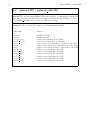
PUMA Flow Diagram
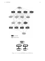
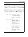
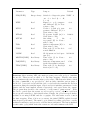
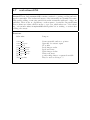
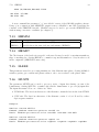
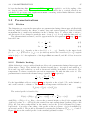
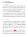
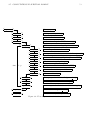
The diagram 9.4 shows the route through the main program PUMA, with the names of the
most important subroutines.
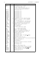
PUMA is the main program. It calls the three subroutines Prolog, Master and Epilog . Prolog
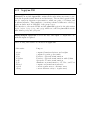
does all initialization. It calls the following subroutines: gauaw computes gaussian abscissas
and weights. inilat initializes some utility arrays like square of cosine of latitude etc. legpri
prints the arrays of gauaw and inilat. readnl reads the namelist from standard input. initpm
initializes most vertical arrays and some in the spectral domain. initsi computes arrays for the
semi-implicit scheme. legini computes all polynomials needed for the Legendre transformation.
restart starts the model from the restart file, if selected of a previous run. initfd initializes
spectral arrays. setzt sets up the restoration temperature array. noise puts a selectable form of
noise into lnP s. setztex is a special version of setzt for dipole experiments.
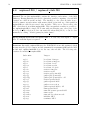
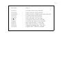
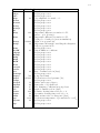
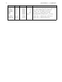
Master does some initial timesteps on initial runs, then it runs the time loop for the selected
integration time. It calls the following subroutines: makebm constructs the array bm, gridpoint
does all transformations and calculations in the grid point domain. sp2fc converts spectral to
Fourier coefficients (inverse Legendre transf.), dv2uv divergence and vorticity to u and v (implies
spectral to Fourier), fc2gp Fourier coefficients to grid points (fast Fourier transformation),
calcgp calculations in grid point space, gp2fc grid points to Fourier coefficients (fast Fourier
transformation), fc2sp Fourier coefficients to spectral (direct Legendre transf.), mktend makes
tendencies (implies Fourier to spectral), spectral does all calculations in the spectral domain,
outsp writes spectral fields in physical dimensions on an output file, and diag writes selected
fields and parameters to the standard output. Epilog writes the restart file.
9.6
Initialization
The model starts either from a restart file or with the atmosphere at rest. The defaults make
the initial state a motionless, stable stratified atmosphere. For an initial start the divergence
and the relative vorticity are set to zero (only mode(1,0) of vorticity is set to the planetary
vorticity). The temperature is initialized as a constant horizontal field. The vertical distribution
is adopted from the restoration temperature, usually a stable stratification. The initialization
of the logarithm of the surface pressure is controlled by the namelist variable kick: kick=0
sets all modes to zero, so the model runs with constant zones without eddies, kick=1 generates
random white noise and kick=2 generates random white noise that is symmetrical about the
equator. Runs started with kick=1 or 2 are irreproducible due to the randomization. For
reproducible runs with eddies use kick=3 which only initializes mode(1,2) of lnP s with a small
constant. The amplitude of the noise perturbation is normalized to 0.1 hPa (1.e-4 of the mean
surface pressure).
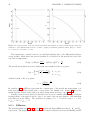
A radiative equilibrium temperature field for the run is set up by setzt: First, a global mean
radiative equilibrium temperature profile TR (σ) is defined. A hyperbolic function of height is
used to provide TR (σ), as illustrated in Figure 9.1. With z → − ∞ the profile tends to a
uniform lapse rate, alr, passing through the temperature tgr at z = 0. With z → + ∞ the
profile becomes isothermal. The transition takes place at the height ztrop. The sharpness
of the tropopause is controlled by the parameter dttrp. When dttrp = 0,the lapse rate
changes discontinuously at ztrop. For dttrp small but positive, the transition is spread. The
hydrostatic relation is used to determine the heights and hence the temperatures of the model
levels.