Download LucidStudio User's Guide

LucidStudio
User's Guide
LucidShape
Computer Aided Lighting
LucidStudio User's Guide
LucidStudio User's Guide
Version 1.12.1
Published July 08, 2014
2
Table of Contents
1. Getting started with LucidStudio ............................................................................................................ 11
1.1. LucidStudio Overview .................................................................................................................. 11
1.2. Principles of LucidStudio ............................................................................................................ 11
1.2.1. Shapes ............................................................................................................................ 13
1.2.2. Views .............................................................................................................................. 14
1.2.3. Mouse Interaction ........................................................................................................... 18
1.2.4. Peculiarities of LucidStudio ............................................................................................. 20
1.3. The First Example: A Guide to LucidStudio .................................................................................. 21
1.3.1. Create an Empty Geometry File ......................................................................................... 21
1.3.2. Create a Cylinder Light Source ......................................................................................... 22
1.3.3. Define a Reflector Surface ............................................................................................... 24
1.3.4. Create Sensors ................................................................................................................ 25
1.3.5. Simulate the scene .......................................................................................................... 27
2. File and Edit ......................................................................................................................................... 31
2.1. Editing LucidShape Documents .................................................................................................. 31
2.2. Saving LucidShape Documents .................................................................................................. 31
2.3. Transferring Geometry between LucidShape and CAD tools ....................................................... 32
2.3.1. The CATIA Transfer Dialog ............................................................................................... 33
2.3.2. The Rhino Transfer Dialog ............................................................................................... 34
2.4. Transformed Input and Output ................................................................................................... 35
2.5. Menu Operations ....................................................................................................................... 35
2.6. Printing ..................................................................................................................................... 36
2.7. Standard Editing ........................................................................................................................ 37
3. Views ................................................................................................................................................... 39
3.1. GeoView .................................................................................................................................... 40
3.1.1. General Commands ......................................................................................................... 40
3.1.2. Selection Modes ............................................................................................................. 40
3.1.3. Viewing Perspectives ...................................................................................................... 40
3.1.4. Clear ............................................................................................................................... 41
3.1.5. Axis ................................................................................................................................. 41
3.1.6. Objects Coloring and Display ........................................................................................... 41
3.1.7. Advanced Display Properties ........................................................................................... 42
3.2. Tree View .................................................................................................................................. 46
3.2.1. Selections ....................................................................................................................... 46
3.2.2. Tree Node Properties ...................................................................................................... 46
3.2.3. Tree Display .................................................................................................................... 47
3.2.4. Elements Display Filtering .............................................................................................. 47
3.3. Text View ................................................................................................................................... 47
3.4. UV View ..................................................................................................................................... 48
3.4.1. General Commands ......................................................................................................... 48
3.4.2. Color Scaling and Scene Lines ........................................................................................ 48
3.4.3. Operations on the Data ................................................................................................... 49
3.4.4. Background Colors .......................................................................................................... 61
3.4.5. Spectral specific options ................................................................................................. 62
3.4.6. Detailed View Properties ................................................................................................ 62
3.5. Light Screen View ...................................................................................................................... 66
3.5.1. General Commands ......................................................................................................... 66
3.5.2. Display Commands ......................................................................................................... 66
3.5.3. Coloring and Display Properties ...................................................................................... 67
3
LucidStudio User's Guide
3.5.4. Screen View Properties ................................................................................................... 67
4. Geometry ............................................................................................................................................. 69
4.1. Basic Operations on Geometric Objects ...................................................................................... 70
4.1.1. Selection, Deletion and Renaming .................................................................................. 70
4.1.2. Transform ....................................................................................................................... 71
4.1.3. Set Global Axis ............................................................................................................... 73
4.1.4. Conversion of Curves and Surfaces .................................................................................. 73
4.1.5. Modify Data Structures of Geometric Objects .................................................................. 73
4.2. Standard Geometries ................................................................................................................. 75
4.2.1. Rectangular Paraboloid ................................................................................................... 77
4.2.2. Rotational Paraboloid ..................................................................................................... 77
4.2.3. Rotational Hyperboloid ................................................................................................... 77
4.2.4. Rotational Ellipsoid ........................................................................................................ 78
4.2.5. Compound Parabolic Concentrator .................................................................................. 78
4.2.6. Cylinder .......................................................................................................................... 79
4.2.7. Sphere ............................................................................................................................ 79
4.2.8. Mesh Sphere .................................................................................................................. 79
4.2.9. Plane .............................................................................................................................. 80
4.2.10. Disk .............................................................................................................................. 80
4.2.11. Cone .............................................................................................................................. 80
4.2.12. Box ................................................................................................................................ 81
4.3. Procedural Surfaces ................................................................................................................... 81
4.3.1. Rotational Surface ........................................................................................................... 81
4.3.2. Pipe Surface ................................................................................................................... 82
4.3.3. Torus .............................................................................................................................. 82
4.3.4. Coil ................................................................................................................................. 82
4.3.5. Extruded Surface ............................................................................................................ 83
4.3.6. Offset Surface ................................................................................................................. 83
4.3.7. Swept Surface ................................................................................................................ 84
4.3.8. Swung Surface ............................................................................................................... 84
4.3.9. Surface from Formula ..................................................................................................... 84
4.4. Standard Curves ........................................................................................................................ 86
4.4.1. Parabola ......................................................................................................................... 86
4.4.2. Hyperbola ...................................................................................................................... 87
4.4.3. Ellipse ........................................................................................................................... 87
4.4.4. Ellipse by Two Focal Points ............................................................................................ 87
4.4.5. Helix .............................................................................................................................. 88
4.4.6. Compound Parabolic Concentrator ................................................................................. 88
4.4.7. Curve from Formula ....................................................................................................... 88
4.4.8. Curve between two Curves .............................................................................................. 90
4.4.9. Curves from NURBS Surface Border ................................................................................ 90
4.4.10. Curves from Trimmed Surface Border ........................................................................... 90
4.4.11. Create Point .................................................................................................................. 90
4.4.12. Create Polyline .............................................................................................................. 91
4.4.13. Create NURBS ............................................................................................................... 92
4.4.14. Create Control Curve ..................................................................................................... 93
4.5. Standard Surfaces ..................................................................................................................... 94
4.5.1. Surface from Boundary Layers ......................................................................................... 94
4.5.2. Surface between Curve and Point .................................................................................... 95
4.5.3. Surface between two Curves ........................................................................................... 95
4.5.4. Surface between two Surfaces ........................................................................................ 95
4
LucidStudio User's Guide
4.6. Lenses ....................................................................................................................................... 96
4.6.1. Aspheric Lens ................................................................................................................. 96
4.6.2. Aspheric Lens Per Formula .............................................................................................. 97
4.6.3. Free Form Fresnel Lens .................................................................................................. 98
4.6.4. TIR (Total Internal Reflection) Lens ................................................................................ 100
4.6.5. Potato Chip Lens .......................................................................................................... 102
4.6.6. Free Form Variable Fresnel Lens ................................................................................... 102
4.6.7. Elliptic Lens ................................................................................................................... 103
4.6.8. Hyperbolic Lens ............................................................................................................ 104
4.6.9. Spherical Lens .............................................................................................................. 105
4.7. Approximated and Interpolated Curve ..................................................................................... 105
4.7.1. Read Point Row ............................................................................................................. 106
4.7.2. Create Fitting Curve ....................................................................................................... 106
4.7.3. Read Value Row ............................................................................................................ 107
4.7.4. Create Explicit Curve ..................................................................................................... 107
4.8. Approximated and Interpolated Surface .................................................................................. 108
4.8.1. Common Dialog Parts .................................................................................................... 108
4.8.2. Read Point Cloud .......................................................................................................... 109
4.8.3. Create Point Cloud ........................................................................................................ 109
4.8.4. Sample Point Cloud from Target Scene ......................................................................... 110
4.8.5. Create Surface from Point Cloud .................................................................................... 111
4.8.6. Read Point Grid ............................................................................................................ 112
4.8.7. Create Point Grid .......................................................................................................... 112
4.8.8. Extrapolate Point Grid ................................................................................................... 113
4.8.9. Sample Point Grid from Target Scene ............................................................................ 114
4.8.10. Create Point Grid on Surface ........................................................................................ 115
4.8.11. Create Fitting Surface .................................................................................................. 115
4.8.12. Read Value Grid .......................................................................................................... 115
4.8.13. Create Explicit Surface ................................................................................................ 116
4.8.14. Create Skinned Surface ............................................................................................... 116
4.8.15. Create Skinned Surface Loft ......................................................................................... 116
4.8.16. Create Skinned Surface Horizontal/Vertical .................................................................. 117
4.9. Ray Deviation Correction ......................................................................................................... 118
4.10. Various Geometry Tools .......................................................................................................... 119
4.10.1. Create Axis System ...................................................................................................... 119
4.10.2. Create Clipping Plane .................................................................................................. 120
4.10.3. Create Object Vector ................................................................................................... 120
4.10.4. Create Polylines from Rays .......................................................................................... 121
4.10.5. Create Cylinder from Rays ............................................................................................ 121
4.10.6. Create Annotation Text ................................................................................................. 121
4.10.7. Create Annotation Bitmap ............................................................................................ 122
5. FreeForm Geometries Menu Selection ................................................................................................. 123
5.1. The menu entries for FunGeo .................................................................................................... 123
5.2. MF Reflector/Lens Surface ...................................................................................................... 124
5.3. Switch Board ............................................................................................................................ 130
5.4. PCS Reflector/Lens Surface ..................................................................................................... 132
5.5. PCS Lens .................................................................................................................................. 137
5.6. Procedural Surface (PS) Reflector ............................................................................................. 138
5.7. Procedural Surface (PS) Refractor ............................................................................................. 141
5.8. Collimator LED Lens ................................................................................................................. 143
5.9. Prismband for Lightguides ....................................................................................................... 149
5
LucidStudio User's Guide
5.10. Dotmask for Backlighting ....................................................................................................... 153
5.11. Retro Reflector ........................................................................................................................ 156
5.12. Genetic Algorithm Optimizer ................................................................................................... 158
5.13. Model Note ............................................................................................................................. 159
5.14. Model Documentation ............................................................................................................ 159
6. Light Sources ...................................................................................................................................... 163
6.1. Base Options and Parameters ................................................................................................... 164
6.2. Classic Light Sources ............................................................................................................... 166
6.2.1. Cylinder Light Source .................................................................................................... 166
6.2.2. Disk Light Source .......................................................................................................... 167
6.2.3. Plane Light Source ........................................................................................................ 167
6.2.4. U-Shape Light Source ................................................................................................... 168
6.2.5. Coil Shape Light Source ................................................................................................ 168
6.2.6. RayFile Light Source ...................................................................................................... 169
6.2.7. Point Light Source ......................................................................................................... 170
6.3. Special Light Sources ............................................................................................................... 170
6.3.1. Volume Light Source ...................................................................................................... 170
6.3.2. LED Point Light Source ................................................................................................... 171
6.3.3. Low Beam, High Beam, Signal Lamp and special Light Sources ...................................... 172
6.4. Sky Light Source ...................................................................................................................... 172
6.5. Ray Trace Bundles .................................................................................................................... 174
6.5.1. Single Ray Bundle ......................................................................................................... 174
6.5.2. Cylinder Filament Bundle .............................................................................................. 174
6.5.3. Free Surface Filament Bundle ........................................................................................ 175
6.5.4. Cone Bundle ................................................................................................................. 176
6.5.5. Parallel Bundle .............................................................................................................. 176
6.5.6. Point Set Bundle ........................................................................................................... 177
6.5.7. Parallel On Normal Bundle ............................................................................................ 177
6.5.8. Tip Cone On Normal Bundle .......................................................................................... 178
6.5.9. RayFile Bundle .............................................................................................................. 178
6.6. RayFile and RayFile Tools ......................................................................................................... 179
6.6.1. The use of a RayFile ....................................................................................................... 179
6.6.2. Simulation with more than one RayFile ......................................................................... 180
6.6.3. Copy RayFile ................................................................................................................. 180
6.6.4. Check RayFile ................................................................................................................ 182
6.6.5. Merge RayFiles ............................................................................................................. 182
6.6.6. Compute a RayFile's Pseudo Focal Point (PFP) ............................................................... 183
6.6.7. Project RayFile on Geometry .......................................................................................... 184
6.6.8. Lamp Models for RayFiles ............................................................................................. 184
7. Emitter, Actor and Sensor Materials .................................................................................................... 187
7.1. The Dialogs Create Material and Assign Material ...................................................................... 187
7.2. Emitter Materials ..................................................................................................................... 189
7.2.1. Lambertian Emitter ........................................................................................................ 190
7.2.2. Directional Emitter ........................................................................................................ 190
7.2.3. Isoradiant Emitter .......................................................................................................... 191
7.2.4. Ray File Emitter ............................................................................................................. 191
7.2.5. LID File Emitter .............................................................................................................. 191
7.2.6. LID Curve Emitter ........................................................................................................... 191
7.2.7. LID Surface Emitter ........................................................................................................ 192
7.2.8. Spectral Power Distribution (SPD) ................................................................................. 192
7.3. Actor Materials ......................................................................................................................... 194
6
LucidStudio User's Guide
7.3.1. Ideal Mirror (Reflective) ................................................................................................. 198
7.3.2. Ideal Lens (Refractive) ................................................................................................... 199
7.3.3. Lambertian (Reflective and Refractive) .......................................................................... 199
7.3.4. Gaussian (Reflective and Refractive) ............................................................................. 200
7.3.5. Gaussian Retro-reflex (Reflective) ................................................................................. 200
7.3.6. Lambert/Gauss Combination (Reflective and Refractive) ............................................... 200
7.3.7. 2D BSDF Theta Curve (Reflective and Refractive) ........................................................... 201
7.3.8. 3D BSDF data from file (Reflective and Refractive) ......................................................... 201
7.3.9. ABg (Reflective) ............................................................................................................ 201
7.3.10. Absorber ..................................................................................................................... 202
7.4. Sensors and Sensor Materials ................................................................................................. 202
7.4.1. Candela Sensor ............................................................................................................. 204
7.4.2. Ray File Sensor ............................................................................................................. 206
7.4.3. Ray History Sensor ....................................................................................................... 206
7.4.4. Volume Sensor ............................................................................................................. 207
7.4.5. Light Flow Sensor ......................................................................................................... 208
7.4.6. Exit Sensors .................................................................................................................. 210
7.4.7. Illumination (Lux), Light Flux (Lumen) and Luminance (Candela per m2) Sensor Materials .......................................................................................................................................... 210
7.4.8. Luminance Camera ........................................................................................................ 212
7.4.9. License Plate Sensor ..................................................................................................... 215
7.5. Media for Refractive Materials .................................................................................................. 217
7.6. Spectral Reflection, Refraction and Absorption Distributions .................................................... 219
7.6.1. User Defined Spectral Distributions ............................................................................... 219
7.6.2. Special Dispersion and Emission Functions ................................................................... 220
7.7. The BSDF Wizard ..................................................................................................................... 224
7.7.1. BSDFs in a nutshell ....................................................................................................... 224
7.7.2. The Wizard's Dialog Elements ....................................................................................... 225
7.8. Importing other BSDF Data ..................................................................................................... 227
7.9. Set Colour ............................................................................................................................... 228
7.10. Set Texture ............................................................................................................................ 228
8. Simulation .......................................................................................................................................... 231
8.1. Monte Carlo Ray Trace .............................................................................................................. 231
8.2. GPU Trace Simulation .............................................................................................................. 235
8.3. Light Mapping Simulation ........................................................................................................ 236
8.4. Simulate by Spooler ................................................................................................................ 237
8.5. Simulation Manager ................................................................................................................ 239
8.6. Sensor Light Calculations ......................................................................................................... 241
8.6.1. Gather Sensor Light ....................................................................................................... 241
8.6.2. Reverse Sensor Light .................................................................................................... 241
8.6.3. Luminance Image Sensor Light ..................................................................................... 242
8.7. Various Commands .................................................................................................................. 244
8.7.1. Random Rays ................................................................................................................ 244
8.7.2. Interrupt ....................................................................................................................... 244
9. Analysis of Geometry and LID Data ..................................................................................................... 245
9.1. LID Measuring .......................................................................................................................... 245
9.1.1. Apply Test Tables .......................................................................................................... 245
9.1.2. Apply Last Selected Test Table ...................................................................................... 248
9.1.3. Measure Point or Zone .................................................................................................. 248
9.2. LID Modeling ........................................................................................................................... 249
9.2.1. Trim Cutoff Lines ........................................................................................................... 249
7
LucidStudio User's Guide
9.2.2. Interpolate LIDs from Test Tables ................................................................................. 250
9.3. LID Data Conversion ................................................................................................................. 251
9.3.1. Surface from LID Data .................................................................................................... 251
9.3.2. Section Curve through LID Data .................................................................................... 253
9.4. Analysis of 3D Geometry .......................................................................................................... 255
9.4.1. Bounding Box ............................................................................................................... 255
9.4.2. Visualize Volume Sensor .............................................................................................. 255
9.4.3. Restore Rays from Ray History Sensor .......................................................................... 257
9.4.4. Ray Deviations and Checkerboard Images ..................................................................... 260
9.4.5. Wall Thickness Diagram ................................................................................................ 262
9.5. Benchmark test tool for TC4-45 or self defined assessments .................................................... 264
9.6. Bitmap Tools ........................................................................................................................... 267
9.6.1. Bitmap Show ................................................................................................................ 267
9.6.2. 3D Snapshot ................................................................................................................. 268
10. LIDEditor ........................................................................................................................................... 269
10.1. Overview ................................................................................................................................ 269
10.2. LID Editor Gallery ................................................................................................................... 269
10.3. LID Editor ............................................................................................................................... 270
10.3.1. Loading LIDs ................................................................................................................ 270
10.3.2. Options and Parameters .............................................................................................. 270
10.3.3. Editing LIDs ................................................................................................................. 272
10.4. Dynamic LID Editor ................................................................................................................. 274
10.4.1. Introduction and Principle ............................................................................................ 274
10.4.2. Example ...................................................................................................................... 275
11. Applications ...................................................................................................................................... 277
11.1. General Automotive Application .............................................................................................. 277
11.1.1. Static Road Simulation ................................................................................................. 277
11.1.2. Virtual Beam Pattern .................................................................................................... 282
11.1.3. License Plate ................................................................................................................ 283
11.1.4. Retro Reflector ............................................................................................................. 284
11.2. General Application ................................................................................................................ 285
11.2.1. Aircraft Lighting ........................................................................................................... 285
11.2.2. Test Room for Indoor Lighting ...................................................................................... 286
11.2.3. Street Illumination ....................................................................................................... 287
11.2.4. Reverse Street Light Pattern Calculation ...................................................................... 294
11.3. Tests ...................................................................................................................................... 296
11.3.1. BSDF Maker ................................................................................................................. 296
12. Miscellaneous Menus ....................................................................................................................... 299
12.1. Custom ................................................................................................................................... 299
12.2. Options .................................................................................................................................. 299
12.2.1. Global Settings ............................................................................................................ 299
12.2.2. Working Directory for Open/Save ................................................................................ 301
12.2.3. Editing of LID Test Tables ............................................................................................ 302
12.2.4. Hardware Graphics Accelerator ................................................................................... 302
12.2.5. COM Server ................................................................................................................. 302
12.3. Window .................................................................................................................................. 303
12.4. Help ....................................................................................................................................... 303
12.4.1. License Check .............................................................................................................. 304
12.4.2. Shortcuts to LucidShape Documents ........................................................................... 304
A. LucidShape File Types ........................................................................................................................ 305
B. List of Toolbar Icons ........................................................................................................................... 307
8
LucidStudio User's Guide
B.1. Common Tools ......................................................................................................................... 307
B.2. View Options and Manipulation Tools ...................................................................................... 307
B.3. Simulation and Script Execution Tools ..................................................................................... 307
B.4. Geometry View Tools ............................................................................................................... 308
B.5. UV/Light Data View Tools ........................................................................................................ 308
C. Mouse Interaction Reference .............................................................................................................. 309
C.1. Geometry View ......................................................................................................................... 309
C.2. Tree View ................................................................................................................................ 309
C.3. Light Screen View .................................................................................................................... 309
C.4. UV/Lightdata View ................................................................................................................... 310
C.5. Text Edit View .......................................................................................................................... 310
C.6. Message Box ........................................................................................................................... 310
D. Efficacy Scale Factor and Rhino CAD Im-/Export .................................................................................. 311
D.1. Efficacy Scale Factor ................................................................................................................. 311
D.2. Materials Import/Export: Rhino CAD ........................................................................................ 312
Index ...................................................................................................................................................... 313
9
10
Chapter 1. Getting started with LucidStudio
1.1. LucidStudio Overview
LucidStudio is the interactive interface to the LucidShape design system. Its graphical user interface
follows Microsoft Windows® standard and is thus intuitive, user friendly, and easy to learn and
master. It allows all design tasks to be performed at a mouse click.
State of the art computer graphics (OpenGL) are used for the 3D scene views, allowing an easy and
fast navigation within the scene. Tree views provide an overview of the light simulation scene and
simplify the procedure of modifying objects and properties. "UV data" views display light data and
other value distributions over a 2D UV parameter range.
LucidStudio also offers a number of analyzing tools: interactive ray path analysis, curvature analysis
for surfaces, smoothness filters, and gradient analysis of light data, to name a few.
Being a Windows application, LucidStudio is primarily operated with a mouse, but its LucidShell
interface makes it easy to extend functionality to adapt the applications to your special needs. You
write your own tool in the LucidShell language and run it simply by clicking from within LucidStudio.
This documentation has two purposes: it introduces you to the use of LucidStudio, and it serves
as a reference handbook in your daily work.
It is assumed that you know about optics and lighting and its terminology. Unique definitions of
the terminology used in this handbook are given in the glossary. It is also assumed that you are
acquainted with the standard Microsoft Windows® dialogs like Open File. If this does not fit you,
we recommend you to first read the help texts accompanying e.g. the standard Microsoft Windows®
Wordpad Editor.
To start, please take a look at the next section of this chapter on the principles of LucidStudio. It
treats important aspects of the GUI, operational concepts of LucidStudio, and the special terminology
that is used throughout this manual. After that, you can follow the example given in the last section
of this chapter. It was created for a quick start and guides you through the common steps of creating
an optical setup in LucidStudio. Once you are familiar with the basic steps, you can modularly increase the repertoire of commands you apply.
Therefore the following chapters describe all menu items of LucidStudio step by step. The commands
available to you within each menu are explained and their application dialogs are addressed in
detail.
1.2. Principles of LucidStudio
This chapter will guide you through the basic operational concepts of LucidStudio and give some
insight in what the important structures of its GUI are. It will tell you about the concepts of experiment description, i.e. how light sources or sensors are defined. You also learn about the different
views on an experiment that LucidStudio offers. The available mouse interactions and special
properties of LucidStudio will also be addressed. Let's start with a glance at the terminology.
11
Getting started with LucidStudio
Whether you consider it a scene you are setting up or an optical system you want to design:
Whenever a complete setup is approached, it is called the "Experiment". Every experiment consists
of active parts and sometimes also passive parts. The active parts are visible to the simulation and
are participating in the outcome of the simulation (e.g. ray-tracing), passive parts are not (→ VPT).
The active elements are called "Shapes" in LucidStudio. So what are "shapes"? A shape is a
combination of geometry and material, so this object has a form and a behaviour in LucidStudio.
Thus the shape is one of the fundamental concepts of LucidStudio and is discussed in detail in the
following sections. Passive parts of an experiment do not influence the outcome of it directly. They
can be data you stored or material properties you designed for later use or anything else. Basically,
we divide everything that is part of your experiment into shapes and non-shapes.
The "Geometry" is another basic concept. Every active element you want to design must possess
a geometry in order to exist. The geometry is therefore a property of any shape. It can be a 2D or
3D geometrical object like a curve or a surface or a cylinder, but also a single point is considered
a valid geometry. Geometries can also be exchange data from and to external CAD software. Please
note that a pure geometry without further properties will be considered as a passive element and
therefore is not a shape.
The "Material" is the second property of a shape. Whether you define a light-source or a lens, for
example, any valid shape must also consist of a material. For convenience, the material properties
available within LucidStudio are split up into the three classes of emitters, actors and sensors.
"Sensors" are to some extend an exception to the other elements within LucidStudio. They are not
only a material property but can be stand-alone entities themselves. In that case, they still possess
a geometry, but it will be of infinity-type, e.g. an infinitely distant or infinitely large detection area.
This is usually pre-defined for such a sensor type. In consequence, not all available sensors of
LucidStudio can be attached to finite geometries.
The "Views" of LucidStudio are separate windows that show different parts or aspects of your experiment. Thus, they serve different purposes for design or analysis of your optics setup. Views
can be considered the main user interfaces of LucidStudio and are dealt with in Section 1.2.2,
“Views”.
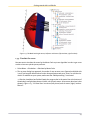
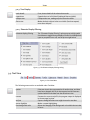
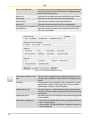
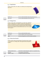
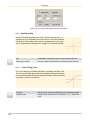
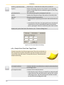
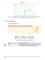
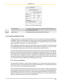
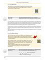
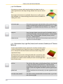
Almost every object in LucidShape has four "Attributes" (or flags) : Editable (E), Visible (V), Pickable
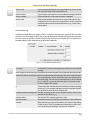
(P) and Traceable (T). An exemplary TreeView is shown in the picture below (see Figure 1.1, “The
Model Tree View (with marked EVPT flags)”). All four flags can be toggled pressing Ctrl+Shift+Letter,
just mark a shape, highlight either the Geo- or the TreeView and press the respective hot key.
"Editable" is kind of a protection against accidental changes. If unchecked, the respective shape
can be examined (to see the options and parameters), but it cannot be altered. To change the values
just enable the flag "E" and open the edit dialog as usual.
"Visible" determines whether this object is visible in the geometry view or not (used to enhance
the clarity in more complex models). If "Pickable" is checked the respective object is pick-able in
the geometry view, this can be set off to make it easier to mark and grab single objects. The fourth
attribute is "Traceable". If checked this object takes part in the light simulation, if unchecked it is
not traced in the ray-trace process (kind of 'invisible' for the rays, not to be mismatched with 'V'
in the geometry view!). Every single attribute can be set independently to the other three, if an
object is neither visible nor pick-able it still takes part in the light simulation as long as it is traceable.
12
Getting started with LucidStudio
1.2.1. Shapes
Experiments in LucidShape consist of "Shapes". A "Shape" is an object that takes part in the
lighting experiment. It may be one of the following types:
• Light emitting devices, called "Emitting Shapes" or "Lightsources" in LucidShape's terminology.
• Objects that change incoming light by refracting, reflecting or absorbing it. These objects are
called "Actor Shapes" or simply "Actors".
• Light measuring devices, called "Sensor Shapes" or simply "Sensors".
Any shape consist of two properties: Geometry and Material. To create a shape, you have to add
one or more material properties to an already existing or newly created geometry.
Geometry
In LucidShape, a geometry object defines a certain region in space. It will be displayed in the geometry view, but unless it is part of a shape it will be invisible to the simulation. You can choose
from a variety of pre-defined geometrical objects or create any object you need from scratch.
Material
Emitters
A shape of light source type is created, if an emitter material property is attached to a geometry.
For modelling voluminous light sources like gas discharge lamps, simply define an enclosing surface
with an emitter property.
Actors
An actor is also a material property attached to a geometric surface. You can define an actor to be
an absorber, a reflector or a refractor. Reflectors can be ideal (i.e. 100% reflectance) or of more
realistic quality. They can be perfectly specular, purely diffuse or may provide any ratio of scattering
in between. A refractor may either be an ideal refractor or a Fresnel refractor (where a part of the
incoming light will be reflected). To model a refractive optical medium that occupies a certain
volume in space, define its outer surfaces with the corresponding refractive indices. Transmission
losses, however, will not be modelled. They may be accounted for by using a scale factor, either
with the light source, the refractive material or the sensor. You may also apply an absorption
coefficient to the refractive material to model transmission losses. You will find detailed descriptions
on the creation of available actor material properties in Chapter 7, Emitter, Actor and Sensor Materials.
Sensors
There are several types of sensors available. The main ones are: luminous intensity (candela), illumination (lux) or light flux (lumen) sensors. Sensors consist of a number of equally sized cells distributed across the supporting surface. The resolution of the sensor can be chosen by increasing
or decreasing the number of cells. Also certain data files can be treated as a sensor.
13
Getting started with LucidStudio
1.2.2. Views
The experimental setup can be approached in six different ways:
•
•
•
•
•
•
the section called “Model Tree View”
the section called “Geometry View”
the section called “Light Screen View”
the section called “ UV Data View”
the section called “ Script and Text View”
the section called “Message View”
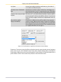
Model Tree View
Figure 1.1: The Model Tree View (with marked EVPT flags)
In the model tree view, or simply the "tree", a textual representation of all objects in the setup and
all their hierarchical dependencies are displayed. The Figure 1.1, “The Model Tree View (with marked
EVPT flags)” above shows an example of the compact tree view. Once you select an entry, the object
is highlighted also in the geometry view. For example, a simple cylindrical light-source (shape)
enlisted in the tree would be linked to two further entries: A CylinderSurface (geometry) and a
LambertEmitter (material). Even in complex experiments, you will be able to quickly identify and
select one or several elements within the tree. If dialog boxes are implemented in the setup, they
can be started by double mouse click directly from the tree.
Geometry View
The geometry view displays the geometric parts of your experimental setup in 3D (switchable to
2D planes), e.g. surfaces of reflectors, refractors, light sources, and detector geometries. It is also
possible to display certain kinds of data associated with a surface, e.g. surface curvature or illumination data of a sensor. Also in this window, the geometry can be analyzed by using interactive ray
trace.
14
Getting started with LucidStudio
For good orientation, an axis system is visualized. Furthermore, you can zoom objects and change
between different display types like light data, shaded, black & white, and wire frame. Objects can
be selected by double clicking (left) with your mouse. You can for example also choose between
selecting geometries only or the complete shape (see. Section 1.2.3, “ Mouse Interaction”).
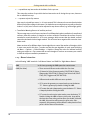
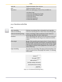
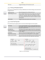
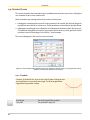
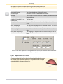
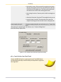
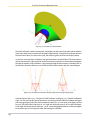
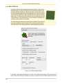
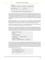
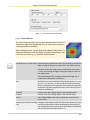
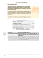
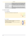
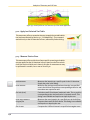
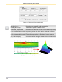
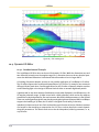
A good example of the geometry view is shown in Figure 1.2, “The Geo View”. The experiment on
display consists of two lenses, one of them surrounded by a shield, a light-source and a parabolic
reflector. A ray bundle has been drawn to visualize the imaging and the vertex of the reflector has
obviously been placed in the center of the coordinate system. The display mode was chosen
"shaded".
Figure 1.2: The Geo View
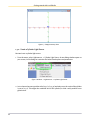
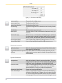
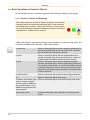
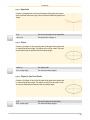
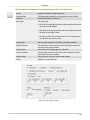
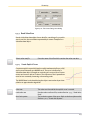
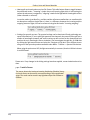
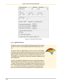
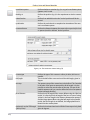
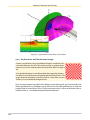
Light Screen View
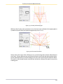
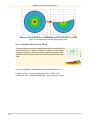
The light screen displays filament images or ray target dots during the interactive ray trace analysis
(see. the section called “ Interactive Ray Trace”). An angular coordinate system A or B, or on the
plane Z at a specific position can be chosen. It is a very useful tool to ensure correct imaging and
image orientation. It also can assist e.g. in estimating the impact of alterations to your optical
system before doing a complete simulation.
Figure 1.3: The Light Screen View
15
Getting started with LucidStudio
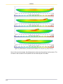
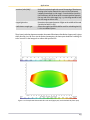
The light screen shown in Figure 1.3, “The Light Screen View” features cylindrical filament images
from four different ray bundles (i.e. four separate images). During the interactive ray path analysis,
any change in the optical setup directly affects these images according to the ray bundles you had
previously defined. Therefore you can immediately see the impact of your modifications. Please
note that the images are directly obtained from interactive ray tracing and do show different sizes
correctly as a result of the actual imaging system and the path of the traced ray bundles.
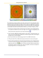
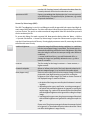
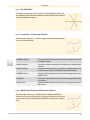
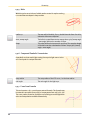
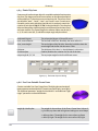
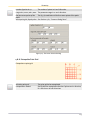
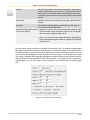
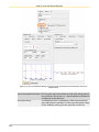
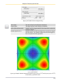
UV Data View
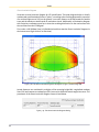
The UV data view offers the best support for viewing scalar data like light intensities on a surface.
The data are displayed according to local coordinates ("u,v"-coordinates) on the surface and they
are color coded. Several analysis methods for the data are available, e.g. iso lines, smoothing (filtering), linear or logarithmic scaling.
Figure 1.4: The UV Data View
Script and Text View
The text view shows a textual representation of the experimental setup as it is contained in the
file. It provides you with all the information on the experiment, all the implemented shapes, and
ray-tracing data as well. In the text view, complete control of the objects' parameters is possible.
It is therefore recommended for experienced users of LucidShape and LucidShell. The script view
is a textual representation as well, but it is used for script files with file name extension "*.do" or
"*.hdo". The main feature of a script view is the "execute" functionality.
16
Getting started with LucidStudio
Figure 1.5: The Text View
Message View
The message view is a text view used for displaying log messages. It is strongly recommended to
keep the message window always open in your work space. Errors can most easily be located by
examining the log messages. All log output is also stored in a file called "LucidShape.log".
Figure 1.6: The Message View
Beside error and warning messages, there are four common messages concerning simulation results:
• ... rays stopped because of a trace level > 'recursion'
This means that the stated number of rays have been stopped because they have reached their
limit of intersections (recursion).
• ... rays stopped because of an intensity < 'intensity level'
A ray will be considered as absorbed (and stopped tracing) if its 'intensity level' is smaller than
a given critical value (mainly due to absorption processes).
• ... rays reached shape (i.e. absorber) without outgoing ray
A ray has reached an absorber and will not traced any further.
17
Getting started with LucidStudio
• ... rays without any intersection in the Monte Carlo ray tracer
This states the number of rays which had no intersection at all during the ray trace, these are
the so-called direct rays.
• ... rays were rejected by sensors
Here a ray is rejected by a sensor, i.e. it is not counted. This is because its current refractive index
differs from the the settings in the sensor. Per default a sensor only detects rays with a refractive
index of 1.0 (air), but of course it can be adjusted to any other medium (e.g. inside a light-guide).
• Tessellation Warning: Ran out of auxiliary vertices!
This message may occur in former versions of LucidShape during the tessellation of complicated
surfaces, when the number of triangles or vertices needed to tessellate the surface correctly
exceeded a certain threshold. It is an error message, which means that the related surfaces
cannot be simulated via the triangle method. This of course has a negative effect onto the simulation result.
Newer versions of LucidShape have a better algorithm to control the number of triangles, which
in most cases avoids this error. To make sure that the new algorithm is used, open the dialog
via Menu → Options → Global Settings → Graphics. Change the value for maximal auxiliary
nodes per surface to 0. Zero means that as much triangles or vertices as necessary are created
to fulfil the surface tessellation parameters 1.
1.2.3. Mouse Interaction
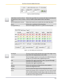
In the following 'LMB' stands for 'Left Mouse Button' and 'RMB' for 'Right Mouse Button'.
RMB
In all views, pressing the RMB opens the context menu
LMB (Geo View)
• There are tree different modes within the Geo view:
• G) Normal or Select Geometry mode (G BUTTON), S) Select
Shape mode (S BUTTON), P) Select Pivot Point mode (P BUTTON), ESC) Toggle mode (ESC BUTTON).
• Different mode enable different cursor symbols.
• G) To enter the geometry or normal mode, press the button
"G". Select a geometry by double-clicking the LMB.
• S) To enter the select shape mode, press the button "S". Select
a shape by double-clicking the LMB.
• P) To enter the select pivot point mode, press the button "P".
Double-clicking the LMB to select a pivot point. A ray will be
shot into the scene at the position where you double-click with
the LMB; this position will become the pivot point. Subsequently, the geometry will be shifted in a way that the Pivot
point is at the center of the window.
18
Getting started with LucidStudio
• ESC) By pressing the ESC button, one can toggle between the
different modes.
LMB: Select (Tree View)
If you select an entry in the tree view, the object will be highlighted in the geometry view.
LMB: Select (Data View)
In data view, after pressing the LMB, you enter the value display
mode. Point to a position or move the mouse while keeping
pressed the LMB. The value of the current position is displayed
in the window's entry bar.
LMB: Select (Light Screen View) In light screen view, after pressing the LMB, you enter the position
display mode. Point to a position or move the mouse while
keeping pressed the LMB. The current position is displayed in the
window's entry bar.
Double-Click on LMB: Select
(Geometry View)
Selecting an entry in the geometry view. Depending on the modus
(G,S or P) a geometry, a shape or a Pivot point. The selected
geometry or shape is highlighted.
Selecting another entry in the geometry view. Depending on the
<SHIFT> plus Double-Click on
LMB: Another Select (Geometry modus (G,S or P) a geometry, a shape or a Pivot point. The selected objects are highlighted.
View)
<CTRL> plus LMB: Another Select Selecting another entry in the tree view. The selected objects are
highlighted.
(Tree View)
<SHIFT> plus LMB: Select Region When you select two entries in the tree view, both entries and all
entries between them are highlighted.
(Tree View)
LMB: Rotate (Geometry View)
In the geometry view, after pressing the LMB, the rotation mode
is started: Move the mouse while keeping pressed the LMB to
rotate the scene.
<SHIFT> plus LMB: Zoom Model This combination starts zoom mode in geometry, data and light
screen view.
(Geometry & Data & Light
Screen View)
• Zooming in: moving the mouse upwards while keeping pressed
<SHIFT> and LMB.
• Zooming out: moving the mouse down while keeping pressed
<SHIFT> and LMB.
<SHIFT> and <CTRL> plus LMB:
Zoom Rectangle (Geometry &
Data & Light Screen View)
To draw a zooming rectangle, press both <SHIFT> and <CTRL> together with the LMB. Releasing zooms with the rectangle as view.
Available in geometry, data and light screen views.
<CTRL> plus LMB: Interactive Ray This combination defines an interactive ray trace: A light ray is
emitted from given start point(s). The initial direction of the light
Trace (Geometry View)
ray is given by the line(s) from the start point(s) to the point of
the surface the mouse points to. If the mouse points into a geometry-free region, no light ray will be emitted.
<CTRL> plus Double-Click on
LMB: Interactive Ray Trace
(Geometry View)
Freezes the current traced ray path.
19
Getting started with LucidStudio
Middle (Wheel) Mouse Button In geometry or data view, you can pan (move left/right and
or Left and RMB: Panning (Geo- up/down) the scene by using the middle mouse button (or the
left and right button simultaneously). In both views, this is a twometry & Data View)
dimensional movement on a plane parallel to the viewer.
Pressing the RMB in the geometry view while holding <SHIFT>
<SHIFT> and RMB (Geometry
View): Display Coordinate Sys- pressed displays a little coordinate system at the point of the
surface the mouse points at. Two axis of the coordinate system
tem
visualize the tangents of the two coordinate lines (red=u,
green=v). The third, blue, is the normal.
<CTRL> plus Middle (Wheel) But- After pressing <CTRL> and the middle (wheel) button (or left and
right button simultaneously), the ray trace start position of bundle
ton or Left and RMB
rays is moved. This only works if rays have already been frozen,
see: Interactive Ray Trace (Geometry View).
Mouse Wheel (Geometry and
Data View): Zoom In and Out
Within the geometry and the data view, one can zoom in and out
by moving the mouse wheel in upper (zoom in) or lower (zoom
out) direction.
1.2.4. Peculiarities of LucidStudio
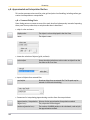
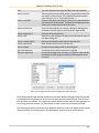
Dialog Box Techniques
Most dialogs offer you to assign something to an existing object or to choose one or several objects
or external data files for the intended operation. These dialogs always follow the same sequence.
In dialogs with "sel" buttons (object selection buttons), first click the button. A new dialog box
with "sel done" appears. When you have selected the object you desire, press the "sel done"
button and the dialog will close. This is the standard procedure for this type of dialog selection.
For dialogs with "..." for file selection, files are selected by pressing the file selection button "...".
A file selection box appears where you enter a file name or select the required directory. When you
have finished selecting the file or required directory, press the "Open" button.
Color selection works in the same way, but the dialog selection is compelled with the "OK" button.
Script integration
One of the basic concepts of LucidShape is that scripts can be easily integrated. If you need to extend
LucidShape's functionality, simply write a script to do the task. There is also a script interface to
interactive dialogs, and you can integrate your own script functions in the menu tree of LucidStudio.
The task "Test Scene" (from the Tests menu) is an example for an interactive script function.
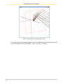
Interactive Ray Trace
An important and powerful feature is the interactive ray trace. It allows you to check the optics of
your experiment in an instant. The displayed ray traces are created by so called "ray trace bundle"
objects. The bundle starts at the current ray start position (set in "Properties" dialog box) and goes
over the current "touched" surface. The default is one single ray only. For different purposes, you
can have different types of bundles, i.e. a filament bundle or a parallel bundle. You may create
them with the dialog from the default task file. Also you may edit them in a separate file and add
the file to your geo-view with "Add file" or "Add recent file".
20
Getting started with LucidStudio
You can ask for a light screen view. This view displays the images (filaments or set of dots) of the
ray path bundles on a 10m screen.
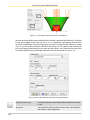
1.3. The First Example: A Guide to LucidStudio
In this section, we will guide you through a simple example of the design of an optical system in
LucidStudio. Keep in mind, that we need at least three different shapes: one light-source, one actor
and one sensor. We will build a lighting experiment that consists of:
• one cylinder light source,
• one parabolic reflector,
• and two sensors.
There are two ways to create this example system. You can start a semi-automatic sequence of
what has to be done to set up the experiment - or you can follow the instructions in this chapter
and do all the necessary steps manually. You can run the automated example via the main menu:
Tests → Test Scene.
After that, you may always hit the return/enter button or press the apply button in the dialog with
every new dialog that appears, and you will have finally created the scene. The window that appears
after the first dialog shows the geometry where you see the model in front view. To change the size
press SHIFT and the LMB simultaneously in upper (increase) or lower (decrease) direction. You
may rotate the model by pressing the LMB and simultaneously move the mouse inside this window.
This view is called the "Geometry View". The cylinder light source is drawn in yellow or the color
you have selected. To move the model inside the window press the left and the right buttons simultaneously and move the mouse. After all dialogs have been applied, you can proceed with a
simulation.
It is more educational to select all menu items manually and create the example yourself. We will
guide you through this process step by step. You will be able to understand and use some of the
necessary procedures and dialogs intuitively. If so, you may quickly go through the steps you
already can handle and proceed. Other tasks may be more complex and you will not be familiar
with these. However, this chapter focuses on the creation of the example above. It will not teach
you all the details and the variety of options in LucidStudio. But it presents you a task where you
can follow a fundamental design sequence that is considered representative for the principles of
use of the LucidStudio software.
1.3.1. Create an Empty Geometry File
To start with, we first start LucidShape and create an empty geometry file.
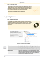
1. Choose "File → New" from the menu and then select "geometry" from the emerged Document
Type dialog. A blank window with a coordinate system appears, it should be similar to this:
21
Getting started with LucidStudio
Figure 1.7: Empty Geometry View
1.3.2. Create a Cylinder Light Source
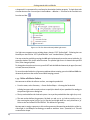
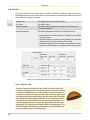
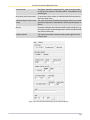
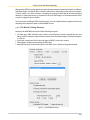
Next we insert a cylinder light source.
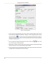
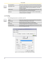
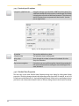
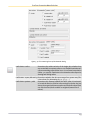
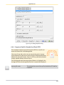
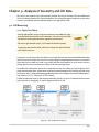
1. From the menu, select Lightsources → Cylinder Light Source. A new dialog window opens on
your screen, in this dialog we customize the below listed options and parameters.
Figure 1.8: Menu → Lightsources → Cylinder Light Source
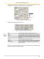
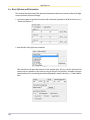
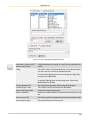
2. Let us choose the source position to be (x,y,z) = (0,0,30) and make sure, the z-axis of the cylinder
is set to (0,0,1). This aligns the rotational axis of the cylinder (its local z-axis) parallel to our
global z-axis.
22
Getting started with LucidStudio
Figure 1.9: The Cylinder Light Source Dialog with the customized Options and Parameters
3. Set the length to 5 and the radii to 0.5.
4. The default display color for light-sources is yellow (255,255,0), of course it can be modified via
changing the three numbers of the RGB code or select the color table via "...".
5. Check "create ray bundle" at the bottom with the ray bundle for interactive ray-trace dialog to
be able to do interactive ray trace later. Alternatively, with "grid on touch surface" you could
create a u by v grid where the rays touch the surface. But for now, we will use the ray bundle
only.
6. Now switch to the right tab of this dialog, as emitter type we choose a lambertian emitter and
set the flux to 1000 lm.
7. Enter a source name, let us take "Cylinder Light Source" and click on <Create>.
After pressing Create the geometry view will automatically be updated. It now contains a cylinder
positioned at x=0, y=0, z=30. We see the model in front view, so it should look like a circle. Please
note, what you see in the geometry view is its geometrical part, i.e. its surface. The light source is
23
Getting started with LucidStudio
a shape and it is represented by a surface plus the attached emitter property. To check that, take
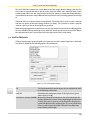
a look at the tree view. You can open it via the Menu → Window → Tree View or the TreeView Icon
from the tool-bar:
.
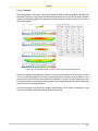
Figure 1.10: The Tree View with newly added Light-source
Our light-source appears as an emitting shape, denoted "VPT SurfaceLight". Following the tree
hierarchy we also find the "VPT CylinderSurface" and "LambertEmitter" properties.
You may rotate the model by pressing the LMB and simultaneously move the mouse inside the 3D
geometry window. This view is called Geo view. The cylinder light source is drawn in the specified
color (if not changed yellow).
To change the size and zoom in or out, press SHIFT and the LMB simultaneously in upper (increase)
or lower (decrease) direction.
To move the model inside the 3D geometry window without rotating, press the LMB and RMB simultaneously and move the mouse around while keeping pressed.
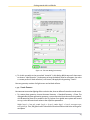
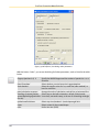
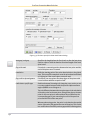
1.3.3. Define a Reflector Surface
Now we want to define the reflector surface, a rectangular paraboloid.
1. From the menu, select Geometry → Create Surface Shape → Rectangular Paraboloid.
A dialog box opens with several sections to specify the details of your paraboloid in analogy to
the previous light-source dialog box.
2. The top section defines the local axis system. Let us put the paraboloid at the origin (x=y=z=0).
3. The next section defines the geometry. Set both xmin and ymin to -50, both xmax and ymax to 50,
thus covering the region [x]=[y]=[-50,50]. Set the focal length both in x- and y-direction to 30.
Select a color and a name for the reflector. This defines the geometry.
Next we want to assign a property to this surface geometry: We want the paraboloid to reflect incident light, in LucidShape's terminology, we want to attach an "actor" (material) to it. This will
create an actor shape.
24
Getting started with LucidStudio
Figure 1.11: The main Dialog for Geometry
4. To do this we switch to the second tab "material" in this dialog. Within we scroll down menu
we choose "Ideal Specular". Furthermore we keep the default value for reflectance, the value
1.0 means perfect or ideal reflection (= 0% losses). We apply this by pressing "Create".
Now our geometry consists of a light source and an ideal reflector.
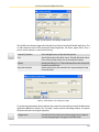
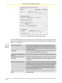
1.3.4. Create Sensors
Next we want to see what lighting effect our device has, thus we define a first and a second sensor.
1. To create a plane geometry, choose the menu Geometry → Standard Geometry → Plane. The
dialog window for plane geometries opens up, to some extent similar to the one for the paraboloid. We want the plane to be parallel to the (x,y)-plane of our global axes system and located
at z=50, to do this enter these values to the respective parameters:
Origin (x,y,z) = (0,0,50); z-axis (x,y,z) = (0,0,1); x-axis (x,y,z) = (1,0,0); xmin=ymin=-50;
xmax=ymax=50. Thus, the global z-axis is the also the direction of the normal vector of the generated plane.
25
Getting started with LucidStudio
2. As we want this plane to be a sensor, we press "Create Shape", switch to the sensor tab and
choose "Sensor for Illumination [lx]" in the scroll down menu. In the detector setting, we set
the cell size to 1 and keep the rest of the default settings. Press "Create" to create our lux sensor.
3. Next we create a luminous intensity distribution sensor. Select from the menu Sensors → Candela
Sensor. Use the default values and confirm them by pressing "Create", a candela sensor is created.
Figure 1.12: The Candela Sensor Dialog
Please note, this [cd] sensor differs from the [lx] sensor: it is neither attached to the plane you
just created, nor any other of your geometries. The candela sensor requires an infinity surface
geometry (check tree view!). Thus, it is not allowed to assign the candela sensor to an arbitrary
finite surface.
⇒ Now our experimental setup is complete, we have an emitter, an actor and at least one sensor.
The GeoView and the TreeView respectively should now look similar to this:
26
Getting started with LucidStudio
Figure 1.13: The Model with Light-source, Reflector and Sensor (left GeoView, right TreeView)
1.3.5. Simulate the scene
Now we want to simulate the scene by the Monte Carlo ray trace algorithm in order to get some
results on how our optical system performs.
1. Select Menu → Simulation → Simulate by Monte Carlo.
2. The ray trace dialog has appeared. As number of rays we enter 2000 (internal multiplied with
*1000), but keep the default values for the other parameters and press "Start" to start the simulation. If available on your system, make sure that "Multiprocessing" is activated.
⇒ After the simulation has finished (watch the progress bar in the status line at the bottom of
the window), two light data views are visible, one for each sensor. A lux sensor data view is also
shown in Figure 1.15, “UV Data View: lux sensor (left picture) and cd sensor (right), both unfiltered”.
27
Getting started with LucidStudio
Figure 1.14: Ray Trace Dialog
3. In case you have closed a light data view, choose "All UV / Light-Data Views" either from the
context menu (press RMB) or from the Menu → Window → All UV / Light-Data Views or you can
press the tool-bar icon
to recreate it. Now one view shows the illumination data ("lx sensor")
directly in front of the reflector, and the second view contains the luminous intensity distribution
in Candela ("candela sensor").
4.
You may smooth the view by filtering (press one of the tool-bar icons
times, until the view is sufficiently smooth.
). Filter it a few
5. Alternatively, to obtain a smoother image, you may want to restart the simulation with a larger
number of rays 10000 (*1000) to get 10,000,000 rays simulated.
6. You also should look at the message window (right lower part of the screen) where certain actions
are logged and the total light flux of the device is given.
28
Getting started with LucidStudio
Figure 1.15: UV Data View: lux sensor (left picture) and cd sensor (right), both unfiltered
The UV Data Views provide you with the sensor data. You have two lux sensors (the plane and the
paraboloid) and the candela sensor. The latter is shown in Figure 1.15, “UV Data View: lux sensor
(left picture) and cd sensor (right), both unfiltered”. The context menu (RMB) of the UV Data View
or the menu UVView offers you a variety of options to post process your results. You will find details
on the available commands in all UV Data Views in Section 3.4, “UV View” of Chapter 3, Views.
7. Next we want to analyze the effect of particular parts of the reflector on its imaging properties,
so we perform an interactive ray trace. Open a light screen view (while in the geometry view
either select from the context menu or press the tool-bar button
.
8. Press <Ctrl> and the LMB while pointing somewhere on the reflector. In the geometry view, you
will see a few rays emanating from the light source, while in the light screen view the image of
the light source on a wall is displayed.
9. Move around with the mouse while keeping pressed <Ctrl> and LMB simultaneously.
10. <CTRL> plus Double-Click on LMB in the Geometry View freezes the current traced ray path.
11. Select the data view window where the plane with the illumination sensor is displayed. Select
"Properties" from the context menu, deselect logarithmic scale and press <OK>. Finally filter the
display (one of the tool-bar
buttons). The linear scale better exhibits the regions where
the illumination obtains its extreme values, while the logarithmic scale better corresponds to
the physiological effect (i.e. how the light is sensed).
29
Getting started with LucidStudio
Figure 1.16: Geometry View: Interactive Ray Tracing
The complete setup of this example together with some additional informations and pictures can
be found in the first of our tutorials: Menu → Help → Tutorial → First Steps.
30
Chapter 2. File and Edit
This chapter describes all commands in LucidShape that are available under the menus File and
Edit.
Menu entries are referenced in the form 'Menu → Menu Item → Next Menu Item → ...'.
2.1. Editing LucidShape Documents
The following menu entries are available under File:
new
Creates a new empty document. Choose the appropriate file type
from the menu that appears. By this, the view to be opened is
defined.
open
Opens a file and displays its contents according to the file name
suffix. The file to be opened can be selected in a file selection
box. For a list of default LucidShape files, see Appendix A,
LucidShape File Types.
open again
Reloads the document in focus from its associated file and updates all of the document's open views.
close
Closes the document in focus and closes all of the document's
open views.
open file for text edit
Opens a file and displays its contents in a text edit view.
show in text edit
Displays an already open file in a text edit view.
add
Adds the contents of a file to the document in focus.
add recent
Like add, but the added file is selected from a list of previously
opened files.
2.2. Saving LucidShape Documents
The following menu entries are available under File.
The general type of the object is determined automatically and cannot be changed (e.g. a LID cannot
be saved as a .lug, this extension stands for a geometry file). With a fixed general type, the suffix
can be chosen among a wide variety of different file formats, of course depending on the type of
the respective object. A LID e.g. can be saved as .lid, .csv, .lmt, .ies, .cie, etc. (Due to this scanning
for the correct file suffix, it should be avoided to have a dot in the file name.)
save
A previously saved object (like e.g. a complete experiment, a
GeoView, a LID, etc.) can be saved into the same file as before,
i.e. overwriting this file. An optional warning concerning this
overwriting can be toggled on/off in the options ('Global Settings').
Please note: The default file format is binary, so to obtain an ASCII
file, you have to use the 'Save As ASCII' entry.
31
File and Edit
save as
Saves the current data object (experiment setup, light data, etc)
with a new file name. Please see also the note above this table
and Section D.2, “Materials Import/Export: Rhino CAD”.
save selected
Saves the selected geometry with the current file format and
name.
save as ASCII
Like save, but the document is saved in a plane text format (this
requires increased disk space).
save as Metafile
Saves the UVData view in focus as a .emf file (Windows Enhanced
Metafile, a vector based graphics format). Only applicable if the
view is a UVData view.
save as bitmap
Makes a screen hard-copy of the view in focus as a Windows Bitmap File (.bmp). It is possible to save the screen hard-copy as
other common picture types with this command by changing the
suffix of the file.
save UVData as bitmap
Saves the data of the UVData view in focus as a Windows Bitmap
File (.bmp) by mapping the uv-data cells directly on bitmap pixels.
It is possible to save the UVData view in focus as other common
picture types with this command by changing the suffix of the
file.
2.3. Transferring Geometry between LucidShape and CAD tools
The following menu entries are available under File:
CATIA Transfer
Opens a dialog (see Figure 2.1, “The Catia Transfer Dialog”) to
perform a CAD data exchange between LucidShape and CATIA™
V5. A CATIA session is started simultaneously (if not running yet).
The key approach is to define a suitable local axis system (the
CATPart axis system) in CATIA™, representing a transform to be
applied to the geometry on its transfer between CATIA™ and
LucidShape. See [1] for detailed information on how to use this
tool.
SolidWorks Transfer
Opens a dialog to perform a CAD data exchange between LucidShape and SolidWorks™, simultaneously a SolidWorks session
is started.
Rhino Transfer
Opens a dialog (see Figure 2.2, “The Rhino Transfer Dialog”) to
perform a CAD data exchange between LucidShape and Rhino™,
simultaneously a Rhino session is started (if not running yet).
Note that the correct Rhino version (2, 3 or 4) has to be set under
Options → Global Settings (see Section 12.2.1, “Global Settings”).
32
File and Edit
2.3.1. The CATIA Transfer Dialog
axis vectors
The axis system which defines an extra transformation to be applied when transferring geometry between LucidShape and
CATIA™.
create axis in LucidShape model Creates the transformation axis system as an object in the active
LucidShape model.
pick axis from active CATPart
Switches to the CATIA object selection mode which allows the
selection of an axis system in CATIA. Once selected, the axis system will be displayed in the above axis system dialog.
Custom/Picked Axis
Drop down dialog containing a list of selectable axis systems that
are in the currently active CATIA document. Once selected, the
axis system is displayed in the dialog's axis system view.
update axis list
Gets an updated axis system list from CATIA, see "Custom/Picked
Axis".
create all axis systems
Takes all axis systems within CATIA and creates new copies
within LucidShape.
transfer file format
Allows the user to select between IGES and STEP file formats for
the transfer between CATIA and LucidShape.
LucidShape → CATIA
Sub-dialog to transfer the current LucidShape model to the active
CATIA document.
• transfer: Transfers the whole active LucidShape model into the
active CATIA document
• transfer selected: Transfers only selected parts of the active
LucidShape model into the active CATIA document
• info: Provides information about the LucidShape to CATIA
transfer in a separate dialog (see Figure 2.1, “The Catia Transfer
Dialog”)
CATIA → LucidShape
Subdivision to transfer the current CATIA document to the active
LucidShape model.
• transfer: Transfers the whole active CATIA document into the
current LucidShape model
• transfer selected: Transfers only the selected parts of the active
CATIA document into the current LucidShape model
• info: Provides information about the CATIA to LucidShape
transfer in a separate dialog (see Figure 2.1, “The Catia Transfer
Dialog”).
33
File and Edit
Figure 2.1: The Catia Transfer Dialog
2.3.2. The Rhino Transfer Dialog
Choose axis system for Conver- The axis system which defines an extra transformation to be applied when transferring geometry between LucidShape and Rhino.
sion
• pick origin: Switches to Rhino to pick the axis system's origin
point.
• pick z axis: Switches to Rhino to pick the axis system's z axis.
• pick x axis: Switches to Rhino to pick the axis system's x axis.
• update: Updates the transformation axis system as an object
in the active LucidShape model.
• create axis in current view: Creates the transformation axis
system as an object in the active LucidShape model.
The coordinates are displayed in LucidShape after picking the
data in Rhino.
LucidShape → Rhino
Sub-dialog to transfer the current LucidShape model to the active
Rhino document.
• LS-Model → Rhino: Transfers the LucidShape scene into Rhino
and deletes the old existing scene within Rhino.
• Add LS-Model → Rhino: Adds the LucidShape scene to an existing scene within Rhino.
• Selected LS-Surfaces → Rhino: Transfers the selected surfaces
into Rhino.
Rhino → LucidShape
34
• Rhino Scene → new model: Transfers the Rhino scene into
LucidShape and opens a new GeoView.
• Rhino Scene → current model: Transfers the Rhino scene into
the current scene of LucidShape.
File and Edit
• selected Rhino surfaces → current scene: Transfers the selected Rhino surfaces into the current scene of LucidShape.
Figure 2.2: The Rhino Transfer Dialog
2.4. Transformed Input and Output
These commands allow input and output of geometry while applying a linear transformation with
a company axis system (see Section 12.2.1, “Global Settings”).
open / add / save transformed Parent menu entry for the commands described subsequently.
open transformed
Like "open", but any geometry undergoes a linear transformation
by the company axis system before it is read into LucidShape.
add transformed
Like "add", but any geometry undergoes a linear transformation
by the company axis system before it is read into LucidShape.
save transformed
Like "save as", but any geometry undergoes a linear transformation by the company axis system before it is saved to a file.
2.5. Menu Operations
A menu file is a .do script file containing declarations of script functions which are executable as
menu items. The menu can be overwritten by your own menu script file, enabling you to extent the
menu interface by programming in LucidShell language and setup the interface for your current
project. For example, for a project with several calculation procedures for each reflector surface,
you can make menu items for each reflector part and enter your reflection angles into your "home
made" dialog box.
35
File and Edit
menu operations
Parent menu entry for the commands described subsequently.
load default menu
This entry loads the file with the menu structure which is internally
predefined and hard linked to the executable file. This menu
cannot be changed.
replace menu
The default menu can be replaced by an own written menu. Once
selected, the file name is stored in the INI file.
add menu
Opens a file dialog to select a menu .do file, in order to add a
customized menu to LucidStudio.
2.6. Printing
The following menu entries are available under File:
printer
Parent menu entry for the commands described subsequently.
print preview
Preview what would appear on the printer.
print
Sends the document or parts of it to the printer.
print setup
Setup printing parameters like page size and format.
print page setup
Set parameters for the printed page layout like title text or scale
factor for the geometry view.
Figure 2.3: The "Print Setup" and "Print Page Setup" Dialogs
36
File and Edit
2.7. Standard Editing
The following menu entries are available under Edit or UVEdit (the latter applies for UVData views
only):
undo
Reverts the last operation.
cut
Cuts the selected object (i.e. copies it to the clipboard and removes it from the document in focus).
copy
Copies the selected object to the clipboard.
paste
Pastes the contents of the clipboard to the document in focus.
copy Bitmap / Meta-file
Makes a screen hard-copy of the view in focus and copies it as a
Windows Bitmap or Windows Meta-file into the clipboard, to be
pasted into a graphics tool. This is only available for geo views
(copy Bitmap) and UVData views (copy Bitmap and copy Metafile).
delete
Removes the selected object from the document in focus.
clear all
Empties the clipboard.
Bibliography
[1] LucidShape Catia V5 Geometry Transfer.
37
38
Chapter 3. Views
Apart from the message view which usually resides in the right bottom of the workspace, LucidStudio
offers you five different "Views". These are the Geometry View, Tree View, Text/Script View, UV
DataView and LightScreenView. They allow different approaches to the purposes of building and
evaluating an experiment, and offer you different menus with individual commands and options
during the processes of design and analysis. Therefore, each of them gives you a different "View"
on your project.
This chapter describes the specific commands for these five views. In LucidStudio, a corresponding
menu appears for each type of view at the third position in the menu bar, and is updated dynamically,
depending on the type of view in focus. So only one of the view menus is available at a time. The
specific commands are available within the corresponding view menu, while a window for each
type of view can be opened manually via the menu item Window.
• The GeoView shows the complete geometry of the experiment. In a variety of different graphical
representations, you can freely rotate the optical system in 3D and you can select each shape
for design purposes. The axis (x,y,z) are always displayed to allow a quick orientation within the
setup (they can be switched off manually, see below).
• The TreeView presents the most compact overview on your experiment at any stage of your work.
Also, you can access a dialog window for each element, either simply right-click or double leftclick onto an entry in the TreeView. The menu offers mainly selection tools and access to properties
of the tree itself or elements you selected. The listing in the TreeView is structured, every entry
belongs to a main group like e.g. "light sources" or "sensors". These main folders (and their
sub-folders too) can be expanded or collapsed to enhance the clarity (very similar to a file explorer).
• The Text-/ScriptView is the most fundamental view, yet probably the most difficult to use. The
Text-/ScriptView allows you to directly edit the properties of all elements by editing in clear text.
Main features of its menu are the update and execute commands.
• The UVDataView gives you access to the sensor data you have obtained from ray tracing or light
mapping. The UVDataView menu allows the interpretation, further analysis, and post-processing
of your results by a variety of commands .
• The LightScreenView shows you the images of your light source (i.e. filament image) on a screen,
created from ray bundles you define during interactive ray tracing in the GeoView. The
LightScreenView menu allows you to access different viewing angles and other view properties
or the LightScreenView properties dialog.
The Message View displays all LucidStudio messages but does not have a menu of its own. All executed commands, error codes or warnings are shown in this window.
39
Views
3.1. GeoView
Figure 3.1: Geo View Menu
The following menu entries are available under GeoView:
3.1.1. General Commands
info
Shows information about the model in the message box.
re-frame
Re-frames the value range to the default range after zoom etc.
re-frame selected
Like "re-frame", but only the selected objects are considered.
redraw
Recreates and displays the scene.
auto redraw
Switches to an automatic redraw. Each time you rotate or move
the scene by mouse interaction, the scene will be recreated and
displayed.
zoom in/out
Zooms in/out in small steps. You can also zoom in/out by moving
the mouse wheel in upper/lower direction, or by using the SHIFT
and the LMB while moving the mouse up/down.
3.1.2. Selection Modes
With the commands in this menu, you can determine the object selection mode of the GeoView.
The active selection refers to the treatment of objects by double mouse clicks. You can also switch
via hot keys between the three modes, see Section 1.2.3, “ Mouse Interaction”.
Geometry Selection Mode
Switches to the geometry selection mode which restricts the selectable objects to pure geometric objects (surfaces, curves, ...).
Shape Selection Mode
Switches to the geometry selection mode which restricts the selectable objects to shapes.
Pivot Point Selection Mode
Switches to the geometry selection mode which restricts the selectable objects to pivot points (3D navigation reference points,
must lie on a surface).
3.1.3. Viewing Perspectives
40
main views
Aligns the viewing axis to display the model in one of the main
views (XY, YX, XZ, ZX, YZ, or ZY).
2D mode
Enables or disables the 2D view mode, which restricts panning
the geometry inside a plane.
perspective/orthogonal view
Toggles between perspective and orthogonal view.
Views
3.1.4. Clear
clear selection
Removes all selections from the current geometry.
clear ray paths
Deletes all ray paths from the geometry view.
3.1.5. Axis
stock scene
Pops up a dialog to set the display of the stock scene (the displayed main axis system). The axis system's blocks can also be
scaled by powers of 10. See Figure 3.2, “The Stock Scene Dialog”
and the related table.
Figure 3.2: The Stock Scene Dialog
x-axis, y-axis, z-axis
These values scale the blocks of the axis system. The scale factor
x
is 10 .
Stock Scene Visibility
If checked, the axis system is visible, otherwise it is not.
3.1.6. Objects Coloring and Display
The first three commands in this section open a Windows color selection dialog to select the desired
background color.
background color
Sets the background color of the view in focus.
3D default background color
Sets the default background color for all geometry views in 3D
mode. The change will first come into effect when opening the
next geometry view. It will neither affect the view currently in focus
nor other already opened views unless a redraw command is executed subsequently.
2D default background color
Like 3D Default Background Color, but for geometry views in 2D
mode.
black & white
Toggles between black & white and color display.
41
Views
Enables the desired display type. See the table in the section
called “Surface Display Properties” for a description of the different types available.
surface display modes
3.1.7. Advanced Display Properties
The menu commands in this section open a property page to set some advanced display options.
Surface Display Properties
The Surface Display Properties option pops up a property dialog for surface display options. See
the picture and the related table right below.
Figure 3.3: The Surface Display Properties Dialog
main data type
One can select among Curvature Radius, Draft Angle, Lux, Lumen
2
and Cd/m .
When showing the draft angle, the draft direction can specified,
per default it is set to (0,0,1).
surface data display type
The main data type can be displayed in false color, light color/gray, surface color, or surface color shine. Surface color uses
the color range from black to surface color, surface color shine
uses a color range from black to surface color and in addition to
white, therefore, it appears shiny.
intensity → color map
Switches between linear, logarithmic and Munsell (similar to
logarithmic) data display. For more information about the Munsell
type, please refer also to the Technical Reference Manual.
use min, max range
If checked, the entered min-/max-range is used for the respective
data type.
display type
Switches between the different display types:
• Point: displays the geometry with a point raster.
42
Views
• Triangles: displays triangle meshes.
• Curvature: the curvature of the surface is displayed in different
colors.
• Colored: the surfaces are colored, their normal directions define
the color.
• Texture: displays the texture on a surface.
• Wireframe: displays the geometry with a wire frame.
• Shaded: switches to shaded display.
• Draft Angle: displays the draft angle of the geometry via a colormap on the surface. The draft angle is defined as 90°-α, where
α is the angle between the surface normal and the optical axis
(the z-axis). Small draft angles (surface normals nearly perpendicular to the optical axis) should be avoided.
• Light: switches to light display mode, sensor surfaces show
their light distribution.
• TextureLight: switches to texture light mode. Texture light
displays the texture and additionally the light distribution if
there is light stored in the sensor. It cross fades the light and
the texture.
Ray Analysis Properties
The Ray Analysis Properties option pops up a dialog to set the interactive ray trace properties. See
the picture and the related table right below.
ray start position
• ray bundle start X,Y,Z: Defines the start point of the ray bundles
for random rays and interactive ray trace.
• shift/rotate...: The start position X,Y,Z may be shifted/rotated
from its current point by the entered delta value in the external
dialog box.
• depth for 2D trace: If checked, the value defines the depth of
the rays used for interactive ray trace in the 2D geometry view.
• start refraction index: The start refraction index for the rays.
grid on touch surface
• number of rays in u,v: Upper bound for the number of surface
intersections for a grid of rays (CTRL + RMB).
• offset to border: Rays of the interactive ray trace will start from
the surface border (edge of the surface extent in U and V) by
the offset provided.
ray trace level
• recursion: Upper bound for the number of surface intersections
for a single ray.
• intensity: Rays with intensities below these values are ignored
in the interactive ray trace.
start random rays from
Toggle the random rays starting from either ray bundles or the
light source centers. The number of random rays generated each
time the random rays command is triggered may also be set here.
43
Views
Figure 3.4: The Ray Analysis Properties Dialog
ray path vectors
Sets the generated number and coloring of rays each time the
generate random rays command is triggered. Possible settings
are:
• random: the rays are displayed in randomized colors.
• direction coded: The ray coloring depends continuously on the
ray direction.
• intensity: The ray coloring depends continuously on the ray
intensity.
3D ray path wavefront images
44
Enables the display of wavefront images at a user defined optical
path length. This dialog part may be switched on or off with the
show check-box.
Views
Camera Properties
The Camera Properties option pops up a dialog to set general viewing properties in the geometry
view, i.e. viewing direction. See the picture and the related table right below.
Figure 3.5: The Camera Properties Dialog
view axis
Specifies the view camera position and viewing direction.
• position: The (x,y,z)-position from where the object or the scene
is viewed.
• view direction setting: Depending on the checked mode (polar
or not polar), the view direction can be entered directly as a
(x,y,z) vector, or in polar coordinates via a pole axis (x, y or z)
plus two rotation angles.
• up direction: The vector for the camera up view.
45
Views
projection settings
The type of camera projection: perspective (viewing area is specified by a field of view angle), or orthogonal (viewing area is
specified by a view extent).
• field of view angle: The viewing area in the perspective case
(horizontal and vertical), or:
• view extent: The viewing area in the orthogonal case (width
and height).
radio button: world scaling
This radio button allows to modify the ratio of the camera's x, y
and z viewing axes, i.e. distorts the view.
• no scaling: Does not make any changes at all.
• manual: Changes the ratio to the specified set.
• fit to model: Automatically adjusts the ratio to optimally fit into
the GeoView, i.e. distorts the view.
button: modify
If pressed, the current settings are applied from the dialog into
the GeoView.
button: update
If pressed, the current settings are applied from the GeoView into
the dialog.
3.2. Tree View
Figure 3.6: Tree View Menu
The following menu entries are available under TreeView:
3.2.1. Selections
clear selection
Unselects all selected objects.
execute/edit selection
Executes or edits the selected object.
edit selection by script
Edits the selected object in a new script view.
3.2.2. Tree Node Properties
46
pick-able property
Enables or disables the object's pick-able attribute, which enables
its selection. If set, the object is assigned a "P" in the tree view.
traceable property
Enables or disables the object's traceable attribute , which enables its ability to be ray traced with a shape. If set, the object is
assigned a "T" in the tree view.
set property
Shows or hides the geometry in Geo views. If set, the object is
assigned a "V" in the tree view.
Views
3.2.3. Tree Display
node details
If set, shows details of the selected tree node.
expand tree
Expands the tree in full detail (making all leaves visible).
collapse tree
Collapses the tree, making only the root node visible.
flatten tree
Makes the basic objects in the tree visible (less than expand,
more than collapse).
3.2.4. Elements Display Filtering
elements display filtering
The "Elements Display Filtering" option pops up a dialog with
check boxes to toggle the tree display of various LucidShape data
types or properties on or off, see the picture right below.
Figure 3.7: The Elements Display Filtering Dialog
3.3. Text View
Figure 3.8: Text View Menu
The following menu entries are available under TextView:
update
If the text view is the representation of another view, and data
have been changed, the file is reinterpreted and all views are
updated with the new data from the edited text view.
execute
Executes the current script file, the program output is displayed
in the message log view.
set font
Opens a dialog box where one might choose the text font.
syntax highlight
Makes a syntax highlighting.
text background color
Allows the changing of the background color within the text view
in focus.
47
Views
If the text view contains a script file, it is also addressed as "ScriptView". A script is executable
within LucidStudio, and therefore differs from the text representation of your experiment displayed
in the text view.
3.4. UV View
When you are using the UVDataView, also the usual Edit menu is replaced with the UVEdit menu.
Here two further options for exporting the results are available: Copy Metafile and Copy Bitmap.
Figure 3.9: UV Data View Menu
The following menu entries are available under UVView:
3.4.1. General Commands
Info
Shows information concerning the UV data, e.g. range, minima
and maxima. The information is plotted in the message box.
restore from Simulation Result If pressed the original result from the simulation is restored, so
all changes are discarded (like e.g. filtering).
Re-frame
Re-frames the value range to the default range after zoom etc.
Re-frame Selected
Re-frames the value range to the default range after zoom etc.
fit view
Sets the size of the view frame to the ratio of the value rectangle
(minimizes the size of the view frame while still showing all of
the data).
Duplicate View
Duplicates the view currently selected in focus.
Polar View
Toggles the display type of LID data between "standard" (the
default) or "polar". Polar views are especially suitable for Z-type
LID data.
Candela
Shows units and axis annotation text for candela.
Cd → Lux on 25m
Shows units and axis annotation text for lux on a R=25m sphere.
Cd → Lux on 10m
Shows units and axis annotation text for lux on a R=10m sphere.
3.4.2. Color Scaling and Scene Lines
48
all same max/min
All UV data objects of all data views get the same UV value range.
The range is taken from the current setting in the data view in
focus.
linear/log scale
Toggles between a linear and a logarithmic color mapping.
false gray/false color
Toggles between a gray or false color value display.
only ISO Lines
Toggles between the display types of iso lines (on/off).
isotropic view
Toggles the isotropic view on/off. In an isotropic view the ratio
of the display rectangle is the same as the value rectangle.
ISO lines
Toggles iso lines on/off.
Views
color bar
Toggles the display of the color bar.
grid
Toggles the display of the grid.
scene lines
Selects the display types of scene lines, available are:
•
•
•
•
•
•
No Scene Lines
Scene Lines ECE Right Hand Traffic
Scene Lines ECE Left Hand Traffic
Scene Lines Driver
Scene Lines 20m View
Scene Lines Birds Eye
3.4.3. Operations on the Data
Filter
basic smoothing
Performs a smoothing of the uv-data with a basic algorithm.
advanced smoothing
Performs a smoothing of the uv-data with an advanced algorithm.
advanced smoothing dialog
Opens a sub-dialog to adjust parameters for the advanced
smoothing algorithm (see picture right below).
iterations
The smoothing algorithm performs several iterations on the given
UVData. More iterations take longer but usually lead to better
results.
filter weight
Weight of the smoothing term (greater than 0). Greater values in
the filter weight field yield in an increased use of the basic filtering
algorithm in the advanced filtering of the UV data. So filter weight
is the weight of the basic filtering algorithm to be used in the
advanced filtering.
edge smoothing
The value of the smoothing of the edges of the beam pattern. The
higher the value the less sharp edges will remain (i.e. softening
of the cutoff).
Figure 3.10: The Advanced Smoothing Dialog
49
Views
Gradients
gradient u
Shows the distribution's gradient in u direction.
gradient v
Shows the distribution's gradient in v direction.
gradient FMVSS108
Shows the distribution's gradient, calculated according to the
FMVSS 108 regulation.
Convert
Pole Conversions
convert to X pole
Converts the angular coordinate system of a given light data distribution to the B type (x pole).
convert to Y pole
Converts the angular coordinate system of a given light data distribution to the A type (y pole).
convert to Z pole
Converts the angular coordinate system of a given light data distribution to the C type (z pole).
Figure 3.11: UV Data convert to Pole Dialog
U range, V range
The new UV-range of the chosen pole-type.
UV delta
The new UV-delta, i.e. the new entry size.
button: current zoom
Adjusts the values to the current zoom of the LID data to be converted.
Project to Plane
Starting from a new source position, the light distribution is projected onto a new plane with the
given xy-range.
50
Views
Figure 3.12: UV Data project to Plane Dialog
source position
The new position of the light source.
source optical axis
The direction of the z-axis.
source base direction
The direction of the x-axis.
plane x-range
The u-range of the light distribution.
plane y-range
The v-range of the light distribution.
plane XY delta
The size of each entry in u and v.
meter factor
The meter factor is used to calculate the illumination in [lx] = [lu2
men/m ].
illumination type
Allows the user to select between six different types of illumination types such as normal horizontal, radial (no use of a cosine
factor), vertical, half spherical, cylindrical, and half cylindrical
button: Default Road
Uses a default road position with the light source at z=0.625.
button: Default Wall
Uses a default wall position with the light source at z=10.
Plane to Pole Conversions
plane → x pole
Calculates a luminous intensity distribution from a illumination
on a plane. The given light distribution is reversely projected into
a X pole angle system.
plane → Y pole
Like above, but the projection occurs in a Y pole angle system.
plane → Z pole
Like above, but the projection occurs in a Z pole angle system.
51
Views
Figure 3.13: The Plane to XYZ Dialog
source position
The position of the light source.
source optical axis
The direction of the Z-axis.
source base direction
The direction of the X-axis.
LID UV range
The new UV-range for the calculated luminous intensity distribution.
LID UV delta
The size of each entry in U and V.
meter factor
The meter factor is used to calculate the illumination in [lx] = [lu2
men/m ].
Illumination Type
Allows the user to select between six different types of illumination types such as normal horizontal, radial (no use of a cosine
factor), vertical, half spherical, cylindrical, and half cylindrical.
button Default Road
Uses a default road position with the light source at z=0.625.
button Default Wall
Uses a default wall position with the light source at z=10.
Remaining Conversions
split data frames
Splits the 3D spectral data frames into all of the 2D slices that
make up the 3D UV Data Plot.
toggle BRDF relative to specular If you have a BRDF as UV data from a file conversion you can
toggle whether or not you want it oriented in the specular direction
direction
of the material.
Spectral Calculations
52
sum spectrum
Adds the individual UV data in a spectral simulation. The result
is displayed in the data view, this also disables the "Navigate 3D
UVW Data" option. See Navigate 3D/4D UVW/UVWT Data.
convert to color
Opens a new dialog which allows to convert the currently selected
LID into a colored LID. There are four conversions selectable:
Screen RGB, sRGB, CIE 1932 x,y and color temperature.
human eye vision image
Please see the sub-section below.
color data analysis
Opens a new window which states several color informations
about the LIDView like the CIE diagram, the color spaces, the SPD,
etc. The currently selected position (sensor cell) can be altered
via keeping the left mouse button pressed and moving the mouse
Views
over the LID. Pressing 'convert' will convert the values from the
currently selected choice into the other three ones.
spectrum as RGB
Opens a new window that displays the view's current spectrum
as an RGB bitmap. (This applies only for 3D data sets, e.g. results
of spectral simulations.)
Human Eye Vision Image (HEVI)
The HEVI Tone Mapping is a tool in LucidShape to modify images with both spectral and high dynamic range (HDR) informations. For this modification it takes the special perceiving of the human
eye into account. The goal is to achieve an altered image which looks like the human eye would
see the unaltered picture.
To access this dialog, first mark a spectral LID. Now open the dialog either via 'Menu → UVView
→ Spectral Calculations → Human Eye Vision Image' or open the context menu by right-clicking
onto the LID and choose the HEVI entry. Pressing Apply creates an extra LID, now using the sliders
will affect this extra LID only.
ambient brightness
Adjusts the image for different viewing conditions, i.e. conditions,
how the tone mapped image is presented. The human eyes are
automatically adjusting to different levels of brightness, this slider
alters the image to achieve the same perceiving under different
conditions.
1 : normal conditions like e.g. a usual illuminated office; 0 :
viewing the image in a (partially) darkened room, e.g. with a
beamer or monitor
contrast
The fine tuning for the image's contrast. 0 : lower contrast; 1 :
higher contrast
chromatic adaption
Allows to influence the level of the local chromatic adaption for
the tone mapped image (i.e. a local shift of the white point).
lower/upper cutoff
Removes some outlier pixels from tone mapped image, effectively
pixels with a low/high intensity are ignored for scaling the
brightness of the output image. This leads to a better contrast of
the displayed image. It works as follows:
• the pixels of the image are sorted by their luminance in ascending order
• depending on the upper cutoff value, a certain percentage of
the pixels with maximal brightness are ignored for scaling the
output image. E.g. a value of 1% causes the first 1% of the pixels
with the highest brightness to be ignored for scaling the output
image.
• In analogy to the upper case, the given percentage of the pixels
with minimal brightness are ignored for scaling the output image.
Please note: The given percentage indicates the amount of pixels
to be ignored, i.e. the number of entries in the ordered list. It does
not affect the brightness' range directly.
53
Views
Figure 3.14: The HEVI Tone Mapping Dialog
glow
This adds a glow effect to the tone mapped image.
• glow threshold: Selects pixel to be involved into the glow effect.
E.g. glow threshold = 80% means that only pixels with a
brightness higher than 80% of the maximal brightness will be
used for glow.
• glow radius: Defines the glow radius around each involved pixel
for glow effect (and thus the area to glow).
• glow intensity: Scales the intensity of the glow effect.
54
Views
Resizing and Range Shifting
shift range
Opens a small dialog to enter u and v shift values to shift the data
range.
Note: If you shift a uv-range with angular coordinates, the range
is only shifted and not rotated. If you have a Candela sensor with
LID data and shift in order to get a new range, you will get a LID
that is different from the LID you get when you start with that new
range and make a ray trace. For Candela distributions, you should
apply this function only with small shift values.
resize range
A new uv-range [umin,umax] x [vmin,vmax] and uv-resolution (δu,δv)
may be set to the light data view. Affects the selected data only.
rotate
Allows to rotate the uv-data about the x-,y- or z-axis. Rotation
angles are specified in degrees. The rotation effect depends on
the uv-data type (X, Y or Z)
crop by intensity threshold
Sets all data values which are below a user-specified threshold
to zero. By activating an additional check button, the uv-view may
also be cropped to the data's effective region (i.e. the bounding
rectangle of the set of non-zero data cells).
u-range, v-range
The new uv-range.
uv-delta
The new uv-delta, i.e. the new entry size.
current zoom
Button that works like a reset, the original values are used.
Mirror and Symmetry
mirror in u
Mirrors the data in u-direction.
mirror in v
Mirrors the data in v-direction.
swap u and v
Swaps the u- (horizontal) and v- (vertical) axis.
symmetry in u
Makes the data symmetric in u-direction.
symmetry in v
Makes the data symmetric in v-direction.
symmetry in u and v
Makes the data symmetric both in u- and v-direction.
extent type C to ϕ=360°
Extents LIDs of type C to a horizontal range of 360°.
Symmetry along u-axis is achieved by averaging the data values of two points each with the same
absolute u-coordinate (+/-u) and identical v-coordinates (or vice versa for v-symmetry). The obtained
average value is then re-assigned to both coordinates (+u,v / -u,v).
55
Views
Miscellaneous Operations
Note that the application of the arithmetic operations Plus, Minus, Multiply and Divide requires
two data sets which have to be selected by the user. These can be two different beam patterns, for
example. The two data sets do not have to be of same size, in which case, the largest data set is
the size of the new data set post operation. The application of these operations to scalar values is
in any case invalid. For multiplying a data set with a scalar factor, the scale command within this
menu can be used instead.
To apply these operations, proceed as follows: 1) Set the first uv-view into focus. 2) Select the operation to be performed. 3) Select the second uv-view to perform the operation. The result of the
chosen operation will be directed into the first view that was selected in step 1). In consequence,
the original contents of the first view will be replaced with the new result.
LucidStudio uses forward notation, "as written". In case of the operation "Minus" for example,
the above 1)2)3) sequence leads to a term of the type first_view - second_view = result_view.
plus
Adds a second uv-view's data to the data of the view in focus (first
view).
minus
Subtracts a second uv-view's data from the data of the view in
focus (first view).
multiply
Multiplies a second uv-view's data by the data of the view in focus
(first view).
divide
Divides the data of the view in focus (first view) by a second uvview's data.
scale
The light data values are scaled by a factor, to be supplied by the
user in a small pop up dialog. Affects the selected data only.
stretch
The light data values are stretched by a horizontal or vertical
(positive or negative) factor, to be supplied by the user in a small
pop up dialog. Affects the selected data only.
absolute
Replaces all values by their absolutes.
negative to zero
Sets all negative values to zero.
regular cell size
Adapts the cell sizes of the current uv-data view to one common
value. Useful to regularize imported IES or CSV LID files which
allow irregular cell sizes.
Special Views
The commands in this subsection generate special LID data views from an existing Candela LID
distribution. All views are configurable via the respective dialog.
56
Views
Figure 3.15: A Candela LID from a Low Beam simulation and the special views generated from it (from left to
right: driver view, bird's eye view, street luminaire diagram).
Please note: All coordinates in the next two dialogs are the same as in LucidDrive: The x-axis points
in the driving direction, the y-axis points to the left and z points up. E.g. a source being positioned
at (0,-0.8,0.625) is located directly at the front of the car (x=0), a bit to the right (y<0) and at
z=0.625m above the road.
Driver View
The generated LID shows the UVData the driver would see from the driver's position.
Figure 3.16: The Driver View Dialog
57
Views
flag: single source
Allows to use either one or two light-sources.
source 1/2
Determines the position of the respective light-source, using the
above explained coordinate system.
flag: mirror 1st/2nd
In case of using two light-sources, one them can be mirrored by
activating the respective flag, the other LID will be ignored.
radio button: LIDData
The LID to be used can be either an UVView in focus, a LID stored
in the TreeView or a LID saved as a file (from left to right).
driver position
Determines the position of the driver.
view direction tilt, rotation, roll Parameters of the view direction relative to the default looking
straight ahead.
angle
back wall size x, y-left, y-right
Determines the position of the aiming wall (x-coordinate) and the
size via yleft and yright.
view cell size
The cell size of the generated view.
field of view
Determines the FoV, i.e. the size of the view to be generated. All
four values are given in degree.
button: Insert into model
If pressed the feature is added to the TreeView, i.e. it becomes a
part of the model.
Bird's Eye View
The generated LID shows the UVData which would be seen from a position 20m above the road.
58
Views
Figure 3.17: The Bird's Eye View Dialog
flag: single source
Allows to use either one or two light-sources.
source 1/2
Determines the position of the respective light-source, using the
above explained coordinate system.
flag: mirror 1st/2nd
In case of using two light-sources, one them can be mirrored by
activating the respective flag, the other LID will be ignored.
radio button: LIDData
The LID to be used can be either an UVView in focus, a LID stored
in the TreeView or a LID saved as a file (from left to right).
flag: with UV angle lines
If activated one can display UV angle lines in the generated view.
radio button: source left/right
These angle lines can be displayed either for the left or the right
source.
length from, to
Determines the size of the road via xmin, xmax.
right, left
determines the road width via yright and yleft.
cell
The cell size of the generated view.
illumination type
Allows the user to select between six different types of illumination types such as normal horizontal, radial (no use of a cosine
factor), vertical, half spherical, cylindrical, and half cylindrical.
button: Insert into model
If pressed the feature is added to the TreeView, i.e. it becomes a
part of the model.
59
Views
Street Luminaire Diagram
Generates a street luminaire diagram for IES classification. This polar diagram helps to classify
roadway and area illumination fixtures ("poles") according to the resulting photometric properties
of a mounted light source (LID) on the ground. It uses the distance to the half maximum candela
trace and the maximum candela peak as evaluation criteria. Additionally, a illumination diagram
with Cartesian coordinates opens up to show the resulting distribution on the road surface with
the road lines from the IES diagram.
First, select a LID (UVData View, [cd] distribution) and then start the Street Luminaire Diagram via
the context menu (right click on uv-data view).
Figure 3.18: The Street Luminaire Diagram: this light is of Type I, medium range (M).
Lateral distances are considered in multiples of the mounting height MH. Longitudinal roadway
lines (LRL) and transverse roadway lines (TRL) are used to divide the lateral ranges into zones. The
parameters of the Street Luminaire Diagram view are listed below.
Figure 3.19: The Street Luminaire Diagram Dialog
60
Views
mountain height (MH) [m]
Vertical position of the light source above road level.
road cell size [m]
Cell size of the road sensor, i.e. the distance between measurement points (standard of 0.5 m).
illumination type
Select between normal (horizontal), radial, vertical, half spherical,
and cylindrical illuminance. The illumination is measured at road
surface level.
foot candle
Use the unit footcandle instead of lux (1 footcandle is approx.
10.764 lux).
The illumination range along the road is obtained from the diagram. A light is classified to be of
(Very) Short, Medium or Large range if the point of maximum intensity [cd] lies within the according
range along the road.
As a result of plotting the UVData in the Street Luminaire Diagram, the definition of the roadway
luminaire class from the five types I, II, III, IV, and V is done. It characterizes the transverse width
of the light distribution across the road (on the street side). For this classification, the half maximum
iso intensity trace is only considered within the longitudinal range of the light (S, M, L), as discussed
above. The types are briefly characterized below.
Type
Half-maximum candela iso line position / other symmetry.
Type I
Between 1 x MH LRL on house side and 1 x MH LRL on street side.
Type II
On street side partly or entirely between 1 x MH LRL and 1.75 x
MH LRL, but not beyond.
Type III
On Street side partly or entirely between 1.75 x MH LRL and 2.75
x MH LRL, but not beyond.
Type IV
On street side partly or entirely beyond 2.75 x MH LRL.
Type V
Symmetry: circular, invariance against z-axis rotation.
3.4.4. Background Colors
The commands in this section open a Windows color selection dialog to select the desired background color. This dialog automatically closes after applying the chosen color by clicking ok.
set background color
Sets the background color of the view in focus.
set default background color
Sets the default background color for uv-views. Any change will
first come into effect when opening the next uv-view. It will neither
affect the view currently in focus nor other already opened uvviews unless a redraw command is executed subsequently.
61
Views
3.4.5. Spectral specific options
navigate in 3D/4D data set
Navigates through a 3D/4D UVW or UVWT data field. W and T are
additional variables like road curvature or wavelength. The UVData
is displayed as a function of additional parameter. That does only
works if the data has more parameters than U and V. (see the
picture right below)
Figure 3.20: The Navigate 4D Data View
#, position
The position within the uv-data.
animation time
The animation time in milliseconds.
<play, play>
Runs through the uv-data in forward or backward direction.
stop
Stops the animation.
flag: mouse navigation
If checked, one can scroll through the channels by pressing the
left mouse button and then moving the mouse left/right or forward/backward.
3.4.6. Detailed View Properties
The last entry in this menu Detailed View Properties brings up a dialog for editing data display
properties. The dialog changes dynamically depending on the type of the LID marked. In case of a
LID with spectral informations (i.e. single wavelength channels) results in the usual dialog as shown
just below, color informations however lead to a different dialog shown in the third picture below.
62
Views
Figure 3.21: The UV Data Properties View (I)
flag: freeze range
If checked, the value range in the UVView is not updated after
every simulation, but stays in the specified range.
flag: show local maximum
If checked, the UVView shows additional informations in the text
line.
value range min, max
Sets the minimum and maximum value.
button: set
If pressed, the current settings are applied onto the UVView.
button: default range
If pressed, the value range in the dialog is adopted from the values
in the UVView.
uv-range
Determines the range of the uv-data via umin, umax, vmin and vmax.
flag: iso lines
Switches the iso lines (=lines with same intensity) on/off.
flag: isotropic
Switches isotropic on/off. If disabled, the view will be distorted
in such a way that the model's bounding box fills the whole view.
This is convenient for models with extreme aspect ratios, like for
example certain spectral curves with a large wavelength range
and a small value range. If enabled, i.e. in an isotropic view, the
ratio of the display rectangle is the same as the value rectangle.
flag: color bar
The color bar at the bottom of the data view may be switched
on/off.
flag: axis numbers
Switches the axis legend on/off.
grid delta in u, v
Determines the resolution of the grid, the flag allows to show/hide
the grid lines in the UVView.
show UV angle lines
If checked, the UV angle lines in a polar view are shown, otherwise
they are hidden.
diagram grid type
Toggles the view and the grid between a rectangular and a polar
view.
flag: grid delta
If checked the gap of the grid lines can be specified independently
for u and v.
63
Views
flag: iso line definition
If checked, sets of iso lines can be chosen, entered or altered. (All
sets are saved in the .ini file of the current LucidShape version,
here they can be altered too.
button: set
If pressed, the currently active set is applied onto the UVView.
button: add
After been set as active, the iso line set can be saved.
button: delete
If pressed, the currently active set will be deleted.
button: list
If pressed, all saved sets are listed in the MessageView.
flag: show iso line tic marks with If checked, these marks in the color bar are not arranged depending on their respective values, but in equal distances and the
equal spacing
color bar is set to white.
Figure 3.22: The UV Data Properties View (II)
64
radio button: intensity > color
map
This radio button toggles between different modi for the color
scaling: Linear, logarithmic, Munsell formula or RGB gamma correction.
# decades
This determines the scaling of the color in the UVView. The general formula is: log(R·10^dec)/log(10^dec); R is one channel
(RGB) and dec the given number of decades.
display type for [cd]
The display type for a candela intensity can be chosen among
Candela, Lux on the road at 25m distance and Lux on the road at
10m distance.
display type for [lx]
The display type for a lux intensity can be chosen among [lx] and
[fc] (footcandle).
radio button: display type
• Only ISO lines: Displays black ISO-lines of a light distribution.
• Color: Colored display.
• Gray on white: The light distribution is displayed in gray on a
white background.
Views
• Only color ISO lines: Displays colored ISO-lines of a light distribution.
• Color Bands: Displays color bands.
• Gray on black: The light distribution is displayed in gray on a
black background.
radio button: scene lines
Different types of lines can be added like ECE cutoff or road lines
discussed earlier in the UVView Menu.
In case the LID does contain color informations, there are some additional parameters to adjust
the view. How can the simulation result - stored in the sensor - be shown on the monitor? The
monitor can display 256 channels per color (red, green, blue). That means that the LIDData (already
containing color informations) has to be transformed or mapped into these three channels with a
range of [0,255] each.
In LucidShape this can be done by choosing among five different types of tone mapping algorithms.
They all map HDR Image data (either from LIDData or an HDR Image-format like OpenEXR) into the
range of low dynamic display devices (Monitors, Printer etc.). There are three simple mapping algorithms (linear, logarithmic and Munsell) and two more advanced ones (OpenEXR and Reinhard
'05):
Figure 3.23: The UV Data Properties View (III)
radio button: color tone mapping type
• linear: The mapping into [0,255] is done linearly, this is the
most primitive type.
• logarithmic: The mapping is done logarithmically, this is much
closer to the human perception.
• Munsell: This mapping version also belongs to the class of
logarithmic mappings, it will produce a smoother solution than
the logarithmic mapping.
• OpenEXR/exponential: The intention of these two types is to
emulate camera settings. The original mapping algorithm suggested by OpenEXR was introduced to post process video- and
photo-shots. They both belong to the family of logarithmic algorithms, too. In the exponential version one is able to modify
65
Views
the slope of the mapping curve and the mapping is scaled to
the incoming data.
• Reinhard '05: This type uses the Reinhard/Devlin method. The
mapping to low dynamic display devices is similar to adaptation
processes which occur in the human visual system. Physiological evidence suggests that adaptation already occurs in the
photoreceptors, leading to a straightforward model that can
be easily adapted for tone reproduction. This type tries to
emulate the adaptation processes which occur in the human
visual system.
flag: Gamma correction
Activating or de-activating the gamma correction performs a
change of the color space to be used.
clip RGB values
(linear, logarithmic, Munsell,
exponential)
Available for the four types linear, logarithmic, Munsell and exponential. The clipping determines the maximal luminance value,
so this luminance and all higher values are mapped to 255. This
is independent to the used type, i.e. it has no effect onto the form
of the mapping for the data below this value.
exposure
(OpenEXR)
This parameters effects the brightness of the shown picture. It is
scaled in f-stops like a camera. A change of +1 (-1) doubles (halves)
the shown brightness.
3.5. Light Screen View
Figure 3.24: Screen View Menu
The following menu entries are available under LightScreenView:
3.5.1. General Commands
info
Shows information about the model in the message box.
zoom in/out
Zooms in/out in small steps, you can also zoom in/out by moving
the mouse wheel in upper/lower direction or by using the SHIFT
and the LMB while moving the mouse up/down.
3.5.2. Display Commands
66
XY View
Sets the standard XY view.
YX View
Sets the YX view, i.e. reverses the standard XY view.
X Pole Screen
Sets the display to x pole angles.
Y Pole Screen
Sets the display to y pole angles.
z-plane screen
Sets the display to geometric units at the distance of the plane
in the z-axis (used mostly for near-field applications where units
are used rather than angles).
Views
ECE Lines
Toggles the display of ECE road lines on/off.
3.5.3. Coloring and Display Properties
The first three commands in this section open a Windows color selection dialog to select the desired
background color.
background color
Sets the background color of the view in focus.
default background color
Sets the default background color for all light screen views. The
change will first come into effect when opening the next light
screen view. It will neither affect the view currently in focus nor
other already opened views unless a redraw command is executed
subsequently.
black & white
Toggles between black & white and color display.
3.5.4. Screen View Properties
This selection opens a property sheet to set various advanced light screen view options.
screen type
Lets you choose between x-pole or y-pole angle display. The zplane display changes from angles to geometric units in the display at the z-plane position.
plane distance
The distance of the projection plane (only for the z-plane option).
with ECE road lines
Enables the display of ECE road lines in the screen view (only for
x- and y-angles).
grid delta xy
Sets the resolution of the displayed grid (only for x- and y-angles).
text position and range
Sets the text position and range (only for x- and y-angles).
position of grid numbers
Two check boxes which determine the positions of the horizontal
(bottom or top) and vertical (left or right) axes annotations.
Figure 3.25: Screen View Menu
67
68
Chapter 4. Geometry
The better part of a design process is typically spent with development or optimization of the detailed
geometrical aspects of an optical system. Consequently, the LucidStudio GUI offers you a variety
of commands to create, modify and manage geometrical objects. The Modify commands, for example,
include operations to generate, split, merge and in any other way alter mesh, Bézier and NURBS
curves and surfaces.
Besides the necessary standard operations to create 3D geometrical objects from mathematical
functions or out of other datasets, several pre-installed functions guide you through the creation
of typical optical geometries like aspherical lenses or parabolic surfaces. Most of these commands
lead you to a dialog that will automatically offer you to also choose a material, which will be assigned
to the geometry you are currently building (see for example Section 4.5, “Standard Surfaces”).
You can therefore choose between the three material classes: actors, light sources or sensors.
Thus, a complete ready-to-use shape can be created instantly. This allows you to quickly create
the elements of your experiment without time-consuming multi-step procedures. The details of
material properties are treated in the chapters on Light Sources, Materials and Sensors.
When creating a new geometry, the local axis system is also an orthonormal x,y,z system. However,
you are free to define the actual orientation of this local system with respect to the global axes of
the experiment and thus orientate the new object upon its creation.
Some commands, like the group of Procedural Surfaces, requires the selection of one or more existing geometries as parameters. To create an extruded surface, for example, you choose a curve
to be translated along a vector you will also have to define. After that you may create the final
surface geometry from these parameters.
Note, that some of the dialogs that you will use more often, e.g. the Transform dialog, are suited
to be left open on your screen, so you can access them again for repeated application of the same
command. This way you do not have to re-open the same dialog again and again for each object.
If you choose "selected objects" instead of "all objects" in a dialog, it will affect only the shapes
or geometries you have selected when you press the apply button.
Almost every object in LucidShape has four "Attributes" (or flags) : Editable (E), Visible (V), Pickable
(P) and Traceable (T). All four flags can be toggled pressing Ctrl+Shift+Letter, just mark a shape,
highlight either the Geo- or the TreeView and press the respective hot key.
"Editable" is kind of a protection against accidental changes. If unchecked, the respective shape
can be examined (to see the options and parameters), but it cannot be altered. To change the values
just enable the flag "E" and open the edit dialog as usual.
"Visible" determines whether this object is visible in the geometry view or not (used to enhance
the clarity in more complex models). If "Pickable" is checked the respective object is pick-able in
the geometry view, this can be set off to make it easier to mark and grab single objects. The fourth
attribute is "Traceable". If checked this object takes part in the light simulation, if unchecked it is
not traced in the ray-trace process (kind of 'invisible' for the rays, not to be mismatched with 'V'
in the geometry view!). Every single attribute can be set independently to the other three, if an
object is neither visible nor pick-able it still takes part in the light simulation as long as it is traceable.
A detailed description of the commands and their required parameters for valid execution are listed
in the following sections of this chapter.
69
Geometry
4.1. Basic Operations on Geometric Objects
This section presents basic operations on geometry like selecting, modifying, converting etc.
4.1.1. Selection, Deletion and Renaming
These options allow the selection or deletion of objects via several filter
parameters which are listed in the subsequent table. These commands
are available under 'Geometry → Select' and 'Geometry → Erase' respective. You may enter the type name in the dialog box. If you enter for instance
"PlanarSurface", all planes will be selected.
"Make Unique Names" generates and assigns unique identifiers to all objects in the model. This
command is available under 'Geometry → Make Unique Names'.
by type name
Selects or deletes all objects with the assigned type name (to be
entered in a small dialog). If you enter for instance "PlanarSurface", all planes will be selected or deleted.
by name
Selects or deletes all objects with the assigned name (to be
entered in a small dialog). If you enter for instance "surface16",
all objects with that identifier will be selected or deleted.
by color
Selects or deletes all objects with the assigned color (to be
entered in a small dialog as 3 numbers representing RGB values).
If you enter for instance (255,0,0), all red objects will be selected
or deleted. Alternatively, the user may enter the selection color
indirectly by selecting one object; the object's color will be taken
as filter in that case.
by EVPT attribute
Selects or deletes all objects with the chosen flag combination.
all
Selects or deletes all objects in the scene.
all shapes, actor shapes, light Selects or deletes all objects of the selected type in the scene.
sources, sensors, ray path
bundles, surfaces, NURBS surfaces, mesh surfaces, curves,
NURBS curves, polylines, axis
systems, points
make unique names
70
Generates and assigns unique identifiers to all objects in the
model.
Geometry
4.1.2. Transform
This dialog allows to move, to rotate, to scale, to mirror or copy the selected (or all) objects. The following table lists the essential parts of this
tool's dialog.
Most of the tabs do have the possibility of interactive changes with the
arrows, the respective amount can be specified via the entries in the respective line, the direct change can be done via the values in the lower
part and Apply.
Identical to all tabs is the possibility to copy the currently selected object just by a click onto Copy.
direct interaction
Moves, rotates, or scales the selected object interactively in the
GeoView corresponding to the entered values dx, dy, dz.
move
Shifts the selected object directly by the entered vector.
pivot point x,y,z
The coordinates of the point the geometry is rotated or scaled
about.
scale
The x,y,z factors for scaling objects (e.g. a value of 1.13 increases
the object in the respective direction by 13%).
Figure 4.1: The Dialog Parts for Move and Scale
rotate
The direct interaction rotates the object about its own axis system.
Using the rotation angles it will be rotated relative to the pivot
point. (all values are in degree)
rotate about line
The rotation line defines a straight line running from x,y,z to
x',y',z'. The points or the whole line may also be selected.
71
Geometry
Figure 4.2: The Dialog Parts for 'Rotate' and 'Rotate about Line'
mirror
Reflects the selected object about the x-, y- or z-axis.
axis to axis
The object is moved to the chosen axis system (with or without
the offset).
axis to axis pattern
Here the object is applied (and copied) onto every axis system in
this axis pattern (with or without the offset).
flag: with from axis
If unchecked, the selected object is moved to the chosen axis
system. It is keeping its offset (i.e. the global coordinates), now
relative to the destination axis system.
If checked, the selected object is moved directly from the object
axis system (upper selection) to the destination axis system (lower
selection) without the offset.
Figure 4.3: The Dialogs for 'Mirror', 'Axis to Axis' and 'Axis to Axis Pattern'
72
Geometry
4.1.3. Set Global Axis
This option sets the selected axis system as the global axis system. All
space objects will be transformed relative to the position and orientation
of that new global axis system.
4.1.4. Conversion of Curves and Surfaces
The tools under 'Geometry → Convert' supply conversion between various
curve and surface formats.
to NURBS Surfaces
Converts either the selected or all surfaces in the geometry view
to NURBS surfaces.
to Mesh Surfaces
Tessellates either the selected or all surfaces to triangular Mesh
surfaces.
to Bézier Patches
Converts either the selected or all surfaces to Bézier patches. This
conversion can only be performed for untrimmed surfaces.
to NURBS Curves
Converts either the selected or all curves in the geometry view to
NURBS curves.
to Polylines
Discretises either the selected or all curves in the geometry view
to polylines.
to Bézier Arcs
Converts either the selected or all curves in the geometry view to
Bézier arcs.
4.1.5. Modify Data Structures of Geometric Objects
The tools under 'Geometry → Modify' allow to modify internal data
structures of curve or surface objects. The use of the tools in this section
requires some basic knowledge about NURBS curve and surface mathematics.
73
Geometry
extract Surfaces
Extracts the surfaces from a selected SurfaceShape or a MultiSurfaceShape.
untrim Surfaces
Replaces trimmed surfaces in shapes or trimmed surfaces by their
base surfaces, i.e. removes the trim bounds.
elevate degree of NURBS curve Elevates the polynomial degree of the selected NURBS curve by
the entered value, without changing the curve's geometry.
elevate degree of NURBS surface Elevates the polynomial degrees in u and v of the selected NURBS
surface by the entered values, without changing the surface's
geometry.
reduce degree of NURBS curve Reduces the polynomial degree of the selected NURBS curve by
the entered value, without changing the curve's geometry.
reduce degree of NURBS surface Reduces the polynomial degrees in u and v of the selected NURBS
surface by the entered values, without changing the surface's
geometry.
modify knot Vector in NURBS
curve
Modifies the number of knots to the curve's parameterization
knot vector, without changing the curve's geometry. Used for
gaining easier control over the curve's Bézier arc components.
modify knot vector in NURBS
surface
Modifies the number of knots to the surface's parameterization
u and v knot vectors, without changing the surface's geometry.
Used for gaining easier control over the surface's Bézier patch
components.
swap u- and v-axis on NURBS
surface
Swaps the parameters u and v on either all or selected NURBS
surfaces: Replaces the NURBS surface function f(u,v) by f(v,u).
invert u-axis on NURBS surface Inverts the u-axis on either all or selected NURBS surfaces: Replaces the NURBS surface function f(u,v) by f(umin+umax-u,v),
where (umin,umax) denotes the surface's u parameter range.
invert v-axis on NURBS surface Inverts the v-axis on either all or selected NURBS surfaces: Replaces the NURBS surface function f(u,v) by f(u,vmin+vmax-v), where
(vmin,vmax) denotes the surface's v parameter range.
auto Swap UV <=> XY of NURBS Performs the swap or invert operation automatically in order to
create a surface with a positively oriented normal (i.e. df/du *
surface
df/dv has a positive sign). Makes only sense for surfaces with
non-vanishing tangents (i.e. df/du and df/dv non-zero).
74
invert NURBS curve
Inverts the parametrization of a curve, i.e. swaps u in -u and vice
versa.
match (+merge) two NURBS
curves/Surfaces
Makes the user select two NURBS curves/surfaces in a dialog and
tries to merge them to one NURBS curve/surface, additionally
the old objects can be deleted. This only works if the two surfaces
have the same polynomial degree, furthermore the respective
parametrizations of the two surfaces have to be suitable for the
merge. (Speaking of the border curves of the surfaces, e.g. it is
only possible to merge the northern curve of the bottom surface
to the southern curve of the top surface, it is not possible to have
a connection between two north curves.)
merge several curves
Merges either the selected or all curves into one curve.
Geometry
close curve; match start+end
Performs a closure for the selected or all curves. Please note: No
additional piece of curve will being created, only the first and the
last segment will be deformed.
subrange of NURBS surface
Makes the user select a NURBS surface, then selects a sub-range
of it via two parameters.
subrange of NURBS curve
Makes the user select a NURBS curve, then selects a sub-range
of it via two parameters.
rebuild NURBS curve
Rebuilds the curve via sampling and approximation: The given
curve is first converted into a PointRow. Then a fitting curve is
created by using this PointRow. This fitting curve is created as a
NURBS Curve. Note that the rebuilt curve will most likely not have
the exact shape as the original curve.
rebuild NURBS surface
Rebuilds the surface via sampling and approximation: First a point
grid is created on the given surface. Then a fitting surface is created by using this Point-grid. The fitting surface is created as a
NURBS Surface. Note that the rebuilt surface will most likely not
have the exact shape as the original surface.
invert Mesh facets
Makes the user select a mesh (or all) which will be inverted (swaps
front and back surface of it).
join Mesh facets
Makes the user select all or just two meshes which will be joined,
possibly double points can be deleted.
4.2. Standard Geometries
This section describes the commands that are available under the menu entry Standard Geometry,
offering the user a number of basic geometric creation tools.
All commands start a dialog which merely consists of three parts:
1. A dialog part controlling general parameters like the name, the color and its local axis system.
See the following picture for an example.
2. A dialog part containing entries specific for the geometry to be created, like the focal length of
a paraboloid or the radius of a sphere. These parameters are described in the table below.
3. With pressing Create this object will be created and shows up in the respective views (e.g. like
TreeView, GeoView).
The first and third dialog parts are nearly the same for all geometries. Containing both a geometry
and a material the object will become a shape. The Assign Material is described in detail in Chapter 7,
Emitter, Actor and Sensor Materials.
75
Geometry
Figure 4.4: The rectangular paraboloid dialog with its three parts: 1) non-geometric entries (common to all
dialogs in this section); 2) geometric entries and 3) dialog window options.
76
Geometry
4.2.1. Rectangular Paraboloid
Creates a rectangular paraboloid. The given axis system is the local coordinate system of the rectangular paraboloid. The axis origin is the
paraboloid's vertex point. If the two focal lengths differ from each other,
the cross-section will become an ellipse. The surface is restricted by the
given xy-range.
min x,y, max x,y
The rectangular xy-range in the local coordinate system.
focal length x,y
The focal length(s) of the 2D parabolic curvatures in x- and y-direction.
4.2.2. Rotational Paraboloid
A paraboloid surface is created by a rotating parabola. The given axis
system is the local coordinate system where the profile rotates around
the z-axis. The axis origin is the vertex point of the parabola. The parabola
is defined by a focal length and a pair of start and end radii. The surface
may be restricted by a start angle and a sweep angle in the local xy-plane.
All angles are defined in degrees and are relative to the local x-axis.
focal length
The focal length of the parabola.
radius min, max
The radius range (inner and outer radii) of the paraboloid.
angle range start, sweep
The start and sweep angle around the rotation z-axis.
4.2.3. Rotational Hyperboloid
A hyperbolic surface is created by a rotating hyperbola. The given axis
system is the local coordinate system where the profile hyperbola rotates
around the z-axis. The axis origin is the hyperbola's vertex point. The hyperbola is defined by two focal lengths and a pair of start and end radii.
The surface may be restricted by a start and a sweep angle in the local
xy-plane. All angles are defined in degrees and are relative to the local xaxis.
77
Geometry
focal, virtual focal length
The focal length of the hyperbola.
radius min, max
The radius range (inner and outer radii) of the hyperboloid.
angle range start, sweep
The start and sweep angle around the rotation z-axis.
4.2.4. Rotational Ellipsoid
An elliptical surface is created by a rotating ellipse. The given axis system
is the local coordinate system where the profile ellipse rotates around
the z-axis. The axis origin is the ellipse's vertex point. The ellipse is defined
by two focal lengths and an ellipse start and sweep angle. The surface
may be retricted by an angle range start and a sweep in the local xy-plane.
All angles are defined in degrees and are relative to the local x-axis.
focal length 1,2
The two focal lengths of the ellipse.
ellipse start, sweep
The ellipse's start end sweep angle (0..180), defining the (open)
diameters of the ellipsoid at either end around z-axis.
angle range start, sweep
The start and sweep angle around the rotation z-axis (0..360).
4.2.5. Compound Parabolic Concentrator
A compound parabolic concentrator (CPC) can be thought of as a parabolic
toroid, i.e. a parabola revolved about an axis other than its axis of symmetry.
78
entry radius
The entry radius of the CPC.
exit angle
The exit angle for the light rays.
Geometry
4.2.6. Cylinder
This option creates an elliptical cylinder within the given axis system. The
cylinder ellipse (or circle) is orientated in the xy-plane of the axis system.
The cylinder is extruded into the z-direction. The length is defined by a
start and an end distance in Z. The size of the ellipse is set by 2 radii. The
cylinder may be restricted by a start angle and a sweep angle in the local
XY plane. The angles are defined in degrees and are relative to the local
x-axis.
length from, to
The start and end length along the local z-axis.
radii
The ellipse radii of the cylinder.
angle range start, sweep
The start and sweep angle around the rotation z-axis.
4.2.7. Sphere
Creates a (sectioned) sphere within the given axis system. The size of the
sphere is set by the given radius. The sphere may be sectioned by polar
(θ) and azimuth (φ) angle sweeps. All angles are defined in degrees.
radius
The radius of the sphere.
θ start, sweep
The start and sweep polar angle against the rotation z-axis.
φ start, sweep
The start and sweep azimuth angle around the rotation z-axis.
4.2.8. Mesh Sphere
Creates a (complete) mesh sphere within the given axis system. The size
of the sphere, the color and the mesh density can be set with the dialog
box below. This sphere can not be sectioned at creation.
79
Geometry
radius
Defines the sphere radius.
mesh density
The mesh density of the surface, the larger this number, the
higher the density.
4.2.9. Plane
Creates a plane surface within the XY plane of the given axis system. The
plane has its origin in the axis origin. The surface on the plane is restricted
to the given uv-rectangle.
min x,y, max x,y
These four values define the uv-range of the rectangular plane
section.
4.2.10. Disk
A disk is created as a cone, but with zero length. (This way the base and
top radius of the cone become the inner and outer radius of the disk.)
inner, outer radius
The start and end radii (inner, outer) within the local xy-plane.
angle range start, sweep
The start and sweep angle around the rotation z-axis.
4.2.11. Cone
This option creates a cone surface within the given axis system. The cone
is defined by a pair of base and top radii and a pair of base and top heights.
The cone is extruded into the z-direction of the axis system. The cone may
be restricted by a start angle and a sweep angle in the local xy-plane. All
angles are defined in degrees and are measured relative to the local xaxis.
80
Geometry
base and top cone radius
Defines the base and the top radius of the cone respectively.
length from, to
The start and end position of the cone along the local z-axis.
angle range start, sweep
The start and sweep angle around the rotation z-axis.
4.2.12. Box
Builds a box with the given axis system as local axis system. The size is
set by the given xyz-range.
min x,y,z, max x,y,z
The box's xyz-range.
4.3. Procedural Surfaces
This section describes the commands that are available under the menu entry Procedural Geometry,
offering the user a number of tools to construct surfaces from given curves.
4.3.1. Rotational Surface
Creates a general rotational symmetric surface. The given axis system is
the local coordinate system where the profile curve rotates around the zaxis. The surface may be restricted by a start and a sweep angle in the
local xy-plane.
rotation profile curve
The curve to be rotated.
angle range start, sweep
Start angle and sweep angle for the rotation.
ellipse factor
The ellipse factor, i.e. the y/x ratio of the diameters.
local axis system
The local coordinate system of the RotSurface. Refer to description
under Section 4.10.1, “Create Axis System ”.
81
Geometry
4.3.2. Pipe Surface
Creates a pipe surface. A pipe surface may be used in fiber optics. It is a
2D circle swept along a spine curve.
profile curve
The curve which should be used to create the pipe.
radius
The radius of the pipe.
4.3.3. Torus
This dialog creates a torus surface within the xy-plane of the given axis
system. The size is determined by the profile radius and a pair of radii.
The torus may be restricted by a start and sweep polar (θ) and azimuth
(φ) angles (all angles are defined in degrees).
profile radius
Determines the radius of the torus body.
ellipse radii x,y
Determines the two radii of the ellipse base area, i.e. the base
curve of the torus.
start, sweep angle
Start angle and sweep angle to create only a segment of the ellipse.
4.3.4. Coil
This dialog creates a coil surface along the z-axis of the given axis system.
The start and length/sweep is determined by the creation parameters,
the form by a pair of radii and the closeness of the sinuosity by the slope
and radius.
82
Geometry
radio button: creation type
The creation of the coil can be specified either via two angles
(start/sweep) or with a start angle plus length.
start, sweep angle
Determines the start and sweep angle of the coil. (Together with
the slope, this determines the dimension of the coil.)
start angle, length
Determines the start angle and length of the coil. (Together with
the slope, this determines the dimension of the coil.)
radius in u,v
Determines the two radii of the ellipse base area in u and v.
slope
Determines the ascent of the coil along the given axis.
radius
Determines the radius of the coil body.
4.3.5. Extruded Surface
Creates an extruded surface. The surface is created by extruding a curve
along a given direction.
profile curve
The curve which should be extruded.
extrusion direction x,y,z
The direction vector.
start length, end length
The start and end of the extruded surface along the extrusion
vector.
4.3.6. Offset Surface
Creates an offset surface. An offset surface is a surface with a given distance from a base surface. The distance is measured in normal direction
of the base surface.
base surface
The surface to be offset.
offset
The distance between the base surface and the resulting offset
surface.
83
Geometry
4.3.7. Swept Surface
Creates a swept surface. The surface is created by a curve swept along a
spine curve.
profile curve
The curve which should be swept along the spine curve.
spine curve
The curve which should be used as spine curve.
4.3.8. Swung Surface
Creates a swung surface. A SwungSurface is a surface like a RotSurface
but with a varying radius. The surface is obtained by swinging the 2D
profile curve around the Z axis and simultaneously scaling accordingly to
the spine curve and by an arbitrary scaling factor alpha. Like in Rot-Surface,
the spine and the profile curve should be 2D (X,Y) curves. The z-coordinates are ignored.
profile curve
The curve which should be rotated.
spine curve
The curve which is used to vary the radius.
alpha
An extra scaling factor used for the radius calculation.
4.3.9. Surface from Formula
Creates a surface from an entered formula. The surface may be created
as a value grid or as a fitting surface with approximation/interpolation
methods.
84
explicit/ parameter form
The formula is either displayed in explicit or in parameter form.
parameter
The parameters of the surface.
formula z = f(x,y)
The explicit formula of the surface.
Geometry
formula x(u,v), y(u,v), z(u,v)
The formula in parameter form.
# of points X,Y or U,V
The number of points in X,Y or U,V direction, respectively.
X range min, max, Y range min, The min, max range of the surface on the X,Y - axis.
max
U range min, max, V range min, The min, max range of the surface in U,V - direction (parameter
form).
max
# patches in U,V (approximation) The number of patches in U,V.
degree in U,V (approximation, The polynomial surface degree.
interpolation)
U,V smoothness (approximation)
Flag which determines the type of smoothing: point, tangent or
curvature continuous.
For a sketch of the dialog, see Figure 4.5, “The Dialog 'Surface from Formula' with sub-dialogs”
Figure 4.5: The Dialog 'Surface from Formula' with sub-dialogs
85
Geometry
4.4. Standard Curves
This section describes the commands that are available under the menu entry Curves, offering the
user a number of basic curve creation tools.
Most commands start a dialog which merely consists of three parts:
1. A dialog part containing entries specific for the geometry to be created, like the focal length for
a parabola or the radius for a circular curve. These parameters are described in the table below.
2. A dialog part controlling the curve's identifier, its coloring and its local axis system. See Figure 4.6,
“The parabola dialog with its two parts: [1] geometric specific entries, [2] non-geometric entries
(common to most of the dialogs in this section).” for an example.
The second dialog part is the same for most commands.
Figure 4.6: The parabola dialog with its two parts: [1] geometric specific entries, [2] non-geometric entries
(common to most of the dialogs in this section).
4.4.1. Parabola
Creates a 3D Parabola. The 3D curve lies in the XY plane of the given axis
system and has it's vertex at the axis origin. The focal length and the
range define the parabola's shape.
86
focal length
The focal length of the parabola.
x min,max
The parabola's range in X.
Geometry
4.4.2. Hyperbola
Creates a 3D hyperbola. It lies in the XY plane of the given axis system
and is centered at the axis origin. Two focal points define the hyperbola's
shape.
f1, f2
The two focal lengths of the hyperbola.
x min, max
The hyperbola's range in x.
4.4.3. Ellipse
Creates a 3D ellipse. It lies in the XY plane of the given axis system and
is centered at the axis origin. The ellipse size is set by 2 radii. A sub arc
may be defined by an optional start and sweep angle.
radius u,v
The ellipse radii.
start, sweep angle
The start and sweep angles.
4.4.4. Ellipse by Two Focal Points
Creates a 3D ellipse. It lies in the XY plane of the given axis system and
is centered at the axis origin. The ellipse is set by 2 focal points. A sub
arc may be defined by an optional start and sweep angle.
f1, f2
The two focal points of the ellipse.
start, sweep angle
The start and sweep angles.
87
Geometry
4.4.5. Helix
With this tool a curve in form of a helix can be created. It may be used e.g.
to create filament shapes in lamp models.
radius u,v
The two radii of the helix. If u=v, the helix has the form of a circle,
otherwise it becomes elliptical.
start, sweep angle
The helix is created from start to sweep, where 360/(sweep angle
- start angle) defines the number of loops.
slope
This value defines the increase for one loop. The complete length
of the helix can thus calculated as follows: slope*360/(sweep
angle - start angle).
4.4.6. Compound Parabolic Concentrator
A parabolic arc that sends light coming from a point light source in the
arc's focal point in a unique direction.
entry radius
The entry radius of the CPC curve, i.e. the inner radius.
exit angle
The exit angle for the light rays.
4.4.7. Curve from Formula
This tool creates a 2D - curve from an entered formula. The formula may
be entered in an explicit form y=f(x) or in a parameter form x(u), y(u), z(u).
The curve can be created as a polyline or as a fitting curve with approximation and interpolation methods alternatively.
88
Geometry
parameter
The parameters of the curve.
explicit/parameter form
One can either use the explicit or the parameter form of the curve.
formula y(x)
The formula of the curve in explicit form.
formula x(u), y(u), z(u)
The formula of the curve in parameter form.
# of points
The number of points either for the polyline or the fitting curve.
X range min, max
The min, max range of the curve on the X - axis.
polyline / approximation / inter- Radio buttons to check which method should be used. The
methods are either a polyline or a fitting curve with approximapolation
tion/interpolation methods.
name
The name of the curve.
degree
The polynomial curve degree.
arcs
The number of arcs to be calculated, used only in the approximation.
smoothing factor
A factor controlling an extra global smoothing. Used only for the
approximation method.
smoothness
A selector for the smoothing flag: point, tangent, curvature. Used
only for the approximation method.
Figure 4.7: The Curve from Formula dialog
89
Geometry
4.4.8. Curve between two Curves
Creates a new surface spanned by two curves
first curve, second curve
The two curves which will be used as borders.
4.4.9. Curves from NURBS Surface Border
Computes the boundary curves from a set of user selected NURBS surfaces
and returns them as NURBS curves into the model. The degrees of the
computed curves corresponds to the degree of the input surfaces.
A (non-trimmed) surface's boundary curve is defined as the surface's
subsets related to the uv-parameters u=umin, u=umax , v=vmin, v=vmax,
where (umin,umax) and (vmin ,vmax) are the uv-parameter limits.
4.4.10. Curves from Trimmed Surface Border
Computes the boundary curves from a set of user selected trimmed surfaces and returns them as NURBS curves into the model. The degrees of
the computed curves is fixed to 5.
A trimmed surface's boundary curve is defined as the image of the surface's uv trim bound under the surface (u,v) → (x,y,z) mapping.
4.4.11. Create Point
Creates a single point. It can be selected e.g. to define the origin of an
axis system or to create a point cloud.
90
Geometry
Point x,y,z
The x-,y-,z-coordinate of the point.
point name
The point's name.
4.4.12. Create Polyline
Creates a polyline through a number of points. Existing points can be
moved or deleted, also new ones can be added. This does not work like
a drawing program (drawing while keep pressed) but via help points (point
and click).
line type / line width
Sets the type of the line and the width of selected type.
Interactive Mouse editing
• View: Just view the polyline without interaction.
• Sketch: Move around the mouse and click for adding a new
point, while click and hold down the point is moveable.
• Select: One may select one or more points.
• Insert: Adds a new point to a selectable section of the polyline
(it splits the old section into two new with the new point as a
common point).
• Move: Pick up a single point and change its coordinates.
close/open
Checking the flag close tries to create a closure between both the
beginning and the end of the polyline (not possible in the sketch
mode).
grid mode, grid size
En-/disables the grid-mode; if disabled, one can use freehand
drawing without restrictions. If enabled, one can define the solution of the drawing grid via size and then the points of the polyline
will automatically be fitted to that grid.
button: snap all to grid
The coordinates of all points are approximated to grid with the
given grid size.
view points
This shows all points with their coordinates (view mode only).
The second tab edit points allows to determine the single points by their three coordinate values.
A point can be inserted either before another point via insert before or after the last one via append.
(Append also is used to create the very first point.) An existing point can be erased by pressing X.
91
Geometry
Figure 4.8: The Create Polyline dialog
4.4.13. Create NURBS
NURBS are a bit of similar to polylines, but with more control of the
characteristics of it. As a result of that, the dialog to create NURBS is
nearly the same as for Section 4.4.12, “Create Polyline”.
degree
Determines the degree i.e. the order of the polynomial.
knot count
Counts the number of knots of the NURBS (index will be refreshed
after pressing Apply).
interactive mouse editing / view For modifying and viewing the control points (see above).
control points / view knots
92
grid mode, grid size
En-/disables the grid-mode; with it disabled one can use freehand
drawing without restrictions. If enabled one can define the solution of the drawing grid via size so the points of the NURBS will
then automatically be fitted to that grid.
button: snap all to grid
The coordinates of all points are approximated to match the given
grid size.
Geometry
4.4.14. Create Control Curve
Create a Control Curve is a tool which can be used for drawing a curve via
parameters and mouse, options are e.g. the polynomial degree and the
fitting type.
line type / line width
Sets the type of the line and the width of selected type.
fitting type
Sets the fitting type to approximated, unused or interpolated.
polynomial degree
Determines the degree of the polynomial.
smoothing factor
Determines the used smoothing factor.
interactive mouse editing: view- Offers the possibilities for editing and viewing the control curve.
ing mode
grid mode, grid size
En-/disables the grid mode; with it disabled one can use freehand
drawing without restrictions. If it is enabled one can define the
solution of the drawing grid via size and then the points of the
control curve will automatically be fitted to that grid.
button: snap all to grid
The coordinates of all points are approximated to the grid with
the given grid size.
values: u-range (min, max)
Sets the min and max for the range in u-direction.
values: list of values in v-direc- One may alter the control points in v-direction.
tion
CSV-file: u-range (min, max)
Sets the min and max for the range in u-direction.
CSV-file: csv file
Selects a control curve file with the specification of the decimal
mark.
re-frame
Performs a redraw of the current settings.
93
Geometry
Figure 4.9: The Create Control Curve dialog
4.5. Standard Surfaces
This section describes the commands that are available under the menu entry Create Surface, offering the user a number of basic surface creation tools. The user will be able to create surfaces
from already existing curves, points or other surfaces.
4.5.1. Surface from Boundary Layers
Creates a new object using already existing curves as boundary layers.
94
top and bottom curve
These two curves are the base objects spanning the new surface.
left and right curve
These two curves may optionally be chosen to specify the new
surface.
projection curve
This curve enables you to project the new surface onto an existing
curve.
degree in u, v
Determines the order of the polynomial used to destine the surface.
# patches in u, v
Determines the number of patches used to destine the surface.
Geometry
deep drawing
The flag deep-drawing enables you to specify the vertex z and
the wall height (running from 0 to 1).
4.5.2. Surface between Curve and Point
Creates a new object using an already existing curve and a single point.
rim curve
Determines the curve which will be used.
point x, y, z
Determines the point used as the cone point of the new surface.
4.5.3. Surface between two Curves
Creates a new surface using two curves spanning it.
first and second curve
Determines the two curves which will used to create the new object.
4.5.4. Surface between two Surfaces
Creates a new surface using two already existing surfaces (the red and
yellow ones are the already existing surfaces, the blue one is the new
one).
first and second interface
Determines the two surfaces which will used to create the new
object.
95
Geometry
4.6. Lenses
This section describes various tools for lens creation. Common to all dialogs in this section are the
following parameter blocks (which will not be listed again in the subsequent dialog descriptions.
Please also see the figure just below.
display color
The display color for the aspherical lens.
lens name
The object's name.
local axis system
The local coordinate system for the lens. See Section 4.10.1,
“Create Axis System ”.
material properties
The material properties of the lens. Possible values are
• fresnel: Switch to Fresnel refraction. This switch is not available
for all lens types.
• refraction index (lens medium, outer medium): The refraction
index for the lens medium and the outer medium.
• absorption coefficient (lens medium, outer medium): The absorption coefficient for the lens medium and the outer medium.
Figure 4.10: The dialog parts common to all lens dialogs in this section
4.6.1. Aspheric Lens
Creates an aspherical lens with the optic either on outer or inner side.
The given axis system is the local coordinate system for the lens. The lens
is created as a NURBS surface. The lens may be created as a rotational
lens with an inner and outer diameter and a start and sweep angle, as an
extruded lens with a given width which runs from start width to end width
and a length from start length to end length, as an rotational extruded
lens with an inner and outer diameter and a start and end length or as a
torus lens with a given width, a lower and upper radius and a start and
sweep angle. The output angle defines the angle of the outgoing ray. The
refraction indexes and absorption coefficients for the lens medium and
the outer medium may be set independently.
96
Geometry
An aspherical lens has a curvature that changes continuously in the direction of the lens diameter and therefore can eliminate spherical aberration.
polynomial degree
The polynomial degree of the profile curve.
fix side surface
If checked, creates an additional inner surface.
lens type
The lens type. Possible values are: rotational, extruded, rotational
extruded, torus.
rotational/ extruded/ rot. extruded/ torus
The lens type.
inner, outer diameter
The two radii of the rotational lens. Usually the inner radius is
zero.
start, sweep angle
The start and sweep angle for the rotational surface. The lens is
created from start to start + sweep.
thickness, height
The thickness of the lens and the position of the lens on the zaxis.
inner/outer output angle
The outgoing ray angles for the inner and the outer part of the
lens.
Figure 4.11: The basic aspherical lens dialog (without the set color, set name, axis system and material
properties part)
4.6.2. Aspheric Lens Per Formula
Creates an aspherical lens from the given formula, which might be outlined
in different ways in different text books. The parameters can easily be
entered with the subsequent dialog box.
97
Geometry
vertex radius (R)
The vertex radius or radius of curvature alters the curvature of
the lens.
conic constant (k)
The conical constant, which alters the shape of the lens. k < -1
hyperboloid; k = -1 paraboloid; -1 < k < 0 ellipsoid; k = 0 circle; k
> 0 ellipsoid
coefficients C4, ... , C16
Coefficients for the aspherical formula. By default, these values
are set to 0.
lens radius
The radius determines the base size of the lens.
add closing disc
Enables/disables the creation of a closure of the lens.
# discretization points
The number of discretization points for the lens curve approximation.
# arcs
The number of arcs for the lens geometry.
polynomial degree
The polynomial degree of the profile curve; recommended: 5.
Figure 4.12: The Aspherical Lens Per Formula dialog
4.6.3. Free Form Fresnel Lens
Creates a Fresnel lens with "ideal" free form curved rings or flat elements
alternatively. The shape consists of a flat cone surface on one side and a
rotational surface with a free form refraction curve ring on the other side.
The refraction index and absorption coefficient may be set differently for
the inner (lens) and outer medium. The Fresnel flag of the Refractor object
may be set (0 or 1). The center and the outer rim of the lens can also be
on different heights. This way the flat side may be a cone instead of a flat
round disk. If the inner diameter is greater zero, the lens has an inner
98
Geometry
hole. In this case, a "hole" surface is created as well. The lens is divided
into N equal sized rings. The lens focal point lies in the origin of the given
axis system. The optical direction is the z-axis. The lens may be created
as an rotational lens, an extruded lens, an extruded symmetrical lens, a
rotational and extruded lens, a torus lens or as a torus symmetric lens
with different parameter to be entered. with different parameter to be
entered.
lens type
One can create one of the following lenses: rotational, extruded,
extruded symmetric, rotational extruded, torus and torus symmetric.
base line / curve
For the creation of the lens a predefined base line may be used
or otherwise an external curve be selected. In case of base line
the inner, outer height is used.
inner, outer diameter
The two radii of the lens. Normally, the inner radius is 0.
inner, outer height
The two heights of the flat side. Normally, both sides have the
same height and the flat side becomes a disk.
start angle, sweep angle
The start and sweep angle for the rotational surface. The lens is
created from start to start + sweep. Also used for torus and torus
symmetrical lend.
start, end width
The start and end width of the extruded lens. The lens is created
from start to start + end.
start, end length
The start and end length of the extruded lens. The lens is created
from start to start + end.
width
The extension of the extruded symmetric lens in x-direction.
start, end ring height
The start and the end z-position of the torus lens.
inner, outer ring radius
The inner and the outer ring radius of the torus and torus symmetric lens.
focal radius
The focal radius of the torus and symmetric torus lens. The total
radius of the toroidal lens is the inner or outer radius plus the
focus radius.
ring height
The height of the torus symmetric lens.
flat prism
Check to create flat prisms instead of profiled curves for the elements. A flat prism has the polynomial degree of 1.
fix side surface
Check to create a bottom side with the entered thickness.
profile delta R
The gap delta between the profile arcs.
number of rings
The number of rings.
thickness
The wall thickness between flat side and optic.
polynomial degree
The polynomial degree of the lens.
light target
The target type.
• Far field: the outgoing rays leave the lens towards the direction
of the given target angles.
99
Geometry
• Near field: the outgoing rays leave the lens toward the entered
position on the target z-plane.
• Virtual near field: the rays leave the lens as if coming from a
start point on the virtual z-plane.
target angles
The ray output angles (if a far field is used (any number)).
target R positions
The desired ray output position radii on the target z-plane (if a
near field is used; any number).
target z-plane
The position of the target plane in z-direction.
virtual R positions
The ray output position radii on the virtual z-plane (if a virtual
near field is used; any number).
virtual z-plane
The position in z-direction of the virtual z-plane.
fresnel
Switch to Fresnel refraction.
Figure 4.13: The FF Fresnel Lens dialog
4.6.4. TIR (Total Internal Reflection) Lens
Creates a TIR (Total Internal Reflection) lens, particularly suitable for LED
applications. A TIR lens parallelizes light from lambertian sources by
making use of the lens' internal reflections.
100
Geometry
The first options are identical to those of the previous lens (Free Form Fresnel Lens).
# rings
Defines the number of rings of the lens.
fix side surface
This flag enables/disables a closing surface on the exit face.
thickness
Defines the thickness of the lens.
light target
The target type.
• Far field: the outgoing rays leave the lens towards the direction
of the given target angles.
• Near field: the outgoing rays leave the lens toward the entered
position on the target z-plane.
• Virtual near field: The rays leave the lens as if coming from a
start point on the virtual z-plane.
target angles
The ray output angles (if a far field is used (any number)).
target R positions
The desired ray output position radii on the target z-plane (if a
near field is used; any number).
target z-plane
The position of the target plane in z-direction.
virtual R positions
The ray output position radii on the virtual z-plane (if a virtual
near field is used; any number).
virtual z-plane
The position in z-direction of the virtual z-plane.
fresnel
Switch to Fresnel refraction.
Figure 4.14: The TIR Lens dialog
101
Geometry
4.6.5. Potato Chip Lens
Creates a multi surface shape object for a variable aspherical lens in potato
chip form. The shape consists of a cone surface on one side and an optical
surface with four FF refraction curves on the other side. These four curves
are called the "west", "north", "east", and "south" curve. For each curve,
lists with 4 value pairs with factorX and factorY in each pair control the
creation of each patch (NW,NE,SE,SW) in the VaroSurface. The refraction
index and absorption coefficient may be set differently for the inner (lens)
and outer medium. The Fresnel flag for the refractor object may be set (0
or 1). For each curve N,S, E, and W the output angle may be entered.
polynomial degree
The polynomial degree of the profile curve.
inner, outer diameter
The two radii of the lens. Normally, the inner radius is 0.
inner, outer height
The two heights of the flat side. Normally, both sides have the
same height and the flat side becomes a disk.
thickness
The thickness of the lens, i.e. the thickness in z-direction.
fix side surface
Enables/disables the creation of a fix side of the lens.
output angle N, S, E, W
The ray output angle for the four different curves.
Figure 4.15: The Potato Chip Lens dialog
4.6.6. Free Form Variable Fresnel Lens
Creates a variable Free Form Fresnel lens. The dialog box and nearly all
input parameter are described in FF Fresnel Lens {Outer Optic, Inner Optic}.
The additional parameter "weight for VaroSurface" and additional "light
target" parameter are described below.
weight for VaroSurface
The weight for the surfaces of the ff varo Fresnel lens. Values of
0.5 for both, up-down and left-right are leading to a round shape.
• delta up-down: The weight for the varo surface up/down.
• delta left-right: The weight for the varo surface left/right.
102
Geometry
target angles NS
The ray output angles in NS direction (if a far field is used (any
number)).
target angles WE
The ray output angles in WE direction (if a far field is used; any
number).
target R positions NS
The desired ray output position radii on the target z-plane in NS
direction (if a near field is used; any number).
target R positions WE
The desired ray output position radii on the target z-plane in WE
direction (if a near field is used; any number).
target z-plane
The position of the target plane in z-direction.
virtual R positions NS
The ray output position radii on the virtual z-plane in NS direction
(if a virtual near field is used; any number).
virtual R positions WE
The ray output position radii on the virtual z-plane in WE direction
(if a virtual near field is used; any number).
virtual z-plane
The position of the virtual z-plane in z-direction.
Figure 4.16: The FF Variable Fresnel Lens dialog
4.6.7. Elliptic Lens
Creates an elliptical lens. The lens consists of an elliptical outer side and
a spherical inner side. The local axis system is the local coordinate system
of the lens. Those rays which start from the center of this axis system,
leave the lens parallel.
The lens may either be created as a rotational lens with a given diameter
and a start and sweep angle, as an extruded lens with a given width and
a start and end length or as a toroid lens with a radius, height and a start
and sweep angle.
103
Geometry
The available options and parameters depend on the currently selected lens type.
vertex length
The vertex point of the lens on the z-axis of the local coordinate
system.
diameter
The diameter of the rotational lens.
start angle, sweep angle
The start and sweep angle of the rotational and toroidal lens.
fix side surface
Enables/disables the creation of a fix side of the lens.
vertex width
The width of the extruded lens.
start length, end length
The start and end length of the extruded lens.
radius, height
The radius and height of the toroidal lens.
focus radius
The focus radius of the toroidal lens.
Figure 4.17: The Elliptic Lens dialog
4.6.8. Hyperbolic Lens
Creates a hyperbolic lens. The lens consists of a hyperbolic inner and a
flat outer side. The local axis system is the local coordinate system of the
lens. Those rays which start from the center of this axis system, leave the
lens parallel.
The lens may either be created as a rotational lens with a given diameter
and a start and sweep angle, as an extruded lens with a given and a start
and end length or as a toroidal lens with a radius, height and a start and
sweep angle.
The dialog parameters for the hyperbolic lens are exactly the same as for
the elliptical lens (see Section 4.6.7, “ Elliptic Lens”).
104
Geometry
4.6.9. Spherical Lens
Creates a spherical lens. The lens is made up of multiple surfaces. The
local axis system is the local coordinate system of the lens. The refraction
indexes and absorption coefficients for the lens medium and the outer
medium may be set independently. The flag Fresnel considers Fresnel
reflection.
The spherical lens comes in four different flavours: Planar Convex, Planar
Concave, Biconvex and Biconcave. The two "planar" versions have a planar
closing surface, while the "Bi" versions mirror the original (concave or
convex) surface in order to obtain the full lens shape.
geometry properties
•
•
•
•
focal length: The focal length of the lens.
diameter: The diameter of the lens.
thickness: The thickness of the lens.
radii ratio: The ratio of the two different radii for the types
Biconcave and Biconvex.
Figure 4.18: The Spheric Lens dialog
4.7. Approximated and Interpolated Curve
This section presents various tools to read point data from external files and generate continuous
curves from the data via interpolation or approximation. The dialogs consist merely of three parts:
1. Non-geometric properties like curve name and curve color.
2. Reading the point data from a file. This only requires the input of a path and file name.
3. Setting interpolation/approximation parameters like polynomial degree, number of polynomial
arcs etc. See Figure 4.19, “Curve interpolation/approximation parameters”.
The following table describes the interpolation/approximation parameters:
approximation / interpolation
Defines whether the curve will be approximated or interpolated.
degree
The polynomial curve degree.
arcs
The number of arcs to be calculated, used only for the approximation method.
smoothing factor
A factor controlling an extra global smoothing. Used only for the
approximation method.
smoothness
A selector for the smoothing flag: point, tangent or curvature.
Used only for the approximation method.
105
Geometry
Figure 4.19: Curve interpolation/approximation parameters
4.7.1. Read Point Row
Reads a PointRow data object from a file. The file must have (x,y,z) coordinates or (x,y) coordinates (in case of is2D==1) in one line. Between
the three (or two) numbers there may be any alphanumeric text which
will be skipped when reading the file. Example of a PointRow data file:
is2D
If switched on, the point row lies in the xy-plane, with z=0.
Select point row file
Enter the name of the file which contains the point row data.
4.7.2. Create Fitting Curve
Fits a curve through a PointRow data object, preferably read from a file.
The curve may be either approximated or interpolated through the points.
In case of interpolation, normals at each point may be used, represented
by another 3 numbers on each line.
106
point row
The point row, from which the fitting curve should be created.
read point row
Reads a point row from a file. See Section 4.7.1, “ Read Point
Row”.
Geometry
Figure 4.20: The Create Fitting Curve dialog
4.7.3. Read Value Row
Reads a ValueRow data object from a data file, consisting of x,y coordinates in one line, the coordinates separated by a comma. Example for a
ValueRow data object:
Select value row file
Enter the name of the file which contains the value row data.
4.7.4. Create Explicit Curve
Creates an explicit curve which has the explicit mathematical form: y=f(u)
and is stored internally as a NURBS curve. The curve is defined by a
ValueRow data object of length nu consisting of a vector with nu U parameters and a vector with nu Y values. The sequence of the U parameters
must be in a constantly increasing or decreasing order.
The NURBS data is calculated during the object construction by an interpolation or approximation algorithm.
value row
The value row from which the explicit curve is created.
read value row
Reads a value row from a file, see also Section 4.7.3, “ Read Value
Row”.
local axis system
The local axis system of the curve. Refer to the description under
Section 4.10.1, “Create Axis System ”.
107
Geometry
4.8. Approximated and Interpolated Surface
This section presents various tools for point grid and point cloud handling, including surface generation via interpolation or extrapolation.
4.8.1. Common Dialog Parts
Some dialog parts are common to most of the tools described subsequently. Instead of repeating
those parts in every subsection, we only describe them in detail here:
• object's color and name:
display color
The object's color as displayed in the Geo View
name
The object's name
• interactive selection of objects (grids, surfaces):
select object
Enters the object selection mode to select an object from the
Geo View or the Tree View.
• import of objects from external files
read object
Reads an object from an external file. The file path may be
entered via a file selection dialog.
• Parameters for interpolating/approximating a surface from discrete point data:
approximation / interpolation Selector for the approximation/interpolation method.
108
degree in u,v
The polynomial surface degree.
number of patches in u,v
The number of NURBS patches to be calculated, used only for
the approximation method.
Geometry
smoothness in u,v
A selector for the smoothing flag: point, tangent or curvature.
Used only for the approximation method.
smoothing factor
A factor for controlling an extra global smoothing. Used only in
the approximation method.
border offset
A factor for an offset at the border, the final offset is factor *
Urange in u-direction and factor * Vrange in v-direction. Used
only in the approximation method.
• Axis systems, see Section 4.10.1, “Create Axis System ” for a description.
4.8.2. Read Point Cloud
The point cloud data can be read from a data file. For the current implementation the data file must have the x,y,z coordinates in one line. There
may be any alphanumeric text between the three numbers. This text will
be skipped when reading the file.
Select point cloud file
See Section 4.8.1, “Common Dialog Parts”.
4.8.3. Create Point Cloud
Creates a point cloud via point input, point selection or grid selection. For
point input, the x,y,z - coordinates of the points have to be entered. The
selection methods offer the possibility to select points or point grids from
the tree view.
109
Geometry
points x,y,z for Point Cloud
Here the x,y,z - coordinates for each point are entered.
# points
Defines the number of points to be entered. A corresponding
number of input fields for the coordinates appear as soon as update is pressed.
grid selection list
The selected point grids are displayed in this list.
update
Updates the dialog according to the number of entered points.
clear list
All entries in the list are deleted.
select...
• Point selection: if pressed, points can be selected from the tree
view.
• Grid selection: like above, but point grids have to be selected.
In both cases, a list is created which contains the selected
points / point grids. This list is used for the point cloud creation.
display color, point cloud name See Section 4.8.1, “Common Dialog Parts”.
Figure 4.21: The Create Point Cloud dialog
4.8.4. Sample Point Cloud from Target Scene
Creates a new point cloud from a target scene. The tool uses all points in
the start grid as start points and shoots rays into the target scene in order
to get a new point and normal. The way this is done is controlled by the
sample method flag.
use sample surfaces
A selector whether to use all surfaces or only the selected surfaces
in the target scene.
grid sample method
A selector for the sample method:
• with direction vector: All rays are created from each point with
a given direction. The rays will intersect with the first surface
in the target scene. The intersection points and the normals
are stored in the resulting point cloud.
110
Geometry
• from sphere center: Each ray starts from a given start center
and goes through the points. The rays will intersect with the
first surface in the target scene. The intersection points and
the normals are stored in the resulting point cloud.
• from triangle vertices: Creates a point cloud from triangle vertices.
• directionX, directionY, directionZ: The sample direction vector.
• centerX, centerY, centerZ: The start point of the rays. The
sample direction goes from the start center to the grid point.
create sample point grid
Creates a sample point grid, see also Section 4.8.7, “Create Point
Grid ”.
select point grid, read point grid, See Section 4.8.1, “Common Dialog Parts”.
point cloud name, display color
Figure 4.22: The Sample Point Cloud from Target Scene dialog
4.8.5. Create Surface from Point Cloud
Creates a NURBS Surface from a given point cloud. The NURBS data is
calculated during the object construction by an interpolation or approximation algorithm.
111
Geometry
create uv-parametrization
A flag to create an uv-parametrization. If not selected, the point
cloud must have it's own uv-values. The projection can either be
accomplished with a plane or a sphere. If spherical projection is
chosen, the local axis system can be of type B, A or C.
use smallest uv quad
A flag to use the smallest uv quadrilateral.
select point cloud, read point See Section 4.8.1, “Common Dialog Parts”.
cloud, result surface parameter,
surface name, display color
Figure 4.23: Detail of the "Create Surface from Point Cloud" dialog.
4.8.6. Read Point Grid
The point grid data can be read from a data file. For the current implementation the data file must have x,y,z coordinates or x,y coordinates (in case
of is2D==1) in one line (the same as in point row). Between the three (or
two) numbers there may be any alphanumeric text. This text will be
skipped when reading the file.
is2D
If checked, the point grid lies in the xy-plane.
nu, nv
The length of the u and v parameter array.
Select point grid file
See Section 4.8.1, “Common Dialog Parts”.
4.8.7. Create Point Grid
Creates a point grid with n by m points in U and V in a patch (p1,p2,p3,p4).
112
Geometry
number of points in u,v
The number of points in U and V direction.
range minU, maxU, minV, maxV The parameter range in u- and v-direction.
the four corner points of the
patch
The (x,y,z)-coordinates of the four corner points of the patch.
select point grid, display color See Section 4.8.1, “Common Dialog Parts”.
Figure 4.24: The Create Point Grid dialog
4.8.8. Extrapolate Point Grid
Extrapolates a point grid.
selection point grid
The point grid to be extrapolated.
extrapolation method
Specify here the extrapolation direction. Options are in u-direction,
in v-direction or in both directions.
113
Geometry
4.8.9. Sample Point Grid from Target Scene
Creates a new point grid by sampling over surfaces. The tool uses all
points in the start grid as start points and shoots rays into the target scene
in order to get a new point and normal. The way this is done is controlled
with the sample method flag.
use sample surfaces
A selector whether to use all surfaces or only the selected surfaces
in the target scene.
grid sample method
A selector for the sample method:
• with direction vector: All rays are created from each point with
a given direction. The rays will intersect with the first surface
in the target scene. The intersection points and the normals
are stored in the result point cloud.
• from sphere center: Each ray starts from a given start center
and goes through the points. The rays will intersect with the
first surface in the target scene. The intersection points and
the normals are stored in the resulting point cloud.
• directionX, directionY, directionZ: The sample direction vector.
• centerX, centerY, centerZ: The start point of the rays. The
sample direction goes from the start center to the grid point.
create sample point grid
Creates a sample point grid, see also Section 4.8.7, “Create Point
Grid ”.
select point grid, read point grid See Section 4.8.1, “Common Dialog Parts”.
Figure 4.25: The Sample Point Grid from Target Scene dialog
114
Geometry
4.8.10. Create Point Grid on Surface
A point grid with n by m points in U and V is created on a surface.
number of grid points in U,V
The number of points in U and V direction.
select base surface, point grid See Section 4.8.1, “Common Dialog Parts”.
name, display color
4.8.11. Create Fitting Surface
Fits a surface through a regular grid of points. The surface may be either
approximated or interpolated through the points. The surface is stored
as a NURBS surface. The NURBS data is calculated during the object
construction by interpolation or approximation. The surface itself is defined
by a point grid of length nu*nv consisting of a vector with nu U parameter,
a vector with nv V parameters and three vectors with nu*nv X,Y,Z triples.
select point grid, read point grid, See Section 4.8.1, “Common Dialog Parts”.
surface approximation parameters, surface name, display color
4.8.12. Read Value Grid
The value grid data can be read from a data file. For the current implementation the data file must have nu*nv values in one column.
nu, nv
The length of the U and V parameter array.
select value grid file
See Section 4.8.1, “Common Dialog Parts”.
115
Geometry
4.8.13. Create Explicit Surface
Creates an explicit surface from a value grid. The surface has the explicit
mathematical form z = f(x,y) and is stored as a NURBS surface. The NURBS
data is calculated during the object construction by an interpolation or
an approximation algorithm. The surface is defined by a value grid of
length nu*nv. It consists of a vector with nu U parameters, a vector with
nv V parameters and a vector with nu*nv Z values. The sequences of the
U and V parameters have to be in a constant increasing or decreasing order. The value grid object may have more than one matrices of Z values.
The used matrix is chosen by an index.
See Section 4.8.1, “Common Dialog Parts”.
select value grid, read value
grid, surface approximation
parameters, surface name, display color, local axis system
4.8.14. Create Skinned Surface
Creates a surface from a NURBS curve row. A skinned surface is a surface
created by an approximation or interpolation through a set of curves.
select NURBS curve row, surface See Section 4.8.1, “Common Dialog Parts”.
approximation parameters, display color, surface name
4.8.15. Create Skinned Surface Loft
The same as above only that the NURBS curve row is created by single
curves which can be selected. Different approximation and interpolation
methods are available.
116
Geometry
curve selection list
A list which contains the selected curves.
(extra) surface approximation
parameters
• piecewise: The surface will be piecewise interpolated, where
the number of curves has to be N*degree+1.
• tight: The surface is calculated with cubic spline interpolation.
the U parameterization along the interpolation direction orthogonal to the curve is calculated by the average square root of
the chord length between the curves. This corresponds to the
Rhino3D loft "tight" method.
• normal: the surface is calculated with cubic spline interpolation.
The U parameterization along the interpolation direction orthogonal to the curve is calculated by the average chord length
between the curves. This corresponds to the Rhino3D loft
"normal" method.
NURBS curve selection, (stand- See Section 4.8.1, “Common Dialog Parts”.
ard) surface approximation
parameters, display color, surface name
4.8.16. Create Skinned Surface Horizontal/Vertical
Creates a surface from two NURBS curve rows, the result is projected on
a selected surface.
curve selection list
Press select object ..., mark the wanted curves in the TreeView,
then press selection done . This has to be done separately for the
horizontal and the vertical list.
projection surface
The resulting surface will be projected on this selected base surface.
117
Geometry
4.9. Ray Deviation Correction
Computes a ray deviation correction lens. For a given start surface, a ray
direction, a starting point, a starting distance and a refraction index this
function computes a "neutral" lens. That is, a second "correction" surface
is computed in such a way that light rays with the given direction pass
the lens shape (consisting of the base surface, the second surface plus
the medium defined via the refraction index) without changing their direction.
base surface
The start surface, from which a second surface should be created.
start u,v
The initial surface parameters specify the starting point of the
computation in relative surface coordinates. For example, u=v=0.5
starts the computation in the middle of the base surface.
refraction index n
The refraction index of the medium between the two surfaces.
initial thickness
The initial distance of the two surfaces at the designed u,v surface
parameters.
calculation step size
The numerical step size in u and v used for the calculation.
ray direction
The light direction, i.e. the direction of the incoming rays.
check thickness after computa- Switch to enable the creation of a thickness map during the surface calculation. At the designed u,v starting parameters, the
tion
thickness should equal the given initial thickness.
118
name of thickness data
The name of the thickness map.
number of points in u,v
The number of points in u- and u- direction used for the thickness
map.
shape name
The name of the shape that represents the lens.
create shape
If checked, creates a lens shape containing the base surface, the
computed "correction" surface plus the medium defined via the
given refraction index.
result surface parameters
Common surface approximation parameters, see for instance
.Section 4.8.1, “Common Dialog Parts”
Geometry
Figure 4.26: The Ray Deviation Correction dialog
4.10. Various Geometry Tools
4.10.1. Create Axis System
Creates a local axis system in Euclidean 3D coordinates. It can be used
to define the position and orientation of geometric objects or a scaling in
x-, y- or z-direction.
name
The identifier of the object.
axis arrow length
The length of the axis arrows in the Geometry View display.
origin x,y,z
The origin x,y,z of the coordinate system.
z-axis x,y,z
The z-axis of the system. The Vector (0,0,1) indicates that the zaxis is the optical axis. This axis points in the optical direction.
x-axis x,y,z
The x-axis of the system. The x-axis should be perpendicular to
the z-axis, otherwise it will be corrected to be perpendicular.
sel...
Allows to select a Point3 to be used as the origin. According to zand x-axis, only curves can be selected. They have to be orthogonal.
axis...
An existing axis system can be selected. The values for origin, zand x-axis are taken over.
+/-
Changes from positive to negative values and vice versa.
119
Geometry
Figure 4.27: The Create Axis System dialog
4.10.2. Create Clipping Plane
Creates a virtual plane in order to clip objects in the geometry view.
normal (x,y,z)
The plane's normal vector for the orientation in the global axis
system.
origin (x,y,z)
The origin of the plane within the global axis system.
4.10.3. Create Object Vector
Creates a new (empty) object vector in the current model. An object vector
can be used as container to collect geometry data. (This is analogue to a
folder or directory in a file explorer.) This command has no dialog.
120
Geometry
4.10.4. Create Polylines from Rays
Captures rays from the GeoView and generates these rays as polylines,
in other words, it creates a geometry (stored in an ObjectVector) These
rays then can be used and exported to CAD systems. To delete polylines,
use the TreeView or Geometry/Select/All Polylines and the delete button.
The rays can be deleted as usual with the delete ray button. The length
of the rays can also be controlled.
max. length of rays
Controls the length of the rays.
Create Polylines
Performs the creation of the polylines.
4.10.5. Create Cylinder from Rays
Captures rays from the GeoView and generates these rays as cylinders,
in other words, it creates a geometry (stored in an ObjectVector). These
rays then can be used and exported to CAD systems. To delete polylines,
use the TreeView or Geometry/Select/All Polylines and the delete button.
The rays can be deleted as usual with the delete ray button. The thickness
and length of the cylinder rays also can be controlled.
thickness of rays
Controls the thickness of the rays.
max. length of rays
Controls the length of the rays.
create cylinder
Performs the creation of the cylinders.
4.10.6. Create Annotation Text
An annotation text can be created at a position defined by the origin in
the geometry view.
origin (x,y,z)
The position where the annotation text is created.
offset (x,y)
A pixel offset to fine tune the annotation's position.
121
Geometry
annotation text
The annotation text, please note that country-specific letters and
characters will not be shown in the GeoView (like e.g. 'ü', '§', '€',
'à', etc.)
4.10.7. Create Annotation Bitmap
An annotation bitmap can be created at a position defined by the origin
in the geometry view.
122
origin (x,y,z)
The position where the annotation bitmap is created.
sel...
Opens a file selection window to select an existing image from
the computer.
offset (x,y)
A pixel offset to fine tune the annotation's position.
Chapter 5. FreeForm Geometries Menu Selection
In this section, we treat the so called "Functional Geometry" that is available in the main menu.
They are representations of selected design applications, making use of feature classes. The following commands are available under the menu entry FunGeo. We also cover special structures
for (free form) surfaces, such as prisms or dot matrices which are used to create light pipes or backlighting devices.
5.1. The menu entries for FunGeo
• MF Reflector
• MF Lens
•
•
•
•
•
•
Base Grid
Axis Pattern
Tube
Lamp for Design Feature
Sensor for Design Feature
Switch Board for Design Feature
•
•
•
•
•
PCS Reflector/TIR Lens
PCS Reflector/TIR Lens with PS Curves
PCS Reflector/Lens with PS Curves
PCS Lens
PCS Shield
•
•
•
•
PS Reflector
PS Lens
PS Reflector IC
PS Lens
• PS Reflector Curve
• PS Lens Curve
•
•
•
•
Collimator LED Lens
Prism Band for back light in light pipe
Dot Mask for back light
Retro Reflector
• Genetic Algorithm Optimizer
• Merit Function
• Parameter Space Explorer
• Design Feature from old Config
• Model Note
• Model Documentation
123
FreeForm Geometries Menu Selection
A few main buttons and options are the same in all of the above FF geometries. These are listed in
the following table:
Apply
Create the optical component using the current parameters.
Help
Opens up the appropriate chapter of a manual.
New Copy
Create a new entity of this FF-component, opening another dialog
to specify the parameters of this second component separately.
(Simple copies of an existing geometry can be made with copy &
paste.)
Edit Axis
Edit the local axes system of the whole component (origin and
orientation).
5.2. MF Reflector/Lens Surface
This FF geometry creates a reflector or a lens from a NURBS grid or a point
grid, using the Macrofocal concept.
The material properties can be selected for a reflector or a lens (inner/outer optics). Reflectors require a coefficient of refraction to be specified (standard=1). Lenses are specified via refractive indices (inner, outer), the fresnel factor, and a scale factor. It is also possible to select a surface for
a fix lens side.
Figure 5.1: MF Reflector (Lens) Dialog: Reflective (Refractive) Material
124
FreeForm Geometries Menu Selection
In the grid layout settings, the base surface and its position are selected. Also, the number of facets
is chosen here. You may mirror an incomplete grid (e.g. one quadrant only).
Figure 5.2: MF reflector / lens dialog: grid layout
The MF specific dialog buttons are listed below.
Figure 5.3: MF reflector / lens dialog: Dialog buttons
Gaps
Opens the dialog to define the gaps between the facets.
Spreads
Opens the dialog to define the spread angles from the component.
Source
Specify the source settings, including the selection of standard
light sources, as well as the free definition of geometric sources
or ray files.
F. Start
Opens the dialog to specify the facet start.
Switches
Opens a small dialog to activate/deactivate the facets individually.
Other Settings
Opens the dialog box for settings concerning the handling of
patches, see below.
Please refer to the Macrofocal Application manual for the detailed properties and background information on the parameters of MF components.
125
FreeForm Geometries Menu Selection
Figure 5.4: MF reflector / lens dialog: other parameters
With the button "other", you access the dialog for further parameters, such as listed in the table
below.
Degree, #patches in U, V
Specify the NURBS degree and the number of patches in u- or vdirection.
Patch fit method
Select whether or not to keep size in approximation.
Solve method
Select the cutoff to solve for: no, cutoff line (older method), or
best for cutoff line.
patch calculation sequence
Arrange the order of calculation: vertical first or horizontal first.
Select how to deal with orientation: default (U=horizontal,
Handling of rotated patches,
spread depending of patch direc- V=vertical), automatic swap, or the use of a bounding rectangle.
tion U,V
126
optimize wall thickness
Select step size (standard: -1) and slope angle limit.
name
Select a name for the created shape.
color
Define the color (RGB).
FreeForm Geometries Menu Selection
Figure 5.5: MF reflector / lens dialog: Set MF source
The Set MF source button triggers the Dialog for the free form lamp for MF the MF application. The
six tabs allow the section from automotive lamps (high beam, low beam, signal, other). Also, a
source can be selected or created in this dialog.
Lamp X,Y,Z position
Place the light-source in the cartesian system.
Flux
Specify the luminous flux of the source. This will default the values
from a chosen lamp model, but can be altered manually.
Efficacy
Specify the efficacy (0..1). This can be used to account for specific
as well as overall losses.
lamp hole absorber
Radius and location of an absorber disc representing the lamp
hole and socket.
Figure 5.6: MF reflector / lens dialog: Set Gaps
To specify the gaps between facets and also their connection types (please consult the Macrofocal
Application Manual for details), the "Set Gaps" button opens a new dialog window. You specify
the horizontal and vertical gaps separately.
all gaps same
Check this box if you have more than one gap, but you want to
use the same gap type for all gaps (in that direction).
127
FreeForm Geometries Menu Selection
select gap
This selection appears only, if you have more than two facets in
a direction (else, there will be only V-1-2 or H-1-2). To select the
gap between the two vertical facets 2 and 3, chose "V-2-3".
select type
The type of facet gaps connection is chosen here. Please take a
look into the Macrofocal Application Manual for reference.
gap size X,Z / Y,Z
Specify the 2D gap size.
Figure 5.7: MF reflector / lens dialog: Set Spread
To specify the spread angles from the facets, the appropriate dialog gives access to the values for
each facet.
all facets at a glance
Check this box to see the reduced representation of the spread
angle dialog, showing only the spread values for quick access.
equal parameters on horizont- If you do not need individual spread angles, check this box to
apply the same spread to all facets of one block
al/vertical facets in ( ) block
128
facet parameters
Horizontal and vertical spread angles are defined in degree of
angle [deg].
target type
Selects the axis system (e.g. Y-pole)
Macrofocal edge ray use
Chose max, min, or center as the location of the cutoff line in the
specific direction (e.g. top, bottom, or center).
cutoff angle
Define a fix slope of the cutoff line in the beam pattern.
FreeForm Geometries Menu Selection
Figure 5.8: MF reflector / lens dialog: Set facet start
The Set F. start button gives access to a dialog window to tune the calculation of the facets (star,
reference, Z-steps)
all facets at a glance
Check this box to see the reduced representation of the dialog,
for quick access. This alters the complete appearance of the dialog.
equal parameters on horizont- If you do not need individual spread angles, check this box to
apply the same spread to all facets of one block.
al/vertical facets in ( ) block
Z delta steps for next facet in U,V Define the steps between the facets (in Z direction), perpendicular
to the reflector. Steps can be specified separately for U direction
(horizontal facets) and V direction (vertical facets).
reference position in [,] along
facet edge U,V
Define the border position with U,V coordinates to control the
connection of a facet to its neighbor. This function is influenced
by the chosen patch calculation sequence. In case of individual
facet treatment, you can switch to automatic reference with a
check-box.
calculation start point in [,] U,V Define the start point for the calculation of a facet. These values
can be altered manually to assist when default positions (0,0)
lead to facet degeneration or other strange calculation results.
In case of individual facet treatment, you can switch to automatic
start point with a check-box, this uses the reference point (see
above) as start point.
129
FreeForm Geometries Menu Selection
Figure 5.9: MF reflector / lens dialog: Switches
The active facets can be chosen by switching each facet on or off.
on, off
Turn a facet on or off by (un-)checking its box. The facets are
labeled in order of position (U,V).
split always
Treat facets individually, e.g. for sensors.
keep gap surface
Take surfaces between facets into account in simulations. Uncheck
to ignore gap surfaces.
5.3. Switch Board
When a model grows larger and contains more than one or two light
functions, it becomes harder to keep the overview which emitter and
sensor belong to which design feature. So for every simulation of a different light function one has to browse the DesignFeature folder in the
TreeView and manually set/toggle all the traceable flags.
The main intention of the switch board is to group certain design features
into a set. This set now can be controlled with only a few mouse-clicks
within the dialog (controlling means to set the flags T and/or V).
The dialog right below shows an exemplary setting with a total of three sets. There are one PCS
and one MF set, both containing the main feature, an emitter and a sensor. The third set is just to
show all features at the same time.
130
FreeForm Geometries Menu Selection
Figure 5.10: Switch Board for Design Feature
button: Add all selected
Mark an entry in the DesignFeature folder in the TreeView and
press this button to add this feature to the switch board.
button: Create set
After all wanted features have been added into list and all settings
have been done, press this button to create the sets, i.e. to determine which features shall be active at the same time (grouped).
button: Clear all
If pressed, all features listed in the switch board are set to invisible in the GeoView.
button: Apply
If pressed, the current settings are applied onto the model.
number of sets
Determines the number of columns in the table, i.e. the number
of sets the features can be grouped into.
button: Update
If pressed, the number of columns are updated and the names of
the features are adopted from the model.
what to set
Using these two flags one can determine which shall be done with
an inactive feature (i.e. a feature which is not in an active set).
button: Edit
If pressed the feature dialog will open up.
button: Out
If pressed the feature is removed from the list (but not from the
model).
flag: Active Sets
These check-boxes are used to determine which set shall be set
as active. Please note that only one set per time can be set as
active.
131
FreeForm Geometries Menu Selection
5.4. PCS Reflector/Lens Surface
This FF geometry creates an Poly Curve System from specified base curves.
Per default these are four curves, named West, North, East and South.
The PCS can be used to create either a reflector or a lens. It allows you to
define the number of facets and their individual spread.
Like all PCS systems, the main curves are defined by their origin, angles (orientation within the
local xy-plane), start points and the length of each section (profile) of each curve. The shape of the
component in between these curves is defined by the weights (NURBS).
For a more detailed description please also refer to the separate manual ProceduralSurfaceApplications.pdf (accessible via either the help menu or in the doc folder of your installation of LucidShape).
The main dialog contains all the buttons for the further setting. Pressing any of the buttons (except
Apply or Help) will open a further dialog for the sub-settings.
Figure 5.11: PCS Main Dialog
132
FreeForm Geometries Menu Selection
Figure 5.12: Edit Other Dialog
radio button: FF surface material Defines whether the surface is either specular or refractive.
button: set material
Pressing the button allows to select a material from the library.
reflection coefficient
Defines the amount of light being reflected, from 0 (nothing) up
to 1 (perfect reflector).
refractive index, fresnel factor, Specifies these three parameters for a refractor only.
extra scale
flag: make outer medium total Selects whether the outer surface will be a perfect absorber or
not (e.g. for absorbing scattered light).
absorbing
flag: front/entry planar surface En-/disables the parameters to create a front or entry surface.
center position
Sets the potion of the front or entry surface of the reflector.
weight
Specifies somehow the size this surface (whether it is curved or
flat).
flag: always split surface
The reflector surface is split into its facets. When performing a
simulation using the Light Mapping method, it is possible to observe the simulation result for each single facet. This way their
respective contribution to the whole LID can be examined. Choose
133
FreeForm Geometries Menu Selection
"Navigate in 3D/4D data set..." in the context menu of the light
data window to navigate through the different facets.
flag: rebuild after calculation
Makes a special update of the current settings to the model in
focus.
# of arcs
Defines the number of arcs for one facet in each direction.
degree
Defines the polynomial degree of the two base curves.
radio button: smooth
Selects the type of smoothing for the curves.
name, color
The name and color will be set (e.g. for differentiation).
Figure 5.13: Edit Axis Dialog
radio button: no transformation, Selects the type of the transformation: No transformation at all,
single axis system, axis system a transformation about a single axis or onto an axis system pattern.
pattern
name and arrow length
Sets the name and the arrow length.
radio button: vector/angle
defined
Defines if the parameters for the transformation are vector or
angle defined.
origin x,y,z
Defines the position of the plane.
x-axis x,y,z
Defines the orientation of the x-axis in the setting.
z-axis x,y,z
Defines the orientation of the x-axis in the setting.
rotation angles about Z, Y', X'' Defines the values of the angles for the rotation of the plane.
(Please note: the order in which the rotations take place is important, with rotation about the z-axis the x-axis and y-axis are
transformed into x'-axis and y'-axis, with rotation about y' :
x'→x".)
select feature
134
Selects an (already existing) axis pattern from the geometry.
FreeForm Geometries Menu Selection
Figure 5.14: Add Trim Dialog
radio button: no trim, select a Selects the type of the trim: no trim at all, about a trim bound or
trim bound or a curve, z=const a curve, or about a plane with a fixed z-coordinate.
plane
select trim bound or a curve
Selects the bound/curve at which the trim shall take place.
front z
Defines the z-coordinate of the trim plane.
tilt angle about x,y
Sets the tilt angle(s) about the x-/y-axis for the trim plane.
Figure 5.15: PCS Dialog: Axis and Size Part
axis origin
The (x,y,z)-tuple to determine the axis origin of the single curves,
they can be set independently to each other.
angle z
This is the angle respective to the x-axis, the default setting is a
distance of 90° between two neighbouring curves.
rotY
Determines the angle around the y-axis, e.g. a positive angle
shifts the curve towards the z-axis.
tiltX
Determines the angle around the x-axis.
start x,y
Defines the starting coordinates for the curve creation.
lengths
Defines the length of the arcs.
degree
Sets the polynomial degree of the individual profile arcs.
# arcs
Defines the number of arcs to be fitted. The curve may be rebuilt
after calculation with the entered degree and arcs in order to obtain a more smooth reflector, but keep in mind that this may cause
modifications in the light function.
135
FreeForm Geometries Menu Selection
flag: profile on/off
Switches one or both profiles on/off.
flag: with fix end
En-/disables a fix end of the reflector's surface and one can
change this fix end via the two values in the table.
flag: arcs extend defined in polar If disabled, the extent is given in cartesian coordinates. If enabled,
the values determining the extent are given in degrees.
angles
# of profiles
Changes the number of available profiles.
insert profile before
Specifies the position where the new profile is inserted.
erase profile at
Specifies the profile to be removed.
Figure 5.16: PCS Dialog: Light Source and Target Part
136
source x,y
Defines the light starting position for the corresponding base
curve.
radio button: near/far/virtual
Switches between near field (the entered values are interpreted
as a position on the z-plane), far field (the values stand for outgoing angles) and virtual (the values stand for a position on a virtual
z-plane).
z planes
The z-plane for the creation of the profile arcs is the focal plane
of the individual base curve profile. The values entered are the
distances from the origin to the target planes. The number of
entries in the dialog box corresponds to the number of profiles
of every base curve. Therefore, every profile can have a different
target z-plane position. This is the position of a virtual plane where
the light will be focused by the individual parts of the reflector.
radial positions/angles
The target radial positions or angles for the creation of the profile
arcs are the focal points on the target plane. The number of input
parameters (radial positions or angles) corresponds to the number
of profiles. These entries correspond to x,y,z-coordinates on the
plane. The radial position is the position on the target plane where
the reflected light will be focused.
FreeForm Geometries Menu Selection
5.5. PCS Lens
This FF geometry creates a poly curve system lens. Besides aspherical
lenses, also TIR or Fresnel optics can be generated.
Figure 5.17: FF Geometry - PCS Lens Dialog: round aspheric lens
In contrast to the "lens surface", the PCS lens is a complete component, consisting of both the inner
and outer surface. Tabs in the dialog allow to chose between the following types:
•
•
•
•
•
aspherical
Fresnel
variable Fresnel
rectangle
TIR Fresnel
Common parameters of most lenses are:
focal length
Specify the focal length of the lens
thickness
An overall base thickness which is added to structural features
of the lens (like curvature or riffles).
inner lens
Check to place all structure on the inside of the lens (pointing
towards the source), outer side is planar. Uncheck to invert.
fix side surface
Uncheck to deactivate the other surface (outer/inner) of the lens.
upright slopes
Selects an algorithm which creates upright slopes instead of
slanted ones. Difference is stronger at larger thicknesses.
focal position
The location of the focal point (x,y,z) determines the position of
the lens, keeping it at focal length.
refraction index
The index of refraction of the lens material, is applied to all interfaces (surfaces of the lens).
degree
Polynomial degree of a lens curve (arc).
137
FreeForm Geometries Menu Selection
Number of curve segments (arcs).
# arc
Extrusion type parameters
extrusions length from, to
Specify the boundaries of the extrusion start, stop i the local axis
system.
Torus ring type parameters
start, sweep angle
Starting angle and sweeping range of the lenses arc.
focus radius
The focal radius is added to the radii of the lens.
5.6. Procedural Surface (PS) Reflector
This group of FF geometries creates a PS Reflector with different base
forms. It allows the user to define different focal positions for the horizontal (H) and vertical (V) curvature of the reflector.
The concept of Procedural Surface Application (PSA) is used for both reflectors and refractors in
LucidShape. The respective dialogs have several identical options and parameters.
For a much more detailed description of the options, parameters and a short tutorial, please see
also the separate manual ProceduralSurfaceApplications.pdf, available in the same folder as the
other pdf-files (as per default ..\LucidShape\doc\) or via the help-button in the respective menu
entries.
Figure 5.18: FF Geometries PS Reflectors (in the FunGeo menu)
138
FreeForm Geometries Menu Selection
PS Reflectors are created from facets that can be oriented and shaped individually. There are seven
basic shapes of this type in LucidShape, which only differ in their specific geometries.
Just like in the creation of PCS geometries, also in PS components the spread angles of individual
parts of your optical component can be defined. Here, each profile (like a facet) can be assigned
the desired light spread angles.
Figure 5.19: PS Reflector Dialog: Part with Optic Parameters
# profiles
Defines the number of profiles. They can be set both for horizontal
and vertical direction for each zone.
spread pos./angle
In the case of using near field and virtual, these entries define
the position on the plane positioned at near field/virtual distance.
Otherwise they describe the spread angle for each profile (in both
cases for each zone).
flag: wave
If checked, the profiles are created alternately up and down,
otherwise they all are formed convex (towards the inner of the
reflector). This flag can be set independently for the horizontal
and vertical profile.
target
Allows to select among near field, far field and virtual. This choice
determines the meaning of the values entered for spread position/angle.
(flag) select all
Both the wave flag and the target can be set for all profiles at
once.
# zones
The number of zones to be created, this does not change the size
of the reflector.
button: update
After every change of the number of zones, this button has to be
pressed to update the dialog.
near field/virtual source distance The distance of the near field plane or the virtual source, respectively. When using far field, this parameter is ignored.
focal position H,V
Defines the focal positions for both horizontal and vertical.
139
FreeForm Geometries Menu Selection
Figure 5.20: PS Reflector Dialog: Part with Base Curve Parameters
radio button: reflector symmetry Determines types of symmetry the base values shall have:
Whether no symmetry at all, symmetrically with regard to the xaxis, the y-axis or with regard to both of them.
140
base curve: start on point
The reflector calculation starts on one single point.
radio button: extent in
Determines the calculation 'direction' used for the reflector's
calculation. This is either in x-, in z-direction or via angle. The
direction can be changed to avoid some mathematical problems,
like the handling of poles at the origin of the reflector when using
the usual extent in x.
vertex z
The reflector's vertex position on the z-axis.
min/max x, min/max y
Determines the size of the rectangular reflector in x,y-direction.
flag: radius on tip and groove
Similar to the feature available for prism-band, an optional radius
can be added onto the tip and/or groove of the PSCurves. This
will round the formerly (more or less) sharp edge of the resulting
shape. The values can be set independently to each other.
button: set material
Pressing the button allows to select a material from the library.
reflectance
Defines the reflectance, the value has to be in the interval [0,1].
degree
Defines the polynomial degree of the two base curves.
# of arcs
Defines the number of arcs for one facet in each direction.
name
The name of the created reflector surface.
color
The display color of the reflector.
FreeForm Geometries Menu Selection
flag: split surface
The reflector surface is split into its facets. When performing a
simulation using the Light Mapping method, it is possible to observe the simulation result for each single facet. This way their
respective contribution to the whole LID can be examined. Choose
"Navigate in 3D/4D data set..." in the context menu of the light
data window to navigate through the different facets.
5.7. Procedural Surface (PS) Refractor
This group of FF geometries creates a PS Lens with different base forms.
It allows the user to define different focal positions for the horizontal (H)
and vertical (V) curvature of the refractor.
The concept of the PS Lenses is the same as for the PS Reflectors, the available options and parameters are nearly the same as for their reflector counterparts, the main difference are additional
options and parameters for refraction (like refraction index, thickness, inner/outer optic, etc.) in
the respective dialogs.
For a more detailed description of the options, parameters and a short tutorial, please see also the
manual ProceduralSurfaceApplications.pdf, available in the same folder as the other pdf-files (as
per default ..\LucidShape\doc\) or via the help-button in the respective menu entries.
There are three base shapes available for PS Refractors in LucidShape: Rectangle Lens, Rotational
Lens and Extrusion Lens.
141
FreeForm Geometries Menu Selection
Figure 5.21: PS Lens: Dialog part with optic parameters
radio button: lens type
Determines whether this lens shall be an inner or an outer optic.
refraction index
Determines the refraction index of this material.
fresnel
Determines whether the refractor is ideal (without any reflection)
or with the Fresnel law taken into account.
scale
The scale allows to take losses due to absorption into account
without having a physical model of the material. 1 is equal to
perfect transmissibility, 0.5 reduces the intensity of each ray to
the half of its actual value (the total number of rays stays the
same).
thickness
Determines the thickness of the material.
The other options and parameters are (nearly) identical to those of the PC Reflector.
142
FreeForm Geometries Menu Selection
Figure 5.22: PS Lens: Dialog part with base curve parameters
5.8. Collimator LED Lens
This FF geometry creates an LED collimator (also concentrator) optical
part to be mounted directly on top of an LED primary optic. You can choose
between a rotational symmetry (round symmetric, one curve), elliptical
(two different main curves) or specify the curves (N.W.S.E.).
143
FreeForm Geometries Menu Selection
Figure 5.23: The parts of a LED Collimator
The whole collimator contains several parts, mainly there are the center (inner part) and the reflector
(outer part), both of them can have a front shape independently. In the picture just above there are
the front center (blue), the side center (red), the reflector (green) and the front shape (yellow).
In case of a round symmetric collimator, two optical interfaces must be defined: The front entrance
and the side entrance. Light coupled in via the front entrance experiences refraction and propagates
through the medium of the collimator. Light passing though the side entrance is thrown at the reflector where internal reflection occurs at the refractive index interface with the surrounding air.
Figure 5.24: The difference between divergent (left) and convergent light (right)
In the two figures Figure 5.23, “The parts of a LED Collimator” and Figure 5.25, “Parallel (collimated)
Light” one can see how the spread parameters are working and the difference between divergent
and convergent light. In the left case the parameter values '20,-20' was used, so the light is spread
from 20° (left side of the left picture) to -20° (right side of the left picture), this is called divergent.
On the right side the parameter values are '-20,20', the resulting light behaviour is called convergent
because the rays are crossing each other after exiting the collimator.
144
FreeForm Geometries Menu Selection
Figure 5.25: Parallel (collimated) Light
With the values for the center spread set to zero, the front center collimates the outgoing light to
a parallel ray bundle (they are spread homogeneously from 0° to 0°).
Figure 5.26: The virtual Focal Point
All rays start at the center of the collimator at (0,0,0) (solid orange lines) and are deflected by the
side center. If these deflected rays would be traced back, from outside the object without the deflection (dotted black lines), they are heading to one point, the virtual focal point (marked in black).
This point is called virtual because only from the outside the collimator this point is seen as the
emitting point.
145
FreeForm Geometries Menu Selection
Figure 5.27: The whole Collimator with Center and Reflector
Here one can see both the Center and the Reflector and their respective light deflection. The values
for the spread angles of the center are set to '0,0' (1), thereby the rays outgoing from the front
center form parallel light. The rays outgoing the side center are spread by the reflector in a range
of 30° to -30° due to the parameters entered for the reflector (2). The opposite way does work as
well, just change the parameters for the center and the reflector. As a result the outer part of the
front shape (yellow) emits parallel light, while the inner rays are spread from 30° to -30°.
Figure 5.28: The LED Collimator Dialog, tab for optic parameters
146
flag: front center entry
Determines whether a front shape shall be added to the center
or not.
focal point
The focal point of the curved front center entry. This should fit
the emitter's center (alignment).
FreeForm Geometries Menu Selection
center spread
The light is spread in a range from first_value to second_value,
in case of a zero spread, a collimator will be created which emits
parallel light.
focal point (side center entry)
In most cases these values are identical with the focal point for
the front center entry.
virtual focal point (side center The curved side entry illuminates the internal reflector, a second
(virtual) focal point is created which is effectively seen by the reentry)
flector.
flag: on
Determines whether the collimator shall contain a reflector (e.g.
this can be used to do the settings for the center first while having
the reflector faded out).
reflector spread
The values entered here determine the spread angle(s) for the
reflector part.
Figure 5.29: The LED Collimator Dialog, tab for other parameters
147
FreeForm Geometries Menu Selection
radio button: front shape
You can select the front shape (exit aperture) of the collimator:
•
•
•
•
nothing (to use other optics, such as a pillowed lens)
flat (standard)
in-couple cone (e.g. for fiber-coupling, with specified radii)
blind hole (mainly to save material, a frustum of a cone is cut
out of the front shape; the angle always is oriented towards
the centre line of the collimator)
radio button: light target defini- Toggles between far field and near field (with a given distance to
the target plane).
tion
refraction index
Specify this value according to your material (e.g. PS, PMMA).
fresnel
Determines whether the refraction shall be according to Fresnel's
law or not.
refractor scale
Determines the refractor scale.
flag: individual
If checked the degrees of the center, side and reflector part can
be chosen independently.
degree
Determines the NURBS' degree of the curve.
# arcs
Determines the number of arcs the respective surface is made of.
sweep angle
Beginning from the start, the shape is swept by the sweep angle
value (e.g. a value of 120° creates a third of a complete circle).
inner radius, height
Sets the dimension of the collimator to fit the dimensions of the
LED.
extra delta
Keeping the default value of zero, the collimator is created with
a perfectly sharp edge at the bottom. Increasing this value results
in a plane plateau between the Center (red) and the Reflector
(green).
flag: size defined with R
This flag can be used to specify the extent of the resulting collimator either by the height (default setting, flag unchecked) or by
the radius (checked flag).
total height/radius
This is the overall height/radius of the collimator, e.g. to take a
limited maximal size into account.
flag: with curve (extrusion)
If checked it is able to choose an existing curve as the extrusion
curve, otherwise the two values 'extrusion from, to' specify the
starting position and the length of the front center.
The base collimator type is round symmetric, this is what we have been used until now. The other
available types are elliptical, Poly Curve System types (PCS), extrusion symmetric, extrusion PCS,
rectangle symmetric and rectangle PCS.
In case of an elliptical collimator, there are two main curves to be defined. Thus, the parameters
are distinguished between u- and v-direction.
In case of NWSE curve specification, the parameters are managed for each curve individually →
Poly Curve Systems. (For further information please regard the separate manual for PCS, here the
basics of this concept are handled and it contains much more details and explanations about the
available options and parameters with their influence in the light deflection.)
148
FreeForm Geometries Menu Selection
Figure 5.30: Some different extruded Center
In this figure one can see different center geometries, from the left to the right: Round symmetric,
extrusion symmetric, extrusion round WNES curves. The control of the length of the extrusion part
is identical in the geometries 2+3, the only difference are the two tail-pieces.
Figure 5.31: Some different extruded Center
This figure shows different center geometries created with PCS, from the left to the right: WNES
curves, WNE curves, NES curves. Each given curve controls one base curve, the angular distance
between two neighbouring curves is fixed at 90°, the part between them is smoothly interpolated
according to the given values. Thereby, if there are only three base curves defined, only one half
of the center is created (e.g. as a tail-piece for an extruded center).
5.9. Prismband for Lightguides
The prism-band function allows you to create a disturbance in 1D lightguides (light-pipes). You can use triangular shapes (prisms) or rounded
arcs to carve into the backside of a light-guide, creating light spread towards the front side of the light guide. The spine curve of the light-guide
is used to create the prism-band along this spine curve. The out-coupling
efficiency is controlled by the distance between individual prisms and
their geometric size relative to the light-guide itself.
A more detailed description about the options, parameters and the base
setup can be found in a separate whitepaper, available at our website at
http://www.brandenburg-gmbh.de/products/lucidshape/downloads/whitepapers/.
149
FreeForm Geometries Menu Selection
Basically, the PrismBand dialog allows you to create identical, varying or individual prisms along
the base curve. Therefore, all prism parameters can be defined as constant values (const), as a list
of (equally spaced) control curve values, or as individual values for each prism.
Figure 5.32: The upper part of the Prism-band Feature Dialog
150
radio button: prism delta and
gaps between
The delta is the length of the prism along the curve, or its width
if you look at the prism cross section from the side of the lightguide. It is measured from beginning to end of the prism along
the spine. A value of "2" would create a prism with a length of 2
mm along the light guide. Using the option 'const' will create
identical deltas and gaps. The parameters entered when using
'curve' are taken as points on a fitting curve, they always have to
be entered as pairs. The last choice 'individual' uses pairs of
parameters too, but the user is free to specify a certain number
of prisms to create (i.e. one for each pair).
surface width (left, right)
The values of width 1 and 2 specify the width of the prisms across
the light guides spine curve. Identical absolute values (e.g. -5 and
+5) will create a symmetrically wide shape. Think of this width as
the extrusion length of the prism cross sectional curve. (In case
the option for deltas and gaps is set to 'individual', the number
of pairs for all four input fields have to be the same.)
height
Used to vary the height of prism(band) above the spine curve,
additional to the translation (see below). This is used to create a
wedge profile e.g. for pre-collimated TIR optics.
alpha angle on prism up
The upward slope of the prism, its starting angle counted vs. the
tangent of the spine curve at the starting point of the prism. This
FreeForm Geometries Menu Selection
is the prism facet facing the starting point the spine curve. Intentionally, this angle controls the out-coupling of the light.
beta angle on prism down
The downward slope of the prism, its contact angle counted vs.
the tangent of the spine curve at the end point of the prism. This
is the prism facet facing the end of the spine curve. Intentionally,
this angle gives additional control on the depth and the width of
the prism, allowing variations such as a sharp saw-tooth profile
or symmetric triangle cross section vs. an asymmetric flat end
shape. (Make both angles identical to create symmetric prisms,
e.g. for two-way illuminated light-guide systems.)
gamma angle rotate prism
around normal
This angle rotates the prism base surface normal around the spine
curve, e.g. like a helix. Usually used with the control curve option
to compensate or accomplish the shape of a certain light guide
design.
Figure 5.33: An example of the prism-band, showing some used basic parameters
This picture right above shows an example setting of the prism-band, used are only constant entries.
The delta is set to 10, the gap to 5 (the delta is not defined as the length of each piece, but along
the spine curve). The height is 0 (no offset from the spine curve), α is set to 60° (ascending angle
of the single prisms) and β to 30° (descending angle).
This easy visually demonstration works (among other) when using the option with base surface
(here α and β are measured against the base side of the prism triangle) and with a light direction
vector of (0,0,1) (here α and β are measured against this vector). For a sketch of the angle calculation,
please refer to the whitepaper mentioned at the beginning of this subsection.
151
FreeForm Geometries Menu Selection
Figure 5.34: The lower part of the Prism-band Feature Dialog
start gap / end gap
Specifies the length before the first (start) or after the last prism
(end) to adjust or shift the band to the actual length of the used
spine curve.
flag: with ends
If checked, a connecting surface between the last prism and the
end of the spine curve is created.
translation
Shifts the starting point of the prism-band relative to the global
axes. This is used for example to move the prism-band to the back
of a light-pipe if the center spine curve was used.
flag: radii on tip and groove
If checked, one can replace the sharp edges of the prisms with
curved surfaces with the respective radii.
radio button: profile type
Switches between flat wedges of triangular cross section or arcs
to create rounded instances with the specified alpha and beta
angles (NURBS curve of degree 2).
The only difference between the two prism types is the calculation
of the start point for the next prism. Using prism planar, the start
point for the next prism is taken without any modification, the
corresponding gap is just connecting the end of the previous
prism and the start of the next prism.
Whereas when using prism, the point is calculated as the spatial
centre of the end of the gap and the start of the prism. This results
in a modification of both the previous gap and the following prism.
152
FreeForm Geometries Menu Selection
show axis
Check this box to display the axes of all prisms. This can help you
adjusting the main parameters, especially gamma angles and
gaps.
Finally, the desired light direction has to be specified to control the side orientation of the prisms.
This has major influence on the calculation of the prism angles. Also the spine curve must be chosen.
with base surface
An additional base surface can be linked here. Each prism along
the spine curve will obtain its normal from its projected position
on this surface. This has certain advantages for decorative or
ambient lighting designs.
light direction vector
A certain vector is defined as the desired light direction (i.e. the
individual optical axis of the light to be designed). This is the
standard setting for signal automotive functions.
light target position
This is the near-field setting of the light direction vector to focus
light output onto a certain position. Can be also used to specify
a position in global coordinates to create convergent or divergent
light spread or to compensate divergence in circular light-guides.
spine for prism band
Select a curve to create the prism band on it. You also can choose
to create a test curve (via the test curve button).
button: test surface/curve
Pressing a button will insert a base surface/curve for testing the
different settings of this dialog.
button: set Material
If pressed, an additional dialog pops up. In here one can choose
the material among various different types of either refractive or
reflective behaviour and set the refraction index.
button: all individual
If pressed, a table dialog pops up. Within every single value for
all parameters can be set individual. The changes can be adopted
into the model via Set and the data can be im- or exported in the
.csv file format.
5.10. Dotmask for Backlighting
The Dot Mask for back light feature creates the geometry pattern to
scatter light from within a light guiding device to break the condition of
total internal reflection and couple the light out of the device. Typical
application examples are LCD back light plates, keypad lighting of handheld devices or backlit acrylic plates for advertising purposes.
153
FreeForm Geometries Menu Selection
Figure 5.35: The Basic Surface Part of the Dotmask Dialog
The dot mask dialog features three separate tabs to control the base surface, the parameters for
the dots, for the pattern and the pitch. The pitch is the distance between two neighbouring dots,
either in u- or v-direction.
button: select surface
Opens the pop up dialog to select an already existing surface,
alternatively a test plane can be used. This surface is the base
surface the dots will be placed onto. (This test plane is a plain
rectangular surface.)
depth offset
For a 2D dot modeling, a physical depth has to be specified. The
values should be significantly lower than 1mm.
radio button: dotmask polarity The respective description is shown directly below the choices
settings
154
flag: export dot position and
size to file
If checked, with pressing apply the complete dot setup is saved
into the specified file (make sure to have writing permission in
this folder).
boundary settings: 4 offsets
Sets the boundaries of the surface area covered by the dotmask,
settings of 0 (zero) will make use of the full surface area. Specify
here the distance to be kept from the four surface boundaries
+u,-u, +v, -v. Furthermore, this option can be used to create a
specially limited segment for the use of multiple dotmask instances on the same base surface.
boundary settings: trim curve
offset
Specifies the boundaries in case of using a trimmed surface as
the base surface.
FreeForm Geometries Menu Selection
Figure 5.36: The remaining Parts of the Dotmask Dialog
radio button: radius
Determines the radius variation of the single dots, whether they
are created with a constant radius or not. Available variations are
a linear ascending radius (either in u or v) or a linear interpolation
(either 3- or 4-point). Parameters to be entered are the respective
starting and ending radius.
radio button: square/alternating Determines whether the dots are arranged in a square array (like
a chess board) or alternating (e.g. 4, 3, 4, 3, ...)
radio button: pattern + pitch
Determines the distance between two dots, either in horizontal
or in vertical direction. Similar to the settings for the dot size just
above, the respective distance may be set to both directions fixed,
one direction fixed, both variable or weighted (manual list of
values).
155
FreeForm Geometries Menu Selection
5.11. Retro Reflector
A common reflector is an extended unstructured surface in the three-dimensional space, it reflects the light due to the reflective material. The
principle of the Retro Reflector is not based on the material of the surface,
but on the spatial arrangement of the single surfaces. It uses the principle
of total internal reflection to reflect the light back in the direction of the
light-source. To achieve this, the surface structure is build up from small
corner reflectors, each one formed by a certain number of side faces, depending on the currently selected type.
The reflected directional beam optionally can be widened. There are three
base types available to choose among: Cubic geometry (build up from
three side faces), twin cubic geometry and squared pyramid geometry.
Figure 5.37: The Retro Reflector Dialog
Each single surface automatically gets a certain color assigned, depending on the function of the
surface. The main surfaces are drawn in red, blue or green. The joint surfaces between the main
156
FreeForm Geometries Menu Selection
surfaces are shown in yellow, these additional surfaces either can be created or omitted. If necessary
the yellow surfaces will be connected with magenta surfaces.
drop-down menu
One can choose among the three above mentioned base types.
Each of them has slightly different options and/or parameters to
adjust the behaviour.
radio button: select base surface To create the corner reflectors, one or more base surfaces are
needed to arrange the reflectors on. One can select either an
already existing surface or create a new very simple planar surface
which lies in the xy-plane.
• select surface: In case you already have your own surface(s),
choose one of the three choices in the drop-down menu (depending on how the surfaces are available in the TreeView).
Next mark all the respective entries in the TreeView and press
Apply Selection. Please note: When using selected ObjectVectors, the surfaces have to be in the layer directly below
the selected ObjectVector (not in a layer below).
• planar rectangle: This option will create a planar rectangular
surface to be used as the base surface.
• planar circle: This option will create a planar circular surface
to be used as the base surface.
flag: show joint surfaces
If de-activated, the yellow joint surfaces completely will be removed from the model. They will neither be shown in the GeoView
nor they will take part in the simulation process.
This flag is available only in case of selected surfaces, because
with planar surfaces there will be no gaps at all.
radio button: select normal for This choice determines the orientation of the single pyramids,
more precisely the relative direction the tip points at.
the reflection system
• rotation angles: The default orientation (0,0,1) can be altered
by these three angles. When using rotation angles a temporary
plane is created. Its normal is rotated by the given values. Each
geometry is calculated to this normal. So the normal of the
plane becomes 'the global normal' for all geometries.
• surface normal: The normals are taken directly from the points
of the base surface.
• use linear planes: Here the surface is approximated or re-created by a grid of planar rectangles. This is a bit similar to the
concept of tessellation, a finer graduated grid gets closer to
the original surface, resulting in overlaps. The normals are
taken from these assistance planes (please also see below).
# surfaces
The assistance surface is created by splitting the original base
surface into the given number of planar facets. These facets can
be used to determine the normals for building up the pyramids.
flag: hide planes
If checked, the assistance surface(s) will be hidden.
refraction angle
The reflected beam can be widened by choosing an angle larger
than zero. The value has to be entered in angular minutes.
157
FreeForm Geometries Menu Selection
wall thickness
Determines the thickness, i.e. the distance between the corners
of the pyramid and the base surface. In case some of the corners
are breaking through the base surface, either try increasing the
wall thickness or change the orientation of the pyramids.
orientation
Determines the orientation of the pyramids in the plane (more
precise the starting direction of the first pyramid). This choice
may have influence to the number of objects to be created. The
meaning of the two directions (north and east) is very similar to
those in the PCS application.
draft angle
In case of using a non-planar surface, the normals (used to determine the orientation of the pyramids) along the surface are
not parallel to each other. The draft angle can be used to incline
the pyramids' surfaces to make the production of the final product
more easy.
wrench size
Determines the (wrench) size of the single pyramids, i.e. the radius
of the in-circle of a pyramids floor area.
width element in ratio to wrench This value determines the aspect ratio of the rectangle and thus
the form of the pattern.
size
(only available for the rectangle base type)
flag: focussing the points to two Activating this flag has to effects. The entered value for the refraction angle is overwritten and the six light reflexes are combined
hot spots
to two hot spots.
The default orientation of the reflector (and thus the pyramids due to the calculation process) is
as follows: The emitter is located somewhere at z>0 emitting the light towards the x-y-plane, so
the reflector reflects the light back in +z-direction.
5.12. Genetic Algorithm Optimizer
The Genetic Algorithm Optimizer (or GAOptimizer) is a new tool for assistance in the development of lighting systems surfaces. It is automatically
altering a parameter set of optical components, simulating and evaluating
each experiment. The parameter space is user-defined and the evaluation
is done with a pre-defined merit function. This merit function forces the
optimizer e.g. to approach a uniformity criterion or to equal a certain LID.
This can be done with two algorithms, either with a genetic one or via the
simple system of total permutation.
The options and parameters of the Optimizer, as well as a short tutorial with an exemplary setup
and description of the optimization process are explained in the separate manual GAOptimizer.pdf
to be found on our website at http://www.brandenburg-gmbh.de/products/lucidshape/downloads/whitepapers/.
158
FreeForm Geometries Menu Selection
5.13. Model Note
This design feature enables a text window, which then is part of the
model and is saved with it. This text window is to be intended to consist
e.g. of a short description or documentation when saving a row of models
with different development states, to show a list of used options and
parameters, etc.
After being created, the design feature is listed in the TreeView, here it
can be deleted or the Edit-Dialog can be opened.
Due to the internal programming of this feature, no quotation marks (")
are allowed.
5.14. Model Documentation
This tools offers a quick and easy model documentation, created as a
Microsoft PowerPoint® presentation. Among other, one can choose the
single objects the presentation shall contain (GeoView shaded, GeoView
wireframe, UVDate, test-table, additional description, etc.), as well as the
layout of it.
The model documentation can be used e.g. to record kind of a time-line
during the developing process or to create a full presentation of the finished project.
Due to the internal programming of this feature, no quotation marks (")
are allowed.
Please note: This design feature so far only works with the Microsoft® software in the versions
2003, 2007 and 2010. Using the 2003 version, the user has to start the software manually before
creating the documentation, in later versions this initialisation is done automatically.
Basically the dialog consists of two parts: In the left part the single pages appear (analogue to the
transparencies in PowerPoint). The arrows control the order of the marked page in the resulting
presentation. The plus icon creates a new page, minus deletes the marked one. The ± flag determines
whether the single pages shall appear in the presentation or not (this can be used e.g. for a short
update, if not all pages are necessary).
159
FreeForm Geometries Menu Selection
Figure 5.38: The starting Dialog of the Model Documentation
The right part of the dialog shows options and input boxes in dependency on the type of the respective page. This type can be chosen among several possibilities which all have different functions in
the complete presentation.
Document Setup
%STRING%
Here four strings can be pre-defined for later use in the presentation. When creating the documentation, these placeholders will
be replaced with the respective strings. Thus the respective entries
only have to be changed in the setup part, not on every single
page.
PowerPoint template
Here a template can be chosen, e.g. with a company logo and
predefined fields and options (centered, left-/right-aligned).
button: clear template
If pressed, the template choice is cleared.
button: export PPT
If pressed, the presentation is created using the current settings.
button: sanity check
If pressed, the settings will be checked against some sources of
errors.
button: apply
If pressed the current settings are applied into the DesignFeature
in the model.
page title
Determines the page title to appear in the presentation.
Types of Pages
The following table lists the different page types and the available options and parameters.
160
FreeForm Geometries Menu Selection
blank page
Creates a blank page, e.g. to separate different parts in the
presentation.
title page
Creates the title page of the document, here the pre-defined
strings may be used and/or any other text.
geometry page
Selectable are single, double and quadruple GeoViews, shown
are all currently visible objects. The resolution of the single
GeoView and the respective background color can be set for one
page, but independently to other pages. The distance between
multiple GeoViews can be set via the "separate images by" value
in [cm].
The visibility can be set on/off independently for all MultiSurfaceShapes, i.e. the main parts of the geometry.
Single: Shows the GeoView in the specified view type (wireframe,
shaded or triangles).
Double: Shows the GeoView in both wireframe and shaded view.
Quadruple: Shows the GeoView the same way as if using the
LucidShape "4 main views" selection. Again the view type is selectable, but identical for all four views.
UVData, Driver View, Bird's Eye These four page types are very similar, they all allow to add a
page containing the respective feature.
View, Street Luminaire View
The headline style can be chosen among the page title, the sensor
name and both together. The name neither is the name of the
shape nor the material, but the name of the LIDData.
The image type can be chosen among windows meta file and bitmap. The UVData to be used is selected via the pull-down menu,
this list contains all existing LIDs.
The properties of each page type can be set by pressing the respective button edit ... view properties, this always opens the
usual properties dialog of this feature.
text page
Beside the page title, this page type has no options/parameters
at all. It can be used to contain any comment, summary, description, etc.
test-table page
The headline style is very similar to the type 'UVData page' and
the font size is self-explanatory.
UVData: The upper choice determines the UVData to be used, the
lower choice the TestTable. In both cases select either the corresponding object from the TreeView or a file from your computer.
list page
This type is suitable for a summary, report, table of differences,
a list of things still to do, etc. Just enter a string as 'content' and
choose the 'level' of this entry in the table. Available types are
unnumbered and numbered lists, they cannot be mixed on one
page.
161
FreeForm Geometries Menu Selection
external document
This last page type allows to include an already existing PowerPoint file into the documentation.
Figure 5.39: Two Exemplary Pages of the Documentation
162
Chapter 6. Light Sources
The light source is one of the fundamental components of every optical setup. Besides the simple
point source, there is a multitude of differently shaped light sources available. This is taken into
account within LucidStudio with the predefined light sources treated in this chapter.
You can choose between classical emitter shapes and special ones. Classical light sources are the
cylinder, u-shaped cylinder, the typical filament coil or the geometrical point source. Special light
sources are an LED point light-source, but you also can create a light source from an external ray
file. The skylight source represents the sunlight illumination.
Ray bundles for ray tracing and file operations are treated in a separate section, because of their
importance for the light source applications.
The emission characteristics, both spectral and spacial, can be selected for each light source in
LucidStudio.
• The spectral characteristic can be defined via the Spectral Power Distribution (SPD)
The SPD can be defined by either the color temperature (e.g. ~3000K for a halogen light source)
or by a step function of normalized emissivity [0,1]. This step function may be sharp or smoothly
fitted and follows equidistant steps from start to stop wavelength. It is also possible to use a
parameterized Gaussian spectral distribution function. If you select "no" SPD, the light will be
treated geometrical only, so without a wavelength or spectral distribution. Please refer to Section 7.2,
“Emitter Materials” or the Technical Reference Manual for more background on light sources and
their emissions.
• The emitter type (classical) defines the spacial characteristic
The most common source is the Lambertian type. A Lambertian surface appears of constant
N
brightness to the observer, independently of the angle of view. The cos type is a weighted Lambertian type, where you can choose the HWHM of a cosine function. This type is more directional
than the simple Lambert type. However, you can limit the angular range of emission with both
emitter types (in the respective dialogs the half angle has to be entered). Also, you can choose the
directional emitter type and finally, an isoradiant emitter type. Of course, you can also import
emitter characteristics from LID files.
• Special light sources - specific properties.
A good example for a special light source is the LED point source. Here you can define the angular
emission characteristic in detail. Thus, it is possible to simulate any possibly LED that is not yet
stored in our database, but you can also evaluate the impact of altered LED properties within an
existing optical setup. Another example you may be familiar with is the H4 low beam source of an
automotive headlamp, which is essentially a cylindrical light source that comes with an additional
absorber shape, the "shield". Some of these special light sources you will need more often than
others. In any case, they provide you the same ready-to-use shape every time for reoccurring applications.
163
Light Sources
6.1. Base Options and Parameters
This sections describes some of the options and parameters which are common to (almost) all lightsources and their respective dialogs.
• Local axis system to specify their location and orientation (explained in detail in Section 4.10.1,
“Create Axis System ”).
• Specification of the light source emitters.
This determines the base characteristic of the emitted light. This e.g. can be directional (all
emitted rays are parallel to each other as long as they do not intersect), isoradiant (isotropic
spacial emittance) or something intermediate (explained in detail in Section 7.2, “Emitter Materials”).
164
Light Sources
total flux
Sets the total output of this light-source to either [lm] or [W].
half width at half max (HWHM) Measured in the profile of the beam, the value determines the
distance between the centre of the outgoing light and the point
at which the power is down to 50% in the profile, this gives the
spatial distribution of the outgoing light. (E.g. a very small value
refers to a almost laser-like beam, whereas a very high value
means almost parallel light.)
Please also see the sketch below.
flag: restricted angle range
If checked the solid angle of the emitted light can be restricted.
The entered value sets the maximum allowed angle relative to
the normal. Within this solid angle the light intensity is distributed as specified by the HWHM value.
start medium for emitted rays The refraction index (n) of a starting ray can be set manually.
This can be used if the source shall be inside a medium, e.g. in
a light-guide. (The default value is n=1 which means a ray
starting point in air.)
radio button: spectral power
distribution (SPD)
The SPD controls the behaviour of each ray depending on its
wavelength. For a detailed description, please refer to Section 7.2.8, “Spectral Power Distribution (SPD)” or Section 7.6,
“Spectral Reflection, Refraction and Absorption Distributions”.
efficacy
Determines the efficacy of the lamp. In the complete final system
there are losses of light (in the lens, the reflector, air, etc.), with
this parameter this global loss can be taken into account to the
lamp itself. The range of the parameter is the interval [0,1].
Simple example: When using an emitter with a flux of 1lm and
a reflector with a reflectance 0f 0.8, there is a loss of 20% →
Entering an efficacy of 0.8 scales this emitter in a way that the
resulting flux in the sensor is 1lm again. (Please refer also to
Section D.1, “Efficacy Scale Factor”)
flag: emitter in inverse direction If checked the created light-source emits the light in the opposite
direction relative to the surface normal ("illuminates backof surface normal
wards"). This can be helpful e.g. to correct a mirrored parametrization of a shape.
name and color
Name determines the string shown e.g. in the TreeView. The
color determines the object's appearance in the GeoView, given
in the four RGB values. This has no effect onto any simulation
process!
165
Light Sources
Figure 6.1: An exemplary sketch showing a HWHM of 60: The red arrow is the angular distance (this is the
half width) where the curve is down to half of its maximum (blue arrow).
6.2. Classic Light Sources
6.2.1. Cylinder Light Source
This function creates a cylinder surface in combination with a light emitter
material. As per default the cylinder is created symmetrical to the z-axis.
Figure 6.2: Details of the Cylinders Light Source Dialog
166
length
The length of the cylinder.
radii
The two radii of the cylinder. Using two identical values creates
a circle as base curve, otherwise an ellipse is created.
Light Sources
6.2.2. Disk Light Source
This function creates a disk surface in combination with a light emitter
material. Partial disks and rings may be created by specifying an angular
range different from [0,360] and a nonzero inner radius.
Figure 6.3: Details of the Disk Light Source Dialog
angle range start, sweep
The angular range in degrees, [0,360] is the full range.
inner, outer radius
The inner and outer radius, an inner radius > 0 creates a ring.
ellipse factor
If set to 1, a circle will be created as the base curve, otherwise an
ellipse with the given ratio is created.
6.2.3. Plane Light Source
This function creates a planar surface in combination with a light emitter
material.
Figure 6.4: Details of the Plane Light Source Dialog
min x, max x
The horizontal range of the plane.
min y, max y
The vertical range of the plane.
167
Light Sources
6.2.4. U-Shape Light Source
This function creates an u-shaped light source. In total this geometry uses
three radii, one to define the profile radius of the circle (cross section of
the torus) and two to define the torus or u-shape. The two sweep angles
define the start (and thus the orientation) and the end of the torus.
Figure 6.5: Details of the U-Shape Light Source Dialog
profile radius
The radius of the cross section.
ellipse x,y radii
The two ellipse radii.
start, sweep angle
The start and sweep angle define the orientation and a sub arc
of the ellipse.
6.2.5. Coil Shape Light Source
This function creates a coil shaped light source by using a helix as a base
curve. This type can be used to create the filaments of special lamp
models.
Figure 6.6: Details of the Coil Shape Light Source Dialog
168
Light Sources
start, length / sweep angle
The start angle defines the orientation of the helix. The length of
it can be determined directly via the length or indirectly via the
sweep angle (i.e. the number of windings, this operates in combination with the slope).
radius u,v
The two radii of the base helix curve. If u=v, the coil has the form
of a circle.
slope, radius
The slope determines the ascending angle of the helix (a higher
value increases the height of the resulting coil, but not the length
of it). The radius determines the inner radius, i.e. the diameter of
the circle when looking from above onto the coil.
6.2.6. RayFile Light Source
Creates a light source from a ray file. When simulating this light source,
only the rays in the files are produced one after another.
A ray file can be achieved by recording the light emitted from a exact
model of a light-source. After that, the ray file can be used as a replacement for the emitter's geometry.
Please also refer to Section 6.6, “RayFile and RayFile Tools”.
Figure 6.7: Details of the RayFile Light Source Dialog
position
Determines the coordinates and the axis of the ray file emitter to
be created.
ray file name
The full path and the name of the ray file have to be entered.
flag: preload all rays
If checked, the complete ray file (i.e. all rays in it) is pre-loaded
into the RAM in the moment the light-source is created or the
model is loaded into LucidShape. If unchecked, the rays will be
read one after another during the simulation process and deleted
after use. The second choice is slightly slower but will take much
less RAM (may be important on PCs with limited RAM).
every n. ray
This integer determines whether all rays (1) or every n. ray (N>1)
is taken for the simulation (the other rays between will be skipped.
revert rays
Reverts all rays' directions.
169
Light Sources
6.2.7. Point Light Source
The point light source is set up by an axis system and an emitter material.
The axis defines the position and orientation (z-axis) of the point source.
Due to the fact that this source is one-dimensional and has no 'real' surface, the z-axis will be taken as the surface normal instead.
This light-source has no new options or parameters.
6.3. Special Light Sources
6.3.1. Volume Light Source
A volume light source creates random rays within a volume using a predefined directionality. This can be a cylinder, a sphere or a cone. This way
e.g. the light arcs in discharge lamps like D1R can be simulated more
realistically.
Figure 6.8: The Volume Light Source Dialog
170
tab: volume
Pressing 'select object' allows to select a geometry from the
GeoView or TreeView, this base surface serves as the outer
boundary of the volume to be created. Only cylinder, sphere or
cone shaped surfaces are allowed here.
tab: orientation
Please note: Unlike almost all other light-sources, the volume
light-source cannot be transformed by this tab. To alter the origin
and the orientation of the emitter, open the Edit-Dialog of the
marked entry and change the values within.
Light Sources
6.3.2. LED Point Light Source
This point light source uses a light emitter with a light intensity distribution
taken from a curve. The curve is calculated as an ExplicitCurve, where the
entered pairs of degree and degree value define the ValueRow and thus
the directional characteristic.
Figure 6.9: The LED Point Light Source Dialog
flag: create complete point
source
If checked a complete point light source is created when pressing
apply. Otherwise only an emitter material is created.
flag: with 5, 15, 25, ... degree
If checked the interim values can be entered too, hereby the
characteristic can be specified more detailed.
flag: oval light
If checked it is possible to determine the vertical values to create
a non isotropic characteristic.
light intensity horizontal
The entered values for 0°, (5°,) 10°, (15°,) 20°, ... define the horizontal light intensity distribution of the LED for the given angles.
If the flag "oval light" is unchecked, these values are used to
create an isotropic characteristic.
light intensity vertical
The entered values for 0°, (5°,) 10°, (15°,) 20°, ... define the vertical
light intensity distribution of the LED for the given angles.
polynomial degree
The polynomial degree for the explicit curve built for the emitter
characteristics.
flux
Determines the total light flux of the light source.
171
Light Sources
6.3.3. Low Beam, High Beam, Signal Lamp and special Light Sources
The tools in this subsection create special cylinder light sources for low
beam, high beam and signal lamp applications. The specific geometry of
each type is taken into account, while the basic properties are those found
in Section 6.2.1, “Cylinder Light Source”. The subsequent table lists the
available types.
low beam sources
H1, H3, H4 low+shield, Hs1 low+shield, H7, H8, H10, H11, H12, H13
low, H16, HB4(9006), HB5(9007) low, S1 minor + shield, S2 minor
+ shield, S3, D1R
high beam sources
H4 high, Hs1 high, H9, H13 High, HB3 (9005), HIR1 (9011), HIR2
(9012), HB5(9007) high, S1 major, S2 major, H15 high, H15 high
rotated by 180°
signal lamp sources
P13W, P19W, P24W, PY24W, HP16W, P21W , P21W up, P21W5
major, P21W5 major, P21W5 minor, P21W5 minor, P27W7 major,
P27W7 major, P27W7 minor, P27W7 minor, H21W, H21W up, R5W,
R5W up, R5W U-Shape, R5W U-Shape, R10W, R10W up, R10W UShape, R10W U-Shape, W5W, W5W up, W3W, W3W up, W16W,
W16W up, W21W, W21W up, H15 DRL
other special sources
Hs3, Hs4, QT12
6.4. Sky Light Source
Creates a light source for sky light simulation. This is useful in the headlamp design process to consider the reflection or focussing of sun light
on the headlamps reflective surfaces or optics in order to prevent melting
or getting damaged (e.g. cover lens, front glass, etc.).
The properties of the sky light source are determined by the geographical
position on earth (longitudinal and latitudinal degrees) and time of day,
i.e. the local time (hour) and time zone (meridian). You can choose between
two models of the sky light source. First, there is the sun disc model,
which represents the sun (2D angular width of 0.53 deg). Second, there
is the clear sky model, which features a clear blue sky without direct
contribution from the sun disc. Both are CIE models that are well-known
in literature on solar lighting.
172
Light Sources
Figure 6.10: The Sky Light Source Dialog
zenith axis x,y,z
The light sources zenith direction. This defines the vertical axis
of the light source model (pointing up into the sky). It may differ
from (0,0,1) if your system is tilted (e.g. the headlamp of a car
located on a hill side).
horizon axis x,y,z
The light source's horizon direction. Defines the lateral orientation
of your axis system. If west is along (0,1,0), north will be (1,0,0).
button: invert
Inverts the respective axis, i.e. toggles the algebraic sign of the
values (from positive to negative and vice versa).
latitude
Defines the geographic position (degree of latitude) of the experiment, north or south of the equator [-90,90].
longitude
Defines the geographic position (degree of longitude) of the experiment, east or west of the prime meridian [-180,180].
time zone meridian
Defines the time zone in which you specify the local time. A time
zone of zero equals GMT.
day of year
Defines the day of the year, running from 0 to 366.
time of the day
The local time of day in hours, running from 0 to 24.
select: set model parameters
Select either "sun disc" model or "clear sky" model and choose
the color temperature. Alternatively you can manually define the
irradiance for both models. An irradiance of zero uses the results
from the selected model.
flag: set irradiance
If checked the default irradiance value of the model is overwritten
with the entered value.
optical depth
Defines the extinction coefficient in the Rayleigh scattering formula. It expresses the quantity of light removed from a beam by
scattering or absorption during its path through a medium, here
the atmosphere.
turbidity
This factor defines the haze or cloudiness of the sky (a measure
of air pollution, dust, and fog).
173
Light Sources
6.5. Ray Trace Bundles
This section describes the various ray trace bundles you can choose for the interactive ray tracing
(Section 1.3.5, “Simulate the scene”, the section called “Light Screen View”). LucidStudio offer
specific sets of rays for the geometry view, so you can choose the one suited best for your needs.
For most precise survey of your experiment, you may want to use a single ray, while spread is
viewed best with larger bundles. Also, the origin or alignment of the ray bundles can be chosen,
e.g. a Cylinder Filament bundle or a Parallel bundle of rays. Independent of the exact ray bundle
type, you have to assign a set of coordinates to define the origin of the rays - the basic (x,y,z) position.
Some dialog parts are common to most dialogs in this section. Instead of repeating these parts for
every tool, we describe them once here:
Figure 6.11: Common Ray Trace Bundle Parameters
name
The ray bundle's identifier.
offset
The ray bundle's offset (x,y,z), relative to the light-source's position.
color
The ray bundle's color as displayed in the geometry view.
6.5.1. Single Ray Bundle
Creates a single ray bundle. The created ray bundle starts from a given
position defined by the light-source's position and an optional offset to
it. The origin of single ray "bundles" is always a point, e.g. the center
position or a specific corner of a cylinder light-source.
6.5.2. Cylinder Filament Bundle
Creates a cylinder filament bundle. The ray bundles start from a cylinder's
front boundary. The cylinder length, radius and number of rays can be
entered. The position and orientation of the cylinder is defined by an offset
(relative to the light-source's position) and direction.
174
Light Sources
Figure 6.12: The Cylinder Filament Bundle Dialog
direction
Direction of the filament orientation.
filament length
The length of the cylinder.
filament radius
The radius of the cylinder.
number of points
The number of rays for each side of the cylinder.
6.5.3. Free Surface Filament Bundle
Creates a free surface filament bundle. The ray bundles may originate
from any surface you like. On a selected surface, a point grid is created
and used in a RayPathFilamendBundle object. The grid size and resolution
(effectively the number of rays) can be selected via the number of points
in u, v.
Figure 6.13: The Free Surface Filament Bundle Dialog
free surface filament
Mark any surface in either the GeoView or the TreeView.
number of points in u,v
The number of grid points in u- and v- direction on the surface.
175
Light Sources
6.5.4. Cone Bundle
Creates a cone bundle emerging from the defined source/target point.
The cone angle (the angular spread of the bundle) and the number of rays
can be chosen. The cone is divided into a polar grid with nθ·nϕ+1 rays. The
orientation of the grid can be determined with the "base vector".
Figure 6.14: The Cone Bundle Dialog
base vector
Base vector for the polar grid.
cone angle
The cone opening angle in degree.
number of rays in θ / ϕ
The polar grid size which builds the cone bundle.
6.5.5. Parallel Bundle
Creates a parallel bundle. A rectangular grid of parallel rays passes the
area around the target point. The number of rays in u and v, the direction
of the ray bundle and the orientation of the grid can be chosen. The grid
is set up by ((n·u-1)·2+1) · ((n·v-1)·2+1) rays.
176
Light Sources
Figure 6.15: The Parallel Bundle Dialog
direction
Direction vector for all rays.
base vector
The base vector for the grid.
number of rays in u / v
The grid size.
6.5.6. Point Set Bundle
Creates a point set bundle: The rays start from a fixed set of points.
Note that the set of points cannot be edited in the dialog (which contains
only the object identifier as its only editable parameter) directly. The point
sets have to be created by script, then they are selectable via the "point
set bundle" dialog.
6.5.7. Parallel On Normal Bundle
Creates a parallel bundle. All rays are going to the target point parallel to
the surface normal. The number of rays in u and v can be entered. The
grid is set up by ((n·u-1)·2+1) · ((n·v-1)·2+1) rays. The length of each start
ray and the distance between the rays in u and v direction can be entered.
The flag "into back side" serves as a direction indicator and allows to
switch between both sides of the surface.
177
Light Sources
6.5.8. Tip Cone On Normal Bundle
Creates a tip cone ray bundle on normal, that is to say a ray bundle with
a cone of rays around the surface normal where the tip of the cone is
created on the touch point. The length of the start ray, the cone angle and
the number of rays in θ and ϕ can be entered. It can be determined in
which direction (X, Y or Z) the rays should run and an indicator allows to
switch between both sides of the surface.
Figure 6.16: The Tip Cone On Normal Bundle Dialog
radio button: front side/ back
side
A direction indicator for rays going into the front or back side. If
checked, this disables the +X,-X,+Y,-Y,+Z,-Z options.
+X,-X,+Y,-Y,+Z,-Z
If checked, forces the rays to propagate into the predefined direction, i.e. +X,-X,+Y,-Y,+Z,-Z. Disables the front/back side choice.
start ray length
The length of each start ray.
cone angle
The opening angle of the cone.
number of rays in θ / ϕ
The polar grid size which builds the cone bundle.
6.5.9. RayFile Bundle
Creates a ray file bundle. The rays are read from a file. Only those rays
which are close enough to the ideal ray (from the start to the target point)
are used. The angle limit "angle threshold" controls the closeness, i.e.
which rays are used.
178
Light Sources
Figure 6.17: The RayFile Bundle Dialog
angle threshold
The opening angle of the rays. A smaller angle threshold leads
to a narrower ray bundle.
ray file name
The path and the name of the ray file to be used.
6.6. RayFile and RayFile Tools
In this section we try to give an introduction in the use of ray files concerning a simulation in
LucidShape. There are two alternatives to obtain a ray file, either by download from the homepage
of the LED supplier or to record it directly in LucidShape (for a description of how to create an own
ray file, please refer to Section 7.4.2, “Ray File Sensor”).
When performing a simulation, using the ray file emitter type is a much better choice than using
e.g. a lambertian emitter. A ray file contains all (!) informations of the emitter, e.g. in case of a LED
it contains the whole geometry of the chip, the coating and any optics like lenses.
In contrast to the other emitter types, the flux of a ray file emitter cannot be set directly in the dialog,
because it is saved in the ray file. Sometimes it might be necessary to alter the flux, e.g. if the ray
file's flux does not match the flux required in the simulation. LucidShape provides tools to analyse
and modify ray files. Among other there are Check Ray File (examines the ray file and states the
flux and the number of rays stored) and Copy Ray File (can be used to alter the flux and the number
of rays). Both tools will be explained in the following sub-sections.
6.6.1. The use of a RayFile
The informations stored in a ray file consist of single rays. For each ray there are the origin, the
direction and the flux. (Optional data would be spectral informations.) In a simulation the stored
rays are reproduced and traced through the geometry.
Because all informations about the rays are already stored in the ray file, it is strongly recommended
to assign a ray file emitter material to a point only (i.e. to create a point light source). What happens
when assigning a ray file onto a surface? It creates random points and normals on the surface, additional it transforms the next random ray's positions and direction. So the stored informations
about the origin of each ray are more less strongly blurred.
179
Light Sources
6.6.2. Simulation with more than one RayFile
In total there are four possibilities when using more than one ray file in a simulation:
•
•
•
•
same number of rays and identical flux
same number of rays, different flux
different number of rays, same flux
different number of rays and different flux
In the cases two to four, the flux of the ray files (more precise the flux of the single rays) automatically is adjusted. This ensures both that the ray-trace process can make use of the whole number
of rays stored in each ray file and that the resulting flux is the sum of the original fluxes saved in
the ray files.
The RayFile format used in LucidShape is explained in detail in the Technical Reference, section
3.4. (This .pdf file can be found either in the documentation folder of your LucidShape installation
(..\doc\LucidTechnical.pdf)
or
on
our
website
at
http://www.brandenburggmbh.de/products/lucidshape/downloads/manuals/.)
6.6.3. Copy RayFile
Copies a ray file into the same or another format. You may choose either
LucidShape ASCII or LucidShape binary.
180
input ray file name
The path and the name of the input ray file.
output ray file name
The path and the name of the output ray file.
target file format
The file format of the output ray file, available are spectral
(LucidShape ASCII or binary) and non-spectral (LucidShape, either
ASCII or binary).
overwrite flux
The flux of the output ray-file may be altered to this value in [lm],
this is independent to the number of rays stored in it. This value
is also shown in the message box for the total flux or in the text
edit view for the flux of individual rays. (This is useful e.g. while
using ray files with different fluxes, so one can kind of equalize
the ray files.)
copy only rays with min % I
Copies only rays with a certain minimum percentage in intensity.
copy each N. ray
Copies only each N. ray, this function can be used to reduce the
number of rays in the output file (e.g. to have a small ray file for
a very first sketch of changes in the model).
flag: reverse rays
Inverts the direction of the rays, e.g. (0.6,0,-0.8) → (-0.6,0,0.8).
Light Sources
Figure 6.18: The Copy RayFile Dialog
flag: with transformation
If checked one can alter the position and the scaling of the ray
file.
The scaling changes the size of the emitting volume, this can be
set independently for the three axis. (This procedure is analogue
the scaling which can be done with the 'Transform' dialog.)
181
Light Sources
6.6.4. Check RayFile
You may check an existing ray file. Pressing apply shows the file format,
the bounding box, the total flux and the number of rays.
input ray file name
The path and the name of the ray file to be checked.
6.6.5. Merge RayFiles
Two or more ray files can be merged to a single one. This can be used e.g.
to combine spectral ray files when having obtained a 'blue' and a 'red'
one. The resulting ray file has the same format as the first in the list.
weighting factor
In case the single source ray files shall not be taken over equally
into the new merged ray file, the user can weight them by entering
different weighting factors for each source file. E.g. when merging
four ray files, a weighting like 4:1:3:2 is possible. The weighting
factors do not effect the number of rays taken over from the source
ray files, but the flux in them.
flag: read step function from file The SPD of the single ray files can be determined either by entering the values into the dialog or by selecting an ASCII file containing this data (e.g. a file obtained from the LED supplier).
flag: force export as spectral ray Allows to transform a non-spectral ray file into a spectral one
(saved either as LucidShape ASCII or binary), using the specified
file
SPD.
182
output ray file name
The path and the name of the ray file which contains the merged
ray data.
button: add file
Opens a file selection box in order to select a ray file.
button: remove file
Removes the selected file from the list.
button: change file
Opens the file selection box to change the marked ray file.
button: clear list
Clears all entries in the list so that a new list can created.
button: apply
If pressed, the listed ray files are merged, using the entered options and parameters.
Light Sources
Figure 6.19: The Merge RayFiles Dialog
6.6.6. Compute a RayFile's Pseudo Focal Point (PFP)
This command computes a pseudo focal point (PFP) for a ray file and
shows the information in the MessageView.
Given a set of rays and a point, one can compute the points' average
squared distance from the rays set, that is the sum of all squared distances
between the point and the rays. A ray set's PFP is a point with minimized
average squared distance from the ray set.
The resulting point and its average squared distance is displayed in the
message view. Also, the average ray direction is computed and displayed.
input ray file name
The path and the name of the ray file of which the PFP shall be
computed.
183
Light Sources
6.6.7. Project RayFile on Geometry
This tool takes all rays of an input ray file, computes their projected rays
with respect to a given scene, and writes all projected rays to an output
ray file.
If a given ray intersects with surfaces in a scene, the projected ray is
defined as the ray with the intersection point as start point and the input
ray's direction as the direction.
Figure 6.20: The Dialog for Project Ray File on Surface
input ray file name
The path and the name of the input ray file.
output ray file name
The path and the name of the output ray file.
radio button: select projection Selector which determines the surfaces in the model to take part
in the projection computation.
geometry
6.6.8. Lamp Models for RayFiles
The lamp model library of LucidShape contains a set of predefined lamp
models (..\LucidShape\lampModels\). Each lamp model consists of a set
of emitting and absorbing shapes. One can either create ray files for
automotive or general lighting.
You may view the lamp model library and create ray files from the models.
When the ray file is created it may be tested, the ray file then can be used
in future simulations.
184
Light Sources
Figure 6.21: The Lamp Model for Ray Files Dialog
radio button: create ray file /
simulate ray file only
Switches between the creation of a ray file or the simulation of a
ray file.
listing
The choice is done via a hierarchical structure in the three selection lists, each list is sorted in alphabetical order.
For automotive lighting there are the main groups: High beam,
low beam and signal beam.
For general lighting there are the main groups: Fluorescent,
Metal Halide and Sodium.
selected geometry file
One can load any geometry file by using this dialog box.
number of rays * 1000
The number of rays to be used for the simulation.
button: view lamp model
Creates the selected lamp model.
button: simulation
Performs a simulation with the selected model and creates a ray
file.
button: test ray file
Checks the ray file (a simulation has to be performed before that).
selected input ray file
The path and the name of the ray file.
185
186
Chapter 7. Emitter, Actor and Sensor Materials
Different material types can be created or assigned to the geometry in order to make a shape. Recall,
a shape consists of a geometry and a material. The material properties and parameter are described
each in the section Emitter Materials, Actor Materials, and Sensor Materials.
It is possible to assign more then one material to one geometry, but this always has to be handled
with great care. If e.g. a shape has both a sensing and a reflecting material assigned to, there are
two possibilities for a ray. Either it can intersect with the sensor first, because the sensor does not
deflect the ray in any way it continues its way and intersects with the reflector. In the other case
the ray may intersect with the reflector first, it is being deflected and thus nether intersects with
the sensor. Because it is unpredictable which case occurs the consequence may be a non-uniform
LID in the sensor even if used a complete homogeneous light.
In case it is really necessary to have a sensor directly on a reflecting shape, better use the possibility to create an offset geometry and assign the sensor to this surface. This additional surface can
be seen as kind of a second layer of the reflector but the geometries not lying upon another and
thus there is no problem with the order of the single intersections.
A physical and mathematical concept of surface properties (reflection, refraction, scattering,
transmission, absorption) can be found in the Technical Reference Manual (..\LucidShape\doc\LucidTechnical.pdf).
7.1. The Dialogs Create Material and Assign Material
There is one dialog for each of the three groups of material: Emitter, Actor and Sensor. Each of
these dialogs contains several predefined materials for the respective type of behaviour. When
pressing Apply, the new material is added to the experiment (it is shown as a new entry in the
TreeView, listed in the folder 'the whole file ...'), now it can be assigned to a geometry in order to
create a new shape.
Figure 7.1: From left to right: Emitter-, Actor- and Sensor-Types
The Assign Material dialog is used for assigning a material (either an already existing one or one
just to be created) to one or more geometries. There are several options to specify the geometries
which shall be combined with the material to create a new shape (see the picture right below).
187
Emitter, Actor and Sensor Materials
Figure 7.2: The part apply to of the Assign Material Dialog
Figure 7.3: The Assign Material Dialog
1. Geometry Part: Here the geometries to be used can be chosen and the name of resulting shape
can be set.
2. In this part of the dialog the general behaviour of the material can be chosen. You can select
one of the three basic types: Emitter (to create light sources), actor (to create reflectors or lenses)
and sensor (to create light detectors) and then choose from a list specific to that type.
With the tab selected it is possible to assign a self-created material, with the last tab one can
choose a material from library.
3. The third part is specific to the material type selection in part two. These dialog parts will be
explained in detail in the subsequent sections.
188
Emitter, Actor and Sensor Materials
The basic difference between the Create Material and the Assign Material dialog is that the first
only creates a material and adds it directly to the model (for further use), while the latter creates
a material and adds it to a user selected set of surfaces or shapes, to create new shapes which are
in turn added to the model. Assign Material thus requires one or more existing geometries to assign
to.
Additional there is a separate dialog Create Medium. This dialog can be used to create a medium
and later on replace an already existing medium in a shape, it is not meant to create a material
'medium' which can directly be assigned to a geometry.
When the assigning process seems not to work: As usual, please have a look into the MessageView.
Here LucidShape will show warnings or error when the current operation was not possible. May be
the selected entry in the TreeView does not match the selected entry in the dialog.
7.2. Emitter Materials
Different emitter types can be assigned to the geometry in order to make a light source. Basically,
an emitter is defined by the following options and parameters:
Figure 7.4: The Create Emitter Dialog
list
This list shows the basic emitter types, they are explained in detail
in the following subsections.
total flux
Determines the total power output of this light-source, given
either in [lm] or in [W].
half width at half max (HWHM) Measured in the profile of the beam, the value determines the
distance between the centre of the outgoing light and the point
at which the power is down to 50% in the profile, this gives the
spatial distribution of the outgoing light. (E.g. a very small value
refers to a almost laser-like beam, whereas a very high value
means almost parallel light.)
189
Emitter, Actor and Sensor Materials
Please refer also to Section 6.1, “Base Options and Parameters”
for both a declaration and a sketch of HWHM.
flag: restricted angle range
If checked it is possible to constrict the outgoing light, this is independent to the profile of the beam (→ see HWHM right above).
The positive value R cuts off the cosine emission outside the angular range [-R,R].
start medium for emitted rays
The refraction index attached to all emitting rays. Use the default
value (1.0 for "air medium") for all setups without refractors. An
index different from 1.0 indicates that the emitter resides in a
medium with that index. Accordingly, the rays will be displayed
as dotted lines inside the medium and straight lines once they
pass any refractor surface. The absorption coefficient determines
the absorption of the medium when starting in one.
spectral power distribution
(SPD)
Here the spectral power distribution can be specified, explained
in detail in Section 7.2.8, “Spectral Power Distribution (SPD)”.
The emitter types and their respective specific parameters are described in detail in the following
subsections.
7.2.1. Lambertian Emitter
The light is emitted with a Lambertian distribution, i.e. a cosine distribution
around the surface normal. A Lambertian emitter surface appears always
with the same brightness to the eye of the beholder.
Beside the default setting, the beam spread (cosine distribution) can be
reduced or enlarged by an exponent N. The distribution has the form: cos
N
to the power of N. I=I0·cos (α). The beam half angle is defined as the
angle with 50% intensity. It is calculated via
1/N
α1/2=arccos(0.5
)
A HWHM value of 60 complies with the standard lambertian emitter.
7.2.2. Directional Emitter
This light emitter emits light always into the direction of the surface normal.
Apart from the parameters (flux, efficacy, start refraction index) described
above, it has no additional parameters.
190
Emitter, Actor and Sensor Materials
7.2.3. Isoradiant Emitter
This light emitter emits light in all directions with an equal intensity. It
can only be used in combination with a point light source.
Apart from the parameters already described above (flux, efficacy, start
refraction index), there are no additional parameters.
7.2.4. Ray File Emitter
An emitter type uses a LID saved in a ray file. This ray file may be created
by a previous simulation.
For the use of ray files please see also Section 6.6, “RayFile and RayFile
Tools”.
7.2.5. LID File Emitter
An emitter type which uses a LID saved in a LID file, which means that
during the ray trace process, this emitter object gets the light intensity
distribution from the given LID file. This LID file may be obtained either
internal (from a previous simulation) or external (by importing a LID created by another software). This emitter can be used only in combination
with a point light source.
7.2.6. LID Curve Emitter
Light emitter with a light intensity distribution taken from the z-component
of a control curve to be chosen. This emitter can be used only in combination with a point light source.
191
Emitter, Actor and Sensor Materials
Figure 7.5: The LID Curve Emitter Dialog parts
LID curve file name
The path and the name of the file which holds the curve to be
used.
angle type
Defines the angle type: B type (X-pole), A type (Y-pole) or C type
(Z-pole).
radio button: curve in u, v
Determines whether the given curve is defined in u- or in v-direction.
min, max in orthogonal direction Defines the uv-range depending on the usage of the curve: If the
curve is used in u-direction it defines the v-range and vice versa.
7.2.7. LID Surface Emitter
Light emitter with the light intensity distribution taken from the z-component of a given surface. This emitter can be used only in combination with
a point light source.
LID surface file name
The path and the name of the file which holds the surface to be
used.
angle type
Defines the angle type: B type (X-pole), A type (Y-pole) or C type
(Z-pole).
7.2.8. Spectral Power Distribution (SPD)
Beside the basic type of the emitter it furthermore can be specified via the SPD, this determines
the spectral behaviour of the resulting light-source. The options and parameters are explained in
the following table, for further and more detailed information (e.g. about the step or fit function
and the correct use of the channels and the number of values which have to be entered) please
also refer to the LucidTechnical.pdf mentioned at the top of this chapter.
192
Emitter, Actor and Sensor Materials
Figure 7.6: The Spectral Power Distribution (SPD) Dialog with different options
no SPD
No SPD is assigned to the emitter. The ray tracing will be performed as if there was monochromatic light - but without a specific wavelength. This means that rays are treated as purely geometric (i.e. classical ray optics). If a ray file emitter is used and
the ray file contains SPD information, the SPD is taken from the
ray file.
This choice yields no further dialog elements.
color temperature
A black body color temperature is chosen for the spectral distribution function. The intensity distribution is a function of temperature, the higher the temperature, the shorter the wavelength of
the intensity maxima. The color temperature is always written in
units of Kelvin.
select function
A control curve can be selected from the geo view or tree view.
See the dialog part "select function" in Section 7.6, “Spectral
Reflection, Refraction and Absorption Distributions” for a description.
step function
The spectral power distribution function is defined via a step
function of equidistant steps. See the dialog part "step function"
in Section 7.6, “Spectral Reflection, Refraction and Absorption
Distributions” or the LucidTechnical.pdf for a description.
fit function
The spectral power distribution function is defined as a piecewise
linear function of equidistant steps (i.e. a linearly fitted stepfunction). See the dialog part "fit function" in Section 7.6,
“Spectral Reflection, Refraction and Absorption Distributions”
for a description.
gauss function
A gaussian control curve can be determined by entering the respective parameters. After creating the emitter, the control curve
parameters are still editable.
λmin and λmax specify the wavelength range; peak (a) sets the
location of the curve's maximum value, the location must lie in
the wavelength range; full width at half max (FWHM) specifies
the width of the control curve.
Degree, arcs, np are used to specify the Gaussian curve's polynomial approximation: Degree = the polynomial degree, arcs = the
number of polynomial arcs (a value of -1 means: this number is
193
Emitter, Actor and Sensor Materials
determined automatically), and np = the number of points used
to approximate each arc.
from ASCII file
Instead of entering the values manually a complete file can be
read. Each line in this file has to contain two values, the
wavelength λ and its relative intensity in the range [0,1], separated
by e.g. a space character or a semicolon. The whole file has to be
saved as ASCII.
7.3. Actor Materials
Different "actor" material types can be created or assigned to the geometry in order to make a
shape. Some properties repeatedly occur in reflective and refractive material types.
Many parameters are common to most or even all reflective and refractive materials, a fact which
results in identical dialog elements. Instead of repeating the description of those elements every
time, they are listed and explained in the following table, for the SPD please see the section right
above.
Figure 7.7: Some common options and parameters for a Reflective Actor
Figure 7.8: Some common options and parameters for a Refractive Actor
194
Emitter, Actor and Sensor Materials
reflectance
Determines the amount of light to be reflected, the scaling parameter has to be in the interval [0,1]. A value of 0.0 refers to a
perfect absorber, a value e.g. 0.8 means that every rays loses
20% of its current intensity. The reflectance can be specified either
by one value for the entire wavelength range or spectral via the
SPD settings.
spectral reflection distribution This is nearly the same as the SPD, the only difference is that we
now describe the spectral reflective behaviour. For further information please refer to Section 7.6, “Spectral Reflection, Refraction
and Absorption Distributions”.
theta
Theta is the incident angle of the incoming light, relative to the
surface normal. To model a dependency on the incident angle it
is possible to use more than one value for theta.
(The number of lines can be changed via the '+/-' buttons, each
line represents one term in a kind of fit function.)
flag: variable parameter over
theta
If checked, the SPD can be specified for each θ too (additional to
the already shown parameters).
surface roughness
Similar to the Lambertian distribution (see Section 7.3.3, “Lambertian (Reflective and Refractive)”) a parameter can be supplied
that controls the width of the Gaussian curve (and effectively the
"surface roughness"). Either a HWHM or RMS value may be set.
The root mean square value σ is an angle, given in radian.
In case of an elliptic behaviour, this value can set independently
for u and v.
half width at half maximum
(HWHM)
Measured in the profile of the beam, the value determines the
distance between the centre of the outgoing light and the point
at which the power is down to 50% in the profile, this gives the
spatial distribution of the outgoing light. (E.g. a very small value
refers to a almost laser-like beam, whereas a very high value
means almost parallel light.)
Please also refer to Section 6.1, “Base Options and Parameters”
for both a declaration and a sketch of HWHM.
Please note: The value HWHM only determines the strength of
scattering of reflected (!) light (either reflected on a reflective
surface directly or as Fresnel-reflection on a refractive surface).
The transmitted light is scattered due to the settings for the
HWHM too, but also influenced by the two refraction indices.
B,g parameters (reflective)
These two parameters determine the reflective behaviour for the
ABg model.
scale (refractive)
Almost the same as the reflectance described just above but this
time for the refractive actor, again the scaling value has to be in
the interval [0,1].
fresnel (refractive)
This value determines whether a certain quantity of the incoming
light shall be reflected due to the Fresnel equations, the value
has to be in the interval [0,1] (with e.g. 0.0 means no fresnel reflection at all and 1.0 the fresnel reflection fully activated).
195
Emitter, Actor and Sensor Materials
medium 1 and medium 2
(refractive)
An incoming and outgoing medium, defining an "interface" of
refractive index contrast, e.g. a lens's behaviour, via Snell's law.
Typical media are air (for the incoming medium) and glass (for
the outgoing medium) to define the illuminated face of a glass
lens. The outgoing face of the same lens would be defined by the
interface from glass back to air. Any refractive "object" surrounded by air can be defined in LucidStudio this way by just two
surfaces of refractive type - as long as they cover the complete
ray paths in your system. This dialog part is described in detail
in Section 7.5, “Media for Refractive Materials”.
flag: total absorption for TIR
design is active
If checked the light usually reflected due to the TIR effect will be
absorbed instead.
absorption coefficient
(refractive)
The absorption coefficient α, this is not a percentaged value but
determines the exponential decay of intensity in an absorbing
medium due to the Beer–Lambert law.
gaussian type (reflective)
Using the 'GaussReflective' option will produce a usual gaussian
distribution, while the use of the peak reflector results in a very
sharp gaussian ('peak'). Both variants are also available as elliptic
choices, for a more detailed description of the difference in the
formulas used, please refer to the LucidTechnical.pdf chapter 2.4.
flag: local trace in multi surface When performing a Monte Carlo simulation using the NURBS
method, the raytracer checks all surfaces whether they are hit by
shape(refractive)
the next intersection. When a ray has entered a medium (i.e. it
intersects with a MultiSurfaceShape) and the flag is checked, the
raytracer only tests surfaces from this MultiSurfaceShape for the
next intersection. So the flag can help saving some calculation
time.
radio button: exit sensors
(reflective + refractive)
The flag exit flow sensor adds an additional flow sensor material
to the geometry; the flag exit ray sensor adds a ray file sensor to
the model, both will collect all rays that hit the geometry.
Material Combination:
With this type of material the user is able to create an own material combination with the wanted
properties in the wanted ratio (available for both reflective and refractive), the values can be set
independently.
Figure 7.9: The Material Combination Dialog (both reflective and refractive)
196
Emitter, Actor and Sensor Materials
button: edit
If pressed a small dialog for this material pops up, this is to edit
the respective entry in the combination list.
button: delete
If pressed the respective line in the combination dialog is deleted.
button: update
If pressed the sum of the entered values is updated.
button: add
If pressed an additional entry may be chosen and added to the
combination list. This way it is even possible to create a material
with both reflective and refractive behaviour (e.g. a semi-transparent plane).
Volume Scattering:
In addition to the behaviour of single surfaces, a volume scattering can be specified. The user either
can import a self-designed model or choose among three physical models and adjust the parameters
to fit the customer-specific materials. Basically the Henyey-Greenstein-Model is the same as the
Isoradiant-Model, only enhanced by an additional parameter.
Figure 7.10: The Volume Scatter Dialog
no scatter
If selected, the volume scattering is deactivated (this is the default
setting).
mean length to extinction event Determines the mean free path of a ray between two intersections.
absorption relative to extinction Quotient of absorption and extinction, this is the relative absorption to all extinction events (extinction is the sum of absorption
and scattering). The value to be entered has to be in the interval
[0,1], a value of 1 e.g. means that absorption is the only reason
for loss of light in the system.
g
G determines the main direction and distribution of the scattering.
A value of 0.3 for example indicates a mostly isoradiant distribution with the forward direction emphasised.
complex refractive index particle The Mie scattering model uses a complex refractive index, to be
entered as two values nR, nI.
particle radius
The radius of the scattering particle in [nm].
particle number
Determines the particle density as quantity per cubic millimetre.
lambda
When performing a spectral simulation, the function depending
on the model is used; this parameter determines the value for λ
to be used when performing a non-spectral simulation.
197
Emitter, Actor and Sensor Materials
Technical amendment: Henyey Greenstein in LucidShape
vin
φ
vout
θ
Figure 7.11: Henyey-Greenstein Scattering Model graphical
Using the notation of the graphic above, the Henyey-Greenstein model is implemented in LucidStudio
as follows: vin and vout are the incoming and outgoing ray respectively; θ is the angle between vin
and vout and φ is the rotation of vout around vin.
The Henyey-Greenstein volume scattering function is defined as
HGcos θ (cos θ) =
1 − g2
3
2(1 + g2 − 2g cos θ) 2
(7.1)
HGcosθ is a probability density, describing the cosθ-values of the scattered ray with respect to the
incoming ray. After a ray is scattered towards a new direction determined by the cosθ-value, the
scattered ray will be rotated around the incoming ray by φ, where the rotation by φ is equally distributed.
7.3.1. Ideal Mirror (Reflective)
A simple mirror, defined only by the (perfectly specular) reflectance described above.
198
Emitter, Actor and Sensor Materials
7.3.2. Ideal Lens (Refractive)
An ideal refractive material defines the specular refraction of light at the
transition between two media of different refractive index.
7.3.3. Lambertian (Reflective and Refractive)
Lambertian reflective materials in LucidShape reflect the light diffusely
rather than specular. A Lambertian surface reflects the light with a cosine
distribution, where the cosine maximum is achieved along the direction
of the surface normal, not along the direction of specular treatment of
reflection. (This is different in the Gaussian Model where the outgoing
ray obeying the law of reflection is marking the center of the scattered
light distribution.) Usually, this type of behaviour is found only on strongly
diffusive materials such as paper or rough surfaces with strong aspect
ratios and wide scattering angles.
Lambertian refractive materials in LucidShape scatter the incoming ray
after the refraction with a cosine distribution. The maximum of this distribution is aligned with the surface normal of the refractive surface, not
with the expected direction of an ideally transmitted ray (no impact of
Snell's law). (This is different in the Gaussian Model where the outgoing
ray obeying Snell's law is marking the center of the scattered light distribution.) Usually, this type of behaviour is found only on strongly diffusive
materials such as milky glass or materials with heavy volume scattering
(e.g. using paints).
A Lambertian material is intended to be used only with high values of the
HWHM angle (standard setting is 60°). It will show unexpected behaviour
for small HWHM angles (e.g. 20°) combined with non-normal incidence.
In combination with other materials it can complete a so-called combo
material, adding a diffuse background with invariance to the angles of
incidence to any optical response from a material (see Section 7.3.6,
“Lambert/Gauss Combination (Reflective and Refractive)” and following).
199
Emitter, Actor and Sensor Materials
7.3.4. Gaussian (Reflective and Refractive)
A surface with a Gaussian material reflects resp. refracts the light with a
Gaussian intensity distribution. This works similar to a Lambertian material, but the distribution function is represented not by a cosine but a
gaussian curve.
7.3.5. Gaussian Retro-reflex (Reflective)
This material is similar to ordinary Gaussian reflective material, but the
main outgoing ray's direction is always identical to the incoming ray's
direction (instead of being determined by the classical law of reflection).
The gaussian distribution function works with respect to this direction
(where it achieves its maximum). This effect is realized by small refractive
elements on the surface.
All parameters are the same as with the ordinary Gaussian reflective material, no refractive version is available here.
7.3.6. Lambert/Gauss Combination (Reflective and Refractive)
Combines Lambertian and Gaussian material to a combo material, with
the combination ratio an individual material can be created (available for
both reflective and refractive type of actor).
combination ratio
200
The ratio of the different types may be set independently to each
other, the sum of all values should be equal to 1.0.
Emitter, Actor and Sensor Materials
7.3.7. 2D BSDF Theta Curve (Reflective and Refractive)
Builds a reflective or refractive actor material by direct application of a
BSDF control curve, which may either be picked from the tree view or
created via the BSDF wizard (see Section 7.7, “The BSDF Wizard”). The
2D curve is a function of zenith angle θ in spherical coordinates, and it is
the same for all azimuth angles of incidence φ. Thus, it exhibits rotational
symmetry around the axis of normal incidence.
BSDF curve definition
Determines how to select the BSDF curve. select curve reveals an
object selector to pick an existing control curve from a tree view.
The BSDF wizard is used to create a BSDF curve from material
measurements, see Section 7.7, “The BSDF Wizard”.
7.3.8. 3D BSDF data from file (Reflective and Refractive)
Builds a reflective or refractive actor material by reading 3D BSDF measurement data (in LucidShape .lid format). These contain also lateral
scattering information (azimuth angle).
Selected input BSDF file
File input dialog for reading the measurement .lid data.
7.3.9. ABg (Reflective)
A reflective material according to the ABg reflective model which is an
inverse power law model. The name is due to the three parameters in the
BSDF equation, A,B and g, the coefficients of the BSDF-Model formula:
g
BSDF = A/( B + | Δ β | )
See the Technical Reference for more detailed informations about the
mathematics.
B, g parameter
The coefficients B and g of the BSDF-Model formula.
201
Emitter, Actor and Sensor Materials
7.3.10. Absorber
An absorber material: A surface equipped with this material works as a
"black hole" for all light rays.
The corresponding dialog has no parameters at all.
7.4. Sensors and Sensor Materials
This section describes the various sensors types which are available in LucidShape.
Most sensors are from their very nature rectangular arrangements of light cells and may be attached
to a geometry to count incoming rays. Special cases are the ray file sensor (which accounts rays
into an external file to build ray files) and the volume sensor (a three-dimensional enhancement
of the usual sensor concept).
There are also infinity sensors like the candela sensor which can not be applied to a finite surface,
i.e. not to any of the shapes a user has created. These sensors are configured completely within
their dialogs and use infinity surfaces (infinitely large, infinitely distant).
The parameters in the following are common to most or even all sensors:
• Sensor shape name and global scale: Here descriptive names may be entered, these names will
be shown in the tree view too. A global scale factor gives the possibility to take global losses
into account (e.g. due to fabrication tolerances). The default value is 1, which means no loss is
assumed, a value of 0.7 for instance refers to a loss of intensity of 30% thus resulting in a sensing
efficiency of 70%. (Please note: This linear sensor 'scale factor' may not be mismatched with the
multiplicative 'efficacy scale factor' used for light-sources!)
• Angle type: Choose between three angle types: X-pole (type B), Y-pole (type A), Z-pole (type C)
and Eulumdat (type C). For more information about the angle types, please see the LucidShape
Technical Reference.
The four values umin, umax, vmin and vmax determine the range of the sensor area, the two values
Δu/v determine the resolution and thereby the subdivision i.e. the cell size of the sensor.
202
Emitter, Actor and Sensor Materials
Range should be defined on cell center: Basically this flag changes the starting position of the
complete sensor and thus the single sensor cells. Check this flag if you want to define the sensor
range manually with the positions of the cell centers. For example: Usually, a full circle sensor
is set up with the range of [0°,360°]. That is because LucidShape defines the sensor ranges by
the edges which you want to have in your result and it compensates any overlap or exceeded
cell sizes.
When using this flag, you have to specify the cell center minimum and maximum positions
manually. With a cell size of Δu = 1, this would be [-0.5°,359,5°], building 360 cells, each 1° apart.
This way, the first cell is located at 0°, the last one at 359°. Thus, no overlap is created.
Attention: A setting of [0°,360°] with Δu = 1 in contrast would result in 361 cells being created
and 0° and 360° being the same cell (this will lead to double counts).
• Switches for selective incoming rays: If activated, the sensor filters the incoming rays and accepts
only those rays for which the entered values for refraction index and absorption coefficient coincide. Also, flags can be set to only count direct rays (= rays which come directly from the light
source WITHOUT ANY interaction) or indirect rays in the sensor (i.e. with at least one interaction).
• Take only rays in a cone of interest: If enabled the sensor will count only those rays which intersect
the sensor plane within an opening angle. The program calculates the angle between the sensor
cell (more precise the normal at this intersection point) and the ray, if it is smaller or equal than
the entered value (which is the radius of this cone) the ray is counted in the sensor, otherwise
it will be ignored. One can choose either a cone which is orientated along the normal of this cell
or along a specified direction vector.
203
Emitter, Actor and Sensor Materials
• How to add ray intensity when used as Exit Sensor: This radio button allows to toggle between
three different modes. "Incoming" simple detects all incoming light which is intersecting the
surface the exit sensor is assigned to, "outgoing" stands for the light which is leaving this surface
(either refracted or reflected).
In case the surface is not ideal (e.g. a reflector with a reflectance smaller than 1 or a medium with
an absorption coefficient larger than 0), there is a difference between the incoming and the
outgoing amount of light, this can be measured using the third mode "incoming-outgoing".
• Settings for spectral ray trace: The spectral settings can be deactivated if only performing nonspectral simulations). If set to split light spectrum into channels, the sensor will be split into a
number of wavelength channels and each incoming ray will account for the channel that best
matches the ray's wavelength. After a simulation, one can navigate through this 3D UVW-data
by clicking the right mouse button and select the "Navigate 3D UV data" in the UV data view or
using one of the spectral operations available under Menu → UVView → Spectral Calculations.
When using the option store XYZ, the light automatically is converted, thus the LIDView is shown
in an RGB format.
Please note: If any changes in the dialog settings have been applied, a new simulation has to be
done.
7.4.1. Candela Sensor
The sensor detects the luminous intensity distribution [Candela]. An optical scale factor can be used for an overall scaling of the experimental
setup. The result can be stored in any light data object like LIDData or
IESData.
204
Emitter, Actor and Sensor Materials
Figure 7.12: The Candela Sensor Dialog
global scale
A global scale factor in the interval [0,1] to take a global loss into
account.
angle size [°]
The size and resolution of the Candela sensor in [°].
• umin, umax, vmin, vmax: The UV-range in [°].
• delta u, v: The cell size in [°].
use free optical axis
If checked, direction and base x,y,z-parameters can be entered.
Internally the Infinity-surface is rotated thus defining a viewing
direction.
measure like a goniometer does If checked, measures like a goniometer, i.e. creates a sphere with
radius R centered around a point (x,y,z) which is used as a detector
for the incoming rays. The radius R and the (x,y,z) center may be
supplied by the user.
settings for spectral ray trace
See Illumination and light flux sensor.
205
Emitter, Actor and Sensor Materials
7.4.2. Ray File Sensor
This sensor captures all rays which are going through the infinity surface,
i.e. they have left the complete geometry behind. The rays are stored
either in binary- or in ASCII-format.
ray file name
The name and the path of the ray file, e.g. "sensor.ray".
storage type
Switch between ASCII text file or Binary file (LucidShape format).
This sensor type can be used to record an own ray file from a given geometry. Recording the rays
gives the possibility to kind of freeze the random generator (used in every usual simulation). That
way the behaviour of the light-source is fully reproducible. In addition the characteristics of a lightsource can be passed without revealing the exact structure of the geometry itself.
The physical unit stored in the resulting RayFile (either [lm] or [W]) is determined by the flag simulate
radiometric quantities in the simulation dialog. Please also refer to Section 8.1, “Monte Carlo Ray
Trace”.
The use of a RayFile (i.e. after being assigned to an emitter) is explained in Section 6.6, “RayFile
and RayFile Tools”.
7.4.3. Ray History Sensor
The ray history sensor can be used to display rays in the geometry view
which come from a particular region in the light intensity distribution.
This analysis tool enables the user to backtrack glare and other problems
in the beam patterns.
After creating the sensor, one should perform a Monte-Carlo ray trace. To
display the rays in the GeoView, use the dialog "Restore Rays from Ray
History Sensor", please also refer to Section 9.4.3, “Restore Rays from
Ray History Sensor”.
Please see also the LucidShape demo "Ray History Sensor" at http://www.brandenburg-gmbh.de/products/lucidshape/downloads/demos/.
ray history file name
The name and path of the ray history file, e.g. "RayHistSen.hst".
angle size [°]
The size and resolution of the Candela sensor in [°].
• umin, umax, vmin, vmax: The UV-range in degree.
• delta u, v: The cell size in degree.
206
Emitter, Actor and Sensor Materials
Figure 7.13: The Ray History Sensor Dialog
7.4.4. Volume Sensor
The volume sensor accounts rays in a three-dimensional box. This box is
divided into single three-dimensional cells, so-called voxels. Various accounting methods are available.
After creating the sensor, one should perform a Monte-Carlo ray trace. To
display the simulation result, the dialog "Visualize Volume Sensor" has
to be used, see Section 9.4.2, “Visualize Volume Sensor”.
pull-down menu: sensor mode Determines the ray detection mode. The flux mode counts all the
light crossing the respective voxels, this is the default setting.
The three modes flux ortho x/y/z are working like a lux-sensor,
i.e. they are counting the light crossing the respective plane of
the single voxels.
The mode absorbed flux visualizes the absorbed light, e.g. in
media with an absorption coefficient >0.
size
Specifies the size and resolution of the volume sensor, xmin, xmax,
ymin, ymax, zmin and zmax are the coordinates of the sensor box.
Delta x,y,z determine the resolution of one cell in the respective
directions. Unit factor supplies the basic units of the box (0.001
stands for millimeters).
fit model
Creates a box with a fitting range for the complete model.
fit object
Creates a box with a fitting range for the selected object.
extend
Like Fit Model/Object, but will not shrink the current volume
sensor's box.
switches for selective incoming Using the mode absorbed flux the refraction index has to be set
according to the medium where the absorption takes place. (If
rays
not specified the volume sensor only shows data for the default
value of the refraction index which is 1.0)
207
Emitter, Actor and Sensor Materials
Figure 7.14: The Volume Sensor Dialog
7.4.5. Light Flow Sensor
The light flow sensor collects the light flow going through the base surface.
The flow is stored in several angular light flux distributions per sensor
cell.
The sensor surface is subdivided into nu times nv cells. You can change
the effective sensor resolution indirectly via the chosen cell size (scaled
by the unit factor) and the actual size of the geometry the sensor material
will be applied to. This sensor setup is similar to the one of Section 7.4.7,
“Illumination (Lux), Light Flux (Lumen) and Luminance (Candela per m2)
Sensor Materials”.
For each cell, a light flux distribution is set up, storing the flux from/to
different angles. The coordinate system for this is chosen from the A-, B, C-type or from the local axes. The angular range of the flow sensor is set
for all cells equally in a separately addressed u-,v-coordinate system from
umin .. umax in steps of Δu (same for v, respectively). An optional scale
factor can be used for an overall scaling similar to a sensitivity factor.
208
Emitter, Actor and Sensor Materials
cell size
The cell size (its area) is the "inverse resolution" of the sensor,
scaled by the unit factor. A cell size of "1" aims at a cell area of
2 2
(unit factor) m in the final shape. Lucid Studio will realize discretization of the final sensor as close as possible to the desired
cell size.
global scale
A global scale factor in the interval [0,1] to take a global loss into
account.
unit factor
A meter factor which scales the model units, e.g. the value of
0.001 scales to [mm] (millimeters).
dimension of light matrix of each • range in u, range in v: The min/max angles of the allowed range
of the flow sensor light distribution on each cell. The angular
cell (units in degree)
data is stored in a separate light matrix.
• delta in u,v: The size of each angular element of the light distribution, affecting the angular resolution - angular 1D equivalents
of the cell size.
2
The flow sensor may be used later to calculate the luminance [cd/m ] at different viewing angles.
The spherical coordinate system for the flow sensor is typically selected as an A system (see the
Technical Reference), since the optical axis is always the z-axis, by LucidShape standard. In certain
cases, like the flow through the curved outer parts of a lens surface, it is necessary to use a local
axis system. Otherwise all the light that propagates at angles differing by more than the selected
min/max values from the optical axis will not be measured. It is possible to have an asymmetric
opening angle, e.g. (-50,-40) creates a 'cone of interest' at 45° sidewards with an opening angle
of 5°.
Figure 7.15: The Light Flow Sensor Dialog
209
Emitter, Actor and Sensor Materials
7.4.6. Exit Sensors
Exit sensors are sensors which may be attached to shapes in order to
collect light that exits the shapes during a Monte Carlo ray trace simulation.
Three types of exit sensors are available: flow sensors, ray file sensors
(both available via a common dialog) and volume sensors (available via
a dialog of its own).
exit sensor type
Choose the sensor type to be attached to all currently selected
shapes. Possible types are flow sensor (see Section 7.4.5, “Light
Flow Sensor”) or ray file sensor (see Section 7.4.2, “Ray File
Sensor”).
assign to
Here, the target shape set may be specified. Available choices
are all surface shapes, selected surface shapes or selected object
vectors / sets. For a description of volume sensors, see Section 7.4.4, “Volume Sensor”.
volume sensor
An object selection dialog to pick the volume sensor which is assigned to the selected shapes.
2
7.4.7. Illumination (Lux), Light Flux (Lumen) and Luminance (Candela per m ) Sensor
Materials
A sensor material which may be connected to a surface (usually a plane)
to detect illumination in lux, light flux in lumen or luminance in candela
2
per m . An optical scale factor can be used for an overall scaling of the
experimental setup.
The illumination sensor also can be preloaded with a constant lux value.
This may be used in reverse sensor light in order to calculate a LID for a
point light source which results in exactly the same constant light distribution on the sensor.
cell size
The cell size of the sensor, scaled by the unit factor. A cell size of
2 2
'1' aims at a cell area of (unit factor) m in the final shape.
LucidShape will realize this discretization of the final sensor
shape's surface in the global coordinate system as good as possible.
global scale
A global scale factor in the interval [0,1] to take a global loss into
account.
2
const [lx] / [lm] / [cd/m ]
210
The sensor can be preloaded with a constant value, e.g. to simulate some stray light.
Emitter, Actor and Sensor Materials
unit factor
A meter factor which scales the model units, e.g. the value of
0.001 scales to millimeters [mm].
pull-down menu: illumination
type
Sometimes it is useful to collect "radial" lux. If this flag is set,
the correction factor "cos(α)" is ignored in this case. This feature
can be used e.g. for the bird's eye view of automobile head lamps.
2
reflection index (only for diffuse The factor 1/π, i.e. the ratio between luminance L [cd/m ] and lusurface)
minous intensity E [cd] for an ideal diffuse reflector. One does not
have to divide by π again, the division is implemented in the calculation.
flag: emissive surface
(only for LucidDrive)
If checked, an additional entry will be added to the respective
surface or shape. When now the model is opened in LucidDrive,
the this way modified surfaces are glowing. This is an optical effect
only, no light is projected onto the road. (This is intended to show
(i.e. slightly illuminate) the rear lights.)
Figure 7.16: The Illumination, Light Flux and Luminance Sensor Dialogs
Please note: The sensor sensor for diffuse surface does have the same physical unit as a luminance
sensor, but it is not a 'real' luminance sensor. This sensor material among others is intended for
license plates. When the rays are intersecting with the sensor shape, this material behaves like a
perfect diffuse surface. These scattered rays now are counted into the sensor.
211
Emitter, Actor and Sensor Materials
7.4.8. Luminance Camera
The Luminance Camera is a special sensor type. You can simulate the
appearance of your design to the human eye: The Luminance Camera
Sensor captures the luminance images in your experiment like a real luminance camera would do.
In contrast to other sensors, you have to define a viewing direction and
a location to look at. Also, it is possible to define more than one position
and make the camera shoot images from several different angles (multi
positioning).
The image field of this camera sensor is the virtual analogy to the CCD or
photo-diode array of a digital camera. Width and height are its physical
dimensions.
Figure 7.17: The Luminance Camera Dialog (I)
sensor name
The name of the luminance camera.
image resolution for all camera Defines the image resolution in horizontal/vertical direction. The
aspect ratio of the sensor image is taken from the field of views
or the GeoView.
radio button: settings for spec- This effect of this radio button is identical to the one in the usual
candela sensor. The sensor can ignore spectral informations ('no'),
tral channels
count the light into the single channels or directly convert the
recorded data into the XYZ format.
212
Emitter, Actor and Sensor Materials
Figure 7.18: The Luminance Camera Dialog (II)
camera name
After selecting an entry via the drop-down menu, the respective
camera can be renamed.
flag: update geo view after se- Check/uncheck this flag to update/not update the GeoView.
lecting a new camera
button: set
Applies the name, the position and the model data onto the
model.
button: add
Adds a new camera with the current settings and parameters to
the model.
button: copy
The camera parameters for a panorama have to be entered only
once. Pressing this button will copy all parameters of the current
camera to all positions.
button: add panorama
Creates a list of camera positions which form an angular scan, a
panorama. This allows the rapid preparation of multi-position
luminance images.
button: remove (all) camera(s) Removes a single or all cameras from the list.
Figure 7.19: The Luminance Camera Dialog (III)
213
Emitter, Actor and Sensor Materials
coordinate system
Defines whether a cartesian (x,y,z) or a y-pole coordinate system
(gamma, tau) is used.
looking at
Defines the position (x,y,z) in the experiment to aim the camera
at.
view direction
Defines from which direction the 'look at' position will be observed.
up direction
Defines the vertical axis to complete the orientation of the camera's coordinate system.
camera distance
Defines the distance between the camera (more precisely its lens
or aperture) and the defined 'look at' position.
Figure 7.20: The Luminance Camera Dialog (IV)
214
camera type
Defines the type of this camera to either pin hole, thin lens or
parallel.
half angle
This is the half of the cross-section of the solid angle, given in
degree.
set stop
The aperture stop of the camera has to be defined: The f-number
is the ratio of the aperture area and the focal length. It is also
possible to select the actual radius of the stop. (In case of the
parallel camera model, you can also define the cone of acceptance
via the half angle directly.)
focal distance
Defines the focal length of the camera. When using the 'thin lens
model' it is directly the focal length of the lens. In case of using
'pinhole', the focal length is the distance between the aperture
and the image plane. When using the half angle in the parallel
model, the focal length is not defined, the image plane then is
identical to the camera plane.
horizontal, vertical FOV angle
(field of view)
Defines the horizontal and vertical field of view respectively, both
given in degrees.
Emitter, Actor and Sensor Materials
image plane width, height
Defines the horizontal width and the vertical height of the image
field respectively.
button: get/set
Exchanges the data with GeoView. Using the GeoView as a preview
for the camera image - and then simply adopt the values from it
into the dialog - is a rather easy way to adjust the parameters.
unit factor
A meter factor which scales the model units, e.g. the value of
0.001 scales to millimeters [mm].
For a more detailed treatment of the background of the Luminance Camera, especially the different
camera types, please consult the Technical Manual.
7.4.9. License Plate Sensor
The License Plate Sensor is a sensor designed for the special requirements
of a license plate. This sensor offers the possibility to check the illumination demanded for several specific regulations.
Regarding the license plate sensor, there are some subtleties worth mentioning:
2
• The unit the sensor shape does measure is cd/m . Although this is the same unit as for a luminance sensor, its behaviour is complete different. When the rays are intersecting with the shape
of the license plate sensor, it behaves like a perfect diffuse surface (lambertian reflector, this is
to emulate the particular surface of a license plate). These scattered rays now are counted into
the sensor.
• Creating a license plate sensor leads to the creation of two shapes. One shape is the 'usual
sensor', it is used just for showing the LID on the shape but not for the rating. The other shape
is the dot sensor, this one is used for the rating with the test table.
• This dot sensor has as many cells as dots are shown in the GeoView (this number should match
the respective regulation). This also leads to the rather gross resolution in the UVView.
• The sensor cells in LucidShape are rectangular, the dots in the regulation are circular, internal
the size of the sensor cells is adjusted so they have the same size as the dots.
Figure 7.21: The License Plate Sensor Dialog
215
Emitter, Actor and Sensor Materials
license plate type
This offers one to choose from a variety of different legal regulations.
vector/angle defined
This flag determines the type of the axis system.
origin x, y, z
Defines the coordinates of the origin.
x-axis/z-axis
Defines the coordinates of the x- and the z-axis respectively.
rotation angles about Z, Y', X'' Defines the rotation about the axis in this given order (after rotation about the z-axis the y-axis is transformed y → y', ...).
This paragraph shortly describes the setup of a license plate sensor onto an imported surface
achieved from a CAD program. After importing the geometry, there are (among other) a sensor area
(shown as blue in the picture just below), the license plate (red, in two parts with a mounting hole
in each segment) and two cylindrical light sources (yellow).
Figure 7.22: Simplified Geometry: The license plate area (red) in two parts (right one marked in orange), the
sensor area (blue) and two cylindrical light sources (yellow)
Open the dialog via "Menu → Sensor → License Plate Sensor" and select the right test table. Click
onto "axis" and double-click onto the license plate surface. If there is an axis system attached to
this surface, it is taken to the "select axis". Maybe the orientation of the plate sensor has to be
adjusted, depending on the orientation of the axis system received from the CAD program. The
extra dialog allows to determine the position of the axis system on the surface, e.g. if it is located
centre justified, in the lower left corner, etc.
Figure 7.23: The same geometry with the two sensors created, the dots marked in orange
If the respective surface does not contain any axis system, it easily can be created via "Menu →
Geometry → Create Axis System". Select "Axis ...", mark the surface and apply that, now a new
axis system is attached to this surface (possibly the orientation of it has to be adjusted).
216
Emitter, Actor and Sensor Materials
After applying the license plate dialog, two sensors are created. One plane senor to show the layer
where the measurement will be done, and one sensor with dots, these dots indicate the single
measurement points (marked in orange in the picture right below).
Figure 7.24: The same geometry with the two sensors created, the dots marked in orange
7.5. Media for Refractive Materials
Creates a medium to be used for refractive materials. The medium will
appear as an object in the tree view, where it can be selected and assigned
to a chosen material. For spectral simulations, detailed spectral distributions can be used, otherwise LucidStudio allows you to apply the average
values common in literature, e.g. of the refractive index of a material in
the visible spectral range.
There are two ways to add a medium into the model, either by selecting a medium from the media
library provided in LucidShape or to define an own medium. The library is sorted in the categories
glass (among other Hikari, Hoya, Schott, etc.) and plastic (among other Evonik). It is accessible via
select → select from library.
The second way is to use the option define → spectrum to define the behaviour of the new medium.
medium name
The name of the created medium.
refraction index
The refraction index of the medium. This single value will be ignored, if a) a spectral simulation is performed and b) a spectral
refraction distribution is set.
absorption coefficient
The absorption coefficient α, this is not a percentaged value but
determines the exponential decay of intensity in an absorbing
medium. This single value will be ignored, if a) a spectral simulation is performed and b) a spectral absorption distribution is set.
spectral refraction distribution This is used in spectral simulations instead of the average index
of refraction. See Section 7.6, “Spectral Reflection, Refraction
and Absorption Distributions”.
217
Emitter, Actor and Sensor Materials
Figure 7.25: The Create Medium Dialog, the Control curves for dispersion and absorption can be set
independently
spectral absorption distribution This is used in spectral simulations instead of the average absorption coefficient. See Section 7.6, “Spectral Reflection, Refraction
and Absorption Distributions”.
select from library
218
LucidShape provides a media library, within several media for
glass and plastic are available. This way a special material simply
can be added by selecting it in the respective tree-like list.
Emitter, Actor and Sensor Materials
7.6. Spectral Reflection, Refraction and Absorption Distributions
Spectral distributions describe physical reflective, refractive or absorber behaviour of materials or
media as a function of the wavelength:
• For a reflector, the spectral reflection distribution returns the reflectivity (between 0 = total absorption and 1 = full reflection) as a function of the wavelength.
• For a refractor, the spectral refraction distribution returns the refraction index (determining the
deflection of the ray when it enters the medium) as a function of the wavelength.
• For a refractor, the spectral absorption distribution returns the exponential constant determining
the loss of energy of a ray on its way through the medium.
Spectral reflection distributions are available for reflective actor materials, see Section 7.3, “Actor
Materials”. Spectral refraction and absorption distributions are available for media (which are in
turn used for refractive actor materials), see Section 7.5, “Media for Refractive Materials”. For a
more thorough discussion of this topic, please consult the LucidShape Technical Reference.
7.6.1. User Defined Spectral Distributions
User-defined spectral Distributions are specified via the following dialog:
no
No specific distribution is used, which means that the chosen reflectance, refraction index or exponential absorption constant is
the same for all wavelengths. This choice yields no further dialog
elements.
step function
Defines the distribution function as a step function of arbitrary
values which are arranged equidistantly in wavelength. (Please
refer also to 'LucidTechnical.pdf').
The values for λmin, λmax set the wavelength interval in [nm].
In detail, the number of entered function values defines the
number of steps, where each step takes a wavelength interval of
(λmax - λmin)/N.
fit function
The usage of this function is very similar to that of the step function, except that the function values are linearly interpolated to
build a piecewise linear function. Here, N+1 values are needed to
have N linear segments.
219
Emitter, Actor and Sensor Materials
select function
A control curve can be selected from the geo view or tree view.
This curve serves as the reflection, refraction or absorption function. The control curve itself contains a list of U and V values.
7.6.2. Special Dispersion and Emission Functions
Besides the option to use any arbitrary user-defined spectral distribution, LucidShape already
contains some important special built-in distributions. These are explained in the following sections.
Sellmeier Dispersion Function
Creates a dispersion function according to the Sellmeier equation. This
is an empirical relationship between the refractive index n and the
wavelength lambda for a particular transparent medium. It determines
the dispersion of light in a refracting medium. The below displayed
equation is used for glasses. It is created in form of a ControlCurve.
Figure 7.26: The Sellmeier Function Dialog
220
Sellmeier coefficients
The Sellmeier coefficients, which are experimentally determined.
degree
Determines the degree i.e. the order of the fitting function.
# of points
Determines the number of points the fitting curve consists of.
lambda range min/max
Determines the wavelength interval to be used [λmin,λmax].
Emitter, Actor and Sensor Materials
Schott Dispersion Function
Another form to calculate the dispersion of a material is the Schott
equation, which is especially used for Schott glasses. The curve is created
as a ControlCurve.
Figure 7.27: The Schott Function Dialog
Schott coefficients a-f
The experimentally determined coefficients for the Schott equation.
Cauchy Dispersion Function
The Cauchy-dispersion function is a special form of the Schott-equation
above. Only three coefficients for the exponents 0, 2 and 4 are used the
rest is omitted. The curve internally is created as a control curve.
Figure 7.28: The Cauchy Function Dialog
221
Emitter, Actor and Sensor Materials
The (experimentally determined) coefficients for the Cauchy
equation.
Cauchy coefficients A,B,C
Gauss Emission Function
A Gauss emission function, scaled in such a way that its slope is controlled
via the FWHM value (full width at half maximum).
Figure 7.29: The Gauss Emission Function Dialog
peak (a)
The location of the peak, has to be located inside the wavelength
range.
full width at half maximum (w) Specifies the width of the control curve. FWHM is the distance
between the two points where the curve is down to half of its
maximum.
Fit Spectral Curve from Values
This dialog is used to generate spectral distributions from a list of spectral
values given by the user. Depending on the selected type of curve (emission, refraction, absorption or transmission), typical initial values are
supplied. The transmission curves take further parameters into account
to generate the spectral curves.
222
Emitter, Actor and Sensor Materials
Figure 7.30: The Fit Spectral Curve From Values dialog
pull-down menu: curve type
Determines the basic setup of the fit curve, available choices are:
•
•
•
•
•
•
emission
reflection
dispersion
absorption coefficient
absorption coefficient from inner transmission (no fresnel)
absorption coefficient from transmission (incl. fresnel)
Depending on this choice, the function value row will be preset
by the program.
function value row
The intensity values within the lambda range. The number of
values define the discretization of the curve.
lens thickness
Parameter which is only available for the two choices absorption
coefficient from inner transmission.
dispersion
Parameter which is only available for the choice absorption
coefficient from inner transmission (incl. fresnel). May be supplied
as a constant or as a spectral dispersion curve.
223
Emitter, Actor and Sensor Materials
7.7. The BSDF Wizard
7.7.1. BSDFs in a nutshell
Recall that BSDFs (bidirectional scattering distribution functions) are used to specify diffusely reflective or refractive surfaces. In LucidShape, BSDFs are realized by control curves.
For getting a rough understanding of how BSDFs model the scattering behaviour of a reflective
surface, first consider the classic mirroring surface (see picture right below): An incoming ray is
reflected by the surface, the outgoing ray's direction is determined by the classic reflection laws
from the incoming ray's direction and the surface normal. No scattering of light into adjacent directions occurs, so this classic (non-)scattering behaviour is described by a BSDF which is 1 at δ=0
and 0 for δ≠0. The angle δ stands for the deviation from the direction of specular (ideal) reflection.
Figure 7.31: Classic reflection without any scattering: The BSDF=1 at δ=0 and BSDF=0 at all other values of
δ≠0.
In contrast, Lambertian scattering is described by cosine BSDFs and Gaussian scattering (not surprisingly) by Gaussian BSDFs (see picture right below).
Figure 7.32: Gaussian scattering: BSDF is a Gaussian Curve.
224
Emitter, Actor and Sensor Materials
More general, BSDFs are often based on numerical measurements of a material, taken from different
light input angles. Usually the data is stored in tabular form. Depending on the respective supplier,
it can be saved e.g. in three columns, containing the angle pair theta and phi and the belonging
intensity. In other cases there is a separate file for each theta angle, so the measured data is not
stored in a single file but in a folder.
Here comes the LucidShape BSDF wizard into play: It reads complete data sets gathered from such
samplings and transforms them to suitable BSDF curves.
7.7.2. The Wizard's Dialog Elements
Basically, the BSDF Wizard consists of the following four parts.
• File input part: BSDF data files may be read in several formats. Usually, multiple files are read
where each file contains a material measurement from a fixed input angle. The data files appear
in a file list.
• Curve type creation part: Select here the types of BSDF curves to be created.
• Filtering part: Enables the smoothing of BSDF data.
• Abscissas axis type: Sets the axis type for the BSDF curve's display in the geometry view.
Figure 7.33: BSDF Wizard Dialog
225
Emitter, Actor and Sensor Materials
226
radio button: input format
Sets the file format for the BSDF data import. Available formats
are: ASTM, REFLET, ASAP, LucidShape and .csv files..
radio button: selection mode
Determines the mode how files are selected by the user to appear
in the file list. If add files is selected, single data files may be
entered one by one. If whole directory is selected, a directory may
be entered and all of the files in the directory will be added to the
file list.
inclination angles
(LucidShape and .csv)
The inclination angles can be used to add a constant shift onto
the input angles. The number of values to be entered has to match
the number of files in the list, the values separated by a blank
character.
select file
The file or directory selection dialog.
button: clear list
Removes all files from the current list.
button: clear selected
Removes the currently selected file from the list.
flag: measurement (red)
If checked, for each data file in the input list a control curve is
generated, each one is centered around the particular data set's
input angle.
flag: Function over θ normal
variation (green)
If checked, for each data file in the input file list a control curve
is generated from the measurement curves via normal variation.
These curves are centered around the 0 degree axis.
flag: Average θ (yellow)
If checked, computes one BSDF control curve from the previously
described curves. This curve may be used in subsequent steps to
construct actor materials.
radio button: Filter measurement curve
Determines the type of filtering. Available are no filtering at all,
weak and strong filtering. The choices weak and strong enable
one-dimensional smoothing of measurement data on their input
into LucidShape. Additional the number of smoothing passes
(default: 1) may be specified.
radio button: Abscissae axis
type
The curves are created either with radians as their domain units
(horizontal axis) or with degrees as their domain units (horizontal
axis). This is for test purposes only and not to be used for "real"
BSDF curves.
Emitter, Actor and Sensor Materials
7.8. Importing other BSDF Data
Beside the BSDF wizard other BSDF Data easily can be imported just by drag & drop (among other
.brdf, .mac or .ref). The header of the respective file is scanned and the belonging dialog opens up
for performing the last adjustments.
Figure 7.34: BSDF Import
name
The name of the BSDF Data to appear in the TreeView.
flag: relative to specular direc- Depending on whether the data is BRDF or BTDF, the flag has to
be checked or unchecked.
tion
button: auto-set of bound values When importing the file(s), among other the Degree of Reflection
(DoR) is computed. In case one value (of an angle or a file) is
outside the range [0,1], the measurement cannot be imported.
One can either re-scale this single file (by manually changing the
value) or the complete measurement by pressing this button.
radio button: file import options In case of REFLET data the single files do not contain the complete
measurement, but single angles. With the radio button the user
(REFLET)
can choose whether the single angle or the complete data shall
be imported.
flag: use this file
(REFLET)
This flag can be used to in- or exclude single files from the export.
flag: select all
(REFLET)
If checked, all listed files are taken into account.
227
Emitter, Actor and Sensor Materials
7.9. Set Colour
Sets the colour of objects (either all, only selected or for selected object
vectors).
7.10. Set Texture
Sets a texture on the currently selected surfaces. The texture bitmap file
may be Display Texture from the context menu in the geometry view.
Figure 7.35: The Texture dialog
bitmap filename
After an object has been selected, one is able to choose a picture
(in various formats) and set it as a texture onto this object.
flag: advanced texture options This flag enables some further options and parameters.
228
Emitter, Actor and Sensor Materials
radio button: mesh surface tex- Specifies the plane on which the texture shall be set (no is kind
of an automatic detection, the other three possibilities set it dirture coordinates from
ectly).
radio button: multi-level textures
This en-/disables MIP maps, for different distances to the object
different resolutions of one texture are used to save memory and
time for computing (for a great distance to the object a lower
resolution is used, for a very close view the highest resolution is
used).
texture priority
Sets a priority (from 0 to 1), this determines the handling of the
textures inside the graphics (if there is not enough memory for
all the textures).
define texture in u-/v-direction If the picture is smaller than the object, it is possible to just take
it that small or repeat it until the whole object is covered.
repeat mapping in u-/v-direction Divides the object into the entered number of areas, the texture
is set onto each of these areas.
radio button: magnification/mini- Select the type of how to resize to either linear (standard method)
or nearest neighbour (slightly better quality).
fying rule/quality
radio button: mix with surface- The object itself has a color, with this option one either completely
replaces this object color or allows a mixture of object and texture.
color
pixel-color
Defines the exact color which shall be modified via the alpha value
below.
alpha range
Enables an interval around the exact pixel-color so that the alpha
of more than one single color can be modified.
alpha
This value sets the transparency of the texture, the range goes
from 0 (complete transparent) to 255 (in-transparent).
texture name
Set a name for this new texture to appear in the TreeView.
229
230
Chapter 8. Simulation
8.1. Monte Carlo Ray Trace
The so-called Monte Carlo ray trace is the most important simulation
method for a given emitter+actor+sensor setup. The basic algorithm is
straightforward (but nevertheless computationally complex): Rays are
computed randomly from the emitters (=light sources), they possibly interact with the actors (=reflectors or lenses) to finally reach the sensors
(=detectors) where they are accounted. This type of simulation is accurate
and flexible, because it can handle all kinds of optical setups, possibly
containing hundreds or thousands of reflectors and refractors.
In LucidShape, Monte Carlo ray trace is implemented in various flavors. You may directly start a
simulation for your model in focus, or you can relocate the simulation to a number of external parallel processes. You can even handle all the computations in a spooler that is capable of distributing
computational loads to individual computers in your local network.
There are a few common messages which are shown in the MessageView after the simulation process
has finished. They give some information about the behaviour of the rays and what happened to
them (e.g. they have been stopped because of a too low intensity, reached the maximal recursion
level, or similar). Please refer to the section called “Message View”.
number of rays *1000
Determines the number of rays to be used for the simulation, e.g.
5
'10' results in 10000 rays. The default value is 100 , which is a
reasonable number for obtaining a very first sketch of the "real"
simulation result. Depending on the complexity of your model
and the resolution of your sensors (the cell-size), an estimated
7
10
10 to 10 rays are necessary to obtain a realistic result. The
computing time increases linearly with the number of rays.
button: set max
If pressed the maximum possible number of rays is entered. While
using a ray file the total number of rays in this file is applied,
otherwise there is only a limit depending on your used system.
# loops
Determines the number of simulation parts the complete simulation is divided into. After each part has been computed, the
sensors are updated with the respective preliminary result, so
one can have a preview to the LID without having to wait until the
complete process is done.
recursion
Determines the number of surface interactions a ray may have
through the scene before it is considered as 'trapped' and thus
abandoned. This is helpful to prevent program deadlocks produced by infinite reflections (e.g. a ray inside a mirrored sphere
would be reflected an infinite number of times, if it is not abandoned). While using shapes like e.g. prism band, a higher number
is recommended due to the special behaviour of this shapes.
flag: spectral simulation
If checked the spectral simulation is enabled. The available
parameters are the number of spectral channels and the spectral
231
Simulation
Figure 8.1: The Monte Carlo Ray Trace Dialog
wavelength range. The wavelength range determines the range
of the complete used spectrum, the channels divide this spectrum
into evenly divided smaller parts. (For more detailed information
please see also Chapter 3 and 5 of LucidTechnical.pdf.)
flag: use only rays with single
wavelength
Regardless if this flag is en- or disabled, the simulation result
contains spectral information, the only difference is the effort
during a simulation.
If checked, LucidShape is dicing the wavelength of each starting
ray (the wavelength distribution is due to the SPD defined) and
this wavelength will be counted in the sensor.
If unchecked, one ray carries the complete spectral information,
i.e. the spectrum defined by the SPD and this complete spectral
distribution will be counted in the sensor. When such a ray intersects with a wave length dependant surface (i.e. a surface with a
232
Simulation
dispersion or wave length dependant absorption), LucidShape is
dicing a wavelength and from this intersection coordinates on,
the ray is traced using this single wavelength. The second case
has a higher effort during a simulation. So when there are wave
length dependent surfaces in the model, it is recommended to
activate the flag.
radio button: simulation method • NURBS: This is the most accurate simulation method because
it directly uses the mathematical parametrization of the shape's
surface. Du to the calculation process, in general this is the
most time-intensive simulation method.
• Triangle: Here the shape's surface is recreated by triangles,
their size is determined by the given tessellation parameters
(see below). The ray-tracer starts a ray from the emitter and
computes the intersection coordinates, i.e. which of the triangles is hit by it. Next the ray is deflected due to the material
of this shape, using the normal of the hit triangle.
• Mixed: This is the combination of both NURBS and Triangles,
here the surface is recreated by triangles too. Again the raytracer computes the triangle which is hit. In contrast to the
method Triangle, the intersection coordinates are not taken
from the triangles' surface, here this point is projected back
onto the original shape's surface. This slightly increases both
the accuracy and the simulation time needed for this method.
tessellation parameter
There are not THE values one can enter for a 'perfect' i.e. correct
simulation. Before performing a simulation, always press Apply
to see the effects of the current settings in the GeoView! In case
the surfaces do look deformed or strange, try adjusting the values
in the dialog. Perhaps the maximal number of auxiliary nodes has
to be increased → Section 12.2.1, “Global Settings”.
• minimal edge length: This is the minimal length of a triangle's
side. This lower limit is needed to prevent too small triangles.
• maximal edge length: This is the maximal allowed length of a
triangle's side. Lowering this value will force the tessellation
process to create more triangles, the recreated surface becomes
'smoother'.
• max. chord height: This is the maximal allowed distance
between the original surface and the triangle created here (also
see the sketch below this table).
flag: use multiprocessing
If checked the multiprocessing is activated and the number of
CPUs can be set, highly recommended if not more than one instance of LucidShape is running on your system at the same time.
Pressing the button 'max. CPUs' will set the entered number to
the greatest possible value (as stated inside the brackets).
flag: randomize ray files
When performing a simulation with less rays than available in the
ray file, this flag can be used to randomly choose among the single
rays. This is important because some ray files are created in a
233
Simulation
certain order, e.g. the resulting LID is building up in (anti-)clockwise direction or the ray file is sorted with ascending theta angle.
flag: split sensors for each
source
If checked a sensor is created for each source. After the simulation
has been completed, right-click into the LID and choose navigate
in 3D/4D data set, here one can analyze the result for each source
of its own and the sum of all sources together.
flag: simulate radiometric
quantities
If checked the simulation will be done with radiometric ([W]) instead of photometric quantities ([lm]). Note that spectral simulations with photometric quantities are scaled with a so called Vlambda curve, to account for the reception characteristics of the
human eye.
This choice determines the physical unit stored in the resulting
RayFile when using a ray file sensor to record the simulated rays.
flag: simulate more rays, keep If checked the sensors will not be cleared when starting the next
simulation (i.e. deleting the stored data) but will keep the already
previous
simulated rays, so the next simulation will be added to the already
obtained data (this is kind of a manual version of simulating with
loops).
fixed number of fresnel reflections
Usually only a very small percentage of the rays intersecting with
a refractive surface are reflected due to the fresnel equations. To
increase this percentage significantly, this parameter was added
to ray trace dialog.
A value of '0' means that the simulation takes place as usual, i.e.
only a small amount of rays is reflected and the majority of the
rays are transmitted, the ratio of these two amounts is determined
by the two media the surface is separating.
A value of '1' will result in this new behaviour: The rays are starting
at the emitter as usual. When intersecting the first surface, 50%
of them will be reflected, 50% will be transmitted (this is a big
difference to the usual ~4% reflected by standard window glass).
The intensity of the rays is weighted that the resulting amount of
light in the sensor ([lm], [lx], etc.) is exactly the same as when
using '0'.
A value of '2' means that this special procedure will be performed
for the first two surfaces hit by the ray, etc.
The intended effect is to increase the amount of (fresnel-)reflected
rays significantly, so the noise in the sensor is reduced significantly, too. This might very helpful when using the Luminance
Camera.
process priority during simula- Sets the priority under which the simulation process runs on your
Windows system. If set too high, this may render your system
tion
unresponsive. It is strongly recommended to keep the setting
normal priority!
flag: details
234
If unchecked the dialog changes to a minimum version, the only
accessible parameter is the number of rays.
Simulation
Figure 8.2: 2D Sketch with activated Tessellation: The original round surface is drawn in black, the triangles
in blue, the distance (red line) is the chord height.
8.2. GPU Trace Simulation
This method is quite the same as the Monte Carlo Simulation as it uses
the same parameters and options.
The major advantage is the additional use of the graphic card, some parts
of the computing are transferred to the GPU, where the calculation is
magnitudes as fast as on a common CPU due to the special architecture
of the GPU (keyword "massively parallel computing").
Please note: The GPUtrace Simulation is only available for nVIDIA® graphic cards because CUDA
is needed for the calculation process. Please also refer to http://www.brandenburggmbh.de/products/gputrace/requirements/ for further informations.
Furthermore, there is no possibility to select the simulation method NURBS, the only available type
is Triangle. Due to the internal programming, the RayHistorySensor and Volume Scattering are not
available when using the GPUtrace.
235
Simulation
Figure 8.3: The GPU Trace Simulation dialog
The drop-down menu select GPU card allows to select the GPU which shall perform the ray-trace.
This choice is independent to the rest of the system (e.g. the GPU used for the monitor), but of
course the less additional work the chosen GPU has to do, the faster the simulation is done.
8.3. Light Mapping Simulation
In contrast to Monte Carlo simulations (which intersect rays directly with
actor shapes and thus require an enormous computational effort for the
ray-surface-intersections), the Light Mapping simulation method starts
directly on the actor surfaces and gets light rays from the sources that
reach the position on the surface. This way, the ray-surface-intersection
points do not have to be computed because they are already given as
starting points of the method.
As a result, the light mapping simulation is significantly (sometimes by orders of magnitudes) faster
than Monte Carlo simulations. Major drawbacks of light mapping simulations are their limitation
to pure reflector models (the trick of getting rays from the source does not work for refractive
shapes) and the dependence on the parameterizations of the reflector surfaces (bad parameterizations make balanced distributions of points on the surfaces difficult, which in turn leads to unbalanced and thus inaccurate simulation results). Also, light mapping is not capable of accounting for
236
Simulation
stray light which comes directly from the sources. For many pure reflector setups, however, light
mapping will give a reasonably accurate and very fast impression of the final result.
Figure 8.4: The Light Mapping Dialog
# of rays *1000
The number of rays which should be used for the simulation.
consider possible facet shadow- Standard light mapping of a reflector surface in a model does not
detect shadowing effects (for example, if another surface absorbs
ing
parts of light rays from the source). If this flag is enabled, the
light mapping is enhanced in such a way that it checks for such
situations. Note that this slows down the simulation.
split result sensors for each sur- The result sensors are split into separate channels according to
the number of surfaces. The first channel holds the complete
face
simulation result of all surfaces and each following channel holds
only the result of the single surfaces. These light distributions
can be examined using Navigate through UV Blocks under the
UV-data's context menu.
8.4. Simulate by Spooler
The LucidShape simulation spooler carries the idea of simulating in external processes another step further and allows the simulation of your
experiments on remote computers in a local network.
A very important point: Make sure the created spooler directory can be
accessed and edited from the network (keyword 'writing authorization')!
Roughly spoken, the spooler can be used in three more or less different ways. The most simple
way is to use the it as a local spooler on one PC. The user does the setup, starts the spooler and
'feeds' it with simulations jobs.
The second possibility is to setup the root path in the local network so another PC can access the
jobs (e.g. a remote-controlled one via TeamViewer or similar). On both PCs the spooler points at
the same directory. On the remote-controlled PC the spooler is started. i.e. it waits for work jobs
237
Simulation
arriving in this root path, these jobs are created by the local PC. This way one can prepare simulation
jobs on a non-busy PC while another PC is performing the simulations.
The third possibility is to setup a real Server/Client spooler. Here the local PC becomes the Server,
and more than one PCs are assigned as Clients.
Figure 8.5: Spooler Dialog
For a local spooler the initiation sequence and the further handling works as follows:
• Open a file explorer and create a new spool queue root path or select an existing path via the
button '...'.
• Open the model you want to simulate and create or select a simulation feature.
• The output file shows the location and name where the file is saved after the simulation has been
performed. Pressing Update will show the default path and name, both can be altered.
• Pressing enqueue remote job will add this current job to the spool queue. More precise a small
script file is created which will trigger the real simulation when called.
• After all jobs have been added to the queue, switch to the tab spooler control.
• Pressing list will list all jobs which are currently in the queue.
• The buttons start and stop will start/stop the spooler, i.e. the local simulation of the jobs.
• Pressing clear will clear all jobs enqueued.
This procedure is nearly identical for the second possibility. The two paths specified have to be
identical, but the spooler is started only on the remote-controlled PC. The local PC is used only for
adding jobs to the spool queue.
The third setup is a bit different and works as follows:
238
Simulation
• On the local PC to become the Server, open the file .\samples\spooler\startspooler.bat in a text
editor (but not with Windows notepad.exe). Change the string 'spooldir' into the spool path to
be created (this is the spool root queue path already specified + the subfolder '\spoolQueue').
The result should look similar to this: \\<SERVER>\<path>\Spooler\spoolQueue
• Replace the string 'rlush' with the complete path of the lush.exe (this .bat script is a windows
script, so it has no access to the paths specified in the LucidShape.ini file).
• Open a command window in the directory of the startspooler.bat and execute this .bat file within.
• Now switch to the first PC to become a Client. Enter the name of the Sever PC into Spool Server
Computer and press start client. Repeat this for every PC which shall contribute.
• Now the setup has been finished and simulation jobs can be added from the Server PC.
After the initialization of the spooler has been done and the first job is enqueued, there are two
temporary folders created below .\Spooler\, after all simulations are done and the queue is empty,
these two sub-folders may be deleted.
Please note: Due to security reasons the assignment of clients to the computer network may/can
not be done from the Server computer.
8.5. Simulation Manager
The Simulation Manager is a bit similar to the spooler, but with a few
differences. Jobs are not added on the fly from a currently open model,
the jobs are added as saved .lug files.
239
Simulation
Figure 8.6: The Simulation Manager Dialog
240
arrow buttons
These two arrow buttons can be used to manually sort the order
of the simulation jobs.
button: add file/+
Press one of these two buttons to add a .lug file to the job list.
button: add directory
Press this button to add a complete directory to the job list.
button: remove from list/-
Press one of these two buttons to delete the currently selected
entry.
button: edit settings
If pressed, the simulation dialog opens up.
button: change method
If pressed, one can select the simulation method.
button: start
Pressing this button will start the Simulation Manager, starting
with the first entry in the job list.
button: stop
Pressing this button will stop the ray-trace process. The resulting
file is not written, but the job is still in the list.
button: ...
Press this button to select the path where the resulting file shall
be saved.
button: set
One can alter the path and the file name of the result directly in
the input field. Pressing this button will apply the changes.
Simulation
8.6. Sensor Light Calculations
The sensor light calculation commands use a different approach on collecting sensor data. Instead of starting at the light-source and following
the paths of different rays, these methods focus on the sensor and track
rays directly back to the source. Thus, they will neglect optical components
like mirrors.
8.6.1. Gather Sensor Light
Performs a sensor light gathering, this command has no parameters or options at all.
This method may be applied for a scene where all sensor objects are at a far distance to the light
source with respect to the light source's size. The light in each sensor is directly gathered from
each light source. No effects like reflection at other objects are taken into account. So there is no
contribution of optical components like mirrors. The sensor will "see" only the light-source (emitter),
but shielding by other objects (in between) is considered.
8.6.2. Reverse Sensor Light
In most cases one has a model with some actors, at least one sensor and one or more emitter
(however they have been created). Next a ray-trace is started to achieve a resulting LID. This is
done by simulating the interaction of the generated rays through the model (propagation, intersection, absorption, etc.).
But there are also some cases the opposite way is wanted. Here one has a LID (however it has been
created) and is looking for an emitter which is able to reproduce this present LID. To reproduce
means the calculated emitter is simulated in an usual forward ray-trace and as a result we achieve
the same LID we already had before the complete procedure was started. The calculation process
can be done in LucidShape and is called Reverse Sensor Light.
This type of reverse ray-trace is used in some of the applications listed in Chapter 11, Applications.
The reverse process is done as follows: First, you define a virtual point light source. The light in
each sensor of your setup is projected back into that virtual point source. The light in the virtual
point light source is stored in a light data object and displayed in a data view.
Reverse sensor light calculates a luminous intensity distribution from given sensor data as if that
distribution had been emitted from the virtual point light source. From a previously simulated scene
with light in all sensors or with a scene set up "by hand", we can calculate this reverse sensor light.
The obtained result is a LID. This LID will reproduce the former light distribution in all sensors,
when it is illuminating the original scene instead of the original light source. There is a conceptual
affinity to holography.
241
Simulation
Figure 8.7: The Reverse Sensor Light Dialog
name
The name of the reverse sensor light distribution.
The position and the orientation of the local axis system of the
light source position, light
source direction and base vector virtual point light source.
LID dimension
The number of entries in u- and v-direction.
LID range in u, LID range in v
The UV-range of the light intensity distribution, i.e. the cone of
interest.
angle type
Determines the angle type, i.e. type B (x-pole), type A (y-pole),
or type C (z-pole). See the Technical Reference manual for more
detailed information.
8.6.3. Luminance Image Sensor Light
A luminance image is created by a fast backward ray trace where the light is collected from the
"loaded" sensors in the scene. The luminance distribution is always seen from a given axis system.
Please note: Luminance is an "per area" based dimension. In consequence, only surface sensors
are compatible with this function, there has to be at least one sensor for, let's say illuminance [lx].
# of pixel in u,v
This determines the resolution of the image to be created.
flag: create color image with tri- If checked the image is created in the XYZ color format. (This
format is the same as in the usual sensor dialogs.)
stimulus XYZ luminance
flag: create N x M panorama
cameras
If enabled, a panorama of cameras will be created, similar to the
panorama in the luminance camera.
horizontal/vertical range
For both ranges the given number of cameras/pictures are equally
distributed in the interval [start angle, end angle].
camera
The view position is the position the camera looks at. Enabling
the flag view at, the distance between the camera and the viewing
plane can be set.
The view direction is the direction, the camera looks at the view
position. Using the default setting of (0,0,-1) the camera looks in
242
Simulation
Figure 8.8: The Luminance Image Sensor Light Dialog
-z direction. This direction can be specified either in cartesian or
polar coordinates.
In case of using a panorama, its range is set relative to the view
position and direction.
up direction
Determines the orientation of the y-axis of the just specified axis/viewing system.
projection setting
With these parameters the field of view can be set to either perspectively or orthogonal form.
view extents
The view extents determines the size of the visible area the camera
looks at. This is analogous to the field of view used in the luminance camera. (Please see also the buttons below in this table.)
button: from/set view
Pressing these two buttons allow to directly exchange the camera
parameters with the GeoView. At first one should modify the
243
Simulation
GeoView (position, direction, size) until it shows more or less the
wanted picture. Next press from view, do some adjustments in
the dialog, apply these settings onto the model by pressing set
view and finally press apply to create the luminance image.
button: set values
Applies the values to the model, but does not create the luminance
image.
insert into model
If pressed, this feature is added to the model and shown in the
TreeView. This entry can be used to open the edit dialog or to
delete this feature.
8.7. Various Commands
8.7.1. Random Rays
Creates random rays and displays them in the geometry view.
8.7.2. Interrupt
Stops the actual running ray trace, independent of the simulation type
like LightMapping, MonteCarlo or GPUtrace.
This interrupt is not applicable for simulations that run in external processes, i.e. spooler simulations.
244
Chapter 9. Analysis of Geometry and LID Data
The tools in this chapter may be found under Analysis (for the 3D oriented tools) and UVAnalysis
(for the UV data oriented tools). Please Remember: According to the type of view in focus, the menu
names in LucidStudio will automatically adopt to the appropriate view.
9.1. LID Measuring
9.1.1. Apply Test Tables
A dialog which offers access to a broad selection of test tables for Light
Intensity Distributions (LIDs) in UV Data views. LIDs can be checked with
the tables to meet legal automotive regulation requirements.
(ES means right handed system / LES means left handed system)
To apply the selected test table, make sure to have the wanted UVView
to be checked in focus.
On request, we can extend the test tables for your special needs, we also can add additional tables
which are not yet included. Due to the reoccurring changes in legal regulations however, you should
check that the test table you need is up to date with the requirements for your country. You are
always welcome for any comments on state-of-the-art legal regulations.
For additional informations about the customization of the test tables and a description of the
single measurement tasks, please have a look at the new whitepaper LIDTestTable.pdf (which can
be found at http://www.brandenburg-gmbh.de/products/lucidshape/downloads/whitepapers/)
and in Section 12.2.3, “Editing of LID Test Tables”.
Please note that the values in the output window are rounded, so even if a measured value seems
to be identical to a legal limit, it may be displayed in blue or red!
Figure 9.1: The LID Measure Dialog (I)
245
Analysis of Geometry and LID Data
general regulation area
Select here the general regulation area like e.g. ECE, USA, JIS,
etc. The second list and its entries are created automatically due
to the selection done here.
specific regulation area 1
Select here the specific regulation area like high beam ECE, low
beam ECE, low beam JIS, etc.
specific regulation area 2
Select here the exact regulation for your application.
vehicle length
In some regulations for side-markers, the test table depends on
the vehicle length, to be entered in [feet].
global scale
The LID is multiplied with this global scale factor before the
measuring is applied. (The use of this factor is similar to the
parameter global scale, available in sensor dialogs.)
shift u,v
Shifts the light intensity distribution uniformly in the designed
u/v-direction.
flag: display test points
If checked, the test points of the current regulation will be shown
in the UV Data View.
flag: road projection
Please see the next table and the corresponding picture below.
Figure 9.2: The LID Measure Dialog (II): Percentage Deviation Threshold
flag: percentage deviation
If checked, the text output is extended to show the attained percentage relative to the given legal min-/max-range. This extent
can be an additional column (in most cases) or two additional
lines when having a matrix measurement (e.g. for signal beams).
percentage deviation thresholds It is possible to define some kind of tolerance using the percentage deviation, so the user is warned by a different color (dark
yellow) if the measured values are too close to the legal limits.
Using a threshold of (100,100) will set the threshold limits
identical to the legal limits, so the tolerance interval is zero and
the percentage deviation works as before.
The entered values are the absolute deviation of the respective
legal limits, this is almost identical to the calculation of the percentage deviation. A value of 110 for the threshold minimum
means that the green interval starts at 110% of the legal minimum.
A value of 85 for the threshold maximum means that the green
interval ends at 85% of the legal maximum.
The three colours work as follows:
246
Analysis of Geometry and LID Data
• The measured values which lie outside the interval of the legal
values (i.e. below the legal minimum or above the legal maximum) are displayed in red, because this measurement does not
fulfil the regulation at all.
• The values in [minlegal,minthreshold] or [maxthreshold,maxlegal]
fulfil the regulation, but the measured value is too close to the
legal limit, they are displayed in yellow.
• The values in [minthreshold,maxthreshold] fulfil the regulation and
they lie within the user-defined range of tolerance, they are
displayed in green.
The colour of the worst single measurement is used for the colour
of the summary, too.
Figure 9.3: The LID Measure Dialog (III): Road Projection
radio button: lamp type
One can choose either auto headlamp or street light.
flag: dual source
This option determines whether there are one or two sources.
source 1/2 position
Sets the position of the light source in cartesian coordinates.
pole geometry
Determines the position of the lamp relative to the street via
height, overhang and tilt angle.
LIDData
The data for the projection can be a UVView in focus, a LIDData
from the TreeView or an external file.
road/street size
Determines the length, the width and the resolution of the road
respective street section to be shown and calculated.
flag: show road LID
If checked the LID on the road is shown after applying the Test
Table.
illumination type
One can choose radial (no use of cosine factor), vertical, half
spherical, cylindrical or semi cylindrical.
sensor type
Chooses either illumination [lux] or luminance [cd/m ].
2
247
Analysis of Geometry and LID Data
Figure 9.4: LID test points in a UV data view for a low beam application
9.1.2. Apply Last Selected Test Table
This menu entry offers a convenient shortcut to apply the test table which
has last been selected by Section 9.1, “LID Measuring”. The command
works directly on the UV data view in focus, without any further dialog.
9.1.3. Measure Point or Zone
This menu entry offers a collection of zone specific measuring tools which
may me applied on the UV data view in focus. Apart from the flux calculations (the results of which are in lumen), all types of measurements may
be performed in candela, lux on 10m or lux on 25m.
248
point measure
Measures the intensity at a specific point in the UV data view.
Supply the point in the dialog.
zone measure
Measures the minimum and maximum intensity in a specified
zone in the UVView. The positions corresponding to the min- and
max-values are reported as well.
find min (max)
Finds the overall LID minimum (maximum) value. The uv-position
corresponding to the min (max) value is reported as well. This
dialog is non-editable and requires no input by the user.
zone mean measure
Measures the mean intensity in a specified zone in the UVView.
integral flux
Computes the overall LID flux in lumen. This dialog is non-editable
and requires no input by the user.
flux in zone
Computes the LID flux in lumen in a specified rectangular zone.
Analysis of Geometry and LID Data
9.2. LID Modeling
This section offers a few tools to model uv-data-views according to regulations.
9.2.1. Trim Cutoff Lines
This menu entry pops up a dialog with several buttons, each one offering
a specific LID cut-off (like ECE cut-off for low a beam application etc.) for
the UV data view in focus. This does not change the geometry, it is only
applied onto the LID.
Figure 9.5: The Trim LID Dialog
The following picture shows an example of a non-automotive LID before (left part) and after (right
part) the cutoff "Zone III ES Cut-Off (-0.57L)" has been applied.
249
Analysis of Geometry and LID Data
Figure 9.6: A LID before (left) and after (right) applying a trim.
9.2.2. Interpolate LIDs from Test Tables
This menu entry pops up the test table dialog which is described in more
detail in Section 9.1.1, “Apply Test Tables”. In contrast to evaluating existing LIDs, however, it uses interpolation methods to compute a new
idealized model LID which matches the selected regulation in the test
table.
The picture right below shows two examples created with this tool:
• Upper part: ECE → front turn signal lamps ECE → R6 Cat. 1 left
• lower part: USA → Daytime running light → SAE J 2087 tab. 2 +zones
250
Analysis of Geometry and LID Data
Figure 9.7: Two interpolated LIDs created with the tool.
9.3. LID Data Conversion
9.3.1. Surface from LID Data
A tool to compute a surface from the uv-data-view in focus. The surface
is created (in a special geometry view) as a piecewise linear NURBS surface
which may be used elsewhere in LucidStudio.
251
Analysis of Geometry and LID Data
Figure 9.8: The Create Surface from LID Dialog
min/max in u, v
Determines the ranges of u and v respectively.
number points in U, V
The number of points to build the curve.
view name, surface name
Determines the names for the view and the surface respectively.
radio button: coordinate system Determines whether the curve shall be created in cartesian or
polar coordinates.
radio button: coordinate system Chooses the range where the illuminance is to be measured.
flag: colored display
Determines whether the figure is shown in color or as a wireframe.
Figure 9.9: Example of a surface from an ECE low-beam LID
252
Analysis of Geometry and LID Data
9.3.2. Section Curve through LID Data
A tool to compute a horizontal or vertical section curve from the UVView
in focus. The curve is created (in a special geometry view) as a NURBS
curve which may be used elsewhere in LucidStudio.
Figure 9.10: The Create Section Curve from LID dialog
button: apply
If pressed, the made changes are adopted and the section curves
are (re-)drawn. The altered curve is not simply added to the
drawing area, but replaced.
button: set all LIDs
Mark a LID and press this button to quickly change the used LID
for all section curves in the list.
button: clear
If pressed the drawing area is cleared.
button: save file
If pressed the data in the drawing area is saved into a text file.
button: create Geo
If pressed the section curves are displayed in a GeoView the same
way as the old dialog did.
button: insert into model
If pressed the dialog with all its settings is inserted into the
model as a design feature.
radio button: coordinate system Determines whether the curve shall be created in cartesian or in
polar coordinates.
curve
Here all section curves are listed. A single section curve can be
added via pressing '+', while '-' will delete the currently marked
one. With set# the total number of curves can be set.
curve name
Here the single section curves can be renamed, changes are applied by pressing set.
radio button: curve section
Determines whether the section curve shall be calculated in horizontal or vertical direction. The position and the range are determined by the horizontal/vertical position and the min/max values.
253
Analysis of Geometry and LID Data
assigned LID data
Shows the used LID for this section curve. It can be changed by
marking a LID and pressing set current LID in focus.
button: graphic and fit
If pressed a small dialog opens. Here some additional drawing
parameters like e.g. the color are adjustable. Apply this by
pressing OK.
button: redraw grid
After having altered the drawing area (e.g. move or zoom), it can
be redrawn using the current settings.
flag: auto grid u/v
The values to be used for the grid can be taken automatically from
the LID or entered manually.
radio button: scaling
This radio button determines the scaling of the grid. The default
setting is linear, here the grid is drawn in the usual linear style.
The choice log(intensity) keeps the u-axis linear, but changes the
v-axis (i.e. the intensity) to logarithmic. The third choice log-log
changes both axis to logarithmic.
The following picture shows an example with the original LID from an ECE low-beam (upper part),
a vertical cut curve taken at u=-5 (blue curve) and a horizontal cut curve taken at v=-2 (red). The
two section curves are marked in the original LID.
Figure 9.11: Example of two section curves taken from a low-beam ECE LID
254
Analysis of Geometry and LID Data
9.4. Analysis of 3D Geometry
9.4.1. Bounding Box
The bounding box does not have a dialog or any options or parameters. It can be applied onto the
currently active GeoView and considers all extended 2D- and 3D-objects like curves, surfaces and
point clouds, but no single points or vectors.
The bounding box is the smallest possible cuboid containing the entire model, the single planes
perpendicular to the global axis system. It states the minimum and maximum values for all three
dimensions respectively, together with their respective extent.
9.4.2. Visualize Volume Sensor
Uses planar sections to visualize volume sensor light data in the geometry
view. The light data must have been collected in a previous simulation
run.
feature name
The name of the feature, this is the identifier in the TreeView
pull-down menu
In case there is more than one sensor in the model, it can be selected from the list.
min value, max value
Defines the range of the light data to be displayed within the
geometry view. A value of '-1' means unlimited, all values in the
GeoView below the minimum are shown in black, all values above
the maximum are shown in red.
plane orthogonal to
The planar sections on which the light data will be displayed may
be positioned orthogonal to either the x-, y-, or z-axis.
show plane #
Switches to the plane with the assigned index. You can use the
arrow keys to scroll in the planar sections sets. The position of
the plane inside the volume sensor is displayed below as info
text.
button: show plane
Shows the currently selected planar section in the volume sensor
display.
button: add plane
Adds a planar section to the volume sensor display.
button: show max planes
Determines the three planar sections with the respective highest
intensity values and shows them in the GeoView.
button: start animation
If pressed, the currently active planar section is moved forwards
and backwards in the range of the border defined below.
button: stop animation
If, pressed, the animation is stopped and the last position is kept.
button: clear planes
Removes all planar sections from the volume sensor display.
255
Analysis of Geometry and LID Data
Figure 9.12: The Visualize Volume Sensor Dialog
256
start/end plane
Determines the border of the animation. The range is not taken
from the sensor range, for all three directions the range is [0,100].
hotspot color
RGB values determining the display of the hot spots in the geometry view.
hotspot threshold
The percentage of the hotspot threshold. Only regions having intensity values above this threshold are defined and displayed as
hot spots.
flag: show hotspots as points
If checked, the hotspots are not shown as cubes, but points.
button: clear hotspots
Removes the display of hotspots.
button: show hotspots
Displays the hotspot locations (i.e. locations with intensities
above the hotspot threshold value).
button: set
If pressed the dialog with its current values and parameters is
applied.
button: insert into model
Adds this analyse into the model, so the dialog can be opened
again from the TreeView.
Analysis of Geometry and LID Data
Figure 9.13: Example: The volume sensor including its three max planes plus hot spots
9.4.3. Restore Rays from Ray History Sensor
This dialog revives rays from a previously filled ray history sensor: The
user may specify a region in the UVData view in focus, as a result all (or
some) rays that reached that region during a previously performed Monte
Carlo simulation will be displayed in the geometry view. See Section 7.4.3,
“Ray History Sensor” for a description of how to create and handle ray
history sensors.
257
Analysis of Geometry and LID Data
Figure 9.14: The Restore Rays from Ray History Sensor Dialog
range selector
Specify here the type of uv-data range for the ray reconstruction.
According to the selection, range parameters may be entered.
Available range types are
• at uv: A single uv-point, only rays that hit the sensor at this
point (with a small radius) will be displayed.
• in uv rectangle: A rectangular uv-area. Rays that hit this area
will be displayed.
• in uv polygon region: A polygonal uv-area: Rays that hit this
area will be displayed. The polygon may be either entered via
its nodes (which will be displayed in a list then), or regions
specific to automotive regulations (like ECE R19 FOG Z A for a
fog lamp) may be selected directly from a pull-down menu.
258
Analysis of Geometry and LID Data
• at index: Each ray in the ray history sensor may be selected
directly by its index (starting from 0).
Please keep in mind that only those rays can be restored which
have been recorded by the sensor, i.e. which are within the sensor
area.
restore for light source
A selector which may be used to restrict the ray reconstruction
to specific light sources. The default setting is All to get rays from
all light sources at a time.
#rays per light source
Restrict the number of reconstructed rays for each light source.
Adjust the number to a compromise of enough rays and clarity.
restore for sensor
If you use more than one ray history sensor at a time, select here
the sensor from which you want to reconstruct rays.
button: clear rays
Clears all reconstructed rays from the current model's 3D geometry view. (This is automatically done when pressing "restore
rays".)
button: restore rays
Reconstructs the rays from the selected ray history sensor and
displays them in the current model's 3D geometry view.
The picture right below shows an example with a low beam pattern used. The reflector to create
the pattern was taken from the model gallery without changes ("08)Low Beam-ECE R112 oval
H11.lug" or #1-1-1-8). The sensor ranges are u=[-10,10] and v=[-10,5] with a resolution of Δu=Δv=0.1
and type A.
The parameters used to restore the rays are: Rectangle range with umin=0, umax=10, vmin=0, vmax=2
and 20 rays per light source. The region is marked in orange in the LIDView. After pressing "restore
rays" 20 rays are displayed in the GeoView (the intersection area on the reflector is marked in orange
too).
259
Analysis of Geometry and LID Data
Figure 9.15: Typical Result of a Ray History Sensor Query
9.4.4. Ray Deviations and Checkerboard Images
Creates a ray deviation using a checkerboard image to visualize the deterioration behaviour of a lens. This can be used e.g. to evaluate the behaviour of a cover disc (which in ideal case should not deflect the light at
all).
A ray deviation diagram is a two dimensional data image that displays
the deflection of a two dimensional parallel light bundle by the lens. The
image shows the simulation result of an observer's view (from a certain
distance) on a checkerboard through the lens.
There are some examples provided with LucidShape, especially one with 'good' and one with 'bad'
shapes (goodShapes.lug / badShape.lug) to illustrate the very different behaviour of a bad lens
compared with a corrected one. These .lug files and some further .lid files can be found in the installation folder at ..\LucidShape\samples\rayDeviationByLens\.
260
Analysis of Geometry and LID Data
Figure 9.16: The Ray Deviation and Checkerboard Dialog
viewing
These parameters determine the position of the viewer, the view
and the up direction of the geometry.
dimension nu, nv
Determines the number of cells in each direction, i.e. the resolution of the checkerboard-grid.
range in u,v
Determines the extent of the checkerboard image and the ray
deviation diagram in u- and v-direction.
button: calculate max box
If pressed a surrounding box with corresponding values for the
resolution is calculated.
radio button: checkerboard pat- Sets the type of the pattern to either checker, horizontal or vertical
stripes.
tern
board distance
The distance between the checkerboard and the lens to be examined. This value may have a positive or negative sign, so the
checkerboard image may be positioned at both sides of the lens.
Of course, to see any resulting deterioration in the pattern, the
lens must be positioned between the checkerboard and the observer.
cell size
The width of the squares (resp. stripes) in the checkerboard.
261
Analysis of Geometry and LID Data
gray levels
The number of gray levels in the checkerboard. Increasing the
number allows to see more details of the deviation.
deviation type
Defines the type of deviation in the ray deviation diagram. You
may select between deviation in degrees (with respect to the incoming parallel ray bundle) or total deviation in mm on the viewing
position plane. In addition, horizontal or vertical deviation may
be selected for both modes. The results for "total [1/1000]" and
"total [°]" are identical with exception of the map scale of course.
checkerboard name
The name of the checkerboard image.
ray deviation name
The name of the ray deviation image.
Figure 9.17: Example: Checkerboard undistorted (left) and distorted by lens (right)
9.4.5. Wall Thickness Diagram
For a given start surface, take the surface's normal at a (u,v) parameter
value and calculates if the corresponding normal ray (i.e. the ray starting
at this point on the start surface with the normal as direction vector) intersects another target surface. If there is an intersection, the distance or
wall thickness between the start and the target surface at (u,v) may be
defined as the computed intersection distance.
This tool computes a distance diagram between two given surfaces and
displays the diagram as a uv-data view. It should be clear that this calculation only makes sense in cases where such intersections exist over a
substantial portion of the start surface's uv-range.
262
Analysis of Geometry and LID Data
Figure 9.18: The Wall Thickness Diagram dialog
start surface
The start surface for the thickness calculation.
target surface
The target surface for the thickness calculation.
name of the thickness data
Caption used for the generated UV data view which contains the
thickness diagram.
number of points in u,v
Number of points to uniformly sample the uv parameter range of
the start surface. The distance between the start and target surface is computed at these grid points.
2
2
4
4
Figure 9.19: Example: Distance between the surfaces (x=50u, y=50v, z=u +v ) and (x=50u, y=50v, z=u +v )
in the interval [-1,1] for both u and v.
263
Analysis of Geometry and LID Data
9.5. Benchmark test tool for TC4-45 or self defined assessments
This tool has been implemented for assessing the photometric performance of vehicle headlights
such as road scene illumination and glare limitation as well as lane guidance and the detection of
pedestrians and objects.
A special TC4-45 assessment is available under "Menu → Analysis → Open Benchmark"
(..\LucidShape\classes\benchmark\prototype_tc4-45_v0.lub), open Benchmark allows to open
self-defined ones.
The content of the TC4-45 is not described here, it is supposed to be known to the user when
checking LIDs according to this assessment.
Figure 9.20: The main Benchmark Dialog
With this dialog, it is possible to select sample vehicles from a list box, assign LIDs for left/right
high/low beam to them, choose a special position for each lamp and perform an assessment check
pressing the "Apply Bench"-button. The result of the benchmark test can be examined in three
different representations: Star glyphs, Bar Chart and a numeric table. Furthermore it is possible to
view the corresponding road LIDs and driver view. The latter one opens a new dialog which allows
to select special assessments which are visualized in the driver view representation.
264
name
The name of the benchmark to be used. The only one which is
implemented so far is TC4-45, and only for low beam LIDs.
drive side
The assessments can be applied for both LHD (=left hand driving)
and RHD (=right hand driving) traffic.
vehicle selection
Allows to switch between the different vehicles.
left/right high/low beam
Pressing the "..." buttons opens a file selection box in order to
select the LID files to be checked. "Show" displays the LIDs in
LucidShape. Left and right refers to the left and right headlamp
of the car. It has nothing to do with left/right hand traffic!
button: pos
If pressed a dialog for the mounting properties pops up, here the
position of the lamps can be altered. They are measured relatively
to the center of the car.
name
The name of the current sample vehicle.
Analysis of Geometry and LID Data
color
The color display in Star Glyph and Bar Chart representation.
button: set axis
The axis system for the vehicle position, the positions for the LIDs
are relative to this position. (For a detailed description please
refer to Section 4.10.1, “Create Axis System ”.)
button: road LIDs
If pressed the above specified LIDs are used to create four bird's
eye views and a view on a wall. The therefor used parameters are
shown in the respective title bar of the views.
button: driver view
If pressed two windows are created, a dialog for making an assessments selection pops up (see the picture right below).
button: apply bench
Performs the benchmark test.
button: save
Saves the current settings using the entered benchmark name in
the upper dialog part.
button: remove vehicle
Removes the marked vehicle from the selection list.
button: add vehicle
Adds a further vehicle to the selection list.
button: update
Accepts current changes made in the dialog box.
flag: with low beam
If checked, the low beam assessment is applied.
flag: with high beam
If checked, the high beam assessment is applied. Until now this
benchmark is under progress and has not been passed as law
(12/2011).
Figure 9.21: Dialog box for Assessment Display and Views Selection
Driver View shows the light intensity distribution on the road. With the dialog box below it is possible,
to show different assessments in the street scene. Here the assessments Zone A, Zone B, Zone C,
Flux and Glare are selected. The single items can be shifted from the left list to the right and vice
versa using the arrow-buttons. It is also possible to show a 20m view and a bird's eye view.
The following two pictures show the three graphical situations on the road (upper) and the three
different analysis tools (lower picture). All assessments are done only for the low beams.
265
Analysis of Geometry and LID Data
Figure 9.22: Road simulation: The upper part shows the Driver View, lower left the 20m View and lower right
the Bird's Eye View, all with the above chosen assessments.
Figure 9.23: Road simulation: The upper left part shows the Star Glyph diagram, the upper right the Bar Chart
and the lower part the Numeric output.
266
Analysis of Geometry and LID Data
9.6. Bitmap Tools
9.6.1. Bitmap Show
This tool displays bmp pictures from a given folder, either statically or as
a movie where the display speed can be defined via a timer interval. May
be used to display the bitmaps generated in Section 9.6.2, “3D Snapshot”,
for example.
Figure 9.24: The Bitmap Show Dialog
button: setting
Select here one image in the wanted path to be displayed (*.png,
*.bmp or *.jpg). The selected image also serves as a starting object
for a movie animation.
|<-
Jumps to the beginning of the folder.
<,>
Jumps one frame backward respective forward.
P, S
Plays respective stops the movie.
default size, user size or scale
Select between the default size (original picture size), user size
(applies the specified values) or scale (applies the scale factor
onto the original size).
timer interval
Specifies the delay between two sequent pictures in milliseconds.
267
Analysis of Geometry and LID Data
9.6.2. 3D Snapshot
This tool generates a two-dimensional series of screen shots from a
model displayed in the geometry view. The views are defined by a resolution, a horizontal and a vertical angle range. The single views are saved
in the specified folder in the .png file format. They can be used in a subsequent step to be displayed as a movie (see the subsection right above).
Figure 9.25: The 3D Snapshot Dialog
window size x,y
Defines the (x,y)-extent of the window the snapshots are taken
from. If a window is set into focus, whose values will be adopted
automatically (these values will be updated every time the windows is highlighted).
horizontal / vertical angle range The respective starting and ending angle values of the series to
be taken.
# of picture
The number of pictures to be made in each angular direction. The
default settings 18 and 10 will produce 180 pictures in total.
test and set horizontal, vertical Sets the model in the currently focussed geometry view to the
designed horizontal and vertical angle.
angle
save snapshots in directory
268
Enter here the directory the pictures shall be saved into.
Chapter 10. LIDEditor
10.1. Overview
This chapter handles the LID Editor and the LID Editor Gallery. The editor is for editing and composing
LID files (light intensity distribution), the gallery is kind of an example library which contains several pre-defined setups.
The LID Editor is a tool for the theoretical examination of the question: "How can I achieve a beam
pattern with a given set of modules?" To be able to solve this question, the editor can add and
compose different LID files. After the files have been loaded, the individual LIDs can be customised
(stretched, shifted, rotated, scaled and mirrored).
Assume, one has to (or like to) invent a perfect theoretical light intensity distribution (LID) of some
kind. On the other hand, one has different modules, each one providing different LIDs. One can ask
the question, can I combine the individual light intensity distributions from the modules in order
to get the perfect desired LID? And, if so, which mathematically operations on each LID have to be
performed for this goal?
Instead of running a simulation with a large number of modules, one can simulate the individual
modules and add their results with the LID Editor. But the combination of individual LIDs should
not replace the simulation of the model as a whole. Using the LID editor can be the first step before
the development work begins.
10.2. LID Editor Gallery
The gallery can be launched via "Menu → (UV)Analysis → LID Editor Gallery" and contains several
examples, i.e. pre-defined setups. The dialog is split into two selection lists. The upper part is the
main intended purpose of the beam or light, in the lower part the detailed specification can be selected. Pressing load will load the currently selected entry in a new model, while add will add this
selection into the currently active model.
Figure 10.1: The LID Editor Gallery
269
LIDEditor
10.3. LID Editor
The editor can be launched via "Menu → (UV)Analysis → LID Editor", here no pre-defined LIDs are
included. In case the dialog will not pop-up automatically, please open it from the entry in the
TreeView.
10.3.1. Loading LIDs
In this tab it is possible to set the number of lid files to be used and to enter the names of them.
The short names appear in the next tab.
Figure 10.2: The LID Editor: Load LIDs
file names
The name and the path of the LID file which is used. When
pressing the '...'-button, the usual file selection box opens.
short names
The short name of the LID file in use. They appear in the edit
section as the identifier in 'use LID'.
number of LIDs
The number of LID files which will be used, it corresponds to the
number of entry lines in the dialog.
button: update
Applies the changes onto the dialog box, i.e. the number of lines.
10.3.2. Options and Parameters
The options in this dialog part determine the availability of the single parameters in the tab edit
LIDs and whether the tab dynamic sets is available or not.
270
LIDEditor
Figure 10.3: The LID Editor: Options and Parameters
flag: with stretch
If checked, the "stretch in -u,+u,-v,+v" dialog box is enabled.
flag: with shift
If checked, the "shift in u,v" dialog box is enabled.
flag: with rotation
If checked, the "rotate z" dialog box is enabled.
flag: with scale
If checked, the "scale" dialog box is enabled.
flag: with mirror
If checked, the "with mirror" dialog box is enabled.
# filter
Applies the specified number of filterings onto the resulting LID.
flag: symmetry in u
If checked the resulting LID will be mirrored at the u-axis, more
precise it will be copied in the opposite direction (leading to a
doubling of the flux).
flag: symmetry in v
If checked the resulting LID will be mirrored at the v-axis, more
precise it will be copied in the opposite direction (leading to a
doubling of the flux).
flag: with road
If checked, additional parameters are enabled to specify a bird's
eye view, see description below.
flag: show all LIDs
If checked, applying will show the resulting LID and in addition
all source LIDs. Multiple uses of one a single LID (e.g. mirroring)
will not be shown.
number of sets
If set to 0, the LID editor is as described here, if set to a number
larger than 0, an additional tab appears: Dynamic Sets (see description below).
lines
This value determines the number of lines (i.e. single LIDs) in the
'load LID' section.
button: Update
After changing '# sets' or '# lines', this button has to be pressed
to apply the changes onto the dialog.
radio button: x-pole, y-pole
Displays the resulting LID either in the x-pole or y-pole system,
please also refer to the chapter 1 in LucidTechnical.pdf (Polar
Angle Coordinate Systems).
umin, umax, uΔ [°]
Determines the range and the angular resolution of the u-range.
vmin, vmax, vΔ [°]
Determines the range and the angular resolution of the v-range.
wmin, wmax, wΔ [m]
Determines the range and the resolution of the dynamic set range.
271
LIDEditor
Figure 10.4: The LID Editor: Options and Parameters Bird's Eye View
pull-down menu: illumination
type
Determines the type of the illumination used for the calculation,
please also refer to the chapter 3.3 in LucidTechnical.pdf (Types
of Illuminance in LucidShape).
button: set mounting axis
Opens a small separate dialog which allows to define the
mounting coordinate system (position, orientation, etc.). The two
buttons 'default street light' and 'default automotive' directly set
the values to the respective standard values.
length min, max, Δ [m]
The min/max range of the street and the resolution in u of the
resulting LID on the street in [m].
width min, max, Δ [m]
The min/max width of the street and the resolution in v of the
resulting LID on the street in [m].
10.3.3. Editing LIDs
In this dialog part the previously loaded LIDs can be customised, the can be stretched, shifted, rotated, scaled and mirrored. With the settings shown in the picture right below, five different LIDs
have been loaded (RefL0 - RefR3). These five LIDs are used to create eight single LID-parts, the
resulting LID is the sum of these LID-parts.
Figure 10.5: The LID Editor: Edit LIDs
272
LIDEditor
flag: on/off
If checked the respective LID is used, i.e. it is taken into account
for calculation the resulting LID; if unchecked not.
pull-down menu: use LID
Select here the LIDs to be used in the calculation (the name of
the abbreviation is specified in the load tab of this dialog). One
can use the same LID several times in the calculation. In the default setting, there are only 5 different LID files, 3 of them are
going to be mirrored in the dialog box, which in total leads to 8
different LID files.
stretch in -u, +u, -v, +v
Stretches/shrinks the used LID in -u, +u, -v or +v direction independently from each other. This stretch is expressed as a factor,
which does not affect the original LID, it only stretches the LID
for the calculation of the resulting LID. The stretch/shrink is performed relative to the respective axis. E.g. a LID going down to
v=-4 and a factor of 0.5 leads to an extent down to v=-2. A LID
not having light in the +u section cannot be stretched here of
course.
shift in u,v
Shifts the LID in u- and/or v-direction for the calculation of the
resulting LID, the units are taken in degree.
rotate z
Rotates the used LID about the z-axis, the units are taken in degree.
scale
Scales the intensity value of the used LID.
mirror in u,v
If checked, the used LID will be mirrored for the calculation, this
can be done in u- and/or v-direction independently.
The following two figures show the five single LIDs loaded (upper one), they are combined to achieve
the resulting LID (lower one). The lower picture shows both the usual view (upper part) and the
bird's eye view (lower part). The coordinate systems of all five LIDs are set to identical values (umin,
umax, vmin, vmax ) to visualize the position and orientation of each one.
Figure 10.6: The source LID files
273
LIDEditor
Figure 10.7: The resulting LID
10.4. Dynamic LID Editor
10.4.1. Introduction and Principle
The LucidShape LID Editor also can be used for dynamic LID files. While the dimensions one and
two define the intensity over the angular range (u+v), dimension three can be any physical parameter. An additional dimension is introduced when the number of sets is larger than 0.
LID editing of dynamic adaptive systems is one possible application of LucidShape's LID editor.
The LID editor supports the creation and interpolation of 3D LID files. For example, one can morph
different LIDs into each other. Possible applications for the LID editor of dynamic adaptive systems
are AFS bending light or the design of different kinds of wider or narrower high beam pattern.
Light data and/or any other arbitrary distributions are normally displayed in LucidShape over a 2D
UV angular parameter range. 3D data in turn holds a third parameter, which can be any arbitrary
geometrical or physical parameter, like road curvature. We call this third parameter w. In the UVData
views one can navigate through this uvw-data by pressing the right mouse button. While LucidShape
supports the handling of 4D data, the LID editor is designed to work with 3D data only.
Individual 3D data consists of sets. Each set describes a sub-function of motion, like the movement
of a hotspot or the stretching or compression of a LID. Thus, each set describes a certain dynamic
along the parameter w. The data in each set can also be interpolated, either by parameter, i.e. w,
or pixel-wise.
274
LIDEditor
10.4.2. Example
After the application is set, press 'apply' and arrange the different LIDs by using the "Window/Tile
horizontal" menu item. The picture just below shows the three source LIDs, the resulting LID (lower
left part) and the dialog (right part). Again the coordinate system is identical in all LIDs to visualize
the position of them.
Figure 10.8: The LID Editor and the source LIDs, the sum is the undermost picture
Now, we are going to investigate the difference of 2D and 3D data. Move the mouse into one of the
source LIDs, press the right mouse button and open the option "navigate in 3D/4D data set". Because this is a 2D LID file, the arrow buttons are disabled, i.e. there is no third dimension in this
LID. Now move the mouse into the resulting LID and open this option again. Now, the arrow buttons
can be used to scroll through the data.
Press the play-button and follow the dynamic beam pattern. The w-value corresponds to road
curvature, and different w-values show different beam pattern.
275
LIDEditor
Figure 10.9: Beam Pattern, from the top to the bottom: w=-0.06, w=-0.03, w=0, w=+0.03
Now, in this concrete example, the third parameter w becomes the quantity 'road curvature'. The
curvature is the curvature of a road, defined as one divided by the curve radius.
276
Chapter 11. Applications
The LucidStudio Applications menu offers a collection of very specific
tasks and setups, merely for automotive lighting purposes. Please refer
to the chapters Geometry and FreeForm Geometries which describes this
collection in detail.
11.1. General Automotive Application
11.1.1. Static Road Simulation
This application simulates a static road driving situation. It sets the lamp and sensor properties for
a static road simulation and checks the light distribution of automobile headlamps on the road.
(The sample file can be found within the installation at ..\samples\automotiveLighting\roadSimulation.do.)
In contrast to the rest of LucidShape, the coordinate system used here is almost identical to the
one in LucidDrive. The origin (0,0,0) of the coordinate system is located at front of the car on the
centre line on the road. The x-axis points straight ahead towards the measuring wall and is the
main light propagation direction. The y-axis points to the left and the z-axis upwards. So the default
mounting positions of the two headlamps with (0,-1.2,0.625) and (0,-2.4,0.625) mean that both
lamps are mounted directly in front of the car (at x=0), the left beam at y=-1.2m, the right beam at
y=-2.4m (i.e. the car is located on the driving lane in a right-hand traffic) and 0.625m above the
road.
At the very bottom of the main dialog one is able to change the number of aimings, lamps and sets
respectively. To apply the change of these parameters, press Update.
In the first part of the dialog the aiming or mounting position of a headlamp can be specified, this
specifies the position on the car/motorcycle where are lamps are attached. As default there are
two entries, one for the left beam and one for the right beam. E.g. to enable the above mentioned
combined LID file, increase the number of aimings to three and press Update. Next name this new
aiming and specify the mounting positions of it (that would be (x=0,y=-1.8,z), with z depending on
the vehicle). Now it can be chosen among the other aimings in the dialog part headlamp beam
pattern below.
Figure 11.1: The Aimings Dialog Part
277
Applications
name
The name of the "aim selection" as shown in the lamps dialog
box below. The default names are left, right and center.
position
The x-,y-,z-coordinates of the lamps.
tilt
The tilt angle (in degree) of the lamps in vertical direction, a
positive value points upwards.
rotation
The rotation angle (in degree) of the lamps in horizontal direction,
a positive value points to the left.
roll
The roll angle (in degree), e.g. the inclination of the lamps due to
the inclination of a motor cycle in curves.
In the next part of the dialog the single lamps with their beam pattern are listed. One can add, remove
and modify these pattern (the number of entries is controlled via the value lamps at the very bottom
of the complete dialog). Each pattern gets a name and has a LID file attached. The aiming of this
pattern can be selected among the above specified mounting positions. Additional the color of
each pattern can be modified if desired.
Figure 11.2: The Headlamps and Miscellaneous Dialog Parts
278
name
Sets the name of the lamps.
file
Via the button '...' the path and the name of a LID file (light intensity distribution) is selectable.
aim selection
Specifies the direction the lamp aims to (as declared just above).
Applications
In the part lamp sets two or more lamps can be combined to a set (to have a direct access to them,
e.g. in a running simulation). Again the number of entries can be altered at the very bottom of the
dialog ('sets'). In the default setting there are four sets, low+high, low, high and fog. It is able to
mount several lamps or sets onto one car and then turn the respective light on/off via the dialog
LampSwitch (described below).
Figure 11.3: The Lamp Sets Settings
The next tab allows to modify the sensor settings.
Figure 11.4: The Sensor Settings
flag: on
En- or disables the respective sensor.
flag: Consumer Report posts
En- or disables the appearance of the CR posts on the road.
illumination type
Changes the method the sensor detects the light. For a detailed
explanation of the single types and in which cases the use of the
cosine correction is recommended, please refer to LucidTechnical.pdf within the LucidShape installation.
cell size
The sensor's cell size in [m]. A smaller value increases the resolution and decreases the blocking.
length/width
The length respectively the width of the sensor, both in [m].
lux scale
This factor allows to take a global loss in account (like e.g. absorption etc.).
button: Apply
If pressed, a simulation with the current settings is performed.
279
Applications
The tab 'driver view' allows to set the driver's position and create a UVData diagram with a luminance
2
image [cd/m ] which is what the driver would see on the road. They also set the field of view.
Figure 11.5: The Driver View Settings
driver position x,y,z
Sets the position of the driver.
view direction tilt, rot
Sets the driver's view direction (tilt and rotation) in degrees.
field of view
Specifies the field of view to be shown in degrees (horizontal and
vertical).
button: create driver image
If pressed, a UVData diagram for each beam type is created and
updated.
The tab 'virtual beam' allows to modify the virtual light source position and LID properties for the
reverse sensor light calculation. It creates a "virtual" beam pattern which could have been used
to create the illumination in all sensors.
Figure 11.6: The Virtual Beam Settings
virtual light source position x,y,z The position of the virtual light source in [m].
280
orientation tilt, rot
The orientation (tilt and rotation) of the beam of the virtual light
source in degrees.
LID range u,v
The range of the LID in the candela sensor in u and v.
apply reverse light
Applies the reverse sensor light method. It creates a Candela
sensor and updates the LIDData.
Applications
The tab 'lamp switch' allows to switch or toggle between the formerly created lamp sets. After one
has switched on or off a lamp set, the shown luminance automatically is scaled to distribute the
new total light flux onto the complete monitor range (from black to white). Thus different sets with
different light fluxes may be shown with the same luminance on the monitor, but with different
min/max values for this range. To avoid this automatic scaling, open the sub-dialog Road Properties
in the tab settings and check the flag fix range.
Figure 11.7: The Lamp Switch Settings
In the last tab some general settings may be done. The upper part let you define different positions
of the driver, the 20m view and the pedestrian view. The number triple background color defines
the 'color' and the brightness of the sky and thus the ambient lighting. In case all three values are
equal, with increasing values the color goes from black over grey to white. Emphasising a single
value will produce a slightly red or blue sky, depending on the user's demands. The lane width allows
to alter the width of the driving lane, applied when pressing 'set'.
Figure 11.8: The Settings Tab
A 'short' distance to the target will point the aim of the driver's view downwards, this will show
more foreground light and raises the horizon towards the top of the window. A value of 1000m or
more will place the horizon vertically in the centre of the driver's view.
281
Applications
Some explanatory notes:
• In order to be able to reproduce a measurement with the same settings, it might be a good idea
to either save the configuration or record all changed values.
• It is possible to add/import further objects to the scene. Please note that the unit factor in this
application is set to [m], so LucidShape objects may need to be scaled to fit into the geometry.
After importing an object, mark the GeoView, right-click into it and open the Surface Display
Properties dialog. Within switch to the tab luxand check TextureLight, This option will show both
the texture and the light on it.
• This application merely projects beams onto the road, it does not perform a ray-trace, so no object
will generate a shadow or block the light propagation.
• The stock scene can be shown/hidden via Menu → GeoView → Stock Scene.
11.1.2. Virtual Beam Pattern
This application makes use of the method "Reverse Sensor Light" explained in Section 8.6.2,
“Reverse Sensor Light”. The light in the sensor is projected back into a virtual light, so the reverse
sensor light is a LID which would be needed to illuminate a scene resulting in identical light distributions in all sensors. One can switch between curve light, fog and low beam light. (The sample
file can be found within the installation at ..\samples\automotiveLighting\reverseLight.lus.)
Figure 11.9: The Virtual Beam Pattern Dialog
Please note: Not all of the below described parameters are available for all three beam types.
282
sensor start/end angle
Defines the size of the sensor via the start and end angle.
inner/outer radius
Defines both the inner and outer radius of the sensor.
alphaF
Sets the width of the low beam sensor for the asymmetric finger.
constantLux, start/end angle
Presets the lux sensor with a constant value. Start and end angle
determine the angle range of this offset.
Applications
virtual light source position x,y,z The position of the virtual light source, i.e. the mounting position
of the real emitter later.
orientation tilt, rot
The tilt and the rotation angles, i.e. the horizontal and the vertical
turn.
LID View Range
Defines the UV-range of the LID via the four parameters umin, umax,
vmin, vmax.
radio button: Pole
Sets the angular type of beam pattern (x-pole = Type B / y-pole
= Type A). Try both types and see the different shapes of the beam
pattern, even if the LID is the same.
button: apply
Applies the changes into the model.
The last three buttons '20m View', Driver's View' and 'Bird's Eye View' toggle between the respective
view position and direction.
11.1.3. License Plate
This is an application for the license plate sensor, containing the sensor with the test points itself
(as accessible via Menu → Sensors → License Plate Sensor) and one or more light-sources. The
only new parameters in this application dialog below are the options and parameters for the lightsources, that is the number and the exact positioning of them.
Figure 11.10: The License Plate Application Dialog
radio button: light sources
above plate
Determines the number of the light-sources to be created. For
each one there will be a full set of parameters to control them
independently.
ray file center source
By default the light-sources are evenly distributed; of course the
position, the orientation (both x- and z-axis) and the ray file to be
used can be altered.
button: create source
After having changed the number of sources or their parameters,
press 'create source' to apply the changes onto the model.
283
Applications
button: test points
If pressed, the currently selected test table is applied onto the
test point sensor, the result is shown in the MessageView.
button: load/save config
If pressed, the current configuration can be loaded (saved) from
(to) HDD.
11.1.4. Retro Reflector
This application is an example for the retro reflection in combination with test tables. It creates a
setup with a retro reflector optic, a light source and sensors. The retro reflectance can be checked
for different inclination angles according to ECE and SAE regulations. Light from the disk emitter
will be reflected from the sample and measured with a sensor. The sample material can be inclined
in horizontal and vertical direction. (The sample file can be found within the installation at
../samples/RetroReflex/retroReflector.lus.)
Figure 11.11: The Retro Reflector Sample Model
Figure 11.12: The Retro Reflector Dialog
284
Applications
regulation and inclination
In the first three rows, the user can select among different ECE
and SAE regulations. The fourth row determines the inclination
angle of the sample, h is the horizontal and v the vertical angel,
respectively; the units are in degree.
illumination Emean
Determines the mean illumination, given in [lx]. This may be any
value, but 22 lx is a common value in practice. The result in the
Candela sensor is no longer real candela, but ratios of milliCd/Emean, thus no scale is needed in the test table.
radius of measuring area
Determines the radius of the measuring area in [mm].
number of rays (*1000)
The number of rays to be simulated in the ray trace, internally
multiplied by 1000.
button: apply
If pressed, the changes are applied onto the model.
button: simulate all
If pressed, automatically all available inclinations are set and
simulated, each result is saved in an own sensor.
button: read geometry
If pressed, a file selection window opens. Switch to the folder of
the sample file and select either the reflective or refractive sample
shape.
button: test points
If pressed, the retro reflectance is checked accordingly to ECE
and SAE regulations. For two different viewing angles, the measurements are compared with the regulations in the range -20,20
degrees in horizontal direction, and -10,10 degrees in vertical
direction.
11.2. General Application
11.2.1. Aircraft Lighting
This application allows to estimate the required beam pattern of aircraft lights. (The sample file is
located at ..\samples\aircraftLights\setup.lus.)
This application makes use of the method "Reverse Sensor Light" explained in Section 8.6.2,
“Reverse Sensor Light”. In our scenario the aircraft wing, the engine and the logo on the fin are
required to be illuminated with a constant value of 10 lx. So the task now is to estimate the required
beam pattern of two headlamps which illuminate these aircraft areas exactly with the wanted
amount of illumination.
The file setup.lus creates a scene consisting of a wing with two engines, an aircraft hull and a rear
fin. The wing, the engines and the fin are covered by a Lux-Sensor with LIDData which is filled with
constant 10 lx in each cell. We then calculate the required light distribution for two light positions.
One is placed on the hull near the wing, the other is placed near the rear fin. The LIDs can be examined in the respective UVView and are updated automatically as soon as you change the positions
and press the "Apply" button.
285
Applications
Figure 11.13: GeoView (upper left) and eight UVViews of this application
11.2.2. Test Room for Indoor Lighting
This application simulates the illumination in a test room. (The sample file is located at
..\samples\testRoom\testRoom.do.)
This sample demonstrates the use of the "Gather Sensor Light" method. For a scene where all
sensor objects have a far distance to the light sources with respect to the light source size, we may
apply the "gather sensor light" method. In this method the light in each sensor is directly gathered
from each light source. Here no effects like reflection over other objects are taken into account,
only shielding among each other is considered.
In our scenario a test room with 3 walls and a floor is illuminated by a point light source with a
LIDEmitter. The number of point light sources in u and v, their distances and the start edge point
may be entered. The LIDEmitter uses a pre-calculated or a measured luminous intensity distribution
stored in a LID file. The point light sources emit the light according to this LID.
After loading the file you should first switch the geometry view to "Display Light" mode in order
to see the illuminance on the walls in 3D! You find the switch in the context menu of the geometry
view. Besides the 3D view you may check out the illuminance in the two UVData views, one for the
floor and the other for the three walls. Two more candela sensors, one in type C and the other in
type A, collect the candela distribution of the source. The results should look the same as your input
LID.
You may read in a new lid file via the file selection control, and as soon as you choose a new file
the light gathering is started and you see the new illuminance. If you use a blank string for the file
name, a LambertEmitter is used instead of a LIDEmitter. You can also alter the light position and
the size of the room.
286
Applications
Figure 11.14: The 3D view into the Test Room
11.2.3. Street Illumination
The street illumination application in LucidLite is a versatile tool to display the light distributions
from streetlights within a road scene. It consists of two parts, the street simulation and the reverse
calculation. The first is the simulation of an imported LID in the defined road scene. The second,
however, allows you to reversely calculate from your specified road scene to obtain an ideal LID,
which illuminates exactly the defined road surface with a perfectly homogeneous illuminance. From
this, you determine the perfect candela distribution for your road scene.
Figure 11.15: Geometry of Street Illumination and LID on the road in [lx]
287
Applications
After the start up of the Street Illumination application, the geometry and UVData windows appear
(see figure right above), along with the street illumination dialog window. A sample LID is preloaded
to generate the UV data.
For the street illumination application, we speak of a length as the direction or a distance which is
oriented along the road, following the driving direction. Consequently, we speak of a width, if a
direction or length runs across the road, perpendicular to the driving direction.
Road Types
For street lighting applications, it is in some cases not sufficient to create sufficient illumination,
but it is also required to provide a certain amount of luminance from the roadway surface. The
results from the according legal requirements. The European regulations of DIN EN 13201 for example, demand minimum values for the average road luminance for the classification of streetlights
within the ME/MEW classes (medium to high velocity roads).
To calculate the luminance from the incident illumination, the so-called R-tables are used. These
contain the reduced reflectance coefficients of different types of asphalt or concrete that are considered representative for common road surfaces. The exact geometries for the luminance calculation
are slightly different between the different regulations, and can be found in textbooks on the fundamentals of general and exterior lighting.
In LucidLite, the need for luminance calculation can be satisfied by the choice of the road sensor
type. Usually, the illumination incident on the road (lux) is of primary interest. The luminance from
the road, however, can also be calculated.
Figure 11.16: Street Illumination Dialog (I)
E [lx]
The standard illuminance sensor.
2
288
diffuse [cd/m ]
Perfect lambertian reflectance, diffusely reflecting road luminance.
R1
Mainly diffuse road surface, but of rather high albedo, e.g. concrete
R2
Diffuse/specular mixed darker appearance, e.g. rough new asphalt.
R3
Slightly specular darker asphalt, e.g. old asphalt with worn off
roughness.
R4
Rather specular road type of smooth surface, e.g. very fine texture.
spectator position
Determines the coordinates from which the light shall be observed. This has to be set carefully, because the viewing is only
valid if looking from the driver view, i.e. on the driving lane.
Applications
Upon selection of another road type (Ri), the partial BRDF of this specific asphalt is also shown in
a separate uv-data. Remember, these are based on measurements and show the dependence of
the polar angle of incidence onto a point on the road and the lateral angle towards the driver position.
Figure 11.17: Street Illumination Dialog (II)
light point height
The height of the light source (considered as a point) above the
road surface, taken in [m].
light point overhang
The horizontal distance of the (point) light source to the sideline
of the road and perpendicular to the road length, taken in [m]; a
positive value means that the source is above the street, a value
equal to zero means that the source is exactly above the side line
and a negative value means that the source is places above the
sidewalk.
tilt angle
The angle between the vertical z-axis and the light-source's main
optical axis, the orientation in which the lamp has been measured
vs. the orientation in which the lamp is being installed above the
road; dimension of angular degree [°].
# light points
Determines the number of identical lamps along the street.
# extra light points
The extra light points are additional lamps, placed before the
centre of the axis system (i.e. in negative x-/y-direction). To have
a quite realistic result in the measurement of the complete street,
289
Applications
there should be at least two extra lamps (depending on their directional characteristic).
light point distance
Determines the distance between two lamps along the chosen
axis in [m].
street width
Determines the width of the street from sideline to sideline, taken
in [m]. This also influences the position of the light poles via the
light point overhang.
sensor width
Determines the width of the sensor perpendicular the street, this
is to investigate the light brought to the pavement (and beyond)
or to ignore that (i.e. to concentrate on the driving surface itself).
maintenance factor (MF)
The MF is a weighting factor, that represents the reduction of the
luminous flux from a light source when it has reached the end of
its effective lifetime, i.e. the end of its maintenance cycle. At this
point, luminaire replacement and cleaning of the optics is due.
The effect of the MF is not shown in the LID, it is only applied
when executing the classify function.
radio button: direction
Typically, the street direction ("along the road") is specified as
the x-axis of the global coordinate system. The y-axis is therefore
across the road. In the U.S.A., however, the y-axis is usually denoted along the road and x-axis across. You can switch this
definition for convenience. Please note: If the direction has been
changed, the spectator's coordinates have to be adjusted!
radio button: offset
Choose the pole pattern to be two-sided symmetrical (without
offset), two-sided alternating (with offset) or one-sided only.
pull-down menu: illumination
type
Choose the desired type of illuminance measurement among:
Normal horizontal (standard), radial, vertical, half spherical, cylindrical. (To have a detailed description about theses types, please
refer to the Technical Reference LucidTechnical.pdf.)
select LID file
Choose the file of the streetlight LID to be simulated in the road
scene.
Testing the Streetlight
According to the European regulations on street-lighting (DIN EN 13201), there are calculated
photometric quantities defined as figures of performance. Please note, that these regulations differ
between countries of the European Union, as there is no common international agreement on the
selection of illumination classes. For example, the English 13201-2 (E) equals the German 13201-3
(D).
For measuring these quantities on a street, typically a test field between two streetlights is defined.
It is filled with a number of test points in rows. Their number is 3 across the road and 10+ along the
road. The exact test geometry can be found in DIN EN 13201-2 (E) (7.1 ff). LucidLite applies the very
same test point distribution to comply with the regulations and provide simulations as close as
possible to measurements in the street.
290
Applications
Figure 11.18: Street Illumination Dialog (III)
apply
Applies the setting to the model, both the street view and the
measured LID are automatically redrawn.
scene
Opens a small dialog, here some graphical elements may be
shown or blind out independently to each other (the test-field
lines, the sidewalk and the test-points). The test parameters can
be selected among DIN (Deutsches Institut für Normung e. V.),
IES (Illuminating Engineering Society of North America) and full
sensor data.
save/load config
Allows to save/load the current settings into a .luc file.
test now!
Applies the tests on the data obtained from the current scene and
the selected sensor type on both lanes, the results are shown in
the MessageView.
classify (DIN)
Runs the simulation again and calculates test data for illumination
and luminance, TI and SR using a DIN accordant scene with some
fixed parameters.
compare
If not done until now, classify is executed. After that, this DIN test
is compared to the current settings, the results are shown in the
MessageView again.
help
Externally opens this chapter of the manual.
driver view
Changes the point of view in the geometry window to the position
of a driver on the right lane and at the beginning of the road area.
20m view
Changes the point of view in the geometry window to a position
20m above the road and with the viewing angle slightly tilted
down.
pedestrian's view
Changes the point of view in the geometry window to that of a
pedestrian at a position above the left side line at 1.5 m in height.
bird's eye view
Changes the point of view in the geometry window to a position
far above the road, viewing down.
The street illumination application offers two testing functions: you can initiate them using the
buttons "Test Now!" or "Classify". With only one click, the test results are presented in the Message
View.
"Test Now": Remember to hit the apply button after changing some parameters, before you use
this function.
291
Applications
The "Test Now" function calculates test quantities from the last updated simulation results. The
obtained values are those of average, min, max, overall uniformity, and longitudinal uniformity.
The selected illuminance sensor type is shown in the MessageView directly above the results to
remind you of this important parameter. This function can be applied with all sensor-types available
in the street illumination application, also the different luminance types. It uses the full road-width
of the test field for illumination sensor data, but only a reduced test-field (right lane only) for the
luminance values. The SR and TI are not accessible by the test function.
Figure 11.19: MessageView display after executing the TestNow! function
The "Classify" function runs separate simulations without a graphic representation. These make
use of the street parameters you have defined but ignore the number of streetlights. Their number
is set to six (in case of a one-sided pole pattern): one light in front of the test field, two flanking it,
and three behind it. This configuration satisfies or exceeds the incorporation of neighboring lights
from -5xMH to +12xMH along the road for most common mounting heights (e.g. for calculation of
the TI).
Figure 11.20: MessageView display after executing the Classify function (the last line shows the MF effect)
The important quantities of roadway lighting are listed briefly in the following table, along with the
important details of their numerical implementation.
292
min, max
Minimum and maximum values of an illuminance or luminance,
respectively.
<E>
Average value of the illuminance E, averaged over all test points
within the test field, it is often also denoted as E0, <Eh>, or simply
with a macron above.
Applications
Ev
The vertical illuminance is measured on the road (test) or at a
level 1.5m above the road surface (classify). The minimum value
of Ev is supposed to reflect for example the recognizability of road
signs
Ehs
The half-spherical illuminance is measured at road level.
Esc
The semi-cylindrical illuminance is measured at the road surface
level (test) or at an elevated level, 1.5 m above the road surface
(classify). Measurements of Esc provide a measure of the human
ability to recognize faces under the measured streetlights. This
is of higher importance in city areas.
U0
The uniformity of the luminance from the road is calculated via
the quotient of average and minimum of each lane separately.
The displayed value (classify) is the smallest value found in either
lane.
UE,0
The overall uniformity of the illuminance is calculated via the
quotient of average and minimum of all test points on the road.
These are not required by regulations, but can assist in design
and evaluation.
UE,L
The longitudinal uniformity of the illuminance at the center line
of the road (along the road) is calculated via the quotient of minimum and maximum of all test points at the center line. These are
not required by regulations, but can assist in design and evaluation.
UL
The longitudinal uniformity of the luminance at the center lines
(along the road) of the lanes is calculated via the quotient of
minimum and maximum within each lane. Shown value is the
minimum of either lane (classify).
<L>
Average values of the luminance L, averaged over all test points
within a lane, sometimes also denoted as L0 or simply with a
macron above the L. After using the classify function, the displayed
value is the minimum from all lanes.
TI
The threshold increment is a measure of the negative effect on
human perception caused by the low angle luminance of street
lights that are directly above or not close by the observer. Lights
along the road are summarized until their effects reaches a saturation of 2% increment or less.
SR
The surrounding ratio is the quotient of the average illuminance
on two outer zones of the road and the average illuminance on
the adjacent pedestrian ways ((street L+R) / (surrounding L+R)).
All four test stripes are of the same width (i.e. the lane-width, but
5m max.). The applied test stripes are again equipped with the
test point matrix (3 x 10+), just like the individual lanes and the
complete road are being measured.
The displayed photometric values are those of <E>, Emin, <Ehs>, Esc,min, Ev,min, <L>, U0, UL, TI, and SR.
Also, the impact of the maintenance factor MF is shown in the second line of displayed data.
293
Applications
11.2.4. Reverse Street Light Pattern Calculation
The reverse calculation method of the street lighting application allows you to determine a perfect
lighting solution for the specified road scene. It makes use of the point source assumption, which
yields fairly well due to the rather high distance between light-source and road and the comparably
small size of the lamp itself. Besides the road parameters, you have to choose a value of the homogeneous illuminance [lx]. From the calculation, you obtain the candela distribution for the chosen
homogeneous illuminance on the road surface (side range times street width). Also, the required
luminous flux is calculated.
Figure 11.21: Reverse Street Light Pattern Calculation Dialog
Most of the options and parameters are identical to those described in the previous subsection,
so only the differences will be explained. The length specifications are either in [m] or normalized
to the respective longitudinal/side range.
294
flag: import street pattern
If checked a self-created .lid file can be imported, this choice replaces two parameters from the dialog.
light range (longitudinal)
Determines the long. extent the light shall illuminate in [m]. (This
is quasi the distance between two lamp poles.)
portion of long. falloff
Defines the relative length of a zone of decreasing of illuminance,
starting at the border towards the centre of the illuminated
roadway (normalized to side range). From the defined position
the illuminance will fall down with a constant gradient towards
the very end of the side range. (A smaller value leads to a sharper
cutoff, but there are two limiting factors: The resolution of the
sensor and the assemblability of the lamp).
pedestrian way width
Determines the width of the pedestrian way beside the road surface. This width is added to the street width to calculate the
complete extent to be illuminated.
Applications
portion of side falloff
Defines the relative length of a zone of decreasing of illuminance,
starting at the border towards the centre of the illuminated
roadway (normalized to side range). From the defined position
the illuminance will fall down with a constant gradient towards
the very end of the side range (e.g. 0.5·side-range would be half
the side range on either side).
target light value
Determines the wanted amount of light on the middle of the road
(outside the falloff, in [lx]).
radio button: angle type
Selects the angle type which shall be used for calculating the LID,
i.e. the coordinate system.
The picture just below shows an example, the wanted illuminance distribution (upper part) is given
either directly via a .lid file or via the entered parameters; the lower part shows the resulting LID
to be 'inserted' in the lamp pole to achieve the specified LID.
Figure 11.22: Example with the wanted LID on the road (upper part) and calculated LID (lower part)
295
Applications
11.3. Tests
The four tools Filament Image Viewer, Source Position Checker, BSDF Maker and Sky Light Checker
have fairly similar tasks, furthermore the dialogs do not differ very much. All four tools are used
quite the same way:
• At first press "into model", this creates a new experiment, also some specific objects will be
created automatically.
• Add some tool-depending objects into the experiment, e.g. in case of the BSDF Maker add a
suitable scattering surface or when using the Source Position Checker create a sensor-surface).
• Specify an array of values by determining the respective minimum and maximum values, pressing
"run all" will run (i.e. simulate) all possible permutations, automatically altering the geometry
to the current set of values.
• The middle part of the dialogue concerning something like "rotation alpha, beta", "rotation
theta, phi" or similar are independent to the just mentioned array! This is only for manually
testing or adjusting the setup (position and orientation of the light-source) before activating
"run all", so these values have no influence on the animation array.
• Do not create an object the dialog will create automatically (e.g. the BSDF Maker creates its own
emitter and sensor and will not work properly with self-created ones).
11.3.1. BSDF Maker
This sub-section describes the use of the application BSDF Maker which can be found under the
menu item 'Test'.
In short: This tool is a rudimentary goniometer-type experiment to create your own BSDF data. You
specify a sample material, define scanning ranges and resolutions, start ray-tracing and recording
- and the simulated LID is converted into a BSDF dataset. This BSDF can be used as BSDF material
for creating a shape with the same scattering behaviour as the original sample.
1. Open the dialog and press 'into model', this creates a new geometry window containing a diskshaped light-source (directional emitter) and a sensor (type C).
2. Add the sample as an shape into the geometry, it is strongly recommended to have the centre
of it at the position (0,0,0) and its normal parallel or anti-parallel to the z-axis. The light automatically is being emitted in either (0,0,1) or (0,0,-1), according to the type of the material (reflective
or refractive). Depending on the size of this sample it might be necessary to adjust the size of
the emitter. Illuminate the sample with a rather large polar angle, if any light is missing the
shape, the emitter's radius has to be reduced.
3. Now the angle range and step-size for both θ and ϕ have to be specified. Please note that the
θ-range has to start at 0°. The ranges determine the array of scanning angles the sample is illuminated from.
4. Press 'reset', the light-source is positioned at the starting position and the given number of rays
are simulated. This gives a first impression of the resulting LID.
5. If all parameters have been set, mark the GeoView and press 'run all' to start the recording
process. All permutations of the angle pairs are simulated, all these single shots are saved into
the three-dimensional sensor.
6. Mark the UVView and press 'make BSDF', this converts the LID data into BSDF data. It appears
as a second UVView but with a different name: 'BRDF from Maker'. Mark this new data and save
it onto your HDD. (In case the name of the windows does not update automatically, perform a
double-click into the GeoView.)
296
Applications
7. The further proceeding now is to create an actor material from this just saved file: Menu → Material → Create Actor Material → 3D BSDF Reflector/Refractor and choose the BSDF file. Create
or import a surface, then assign the material via the entry in the TreeView onto this surface, as
a result you obtain a BSDF shape.
The number of rays used for each single simulation is quite important, using a too low number
results in a high noise level, a too high number noticeable increases the file size of the saved BSDF
data. The delta of the angle(s) (thus the angular distance between two shots) should be rather
small to increase the resolution of the BSDF data. A recommended delta is about 1° to 3° but not
more than 5°.
Figure 11.23: The BSDF Maker Dialog
simulation
For the simulation, select a SimulationFeature from the TreeView,
create a new one or edit the currently active one.
range
Determines the range to be run through for both the θ (polar
angle) and ϕ (azimuth angle) and the respective delta (step size):
[θmin,θmin+Δθ,..,θmax] and analogue for ϕ.
light source
The radius and the initial position of the emitter, press 'set' to
apply changes. This position is independent to the array and can
be used to perform a manual simulation at a certain angle (e.g.
to check the size of the emitter, see above). The correct refraction
index automatically is taken from the model, do not alter it
manually.
297
Applications
flag: BSDF relative to specular This flag has to be checked for reflective material and unchecked
for refractive material. In case the BSDF data was created with
the wrong setting, you can toggle the data via the context menu
and then re-save it (the UVView states rel to spec when the data
is relative to specular).
button: reset
If pressed, the emitter is moved to the initial position and orientation, additional the single simulation is done.
button: next/back
If pressed, the emitter is set to the next/previous angle pair, additional the single simulation is done.
button: set #
Although the angle pairs form a two-dimensional array, these
combinations are treated like a list. If pressed, the emitter is set
onto the chosen combination i.e. list entry.
button: run all
If pressed, the complete array of angle pairs is run through, recording the single simulation results in the automatically created
sensor.
button: animate
If pressed, an endless loop of simulations is started.
button: stop animation
Pressing this button stops the animation.
button: make BSDF
If pressed, the LID data is converted into BSDF data. Please note:
Without this conversion the recorded data cannot be used to
create an actor material.
button: into model
If pressed, a rudimentary geometry with a light-source and a
sensor is created. (This tool does not work with a self-created
sensor.)
As already mentioned above, do not change any object from the application itself because this will
result in data errors!
298
Chapter 12. Miscellaneous Menus
This chapter describes (mostly in tabular form) miscellaneous menus which do not require a detailed
description, or which are described in detail in other LucidStudio documents.
12.1. Custom
The "Custom" menu can be customized to your individual needs. You may
extent the menu interface by programming in LucidShell language and
setup the interface for your current project. For example, if you work on
a project where you have several calculation procedures for each reflector
surface, you can make menu entries for each reflector part and enter your
reflection angles into your "home made" dialog box.
12.2. Options
12.2.1. Global Settings
This menu entry opens a dialog that consists of seven entries and presents
various program settings like paths, CAD data exchange modes etc. The
installation process automatically adjusts the respective entries consistently to the structure created on your HDD, so this usually only has to be
modified if there were made some changes.
Global Settings
tab: Path 1
In this tab four directories can be set, where to find the respective
folders or files, namely the scripts, the classes, the lush.exe (this
is not the acronym for LucidShape) and the pdf files.
tab: Path 2
In this tab an external text editor can set, also a temp directory,
the path to the company logo, a background image file and the
mesh2lug converter tool. (This tool usually is installed directly
into the chosen LucidShape folder, by setting the path it can be
used in different LucidShape installations.)
tab: Libraries
In this tab the paths to the respective objects can be changed,
already set are the default settings according to the structure of
the installation.
299
Miscellaneous Menus
CAD Transfer
pull-down menu
In the pull-down menu all set axis can be seen and selected.
buttons
The buttons can be used to set, to add, to delete or to list the
current axis.
radio button: read CAD via
Chooses the CAD program to be used for reading data.
radio button: write CAD via
Chooses the CAD program to be used for writing data.
radio button: version
Allows to select the version to be used.
radio button: material exchange Enables or disables the exchange of materials between LucidShape and Catia resp. Rhinoceros (which do not natively support
type
physical materials).
flag: color and textures
If checked the parameters are taken from the Rhinoceros Render
Material library.
flag: log import/export
If checked and performing the respective transfer, all occurring
error messages will be saved in this file. It will be created in the
respective loading/saving folder, named identical to the model
file.
Graphics
radio button: NURBS shading
Choose the NURBS shading mode in the GeoView between either
via OpenGL or via tessellation (tessellates the geometry and displays the shades triangles).
radio button: trimmed surface Choose the shading mode of trimmed surfaces in the GeoView
between either via OpenGL or via tessellation.
shading
surface tessellation parameters These three values determine the appearing in the GeoView and
the tessellation used in simulations when using the Triangle or
1
Mixed Mode simulation method.
• min. edge length: This is the minimal length of the triangles'
side. This lower limit is needed to prevent too small triangles.
• max. edge length: Lowering this value will force the tessellation
process to create more triangles, the recreated surface becomes
'smoother'.
• max. chord height: Discretization parameter for surfaces inside
the geometry, smaller values lead to a finer discretization. This
is the maximal allowed distance between the original surface
and the triangle created here (also see the sketch below this
table).
surface tessellation parameters • max. auxiliary nodes per surface: This is the maximal number
of triangles or vertices created when performing a tessellation
2
of the model. This number can be limited to reduce the system
requirements, but should be set to 0. Zero means that as much
triangles or vertices as necessary are created to fulfil the surface
tessellation parameters 1. There is a protection included to
300
Miscellaneous Menus
prevent system crashes due to an unlimited number of triangles
for bad surfaces.
• smooth rotational tessellation at poles: When tessellating a
surface near a pole, one single point is a vertex for several triangles. If activated, the pole area is tessellated much smoother.
• generate tessellation debug files: If activated, a debug file is
generated when performing a tessellation. This can be used to
analyse problems.
curve tessellation parameters
This is almost the same as described just above but for curves
instead of surfaces, therefor the meaning of the parameters are
almost identical.
default line width
Determines the standard width of drawn lines in LucidShape (this
does not alter the line itself).
flag: display curves with arrow If checked all curves are drawn with an arrow on it, this allows to
see the direction of the parametrization (this might be important
direction
if curves are used for trimming).
button: redraw graphics
Applies the current setting to the GeoView in focus.
Dialog
The flags "hide views of ...": If checked the respective object dialog will not show up automatically
when opening the model.
flag: dialog boxes as child views En-/disables the possibility to move the dialogs outside the
LucidShape frame. (For dialogs this option is selectable, views
never can be moved outside).
flag: do not remind for save
If unchecked LucidShape will ask for saving all altered models
opened.
flag: prompt overwrite existing If checked, a prompt will pop up every time the 'save' function is
used, this is to avoid accidental overwriting of a file.
file warning
flag: implicit open all design
feature dialogs
If checked all available design feature dialogs in the model are
opened when loading it.
flag: implicit execute apply on If checked, an apply is executed on every design feature after the
model has been loaded.
all design features
12.2.2. Working Directory for Open/Save
Allows the setting of a default working directory.
• Set Working directory for Open/Save opens a file selection dialog to set
the working directory.
• Use Working Directory enables or disables a flag that will make all open
and save file dialogs start from the working directory.
301
Miscellaneous Menus
12.2.3. Editing of LID Test Tables
The edit dialog in this subsection is accessible via "Menu → Options →
Edit LID Test Table". It can be used e.g. to alter the provided test tables,
to include an own library of regulations or to 'merge' different test tables
(e.g. from different countries).
In LucidShape the LID Test Tables are implemented very flexible. Provided tables easily can be
altered or deleted and new ones can be created. To ensure this flexibility, all test tables consist of
multiple single measurement tasks.
The function of the single measurement tasks, the possible customizations (adding a folder, editing
or deleting already existing test tables and creating new ones) are explained in detail in the new
separate
whitepaper
LIDTestTable.pdf,
located
at
http://www.brandenburggmbh.de/products/lucidshape/downloads/whitepapers/.
12.2.4. Hardware Graphics Accelerator
If this flag is enabled, the LucidShape geometry rendering of 3D objects
will be supported by the graphics board (if any is installed). Otherwise,
3D objects will be rendered by standard MS Windows routines.
12.2.5. COM Server
The MS Windows COM technology is used for seamlessly (i.e. without
having to read or save data in temporary files manually) exchanging
geometry data between LucidShape and external tools like CATIA or
Rhinoceros. You must apply Register this program as COM server before
you can perform any such data exchange, preferably before you start the
external tool.
Apply Unregister this program as COM server when you are finished with
your data exchange (as any COM server needs some system resources).
302
Miscellaneous Menus
12.3. Window
This menu presents various common window positioning commands.
Cascade
Cascades all non-iconized view.
Tile Horizontally
Resizes and arranges all non-iconized views horizontally so they
fill the LucidShape desktop.
Tile Vertically
Resizes and arranges all non-iconized views vertically so they fill
the LucidShape desktop.
Arrange Iconized Views
Arranges all iconized views at the bottom of the LucidShape
desktop.
Close All
Closes all open views. In addition, type-specific commands (like
"Close All GeoViews") are available for all types of LucidShape
views.
Open Message View
Opens the message view, if it is not already open, and positions
it at the right bottom corner of the LucidShape desktop.
Open Text Edit View
Opens another text edit view for the current model in focus. Not
applicable if there is no model in focus.
Open Tree View
Same like Open Text Edit View, but with the TreeView.
Open Geometry View
Same like Open Text Edit View, but with the GeoView.
Light Screen View
Same like Open Text Edit View, but with the light screen view.
All UV/Light Data Views
Opens all available light data views of the current model in focus.
12.4. Help
Most entries under this menu offer shortcuts to various LucidShape documents. Also, a license
check may be performed.
303
Miscellaneous Menus
12.4.1. License Check
Lists all licensed modules of the current LucidStudio version in the MessageView (there will be no such output when using the dongle-only version
of LucidShape).
12.4.2. Shortcuts to LucidShape Documents
The menu entries in this section offer shortcuts to LucidShape documents.
Available documents are
304
LucidStudio
This document, which is the main document.
Introduction
A short introduction to the main concepts of LucidShape, this is
a good choice when starting from scratch.
Tutorial
This entry contains a new series of tutorials. Among others, the
topics are the basics of the forward ray trace, materials, actors,
sensors, spectral simulation, analysis of the results, mathematical
approaches and three main FunGeo concepts (MF, PCS, PS).
Macro Focal Application (MF)
A short additional handbook which describes the concept and
use of MF in detail.
Procedural Surface (PS)
A short additional handbook which describes the concept and
use of PS in detail.
Poly Curve System (PCS)
A short additional handbook which describes the concept and
use of PCS in detail.
Shell Programming
An introduction to the LucidShape shell programming language.
Reference Manual
A description of all the data types, classes and methods which
are available in LucidShape.
Technical Reference
A manual which describes several technical and optical backgrounds used in LucidShape such as e.g. different sensor types
([Cd], [lx], [lm], etc.), spectral simulation (difference between step
and fit function) and more.
Tutorial Dialog Programming
A tutorial about the LucidShape dialog programming.
Appendix A. LucidShape File Types
File Format
Descriptions
.lue
Experiment files; a tree view displays the structure; a 3D view
displays the geometry and UV-Data views display all light distributions.
.lus
Script files to be loaded into LucidShape such as models or also
dialogs, but not the complete experiments (see .lue).
.lug
Geometry files; a 3D view displays the geometry.
.luc
Configuration files for the LucidStudio Applications.
.lub
Benchmark files for the LucidStudio Benchmark test.
.luf
Feature classes for the LucidStudio Application and geometry
creation.
.lid
Light distribution; a UV-Data view displays the distribution.
.do
Script files and tasks files; a text view displays the file. You can
execute the script with the execute button. The resulting printout
is transferred to the message view.
.hdo
Header files; a text view displays the file. These files can be included into .lue, .lug, .do or .hdo files (like .h).
.ray
Ray files used for "ray file" light sources.
Default LucidShape File Types
File Format
Descriptions
.3dm
Rhino3D geometry files; mesh-surfaces, NURBS curves and surfaces, faces and B-reps.
.stl
Stereo lithography format with triangular patches. Binary or ASCII
will be detected.
.dat
Simple Point sequences.
.iges, .igs
IGES geometry files.
.step, .stp
STEP geometry files.
Other Geometry File Types
File Format
Descriptions
.ies
IES light distributions.
.cie
CIE light distributions.
.ldt
EULUMDAT light distributions; format of European lamp maker.
.lmt
LMT goniometer format.
305
LucidShape File Types
File Format
Descriptions
.krs
Optronik goniometer format.
.kzu
Kohzu Seiki Goniometer light intensity data.
.dis
ASAP light intensity data.
.din
ASAP light intensity data.
.csv
LMT goniometer light intensity data in Excel text.
Other Photometry File Types
306
Appendix B. List of Toolbar Icons
The program shows different tool bars for each view type on focus. For a detailed description about
each tool, refer to the text above in the appropriate chapter.
B.1. Common Tools
New Document
Open File, Add File, Open File Again
Save File As and Save file
Open Print Preview
Cascade Views, Tile Views Vertically, Tile Views Horizontally
Toggle Detach View
B.2. View Options and Manipulation Tools
Open TreeView, GeoView, Light Screen View, UVView, Text Edit View
Surface Display Properties
Reframe, Reframe Selected
Zoom In, Zoom Out
Fit UV Data Size to Window
Toggle the UV data display of standard grid lines vs. polar grid lines
B.3. Simulation and Script Execution Tools
GPU Ray Trace, Monte Carlo Ray Trace, Light Mapping Ray Trace
Generate Random Rays, Clear Random Rays
Interrupt Simulation or Script
Execute Current Script File
307
List of Toolbar Icons
Clear Selection
B.4. Geometry View Tools
Toggle Black & White, Toggle Shaded/Wireframe, Toggle Triangles/Wireframe
Toggle Lightdata/Wireframe, Toggle Lightdata+AutoRedraw/Wireframe
Back View, Front View, Left View, Right View, Bottom View, Top View
B.5. UV/Light Data View Tools
Apply Most Recently Used Test Table
Duplicate UV/LightdataView
Filter UV/LightdataView (without or with Gradient Protection)
Calculate the Gradient in U or V
Navigate Through UV Data Blocks
Add UV Dataset, Subtract UV Dataset, Deviation Between UV Datasets (AB)/B
Scale the UV Dataset
Mirror the UV Dataset in U or V Direction
Rotate the UV Dataset by 90°
Applies the current UVViews min./max. values onto all UVViews
308
Appendix C. Mouse Interaction Reference
In the following, LMB stands for "Left Mouse Button" and RMB stands for "Right Mouse Button".
C.1. Geometry View
LMB
Rotates geometry within the geometry view
Double-Click LMB Over Geometry
Selects the geometry under the mouse cursor
SHIFT + LMB
Zooms in and out within the geometry view
CTRL + SHIFT + LMB
Zoom in on the rectangular region selected
CTRL + LMB
Activates the interactive ray tracers with a single ray bundle
CTRL + Double-Click LMB
Freezes the interactive ray tracer ray bundle on the surface
RMB
Activates the context menu
SHIFT + RMB
Displays surface dimensional information under the mouse cursor
CTRL + SHIFT + RMB
Displays dimensional information about the window under the
mouse cursor
CTRL + RMB
Activates the interactive ray tracers with a grid of ray bundles
CTRL + Double-Click RMB
Freezes the interactive ray tracer grid of ray bundles on the surface
Scroll Wheel In & Out
Zooms in and out within the geometry view
Hold Scroll Wheel
Pans the geometry view
C.2. Tree View
LMB
Selects the tree object under the mouse cursor
Double-Click LMB Over Tree Ob- Opens the edit dialog box for the tree object
ject
CTRL + LMB
Selects multiple tree objects - one at a time
SHIFT + LMB
Selects multiple tree objects – from first selected object to the
end object under the mouse cursor
RMB
Activates the context menu
C.3. Light Screen View
LMB
Displays angular coordinates under the mouse cursor
RMB
Activates the context menu
Scroll Wheel In & Out
Zooms in and out within the light screen view
Hold Scroll Wheel
Pans the light screen view
309
Mouse Interaction Reference
C.4. UV/Lightdata View
LMB
Displays the angular coordinates and the sensor values under
the mouse cursor
SHIFT + LMB
Zooms in and out within the UV/Lightdata view
CTRL + SHIFT + LMB
Zoom in on the rectangular region selected
RMB
Activates the context menu
Scroll Wheel In & Out
Zooms in and out within the UV/Lightdata view
Hold Scroll Wheel
Pans the UV/Lightdata view
C.5. Text Edit View
LMB
Inserts the cursor into the text or selects the text
SHIFT + LMB
Selects multiple characters of test – from first cursor location to
the end location under the mouse cursor
RMB
Activates the context menu
C.6. Message Box
310
LMB
Inserts the cursor into the text or selects the text
SHIFT + LMB
Selects multiple characters of test – from first cursor location to
the end location under the mouse cursor
RMB
Activates the context menu
Appendix D. Efficacy Scale Factor and Rhino CAD Im-/Export
D.1. Efficacy Scale Factor
The efficacy factor in Section 7.2, “Emitter Materials” is used to adjust the luminous power of
emitter shapes in LucidStudio to correctly reproduce the output of measured "real" light sources.
A real light source (a bulb, lamp, LED) has a socket, connects, a housing, shields, shading wires...
that means, there are mechanical components blocking certain spacial angles and reducing the
luminous power of the bare illumination (e.g. the filament, the arc or the emitter surface). Measured
data always contain the power or intensity distribution of a lamp, not the illumination only.
If a light source is covered nearly for one fifth of space by an absorbing shield (e.g. like the H4
automotive headlamp, low beam) and delivers 1000 lumen, the efficacy factor is calculated as 1/(1loss) = 1.25. So in this case the bare illumination would have to produce about 1250 lm in order to
achieve the measured output.
Make sure that the simulated light sources within LucidStudio behave like certain real light sources
that have been measured. If you create an emitter shape in LucidStudio, it still differs from its
counterpart in real life: Just like a mathematically perfect lambertian cylinder source always will
differ from a real "lamp" (with a socket, connects, housing, shields, shading wires...). In consequence, an arbitrary 300 lm "lamp" will not equal an arbitrary 300 lm emitter shape. Therefore
you would have to use the emitter shape and a more or less realistic CAD model of the real light
source (the "lamp"), because the total flux can be strongly reduced by the actual geometry of a
filament housing or an absorbing front cap and such (this is before being affected by the rest of
your optical setup, like mirrors or lenses).
For example, an emitter coil of Lambertian type in LucidStudio is a good representation of the
tungsten coil of a real halogen lamp. However, for certain setups, especially some automotive ones,
you may need a light source simulation that is an even more detailed representation of an actual
bulb. This is mostly the case, when precise values for illuminance or luminous intensity are expected
in your experiment. This is where LucidStudio's efficacy scale can assist. Physically, efficacy is the
ratio of an emitted luminous power (radiant power times sensitivity of the human eye) and the
(mostly electrical) power that is used to generate it. The efficacy scale factor in LucidStudio is the
scale factor, by which the actual luminous power of a real emitter (e.g. the tungsten coil) is reduced
by the (real) lamp's geometry. The flux we can measure experimentally is always the flux of a lamp,
not of the emitting part only. Hence, the simulated initial flux of an emitter material is increased in
LucidStudio in order to meet the final (real) flux values we know from experimental results.
The inverse application of the efficacy scale factor allows the rescale of the overall flux of a LucidStudio emitter for exactly this purpose. For convenience, it is pre-implemented for many known
automotive light sources of defined output. As a result, you only have to define the desired "real"
flux for a certain light source with known geometry (e.g. 1100 lm for the H3 low beam headlamp).
An efficacy scale factor has been pre-defined for this very light source and for its technical geometry.
This efficacy scale will increase the emitter flux in LucidStudio to ensure that your light source delivers the flux you have chosen (e.g. 1100 lm) and thus compensates all known losses in output. It
assigns the peculiarities of the complicated geometries of real illuminations to LucidStudio's easy
to handle emitter materials and certain special light sources.
311
Efficacy Scale Factor and Rhino CAD Im-/Export
D.2. Materials Import/Export: Rhino CAD
When using extension "3dm", e.g. with the Save As command, the current geometry is saved in
the Rhino CAD Format. If the file contains material shapes, the corresponding material names are
also stored and are available in Rhino. It is also possible to set material names directly in Rhino to
prepare for import of Rhino data in LucidShape. When now using the exact material names defined
in "..\Lucid\library\LucidSMaterialLibrary.lug", the respective Shapes are created using this specific Material when loading a file into LucidStudio. The following material names are predefined
and should be used both in Rhino and in LucidShape in order to use this import/export feature
correctly both ways:
• Absorber: Absorber
• Emitter: Lambert Emitter, Directional Emitter
• Reflective: Ideal Specular (Mirror), Lambertian Reflective, Gaussian Reflective, Gaussian Retro
Reflex Reflective, ABg Reflective
• Refractive: PC Material, PMMA Material, Glass Material (Lens), APEC Material, LEXAN Material
• Sensor: Lux Sensor
312
Index
A
Actors, 13
Approximated + Interpolated Curve
Explicit Curve, 107
Fitting Curve, 106
Read Value Row, 107
Approximated + Interpolated Surface
Create Explicit Surface, 116
Create Fitting Surface, 115
Create Point Grid, 112
Create Skinned Surface, 116
Create Surface from Point Cloud, 111
Extrapolate Point Grid, 113
Point Grid on Surface, 115
Read Point Cloud, 109
Read Point Grid, 112
Read Value Grid, 115
Sample Point Cloud, 110
Sample Point Grid from Target Scene, 114
Assign Material, 187
Axis System, 119
B
BSDF, 296
BSDF Data, 227
BSDF Wizard, 224
C
CIE, 52
Clipping Plane, 120
Coil, 82
color spaces, 52
Convert to (NURBS), 73
Create Material, 187
Curve
Approximation, 105
Compound Parabolic Concentrator (CPC), 88
Ellipse, 87
Ellipse F to F, 87
from Formula, 88
from NURBS surface border, 90
from Trimmed Surface Border, 90
Helix, 88
Hyperbola, 87
Interpolation, 105
Standard Curves, 86
Cylinder, 79
from Rays, 121
D
Design Feature Manager, 130
Document
Edit Operations, 31
E
Edit (chapter), 31
Edit operations, 37
Efficacy scale factor, 311
elevate degree of NURBS curve, 74
elevate degree of NURBS surface, 74
Ellipse, 87
Emitter, 13
extract Surfaces, 74
F
FF Geometry
PCS reflector/lens surface, 132
File (chapter), 31
File Operations, 31
G
Geo View, 14
Geometry, 13
H
Helix, 88
Henyey-Greenstein
Volume Scattering model, 198
Human Eye Vision Image (HEVI), 52
HWHM, 165, 195
Hyperbola, 87
Hyperboloid, 77
I
Interactive Ray-trace, 20
invert axis on NURBS surface, 74
L
Lens
Aspherical, 96
Aspherical, per formula, 97
Elliptic, 103
Free form Variable Fresnel, 102
Fresnel, 98
Hyperbolic, 104
Potato Chip Lens (Outer Optic, Inner Optic), 102
Spheric, 105
Total Internal Reflection (TIR), 100
Light Screen View, 15
313
Index
M
T
match (+merge) two NURBS curves
match (+merge) two NURBS surfaces, 74
Materials, 13
Menu
Customization, 35
Message View, 17
MF reflector/lens surface, 124
Model Tree View, 14
modify knot Vector in NURBS curve, 74
modify knot vector in NURBS surface, 74
Modify NURBS, 73
Mouse Interaction, 18
Text View, 16
Tone Mapping, 52
Toolbar Icon, 307
Torus, 82
transformation, 71
set global axis, 73
O
Object Vector, 120
Objects
Delete, 70
Rename, 70
Select, 70
P
PCS
reflector/lens surface, 132
Polyline (from Rays), 121
Principles of LucidStudio, 11
R
Ray Deviation Correction, 118
Read Point Row, 106
rebuild NURBS surface, 75
reduce degree of NURBS curve, 74
reduce degree of NURBS surface, 74
REFLET, 227
Rhinoceros
CAD import/export, 312
S
Script integration, 20
Script View, 16
Sensors, 13
Shapes, 13
SPD, 52
Surface
Approximation, 108
Interpolation, 108
Procedural Surfaces, 81
swap u- and v-axis on NURBS surface, 74
Switch Board, 130
314
U
UV Data View, 16
V
Views, 14
Message View, 17
Script & Text View, 16
Volume Scattering, 197