Download 3 Systematic Troubleshooting

4
Case Studies
In this chapter several actual case studies will be discussed. They cover a variety of
problems, each with a different solution.
4.1
Film Coextrusion—Degradation in the Middle Layer
4.1.1 Description of the Problem
This case involved a three-layer coextruded film with an A–B–A configuration. The
A–layers are made of a random copolymer PP (natural), each 3-micron thick, and the
B–layer is a 9-micron homopolymer PP (natural). The middle layer is extruded on a
200-mm single-screw extruder, and outer layers are extruded on a 120-mm single-screw
extruder. The polymer streams flow into a feed block and from there to a cast film line.
The extrusion line is fully instrumented. The film is biaxially oriented subsequent to
extrusion.
The problem in this film was an appearance problem caused by gels. The defects
looked like fisheyes. The problem with biaxial orientation is that defects in the extruded
film become magnified during the orientation process, which in some cases can lead to
film breakage. The first objective was to determine the location of the introduction of
the defect. To accomplish this, the region around the gel was examined using an optical
microscope.
4.1.2 Analysis of the Problem
The film was cut through the gel to allow examination of the film cross section. Then
the sample was embedded in epoxy resin and polished after curing of the epoxy. A
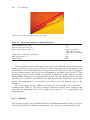
micrograph, shown in Fig. 4.1, was taken at 200 X magnification illuminated with transmitted and polarized light. The microscope was a Leica optical microscope, Laborlux
12 Pol S, equipped with polishing and microtome capability. The illumination could be
transmitted, reflected, and polarized. The micrograph shows that the gel was located
in the middle layer. The discoloration of the material in the middle layer indicated
degradation. At this point the plant was visited and the operation of the extruders was
checked, particularly the 200-mm extruder with L/D = 24.
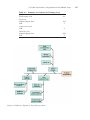
The extruder operating conditions are shown in Table 4.1.