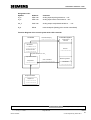
1
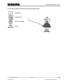
Automation and Drives - SCE
Training Document for Comprehensive Automation
Solutions
Totally Integrated Automation (T I A)
MODULE B3
Control Engineering with STEP 7
T I A Training Document
Issued: 02/2008
Page 1 of 64
Module
B3
Control Engineering with STEP 7
Automation and Drives - SCE
This document has been written by Siemens AG for training purposes for the project entitled "Siemens
Automation Cooperates with Education (SCE)".
Siemens AG accepts no responsibility for the correctness of the contents.
Transmission, use or reproduction of this document is only permitted within public training and educational
facilities. Exceptions require the prior written approval by Siemens AG (Mr. Michael Knust
[email protected]).
Offenders will be liable for damages. All rights, including the right to translate the document, are reserved,
particularly if a patent is granted or utility model is registered.
We would like to thank the following: Michael Dziallas Engineering, the teachers at vocational schools, and all
others who helped to prepare this document.
T I A Training Document
Issued: 02/2008
Page 2 of 64
Module
B3
Control Engineering with STEP 7
Automation and Drives - SCE
Table of Contents
PAGE
1. Preface
2. Fundamentals of Control Engineering
2.2 Components of a Control Loop
2.3. Characteristics
2.4 Step Function for Examining Controlled Systems
2.5. Self-Regulating Processes
2.5.1. Proportional Controlled System without Time Delay
2.5.2. Proportional Controlled System with a Time Delay
2.5.3 Proportional Controlled System with Two Time Delays
2.6 Controlled Systems without Inherent Regulation
2.7 Types of Controllers
2.7.1 Two Position Controllers
2.7.2 Three Position Controllers
2.7.3 Basic Types of Continuous Controllers
2.8 Objectives for Controller Adjustment
2.9 Digital Controllers
3. Discontinuous Action Controller as Two Position Controller
3.1 Function and Problem Description
3.2 Possible Solution for the PLC Program:
4. Controller Block (S)FB41 "CONT_C" as Software PID Controller in STEP 7
4.1 Task Definition for PID Standard Controller
4.2 (S) FB 41 “CONT_C“
4.3 Exercise Example
5. Setting Controlled Systems
5.1 General
5.2 Setting the PI-Controller according to Ziegler-Nichols
5.3 Setting the PID Controller according to Chien, Hrones and Reswick
5.4 Exercise Example
6. Appendix
T I A Training Document
Issued: 02/2008
Page 3 of 64
5
7
8
11
12
13
13
14
15
17
18
18
20
21
27
29
31
31
34
37
37
39
40
54
54
55
55
57
60
Module
B3
Control Engineering with STEP 7
Automation and Drives - SCE
The following symbols provide a guide through this B3 module:
Information
Programming
Exercise Example
Notes
T I A Training Document
Issued: 02/2008
Page 4 of 64
Module
B3
Control Engineering with STEP 7
Automation and Drives - SCE
1. PREFACE
In terms of its contents, Module B3 is part of the teaching unit entitled "Additional Functions of
STEP 7 Programming'.
Basics of
STEP 7 Programming
2 to 3 days
Module A
Additional Functions of
STEP 7 Programming
2 to 3 days Module B
Programming
Languages
2 to 3 days Module C
Industrial
Field Bus Systems
2 to 3 days Module D
Frequency Converter
at SIMATIC S7
2 to 3 days Module H
Plant Simulation with
SIMIT SCE
1 to 2 days Module G
Process
Visualization
2 to 3 days Module F
IT Communication
with SIMATIC S7
2 to 3 days Module E
Learning Objective:
In module B3, the reader learns the following: how a PID controller is integrated into a STEP7
program, how it is wired to analog process variables, and how it is started. The following steps are
discussed:
•
Program example for a two position controller
•
Calling a PID controller in a STEP 7 program
•
Wiring the PID controller to analog process variables
•
Setting the controller parameters at the PID controller
Prerequisites:
To successfully work through Module B3, the following knowledge is assumed:
•
Knowledge in handling Windows
•
Fundamentals of PLC programming with STEP 7 (for example, Module A3 – 'Startup’
PLC Programming with STEP 7)
•
Analog Value Processing with STEP 7 (for example, Module B2 – Analog Value Processing)
Preface
Fundamentals
T I A Training Document
Issued: 02/2008
Discontinuous Action Controllerr
Controller Block (S)FB41
Setting the System
Appendix
Page 5 of 64
Module
B3
Control Engineering with STEP 7
Automation and Drives - SCE
Hardware and software required
1
2
3
4
5
6
PC, operating system Windows 2000 Professional starting with SP4/XP Professional starting
with SP1/Server 2003 with 600MHz and 512RAM, free hard disk storage 650 to 900 MB, MS
Internet Explorer 6.0
Software STEP7 V 5.4
MPI interface for the PC (for example, PC adapter USB)
PLC SIMATIC S7-300 with at least one analog input/output module to which, at one analog
value input, a potentiometer or another analog signal transmitter is connected. In addition, an
analog value display has to be connected to at least one analog output.
Sample configuration:
- Power supply: PS 307 2A
- CPU: CPU 314C-2DP
Controlled System
Connection lines for connecting the controlled system to analog inputs and outputs of the
PLC
2 STEP 7
1 PC
3 PC Adapter USB
6 Connection Lines
4 S7-300 with
CPU 314C-2DP
Preface
Fundamentals
T I A Training Document
Issued: 02/2008
5 Controlled System
Discontinuous Action Controllerr
Controller Block (S)FB41
Setting the System
Appendix
Page 6 of 64
Module
B3
Control Engineering with STEP 7
Automation and Drives - SCE
2. FUNDAMENTALS OF CONTROL ENGINEERING
2.1 Tasks of Control Engineering
"Closed loop control is a process where the value of a variable is established and maintained
continuously through intervention based on measurements of this variable. This creates a sequence
that takes place in a controlled loop -the closed loop- because the process is executed based on
measurements of a variable that is in turn influenced by itself.“
The variable to be controlled is measured continuously and compared with another specified
variable of the same kind. Depending on the result of this comparison, the control process adjusts
the variable to be controlled to the specified variable.
Diagram of a Control System
Comparing
Element
Setpoint
Temperature
Preface
Fundamentals
T I A Training Document
Issued: 02/2008
Controllg.
Element
Actuator
Final Ctrl. Elem.
+ System
Measuring
Device
Discontinuous Action Controller
Controller Block (S)FB41
Setting the System
Appendix
Page 7 of 64
Module
B3
Control Engineering with STEP 7
Automation and Drives - SCE
2.2 Components of a Control Loop
Below, the basic terminology of control engineering is explained in detail.
First, an overview shown in the diagram below:
Controller
Comparing
Element
Controlling
Element
Actuator
Final
Control
Element
Controlled
System
Measuring
Device
1. The Controlled Variable x
It is the actual “objective“ of the control process: the variable that is to be influenced or kept constant
is the purpose of the entire system. In our example, that would be the room temperature. The
momentary value of the controlled variable existing at a certain time is called "actual value“ at that
point in time.
2. The Feedback Variable r
In a control loop, the controlled variable is constantly checked in order to be able to respond to
unintended changes. The measured variable proportional to the controlled variable is called
feedback variable. In the example "furnace“, it would correspond to the measured circuit voltage of
the inside thermometer.
Preface
Fundamentals
T I A Training Document
Issued: 02/2008
Discontinuous Action Controller
Controller Block (S)FB41
Setting the System
Appendix
Page 8 of 64
Module
B3
Control Engineering with STEP 7
Automation and Drives - SCE
4. The Disturbance Variable z
The disturbance variable is the variable that unintentionally influences the controlled variable, and
moves it from the current setpoint value. A fixed setpoint control is necessary, for example, because
a disturbance variable exists. For the heating system considered here, this would be the outside
temperature, for example, or any other variable that changes the room temperature from its ideal
value.
5. The Setpoint Value w
The setpoint value at a point in time is the value that the controlling variable should ideally have at
that time. It should be noted that the setpoint value can change continuously under certain
circumstances if there is a slave value control. The measured value that the measuring device used
would establish if the controlled variable would have exactly the setpoint value is the instantaneous
value of the reference variable. In the example, the setpoint value would be the room temperature
desired at that time.
6. The Comparing Element
This is the point where the current measured value of the controlled variable and the instantaneous
value of the reference variable are compared. In most cases, both variables are measured circuit
voltages. The difference of both variables is the “control deviation“ e. It is passed on to the
controlling element, and evaluated there (see below).
7. The Controlling Element
The controlling element is the actual center piece of a control system. It evaluates the system
deviation -that is, the information about whether, how and to what extent the controlled variable
deviates from the current setpoint- as input information, and derives from this the
“Controller output variable“ YR which, ultimately, influences the controlled variable. The controller
output variable would be, in the example of the heating system, the voltage for the mixer motor.
The manner in which the controlling element determines the controller output variable from the
system deviation is the main criterion of the control system. Part II discusses this topic in greater
detail.
Preface
Fundamentals
T I A Training Document
Issued: 02/2008
Discontinuous Action Controller
Controller Block (S)FB41
Setting the System
Appendix
Page 9 of 64
Module
B3
Control Engineering with STEP 7
Automation and Drives - SCE
8. The Actuator
The actuator is the “executing organ“, so to speak, of the control system. In the form of the controller
output variable, the controlling element provides the actuator with information as to how the
controlled variable is to be influenced, and implements it into a change of the “manipulated variable“.
In our example, the actuator would be the mixer motor. Depending on the voltage supplied by the
controlling element (that is, the controller output variable), it influences the position of the mixer
(which here represents the manipulated variable).
9. The Controlling Element
This is the element of the control loop that influences the controlled variable (more or less directly),
depending on the manipulated variable Y. In the example, this would be the combination consisting
of the mixer, the furnace lines, and the heater. The mixer motor (actuator) sets the mixer (the
manipulated variable). By means of the water temperature, the room temperature is influenced.
10. The Controlled System
The controlled system is the plant where the variable to be controlled is located; in the example of
the radiator, the living space.
11. Dead Time
Dead time refers to the time that passes, starting with a change of the controller output variable until
a measurable reaction by the controlled system. In our example, it would be the time between a
change of the voltage for the mixer motor, and the measurable change in room temperature caused
by this.
Preface
Fundamentals
T I A Training Document
Issued: 02/2008
Discontinuous Action Controller
Controller Block (S)FB41
Setting the System
Appendix
Page 10 of 64
Module
B3
Control Engineering with STEP 7
Automation and Drives - SCE
2.3. Characteristics
Controlled systems in which a new constant output value sets itself after a certain time has passed
are called 'self-regulating process’.
The relationship of the output variables to the input variables in the steady state results in a
characteristic.
Parameter
In the environment of an operating point, the characteristic is replaced with a tangent. In the
environment of an operating point, the problem is treated as a linear problem.
The zero point of the variables x(t), y(t) and z(t) refers to the operating point A:
:
x = X – Xo y = Y - Yo z = Z - Zo
Preface
Fundamentals
T I A Training Document
Issued: 02/2008
Discontinuous Action Controller
Controller Block (S)FB41
Setting the System
Appendix
Page 11 of 64
Module
B3
Control Engineering with STEP 7
Automation and Drives - SCE
2.4 Step Function for Examining Controlled Systems
To examine the behavior of controlled systems, controllers and control loops, a uniform function is
used for the input signal: the step function. Depending on whether a control loop element or the
entire control loop is examined, the step function can be assigned to the following: the controlled
variable x(t), the manipulated variable y(t), the reference variable w(t) or the disturbance variable
z(t). For that reason, the input signal, the step function, is often designated as xe(t), and the output
signal as xa(t).
for
for
Preface
Fundamentals
T I A Training Document
Issued: 02/2008
Discontinuous Action Controller
Controller Block (S)FB41
Setting the System
Appendix
Page 12 of 64
Module
B3
Control Engineering with STEP 7
Automation and Drives - SCE
2.5. Self-Regulating Processes
2.5.1. Proportional Controlled System without Time Delay
The controlled system is called P-system for short.
Abrupt change of the input variable for
Controlled Variable/
Manipulated Variable
Proportional coefficient for a
manipulated variable change
Controlled Variable/
Disturbance Variable
Proportional value for a
disturbance variable change
Range:
Control Range:
Preface
Fundamentals
T I A Training Document
Issued: 02/2008
Discontinuous Action Controller
Controller Block (S)FB41
Setting the System
Appendix
Page 13 of 64
Module
B3
Control Engineering with STEP 7
Automation and Drives - SCE
2.5.2. Proportional Controlled System with a Time Delay
The controlled system is called P-T1 system for short.
Differential equation for a general input signal
Solution of the differential equation for a step function at the input (step response)
Time constant
Preface
Fundamentals
T I A Training Document
Issued: 02/2008
Discontinuous Action Controller
Controller Block (S)FB41
Setting the System
Appendix
Page 14 of 64
Module
B3
Control Engineering with STEP 7
Automation and Drives - SCE
2.5.3 Proportional Controlled System with Two Time Delays
The controlled system is called P-T2 system for short.
Figure: Jump Response of the P-T2 system
Tu: Delay time Tg: Transition time
The system consists of the reaction-free series connection of two P-T1 systems that have the time
constants TS1 and TS2.
Controllability of P-Tn systems:
Can still be
controlled
Easy to
control
Difficult to control
With the rising ratio Tu/Tg, controlling the system becomes more and more difficult.
Preface
Fundamentals
T I A Training Document
Issued: 02/2008
Discontinuous Action Controller
Controller Block (S)FB41
Setting the System
Appendix
Page 15 of 64
Module
B3
Control Engineering with STEP 7
Automation and Drives - SCE
2.5.4 Proportional Controlled System with n Time Delays
The controlled system is called P-Tn system for short.
The time response is described with a differential equation of the nth degree.
The characteristic of the step response is similar to that of the P-T2 system. The time response is
described through Tu and Tg.
Substitute: The controlled system with many delays can be approximately substituted with the series
connection of a P-T1 system with a dead time system.
The following applies: Tt » Tu and TS » Tg.
Substitute step response for the P-Tn system
Preface
Fundamentals
T I A Training Document
Issued: 02/2008
Discontinuous Action Controller
Controller Block (S)FB41
Setting the System
Appendix
Page 16 of 64
Module
B3
Control Engineering with STEP 7
Automation and Drives - SCE
2.6 Controlled Systems without Inherent Regulation
The controlled variable continues to grow after a fault, without aiming for the high range value.
Example: Level Control
In the case of a container with a drain whose inflow volume stream and outflow volume stream are
the same, a constant level is the result. If the flow rate of the inflow or the outflow changes, the liquid
level rises or falls. The larger the difference between inflow and outflow, the faster does the level
change.
The example shows that in practice, the integral action usually has limits. The controlled variable
rises or fills up only so long until it has reached a limit that is contingent on the system: the container
overflows or empties, the pressure reaches the plant maximum or minimum, etc..
The figure shows the trend of an I-system when there is an abrupt change of the input variable, as
well as the block diagram derived from it.
Block Diagram
If the step function at the input changes into any function xe(t), the following happens:
integrating controlled system
integral coefficient of the controlled system
Preface
Fundamentals
T I A Training Document
Issued: 02/2008
Discontinuous Action Controller
Controller Block (S)FB41
Setting the System
Appendix
Page 17 of 64
Module
B3
Control Engineering with STEP 7
Automation and Drives - SCE
2.7 Types of Controllers
2.7.1 Two Position Controllers
The essential feature of two position controllers consists of their knowing only two modes: “On“ and
“Off“ -which makes them the simplest type of controller. Two-position controllers are used primarily
when adhering to a setpoint exactly is less important than to keep the control system as simple as
possible; or, when the actuator or the final control element does not allow for a continuous control
system. The heating system mentioned several times above is -with a control loop having a room
thermometer and a mixer- a continuous control system. To keep the water temperature in the boiler
loop constant, typically a two position controller is used since it can, on the one hand, fluctuate by a
few degrees, and on the other hand it is clearly simpler to switch the burner on and off than to do an
exact dosing of fuel to be added.
Since theoretically -to adhere to the setpoint exactly- it would be necessary to switch a system on
and off infinitely fast, the two position controller has a so-called “hysteresis“. It represents a kind of
“environment“ around the setpoint within which the actual value may fluctuate. That means, we
specify a minimum value that is lower than the setpoint, and a maximum value that is a little higher
than the setpoint. Only if the actual value exceeds the maximum value or drops below the minimum
value does the control system react. In most cases, the minimum and the maximum value are
distanced from the setpoint equally; that is, the hysteresis generates a symmetrical environment
around the set point.
In the case of the boiler water temperature, the burner would be switched on, for example, when the
water temperature drops below the specified setpoint by more than a certain value. The burner
continues to run until a certain value that is above the setpoint is exceeded. Only then will the burner
be switched off. Another typical example is cooling. Usually, a cooler also does not support a
continuous control system, but only knows the states “On“ and “Off“. It is switched on when the
actual temperature exceeds the setpoint temperature by a few degrees, and is switched off when the
actual temperature is a few degrees too low.
It is therefore typical for the two position controller to periodically fluctuate around the setpoint whose
amplitude is roughly that of the hysteresis. The selection of the hysteresis depends on how exactly
the setpoint has to be adhered to. If we select a large hysteresis, the actual value can deviate more
considerably from the setpoint. If we select a smaller one, the setpoint is adhered to more exactly,
but the system would have to switch more frequently. This again has its disadvantages, such as a
higher wear of the switching devices, and the actuator or the final control element.
Preface
Fundamentals
T I A Training Document
Issued: 02/2008
Discontinuous Action Controller
Controller Block (S)FB41
Setting the System
Appendix
Page 18 of 64
Module
B3
Control Engineering with STEP 7
Automation and Drives - SCE
The diagram below shows a two position controller:
Controlled Variable
Switch-Off Value
Hysteresis
Setpoint
Switch-On Value
Manipulated Variable
Time
Time
Preface
Fundamentals
T I A Training Document
Issued: 02/2008
Discontinuous Action Controller
Controller Block (S)FB41
Setting the System
Appendix
Page 19 of 64
Module
B3
Control Engineering with STEP 7
Automation and Drives - SCE
2.7.2 Three Position Controllers
The three position controllers represent the second important class of discrete controllers.
The difference regarding the two position controllers consists in the following: The controller output
can handle three different values: positive influence, no influence, and negative influence of the
controlled variable.
An example is control by means of a valve that can be adjusted electrically but that itself can only be
completely open or completely closed. Let’s take, for example, water level control. As soon as the
water level exceeds a maximum value, the valve motor is triggered with a positive direction of
rotation, and the valve is opened. The control system remains inactive -that is, the motor is idleuntil the water level drops below a minimum value. When this is the case, the motor is triggered into
the negative direction of rotation, and the valve is closed. Thus the actuator knows three states:
rotating valve motor with positive direction of rotation, idle motor, and rotating motor in negative
direction of rotation.
Preface
Fundamentals
T I A Training Document
Issued: 02/2008
Discontinuous Action Controller
Controller Block (S)FB41
Setting the System
Appendix
Page 20 of 64
Module
B3
Control Engineering with STEP 7
Automation and Drives - SCE
2.7.3 Basic Types of Continuous Controllers
The discrete controllers just discussed have, as mentioned before, the advantage of being simple.
The controller itself as well as the actuator and the final control element are of a simpler nature and
thus less expensive than for continuous controllers. However, discrete controllers have a number of
disadvantages. If high loads, such as large electrical motors or cooling systems have to be operated,
high peak loads can occur that can overload the power supply. For these reasons, we often don’t
switch between “Off“ and “On“, but between a full load and a base load -with a clearly lower use of
the actuator or final control element. But even with these improvements, a continuous controller is
not suitable for many applications. Imagine a car engine whose speed is governed discretely. There
would be nothing between idle and full throttle. Aside from it probably being impossible to transfer
the power during a sudden full throttle suitably over the tires onto the road, such a car would
probably be quite unsuitable for street traffic. For such applications, continuous controllers are used
for that reason. Here, the mathematical relationship that the controlling element establishes between
system deviation and controller output variable is theoretically virtually limitless. In practice,
however, we differentiate among three classical basic types that are discussed in greater detail
below.
Preface
Fundamentals
T I A Training Document
Issued: 02/2008
Discontinuous Action Controller
Controller Block (S)FB41
Setting the System
Appendix
Page 21 of 64
Module
B3
Control Engineering with STEP 7
Automation and Drives - SCE
2.7.3.1 Proportional Controllers (P-Controller)
In the case of a P-controller, the controller output y is always proportional to the recorded system
deviation (y ~ e). The result is that a P-controller responds to a system deviation without a delay, and
generates a controller output only if there is a deviation e.
The proportional pressure regulator sketched in the figure below compares the force FS of the
setpoint spring with the force FB that pressure p2 generates on the spring-elastic metal bellows. If
the force is not in balance, the lever rotates around the pivot point D. The valve position
ñ changes, and accordingly the pressure p2 to be controlled until a new power balance is
established. The figure shows the behavior of the P-controller as a sudden system deviation occurs.
The amplitude of the controller output step y depends on the extent of the system deviation e, and
the amount of the proportional coefficient Kp: To keep the system deviation low, a proportional
factor has to be selected that is as large as possible. Increasing the factor accelerates the reaction
of the controller; however, a value that is too high may cause overshoot, and a considerable
oscillatory tendency of the controller.
Metal Bellows
Setpoint Spring
Preface
Fundamentals
T I A Training Document
Issued: 02/2008
Discontinuous Action Controller
Controller Block (S)FB41
Setting the System
Appendix
Page 22 of 64
Module
B3
Control Engineering with STEP 7
Automation and Drives - SCE
The figure below shows the performance of the P-controller:
Controlled
Variable
Setpoint
System
Deviation
Actual
Value
Time
The advantages of this controller type are, on the one hand, its simplicity (the electronic
implementation can, in the simplest case, consist of merely a resistor); on the other hand, in its
prompt reaction in comparison to other controller types. The main disadvantage of a P-controller is
its lasting system deviation. The setpoint is never completely reached, even over long periods of
time. This disadvantage as well as a reaction speed that is not yet ideal can be minimized only
insufficiently by using a larger proportional factor, since otherwise, the controller will overshoot; that
is, it will overreact so to speak. In the worst case, the controller oscillates continuously, whereby the
controlled variable is moved by the controller itself away from the setpoint -instead of by the
disturbance variable.
The problem of continuous system deviation is best solved by the integral action controller.
Preface
Fundamentals
T I A Training Document
Issued: 02/2008
Discontinuous Action Controller
Controller Block (S)FB41
Setting the System
Appendix
Page 23 of 64
Module
B3
Control Engineering with STEP 7
Automation and Drives - SCE
2.7.3.2 Integral Action Controllers (I- Controller)
Integrating controllers are used to completely correct system deviations at every operating point. As
long as the system deviation is not equal to zero, the amount of the controller output changes. Only
when the reference variable and the controlled variable are equal -at the latest however, when the
controller output reaches its system-dependent limit (Umax, Pmax etc.)- is the controller in a steady
state.
The mathematical formula for this integral action is:
The controller output is proportional to the time integral of the system deviation:
with
How fast the controller output rises (or falls), depends on the system deviation and the integration
time.
Block Diagram
Preface
Fundamentals
T I A Training Document
Issued: 02/2008
Discontinuous Action Controller
Controller Block (S)FB41
Setting the System
Appendix
Page 24 of 64
Module
B3
Control Engineering with STEP 7
Automation and Drives - SCE
2.7.3.3 PI Controllers
In practice, the PI controller is a controller type that is used very often. It consists of the parallel
connection of a P-controller and an I-controller. When laid out correctly, it combines the advantages
of both controller types (stable and fast, no lasting system deviation), so that their disadvantages are
compensated for at the same time.
Block Diagram
The trend is indicated with the proportional coefficient Kp and the reset time Tn. Based on the
proportional component, the controller output responds immediately to each system deviation e,
while the integral component has an effect only in the course of time. Tn represents the time that
passes until the I-component generates the same margin of the manipulated variable as it is
generated immediately because of the P-component (Kp). As for the I-controller, the reset time Tn
has to be reduced if you want to increase the integral component.
Controller Layout:
Depending on the Kp and Tn dimensioning, the overshoot of the controlled variable can be reduced
at the expense of control system dynamics.
Applications for the PI controller: fast control loops that don’t permit lasting system deviations.
Examples: pressure, temperature, ratio control.
Preface
Fundamentals
T I A Training Document
Issued: 02/2008
Discontinuous Action Controller
Controller Block (S)FB41
Setting the System
Appendix
Page 25 of 64
Module
B3
Control Engineering with STEP 7
Automation and Drives - SCE
2.7.3.4 Derivative Action Controllers (D-Controller)
The D-controller generates its controller output from the rate of change of the system deviation, and
not -like the P-controller- from its amplitude. For that reason, it still responds considerably faster than
the P-controller. Even if the system deviation is small, it generates -in anticipation, as it were- large
margins of the manipulated variable as soon as the amplitude changes. On the other hand, the Dcontroller does not know a lasting system deviation; because, regardless of how large it is, its rate of
change equals zero. In practice, the D-controller is used rarely by itself for that reason. Rather, it is
used together with other control elements, usually in connection with a proportional component.
2.7.3.5 PID Controllers
If we expand a PI controller with a D-component, we enhance the universal PID controller. As in the
case of the PD controller, adding the D-component has the effect that, if laid out correctly, the
controlled variable reaches its setpoint sooner and enters the steady state faster.
Block Diagram
with
Preface
Fundamentals
T I A Training Document
Issued: 02/2008
Discontinuous Action Controller
Controller Block (S)FB41
Setting the System
Appendix
Page 26 of 64
Module
B3
Control Engineering with STEP 7
Automation and Drives - SCE
2.8 Objectives for Controller Adjustment
For a satisfactory control result, selecting a suitable controller is an important aspect. However,
even more important is the setting of the suitable controller parameters Kp, Tn and Tv that have to
be adjusted to the controlled system behavior. Usually, a compromise has to be made between a
very stable but also slow controller, or a very dynamic, more unstable controlled system
performance, which, under certain circumstances, tends to oscillate and can become unstable.
In the case of non-linear systems that are always to work at the same operational point -for example,
fixed setpoint control- the controller parameters have to be adjusted to the controlled system
behavior at this working point. If, as in the case of cascaded controls ñ, no fixed working point can
be defined, a controller adjustment has to be found which provides a sufficiently fast and stable
control result over the entire work area.
In practice, controllers are usually set based on empirical values. If none are available, the controlled
system behavior has to be analyzed exactly, in order to subsequently specify suitable controller
parameters, with the aid of different theoretical or practical layout procedures.
One possibility of a definition is the oscillation test according to the
Ziegler-Nichols method. It offers a simple layout suitable for many cases. However, this setting
procedure can only be used for controlled systems that permit getting the controlled variable to
oscillate autonomously. The following has to be done:
- Set Kp and Tv at the controller to the lowest value, and Tn to the highest value (the lowest possible
controller effect).
- Take the controlled system manually to the desired operating point (start the controller).
- Set the manipulated variable of the controller manually to the specified value, and switch to the
automatic mode.
- Increase Kp (decrease Xp) until harmonic oscillations can be recognized in the controlled variable.
If possible, the control loop should be stimulated to oscillate during the Kp setting by using small,
abrupt setpoint changes.
Preface
Fundamentals
T I A Training Document
Issued: 02/2008
Discontinuous Action Controller
Controller Block (S)FB41
Setting the System
Appendix
Page 27 of 64
Module
B3
Control Engineering with STEP 7
Automation and Drives - SCE
- Note down the Kp value that has been set as the critical proportional coefficient.
- Specify the duration of a complete oscillation as Tkrit, perhaps with a stop watch by generating the
arithmetical mean over several oscillations.
- Multiply the values of Kp,krit and Tkrit with the multipliers according to the table, and thus set the
determined values for Kp, Tn and Tv at the controller.
0.50
Preface
Fundamentals
T I A Training Document
Issued: 02/2008
0.45
0.85
0.59
0.50
Discontinuous Action Controller
Controller Block (S)FB41
0.12
Setting the System
Appendix
Page 28 of 64
Module
B3
Control Engineering with STEP 7
Automation and Drives - SCE
2.9 Digital Controllers
So far, mainly analog controllers were discussed; that is, such controllers that derive the controller
output variable -also in an analog way- from the existing system deviation that exists as analog
value. We are already familiar with the diagram of such a control loop:
Comparing
Element
Analog
Controller
System
Often, however, it has its advantages to evaluate the system deviation digitally. On the one hand,
the relationship between system deviation and controller output variable has to be specified much
more flexibly if it is defined through an algorithm or a formula with which a computer can be
programmed respectively, as when it has to be implemented with an analog circuit. On the other
hand, a clearly higher integration of circuits is possible in digital engineering, so that several
controllers can be accommodated in the smallest space. And finally, by dividing the computing time it
is even possible -if the computing capacity is sufficiently large- to use a single computer as
controlling elements of several control loops.
To make digital processing of the variables possible, the reference variable as well as the feedback
variable have to first be converted in an analog-digital converter (ADC) into digital variables. These
are then subtracted from each other by a digital comparing element, and the difference is transferred
to the digital controlling element. Its controller output variable is then converted again in a digitalanalog converter (DAC) into an analog variable. The unit consisting of converters, comparing
element, and controlling element appears to the outside like an analog controller.
Preface
Fundamentals
T I A Training Document
Issued: 02/2008
Discontinuous Action Controller
Controller Block (S)FB41
Setting the System
Appendix
Page 29 of 64
Module
B3
Control Engineering with STEP 7
Automation and Drives - SCE
The diagram below shows the layout of a digital controller:
Comparing
Element
Digital
Controller
DAC
System
ADC
However, the digital conversion of the controller has not only advantages; this conversion also
entails various problems. For that reason, some variables have to be selected sufficiently large in
reference to the digital controller so that the accuracy of the control does not suffer too much on
account of digitalization. Quality criteria for digital computers are:
•
The quantization resolution of the digital-analog converters.
It indicates how fine the continuous value range is digitally rasterized. The resolution has to be
selected of a size that no resolutions important to the controller are lost. .
•
The scanning frequency of the analog-digital converters.
This is the frequency with which the analog values pending at the converter are measured and
digitalized. This has to be high enough that the controller can still respond in time if the controlled
variable suddenly changes.
•
The cycle time
In clock cycles, every digital computer processes differently than the analog computer. The speed of
the computer used has to be high enough that during a clock cycle (during which the output value is
calculated, and no input value is scanned), the controlled variable can not change significantly.
The quality of the digital controller has to be high enough so that toward the outside, it responds
comparably prompt and precise, like an analog controller does.
Preface
Fundamentals
T I A Training Document
Issued: 02/2008
Discontinuous Action Controller
Controller Block (S)FB41
Setting the System
Appendix
Page 30 of 64
Module
B3
Control Engineering with STEP 7
Automation and Drives - SCE
3. DISCONTINUOUS ACTION CONTROLLER AS TWO POSITION CONTROLLER
3.1 Function and Problem Description
A process value (for example, the level) is to be kept as constant as possible with a discontinuous
action controller.
The output voltage at a digital output of the PLC generates the manipulated variable y which can be
set either to "ON" (voltage =24V) or "OFF" (voltage =0V).
The process value represents the controlled variable x, which is suitably recorded with a measuring
sensor (PEW XY).
It is the controller’s task to keep the controlled variable X constant at a specified setpoint, whereby
the influence of disturbance variables z that can not be anticipated is to be eliminated. The PLC S7300 is used for this task as discontinuous action controller. The S7-300 is to solve the control
problem by reading out a binary manipulated variable y depending on the respective setpoint/actual
comparison w-x.
To prevent valve V1 from constantly being switched on and off when the controlled variable x has
reached the setpoint w, a switching hysteresis is installed for discontinuous action controllers.
Because of the switching hysteresis, the controlled variable x oscillates between a high response
value Xo and a low response value Xu. The difference between the high response value Xo and the
low response value Xu is called differential Xs = Xo - Xu.
Xs is often specified depending on the amount of setpoint w.
For example, 10% of setpoint w: Xs = w/10.
In this program, a two position controller can be switched on with the button “Start“ to fill a tank.
With the button “Stop“, the controller can be switched off. The tank is filled by means of a pump that
can be triggered digitally. The setpoint is specified via a potentiometer at the analog input
"AI_Fill_Setpoint“.
In a subroutine, the analog value for the process variable Level is to be entered, and normalized to
the physical variable "Liter“. The normalized value is made available as floating point number in
MD20.
For a level of 10 liters, the level sensor returns 0V, for 100 liters 10V.
The analog value for the setpoint is also to be entered here, and made available as floating point
number in MD24.
If the controller is switched on, the lamp "Display_ON“ is to light up.
Below, the structogram for the program of the step controller is provided.
Preface
Fundamentals
T I A Training Document
Issued: 02/2008
Discontinuous Action Controllerr
Controller Block (S)FB41
Setting the System
Appendix
Page 31 of 64
Module
B3
Control Engineering with STEP 7
Automation and Drives - SCE
Structogram
A structogram shows the rough structure of a program plan. The structogram below shows the
possible structure of a program for a two position controller.
First, a scan is made whether the controller is switched on.
If it is switched off, only the program is executed in which the outputs and flags are reset.
From the program-engineering view, this is done most simply by means of jump instructions.
If the controller is switched on, the setpoint and actual value are entered, and the calculations for
switching hysteresis, differential and the lower operating point are made.
Then, another scan follows: whether the actual value is below the low operating point.
If this is the case, the controller output is switched on, and a jump is made to the end of the program.
If this is not the case, the high operating point is calculated, and a scan is made whether the actual
value is above the high operating point.
Then, again a jump is made to the end of the program.
Controller switched off?
YES
NO
Outputs
Display: Switch on SH10
and
Enter actual value x and
Flags
setpoint w
Normalize
Clear
Calculation of the switching hysteresis Xs = w/10
or
Calculation of half the differential X1 = Xs/2
Reset
Calculation of the low operating point Xu = w - X1
Is the actual value less than the low operating point?
YES
NO
Pump ON
Calculation of the high operating point Xo = w + X1
Actual value X larger than Xo?
YES
NO
Pump OFF
Preface
Fundamentals
T I A Training Document
Issued: 02/2008
Discontinuous Action Controllerr
Controller Block (S)FB41
Setting the System
Appendix
Page 32 of 64
Module
B3
Control Engineering with STEP 7
Automation and Drives - SCE
Assignment List:
Symbol:
Start
Stop
Address:
I
1.3
I
1.4
Comment
Button Start
Button Stop
AI_Level_Actual
AI_Level_Setpoint
PEW 128
PEW 130
Analog input for the level sensor
Analog input for the setpoint selection
AI_Level_Act_Norm MD 20
AI_Level_Setp_Norm MD 24
M_X1
MD 32
M_Xo
MD 36
M_Xs
MD 28
M_Xu
MD 40
Controller_On
M
10.0
Normalized value for the level
Normalized value for the level setpoint
Intermediate flag half the differential
Intermediate flag high operating point
Intermediate flag switching hysteresis
Intermediate flag low operating point
Flag controller is switched on
Pump
Display_ON
Pump activation binary
Indication: system is on
A
A
Analog
FC1
Two Pos.Controller FC2
0.0
1.0
Subroutine analog value processing
Subroutine two position controller
Exercise:
Create a project with hardware configuration for a CPU314C-2 DP (refer to Module A05) and change
the addresses according to the assignment list shown above.
There, create a program in an FC1 with the following functionality:
- The analog value for the process variable Level is to be entered, and normalized to the physical
variable "Liter“. The normalized value is made available in MD20 as a floating point number.
Note: If the level is 10 liters, the level sensor returns 0V, for 100 liters 10V.
- The analog value for the setpoint is to be entered, and made available normalized as floating point
number in MD24.
Save FC1.
Then, set up the two position controller in an FC2, based on the structogram provided above.
Call FC1 for inputting the setpoint and the actual value.
Save FC2 and call it in OB1. Save OB1 and load the entire station to the PLC.
Preface
Fundamentals
T I A Training Document
Issued: 02/2008
Discontinuous Action Controllerr
Controller Block (S)FB41
Setting the System
Appendix
Page 33 of 64
Module
B3
Control Engineering with STEP 7
Automation and Drives - SCE
3.2 Possible Solution for the PLC Program:
Analog Value Processing
Network 1:
Enter and normalize analog value of actual level
"AI_Level_Actual“
"AI_Level_Actual_Norm“
Network 2:
t i t L
Enter and normalize analog value of setpoint level
l
"AI_Level_Setp“
"AI_Level_Setp_Norm“
****************************************************************************************************************
Two Position Contoller
Network 1: Controller switched on?? If off, then jump to label "Off“
"Start“
"Controller_On“
"Stop“
"Controller_On“
"Controller_On“
"Ind_ON“
exit
Network 2: Call subroutine: enter and normalize analog values
Network 3: Calculation of switching hysteresis Xs = w/10
"AI_Fill_Setp_Norm“
Preface
Fundamentals
T I A Training Document
Issued: 02/2008
Discontinuous Action Controllerr
Controller Block (S)FB41
Setting the System
Appendix
Page 34 of 64
Module
B3
Control Engineering with STEP 7
Automation and Drives - SCE
Network 4:
Calculation of half differential X1 = Xs/2
Network 5:
Calculation of the low operating point Xu = w – X1
"AI_Fill_Setp_Norm“
Network 6:
ACTUAL VALUE x less than low operating point?
D24/AI_Fill_Setp_Norm/Norm.value for level setpoint
"AI_Fill_Actual_Norm“
"Pump“
Network 7:
Calculation of the high operating point Xo = w – X1
"AI_Fill_Setp_Norm“
Network 8:
Actual value X larger than Xo?
"AI_Level_Actual_Norm“
"Pump“
Preface
Fundamentals
T I A Training Document
Issued: 02/2008
Discontinuous Action Controllerr
Controller Block (S)FB41
Setting the System
Appendix
Page 35 of 64
Module
B3
Control Engineering with STEP 7
Automation and Drives - SCE
Network 9:
Reset values
exit:
"AI_Fill_Actual_Norm“
"AI_Fill_Setp_Norm
"Pump“
"Pump“
"Display_ON“
"Display_ON“
Network 10:
Title
****************************************************************************************************************
OB1:
Title
Network 1:
Call subroutine: Two position controller
"Two Position
Controller“
Preface
Fundamentals
T I A Training Document
Issued: 02/2008
Discontinuous Action Controllerr
Controller Block (S)FB41
Setting the System
Appendix
Page 36 of 64
Module
B3
Control Engineering with STEP 7
Automation and Drives - SCE
4. CONTROLLER BLOCK (S)FB41 "CONT_C" AS SOFTWARE PID CONTROLLER IN STEP 7
4.1 Task Definition for PID Standard Controller
In this B3 module, the startup of a PID controller in SIMATIC S7 is demonstrated. The output value
of the controlled system is to be kept constant with a continuous controller. Depending on the
setting, the controlled system can simulate a P, PT1, or PT2 system. The transfer coefficients Ks
and the time constants can also be set. (refer to the description of the controlled system).
Thus, the PLC is the controller, and is connected to the controlled system by means of analog inputs
and outputs.
The block (S)FB 41 in the PLC SIMATIC S7-300 is used in this task as a continuous digital software
controller. It is to solve the control problem as follows: an analog manipulated variable y is read out
depending on the respective setpoint/actual value w-x. The manipulated variable y is generated
according to the PID algorithm.
The following control parameters can be specified:
KP: Proportional component (for (S)FB41 Gain)
TN: Integrator time (for (S)FB41 TI)
TV: Derivative time (for (S)FB41 TD)
Preface
Fundamentals
T I A Training Document
Issued: 02/2008
Discontinuous Action Controllerr
Controller Block (S)FB41
Setting the System
Appendix
Page 37 of 64
Module
B3
Control Engineering with STEP 7
Automation and Drives - SCE
Assignment List:
Symbol:
AI_w
AI_X
Address:
PEW 128
PEW 130
Comment
Analog input setpoint generator 0…10V
Analog input sensor actual value 0…10V
AO_Y
PAW 128
Analog output manipulated variable 0 … 10V
M_w
MD40
Internal setpoint (floating point number normalized)
Function Diagram of the control system with a PID controller
Controller
Regler
Controller Output y
Stellgröße y
Regelstrecke
Controlled
System
Final Control
Stellglied
Element
Generation
Bildung
of
der
Process
Prozess
Control
Function
Regelfunktion
System
Deviatione e==w-x
w-x
Regeldifferenz
Setp./Actual
Value
Soll-IstwertComparison
Vergleich
Contr.
Variablexx
Regelgröße
Measuring
Sensor
Messgeber
Transducer
Messumformer
Setpoint Generator
Sollwertgeber
Setpoint
SollwertInt
Int
Preface
Fundamentals
T I A Training Document
Issued: 02/2008
Discontinuous Action Controllerr
Controller Block (S)FB41
Setting the System
Appendix
Page 38 of 64
Module
B3
Control Engineering with STEP 7
Automation and Drives - SCE
4.2 (S) FB 41 “CONT_C“
(S)FB 41 "CONT_C“ (continuous controller) is used for controlling technical processes with
continuous input and output variables on the PLC SIMATIC S7. By means of parameter
assignments, you can switch on or switch off subfunctions of the PID controller, and thus adjust it to
the controlled system.
Use:
You can use the controller as PID fixed setpoint controller individually, or in multi-loop control
systems as cascade controller, blended controller, or ratio controller. The working method is based
on the PID algorithm of the sampling controller with analog output signal; if needed, supplemented
with a pulse shaper step to generate pulse-width-modulated output signals for two position or three
position controller with proportional final control elements.
Description:
In addition to the functions in the setpoint and actual value, the (S)FB implements a complete PID
controller with a continuous manipulated variable output and the capability to influence the
manipulated value manually.
Depending on the CPU type, it can be used as FB 41 or as SFB 41.
The following subfunctions exist:
-
Setpoint branch
Actual value branch
System deviation generation
PID algorithm
Manual value processing
Manipulated value processing
Feedforward control
Operating modes complete restart/restart
The (S)FB 41 (CONT_C) has a complete restart routine that is run if the input parameter is set to
COM_RST = TRUE.
At startup, the integrator is set internally to the initialization value I_ITVAL. When called in a time
interrupt level, it continues processing starting with this value.
The other outputs are set to their default values.
Error Information
The error signal word RET_VAL is not used.
Preface
Fundamentals
T I A Training Document
Issued: 02/2008
Discontinuous Action Controllerr
Controller Block (S)FB41
Setting the System
Appendix
Page 39 of 64
Module
B3
Control Engineering with STEP 7
Automation and Drives - SCE
Starting Up the Software PID Controller (S)FB41 "CONT_C" with STEP 7
A SIMATIC S7-300 is programmed as a PID controller with the software STEP 7. This provides the
user with a uniform configuring tool for central as well as distributed configurations. Here, only the
most essential aspects can be pointed out. (Additional information is provided in the STEP7
reference manuals.)
The PID controller is parameterized with a special application included in STEP7 -Assigning
parameters to a PID Control- by resetting values there in an instance DB associated with the (S)FB
41. This is done as follows:
4.3 Exercise Example
The user has to perform the steps below in order to configure the hardware as well as to generate an
S7 program with the functionality of a PID controller, and then load it to a PLC:
1.
Call the SIMATIC Manager
Click on symbol
'SIMATIC Manager’
2.
Set up new project ( → File → New)
Click on 'New'
Preface
Fundamentals
T I A Training Document
Issued: 02/2008
Discontinuous Action Controllerr
Controller Block (S)FB41
Setting the System
Appendix
Page 40 of 64
Module
B3
Control Engineering with STEP 7
Automation and Drives - SCE
3. Generate a new project, select a path and assign a project name (→ User projects →
PID_Control → OK)
Select 'User
Projects’
Enter project
name
Select storage
location (path)
Cick 'OK'
4.
Insert the SIMATIC 300 station (→ Insert → Station → SIMATIC 300 Station)
Click on 'SIMATIC 300
Station'
Preface
Fundamentals
T I A Training Document
Issued: 02/2008
Discontinuous Action Controllerr
Controller Block (S)FB41
Setting the System
Appendix
Page 41 of 64
Module
B3
Control Engineering with STEP 7
Automation and Drives - SCE
5.
Highlight 'SIMATIC 300 Station(1)’.
Click on
'SIMATIC 300
Station(1)'
6.
Open configuring tool for the hardware configuration (→ Edit → Open object)
Click on 'Open
object’
Preface
Fundamentals
T I A Training Document
Issued: 02/2008
Discontinuous Action Controllerr
Controller Block (S)FB41
Setting the System
Appendix
Page 42 of 64
Module
B3
Control Engineering with STEP 7
Automation and Drives - SCE
7.
Open the hardware catalog.
Here, all racks, modules, and interface modules for configuring your hardware, are provided
arranged in the directories: PROFIBUS-DP, SIMATIC 300, SIMATIC 400 and SIMATIC PC
Based Control.
Click on the
symbol for 'HW
catalog’
8.
Insert mounting channel (→ SIMATIC 300 → RACK-300 → Mounting channel).
Click on 'Mounting
channel'
Then a configuration table is displayed automatically for configuring Rack 0.
Preface
Fundamentals
T I A Training Document
Issued: 02/2008
Discontinuous Action Controllerr
Controller Block (S)FB41
Setting the System
Appendix
Page 43 of 64
Module
B3
Control Engineering with STEP 7
Automation and Drives - SCE
9.
From the hardware catalog, all modules that are plugged inserted in your real rack can now be
selected and inserted in the configuration table. To this end, you have to click on the name of
the respective module, hold the mouse key and drag the module to a line in the configuration
table.
Note: Slot 3 is reserved for interface modules, and remains empty for that reason.
Preface
Fundamentals
T I A Training Document
Issued: 02/2008
Discontinuous Action Controllerr
Controller Block (S)FB41
Setting the System
Appendix
Page 44 of 64
Module
B3
Control Engineering with STEP 7
Automation and Drives - SCE
10. Note down the addresses of the IO modules (addresses are assigned automatically and
tied to the slot).
For our example, change the addresses to the values PEW 128 and PAW 128.
Save the configuration table and load it to the PLC (key switch on CPU has to be on Stop!)
Click on symbol ‘Load to
AS’
Click on symbol ‘Save and
convert’
Double click on line "AI5/A02,
then re-write start addresses to
PEW/PAW 128
11. Highlight Blocks in SIMATIC Manager
Click on 'Blocks'
Preface
Fundamentals
T I A Training Document
Issued: 02/2008
Discontinuous Action Controllerr
Controller Block (S)FB41
Setting the System
Appendix
Page 45 of 64
Module
B3
Control Engineering with STEP 7
Automation and Drives - SCE
12. Insert organization block. (→ Insert → S7 Block → Organization block)
Click on 'Organization
block’
13. Assign OB35 as name of block.( → OB35 → OK)
Note:
Preface
Fundamentals
T I A Training Document
Issued: 02/2008
OB35 is a so-called 'Time interrupt OB’ and ensures a
constant cycle for calling the PID controller block SFB41.
This is absolutely necessary so that the controller can be optimized by
setting the controller parameters KP, TN and TV (for (S)FB41 Gain, TI and TD).
A cycle that under certain circumstances would fluctuate -as in the case of OB1- would
cause the controlled system to fluctuate, and in the worst case, we would have a
controlled variable that would be oscillating in an unstable way.
Discontinuous Action Controllerr
Controller Block (S)FB41
Setting the System
Appendix
Page 46 of 64
Module
B3
Control Engineering with STEP 7
Automation and Drives - SCE
14. In the hardware configuration, at Properties of the CPU, a fixed cycle time can be set for
executing OB35.
However, this cycle time should not be selected too short. It has to be ensured that all blocks
called from OB35 can be processed within this time, and if OB1 is used at the same time, that
there is enough time for it also. (→ Execution)
Enter execution
time
15. Open ‘OB35’ from SIMATIC Manager (→ OB35)
Double click on block
'OB35'
Preface
Fundamentals
T I A Training Document
Issued: 02/2008
Discontinuous Action Controllerr
Controller Block (S)FB41
Setting the System
Appendix
Page 47 of 64
Module
B3
Control Engineering with STEP 7
Automation and Drives - SCE
16. With ‘LAD, STL, and FBD – Program S7 Blocks’, you now have an editor that allows you to
edit your STEP7 program accordingly. To this end, OB35 has already been opened with the
first network.
To generate your first operations, you have to highlight the first network. Now you can write your
fist STEP7 program.
In STEP 7, individual programs are usually subdivided into networks. You open a new network
by clicking on the network symbol.
Note: Comments on program documentation are separated from the program commands by the
character sequence“//“.
Open new
network
Highlight network and write
program
The network
Call SFB41,DB41
calls the PID controller block SFB41 together with an instance DB.
Generate instance DB (→ Yes)
Preface
Fundamentals
T I A Training Document
Issued: 02/2008
Discontinuous Action Controllerr
Controller Block (S)FB41
Setting the System
Appendix
Page 48 of 64
Module
B3
Control Engineering with STEP 7
Automation and Drives - SCE
17. The setpoint value, the actual value and the manipulated variable now have to be wired to
process values as follows.
Cycle time:
Time between the block
call. Should correspond
to the time that is set in
OB 35.
SP INT:
Setpoint selection through analog input.
Has to be normalized to a real format
(refer to NW 2)
PV PER
Actual value
acceptance to
analog input
channel
LMN PER:
Manipulated variable
output at analog
output
Preface
Fundamentals
T I A Training Document
Issued: 02/2008
Discontinuous Action Controllerr
Controller Block (S)FB41
Setting the System
Appendix
Page 49 of 64
Module
B3
Control Engineering with STEP 7
Automation and Drives - SCE
18. Save and load OB35 (CPU’s key switch is on Stop!)
19. In ‘SIMATIC Manager’, highlight block DB41 and load to the PLC. (CPU’s key switch is on
Stop!)
Click on symbol ‘Load to
PLC’
Click on DB41
Preface
Fundamentals
T I A Training Document
Issued: 02/2008
Discontinuous Action Controllerr
Controller Block (S)FB41
Setting the System
Appendix
Page 50 of 64
Module
B3
Control Engineering with STEP 7
Automation and Drives - SCE
20. Call the tool Assign parameters to the PID control (→ Start → Simatic → STEP 7 →
Parameterize PID Control)
Click on ‘Parameterize PID
Control’
Preface
Fundamentals
T I A Training Document
Issued: 02/2008
Discontinuous Action Controllerr
Controller Block (S)FB41
Setting the System
Appendix
Page 51 of 64
Module
B3
Control Engineering with STEP 7
Automation and Drives - SCE
21. Open data block ( → File → Open → Online
→ Select data block; for example, DB41 → OK).
Click on ‘Open’
Switch block to the online
mode
DB 41 auswählen
Click on ‘OK’
Preface
Fundamentals
T I A Training Document
Issued: 02/2008
Discontinuous Action Controllerr
Controller Block (S)FB41
Setting the System
Appendix
Page 52 of 64
Module
B3
Control Engineering with STEP 7
Automation and Drives - SCE
22.
The PID controller can now be parameterized with the tool Parameterize PID Control.
Then, the DB is saved (→ Save) and loaded to the PLC (→ Load).
Now, a curve plotter can be started in order to monitor the performance of the
controlled system.
Click on ‘Save’
Click on ‘Load’
Start ‘Curve plotter’
23. With the curve plotter, the curves for setpoint, actual value and manipulated variable can be
recorded.
24. The program is started by setting the key switch to RUN.
Preface
Fundamentals
T I A Training Document
Issued: 02/2008
Discontinuous Action Controllerr
Controller Block (S)FB41
Setting the System
Appendix
Page 53 of 64
Module
B3
Control Engineering with STEP 7
Automation and Drives - SCE
5. SETTING CONTROLLED SYSTEMS
5.1 General
Below, setting controlled systems is discussed, using a PT2 system as an example.
Tu-Tg Approximation
The basis for the methods according to Ziegler-Nichols and according to Chien, Hrones and
Reswick is the Tu-Tg approximation. With it, the parameters following parameters transfer coefficient
of the system KS, delay Tu und transition time Tg can be determined from the system step response.
The rules for controller adjustment that are described below were found experimentally, by using
analog computer simulations.
P-TN systems can be described with sufficient accuracy with a so-called Tu-Tg approximation; that
means, through approximation by means of a P-T1-TL system.
Starting point is the system step response with the input step height K. The necessary parameters:
transfer coefficient of the system KS, delay Tu and transition time Tg are ascertained as shown in the
figure below.
This requires measuring the transition function up to the stationary upper range value (K*Ks), so that
the transfer coefficient for system KS, required for the calculation, can be determined.
The essential advantage of these methods is that the approximation can also be used if the system
can not be described analytically.
x/%
K*KS
Turning
Point
Wendepunkt
Tu
Figure:
Preface
Issued: 02/2008
t/sec
Tu-Tg Approximation
Fundamentals
T I A Training Document
Tg
Discontinuous Action Controller
Controller Block (S)FB41
Setting the System
Appendix
Page 54 of 64
Module
B3
Control Engineering with STEP 7
Automation and Drives - SCE
5.2 Setting the PI-Controller according to Ziegler-Nichols
By experimenting with P-T1-TL systems, Ziegler and Nichols have found the following optimum
controller settings for fixed setpoint control:
Tg
KPR =0.9
0,9
K ST u
TN = 3.3
3,33 Tu
In general, we get disturbance characteristics with these setting values that are quite good. [7]
5.3 Setting the PID Controller according to Chien, Hrones and Reswick
For this method, the response to setpoint characteristics as well as disturbance characteristics was
examined, in order to get the most favorable controller parameters. Different values resulted for
both cases.
The following settings were the result:
• For disturbance characteristics:
aperiodischer
EinschwingApriodical
transient
reaction
vorgang
mit kürzester
with
the shortest
period Dauer
20%
overshoot
20%
Überschwingen
Minimum
period
of oscillation r
minimale
Schwingungsdaue
Tg
KPR = 0.6
0,6
Tg
KPR = 0,7
0.7
KSTu
K ST u
TN = 2.3
2,3 Tu
TN = 4 T u
Preface
Fundamentals
T I A Training Document
Issued: 02/2008
Discontinuous Action Controller
Controller Block (S)FB41
Setting the System
Appendix
Page 55 of 64
Module
B3
Control Engineering with STEP 7
Automation and Drives - SCE
• For setpoint characteristic:
aperiodischer
Einschwing
Apriodical
transient
reaction mit kürzeste
withvorgang
the shortest
period r Dauer
20%
overshoot
20%
Überschwingen
Minimum
period
of oscillation r
minimale
Schwingungsdaue
Tg
0.35
KPR = 0,35
KPR = 0.6
0,6
K ST u
KSTu
TN = 1.2
1,2 Tg
Preface
Fundamentals
T I A Training Document
Issued: 02/2008
Tg
TN = Tg
Discontinuous Action Controller
Controller Block (S)FB41
Setting the System
Appendix
Page 56 of 64
Module
B3
Control Engineering with STEP 7
Automation and Drives - SCE
5.4 Exercise Example
To accommodate the system step response, a few modifications have to be made in OB 35 and
DB41. The following steps have to be performed for this:
Save your old project under a new name, and change the wiring of (S)FB 41 as follows:
1. With STEP7, specify the manipulated value directly.
The manipulated value is to be specified in the network below in a way that with a switch
S1 (I 124.0), a selection can be made between two manipulated values.
M001:
L
0.000000e+000
//Manipulated value 0% as 32 bit floating point number
UN
I 124.0
//Negation of S1 (I 124.0)
SPB
M001
//Jump if RLO = 1 to label M001
L
1.000000e+002
//Manip.value 100% as 32 bit floating pt. nbr.
T
MD 20
//Transfer the value to flag double word MD 20
Now, for the switch position S1(I 124.0) ON, the manipulated variable y = 100%, and for OFF, the
manipulated variable y = 0%. Consequently, a step of the manipulated value from 0 to 100% can be
brought about with Switch S1. (For systems that tend to overshoot, the high manipulated value
should amount to 90% or less.).
The external analog values and the manipulated value are assigned in OB1 as follows:
MAN
:=
MD 20
//Specify the manipulated value as manual value
PV_PER
:=
PEW 130
//Actual value x
LMN_PER
:=
PAW 128
//Manipulated variable y
Switch manipulated value to manual
mode
Preface
Fundamentals
T I A Training Document
Issued: 02/2008
Discontinuous Action Controller
Controller Block (S)FB41
Setting the System
Appendix
Page 57 of 64
Module
B3
Control Engineering with STEP 7
Automation and Drives - SCE
Solution of the PLC program:
Network 1: Call
PID Controller
Wiring the manual value to thevalue 0 or
100% of the manipulated value
(Refer to NW 2 and NW 3)
Preface
Network 2:
Default Manipulated value 100%
Network 3:
Default Manipulated value 0%
Fundamentals
T I A Training Document
Issued: 02/2008
Discontinuous Action Controller
Controller Block (S)FB41
Setting the System
Appendix
Page 58 of 64
Module
B3
Control Engineering with STEP 7
Automation and Drives - SCE
Then, the system step response is recorded with the curve plotter from 0 to 100%.
For systems that tend to overshoot, 90% should be assigned as step value.
Setpoint
Turning Point
Tu
Tg
System step response for Tu-Tg approximation
After the inflectional tangent is drawn in the figure, the following values can be read:
Tu = 0.7s
Tg = 7s
1.0 * KS = 1.0
The result is KS = 1.0 and the ratio Tg/KS = 7s.
Setting the PI controller according to Ziegler-Nichols
The following controller parameters result with the values Tu-Tg approximation, and the rules for
controller adjustment according to Ziegler-Nichols:
KPR = 9
TN = 2.3s
These controller parameters are transferred to DB41.
Preface
Fundamentals
T I A Training Document
Issued: 02/2008
Discontinuous Action Controller
Controller Block (S)FB41
Setting the System
Appendix
Page 59 of 64
Module
B3
Control Engineering with STEP 7
Automation and Drives - SCE
6. APPENDIX
Diagram of the controller block:
Preface
Fundamentals
T I A Training Document
Issued: 02/2008
Discontinuous Action Controller
Controller Block (S)FB41
Setting the System
Appendix
Page 60 of 64
Module
B3
Control Engineering with STEP 7
Automation and Drives - SCE
Input Parameters
Parameter
Preface
Value Range
Default
Description
COM_RST
BOOL
FALSE
COMPLETE RESTART. The block has a
complete restart routine that is processed if the
input is set to "Complete restart".
MAN_ON
BOOL
TRUE
MANUAL VALUE ON / Switch on manual
operation. If the input "switch on manual
operation" is set, the control loop has been
interrupted. A manipulated value is entered as
manual value.
PVPER_ON
BOOL
FALSE
PROCESS VARIABLE PERIPHERY ON /
Actual value
Switch on the periphery. If the periphery is to
read in the actual value, input PV_PER has to
be wired to the periphery, and the input "Switch
on actual value periphery" has to be set.
P_SEL
BOOL
TRUE
PROPORTIONAL ACTION ON / Switch on Pcomponent. In the PID algorithm, the PID
components can be switched on/off individually.
The P-component is switched on if the input
"Switch on P-component" is set.
I_SEL
BOOL
TRUE
INTEGRAL ACTION ON / Switch on Icomponent. In the PID algorithm, the PID
components can be switched on/off individually.
The I-component is switched on if the input
"Switch on I- component" is set.
INT_HOLD
BOOL
FALSE
INTEGRAL ACTION HOLD / Freeze Icomponent. The output of the integrator can be
frozen. To this end, the input "Freeze Icomponent“ is set.
I_ITL_ON
BOOL
FALSE
INITIALIZATION OF THE INTEGRAL ACTION /
Set I-component. The output of the integrator
can be set to the input I_ITL_VAL. To this end,
the input "Set I-component“ has to be set.
D_SEL
BOOL
FALSE
DERIVATIVE ACTION ON / Switch on Dcomponent. In the PID algorithm, the PID
components can be switched on/off individually.
The D-component is switched on if the input
"Switch on D-component" is set.
Fundamentals
T I A Training Document
Issued: 02/2008
Data
Type
Discontinuous Action Controller
Controller Block (S)FB41
Setting the System
Appendix
Page 61 of 64
Module
B3
Control Engineering with STEP 7
Automation and Drives - SCE
Parameter
Preface
Default
Description
CYCLE
TIME
>= 1 ms
T#1s
SP_INT
REAL
-100.0...+100.0%
0.0
INTERNAL SETPOINT. The input "Internal
setpoint" is used to specify the setpoint.
PV_IN
REAL
-100.0...+100.0%
0.0
PROCESS VARIABLE IN / Actual value input.
At the input "Actual value input", a startup
value can be parameterized, or an external
actual value can be wired in the floating point
format.
PV_PER
WORD
MAN
REAL
GAIN
REAL
TI
TIME
>= CYCLE
T#20s
RESET TIME / Integration time. The input
"Integration time" determines the time
response of the integrator.
TD
TIME
>= CYCLE
T#10s
TM_LAG
TIME
>=CYCLE/2
T#2s
DEADB_W
REAL
>=0.0 %
0.0
DERIVATIVE TIME. The input "Derivative
time" determines the time response of the
differentiator.
TIME LAG OF THE DERIVATE ACTION /
Delay of the D-component. The algorithm of
the D-component contains a delay that can be
parameterized at the input "Time lag of the
derivative action".
DEAD BAND WIDTH. The system deviation
is taken via a dead band. The "Dead band
width" determines the size of the dead band.
Fundamentals
T I A Training Document
Issued: 02/2008
Data Type Value Range
W#16#0000
-100.0...+100.0%
Discontinuous Action Controller
SAMPLE TIME. The time between block calls
has to be constant. The input "Sample time"
indicates the time between block calls.
PROCESS VARIABLE PERIPHERy / Actual
value Periphery. The actual value in the
periphery format is wired to the controller at
the input "Actual value Periphery ".
0.0
MANUAL VALUE. The input "Manual value" is
used to specify a manual value by means of
the operator interface function.
2.0
PROPORTIONAL GAIN /Proportional
coefficient. The input "Proportional
coefficient" indicates controller gain.
Controller Block (S)FB41
Setting the System
Appendix
Page 62 of 64
Module
B3
Control Engineering with STEP 7
Automation and Drives - SCE
Parameter
Preface
Default
Description
LMN_HLM
REAL
LMN_LLM...
+100.0 % or
phys. variable 2
100.0
MANIPULATED VALUE HIGH LIMIT. The
manipulated value is always limited to a high
and a low limit. "Manipulated value high limit"
indicates the high limit.
LMN_LLM
REAL
-100.0...
LMN_HLM %
phys. variable 2
0.0
MANIPULATED VALUE LOW LIMIT. The
manipulated value is always limited to a high
and a low limit. "Manipulated value low limit"
indicates the low limit.
PV_FAC
REAL
1.0
PROCESS VARIABLE FACTOR / actual
value factor. The input "Actual value factor" is
multiplied with the actual value. The input is
used for adjusting the actual value range.
PV_OFF
REAL
0.0
PROCESS VARIABLE OFFSET / Actual
value offset. The input "Actual value offset" is
added to the actual value. The input is used
for adjusting the actual value range.
LMN_FAC
REAL
1.0
MANIPULATED VALUE FACTOR The input
"Manipulated value factor" is multiplied with
the manipulated value. The input is used for
adjusting the manipulated value range.
LMN_OFF
REAL
0.0
MANIPULATED VALUE OFFSET. The input
"Manipulated value offset" is added to the
manipulated value. The input is used for
adjusting the manipulated value range.
I_ITLVAL
REAL
-100.0...+100.0% or
phys. variable 2
0.0
DISV
REAL
-100.0...+100.0% or
phys. variable 2
0.0
INITIALIZATION VALUE OF THE INTEGRAL
ACTION / Initialization value for the Icomponent. The output of the integrator can
be set at the input I_ITL_ON. The
initialization value is located at the input
"Initialization value for I-component".
.
DISTURBANCE VARIABLE. Feedforward
control is wired at the input "Disturbance
variable".
Fundamentals
T I A Training Document
Issued: 02/2008
Data Type Value Range
Discontinuous Action Controller
Controller Block (S)FB41
Setting the System
Appendix
Page 63 of 64
Module
B3
Control Engineering with STEP 7
Automation and Drives - SCE
Output Parameters:
Parameter
Data
Type
Value Range
Default
Description
LMN
REAL
0.0
LMN_PER
WORD
W#16#0000
QLMN_HL
M
BOOL
FALSE
QLMN_LL
M
BOOL
FALSE
LMN_P
REAL
0.0
PROPORTIONALITY COMPONENT. The output "Pcomponent" contains the proportional component of the
manipulated variable.
LMN_I
REAL
0.0
INTEGRAL COMPONENT. The output "I-component“
contains the integral component of the manipulated variable.
LMN_D
REAL
0.0
DERIVATIVE COMPONENT. The output "D-component"
contains the derivative component of the manipulated
variable.
PV
REAL
0.0
PROCESS VARIABLE / actual value. At the output "Actual
value", the effectively active actual value is read out.
ER
REAL
0.0
ERROR SIGNAL / System deviation. At the output "System
deviation", the effectively active system deviation is read out.
Preface
Fundamentals
T I A Training Document
Issued: 02/2008
MANIPULATED VALUE. At the output "Manipulated value",
the effectively active manipulated value is read out in the
floating point format.
MANIPULATED VALUE PERIPHERY. The manipulated value
in the periphery format is wired to the controller at the output
of "Manipulated value periphery“.
HIGH LIMIT OF MANIPULATED VALUE REACHED. The
manipulated value is always limited to a high and low limit.
The output "High limit of manipulated value reached" signals
that the high limit has been exceeded.
LOW LIMIT OF MANIPULATED VALUE REACHED. The
manipulated value is always limited to a high and low limit.
The output "Low limit of manipulated value reached" signals
that the low limit is underrange.
Discontinuous Action Controller
Controller Block (S)FB41
Setting the System
Appendix
Page 64 of 64
Module
B3
Control Engineering with STEP 7