1
Tutorial on VSP Data Processing in the
RadExPro Plus software
(Revised 19.10.2009)
DECO Geophysical
Moscow State University Science Park,
1-77 Leninskie Gory
Moscow 119992, Russia
Tel.: (+7 495) 930 84 14
E-mail: [email protected]
Website: www.radexpro.ru
Contents
INTRODUCTION.....................................................................................................................................................................3
INPUT DATA.........................................................................................................................................................................4
CREATING RADEXPRO PLUS PROJECT.....................................................................................................................................4
ZERO-OFFSET VSP PROCESSING..............................................................................................................................................8
Data input into the project (010 – data load).............................................................................................................9
Assigning geometry ..................................................................................................................................................12
Import of source and receiver position coordinates from a text file.........................................................................12
Data visualization (020 – view data)........................................................................................................................16
Picking P-wave first arrivals (030 – fbpick).............................................................................................................19
Orienting towards the source point and picking S-wave first arrivals (040 – 3С orientation+S pick) ..................23
Using direct wave to determine the wavelet for deterministic deconvolution (050 – signature for deconvolution)33
Testing deterministic deconvolution parameters (060 – deconvolution test.)..........................................................39
Reflected PP wave field separation (070 – ug PP) ..................................................................................................43
Building a velocity model (080 – velocity model) ...................................................................................................68
Editing layer boundaries.......................................................................................................................................................71
Working with rulers..............................................................................................................................................................72
Reflected wave field visualization and introduction of the NMO-corrections (090 – ug and ug nmo waves display)
..................................................................................................................................................................................73
Building a corridor stack trace (100 – cor stack trace and 110 – cor sum)............................................................76
Preparing VSP data for tying to seismic survey data (120 – ug vsp nmo waves for well tie and 130 – cor stack for
well tie).....................................................................................................................................................................80
OFFSET VSP PROCESSING....................................................................................................................................................83
Building migrated VSP and VSP-CMP sections (080 – migrations)........................................................................83
TYING VSP DATA TO SEISMIC DATA (WELL TIE).....................................................................................................................87
Loading seismic data into the project (010 – seismic data load).............................................................................88
Tying VSP data to CMP seismic reflection survey data (020 – well tie)..................................................................89
Printing the processing results (030 – plotting).......................................................................................................95
2
Introduction
This Tutorial is intended for users making their first steps in processing of vertical seismic
profiling (VSP) data with the RadExPro Plus. The Tutorial covers all standard stages of basic VSP
processing, from data input to building a velocity model of the medium and tying VSP data to
seismic survey data. It is assumed that the user is already familiar with the theory behind the VSP
method and basic technologies employed to process such data. Information on the theoretical
background of VSP and used processing procedures can be found, for example, in the following
literature:
Hardage B.A. Vertical Seismic Profiling: Principles, Pergamon, 2000
All examples in this Tutorial are based on real data that can be downloaded from our website:
http://radexpro.ru/upload/File/tutors/vsp/InData.zip
The archive contains the following source data for processing: offset and zero-offset VSP
seismograms in the SEG-Y format (sp0_raw.sgy and sp1_raw.sgy), text files containing geometry
(sp0_geom.txt and sp1_geom.txt), logging traces in the LAS format (AK.las and RK.las), and a
synthetic seismogram in the SEG-Y format (seimic data.sgy) built based on logging data and used
for VSP data tying.
In addition, you can download a finished project created by completing all the steps described
in this Tutorial:
http://radexpro.ru/upload/File/tutors/vsp/MyVSPProject.zip
Please note that the program’s facilities are not limited to the set of modules described in this
document. Detailed information on module parameters as well as an overview of other functions
offered by the RadExPro can be found in the RadExPro Plus User Manual available for download
from our website.
Input data
Input data consist of the following files:
Near shot point (SP):
sp0_geom.txt
sp0_raw.sgy
Far SP:
sp1_geom.txt
sp1_raw.sgy
Logging data:
AK.las
rk.las
Seismic data:
seismic data.sgy
Logging data should be presented in a special format. The first line should always start with
an ~A symbol and should contain a DEPTH header (cable depths) followed by logging curve
headers.
Creating RadExPro Plus project
All VSP data processing in the RadExPro Plus takes place within projects. A project is a
combination of input data, intermediate and final processing results, and processing flows organized
into a common database used by the RadExPro Plus seismic data processing package. Projects are
stored in separate directories on the hard disk. When a new project is created, a project directory is
automatically created for it. Projects can be moved between computers by simply copying the
appropriate directory (provided that all used data are stored within that directory).
Let us create a new processing project. Launch the project manager by opening the Windows
Start Menu and selecting RadExPro Plus Total 3.90.
Launching the project manager opens a dialog box with a list of registered projects.
Click the New Project button and select a parent directory on the hard disk where a project
subdirectory will be created. Another dialog box will appear, prompting you to enter a project name.
Make sure the Create subfolder option is checked and click the OK. A subdirectory with the
same name as the project will be created in the selected directory. The project will also appear in the
list of available (registered) projects.
Select the project and click OK.
The main RаdExPro window showing the project tree will appear. For now, the tree is empty.
Before starting to work with the project, navigate to the project directory using Windows
Explorer:
Create a Data subdirectory in the project directory and copy the source data to it.
Storing all data inside the project directory allows the package to use relative paths for data
files instead of absolute paths. This makes project migration from one computer to another easier.
Return to the main RadExPro window. The RadExPro database has 3 structural levels. The
upper level corresponds to the project area, the middle level – to the profile, and the lower level – to
the processing flow. Right-click the yellow circle, select the Create new area option, and enter a
name for the project area (or borehole for which VSP was performed).
The picture below shows the window prompting you to enter the area (borehole) name:
Zero-offset VSP processing
The purpose of zero-offset VSP processing is to separate a reflected P-wave field, create a
velocity model, and build a corridor stack trace.
Right-click the yellow rectangle with the area name, select Create line, and create a new
profile. Name it after the first shot point – SP0. Create a 010 – data load processing flow in the
same way as you created the new area and the new profile.
Seismic data processing is divided into several stages carried out sequentially. Since the
RadExPro Plus lists the names of database structural elements in alphabetical order, it is
recommended to name the flows in such a way so that they are displayed in correct logical
sequence.
Switch to the flow editing mode by double-clicking the flow name with the left mouse button.
The flow editor window will open. The flow itself is shown in the left part of the window (empty
for now). The right part displays a library of available routines (modules) grouped by their
functional nature.
Data input into the project (010 – data load)
Let us create a flow consisting of the SEG-Y Input, Trace Output and Screen Display
modules (the SEG-Y Input and Trace Output modules are located in the Data I/O group, the
Screen Display module – in the Interactive Tools group). This flow will read data from a SEG-Y
file stored on the hard disk and save them to the project database as a database object – “dataset”.
Modules are added to the flow one by one. To add a module to the flow, simply drag it from
the library on the right to the flow area on the left using the mouse. When you do it, a module setup
dialog box will appear (this dialog box can also be opened later by double-clicking the module
name in the flow). Modules that are already in the flow can be moved up and down by dragging
them with the mouse.
Let us find the SEG-Y Input module in the Data I/O group and add it to the flow. When we
add the module, a dialog box will open, prompting us to specify the data reading parameters. We
will do it by selecting the Sp0_raw.sgy data file.
After we have done adding the SEG-Y Input module, let us add another module – Trace
Output. This module will save the data read by SEG-Y Input to the database. Name the object that
will contain these data sp0 – raw and place it on the second database level in the Sp0 profile.
Note. Names of all database objects (seismic datasets, processing flows etc.) should reflect their nature and contents
instead of being just a combination of a few letters. Names of seismic datasets should consist of two parts – the source
data identifier and the current data processing stage. In our example, the name sp0 – raw was chosen for field data
input.
Advice: To avoid undesirable overwriting of the data in the sp0-raw dataset, comment out the
Trace Output module after the first run.
To monitor flow execution, add the Screen Display module to the flow after the Trace Output
module with parameters shown in the picture below:
The resulting flow should look like the following:
To run the flow, select the Run menu command. The Screen Display window will open and
show the input data as they are read from the file on the hard disk and saved to the database. The
Screen Display window should look like this:
Note. When the amount of data read from the file is very big (approaching or exceeding the amount of RAM installed,
or simply close to 1 Gb and over), the Framed mode should be used to read the data into the memory in frames rather
than all at once. You can switch over to this mode and specify the frame size using the Framed mode menu item
available in the flow editor.
Assigning geometry
The process of assigning geometry to VSP data consists of determining a number of values
for each trace that are later stored in the specified dataset header fields in the project database. The
list of necessary values and corresponding header fields is provided below:
1. Depth (DEPTH)
2. Surface elevation at the source position (SOU_ELEV)
3. Source position X coordinate (SOU_X)
4. Source position Y coordinate (SOU_Y)
5. Surface elevation at the receiver position (REC_ELEV)
6. Receiver position X coordinate (REC_X)
7. Receiver position Y coordinate (REC_Y)
8. Channel number (CHAN)
Virtually any combination of completed trace headers can be encountered in practice.
Import of source and receiver position coordinates from a text file
The Geometry Spreadsheet tool is used to manipulate seismic data header field values in the
RаdExPro, including import of values from text tables. Select the Database/Geometry
Spreadsheet menu item.
Then select a dataset requiring geometry editing.
The picture below shows the Geometry Spreadsheet window.
To show the necessary header fields (all header fields declared in the database already exist
but are not yet displayed), use the Fields / Add fields menu option. When a dialog box opens, press
and hold down the Ctrl key and select the following header fields: DEPTH (cable depth), SOU_X
(source X coordinate), SOU_Y (source Y coordinate), SOU_ELEV (source absolute depth), REC_X
(receiver X coordinate), REC_Y (receiver Y coordinate), REC_ELEV (receiver absolute depth), and
CHAN (channel number).
As a result, the header editor window should look like the following:
To import header values from a text file, select the Tools/Import menu item. The import setup
dialog box will appear. You will need to open the sou_geom.txt file and describe the rules for
header field completion in this dialog box. To do this, add the SOURCE field to the Matching
fields list (by clicking the corresponding Add button and selecting it from the list), and the SOU_X
field to the Assign Fields field. Then you will need to specify which text file columns the fields
specified in the text lines above the Set column buttons should be read from. (By the way, if you
place the cursor in the appropriate column and click Set column, the column number will be
entered automatically). Finally, you will need to specify the range of lines from which the program
will read values in the Lines: From, To parameter group. An example of correct parameter
completion is shown in the picture below.
The program performs the following actions when importing header field values from a text
file. All fields used to determine the trace (matching fields) as well as all fields to be changed
(assign fields) are read from the specified columns in each text file line. All traces with header field
values listed in Matching fields exactly matching the values read from the line are determined in
the specified seismic dataset. Then the values read from the line are entered into the changed header
fields (Assign fields) for all these traces.
Before importing geometry, click Save template… in the lower right corner of the dialog box. A
new dialog box will open. Select My Borehole in the Location field and enter the name
(geometry_template) in the Object name field. This will save all header values to the database as
a template.
After saving the template, click the OK in the Import Headers dialog box. Double-click the
DEPTH field in the sp0_raw-Geometry Spreadsheet window to sort the depth in the ascending
order. As you can see now, each depth value is repeated 3 times for each channel.
You can save the changes to the database by using the Edit/Save changes menu option or clicking
Yes in the dialog box prompting you to save the changes when exiting the Geometry Spreadsheet.
Data visualization (020 – view data)
Create a new flow in the project tree and name it 020 – view data.
This flow consists of two procedures:
Trace Input
Select the dataset named sp0-raw in the module setup dialog box. Specify the CHAN and
DEPTH headers in the Sort Fields field – data will be sorted by channel number at the flow input
and by depth within each channel. Set the selection range in the Selection field: enter *:* (these
symbols mean reading the entire data range for both headers).
Note
Input VSP data may consist of components (X, Y, Z), control instrument readings, and auxiliary channel records. All
this information can be stored in headers (CHAN, COMP…). Generally, the X, Y, Z components can be selected from
the dataset by sorting.
However, situation may occur when this will not be the case, and the Trace Header Math module used to perform
mathematical operations on header values will be necessary to select the X, Y, Z components. Operations are specified
in the form of equations (for a detailed module description, see the RadExPro Plus 3.90 User Manual).
Let us assume we have a situation where channels 1 through 3 contain control instrument readings and all other
channels contain information on the X, Y, Z components. We will construct the following expression allowing us to
complete the comp header field with the X, Y, Z component indexes (if they haven’t been completed already):
comp = cond([chan] > 3, fmod([chan]-(3+1),3)+1, -1)
In this case we are using the cond(c, x, y) function – if the condition is true, the function returns x, otherwise it returns
y, – and the fmod(x, y) function returning the residue of division of x by y. Now the value of header field COMP=1
will correspond to the X component, COMP=2 – to the Y component, and COMP =3 – to the Z component. After these
transformations, the next flows and modules working with the X, Y, Z components will use sorting by the COMP field.
This is a simplified example where the first channel (CHAN=1) corresponds to the X component, the second one – to
the Y component, and the third one – to the Z component. Therefore, from now on we will use this header to sort our
data.
Screen Display
The visualization parameters are shown below:
Click the Axis button to set up axis parameters.
To run the flow, select the Run menu command. The result should look like the following:
Here we see the data sorted by channels (components).
Picking P-wave first arrivals (030 – fbpick)
Create a new 030-fbpick flow consisting of the following procedures:
Select the Trace Input module parameters as shown below. Select sorting by channel number
and depth – CHAN:DEPTH – the same way you did for the previous flow. Only the Z component
will be processed in this flow. This will be achieved by limiting the selection range to the third
channel only – enter 3:* sorting in the Selection field.
To increase the accuracy of determining the first arrival times, it is advised to first resample
the data to a considerably smaller sample interval. To do this, we will use the Resample module.
Enter the new sample interval value – 0.1 – in the module parameter dialog box.
Since we are interested only in the first arrival times at this stage, we will limit the recording
length to 2,000 ms to speed up the flow execution. Do this by specifying the appropriate value in
the New trace length field of the Trace Length module.
The last module in the flow is Screen Display which will allow us to view the first arrivals
interactively in the module window. Specify the module parameters as shown in the picture below.
Click Run. The results of executing the flow are presented below:
For first arrival picking, adjust the image zoom using the Zoom menu item.
Before creating a new pick, you need to specify header fields used to tie the pick to the traces.
In the RadExPro picks are tied to traces by 2 headers, since two headers usually allow identifying a
trace uniquely (for instance, channel number – cable depth in VSP or CMP number – offset in CMP
seismic reflection surveys). However, in this case we want to create a pick that will be tied only to
the cable depth so that it can be used for all components the same way.
Use the Tools/Pick/Pick headers menu item to create pick header fields. The Pick headers
dialog box will open. You need to select DEPTH headers containing cable depth values both in the
left and right fields of this dialog box.
The Pick/New pick menu item allows creating a new pick. Use the Pick/Picking mode menu
item to select picking parameters. We will perform picking of the first zero crossing (from + to -) in
phase auto-tracing mode between the points. To do this, set the following picking parameters
(detailed information on picking parameters and working with picks is available in the RadExPro
Plus 3.90 User Manual):
Perform picking of first arrivals as shown below:
Use the Tools/Pick/Save as menu item to save the pick under the name of fbpick on the
second database level (SP0).
Orienting towards the source point and picking S-wave first arrivals (040 – 3С orientation+S pick)
A convenient way of determining the first arrivals of P- and S-waves more accurately is to
convert PM-VSP (polarization method) seismograms to the PRT system by orienting the Pcomponent towards the maximum energy in the window. In such a system the P-component is
oriented towards the source; this results in the maximum P-wave energy concentrated on the Pcomponent. The perpendicular R-component contains the maximum S-wave energy, making it
convenient to pick downgoing and reflected S-waves by this component. The T-component contains
noise energy and a small amount of useful wave residual energy.
To convert a VSP seismogram to the PRT system and determine the S-wave first arrival
times, create a 3С Orientation+S pick flow.
The flow will consist of the following procedures:
The main module of the flow – the 3C Orientation –
allows converting PM-VSP
seismograms to the PRT system by orienting the P-component towards the maximum energy in the
window containing the downgoing P-wave.
To perform conversion to the PRT system, the module sequentially obtains traces
corresponding to the same depths from the X, Y and Z components. The length of the window in
which the energy is calculated is specified by the user in the module setup dialog box. The window
for each trace starts with the P-wave first arrival time at the current depth. This time should be
recorded in the FBPICK header field of each trace.
The procedure of orientation to the PRT system should be preceded by the Trace Input (to
input properly sorted data into the flow) and SSAA (to move the first arrival pick to the FBPICK
header field) modules in the flow. After conversion the seismic traces are saved to a new dataset,
and the result is shown on the screen.
Select the sp0-raw dataset and DEPTH:CHAN sorting in the Trace Input module setup
dialog box as shown in the picture below.
Note
Before performing orientation to the PRT system, you will need to make sure the FBPICK header field exists
and create it if there is no such field.
Creating the FBPICK header field. Open the Database tab and select Edit header fields… in the window
containing the flow tree. Press Insert on the keyboard and enter parameters in the dialog box as shown below:
After you do that, a FBPICK header will appear in the header table.
The SSAA module is used to calculate seismic attributes within a specified-size window
along the specified horizon. The calculated attributes are written to seismic trace headers. In our
example we will use the module to write fbpick pick times to the FBPICK header field for each
trace in the flow. To do this, select the Pick amplitude time attribute that will be calculated and
saved to the FBPICK header field. Select a sufficiently small window width (0.0001 ms) to ensure
that only the first arrival pick falls within the window.
The first tab of the Attributes module setup dialog box should look like the following:
Select the fbpick horizon on the second Horizon tab as shown in the picture below:
Set the Window length value equal to 10 ms in the 3С Orientation setup dialog box. This is
the size of the window (from the first arrival down) inside which the energy will be measured. The
window width (offset from the first arrival in ms) should match the P-wave first arrival wavelet
length. Choosing too small window size will result in unstable operation of the procedure. If the
window is too large, it will include not only the downgoing P-wave, but also other waves such as
those reflected from the adjacent boundaries or those refracted on the boundaries with modeexchange.
All other parameters of this module (XY Rotation, YZ Rotation, ZX Rotation) should remain
unchanged in this case. These parameters specified in degrees allow additional rotation of the
coordinate system in the corresponding directions.
The module setup dialog box should look like the following:
As a result of running the procedure, traces with CHAN=3 will contain the P-component,
traces with CHAN=2 will contain the R-component, and traces with CHAN=1 will contain the Tcomponent.
Select Trace Output as the next procedure in the flow to save the orientation results to the
database on the SP0 level under the sp0-PRT name as shown in the picture below:
The rest of parameters ensure reliable display of the results on the screen. The Data Filter
module allows selecting the necessary traces based on header field values. In our example we need
to display the data for each component separately. The picture below shows the module parameters
that allow selecting only the R-component from the data:
The flow should end with the Screen Display procedure to visualize the data. The dialog box
parameters are shown below:
By changing the CHAN value in the Data Filter module, you can obtain corresponding P, R
and T component images as shown in the pictures below:
CHAN=3 (P-component)
CHAN=2 (R-component)
CHAN=1 (T-component)
Let us use the results of data orientation to the PRT system to perform downgoing and
reflected S-wave picking.
To trace S-wave first arrivals using the Data Filter module, select only the R-component and
have it displayed on the screen in the Screen Display window.
Perform downgoing S-wave picking using the Tools/Pick menu commands in a similar way to
downgoing P-wave picking described above. The result is shown in the picture.
Make sure that the S-wave pick is tied to cable depths (same as downgoing P-wave pick
described above). Then save the pick under the S wave down going1 name:
Using direct wave to determine the wavelet for deterministic deconvolution (050 – signature for
deconvolution)
Create a 050 – signature for deconvolution flow consisting of the following modules:
In this flow we will obtain a wavelet that will later be used in the deterministic deconvolution
procedure. To obtain such a wavelet, we need to carry out a number of preliminary procedures:
enter correction for spherical divergence into the data, shift the first arrivals by the same time using
statistical corrections, and, if necessary, equalize the amplitudes displayed in the window for those
areas where gain changed sharply for some reasons. After that we can sum all the traces in the flow
in an in-phase way relative to the direct wave and build a resulting trace.
First let us create a flow as shown below:
Select the CHAN:DEPTH sorting in the Trace Input module setup dialog box. Specify the
following selection ranges in the Selection field: 3:400-50000. The number “3” means that only the
Z-component recorded in traces with CHAN=3 will be processed. The depth selection range of 40050000 was chosen to eliminate the uppermost traces with high amount of noise corresponding to
cable depths up to 400 m. The lower limit of the range was chosen to be deeper than the maximum
cable depth in the borehole.
The Amplitude Correction module is used here to make correction for spherical divergence.
Enable the appropriate option in its dialog box:
Using the Apply Statics module, let us introduce static shifts into the traces in such a way as to
match the direct wave with the same time everywhere (100 ms in this example). The shift
introduced into each trace will be equal to the difference between the P-wave arrival time
determined based on the fbpick pick and the specified constant time (100 ms). Set the module
parameters as shown in the picture below:
After shifting the traces we need to equalize their amplitudes since there are intervals with a
substantially lower gain in the record. To do this, introduce another instance of the Amplitude
Correction module into the flow and use its Trace equalization option in the 80-400 ms time
window.
View the results of running the procedures using the Screen Display modules with parameters
shown below:
Run the flow. The result should look like the following:
Now we can sum the traces to obtain a seismic wavelet. Such summation will result in the inphase direct wave adding up while the majority of other waves and noises become suppressed.
Comment out the Screen Display module.
Add the Ensemble Stack module used to sum traces within ensembles to the flow.
In the RadExPro traces are combined into ensembles based on the same values of the first
sorting field specified in the Trace Input module. In our case this is the CHAN header field. Since
the value of this header is the same for all traces in the flow (equal to 3), all traces will be summed
when we run this module.
Select the module parameters as shown below. The Alpha trimmed parameter allows
removing the specified percentage of minimum and maximum amplitude values before summation,
thus eliminating the impact of high-amplitude bursts and hurricane noises.
Using the Trace Output module, save the generated dataset to the database under the sp0decon impulse name. Use the Screen Display module with parameters shown in the picture below
to visualize the results.
Select trace display using the combined wiggle trace/variable area method (select WT/VA in
the Display mode field). The Rotate option allows displaying the trace horizontally.
Click the Axis button to set up axis parameters:
The resulting flow should look like the following:
Run the flow. The result is shown in the picture below.
Looking at the picture, we can assume that the wavelet length is about 80 ms, and the wavelet
origin is located at 100 ms.
To view the amplitude spectrum of the resulting wavelet, select Tools -> Spectrum ->
Average in the visualization window parameters. After that you can select an area of the trace (or
seismogram) by clicking the left mouse button. The spectrum of the selected area will be displayed
in a pop-up window.
Testing deterministic deconvolution parameters (060 – deconvolution test.)
Create a 060-deconvolution test flow.
This flow will consist of the following modules:
Set the Trace Input module parameters as shown in the picture below:
Using the Amplitude Correction module, introduce correction for spherical divergence
(enable the Spherical divergence correction option).
Deterministic deconvolution can be performed using the Deconvolution module. Specify the
name of the file containing the wavelet in the module parameters. It should be a binary file using R4
IEEE number presentation format without any headers. The trace with the wavelet should have the
same sampling interval as the traces to which deconvolution will be applied. By default, the
RadExPro Plus generates a binary file in the R4 IEEE format when creating an output dataset using
the Trace Output module (headers are stored separately). Therefore, in our example you can
directly select the file in the project directory corresponding to the dataset created during the
previous step. This file should be easy to find – the project directory structure replicates the
database structure.
The module parameters are shown in the picture below:
To display the results on the screen, add the Screen Display module to the flow. Select trace
display using the variable density method in the grayscale palette (Gray) and set the number of
traces on the screen equal to 300.
To compare the results of applying deconvolution with the source data, comment out the
Deconvolution module and run the flow.
Before deconvolution, the data look like the following:
Now, without closing the Screen Display window, go back to the flow, uncomment the
Deconvolution module and run the flow once again. Another Screen Display window containing
the deconvolution results will open:
Now, by switching between the windows, you can compare the data before and after
deconvolution. To view record spectrums, use the Tools/Spectrum/Average menu command.
Reflected PP wave field separation (070 – ug PP)
Z-components will be used to separate reflected wave field. In general, the procedure of
reflected wave separation consists of picking a travel time curve for a noise wave (any wave other
than the reflected one), bringing the noise wave travel time curve to the vertical line using static
corrections, subtracting this wave from the wave field using a two-dimensional spatial filter, and
introducing inverse static corrections.
Create a new flow for reflected wave field separation: 070 – ug PP.
Let us analyze the input data. To do this, we will construct a flow consisting of the following
procedures:
The procedure parameters are shown below.
Trace Input
Amplitude Correction
Screen Display
The result of applying the procedures is shown in the picture:
We can see from the picture that the data includes waves of different types – downgoing and
reflected P- and S-waves. Besides, it is evident that the general amplitude level changes from trace
to trace: the record includes traces with a substantially lower gain.
First of all, let us equalize trace gain using the Trace equalization option of the Amplitude
Correction module. This function calculates average amplitude for each trace in the specified
window, and then divides all trace samples by the average amplitude value. It is clear that in order
for this procedure to perform correct equalization of different traces, it is necessary to ensure that
events falling within the window in which the average amplitude is calculated are of the same type
for all the traces.
We will equalize the amplitudes by the downgoing P-wave. To do this, we will first introduce
static corrections to bring the wave to the vertical line, then perform trace amplitude balancing
(Trace Equalization) in the window containing the direct wave, and finally return all waves to their
correct times by applying inverse static corrections.
Let us add the following modules to the flow:
Apply Statics – select the fbpick first arrival pick and the time relative to which corrections will be
made – 100 ms. The shift introduced to each trace will be equal to the difference between the Pwave arrival time determined based on the pick and the specified constant time.
Amplitude Correction – enable the Trace Equalization option. Select the boundaries of the
windows so that it includes the downgoing P-wave (this wave will be moved to the 100 ms constant
time after introducing the static correction). The window should not be too narrow since this will
cause average amplitude calculation to be unstable. Set the parameters as shows in the picture
below:
Add another instance of the Apply Statics module to introduce inverse static corrections. Its
parameters should be the same as for the first instance, except for one difference: enable the
Subtract static option to have the static corrections introduced with the opposite sign:
At this stage, the flow should look like the following:
The results of flow execution are shown in the picture below:
We can see that gain of different traces was equalized as a result of applying the procedures.
Let us perform deterministic deconvolution of the data with the parameters selected for the
previous flow. The result is shown in the picture:
Since deterministic deconvolution results in the downgoing P-wave wavelet becoming close
to the zero phase wavelet, first arrival times now correspond to the central extremum of the wavelet
rather than the first zero crossing. Therefore, the first zero crossing becomes shifted to smaller
times. Since the first arrival pick will be later used for muting, we will need to shift the pick to
smaller times as shown in the picture below in order to ensure wavelet shape preservation after
muting:
To do this, load the fbpick first arrival pick using the Tools/Pick/Load pick menu item. Then
move the pick to the required location by simultaneously pressing and holding Shift and the right
mouse button. Save the pick under the fbpick after deconvolution name on the second database
level.
Now let us remove downgoing P-waves from the record. To do this, we will need to bring the
downgoing P-wave travel time curve to the vertical line using static corrections (Apply Statics),
subtract this wave from the wave field using a two-dimensional spatial filter (2D Spatial Filtering),
and introduce inverse static corrections (Apply Statics).
We will add procedures to the flow one after another and view the results of their execution:
Apply Statics:
The result of applying the procedure is shown below:
2D Spatial Filtering:
Select the subtraction mode (Application mode for 2D filter: Subtraction) in the module
setup dialog box – in this mode the average value obtained in the window will be subtracted from
the window’s central sample. Select the Alpha-Trimmed Mean filter type to reduce the impact of
accidental bursts on the result.
The result of applying the procedure is shown below:
We can see that the downgoing P-wave was successfully subtracted from the record.
Now we need to introduce the necessary inverse static corrections to return the remaining
waves to their proper times. To do this, we will add another instance of the Apply Statics module to
the flow:
The result of running the procedures is shown below:
The processing flow should look like the following at this stage:
Note that the data fragment circled in red in the picture below contains a low-frequency
component unlike the rest of the record.
Therefore we will need to apply band-pass filtering in the window before proceeding with
noise wave subtraction. To do this, we will first perform picking to select an area containing the
low-frequency and high-frequency component, and then use the Nonstationary Predictive
Deconvolution module. This module’s function is to perform nonstationary predictive
deconvolution with frequency range limitation. Since it allows processing in individual windows
with different parameters (including different frequency ranges) for each window, it can be used to
perform band-pass filtering in a window.
Create a pick limiting the low-frequency area as shown in the picture. Save the pick under the
name of decon gate.
This pick has separated the data into 2 fragments. We want to process those fragments in
different ways. To apply filtering to the selected fragment, set the following Nonstationary
Predictive Deconvolution module parameters:
Here the gate for filtering pick sets the boundary between the two windows – one to the left
of the pick, and one to the right. Parameters for each window are entered into one line and divided
by a colon. The deconvolution operator length is set to zero for both windows (Filter length 0:0). It
means that frequency range limiting will be performed without actual deconvolution. Enable the
Band transform option and set the pass band equal to 4-250 Hz for the first window (before the
pick) and 17-250 Hz for the second window (after the pick) (Low frequency 4:17, High frequency
250:250), as shown in the picture.
The result of applying the procedure is shown below:
Now let us subtract the downgoing S-wave from the wave field. We will do it by using the
same approach we employed earlier when subtracting the P-wave. However, due to a large
difference in transverse wave arrival times on upper and lower instruments bringing the wave to the
vertical line may lead to data loss – some samples containing useful signals may become shifted
outside the trace. To prevent this from happening, we need to increase the trace length before
introducing static corrections.
To increase the trace length, add the Trace Length to the flow and set the new trace length
equal to 9000 ms.
After that, bring the S-wave travel time curve to the vertical line (time = 2500 ms), subtract
the wave, and introduce inverse static corrections.
The resulting flow should look like the following at this stage:
Parameters of modules needed to subtract the S-wave are shown below:
Trace Length
Apply Statics
2D Spatial Filtering
Apply Statics
The result of applying the procedures is shown in the picture below:
As we can see, the wave field still contains some downgoing S-wave fragments after
downgoing S-wave subtraction. Perform picking on one of such fragments as shown in the picture
below. Save the pick on the second project level under the S wave down going2 name.
Use the same set of modules to subtract those fragments: Apply Statics (S wave down
going2 pick, Relative to time 4000), 2-D Spatial Filtering (filter type: Alpha-Trimmed Mean,
window size: 9 traces per sample, Subtraction mode), and another Apply Statics (same parameters
as for the first one, but with Subtract Statics enabled).
The result of applying the procedures is shown in the following picture:
Then let us add a number of “cosmetic” procedures to the flow in order to improve the signal to
noise ratio and ensure proper reflection polarity.
We will use the Burst Noise Removal module to suppress high-amplitude localized burst
noises. The module parameters are shown below:
The result of running the procedure is shown in the picture below:
Now let us use the Bandpass Filtering module to apply band-pass filtering to the data in a wide
frequency band. Select the Ormsby filter (Ormsby Bandpass Filter) with 5-10-70-150 Hz
frequencies in the module setup dialog box.
To comply with the polarity convention adopted in exploration seismology (waves reflected
from positive boundaries, i.e. boundaries corresponding to an increase of impedance in the lower
medium relative to impedance in the upper medium, should be shown on Z-component seismograms
using positive extremums), we need to invert the wave field phase, i.e. multiply the value of each
trace by -1. We will do it by running the Trace Math module with the following parameters:
Now perform seismic trace muting before the first arrivals by running the Trace Editing with
the parameters shown below:
Use the first arrival pick shifted after deconvolution fbpick after decon as the horizon
defining the muting.
The result of running the procedures is shown in the picture below:
Finally, save the resulting reflected P-wave field to the database under the name of
sp0_PPwave_ug using the Trace Output module:
The resulting flow should look like the following:
Note that the process of separation the reflected wave field may be improved by adding new
procedures for subtraction of remaining noise waves (such as S-waves with inclination slightly
different from the picked travel time curve). Therefore, the process of reflected wave field
subtraction can be iterative.
Building a velocity model (080 – velocity model)
Let us create a new flow to build a velocity model based on the selected reflected wave field –
080 – velocity model. The flow will consist of the following modules:
In the Trace Input module, select the dataset created by the previous flow containing the
reflected P-waves – sp0_P_wave_ug. Select one sorting key: DEPTH, and enter * in the Selection
field since we are going to read the entire data range.
The actual building of the velocity model takes place in the Advanced VSP Display module.
The seismogram that is input into the module should contain downgoing P-wave first arrival times
in the FBPICK header field. We will use the SSAA module to copy those times from the fbpick
pick.
Select the Peak amplitude time attribute (time corresponding to the maximum amplitude in
the window) on the first tab of the SSAA module dialog box. Since we are interested in the exact
pick time, enter 0 in the Window length field (search window length). Select the FBPICK header
field where the values will be written from the drop-down list on the right.
Specify the fbpick first arrival pick as the horizon on the second tab of the dialog window.
Now add the Advanced VSP Display to the flow. Select the following parameters:
Specify the name of the file on the hard disk where the built model will be automatically saved in
the Save model file field.
ATTENTION: After running the flow for the first time, it is recommended to specify the same
model file name in the Load model file field as in the Save model file field. This will allow
resuming the work from the last change point during subsequent runs. Besides, since the model
output file is saved automatically when the user exits the Advanced VSP Display module,
specifying it as the input file will help avoid undesirable loss of the previously created model.
Run the flow. An Advanced VSP Display module window similar to the one shown below will
appear:
Building the velocity model includes adding and editing layer boundaries and working with
rulers that allow changing the image scale.
Editing layer boundaries
Layer boundaries can be added, deleted or moved.
• To
add a layer boundary, place the mouse cursor over the spot in the seismogram window where
you want to add a boundary and click the left mouse button.
• To
move a layer boundary, “grab” it using the left mouse button, drag the boundary to the new
position, and release the mouse button.
• To
delete a boundary, double-click on it with the right mouse button.
Working with rulers
Depth, time and parameter value rulers are control elements that allow changing the
appropriate scale. To adjust the scale, place the cursor over the start value of the ruler, press the left
mouse button, move the cursor to the new end value while holding down the mouse button, and
release the mouse button. To revert to the original scale on the selected axis, right-click on the
appropriate ruler.
The results of building the velocity model should look like the following:
These results can be exported to a text file using the File/Export result menu item.
When you select this item, a dialog box will open, prompting the user to specify the names of
text files where the results will be exported.
Lay model file – file containing the layer velocity model
Per-trace file – file containing the per-trace table with two-way vertical travel time curve
values as well as average and layer velocity values.
Reflected wave field visualization and introduction of the NMO-corrections (090 – ug and ug nmo
waves display)
Create a new flow and name it 090 – ug and ug nmo waves display. The flow will contain
the following modules:
Specify the sp0_P_wave_ug dataset and sorting by the DEPTH field in the Trace Input
module.
Enable Automatic Gain Control in the Amplitude Correction module and set the operator
length equal to 200 ms.
We will use the Trace Editing module to mute the record in the interval before downgoing Pwave first arrivals. Select the Top muting option in the module setup dialog box and specify the
fbpick for mute pick as the horizon for muting.
Use the VSP NMO module to introduce Normal Move-Out (NMO) corrections into the VSP
data. The module parameters are shown in the picture:
After that and before saving the result to the database and displaying it on the screen, let us
revert to the original trace length – 4 s. We will do it with the help of the Trace Length module.
Using the Trace Output module, save the results to the sp0_ug_nmo dataset.
For visual monitoring, insert the Screen Display module at the end of the flow with the
following parameters:
The result of running the flow is shown in the picture below:
Using two picks, select the window for building a corridor stack trace as shown in the picture
below:
Save the first arrival pick (shown in yellow in the picture) under the tw name, and the pick
defining the width of the window used to build the corridor stack trace (shown in green in the
picture) – under the cor summ name (save both picks to the second level of the project tree).
Building a corridor stack trace (100 – cor stack trace and 110 – cor sum)
The corridor stack trace is created by stacking the data in the specified window along the first
arrival travel time curve. Create a new flow and name it 100 – cor stack trace.
The flow will contain the modules shown in the picture:
In this flow we will read the NMO-corrected reflected P-wave field, select the interval along the
first arrival travel time curve from the field using top and bottom muting, stack all traces to create a
single trace, equalize the amplitude along the trace, and save the obtained results.
The Ensemble Stack module stacks the traces within the ensembles defined by the first sorting key.
Since we want to sum all traces in this case, we should specify a header field that we know to be
identical for all traces as the first sorting key in the Trace Input module. An example of such
header field is DT – the sampling interval:
The next two Trace Editing modules will be used to perform top and bottom muting in sequence.
Top muting is performed along the wt pick, bottom muting – along the cor_summ pick.
Select the Alpha trimmed option in the Ensemble Stack module and set the trimming threshold
equal to 30%. This will eliminate the impact of bursts on the summation results:
Enable Automatic gain control in the Amplitude correction module (set 1000 ms operator length).
Using the Trace Output module, save the resulting trace to a separate dataset named sp0-cor stack.
The Screen Display module at the end of the flow provides visual monitoring of the results.
The result of running the flow is shown in the picture below:
The corridor stack trace we have created will be used for tying VSP data to seismic data. It is
much more convenient to carry out such tying based on a “pseudo-section” consisting of several
identical traces rather than just one trace. To generate such a “pseudo-section”, let us create a new
flow and name it 110 – cor sum.
Add several identical Trace Input modules to the flow. Each of those modules will load the
same corridor stack trace into the flow. Using the Trace Output module, save the result to a new
dataset – sp0-cor stack. Insert the Screen Display module at the end of the flow to display the
dataset being saved on the screen. The flow will look like the following:
The “pseudo-section” generated by the flow may look like this:
Preparing VSP data for tying to seismic survey data (120 – ug vsp nmo waves for well tie and 130 –
cor stack for well tie).
Before tying VSP data (both reflected wave field and corridor stack trace) to land seismic survey
data, we need to bring the VSP wave field as close to land seismic data in appearance as possible.
This includes making sure that the VSP traces are recorded at the same sampling interval as the
seismic data, and that they have the same length and similar frequency content.
To prepare the reflected wave field, let us create a flow and name it 120 - ug vsp nmo waves for
well tie. The flow will consist of the following modules:
Let us load the reflected NMO-corrected P-wave field into the flow using the Trace Input module.
Then let us resample the VSP data to a new sampling interval (the same as for the land seismic
survey data – 2 ms) using the Resample module, and set the new trace length equal to 3700 ms
using the Trace Length module.
Now we will use the Bandpass Filtering module to adjust the frequency content of the VSP
data. As a rule, seismic data have a lower frequency spectrum than VSP data. Equalization of VSP
and seismic data spectrums improves the quality of tying. The filter parameters should be
determined experimentally based on seismic data analysis. In our example we chose the following
filter parameters:
Let us use the Trace Header Math module to assign a unique index to the reflected wave field
– this will help us distinguish between different data types in the future when they are visualized
together. To assign an index, select an empty header of integer type. In this example we used the
spfind header. Set its value equal to 3.
Then let us perform top muting using the Trace Editing module. Specify the first arrival pick
after kinematic corrections – tw – as the horizon defining the muting.
Finally, let us save the data we have prepared under the name of sp0-ug nmo for well tie
using the Trace Output module, and output them to the screen using the Screen Display module.
The result of running the flow is shown in the picture below:
Preparation of the corridor stack trace section is done in a similar way. We will do it in a
separate flow – 130 – cor stack for well tie. This flow consists of the same modules with the same
parameters, except for two differences: the corridor stack trace section is input into the flow, and the
sfpind header in those traces is set equal to 2 using the Trace Header Math module. Let us save the
results to the sp0-cor summ for WT dataset.
Offset VSP processing
The purpose of offset VSP processing is to select a reflected P-wave field and build migrated
VSP and VSP-CMP sections. To process these data, let us create a second shot point in the project
database – SP1. The offset VSP data processing flow structure is shown below:
As we can see from the flow structure and the names of the flows, offset VSP data processing
before migration is done generally in the same way as zero-offset VSP data processing – data are
loaded, first arrivals are picked, components are oriented towards the source point, deconvolution
parameters are tested, and a reflected wave field is selected as a result. The configuration of
procedures in the flows and their parameters are sometimes slightly different from those used in the
previous case. Such changes are necessary due to specific properties of certain data, the nature of
noise etc. However, the general processing logic remains the same, so we will skip those flows in
this section and leave it up to you to familiarize yourself with them. Instead, we will proceed with
the 120 – migrations flow which is used to build migrated sections and VSP-CMP sections.
Building migrated VSP and VSP-CMP sections (080 – migrations)
This flow will consist of the following modules:
Let us use the Trace Input module to read the reflected P-wave field generated by the previous
flow:
Then we need to use the 2D-3D VSP Migration module – depending on the parameters, it allows
performing either migration or VSP-CMP transformation.
Use the following parameters to obtain a migrated VSP section:
To obtain a VSP-CMP section, use the parameters shown in the picture below:
The results of running the flow in both cases are shown below.
Migration result:
VSP-CMP transformation result:
Note. Data with properly assigned geometry as well as a correct velocity model are necessary for
the 2D-3D VSP Migration module to run successfully.
Tying VSP data to seismic data (Well Tie)
Loading seismic data into the project (010 – seismic data load)
The flow will consist of the following modules with parameters shown below:
The SEG-Y Input module loads seismic data into the project from a SEG-Y file:
Let us use the Trace Header Math module to assign a unique index to the seismic data. We will
need this number to perform tying. Besides, since the DEPTH field is meaningless for seismic data,
let us set its value equal to -1 (we will need it when printing the results in the 030 – plotting flow):
Now let us save the data to the project database using the Trace Output module:
Tying VSP data to CMP seismic reflection survey data (020 – well tie)
The flow will consist of the following modules:
Let us sequentially read the seismic data (seismic data), the corridor stack trace set (sp0-cor summ
for WT), and the NMO-corrected reflected wave field (sp0-ug nmo for well tie) using separate
instances of the Trace Input module. Specify SFPIND:DEPTH sorting for VSP data and
SFPIND:CDP sorting for seismic data. Specifying the SFPIND header (where we have already
entered a unique index for each data type) as the first sorting field allows the system to read every
data type as a separate ensemble.
Then let us move to the Trace Header Math module and set the CDP header field value equal to -1
for VSP traces (we will need it when printing the results in the 030 – plotting flow).
The next module in the flow – Apply Statics – allows introducing a bulk shift into the data by
shifting the VSP data relative to the seismic data. Let us leave it commented out for now – we will
need it later.
Since the VSP and seismic data may have (and do have) substantially different general gain levels,
let us use the Ensemble Equalization module to equalize amplitudes between ensembles. The
module parameters are shown below:
These parameters mean that ensembles will be normalized by RMS amplitudes calculated for the
entire trace length (the window starts with 0 and ends with a value we know to be larger than the
trace length).
Then the data will be trimmed to the length of 3500 (the Trace Length module), saved to the
project database as a dataset named tied data (the Trace Output module), and output to the screen
using the Screen Display module with the following parameters:
The result of running the flow is shown in the picture below:
We can see that seismic and VSP data are shifted relative to each other. We will need to
introduce a constant shift into the VSP data in order to tie them to the seismic data. To determine the
amount of shift, you can select the seismic data using the mouse and interactively move it up and
down.
To select a trace range, place the mouse cursor at the range start position above the traces,
press the left mouse button, move the cursor to the end of the range while holding down the mouse
button, and then release the mouse button. The selected area will be highlighted in an inverse color
palette. The process of selecting seismic data with the help of the mouse is shown in the following
picture:
The Screen Display window with selected seismic traces looks like the following:
Now let us “grab” the selected area with the left mouse button and move it down in such a
way as to achieve the best possible match between reflections on seismic and VSP data. To make
comparison easier, the selected area will be once again displayed in its normal colors when you
“grab” it:
After making sure that the reflections match, we need to determine the shift amount by
looking at the values displayed in the status bar. In this case we have shifted the seismic data by
100 ms.
Now let us use the Apply Statics module to introduce this shift with the opposite sign into the
VSP data:
Running the flow with the Apply Statics module enabled should yield the following results:
Printing the processing results (030 – plotting)
This flow is used to output the results of VSP and CMP data tying to any printer compatible with
the Windows operating system or to a standard text or image file format: *.pdf, *.jpg, *.tif, *.bmp
etc. (to output the results to an image file, use one of the numerous free virtual printers available on
the Internet such as Bullzip PDF Printer, doPDF, Easy JPEG Printer etc).
The flow will consist of a single Plotting module (this is a so-called standalone module that
generates the flow by itself). The module allows adjusting data visualization parameters (sorting,
display method, scaling, amplification, pick and header plot printing, line width, font size etc.),
printing text and graphic labels, and working with all standard print setup functions (including
image preview before printing).
Set the Plotting module parameters as shown below:
In the Dataset field, select the tied data dataset generated by the previous flow. In the Sort
fields field, select sorting by SFPIND:DEPTH:CDP headers. The SFPIND sorting key allows the
system to read each data type as a separate ensemble and display data types in a certain order, i.e.:
the seismic profile fragment (SFPIND=1), the corridor stack trace set (SFPIND=2), and the NMOcorrected reflected wave field (SFPIND=3). The DEPTH sorting key allows us to achieve correct
sorting of VSP data (this will not have any effect on seismic data since we have already set the
value of this field equal to -1 for all seismic traces). The CDP key, in turn, ensures correct seismic
data sorting and will have no effect on VSP data (since we have set the CDP field value equal to -1
for those data). To read all data, enter *:*:* in the Selection field.
Set the visualization parameters (Ensemble boundaries, Additional scalar, Display mode,
Normalizing, Scales) as shown in the picture.
Use the General Layout... option to adjust label and margin parameters. Set the parameters
as shown in the picture:
Using the T Axis... options, adjust the visualization and vertical axis title parameters as shown in
the picture:
Using the X Axis... options, adjust the visualization and horizontal axis parameters as shown in the
picture:
Select the DEPTH and CDP header fields whose values will be displayed along the horizontal axis.
We have set the tick step on the DEPTH axis equal to 200 and the tick step on the CDP axis equal to
10. This will result in DEPTH ticks being shown only for VSP traces (DEPTH= -1 for seismic
data), and CDP ticks being shown only for seismic traces (CDP= -1 for VSP data). Set the grid line
parameters, axis title and value mark fonts at your own discretion.
Select the printing device in the Print setup... field.
Use the Layout Preview... option to preview the image before printing.
If necessary, adjust the visualization parameters without closing the Layout preview window. Click
the Update preview to redraw the preview window.
When you are satisfied with all your settings, close the preview window and click the OK in
the module parameter dialog box. To start printing, run the flow using the Run menu command.
The resulting project tree should look like the following: