1
Differential Equations (DIFF EQ)
Software for the ALGEBRA FX 2.0
1.
2.
3.
4.
5.
Using the DIFF EQ Mode
Differential Equations of the First Order
Linear Differential Equations of the Second Order
Differential Equations of the Nth Order
System of First Order Differential Equations
1-1
Using the DIFF EQ Mode
1. Using the DIFF EQ Mode
You can solve differential equations numerically and graph the solutions. The general
procedure for solving a differential equation is described below.
Set Up
1. From the Main Menu, enter the DIFF EQ Mode.
Execution
2. Select the differential equation type.
• 1(1st) ........ Four types of first order differential equations
• 2(2nd) ...... Second order linear differential equations
• 3(N-th) ...... Differential equations of the first order through ninth order
• 4(SYS) ..... System of the first order differential equations
• 5(RCL) ..... Displays a screen for recalling a previous differential equation.
• With 1(1st), you need to make further selections of differential equation type. See
“Differential equations of the first order” for more information.
• With 3(N-th), you also need to specify the order of the differential equation, from 1
to 9.
• With 4(SYS), you also need to specify the number of unknowns, from 1 to 9.
3. Enter the differential equation.
4. Specify the initial values.
5. Press 5(SET) and select b(Param) to display the Parameter screen. Specify the
calculation range. Make the parameter settings you want.
• h ................... Step size for the classical Runge-Kutta method (fourth order)
• Step ............. Number of steps for graphing*1 and storing data in LIST.
• SF ................ The number of slope field columns displayed on the screen (0 – 100).
The slope fields can be displayed only for differential equations of the
first order.
*1 When graphed for the first time, a function is
always graphed with every step. When the
function is graphed again, however, it is
graphed according to a value of Step. For
example, when Step is set to 2, the function is
graphed with every two steps.
1-2
Using the DIFF EQ Mode
6. Specify variables to graph or to store in LIST.
Press 5(SET) and select c(Output) to display the list setting screen.
x, y, y(1), y(2), ....., y(8) stand for the independent variable, the dependent variable, the
first order derivative, the second order derivative, ....., and the eighth order derivative,
respectively.
1st, 2nd, 3rd, ...., 9th stand for the initial values in order.
To specify a variable to graph, select it using the cursor keys (f, c) and press
1(SEL).
To specify a variable to store in LIST, select it using the cursor keys (f, c) and
press 2(LIST).
7. Press !K(V-Window) to display the V-Window setting screen. Before you solve a
differential equation, you need to make V-Window settings.
Xmin … x-axis minimum value
max … x-axis maximum value
scale … x-axis value spacing
dot … value corresponding to one x-axis dot
Ymin … y-axis minimum value
max … y-axis maximum value
scale … y-axis value spacing
8. Press 6(CALC) to solve the differential equation.
• The calculated result is graphed or stored in the list.
# Only the slope fields are displayed if you do
not input initial values or if you input the wrong
type of initial values.
# An error occurs if you set SF to zero and you
do not input the initial values, or if you input
the initial values inappropriately.
# An error occurs if you input variable y in the
function f(x). Variable x is treated as a
variable. Other variables (A through Ζ, r, θ,
excluding X and Y) are treated as constants
and the value currently assigned to that
variable is applied during the calculation.
# You are advised to input parentheses and a
multiplication sign between a value and an
expression in order to prevent calculation
errors.
# An error occurs if you input variable x in the
function g(y). Variable y is treated as a
variable. Other variables (A through Ζ, r, θ,
excluding X and Y) are treated as constants
and the value currently assigned to that
variable is applied during the calculation.
# Do not confuse the - key and the - key.
A syntax error occurs if you use the - key
as the subtraction symbol.
2-1
Differential Equations of the First Order
2. Differential Equations of the First Order
k Separable Equation
Description
To solve a separable equation, simply input the equation and specify the initial values.
dy/dx = f(x)g(y)
Set Up
1. From the Main Menu, enter the DIFF EQ Mode.
Execution
2. Press 1(1st) to display the menu of first order differential equations, and then select
b(Separ).
3. Specify f(x) and g(y).
4. Specify the initial value for x0, y0.
5. Press 5(SET)b(Param).
6. Specify the calculation range.
7. Specify the step size for h.
8. Press 5(SET)c(Output).
Select the variable you want to graph, and then select a list for storage of the
calculation results.
9. Make V-Window settings.
10. Press 6(CALC) to solve the differential equation.
2-2
Differential Equations of the First Order
○ ○ ○ ○ ○
Example
To graph the solutions of the separable equation dy/dx = y2 –1,
x0 = 0, y0 = {0, 1}, –5 < x < 5, h = 0.1.
Use the following V-Window settings.
Xmin = –6.2, Xmax = 6.2, Xscale = 1
Ymin = –3.1, Ymax = 3.1, Yscale = 1
Procedure
1 m DIFF EQ
8 5(SET)c(Output)4(INIT)i
2 1(1st)b(Separ)
9 !K(V-Window)
3 bw
a-(Y)Mc-bw
4 aw
!*( { )a,b!/( } )w
5 5(SET)b(Param)
6 -fw
fw
-g.cw
g.cw
bwc
-d.bw
d.bw
bwi
0 6(CALC)
7 a.bwi
Result Screen
(x0, y0) = (0,1)
(x0, y0) = (0,0)
# To graph a family of solutions, enter a list of
initial conditions.
2-3
Differential Equations of the First Order
k Linear Equation
To solve a linear equation, simply input the equation and specify initial values.
dy/dx + f(x)y = g(x)
Set Up
1. From the Main Menu, enter the DIFF EQ Mode.
Execution
2. Press 1(1st) to display the menu of differential equations of the first order, and then
select c(Linear).
3. Specify f(x) and g(x).
4. Specify the initial value for x0, y0.
5. Press 5(SET)b(Param).
6. Specify the calculation range.
7. Specify the step size for h.
8. Press 5(SET)c(Output).
Select the variable you want to graph, and then select a list for storage of the
calculation results.
9. Make V-Window settings.
10. Press 6(CALC) to solve the differential equation.
2-4
Differential Equations of the First Order
○ ○ ○ ○ ○
Example
To graph the solution of the linear equation dy/dx + xy = x,
x0 = 0, y0 = –2, –5 < x < 5, h = 0.1.
Use the following V-Window settings.
Xmin = –6.2, Xmax = 6.2, Xscale = 1
Ymin = –3.1, Ymax = 3.1, Yscale = 1
Procedure
1 m DIFF EQ
8 5(SET)c(Output)4(INIT)i
2 1(1st)c(Linear)
9 !K(V-Window)
3 vw
vw
4 aw
-cw
5 5(SET)b(Param)
6 -fw
fw
7 a.bwi
Result Screen
-g.cw
g.cw
bwc
-d.bw
d.bw
bwi
0 6(CALC)
2-5
Differential Equations of the First Order
k Bernoulli equation
To solve a Bernoulli equation, simply input the equation and specify the power of y and the
initial values.
dy/dx + f(x)y = g(x)y n
Set Up
1. From the Main Menu, enter the DIFF EQ Mode.
Execution
2. Press 1(1st) to display the menu of differential equations of the first order, and then
select d(Bern).
3. Specify f(x), g(x), and n.
4. Specify the initial value for x0, y0.
5. Press 5(SET)b(Param).
6. Specify the calculation range.
7. Specify the step size for h.
8. Press 5(SET)c(Output).
Select the variable you want to graph, and then select a list for storage of the
calculation results.
9. Make V-Window settings.
10. Press 6(CALC) to solve the differential equation.
2-6
Differential Equations of the First Order
○ ○ ○ ○ ○
Example
To graph the solution of the Bernoulli equation dy/dx – 2y = –y2,
x0 = 0, y0 = 1, –5 < x < 5, h = 0.1.
Use the following V-Window settings.
Xmin = –6.2, Xmax = 6.2, Xscale = 1
Ymin = –3.1, Ymax = 3.1, Yscale = 1
Procedure
1 m DIFF EQ
7 a.bwi
2 1(1st)d(Bern)
8 5(SET)c(Output)4(INIT)i
3 -cw
9 !K(V-Window)
-bw
-g.cw
cw
g.cw
4 aw
bw
bwc
-d.bw
5 5(SET)b(Param)
d.bw
6 -fw
bwi
fw
Result Screen
0 6(CALC)
2-7
Differential Equations of the First Order
k Others
To solve a general differential equation of the first order, simply input the equation and
specify the initial values. Use the same procedures as those described above for typical
differential equations of the first order.
dy/dx = f(x, y)
Set Up
1. From the Main Menu, enter the DIFF EQ Mode.
Execution
2. Press 1(1st) to display the menu of differential equations of the first order, and then
select e(Others).
3. Specify f(x, y).
4. Specify the initial value for x0, y0.
5. Press 5(SET)b(Param).
6. Specify the calculation range.
7. Specify the step size for h.
8. Press 5(SET)c(Output).
Select the variable you want to graph, and then select a list for storage of the
calculation results.
9. Make V-Window settings.
10. Press 6(CALC) to solve the differential equation.
2-8
Differential Equations of the First Order
○ ○ ○ ○ ○
Example
To graph the solution of the first order differential equation
dy/dx = – cos x, x0 = 0, y0 = 1, –5 < x < 5, h = 0.1.
Use the following V-Window settings.
Xmin = –6.2, Xmax = 6.2, Xscale = 1
Ymin = –3.1, Ymax = 3.1, Yscale = 1
Procedure
1 m DIFF EQ
8 5(SET)c(Output)4(INIT)i
2 1(1st)e(Others)
9 !K(V-Window)
3 -cvw
-g.cw
4 aw
g.cw
bw
bwc
5 5(SET)b(Param)
-d.bw
6 -fw
d.bw
fw
7 a.bwi
Result Screen
bwi
0 6(CALC)
3-1
Linear Differential Equations of the Second Order
3. Linear Differential Equations of the Second
Order
Description
To solve a linear differential equation of the second order, simply input the equation and
specify the initial values. Slope fields are not displayed for a linear differential equation of the
second order.
y앨 + f(x) y쎾 + g(x)y = h(x)
Set Up
1. From the Main Menu, enter the DIFF EQ Mode.
Execution
2. Press 2(2nd).
3. Specify f(x), g(x), and h(x).
4. Specify the initial value for x0, y0, y쎾0.
5. Press 5(SET)b(Param).
6. Specify the calculation range.
7. Specify the step size for h.
8. Press 5(SET)c(Output).
Select the variable you want to graph, and then select a list for storage of the
calculation results.
9. Make V-Window settings.
10. Press 6(CALC) to solve the differential equation.
3-2
Linear Differential Equations of the Second Order
○ ○ ○ ○ ○
Example
To graph the solution of the linear differential equation of the second
order y앨 + 9y = sin 3x, x0 = 0, y0= 1, y쎾0 = 1, 0 < x < 10, h = 0.1.
Use the following V-Window settings.
Xmin = –1,
Xmax = 11,
Xscale = 1
Ymin = –3.1, Ymax = 3.1, Yscale = 1
Procedure
1 m DIFF EQ
8 5(SET)c(Output)4(INIT)i
2 2(2nd)
9 !K(V-Window)
3 aw
-bw
jw
bbw
sdvw
bwc
-d.bw
4 aw
bw
d.bw
bw
bw*2i
5 5(SET)b(Param)
0 6(CALC)
6 aw
baw
7 a.bw*1i
*1
Result Screen
*2
4-1
Differential Equations of the Nth Order
4. Differential Equations of the Nth Order
You can solve differential equations of the first through ninth order. The number of initial
values required to solve the differential equation depends on its order.
• Enter dependent variables y, y쎾, y앨, y(3), ....., y(9) as follows.
a-(Y)
3(y(n))b(Y1)
3(y(n))c(Y2)
3(y(n))d(Y3)
…
y ....................
y쎾 ...................
y앨 ...................
y(3)(=y쎾앨) .........
y(8) ................. 3(y(n))i(Y8)
y(9) ................. 3(y(n))j(Y9)
k Differential Equation of the Fourth Order
The following example shows how to solve a differential equation of the fourth order.
y(4) = f(x, y, ...... , y(3))
Set Up
1. From the Main Menu, enter the DIFF EQ Mode.
Execution
2. Press 3(N-th).
3. Press 3(n)e to select a differential equation of the fourth order.
4. Specify y(4).
5. Specify the initial value for x0, y0, y’0, y”0, and y(3)0.
6. Press 5(SET)b(Param).
7. Specify the calculation range.
8. Specify the step size for h.
9. Press 5(SET)c(Output).
Select the variable you want to graph, and then select a list for storage of the
calculation results.
10. Make V-Window settings.
11. Press 6(CALC) to solve the differential equation.
4-2
Differential Equations of the Nth Order
○ ○ ○ ○ ○
Example
To graph the solution of the differential equation of the fourth order
below
y(4) = 0, x0 = 0, y0 = 0, y쎾0 = –2, y앨0 = 0, y(3)0 = 3, –5 < x < 5, h = 0.1.
Use the following V-Window settings.
Xmin = –6.2, Xmax = 6.2, Xscale = 1
Ymin = –3.1, Ymax = 3.1, Yscale = 1
Procedure
1 m DIFF EQ
9 5(SET)c(Output)4(INIT)i
2 3(N-th)
0 !K(V-Window)
3 3( n )ew
-g.cw
4 aw
g.cw
5 aw
bwc
aw
-d.bw
-cw
d.bw
aw
bw*2i
dw
! 6(CALC)
6 5(SET)b(Param)
7 -fw
fw
8 a.bw*1i
*1
Result Screen
*2
4-3
Differential Equations of the Nth Order
k Converting a High-order Differential Equation to a System of the First
Order Differential Equations
You can convert a single N-th order differential equation to a system of n first order
differential equations.
Set Up
1. From the Main Menu, enter the DIFF EQ Mode.
Execution (N = 3)
2. Press 3(N-th).
3. Press 3(n)d to select a differential equation of the third order.
4. Perform substitutions as follows.
y쎾 → Y1 (3(y(n))b)
y앨 → Y2 (3(y(n))c)
y(3) → Y3 (3(y(n))d)
5. Specify the initial value for x0, y0, y쎾0, and y앨0.
6. Press 2(→SYS).
7. Press w(Yes).
• The entered differential equation is converted to a system of three first order
differential equations. Initial values are also converted accordingly.
4-4
Differential Equations of the Nth Order
○ ○ ○ ○ ○
Example
Express the differential equation below as a set of first order
differential equations.
y(3) = sinx – y쎾 – y앨, x0 = 0, y0 = 0, y쎾0 = 1, y앨0 = 0.
Procedure
1 m DIFF EQ
2 3(N-th)
3 3( n )dw
4 sv-3( y(n)) b-3( y(n))cw
5 aw
aw
bw
aw
6 2(→SYS)
7 w(Yes)
The differential equation is converted to a set of first order differential equations as shown
below.
(y1)쎾 = dy/dx = (y2)
(y2)쎾 = d2y/dx2 = (y3)
(y3)쎾 = sin x – (y2) – (y3).
Initial values are also converted to (x0 = 0), ((y1)0 = 0), ((y2)0 = 1), and ((y3)0 = 0)).
Result Screen
# On the system of first order differential
equations screen, dependent valuables are
expressed as follows.
(y1) → Y1
(y2) → Y2
(y3) → Y3
5-1
System of First Order Differential Equations
5. System of First Order Differential Equations
A system of first order differential equations, for example, has dependent variables (y1), (y2),
....., and (y9), and independent variable x. The example below shows a system of first order
differential equations.
(y1)쎾= (y2)
(y2)쎾= – (y1) + sin x
Set Up
1. From the Main Menu, enter the DIFF EQ Mode.
Execution
2. Press 4(SYS).
3. Enter the number of unknowns.
4. Enter the expression as shown below.
(y1) → Y1 (3(yn)b)
…
(y2) → Y2 (3(yn)c)
(y9) → Y9 (3(yn)j)
5. Specify the initial value for x0, (y1)0, (y2)0 and so on, if necessary.
6. Press 5(SET)b(Param).
7. Specify the calculation range.
8. Specify the step size for h.
9. Press 5(SET)c(Output).
Select the variable you want to graph, and then select a list for storage of the
calculation results.
10. Make V-Window settings.
11. Press 6(CALC) to solve the system of first order equations for y1, y2, and so on.
5-2
System of First Order Differential Equations
○ ○ ○ ○ ○
Example 1
To graph the solution of first order differential equations with two
unknowns below.
(y1)쎾= (y2), (y2)쎾 = – (y1) + sin x, x0 = 0, (y1)0 = 1, (y2)0 = 0.1, –2 < x < 5, h = 0.1.
Use the following V-Window settings.
Xmin = –3,
Xmax = 6,
Xscale = 1
Ymin = –2,
Ymax = 2,
Yscale = 1
Procedure
1 m DIFF EQ
9 5(SET)c(Output)4(INIT)
2 4(SYS)
cc1( SEL)
3 2(2)
(Select ( y 1) and ( y 2) to graph)*2
i
4 3( yn)cw
-3( yn)b+svw
0 !K(V-Window)
-dw
5 aw
bw
gw
a.bw
bwc
6 5(SET)b(Param)
-cw
7 -cw
cw
fw
8 a.bw*1i
*1
Result Screen
bwi
! 6(CALC)
*2
5-3
System of First Order Differential Equations
○ ○ ○ ○ ○
Example 2
To graph the solution of the system of first order differential equations
below.
(y1)쎾 = (2 – (y2)) (y1)
(y2)쎾 = (2 (y1) – 3) (y2)
x0 = 0, (y1)0 = 1, (y2)0 = 1/4, 0 < x < 10, h = 0.1.
Use the following V-Window settings.
Xmin = –1,
Xmax = 11,
Xscale = 1
Ymin = –1,
Ymax = 8,
Yscale = 1
Procedure
1 m DIFF EQ
9 5(SET)c(Output)4(INIT)
2 4(SYS)
cc1( SEL)
(Select ( y 1) and ( y 2) to graph.)
3 2(2)
ff2( LIST)bw( Select LIST1
to store the values for x in LIST1)
4 (c-3( yn)c)*3( yn)
bw
c2( LIST)cw ( Select LIST2 to
store the values for ( y 1) in LIST2)
(c*3( yn)b-d
)*3( yn)cw
c2( LIST)dw ( Select LIST3 to
store the values for ( y 2) in LIST3)*2
5 aw
bw
b/ew
i
0 !K(V-Window)
6 5(SET)b(Param)
-bwbbwbwc
7 aw
baw
-bwiwbwi
! 6(CALC)
8 a.bw*1i
*1
*2
Result Screen
( y 1)
( y 2)
5-4
System of First Order Differential Equations
k Further Analysis
To further analyze the result, we can graph the relation between (y1) and (y2).
Procedure
1 m STAT
2 List 1, List 2, and List 3 contain values
for x, ( y 1), and ( y 2), respectively.
3 1(GRPH)f(Set)
4 1(GPH1)
5 c2( x y)
6 c1(LIST)cw (XLIST = LIST2: ( y 1))
7 c1(LIST)dw (YLIST = LIST3: ( y 2))
i
8 1(GRPH)b(S-Gph1)
Result Screen
( y 2)
(y1)
5-5
System of First Order Differential Equations
Important!
• This calculator may abort calculation part way through when an overflow occurs part way
through the calculation when calculated solutions cause the solution curve to extend into
a discontinuous region, when a calculated value is clearly false, etc.
• The following steps are recommended when the calculator aborts a calculation as
described above.
1. If you are able to determine beforehand the point where the solution curve overflows,
stop the calculation before the point is reached.
2. If you are able to determine beforehand the point where the solution curve extends into
a discontinuous region, stop the calculation before the point is reached.
3. In other cases, reduce the size of the calculation range and the value of h (step size)
and try again.
4. When you need to perform a calculation using a very wide calculation range, store
intermediate results in a list and perform a new calculation starting from step 3 using
the stored results as initial values. You can repeat this step multiple times, if necessary.
k SET UP Items
G-Mem {G-Mem 20}/{1 – 20} ...... Specifies a memory location {G-Mem No.} for storage of
the latest graph functions.
Note the following regarding SET UP screen settings whenever using the DIFF EQ Mode.
The DIFF EQ Mode temporarily stores data into Graph Memory whenever a differential
equation calculation is performed. Before the calculation, DIFF EQ stores the latest graph
functions into the currently specified Graph Memory (G-Mem) location. After the calculation,
it recalls the graph functions from the specified G-Mem location, without deleting the G-Mem
data. Because of this, you should specify the G-Mem location (number) where the DIFF EQ
Mode stores the graph functions.