Download Introduction to Graphs and the Graphing Calculator

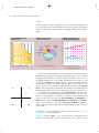
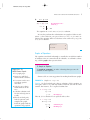
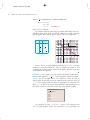
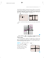
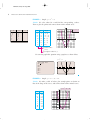
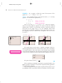
BG#5978, Composite Page 001
Introduction to Graphs
and the Graphing Calculator
●
●
●
Plot points by hand and using a grapher.
Graph equations by hand and using a grapher.
Find the point(s) of intersection of two graphs.
Graphing calculators and computers equipped with graphing software
are useful tools in applying and understanding mathematical concepts.
All such graphing utilities will be referred to as graphers in this
text, although the emphasis will be on graphing calculators.
When we think of the ways in which a grapher can be used, graphing
equations might come to mind first. Although the grapher will be used
extensively in this text to graph equations, many of its other uses will
also be explored. These include performing calculations, evaluating expressions, solving equations, analyzing the graphs of equations, creating
tables of data, finding mathematical models of real data, analyzing those
models, and using them to make estimates and predictions.
Keystrokes and features vary among different brands and models of
graphers. We will use features that are commonly found on many graphing calculators. Specif ic keystrokes and instructions for using these
features can be found in the Graphing Calculator Manual that accompanies this text. You can also consult either your instructor or the
user’s manual for your particular grapher.
The goal of this text is to use the grapher as a tool to enhance the
learning and understanding of mathematics and to relieve the tedium of
some procedures. Keep in mind that a grapher cannot be used effectively
without a f irm mathematical foundation upon which to build. For example, expressions cannot be entered correctly nor can results be interpreted well if the relevant concepts are not understood and applied
correctly.
The Use of the Grapher
A grapher is a tool that can be used in the process of learning and
understanding mathematics. It should be used to enhance the
understanding of concepts, not to replace the learning of skills.
1
BG#5978, Composite Page 002
2
INTRODUCTION
TO
GRAPHS
AND THE
GRAPHING CALCUL ATOR
Graphs
Graphs provide a means of displaying, interpreting, and analyzing data
in a visual format. It is not uncommon to open a newspaper or magazine
and encounter graphs. Shown below are examples of bar, circle, and line
graphs.
WORK PERMITS ISSUED
to Indiana Teens
SOURCES OF WATER
PERCENT UNINSURED vs.
PERCENT UNEMPLOYED
How we consume water
18%
64,772
1991
61,093
1992
Dairy
products
11%
77,982
1993
95,154
1994
115,708
1995
Drinking
water
38%
118,873
1998
0
40,000
80,000
Source: Indiana Department of Labor
y
II
Tea and coffee
30%
y
x
x
IV
% Uninsured
4%
% Unemployed
2%
0
Source: U.S. Department of Agriculture
(x, y)
12%
8%
120,000
I
14%
6%
111,934
1997
16%
10%
Vegetables
11%
109,308
1996
III
Soft drinks
10%
’88
’90
’92
’94
’96
Sources: U.S. Bureau of the Census;
U.S. Bureau of Labor Statistics
Many real-world situations can be modeled, or described mathematically, using equations in which two variables appear. We use a plane
to graph a pair of numbers. To locate points on a plane, we use two perpendicular number lines, called axes, which intersect at (0, 0). We call
this point the origin. The horizontal axis is called the x -axis, and the
vertical axis is called the y -axis. (Other variables, such as a and b, can
also be used.) The axes divide the plane into four regions, called quadrants, denoted by Roman numerals and numbered counterclockwise
from the upper right. Arrows show the positive direction of each axis.
Each point (x, y) in the plane is called an ordered pair. The first number, x, indicates the point’s horizontal location with respect to the y-axis,
and the second number, y, indicates the point’s vertical location with
respect to the x-axis. We call x the f irst coordinate, x -coordinate, or
abscissa. We call y the second coordinate, y -coordinate, or ordinate.
Such a representation is called the Cartesian coordinate system in
honor of the great French mathematician and philosopher René Descartes
(1596–1650).
EXAMPLE 1 Graph and label the points (3, 5), (4, 3), (3, 4), (4, 2),
(3, 4), (0, 4), (3, 0), and (0, 0).
Solution To graph or plot (3, 5), we note that the x-coordinate tells us
to move from the origin 3 units to the left of the y-axis. Then we move
BG#5978, Composite Page 003
INTRODUCTION
(3, 0)
5
(0, 4)
4
3
2
1
54321
1
2
(4, 2)
3
4
5
(3, 4)
(4, 3)
(0, 0)
1 2 3 4 5
(3, 4)
GRAPHS
AND THE
GRAPHING CALCUL ATOR
3
5 units up from the x-axis. To graph the other points, we proceed in a
similar manner. (See the graph at left.) Note that the origin, (0, 0), is located at the intersection of the axes and that the point (4, 3) is different
from the point (3, 4).
y
(3, 5)
TO
x
A graph of a set of points like the one in Example 1 is called a scatterplot. A grapher can also be used to make a scatterplot. This involves,
among other things, determining the portion of the xy-plane that will
appear on the grapher’s screen. That portion of the plane is called the
viewing window.
The notation used in this text to denote a window setting consists of
four numbers [L, R, B, T], which represent the Left and Right endpoints
of the x-axis and the Bottom and Top endpoints of the y-axis, respectively. The window with the settings [10, 10, 10, 10] is the standard
viewing window, shown in the following figure. On some graphers, the
standard window can be selected quickly using the ZSTANDARD feature
from the ZOOM menu.
10
WINDOW
Xmin 10
Xmax 10
Xscl 1
Ymin 10
Ymax 10
Yscl 1
Xres 1
10
10
10
ZOOM MEMORY
1: ZBox
2: Zoom In
3: Zoom Out
4: ZDecimal
5: ZSquare
6: ZStandard
7 ZTrig
S T U D Y
Xmin and Xmax are used to set the left and right endpoints of the
x-axis, respectively; Ymin and Ymax are used to set the bottom and top
endpoints of the y-axis. The settings Xscl and Yscl give the scales for the
axes. For example, Xscl 苷 1 and Yscl 苷 1 means that there is 1 unit between tick marks on each of the axes. Generally in this text, Xscl and
Yscl are both assumed to be 1 unless different values are given. Some exceptions will occur when the scaling factor is different from 1 but readily
apparent.
T I P
The Graphing Calculator
Manual that accompanies this
text gives keystrokes for
selected examples. See this
manual for the keystrokes to
use when entering points in
lists, setting up the STAT PLOT,
and graphing the points.
EXAMPLE 2 Use a grapher to graph the points (3, 5), (4, 3), (3, 4),
(4, 2), (3, 4), (0, 4), (3, 0), and (0, 0).
Solution We note that the x-coordinates of the given points range from
4 to 4 and the y-coordinates range from 4 to 5. Thus one good choice
for the viewing window is the standard window, because x- and y-values
both range from 10 to 10 in this window.
The coordinates of the points are entered into the grapher in lists
() key
using the EDIT operation from the STAT menu. Note that the ./
key must be used when we are entering negative num/
rather than the .
bers. We enter the first coordinates in one list, and then the corresponding second coordinates in the same order in a second list. Then we turn
BG#5978, Composite Page 004
4
INTRODUCTION
TO
GRAPHS
AND THE
GRAPHING CALCUL ATOR
on and set up a STAT PLOT to draw a scatterplot using the data from these
two lists.
10
L1
3
4
3
4
3
0
3
L2
5
3
4
2
4
4
0
L3
Plot1 Plot2 Plot3
On Off
Type:
______
Xlist: L1
Ylist: L2
Mark:
10
ⴙ
10
ⴢ
L2(1) 5
10
Some graphers have ZOOMSTAT a feature that automatically selects a
viewing window that displays all the data points in the lists for a given
STAT PLOT. This feature is activated after the data have been entered.
6.53
ZOOM MEMORY
3 Zoom Out
4: ZDecimal
5: ZSquare
6: ZStandard
7: ZTrig
8: ZInteger
9 ZoomStat
4.8
4.8
5.53
To turn off the plot, we return to the plot screen and select Off.
Solutions of Equations
Equations in two variables, like 2x 3y 苷 18, have solutions (x, y)
that are ordered pairs such that when the first coordinate is substituted
for x and the second coordinate is substituted for y, the result is a true
equation.
EXAMPLE 3 Determine whether each ordered pair is a solution of
2x 3y 苷 18.
a) (5, 7)
b) (3, 4)
Solution We substitute the ordered pair into the equation and determine
whether the resulting equation is true.
a)
2x 3y 苷 18
2(5) 3(7) ? 18
10 21
11
18
We substitute ⴚ5 for x and
7 for y (alphabetical order).
FALSE
The equation 11 苷 18 is false, so (5, 7) is not a solution.
BG#5978, Composite Page 005
INTRODUCTION
b)
TO
GRAPHS
AND THE
GRAPHING CALCUL ATOR
5
2x 3y 苷 18
2(3) 3(4) ? 18
6 12
18
18
We substitute 3 for x
and 4 for y.
TRUE
The equation 18 苷 18 is true, so (3, 4) is a solution.
We can also perform these substitutions on a grapher. When we substitute 5 for x and 7 for y, we get 11. Since 11 ⬆ 18, (5, 7) is not a solution of the equation. When we substitute 3 for x and 4 for y, we get 18,
so (3, 4) is a solution.
2(5)3ⴱ7
11
2ⴱ33ⴱ4
18
Graphs of Equations
The equation considered in Example 3 actually has an infinite number
of solutions. Since we cannot list all the solutions, we will make a drawing, called a graph, that represents them.
To Graph an Equation
Suggestions for
Hand-Drawn Graphs
1. Use graph paper.
2. Draw axes and label
them with the variables.
3. Use arrows on the axes
to indicate positive
directions.
4. Scale the axes; that is,
mark numbers on the
axes.
5. Calculate solutions and
list the ordered pairs in
a table.
6. Plot the ordered pairs,
look for patterns, and
complete the graph.
Label the graph with the
equation being graphed.
To graph an equation is to make a drawing that represents the
solutions of that equation.
Shown at left are some suggestions for making hand-drawn graphs.
EXAMPLE 4
Graph: 2x 3y 苷 18.
Solution To find ordered pairs that are solutions of this equation, we
can replace either x or y with any number and then solve for the other
variable. For instance, if x is replaced with 0, then
2 · 0 3y 苷 18
3y 苷 18
y 苷 6.
Dividing by 3
Thus (0, 6) is a solution. If x is replaced with 5, then
2 · 5 3y
10 3y
3y
y
苷
苷
苷
苷
18
18
8
8
3.
Subtracting 10
Dividing by 3
BG#5978, Composite Page 006
6
INTRODUCTION
TO
GRAPHS
AND THE
GRAPHING CALCUL ATOR
( 83) is a solution. If y is replaced with 0, then
Thus 5,
2x 3 · 0 苷 18
2x 苷 18
x 苷 9.
Dividing by 2
Thus (9, 0) is a solution.
We continue choosing values for one variable and finding the corresponding values of the other. We list the solutions in a table, and then
plot the points. Note that the points appear to lie on a straight line.
y
x
y
(x, y)
0
6
(0, 6)
5
8
3
(5, )
9
0
(9, 0)
1
20
3
(1, 203)
8
3
(1, c)
10
9
8
7
5
4
3
2
1
4321
1
2
3
4
2x 3y 18
(0, 6)
(5, h)
(9, 0)
1 2 3 4 5 6 7 8 9
x
In fact, were we to graph additional solutions of 2x 3y 苷 18, they
would be on the same straight line. Thus, to complete the graph, we use
a straightedge to draw a line as shown in the figure. That line represents
all solutions of the equation.
EXAMPLE 5 Use a grapher to create a table of ordered pairs that are solutions of the equation y 苷 12 x 1. Then graph the equation by hand.
Solution We use the TABLE feature on a grapher to create the table of
ordered pairs. We must first enter the equation on the equation-editor, or
“y 苷”, screen. Many graphers require an equation to be entered in the
form “y 苷” as this one is written. If an equation is not initially given in
this form, it must be solved for y before it is entered in the grapher.
Plot1 Plot2 Plot3
\ Y1 (1/2)X1
\ Y2 \ Y3 \ Y4 \ Y5 \ Y6 \ Y7 On a grapher, we enter y 苷 (1兾2)x 1. Since 1兾2x is interpreted as
(1兾2)x by some graphers and as 1兾(2x) by others, we use parentheses to
BG#5978, Composite Page 007
INTRODUCTION
TO
GRAPHS
AND THE
GRAPHING CALCUL ATOR
7
ensure that the equation is interpreted correctly. Then we set up a table
in AUTO mode by designating a value for TBLSTART and a value for TBL.
The grapher will produce a table starting with the value of TBLSTART and
continuing by adding TBL to supply succeeding x-values. For the equation y 苷 12 x 1, we let TBLSTART 苷 3 and TBL 苷 1.
TABLE SETUP
TblStart 3
Tbl 1
Indpnt: Auto Ask
Depend: Auto Ask
X
3
2
1
0
1
2
3
X 3
Y1
.5
0
.5
1
1.5
2
2.5
Next, we plot some of the points given in the table and draw the
graph.
y
y qx 1
5
4
3
2
(2, 0)
54
21
1
2
3
4
5
(2, 2)
(0, 1)
1 2 3 4 5
x
In the equation y 苷 12 x 1, the value of y depends on the value
chosen for x, so x is said to be the independent variable and y the dependent variable.
We can also graph an equation on a grapher. Be sure that the stat
plots are turned off, as described on p. 4, before graphing equations like
those below. Failure to do this could affect the viewing window and prevent the desired graph from being seen.
EXAMPLE 6 Graph using a grapher: y 苷 12 x 1.
Solution We enter y 苷 12 x 1
on the equation-editor screen in
the form y 苷 (1兾2)x 1, select
a viewing window, and draw
the graph. The graph is shown
in the standard window.
y qx 1
10
10
10
10
BG#5978, Composite Page 008
8
INTRODUCTION
TO
GRAPHS
AND THE
GRAPHING CALCUL ATOR
EXAMPLE 7 Graph: y 苷 x 2 5.
Solution We select values for x and find the corresponding y-values.
Then we plot the points and connect them with a smooth curve.
y
X
3
2
1
0
1
2
3
X 3
Y1
4
1
4
5
4
1
4
x
y
(x, y)
3
2
1
0
1
2
3
4
1
4
5
4
1
4
(3, 4)
(2, 1)
(1, 4)
(0, 5)
(1, 4)
(2, 1)
(3, 4)
y x2 5
5
4
3
2
1
(3, 4)
543
(2, 1)
(3, 4)
1
1
2
3
(1, 4)
1
3 4 5
(2, 1)
x
(1, 4)
(0, 5)
嘷
1 Select values
for x.
嘷
2 Compute values for y.
We can also graph this equation using a grapher, as shown below.
y x2 5
6
Plot1 Plot2 Plot3
\ Y1 X25
\ Y2 \ Y3 \ Y4 \ Y5 \ Y6 \ Y7 6
6
6
EXAMPLE 8 Graph: y 苷 x 2 9x 12.
Solution We make a table of values, plot enough points to obtain an
idea of the shape of the curve, and connect them with a smooth curve.
y
x
y
3
1
0
2
4
5
10
12
24
2
12
26
32
32
2
24
y x2 9x 12
20
15
10
5
864
2 4 6 8
15
20
25
30
12
x
BG#5978, Composite Page 009
INTRODUCTION
TO
GRAPHS
AND THE
GRAPHING CALCUL ATOR
9
We can also graph the equation using a grapher. We enter y 苷 x 2 9x 12 on the equation-editor screen and graph the equation in the
standard window.
y x2 9x 12
10
10
10
10
Note that this window does not give a good picture of the graph. Because the graph is cut off to the right of x 苷 10 and below y 苷 10, it
appears as though Xmax should be larger than 10 and Ymin should be
less than 10. Since the graph rises steeply in the second quadrant, we
could also let Xmin be 5 rather than 10. We try [5, 15, 15, 10],
with Yscl 苷 2.
y x2 9x 12
10
5
15
15
Yscl 2
The graph is still cut off below Ymin, or 15. We try other settings
for Ymin until we find one that shows the lower portion of the graph.
One good window is [5, 15, 35, 10], with Yscl 苷 5.
y x2 9x 12
10
5
15
35
Yscl 5
Finding Points of Intersection
There are many situations in which we want to determine the point(s) of
intersection of two graphs.
BG#5978, Composite Page 010
10
INTRODUCTION
TO
GRAPHS
AND THE
GRAPHING CALCUL ATOR
EXAMPLE 9 Use a grapher to find the point of intersection of the
graphs of x y 苷 5 and y 苷 4x 10.
Solution Since equations must be entered in the form “y 苷” on many
graphers, we solve the first equation for y:
x y 苷 5
x苷y5
x 5 苷 y.
Adding y on both sides
Adding 5 on both sides
Now we can enter y1 苷 x 5 and y2 苷 4x 10 on the equationeditor screen and graph the equations. We begin by using the standard
window and see that it is a good choice because it shows the point of
intersection of the graphs. Next, we use the INTERSECT feature from
the CALC menu to find the coordinates of the point of intersection. (See
the Graphing Calculator Manual that accompanies this text for the
keystrokes.)
y1 x 5, y2 4x 10
y2 10
10
Plot1 Plot2 Plot3
\ Y1 X5
\ Y2 4X10
\ Y3 \ Y4 \ Y5 \ Y6 \ Y7 10
10
RATIONAL NUMBERS
10
10
y1
y2
REVIEW SECTION R.1.
y1
Intersection
X 1.666667
Y 3.3333333
10
10
The graphs intersect at the point (1.666667, 3.3333333), which is a
decimal approximation for the point of intersection. If the coordinates
are rational numbers, their exact values can be found using the 䉴FRAC
feature from the MATH menu. (The keystrokes for doing these conversions
are given in the Graphing Calculator Manual that accompanies this text.)
X Frac
5/3
Y Frac
10/3
(
The point of intersection is 53 ,
10
3
).
If the coordinates in Example 9 had not been rational numbers, the
operation would have returned the original decimal approximation rather than a fraction.
If a pair of equations has more than one point of intersection, we use
the INTERSECT feature repeatedly to find the coordinates of all the points.
䉴FRAC