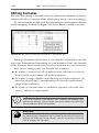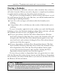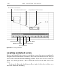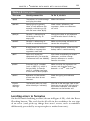
1
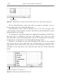
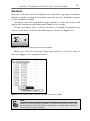
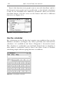
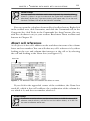
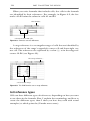
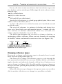
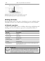
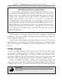
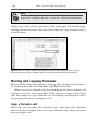
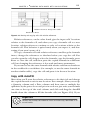
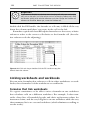
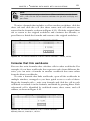
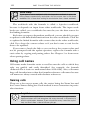
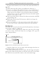
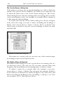
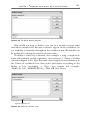
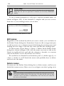
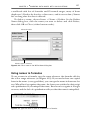
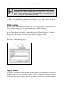
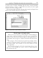
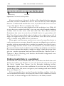
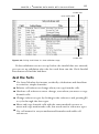
AL TE RI Working Data Magic with Calculations O PY RI GH TE D MA nce data is entered in a workbook, you’re ready to perform calculations on it (after all, calculations are why Excel exists). To perform calculations in a worksheet, you write formulas; to perform complex calculations, you use functions in your formulas (functions are built-in mathematical equations that save you time and effort, and are covered in Chapter 5). This chapter is full of basic calculation information: getting fast answers without formulas, writing your own formulas, using cell references and cell names for better calculation control, and fixing errors. It could just as well have been titled “Calculations 101.” Simple calculations, quick answers CO To get really quick answers without writing a formula yourself, you have two options: AutoCalculate, which calculates cells in the worksheet temporarily but doesn’t write formulas; and AutoSum, which writes very simple formulas in the worksheet very quickly. AutoCalculate AutoCalculate is a handy tool that I use often to calculate cells on the fly while I work. The AutoCalculate box is near the right end of the Excel Status bar, shown in Figure 4.1. 109 Chapter 4 GET THE SCOOP ON... Simple calculations and quick answers ■ Cell references ■ Writing formulas ■ Moving and copying formulas ■ Linking workbooks with formulas ■ Cell names ■ Editing formulas ■ Auditing formulas ■ Locating worksheet errors 110 PART II ■ GETTING THE DATA IN AutoCalculate Figure 4.1. AutoCalculate is always at work. All you need to do is select two or more cells. To use AutoCalculate, select the cells you want to calculate (two or more) and look at the AutoCalculate box. AutoCalculate sums cells by default, but it can also average cells, count entries, count numeric entries, and tell you the maximum or minimum number in a range. To change the calculation function, right-click anywhere in the Status bar and select a different function (see Figure 4.2). You can turn AutoCalculate off by selecting None, but it’s so unobtrusive that many people never even notice it, so why bother turning it off? If there’s no display in the AutoCalculate box (and it’s not turned off), that’s because you only have one cell selected, or you don’t have appropriate data selected for the current AutoCalculate function. For example, if you only have text cells selected, only the Count function works. Right-click anywhere in the Status bar Figure 4.2. Changing the AutoCalculate function CHAPTER 4 ■ WORKING DATA MAGIC WITH CALCULATIONS 111 AutoSum To enter a formula in the worksheet that calculates a group of numbers without actually writing the formula yourself, use the AutoSum button on the Standard toolbar. AutoSum can write sum and average numbers, count all entries, and display the maximum and minimum numbers in a range. To use AutoSum, click a cell directly below a column of numbers you want to sum, then click the AutoSum button (shown in Figure 4.3). Figure 4.3. The AutoSum button on the Standard toolbar Make sure that the moving border surrounds the cells you want to sum (see Figure 4.4), and press Enter. Figure 4.4. The moving border surrounds the cells that will be summed. Hack AutoSum can write a formula anywhere and calculate any cells you select. Click the cell where you want the formula, click AutoSum, and then drag or Ctrl+click all the cells you want to calculate. 112 PART II ■ GETTING THE DATA IN Sum is the function most people want to use with AutoSum (and it’s the function most people use in a workbook), so the default calculation is sum. To use AutoSum with a different calculation, when you click the AutoSum button, click the arrow on the button and select a different function (see Figure 4.5). Figure 4.5. Change the AutoSum function. Use the calculator For calculations on the fly that don’t require any worksheet data, use the Windows calculator (see Figure 4.6). You’ve probably seen and used the calculator — it’s available in the Start Programs Accessories menu. The calculator is a plain-Jane sort and fairly limited, but its simplicity is what makes it convenient, and it’s what I use when I want to calculate something simple without typing data into a worksheet. Figure 4.6. The Windows calculator CHAPTER 4 Inside Scoop ■ WORKING DATA MAGIC WITH CALCULATIONS 113 Inside Scoop You can make the calculator much more high-tech by choosing View Scientific (I leave it to you to understand the higher-level mathematics available there). By the way, if you want to do a quick square root, it’s on the small Standard calculator, but not on the Scientific calculator. You can open the calculator from an Excel toolbar button. Right-click in the toolbar area, click Customize, and click the Commands tab; in the Categories list, click Tools; in the Commands list, drag Custom (the one with the calculator icon) to your toolbar. Read more about toolbars and buttons in Chapter 21. About cell references A cell reference is the cell’s address on the worksheet in terms of its column letter and row number. You can tell what any cell’s reference is by either looking at the row and column that intersect at the cell or by selecting the cell and looking at the Name box (see Figure 4.7). Name box Figure 4.7. The Name box shows the selected cell address or name. If you click in the upper-left corner of the worksheet, the Name box reads A1, which is that cell’s address: the combination of the column letter, which is A, and the row number, which is 1. Inside Scoop Inside Scoop To reference an entire column, use the column letter, as in B:B for column B. To reference several columns, use the first and last column letters, as in B:D. Do the same to reference entire rows. 114 PART II ■ GETTING THE DATA IN When you write formulas that include cells, the cells in the formula are identified by their references. For example, in Figure 4.8, the formula =A1+B1 sums the values in cells A1 and B1. This formula... ...references these two cells. Figure 4.8. Formulas use cell references. A range reference is a rectangular range of cells that are identified by the references of the range’s upper-left corner cell and lower-right corner cell. The references are separated by a colon (:), as in the range reference A1:B6 (see Figure 4.9). This range reference... ...refers to this range. Figure 4.9. This SUM formula uses a range reference. Cell reference types Cells can have different types of references, depending on how you want to use them in the formula. First, I explain the terminology and how to create the different types; then I show you how they work with actual examples (at which point they’ll make more sense). CHAPTER 4 ■ WORKING DATA MAGIC WITH CALCULATIONS 115 For any cell, there is only one reference but four reference types: relative, absolute, and two mixed types. Dollar signs ($) in the reference determine the type: ■ A1 is called relative. ■ $A$1 is called absolute. ■ $A1 and A$1 are called mixed. An absolute cell reference is a fixed geographical point, like a street address, such as 123 Cherry Street. A relative cell reference is a relative location, as in “one block west and two blocks south.” The mixed cell reference is a mixture of absolute and relative locations, as in “three blocks east on Hampden Avenue.” A mixed cell reference can have an absolute column and relative row, as in $A1, or a relative column and absolute row, as in A$1. The dollar signs designate the row and/or column as absolute, or unchanging, within a reference. When you write formulas, the meetings of absolute, relative, and mixed become more clear (see Figure 4.10). Relative Absolute Mixed Figure 4.10. The four reference types Changing reference types If you need to change a cell reference type in a formula, there’s a much faster way than typing dollar signs ($). The fastest way to change cell reference types is to cycle through the four types until you find the one you want: Double-click the cell containing the formula, and within the formula, click in the cell reference you want to change (see Figure 4.11). Press F4 until the reference changes to the type you want (pressing F4 repeatedly cycles through all the possible reference types). When the reference type changes to the type you want, you can either click in another cell reference to change it or press Enter to finish. 116 PART II ■ GETTING THE DATA IN Click in reference and press F4 Figure 4.11. Open the cell, click in the reference (in the cell or in the Formula bar), press F4 to cycle, and press Enter. Writing formulas You’ll probably need to do more calculations in your workbooks than AutoSum can do for you, which means learning how to write formulas. Arithmetic operators A simple formula might consist of adding, subtracting, multiplying, and dividing cells. Excel’s arithmetic operators are detailed in Table 4.1. Table 4.1. Arithmetic operators Operator Description + (plus sign) Addition – (minus sign) Subtraction * (asterisk) Multiplication / (forward slash) Division ^ (caret) Exponentiation () (parentheses) To group operations, such as =(2+3)*4, which gives a different result than =2+3*4 Bright Idea Here’s a formula that uses arithmetic operators and a simple function to calculate the circumference of a circle, rr2: =PI()*ref^2. Specify a cell in the ref argument and type the radius of the circle in that cell; then you can use this formula repeatedly by changing the radius entered in the ref cell. CHAPTER 4 ■ WORKING DATA MAGIC WITH CALCULATIONS 117 Cell references versus static entries Occasionally you’ll want to write formulas that include a static (constant, not calculated) entry such as a sales tax rate or a product name, but it’s more efficient to write formulas that only use cell references. For example, if you want to write a formula that totals prices and calculates sales tax, you can write a formula like =SUM(F6:F17)* .07, but when the tax rate changes, you must open all the formulas that use the sales tax rate and change it in every formula. However, if you put the tax rate in a cell and reference that cell in your formulas, you need only to change the tax rate in the cell, and all the formulas that reference the tax rate cell are instantly updated. All formulas can calculate cells in the same worksheet, on different worksheets, and even in different workbooks (which links the workbooks and worksheets together). Some simple formulas have to be written by you; there’s no easy automatic feature to write them for you. But writing your own simple formulas is, well, simple. For example, a subtraction formula has to be written by you. Simple formulas To write a simple formula that calculates two cells (for example, subtracting one cell from another), click the cell where you want to display the results, type an equal sign (=), click one of the cells you want to use, type your arithmetic operator, click the second cell you want to use, and press Enter. The simple formula is entered, as shown in Figure 4.12. When you build a formula by clicking cells and dragging ranges, the cells have relative references. What the formula in Figure 4.12 really does is subtract the cell two cells above from the cell three cells above the current Watch Out! Always click a cell to enter it in a formula; typing cell references is laborious and error prone. 118 PART II ■ GETTING THE DATA IN Hack You can quickly show all the formulas in a worksheet if you press Ctrl+` (the grave accent on the same key as the tilde (~). Press Ctrl+` again to hide the formulas. cell because of the relative references. The advantages and disadvantages of using relative references become clear when you copy formula cells to a new location. Figure 4.12. This formula subtracts one date (in cell D2) from another date (in cell D3) to how the number of days between; there’s no quick automated tool for subtraction. Moving and copying formulas You use all the same techniques for moving and copying formula cells as for nonformula cells, but sometimes with different results. When you move a formula cell, the formula moves intact and the cell references stay the same regardless of the reference types of the input cells. But when you copy a formula cell, bad things can happen if you’re not prepared for them (see Figure 4.13). Copy a formula cell When you copy formulas, the reference type comes into play. Absolute references do not adjust when you copy a formula; they always calculate the same input cells. CHAPTER 4 ■ WORKING DATA MAGIC WITH CALCULATIONS 119 Relative references changed the results Results still correct Figure 4.13. Moving and copying cells with relative references Relative references, on the other hand, give the input cells’ locations relative to the formula cell, and when you copy a formula cell to a new location, relative references continue to refer to locations relative to the formula cell. This behavior is quite handy when you expect it, and frustrating if you aren’t aware of it. To copy a formula cell with relative references and keep the formula intact, change the references to absolute before you copy the cell. You can also open the cell, drag to select the formula, copy the formula, press Enter to close the cell, and then paste the copied formula in a different cell, but changing the references is less work and more permanent. If you want to use the same formula with relative references elsewhere in the workbook or worksheet (for example, to use the same formula in another similar table), copy the cell and paste it in the new location. Copy with AutoFill Most often you’ll want the relative references to do their job and change the copied formula to suit its new location. For example, when you set up a Quantity column and a Price column and then want to multiply the quantities by the prices for a total price in each row, just write your formula one time at the top of the total column, and click and drag the AutoFill handle down the column to fill the formula cells (see Figure 4.14). If you Bright Idea The best way to keep cell references intact and also easily identifiable is to use cell names. 120 PART II ■ GETTING THE DATA IN Bright Idea If you want a formula to calculate one changing cell with one unchanging cell, such as the cells in a Price column and an unchanging TaxRate cell, write the formula quickly with relative references and then change the TaxRate cell reference to absolute. Better yet, name the TaxRate cell. double-click the Fill handle, the formula or cell entry is filled all the way down the column until there’s no entry in the cell to the left. Formulas copied with AutoFill adjust themselves so that every relative reference refers to the correct cell relative to the formula cell (the relative references do the adjusting). Fill handle Figure 4.14. Click and drag or double-click the Fill handle to copy the formula down the column. Linking worksheets and workbooks You can write formulas that reference cells in other worksheets or workbooks; those formulas link the worksheets or workbooks. Formulas that link worksheets It’s a great convenience to be able to write a formula on one worksheet that calculates cells on a different worksheet. For example, I often transcribe client lists of household goods and their replacement values for insurance claims, and the very long list is on one worksheet while the very short summary list is on a second worksheet (which eliminates scrolling to see the totals). CHAPTER 4 ■ WORKING DATA MAGIC WITH CALCULATIONS 121 Hack If you only need to display a value from a different worksheet, start the formula with =, then click the cell on the other worksheet that you want to display and press Enter. To write a formula that includes a cell on another worksheet, click the sheet tab and click the cell (the sheet name and cell reference are entered in the formula, as shown in Figure 4.15). Click the original sheet tab to return to the original worksheet and continue the formula, or press Enter to finish the formula and return to the original worksheet. Figure 4.15. This formula references a cell on another worksheet — Sheet3, cell C5. Formulas that link workbooks You can also write formulas that calculate cells in other workbooks. For example, if you have workbooks that represent sales from different districts, you can write a formula in another workbook that sums values from the district workbooks. To write a formula that links workbooks, open all the workbooks in multiple windows, arranged so you have quick access to each of them. Begin the formula with =, write your formula and click the cell in each workbook to include it in the formula, and finish by pressing Enter. Each referenced cell is identified by workbook name, sheet name, and cell address, as shown in Figure 4.16. Figure 4.16. This formula references a cell in another workbook — Quarterly Sales.xls, sheet Qtr 1, cell C71. 122 Inside Scoop PART II ■ GETTING THE DATA IN Inside Scoop If you open a source workbook while the dependent workbook is open, the linking formula automatically recalculates with the current data in the source workbook. This is faster than waiting for recalculation from a closed workbook. The workbook with the formula is called a dependent workbook, because it depends on input from other workbooks. The input workbooks are called source workbooks because they are the data source for the linking formulas. Each time you open a dependent workbook, you are asked if you want to update it with linked information from the other workbooks. Click Yes to update the linked formulas with current data in the other workbooks; click No to keep the current values or if you don’t want to wait for the data to be updated. If you want to break the link so you can keep the current value and not be prompted with the update question, replace the formula with a static value by copying and pasting values. See Chapter 3 to learn more about pasting values. Using cell names Cell names make formulas easier to read because the cells to which they refer are quickly and easily identified (for example, the formula =Subtotal+Tax is easier to understand than =G19+G20). Also, cell names keep cell formulas intact when the formulas reference cell names because cell names are always created with absolute references. Naming cells There are a few ways to name cells, the easiest being the Name box and the Create Names dialog box. Each method is most convenient in particular situations. Bright Idea Always use some capital letters in a name, because when you type a name in lowercase letters and Excel recognizes the name, the name is switched to its official capitalization. However, if you misspell the name, it won’t be capitalized, and that’s often a clue to the error you get. CHAPTER 4 ■ WORKING DATA MAGIC WITH CALCULATIONS 123 No matter what method you use to name cells, names must follow certain rules: ■ Names must start with a letter or an underscore character (_). ■ No spaces are allowed. For multiword names, use an underscore or, better yet, use initial capital letters to separate words, as in LastName. Names are not case sensitive, so if you type the name in a formula, you don’t have to type the capital letters; however, the initial capitals make the name easier to read. ■ Don’t use periods. They’re allowed, but they may interfere with VBA programming code. ■ Keep names shorter than 255 characters (which is too long to be practical, anyway). ■ Do not use hyphens or other punctuations marks (if Excel doesn’t let you create a name, a punctuation mark may be the problem). The Name box The Name box, located on the left end of the Formula bar, is the fastest way to name a range or a single cell. To name a cell or range with the Name box, select the cell or range you want to name, click in the Name box (see Figure 4.17), type the name, and press Enter. Name box Selected cell being named Figure 4.17. Click in the Name box, type a name, and press Enter. Using the Name box, you can name cells and ranges that have no identifying headings on the worksheet. No matter what method you use to name cells and ranges, the names appear in the Name box list when you click the arrow next to the Name box. Click the arrow and click a name to select the named range. 124 PART II ■ GETTING THE DATA IN The Create Names dialog box If the names you want to use are already headings in a table or labels for specific cells (such as Total or TaxRate), the fastest way to name the cells to which the labels refer is the Create Names dialog box. The Create Names dialog box not only uses existing names (no typing), but it can also create several names at once (for example, it can name all the columns in a table using the table headings). To name cells with the Create Names dialog box (shown in Figure 4.18), select the range you want to name (including the headings or labels), then choose Insert Name Create. Select or deselect the check boxes as needed so that the correct headings or labels are used, and click OK. Figure 4.18. The Create Names dialog box The names are created, and you can select any of the named ranges by clicking its name in the Name box list. The Define Name dialog box The Define Name dialog box is not a good choice for naming cells (it’s too laborious), but it’s the only way you can name constant values and formulas, edit the definition of an existing name, or delete a name. To define a name for a constant value (for example, a tax rate), choose Insert Name Define. Type the name (for example, TaxRate) in the Names in workbook box (shown in Figure 4.19); then select and delete everything in the Refers to box (including =), and type =your value (for example, =0.75). Click OK (not Close). CHAPTER 4 ■ WORKING DATA MAGIC WITH CALCULATIONS 125 Figure 4.19. The Define Name dialog box Why would you want to define a tax rate in a named constant value instead of a named cell? Because it doesn’t appear in the worksheet, yet it is available to formulas throughout the workbook and all formulas can be updated by editing the named constant value. To define a name for a formula (for example, a long, complex formula with multiple nested segments), choose Insert Name Define (shown in Figure 4.20). Type the name (for example, InvoiceNumber) in the Names in workbook box; then select and delete everything in the Refers to box (including =). Type =your formula (for example, =LEFT(A3,3)&”-”&RIGHT(H5,4) ). Click OK (not Close). Type the formula here Figure 4.20. Defining a formula name 126 Inside Scoop PART II ■ GETTING THE DATA IN Inside Scoop You won’t see formula or constant names in the Name box or the Apply Names dialog box, but you can type them in formulas (so use easily remembered names). To use a named formula in a cell, type = and the formula name (as shown in Figure 4.21). If the formula is complex and you use it more than once a year, naming it saves a lot of time. Figure 4.21. Using a named formula in a cell Edit names Regardless of the method by which you create a name, you can find it in the Define Name dialog box. Sometimes I want to edit a range name just to add an extra row or column; instead of deleting the existing name and naming the new range, I take the fast route and edit the existing name. To edit a name, choose Insert Name Define. In the Define Name dialog box, shown in Figure 4.22, click the name you want to edit in the Names in workbook box, and edit the reference, formula, or constant value in the Refers to box. Press Enter (not Close). Be careful not to disturb the exclamation point (!), dollar sign ($), or colon (:) marks or you’ll break the name and probably have to delete and re-create the name. Delete names You must use the Define Name dialog box to delete names, and lest you think this is unnecessary, I dare you to try to figure out what’s going on in Hack If you want to keep a name definition but change the name, you must add the new name and delete the old. The safest way is to select the old name and type a different name in the Names in workbook box, then click Add, then select the old name and click Delete. CHAPTER 4 ■ WORKING DATA MAGIC WITH CALCULATIONS 127 a workbook with lots of formulas and 85 named ranges, many of them duplicates! (I had to do that for a client once, and it was not fun.) Names live on long after the data is deleted. To delete a name, choose Insert Name Define. In the Define Name dialog box, click the name you want to delete and click Delete, then click OK or Close (either button works). Select the name Edit the name’s reference Figure 4.22. Edit a name in the Define Name dialog box. Using names in formulas To use a name in a formula, type the name wherever the formula calls for the cell or range reference (see Figure 4.23). If you used at least one capital letter in the name (a very good idea), you can type the name in lowercase letters. When Excel recognizes the name, the letters are switched to their original capitalization. If you misspell the name, Excel won’t recognize it. You get an error, and the lack of capitalization tells you that the name is misspelled. Figure 4.23. Type the name in place of a reference in a formula. 128 Inside Scoop PART II ■ GETTING THE DATA IN Inside Scoop If you want to remember what all of your names refer to without slogging through the Define Name dialog box, you can paste a list of all the workbook names and their definitions onto a worksheet. Click a cell, choose Insert Name Paste, and click the Paste List button. You can type defined names in formulas as you write them, or in the Function Arguments dialog box (covered in Chapter 5). Paste names If you can’t remember the name, or it’s a long name, you can use the Paste Name dialog box to paste the name into the formula. To paste names into a formula, start the formula, and place the insertion point where you want to insert the name. Choose Insert Name Paste, click the name, and then click OK (see Figure 4.24). If you don’t mind memorizing another keystroke, it’s faster to click in the reference you want to replace with a name and then press F3 to open the Paste Names dialog box. Figure 4.24. Paste names instead of typing them. Apply names If you’ve already written formulas using normal cell references instead of named cells, you can quickly change all the named cell references in a worksheet into their names. Select the range of cells that contain formulas CHAPTER 4 ■ WORKING DATA MAGIC WITH CALCULATIONS 129 (as many cells as you like, including cells that don’t contain formulas), and choose Insert Name Apply. Click every name you want to apply and then click OK (see Figure 4.25). You can even name cells after you write the formulas and apply those names to the formulas that have cell references. Figure 4.25. Apply names to replace references in formulas. Named ranges and apply names When you create names in a table using the table headings as range names, and then AutoFill or otherwise copy a formula that references the cells in those named ranges and then apply names to the formulas, what you get is a column of formulas that all look the same. For example, a Total column has formulas that multiply a Price column by a Quantity column, and the Price and Quantity columns are named ranges. The formulas in the Total column all read =Price*Quantity. Each formula is using the cells in the named range that are in its own row, so the formulas are correct, even if it’s unnerving that they all look the same. 130 PART II ■ GETTING THE DATA IN Editing formulas You can easily change a formula in any way (function, arithmetic operators, referenced cells, or constant values, which pretty much covers everything). To edit a formula, double-click the cell and select and replace whatever needs changing, as shown in Figure 4.26. Press Enter to finish your edits. Figure 4.26. You can edit a formula in the cell or in the Formula bar. Editing a formula is often easier if you click the cell and do your editing in the Formula bar. Depending on your worksheet font, the formula in the Formula bar is nearly always easier to read and use your mouse in. Easy ways to change parts of a formula are as follows: ■ To replace a referenced cell, double-click the reference to select it, then click the replacement cell in the worksheet. ■ To replace a range, double-click and drag over both references (to select the whole range), and then drag to select the replacement range in the worksheet. ■ To replace a constant value or arithmetic operator, select the character(s) and type a replacement. Bright Idea If you want to replace a cell reference with a different cell reference, don’t type the new reference; instead, double-click the old reference and then click the new reference cell on the worksheet. Watch Out! Be careful not to click other cells unintentionally while a cell is open for editing, because those unintentional cells are added to your formula. If you inadvertently add other cells to your formula, press Esc to back out of the cell with no changes, and start again. CHAPTER 4 ■ WORKING DATA MAGIC WITH CALCULATIONS 131 Tracing a formula In some worksheets, formulas reference other formulas that reference still other formulas. When you need to dig into a complicated worksheet to understand its architecture, Excel has tools to help you. The process of tracing formulas is called auditing, and there’s a toolbar with buttons that do the work. But first, you should understand the terminology of auditing formulas: ■ A precedent cell is an input cell referenced in the formula you’re auditing. ■ A dependent cell is a cell that uses the results of the formula you’re auditing. To trace a formula, right-click in the toolbar area and click Formula Auditing to show the Formula Auditing toolbar. Then click the cell with the formula you want to trace (see Figure 4.27). Then: ■ To trace precedents, click the Trace Precedents button. The first level back is shown by blue lines that connect the formula cell to all its input cells. Click the Trace Precedents button again to trace the next level back, and continue clicking the Trace Precedents button until no new blue lines appear. ■ To trace dependents, click the Trace Dependents button. The first level forward is shown by blue lines that connect the formula cell to all its dependent cells. Click the Trace Dependents button again to trace the next level forward, and continue clicking the Trace Dependents button until no new blue lines appear. To erase the precedent or dependent lines one generation at a time, click the Remove Precedent Arrows button and the Remove Dependent Arrows button. To remove all the lines so you can trace another cell, click the Remove All Arrows button. Bright Idea To see the immediate precedent cells for a formula, double-click the formula cell. The cell references in the open cell are colored; the colors correspond to the colored outlines around the referenced cells and ranges. Press Enter or Esc to close the cell without changing the formula. 132 PART II ■ GETTING THE DATA IN Precedents back two levels Precedents back one level Trace Precendents Dependents forward one level Remove All Arrows Remove Precendents Remove Dependents Trace Dependents Figure 4.27. Tracing a formula Locating worksheet errors Errors and invalid data seem to sneak into even the most scrupulously designed and maintained worksheets. You can find them with the help of a few tools on the Formula Auditing toolbar. If you see an error, refer to Table 4.2, which provides a list of what the errors mean and how to fix them. To show the Formula Auditing toolbar, right-click in the toolbar area and click Formula Auditing. CHAPTER 4 ■ WORKING DATA MAGIC WITH CALCULATIONS 133 Table 4.2. Error values This error Usually means this To fix it, do this ##### The column isn’t wide enough to display the value. Widen the column. #VALUE! Wrong type of argument, value, or cell reference (for example, calculating a cell with the error value #N/A). Check values, references, and arguments; make sure references are valid. #DIV/0! Formula is attempting to divide by zero or by an empty cell. Change the value or cell reference so the formula doesn’t divide by zero. #NAME? Formula is referencing an invalid or nonexistent name. Make sure the name still exists or correct the misspelling. #N/A Usually means no value is available or inappropriate arguments were used. In a lookup formula, make sure the lookup table is sorted correctly. #REF! Excel can’t locate the Click Undo immediately to restore referenced cells (for example, references, and then change if referenced cells are deleted). formula references or convert formulas to values. #NUM! Incorrect use of a number (such as SQRT(-1), which is not possible), or formula result is a number too large or too small to be displayed. Make sure that the arguments are correct, and that the result is between –1*10307 and 1*10307. #NULL! Reference to intersection of two areas that do not intersect. Check for typing and reference errors. Circular reference message The formula refers to itself, either directly or indirectly. Click OK in the message; look at the Status bar to see which cell contains the circular reference, and remove references to the formula cell. Locating errors in formulas On the Formula Auditing toolbar (shown in Figure 4.28), click the Error Checking button. The tool checks all cells in the worksheet for any sign of an error (and picks up things that aren’t errors, such as numbers deliberately preceded by an apostrophe to make them text). 134 Error Checking PART II ■ GETTING THE DATA IN Trace Error Figure 4.28. The Formula Auditing toolbar If a perceived error is located, the Error Checking dialog box appears and tells you what it thinks the error is. You can use any of the helpful buttons to understand and fix the error; if you know the error is not an error, click Ignore Error to continue the check. If you have an error value displayed on the worksheet (see Table 4-2 to see what error values look like), you can open the Formula Auditing toolbar, click in the error cell, and click the Trace Error button. Sometimes the error is not in the cell itself, but is in a precedent cell. The Trace Error button finds what it thinks is the culprit input cell. It might or might not help you, but you still have to fix the error yourself after it’s found, using Table 4-2 as a reference. Then again, you may never need to trace errors, because Excel tries to catch your errors as you enter them. If you enter an alleged error, such as a number with an apostrophe first to make the number text, Excel pops a green triangle into the corner of the cell and when you click the cell you get an error button in the worksheet as well. You can click the error button for a shortcut menu that might or might not help. I think the green triangles are a useless intrusion and turn them off like this: Choose Tools Options Error Checking, and deselect the Enable background error checking check box. Finding invalid data in a worksheet If someone has entered invalid data into a worksheet in which data validation is in effect (see Chapter 3), you can locate the inaccuracies with the Circle Invalid Data button on the Formula Auditing toolbar. (Remember, when you set data validation, if you don’t use the Stop style on the Error Alert tab, users can ignore your warnings and enter invalid data; see Chapter 3.) To locate invalid data, on the Formula Auditing toolbar, click the Circle Invalid Data button. All entries that don’t meet validation criteria are circled, as shown in Figure 4.29. You have to fix them yourself. CHAPTER 4 ■ WORKING DATA MAGIC WITH CALCULATIONS 135 Invalid data Circle Invalid Data Invalid data Figure 4.29. Circling invalid data in a data-validation range If data validation was not set up before the invalid data was entered, you can set up validation after the fact and then run the Circle Invalid Data button to find the bad data. Just the facts ■ Use AutoCalculate for instant, on-the-fly calculations and AutoSum to write fast, simple formulas. ■ Relative cell references change when you copy formula cells. ■ Absolute cell references never change, even when you move or copy formula cells. ■ Change reference types by clicking in the reference and pressing F4 to cycle through the four types. ■ Move and copy formula cells with the same methods you use to move and copy nonformula cells, but watch out for reference types. ■ Use cell names for easy-to-understand formulas and stable cell references. 136 PART II ■ GETTING THE DATA IN ■ Edit formulas by double-clicking to edit in the cell, or clicking to edit in the Formula bar. ■ Locate errors and invalid data with the buttons on the Formula Auditing toolbar.