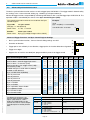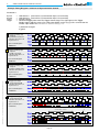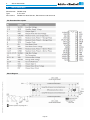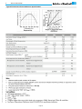
Download Sch"after+Kirchhoff SK1024U3PD Instruction manual

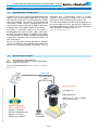
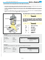
USB 3.0
SK1024U3PD
Monochrome Line Scan Camera
1024 pixels, 10 µm x 10 µm, 50 / 25 MHz pixel frequency
• Robust cable connections
• Hot-pluggable
• Perfect for movable setups
Instruction Manual
Schäfter + Kirchhoff © 2014 • Line Scan Camera SK1024U3PD Manual (05.2014) • shared_Titel_AT1.indd (05.2014)
05.2014
Sample Configuration
1 SK1024U3PD
mounted with
2 3 4 3
CCD line scan camera
Mounting bracket SK5105
1
Clamping claws SK5102
Video (CCTV)-objectiv
2
4
Read the manual carefully before the initial start-up. For the content table refer to page 2.
The producer reserves the right to change the herein described specifications in case of technical advance of the product.
Kieler Str. 212, 22525 Hamburg, Germany • Tel: +49 40 85 39 97-0 • Fax: +49 40 85 39 97-79 • [email protected] • www.SuKHamburg.de

Contents
Contents...................................................................................................................................................................... 2
1.
2.
3.
Schäfter + Kirchhoff © 2014 • Line Scan Camera SK1024U3PD Manual (05.2014) • shared_Contens.indd (05.2014)
4.
5.
Introducing the SK1024U3PD Line Scan Camera with USB 3.0 Interface..................................................... 3
1.1
Intended Purpose and Overview............................................................................................................. 3
1.2
System Setup at a Glance....................................................................................................................... 3
1.3
Computer System Requirements............................................................................................................. 4
1.4
SK1024U3PD Line Scan Camera - Specifications.................................................................................. 4
Installation and Setup....................................................................................................................................... 5
2.1
Mechanical Installation: Mounting Options and Dimensions................................................................... 5
2.2
Electrical Installation: Connections and I/O Signals................................................................................ 6
2.3
Software Installation................................................................................................................................ 7
SK91USB3-WIN Installation
Driver Installation
SkLineScan Start-up
Initial Function Test
Camera Setup
Camera Control and Performing a Scan.......................................................................................................... 8
3.1
Software: SkLineScan.............................................................................................................................. 8
Function Overview: SkLineScan Toolbar
Basic Visualization of the Sensor Output
3.2
Adjustments for Optimum Scan Results................................................................................................ 10
Lens Focussing
Sensor Alignment
Gain/Offset Control Dialog
Shading Correction
Integration Time
Synchronization of the Imaging Procedure and the Object Scan Velocity
Advanced SkLineScan Software Functions................................................................................................... 16
4.1
Camera Control by Commands............................................................................................................. 16
Set Commands
Request Commands
4.2
Advanced Synchronization Control....................................................................................................... 18
Advanced Trigger Functions and Sync Control Register Settings
Example Timing Diagrams of Advanced Synchronization Control
Sensor Information.......................................................................................................................................... 20
Pin Functional Description
Block Diagram
Typical Performance Data and Sensor Specifications
Glossary..................................................................................................................................................................... 22
CE-Conformity........................................................................................................................................................... 23
Warranty..................................................................................................................................................................... 23
Accessories and Spare Parts.................................................................................................................................... 24
Page 2
1.
Introducing the SK1024U3PD Line Scan Camera with USB 3.0 Interface
1.
Introducing the SK1024U3PD Line Scan Camera with USB 3.0 Interface
1.1
Intended Purpose and Overview
The SK line scan camera series is designed for both wide
range of vision and inspection applications in industrial
and scientific environments. The SK1024U3PD is ideally
suited for portability. The robustly attached dedicated
connections enable external synchronization of the
camera and the output of data to the USB 3.0 port of the
computer, which also supplies power to the camera.
The USB 3.0 connection means that the camera is
hot-pluggable and, with the highly robust connection,
provides the greatest degree of flexibility and mobility.
The computer does not require a grabber board, allowing
a laptop to be used when space or weight restrictions are
also at a premium.
integration time, synchronization mode or shading
correction are permanently stored in the camera even
after a power down or disconnection from the PC.
The oscilloscope display in the SkLineScan® program can
be used to adjust the focus and aperture settings, for
evaluating field flattening of the lens and for orientation
of the illumination and the sensor, see 3.1
Software: SkLineScan, p. 8.
Once the camera driver and the SkLineScan® program
have been loaded from the SK91USB3-WIN CD then the
camera can be parameterized. Parameters such as
1.2
System Setup at a Glance
red:
SK1024U3PD scope of delivery
blue: accessories for minimum system configuration
black: optional accessories
For accessory order details see Accessories and Spare
Parts, p. 24.
USB cable
Synchronization
cable
Computer
Schäfter + Kirchhoff © 2014 • Line Scan Camera SK1024U3PD Manual (05.2014) • shared_Introduction_USB3.indd (05.2014)
Line scan camera
Clamping claw
Mounting bracket
Optics (e. g. lens, focus adapter,
tube extension ring)
Schäfter + Kirchhoff
USB 3.0 camera driver
Schäfter + Kirchhoff
Software Development Kit
Schäfter + Kirchhoff
VI library for LabVIEW®
Motion unit
with encoder
Page 3
1.
Introducing the Line Scan Camera with USB 3.0 Interface
1.3
Computer System Requirements
•
Intel Pentium Dual Core or AMD equivalent
•
RAM min. 4 GB, depending on size of acquired images
•
USB 3.0 interface. With a USB 2.0 interface the camera can be used at reduced line frequency.
•
High-performance video card, PCIe bus
•
Operating System Windows 7 (64- or 32-bit), Windows XP (Service Pack 3)
•
Compact disk drive for software installation.
1.4
SK1024U3PD Line Scan Camera - Specifications
1.
Introducing the Line Scan Camera with USB 3.0 Interface
Sensor category
CCD Monochrome Sensor
Sensor type
IL-P1-1024
Pixel number
1024
10 x 10 µm2
Pixel size (width x height)
Pixel spacing
10 µm
Active sensor length
10.24 mm
Anti-blooming
x
Integration control
x
Shading correction
x
Line synchronization modes
Line Sync, Line Start, Exposure Start, Exposure Active
Frame synchronization
x
Pixel frequency
50 / 25 MHz
Schäfter + Kirchhoff © 2014 • Line Scan Camera SK1024U3PD Manual (05.2014) • shared_SystemRequirements_Specs_USB3-mc.indd (05.2014)
Maximum line frequency
45 kHz *
Integration time
0.01 ... 20 ms
Dynamic range
1:2500 (rms)
Spectral range
400 ... 1000 nm
Video signal
monochrome 8/12 Bit digital *
Interface
USB 3.0 *
Voltage
USB (550 mA) *
Power consumption
Casing
2.8 W *
ø65 x 59.9 mm (Case type AT1)
Objective mount
C-Mount
Flange focal length
17.54 mm
Weight
0.2 kg
Operating temperature
+5 ... +45°C
* This camera is not USB 2.0 compatible. For operation with an USB 2.0 interface request for a
factory-preset pixel frequency limitation to 20 MHz. This will reduce the data transfer rate as well as
the power consumption to the USB 2.0 specifications.
Page 4
2.
Installation and Setup
2.
Installation and Setup
2.1
Mechanical Installation: Mounting Options and Dimensions
Mounting Options
Optics Handling
•
The best fixing point of the camera is the seat for
the mounting bracket SK5105, which is available as
an accessory.
•
•
Four threaded holes M3 x 6.5 mm provide further
options for customized brackets.
If the camera and the optics are ordered as a kit,
the components are pre-assembled and shipped as
one unit. Keep the protective cap on the lens until
the mechanical installation is finished.
•
If you have to handle with open sensor or lens
surfaces, make sure the environment is as dust free
as possible.
•
Blow off loose particles using clean compressed air.
•
The sensor and lens surfaces can be cleaned with
a soft tissue moistened with water or a water-based
glass cleaner.
•
The length and weight of the optics might be beyond
the capability of the standard mounting bracket
SK5105. For this purpose, a second mounting
bracket type SK5105-2 to hold the tube extension
ring(s) is more appropriate.
Casing type AT1
Lens mount:
Seat for bracket:
Flange focal length:
Ø65
C-Mount
52
6 11.1
2.5
41.7
Ø42
Pixel 1
C-Mount
Ø42 mm
FFL = 17.5 mm
M3 (4x)
depth 6.5 mm
FFL
CCD-Sensor
Mounting bracket SK5105
10 10
6
Ø
M4
42
1/4’’ 20G
Clamping claw
50
16.5 20
3.5
36
70
63
40
Clamping set SK5102
Set of 4 pcs. clamping claws
incl. screws
Ø 3.3
50.3
41.7
6.5
15
Ø 4.3
Hex socket head screw
DIN 912–M3x12
Mounting system SK5105-2
for cameras with a tube
extension > 52 mm
6
3.5
36
Page 5
70
25 10
Ø4.3 3.5
40
42
1/4’’20G
Ø
31.5
M4
70
63
Schäfter + Kirchhoff © 2014 • Line Scan Camera SK1024U3PD Manual (05.2014) • shared_Installation-Mechanic_AT1.indd (05.2014)
M3
66
2.
Installation and Setup
2.2
Electrical Installation: Connections and I/O Signals
•
The USB 3.0 interface provides data transfer, camera control and power supply capabilities to the SK1024U3PD
line scan camera. If you want to operate the camera in Free Run (SK Mode 0) trigger mode the USB 3.0 cable
is the only connection you have to make.
•
For any kind of synchronized operation, the external trigger signal(s) have to be wired to socket 2 . A frame
synchronization signal and two separate line synchronization signals can be handled. The various trigger
modes are described in section Synchronization of the Imaging Procedure and the Object Scan Velocity,
p. 14
Installation and Setup
All Schäfter + Kirchhoff USB 3.0 line scan cameras can be operated with a USB 2.0 interface. Note that there might
be limitations in terms of the maximum data transfer rate and the power supply. The details for your camera can be
found in section 1.4
Line Scan Camera - Specifications, p. 4
2
1
1
Data and power
USB 3.0 socket type µB with threaded holes for locking screws
2
Synchronization
Socket: Hirose series 10A, male 6-pin
3
5
2.
6
7
12
4
11
10
8
9
3
6
1
5
3
2
2
For connecting socket 1 with the PC or USB hub.
Cable length:
SK9020.3 (standard)
SK9020.5
External synchronization cable SK9026.x
Use this cable to feed external synchronization signals
into socket 2 .
Connectors:
Hirose plug HR10A, female 6 pin (camera side)
Phoenix 6 pin connector incl. terminal block
Cable length:
3.0 m
5.0 m
Pin
4
5
6
Signal
NC
Line Sync A
GND
Line Sync A/B and Frame Sync: TTL levels
Status indicator
off
no power, check the USB link for a fault.
red
power on
green power on, firmware is loaded, camera is ready
USB 3.0 cable SK9020.x
3.0 m
5.0 m
Signal
Line Sync B
NC
Frame Sync
1
3
Schäfter + Kirchhoff © 2014 • Line Scan Camera SK1024U3PD Manual (05.2014) • shared_Installation-Electric_USB3-OhneNetzteil.indd (05.2014)
4
Pin
1
2
3
SK9026.3
SK9026.5
Page 6
2.
Installation and Setup
2.3
Software Installation
•
The PC hardware requirements are listed in section 1.3 Computer System Requirements, p. 4
•
See section 2.2Electrical Installation: Connections and I/O Signals, p. 6. prior to software installation.
•
This section focusses on driver installation and initial operation of the camera. For a comprehensive description
of the software package, see the separate SK91USB3-WIN software manual.
a few seconds. Then reconnect the camera and start
SkLineScan once again.
SK91USB3-WIN Installation
1. Power on the PC and insert the SK91USB3-WIN
CD to the disk drive.
2. The autostart function will launch the setup
program automatically. If it is deactivated, start the
setup.exe in the root folder of the CD manually.
3. F
ollow the display instructions and finish the installation of the software package SK91USB3-WIN.
2.
Installation and Setup
Driver Installation
1. Connect the camera to a USB 3.0 connector of the
PC. The camera status indicator (LED) will indicate
the correct power supply for the camera with a red
light. No red light means there is a USB interface
failure, e.g. a faulty connector or cable.
•
The start-up dialog also indicates the active USB
standard. The optimum performance is provided by
USB 3.0.
•
The camera LED should now light up green.
Initial Function Test
•
Quit the SkLineScan startup dialog box.
•
Select "OK" in the SkLineScan start-up dialog.
The oscilloscope display showing the current brightness
versus the pixel number indicates the correct
installation.
2. The Windows operating system will detect a new
USB device and the Hardware Assistant will guide
you through the installation process.
3. Advise the Hardware Assistant to look for the best
driver on the local PC.
4. N
avigate to the folder \Program Files (x86)\SK\
SK91USB3-WIN\Driver.
5. For a 64 bit operating system click on the subfolder
"x64", for a 32 bit system click on "x86".
Schäfter + Kirchhoff © 2014 • Line Scan Camera SK1024U3PD Manual (05.2014) • shared_Installation-Software_USB3.indd (05.2014)
6. Carry on with automatic driver installation. Ignore
missing driver signature.
Line scan in oscilloscope display
(brightness vs. pixel number)
(Basic Visualization of the Sensor Output, p. 9)
Camera Setup
SkLineScan Start-up
•
Start SkLineScan. A start-up dialog box pops up and
displays the connected cameras that have been
automatically detected.
SkLineScan setup dialog
For changing bit depth or pixel frequency the Setup dialog
must be started from the star-up dialog by pressing the
Setup button.
SkLineScan start-up dialog
•
Ensure the displayed camera type is identical with
the connected line scan camera. If necessary shut
down the program, disconnect the camera and wait
The default setting for the pixel frequency is the maximum
value. The lower value is perferable e.g. when in USB 2.0
mode. In case of USB 2.0 mode 8 bit bit depth is recommended. The USB 2.0 mode can be caused by connecting
the camera in a USB 2.0 connector or from an unsuitable
cable.
Page 7
3.
Camera Control and Performing a Scan
3.
Camera Control and Performing a Scan
3.1
Software: SkLineScan
•
Start the SkLineScan program.
•
The most common functions of the line scan camera
can be controlled by dialog boxes.
•
Commands for comprehensive camera functionality
can be entered in the "Camera Gain / Offset Control"
dialog.
•
For a guide on how to carry out imaging and how to
work with the obtained data with the Schäfter +
Kirchhoff software package, see the SK91USB3-WIN
software manual.
If the SK1024U3PD camera is identified correctly
confirm with "OK". The "Signal window" graphicaly
showing the intensity signals of the sensor pixels
(oscilloscope display) will open. It is responsive in
real-time, and the zoom function can be used to
highlight an area of interest. The oscilloscope display
is ideally suited for parameterizing the camera, for
evaluating object i­ llumination, for f­ ocussing the image
or for aligning the line scan camera correctly.  Basic
Visualization of the Sensor Output, p. 9
SkLineScan: About dialog
The SkLineScan program recog­nizes the connected line
scan cameras automatically.
Schäfter + Kirchhoff © 2014 • Line Scan Camera SK1024U3PD Manual (05.2014) • shared_CameraControl(1)_SkLineScan_USB.indd (05.2014)
Function Overview: SkLineScan Toolbar
1
3
4
5
6
7
8
9
10
SkLineScan: Toolbar
1
New line scan. All open "Signal window" windows will be closed. [F2]
3
"USB Camera Control" dialog for parameter settings: integration time, line frequency, synchronization
mode, thresholding
4 5 6 7
Zooming in and out, separately for x- and y-achsis - applicable in "Signal window".
In "Area Scan" view only 4 and 5 are available and will scale both axis proportionally.
8
New line scan. "Area Scan" windows will be closed, "Signal window" windows will remain open. [F2]
9
"Shading Correction" dialog to adjust the white balance [Alt + s]
10 "Gain/Offset Control" dialog, also commands input [Shif+F4]
For additional functions see the SK91USB3-WIN software manual.
Page 8
3.
Camera Control and Performing a Scan
Basic Visualization of the Sensor Output
Signal Window / Oscilloscope Display
The signal window plots the digitalized brightness profile as signal intensity (y-axis) versus the sensor length (x-axis)
at a high refresh rate. The scaling of the y-axis depends on the resolution of the A/D converter: The scale range is
from 0 to 255 for 8-bits and from 0 to 4095 for 12-bits. The scaling of the x-axis corresponds with the number of
pixels in the line sensor.
11
Line scan in oscilloscope display (brightness vs. pixel number)
Zoom Function 4 5 6 7
For high numbers of sensor pixels, the limited number of display pixels might be out of range, in which case the
zoom function can be used to visualize the brightness profile in detail. Magnification of one or several sections of
the signal allows individual pixels to be resolved for a detailed evaluation of the line scan signal.
Window Split Function 11
Schäfter + Kirchhoff © 2014 • Line Scan Camera SK1024U3PD Manual (05.2014) • shared_CameraControl(1)_SkLineScan_USB.indd (05.2014)
The signal window can be split horizontally into two sections. Use the split handle at the top of the vertical scroll bar
and afterwards arrange the frames with the zoom buttons in the toolbar.
Split signal window. The upper frame shows a magnified section of the lower frame.
Page 9
3.
Camera Control and Performing a Scan
3.2
Adjustments for Optimum Scan Results
Prior to a scan, the following adjustments and parameter settings should be considered for optimum scan
signals:
•
Lens focussing
•
Integration time
•
Sensor alignment
•
•
Gain/Offset
•
Shading correction
Synchronization of the sensor exposure and
the object surface velocity, trigger mode
options
Lens Focussing
To focus a line scan camera, the variations in edge steepness at dark/bright transitions and the modulation of the
line scan signal are desisive.
•
Adjust the focus using a fully opened aperture to restrict the depth of field and to amplify the effects of focus
adjustments.
•
A fully open aperture might cause a too high a signal amplitude, in which case the integration time should be
shortened, as described in Integration Time, p. 13.
Schäfter + Kirchhoff © 2014 • Line Scan Camera SK1024U3PD Manual (05.2014) • shared_CameraControl(2)_Adjustments_USB-mc.indd (05.2014)
3.
Camera Control and Performing a Scan
Start with the signal window / oscilloscope display. Any changes in the optical system or camera parameters
are displayed in real-time when using an open dialog box.
Optimum focus: dark-bright transitions are
sharp edged, highly modulated signal
peaks with high frequency density
variations
Out of focus: edges are indistinct, signal
peaks blurred with low density modulation
Page 10
3.
Camera Control and Performing a Scan
Sensor Alignment
If you are operating with a linear illumination source, check the alignment of the illumination source and the sensor
prior to a shading correction, as rotating the line sensor results in asymmetric vignetting.
Sensor and optics aligned
Sensor and optics rotated in apposition
Gain/Offset Control Dialog
Cameras are shipped prealigned with gain/offset factory settings. Open the "Gain/Offset Control" dialog [Shift+F4]
to re-adjust or customize settings.
Gain/Offset Control dialog
The gain/offset dialog contains up to 6 sliders for altering gain and offset. The number of active sliders depends on
the individual number of adjustable gain/offset channels of the camera.
Schäfter + Kirchhoff © 2014 • Line Scan Camera SK1024U3PD Manual (05.2014) • shared_CameraControl(2)_Adjustments_USB-mc.indd (05.2014)
The 'Camera Control' frame on the right is used for commands and advanced software functions. ( 4.1Camera
Control by Commands, p. 16)
Adjustment principle
1. Offset
2. Gain
To adjust the zero baseline of the video signal, totally block
the incident light and enter "00" (volts) for channel 1.
Illuminate the sensor with a slight overexposure in order
to identify the maximum clipping. Use the Gain slider "1"
to adjust the maximum output voltage.
For a two- or multi-channel sensor minimize any differences between the channels by adjusting the other Offset
sliders.
A slight signal noise should be visible in the zero baseline.
For a two- or multi-channel sensor minimize any differences between the channels by adjusting the other Gain
sliders.
For the full 8-bit resolution of the camera, the maximum
output voltage is set to 255 and for 12-bit is set to 4095.
2. Adjust channel 1 gain
and minimize difference
between channels
using Gain slider
1. Adjust channel 1 zero
level and minimize difference between channels
using Offset slider
Offset and gain adjustment for more than one gain/offset channel
Page 11
3.
Camera Control and Performing a Scan
Shading Correction
Shading Correction compensates for non-uniform illumination, lens vignetting as well as any differences in pixel
sensitivity. The signal from a white homogeneous background is obtained and used as a reference to correct each
pixel of the sensor with an individual factor, scaled up to the intensity maximum (255 at 8-bit resolution and 4095 at
12-bit) to provide a flat signal. The reference signal is stored in the Shading Correction Memory (SCM) of the camera
and subsequent scans are normalized using the scale factors from this white reference.
•
Open the "Shading Correction" dialog (Alt+s).
Shading Correction dialog
•
Use a homogeneous white object to acquire the
reference data, e.g. a white sheet of paper.
•
Either take a 2-dimesional scan ("Area Scan
Function" [F3] ) or
•
To suppress any influence of the surface structure,
move the imaged object during the image acquisition.
Input the scale range:
Minimum in %: intensity values lower than
“Minimum” will not be changed.
Schäfter + Kirchhoff © 2014 • Line Scan Camera SK1024U3PD Manual (05.2014) • shared_CameraControl(2)_Adjustments_USB-mc.indd (05.2014)
Click on button New Reference
•
Click on Save SCM to Flash to save the SCM
reference signal in the flash memory of the camera
Once the reference signal is copied from the shading
correction memory (SCM) to the camera flash
memory it will persist even after a power down.
use a single line signal that was averaged over a
number of single line scans.
•
•
A typical appropriate value is 10% of the full
intensity range, i.e. 26 (= 10% · 255) for an 8-bit
intensity scale.
On a re-start, this data will be restored from the flash
memory back to the SCM.
The current shading correction status - active or not
active - is also retained on power down.
ON
Activate Shading Correction with the reference
signal which is stored in the SCM.
OFF
Switch off Shading Correction. The Shading
Correction is not retained in camera flash
memory at the next start – even if the SCM data
has already been saved into the flash memory
previously.
Maximum in %: target value for scaling
A typical appropriate value is 90% of the full
intensity range. The result will be a homogeneous
line at 230 (= 90% · 255) for an 8-bit intensity scale.
Load File to SCM
A stored reference signal will
be loaded in the SCM of the camera. If the load
process completes then the Shading Correction
is active.
After shading correction, the line scan signal has a homogeneous intensity at 255
(8 bit, Maximum 100%)
Page 12
3.
Camera Control and Performing a Scan
Shading Correction Memories and API Functions
As an alternative to the user dialog, a new shading correction reference signal can also be created by using application programming interface (API) functions. The relationshhip between the storage locations and the related API
functions are shown in the diagram below. The API functions are included in the SK91USB3-WIN software package.
See the SK91USB3-WIN manual for details.
Structure of the shading correction memories and the related API functions for memory handling
Integration Time
The range of intensity distribution of the line scan signal
is affected by the illumination intensity, the aperture
setting and the camera integration time. Conversely, the
aperture setting influences the depth of field as well as
the overall quality of the image and the perceived illumination intensity.
•
Open the "USB Camera Control" dialog.
The line scan signal is optimum when the signal from the
brightest region of the object corresponds to 95% of the
maximum gain. Full use of the digitalization depth (256 at
8-bit, 4096 at ­12-bit) provides an optimum signal sensitivity and avoids over-exposure (and blooming).
Schäfter + Kirchhoff © 2014 • Line Scan Camera SK1024U3PD Manual (05.2014) • shared_CameraControl(2)_Adjustments_USB-mc.indd (05.2014)
SkLineScan USB Camera Control dialog
A camera signal exhibiting insufficient gain:
the integration time is too short as only
about 50% of the B/W gray scale is used.
ptimized gain of the camera signal after
O
increasing the integration time, by a factor
of 4, to 95% of the available scale.
•
The integration time can be set by two vertical sliders
or two input fields in the section "Integration time" of
this dialog. The left slider is for a corser the right for
finer adjustments.
•
The current line frequency is displayed in the Line
Frequency status field.
•
The adjustment of the integration time in the range of
Integration Control (shutter) with an integration time
shorter than the minimum exposure period does not
change the line frequency. This will be held at
maximum.
•
The 'Default' button sets the integration time to the
minimum exposure period in respective of the
maximum line frequency.
•
'Reset' restores the start values.
•
'Cancel' closes the dialog without changes.
•
'OK' stores the integration time values and closes the
dialog.
•
For synchronization settings see Synchronization of
the Imaging Procedure and the Object Scan Velocity,
p. 14.
Page 13
3.
Camera Control and Performing a Scan
Synchronization of the Imaging Procedure and the Object Scan Velocity
•
A two-dimensional image is generated by moving either the object or the camera. The direction of the translation
movement must be orthogonal to the sensor axis of the CCD line scan camera.
•
To obtain a proportional image with the correct aspect ratio, a line synchronous transport with the laterally
correct pixel assignment is required. The line frequency and the constant object velocity have to be adapted to
each other.
•
In cases of a variable object velocity or for particular high accuracy requirements then an external synchronization is necessary. The various trigger modes are described below.
The optimum object scan velocity is calculated from:
S
WP ·
VO=
ß
CCD Sensor
Pixel #1
If the velocity of the object carrier is not adjustable
then the line frequency of the camera must be
adjusted to provide an image with the correct aspect
ratio, where:
VO ·
fL=
WP
V0
Pixel #1
Scan Object
FOV
fL
ß
VO
=
object scan velocity
WP
=
pixel width
fL
=
line frequency
S
=
sensor length
FOV
=
field of view
ß=magnification
=
S / FOV
WP / ß
Example 1:
Schäfter + Kirchhoff © 2014 • Line Scan Camera SK1024U3PD Manual (05.2014) • shared_CameraControl(2)_Adjustments_USB-mc.indd (05.2014)
Calculating the object scan velocity for a given field of view and line frequency:
Pixel width
= 10 µm
Line frequency
= 45 kHz
S= 10.24 mm
FOV= 20 mm
10 µm · 45 kHz
VO=
(10.24 mm / 20 mm)
=
879 mm/s
Example 2:
Calculating the line frequency for a given field of view and object scan velocity:
Pixel width
= 10 µm
Object scan velocity
= 800 mm/s
S= 10.24 mm
FOV= 20 mm
800 mm/s · (10.24 mm / 20 mm)
fL=
10 µm
=
41 kHz
Page 14
3.
Camera Control and Performing a Scan
The synchronization mode determines the timing of the line scan. Synchronization can be either performed internally or triggered by an external source, e.g. an encoder signal.
The line scan camera can be externally triggered in two different ways:
1.
Line-triggered synchronization:
Each single line scan is triggered by the falling edge of a TTL signal supplied to LINE SYNC A input.
The SK1024U3PD line scan camera facilitates advanced synchronization control by a second trigger
input LINE SYNC B. For a detailed description see 4.2 Advanced Synchronization Control, p. 18
2.
Frame-triggered synchronization:
A set of lines resulting in a 2-dimensional frame or image is triggered by the falling edge of a TTL signal
on FRAME SYNC input.
Schäfter + Kirchhoff differentiates several trigger modes identified by a number, which can be selected
in the control dialog as appropriate.
•
Open the 'USB Camera Control' dialog [F4] to
configure the synchronization. The trigger mode
settings are available in the middle frame.
•
Frame- and line-triggered synchronization can be
combined. Tick the 'Frame Sync' box to activate the
frame synchronization mode.
•
The Trigger Control stage is followed by a Trigger
Divider stage inside the camera. Enter the division
ratio into the 'Divider' field.
USB Camera Control dialog
Free Run / SK Mode 0
The acquisition of each line is internally synchronized (free-running) and the next scan is started automatically on
completition of the previous line scan. The line frequency is determined by the programmed value.
LineStart / SK Mode 1
Initiated by the external trigger and the currently exposed line will be read out at the next internal line clock. The start
and duration of ­exposure are controlled internally by the camera and are not affected by the trigger. The exposure
time is programmable and the trigger does not affect the integration time. The line frequency is determined by the
trigger clock frequency.
Schäfter + Kirchhoff © 2014 • Line Scan Camera SK1024U3PD Manual (05.2014) • shared_CameraControl(2)_Adjustments_USB-mc.indd (05.2014)
Restriction: The period of the trigger signal must be longer than the exposure time.
ExposureStart / SK Mode 4
A new exposure is started exactly at the time of external triggering and the current exposure process will be interrupted. The exposure time is determined by the programmed value. The exposed line will be read out with the next
external trigger. The trigger clock frequency determines the line frequency.
Restriction: The period of the trigger signal must be longer than the exposure time.
ExposureActive / SK extSOS (Mode 5)
The exposure time and the line frequency are controlled by the external trigger signal. This affects both the start of
a new exposure (start-of-scan pulse, SOS) and the reading out of the previously exposed line.
FrameTrigger / SK FrameSync
The frame trigger synchronizes the acquisition of a 2D
area scan. The individual line scans in this area scan can
be ­synchronized in any of the available line trigger modes.
The camera suppresses the data transfer until a falling
edge of a TTL signal occurs at the FRAME SYNC input.
The number of lines that defines the size of the frame
must be programmed in advance.
Page 15
FRAME SYNC
LINE SYNC
Video
Video Valid
Data transmission
Combined frame and line synchronization
4.
Advanced SkLineScan Software Functions
4.
Advanced SkLineScan Software Functions
4.1
Camera Control by Commands
In addition to user dialog inputs, the SkLineScan software also provides the option to adjust any camera settings,
such as gain, offset, trigger modes, by sending control commands directly.
Similarly, current parameters, as well as specific product information, can be read from the camera using the request
commands. All set and request commands are listed in the tables below.
•
The commands are entered in the 'Input' field in the 'Camera Control' section of the "Camera Gain/Offset
Control" user dialog, [Shift+F4].
•
In the 'Output' field either the acknowledgement of the set commands (0 = OK, 1 = not OK) or the return values
of the request commands are output.
The parameter settings are stored in the non-volatile flash memory of the camera and, thereby, are available for
subsequent use and a rapid start-up, even after a complete shut down or loss of power.
Schäfter + Kirchhoff © 2014 • Line Scan Camera SK1024U3PD Manual (05.2014) • shared_CameraControl(3)_ByCommands_USB.indd (05.2014)
Gain/Offset Control dialog: Camera Control input and output in the right section
Page 16
4.
Advanced SkLineScan Software Functions
4.
Advanced SkLineScan Software Functions
Set Commands
Set Operation
Description
Request Return
Goooo<CR>
Boooo<CR>
even gain setting (channel A) 0-24 dB
odd gain setting (channel B) 0-24 dB
Oppp<CR>
Pppp<CR>
even offset setting (channel A)
odd offset setting (channel B)
K<CR>
R<CR>
S<CR>
I<CR>
SK1024U3PD
Rev1.08
SNr00163
SK1024U3PD
Rev1.08
SNr00163
returns SK type number
returns revision number
returns serial number
camera identification
readout
F8<CR>
F12<CR>
output format: 8 bit video data
output format: 12 bit video data
C25<CR>
C50<CR>
camera clock: 25 MHz data rate
camera clock: 50 MHz data rate
I1<CR>
I2<CR>
I3<CR>
I4<CR>
VCC: yyyyy
VDD: yyyyy
moo: yyyyy
CLo: yyyyy
T0<CR>
T1<CR>
test pattern off / SCM off
test pattern on (turns off with power
off)
shading correction on
auto program shading correction /
SCM on
copy flash memory 1 to SCM
save SCM to flash memory 1
video out = SCM data
copy flash memory 2 to SCM
save SCM to flash memory 2
I5<CR>
CHi: yyyyy
I6<CR>
I7<CR>
I8<CR>
I9<CR>
I19<CR>
I20<CR>
Ga1: yyyyy
Ga2: yyyyy
Of1: yyyyy
Of2: yyyyy
Tab: yyyyy
CLK: yyyyy
I21<CR>
ODF: yyyyy
I22<CR>
I23<CR>
TRM: yyyyy
SCO: yyyyy
I24<CR>
I25<CR>
Exp: yyyyy
miX: yyyyy
I26<CR>
I27<CR>
LCK: yyyyy
maZ: yyyyy
I28<CR>
I29<CR>
I30<CR>
TSc: yyyyy
SyC: yyyyy
Lin: yyyyy
returns VCC (1=10mV)
returns VDD (1=10mV)
returns mode of operation
returns camera clock low
frequency (MHz)
returns camera clock high
frequency (MHz)
returns gain 1 (channel A)
returns gain 2 (channel B)
returns offset 1 (channel A)
returns offset 2 (channel B)
returns video channels
returns selected clock frequency (MHz)
returns selected output data
format
returns selected trigger mode
returns shading correction
on/off
returns exposure time (µs)
returns minimum exposure
time (µs)
returns line frequency (Hz)
returns maximum line frequency (Hz)
returns sync divider
returns sync control
returns lines/frame
T2<CR>
T3<CR>
T4<CR>
T5<CR>
T6<CR>
T7<CR>
T8<CR>
M0<CR>
M1<CR>
M5<CR>
line trigger mode0: internal all lines
line trigger mode1: extern trigger, next
line
line trigger mode0: internal all lines and
set max line rate
line trigger mode4: extern trigger and
restart
line trigger mode5: extern SOS, all Lines
Mx+8
Mx+16
frame trigger extern, start on falling edge
frame trigger extern, active low
Axxxx<CR>
Dxxxx<CR>
SCM address (xxxx = 0-1023)
SCM data (xxxx = 0-4095) and increment
SCM address
frames / multiframe (yyyyy = 0-32767)
lines / frame (yyyyy = 1-32767)
line clock frequency
(yyyyy = 50-43478 Hz)
exposure time (yyyyy = 10-20000) (µs)
extern sync divider (yyyyy = 1-32767)
set sync control
M2<CR>
M4<CR>
Schäfter + Kirchhoff © 2014 • Line Scan Camera SK1024U3PD Manual (05.2014) • SK1024U3PD_CameraControl(4)_CommandList.indd (05.2014)
Request Commands
Eyyyyy<CR>
Nyyyyy<CR>
Wyyyyy<CR>
Xyyyyy<CR>
Vyyyyy<CR>
Yppp<CR>
Acknowledgement for all set commands:
0 = OK, 1 = not OK
Range of values:
oooo
ppp
xxxx
yyyyy
SCM:
SOS:
= 0 ... 1023
= 0 ... 255
= 4 digits integer value as ASCII
= 5 digits integer value as ASCII
Shading Correction Memory
Start of Scan
Page 17
Description
4.
Advanced SkLineScan Software Functions
4.2
Advanced Synchronization Control
The basic synchronization function makes use of the trigger input LINE SYNC A. The trigger mode is determined by
the settings in the "Camera Control" dialog, e.g. LineStart (1) or ExposureStart (4).
Advanced trigger functions are provided by combining LINE SYNC A with a second trigger input LINE SYNC B. The
operation mode is controlled by the entries in the Sync Control Register (SCR).
Example:
Use control commands to write to or to read from the Sync
Control Register:
Y232
ppp = 232(dec) = 11101000(bin)
Yppp<CR>
set sync control
with ppp = 0...255 (decimal)
Return value: 0 = OK; 1 = not OK
I29<CR>
Return value:
new SCR value: 11101000
 E
return sync control
SyC:yyyyy (5-digits integer value as ASCII)
Schäfter + Kirchhoff © 2014 • Line Scan Camera SK1024U3PD Manual (05.2014) • shared_AdvancedSyncCtrl(1)_AdvancedTriggerFct-SyncCtrlReg.indd (05.2014)
4.
Advanced SkLineScan Software Functions
Advanced Trigger Functions and Sync Control Register Settings
•
Basic synchronization function, 'Camera Control' dialog settings are valid
•
Detection of direction B , C , D , E
•
Trigger pulses are valid only in one direction, trigger pulses in the other direction are ignored  B
•
Trigger on 4 edges
 D, E
•
Suppression of machine-encoded jitter, programmable hysteresis for trigger control
 E
Sync Control Register (SCR)
default
pixel #1 data = external trigger input states
pixel #1 data = Linecounter (8 bit)
pixel #1, #2 data = ext. trigger states (3 bit) +
line counter (13 bit)
ExSOS and Sync at LINE SYNC A (Mode5)
ExSOS at LINE SYNC B,
Sync at LINE SYNC A (Mode5)
Jitter Hysterese off
Jitter Hysterese 4
Jitter Hysterese 16
Jitter Hysterese 64
Sync 1x Enable
Sync 4x Enable
Sync up Enable / down disable
Sync up/down Enable
Sync Control Disable
Sync Control Enable
For diagnostic purposes, the
present state of external trigger
inputs (LINE SYNC A, LINE
SYNC B, FRAME SYNC) or the
internal line counter can be output
instead of pixel #1 and/or pixel #2
data.
 A
SyC7 SyC6 SyC5 SyC4 SyC3 SyC2 SyC1 SyC0
x
x
x
x
x
x
0
0
x
x
x
x
x
x
0
1
x
x
x
x
x
x
1
0
x
x
x
x
x
x
1
1
x
x
x
x
x
x
x
x
x
x
0
1
x
x
x
x
x
x
x
x
x
x
x
x
0
1
128
x
x
x
x
x
x
0
1
x
x
64
x
x
x
x
0
1
x
x
x
x
32
0
0
1
1
x
x
x
x
x
x
16
0
1
0
1
x
x
x
x
x
x
8
x
x
x
x
x
x
x
x
x
x
4
x
x
x
x
x
x
x
x
x
x
2
x
x
x
x
x
x
x
x
x
x
1
SCR
Pixel #1 Data (lowByte)
Pixel #2 Data (lowByte)
xxxxxx00
intensity
intensity
xxxxxx01
xxxxxx10
xxxxxx11
D7 = FRAME SYNC
D6 = LINE SYNC A
D5 = LINE SYNC B
D4 ... D0 = 0
internal line counter (8 bit)
D7 = FRAME SYNC
D6 = LINE SYNC A
D5 = LINE SYNC B
D4 ... D0 = line counter (bit 12 ... 8)
Page 18
intensity
intensity
internal line counter (bit 7 ... 0)
4.
Advanced SkLineScan Software Functions
Example Timing Diagrams of Advanced Synchronization Control
Annotations:
SyncA
SyncB
Count
Trigger
=
=
=
=
LINE SYNC A (external line synchronization input, I/O connector)
LINE SYNC B (external line synchronization input, I/O connector)
internal counter
Generated trigger pulses from the Trigger Control stage. The signal goes to the Trigger
Divider stage inside the camera. For setting the divider use the Vyyyyy<CR> command or the
'Divider' input field in the USB Camera Control dialog, p. 15.
1) direction changed
2) glitch
A • Trigger on falling edge
1)
Sync Control Register:
'00000xxx'b
B • Trigger on falling edge
of SyncA
• SyncB = low active
• direction detection = on
• hysteresis = 0
1)
4.
Advanced SkLineScan Software Functions
of SyncA
• SyncB without function
• direction detection = off
• hysteresis = 0
Sync Control Register:
'10000xxx'b
C • Trigger on falling edge
of SyncA
• SyncB = low/high active
• direction detection = on
• hysteresis = 0
1)
Schäfter + Kirchhoff © 2014 • Line Scan Camera SK1024U3PD Manual (05.2014) • shared_AdvancedSyncCtrl(2)_ExampleTimingDiagram.indd (05.2014)
Sync Control Register:
'11000xxx'b
D • Trigger on 4 edges
of SyncA and SyncB
• direction detection = on
• hysteresis = 0
1)
Sync Control Register:
'11100xxx'b
E • Trigger on 4 edges
of SyncA and SyncB
• direction detection = on
• hysteresis = 4
1)
Sync Control Register:
'11101xxx'b
machine holdup oscillation
1)
Page 19
1)
2)
5.
5.
Sensor Information
Sensor Information
Manufacturer: DALSA Corp.
Type:
IL-P1-1024
Data source: DALSA Line Scan Sensors, Document 03-036-00134-05
Pin Functional Description
Schäfter + Kirchhoff © 2014 • Line Scan Camera SK1024U3PD Manual (05.2014) • shared_Sensor_IL-P1.indd (05.2014)
Block Diagram
Page 20
Schäfter + Kirchhoff © 2014 • Line Scan Camera SK1024U3PD Manual (05.2014) • shared_Sensor_IL-P1.indd (05.2014)
5.
Sensor Information
Typical Performance Data and Sensor Specifications
Page 21

Glossary
Exposure period
Shading correction
is the illumination cycle of a line scan sensor. It is the 
integration time plus the additional time to complete the
read-out of the accumulated charges and the output
procedure. While the charges from a finished line scan
are being read out, the next line scan is b
­ eing exposed.
The exposure period is a function of the pixel number and
the  pixel frequency. The minimum exposure period of
a particular line scan camera determines the maximum
 line frequency that is declared in the specifications.
Shading Correction, p. 17
SCM
Shading Correction Memory,  Shading Correction, p.
17
SOS
Start of scan,  4.2Advanced
Control, p. 18
Integration control
Cameras with integration control are capable of curtailing
the  integration time within an  exposure period. This
performs an action equivalent to a shutter mechanism.
Integration time
The light-sensitive elements of the photoelectric sensor
accumulate the charge that is generated by the incident
light. The duration of this charge accumulation is called
the integration time. Longer integration times increase
the intensity of the line scan signal, assuming constant
illumination conditions. The complete read-out of
accumulated charges and output procedure determines
the minimum  exposure period.
SkLineScan
is the software application by Schäfter + Kirchhoff to
control the line scan cameras,  3.1Software:
SkLineScan, p. 13
Synchronization
To obtain a proportional image with the correct aspect
ratio, a line synchronous transport with the laterally
correct pixel assignment is required. The  Line frequency
and a constant object velocity have to be compatible with
each other.
For more accurate requirements or with a variable object
velocity then external synchronization is necessary.
Line frequency, line scan frequency
is the reciprocal value of the  exposure period. The
maximum line frequency is a key criterion for line scan
sensors.
Optical resolution
Two elements of a line scan camera determine the optical
resolution of the system: first, the pixel configuration of
the line sensor and, secondly, the optical resolution of the
lens. The worst value is the determining value. In a phased
set-up, both are within the same range.
Schäfter + Kirchhoff © 2014 • Line Scan Camera SK1024U3PD Manual (05.2014) • shared_Glossary.indd (05.2014)
Synchronization
The optical resolution of the line sensor is primarily determined by the number of pixels and secondarily by their
size and spacing, the inter-pixel distance. Currently
available line scan cameras have up to 12 000 pixels,
ranging from 4 to 14 µm in size and spacing, for sensors
up to 56 mm in length and line scan frequencies up to
83 kHz.
During a scanning run, the effective resolution perpendicular to the sensor orientation is determined by the
velocity of the scan and by the  line frequency
Pixel frequency
The pixel frequency for an individual sensor is the rate of
charge transfer from pixel to pixel and its ultimate
conversion into a signal.
Page 22

CE-Conformity
Warranty
This manual has been prepared and reviewed as carefully
as possible but no warranty is given or implied for any
errors of fact or in interpretation that may arise. If an error
is suspected then the reader is kindly requested to inform
us for appropriate action.
The circuits, descriptions and tables may be subject to
and are not meant to infringe upon the rights of a third
party and are provided for informational purposes only.
The product complies with the following standards:
EMC:EN 613126-1:2006
The technical descriptions are general in nature and apply
only to an assembly group. A particular feature set, as
well as its suitability for a particular purpose, is not
guaranteed.
(Basic requirements)
EN 61326-2-3:2006
Saftey regulations:
EN 61010-1:2001
The product accomplishes the requirements of the EMC
Directive 2004/108/EG and of the Low Voltage Directive
2006/95/EG.
Schäfter + Kirchhoff GmbH
Kieler Straße 212
22525 Hamburg
Germany
Tel.
+49 40 853 997-0
Fax
+49 40 853 997-10
Email
[email protected]
Internet
www.SuKHamburg.de
Each product is subject to a quality process. If a failure
should occur then please contact the supplier or
Schäfter + Kirchhoff GmbH immediately. The warranty
period covers the 24 months from the delivery date. After
the warranty has expired, the manufacturer guarantees
an additional 6 months warranty for all repaired or substituted product components. Warranty does not apply to
any damage resulting from misuse, inappropriate modification or neglect. The warranty also expires if the product
is opened. The manufacturer is not liable for consequential damage. If a failure occurs during the warranty
period then the product will be replaced, calibrated or
repaired without further charge. Freight costs will be paid
by the sender. The manufacturer reserves the right to
exchange components of the product instead of repair.
If the failure results from misuse or neglect then the user
has to pay for the repair. A cost estimate can be provided
beforehand.
Schäfter + Kirchhoff © 2014 • Line Scan Camera SK1024U3PD Manual (05.2014) • shared_CE-Conformity_Warranty.indd (05.2014)
© 2014 Schäfter + Kirchhoff GmbH
Page 23
Accessories and Spare Parts
Mounting bracket
SK5105
Order Code
Warp-resistant construction for mounting the line scan
camera
Clamp set
SK5102 Order Code
to lock the line scan camera in a desired position
(set of 4)
Mounting console
SK5105-2 Order Code
for indirect mounting of the line scan camera via the
extension tube, suitable for an extension tube larger than
50 mm, for example with a macro lens.
USB 3.0 cable SK9020.3
Camera connector: USB 3.0 plug, type micro-B, with
safety lock screws
PC connector: USB 3.0 plug, type A (also fits into a USB
2.0 type A socket)
SK9030.3 Order Code
3 = 3 m cable length (standard)
5 = 5 m cable length
Schäfter + Kirchhoff © 2014 • Line Scan Camera SK1024U3PD Manual (05.2014) • shared_Accessories_xx1-xx2-xx3_USB3-OhneNetzteil.indd (05.2014)
External synchronization cable SK9026...
applicable when no power supply in addition to the USB
interface is required. Shielded cable with Hirose plug
HR10A, female 6 pin, (camera side) and Phoenix 6 pin
connector incl. terminal block.
SK9026.x Order Code
3 = 3 m cable length
5 = 5 m cable length
Software
SK91USB3-WIN
Order Code
SkLineScan operating program with oscilloscope display
and scan function for setting camera parameters via USB
Operating systems:
Windows 7 (x64 and x86), Windows XP (SP3)
SK91USB3-LV
Order Code
VI library for LabVIEW
Lenses:
• high resolution enlarging and macro lenses
• high speed photo lenses
• lenses with additional blocking bridge for locking of focus
and aperture setting
Adapter:
Lens adapter AOC-...
• for fitting photo lenses onto the CCD line scan camera
Focus adapter FA22-...
• for fitting enlarging or macro lenses
Kieler Str. 212, 22525 Hamburg, Germany • Tel: +49 40 85 39 97-0 • Fax: +49 40 85 39 97-79 • [email protected] • www.SuKHamburg.de