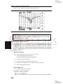
Download Anritsu S113C User`s guide

SgLabs
www.sglabs.it
email: [email protected]
tel. +39 0755149360
Site Master
S113C, S114C,
S331C, and S332C
Antenna, Cable and
Spectrum Analyzer
User's Guide
Hand-Held Tester for Transmission Lines
and other RF Components
Color Front Cover only P/N: 00986-00044
SgLabs
www.sglabs.it
email: [email protected]
tel. +39 0755149360
SgLabs
www.sglabs.it
email: [email protected]
tel. +39 0755149360
SgLabs
www.sglabs.it
email: [email protected]
tel. +39 0755149360
SgLabs
www.sglabs.it
email: [email protected]
tel. +39 0755149360
WARRANTY
The Anritsu product(s) listed on the title page is (are) warranted against defects in
materials and workmanship for one year from the date of shipment.
Anritsu's obligation covers repairing or replacing products which prove to be defective during the warranty period. Buyers shall prepay transportation charges for
equipment returned to Anritsu for warranty repairs. Obligation is limited to the original purchaser. Anritsu is not liable for consequential damages.
LIMITATION OF WARRANTY
The foregoing warranty does not apply to Anritsu connectors that have failed due to
normal wear. Also, the warranty does not apply to defects resulting from improper or
inadequate maintenance by the Buyer, unauthorized modification or misuse, or operation outside the environmental specifications of the product. No other warranty is
expressed or implied, and the remedies provided herein are the Buyer's sole and
exclusive remedies.
TRADEMARK ACKNOWLEDGMENTS
MS-DOS, Windows, Windows 95, Windows NT, Windows 98, Windows 2000, Windows ME and Windows XP are registered trademarks of the Microsoft Corporation.
Anritsu and Site Master are trademarks of Anritsu Company.
NOTICE
Anritsu Company has prepared this manual for use by Anritsu Company personnel
and customers as a guide for the proper installation, operation and maintenance of
Anritsu Company equipment and computer programs. The drawings, specifications,
and information contained herein are the property of Anritsu Company, and any unauthorized use or disclosure of these drawings, specifications, and information is
prohibited; they shall not be reproduced, copied, or used in whole or in part as the
basis for manufacture or sale of the equipment or software programs without the
prior written consent of Anritsu Company.
UPDATES
Updates to this manual, if any, may be downloaded from the Anritsu internet site at:
http://www.us.anritsu.com.
June 2002
Copyright ã 2001-2002 Anritsu Co.
10580-00060
Revision: C
SgLabs
www.sglabs.it
email: [email protected]
tel. +39 0755149360
SgLabs
www.sglabs.it
email: [email protected]
tel. +39 0755149360
SgLabs
www.sglabs.it
email: [email protected]
tel. +39 0755149360
SgLabs
www.sglabs.it
email: [email protected]
tel. +39 0755149360
Table of Contents
Chapter 1 - General Information
Introduction . . . . . . . .
Description . . . . . . . . .
Standard Accessories . . .
Options . . . . . . . . . . .
Printers . . . . . . . . . . .
Optional Accessories. . . .
Performance Specifications
Preventive Maintenance . .
Calibration . . . . . . . . .
InstaCal Module . . . . . .
Annual Verification . . . .
ESD Precautions . . . . . .
.
.
.
.
.
.
.
.
.
.
.
.
.
.
.
.
.
.
.
.
.
.
.
.
.
.
.
.
.
.
.
.
.
.
.
.
.
.
.
.
.
.
.
.
.
.
.
.
.
.
.
.
.
.
.
.
.
.
.
.
.
.
.
.
.
.
.
.
.
.
.
.
.
.
.
.
.
.
.
.
.
.
.
.
.
.
.
.
.
.
.
.
.
.
.
.
.
.
.
.
.
.
.
.
.
.
.
.
.
.
.
.
.
.
.
.
.
.
.
.
.
.
.
.
.
.
.
.
.
.
.
.
.
.
.
.
.
.
.
.
.
.
.
.
.
.
.
.
.
.
.
.
.
.
.
.
.
.
.
.
.
.
.
.
.
.
.
.
.
.
.
.
.
.
.
.
.
.
.
.
.
.
.
.
.
.
.
.
.
.
.
.
.
.
.
.
.
.
.
.
.
.
.
.
.
.
.
.
.
.
.
.
.
.
.
.
.
.
.
.
.
.
.
.
.
.
.
.
.
.
.
.
.
.
.
.
.
.
.
.
.
.
.
.
.
.
.
.
.
.
.
.
.
.
.
.
.
.
.
.
.
.
.
.
.
.
.
.
.
.
.
.
.
.
.
.
.
.
.
.
.
.
.
.
.
.
.
.
.
.
.
.
.
.
.
.
.
.
.
.
.
.
.
.
.
.
.
.
.
.
.
.
1-1
1-1
1-1
1-2
1-2
1-3
1-4
1-6
1-6
1-7
1-7
1-7
Chapter 2 - Functions and Operations
Introduction . . . . . . . . . . . . . . . . . . . . . . . . . . . . . . . . . . 2-1
Test Connector Panel . . . . . . . . . . . . . . . . . . . . . . . . . . . . . 2-1
12.5-15VDC (1100 mA) . . . . . . . . . . . . . . . . . . . . . . . . . 2-1
Battery Charging . . . . . . . . . . . . . . . . . . . . . . . . . . . . . 2-1
External Power . . . . . . . . . . . . . . . . . . . . . . . . . . . . . . 2-1
Serial Interface . . . . . . . . . . . . . . . . . . . . . . . . . . . . . . 2-1
RF Out. . . . . . . . . . . . . . . . . . . . . . . . . . . . . . . . . . . 2-1
RF In . . . . . . . . . . . . . . . . . . . . . . . . . . . . . . . . . . . 2-1
RF Detector . . . . . . . . . . . . . . . . . . . . . . . . . . . . . . . . 2-1
Front Panel Overview . . . . . . . . . . . . . . . . . . . . . . . . . . . . . 2-2
Function Hard Keys . . . . . . . . . . . . . . . . . . . . . . . . . . . . . . 2-3
MODE. . . . . . . . . . . . . . . . . . . . . . . . . . . . . . . . . . . 2-3
FREQ/DIST . . . . . . . . . . . . . . . . . . . . . . . . . . . . . . . . 2-3
AMPLITUDE . . . . . . . . . . . . . . . . . . . . . . . . . . . . . . . 2-3
SWEEP . . . . . . . . . . . . . . . . . . . . . . . . . . . . . . . . . . 2-3
Keypad Hard Keys . . . . . . . . . . . . . . . . . . . . . . . . . . . . . . . 2-4
Soft Keys. . . . . . . . . . . . . . . . . . . . . . . . . . . . . . . . . . . . 2-6
FREQ/DIST . . . . . . . . . . . . . . . . . . . . . . . . . . . . . . . 2-10
Frequency Menu . . . . . . . . . . . . . . . . . . . . . . . . . . . . . 2-10
Distance Menu . . . . . . . . . . . . . . . . . . . . . . . . . . . . . . 2-10
Distance Sub-Menu . . . . . . . . . . . . . . . . . . . . . . . . . . . 2-10
AMPLITUDE . . . . . . . . . . . . . . . . . . . . . . . . . . . . . . 2-12
Amplitude Menu . . . . . . . . . . . . . . . . . . . . . . . . . . . . . 2-12
SWEEP . . . . . . . . . . . . . . . . . . . . . . . . . . . . . . . . . 2-13
Sweep Menu . . . . . . . . . . . . . . . . . . . . . . . . . . . . . . . 2-13
MARKER . . . . . . . . . . . . . . . . . . . . . . . . . . . . . . . . 2-15
LIMIT . . . . . . . . . . . . . . . . . . . . . . . . . . . . . . . . . . 2-16
SYS . . . . . . . . . . . . . . . . . . . . . . . . . . . . . . . . . . . 2-17
Power Monitor Menu . . . . . . . . . . . . . . . . . . . . . . . . . . . . . 2-18
Symbols. . . . . . . . . . . . . . . . . . . . . . . . . . . . . . . . . . . . 2-19
i
SgLabs
www.sglabs.it
email: [email protected]
tel. +39 0755149360
SgLabs
www.sglabs.it
email: [email protected]
tel. +39 0755149360
Self Test . . . . . . . . . . . . . . . . . . . . .
Error Codes . . . . . . . . . . . . . . . . . . . .
Self Test Errors . . . . . . . . . . . . . . . .
Range Errors. . . . . . . . . . . . . . . . . .
InstaCal Error Messages. . . . . . . . . . . .
Battery Information. . . . . . . . . . . . . . . .
Charging a New Battery . . . . . . . . . . . . .
Charging the Battery in the Site Master . . . .
Charging the Battery in the Optional Charger.
Determining Remaining Battery Life. . . . . . .
Battery Life . . . . . . . . . . . . . . . . . .
Important Battery Information . . . . . . . . . .
.
.
.
.
.
.
.
.
.
.
.
.
.
.
.
.
.
.
.
.
.
.
.
.
.
.
.
.
.
.
.
.
.
.
.
.
.
.
.
.
.
.
.
.
.
.
.
.
.
.
.
.
.
.
.
.
.
.
.
.
.
.
.
.
.
.
.
.
.
.
.
.
.
.
.
.
.
.
.
.
.
.
.
.
.
.
.
.
.
.
.
.
.
.
.
.
.
.
.
.
.
.
.
.
.
.
.
.
.
.
.
.
.
.
.
.
.
.
.
.
.
.
.
.
.
.
.
.
.
.
.
.
.
.
.
.
.
.
.
.
.
.
.
.
.
.
.
.
.
.
.
.
.
.
.
.
.
.
.
.
.
.
.
.
.
.
.
.
2-19
2-19
2-19
2-21
2-22
2-24
2-24
2-24
2-24
2-25
2-26
2-27
Chapter 3 - Getting Started
Introduction . . . . . . . . . . . . . . . . . . . . . . . . . . . . . . . . . . 3-1
Power On Procedure . . . . . . . . . . . . . . . . . . . . . . . . . . . . . . 3-1
Site Master Mode . . . . . . . . . . . . . . . . . . . . . . . . . . . . . . . 3-2
Selecting the Frequency or Distance . . . . . . . . . . . . . . . . . . . . 3-2
Calibration . . . . . . . . . . . . . . . . . . . . . . . . . . . . . . . . . 3-2
Calibration Verification. . . . . . . . . . . . . . . . . . . . . . . . . . . 3-3
Manual Calibration Procedure . . . . . . . . . . . . . . . . . . . . . . . 3-4
InstaCal Module Verification. . . . . . . . . . . . . . . . . . . . . . . . 3-5
InstaCal Module Calibration Procedure . . . . . . . . . . . . . . . . . . 3-6
Calibration with the Test Port Extension Cable . . . . . . . . . . . . . . 3-6
Setting the Scale . . . . . . . . . . . . . . . . . . . . . . . . . . . . . . 3-7
Auto Scale . . . . . . . . . . . . . . . . . . . . . . . . . . . . . . . . . 3-7
Amplitude Scale . . . . . . . . . . . . . . . . . . . . . . . . . . . . . . 3-7
Set the Distance and Cable Type . . . . . . . . . . . . . . . . . . . . . . 3-7
Spectrum Analyzer Mode . . . . . . . . . . . . . . . . . . . . . . . . . . . 3-9
Selecting Spectrum Analyzer Mode . . . . . . . . . . . . . . . . . . . . 3-9
Making a Measurement . . . . . . . . . . . . . . . . . . . . . . . . . . . 3-9
Selecting the Frequency . . . . . . . . . . . . . . . . . . . . . . . . . . 3-9
Selecting the Span . . . . . . . . . . . . . . . . . . . . . . . . . . . . . 3-9
Selecting the Amplitude . . . . . . . . . . . . . . . . . . . . . . . . . . 3-9
Selecting Bandwidth Parameters . . . . . . . . . . . . . . . . . . . . . 3-10
Selecting Sweep Parameters. . . . . . . . . . . . . . . . . . . . . . . . 3-10
Adjusting Attenuator Settings . . . . . . . . . . . . . . . . . . . . . . . 3-11
Site Master and Spectrum Analyzer Modes . . . . . . . . . . . . . . . . . 3-12
Save and Recall a Setup . . . . . . . . . . . . . . . . . . . . . . . . . . . 3-12
Saving a Setup . . . . . . . . . . . . . . . . . . . . . . . . . . . . . . . 3-12
Recalling a Setup . . . . . . . . . . . . . . . . . . . . . . . . . . . . . 3-12
Save and Recall a Display . . . . . . . . . . . . . . . . . . . . . . . . . . 3-12
Saving a Display. . . . . . . . . . . . . . . . . . . . . . . . . . . . . . 3-12
Recalling a Display . . . . . . . . . . . . . . . . . . . . . . . . . . . . 3-12
Changing the Units . . . . . . . . . . . . . . . . . . . . . . . . . . . . . . 3-13
Changing the Display Language . . . . . . . . . . . . . . . . . . . . . . . 3-13
Adjusting Markers . . . . . . . . . . . . . . . . . . . . . . . . . . . . . . 3-13
ii
SgLabs
www.sglabs.it
email: [email protected]
tel. +39 0755149360
SgLabs
www.sglabs.it
email: [email protected]
tel. +39 0755149360
Adjusting Limits . . . . . . . . . . . . . . . . . . . . . . . . . . . . . . . 3-13
Adjusting the Display Contrast . . . . . . . . . . . . . . . . . . . . . . . . 3-15
Setting the System Language . . . . . . . . . . . . . . . . . . . . . . . . . 3-15
Setting the System Impedance
Printing . . . . . . . . . . . .
Printing a Screen . . . . .
Printer Switch Settings . .
Using the Soft Carrying Case.
.
.
.
.
.
.
.
.
.
.
.
.
.
.
.
.
.
.
.
.
.
.
.
.
.
.
.
.
.
.
.
.
.
.
.
.
.
.
.
.
.
.
.
.
.
.
.
.
.
.
.
.
.
.
.
.
.
.
.
.
.
.
.
.
.
.
.
.
.
.
.
.
.
.
.
.
.
.
.
.
.
.
.
.
.
.
.
.
.
.
.
.
.
.
.
.
.
.
.
.
.
.
.
.
.
.
.
.
.
.
.
.
.
.
.
.
.
.
.
.
3-15
3-16
3-16
3-17
3-18
Chapter 4 - Cable & Antenna Measurements
Introduction . . . . . . . . . . . . . . . . . . . . . . . . . . . . . . . . . . 4-1
Line Sweep Fundamentals . . . . . . . . . . . . . . . . . . . . . . . . . . . 4-1
Information Required for a Line Sweep . . . . . . . . . . . . . . . . . . . . 4-2
Typical Line Sweep Test Procedures . . . . . . . . . . . . . . . . . . . . . 4-3
System Return Loss Measurement . . . . . . . . . . . . . . . . . . . . . 4-3
Insertion Loss Measurement . . . . . . . . . . . . . . . . . . . . . . . . 4-4
Distance-To-Fault (DTF) Transmission Line Test . . . . . . . . . . . . . 4-8
Resolution. . . . . . . . . . . . . . . . . . . . . . . . . . . . . . . . . . 4-9
Antenna Subsystem Return Loss Test. . . . . . . . . . . . . . . . . . . 4-10
Chapter 5 - Spectrum Analyzer Measurements
Spectrum Analyzer Fundamentals . . . .
Site Master Spectrum Analyzer Features
AM/FM Modulation . . . . . . . . . . .
Amplitude Modulation . . . . . . . .
Frequency Modulation . . . . . . . .
Field Strength Measurements . . . . . .
.
.
.
.
.
.
.
.
.
.
.
.
.
.
.
.
.
.
.
.
.
.
.
.
.
.
.
.
.
.
.
.
.
.
.
.
.
.
.
.
.
.
.
.
.
.
.
.
.
.
.
.
.
.
.
.
.
.
.
.
.
.
.
.
.
.
.
.
.
.
.
.
.
.
.
.
.
.
.
.
.
.
.
.
.
.
.
.
.
.
.
.
.
.
.
.
.
.
.
.
.
.
.
.
.
.
.
.
.
.
.
.
.
.
5-1
5-3
5-3
5-3
5-4
5-6
Creating a Spectral Mask . . . . . . . . . . . . . . . . . . . . . . . . . . . 5-7
Trace Overlay . . . . . . . . . . . . . . . . . . . . . . . . . . . . . . . . . 5-9
Occupied Bandwidth . . . . . . . . . . . . . . . . . . . . . . . . . . . . . 5-10
Percent of Power Method . . . . . . . . . . . . . . . . . . . . . . . . . 5-10
XdB Down Method . . . . . . . . . . . . . . . . . . . . . . . . . . . . 5-10
Required Equipment. . . . . . . . . . . . . . . . . . . . . . . . . . . . 5-10
Procedure . . . . . . . . . . . . . . . . . . . . . . . . . . . . . . . . . 5-10
Channel Power Measurement . . . . . . . . . . . . . . . . . . . . . . . . 5-12
GSM Channel Power Measurement . . . . . . . . . . . . . . . . . . . . . 5-12
Required Equipment. . . . . . . . . . . . . . . . . . . . . . . . . . . . 5-12
Procedure . . . . . . . . . . . . . . . . . . . . . . . . . . . . . . . . . 5-13
Adjacent Channel Power Ratio . . . . . . . . . . . . . . . . . . . . . . . . 5-15
GSM Adjacent Channel Power Measurement . . . . . . . . . . . . . . . . 5-15
Required Equipment. . . . . . . . . . . . . . . . . . . . . . . . . . . . 5-15
Procedure . . . . . . . . . . . . . . . . . . . . . . . . . . . . . . . . . 5-15
Measurement Applications . . . . . . . . . . . . . . . . . . . . . . . . . . 5-17
Resolving Closely Spaced Signals . . . . . . . . . . . . . . . . . . . . . . 5-17
Measurement of Two Signals Having Equal Amplitudes . . . . . . . . 5-17
Measurement of Two Signals Having Unequal Amplitudes . . . . . . . 5-19
iii
SgLabs
www.sglabs.it
email: [email protected]
tel. +39 0755149360
SgLabs
www.sglabs.it
email: [email protected]
tel. +39 0755149360
Out-of-Band Spurious Emissions. . . . . . . . . . . . . . . . . . . . . . . 5-23
Out-of-Band Spurious Emission Measurement
Required Equipment. . . . . . . . . . . . .
Procedure . . . . . . . . . . . . . . . . . .
In-band/Out-of-Channel Measurements . . . .
In-band Spurious Measurement . . . . . . .
Required Equipment. . . . . . . . . . . . .
Procedure . . . . . . . . . . . . . . . . . .
Field Strength . . . . . . . . . . . . . . . . . .
Required Equipment. . . . . . . . . . . . .
Procedure . . . . . . . . . . . . . . . . . .
Antenna Calculations . . . . . . . . . . . .
.
.
.
.
.
.
.
.
.
.
.
.
.
.
.
.
.
.
.
.
.
.
.
.
.
.
.
.
.
.
.
.
.
.
.
.
.
.
.
.
.
.
.
.
.
.
.
.
.
.
.
.
.
.
.
.
.
.
.
.
.
.
.
.
.
.
.
.
.
.
.
.
.
.
.
.
.
.
.
.
.
.
.
.
.
.
.
.
.
.
.
.
.
.
.
.
.
.
.
.
.
.
.
.
.
.
.
.
.
.
.
.
.
.
.
.
.
.
.
.
.
.
.
.
.
.
.
.
.
.
.
.
.
.
.
.
.
.
.
.
.
.
.
.
.
.
.
.
.
.
.
.
.
.
.
.
.
.
.
.
.
.
.
.
.
5-23
5-23
5-23
5-25
5-25
5-25
5-25
5-27
5-27
5-27
5-28
Chapter 6 - Power Measurement
Introduction . . . . . . . . . . . . . . . . . . . . . . . . . . . . . . . . . . 6-1
Power Measurement . . . . . . . . . . . . . . . . . . . . . . . . . . . . . . 6-1
Chapter 7 - Software Tools
Introduction . . . . . . . . . .
Features . . . . . . . . . . . .
System Requirements . . . . .
Installation . . . . . . . . . . .
Communication Port Setting
Interface Cable Installation .
Using Software Tools . . . . .
Downloading Traces . . . . . .
.
.
.
.
.
.
.
.
.
.
.
.
.
.
.
.
.
.
.
.
.
.
.
.
.
.
.
.
.
.
.
.
.
.
.
.
.
.
.
.
.
.
.
.
.
.
.
.
.
.
.
.
.
.
.
.
.
.
.
.
.
.
.
.
.
.
.
.
.
.
.
.
.
.
.
.
.
.
.
.
.
.
.
.
.
.
.
.
.
.
.
.
.
.
.
.
.
.
.
.
.
.
.
.
.
.
.
.
.
.
.
.
.
.
.
.
.
.
.
.
.
.
.
.
.
.
.
.
.
.
.
.
.
.
.
.
.
.
.
.
.
.
.
.
.
.
.
.
.
.
.
.
.
.
.
.
.
.
.
.
.
.
.
.
.
.
.
.
.
.
.
.
.
.
.
.
.
.
.
.
.
.
.
.
.
.
.
.
.
.
.
.
7-1
7-1
7-1
7-2
7-2
7-3
7-3
7-3
Plot Capture to the PC . . . . . . . . . . . . . .
Plot Upload to the Instrument . . . . . . . . . .
Plot Properties . . . . . . . . . . . . . . . . . .
Trace Overlay or Plot Overlay . . . . . . . .
Saving Traces . . . . . . . . . . . . . . . . .
Creating a Database. . . . . . . . . . . . . .
Printing Formats . . . . . . . . . . . . . . .
Entering Antenna Factors in Software Tools .
Uploading Antenna Factors. . . . . . . . . .
Downloading Antennas . . . . . . . . . . . .
.
.
.
.
.
.
.
.
.
.
.
.
.
.
.
.
.
.
.
.
.
.
.
.
.
.
.
.
.
.
.
.
.
.
.
.
.
.
.
.
.
.
.
.
.
.
.
.
.
.
.
.
.
.
.
.
.
.
.
.
.
.
.
.
.
.
.
.
.
.
.
.
.
.
.
.
.
.
.
.
.
.
.
.
.
.
.
.
.
.
.
.
.
.
.
.
.
.
.
.
.
.
.
.
.
.
.
.
.
.
.
.
.
.
.
.
.
.
.
.
.
.
.
.
.
.
.
.
.
.
.
.
.
.
.
.
.
.
.
.
.
.
.
.
.
.
.
.
.
.
7-4
7-4
7-4
7-5
7-6
7-7
7-7
7-7
7-8
7-9
Appendix A - Reference Data
Coaxial Cable Technical Data. . . . . . . . . . . . . . . . . . . . . . . . . A-1
Appendix B - Windowing
Introduction . . . . . . . . . . . . . . . . . . . . . . . . . . . . . . . . . . B-1
Examples . . . . . . . . . . . . . . . . . . . . . . . . . . . . . . . . . . . B-1
iv
SgLabs
www.sglabs.it
email: [email protected]
tel. +39 0755149360
SgLabs
www.sglabs.it
email: [email protected]
tel. +39 0755149360
Chapter 1
General Information
Introduction
This chapter provides a description, performance specifications, optional accessories, preventive maintenance, and calibration requirements for the Site Master models S113C,
S114C, S331C, and S332C. Throughout this manual, the term Site Master will refer to the
models S113C, S114C, S331C, and S332C.
Model
S113C
S114C
S331C
S332C
1
Frequency Range
2 to 1600 MHz
2 to 1600 MHz, 100 kHz to 1600 MHz Spectrum Analysis
25 to 4000 MHz
25 to 4000 MHz, 100 kHz to 3000 MHz Spectrum Analysis
Description
The Site Master is a hand held SWR/RL (standing wave ratio/return loss), and Distance-ToFault (DTF) measurement instrument that includes a built-in synthesized signal source. All
models include a keypad to enter data and a liquid crystal display (LCD) to provide graphic
indications of SWR or RL over the selected frequency range and selected distance. The Site
Master is capable of up to 2.5 hours of continuous operation from a fully charged
field-replaceable battery and can be operated from a 12.5 dc source. Built-in energy conservation features can be used to extend battery life over an eight-hour work day.
The Site Master is designed for measuring SWR, return loss, or cable insertion loss and locating faulty RF components in antenna systems. Power monitoring is available as an option. Site Master models S114C and S332C include spectrum analysis capability. The
displayed trace can be scaled or enhanced with frequency markers or limit lines. A menu
option provides for an audible “beep” when the limit value is exceeded. To permit use in
low-light environments, the LCD can be back lit using a front panel key.
Standard Accessories
The Software Tools PC-based software program provides a database record for storing
measurement data. Site Master Software Tools can also convert the Site Master display to a
Microsoft Windowsä 95/98/NT4/2000/ME/XP workstation graphic. Measurements stored
in the Site Master internal memory can be downloaded to the PC using the included
null-modem serial cable. Once stored, the graphic trace can be displayed, scaled, or enhanced with markers and limit lines. Historical graphs can be overlaid with current data,
and underlying data can be extracted and used in spreadsheets or for other analytical tasks.
The Site Master Software Tools program can display all of the measurements made with the
Site Master (SWR, return loss, cable loss, distance-to-fault) as well as providing other functions, such as converting display modes and Smith charts. Refer to Chapter 7, Software
Tools, for more information.
1-1
SgLabs
www.sglabs.it
email: [email protected]
tel. +39 0755149360
SgLabs
www.sglabs.it
email: [email protected]
tel. +39 0755149360
Chapter 1 General Information
The following items are supplied with the basic hardware.
·
Soft Carrying Case
·
AC-DC Adapter
·
Automotive Cigarette Lighter 12 Volt DC Adapter,
·
CDROM disk containing the Software Tools program. This program contains Fault Location (DTF) and Smith Chart functions
·
Serial Interface Cable (null modem type)
·
One year Warranty (includes battery, firmware, and software)
·
User's Guide
Options
·
Option 5 — Add Power Monitor
·
RF Detector, 1 to 3000 MHz, N(m) input connector, 50 Ohms, Part No. 5400-71N50
·
RF Detector, 0.01 to 20 GHz, N(m) input connector, 50 Ohms, Part No. 560-7N50B
Printers
·
2000-766
HP DeskJet Printer, with Interface Cable, Black Print Cartridge,
and U.S. Power Cable
·
2000-1206
Black Print Cartrige for HP350 DeskJet
·
2000-1207
Rechargeable Battery Pack for HP 350 DeskJet
·
2000-753
Serial-to-Parallel Converter Cable
·
2000-663
Power Cable (Europe) for DeskJet Printer
·
2000-664
Power Cable (Australia) for DeskJet Printer
·
2000-665
Power Cable (U.K.) for DeskJet Printer
·
2000-667
Power Cable (So. Africa) for DeskJet Printer
·
2000-1008
Sieko DPU-414-30BU Thermal Printer with Internal
Battery, Thermal Printer Paper, Serial Cable, Power Cable
·
2000-755
Five rolls of Thermal Paper
·
2000-1002
U.S. Adapter for Seiko DPU-414-30B
·
2000-1003
Euro Adapter for Seiko DPU-414-30B
·
2000-1194
Japan Adapter for Seiko DPU-414-30B
·
2000-1004
Battery Pack Adapter for Seiko DPU-414-30B
·
2000-1012
Serial 9-pin male to 9-pin female cable for Seiko DPU-414-30B
·
2000-1046
Serial-to-parallel Converter Cable w/ DIP switch labeling, 36-pin
female Centronics to DB25 female
1-2
SgLabs
www.sglabs.it
email: [email protected]
tel. +39 0755149360
SgLabs
www.sglabs.it
email: [email protected]
tel. +39 0755149360
Chapter 1
General Information
Optional Accessories
Part Number
Description
10580-00061
S113C, S114C, S331C, S332C Programming Manual (on disk only)
10580-00062
S113C/S331C Maintenance Manual
10580-00068
S114C/S332C Maintenance Manual
760-215A
Transit Case for Site Master
633-27
Rechargeable Battery, NiMH
2000-1029
Battery Charger with universal power supply, NiMH only
48258
Soft Carrying Case
40-115
AC Adaptor Power Supply
806-62
Cable Assy, Cig Plug, Female
800-441
Serial Interface Cable Assy
551-1691
USB Adapter Cable
2300-347
Software Tools CD
ICN50
InstaCal™ Calibration Module, 50 Ohm, 2 MHz to 4.0 GHz, N (m)
OSLN50LF
Anritsu Precision N (m) Open/Short/Load, 42 dB
OSLNF50LF
Anritsu Precision N (f) Open/Short/Load, 42 dB
22N50
Anritsu Precision N (m) Short/Open
22NF50
Anritsu Precision N (f) Short/Open
SM/PL
Site Master Precision N (m) Load, 42 dB
SM/PLNF
Site Master Precision N (f) Load, 42 dB
2000-767
7/16 (m) Precision Open/Short/Load
2000-768
7/16 (f) Precision Open/Short/Load
34NN50A
Adapter, Precision N (m) to N (m)
34NFNF50
Adapter, Precision N (f) to N (f)
510-90
Adapter, 7/16 (f) to N (m)
510-91
Adapter, 7/16 (f) to N (f)
510-92
Adapter, 7/16 (m) to N (m)
510-93
Adapter, 7/16 (m) to N (f)
510-96
Adapter, 7/16 DIN (m) to 7/16 DIN (m)
510-97
Adapter, 7/16 DIN (f) to 7/16 DIN (f)
15NNF50-1.5C
Armored Test Port Extension Cable, 1.5 meter, N (m) to N (f)
15NNF50-3.0C
Armored Test Port Extension Cable, 3.0 meter, N (m) to N (f)
15NNF50-5.0C
Armored Test Port Extension Cable, 5.0 meter, N (m) to N (f)
15NN50-1.5C
Armored Test Port Extension Cable, 1.5 meter, N (m) to N (m)
15NN50-3.0C
Armored Test Port Extension Cable, 3.0 meter, N (m) to N (m)
15NN50-5.0C
Armored Test Port Extension Cable, 5.0 meter, N (m) to N (m)
15NDF50-1.5C
Armored Test Port Extension Cable, 1.5 meter, N (m) to 7/16 DIN (f)
15ND50-1.5C
Armored Test Port Extension Cable, 1.5 meter, N (m) to 7/16 DIN (m)
12N50-75B
Matching Pad, converts 75 W to 50 W, 7.5 dB loss, DC to 3,000 MHz, 50 W
N(m) to 75 W N(f)
2000-1030
Antenna SMA (m), 50 W, 1.71 to 1.88 GHz
2000-1031
Antenna SMA (m), 50 W, 1.85 to 1.99 GHz
2000-1032
Antenna SMA (m), 50 W, 2.4 to 2.5 GHz
2000-1035
Antenna SMA (m), 50 W, 896 to 941 MHz
2000-1200
Antenna SMA (m), 50 W, 806-869MHz
1-3
SgLabs
www.sglabs.it
email: [email protected]
tel. +39 0755149360
SgLabs
www.sglabs.it
email: [email protected]
tel. +39 0755149360
Chapter 1 General Information
Performance Specifications
Performance specifications are provided in Table 1-1, on the following page.
Table 1-1.
Performance Specifications (1 of 2)
Specifications are valid when the unit is calibrated at ambient temperature after a five minute
warmup. Typical values are provided for reference only and are not guaranteed.
Description
Site Master:
S113C, S114C
S331C, S332C
Frequency Accuracy (RF Source Mode)
Frequency Resolution: S113C, S114C
S331C, S332C
SWR:
Range
Resolution
Return Loss:
Range
Resolution
**Distance-To-Fault (DTF):
Vertical Range
Return Loss:
SWR:
Horizontal Range
Value
Frequency Range:
2 to 1600 MHz
25 to 4000 MHz
£75 parts per million @ 25°C*
10 kHz
100 kHz
1.00 to 65.00
0.01
0.00 to 54.00 dB
0.01 dB
0.00 to 54.00 dB
1.00 to 65.00
0 to ((# of data points –1) ´ resolution) a maximum
of 1000m (3281 ft.) with a maximum of 517 points
resolution, # of data pts. = 130, 259, 517
Horizontal Resolution for Coax
(rectangular windowing)
(1.5 ´ 108)(Vp)
DF
Where Vp is the relative propagation velocity of
the cable; dp is the number of data points
(130, 259, 517); DF is the stop frequency minus the
start frequency (Hz)
Horizontal Resolution for Waveguide
1.5 ´ 108 ( 1- (Fc / F1)2)
DF
Where FC is the waveguide cutoff frequency (Hz);
F1 is the start frequency (Hz); DF is the stop frequency minus the start frequency (Hz)
RF Power Monitor:
Display Range
–80.0 to +80 dBm or
10.0 pW to 100.0 kW
–50 dBm to +20 dBm, or 10 mW to 100 mW
0 to +60.0 dB
0.1 dB or 0.1 W
Type N, 50W, female
on-channel
on-frequency
+17 dBm
+10 dBm
+17 dBm
–6 dBm
Detector Range
Offset Range
Resolution
Test Port Connector
***Immunity to Interfering signals
up to the level of: S113C, S114C
S331C, S332C
Maximum Input without Damage:
Test Port, Type N (f)
+20 dBm, 50W, +50 VDC
RF Power Detector
+20 dBm, 50W, +50 VDC
Measurement Accuracy:
Measurement accuracy depends on calibration components. Precision calibration components
have a directivity of 42 dB.
Cable Insertion Loss:
Range
0.00 to 54.00 dB
Resolution
0.01 dB
1-4
SgLabs
www.sglabs.it
email: [email protected]
tel. +39 0755149360
SgLabs
www.sglabs.it
email: [email protected]
tel. +39 0755149360
Chapter 1
Table 1-2.
General Information
Performance Specifications (2 of 2)
Transmission Line Loss (one-port)
Range
Resolution
Spectrum Analyzer:
Frequency Range
S114C
S332C
Frequency Reference
Aging
Accuracy
Frequency Span
S114C
S332C
Sweep Time
0.00 to 20.00 dB
0.01 dB
100 kHz to 1.6 GHz
100 kHz to 3.0 GHz
±1 ppm/yr
±2 ppm
0 Hz (zero span) 100 kHz to 1.6 GHz
0 Hz (zero span) 100 kHz to 3.0 GHz
³6500 ms (full span)
500 ms (zero span)
Resolution Bandwidth
10 kHz, 30 kHz, 100 kHz, 1 MHz
Accuracy
± 20% typical
Video Bandwidth
100 Hz to 300 kHz in 1-3 sequence
SSB Phase Noise (1 GHz) @ 30 kHz offset £ –75 dBc/Hz
Spurious Responses, Input Related
£ –45 dBc
Spurious Residual Responses
£ 90 dBm @ ³ 500 kHz
Note: 10 kHz resolution bandwidth, input terminated, no attenuation
Amplitude
Measurement Range
–95 dBm to +20 dBm typical
Dynamic Range
³ 65 dB typical
Maximum Safe Input Level
+20 dBm, maximum measurable safe input
+23 dBm, maximum input (damage)
+23 dBm, peak pulse power
±50 Vdc
Displayed Average Noise Level:
£ –80 dBm (<500 kHz typical)
£ –95 dBm (³500 kHz typical)
Display Range, Log Scale
2 to 15 dB/div. in 1 dB steps; 10 divisions displayed.
Frequency Response
RF Input VSWR
2.0:1
Resolution (Ref. Level)
1.0 dB
Total Level Accuracy****
±2 dB ³ 500 kHz typical
±3 dB <500 kHz typical
General
Internal Memory:
Trace Memory
200 maximum
Instrument Configuration
10 setup locations
RS-232
9 pin D-sub, three wire serial
Electromagnetic Compatibility
Complies with European community requirements
for CE marking
External DC Input
+11 to +15 Vdc, 1250 mA max.
Temperature: Storage
–20° C to 75° C
Operating
0° C to 50° C
Weight:
2.15 kg (4.76 pounds)
Dimensions:
25.4 x 17.8 x 6.1 cm
(10 x 7 x 2.4 inches)
* ±2 ppm/D°C from 25°C;
** Fault location is accomplished by inverse Fourier Transformation of data taken with the Site Master. Resolution and
maximum range depend on the number of frequency data points, frequency sweep range and relative propagation velocity
of the cable being tested.;
*** Immunity measurement is made in CW mode with incoming interfering signal exactly at the same frequency (worst
case situation). Typical immunity is better when swept frequency is used.;
**** For input signal levels ³ –60 dBm, accuracy at 50 MHz @ –30 dBm = ± 1dB.
1-5
SgLabs
www.sglabs.it
email: [email protected]
tel. +39 0755149360
SgLabs
www.sglabs.it
email: [email protected]
tel. +39 0755149360
Chapter 1 General Information
Preventive Maintenance
Site Master preventive maintenance consists of cleaning the unit and inspecting and cleaning the RF connectors on the instrument and all accessories.
Clean the Site Master with a soft, lint-free cloth dampened with water or water and a mild
cleaning solution.
CAUTION: To avoid damaging the display or case, do not use solvents or abrasive cleaners.
Clean the RF connectors and center pins with a cotton swab dampened with denatured alcohol. Visually inspect the connectors. The fingers of the N (f) connectors and the pins of the
N (m) connectors should be unbroken and uniform in appearance. If you are unsure whether
the connectors are good, gauge the connectors to confirm that the dimensions are correct.
Visually inspect the test port cable(s). The test port cable should be uniform in appearance,
not stretched, kinked, dented, or broken.
Calibration
The Site Master is a field portable unit operating in the rigors of the test environment. An
Open-Short-Load (OSL) calibration should be performed prior to making a measurement in
the field (see Calibration, page 3-2). A built-in temperature sensor in the Site Master advises the user, via an icon located on the right side of the LCD screen, that the internal temperature has exceeded a safety window, and the user is advised to perform another OSL
calibration in order to maintain the integrity of the measurement.
NOTES:
For best calibration results—compensation for all measurement uncertainties—ensure that the Open/Short/Load is at the end of the test port or optional
extension cable; that is, at the same point that you will connect the antenna or
device to be tested.
For best results, use a phase stable Test Port Extension Cable (see Optional
Accessories). If you use a typical laboratory cable to extend the Site Master test
port to the device under test, cable bending subsequent to the OSL calibration
will cause uncompensated phase reflections inside the cable. Thus, cables
which are NOT phase stable may cause measurement errors that are more pronounced as the test frequency increases.
For optimum calibration, Anritsu recommends using precision calibration components.
1-6
SgLabs
www.sglabs.it
email: [email protected]
tel. +39 0755149360
SgLabs
www.sglabs.it
email: [email protected]
tel. +39 0755149360
Chapter 1
General Information
InstaCal Module
The Anritsu InstaCal module can be used in place of discrete components to calibrate the
Site Master. The InstaCal module can be used to perform an Open, Short and Load (OSL)
calibration procedure. Calibration of the Site Master with the InstaCal takes approximately
45 seconds (see Calibration, page 3-2). Unlike a discrete calibration component, the
InstaCal module can not be used at the top of the tower to conduct load or insertion loss
measurements. The module operates from 2 MHz to 4 GHz and weighs eight ounces.
Anritsu recommends annual verification of the InstaCal module to verify performance with
precision instrument data. The verification may be performed at a local Anritsu Service
Center or at the Anritsu factory.
Annual Verification
Anritsu recommends an annual calibration and performance verification of the Site Master
and the OSL calibration components and InstaCal module by local Anritsu service centers.
Anritsu service centers are listed in Table 1-2 on the following page.
The Site Master itself is self-calibrating, meaning that there are no field-adjustable components. However, the OSL calibration components are crucial to the integrity of the calibration and therefore, must be verified periodically to ensure performance conformity. This is
especially important if the OSL calibration components have been accidentally dropped or
over-torqued.
ESD Precautions
The Site Master, like other high performance instruments, is susceptible to ESD damage.
Very often, coaxial cables and antennas build up a static charge, which, if allowed to discharge by connecting to the Site Master, may damage the Site Master input circuitry. Site
Master operators should be aware of the potential for ESD damage and take all necessary
precautions. Operators should exercise practices outlined within industry standards like
JEDEC-625 (EIA-625), MIL-HDBK-263, and MIL-STD-1686, which pertain to ESD and
ESDS devices, equipment, and practices.
As these apply to the Site Master, it is recommended to dissipate any static charges that
may be present before connecting the coaxial cables or antennas to the Site Master. This
may be as simple as temporarily attaching a short or load device to the cable or antenna
prior to attaching to the Site Master. It is important to remember that the operator may also
carry a static charge that can cause damage. Following the practices outlined in the above
standards will insure a safe environment for both personnel and equipment.
1-7
SgLabs
www.sglabs.it
email: [email protected]
tel. +39 0755149360
SgLabs
www.sglabs.it
email: [email protected]
tel. +39 0755149360
Chapter 1 General Information
Table 1-2.
Anritsu Service Centers
UNITED STATES
GERMANY
SOUTH AFRICA
ANRITSU COMPANY
685 Jarvis Drive
Morgan Hill, CA 95037-2809
Telephone: (408) 776-8300
FAX: 408-776-1744
ANRITSU GmbH
Grafenberger Allee 54-56
D-40237 Dusseldorf
Germany
Telephone: 0211-968550
FAX: 0211-9685555
ETESCSA
12 Surrey Square Office Park
330 Surrey Avenue
Ferndale, Randburt, 2194
South Africa
Telephone: 011-27-11-787-7200
Fax: 011-27-11-787-0446
ANRITSU COMPANY
10 NewMaple Ave., Suite 305
Pine Brook, NJ 07058
Telephone: 973-227-8999
FAX: 973-575-0092
ANRITSU COMPANY
1155 E. Collins Blvd
Richardson, TX 75081
Telephone: 1-800-ANRITSU
FAX: 972-671-1877
AUSTRALIA
ANRITSU PTY. LTD.
Unit 3, 170 Foster Road
Mt Waverley, VIC 3149
Australia
Telephone: 03-9558-8177
FAX: 03-9558-8255
BRAZIL
ANRITSU ELECTRONICA LTDA.
Praia de Botafogo 440. Sala 2401
CEP22250-040,Rio de Janeiro,RJ,
Brasil
Telephone: 021-527-6922
FAX: 021-53-71-456
CANADA
ANRITSU INSTRUMENTS LTD.
700 Silver Seven Road, Suite 120
Kanata, Ontario K2V 1C3
Telephone: (613) 591-2003
FAX: (613) 591-1006
CHINA (SHANGHAI)
ANRITSU ELECTRONICS CO LTD
2F,Rm.B, 52 Section Factory Bldg.
NO 516 Fu Te Road (N)
Waigaoqiao Free Trade Zone
Pudong, Shanghai 200131
PR CHINA
Telephone: 86-21-58680226
FAX: 86-21-58680588
FRANCE
ANRITSU S.A
9 Avenue du Quebec
Zone de Courtaboeuf
91951 Les Ulis Cedex
Telephone: 016-09-21-550
FAX: 016-44-61-065
INDIA
MEERA AGENCIES (P) LTD
A-23 Hauz Khas
New Delhi, India 110 016
Telephone: 011-685-3959
FAX: 011-686-6720
ISRAEL
TECH-CENT, LTD
4 Raul Valenberg St.
Tel-Aviv, Israel 69719
Telephone: 972-36-478563
FAX: 972-36-478334
ITALY
ANRITSU Sp.A
Rome Office
Via E. Vittorini, 129
00144 Roma EUR
Telephone: (06) 50-2299-711
FAX: 06-50-22-4252
JAPAN
ANRITSU CUSTOMER SERVICE LTD.
1800 Onna Atsugi—shi
Kanagawa-Prf. 243 Japan
Telephone: 0462-96-6688
FAX: 0462-25-8379
SWEDEN
ANRITSU AB
Botvid Center
Fittja Backe 13A
145 84
Stockholm, Sweden
Telephone: (08) 534-707-00
FAX: (08)534-707-30
TAIWAN
ANRITSU CO., LTD.
6F, No. 96, Section 3
Chien Kuo N. Road
Taipei, Taiwan, R.O.C.
Telephone: (02) 515-6050
FAX: (02) 509-5519
UNITED KINGDOM
ANRITSU LTD.
200 Capability Green
Luton, Bedfordshire
LU1 3LU, England
Telephone: 015-82-43-3200
FAX: 015-82-73-1303
KOREA
ANRITSU SERVICE CENTER
8F Sanwon Bldg.
1329-8 Seocho-Dong
Seocho-Ku
Seoul, Korea 137-070
Telephone: 82-2-581-6603
FAX: 82-2-582-6603
SINGAPORE
ANRITSU (SINGAPORE) PTE LTD
10, Hoe Chiang Road
#07-01/02
Keppel Towers
Singapore 089315
Telephone:65-282-2400
FAX:65-282-2533
1-8
SgLabs
www.sglabs.it
email: [email protected]
tel. +39 0755149360
SgLabs
www.sglabs.it
email: [email protected]
tel. +39 0755149360
Chapter 2
Functions and Operations
Introduction
This chapter provides a brief overview of the Site Master functions and operations, providing the user with a starting point for making basic measurements. For more detailed information, refer to Chapter 4, Cable & Antenna Measurements, Chapter 5, Spectrum Analyzer
Measurements, and Chapter 7, Software Tools.
The Site Master is designed specifically for field environments and applications requiring
mobility. As such, it is a lightweight, handheld, battery operated unit which can be easily
carried to any location, and is capable of up to 2.5 hours of continuous operation from a
fully charged battery. Built-in energy conservation features allow battery life to be extended
over an eight-hour workday. The Site Master can also be powered by a 12.5 Vdc external
source. The external source can be either the Anritsu AC-DC Adapter (P/N 40-115) or 12.5
Vdc Automotive Cigarette Lighter Adapter (P/N 806-62). Both items are standard accessories.
2
Test Connector Panel
The connectors and indicators located on the test panel (Figure 2-1) are listed and described
below.
12.5-15VDC
(1100 mA)
12.5 to 15 Vdc @ 1100 mA input to power the unit or for battery charging.
WARNING
When using the AC-DC Adapter, always use a three-wire power cable connected
to a three-wire power line outlet. If power is supplied without grounding the equipment in this manner, there is a risk of receiving a severe or fatal electric shock.
Battery
Charging
Illuminates when the battery is being charged. The indicator automatically shuts
off when the battery is fully charged.
External
Power
Illuminates when the Site Master is being powered by the external charging unit.
Serial
Interface
RS232 DB9 interface to a COM port on a personal computer (for use with the
Anritsu Software Tools program) or to a supported printer.
RF Out
RF output, 50 W impedance, for reflection measurements.
RF In
RF input, 50 W impedance, for spectrum analysis measurements.
RF Detector
RF detector input for the Power Monitor.
2-1
SgLabs
www.sglabs.it
email: [email protected]
tel. +39 0755149360
SgLabs
www.sglabs.it
email: [email protected]
tel. +39 0755149360
Chapter 2 Functions and Operations
SERIAL INTERFACE
EXTERNAL POWER LED
EXTERNAL POWER
RF DETECTOR
BATTERY
CHARGING
LED
RF IN
RF OUT
Figure 2-1.
Test Connector Panel
Front Panel Overview
The Site Master menu-driven user interface is easy to use and requires little training. Hard
keys on the front panel are used to initiate function-specific menus. There are four function
hard keys located below the display, Mode, Frequency/Distance, Amplitude and Sweep.
There are seventeen keypad hard keys located to the right of the display. Twelve of the keypad hard keys perform more than one function, depending on the current mode of operation.
The dual purpose keys are labeled with one function in black, the other in blue.
There are also six soft keys that change function depending upon the current mode selection. The current soft key function is indicated in the active function block to the right of
the display. The locations of the different keys are illustrated in Figure 2-2.
Active
Function
Block
Soft Keys
Site Master S332C
1
2
START
CAL
AUTO
SCALE
SAVE
SETUP
RECALL
SETUP
3
5
LIMIT
7
SAVE
DISPLAY
9
ON
OFF
MODE
FREQ/DIST
AMPLITUDE
ESCAPE
CLEAR
4
6
MARKER
8
RECALL
DISPLAY
0
ENTER
Keypad
Hard
Keys
RUN
HOLD
+/-
PRINT
.
SYS
SWEEP
Function Hard Keys
Figure 2-2.
Site Master Soft Keys
The following sections describe the various key functions.
2-2
SgLabs
www.sglabs.it
email: [email protected]
tel. +39 0755149360
SgLabs
www.sglabs.it
email: [email protected]
tel. +39 0755149360
Chapter 2 Functions and Operations
Function Hard Keys
MODE
Opens the mode selection box (below). Use the Up/Down arrow key to select a
mode. Press the ENTER key to implement.
MEASUREMENT MODE
FREQ -
SWR
RETURN LOSS
CABLE LOSS - ONE PORT
DTF -
SWR
RETURN LOSS
POWER MONITOR
SPECTRUM ANALYZER
Figure 2-3.
Mode Selection Box
FREQ/DIST
Displays the Frequency or Distance to Fault softkey menus depending on the
measurement mode.
AMPLITUDE
Displays the amplitude softkey menu for the current operating mode.
SWEEP
Displays the Sweep function softkey menu for the current operating mode.
2-3
SgLabs
www.sglabs.it
email: [email protected]
tel. +39 0755149360
SgLabs
www.sglabs.it
email: [email protected]
tel. +39 0755149360
Chapter 2 Functions and Operations
Keypad Hard Keys
This section contains an alphabetical listing of the Site Master front panel keypad controls
along with a brief description of each. More detailed descriptions of the major function
keys follow.
The following keypad hard key functions are printed in black on the keypad keys.
0-9
These keys are used to enter numerical data as required to setup or perform measurements.
+/–
The plus/minus key is used to enter positive or negative values as required
to setup or perform measurements.
·
The decimal point is used to enter decimal values as required to setup or
perform measurements.
ESCAPE
CLEAR
Exits the present operation or clears the display. If a parameter is being
edited, pressing this key will clear the value currently being entered and
restore the last valid entry. Pressing this key again will close the parameter. During normal sweeping, pressing this key will move up one menu
level.
UP/DOWN
ARROWS
Increments or decrements a parameter value. The specific parameter value
affected typically appears in the message area of the LCD.
NOTE: At turn on, before any other keys are pressed, the Up/Down arrow key
may be used to adjust the display contrast. Press ENTER to return to normal operation.
ENTER
Implements the current action or parameter selection.
ON
OFF
Turns the Anritsu Site Master on or off. When turned on, the system state
at the last turn-off is restored. If the ESCAPE/CLEAR key is held down
while the ON/OFF key is pressed, the factory preset state will be restored.
SYS
Allows selection of display language and system setup parameters.
Choices are OPTIONS, CLOCK, SELF TEST, STATUS and LANGUAGE.
2-4
SgLabs
www.sglabs.it
email: [email protected]
tel. +39 0755149360
SgLabs
www.sglabs.it
email: [email protected]
tel. +39 0755149360
Chapter 2 Functions and Operations
The following keypad hard key functions are printed in blue on the keypad keys.
Turns the liquid crystal display (LCD) back-lighting ON or OFF.
(Leaving back lighting off conserves battery power.)
LCD Contrast adjust. Use the Up/Down arrow key and ENTER to adjust
the display contrast.
AUTO
SCALE
Automatically scales the display for optimum resolution.
LIMIT
Displays the limit line menu for the current operating mode.
MARKER
Displays the marker menu of the current operating mode.
PRINT
Prints the current display to the selected printer via the RS232 serial port.
RECALL
DISPLAY
Recalls a previously saved trace from memory. When the key is pressed, a
Recall Trace selection box appears on the display. Select a trace using the
Up/Down arrow key and press the ENTER key to implement.
To erase a saved trace, highlight the trace and select the DELETE TRACE
softkey. To erase all saved traces, select the DELETE ALL TRACES
softkey.
RECALL
SETUP
Recalls a previously saved setup from memory location 1 through 10.
When the key is pressed, a RECALL SETUP selection box appears on the
display. Select a setup using the Up/Down arrow key and press the
ENTER key to implement. Setup 0 recalls the factory preset state.
RUN
HOLD
When in the Hold mode, this key starts the Site Master sweeping and provides a Single Sweep Mode trigger; when in the Run mode, it pauses the
sweep. When in the Hold mode, the hold symbol (page 2-19) appears on
the display. Hold mode conserves battery power.
SAVE
DISPLAY
Saves up to 200 displayed traces to non-volatile memory. When the key is
pressed, TRACE NAME: appears in the lower left of the display. Save the
display with up to 16 alphanumeric characters for that trace name and
press the ENTER key to implement.
SAVE
SETUP
Saves the current system setup to 1 of 10 internal non-volatile memory locations. When the key is pressed, a SAVE SETUP selection box appears
on the display. Use the Up/Down arrow key to select a setup and press the
ENTER key to implement.
START
CAL
Starts the calibration in SWR, Return Loss, Cable Loss, or DTF measurement modes (not available in Spectrum Analyzer mode).
2-5
SgLabs
www.sglabs.it
email: [email protected]
tel. +39 0755149360
SgLabs
www.sglabs.it
email: [email protected]
tel. +39 0755149360
Chapter 2 Functions and Operations
Soft Keys
Each keypad key opens a set of soft key selections. Each of the soft keys has a corresponding soft key label area on the display. The label identifies the function of the soft key for the
current Mode selection.
Figures 2-4 through 2-8 show the soft key labels for each Mode selection.
MODE=FREQ:
SOFTKEYS:
FREQ/DIST
AMPLITUDE
SWEEP
F1
TOP
RESOLUTION
F2
BOTTOM
SINGLE
SWEEP
TRACE
MATH
TRACE
OVERLAY
130
259
517
ON/OFF
SELECT
TRACE
TOP
OF
LIST
PAGE UP
PAGE
DOWN
BACK
BOTTOM
OF
LIST
DELETE
TRACE
DELETE
ALL
TRACE
Figure 2-4.
Frequency Mode Soft Key Labels
2-6
SgLabs
www.sglabs.it
email: [email protected]
tel. +39 0755149360
SgLabs
www.sglabs.it
email: [email protected]
tel. +39 0755149360
Chapter 2 Functions and Operations
MODE=DTF:
FREQ/DIST
AMPLITUDE
SWEEP
SOFTKEYS:
D1
TOP
RESOLUTION
D2
BOTTOM
SINGLE
SWEEP
TRACE
MATH
DTF AID
TRACE
OVERLAY
130
259
517
MORE
ON/OFF
LOSS
SELECT
TRACE
PROP
VEL
CABLE
WINDOW
TOP
OF
LIST
PAGE UP
BACK
PAGE
DOWN
BACK
BOTTOM
OF
LIST
DELETE
TRACE
DELETE
ALL
TRACE
Figure 2-5.
Distance to Fault Mode Soft Key Labels
2-7
SgLabs
www.sglabs.it
email: [email protected]
tel. +39 0755149360
SgLabs
www.sglabs.it
email: [email protected]
tel. +39 0755149360
Chapter 2 Functions and Operations
MODE=SPECTRUM ANALYZER:
SOFTKEYS:
FREQ/DIST
AMPLITUDE
CENTER
REF
LEVEL
SPAN
SCALE
START
ATTEN
STOP
UNITS
EDIT
FULL
GHz
ZERO
GHz
REF
LEVEL
OFFSET
AUTO
dBm
MANUAL
EDIT
MHz
kHz
Hz
SPAN
UP
1-2-5
MHz
dBV
SPAN
DOWN
1-2-5
kHz
dBmV
Hz
dBuV
BACK
BACK
BACK
Figure 2-6.
Spectrum Analyzer Mode Soft Key Labels
2-8
SgLabs
www.sglabs.it
email: [email protected]
tel. +39 0755149360
SgLabs
www.sglabs.it
email: [email protected]
tel. +39 0755149360
Chapter 2 Functions and Operations
MODE=SPECTRUM ANALYZER:
SOFTKEYS:
AUTO
SWEEP
ON/OFF
RBW
SELECT
ANTENNA
METHOD
VBW
%
POSITIVE
PEAK
MAX
HOLD
dBc
AVERAGE
CONT/
SINGLE
MANUAL
NEGATIVE
PEAK
MEASURE
BACK
MEASURE
EDIT
TRACE
BACK
BACK
FIELD
STRNGTH
BACK
RESET
A
OBW
A®B
DETECTION
A-B
®
A
AVERAGE
(1-25)
A+B
®
A
CHANNEL
POWER
TRACE
B
ACP
BACK
CENTER
FREQ
CENTER
FREQ
INT
BW
MAIN
CHANNEL
BW
CHANNEL
SPAN
ADJ
CHANNEL
BW
CHANNEL
SPACING
MEASURE
MEASURE
BACK
BACK
Figure 2-7.
Power Monitor Mode Soft Key Labels
MODE=POWER MONITOR:
SOFTKEYS:
UNITS
REL
OFFSET
ZERO
Figure 2-8.
Spectrum Analyzer Mode Soft Key Labels (continued)
2-9
SgLabs
www.sglabs.it
email: [email protected]
tel. +39 0755149360
SgLabs
www.sglabs.it
email: [email protected]
tel. +39 0755149360
Chapter 2 Functions and Operations
FREQ/DIST
Displays the frequency and distance menu depending on the measurement mode.
Frequency
Menu
Provides for setting sweep frequency end points when FREQ mode is selected.
Selected frequency values may be changed using the keypad or Up/Down arrow
key.
q F1
— Opens the F1 parameter for data entry. This is the start value for the
frequency sweep. Press ENTER when data entry is complete.
q F2
— Opens the F2 parameter for data entry. This is the stop value for the
frequency sweep. Press ENTER when data entry is complete.
Distance
Menu
Provides for setting Distance to Fault parameters when a DTF mode is selected.
Choosing DIST causes the soft keys, below, to be displayed and the corresponding values to be shown in the message area. Selected distance values may be
changed using the keypad or Up/Down arrow key.
q D1
— Opens the start distance (D1) parameter for data entry. This is the start
value for the distance range (D1 default = 0). Press ENTER when data entry
is complete.
q D2
— Opens the end distance (D2) parameter for data entry. This is the end
value for the distance range. Press ENTER when data entry is complete.
q DTF AID
— Provides interactive help to optimize DTF set up parameters. Use
the Up/Down arrow key to select a parameter to edit. Press ENTER when
data entry is complete.
q MORE
Distance
Sub-Menu
— Selects the Distance Sub-Menu, detailed below.
Provides for setting the cable loss and relative propagation velocity of the coaxial cable. Selected values may be changed using the Up/Down arrow key or keypad.
q LOSS
— Opens the Cable Loss parameter for data entry. Enter the loss per
foot (or meter) for the type of transmission line being tested. Press ENTER
when data entry is complete. (Range is 0.5 to 5.000 dB/m, 1.524 dB/ft)
q PROP VEL
(relative propagation velocity) — Opens the Propagation Velocity parameter for data entry. Enter the propagation velocity for the type of
transmission line being tested. Press ENTER when data entry is complete.
(Range is 0.010 to 1.000)
q CABLE
— Opens a list of cable folders for selection of a common coaxial cable folder or custom coaxial cable folder. Select either folder and use the
Up/Down arrow key and ENTER to make a selection. This feature provides a
rapid means of setting both cable loss and propagation velocity. (Refer to Appendix A for a listing of common coaxial cables showing values for Relative
Propagation Velocity and Nominal Attenuation in dB/m or dB/ft @
1000 MHz, 2000 MHz and 2500 MHz.) The custom cable folder can consist
of up to 24 user-defined cable parameters downloaded via the Site Master
Software Tools program.
q WINDOW
— Opens a menu of FFT windowing types for the DTF calculation. Scroll the menu using the Up/Down arrow key and make a selection
with the ENTER key.
q BACK
— Returns to the Distance Menu.
2-10
SgLabs
www.sglabs.it
email: [email protected]
tel. +39 0755149360
SgLabs
www.sglabs.it
email: [email protected]
tel. +39 0755149360
Chapter 2 Functions and Operations
Choosing FREQ/DIST in Spectrum Analyzer mode causes the soft keys, below, to be displayed and the corresponding values to be shown in the message area.
¾ Sets the center frequency of the Spectrum Analyzer display . Enter a value using the Up/Down arrow key or keypad, press ENTER to accept,
ESCAPE to restore previous value.
q CENTER
¾ Sets the user-defined frequency span. Use the Up/Down arrow key
or keypad to enter a value in MHz. Also brings up FULL and ZERO softkeys.
q SPAN
q EDIT
allows editing of the frequency span. Enter a value using the number keys.
q FULL
span sets the Spectrum Analyzer to its maximum frequency span.
q ZERO
span sets the span to 0 Hz. This displays the input signal in an amplitude versus time mode, which is useful for viewing modulation.
q SPAN UP 1-2-5
activates the span function so that the span may be increased quickly in a 1-2-5 sequence.
q SPAN DOWN 1-2-5
activates the span function so that the span may be reduced quickly in a 1-2-5 sequence.
q BACK
returns to the previous menu level.
¾ Sets the Spectrum Analyzer in the START-STOP mode. Enter a
start frequency value (in kHz, MHz, or GHz) using the Up/Down arrow key
or keypad, press ENTER to accept, ESCAPE to restore.
q START
¾ Sets the Spectrum Analyzer in the START-STOP mode. Enter a
stop frequency value (in kHz, MHz, or GHz) using the Up/Down arrow key
or keypad, press ENTER to accept, ESCAPE to restore.
q STOP
2-11
SgLabs
www.sglabs.it
email: [email protected]
tel. +39 0755149360
SgLabs
www.sglabs.it
email: [email protected]
tel. +39 0755149360
Chapter 2 Functions and Operations
AMPLITUDE
Displays the amplitude or scale menu depending on the measurement mode.
Amplitude
Menu
Provides for changing the display scale. Selected values may be changed using
the Up/Down arrow key or keypad.
Choosing AMPLITUDE in FREQ or DTF measurement modes causes the soft
keys, below, to be displayed and the corresponding values to be shown in the
message area.
q TOP
— Opens the top parameter for data entry and provides for setting the
top scale value. Press ENTER when data entry is complete.
q BOTTOM
— Opens the bottom parameter for data entry and provides for setting the bottom scale value. Press ENTER when data entry is complete.
Choosing AMPLITUDE in SPECTRUM ANALYZER mode causes the soft keys,
below, to be displayed and the corresponding values to be shown in the message
area.
q REF LEVEL
— Activates the amplitude reference level function.
q SCALE
— Activates the scale function in a 2 through 15 dB logarithmic amplitude scale.
q ATTEN
— Sets the Anritsu input attenuator so that it is either coupled automatically to the reference level (AUTO) or manually adjustable (MANUAL).
q UNITS
— Choose from the menu of amplitude related units. Selection of
dBm sets absolute decibels relative to 1 mW as the amplitude unit. Selection
of dBV, dBmV or dBmV sets absolute decibels relative to 1 volt, 1 millivolt,
or 1 microvolt respectively as the amplitude unit.
q REF LEVEL OFFSET
— Sets the reference level offset. This feature allows
measurement of high gain devices in combination with an attenuator. It is
used to offset the reference level to view the correct output level. For example, to measure a high gain amplifier with an output of 70 dBm, an external
50 dB attenuator must be inserted between the Site Master and the device. To
compensate, set the reference level offset to –50 dB to set the level at the top
of the display.
2-12
SgLabs
www.sglabs.it
email: [email protected]
tel. +39 0755149360
SgLabs
www.sglabs.it
email: [email protected]
tel. +39 0755149360
Chapter 2 Functions and Operations
SWEEP
Displays the Sweep function soft key menu for the current operating mode.
Sweep Menu
Provides for changing the display resolution, single or continuous sweep, and
access to the Trace Math functions.
Choosing SWEEP in FREQ or DTF measurement modes causes the soft keys
below to be displayed.
q RESOLUTION
— Opens the display to change the resolution. Choose 130,
259, or 517 data points. (In DTF mode, resolution can be adjusted through
the DTF-AID table.)
q SINGLE SWEEP
— Toggles the sweep between single sweep and continuous sweep. In single sweep mode, each sweep must be activated by the
RUN/HOLD button.
q TRACE MATH
— Opens up the Trace Math functions (trace-memory or
trace+memory) for comparison of the real time trace in the display with any
of the traces from memory. (Not available in DTF mode.)
q TRACE OVERLAY
— Opens up the Trace Overlay functions menu to allow
the current trace to be displayed with a trace in memory overlaid on it.
Choose ON or OFF and SELECT TRACE to select the trace from memory to
be overlaid.
Choosing SWEEP in SPECTRUM ANALYZER mode causes the soft keys below
to be displayed.
q RBW
— Sets the resolution bandwidth so that it is either coupled automatically to the span (AUTO) or manually adjustable (MANUAL).
q VBW
— Sets the video bandwidth so that it is either coupled automatically to
the span (AUTO) or manually adjustable (MANUAL).
q MAX HOLD
— Displays and holds the maximum responses of the input sig-
nal.
q CONT/SINGLE
— Toggles between continuous and single sweep.
q MEASURE
— Activates a menu of measurement related functions. Use the
corresponding softkey to select the measurement function.
q FIELD STRENGTH
— Accesses a menu of field strength measurement
options.
ON/OFF - Turns field strength measurements on or off.
SELECT ANTENNA - Selects an antenna profile to be used for field
strength measurements.
BACK - Returns to the previous menu.
q OBW
— Activates the occupied bandwidth menu. Select either
METHOD, % or dBc method of occupied bandwidth measurement.
METHOD allows selection of either % of power or dB Down.
Selecting % allows entry of the desired % of occupied bandwidth to be
measured.
Selecting dBc allows entry of the desired power level (dBc) to be measured.
q DETECTION
— Accesses a menu of detector modes including POSITIVE
PEAK detection, AVERAGE detection and NEGATIVE PEAK detection.
2-13
SgLabs
www.sglabs.it
email: [email protected]
tel. +39 0755149360
SgLabs
www.sglabs.it
email: [email protected]
tel. +39 0755149360
Chapter 2 Functions and Operations
q AVERAGE (1-25) —
The display will be an average of the number of
sweeps specified here. For example, if the number four is entered here,
the data displayed will be an average of the four most recent sweeps.
q CHANNEL POWER
— Activates Channel Power measurement. Channel
power is measured in dBm. Channel Power density is measured in
dBm/Hz. The displayed units is determined by the setting of the UNITS
soft key in the AMPLITUDE menu.
q ACP
— Accesses a menu of Adjacent Channel Power ratio measurement
options:
CENTER FREQ - Activates the center frequency function and sets the
Anritsu Site Master to the center frequency. A specific center frequency
can be entered using the keypad or Up/Down arrow key. Select the GHz,
MHz, kHz, or Hz softkey to accept the center frequency input.
MAIN CHANNEL BW - Sets the bandwidth of the main channel.
ADJACENT CHANNEL BW - Sets the bandwidth of the adjacent channel.
CHANNEL SPACING - Sets the channel spacing.
MEASURE - Begins the ACP measurement.
BACK - Returns to the previous menu.
q BACK
- Returns to the previous menu.
q TRACE
— Activates a menu of trace related functions. Use the corresponding softkey to select the desired trace function.
NOTE: For this function, Trace A is always the runtime trace, and Trace B is always a saved trace. Refer to page for information on saving and recalling
traces.
q RESET A
q A
® B — Stores the current runtime trace into the Trace B buffer.
q A – B® A
q
— Clears the current runtime trace.
— Performs a subtraction trace math operation.
A + B®A — Performs an addition trace math operation.
q TRACE B
— Accesses a menu of saved trace options.
VIEW B - Provides a trace overlay of the saved trace with the current
runtime trace.
CLEAR B - Turns off trace overlay.
RECALL TRACE ® B - Recalls the saved trace B buffer.
q BACK
— Returns to the previous menu level.
2-14
SgLabs
www.sglabs.it
email: [email protected]
tel. +39 0755149360
SgLabs
www.sglabs.it
email: [email protected]
tel. +39 0755149360
Chapter 2 Functions and Operations
MARKER
Choosing MARKER causes the soft keys, below, to be displayed and the corresponding values to be shown in the message area. Selected frequency marker or
distance marker values may be changed using the keypad or Up/Down arrow
key.
q M1
— Selects the M1 marker parameter and opens the M1 marker second
level menu.
q ON/OFF
q EDIT
— Turns the selected marker on or off.
— Opens the selected marker parameter for data entry. Press
ENTER when data entry is complete or ESCAPE to restore the previous
value.
q MARKER TO PEAK
— Places the selected marker at the frequency or distance with the maximum amplitude value.
q MARKER TO VALLEY
— Places the selected marker at the frequency or
distance with the minimum amplitude value.
q BACK
— Returns to the Main Markers Menu.
q M2
through M4 — Selects the marker parameter and opens the marker second
level menu.
q ON/OFF
q EDIT
— Turns the selected marker on or off.
— Opens the selected marker parameter for data entry. Press
ENTER when data entry is complete or ESCAPE to restore the previous
value.
q DELTA (Mx-M1)
— Displays delta amplitude value as well as delta frequency or distance for the selected marker with respect to the M1 marker.
q MARKER TO PEAK
— Places the selected marker at the frequency or distance with the maximum amplitude value.
q MARKER TO VALLEY
— Places the selected marker at the frequency or
distance with the minimum amplitude value.
q BACK
— Returns to the Main Markers Menu.
q M5
— Selects the M5 marker parameter and opens the M5 second level
menu.
q ON/OFF
q EDIT
— Turns the selected marker on or off.
— Opens the selected marker parameter for data entry. Press
ENTER when data entry is complete or ESCAPE to restore the previous
value.
q PEAK BETWEEN M1 & M2
— Places the selected marker at the frequency or distance with the maximum amplitude value between marker
M1 and marker M2.
q VALLEY BETWEEN M1 & M2
— Places the selected marker at the frequency or distance with the minimum amplitude value between marker
M1 and marker M2.
q BACK
— Returns to the Main Markers Menu.
q M6
— Selects the M6 marker parameter and opens the M6 second level
menu.
2-15
SgLabs
www.sglabs.it
email: [email protected]
tel. +39 0755149360
SgLabs
www.sglabs.it
email: [email protected]
tel. +39 0755149360
Chapter 2 Functions and Operations
q ON/OFF
q EDIT
— Turns the selected marker on or off.
— Opens the selected marker parameter for data entry. Press
ENTER when data entry is complete or ESCAPE to restore the previous
value.
q PEAK BETWEEN M3 & M4
— Places the selected marker at the peak between marker M3 and marker M4.
q VALLEY BETWEEN M3 & M4
— Places the selected marker at the valley
between marker M3 and marker M4.
q BACK
LIMIT
— Returns to the Main Markers Menu.
Pressing LIMIT on the data keypad activates a menu of limit related functions.
Use the corresponding softkey to select the desired limit function. Then use the
Up/Down arrow key to change its value, which is displayed in the message area
at the bottom of the display.
Choosing LIMIT in FREQ or DTF measurement modes causes the soft keys below to be displayed.
q SINGLE LIMIT
— Sets a single limit value in dBm. Menu choices are:
ON/OFF
EDIT
BACK
q MULTIPLE LIMITS
— Sets multiple user defined limits, and can be used to
create a limit mask for quick pass/fail measurements. Menu choices are:
SEGMENT 1
SEGMENT 2
SEGMENT 3
SEGMENT 4
SEGMENT 5
BACK
q LIMIT BEEP
— Turns the audible limit beep indicator on or off.
Choosing LIMIT in SPECTRUM ANALYZER measurement mode causes the soft
keys below to be displayed.
q SINGLE LIMIT
— Sets a single limit value in dBm. Menu choices are:
ON/OFF
EDIT
BACK
q MULTIPLE UPPER LIMITS
— Sets multiple user defined upper limits, and
can be used to create an upper limit mask for quick pass/fail measurements.
Menu choices are:
SEGMENT 1
SEGMENT 2
SEGMENT 3
SEGMENT 4
SEGMENT 5
BACK
q MULTIPLE LOWER LIMITS
— Set multiple user defined lower limits, and
can be used to create a lower limit mask for quick pass/fail measurements.
Menu choices are:
2-16
SgLabs
www.sglabs.it
email: [email protected]
tel. +39 0755149360
SgLabs
www.sglabs.it
email: [email protected]
tel. +39 0755149360
Chapter 2 Functions and Operations
SEGMENT 1
SEGMENT 2
SEGMENT 3
SEGMENT 4
SEGMENT 5
BACK
q LIMIT BEEP
SYS
— Turns the audible limit beep indicator on or off.
Displays the System menu softkey selections.
q OPTIONS
q UNITS
— Displays a second level of functions:
— Select the unit of measurement (English or metric).
q PRINTER
— Displays a menu of supported printers. Use the Up/Down
arrow key and ENTER key to make the selection.
q FIXED CW
— Toggles the fixed CW function ON or OFF. When OFF, a
narrow band of frequencies centered on the selected frequency is generated. When CW is ON, only the center frequency is generated. Output
power is pulsed in all modes.
q CHANGE DATE FORMAT
— Toggles the date format between
MM/DD/YY, DD/MM/YY, and YY/MM/DD.
q BACK
q CLOCK
— Returns to the top-level SYS Menu.
— Displays a second level of functions:
q HOUR
— Enter the hour (0-23) using the Up/Down arrow key or the keypad. Press ENTER when data entry is complete or ESCAPE to restore the
previous value.
q MINUTE
— Enter the minute (0-59) using the Up/Down arrow key or the
keypad. Press ENTER when data entry is complete or ESCAPE to restore
the previous value.
q MONTH
— Enter the month (1-12) using the Up/Down arrow key or the
keypad. Press ENTER when data entry is complete or ESCAPE to restore
the previous value.
q DAY
— Enter the day using the Up/Down arrow key or the keypad. Press
ENTER when data entry is complete or ESCAPE to restore the previous
value.
q YEAR
— Enter the year (1997-2036) using the Up/Down arrow key or the
keypad. Press ENTER when data entry is complete or ESCAPE to restore
the previous value.
q BACK
— Returns to the top-level SYS menu.
q SELF TEST
— Start an instrument self test.
q STATUS
— Displays the current instrument status, including calibration status, temperature, and battery charge state. Press ESCAPE to return to operation.
q Language
— Pressing this soft key immediately changes the language used to
display messages on the Site Master display. Choices are English, French,
German, Spanish, Chinese, and Japanese. The default language is English.
2-17
SgLabs
www.sglabs.it
email: [email protected]
tel. +39 0755149360
SgLabs
www.sglabs.it
email: [email protected]
tel. +39 0755149360
Chapter 2 Functions and Operations
Power Monitor Menu
Selecting POWER MONITOR from the Mode menu causes the soft keys, described below,
to be displayed and the corresponding values shown in the message area.
q UNITS
— Toggles between dBm and Watts.
q REL
— Turns relative mode OFF, if currently ON. If relative mode is currently OFF, turns it ON and causes the power level to be measured and saved
as the base level. Subsequent measurements are then displayed relative to this
saved value. With units of dBm, relative mode displays dBr; with units of
Watts, relative mode displays % (percent).
q OFFSET
— Turns Offset OFF, if currently ON. If Offset is currently OFF,
turns it ON and opens the Offset parameter for data entry. Press ENTER
when data entry is complete.
Offset is the attenuation (in dB) inserted in the line between the DUT and the
RF detector. The attenuation is added to the measured input level prior to display.
q ZERO
— Turns Zero OFF, if currently ON. If Zero is currently OFF, this
softkey turns it ON and initiates collection of a series of power level samples,
which are averaged and saved. This saved value is then subtracted from subsequent measurements prior to display.
2-18
SgLabs
www.sglabs.it
email: [email protected]
tel. +39 0755149360
SgLabs
www.sglabs.it
email: [email protected]
tel. +39 0755149360
Chapter 2 Functions and Operations
Symbols
Table 2-1 provides a listing of the symbols used as condition indicators on the LCD display.
Table 2-1. LCD Icon Symbols
Icon
HOLD
ò dx
T
Symbol
Site Master is in Hold for power conservation. To resume sweeping, press
the RUN/HOLD key. After 10 minutes without a key press, the Site Master
will automatically activate the power conservation mode.
Integrator Failure. Intermittent integrator failure may be caused by interference from another antenna. Persistent integrator failure indicates a need
to return the Site Master to the nearest Anritsu service center for repair.
Lock fail indication. Check battery. (If the Site Master fails to lock with a
fully charged battery, call your Anritsu Service Center.)
When calibration is performed, the Site Master stores the ambient temperature. If the temperature drifts outside the specified range, this indicator
will flash. A recalibration at the current temperature is recommended.
Indicates the remaining charge on the battery. The inner white rectangle
grows longer as the battery charge depletes.
6
Indicates internal data processing.
CAL ON
The Site Master has been calibrated.
CAL ON!
The Site Master has been calibrated with the InstaCal Module.
CALL OFF
The Site Master has not been calibrated.
Self Test
At turn-on, the Site Master runs through a series of quick checks to ensure the system is
functioning properly. Note that the battery voltage and temperature are displayed in the
lower left corner below the self test message. If the battery is low, or if the ambient temperature is not within the specified operational range, Self Test will fail. If Self Test fails and
the battery is fully charged and the Site Master is within the specified operating range, call
your Anritsu Service Center.
Error Codes
Self Test Errors
A listing of Self Test Error messages is given in Table 2-2.
2-19
SgLabs
www.sglabs.it
email: [email protected]
tel. +39 0755149360
SgLabs
www.sglabs.it
email: [email protected]
tel. +39 0755149360
Chapter 2 Functions and Operations
Table 2-2.
Self Test Error Messages
Error Message
Description
BATTERY LOW
Battery voltage is less than 10 volts. Charge battery. If condition persists, call your Anritsu Service Center.
EXTERNAL
POWER LOW
External supply voltage is less than 10 volts. Call your Anritsu Service
Center
PLL FAILED
Phase-locked loops failed to lock. Charge battery. If condition persists
with a fully charged battery, call your Anritsu Service Center
INTEGRATOR
FAILED
Integration circuit could not charge to a valid level. Charge battery. If
condition persists with a fully charged battery, call your Anritsu Service Center.
EEPROM R/W
FAILED
Non-volatile memory system has failed. Call your Anritsu Service
Center.
OUT OF TEMP.
RANGE
Ambient temperature is not within the specified operating range. If the
temperature is within the specified operating range and the condition
persists, call your Anritsu Service Center.
RTC BATTERY
LOW
The internal real-time clock battery is low. A low or drained clock battery will affect the date stamp on saved traces. Contact your nearest
Anritsu Service Center.
LO LOCK FAIL
The local oscillator in the spectrum analyzer has phase lock loop errors. If condition persists with a fully charged battery, call your Anritsu
Service Center.
POWER MONITOR
FAIL
Failure of the power monitor system board voltages. If condition persists, call your Anritsu Service Center.
BATTERY CAL
LOST
Battery communication failed. The indicated battery charge status may
be invalid. If condition persists, call your Anritsu Service Center.
MEMORY FAIL
The EEPROM test on the Site Master main board has failed. If condition persists, call your Anritsu Service Center.
The time and date
Have not been set
on this Site Master.
To set it, after exiting here press
the <SYS>
[CLOCK] keys.
Press ENTER or
ESC to continue
The time and date are not properly set in the Site Master. If condition
persists, call your Anritsu Service Center.
Note: A listing of Anritsu Service Centers is provided in Table 1-2 , page 1-8.
2-20
SgLabs
www.sglabs.it
email: [email protected]
tel. +39 0755149360
SgLabs
www.sglabs.it
email: [email protected]
tel. +39 0755149360
Chapter 2 Functions and Operations
Range Errors
A listing of Range Error messages is given in Table 2-3.
Table 2-3.
Range Error Messages (1 of 2)
Description
Error Message
RANGE
ERROR:F1 > F2
The start (F1) frequency is greater than the stop (F2) frequency.
RANGE
ERROR:D1 > D2
The start (D1) distance is greater than the stop (D2) distance.
RANGE
ERROR:D2 >
DMax=xx.x ft (m)
The stop distance (D2) exceeds the maximum unaliased range. This
range is determined by the frequency span, number of points,
and relative propagation velocity:
(1.5 ´ 108) (dp - 1) (V f )
MaximumUnaliased Range =
F2 - F1
Where:
dp is the number of data points (130, 259, or 517)
Vf is the relative propagation velocity
F2 is the stop frequency in Hz
F1 is the start frequency in Hz
Maximum Unaliased Range is in meters
RANGE ERROR:
TOP<=BOTTOM
The SWR scale parameter top value is less than or equal to its bottom
value.
RANGE ERROR:
TOP>=BOTTOM
The RL scale parameter top value is greater than or equal to its bottom
value.
CAL
INCOMPLETE
A complete open, short, and load calibration must be performed before calibration can be turned on.
DIST REQUIRES
F1 < F2
Valid distance to fault plots require a non-zero frequency span.
DIST REQUIRES
CAL
Distance-to-fault measurements cannot be performed with CAL OFF.
NO STORED
SWEEP AT THIS
LOCATION
Attempting to recall a display from a location that has not been previously written to. That is, the location does not contain stored sweep.
USE OPTIONS
MENU TO
SELECT A
PRINTER
Attempting to print a display with no printer selected. Select a printer,
then retry.
DISTANCE AND
CABLE
INSERTION LOSS
MODE ARE
INCOMPATIBLE
DTF measurements only display RL or SWR versus distance.
2-21
SgLabs
www.sglabs.it
email: [email protected]
tel. +39 0755149360
SgLabs
www.sglabs.it
email: [email protected]
tel. +39 0755149360
Chapter 2 Functions and Operations
Table 2-3.
Range Error Messages (2 of 2)
Description
Error Message
CANNOT ZERO
NO DETECTOR
INSTALLED
Attempting to perform a Power Monitor zero adjust function with no
RF detector connected to the Site Master.
CANNOT ZERO
INPUT SIGNAL
TOO HIGH
Attempting to perform a Power Monitor zero adjust function with an
input of greater than –20 dBm.
POWER MONITOR
OPTION NOT
INSTALLED
Attempting to enter Power Monitor mode with no Option 5 installed.
InstaCal Error Messages
If an InstaCal module that has not been characterized in more than one year is connected to
the Site Master, the follow message will be displayed:
The InstaCal Module Connected, S/N XXXXX
Was Characterized more than 1 year ago.
Characterization mm/dd/yy
Current SiteMaster mm/dd/yy
You are advised to return this InstaCal module
to the factory for re-characterization.
Press ENTER to continue, see manual for details.
Return the InstaCal module to the factory for re-characterization in order to ensure continued accurate measurements.
If the serial number of the connected InstaCal module does not match the serial number
stored in the Site Master, the following message is displayed:
The InstaCal characterization data stored in the SiteMaster
is for a module different than the one currently connected.
SiteMaster contains data for InstaCal module S/N: xxxxx
Currently connected InstaCal Module S/N: xxxxx
Would you like to overwrite the previously
loaded InstaCal characterization?
Press the YES soft key to update the stored InstaCal characterization to use the currently
connected module.
Press the NO soft key to keep the stored InstaCal characterization.
2-22
SgLabs
www.sglabs.it
email: [email protected]
tel. +39 0755149360
SgLabs
www.sglabs.it
email: [email protected]
tel. +39 0755149360
Chapter 2 Functions and Operations
A listing of InstaCal error messages is given in Table 2-4.
Table 2-4.
InstaCal Error Messages
Error Message
Description
FAILED TO READ
SERIAL NUMBER
OF INSTACAL
MODULE
The Site Master was unable to read the InstaCal module serial number.
FAILED TO SUCCESSFULLY
TRANSFER
INSTACAL MODULE DATA TO
SITE MASTER
The Site Master was unable to transfer all necessary data between the
InstaCal module and the Site Master.
FAILED TO SET
BAUD WITH
INSTACAL
MODULE
The Site Master was unable to establish communication with the
InstaCal module.
2-23
SgLabs
www.sglabs.it
email: [email protected]
tel. +39 0755149360
SgLabs
www.sglabs.it
email: [email protected]
tel. +39 0755149360
Chapter 2 Functions and Operations
Battery Information
Charging a New Battery
The NiMH battery supplied with the Site Master has already completed three charge and
discharge cycles at the factory and full battery performance should be realized after your
first charge.
NOTE: The battery will not charge if the battery temperature is above 45° C or
below 0° C.
Charging the Battery in the Site Master
The battery can be charged while installed in the Site Master.
Step 1. Turn the Site Master off.
Step 2. Connect the AC-DC adapter (Anritsu part number: 40-115) to the Site Master
charging port.
Step 3. Connect the AC adapter to a 120 VAC or 240 VAC power source as appropriate
for your application.
The green external power indicator on the Site Master will illuminate, indicating
the presence of external DC power, the battery charge indicator will light, and
the battery will begin fast charging. The charging indicator will remain lit as
long as the battery is fast charging. Once the battery is fully charged, the fast
charging indicator will turn off and a trickle charge will be started to maintain
battery capacity. If the battery fails to charge, contact your nearest Anritsu service center.
NOTE: If a battery is excessively discharged, it may require several hours of
trickle charging before the charger will allow a fast charge. Switching to fast
charge mode is not automatic. You must either cycle the power on and off, or
disconnect and reconnect the AC-DC adapter.
Charging the Battery in the Optional Charger
Up to two batteries can be charged simultaneously in the optional battery charger.
Step 1. Remove the NiMH battery from your Site Master and place it in the optional
charger (Anritsu part number 2000-1029).
Step 2. Connect the lead from the AC-DC adapter to the charger.
Step 3. Connect the AC-DC adapter to a 120 VAC or 240 VAC power source as appropriate for your application.
Each battery holder in the optional charger has an LED charging status indicator. The LED
color changes as the battery is charged:
Red indicates the battery is charging
Green indicates the battery is fully charged
Yellow indicates the battery is in a waiting state (see below).
2-24
SgLabs
www.sglabs.it
email: [email protected]
tel. +39 0755149360
SgLabs
www.sglabs.it
email: [email protected]
tel. +39 0755149360
Chapter 2 Functions and Operations
A yellow light may occur because the battery became too warm during the charge cycle.
The charger will allow the battery to cool off before continuing the charge. A yellow light
may also indicate that the charger is alternating charge to each of the two batteries.
A blinking red light indicates less than 13 VDC is being supplied to the charger stand.
Check that the correct AC charger adapter is connected to the charger stand. If the battery
fails to charge, contact your nearest Anritsu Service Center.
Determining Remaining Battery Life
When the AC-DC adapter is unplugged from the Site Master, the battery indicator symbol
will be continuously displayed at the top left corner of the Site Master display (Figure 2-9).
A totally black bar within the battery icon indicates a fully charged battery. When LOW
BATT replaces the battery indicator bar at the top left corner, a couple of minutes of measurement time remains. If a flashing LOW BATT is accompanied by an audio beep at the
end of each trace, the battery has approximately one minute of useable time remaining
BATTERY INDICATOR
Figure 2-9.
Site Master Battery Indicator
Once all the power has drained from the battery, the Site Master display will fade. At this
point, your Site Master will switch itself off and the battery will need to be recharged.
2-25
SgLabs
www.sglabs.it
email: [email protected]
tel. +39 0755149360
SgLabs
www.sglabs.it
email: [email protected]
tel. +39 0755149360
Chapter 2 Functions and Operations
During operation, the battery condition can be viewed by pressing the SYS key and selecting the SELF TEST soft key. The battery condition will be displayed as a percentage of
charge remaining.
SELF TEST
VOLTAGE . . . . . . . . . BATTERY
11.1V
TEMPERATURE . . . . 24°C
BATTERY CAL . . . . . .PASSED
MEMORY . . . . . . . . . . PASSED
LO . . . . . . . . . . . . . . . .PASSED
BATTERY CHARGE = 84%
PRESS ENTER TO CONTINUE
Figure 2-10.
Self Test Battery Condition Display
Battery Life
The NiMH battery will last longer and perform better if allowed to completely discharge
before recharging. For maximum battery life, it is recommended that the NiMH battery be
completely discharged and recharged once every three months.
It is normal for NiMH batteries to self-discharge during storage, and to degrade to 80% of
original capacity after 12 months of continuous use.
Figure 2-11.
NiMH Battery Storage Characteristics
The battery can be charged and discharged 300 to 500 times, but it will eventually wear out.
The battery may need to be replaced when the operating time between charging is noticeably shorter than normal.
2-26
SgLabs
www.sglabs.it
email: [email protected]
tel. +39 0755149360
SgLabs
www.sglabs.it
email: [email protected]
tel. +39 0755149360
Chapter 2 Functions and Operations
Important Battery Information
·
With a new NiMH battery, full performance is achieved after three to five complete
charge and discharge cycles. The NiMH battery supplied with the Site Master has already
completed three charge and discharge cycles at the factory.
·
Recharge the battery only in the Site Master or in an Anritsu approved charger.
·
When the Site Master or the charger is not in use, disconnect it from the power source.
·
Do not charge batteries for longer than 24 hours; overcharging may shorten battery life.
·
If left unused a fully charged battery will discharge itself over time. Storing the battery in
extreme hot or cold places will reduce the capacity and lifetime of the battery. The battery will discharge faster at higher ambient temperatures.
·
Discharge an NiMH battery from time to time to improve battery performance and battery life.
·
The battery can be charged and discharged hundreds of times, but it will eventually wear
out.
·
The battery may need to be replaced when the operating time between charging is noticeably shorter than normal.
·
If a battery is allowed to totally discharge, the smart-memory capability of the battery
may be lost, resulting in incorrect battery capacity readings or loss of communication
with the battery.
·
Do not short-circuit the battery terminals.
·
Do not drop, mutilate or attempt to disassemble the battery.
·
Never use a damaged or worn out charger or battery.
·
Always use the battery for its intended purpose only.
·
Temperature extremes will affect the ability of the battery to charge: allow the battery to
cool down or warm up as necessary before use or charging.
·
Batteries must be recycled or disposed of properly. Do not place batteries in garbage.
·
Do not dispose of batteries in a fire!
2-27/2-28
SgLabs
www.sglabs.it
email: [email protected]
tel. +39 0755149360
SgLabs
www.sglabs.it
email: [email protected]
tel. +39 0755149360
Chapter 3
Getting Started
Introduction
This chapter provides a brief overview of the Anritsu Site Master. The intent of this chapter
is to provide the user with a starting point for making basic Return Loss and Spectrum Analyzer measurements. Procedures that are specific to Site Master mode (page 3-2), Spectrum
Analyzer mode (page 3-9), and common to both modes (page 3-12) are presented.
Power On Procedure
The Anritsu Site Master is capable of up to 2.5 hours of continuous operation from a fully
charged, field-replaceable battery. Built-in energy conservation features allow battery life to
be extended over an eight-hour workday.
The Site Master can also be operated from a 12.5 Vdc source (which will also simultaneously charge the battery). This can be achieved with either the Anritsu AC-DC Adapter
(P/N 40-115) or 12.5 Vdc Automotive Cigarette Lighter Adapter (P/N 806-62). Both items
are included as standard accessories (see Chapter 1).
To power on the Site Master:
3
Step 1. Press the ON/OFF front panel key (Figure 3-1).
Site Master S332C
1
2
START
CAL
AUTO
SCALE
SAVE
SETUP
RECALL
SETUP
3
5
LIMIT
7
SAVE
DISPLAY
9
ON
OFF
MODE
Figure 3-1.
FREQ/DIST
AMPLITUDE
ESCAPE
CLEAR
4
6
MARKER
8
RECALL
DISPLAY
0
ENTER
RUN
HOLD
ON/OFF
KEY
+/-
PRINT
.
SYS
SWEEP
Site Master On/Off Key
The Site Master will display the model number, the firmware revision, the temperature and voltage, and then perform a five second self-test. At completion of
the self-test, the screen displays a prompt to press ENTER to continue. If enter
is not pressed, the Site Master will continue after a 5 second timeout:
Step 2. Press ENTER to continue.
The Site Master is now ready for operation.
3-1
SgLabs
www.sglabs.it
email: [email protected]
tel. +39 0755149360
SgLabs
www.sglabs.it
email: [email protected]
tel. +39 0755149360
Chapter 3 Getting Started
Site Master Mode
Selecting the Frequency or Distance
Regardless of the calibration method used, the frequency range for the desired measurements must be set before calibrating the Site Master. The following procedure selects the
frequency range for the calibration.
Step 1. Press the FREQ/DIST key.
Step 2. Press the F1 soft key.
Step 3. Enter the desired start frequency using the key pad or the Up/Down arrow key.
Step 4. Press ENTER to set F1 to the desired frequency.
Step 5. Press the F2 soft key.
Step 6. Enter the desired stop frequency using the keypad or the Up/Down arrow key.
Step 7. Press ENTER to set F2 to the desired frequency.
Check that the start and stop frequencies displayed match the desired measurement range.
Calibration
For accurate results, the Site Master must be calibrated before making any measurements.
The Site Master must be re-calibrated whenever the setup frequency changes, the temperature exceeds the calibration temperature range or when the test port extension cable is removed or replaced.
The Site Master may be calibrated manually with Open, Short, Load (OSL) calibration
components, or by using the InstaCal module provided with the system.
If a Test Port Extension Cable is to be used, the Site Master must be calibrated with the
Test Port Extension Cable in place. The Test Port Extension Cable is a phase stable cable
and is used as an extension cable on the test port to ensure accurate and repeatable measurements. This phase stable cable can be moved and bent while making a measurement without causing errors in the measurement.
NOTE: The test port extension cable should have the appropriate connectors
for the measurement. Use of additional connector adapters after the test port
extension cable can contribute to measurement errors not compensated for
during calibration.
3-2
SgLabs
www.sglabs.it
email: [email protected]
tel. +39 0755149360
SgLabs
www.sglabs.it
email: [email protected]
tel. +39 0755149360
Chapter 3 Getting Started
Calibration Verification
During the calibration process in Return Loss mode, either with discrete calibration components or with the InstaCal module, there are typical measurement levels expected. Verifying
the measurement levels displayed on the screen during calibration can save valuable time in
the field.
Trace Characteristics in Return Loss Mode
As the discrete calibration components are connected to the Site Master RF out port, the
following measurement levels will be displayed on the screen:
q
When an OPEN is connected, a trace will be displayed between 0-10 dB.
q
When a SHORT is connected, a trace will be displayed between 0-10 dB.
q
When a LOAD is connected, a trace will be displayed between 0-50 dB.
When an InstaCal module is connected to the Site Master RF out port, the following measurement levels will be displayed on the screen:
q
When the Site Master is measuring an equivalent OPEN, a trace will be displayed
between 0-20 dB.
q
When the Site Master is measuring an equivalent SHORT, a trace will be displayed
between 0-20 dB.
q
When the Site Master is measuring an equivalent LOAD, a trace will be displayed
between 0-50 dB.
The following procedures explain Manual and InstaCal calibration methods. Refer to Figure
3-2 for a calibration setup diagram.
3-3
SgLabs
www.sglabs.it
email: [email protected]
tel. +39 0755149360
SgLabs
www.sglabs.it
email: [email protected]
tel. +39 0755149360
Chapter 3 Getting Started
Manual Calibration Procedure
If the “CAL OFF” message is displayed, or the test port cable has been changed, a new calibration is required. The following procedure details how to perform the calibration.
OPEN
SHORT
CALIBRATION
LOAD
TEST PORT CABLE (OPTIONAL)
RFOUT/REFLECTION
TEST PORT
Site Master S332C
1
2
START
CAL
AUTO
SCALE
SAVE
SETUP
RECALL
SETUP
3
5
LIMIT
7
SAVE
DISPLAY
9
ON
OFF
MODE
Figure 3-2.
FREQ/DIST
AMPLITUDE
ESCAPE
CLEAR
4
6
MARKER
8
RECALL
DISPLAY
0
ENTER
RUN
HOLD
+/-
PRINT
.
SYS
SWEEP
Calibration Setup
Step 1. Select the appropriate frequency range, as described in the procedure above.
Step 2. Press the START CAL key. The message “CONNECT OPEN or InstaCal TO
RF Out PORT” will appear in the display.
Step 3. Connect the calibrated Open and press the ENTER key. The messages “Measuring OPEN” and “CONNECT SHORT TO RF Out” will appear.
Step 4. Remove the Open, connect the calibrated Short and press the ENTER key. The
messages “Measuring SHORT” and “CONNECT LOAD TO RF Out” will appear.
Step 5. Remove the Short, connect the calibrated Termination and press the ENTER
key. The messages “Measuring LOAD” will appear.
Step 6. Verify that the calibration has been properly performed by checking that the
“CAL ON” message is now displayed in the upper left corner of the display.
3-4
SgLabs
www.sglabs.it
email: [email protected]
tel. +39 0755149360
SgLabs
www.sglabs.it
email: [email protected]
tel. +39 0755149360
Chapter 3 Getting Started
InstaCal Module Verification
Verifying the InstaCal module before any line sweeping measurements is critical to the
measured data. InstaCal module verification identifies any failures in the module due to circuitry damage or failure of the control circuitry. This test does not attempt to characterize
the InstaCal module, which is performed at the factory or the service center.
The performance of the InstaCal module can be verified by the Termination method or the
Offset method. The termination method is the preferred method in the field, and is similar
to testing a bad load against a known good load.
Termination Method
The Termination method compares a precision load against the InstaCal Module and provides a baseline for other field measurements. A precision load provides better than 42 dB
directivity.
Step 1. Set the frequency according to the device under test (cellular, PCS, GSM).
Step 2. Press the MODE key and select FREQ-RETURN LOSS mode.
Step 3. Connect the InstaCal module to the Site Master RF OUT port and calibrate the
Site Master using the InstaCal module (page 3-6).
Step 4. Remove the InstaCal module from the RF OUT port and connect the precision
load to the RF OUT port.
Step 5. Measure the return loss of the precision load. The level should be less than 35
dB across the calibrated frequency range.
Step 6. Press the MARKER key and set the M1 marker to MARKER TO PEAK. The M1
value should be less than 35 dB return loss.
Step 7. Press SAVE DISPLAY (page 3-12) name the trace, and press ENTER.
Offset Method
An alternative to the termination method is to measure the return loss of a 20 dB offset.
This is similar to measuring an antenna that has been specified to have a 20 dB return loss
across the frequency of operation. A 20 dB offset provides a 20 dB return loss across a very
wide frequency range. Measuring the return loss with the 20 dB offset will provide a relatively flat response across the operating frequency range of the Site Master models (S113C,
S114C, S331C, and S332C).
Step 1. Set the frequency according to the device under test (cellular, PCS, GSM).
Step 2. Press the MODE key and select FREQ-RETURN LOSS mode.
Step 3. Connect the InstaCal module to the Site Master RF OUT port and calibrate the
Site Master using the InstaCal module (page 3-6).
Step 4. Remove the InstaCal module from the RF OUT port and connect the 20 dB Offset to the RF OUT port.
Step 5. Measure the return loss of the 20 dB Offset. The level should be 20 dB, ±2 dB
across the calibrated frequency range.
Step 6. Press the MARKER key and set the M1 marker to MARKER TO PEAK. The M1
value should be approximately 20 dB return loss.
Step 7. Press SAVE DISPLAY (page 3-12) name the trace, and press ENTER.
3-5
SgLabs
www.sglabs.it
email: [email protected]
tel. +39 0755149360
SgLabs
www.sglabs.it
email: [email protected]
tel. +39 0755149360
Chapter 3 Getting Started
InstaCal Module Calibration Procedure
The InstaCal module automatically calibrates the Site Master using the OSL method.
NOTE: The InstaCal module is not a discrete calibration component and it can
not be used at the top of the tower to perform line sweep measurements.
Check that the “CAL OFF” message is displayed in the upper left corner of the display.
This indicates that the Site Master has not been calibrated. The following procedure details
how to perform the calibration using the InstaCal module.
Step 1. Select the appropriate frequency range, as described in the procedure above.
Step 2. Press the START CAL key. The message “CONNECT OPEN or InstaCal TO
RF Out PORT” will appear in the display.
Step 3. Connect the InstaCal module to the RF Out port.
Step 4. Press the ENTER key. The Site Master senses the InstaCal module and automatically calibrates the unit using the OSL procedure. The calibration should
take about 45 seconds.
Step 5. Verify that the calibration has been properly performed by checking that the
CAL ON! message is displayed in the upper left corner of the display.
Model ICN50
InstaCal
MODULE
H
H
InstaCal
10 M z - 4.0 G z
Site Master S332C
1
2
START
CAL
AUTO
SCALE
SAVE
SETUP
RECALL
SETUP
3
5
LIMIT
7
SAVE
DISPLAY
9
ON
OFF
MODE
Figure 3-3.
FREQ/DIST
AMPLITUDE
ESCAPE
CLEAR
4
6
MARKER
8
RECALL
DISPLAY
0
ENTER
RUN
HOLD
+/-
PRINT
.
SYS
SWEEP
InstaCal Module Calibration
Calibration with the Test Port Extension Cable
If a Test Port Extension Cable is to be used, the Site Master must be calibrated with the
Test Port Extension Cable in place. Follow the same calibration procedures as above with
the OSL components or the InstaCal module in place at the end of the test port extension
cable.
3-6
SgLabs
www.sglabs.it
email: [email protected]
tel. +39 0755149360
SgLabs
www.sglabs.it
email: [email protected]
tel. +39 0755149360
Chapter 3 Getting Started
Setting the Scale
Auto Scale
The Site Master can automatically set the scales to the minimum and maximum values of
the measurement on the y-axis of the display. This function is particularly useful for measurements in SWR mode. To automatically set the scales:
Step 1. Press the AUTO SCALE key.
The Site Master will automatically set the top and bottom scales to the minimum
and maximum values of the measurement on the y-axis of the display.
Amplitude Scale
The following procedure sets the top and bottom scale display.
Step 2. Press the AMPLITUDE key to call up the Scale Menu.
Step 3. Press the TOP soft key and use the keypad or Up/Down arrow key to edit the top
scale value.
Step 4. Press the BOTTOM soft key and use the keypad or Up/Down arrow key to edit
the bottom scale value.
NOTE: Typically the y-axis scale of the display is 0-54 dB (return loss) but for
some measurements (for example, insertion loss) the scale should be changed
to 0-10 dB. If the scale is not changed, some measurement results may not be
easily displayed on the screen.
Set the Distance and Cable Type
In Distance-To-Fault (DTF) mode, the length of the transmission line (distance) and cable
type are selected. The cable type determines the velocity propagation and cable attenuation
factor. The following procedure can be used to set the distance and select the appropriate
cable type.
NOTE: Selecting the correct cable is very important for accurate measurements
and for identifying faults in the transmission line. Selecting the incorrect cable
type will shift the DTF trace vertically and horizontally making it difficult to accurately locate faults.
Step 1. Press the MODE key.
Step 2. Select DTF RETURN LOSS or DTF SWR mode. The Site Master automatically
sets D1 to zero.
Step 3. Press the D2 soft key.
Step 4. Enter the appropriate D2 value for the maximum length of the transmission line
and press the ENTER key to set the D2 value.
Step 5. Press the DTF AID soft key.
3-7
SgLabs
www.sglabs.it
email: [email protected]
tel. +39 0755149360
SgLabs
www.sglabs.it
email: [email protected]
tel. +39 0755149360
Chapter 3 Getting Started
Step 6. Using the Up/Down arrow key, select CABLE TYPE. Standard cable types are
stored in the Site Master cable list. This standard list may not be edited. A custom cable list can also be created.
Step 7. Using the Up/Down arrow key, select the appropriate list and select the type of
cable. The selected cable type, PROP VEL and CABLE LOSS in dB/ft (or
dB/m) will be displayed.
Step 8. Press ENTER.
3-8
SgLabs
www.sglabs.it
email: [email protected]
tel. +39 0755149360
SgLabs
www.sglabs.it
email: [email protected]
tel. +39 0755149360
Chapter 3 Getting Started
Spectrum Analyzer Mode
Selecting Spectrum Analyzer Mode
Step 1. Press the ON/OFF key.
Step 2. Press the MODE key and use the Up/Down arrow key to select Spectrum Analyzer mode. Press ENTER to set the mode.
Making a Measurement
Step 1. Connect the input cable to the RF In test port.
Step 2. Locate and display the signal(s) of interest by selecting the desired frequency,
span, and amplitude value.
Selecting the Frequency
Step 1. Press the FREQ/DIST key to display the Frequency menu.
Step 2. To enter a center frequency, select the CENTER soft key and enter the desired
center frequency on the keypad. Select the GHz, MHz, kHz, or Hz softkey to accept the center frequency input.
or
To set a specific frequency band, select the START soft key and enter the desired start frequency on the keypad. Select the GHz, MHz, kHz, or Hz softkey to
accept the start frequency input. Then select the STOP soft key and enter the desired stop frequency on the keypad. Select the GHz, MHz, kHz, or Hz softkey to
accept the stop frequency input.
Selecting the Span
Step 1. Press the FREQ/DIST key to display the Frequency menu.
Step 2. Press the SPAN soft key to display the Span menu.
Step 3. To set a specific span, enter the desired span on the keypad and select the GHz,
MHz, kHz, or Hz soft key to accept the input.
or
For a full span, select the FULL soft key. Selecting FULL will override the
START and STOP frequencies set above.
or
For a single frequency measurement, select the ZERO soft key.
NOTE: To quickly move the span value up or down, select the SPAN UP 1-2-5 or
SPAN DOWN 1-2-5 soft keys. These keys facilitate a zoom-in, zoom-out in a
1-2-5 sequence.
Selecting the Amplitude
Step 1. Press the AMPLITUDE key.
Step 2. Press the UNITS soft key and select the desired units from the soft keys presented. Press the BACK soft key to return to the Amplitude menu.
3-9
SgLabs
www.sglabs.it
email: [email protected]
tel. +39 0755149360
SgLabs
www.sglabs.it
email: [email protected]
tel. +39 0755149360
Chapter 3 Getting Started
Step 3. Press the REF LEVEL soft key and use the up/down arrow key or directly enter
the desired reference level from the keypad. Press ENTER to set the amplitude
level.
Step 4. Press the SCALE soft key and use the up/down arrow key or directly enter the
desired scale from the keypad. Press ENTER to set the scale.
NOTE: Press the ATTEN soft key and select AUTO coupling of the attenuator
setting and the reference level to help insure that harmonics and spurs are not
introduced into the measurements. See Attenuator Functions (page ) for more
information.
Selecting Bandwidth Parameters
Both resolution bandwidth (RBW) and video bandwidth (VBW) can be automatically or
manually coupled. Auto coupling of the RBW links the RBW to the span. That is, the wider
the span, the wider the RBW. Auto coupling is indicated on the display as RBW XXX. When
the RBW is manually coupled, it can be adjusted independently of the span. Manual RBW
coupling is indicated on the display as RBW* XXX.
Auto coupling of the VBW links the VBW to the RBW. That is, the wider the RBW, the
wider the VBW. Auto coupling is indicated on the display as “VBW XXX”. When the
VBW is manually coupled, it can be adjusted independently of the RBW. Manual VBW
coupling is indicated on the display as “VBW* XXX”.
Step 1. Press the BW/SWEEP key to display the bandwidth menu.
Step 2. To select the resolution bandwidth, press the RBW soft key.
Step 3. Press AUTO for automatic resolution bandwidth selection, or press MANUAL and
use the Up/Down arrow key to select the resolution bandwidth. Press ENTER to
set the resolution bandwidth. Press the BACK soft key to return to the bandwidth
menu
Step 4. To select the video bandwidth, press the VBW soft key.
Step 5. Press AUTO for automatic video bandwidth selection, or press MANUAL and use
the Up/Down arrow key to select the video bandwidth. Press ENTER to set the
video bandwidth.
Selecting Sweep Parameters
Max Hold
To toggle maximum hold ON or OFF, press the MAX HOLD soft key. Maximum hold displays the maximum response of the input signal over multiple sweeps.
Detection Method
Each display point represents some number of measurements combined by a detection
method. The number of measurements per display point is affected by the span and the resolution bandwidth. The three available detection methods are Positive Peak, Average, and
Negative Peak. Positive peak display the maximum value of all the measurements associated with that display point. Average detection displays the mean of all the measurements
associated with that display point. Negative peak displays the minimum value of all the
measurements associated with that display point.
3-10
SgLabs
www.sglabs.it
email: [email protected]
tel. +39 0755149360
SgLabs
www.sglabs.it
email: [email protected]
tel. +39 0755149360
Chapter 3 Getting Started
To set the detection method, press the DETECTION soft key and select either POSITIVE
PEAK, AVERAGE, or NEGATIVE PEAK detection.
Sweep Average
In order to reduce the effects of noise, it may be desirable to average the results of several
sweeps and display that average rather than the results of individual sweeps.
To set the number of sweeps to average, press the AVERAGE (1-25) soft key and use the
up/down arrow key or directly enter the desired number of sweeps from the keypad. Press
ENTER to set the sweep average.
NOTE: MAX HOLD and AVERAGE are mutually exclusive.
Adjusting Attenuator Settings
The spectrum analyzer attenuation can be automatically coupled, manually coupled, or dynamically adjusted.
Step 1. Press the AMPLITUDE key.
Step 2. Press the ATTEN soft key.
Step 3. Select the soft key corresponding to the desired coupling mode, as described below.
Auto Coupling
Auto coupling of the attenuation links the attenuation to the reference level. That is, the
higher the reference level, the higher the attenuation. Auto coupling is indicated on the display as ATTEN XX dB.
Manual Coupling
When manually coupled, the attenuation can be adjusted independently of the reference
level. Manual attenuation coupling is indicated on the display as ATTEN* XX dB.
IMPORTANT!
The attenuation should be adjusted such that the maximum signal amplitude at
the input mixer is –30 dBm or less. For example, if the reference level is +20
dBm, the attenuation should be 50 dB such that the input signal at the mixer is
–30 dBm (+20 – 50 = –30). This prevents signal compression.
Dynamic Attenuation
Dynamic attenuation tracks the input signal level, automatically adjusting the reference
level to the peak input signal. When dynamic attenuation is enabled, the attenuation is automatically coupled to the reference level.
Dynamic attenuation is indicated on the display as ATTEN# XX dB.
3-11
SgLabs
www.sglabs.it
email: [email protected]
tel. +39 0755149360
SgLabs
www.sglabs.it
email: [email protected]
tel. +39 0755149360
Chapter 3 Getting Started
Site Master and Spectrum Analyzer Modes
Save and Recall a Setup
Saving a Setup
Saving a setup configuration in memory will preserve the calibration information.
Step 1. To save the configuration in one of the 10 available user setup locations, press
SAVE SETUP .
Step 2. Use the key pad or the Up/Down arrow key to select a location (1 - 10).
Step 3. Press ENTER to save the setup.
NOTE: A manual calibration setup will be saved with an OSL designator. An
InstaCal setup will be saved with an ICAL designation.
Recalling a Setup
The following procedure recalls a setup from memory.
Step 1. Press the RECALL SETUP key.
Step 2. Select the desired setup using the Up/Down arrow key.
Step 3. Press ENTER to recall the setup.
Save and Recall a Display
Saving a Display
The following procedure saves a display to memory.
Step 1. Press the SAVE DISPLAY key to activate the alphanumeric menu for trace
storage.
Step 2. Use the soft keys to enter a label for the saved trace.
For example, to save a display with the name “TX1 RETURN LOSS” press the
soft key group that contains the letter “T” then press the “T” soft key. Press the
soft key group that contains the letter “X” then press the “X” soft key. Press the
number “1” key on the numeric keypad. Use the softkeys and keypad as necessary to enter the entire name, then press ENTER to complete the process.
NOTE: More than one trace can be saved using the same alphanumeric name,
as traces are stored chronologically, using the time/date stamp.
Recalling a Display
The following procedure recalls a previously saved display from memory.
Step 1. Press the RECALL DISPLAY key.
Step 2. Select the desired display using the Up/Down arrow key.
3-12
SgLabs
www.sglabs.it
email: [email protected]
tel. +39 0755149360
SgLabs
www.sglabs.it
email: [email protected]
tel. +39 0755149360
Chapter 3 Getting Started
Step 3. Press ENTER to recall the display.
Changing the Units
By default, the Site Master displays information in metric units. Use the following procedure to change the display to English units.
Step 1. Press the SYS key.
Step 2. Select the OPTIONS soft key.
Step 3. Press UNITS to change from metric to English measurement units, or vice versa.
The current selection is displayed at the bottom left corner of the screen.
Changing the Display Language
By default, the Site Master displays messages in English. To change the display language:
Step 1. Press the SYS key.
Step 2. Select the Language soft key.
Step 3. Select the desired language. Choices are English, French, German, Spanish, Chinese, and Japanese. The default language is English.
Adjusting Markers
Step 1. Press the MARKER key to call up the Markers menu.
Step 2. Press the M1 soft key to select the M1 marker function.
Step 3. Press the EDIT soft key and enter an appropriate value using the keypad or
Up/Down arrow key. Select the GHz, MHz, kHz, or Hz softkey to accept the
marker frequency input. Pressing the ON/OFF soft key activates or deactivates
the M1 marker function.
Step 4. Press the BACK soft key to return to the Markers Menu.
Step 5. Repeat the steps for markers M2, M3, M4, M5 and M6.
Adjusting Limits
The Site Master offers two types of limits: a single horizontal limit line and segmented limits.
Adjusting a Single Limit
Step 1. Press the LIMIT key.
Step 2. Press the SINGLE LIMIT soft key.
Step 3. Press the EDIT soft key.
Step 4. Either enter the value using the numeric keypad or scroll the limit line using the
UP/DOWN arrow key.
Step 5. Press ENTER to set the location of the limit line.
The single limit line can be defined as either an upper limit or a lower limit.
3-13
SgLabs
www.sglabs.it
email: [email protected]
tel. +39 0755149360
SgLabs
www.sglabs.it
email: [email protected]
tel. +39 0755149360
Chapter 3 Getting Started
Defining an UPPER Limit
An upper limit is one where the measurement fails if the data appears ABOVE the limit
line.
Press the BEEP AT LEVEL soft key, if necessary, so that the status window says:
FAIL IF DATA IS: ABOVE LINE.
Defining a LOWER Limit
A lower limit is one where the measurement fails if the data appears BELOW the limit line.
Press the BEEP AT LEVEL soft key, if necessary, so that the status window says:
FAIL IF DATA IS: BELOW LINE.
Adjusting Segmented Limits
Segmented limit lines are defined separately as five upper limit segments and five lower
limit segments. This allows the definition of a spectral mask.
A limit segment is defined by its end points. That is, starting frequency, starting amplitude,
ending frequency, and ending amplitude. This procedure describes the setting of two upper
limit segments. The steps can be carried over to the other upper limit segments as well as to
the lower limit segments.
Step 1. Press the LIMIT key.
Step 2. Press the MULTIPLE UPPER LIMITS soft key.
Step 3. Press the SEGMENT 1 soft key.
Step 4. Press the EDIT soft key. The status window will display the value of the segment
endpoints: ST FREQ, ST LIMIT, END FREQ, END LIMIT. The current parameter
is highlighted. When you first press the EDIT soft key, the value of the ST
FREQ parameter is highlighted.
Step 5. Either enter the value using the numeric keypad or scroll the limit line using the
UP/DOWN arrow key.
Step 6. When editing the start frequency or end frequency, the unit terminator keys
(GHz, MHz, kHz, Hz) will appear on the soft keys. Press the appropriate terminator key to continue. The ST LIMIT parameter will now be highlighted.
Step 7. Either enter the value using the numeric keypad or scroll the limit line using the
UP/DOWN arrow key.
Step 8. Press the ENTER key to continue.
Step 9. Repeat Steps 5 and 6 for the end frequency.
Step 10. Repeat Step 7 for the end limit.
Step 11. Press the NEXT SEGMENT soft key to move on to segment 2 (If the NEXT SEGMENT soft key is not available, press ENTER). If the status of segment 2 is
OFF, pressing the NEXT SEGMENT soft key will automatically set the start
point of segment 2 equal to the end point of segment 1.
Step 12. Repeat Steps 4 through 11 for the remaining segments.
Step 13. When the final segment is defined, press the EDIT soft key again to end the editing process.
3-14
SgLabs
www.sglabs.it
email: [email protected]
tel. +39 0755149360
SgLabs
www.sglabs.it
email: [email protected]
tel. +39 0755149360
Chapter 3 Getting Started
NOTE: The Site Master does not allow overlapping limit segments of the same
type. That is, two upper limit segments cannot overlap and two lower limit segments cannot overlap.
The Site Master also does not allow vertical limit segments. A limit segment in
which the start and end frequencies are the same, but the limit values are different, cannot be specified.
Enabling the Limit Beep
Both limit types can indicate a limit violation by enabling the LIMIT BEEP. An audible
"beep" will sound at each data point that violates the defined limit.
Step 1. Press the LIMIT key.
Step 2. Press the LIMIT BEEP soft key.
The status window will indicate that the status of the limit beep is ON, and the soft key will
remain in the "down" state. Press the LIMIT BEEP soft key again to disable the limit beep.
Adjusting the Display Contrast
The contrast of the Site Master display can be adjusted to accommodate varying light conditions and to help discern traces when using the Trace Overlay feature (see page ).
Step 1. Press the contrast key (numeric keypad number 2).
Step 2. Adjust the contrast using the UP/DOWN arrow key.
Step 3. Press ENTER to save the new setting.
Setting the System Language
The Site Master can operate in English, French, German, Spanish, Chinese and Japanese.
To select a language:
Step 1. Press the SYS key.
Step 2. Press the Language soft key to advance through the available languages. Stop
when the desired language is reached.
Setting the System Impedance
The Site Master RF In and RF Out ports both have 50 W impedance. The firmware of the
Site Master can compensate for a 50 to 75 W adapter on the RF In port.
Step 1. Press the SYS key.
Step 2. Press the 75 W soft key.
Step 3. Press the soft key corresponding to the adapter. The loss of the Anritsu
12N50-75B is pre-programmed, and no further action is required.
Step 4. If an adapter other than the Anritsu 12N50-75B is to be used, press the OTHER
ADAPTER OFFSET soft key.
Step 5. Either enter the loss value using the numeric keypad or scroll the value using the
UP/DOWN arrow key.
Step 6. Press ENTER to set the loss value.
3-15
SgLabs
www.sglabs.it
email: [email protected]
tel. +39 0755149360
SgLabs
www.sglabs.it
email: [email protected]
tel. +39 0755149360
Chapter 3 Getting Started
Printing
Printing is accomplished by selecting an available printer and pressing the print key as described below. Refer to the particular printer operating manual for specific printer settings.
Printing a Screen
Step 1. Connect the printer as shown in Figure 3-4.
SEIKO
PRINTER
Site Master S332C
1
2
START
CAL
AUTO
SCALE
SAVE
SETUP
RECALL
SETUP
3
6
5
LIMIT
MARKER
8
7
SAVE
DISPLAY
RECALL
DISPLAY
9
ON
OFF
MODE
FREQ/DIST
AMPLITUDE
SERIAL CABLE
2000-1012
ESCAPE
CLEAR
4
0
ENTER
HP 350
DESKJET
RUN
HOLD
+/-
PRINT
.
SYS
SWEEP
SERIAL-TO-PARALLEL
INTERFACE CABLE
2000-753
Figure 3-4-.
Site Master Printer Setup
Step 2. Obtain the desired measurement display
Step 3. Press the SYS key and the OPTIONS soft key (Figure 3-5) .
OPTIONS
Site Master S332C
1
2
ESCAPE
CLEAR
OPTIONS
START
CAL
AUTO
SCALE
SAVE
SETUP
RECALL
SETUP
5
6
3
CLOCK
SELF TEST
STATUS
LIMIT
MARKER
7
SAVE
DISPLAY
9
ON
OFF
MODE
Figure 3-5-.
FREQ/DIST
AMPLITUDE
4
8
RECALL
DISPLAY
0
ENTER
RUN
HOLD
SYS
+/-
PRINT
.
SYS
SWEEP
SYS Key and OPTIONS Soft Key
3-16
SgLabs
www.sglabs.it
email: [email protected]
tel. +39 0755149360
SgLabs
www.sglabs.it
email: [email protected]
tel. +39 0755149360
Chapter 3 Getting Started
Step 4. Press the PRINTER soft key and select from the displayed menu of supported
printers.
Step 5. Press the PRINT key. (Figure 3-6).
PRINTER
Site Master S332C
ESCAPE
CLEAR
2
1
PRINTER
START
CAL
AUTO
SCALE
SAVE
SETUP
RECALL
SETUP
3
CHANGE
DATE
4
6
5
LIMIT
MARKER
SAVE
DISPLAY
RECALL
DISPLAY
9
ON
OFF
MODE
Figure 3-6-.
FREQ/DIST
ENTER
8
7
0
PRINT
RUN
HOLD
+/-
PRINT
.
SYS
SWEEP
AMPLITUDE
PRINTER Soft Key and PRINT Key
Printer Switch Settings
Set the switches, SW1, SW2, and SW3, on the Seiko DPU-414 thermal printer as follows:
Switch
1
2
3
4
5
6
7
8
SW1
OFF
ON
ON
ON
ON
OFF
ON
ON
SW2
ON
ON
ON
ON
ON
ON
ON
OFF
SW3
ON
ON
ON
OFF
OFF
ON
ON
ON
Set the switches on the serial-to-parallel interface cable to the HP Deskjet 350 ink jet
printer as follows:
SW1
SW2
SW3
SW4
SW5
SW6
SW7
SW8
OFF
ON
OFF
OFF
OFF
OFF
ON
OFF
3-17
SgLabs
www.sglabs.it
email: [email protected]
tel. +39 0755149360
SgLabs
www.sglabs.it
email: [email protected]
tel. +39 0755149360
Chapter 3 Getting Started
Using the Soft Carrying Case
The soft carrying case has been designed such that the strap can be unsnapped to allow the
case to be easily oriented horizontally; thus allowing the Anritsu controls to be more easily
accessed (Figure 3-7).
Figure 3-7.
Using the Site Master Soft Carrying Case
3-18
SgLabs
www.sglabs.it
email: [email protected]
tel. +39 0755149360
SgLabs
www.sglabs.it
email: [email protected]
tel. +39 0755149360
Chapter 4
Cable & Antenna
Measurements
Introduction
This chapter provides a description of cable and antenna measurements, including line
sweeping fundamentals and line sweeping measurement procedures, available when the
Site Master is in frequency or DTF mode.
Line Sweep Fundamentals
In wireless communication, the transmit and receive antennas are connected to the radio
through a transmission line. This transmission line is usually a coaxial cable or waveguide.
This connection system is referred to as a transmission feed line system. Figure 4-1 shows
an example of a typical transmission feed line system.
4
Figure 4-1.
A Typical Transmission Feed Line System
4-1
SgLabs
www.sglabs.it
email: [email protected]
tel. +39 0755149360
SgLabs
www.sglabs.it
email: [email protected]
tel. +39 0755149360
Chapter 4 Cable & Antenna Measurements
The performance of a transmission feed line system may be effected by excessive signal reflection and cable loss. Signal reflection occurs when the RF signal reflects back due to an
impedance mismatch or change in impedance caused by excessive kinking or bending of
the transmission line. Cable loss is caused by attenuation of the signal as it passes through
the transmission line and connectors.
To verify the performance of the transmission feed line system and analyze these problems,
three types of line sweeps are required:
Return Loss Measurement¾Measures the reflected power of the system in decibels (dB).
This measurement can also be taken in the Voltage Standing Wave Ratio (VSWR) mode,
which is the ratio of the transmitted power to the reflected power. However, the return loss
measurement is typically used for most field applications.
Insertion Loss Measurement¾Measures the energy absorbed, or lost, by the transmission
line in dB/ft or dB/meter. Different transmission lines have different losses, and the loss is
frequency and distance specific. The higher the frequency or longer the distance, the greater
the loss.
Distance-To-Fault (DTF) Measurement¾Reveals the precise fault location of components in the transmission line system. This test helps to identify specific problems in the
system, such as connector transitions, jumpers, kinks in the cable or moisture intrusion.
The different measurements are defined as:
Return Loss - System Sweep¾A measurement made when the antenna is connected at the
end of the transmission line. This measurement provides an analysis of how the various
components of the system are interacting and provides an aggregate return loss of the entire
system.
Distance To Fault - Load Sweep¾A measurement made with the antenna disconnected
and replaced with a 50W precision load at the end of the transmission line. This measurement allows analysis of the various components of the transmission feed line system in the
DTF mode.
Cable Loss - Insertion Loss Sweep¾A measurement made when a short is connected at
the end of the transmission line. This condition allows analysis of the signal loss through
the transmission line and identifies the problems in the system. High insertion loss in the
feed line or jumpers can contribute to poor system performance and loss of coverage.
This whole process of measurements and testing the transmission line system is called Line
Sweeping.
Information Required for a Line Sweep
The following information must be determined before attempting a line sweep measurement:
q
System Frequency Range, to set the sweep frequency
q
Cable Type, to set the cable characteristics for DTF measurements
q
Distance of the Cable Run, to set the distance for DTF measurements
4-2
SgLabs
www.sglabs.it
email: [email protected]
tel. +39 0755149360
SgLabs
www.sglabs.it
email: [email protected]
tel. +39 0755149360
Chapter 4 Cable & Antenna Measurements
Typical Line Sweep Test Procedures
This section provides typical line sweep measurements used to analyze the performance of
a transmission feed line system.
System Return Loss Measurement
System return loss measurement verifies the performance of the transmission feed line system with the antenna connected at the end of the transmission line. To measure the system
return loss:
Required Equipment
q
Site Master Model S113C, S114C, S331C, or S332C
q
Precision Open/Short, Anritsu 22N50 or
Precision Open/Short/Load, Anritsu OSLN50LF
q
Precision Load, Anritsu SM/PL
q
Test Port Extension Cable, Anritsu 15NNF50-1.5C
q
Optional 510-90 Adapter, DC to 7.5 GHz, 50 ohm, 7/16(F)-N(M)
q
Anritsu InstaCal Module, ICN50
Device Under Test
q
Transmission Feed Line with Antenna
Procedure
Step 1. Press the MODE key.
Step 2. Select FREQ-RETURN LOSS using the Up/Down arrow key and press ENTER.
Step 3. Set the start and stop frequencies, F1 and F2, as described on page 3-2.
Step 4. Calibrate the Site Master as described on page 3-2.
Step 5. Connect the Device Under Test to the Site Master. A trace will be displayed on
the screen when the Site Master is in the sweep mode.
Step 6. Press SAVE DISPLAY (page 3-12) name the trace, and press ENTER.
NOTE: The antenna must be connected at the end of the transmission feed line
when conducting a System Return Loss measurement.
4-3
SgLabs
www.sglabs.it
email: [email protected]
tel. +39 0755149360
SgLabs
www.sglabs.it
email: [email protected]
tel. +39 0755149360
Chapter 4 Cable & Antenna Measurements
Figure 4-2 is an example of a typical system return loss trace:
Figure 4-2.
Typical System Return Loss Trace
NOTE: The system sweep trace should appear at an approximate return loss of
15 dB (±3 dB) on the display. In general, a 15 dB return loss is measured in the
passband of the antenna system.
Insertion Loss Measurement
The transmission feed line insertion loss test verifies the signal attenuation level of the cable system in reference to the specification. This test can be conducted with the Site Master
in either FREQ–CABLE LOSS or FREQ–RETURN LOSS mode. In Cable Loss mode, the
Site Master automatically considers the signal traveling in both directions when calculating
the insertion loss, making the measurement easier for the user in the field. Both methods are
explained below.
Required Equipment
q
Site Master Model S113C, S114C, S331C, or S332C
q
Precision Open/Short, Anritsu 22N50 or
Precision Open/Short/Load, Anritsu OSLN50LF
q
Precision Load, Anritsu SM/PL
q
Test Port Extension Cable, Anritsu 15NNF50-1.5C
q
Optional 510-90 Adapter, DC to 7.5 GHz, 50 ohm, 7/16(F)-N(M)
q
Anritsu InstaCal Module, ICN50
Device Under Test
q
Transmission Feed Line with Short
Procedure - Cable Loss Mode
Step 1. Press the MODE key.
Step 2. Select FREQ-CABLE LOSS using the Up/Down arrow key and press ENTER.
4-4
SgLabs
www.sglabs.it
email: [email protected]
tel. +39 0755149360
SgLabs
www.sglabs.it
email: [email protected]
tel. +39 0755149360
Chapter 4 Cable & Antenna Measurements
Step 3. Set the start and stop frequencies, F1 and F2, as described on page 3-2.
Step 4. Connect the Test Port Extension cable to the RF port and calibrate the Site Master as described on page 3-2.
Step 5. Save the calibration set up (page 3-12).
Step 6. Connect the Device Under Test to the Site Master phase stable Test Port Extension cable. A trace will be displayed on the screen as long as the Site Master is
in sweep mode.
Step 7. Press the AMPLITUDE key and set the TOP and BOTTOM values of the display. In the example below, the TOP is set to 2, and the BOTTOM is set to 5.
Step 8. Press the MARKER key.
Step 9. Set M1 to MARKER TO PEAK.
Step 10. Set M2 to MARKER TO VALLEY.
Step 11. Calculate the measured insertion loss by averaging M1 (marker to peak) and M2
(marker to valley) as follows:
Insertion Loss =
M1 + M2
2
Step 12. Press SAVE DISPLAY (page 3-12) name the trace, and press ENTER.
Step 13. Verify the measured insertion loss against the calculated insertion loss. For
example:
Type
Attenuation (dB/ft)
0.0325
First Jumper LDF4-50A
0.0186
Main Feeder LDF5-50A
Top Jumper
LDF4-50A
´ Length (ft)
= Loss (dB)
20
0.65
0.0325
150
2.79
10
0.325
Number of connector pairs (3) times the loss per pair (in dB) equals the connector loss: 3 ´ 0.14 = 0.42.
The insertion loss of the transmission system is equal to:
First Jumper loss + Main Feeder Loss + Top Jumper Loss + Connector Loss:
0.65
+
2.79
+
0.325
+
0.42 = 4.19 dB
4-5
SgLabs
www.sglabs.it
email: [email protected]
tel. +39 0755149360
SgLabs
www.sglabs.it
email: [email protected]
tel. +39 0755149360
Chapter 4 Cable & Antenna Measurements
Figure 4-3 is an example of a typical transmission line cable loss trace.
Figure 4-3.
Typical Transmission Line Cable Loss Trace
Procedure - Return Loss Mode
Step 1. Press the MODE key.
Step 2. Select FREQ-RETURN LOSS using the Up/Down arrow key and press ENTER.
Step 3. Set the start and stop frequencies, F1 and F2, as described on page 3-2.
Step 4. Connect the Test Port Extension cable to the RF port and calibrate the Site Master as described on page 3-2.
Step 5. Save the calibration set up (page 3-12).
Step 6. Connect the Device Under Test to the Site Master phase stable Test Port Extension cable. A trace will be displayed on the screen as long as the Site Master is
in sweep mode.
Step 7. Press the AMPLITUDE key and set TOP and BOTTOM values of the display. In
the example below, the TOP is set to 4, and the BOTTOM is set to 10.
Step 8. Press the MARKER key.
Step 9. Set M1 to MARKER TO PEAK.
Step 10. Set M2 to MARKER TO VALLEY.
Step 11. Calculate the insertion loss by averaging M1 (marker to peak) and M2 (marker
to valley) and dividing by two as follows:
Insertion Loss =
M1 + M2
2
2
Step 12. Press SAVE DISPLAY (page 3-12) name the trace, and press ENTER.
4-6
SgLabs
www.sglabs.it
email: [email protected]
tel. +39 0755149360
SgLabs
www.sglabs.it
email: [email protected]
tel. +39 0755149360
Chapter 4 Cable & Antenna Measurements
Figure 4-4 is an example of a typical insertion loss measurement in return loss mode.
Figure 4-4.
Typical Return Loss Trace
4-7
SgLabs
www.sglabs.it
email: [email protected]
tel. +39 0755149360
SgLabs
www.sglabs.it
email: [email protected]
tel. +39 0755149360
Chapter 4 Cable & Antenna Measurements
Distance-To-Fault (DTF) Transmission Line Test
The Distance-To-Fault transmission line test verifies the performance of the transmission
line assembly and its components and identifies the fault locations in the transmission line
system. This test determines the return loss value of each connector pair, cable component
and cable to identify the problem location. This test can be performed in the DTF–RETURN LOSS or DTF–SWR mode. Typically, for field applications, the DTF–RETURN
LOSS mode is used. To perform this test, disconnect the antenna and connect the load at the
end of the transmission line.
Required Equipment
q
Site Master Model S113C, S114C, S331C, or S332C
q
Precision Open/Short, Anritsu 22N50 or
Precision Open/Short/Load, Anritsu OSLN50LF
q
Precision Load, Anritsu SM/PL
q
Test Port Extension Cable, Anritsu 15NNF50-1.5C
q
Optional 510-90 Adapter, DC to 7.5 GHz, 50 ohm, 7/16(F)-N(M)
q
Anritsu InstaCal Module, ICN50
Device Under Test
q
Transmission Feed Line with Load
Procedure - Return Loss Mode
The following steps explain how to make a DTF measurement in return loss mode.
Step 1. Press the MODE key.
Step 2. Select DTF-RETURN LOSS using the Up/Down arrow key and press ENTER.
Step 3. Connect the Test Port Extension cable to the RF port and calibrate the Site Master as described on page 3-2.
Step 4. Save the calibration set up (page 3-12).
Step 5. Connect the Device Under Test to the Site Master phase stable Test Port Extension cable. A trace will be displayed on the screen as long as the Site Master is
in sweep mode.
Step 6. Press the FREQ/DIST key.
Step 7. Set the D1 and D2 values. The Site Master default for D1 is zero.
Step 8. Press the DTF AID soft key and select the appropriate CABLE TYPE to set the
correct propagation velocity and attenuation factor.
NOTE: Selecting the right propagation velocity, attenuation factor and distance
is very important for accurate measurements, otherwise the faults can not be
identified accurately and insertion loss will be incorrect.
Step 9. Press SAVE DISPLAY (page 3-12) name the trace, and press ENTER.
Step 10. Record the connector transitions.
4-8
SgLabs
www.sglabs.it
email: [email protected]
tel. +39 0755149360
SgLabs
www.sglabs.it
email: [email protected]
tel. +39 0755149360
Chapter 4 Cable & Antenna Measurements
Figure 4-5 shows an example of a typical DTF return loss trace.
Figure 4-5.
Typical DTF Return Loss Trace
In the above example:
q
Marker M1 marks the first connector, the end of the Site Master phase stable Test
Port Extension cable.
q
Marker M2 marks the first jumper cable.
q
Marker M3 marks the end of the main feeder cable.
q
Marker M4 is the load at the end of the entire transmission line.
Procedure - DTF-SWR Mode
The following steps explain how to measure DTF in SWR mode.
Step 1. Press the MODE key.
Step 2. Select the DTF-SWR using the Up/Down arrow key and press ENTER.
Step 3. Follow the same procedure as DTF-Return Loss Mode, above.
Resolution
There are three sets of data points (130, 259 and 517) available in the Site Master. The factory default is 259 data points. By increasing the number of data points the measurement
accuracy and transmission line distance to measure will increase.
(1.5 ´ 108)(Vp)
DF
Where Vp is the relative propagation velocity of the cable and DF is the stop frequency minus the start frequency (Hz).
The maximum distance is: Dmax = step size ´ (# of datapoints – 1)
Step size =
Increasing the data points increases the sweep time and increases the accuracy of the measurement.
4-9
SgLabs
www.sglabs.it
email: [email protected]
tel. +39 0755149360
SgLabs
www.sglabs.it
email: [email protected]
tel. +39 0755149360
Chapter 4 Cable & Antenna Measurements
Antenna Subsystem Return Loss Test
Antenna Subsystem return loss measurement verifies the performance of the transmit and
receive antennas. This measurement can be used to analyze the performance of the antenna
before installation. The antenna can be tested for the entire frequency band, or tested to a
specific frequency range. Transmit and receive frequency measurements are conducted separately. The following steps explain how to measure the antenna loss in return loss mode.
Required Equipment
q
Site Master Model S113C, S114C, S331C, or S332C
q
Precision Open/Short, Anritsu 22N50 or
Precision Open/Short/Load, Anritsu OSLN50LF
q
Precision Load, Anritsu SM/PL
q
Test Port Extension Cable, Anritsu 15NNF50-1.5C
q
Optional 510-90 Adapter, DC to 7.5 GHz, 50 ohm, 7/16(F)-N(M)
q
Anritsu InstaCal Module, ICN50
Device Under Test
q
Antenna Sub Assembly
Procedure
Step 1. Press the MODE key.
Step 2. Select FREQ-RETURN LOSS using the Up/Down arrow key and press ENTER.
Step 3. Connect the Test Port Extension cable to the RF port and calibrate the Site Master as described on page 3-2.
Step 4. Press SAVE SETUP and save the calibration set up (page 3-12).
Step 5. Connect the Device Under Test to the Site Master phase stable Test Port Extension cable.
Step 6. Press the MARKER key.
Step 7. Set markers M1 and M2 to the desired frequency.
Step 8. Record the lowest return loss over the specified frequency.
Step 9. Press SAVE DISPLAY (page 3-12) name the trace, and press ENTER.
4-10
SgLabs
www.sglabs.it
email: [email protected]
tel. +39 0755149360
SgLabs
www.sglabs.it
email: [email protected]
tel. +39 0755149360
Chapter 4 Cable & Antenna Measurements
The following trace is an example of an antenna return loss trace.
Figure 4-6.
Antenna Return Loss Trace
Calculate the threshold value and compare the recorded Lowest Return Loss to the calculated threshold value.
Maximum Return Loss =
-20 log (VSWR - 1)
(VSWR + 1)
NOTE: VSWR is the antenna manufacturer’s specified VSWR.
If the measured return loss is less than the calculated threshold value, the test fails and the
antenna must be replaced.
4-11/4-12
SgLabs
www.sglabs.it
email: [email protected]
tel. +39 0755149360
SgLabs
www.sglabs.it
email: [email protected]
tel. +39 0755149360
Chapter 5
Spectrum Analyzer
Measurements
Spectrum Analyzer Fundamentals
Advanced measurements require the use of additional spectrum analyzer functions beyond
frequency, span, amplitude and marker functions. In particular, this section will focus on
resolution bandwidth, video bandwidth, sweep, and attenuator functions.
Effect of Resolution Bandwidth
Resolution Bandwidth is determined by the intermediate frequency (IF) filter bandwidth.
The spectrum analyzer traces the shape of its IF filter as it tunes past a signal. If more than
one IF filter is used in a spectrum analyzer, the narrowest one dominates and is considered
the resolution bandwidth.
The choice of resolution bandwidth depends on several factors. Filters take time to settle.
That is, when a signal first appears at the input of the filter, it will take a while before the
signal appears at the output. Additionally, the output of the filter will take some time to settle to the correct value, so that it can be measured. The narrower the filter bandwidth (resolution bandwidth) the longer the settling time.
The choice of resolution bandwidth will depend on the signal being measured. If two signals are to be measured individually, then a narrow bandwidth is required. If a wider bandwidth is used, then the energy of both signals will be included in the measurement. Thus,
the wider bandwidth does not have the ability to look at frequencies selectively but instead
must measure across their entire frequency range at all times.
Therefore, a broadband measurement would include the fundamental frequency, harmonics,
spurious responses, and noise in the measurement. On the other hand a narrow-band measurement will filter out all but the desired frequency components, resulting in a measurement that includes only the fundamental. There are advantages to each. The ultimate
decision will be dependent on the type of measurement required by the user.
5
There is always some amount of noise present in a measurement. Noise is often broadband
in nature; that is, it exists at a broad range of frequencies in the frequency domain. If the
noise is included in the measurement, the measured value will be in error (too large) depending on the noise level. With a wide bandwidth, more noise is included in the measurement. With a narrow bandwidth, very little noise enters the resolution bandwidth filter, and
the measurement is more accurate. If the resolution bandwidth is narrower, the noise floor
will drop on the display of the spectrum analyzer. This is because the IF filter of the analyzer has been made narrower in bandwidth, which lets in less noise. As the measured noise
level drops, smaller signals that were previously obscured by the noise can now be measured. As a general rule of thumb, most field spectrum analyzer measurements are made at
a resolution bandwidth of 30 kHz.
5-1
SgLabs
www.sglabs.it
email: [email protected]
tel. +39 0755149360
SgLabs
www.sglabs.it
email: [email protected]
tel. +39 0755149360
Chapter 5 Spectrum Analyzer Measurements
Effect of Video Bandwidth
Spectrum analyzers typically use another type of filtering after the detector called VIDEO
FILTERING. This filter also affects the noise on the display but in a different manner than
the resolution bandwidth. In video filtering, the average level of the noise remains the same
but the variation in the noise is reduced. Hence, the effect of video filtering is a “smoothing” of the signal noise. The resultant effect on the analyzer’s display is that the noise floor
compresses into a thinner trace, while the position of the trace remains the same. Thus,
changing the video bandwidth (VBW) does not improve sensitivity; however, it does improve discernability and repeatability when making low-level measurements.
As a general rule of thumb, most field spectrum analyzer measurements are made at a video
bandwidth that is a factor of 10 to 100 less than the resolution bandwidth. Thus, for a resolution bandwidth of 30 kHz, the typical video bandwidth setting options are either 3 kHz or
300 Hz.
Sweep Limitations
With some spectrum analyzers, the user has control over sweep time (the elapsed time of
each sweep, sometimes called scan time). The analyzer cannot be swept arbitrarily fast
while maintaining its specified accuracy, but will have a sweep rate limitation depending on
the resolution bandwidth, video bandwidth, and frequency range selected. The sweep rate is
not usually chosen by the user but is determined by the frequency range swept divided by
the sweep time.
The limitation on sweep rate comes from the settling or response time of the resolution and
video bandwidth filters. If an analyzer is swept very quickly, the filters do not have time to
respond, and the measurement is inaccurate. Under such conditions, the analyzer display
tends to have a “smeared” look to it, with the spectral lines being wider than normal and
shifted to the right.
Fortunately, the Anritsu Hand Held Spectrum Analyzer has mechanisms designed into it
that unburden the user from having to calculate the sweep rate.
When changing the RBW and VBW, the sweep rate will change accordingly. The sweep
rate will be faster for a wide RBW or VBW and slower for a narrow RBW or VBW.
Attenuator Functions
Attenuation adjusts the hand held spectrum analyzer input attenuator. In AUTO mode, as the
reference level is increased, the attenuation is increased. In manual (MANUAL) mode, the
input attenuation can be adjusted by using the Up/down arrow key. The attenuator range is
0 to 50 dB, in 10 dB steps.
IMPORTANT! Attenuation is normally a coupled function and is automatically
adjusted when the reference level changes. The reference level will not change
however, when the attenuator changes. The attenuator should be adjusted so
that the maximum signal amplitude at the input mixer is –30 dBm or less. For
example, if the reference level is + 20 dBm, the attenuation should be 50 dB for
an input signal of –30 dBm at the mixer (+20 – 50 = –30). This prevents signal
compression.
5-2
SgLabs
www.sglabs.it
email: [email protected]
tel. +39 0755149360
SgLabs
www.sglabs.it
email: [email protected]
tel. +39 0755149360
Chapter 5 Spectrum Analyzer Measurements
Site Master Spectrum Analyzer Features
AM/FM Modulation
Modulation is the process of translating some low frequency or baseband signal (voice, music, or data) to a higher frequency. In the modulation process, some characteristic of a carrier signal (usually amplitude or frequency) is changed in direct proportion to the
instantaneous amplitude of the baseband signal.
The following procedure describes how to measure signals with AM and FM types of modulation. It shows how to tune the signal on the spectrum analyzer display.
Amplitude Modulation
Step 1. Reset the Site Master to the factory default settings if a known starting state is
desired.
If the unit is off, hold down the ESC/CLEAR key while pressing the ON/OFF
key.
If the unit is already on, press the RECALL SETUP key on the data keypad.
When the key is pressed, a Recall Trace selection box appears on the display.
Select setup location 0 to recall the factory preset state.
Step 2. Connect a signal source to the spectrum analyzer input.
Step 3. Set the source to a carrier frequency of 100 MHz, –25 dBm, with an amplitude
modulation of about 35 kHz at 10% modulation.
Step 4. Set the spectrum analyzer center frequency to 100 MHz. Set the span to 500
kHz.
Step 5. To determine the frequency of the carrier, press the MARKER key and M1 soft
key. Then press the MARKER TO PEAK soft key to automatically turn marker
M1 on and set it to the center frequency.
Additional modulation information can be determined from the carrier signal and sideband.
For example, the difference between the carrier frequency and the sideband frequency can
be found by pressing turning on and positioning Marker M2 over an upper or lower sideband frequency and pressing the DELTA (M2-M1) soft key. Figure 5-1 shows the modulating frequency of 35 kHz as the value of delta Marker 2.
Figure 5-1.
Amplitude Modulation
5-3
SgLabs
www.sglabs.it
email: [email protected]
tel. +39 0755149360
SgLabs
www.sglabs.it
email: [email protected]
tel. +39 0755149360
Chapter 5 Spectrum Analyzer Measurements
The markers read the frequency difference between the two signals, which is equal to the
modulating frequency. The marker also reads the difference in amplitude. This difference
in amplitude between the two signals can be used to determine the percentage of modulation. Use the following formula to calculate the percentage of modulation:
ESB (dB) - EC (dB) = 20 log m
2
Where ESB(dB) is the energy in the sidebands in dB, EC(dB) is the energy in the carrier in
dB, and m is the degree of modulation (multiply by 100 to get the percentage).
NOTE: Unequal amplitudes of the lower and upper sidebands indicate incidental FM on the input signal. Incidental FM can reduce the accuracy of percentage-of-modulation measurements.
Frequency Modulation
This section contains general information about frequency modulation, and an example of
using the Site Master to display a FM signal.
Frequency modulations are generated when a modulating signal, fmod, causes an instantaneous frequency deviation of the modulated carrier. The peak frequency deviation, Dfpeak,
is proportional to the instantaneous amplitude of fmod, and the rate of deviation is proportional to the frequency of the fmod.
The FM index, b, is defined as:
b=
D fpeak
f mod
In general, the spectrum analyzer is a very useful tool for measuring Dfpeak and b adjustments of FM transmitters. FM is composed of an infinite number of sidebands. In practice,
the spectrum of a FM signal is not infinite. The side band amplitudes become negligibly
small beyond a certain frequency offset for the carrier, depending on the value of b.
To demonstrate the properties of an FM signal, we will use a carrier frequency of 100 MHz
and test for FM deviation accuracy at 25 kHz. With a b value of 2, we need a 50 kHz modulating signal.
Step 1. Connect the FM signal source to the input of the Site Master.
Step 2. Set the reference level to 0 dBm.
Step 3. Set the attenuation coupling to AUTO.
Step 4. On the signal source, set the carrier frequency to 100 MHz, modulating frequency to 50 kHz, carrier power to –10 dBm, and deviation to 25 kHz.
Step 5. Set the center frequency of the Site Master to 100 MHz, span to 500 kHz, resolution bandwidth to 10 kHz, and video bandwidth to 1 kHz.
You will see a carrier signal at 100 MHz and 3 sidebands on each side (Figure 5-2). The
side bands are separated by 50 kHz (shown by the value of DM2), which is the fmod.
5-4
SgLabs
www.sglabs.it
email: [email protected]
tel. +39 0755149360
SgLabs
www.sglabs.it
email: [email protected]
tel. +39 0755149360
Chapter 5 Spectrum Analyzer Measurements
Figure 5-2.
GSM Adjacent Channel Power Measurement
5-5
SgLabs
www.sglabs.it
email: [email protected]
tel. +39 0755149360
SgLabs
www.sglabs.it
email: [email protected]
tel. +39 0755149360
Chapter 5 Spectrum Analyzer Measurements
Field Strength Measurements
All antennas have loss or gain that can cause errors in measurements. The Site Master can
correct for antenna loss or gain errors using Field Strength Measurements.
The antenna factors must be uploaded to the Site Master using the Anritsu Software Tools
provided with the unit. These antenna factors can then be used to correct for the measurement error.
Step 1. Enter the antenna factor information for the specific antenna into the antenna editor of the Software Tools (see page 7-7).
Step 2. On the Site Master, press the MODE key.
Step 3. Use the Up/Down arrow key to select the Spectrum Analyzer mode and press
ENTER.
Step 4. Upload the antenna factors to the Site Master.
Step 5. Press the SWEEP key and select the MEASURE soft key.
Step 6. Select the FIELD STRENGTH soft key from the measurement menu.
Step 7. Press the SELECT ANTENNA soft key and use the Up/Down arrow key to select
the desired antenna factor file. Press the ENTER key to select.
The Site Master will now automatically adjust the measurement results based on the antenna factors entered. A FIELD STR icon appears to the left of the graph, and the antenna
name appears in the title bar at the top. All marker values are displayed in V/m.
Figure 5-3 shows the results of a measurement.
Figure 5-3.
Field Strength Measurements
5-6
SgLabs
www.sglabs.it
email: [email protected]
tel. +39 0755149360
SgLabs
www.sglabs.it
email: [email protected]
tel. +39 0755149360
Chapter 5 Spectrum Analyzer Measurements
Creating a Spectral Mask
Quick go/no-go measurements can be performed by establishing test limits. When using
test limits, the user is able to quickly identify signals exceeding established limits as failing.
To aid users in establishing limits, the Anritsu Site Master features both single limit and
multiple limit functions.
Example
Step 1. Reset the Site Master to the factory default settings if a known starting state is
desired.
If the unit is off, hold down the ESC/CLEAR key while pressing the ON/OFF
key.
If the unit is already on, press the RECALL SETUP key on the data keypad.
When the key is pressed, a Recall Trace selection box appears on the display.
Select setup location 0 to recall the factory preset state.
Step 2. Connect a signal source to the Anritsu Site Master spectrum analyzer.
Step 3. Set attenuator coupling to AUTO.
Step 4. Set the Reference Level to 0 dBm.
Step 5. Set the scale to 10 dB/div.
Step 6. Set the signal source frequency to 900 MHz and the signal level to - 20 dBm.
Step 7. Set the Site Master center frequency at 900 MHz, the span to 20 MHz, resolution bandwidth to 30 kHz, and video bandwidth to 300 Hz.
Step 8. Press LIMIT and select MULTIPLE UPPER LIMITS using the appropriate
softkey.
Step 9. Select SEGMENT 1 using the appropriate softkey, press EDIT and enter the start
frequency, start limit, end frequency, and end limit as prompted in the message
area. The span is ten divisions wide; therefore divide the span by 10 to determine the span per division and desired starting point.) Enter start frequency =
890 MHz, start limit = –40, end frequency = 898 MHz, end limit = –40.
Step 10. Press the NEXT SEGMENT soft key. The starting point of segment 2 will automatically be set equal to the ending point of segment 1. Press EDIT and enter the
start frequency, start limit, end frequency, and end limit as prompted in the message area. Enter start frequency = 898 MHz, start limit = -40, end frequency =
899 MHz, end limit = –10.
Step 11. Press the NEXT SEGMENT soft key. The starting point of segment 3 will automatically be set equal to the ending point of segment 2. Press EDIT and enter the
start frequency, start limit, end frequency, and end limit as prompted in the message area. Enter start frequency = 899 MHz, start limit = –10, end frequency =
901 MHz, end limit = –10.
Step 12. Press the NEXT SEGMENT soft key. The starting point of segment 4 will automatically be set equal to the ending point of segment 3. Press EDIT and enter the
start frequency, start limit, end frequency, and end limit as prompted in the message area. Enter start frequency = 901 MHz, start limit = –10, end frequency =
902 MHz, end limit = -40.
5-7
SgLabs
www.sglabs.it
email: [email protected]
tel. +39 0755149360
SgLabs
www.sglabs.it
email: [email protected]
tel. +39 0755149360
Chapter 5 Spectrum Analyzer Measurements
Step 13. Press the NEXT SEGMENT soft key. The starting point of segment 5 will automatically be set equal to the ending point of segment 4. Press EDIT and enter the
start frequency, start limit, end frequency, and end limit as prompted in the message area. Enter start frequency = 902 MHz, start limit = -40, end frequency =
910 MHz, end limit = -40 and press EDIT when done.
Figure 5-4 shows the resulting display. The mask created in this example serves as an upper
bound on the measurement results. Any of the data points appearing above the line indicates a failed measurement.
Figure 5-4.
Creating a Spectral Mask
5-8
SgLabs
www.sglabs.it
email: [email protected]
tel. +39 0755149360
SgLabs
www.sglabs.it
email: [email protected]
tel. +39 0755149360
Chapter 5 Spectrum Analyzer Measurements
Trace Overlay
The Site Master can be used to compare frequency spectrums.
Example:
Step 1. Reset the Site Master to the factory default settings if a known starting state is
desired.
If the unit is off, hold down the ESC/CLEAR key while pressing the ON/OFF
key. If the unit is already on, press the RECALL SETUP key on the data keypad. When the key is pressed, a Recall Trace selection box appears on the display. Select setup location 0 to recall the factory preset state.
Step 2. Connect a signal source to the Anritsu Site Master spectrum analyzer.
Step 3. Set the signal source frequency to 900 MHz and the signal level to –20 dBm.
Step 4. Set the center frequency at 900 MHz, resolution bandwidth to 30 kHz, video
bandwidth to 300 Hz, and the span to 20 MHz.
Step 5. Press the SWEEP key and select the TRACE soft key.
Step 6. Select the A ® B soft key to save the current runtime trace to the Trace B buffer.
Step 7. Set the input frequency to 901 MHz and the signal level to –20 dB.
Step 8. Press the TRACE B soft key to go to the Trace B menu.
Step 9. Select the VIEW B soft key to view the traces simultaneously.
NOTE: Trace A is displayed as a black trace and Trace B is displayed as a gray
trace. Some adjustment of the display contrast (see page 2-5) may be required
for optimal viewing.
Figure 5-5 shows the resulting display. Note that the title bar shows both traces.
Figure 5-5.
Trace Overlay
5-9
SgLabs
www.sglabs.it
email: [email protected]
tel. +39 0755149360
SgLabs
www.sglabs.it
email: [email protected]
tel. +39 0755149360
Chapter 5 Spectrum Analyzer Measurements
Occupied Bandwidth
A common measurement performed on radio transmitters is that of occupied bandwidth
(OBW). This measurement calculates the bandwidth containing the total integrated power
occupied in a given signal bandwidth. There are two different methods of calculation depending on the technique to modulate the carrier.
Percent of Power Method
The occupied frequency bandwidth is calculated as the bandwidth containing the specified
percentage of the transmitted power.
XdB Down Method
The occupied frequency bandwidth is defined as the bandwidth between the upper and
lower frequency points at which the signal level is XdB below the peak carrier level.
Required Equipment
r
Site Master S114C/S332C
r
30 dB, 50 watt, Bi-Directional, DC – 18 GHz, N(m) – N(f), Attenuator,
Anritsu 42N50A-30
r
Test Port extension cable, Anritsu 15NNF50 – 1.5C
Procedure
Step 1. Reset the Site Master to the factory default settings if a known starting state is
desired.
If the unit is off, hold down the ESC/CLEAR key while pressing the ON/OFF
key.
If the unit is already on, press the RECALL SETUP key on the data keypad.
When the key is pressed, a Recall Trace selection box appears on the display.
Select setup location 0 to recall the factory preset state.
Step 2. Using the test port extension cable and 30 dB, 50 watt, Bi-directional attenuator,
connect the Site Master to appropriate transmit test port.
Step 3. If the Site Master is not currently in Spectrum Analyzer mode, press the MODE
key, scroll to SPECTRUM ANALYZER mode, and press ENTER.
Step 4. Press the FREQ/DIST key, select the CENTER soft key and enter the center frequency of the measurement using the keypad. Select the GHz, MHz, kHz, or Hz
softkey to accept the center frequency input.
Step 5. Press the AMPLITUDE key and select the REF LEVEL soft key to set the appropriate reference level. See the table below for recommended settings for CW and
CDMA signals.
Step 6. Select the ATTEN soft key to set the input attenuation level. See the table below
for recommended settings for CW and CDMA signals.
Step 7. Press the SWEEP key and select the RBW and VBW soft keys to set the resolution bandwidth and video bandwidth. See the table below for recommended settings for CW and CDMA signals.
5-10
SgLabs
www.sglabs.it
email: [email protected]
tel. +39 0755149360
SgLabs
www.sglabs.it
email: [email protected]
tel. +39 0755149360
Chapter 5 Spectrum Analyzer Measurements
CW
Reference Level
IS-95 CDMA
–15 dBm
–10 dBm
Input Attenuation Level
Auto
Auto
Resolution Bandwidth
Auto
10 kHz
Video Bandwidth
Auto
30 kHz
Step 8. Press the MEASURE key and press the OBW soft key. Select the measurement
method (dB Down or % of Power) by pressing the METHOD soft key. The currently selected method is shown in the lower left of the display.
Step 9. Press the dBc or % soft keys to adjust the settings as appropriate.
Step 10. Press the MEASURE ON/OFF soft key to initiate the measurement. OBW will
appear to the left of the graph when the occupied bandwidth measurement is on.
Figure 5-6 shows the occupied bandwidth results using the % of power method on a CDMA
signal.
Figure 5-6.
Occupied Bandwidth
When the occupied bandwidth measurement is on, an OBW icon appears to the left of the
display. Occupied bandwidth is calculated at the end of a sweep. An hourglass is displayed
as the calculations are performed.
5-11
SgLabs
www.sglabs.it
email: [email protected]
tel. +39 0755149360
SgLabs
www.sglabs.it
email: [email protected]
tel. +39 0755149360
Chapter 5 Spectrum Analyzer Measurements
Channel Power Measurement
Channel power measurement is one of most common measurements for a radio transmitter.
This test measures the output power, or channel power, of a transmitter over the frequency
range in a specific time interval. Out-of-specification power measurements indicate system
faults, which can be in the power amplifiers and in filter circuits. Channel Power measurements can be used to:
r
Validate transmitter performance
r
Comply with FCC regulations
r
Keep overall system interference at a minimum
The following section describes a GSM Channel Power measurement as an example.
GSM Channel Power Measurement
Global Systems for Mobile (GSM) communication is a globally accepted standard for digital cellular communication. There are two frequency bands allocated to GSM mobile
phones, one at 900 MHz, and the other at 1800 MHz. GSM uses a combination of Frequency Division Multiple Access (FDMA) and Time Division Multiple Access (TDMA).
Within each band are approximately one hundred available carrier frequencies on 200 kHz
spacing (FDMA), and each carrier is broken up into time-slots so as to support eight separate conversations (TDMA). Each channel has an uplink and a downlink, 80 MHz apart.
GSM uses the Gaussian Minimum Shift Keying (GMSK) modulation method.
Due to the nature of TDMA, GSM transmitters ramp RF power rapidly. If the transmitter
keys on too quickly, users on different frequencies, especially those close to the channel of
interest will experience significant interference. This is one of the reasons that spurious
measurements are extensively used in GSM applications.
To make accurate and repeatable GSM measurements, there are a few simple rules to follow:
r
The resolution bandwidth of the Site Master should be set to 1.0 MHz to cover
the wide GSM band.
r
The video bandwidth must be set to 100 kHz or greater to obtain the details of
multiple channels in the GSM band.
r
Max Hold on the Site Master should be set to ON.
NOTE: When Max Hold is on, the Site Master automatically turns the sweep averaging function off.
Required Equipment
r
Site Master S114C/S332C
r
30 dB, 50 Watt, bi-directional, DC –18 GHz, N(m) – N(f), Attenuator,
Anritsu 42N50A-30
r
Test Port extension cable, Anritsu 15NNF50 – 1.5C
5-12
SgLabs
www.sglabs.it
email: [email protected]
tel. +39 0755149360
SgLabs
www.sglabs.it
email: [email protected]
tel. +39 0755149360
Chapter 5 Spectrum Analyzer Measurements
Procedure
Step 1. Reset the Site Master to the factory default settings if a known starting state is
desired.
If the unit is off, hold down the ESC/CLEAR key while pressing the ON/OFF
key.
If the unit is already on, press the RECALL SETUP key on the data keypad.
When the key is pressed, a Recall Trace selection box appears on the display.
Select setup location 0 to recall the factory preset state.
Step 2. Using the test port extension cable and 30 dB attenuator, connect the signal
source to the input of the attenuator, and connect the output of the attenuator to
the RF In test port of the Site Master.
Step 3. Press the AMPLITUDE key and select the REF LEVEL soft key to set the reference level to 0 dBm.
Step 4. Press the SCALE soft key and set the scale to 10 dB/division.
Step 5. Press the ATTEN soft key followed by the MANUAL soft key and set the attenuation to 20 dB.
Step 6. Press the SWEEP key and select the RBW and VBW soft keys to set the resolution bandwidth to 1 MHz and the video bandwidth to AUTO.
Step 7. Press the MAX HOLD soft key to set max hold to ON as indicated in the lower
left of the display.
Step 8. Press the MEASURE soft key and press the CHANNEL POWER soft key.
Step 9. Select the CENTER FREQ soft key and set the center frequency of the GSM signal to 947.5 MHz.
Step 10. Select the INT BW soft key and enter 2.0 MHz for the integration bandwidth, or
set the integration bandwidth appropriate for the particular application.
Step 11. Select the CHANNEL SPAN soft key and enter 4.0 MHz as the channel span, or
set the channel span to a value appropriate for the particular application.
Step 12. Make the measurement by pressing the MEASURE ON/OFF soft key. The detection method is automatically changed to Average. Solid vertical lines are drawn
on the display to indicate the integration bandwidth. The Site Master will display the measurement results.
5-13
SgLabs
www.sglabs.it
email: [email protected]
tel. +39 0755149360
SgLabs
www.sglabs.it
email: [email protected]
tel. +39 0755149360
Chapter 5 Spectrum Analyzer Measurements
Figure 5-7 shows the results of the measurement using a GSM signal source with an output
power level of –35 dBm.
Figure 5-7.
GSM Channel Power Measurement
When the channel power measurement is on, a CH PWR icon appears to the left of the display. Channel power is calculated at the end of a sweep. An hourglass is displayed as the
calculations are performed.
NOTE: The channel span must be set equal to or larger than the integration
bandwidth. If not, Site Master will set the channel span equal to the integration
span. When the integration bandwidth and channel span are set to the same
value, the Site Master uses all the sampling points for integration, providing the
most accurate measurements. The ratio of the integration bandwidth to channel
span is kept constant. When the integration bandwidth is changed, the ratio remains the same. The ratio can be changed by changing the channel span. For
example, when the integration bandwidth is doubled, the Site Master will double
the channel span.
5-14
SgLabs
www.sglabs.it
email: [email protected]
tel. +39 0755149360
SgLabs
www.sglabs.it
email: [email protected]
tel. +39 0755149360
Chapter 5 Spectrum Analyzer Measurements
Adjacent Channel Power Ratio
Another common transmitter measurement is that of adjacent channel leakage power. This
is defined as the ratio of the amount of leakage power in an adjacent channel to the total
transmitted power in the main channel. This measurement can be used to replace the traditional two-tone intermodulation distortion (IMD) test for system non-linear behavior.
The result of an ACPR measurement can be expressed either as a power ratio or a power
density. In order to calculate the upper and lower adjacent channel values, the Site Master
requires the specification of four parameters:
r
Main Channel Center Frequency
r
Measurement Channel Bandwidth
r
Adjacent Channel Bandwidth
r
Channel Spacing
GSM Adjacent Channel Power Measurement
Required Equipment
r
Site Master S114C/S332C
r
30 dB, 50 watt, Bi-Directional, DC – 18 GHz, N(m) – N(f), Attenuator,
Anritsu 42N50A-30
r
Test Port extension cable, Anritsu 15NNF50 – 1.5C
Procedure
Step 1. Reset the Site Master to the factory default settings if a known starting state is
desired.
If the unit is off, hold down the ESC/CLEAR key while pressing the ON/OFF
key.
If the unit is already on, press the RECALL SETUP key on the data keypad.
When the key is pressed, a Recall Trace selection box appears on the display.
Select setup location 0 to recall the factory preset state.
Step 2. Using the test port extension cable and 30 dB attenuator, connect the signal
source to the input of the attenuator, and connect the output of the attenuator to
the RF In test port of the Site Master.
Step 3. Press the AMPLITUDE key and select the REF LEVEL soft key to set the reference level to 0 dBm.
Step 4. Press the ATTEN soft key and set the attenuation to AUTO.
Step 5. Press the SWEEP key and select the RBW and VBW soft keys to set the resolution bandwidth to 1 MHz and the video bandwidth to AUTO.
Step 6. Press the MAX HOLD soft key to set max hold to ON as indicated in the lower
left of the display.
Step 7. Press the MEASURE soft key and press the ACPR soft key.
Step 8. Select the CENTER FREQ soft key, and enter 945.7 MHz or another desired
center frequency.
5-15
SgLabs
www.sglabs.it
email: [email protected]
tel. +39 0755149360
SgLabs
www.sglabs.it
email: [email protected]
tel. +39 0755149360
Chapter 5 Spectrum Analyzer Measurements
Step 9. Select the MAIN CHANNEL BW soft key, and enter the main channel bandwidth.
For the GSM signal, enter 2.0 MHz.
Step 10. Select the ADJ CHANNEL BW soft key, and enter the adjacent channel bandwidth. For the GSM signal, enter 30 kHz.
Step 11. Select the CHANNEL SPACING soft key, and enter the channel spacing. For the
GSM signal, enter 19.5 MHz.
Step 12. Make the measurement by pressing the MEASURE ON/OFF soft key. The detection method is automatically changed to Average. Solid vertical lines are drawn
on the display to indicate the main channel. Dashed vertical lines define the adjacent channels. The Site Master will display the measurement results.
Figure 5-8 shows the results of the measurement using a GSM signal source with an output
power level of –35 dBm.
Figure 5-8.
GSM Adjacent Channel Power Measurement
Adjacent Channel Power Ratio is a constant measurement. Once it is turned on, it will remain on until it is turned off by pressing the MEASURE ON/OFF key again. When the
ACPR measurement is on, an ACPR icon appears to the left of the display. ACPR is calculated at the end of a sweep. An hourglass is displayed as the calculations are performed.
5-16
SgLabs
www.sglabs.it
email: [email protected]
tel. +39 0755149360
SgLabs
www.sglabs.it
email: [email protected]
tel. +39 0755149360
Chapter 5 Spectrum Analyzer Measurements
Measurement Applications
Resolving Closely Spaced Signals
Signal resolution is determined by the intermediate frequency (IF) filter bandwidth. The
hand held spectrum analyzer, as do conventional spectrum analyzers, traces the shape of its
IF filter as it tunes past a signal. Thus, if two equal-amplitude signals are close enough in
frequency, the filter shapes for the two signals can fall on top of one another and appear as
a single response. Conversely, if two signals are not equal in amplitude but are still close together, the smaller signal can be hidden under the response of the larger one.
Measurement of Two Signals Having Equal Amplitudes
To resolve two signals of equal amplitude, the resolution bandwidth must be less than or
equal to the frequency separation of the two signals. For example, to resolve two signals of
equal amplitude with a frequency separation of 30 kHz, a resolution bandwidth of 30 kHz
or less should be used. However, most spectrum analyzer IF filter bandwidths are not exact,
varying by as much as ± 20%. This should be taken into consideration whenever testing for
closely spaced signals. Thus, you may want to select the resolution bandwidth within the
lower end of the specification (i.e., –20%, or 24 kHz) to ensure accurate measurements on
two signals spaced to within 30 kHz. In this case the next smallest resolution bandwidth
would be 10 kHz.
Example
Connect two signal sources to the spectrum analyzer input through a signal combiner/splitter and set the frequency of one source to 900.0 MHz and the other source to 900.030 MHz.
Set both sources to the same amplitude, preferably –20 dBm. On the Site Master:
Step 1. Set attenuator coupling to AUTO.
Step 2. Set the Reference Level to –10 dBm.
Step 3. Set the scale to 10 dB/div.
Step 4. Set the span to 300 kHz and the center frequency to 900 MHz.
Step 5. Set the resolution bandwidth to 30 kHz and the video bandwidth to 1 kHz.
It should be difficult to discern the presence of two signals. Figure 5-9. shows the results of
the example using a signal combiner/splitter with a loss of 6 dB.
Step 6. Change the resolution bandwidth to 10 kHz.
Figure 5-10 shows the results after changing the RBW using a signal combiner/splitter with
a loss of 6 dB.
5-17
SgLabs
www.sglabs.it
email: [email protected]
tel. +39 0755149360
SgLabs
www.sglabs.it
email: [email protected]
tel. +39 0755149360
Chapter 5 Spectrum Analyzer Measurements
Figure 5-9.
Figure 5-10.
Measurement of Two Signals Having Equal Amplitudes , RBW = 30 kHz
Measurement of Two Signals Having Equal Amplitudes , RBW = 10 kHz
Remember, the resolution bandwidth must be equal to or less than the frequency separation
of the signal. Therefore, a 10 kHz resolution bandwidth must be used. The next larger filter,
30 kHz, containing some variation, would not resolve the two signals. Also, keep in mind
that noise side-bands (phase noise) can also affect resolution.
5-18
SgLabs
www.sglabs.it
email: [email protected]
tel. +39 0755149360
SgLabs
www.sglabs.it
email: [email protected]
tel. +39 0755149360
Chapter 5 Spectrum Analyzer Measurements
Measurement of Two Signals Having Unequal Amplitudes
Typically, in real world environments, closely spaced signals do not have equal amplitudes.
Often, the difference between closely spaced signals can be as much as –60 dB. To resolve
two signals of unequal amplitude, the resolution bandwidth must be less than or equal to the
frequency separation of the two signals (the same as resolving two equal amplitude signals).
However, in this case the largest resolution bandwidth that will resolve the two unequal signals is determined primarily by the shape factor of the IF filter, rather than by the 3 dB
bandwidth. Shape factor is defined as the ratio of the 60 dB bandwidth to the 3 dB bandwidth of the IF filter.
Therefore, to resolve two signals of unequal amplitude, the half-bandwidth of a filter at the
point equal to the amplitude separation of the two signals must be less than the frequency
separation of the two signals. If you do not know the specific shape factor of the IF Filter,
perform this measurement as if the signals had equal amplitudes paying close attention to
potential signals having unequal power levels that are closely spaced. This will take some
adjusting among the various resolution and video bandwidth and span functions.
Example
Connect two signal sources to the spectrum analyzer input with a combiner/splitter. Set the
frequency of one source to 1900.0 MHz and the other source to 1900.1 MHz. Set one
source to + 20 dBm, and the other to – 15 dBm.
Step 1. Set attenuator coupling to AUTO.
Step 2. Set the Reference Level to –10 dBm.
Step 3. Set the scale to 10 dB/div.
Step 4. Set the span to 1 MHz and the center frequency to 1900 MHz.
Step 5. Set the resolution bandwidth to 10 kHz and the video bandwidth to 100 Hz.
The two signals should be observed on the spectrum analyzer, each with different amplitudes and spaced 100 kHz apart.
Figure 5-11 shows the results of the example using a signal combiner/splitter
with a loss of 6 dB. Marker 2 is set as a delta marker, and shows the difference
in frequency and amplitude between the two peaks.
Figure 5-11.
Measurement of Two Signals Having Unequal Amplitudes
5-19
SgLabs
www.sglabs.it
email: [email protected]
tel. +39 0755149360
SgLabs
www.sglabs.it
email: [email protected]
tel. +39 0755149360
Chapter 5 Spectrum Analyzer Measurements
Step 6. Change the frequency in the second source from 1900.100 MHz to 1900.050
MHz gradually and observe the effect. Figure 5-12 shows the results with the
two signals spaced 50 kHz apart using a signal combiner/splitter with a loss of 6
dB.
Figure 5-12.
Measurement of Two Signals Having Unequal Amplitudes
Step 7. Change the resolution bandwidth to 30 kHz. Figure 5-13 shows the results after
changing the RBW using a signal combiner/splitter with a loss of 6 dB.
Figure 5-13.
Measurement of Two Signals Having Unequal Amplitudes
The two signals should still be observable with the 10 kHz resolution bandwidth, but may
be difficult to detect with the 30 kHz resolution bandwidth. Narrowing the span may help in
detecting the differences in these two signals.
5-20
SgLabs
www.sglabs.it
email: [email protected]
tel. +39 0755149360
SgLabs
www.sglabs.it
email: [email protected]
tel. +39 0755149360
Chapter 5 Spectrum Analyzer Measurements
Example 2: Harmonic Distortion
Most transmitting devices and signal sources contain harmonics. Measuring the harmonic
content of such sources is frequently required. In fact, measuring harmonic distortion is one
of the most common uses of spectrum analyzers.
The following harmonic distortion measurement applies an important group of spectrum
analyzer operating skills: setting the reference level, using start and stop frequencies; setting the video bandwidth and RBW; and making relative measurements using two markers.
It also demonstrates setting a signal to center frequency using a marker.
Example
Step 1. Reset the Site Master to the factory default settings if a known starting state is
desired.
If the unit is off, hold down the ESC/CLEAR key while pressing the ON/OFF
key.
If the unit is on, press the RECALL SETUP key on the data keypad. When the
key is pressed, a Recall Trace selection box appears on the display. Select setup
location 0 to recall the factory preset state.
Step 2. Press AMPLITUDE and then select REF LEVEL
Step 3. Enter the desired Reference Level (+20 dB) using the keypad and press
ENTER.
Step 4. Connect a signal source to the Anritsu Site Master.
Step 5. Set the signal source frequency to 10 MHz and the signal level to +10 dBm.
Step 6. Set the START frequency at 1 MHz
Step 7. Set the STOP frequency to 50 MHz
Step 8. Set the resolution bandwidth to improve visibility by smoothing the noise:
a. Press SWEEP
b. Press RBW, then MANUAL.
Step 9. Use the Up/down arrow key to select the desired resolution bandwidth, 100 kHz
in this case.
Step 10. Press ENTER once the desired resolution bandwidth has been selected.
Step 11. Set the video bandwidth to improve visibility by smoothing the noise:
a. Press SWEEP
b. Press VBW, then MANUAL.
Step 12. Use the Up/down arrow key to select the desired video bandwidth, 3 kHz in this
case.
Step 13. Press ENTER once the desired video bandwidth has been selected.
Step 14. Press the MARKER key and select the M1 soft key
Step 15. Press the MARKER TO PEAK soft key to set marker M1 to the peak signal (fundamental frequency). Note that marker M1 will automatically be turned on.
Step 16. Press the MARKER key and select the M2 soft key.
5-21
SgLabs
www.sglabs.it
email: [email protected]
tel. +39 0755149360
SgLabs
www.sglabs.it
email: [email protected]
tel. +39 0755149360
Chapter 5 Spectrum Analyzer Measurements
Step 17. Press the EDIT soft key to turn Marker M2 ON and use Up/down arrow key to
place Marker M2 at the center of the second harmonic. Press ENTER to set the
marker position.
Step 18. Press the DELTA (M2-M1) soft key. This will provide frequency and amplitude
information with respect to marker M1.
Step 19. Press the MARKER key and select the M3 soft key.
Step 20. Press the EDIT soft key to turn Marker M3 ON and use the Up/down arrow key
to place Marker M3 at the center of the third harmonic.
Step 21. Press the DELTA (M3-M1) soft key. This will provide frequency and amplitude
information with respect to marker M1.
Figure 5-14 shows the distortion characteristics of the signal source just measured. Marker
1 indicates the fundamental frequency. Marker 2 shows that the second order distortion of
the source is 46.24 dB below the carrier. Marker 3 shows that the third order harmonic is
48.44 dB below the fundamental frequency.
Figure 5-14.
Harmonic Distortion
5-22
SgLabs
www.sglabs.it
email: [email protected]
tel. +39 0755149360
SgLabs
www.sglabs.it
email: [email protected]
tel. +39 0755149360
Chapter 5 Spectrum Analyzer Measurements
Out-of-Band Spurious Emissions
Out-of-band spurious measurements are made on signals outside the system main band.
These signals, which can interfere with other communication systems, can be categorized
into harmonics and random spurious emissions. Real time monitoring of spurious emissions
from a transmitter can uncover unwanted signals before they interfere with other channels.
OUT OF BAND
Figure 5-15.
IN BAND
OUT OF BAND
Example of In- and Out-of Bandwidth Signals
Out-of-Band Spurious Emission Measurement
Required Equipment
r
Site Master S114C/S332C
r
30 dB, 50 watt, Bi-Directional, DC – 18 GHz, N(m) – N(f), Attenuator,
Anritsu 42N50A-30
r
Test Port extension cable, Anritsu 15NNF50 – 1.5C
Procedure
Step 1. Reset the Site Master to the factory default settings if a known starting state is
desired.
If the unit is off, hold down the ESC/CLEAR key while pressing the ON/OFF
key.
If the unit is already on, press the RECALL SETUP key on the data keypad.
When the key is pressed, a Recall Trace selection box appears on the display.
Select setup location 0 to recall the factory preset state.
Step 2. Using the test port extension cable and 30 dB attenuator, connect the signal
source to the input of the attenuator, and connect the output of the attenuator to
the RF In test port of the Site Master.
Step 3. Press the FREQ/DIST key and select the CENTER soft key. Enter the center
frequency.
Step 4. Press the SPAN soft key. Set the span wide enough to include the primary channel bandwidth and upper and lower channel bandwidths.
Step 5. Press the AMPLITUDE key and select the REF LEVEL soft key to set the reference level to 0 dBm.
Step 6. Press the ATTEN soft key and set the attenuation to AUTO.
Step 7. Press the SWEEP key and select the RBW and VBW soft keys to set the resolution bandwidth to 10 kHz and the video bandwidth to 300 Hz.
Step 8. Press the MARKER key and press the M1 soft key.
5-23
SgLabs
www.sglabs.it
email: [email protected]
tel. +39 0755149360
SgLabs
www.sglabs.it
email: [email protected]
tel. +39 0755149360
Chapter 5 Spectrum Analyzer Measurements
Step 9. Press the EDIT soft key. Use the Up/down arrow key to move the marker over
one of the spurs. Press the ENTER key to set the marker.
Step 10. Compare the value of the marker to the specified allowable level of out-of-band
spurious emissions for the corresponding channel transmit frequency.
Step 11. Repeat Steps 8-11 for the remaining spurs. Use either Marker 1 again, or choose
another marker.
Figure 5-16 shows a simulated out-of-band spurious signal at 21.052 MHz from the carrier.
Figure 5-16.
Simulated Out-of-Band Spurious Emission Measurement
5-24
SgLabs
www.sglabs.it
email: [email protected]
tel. +39 0755149360
SgLabs
www.sglabs.it
email: [email protected]
tel. +39 0755149360
Chapter 5 Spectrum Analyzer Measurements
In-band/Out-of-Channel Measurements
The in-band/out-of-channel measurements are those measurements that measure distortion
and interference within the system band, but outside of the transmitting channel. These
measurements include (1) in-band spurious emissions and (2) adjacent channel power ratio
(also called spectral regrowth). There are stringent regulatory controls on the amount of interference that a transmitter can spill to neighboring channels. In order to determine compliance with the allowable level of spurious emissions, two parameters need to be specified:
r
Measurement channel bandwidth
r
Allowable level of spurious emissions
In-band Spurious Measurement
Required Equipment
r
Site Master S114C/S332C
r
30 dB, 50 watt, Bi-Directional, DC – 18 GHz, N(m) – N(f), Attenuator,
Anritsu 42N50A-30
r
Test Port extension cable, Anritsu 15NNF50 – 1.5C
Procedure
Step 1. Reset the Site Master to the factory default settings if a known starting state is
desired.
If the unit is off, hold down the ESC/CLEAR key while pressing the ON/OFF
key.
If the unit is already on, press the RECALL SETUP key on the data keypad.
When the key is pressed, a Recall Trace selection box appears on the display.
Select setup location 0 to recall the factory preset state.
Step 2. Using the test port extension cable and 30 dB, 50 watt, Bi-directional attenuator,
connect the Site Master to appropriate transmit test port.
Step 3. Press the FREQ/DIST key and select the CENTER soft key. Enter the center
frequency.
Step 4. Press the FREQ/DIST key and select the SPAN soft key. Set the span wide
enough to include the primary channel bandwidth and upper and lower channel
bandwidths.
Step 5. Press the AMPLITUDE key and select the REF LEVEL soft key to set the reference level to 0 dBm.
Step 6. Press the ATTEN soft key and set the attenuation to AUTO.
Step 7. Press the SWEEP key and select the RBW and VBW soft keys to set the resolution bandwidth to 10 kHz and the video bandwidth to 300 Hz.
Step 8. Press the MARKER key and press the M1 soft key.
Step 9. Press the EDIT soft key. Use the Up/down arrow key to move the marker over
one of the spurs. Press the ENTER key to set the marker.
Step 10. Compare the value of the marker to the specified allowable level of
in-band/out-of-channel spurious emissions for the corresponding channel transmit frequency.
5-25
SgLabs
www.sglabs.it
email: [email protected]
tel. +39 0755149360
SgLabs
www.sglabs.it
email: [email protected]
tel. +39 0755149360
Chapter 5 Spectrum Analyzer Measurements
Step 11. Repeat steps 8-11 for the remaining spurs. Use either Marker 1 again, or choose
another marker.
Figure 5-17 shows a simulated in-band spur check at 6 MHz from the carrier frequency.
The carrier is measured by M1. The delta marker M3 shows the signal at fc + 6 MHz to be
73.55 dB down from the carrier. This value should be compared against the specification.
Figure 5-17.
In-band Spurious Measurement
NOTE: The resolution bandwidth of a spectrum analyzer is determined by the
intermediate frequency (IF) filter bandwidth. The Site Master traces the shape
of the IF filter as it sweeps past a signal. Therefore, if two equal-amplitude signals are very close to each other, the measurement result can appear to be one
single response because the IF or resolution bandwidth is not small enough to
resolve the two signals. Similarly, if two signals are not equal in amplitude but
are very close together, the smaller signal may not be seen because it is hidden
under the large response.
5-26
SgLabs
www.sglabs.it
email: [email protected]
tel. +39 0755149360
SgLabs
www.sglabs.it
email: [email protected]
tel. +39 0755149360
Chapter 5 Spectrum Analyzer Measurements
Field Strength
Required Equipment
r
Site Master S114C/S332C
r
Portable Antenna
Procedure
Step 1. Use the Antenna Editor feature of the Software Tools to define an antenna (see
page 7-7).
Step 2. Reset the Site Master to the factory default settings if a known starting state is
desired.
If the unit is off, hold down the ESC/CLEAR key while pressing the ON/OFF
key.
If the unit is already on, press the RECALL SETUP key on the data keypad.
When the key is pressed, a Recall Trace selection box appears on the display.
Select setup location 0 to recall the factory preset state.
Step 3. Upload the antenna information to the Site Master (see page 7-7).
Step 4. Connect the antenna to the Site Master.
Step 5. Press the FREQ/DIST key and select the CENTER soft key. Enter the center
frequency.
Step 6. Press the FREQ/DIST key and select the SPAN soft key. Set the span wide
enough to include the primary channel bandwidth and upper and lower channel
bandwidths.
Step 7. Press the SWEEP key and select the RBW and VBW soft keys to set the resolution bandwidth to 10 kHz and the video bandwidth to 300 Hz.
Step 8. Press the SWEEP key and select the MEASURE soft key.
Step 9. Select the FIELD STRENGTH soft key.
Step 10. Press the SELECT ANTENNA soft key.
Step 11. Use the Up/Down arrow key to choose the desired antenna and select by pressing the ENTER key.
Step 12. To change the unit of measurement, press the AMPLITUDE hard key, then
press the UNITS soft key and select dB, dBV, dBmV or dBmV using the designated soft key.
The Site Master will automatically adjust the measurement by the antenna factors selected.
A FIELD STR icon will appear to the left of the graph and the antenna name will be in the
title bar above the graph.
5-27
SgLabs
www.sglabs.it
email: [email protected]
tel. +39 0755149360
SgLabs
www.sglabs.it
email: [email protected]
tel. +39 0755149360
Chapter 5 Spectrum Analyzer Measurements
Figure 5-18 shows the results of a measurement using an R&S HE200 antenna.
Figure 5-18.
Field Strength Measurements
Antenna Calculations
The following is a list of various antenna calculations should you find it necessary to convert from one to another:
Conversion of signal levels from mW to mV in a 50-ohm system:
2
P=V
R
where:
P = power in Watts
V = voltage level in Volts
R = resistance in Ohms
-3
-6
For power in milliwatts (10 W), and voltage in microvolts 10 V:
VdB(mV ) = P( dBm) + 107
Power density to field strength. An alternate measure of field strength to electric field is
power density:
2
Pd = E
120p
where:
E = field strength in V/m
2
P = Power density in W/m
Power density at a point:
PG
Pd = t t
4pr2
5-28
SgLabs
www.sglabs.it
email: [email protected]
tel. +39 0755149360
SgLabs
www.sglabs.it
email: [email protected]
tel. +39 0755149360
Chapter 5 Spectrum Analyzer Measurements
In the far field, where electric and magnetic fields are related by the impedance of free
space:
2
Pd = power density in W/m
Pt = power transmitted in Watts
Gt = gain of transmitting antenna
r = distance from the antenna in meters
5-29/5-30
SgLabs
www.sglabs.it
email: [email protected]
tel. +39 0755149360
SgLabs
www.sglabs.it
email: [email protected]
tel. +39 0755149360
Chapter 6
Power Measurement
Introduction
The Site Master with Option 5 installed can be used for making power measurements with a
broadband (1 MHz to 3000 MHz) RF detector, Anritsu P/N 5400-71N50. The power monitor displays the measured power results in dBm or Watts.
Power Measurement
Required Equipment
q
Site Master Model S114C or S332C with Power Monitor option
q
Broadband RF detector, Anritsu P/N 5400-71N50
q
30 dB, 50 Watt, bi-directional, DC –18 GHz, N(m) – N(f), Attenuator, 42N50A-30
Procedure
Step 1. Press the ON/OFF key on the Site Master.
Step 2. Press the MODE key.
Step 3. Use the Up/Down arrow key to select the Power Monitor mode and press
ENTER.
Zeroing the Power Monitor
Step 4. With no power applied to the DUT, press the ZERO soft key from the Power
menu. Wait for a few seconds while the Site Master accumulates data samples of
the quiescent power. When complete, ZERO ADJ: On is displayed in the message area.
Measuring High Input Power Levels
Step 5. Insert an attenuator between the DUT and the RF detector to protect the Site
Master so that the input power level is less than or equal to 20 dBm.
Step 6. Press the OFFSET soft key.
Step 7. Enter the attenuation in dB using the keypad. Press the ENTER key to complete
the entry. The message area will show REL: ON along with the entered value in
dB.
6
Displaying Power in dBm and Watts
Step 8. Press the UNITS soft key to display power in Watts.
6-1
SgLabs
www.sglabs.it
email: [email protected]
tel. +39 0755149360
SgLabs
www.sglabs.it
email: [email protected]
tel. +39 0755149360
Chapter 6 Power Measurement
Displaying Relative Power
Step 9. With the desired base power level input to the Site Master, press the REL soft
key. The message area will show REL: ON and the power reading will indicate
100%.
Step 10. Press the UNITS soft key to display power in dBm. Since REL is ON, the power
reading will be in dBr, relative to the base power level.
DUT
ATTENUATOR
RF DETECTOR
RF
OUT
RF
DET
PORT
(Option 5)
Site Master S332C
1
2
START
CAL
AUTO
SCALE
SAVE
SETUP
RECALL
SETUP
3
5
LIMIT
7
SAVE
DISPLAY
9
ON
OFF
MODE
FREQ/DIST
AMPLITUDE
ESCAPE
CLEAR
4
6
MARKER
8
RECALL
DISPLAY
0
ENTER
RUN
HOLD
+/-
PRINT
.
SYS
SWEEP
Site Master
Figure 6-1.
Power Monitor Measurement Setup
6-2
SgLabs
www.sglabs.it
email: [email protected]
tel. +39 0755149360
SgLabs
www.sglabs.it
email: [email protected]
tel. +39 0755149360
Chapter 7
Software Tools
Introduction
This chapter provides a description of the Anritsu Software Tools program. Software Tools
is a Windows 95/98/NT4/2000/ME/XP program for transferring measured traces, along
with markers and limit lines, to the PC display. The program help function provides on
screen instructions on display modification, trace overlay, uploading and downloading
traces, and multiple plot printing.
Features
Software Tools provides the following features:
r
Download traces saved in the instrument memory to the PC for storage and
analysis
r
Upload traces from the PC to the instrument memory
r
Trace Overlay allows the viewing of three plots simultaneously
r
Ability to save captured plots as data files (.dat file format) or as records representing site information in a database file
r
Ability to export plot data as text files for use in a spreadsheet (.txt file format)
r
Ability to save captured plots as graphic files (.wmf file format)
r
Ability to zoom in or out to analyze a particular region of the plot
r
Ability to modify Plot Properties
r
Ability to output plots to a printer for hard copy records
r
Capture the current trace on the unit
r
Create antenna factor files to be uploaded to the instrument
System Requirements
The Software Tools program will run on most any computer running Windows
95/98/NT4/2000/ME/XP. Minimum requirements and recommendations are:
r
Intel Pentium 100 MHz microprocessor (Pentium II 350 MHz or better recommended)
r
16 MB of RAM (64 MB or above recommended)
r
Hard disk drive with approximately 15 MB of available space (An additional
20 MB free space for storage of captured plots is recommended.)
r
A serial (COM) port or a USB port and USB power adapter cable for communication with the instrument
7
7-1
SgLabs
www.sglabs.it
email: [email protected]
tel. +39 0755149360
SgLabs
www.sglabs.it
email: [email protected]
tel. +39 0755149360
Chapter 7 Software Tools Program
NOTE: It is recommended that Windows NT 4.0 users install NT 4.0 Service
Pack 3 (SP3) or above. In addition, Windows 2000 and Windows ME may require installation of the latest Service Pack. Please contact Microsoft Corporation for further information on obtaining and installing service packs.
Installation
To install the Software Tools program:
Step 1. Insert the Anritsu Software Tools disk in the CDROM drive.
Step 2. From the Windows Start menu, select Run .
Step 3. Type: X:\Setup.exe where X is the drive letter of your CDROM drive.
Step 4. When prompted, press the Enter key to accept the default directory C:\Program
Files\ Software Tools and the installation will begin.
The readme.doc file on the disk provides updated information about the program, and the
Help function provides detailed operating information.
Communication Port Setting
The Software Tools communicates with the instrument through a standard serial COM port
on the PC. Set the baud rate of the COM port to 115200.
Step 1. Select Start, Programs and select Software Tools.
Step 2. When the program has loaded, select Settings, Communication.
Step 3. Select the appropriate PC COM port and Transfer Baud Rate for your system,
and click OK.
Figure 7-1.
Communication Setting Dialog Box
7-2
SgLabs
www.sglabs.it
email: [email protected]
tel. +39 0755149360
SgLabs
www.sglabs.it
email: [email protected]
tel. +39 0755149360
Chapter 7 Software Tools Program
Interface Cable Installation
Communication between the instrument and the PC is accomplished over a null modem serial cable provided with the instrument (Anritsu part number 800-441, and optional USB to
serial adaptor, part number 551-1691, if required).
Step 1. Install the null modem serial interface cable to the Serial Interface connector on
the test connector panel.
Step 2. Connect the other end of the serial interface cable to the appropriate COM port
connector on the PC.
Step 3. Turn on both the instrument and the PC.
SERIAL INTERFACE
Site Master S332C
1
2
START
CAL
AUTO
SCALE
SAVE
SETUP
RECALL
SETUP
3
5
LIMIT
7
SAVE
DISPLAY
9
ON
OFF
MODE
Figure 7-2.
FREQ/DIST
AMPLITUDE
ESCAPE
CLEAR
4
6
MARKER
8
RECALL
DISPLAY
0
ENTER
COM PORT
RUN
HOLD
+/-
PRINT
.
SYS
SWEEP
Serial Cable Connection
Using Software Tools
Select Start, Programs and select Software Tools.
Downloading Traces
Traces that can be downloaded from the instrument are grouped by the date on which they
were saved. They are further organized in chronological order for each date, with the oldest
trace at the top of the list. Each trace listing displays the trace name (see page ) and measurement type for that trace. Available measurement types are:
SA (Spectrum Analyzer)
TG (Tracking Generator)
TGF (Tracking Generator Fast Tune)
Return Loss
VSWR
DTF (Distance to Fault)
Cable Loss
Insertion Loss
Insertion Gain
NOTE: Not all selections apply to every Anritsu Hand Held instrument.
7-3
SgLabs
www.sglabs.it
email: [email protected]
tel. +39 0755149360
SgLabs
www.sglabs.it
email: [email protected]
tel. +39 0755149360
Chapter 7 Software Tools Program
Plot Capture to the PC
To open the plot capture menus, select the capture icon on the button bar, or select the
Capture drop down menu from the menu bar.
Select Capture to Screen to download traces to the PC.
Select a folder, or individual traces within a folder, to be downloaded to the PC. The traces
will appear on the PC display as they are downloaded.
When Software Tools is communicating with the instrument, REMOTE will be displayed
to the left of the graph.
Plot Upload to the Instrument
Open a plot to be uploaded to the instrument. Plot properties can be modified on the PC before it is uploaded if desired.
Select the Capture drop down menu from the menu bar.
Select Upload the Current Plot to upload the plot to the instrument. The plot will be
stored in the instrument non-volatile memory with the original date and time that the plot
was saved. The uploaded trace can be viewed on the instrument by pressing the RECALL
DISPLAY button on the instrument keypad.
Plot Properties
After downloading, certain plot properties and information can be modified. Select the Plot
Properties or Plot Information icon.
Plot Properties that can be changed include:
Graph Titles
Display Mode
Scale/Limit
Markers
Misc. (Plot Display Parameters)
Graph Titles
After downloading the plot, the Main Title can be changed to reflect the site name or other
descriptive information. The Sub Title field can be used to describe the specifics of the
measurement and configuration.
Display Mode
Display Mode allows changing the display type without having to retest. Measurements can
be changed to dBm, dBV, dBmV, or dBmVwith a single click of mouse button.
Scale/Limit
The scale of the displayed plot can be modified to help analyze whether the plot meets
pass/fail criteria. The Scale/Limit sub menu activates options to manually enter the scale
limits, or to use the Auto Scale mode.
7-4
SgLabs
www.sglabs.it
email: [email protected]
tel. +39 0755149360
SgLabs
www.sglabs.it
email: [email protected]
tel. +39 0755149360
Chapter 7 Software Tools Program
Manual adjustment sets the upper and lower limits of the display under the
Scale/Limit Submenu.
Auto Scale automatically adjusts the scale for maximum and minimum measurement readings.
Limit Line Off turns off all limit lines.
Single Limit Line can be activated to help identify faults.
Multi-Segment Limit Lines can be activated to set different limits within the
same measurement display for specification requirements.
Markers
Markers M1 through M6 can be activated from the Plot Properties menu.
The six active markers can be displayed on the plot to help identify faults from the line
sweep data.
Misc.
The Miscellaneous tab allows adjustment of the Plot/Limit Line Width, the setting of the
Plot Footer, and the date format.
Plot/Limit Line Width can be used when preparing reports for the carrier, service providers, and network operators where the trace data must be visible and
legible for documentation. The line density of the trace can be set to Normal
(Thin Line) or Thick Line to make the data appear easily when copies are
made.
Plot Footer allows selection of information to be displayed in the trace display.
Selections are:
q
q
q
q
Time/Date
Model and Serial Number
Bias Tee
Date Format:
mm/dd/yyy
dd/mm/yyyy
yyyy/mm/dd
q
q
q
Impedance
Measurements
DTF Parameters
NOTE: While all possible selections are displayed, some of these selections apply only to specific models of Anritsu hand held instruments.
Trace Overlay or Plot Overlay
Trace Overlay is activated by the Mouse Function icon. Single-click on the Mouse Function
icon to toggle. Toggling this icon switches the mouse function between
Marker/Limit/Zoom and Plot Overlaying.
To overlay two plots, click-and-drag from one plot to the other plot. The final display will
be the two plots superimposed on one another.
Refer to the Software Tools HELP function for more information on the steps necessary to
perform a trace overlay.
7-5
SgLabs
www.sglabs.it
email: [email protected]
tel. +39 0755149360
SgLabs
www.sglabs.it
email: [email protected]
tel. +39 0755149360
Chapter 7 Software Tools Program
Saving Traces
Once the plots are captured to the PC they can be saved as individual files or as a block of
files to a database.
Saving a Plot as a Windows Metafile or to a Spreadsheet
Plots can be saved as a Windows metafile (.wmf), a SMST .dat file, a text file (.txt) or .mdb
database. The metafile may be imported into graphic programs and the text file can be imported into spreadsheet. The .dat and .mdb files are used exclusively by the Software Tools.
To save a plot as a Windows metafile, click on the File menu and select Save as Metafile
from the pull down menu. Once the trace is saved as a metafile, it can be copied and transferred into other applications as a picture or graphic file.
To copy a metafile:
Step 1. Select the trace to be copied with the mouse cursor.
Step 2. Select Edit and then Copy. The file will copied to the clipboard, or select File
and then Export to a Windows metafile.
Step 3. Open the target application (Microsoft Word, etc.).
Step 4. Select Edit and then Paste. The file will be inserted as a graphic file or a
bitmap.
Saving a Plot to a Spreadsheet
Plots can be saved as a text file (.txt) which can then be imported into a spreadsheet program.
To save a plot as a text file:
Step 1. Select the trace to be copied with the mouse cursor.
Step 2. Click on the File menu and select Export to Text File for a Spreadsheet
from the pull down menu.
Step 3. Save the file to a local directory.
Step 4. Exit the Software Tools program and open the spreadsheet application.
Step 5. Import the .txt file into the spreadsheet program.
7-6
SgLabs
www.sglabs.it
email: [email protected]
tel. +39 0755149360
SgLabs
www.sglabs.it
email: [email protected]
tel. +39 0755149360
Chapter 7 Software Tools Program
Creating a Database
A single trace or a block of traces can be transferred from the instrument to the PC. A separate database can be created for each cellular site. The site name can be used as the database
name.
Step 1. Select the File menu and select the Database.
Step 2. Open an existing database or create a new database with a descriptive filename
that represents the site name.
Once the database has been created, files can be saved and site information can be added,
such as Plot Description, Date/Time, Operator, record/trace number and session description
(Transmitter type etc.)
Individual plots will be labeled with the Database Site Name. Each record has its own plot
description and measurement type.
Printing Formats
One to multiple plots per page can be set up under the print format in Software Tools. Orientation of how the plots are printed on the page can be changed from vertical to horizontal.
Entering Antenna Factors in Software Tools
NOTE: Antenna Factors are available only on Anritsu Hand Held Spectrum
Analyzers.
The Antenna Factor (AF) is a fundamental parameter of an antenna used in field measurements. AF is used in the calculation of field strength during radiated emissions measurements, and relates the value of the incident electric or electromagnetic field to the voltage at
the output of the antenna. For an electric field antenna, this is expressed as:
AF = E
Vl
-1
Where AF = Antenna Factor, m
E = Electric field in Volts per meter
Vl = Voltage at the antenna terminals in Volts
It also can be shown that in a 50 ohm system:
AF = 9.73
l Gr
Where Gr = the gain of the receiving antenna in dB
l = wave length in meters
7-7
SgLabs
www.sglabs.it
email: [email protected]
tel. +39 0755149360
SgLabs
www.sglabs.it
email: [email protected]
tel. +39 0755149360
Chapter 7 Software Tools Program
Antenna used for radiated emissions testing are individually calibrated (the antenna factors
can be measured directly) at all appropriate distances. The calibrations produce values that
are defined the “equivalent free space antenna factor.” The calibration procedure corrects
for the presence of the reflection of the antenna in the ground plane, giving the value that
would be measured if the antenna were in “free space.”
Antenna Editor
Step 1. Once Software Tools has been opened, select Antenna Editor from the Tools
menu on the tool bar. A pop-up box will appear on the screen of the PC.
Step 2. Click on “Edit Antenna” to enter an antenna name, description, frequencies, and
antenna factors. Enter the frequencies in ascending order, starting with lowest
frequency first. A maximum of 60 antenna factors may be entered. Use the arrow keys on the keyboard to move between entries.
NOTE: Only one input of frequency and antenna factor is allowed per row. Multiple antenna factors for a single antenna must be entered individually. For example, an antenna having an antenna factor of 5 from 2.0 to 2.25 GHz and an
antenna factor of 4 from 2.25 to 2.5 GHz should be entered as follows:
Frequency (MHz)
2000
Antenna Factor
5
2251
4
2500
4
If necessary, an antenna factor of zero (0) may be entered.
Step 3. Select Save from the File menu to save the antenna factors to the hard disk.
Uploading Antenna Factors
All 10 available antennas are transferred to the instrument at the same time. To modify only
a single antenna in the instrument, first download the current antennas (see below) then
modify the appropriate antenna, then re-upload the antennas to the instrument.
To upload antenna information from Software Tools to the instrument:
Step 1. Connect the RS232 cable between the PC and the instrument.
Step 2. Click on the Upload button on the tool bar (or select Upload from the Tools
menu). It is important to note that the instrument must sweep very quickly during the data transfer, at least every 5 seconds, or the Software Tools program
may “time-out.” To improve the chances of a successful upload, increase the
RBW and VBW settings to the maximum, or set the span to 0, temporarily.
Step 3. The antennas available can be viewed by pressing the MEAS key, then the
FIELD STRNGTH and SELECT ANTENNA soft keys.
7-8
SgLabs
www.sglabs.it
email: [email protected]
tel. +39 0755149360
SgLabs
www.sglabs.it
email: [email protected]
tel. +39 0755149360
Chapter 7 Software Tools Program
Downloading Antennas
All ten antennas can be downloaded to the PC from the instrument. This allows for modifications to the antenna factors of an antenna or the addition or deletion of available antennas
from the list.
The antennas can then be uploaded to the instrument. To download the antennas:
Step 1. Connect the RS232 cable between the PC and the instrument.
Step 2. Verify that the instrument is sweeping at a minimum sweep rate of 5 seconds/sweep.
Step 3. Select the Query Antenna Factors button in the Antenna Editor.
Step 4. Modify the desired antenna(s).
7-9/7-10
SgLabs
www.sglabs.it
email: [email protected]
tel. +39 0755149360
SgLabs
www.sglabs.it
email: [email protected]
tel. +39 0755149360
Appendix A
Reference Data
Coaxial Cable Technical Data
Table A-1 provides a standard listing of common coaxial cables along with their Relative
Propagation Velocity and Nominal Attenuation values in dB/m @1000, 2000, and
2500 MHz. (N/A indicates that the specification is not applicable to the listed cable.)
Table A-1.
Coaxial Cable Technical Data (1 of 3)
Manufacturer
Cable Type
Relative
Propagation
Velocity (Vf)
Andrew
FSJ1-50A
0.84
Nominal
Attenuation
dB/m @
1000 MHz
0.197
Nominal
Attenuation
dB/m @
2000 MHz
0.285
Nominal
Attenuation
dB/m @
2500 MHz
0.323
Andrew
FSJ2-50
0.83
0.134
0.196
0.224
Andrew
FSJ4-50B
0.81
0.119
0.176
0.202
Andrew
LDF4-50A
0.88
0.077
0.113
0.133
Andrew
LDF5-50A
0.89
0.043
0.064
0.077
Andrew
LDF6-50
0.89
0.032
0.048
0.056
Andrew
LDF7-50A
0.88
0.027
0.041
0.047
Andrew
LDF12-50
0.88
0.022
0.035
N/A
Andrew
HJ4-50
0.914
0.087
0.126
0.15
Andrew
HJ4.5-50
0.92
0.054
0.079
0.084
Andrew
HJ5-50
0.916
0.042
0.063
0.07
Andrew
HJ7-50A
0.921
0.023
0.034
0.04
Andrew
HJ12-50
0.931
0.019
0.029
N/A
Belden
RG8, 8A
0.659
0.262
N/A
N/A
Belden
RG9, 9A
0.659
0.289
N/A
N/A
Belden
RG17, 17A
0.659
0.18
N/A
N/A
Belden
RG55, 55A, 55B
0.659
0.541
N/A
N/A
Belden
RG58, 58B
0.659
0.558
N/A
N/A
Belden
RG58A, 58C
0.659
0.787
N/A
N/A
Belden
RG142
0.659
0.443
N/A
N/A
Belden
RG174
0.659
0.984
N/A
N/A
Belden
RG178B
0.659
1.509
N/A
N/A
Belden
RG188
0.659
1.017
N/A
N/A
Belden
RG213
0.659
0.292
N/A
N/A
Belden
RG214
0.659
0.292
N/A
N/A
Belden
RG223
0.659
0.535
N/A
N/A
A-1
SgLabs
www.sglabs.it
email: [email protected]
tel. +39 0755149360
SgLabs
www.sglabs.it
email: [email protected]
tel. +39 0755149360
Appendix A Reference Data
Table A-1.
Coaxial Cable Technical Data (2 of 3)
Manufacturer
Cable Type
Relative
Propagation
Velocity (Vf)
Cablewave
HCC12-50J
0.915
Nominal
Attenuation
dB/m @
1000 MHz
0.087
Nominal
Attenuation
dB/m @
2000 MHz
0.126
Nominal
Attenuation
dB/m @
2500 MHz
0.137
Cablewave
HCC78-50J
0.915
0.041
0.061
0.066
Cablewave
HCC158-50J
0.95
0.022
0.031
0.033
Cablewave
HCC300-50J
0.96
0.015
N/A
N/A
Cablewave
HCC312-50J
0.96
0.013
N/A
N/A
Cablewave
HF 4-1/8” Cu2Y
0.97
0.01
N/A
N/A
Cablewave
HF 5” Cu2Y
0.96
0.007
N/A
N/A
Cablewave
HF 6-1/8” Cu2Y
0.97
0.006
N/A
N/A
Cablewave
FLC 38-50J
0.88
0.115
0.169
0.19
Cablewave
FLC 12-50J
0.88
0.072
0.11
0.134
Cablewave
FLC 78-50J
0.88
0.041
0.061
0.072
Cablewave
FLC 114-50J
0.88
0.033
0.05
0.059
Cablewave
FLC158-50J
0.88
0.025
0.038
0.042
Comscope
CR50 540 PE
0.88
0.069
0.103
0.116
Comscope
CR50 1070PE
0.88
0.037
0.055
0.064
Comscope
CR50 1873PE
0.88
0.022
0.0344
0.04
NK Cables
RF ½” -50
0.88
0.0757
0.112
0.127
NK Cables
RF ½” -50 GHF
0.88
0.0757
0.112
0.127
NK Cables
RF ½” -50 BHF
0.88
0.0757
0.112
0.127
NK Cables
RF 5/8”-50
0.88
0.0518
0.0768
0.087
NK Cables
RF 5/8”-50
GHF”
0.88
0.0518
0.0768
0.087
NK Cables
RF 5/8”-50
BHF”
0.88
0.0518
0.0768
0.087
NK Cables
RF 7/8”-50
0.88
0.0413
0.062
0.07
NK Cables
RF 7/8”-50
GHF”
0.88
0.0413
0.062
0.07
NK Cables
RF 7/8”-50
BHF”
0.88
0.0413
0.062
0.07
NK Cables
RF 1 5/8” -50
0.88
0.0248
0.038
0.044
NK Cables
RF 1 5/8” -50
GHF”
0.88
0.0248
0.038
0.044
NK Cables
RF 1 5/8” -50
BHF”
0.88
0.0248
0.038
0.044
NK Cables
RF 2 ¼” -50
0.88
0.021
0.034
N/A
NK Cables
RF 2 ¼” -50
GHF
0.88
0.021
0.034
N/A
A-2
SgLabs
www.sglabs.it
email: [email protected]
tel. +39 0755149360
SgLabs
www.sglabs.it
email: [email protected]
tel. +39 0755149360
Appendix A Reference Data
Table A-1.
Coaxial Cable Technical Data (3 of 3)
Nominal
Attenuation
dB/m @
1000 MHz
Nominal
Attenuation
dB/m @
2000 MHz
Nominal
Attenuation
dB/m @
2500 MHz
Manufacturer
Cable Type
Relative
Propagation
Velocity (Vf)
NK Cables
RF 2 ¼” -50
BHF
0.88
0.021
0.034
N/A
NK Cables
RFF 3/8” -50
0.81
0.147
0.218
0.25
NK Cables
RFF 3/8” -50
GHF
0.81
0.147
0.218
0.25
NK Cables
RFF 3/8” -50
BHF
0.81
0.147
0.218
0.25
NK Cables
RFF ½” -50
0.82
0.112
0.167
0.19
NK Cables
RFF ½” -50
GHF
0.82
0.112
0.167
0.19
NK Cables
RFF ½” -50
BHF
0.82
0.112
0.167
0.19
NK Cables
RFF 7/8” -50
0.84
0.052
0.078
0.089
NK Cables
RFF 7/8” -50
GHF
0.84
0.052
0.078
0.089
NK Cables
RFF 7/8” -50
BHF
0.84
0.052
0.078
0.089
Times
LMR100
0.8
0.792
1.15
1.31
Times
LMR200
0.83
0.344
0.49
0.554
Times
LMR240
0.84
0.262
0.377
0.424
Times
LMR400
0.85
0.135
0.196
0.222
Times
LMR500
0.86
0.109
0.159
0.18
Times
LMR600
0.87
0.087
0.128
0.145
Times
LMR900
0.87
0.056
0.086
0.098
Times
LMR1200
0.88
0.044
0.065
0.074
Times
LMR1700
0.89
0.033
0.049
0.056
-
310801
0.821
0.115
N/A
N/A
-
311201
0.82
0.18
N/A
N/A
-
311501
0.8
0.23
N/A
N/A
-
311601
0.8
0.262
N/A
N/A
-
311901
0.8
0.377
N/A
N/A
-
352001
0.8
0.377
N/A
N/A
A-3/A-4
SgLabs
www.sglabs.it
email: [email protected]
tel. +39 0755149360
SgLabs
www.sglabs.it
email: [email protected]
tel. +39 0755149360
Appendix B
Windowing
Introduction
The Distance sub-menu (page 2-10) provides for setting the cable loss and relative propagation velocity of the coaxial cable. The WINDOW key opens a menu of FFT windowing
types for the DTF calculation.
The theoretical requirement for inverse FFT is for the data to extend from zero frequency to
infinity. Side lobes appear around a discontinuity due to the fact that the spectrum is cut off
at a finite frequency. Windowing reduces the side lobes by smoothing out the sharp transitions at the beginning and at the end of the frequency sweep. As the side lobes are reduced
the main lobe widens thereby reducing the resolution.
In situations where there may be a small discontinuity close to a large one, side lobe reduction windowing should be used. When distance resolution is critical windowing can be reduced.
Examples
The types of windowing in order of increasing side lobe reduction are: rectangular, nominal
side lobe, low side lobe, and minimum side lobe. Figures B-1 thru B-4 show examples of
the types of windowing.
D is ta n c e T o F a u lt
-5
-1 0
-1 5
-2 0
-2 5
R e tu rn L o s s (d B )
-3 0
-3 5
-4 0
-4 5
-5 0
5
1 0
1 5
2 0
2 5
3 0
3 5
4 0
4 5
5 0
5 5
6 0
F e e t
Figure B-1.
Rectangular Windowing Example
B-1
SgLabs
www.sglabs.it
email: [email protected]
tel. +39 0755149360
SgLabs
www.sglabs.it
email: [email protected]
tel. +39 0755149360
Appendix B Windowing
D is ta n c e T o F a u lt
-5
-1 0
-1 5
-2 0
-2 5
-3 0
R e tu rn L o s s (d B )
-3 5
-4 0
-4 5
-5 0
1 0
5
Figure B-2.
1 5
2 0
2 5
3 0
F e e t
3 5
4 0
4 5
5 0
5 5
6 0
4 0
4 5
5 0
5 5
6 0
Nominal Side Lobe Windowing Example
D is ta n c e T o F a u lt
-5
-1 0
-1 5
-2 0
-2 5
-3 0
R e tu rn L o s s (d B )
-3 5
-4 0
-4 5
-5 0
5
Figure B-3.
1 0
1 5
2 0
2 5
3 0
3 5
F e e t
Low Side Lobe Windowing Example
B-2
SgLabs
www.sglabs.it
email: [email protected]
tel. +39 0755149360
SgLabs
www.sglabs.it
email: [email protected]
tel. +39 0755149360
Appendix B Windowing
D is ta n c e T o F a u lt
-5
-1 0
-1 5
-2 0
-2 5
-3 0
R e tu rn L o s s (d B )
-3 5
-4 0
-4 5
-5 0
5
Figure B-4.
1 0
1 5
2 0
2 5
3 0
F e e t
3 5
4 0
4 5
5 0
5 5
6 0
Minimum Side Lobe Windowing Example
B-3/B-4
SgLabs
www.sglabs.it
email: [email protected]
tel. +39 0755149360
SgLabs
www.sglabs.it
email: [email protected]
tel. +39 0755149360
SgLabs
www.sglabs.it
email: [email protected]
tel. +39 0755149360
SgLabs
www.sglabs.it
email: [email protected]
tel. +39 0755149360
SgLabs
www.sglabs.it
email: [email protected]
tel. +39 0755149360