1
v.6
SOUND SYSTEM MEASUREMENT,
OPTIMIZATION AND CONTROL SOFTWARE
FOR MICROSOFT WINDOWS® AND MAC OS® X
U S E R
G U I D E
Manual written and edited by Calvert Dayton and Rob Wenig.
Manual design by Rob Wenig.
Cover design by Martin Lindhe.
©2007 EAW Software Company, Inc. All rights reserved worldwide. No part of this publication
may be reproduced, transmitted, transcribed, stored in a retrieval system, or translated into any
language in any form by any means without written permission from EAW Software Company, Inc.
EAW Software Company, Inc.
One Main Street
Whitinsville, MA 01588
Phone: (508) 234-9877
Fax:
(508) 234-6479
web:
http://www.eaw.com
e-mail: [email protected]
EAW Smaart 6 Operation Manual
Table of Contents
Chapter 1:
Getting Started............................................................................................9
1.1
1.2
Hardware Requirements ............................................................................9
1.1.1
Computer.....................................................................................9
1.1.2
1.1.3
1.1.4
1.1.5
Measurement Microphone ........................................................11
Microphone Preamplifier ..........................................................11
Cables and Interconnections .....................................................11
Additional Useful Equipment ...................................................11
Smaart 6 Software Installation ................................................................12
1.2.1
1.3
Smaart 6 Signal I/O .................................................................................14
1.4
Introduction to the User Interface............................................................16
1.4.1
1.4.2
1.4.3
1.4.4
1.4.5
1.4.6
1.4.7
1.4.8
1.4.9
1.4.10
1.5
Chapter 2:
First Time Installation...............................................................12
The Menu Bar ...........................................................................17
The Plot Area ............................................................................17
Cursor Readout .........................................................................17
Start/Stop Buttons .....................................................................17
Measurement Mode Buttons .....................................................18
Display Controls .......................................................................18
Reference Trace Controls..........................................................18
Signal Generator .......................................................................19
Internal Delay Control ..............................................................20
Signal Level/SPL Display and Input Level Meters ..................20
How to use this Manual...........................................................................21
Concepts, Glossary, and Bibliography .......................................23
2.1
Concepts ..................................................................................................23
2.1.1
2.1.2
2.1.3
2.1.4
2.1.5
2.1.6
2.1.7
2.1.8
2.1.9
Decibels.....................................................................................23
Fast Fourier Transform .............................................................24
Averaging..................................................................................25
Sampling Rate ...........................................................................25
Frequency Resolution ...............................................................26
Pink and White Noise ...............................................................27
Data Window Functions............................................................28
Impulse Response .....................................................................29
The Transfer Function...............................................................29
iii
EAW Smaart 6 Operation Manual
2.1.10
2.1.11
Coherence..................................................................................30
Signal Alignment ......................................................................30
2.2
Glossary of Terms ...................................................................................31
2.3
Selected Bibliography .............................................................................34
Chapter 3: Analysis Modes and Display Types ...............................................37
3.1
Spectrum Measurements .........................................................................38
3.1.1
3.1.2
3.1.3
3.2
Frequency Response Measurements........................................................44
3.2.1
3.2.2
3.2.3
3.2.4
3.2.5
3.2.6
3.2.7
3.2.8
3.3
Impulse Response Measurement Parameters............................52
Working with Impulse Response Data......................................54
Automatic Delay Locator..........................................................55
SPL Measurements..................................................................................56
3.4.1
3.4.2
3.5
Basic Frequency Response Measurement Setup.......................44
Frequency Response Overview.................................................45
The Magnitude Display.............................................................45
The Phase Display ....................................................................46
Time Windowing ......................................................................46
Averaging and Smoothing ........................................................47
Coherence and Coherence Blanking .........................................49
Magnitude Thresholding ...........................................................51
Delay and Impulse Response Measurements ..........................................52
3.3.1
3.3.2
3.3.3
3.4
RTA ..........................................................................................38
Spectrograph .............................................................................40
Spectrum Measurement Parameters..........................................41
The Signal Level/SPL Readout.................................................56
Calibrating to SPL.....................................................................57
Capturing and Loading Measurement Data.............................................60
3.5.1
3.5.2
3.5.3
3.5.4
Capturing a Reference Trace.....................................................60
Loading a Reference Trace .......................................................61
Working with Reference Traces ...............................................61
Averaging Reference Traces .....................................................62
3.6
Internal Delay ..........................................................................................63
3.7
Internal Signal Generator ........................................................................63
3.8
Weighting Curves....................................................................................65
iv
EAW Smaart 6 Operation Manual
3.9
External Device Control ..........................................................................66
3.9.1
3.9.2
External Device Control Interface ............................................66
Configuring External Devices...................................................67
3.10
The Locked Cursor ..................................................................................68
3.11
Smaart 6 Screen Capture .........................................................................69
3.11.1
3.11.2
Windows ...................................................................................69
Mac OSX...................................................................................69
Chapter 4: Applications.................................................................................................71
4.1
Real-Time Spectrum Analyzer (RTA) ....................................................72
4.1.1
4.2
Measuring an Analog Equalizer ..............................................................74
4.2.1
4.2.2
4.3
Connecting the Measurement System.......................................72
Measurement Setup...................................................................75
Adjusting Signal Levels ............................................................75
Measuring a Loudspeaker........................................................................77
4.3.1
4.3.2
4.3.3
Adjust Signal Levels .................................................................78
Impulse Response Measurement...............................................79
Frequency Response Measurement of the Loudspeaker...........80
4.4
Measuring a Loudspeaker and Setting an Equalizer ...............................81
4.5
Measuring and Optimizing a Sound System ..........................................84
Chapter 5: Smaart 6 Commands ..............................................................................91
5.1
File Menu.................................................................................................91
5.1.1
5.1.2
5.2
External Devices Menu ...........................................................................91
5.2.1
5.2.2
5.3
Save Impulse .............................................................................91
Exit ............................................................................................91
Add New Device.......................................................................91
Remove Device .........................................................................93
Options Menu ..........................................................................................93
5.3.1
Spectrum ...................................................................................93
5.3.2
5.3.3
5.3.4
5.3.5
5.3.6
Frequency Response .................................................................95
IR Analysis................................................................................97
Audio I/O ..................................................................................98
Delay .........................................................................................99
Zoom .......................................................................................101
v
EAW Smaart 6 Operation Manual
5.3.7
5.3.8
5.3.9
5.4
Help Menu .............................................................................................102
5.4.1
5.4.2
5.5
Instantaneous...........................................................................101
Reseed Averages .....................................................................102
High Contrast View ................................................................102
About.......................................................................................102
Smaart Help.............................................................................102
Keyboard Shortcuts ...............................................................................103
Chapter 6: Troubleshooting ......................................................................................105
6.1
Installation Problems .............................................................................105
6.1.1
6.1.2
6.2
Problems During Installation ..................................................105
Problems After Installation .....................................................105
Configuring Audio Input/Output Controls ............................................106
6.2.1
Windows Wave (Wave-in/Wave-out) Devices Only..............106
6.3
Sound Hardware Problems ....................................................................107
6.4
Performance Issues................................................................................108
6.5
Font and Display Problems ...................................................................108
6.6
Restoring the Default Configuration .....................................................109
6.7
Technical Support Information..............................................................110
Index ..............................................................................................................111
vi
EAW Smaart 6 Operation Manual
List of Figures
1-1
Audio I/O tab of the Options dialog ..................................................................................14
1-2
Input levels: too low (left), correct (middle), and too high (right) ....................................15
1-3
Smaart 6 main window ......................................................................................................16
1-4
Menu bar ............................................................................................................................17
1-5
Cursor readout....................................................................................................................17
1-6
Display mode (left) and Measurement mode (right) buttons.............................................18
1-7
Capture and Load buttons ..................................................................................................18
1-8
Signal Generator and Delay controls .................................................................................19
1-9
Signal Generation dialog ...................................................................................................19
1-10
Signal level, SPL, and input meters ...................................................................................20
2-1
Pink noise graphed on octave band (left) and narrowband logarithmic (right) scales.......27
2-2
White noise graphed on octave band (left) and narrowband logarithmic (right) scales ....27
3-1
View and plot display after clicking the Spectrum button.................................................37
3-2
Impulse Response Window ...............................................................................................38
3-3
Spectrograph display..........................................................................................................40
3-4
Spectrograph dB Range .....................................................................................................41
3-5
Frequency Scale list ...........................................................................................................41
3-6
Average options (left); Weight options (right) ..................................................................42
3-7
Block Diagram of a Frequency Response Measurement...................................................44
3-8
Coherence Blanking parameters in Frequency Response tab of Options dialog ...............50
3-9
Block Diagram of a Delay or Impulse Response Measurement ........................................52
3-10
Impulse Response window ................................................................................................53
3-11
Delay auto-locator buttons.................................................................................................56
3-12
Units/Options button at the top of the Signal Level/SPL Readout ....................................57
3-13
SPL/Calibrations Options and Amplitude Calibration dialogs..........................................59
3-14
Legend dialog ....................................................................................................................61
3-15
Data Information dialog.....................................................................................................62
3-16
Delay Presets in Impulse Response window .....................................................................63
3-17
Signal Generation dialog ...................................................................................................64
4-1
RTA measurement setup....................................................................................................72
vii
EAW Smaart 6 Operation Manual
4-2
Default RTA spectrum display (1/12th-octave).................................................................73
4-3
Spectrum parameters..........................................................................................................73
4-4
Spectrograph and SPL displays .........................................................................................74
4-5
Analog EQ measurement setup..........................................................................................75
4-6
Signal Generation screen control (left) and dialog (right) .................................................76
4-7
Sample measurement of an analog parametric EQ filter ...................................................77
4-8
Speaker/amp measurement setup.......................................................................................78
4-9
Impulse response of a small loudspeaker in a room ..........................................................79
4-10
Setup to measure and equalize a loudspeaker....................................................................81
5-1
Selecting from External Devices->Add menu (left) and configuring the device (right) ...91
5-2
Selecting (left) and configuring (right) a newly added external device input ...................92
5-3
Spectrum tab in Options dialog .........................................................................................93
5-4
Frequency Response tab in Options dialog........................................................................95
5-5
IR Analysis tab in Options dialog......................................................................................97
5-6
Audio I/O tab in Options dialog ........................................................................................98
5-7
Delay tab in Options dialog ...............................................................................................99
5-8
Zoom tab in Options dialog .............................................................................................101
5-9
About screen ....................................................................................................................102
viii
EAW Smaart 6 Operation Manual
Chapter 1: Getting Started
Since its initial introduction in 1996, Smaart® has firmly established itself as the most
comprehensive and widely used software product in the pro audio industry for real-time
sound system measurement, optimization, and control. Smaart performs dual-channel,
FFT-based audio measurement in an intuitive, accessible interface that integrates measurement, analysis, and data logging.
Smaart 6 has been rebuilt from the ground up in a modern, object-oriented architectural
design. This significant architectural upgrade enables increased measurement power,
and cross-platform operation. Smaart 6 now runs native under Mac OSX and Windows
XP from the same unified source code. A decade of user input has been integrated
with EAW’s innovations to enhance and streamline the user interface. Smaart 6 can
also remotely control an extensive, constantly expanding list of professional equalizers
and DSP processors.
1.1
Hardware Requirements
1.1.1
Computer
Laptop computers are most convenient for portable field operation. The computer
running Smaart 6 must meet these minimum specifications:
Windows Configuration
•
Operating System: Windows 2000 or XP (or higher).
•
CPU: 1 GHz or faster Intel Pentium or compatible.
•
RAM: 512 MB to 1 GB
•
Video: AGP or PCI Express Graphics card with at least 32 Mb RAM.
•
Display: 1024 x 768 pixel display device with 24/32-bit colors.
•
Sound Hardware: Windows-compatible (Wave/WDM or ASIO) with stereo line level
input, 16-bit/44.1 kHz to 24-bit/96 kHz sampling with full-duplex (simultaneous play
and record) capability.
Macintosh Configuration
•
Operating System: Mac OS X 10.4 (Tiger) or higher.
•
CPU: Apple Macintosh family CPU with minimum 1 GHz or faster G4, G5 or Intel
microprocessor.
•
RAM: 512 MB to 1 GB
•
Video: AGP or PCI Express Graphics card with at least 32 Mb RAM.
•
Display: 1024 x 768 pixel display device with 24/32-bit colors.
•
Sound Hardware: Apple Core Audio compatible with stereo line level input, 16-bit/
44.1 kHz to 24-bit/96 kHz sampling with full-duplex (simultaneous play and record)
capability.
9
EAW Smaart 6 Operation Manual
Getting Started
Computer Sound Hardware
Smaart does not address computer sound hardware directly. Since audio data is obtained
through platform-native or third-party audio APIs, Smaart should work with virtually
any audio I/O device compatible with the Windows and Mac operating systems. Since
only the A/D and D/A functions of the computer’s sound hardware are actually used,
Smaart 6 works well with a wide variety of computer audio input devices including
off-the-shelf sound cards for desktop machines and the built-in sound hardware in many
notebook computers. External hardware with USB, PCMCIA, and Firewire interfaces,
some combining high-quality A/D and D/A converters with mic preamps, are convenient
for field use.
Two independent external line-level input channels (sometimes found as one stereo
connector) are required for transfer function and impulse response measurements. The
sound hardware must be capable recording and playing simultaneously to use Smaart’s
internal signal generator as the stimulus signal source for measurements.
We do not recommend using the microphone inputs on computer sound cards for measurement applications. Instead, use an external mixer or microphone preamp to route
the microphone to the computer’s line-level inputs.
Smaart 6 makes no use of the sound hardware’s synthesis capability. The relevant factors
that differentiate sound hardware for Smaart 6’s applications are the maximum sampling
rate, sampling resolution (bits per sample) and signal-to-noise ratio (S/N). If your
computer does not have sound hardware, lacks a line-level input, or its existing hardware
is problematic for any reason, there are many devices available for audio I/O. The
following features and audio characteristics are important:
•
Simultaneous play and record (full duplex) capability
•
Two independent, external, line-level input channels
•
16- to 24-bit sample resolution
•
Digital inputs for use with external A/D converters (optional but recommended)
•
User-selectable sampling rates: Smaart 6 supports sampling rates from 5512 Hz
to 96 kHz. Audio input devices used with Smaart 6 must support at least one of
Smaart’s primary sampling rates: 44.1k, 48k, or 96k (samples/second).
10
EAW Smaart 6 Operation Manual
1.1.2
Getting Started
Measurement Microphone
A measurement microphone is necessary to measure anything other than an electronic device. Since the measurement mic must accurately convert acoustical pressure into voltage,
we recommend an omnidirectional mic with the flattest possible frequency response.
Condenser microphones are most commonly used for measurement applications. These
require phantom power, either from the mic preamp or an internal battery. A microphone
calibrator is also required to perform calibrated sound pressure measurements.
1.1.3
Microphone Preamplifier
A mic preamp may be required to interface with the measurement mic. It should have
a low noise floor with sufficient gain to drive the computer’s line input(s) at a useful
level. The preamp must include phantom power if a condenser mic is used. Those who
prefer a small mixer, routing device, or FOH console instead of a dedicated mic
preamplifier, make sure to disable all processing (EQ, dynamics, etc.) on the channels
used to drive the measurement system inputs.
1.1.4
Cables and Interconnections
Use only professional-quality cables, adapters, and interconnections to interface the
measurement system with the equipment being measured. If your sound card has threeconductor 1/8-in stereo connectors, we recommend using breakout cables to convert to
1/4-in phone or XLR connectors.
Y-cables are useful for tying the measurement system into sound systems. Also, as most
sound cards use unbalanced (2-conductor) inputs, several sets of adapters that allow
balanced to unbalanced connections may be necessary.
1.1.5
Additional Useful Equipment
The following equipment may be required depending on the types of measurements you
wish to make:
Mixer/Level Adjustment Device
Although relative signal levels can be set at the computer in many cases, it is helpful to
adjust signal levels externally. Being able to quickly switch the signals reaching the
sound card’s inputs can greatly expedite the measurement process. A compact mixer
with quiet microphone inputs and built-in phantom power is ideal.
Microphone Calibrator and/or Sound Level Meter
To make accurate Sound Pressure Level (SPL) measurements with Smaart 6, the program
must be calibrated using an external reference. The most accurate way to calibrate to
SPL requires a piston microphone calibrator. Calibrating Smaart 6 to SPL can be done
fairly accurately with an SPL meter as a reference if a microphone calibrator is not
available. A high quality sound pressure level meter with an audio output can also be
an effective measurement microphone.
11
EAW Smaart 6 Operation Manual
1.2
Getting Started
Smaart 6 Software Installation
Respect the License Agreement
Notice that when you install EAW Smaart 6, the installation requires you indicate your
acceptance of the terms of the End User License Agreement. In doing so, you are agreeing
to be legally bound by the terms of this agreement. We strongly encourage you to read
the End User License Agreement and we want to emphasize the following:
EAW Smaart 6 is licensed on a single-user or, in the case of multi-station site license,
a single-station basis. That means that each single-user copy or single-station installation can be used legally by one person on one machine at any one time.
The Smaart 6 installation and copy protection mechanisms are intended to help enforce
this restriction. They are not intended to create any sort of hardship for licensed users
or prevent any legitimate use of the software. If you need to install Smaart 6 to a second
machine for your own use (e.g., on both your office machine and the notebook you
computer you use in the field), that is perfectly permissible. Simply perform the initial
installation on the second machine as you did on the first and register the installation at
my.eaw.com to obtain a keyfile to permanently unlock it. If you require additional installations for additional users, any Smaart 6 license can be converted to a multi-user
site license that allows adding workstations at a reduced price as needed.
1.2.1
First Time Installation
Installing Smaart 6 on any computer for the first time is a two-stage process. The initial
installation installs a temporary, 30-day copy of Smaart 6 to enable immediate use.
Permanent installation of Smaart 6 requires a keyfile created by EAW specifically for
your machine.
The installation program should start automatically (Mac and PC) upon inserting the
installation CD. If the installer does not start automatically, open the CD and doubleclick the Setup program icon.
NOTE: We strongly recommend closing and/or disabling all programs before installing
Smaart 6, particularly anti-virus and/or system monitor software.
1.
When the first dialog appears, click Unlock Now to proceed with registration.
Click Continue to use Smaart during the 30-day trial period. Click Purchase
Smaart to buy a copy if this is a demo version. You will be routed to our
website to purchase the software and then proceed with installation.
To register later, initiate the process from the About dialog. To access the
About dialog on Mac OS X, select About Smaart under Smaart on the shared
system menu bar. In Windows, choose Help->About Smaart.
12
EAW Smaart 6 Operation Manual
Getting Started
2.
If you have Internet access from this computer, click Unlock Online (this
example). Otherwise, click Unlock with Keyfile to obtain the necessary information from another computer that can connect to our website. Be sure
to copy the Machine Number before going to the other computer.
3.
Enter your existing EAW account information or create a new account. This
will enable you to log onto my.eaw.com and view your Smaart installation information. This is very useful if you need to reinstall Smaart.
4.
Click Unlock Now.
When the installation process has completed, restart your computer if prompted to do
so, otherwise you can begin using Smaart 6.
If you experience problems during or after installation, see Chapter 6: Troubleshooting.
13
EAW Smaart 6 Operation Manual
Getting Started
1.3 Smaart 6 Signal I/O
This section discusses how to recognize your hardware and adjust signal levels.
1.
Make sure your computer recognizes your sound card.
2.
Connect any external audio devices.
3.
Start Smaart 6.
Do not disconnect an external audio device while Smaart 6 is running.
4.
Select the proper audio input and output device(s) and channel(s) by choosing
Options->Audio I/O.
The Options dialog appears with the Audio I/O tab selected (Figure 1-1).
Figure 1-1 Audio I/O tab of the Options dialog
14
EAW Smaart 6 Operation Manual
Getting Started
5.
Select input and output devices from the Input Device and Output Device area’s
Device drop-lists, respectively. The drop-lists displays your soundcard’s inputs/
outputs and those of any connected external I/O devices already added.
6.
Select the desired input channels for your measurement and reference signals
from the Meas in and Ref In drop-lists. Typical assignment for a stereo input
device is Meas In = Left, Ref In = Right.
7.
Select the channel(s) to use for output signals from the Main and Aux lists.
8.
Select the desired input and output resolution values from the Input/Output
Device Bits Per Sample menus. Resolution values can be 16, 18, 20, 24.
9.
Connect devices to the outputs/inputs of your soundcard or external preamp,
and Smaart 6 correctly handles the signals.
Many soundcards use internal circuitry to mix several audio streams together to the
master output, or to select and/or mix the signals presented to the sound card inputs.
These options may need to be configured for your card to enable line-level input and
wave output. Launch the Windows mixer application by pressing Alt+V on the keyboard.
The signal generator defaults to a low level to prevent equipment damage, overload to
input levels, and hearing discomfort. This level, in conjunction with the output levels and
mixer settings for your device, determines the sound card output level.
8 9 8
Figure 1-2 Input levels: too low (left), correct (middle), and too high (right)
Overall input levels should be between –12 and –6 dB for most measurements. The input
levels must be adjusted to avoid clipping the sound card’s A/D converters while
maintaining a high signal to noise ratio. When Smaart 6 is running, the input level
meters indicate the soundcard’s A/D converters peak input levels. If the levels are two
high, the clipping indicators light and the input level must be reduced to perform accurate
measurements.
If your computer has both microphone and line level inputs, be sure to avoid sending a line
level signal to a microphone input. We recommend avoiding using the microphone inputs
on most computer sound hardware because their preamp circuitry typically does not approach the quality of even very modestly priced mixers. Also, a small mixer manages
multiple measurement input signals and offers other advantages, such as phantom power.
15
EAW Smaart 6 Operation Manual
1.4
Getting Started
Introduction to the User Interface
The Smaart 6 interface is designed to put the most frequently used functions for most
sound system optimization applications within a single mouse-click. Almost everything
in the main program window functions as a control. The readout fields for the primary
measurement and display parameters are drop-lists that display available options when
clicked upon. Clicking on the signal generator or SPL readout opens their setup dialogs,
and the delay control pops up a dialog for entering an exact delay time when clicked.
Clicking and dragging with your mouse on any plot zooms its x- and y-axes on the area
selected. Each graph can be assigned any data type with a single button click. Even the
input level meters perform dual functions, bringing the corresponding signal trace
(measurement or reference) to the top of the RTA display when clicked.
To the right of the plot area in the main real-time program window are two groups of
display controls for the two primary measurement types: Spectrum and Frequency Response. Clicking the Spectrum or Freq. Resp. buttons invoke a split window display
with the associated chart types for each: Spectrograph and RTA (Spectrum), Phase and
Magnitude (Frequency Response). Clicking the small arrowhead buttons on the right of
the Spectrum or Freq. Resp. buttons open their tab of the Options dialog. Main display
options for each are grouped together with their shortcut buttons.
The rest of this section introduces Smaart 6’s user interface. See Chapter 5: Smaart 6
Commands for detailed descriptions of menus and settings.
Figure 1-3 Smaart 6 main window
16
EAW Smaart 6 Operation Manual
1.4.1
Getting Started
The Menu Bar
Smaart’s most frequently used functions and commands are available as on-screen
controls or keyboard shortcuts. Pull-down menus in the Menu Bar provide an alternate
method of selecting many of these same functions, in addition to providing access to
some less frequently used features.
Figure 1-4 Menu bar
A menu command followed by “...” opens a dialog box. An arrowhead to the right of a
menu item indicates a sub-menu that appears to the right when selected.
1.4.2
The Plot Area
The largest section of the Smaart 6 program window is the Plot Area, used for all of
Smaart 6’s primary data displays. See Chapter 3: Analysis Modes and Display Types for
more information.
1.4.3
Cursor Readout
The cursor readout above the plot area provides numeric values for the location of the
mouse tracking cursor (white cross in Figure 1-5) in amplitude/magnitude, frequency
or time, and phase, depending on the current display. When a Locked Cursor is present,
its coordinates are also shown here, along with the delta between the locked and moveable
cursors (page 68).
Figure 1-5 Cursor readout
1.4.4
Start/Stop Buttons
In all real-time operating modes, clicking the Start button starts the Smaart 6 analyzer
and begins plotting data. The Start button turns to Stop during a measurement. Press
Stop to stop the measurement and view the display.
17
EAW Smaart 6 Operation Manual
1.4.5
Getting Started
Measurement Mode Buttons
The Measurement mode buttons provide one-click access to Smaart’s three primary
measurement types:
•
Spectrum: See Spectrum Measurements on page 38.
•
Freq. Resp.: See Frequency Response Measurements on page 44.
•
IR Analysis: See Delay and Impulse Response Measurements on page 52.
Figure 1-6 Display mode (left) and Measurement mode (right) buttons
1.4.6
Display Controls
The RTA, Spectrograph, Magnitude, and Phase buttons at the top of the Plot Area
(left of Figure 1-6) display different information based on the same input data. Although
the buttons at the top of the plot remain the same, Capture, Load, and Legend are
disabled in Spectrograph display.
1.4.7
Reference Trace Controls
Figure 1-7 Capture and Load buttons
The Capture and Load buttons store and display RTA, Frequency Response, and
Phase traces, respectively. See Capturing and Loading Measurement Data on page 60.
18
EAW Smaart 6 Operation Manual
1.4.8
Getting Started
Signal Generator
Figure 1-8 Signal Generator and Delay controls
Click the button to activate the signal generator; the square indicator on the button illuminates green when active. To configure the signal generator:
1.
Click the arrow to the right of the Signal Generator button (labeled with the
current signal generator type).
The Signal Generation dialog opens.
Figure 1-9 Signal Generation dialog
2.
Select a Signal type and specify the signal level(s).
3.
Specify the frequency for a sine wave (Freq1) or two frequencies (Freq1 and
Freq2) for a dual sine wave if applicable.
4.
Use the spinner buttons to the right of the Level1 field (and Level2 if Dual Sine
is selected) to set the signal level, or type a value into the text field.
5.
Turn on the Signal Generator by selecting the Generator ON checkbox.
6.
Click OK to close the dialog.
19
EAW Smaart 6 Operation Manual
1.4.9
Getting Started
Internal Delay Control
The Delay control (Figure 1-8) provides access to Smaart 6’s internal signal delay. The
internal delay can provide up to 750 ms of delay (in 0.01 ms increments) for one of the
two input signals, intended primarily to provide signal alignment for Frequency Response
measurements. The delay selected and corresponding distance are displayed on the Delay
control. To alter delay times by the increments specified in the Delay tab, use the up and
down arrow buttons to the right of the readout field. Or, click the Delay readout and enter
the desired delay time directly.
Auto Delay Locator Buttons
The Auto Sm and Auto Lg buttons (Figure 1-8) activate Smaart 6’s Automatic Delay
Locator using the small or large time window preset, respectively. See Automatic Delay
Locator on page 55 for more details.
1.4.10
Signal Level/SPL Display and Input Level Meters
Figure 1-10 Signal level, SPL, and input meters
The Signal Level/SPL Display provides a numeric readout of the overall signal level
for the selected SPL Source channel (see Audio I/O on page 98) and can be calibrated
to provide SPL readings.
The input level meters display the levels of the two input signals relative to the maximum
input voltage (regarded as 0 dB) for the A/D converters on the selected input device.
Each meter includes a clip indicator that lights if the input signal level exceeds the A/D
converter’s maximum input voltage. Click the Mea Sig and Ref Sig to show/hide the
corresponding signal on the RTA display.
20
EAW Smaart 6 Operation Manual
1.5
Getting Started
How to use this Manual
EAW has dedicated substantial time and resources to the Smaart 6 documentation. We
recognize that our customers comprise a diverse range of experience and have strived
to write and organize this manual to be accessible to everyone. Of course it is more fun
to use Smaart 6 than read about it but we are confident that your time spent reading this
manual will be rewarding.
Manual Structure
Those experienced with Smaart 6 can use the manual as a reference and look up subjects
as needed. However, the manual is structured to be read sequentially and anyone who
wants to get the most out of Smaart would likely benefit from doing so at least once.
The manual contains the following chapters:
•
Chapter 1: Getting Started discusses hardware requirements, software installation,
and introduces the user interface.
•
Chapter 2: Concepts, Glossary, and Bibliography introduces the concepts and
terminology necessary to understand how to use Smaart 6. It includes a Glossary
(page 31) and Bibliography (page 34).
•
Chapter 3: Analysis Modes and Display Types discusses Smaart 6’s measurement
modes and displays in detail.
•
Chapter 4: Applications presents examples of Smaart 6’s most essential applications.
•
Chapter 5: Smaart 6 Commands discusses all menu commands including all of
the Options dialog parameters.
•
Chapter 6: Troubleshooting discusses common problems encountered and procedures to diagnose and fix them.
Keyboard Shortcuts
Ctrl/Cmd means press the Control (Ctrl) key if you are using Windows, or the Command key (sometimes referred to as the “Apple” or “Flower” key) on a Mac. Similarly
Alt/Opt refers to the Alt key on a Windows keyboard or the Option Key on a Mac. LeftClick refers to a Windows style two-button mouse and is equivalent to a regular mouse
click on a Mac.
See Keyboard Shortcuts on page 103 for a complete list.
21
EAW Smaart 6 Operation Manual
Getting Started
How to Use the PDF
The Portable Document Format (PDF) version of this manual is a valuable learning
tool, providing effective online help while using Smaart 6. We have included some
useful amenities to aid your learning and exploration process.
NOTE: We assume Windows users will use Acrobat Reader and Mac users either
Acrobat or Preview.
•
The Bookmarks, displayed to the left of the main document in Acrobat or on
the right in Preview, serve as a continuously visible table of contents.The
Bookmark headings are collapsed when the document is first opened. Click on
a subject heading to jump to that page.
•
Click the “+” (Windows) or “X” (on Mac) to expand that heading to show subheadings. To collapse an expanded heading, click the “–” (Windows) or “T”
(on a Mac).
•
The manual’s Table of Contents and List of Figures entries are active links to
their pages. Select the hand cursor, move it over the heading until it turns into
a finger, then click to navigate to that page. Be aware that some headings are
active only over their number not the heading text (i.e., List of Figure entries).
•
All cross references are active links. Move the hand cursor over the reference
until it turns into a finger and click to follow the reference.
•
Use the left and right Navigation arrow keys to go back and forth between
views. This is a great method to follow a cross reference or check out a Bookmark and return to the page from which you were reading.
•
Use the Find function as an index on the fly that is as effective as the real index
on page 111. To search for a keyword, press Ctrl+F (Windows) or Cmd+F
(Mac; Cmd is the Apple key).
•
Use the magnifying glass tool or the zoom edit box on the top bar to zoom in/
out. This is helpful when examining a complex graphic or setting the text size
for easier reading.
22
EAW Smaart 6 Operation Manual
Chapter 2: Concepts, Glossary, and Bibliography
This chapter defines the concepts and terminology used in Smaart 6. These definitions
are accurate with regard to Smaart 6 but are not intended to be mathematically comprehensive. A bibliography is provided at the end of the chapter for those wishing to pursue
a more rigorous study of these topics.
2.1
Concepts
2.1.1
Decibels
The decibel (dB) is a unit that expresses the logarithmic ratio between two amounts of
power, voltage, or any two values that differ over a wide range. Logarithmic scales are
useful in acoustics and audio because of the wide range of human hearing sensitivity to
sound pressure and frequencies. Most audio measurements based on voltage or sound
pressure are expressed in decibels. The power and voltage ratios in Table 2-1 illustrate
why a logarithmic scale is needed.
Table 2-1 Power and voltage ratios as decibels
Power
Ratio
Voltage
Ratio
dB
dB
.1
-10
.1
-20
.5
-3
.5
-6
1
0
1
1
2
3
2
6
10
10
10
20
100
20
100
40
1,000
30
1,000
60
10,000
40
10,000
80
100,000
50
100,000
100
1,000,000
60
1,000,000
120
Note that 60 dB, about half the decibel range of human hearing, represents a Power Ratio
of one million to one. A frequent point of confusion regarding decibels is the meaning
of 0 dB. For SmaartLive’s purposes, 0 dB means:
•
In a Frequency Response measurement, dB values represent the difference
between the reference and measurement input signals. When the energy in both
input signals at a given frequency is the same, the magnitude response is 0 dB
at that frequency.
23
EAW Smaart 6 Operation Manual
2.1.2
Concepts, Glossary, and Bibliography
•
At frequencies where the measurement signal has more energy than the reference
signal, the transfer function is a positive dB value; when the measurement signal
has less energy, the value is negative.
•
With respect to the input level meters and the default Full-Scale calibration
reference, 0 dB (or 0 dBFS) means the maximum possible output of the A/D
converter on the selected input device. All lesser amplitude/magnitude values
are displayed as n dB down from this maximum.
Fast Fourier Transform
The Fast Fourier Transform (FFT) is a special case of Discrete Fourier Transform
(DFT), a mathematical technique used to calculate the frequency-domain representation
of a finite length, time-domain data series. The output of a Fourier Transform is a set of
complex numbers representing the frequency and phase of the original time series. An
FFT is referred to as a Fast Fourier Transform because it uses mathematical shortcuts
to greatly reduce the computation time required to calculate a DFT. This technique requires
that the time-domain data series used in the FFT contain a power of two number of samples (i.e., 2n samples, where n is an integer). All Smaart 6 frequency transformations
are FFTs that require the time record to be 2n samples in length.
Table 2-2 Powers of 2
2n
n
8
256
9
512
10
1024
11
2048
12
4096
NOTE: It is certainly possible to calculate the Fourier Transform of a time record with
an arbitrary number of samples. However, when the number of samples is not
a power of 2, the additional calculations required on a PC can become very
large, sometimes resulting in a very slow Fourier Transform.
24
EAW Smaart 6 Operation Manual
2.1.3
Concepts, Glossary, and Bibliography
Averaging
When using asynchronous test signals such as music or random noise in FFT measurements, it is often beneficial to average data from a number of FFT frames. Averaging
over a number of FFT frames:
•
increases the likelihood of having sufficient energy at all frequencies for a
meaningful measurement (particularly with music);
•
makes the overall frequency content of a dynamic signal easier to see;
•
helps minimize the influence of possible sources of error that might affect a
single FFT measurement.
Nearly all Smaart averaging is based on RMS averaging, aggregated either linearly (all
frames contribute equally to the averaged result), or exponentially (more weight given to
the most recent, than to older data). Linear averaging is also sometimes referred to as
artithmetic averaging. Smaart offers linear averaging options from 1 (no averaging) to 128
frames. There is also a linear infinite averaging option that keeps a running average while
the analyzer runs (or until you Reseed the averaging buffer). The Fast and Slow averaging options, available for Spectrum and SPL measurements, are exponential averages.
2.1.4
Sampling Rate
The sampling rate is the number of amplitude samples taken per second from an analog
audio signal to create a digital waveform. The most important thing to remember about
sampling rate is that it limits the highest measurable frequency. The highest frequency
that can be accurately represented in a digital waveform is equal to half of the sampling
rate. This limit is often referred to as the Nyquist frequency, after Harry Nyquist who
first proved its existence in the course of his work on improving the speed and carrying
capacity of telegraph and teletype systems in the early 20th century.
If frequencies in excess of the Nyquist frequency are present in a signal when it is digitized,
they become aliased or wrapped around and incorrectly added in at lower frequencies.
For this reason, a high-order low pass filter with its corner frequency near the Nyquist
limit is normally applied to audio signals before they pass through an A/D converter.
The practical implication of this anti-aliasing filter is that it further limits the highest
measurable frequency at a given sampling rate, typically to about 90% of the Nyquist
frequency.
Compact discs run at a standard sampling rate of 44.1 kHz. Professional digital audio
recording machines sample in the range 48-96 kHz. Computer sound cards commonly
have several user-selectable sampling rates such as 48, 44.1, 22.05, or 11.025 kHz.
Smaart 6 determines the available sampling rates by polling your computer’s sound
hardware each time it launches. The fastest sampling rate supported by Smaart 6 is
currently 96 kHz.
25
EAW Smaart 6 Operation Manual
2.1.5
Concepts, Glossary, and Bibliography
Frequency Resolution
The frequency resolution (Q) of an FFT is equal to the sampling rate divided by the FFT
size. The frequency data points in an FFT are distributed linearly along the frequency
axis at intervals of Q Hz, from 0 to the Nyquist Frequency (1/2 the sampling rate). For
example, with a sampling rate of 44.1 kHz, an FFT size of 4096 (4 k) yields a frequency
resolution of 10.77 Hz. The resulting FFT has a data point every 10.77 Hz, 0-22.05 kHz.
Fixed-Point Per Octave (FPPO) Frequency Response Display
One problem associated with the linear distribution of FFT data points arises from the
fact that we hear frequencies logarithmically. Human hearing perceives each doubling
of frequency as an equal interval so each higher octave contains twice as many frequencies
as the one below. Using the example discussed on the previous page, in an FFT with a
frequency resolution of 10.77 Hz, there will be only three data points in the range 31.563 Hz (the center frequencies of the two lowest octaves), providing very poor resolution. In the two highest octaves, the span between the center frequencies (8-16 kHz) is
8 kHz, yielding more than 700 data points. When viewed using a logarithmic frequency
scale, these data points are densely packed, creating a very difficult display to interpret.
Smaart 6 addresses this problem by using multiple FFTs, at different sampling rates and
FFT sizes, then combining the results to provide equal resolution in every octave, except
the two lowest. The resolution of the Real-time mode display is 24 points per octave
above 44 Hz, with 24 points distributed over the two lowest octaves. Note that using
multiple FFTs results in a longer time window at lower frequencies and a shorter time
window at higher frequencies.
Frequency Resolution and Octave/Fractional Octave Band Displays
For Spectrum measurements, the multiple-FFT technique used to measure Frequency
Response is not an option due to a mathematical limitation and so all RTA displays are
created from single FFTs. Since the linear distribution of FFT points in a single FFT
yields lower resolution in the lower than higher octaves, there may be bands at the low end
that contain only 0 or 1 data point, depending on the display and FFT input parameters.
The wider spacing between FFT data points in the lower octaves accounts for the missing
teeth seen at the low end in banded displays on some FFT-based analyzers. Smaart uses
an advanced algorithm to properly distribute energy into bands at low frequencies but
very sparse FFT data limits its effectiveness. Therefore, it is still advisable to select FFT
parameters that provide good frequency resolution at the lowest frequencies required.
26
EAW Smaart 6 Operation Manual
2.1.6
Concepts, Glossary, and Bibliography
Pink and White Noise
Pink and white noise both contain random (or pseudorandom) broadband energy. They
are commonly used as signal sources in audio measurement applications.
Pink Noise
Pink Noise has equal energy in each octave band when averaged over a period of time.
This means that when pink noise is displayed on an octave band plot, its spectrum appears
flat. When its spectrum is plotted on a narrowband display, however, it appears to rolloff, or decrease in energy at the rate of -3 dB per octave (Figure 2-1).
–20
–20
–30
–30
–40
–40
Decibels
Decibels
Octave Scale
–50
–60
–70
Logarithmic Scale
(Narrow Band)
–50
–60
32
63
125
250
500
1K
2K
4K
8K
–70
20
16K
100
Frequency (Hertz)
1K
10K
22K
Frequency (Hertz)
Figure 2-1 Pink noise graphed on octave band (left) and narrowband logarithmic (right) scales
White Noise
White noise has equal energy for each frequency when averaged over a period of time.
This means that when white noise is displayed in narrowband resolution, its spectrum
appears flat. However, because each successive octave band has twice as many Hz,
white noise plotted on an octave band display appears to increase 3 dB in energy for
each successive octave (Figure 2-2).
–20
–20
–30
–30
–40
–40
Decibels
Decibels
Octave Scale
–50
–50
–60
–60
–70
Logarithmic Scale
(Narrow Band)
32
63
125
250
500
1K
2K
4K
8K
–70
20
16K
100
1K
10K
Figure 2-2 White noise graphed on octave band (left) and narrowband logarithmic (right) scales
27
22K
EAW Smaart 6 Operation Manual
Concepts, Glossary, and Bibliography
Choosing a Noise Source
The distinction between pink and white noise is not important in Frequency Response
measurements. The transfer function compares the two input signals over a given frequency range point-by-point. This is a concern when looking at a single channel RTA
noise measurement. If it appears flat in narrow band resolution, it is white. If it appears
to be slopping down to the right on narrow band resolution (loss at high frequencies) it
may be pink.
NOTE: White noise is often used to test electronic components but has so much high
frequency energy that it can easily damage loudspeakers if played at high levels. For this reason we DO NOT recommend using white noise as a test signal
for sound system measurement applications.
2.1.7
Data Window Functions
Data window functions are commonly used to reduce truncation errors that arise from
segmenting random signals into FFT-size chunks. The FFT is a circular function that
assumes the signal segment being transformed is infinitely repeating. Therefore, discontinuities between the data near the beginning and end of the time domain data series
can result in an excessively high noise component and leakage of data at all frequencies
into neighboring frequency bins when the FFT of the signal is taken.
Data window functions help alleviate this problem by attenuating the samples nearest
the beginning and end of the time record being transformed before the FFT is performed.
Although this technique can dramatically reduce the impact of discontinuities, there are
several trade-offs involved in determining the precise shape of the attenuation curve. A
number of data window functions, with various strengths and weaknesses, have been
developed over the years. For most audio applications, window functions with Gaussian tapers work best. We recommend using the default Hanning window (also called
a Hann window) unless you have a specific reason to use a different type.
28
EAW Smaart 6 Operation Manual
2.1.8
Concepts, Glossary, and Bibliography
Impulse Response
An impulse response is the response of a system under test (SUT) to an impulsive stimulus.
The SUT could be an electronic device, a sound system and/or an acoustical environment.
In Smaart the impulse response is the time-domain representation of the system’s transfer
function, or system identification. For our purposes, this means a signal that describes
the changes a known test signal undergoes as it passes through the SUT. The impulse
response contains a wealth of information about the SUT including its propagation delay
and frequency response. For an acoustical system, it also contains information about
reflections, reverberation, and decay.
NOTE: It is actually possible to use the impulse response of a room/system as a filter
to convolve a dry signal, such as speech or music, and hear exactly what it
would sound like if played through that same system in that room and heard at
the measurement position.
2.1.9
The Transfer Function
All frequency response (Phase and Magnitude) and impulse response data in Smaart 6
rely on a mathematical calculation called a transfer function. The transfer function
compares a reference signal to a measurement signal, typically the input and output of
a device/system under test (DUT/SUT), such as an equalizer, sound system, or room.
Smaart 6 uses the transfer function calculation in both Frequency Response and Impulse Response measurements. Transfer function calculations are always performed in
the frequency domain using FFT data. The results of the calculation are displayed in
either the frequency or time domain, depending on Smaart 6’s display mode.
The Frequency Response display plots transfer function results in the frequency domain
to show the magnitude and phase of the SUT. In Impulse mode, Smaart 6 calculates the
transfer function using data from very long FFTs, then transforms the result back into
the time domain to show the impulse response of the SUT. These two types of Frequency
Response measurements are complementary.
The reference and measurement signals must be aligned in time to obtain a valid frequency response measurement. The impulse response measurement is used to find the
delay time between the two input signals.
29
EAW Smaart 6 Operation Manual
2.1.10
Concepts, Glossary, and Bibliography
Coherence
The coherence for any two FFT frames The Smaart 6 Coherence display represents a
complex mathematical function used to determine the coherence between the two signals. Smaart displays coherence values as a percentage from 0-100, rather than as a
number from 0-1 because we have found that many people find it more convenient to
think of it as a score than as a probability. The coherence for any two FFT frames measured using the same input parameters is always 1. It is only when two signals are averaged over some period of time that nonlinear issues appear so the Coherence feature
is disabled when the number of averages is set to 1. Overall coherence tends to decrease
as the number of averages increases.
Additional factors that can adversely affect the coherence of transfer function data include delay between the two signals, insufficient energy in the reference signal at a given
frequency, acoustical influences (i.e., reflections and reverberation), and ambient or
electrical noise. Nonlinear processors such as compressors and limiters in the measurement signal path can also have a negative influence on coherence and should therefore
be bypassed for Frequency Response and Impulse Response measurements.
2.1.11
Signal Alignment
When performing Frequency Response measurements, it is essential that the measurement and reference input signals be aligned in time. To make a meaningful comparison
of two signals, the transfer function calculation must measure the same piece of each
signal at the same time. With most analog audio equipment, this is not an issue and
compensation is not normally required. However, all digital signal processors have
some propagation delay, as does sound travelling through air to a microphone.
Before a meaningful Frequency Response measurement of a DUT/SUT with propagation
delay can be made, the delay must be found and compensated for. This process requires
finding the delay in the measurement signal and adding it to the reference signal. Smaart
6’s Delay Locator and Internal Delay functions make this process easy (see page 52).
30
EAW Smaart 6 Operation Manual
2.2
Concepts, Glossary, and Bibliography
Glossary of Terms
Analog to Digital (A/D) Conversion: The process of sampling the amplitude of an analog
signal at regular intervals to create a digital representation of the signal.
Amplitude: The size of a real number (e.g., a number of Volts), in either the positive
or negative direction. The term amplitude typically refers to numbers that are not complex
or plotted on a logarithmic scale, such as the numbers stored in the A/D process.
(Numbers expressed logarithmically are more properly called magnitudes.)
Attenuation: A decrease in the level of a signal. Attenuation can refer to reduction in
level for a specified frequency range or a decrease in the overall level.
Coherence: A mathematical function that represents the linearity between two signals.
Coherence is conventionally expressed as a value between 0 and 1. Note that coherence
is affected by measurement conditions and the number of averages used.
Compressors: Electronic devices that cause changes in gain (typically attenuation) as
a function of the input level. These devices should NOT be used when making Frequency
Response measurements as they are nonlinear by nature.
Crosstalk: Undesired energy in one signal (or channel) introduced from an adjacent
signal or channel.
Data Window: A mathematical function used to reduce the negative effects of truncation
that occurs when a finite number of FFT points are used to transform time domain data
into the frequency domain. The Data Window(s) work by reducing the amplitude of the
time domain data at the beginning and end of the FFT data series.
Decay Rate: The rate at which a signal decays (diminishes in magnitude), usually a
function of frequency and expressed in either decibels per second, or relative to the
amount of time that would be required for the signal to decay 60 decibels at the given
rate of decay. (see Reverberation Time)
Decibel: The decibel, often abbreviated as dB, is a logarithmic ratio between two values.
In acoustics, decibels most commonly refer to the ratio of an input level to the output
level of a system, or a given level compared to a fixed reference.
Dynamic Range: The difference in level between the highest and lowest signal a system
can accept or reproduce.
FFT: The Fast Fourier Transform is a mathematical technique used to transform time
domain data into the frequency domain. The term “Fast” refers to the fact that when
the number of time domain samples is a power of 2 (16, 32, 64, 128, 256...) the calculations can be performed very quickly by a digital computer.
31
EAW Smaart 6 Operation Manual
Concepts, Glossary, and Bibliography
FFT Time Constant: The amount of time it takes to collect all the samples required
for a single FFT frame of a given size at a given sampling rate. The time constant of an
FFT, also called the time window, can be calculated by dividing the FFT size by the
sampling rate. For example, a 4k FFT sampled at 44.1k samples/second has a time
window of 0.09 seconds.
Graphic Equalizer: A device with a number of filters used to change the gain or attenuation of a signal at pre-selected frequencies. The bandwidths of the filters are typically
set to one- or 1/3-octave and are usually not adjustable by the end user.
Latency: The delay through a given unit or system. Latency is often referred to as the
throughput delay of a device. It is typical for digital delays to have a small latency even
when they are set to zero time delay.
Linear Scale: The term linear, refers to a set of values or scale of a graph on which
values are evenly spaced. On a linear scale, each value (or unit) has equal dimension.
Logarithmic Scale: A scale where each power of a given number (e.g., ten) is given
equal dimension.
Magnitude: A number assigned to a quantity so that it may be compared with other
quantities. For complex quantities, the magnitude is the square root of the sum of the
squares of the real and imaginary parts.
Nyquist Frequency: In digital audio, the Nyquist frequency is equal to one half of the
sampling rate. The Nyquist frequency represents the highest frequency obtainable in
digitized a signal sampled at a given sampling rate.
Octave-Band Resolution: Octave band resolution combines all data points in a given
octave and displays a total energy value for each octave band (as opposed to a linear or
logarithmic narrowband display that plots the value of individual FFT data points).
Standard octaves used in audio measurement are centered on 16, 31.5, 63, 125, 250,
500, 1 kHz, 2 kHz, 4 kHz, 8 kHz. and 16 kHz (cycles per second).
Overlap: For the purposes of Smaart 6, overlap refers to the amount of data each successive FFT Frame shares in common with the one before. Overlapping FFT frames are
analogous to shingles on a roof. When no overlap is used, each new FFT frame begins
where the last one stopped, as beads on a string.
Parametric Equalizer: Equalizers are devices with one or more filters that affect the
frequency content of a signal. On a parametric equalizers, the parameters of the filter(s)
including gain or attenuation, frequency and bandwidth are user-adjustable.
Phase Shift: A timing difference in a signal (relative to some reference) at one or more
frequencies, typically expressed in degrees.
Pink Noise: A random (or pseudorandom) signal in which, over a given averaging
period, each Octave-band has an equal amount of energy.
32
EAW Smaart 6 Operation Manual
Concepts, Glossary, and Bibliography
Propagation Delay: The time it takes for sound to travel from one place (typically a
loudspeaker) to another place (typically a microphone).
Reverberation Time: The amount of time required for audio energy introduced into a
system (typically a room) to diminish, or decay a specified number of decibels. Often
expressed as an RT60 value.
RT60: Reverberation time. The amount of time required for a system, typically a room,
to decay 60 decibels. (see Decay Rate)
Sampling Rate (SR): The number of data points measured per second used in the analog
to digital conversion process expressed in Hz.
Signal to Noise Ratio (S/N): The ratio of signal to noise level in a measurement. If the
S/N is too low, the noise overwhelms the measurement and renders it invalid.
Spectrograph: A three-dimensional plot, displayed in two dimensions with color
representing the third dimension (or z-axis). The spectrograph is a topographical representation of the common waterfall display.
Spectrum: The frequency content of a given signal.
Speed of Sound: The speed of sound is dependent on the material of propagation, the
temperature and several other factors. Typical values for the speed of sound in air are
1120 ft/s, or 341.376 m/s. This is the value Smaart 6 uses to calculate distance equivalents
for time differences.
System Under Test (SUT): The system being tested by Smaart 6. This could be a
single device or an electroacoustic system such as speakers/amplifiers.
Time Window: The time constant (or effective time constant) of a measurement or
other process.
Time Constant (TC): TC = FFT size/SR
White Noise: A random (or pseudorandom) signal in which over a given averaging
period, each frequency has equal energy.
33
EAW Smaart 6 Operation Manual
2.3
Concepts, Glossary, and Bibliography
Selected Bibliography
The following is a list of publications suggested for readers who want to expand their
understanding of the physical and theoretical concepts and mathematical procedures
underlying Smaart 6, sound system design, and acoustics.
Badmaieff, A. & Davis, D. How to Build Speaker Enclosures. Indianapolis: Howard W. Sams
& Co., 1966.
Ballou, G. ed. Handbook for Sound Engineers - The New Audio Cyclopedia. Indianapolis:
Howard W. Sams & Co., 1987.
Bensen, K. B. ed. Audio Engineering Handbook. New York: McGraw-Hill Book Co., 1988.
Beranek, L. L. Acoustical Measurements. New York: John Wiley and Sons, Inc., 1949; reissued
by the American Institute of Physics for the Acoustical Society of America, New York:1986.
Beranek, L. L. Acoustics. New York: McGraw-Hill book Co., 1954; reissued by the American
Institute of Physics for the Acoustical Society of America, New York, 1986.
Brigham, E. The Fast Fourier Transform and its Applications. Englewood Cliffs: PrenticeHall, Inc., 1988
Davis, D. & Davis, C. Sound System Engineering, Second Edition. Indianapolis: Howard W.
Sams & Co., 1987.
Davis, G. & Jones, R. Yamaha Sound Reinforcement Handbook, Second Edition. Milwaukee:
Hal Leonard, 1989.
Digital Signal Processing Committee, ed. Selected Papers in Digital Signal Processing, II.
IEEE Press Selected Reprint Series, New York: IEEE Press, 1975.
Digital Signal Processing Committee, ed. Programs for Digital Signal Processing. IEEE Press
Selected Reprint Series, New York: IEEE Press, 1979.
Eargle J. Handbook of Sound System Design. Plainview: Elar, 1989
______. The Microphone Handbook. Plainview: Elar, 1982
Egan, M. D. Architechtural Acoustics. New York: McGraw-Hill Book Co., 1988.
Everest, F. A. Successful Sound System operation. Blue Ridge Summit: TAB Books, 1985.
______. The Master Handbook of Acoustics. Blue Ridge Summit: TAB Books, 1983.
Giddings, P., Audio System Design and Installation. Indianapolis: Howard W. Sams & Co.,
1990.
Harris, H. J. “On the Use of Windows for Harmonic Analysis with the discrete Fourier Transform,”
Proceedings of the IEEE, Vol. 66, No. 1, pp. 51-83, January 1978.
Huber, D.M., Microphone Manual: Design and Application. Indianapolis: Howard W. Sams &
Co., 1988.
Ifeachor, E. C. & Jervis, B. W. Digital Signal Processing: A Practical Approach, Second Edition, Essex, England: Prentice Hall, 2002
34
EAW Smaart 6 Operation Manual
Concepts, Glossary, and Bibliography
Knudson, V. O. & Harris, C. M. Acoustical Designing in Architecture, New York: John Wiley
and Sons, Inc., 1950; reissued by the American Institute of Physics for the Acoustical Society
of America, New York, 1978.
Lubman D. and Wetherill E., eds. Acoustics of Worship Spaces. New York: The American Institute of Physics, 1983
McCarthy, B. Meyer Sound Design Reference For Sound Reinforcement. Berkely: Meyer
Sound Laboratories, 1998
Olson, H. F. Acoustical Engineering. Princeton: Van Nostrand, 1957; reissued by Professional
Audio Journals, Philadelphia, 1991.
Olson, H. F. Music, Physics and Engineering. New York: Dover Publications, 1967.
Oppenheim, A. V., ed. Applications of Digital Signal Processing. Englewood Cliffs: PrenticeHall, Inc., 1978.
Oppenheim A. V. & Schafer, R. Digital Signal Processing. Englewood Cliffs: Prentice-Hall,
Inc., 1975.
Oppenheim, A. V., Willsky, A. S. & Young, I. T., Signals and Systems. Englewood Cliffs:
Prentice-Hall, Inc., 1983.
Otnes, R. K. & Enochson, L. Applied Time Series Analysis. New York: John Wiley and Sons,
Inc.,1978
Rabiner, L. R. & Rader, C. M., ed. Digital Signal Processing. IEEE Press Selected Reprint Series, New York: IEEE Press, 1972.
Rona, J. MIDI: The Ins, Outs, and Thrus. Milwaukee: Hal Leonard, 1987.
Strutt, J. W. (Lord Rayleigh, 1877). Theory of Sound. New York: Dover Publications, 1945.
Tremaine, H. Audio Cyclopedia, Second Edition. Indianapolis: Howard W. Sams & Co., 1969.
35
EAW Smaart 6 Operation Manual
Concepts, Glossary, and Bibliography
36
EAW Smaart 6 Operation Manual
Analysis Modes and Display Types
Chapter 3: Analysis Modes and Display Types
Smaart 6 has two analysis modes: Real-time and Impulse Response (IR Analysis). These
run in separate windows.
Real-time mode processes incoming data continuously and offers four display types:
RTA, Spectrograph, Magnitude, and Phase. RTA and Spectrograph displays are
considered Spectrum measurements, where each data set displayed is based directly
upon FFT data from a single signal. The Magnitude and Phase displays show Frequency
Response data based on the transfer function of two signals. Smaart 6 starts up with a
single-pane view with the RTA display type.
The Spectrum and Freq. Resp. buttons configure the real-time window with the two
displays corresponding to each of their respective measurement types:
•
Click the Spectrum button to display a two-pane window with display types
set to Spectrograph (top) and RTA (bottom).
•
Click the Freq. Resp. button to display a two-pane window with display types
set to Phase (top) and Magnitude (bottom).
Even if the single-pane View is selected, clicking the Spectrum or Freq. Resp. buttons
changes to a two-pane View. Of course, any display type can be subsequently selected.
Figure 3-1 View and plot display after clicking the Spectrum button
37
EAW Smaart 6 Operation Manual
Analysis Modes and Display Types
Click the IR Analysis button to open the Impulse Response window. Impulse Response
mode collects and stores a limited amount of data and then offers two display types: Time
and Frequency. Clicking the IR Analysis button does not override the selected View.
Figure 3-2 Impulse Response Window
3.1
Spectrum Measurements
Real-time spectral analysis is an excellent tool for feedback hunting, ear training, and
monitoring a program material’s frequency content. RTAs are also still commonly used
to equalize cinema systems but dual-port FFT analyzers, like Smaart, have gradually
replaced RTAs as the tool of choice for tuning most larger sound systems, particularly
sound reinforcement systems. A dual-FFT analyzer can measure all three dimensions
of sound (frequency, energy, and time) whereas an RTA cannot reveal the critical factors
of timing and phase. A good RTA is still a very useful tool and Smaart 6 provides a
powerful, flexible implementation for real-time spectral analysis.
3.1.1
RTA
The RTA displays the amount of energy present in various frequency ranges across the
audible spectrum, typically in fractional octave bands. The RTA display functions as a
dual-channel, FFT-based real-time spectrum analyzer. This display plots the spectrum
(magnitude on the y-axis vs. frequency on the x-axis) of the signals arriving on the selected
reference and measurement inputs. The colors of the two live data sets on the RTA display
correspond to those used in the input level meters.
38
EAW Smaart 6 Operation Manual
Analysis Modes and Display Types
Press the Start button in the real-time window to begin all real-time measurement
operations. When the RTA display is active, time-domain audio data from the A/D
converter of your sound hardware is continuously transformed into the frequency domain
using a Fast Fourier Transform (FFT). The FFT data can be plotted on the RTA display
in real time, either in raw narrowband form or processed into octave or fractional-octave
bands. The magnitude for each frequency band (or data point) on each of the two input
channels is updated several times per second, depending on the speed of your computer,
FFT size, and sampling rate.
The (y-axis) magnitude range of the RTA plot can be changed using the RTA dB Range
Max and Min fields in the Spectrum tab of the Options dialog. The magnitude range
can be further restricted by dragging a rectangular region within the plot. There also hot
keys for plot ranging (see Keyboard Shortcuts on page 103). Click on the numbers for
either axis to return the scale to normal (determined by RTA dB Range values).
Using the default Full Scale display calibration, the maximum magnitude value of 0 dB
is equal to the maximum A/D amplitude value obtainable at the current sampling resolution
(i.e., 16/24 bits per sample). That means that a sine wave input signal with amplitude
exactly equal to the maximum input voltage of your sound hardware’s A/D converter
should yield 0 dB at the sine wave’s frequency on the RTA plot. Full Scale calibration
is adequate for applications concerned only with the relative differences between
frequencies. Smaart 6 also includes a calibration function that allows moving the decibel
range of the raw incoming data up or down to correlate to Sound Pressure Level (SPL)
or another external reference.
The RTA’s frequency scale may be displayed in octave, 1/3-, 1/6-, 1/12-, or 1/24-octave
resolution. Set the frequency scale for the Spectrum displays from the Scale control
under the Spectrum button.
The frequency range of the Spectrum and Magnitude plots may be set using hot keys
(page 103) or by recalling one of the four Frequency Zooms (set in Options->Zoom)
assigned to the 1-4 keyboard keys. The x- and y-axis ranges of most Smaart charts can
be set by clicking and dragging to draw a rectangle around the desired plot area, then
releasing the mouse button. Click the frequency numbers to return the scale to normal.
39
EAW Smaart 6 Operation Manual
3.1.2
Analysis Modes and Display Types
Spectrograph
The Smaart 6 Spectrograph is a second type of RTA display that shows an input signal’s
frequency content over some period of time. Instead of showing just one FFT measurement at a time (whether averaged or instantaneous) like the RTA display, the live Spectrograph displays a record of the most recent 100 or more RTA updates.
Figure 3-3 Spectrograph display
The Spectrograph display is a variation of a real-time spectrum analyzer (RTA). A
standard RTA indicates magnitude values for each fractional octave frequency band by
vertical bars of varying height; a new bar graph replaces the previous one each time the
display is updated. The Spectrograph plots each RTA data update as a horizontal stripe,
with signal strength at each frequency represented by different colors. Stacking a number
of these slices one above the next displays the input signal’s spectral changes over time.
The Spectrograph display shows three dimensions of data:
•
time: on the x-axis
•
frequency: on the y-axis
•
magnitude: represented by color
The colors mapped to magnitude values are determined by the Spectrograph dB Range
Max and Min fields in the Spectrum tab of the Options dialog. Out of range values above
the current magnitude range specified for the Spectrograph are indicated on the plot in
white. Magnitude values below the current magnitude range are indicated in black.
40
EAW Smaart 6 Operation Manual
Analysis Modes and Display Types
Figure 3-4 Spectrograph dB Range
The frequency scale of the Spectrograph is set by clicking and dragging a rectangular
area, which becomes the new displayed range. Click on the frequency axis numbers to
return the scale to normal.
3.1.3
Spectrum Measurement Parameters
Frequency Scale
The RTA’s frequency scale may be displayed in octave, 1/3-, 1/6-, 1/12-, or 1/24-octave
resolution or as a narrowband display of the underlying FFT data with linear or logarithmic (Lin/Log) scaling. Set the frequency scale for the Spectrum displays from the
Scale control under the Spectrum button.
Figure 3-5 Frequency Scale list
The frequency range of the Spectrum and Magnitude plots may be set using hot keys
(page 103) or by recalling one of the four Frequency Zooms (set in Options->Zoom)
assigned to the 1-4 keyboard keys. The x- and y-axis range can be set by clicking and
dragging to draw a rectangle around the desired plot area, then releasing the mouse
button. Click the frequency numbers to return the scale to normal.
41
EAW Smaart 6 Operation Manual
Analysis Modes and Display Types
Averaging
Averaging is used in RTA, Spectrograph, and Frequency Response measurements to
increase the effective signal-to-noise ratio (S/N) of the measurement and reduce the
influence of transient events. This stabilizes the display and makes overall trends easier
to see. Spectrum measurements use RMS averaging but several integration schemes are
available: linear first in, first out (FIFO), Infinite, Fast, Slow, and Exponential.
FIFO averaging is a simple arithmetic average of the 2n (n = 0, 1, 2...7) most recent FFT
frames with equal weight given to each. Note that when the number of averages is set
to 1, averaging is not performed; each display update includes only the magnitude data
from the most recent FFT frame.
Infinite (Inf) averaging is similar to FIFO in that every FFT measurement in the average
is given equal weight but rather than looking at a fixed number of the most recent FFT
frames, this option keeps a running of average of all FFTs recorded since the last time
the buffer was flushed. Averaging buffers are flushed (re-seeded) when changes are
made to averaging parameters, FFT size, or sampling rate, starting the analyzer,
switching between display types, and pressing the V key.
Figure 3-6 Average options (left); Weight options (right)
Weighting Curves
The Weight setting in the Spectrum display control section applies a frequency-dependent
weighting curve to the RTA, Spectrograph displays. Some common weighting curve types
are shipped with the program (right of Figure 3-6), including ANSI/IEC A and C types
and X curves for cinema systems. Additional curves may be added to this list by adding
files to the Weighting folder. The Spectrum section’s Weight control applies only to
the RTA and Spectrograph displays. Spectrum and Freq. Response (Magnitude only)
displays can be weighted independently. See Weighting Curves on page 65.
42
EAW Smaart 6 Operation Manual
Analysis Modes and Display Types
Spectrum Mode FFT Parameters
The FFT parameters for Spectrum, Frequency Response, and Impulse Response are in
their respective tabs in the Options dialog.
Sample Rate – Each time Smaart 6 starts or a new input device is selected, the computer’s
sound hardware is queried to determine which sampling rates are supported. These
options appear in Sampling Rate drop-list in the Audio I/O tab of the Options dialog.
Note that the Sampling Rate set here appears at the top of the other tabs but can be set
only in the Audio I/O tab.
FFT Size – The FFT Size is set independently for Spectrum and Frequency Response
measurements in their respective tabs in the Options dialog. See Options Menu on page
93 to determine their specific options.
Time Constant – The time constant (TC), or time window of an FFT is a function of
the FFT size and sampling rate (TC = FFT size/SR). Smaart 6 automatically calculates
the time constant yielded by the FFT size and SR and displays it in the Time Constant
field in the Impulse/Locator tab of the Options dialog (it is not editable).
Frequency Resolution – A function of the FFT size and sampling rate (FR = SR/FFT
size in samples), frequency resolution is an important factor that determines the detail
obtained from FFT-based measurements, particularly at low frequencies. See Frequency
Resolution on page 26 for more information. Note that the Frequency Resolution for
Spectrum and Frequency response measurements is displayed on the Status bar along
the bottom of the main real-time window.
43
EAW Smaart 6 Operation Manual
3.2
Analysis Modes and Display Types
Frequency Response Measurements
Smaart’s real-time Frequency Response measurement capability is an extremely useful
tool for setting up sound system equalizers and crossovers. Frequency Response measurements compare the input and output signals of a device or system under test, using
a mathematical calculation called a transfer function, to determine the difference between
them. This enables Smaart to calculate the system’s frequency magnitude and phase
response very precisely. This dual-channel approach has the additional advantage of
working with a wide variety of test signals, including music and other recognizable
program material.
3.2.1
Basic Frequency Response Measurement Setup
This example illustrates a typical Frequency Response measurement system setup to
measure and optimize a simple sound system.
Signal
Source
Device or
System
Under Test
Measurement
Signal
Computer
Reference Signal
Figure 3-7 Block Diagram of a Frequency Response Measurement
To make a frequency response measurement of a system, split the test signal at the source
and send it to both the SUT and the computer input designated as Smaart’s reference
signal input. The output of the system is then returned to Smaart’s measurement signal
input. Not that this setup is also used for delay and impulse response measurements,
which are obtained from the transfer function calculation. For more specific details on setting up for frequency and impulse response measurements, see Chapter 4: Applications.
44
EAW Smaart 6 Operation Manual
3.2.2
Analysis Modes and Display Types
Frequency Response Overview
In Frequency Response measurements, Smaart 6 compares the reference and measurement input signals in real time to find their relative magnitude and phase differences,
frequency by frequency. The mathematical technique used to compare the two signals
is called a transfer function.
Because the transfer function works by comparing two input signals, any delay between
the two signals must be compensated for to obtain a valid measurement. This can be
accomplished using Smaart 6’s delay locator and internal delay. Nonlinear signal
processing devices, such as limiters and compressors, should not be used when performing Impulse Response and Frequency Response measurements (see Coherence
Overview on page 49).
3.2.3
The Magnitude Display
Magnitude, the default Frequency Response display, plots magnitude on the y-axis with
0 dB in the center and positive and negative dB values above and below the zero line,
respectively. The x-axis of the plot shows frequency and is normally displayed in logarithmic scaling with grid lines at octave intervals. On the standard magnitude display,
a value of 0 dB for a given frequency data point represents an equal amount of energy
(i.e., a relative difference of zero) in both the reference and measurement signals at that
frequency. A positive or negative dB value for a given frequency indicates more or less
energy in the measurement signal relative to the reference signal at that frequency.
The default Magnitude trace has 24 data points per octave, although with 44.1/48 kHz
sampling rates, the two lowest octaves have a total of 24 points. For a sampling rate
of 96 kHz, the first 24 data points are distributed across the three lowest octaves and
there is an additional octave of data on the high end. This equal resolution per octave is
achieved by combining the results of multiple FFT calculations for each display update.
The fixed-point-per-octave (FPPO) display tends to be easier to read, particularly at
higher frequencies, than traces based on one fixed FFT size, due to the linear frequency
distribution of FFT bins.
45
EAW Smaart 6 Operation Manual
3.2.4
Analysis Modes and Display Types
The Phase Display
Clicking the Phase display button shows the phase shift t(ime difference) in the measurement signal relative to the reference signal across frequency. All phase values are
plotted within a 360° range of +180° to -180° (0° in the center). This 360° range represents
one complete cycle at a given frequency.
A phase value of 0° (no relative phase shift) for a given frequency point means that the
measurement and reference signals arrive at exactly the same point in a cycle at that
frequency. Frequencies at which the measurement signal arrives earlier in a cycle than
the reference signal show a negative phase shift. Frequencies at which the measurement
signal arrives later in a cycle than the reference signal show a positive phase shift.
To move the 0° line on the standard wrapped phase display up or down on the plot in
45° increments, press Alt + Page Up or Alt + Page Down, respectively. To set the phase
range to 0°-360° (bottom to top), press Alt + End. To reset the phase range to +180° to
–180° (default), press Alt + Home.
3.2.5
Time Windowing
Time windowing can remove questionable or unwanted data from Frequency Response
measurements and helps to smooth and stabilize data traces. Typical uses for this feature
include isolating the response of high frequency components and windowing out strong
reflections that may cause comb filtering at the measurement position.
Time windowing uses both time and frequency domain measurement techniques:
•
Frequency-domain data is transformed into its time-domain representation by
an inverse Fourier transform (IFT), resulting in a time-domain impulse response.
This is the same procedure Smaart 6 uses to obtain an impulse response in
Impulse mode using the Delay Auto-Locator feature but everything is done in
the background in real time.
•
A special flat top data window function with a time constant twice the specified
time window size is applied to the impulse response, centered on the peak of
the first arrival (actually on the beginning of the impulse response time record
but this normally corresponds to the peak arrival time, assuming the delay time
is set properly). The data window function forces unwanted samples outside
the window to zero.
•
The edited impulse response data is then transformed back into the frequency
domain by an FFT and the resulting frequency magnitude and phase data is
plotted.
The time windowed Frequency Response appears as a second trace in a different color
(a light blue green by default) on the Magnitude and Phase displays. This trace may be
brought to the top of the z-axis stack and saved as a Reference Trace.
46
EAW Smaart 6 Operation Manual
Analysis Modes and Display Types
Note that because the time dimension of the data window function used by the time windowing routine is actually double the size of the specified window time, the maximum
window is equal to half the time constant of the FFT size/SR selected in the Frequency
Response tab of the Options dialog.
NOTE: When FPPO is selected from the FFT menu, the Time Window controls are
disabled because it is incompatible with this feature.
See Frequency Response on page 95 for a complete list of time window parameters.
One trade-off with time-windowing is that the time constant of the windowed transfer
function is reduced. The window function therefore acts as a high pass filter, thus removing some amount of low-frequency information from the windowed trace.
3.2.6
Averaging and Smoothing
In Smaart, nearly all averaging is based on RMS averaging, aggregated either linearly,
with all frames in the average contributing equally to the averaged result, or exponentially,
giving more weight to the most recent data and less to older data. Linear averaging is
also sometimes referred to as arithmetic. Smaart offers linear averaging options from 1
(no averaging) to 128 frames. There is also a linear infinite averaging option that keeps
a running average while the analyzer runs (or until you flush the averaging buffer). The
Fast and Slow averaging options available for Spectrum and SPL measurements are
exponential averages.
NOTE: As a general rule, select an averaging parameter that allows reasonable measurements without taking too long to collect. Changing the number of averages
clears the buffers so it takes a few seconds for the display to stabilize.
Averaging Data Type
The Average Type for Frequency Response measurements is selected from the Frequency
Response tab of the Options dialog. Smaart 6 offers two Average Types for Frequency
Response measurements that stabilize the display and make it easier to interpret: RMS
(Root Mean Square) and Vector. Vector and RMS refer to the type of data that goes into
the averaging routine.
RMS is more forgiving of wind or movement that can cause slight variations in arrival
times between successive FFT frames. RMS also permits more late arriving reverberant
energy into the Frequency Response measurement so it tends to correlate well to the
subjective human perception of overall system tonality. RMS averaging is done after
the complex vector has been converted to magnitude and phase data.
47
EAW Smaart 6 Operation Manual
Analysis Modes and Display Types
Vector averaging works directly with the complex data FFT data from the transfer
function calculation. Vector is more effective at rejecting uncorrelated noise and reverberant energy and tends to correlate better to the intelligibility and accuracy of signal
reproduction. Vector is more sensitive to wind and speaker/source movement and other
time-variant issues, so it is better suited to indoor venues and/or calmer, more controlled
conditions. Note that Vector is available only for Frequency Response measurements.
Spectrum measurements use RMS averaging in all cases.
Averaging Schemes
The three basic averaging schemes for Frequency Response and Spectrum measurements
are linear First In, First Out (FIFO), Infinite, and exponential (Fast, Slow and variable).
FIFO averaging is a simple arithmetic average of some number (2, 4, 8, 16...) of the
most recent FFT frames with equal weight given to each. The settings for FIFO averaging
are in multiples of two because every doubling of the number of frames going into the
average increases the S/N of the measurement by 3 dB. If the Avg field is set to 1, no
averaging is performed and only the data from the most recent FFT frame is plotted.
Infinite (Inf) averaging also gives equal weight to each FFT measurement included in
the average but rather than including only a fixed number FFT frames, infinite averaging
keeps a running of average of all the FFT data that comes in until the averaging buffers
are flushed. Averaging buffers are flushed automatically when averaging, FFT size, or
sampling rate parameters are changed, when the analyzer stops, display modes are
changed, or by pressing the V key on your keyboard.
Unlike FIFO and infinite averaging, exponential averaging gives more relative weight to
the most recent data going into the average while the weight of the oldest data decays exponentially. The Fast and Slow options are exponential averaging routines with a fixed
half-life modeled on the characteristics of time integration circuits in standard sound level
meters. The Exp option is similar to these two but has a user-definable half-life. The halflife for the Exp option is specified on the Inputs tab of the main Options dialog box.
Each doubling of the number of averages increases the S/N of the measurement 3 dB
until the absolute noise floor of the SUT or the measurement system, whichever is higher,
is reached. Note that increasing the number of averages also slows down real-time displays.
As a general rule, the more difficult the measurement conditions, the more averaging
and smoothing is required. Electrical measurements (i.e., comparing the input and output
of an EQ or system processor) typically require very little averaging so reducing the
number of averages allows the display to respond quickly to filter changes. Acoustic
measurements (i.e., those using a microphone) typically require 16-32 FIFO averages.
When making acoustic measurements in noisy, reverberant, or outdoor spaces, either
increase the FIFO averages to 64 or 128 or use the Infinite averaging option.
48
EAW Smaart 6 Operation Manual
Analysis Modes and Display Types
Smoothing
Smoothing, an averaging technique available only for Frequency Response measurements,
can reduce the jaggedness of the Magnitude trace, making trends in the system response
easier to see. Smoothing averages each data point with a number of adjacent points on
either side of it determined by the Smooth setting below the Freq. Resp. button. The
Smooth settings available from the drop-list are none, 3, 5, 7, 9.
For example, if Smooth = 3, each data point represents the value of that point averaged
with the next higher and next lower points on the trace. If Smooth = 5, each data point
represents the value of that point averaged with the two higher and two lower points on
the trace. In other words, you are averaging across frequencies, effectively increasing
the bandwidth of each frequency data point rather than over time as in the case of RMS
and Vector averaging.
3.2.7
Coherence and Coherence Blanking
Coherence Overview
Coherence is an indication of the linearity between two signals in a Frequency Response
measurement. The Coherence function basically asks “What are the chances that the
signal that went into the system became the output signal that we got back as a result of
a linear process?” The answer is returned in the form of a probability value between 0
(no confidence) and 1 (perfect certainty) for each frequency data point. Smaart converts
coherence values to percentages for display purposes, where 100% = perfect coherence.
Although values closer to 100% generally mean higher linearity and better data, it is
important to note that low coherence values do not necessarily mean the data is untrustworthy. For example, making acoustic measurements in noisy environments requires
significant averaging, which naturally decreases coherence. Since some of the same
factors that encourage using more averaging, such as ambient noise, also lower coherence,
these factors have a combined effect.
In real-world measurement situations, good coherence can be relative, so it is often
more useful to look for overall trends in the coherence of a measurement than for specific
coherence values. If some frequencies have much lower coherence values than most
other frequencies, you should be skeptical of these results and more confident of the
frequencies closer to the general trend line.
Additional factors that can adversely affect the coherence of Frequency Response data
include: delay between the two signals, insufficient energy in the reference signal at a
given frequency, acoustical influences (i.e., reflections, modes and reverberation), and
ambient or electrical noise. Nonlinear processors such as compressors and limiters in
the measurement signal path can also have a negative influence on coherence and
should be bypassed for Frequency Response and Impulse Response measurements.
49
EAW Smaart 6 Operation Manual
Analysis Modes and Display Types
The Coherence Trace
The Coherence trace displays as a second trace in red in the upper portion of the frequency/magnitude response plot if the Show Coherence Trace checkbox is selected in
the Frequency Response tab of the Options dialog.
The Coherence trace is normally plotted in the upper half of the Magnitude display using
the center line as zero and the top of the graph as its maximum value (100% = perfect
coherence). As the mouse tracking cursor moves across the plot area, the coherence values
for the current data point is displayed in red in the cursor readout above the plot.
Coherence Blanking
Coherence Blanking is a technique of not looking at data whose coherence is too low.
Coherence Blanking is similar to Magnitude Thresholding (see below) but works on
coherence value rather than signal strength. The Coherence Blanking parameters are in
the Frequency Response tab of the Options dialog (Figure 3-8).
Three parameters control Coherence Blanking:
Solid Above: The Coherence trace is drawn with a solid red line if the Coherence value
is above the level set here. This value defaults to 80%, which would be considered a
very reliable Coherence value for an acoustical measurement under ideal circumstances.
Invisible Below: The Coherence trace is not drawn if the Coherence value is below the
value set here. This value defaults to 10% and would only rarely require a lower value.
Transparent in between with minimum opacity: Frequency Response (Magnitude
and Phase) traces are drawn with variable transparency, based on coherence, where
higher values are more opaque and lower values are more transparent. The minimum
opacity value ensures data traces remain clearly visible all the way down to the minimum acceptable coherence value (the Invisible Below threshold). The default for this
minimum opacity value is 30%. Under difficult viewing conditions, you may want to
set it higher to make low-coherence data more visible. Setting it to 100 effectively
disables coherence blanking.
Figure 3-8 Coherence Blanking parameters in Frequency Response tab of Options dialog
50
EAW Smaart 6 Operation Manual
3.2.8
Analysis Modes and Display Types
Magnitude Thresholding
Magnitude Thresholding is another way to limit undesirable data from Frequency Response measurements by setting a threshold for the reference signal level, below which
incoming measurement signal data is rejected on a frequency-by-frequency basis.
Smaart 6 looks at every frequency data point in the reference signal and if it falls below
the threshold, the corresponding point in the Magnitude trace is not plotted when the
display updates.
There are two benefits to finding the right magnitude threshold, particularly when using
Smaart 6 during a performance or noisy environment:
•
It helps keep data off the screen that could not have originated from the system
being measured. We assume that if nothing was put into the system at a given
frequency, nothing should be output at that frequency.
•
Since the last valid data point measured should remain on the screen until it is replaced by new data, magnitude thresholding prevents the trace from “blowing
up” when a song ends or the stimulus signal stops. This does mean that the trace
may take a few seconds to stabilize when measurement begins. If it does not appear after a few seconds, reduce the Magnitude Threshold setting until it does.
Magnitude thresholding works intelligently with the trace averaging function to ensure
that only valid new data contribute to the average. When a particular frequency data
point crosses the threshold in one update but not the next, the averaged trace continues
to reflect the last valid value received, so the trace does not immediately disappear at
that frequency.
51
EAW Smaart 6 Operation Manual
3.3
Analysis Modes and Display Types
Delay and Impulse Response Measurements
In Impulse mode, Smaart 6 measures and displays the impulse response of the SUT.
The impulse response is used primarily to find the time offset (delay) between the two
input signals. The Impulse mode plot displays energy versus time rather than energy vs.
frequency as in the analyzer modes (RTA and Frequency Response). The result of the
impulse response measurement can be stored as a Windows .wav or Mac AIFF file.
As with real-time Frequency Response measurements, the Impulse Response calculations
assume the two sound card inputs receive the same signal but over different paths (see
Figure 3-9). Audio data is recorded from the inputs then transformed into the frequency
domain and processed using a transfer function. The result is then transformed back into
the time domain by an Inverse FFT (IFT).
Signal
Source
Device or
System
Under Test
Measurement
Signal
Computer
Reference Signal
Figure 3-9 Block Diagram of a Delay or Impulse Response Measurement
This technique requires the time constant (TC) of the measurement (sometimes called
the time window) to be longer than the total of the decay time of the SUT plus the entire
throughput delay time of the system, including the time it takes sound to travel from the
source to your measurement microphone. Since TC = FFT size/SR, if SR = 48 kHz and
FFT size = 32,768, then TC = 683 ms. This provides a sufficient time window for small
and medium rooms. Large and/or very reverberant spaces (with longer decay times)
require a longer time window.
Increasing FFT size and/or decreasing SR increases the size of TC. Remember that
decreasing SR also limits the high frequency content of the resulting impulse response
(this may be useful in some cases). If you are unsure about the decay time of the room/
SUT, err on the side of setting TC too high rather than too low. Although it takes longer
to record and process the data and produces an unnecessarily long noise tail, each
doubling of TC increases the S/N 3 dB.
3.3.1
Impulse Response Measurement Parameters
The FFT parameters for Impulse Response measurements differ slightly from those
offered in Real-time mode for Spectrum and Frequency Response measurements. Note
the relationship between the FFT and TC settings (TC = FFT size/SR).
52
EAW Smaart 6 Operation Manual
Analysis Modes and Display Types
Figure 3-10 Impulse Response window
NOTE: FFT Frequency Resolution (FR) is not displayed in Impulse mode since the impulse response is a time-domain display.
Type
Select the desired type: Log, Lin, ETC.
FFT
Select the FFT size, from 128 to 512k points. Note that changing the FFT size also
affects the time constant (TC) below.
TC
Displays the time constant for the selected FFT size. Selecting a different time constant
from this list is another way to set the FFT size.
Averages (Avg)
This field sets the number of FFT frames to record. For a value greater than 1, the
recorder collects the specified number of frames then averages them to produce the
final measurement result. The principal reason for doing this is noise rejection: each
doubling of the averages increases the measurement’s S/N by 3 dB, down to the SUT’s
actual noise floor, whichever is higher.
53
EAW Smaart 6 Operation Manual
3.3.2
Analysis Modes and Display Types
Working with Impulse Response Data
Enter impulse response analysis mode by clicking the IR Analysis button in the main
real-time mode program window. The Impulse Response window opens but the measurement does not start until you click the Start button. The impulse recording routine
performs the measurement and plots the resulting trace according to the parameters set
in the Impulse/Locator tab of the Options dialog and in the Impulse Response window.
The Impulse Response information can be displayed in the Time or Frequency domains:
Time: Click the Time button above the graph to plot amplitude (dB on y-axis) vs. time
(ms on x-axis). The default x-axis range is equal to the TC (FFT size/SR) used in making
the measurement but is zoomable.
Frequency: Click the Frequency button above the graph to plot amplitude (dB on y-axis)
vs. frequency (Hz on x-axis). The default x-axis range is equal to SR/2 (Nyquist limit)
but is zoomable.
Type Parameters
The Type drop-list sets the y-axis display for the Frequency and Time plots.
Lin: The y-axis amplitude scales values as a linear percentage of digital full-scale.
Log or ETC (Energy Time Curve): The y-axis amplitude scales values logarithmically
in dB.
Lin and Log amplitude scaling are different ways of looking at the same time-domain
impulse response data. Logarithmic scaling is generally the most useful and is the default
magnitude view for the impulse response plot.
At first glance, the ETC view looks much like the Log view of the impulse response
(IR) but there are some important differences. Two problems with using the IR to find
delays and reflection times are
• the full waveform associated with a single arrival has both positive- and negativegoing components;
•
energy with a phase angle of 90° or 270° appears to have an amplitude of zero
on a two-dimensional oscillogram.
So even when the IR is viewed on a logarithmic display, a single event shows up as
multiple peaks with nulls in between. The ETC is the envelope of the impulse response
plotted on a logarithmic amplitude scale. Phase information is discarded and the arrival
of energy from a single source or reflection tends to show up as a single peak. So,
especially when measuring delays in low-frequency devices, the ETC can often provide
more accurate information than the IR.
NOTE: Click and drag a rectangular area to scale both axes to that area. Click on
either axis to reset the range of both axes to the full time and amplitude/
magnitude range.
54
EAW Smaart 6 Operation Manual
Analysis Modes and Display Types
The first large peak on the impulse response or ETC trace is usually the highest in
magnitude and corresponds to the initial arrival time of energy in the impulse response
measurement. The time from the beginning of the measurement to this peak provides
the total propagation delay time (electrical and acoustic) through the SUT.
Smaart 6’s Locked Cursor is automatically set to the highest peak after a measurement
completes, with its location indicated in the cursor readout above the plot. When the
Locked Cursor is present, pressing Shift + Space Bar enters the Locked Cursor time
location as the current Delay Time for the Internal Signal Delay. To display or move
the Locked Cursor, Cmd/Ctrl + Click on the desired time location or use the Find Peak
(Shift + P) function to reset it to the trace’s highest peak.
Note that when the Locked Cursor is present and the mouse cursor is positioned over
the plot, the Cursor Readout provides the time and amplitude coordinates for both cursors
and automatically calculates the relative difference between them. This feature provides
a convenient method of finding time and amplitude differences between the Locked
Cursor position and any other point on the impulse response plot.
Another way of finding the relative difference between two points on a Log/ETC plot
is to click and drag the mouse cursor over the plot, drawing a rubber band. When you
then release the mouse button, the relative time and magnitude difference between the
end points of the line, along with the slope (in dB/s) and the equivalent decay time (T)
for 60 dB of decay (also called T60 or RT60) are displayed in the upper right corner of
the plot. Clicking once on the plot clears the line and other information.
Smaart 6’s Impulse Response measurements are stored as Windows .wav or Mac AIFF
files. Click the Save As button to save the impulse response measurement to a file.
3.3.3
Automatic Delay Locator
Smaart 6’s automatic delay locator finds the time offset (delay) between two input
signals by measuring the impulse response of the SUT. This measurement can be
performed interactively in Impulse mode or automatically in Spectrum or Frequency
Response measurements. The a delay measurement requires both reference and
measurement signals.
The Delay Auto-Locator is activated by clicking the Auto Sm (Delay Auto-Locate
Small) or Auto Lg (Delay Auto-Locate Large) buttons below the Delay readout (lower
right of the main window). The small and large options refer to the time window used
in the measurement routine. Two options are offered because Smaart’s technique to
find delay times is very sensitive to the SUT’s decay time. The minimum time window
for delay measurements must be significantly longer than the longest delay time you
expect to measure. For best results, particularly when measuring low-frequency devices,
the window should exceed the SUT’s entire reverberant decay time (in this case, the
SUT includes the room).
55
EAW Smaart 6 Operation Manual
Analysis Modes and Display Types
Figure 3-11 Delay auto-locator buttons
Default settings for the Auto Sm and Auto Lg yield time windows of approximately
300 ms and 3 s, respectively. The Auto Sm default is appropriate for measuring delays
through electronic devices or acoustic measurements in small and medium rooms. The
default for Auto Lg is sufficient for acoustic measurements in medium and large rooms
but may need to be increased for measurements in very large or particularly reverberant
spaces. The size of the small and large time windows is determined by the sampling rate
and FFT sizes selected on the Impulse/Locator tab of the Options dialog.
The automatic delay locator is primarily used to find and compensate in for the time offset
between the reference and measurement signals in Frequency Response measurements,
although it can certainly be used for other purposes. After the Auto Small or Auto Large
routines run, a dialog appears to insert the signal delay found into the reference channel.
This dialog also displays the absolute polarity of the impulse response. The impulse
response polarity can determine the polarity of a single driver but may be misleading
when measuring multi-driver cabinets.
3.4
SPL Measurements
Smaart 6 receives its digital signal from the input device’s A/D section but with no
knowledge of the A/D converter’s voltage range or signal chain gain structure prior to
this point. To make accurate SPL measurements using Smaart, the analyzer must first
be calibrated to an external reference.
3.4.1
The Signal Level/SPL Readout
The top-right of the main window (above the Input Level Meters) displays the numeric
amplitude of one of the two input signals. In Real-time mode with Smaart 6 calibrated
to SPL, this readout emulates an ANSI/IEC standard Sound Level Meter (SLM).
NOTE: SPL measurements are valid only if Smaart 6 is calibrated to SPL (see page
57). Because this readout monitors only one input at a time, it should represent
the input channel carrying a mic signal when measuring SPL.
56
EAW Smaart 6 Operation Manual
Analysis Modes and Display Types
The Signal Level/SPL readout tracks the channel designated as SPL Source in the
Audio I/O tab of the Options dialog. When Smaart 6 is calibrated to SPL, the readout
can be set to display an A-weighted, C-weighted, or flat (unweighted) SPL value based
on the current FFT frame (only) or an average of the data from some number of the most
recent frames.
The label on the button immediately above the numeric readout displays the current
units/weighting, calibration type, and time integration settings for the readout as applicable.
Clicking this button opens the SPL/Calibration options dialog where these parameters
are set.
When Smaart 6 uses its default Full-Scale calibration scheme (based on the full scale of
the current input device’s A/D converter), the top line of this field displays dB Full Scale.
If Smaart 6 is calibrated to SPL (or some other external reference) this notation changes
to SPL. The weighting curve currently selected (standard A, B, C, and Flat (unweighted)
appears first, followed by the SPL integration time (Fast, Slow, or Impulse). Figure 3-12
shows the display for SPL calibration with A-weighting and Fast integration time.
Figure 3-12 Units/Options button at the top of the Signal Level/SPL Readout
The Fast and Slow integration time options emulate time integration circuits in standard
hardware sound level meters as closely as possible. Smaart 6 now has the time resolution
to model ANSI/IEC standard Impulsive (Imp) integration as well (replaces the version
5 Inst option).
Click the Units/Options button above the Signal Level/SPL readout to open the SPL/
Calibration Options dialog box that allows adjustment to signal level readout parameters
and/or recalibration of Smaart 6. Note that some SPL options are disabled when Full
Scale calibration is active. Also note that the Peak Hold option is unavailable when
calibrated to SPL (or other external reference).
3.4.2
Calibrating to SPL
By default, Smaart 6 is calibrated to A/D full scale, treating 0 dBFS as the maximum
magnitude produced by the sound hardware’s A/D converter. Therefore, given a sine
wave with an amplitude equal to the maximum input voltage of the A/D converter, the
RTA display shows a 0 dB peak at the sine wave’s frequency.
57
EAW Smaart 6 Operation Manual
Analysis Modes and Display Types
The default Full Scale internal display calibration shows all magnitude values in terms
of dB down from the maximum input level of 0 dB. The Signal Level/SPL Readout
above the input level meters always shows a negative value and dB Full Scale appears
in the field immediately above the numeric readout. When Smaart 6 is calibrated to
SPL, this notation changes to SPL, and the dB value is normally positive.
To obtain accurate SPL readings in Smaart 6, the RTA display must be recalibrated to
an external reference. The signal level readout tracks the input assigned as the SPL
Source in the Audio I/O tab of the Options dialog. It should normally be targeted to the
input channel carrying a signal from a microphone when measuring SPL.
Preferred SPL Calibration Method
The most accurate way to calibrate Smaart 6 to SPL requires an acoustic or pistonphone sound level calibrator. The calibrator must be fitted to the capsule of the measurement microphone with an airtight seal.
NOTE: If the calibrator doesn’t come with an adaptor that fits your microphone snugly,
check with the calibrator and/or microphone manufacturer. The calibrator
manufacturer may offer additional adapter sizes not included with the base
unit or you may be able to purchase an adapter collar from the microphone
manufacturer that will fit the microphone to a standard calibrator cup size.
1.
Select the RTA display to perform the recalibration procedure and click the
Start button.
2.
Set the RTA display to a fractional octave frequency resolution.
3.
Set the gain of the microphone preamp and sound card input controls to a useful
level then insert your microphone into the calibrator and turn it on.
4.
When the peak on the RTA display stabilizes at the calibrator frequency, click
the Options/Units button above the Signal Level/SPL Readout to open the SPL/
Calibrations Options dialog and select Calibrate Using Peak.
Smaart 6 automatically finds the magnitude of the highest peak on the RTA
plot. The Amplitude Calibration dialog appears with the magnitude of the
peak frequency.
58
EAW Smaart 6 Operation Manual
Analysis Modes and Display Types
Figure 3-13 SPL/Calibrations Options and Amplitude Calibration dialogs
5.
The Set this value to field in the dialog should already be highlighted so all
you have to do is type in the correct value for the calibrator’s output level, typically 94, 104, or 114 dB (consult the calibrator documentation if necessary).
6.
Click the OK button to apply the change and exit the dialog.
When the dialog box closes, all Spectrum mode displays automatically re-scale to the
new calibration offset and the Signal Level/SPL Readout now displays SPL. Smaart 6
now provides accurate SPL metering for Spectrum and Frequency Response measurements, although Impulse Response mode always uses Full Scale calibration.
NOTE: Changing the gain of the microphone preamp, mixer channel, or the voltage
swing of the A/D converter requires recalibration. Also note that since Smaart
6 uses an “engineering units” calibration scheme, this procedure can calibrate
to virtually any signal of known amplitude.
SPL Calibration Without a Calibrator
If you do not have a microphone calibrator but do have a standard sound level meter
(SLM), you can calibrate Smaart 6 to provide relatively accurate SPL readings. The following simple procedure for “quick and dirty” SPL calibration takes only about a minute.
1.
Click the Options/Units button above the SPL Readout to open the Amplitude
Calibration dialog and click the Calibrate Using Peak button. The Amplitude
Calibration dialog opens.
2.
Set the Calibration Offset value to 1 dB, then click OK to set the change and
exit the dialog.
59
EAW Smaart 6 Operation Manual
3.5
Analysis Modes and Display Types
3.
Click the Options/Units button above the Signal Level/SPL Readout again and
set the Weight and Speed settings for the readout to match those on the reference
SLM. Slow time integration (Speed) will make the steps that follow easier.
4.
Click OK to set the change and exit the dialog.
5.
Place your measurement microphone and SLM very close together at the same
distance from a loudspeaker then send a steady-state signal (e.g., sine wave or
pink noise) through the speaker.
6.
Run Smaart and the SLM and note the SPL readings on both.
7.
Subtract the Smaart reading from the SLM reading, then add 1 to the difference.
This is the new calibration offset.
8.
Open the Amplitude Calibration dialog again (see Step 1) and enter the new
calibration offset found in step 7.
9.
Run Smaart and the Reference SLM again and check the SPL readings. They
should now match each other very closely. If necessary, make additional
adjustments to the Calibration Offset value to make them even closer.
Capturing and Loading Measurement Data
It is possible to a capture and load static snapshots, called Reference Traces, of the live
traces in Spectrum and Frequency Response modes. We recommend storing these in a
folder specific to each project.
3.5.1
Capturing a Reference Trace
Click the Capture button at the top of the graph (or press the Spacebar). A modified Save
file dialog appears with a generic File Name and Description line filled in automatically.
The default description is highlighted so typing your text immediately replaces it. Also
note that the file name automatically changes to match your description as you type.
The dialog’s OK button is also selected by default so pressing the Enter key when
finished typing your description saves the file and displays your captured trace.
NOTE: If you are in n a rush, accept the default comment/file name by pressing the
Enter key immediately when the dialog opens.
To use a file name that does not match the trace description, highlight the File Name
field and type a new name. The matching function works in one direction and only
when the file name and description are already identical.
60
EAW Smaart 6 Operation Manual
3.5.2
Analysis Modes and Display Types
Loading a Reference Trace
A modified Open file dialog appears with the *.ref files in the folder last accessed. A
field for the file Description has been added to make finding the desired file easier. As
with standard Windows and Mac file dialogs, multiple files can be selected by holding
down the Shift or Ctrl/Cmd (Win/Mac) keys to select consecutive or non-consecutive
items, respectively (descriptions are not displayed for multiple files). Click the Open
button when finished making your selection(s).
3.5.3
Working with Reference Traces
Click the Legend button at the top of the graph. A dialog appears with the live trace(s)
listed along with any Reference Traces currently loaded. The title of the dialog varies
with the current display mode: Magnitude, Phase, or RTA Display Legend (Figure 314). Select the desired file and click Open. Open multiple files by holding down the
Ctrl or Shift keys while selecting a file.
Figure 3-14 Legend dialog
The display order (z-axis, or front to rear), can be altered by selecting a file and clicking
the Move up/down arrows (up moves closer to front). Click the Hide button to hide a
currently visible selected trace. Click the Show button to show a selected hidden
trace.The live traces can also be hidden/shown by clicking their input meter. Press the
Delete key to remove a Static trace.
Windows: Right-clicking a Static Trace opens a context-sensitive menu with these
options: Hide, Info, Save ASCII, Remove. Right-clicking a Live Trace has
only Show/Hide options.
61
EAW Smaart 6 Operation Manual
Analysis Modes and Display Types
Files can be saved in ASCII format so they can be imported to a spreadsheet or any
other program that accepts ASCII input. Select the desired file and choose Save ASCII
from the “>>” list.
Change the vertical offset (amplitude) of the selected trace by using the dB +/- up/
down arrows. Load additional traces from this dialog by clicking the Load button.
Select a Static Trace and click the Info button to display the Data Information dialog
(Figure 3-15).
This dialog has one control: Select a different curve from the Weighting list in the Use
a Different Weighting Curve area. Click Apply to see the results immediately and OK
when finished.
Figure 3-15 Data Information dialog
3.5.4
Averaging Reference Traces
The RTA, Magnitude, and Phase Legends Trace dialogs allow averaging two or more
traces together, storing the results, and plotting them as a single trace. Select the desired
traces and select Average from the “>>” drop-list
62
EAW Smaart 6 Operation Manual
3.6
Analysis Modes and Display Types
Internal Delay
Smaart 6 can provide up to 750 ms of signal delay internally for one of the two input signals.
This feature is primarily intended to provide signal alignment between the reference and
measurement signals in Frequency Response measurements. Delay properties are set
from the Delay tab of the Options dialog box, accessed by choosing Options->Delay or
by clicking the Delay button. Input channel assignment is normally set to the reference
signal channel. See page 99 for a full explanation of the Delay options.
Smaart 6’s internal delay is neatly integrated with the Delay Auto-Locator and Impulse
mode operations. Each time the Delay Auto-Locator runs, the delay time found can be
assigned to the internal delay upon completion. Set a Locked Cursor by Ctrl-clicking at
the desired location on the plot. Click the Delay button or select Options->Delay to
display the Delay tab of the Options dialog box with the Locked Cursor location entered
as the current Delay Time value.
In Impulse mode, the Delay Presets have another function. Notice that on-screen buttons
for the five delay preset registers appear below the plot when you switch to Impulse
mode. Clicking on the readout field below the button for any delay preset with your
mouse in produces a pop-up menu that lets you assign the current Locked Cursor location
to that preset (and display its marker on the plot) or bring up Delay Options. Clicking
the A-E buttons with your mouse or pressing the corresponding Function key on your
keyboard in Impulse mode will plot a vertical line on the impulse response plot to mark
the time position of the associated stored delay value.
Figure 3-16 Delay Presets in Impulse Response window
3.7
Internal Signal Generator
If your sound hardware is capable of full-duplex operation (i.e., play and record simultaneously) you can use Smaart 6’s built-in signal generator to generate test signals.
Click the field below the Generator button (right of Figure 3-17) to open the Signal
Generation dialog box to adjust the signal generator’s properties. The signal generator
can create several stimulus signals.
63
EAW Smaart 6 Operation Manual
Analysis Modes and Display Types
Figure 3-17 Signal Generation dialog
Select the following test sources from the Signal list:
•
Pink Noise: Pseudorandom noise with equal energy per octave.
•
Sine Wave: Use the slider to adjust the frequency or type a value in the range
20 Hz - 24 kHz. Use the Level1 up/down arrows or type a value in the field in
the range -96-0 dB. The Level2 and Freq2 controls are disabled.
•
Dual Sine: Use the sliders to adjust the frequencies for both Sine Waves or
type values in the range 20 Hz - 24 kHz. Use the Level1 and Level2 up/down
arrows or type values in the fields in the range -96-0 dB.
•
Pink Sync: Synchronous noise with equal energy per octave. The sequence
repeats every FFT-sized interval.
•
Pink Sweep: Synchronous wept sine wave with pink spectrum. The sequence
repeats every FFT-sized interval. The amplitude falls off 3 dB/octave resulting
in equal energy/octave.
Smaart 6 generates mono signals and sends them to one or two output channels, as
selected in Audio I/O options. Even so, we recommend using only one channel and
physically splitting the signal outside the computer to the reference and measurement
signal branches for Frequency Response and Impulse Response measurements. The
main reason is that there is often a small but measurable time offset between the left and
right output signals that could cause problems in phase and delay measurements. Also,
when you split the signal inside the computer, you can never be absolutely sure the
reference signal was exactly identical to the signal sent through the SUT.
64
EAW Smaart 6 Operation Manual
Analysis Modes and Display Types
Synchronous Stimulus Signals
The synchronous noise and sweep options (Pink Sync and Pink Sweep) in Smaart 6’s
signal generator construct repeating sequences of pseudorandom noise or logarithmically
swept sinusoidal signals that are the same length (in samples) as the current FFT size.
Synchronous stimulus enables deterministic, FFT-based frequency/impulse response
measurements with noise rejection characteristics similar to those of MLS and TDS
measurement techniques — without the requirements of data windowing and/or relatively
larger amounts of averaging associated with the use of random stimulus signals in FFTbased measurements.
The pink spectral weighting options output a signal with equal energy per octave—rolling
off at 3 dB per octave in comparison to a purely random white spectrum. A signal with a
pink spectral weighting will appear to have a flat spectrum when viewed on a fractional
octave RTA display.
3.8
Weighting Curves
Many audio measurement and system set-up applications require some kind of frequencydependent weighting curve (i.e., ANSI/IEC A and C). Weighting curves are created to suit
various types of applications ranging from cinema sound to office noise masking systems.
Smaart 6 includes standard A and C weighting curves, as well as X and Inv X, in its
Signal Level/SPL Readout and RTA display. Note that separate Weight controls for
Frequency Response and Spectrum measurement allow each type to be weighted (or
not) independently.
User-defined weighting curves can also be used in both Spectrum and Frequency
Response measurements. Frequency-dependent weighting curves are usually similar to
Frequency Response curves in that they define relative differences in frequencies (i.e.,
+/- x dB, frequency by frequency) so Smaart 6 allows using any 1/24-octave FPPO
Reference Trace as a weighting curve. Anything that can be measured using Smaart 6’s
Frequency Response can be used as a weighting curve. Simply capture and save it as an
FPPO reference trace in the Weighting subdirectory of your EAW Smaart 6 Program
Files folder. Smaart 6 scans this folder on start-up so the new curve appears in the
Weighting drop-list.
65
EAW Smaart 6 Operation Manual
3.9
Analysis Modes and Display Types
External Device Control
NOTE: There is currently no external device control for the Mac.
3.9.1
External Device Control Interface
Smaart 6’s External Device control interface allows direct control of supported, remotely
controllable equalizers (EQs), system processors and other devices. Using this feature,
it is possible to adjust EQ filters and other settings on the remote device from within
Smaart 6 while displaying the unit’s frequency response in real time.
Support for specific devices is added through “plug-in” files so the list of supported devices is subject to change. Note that Smaart may not support every feature available for
a device through front panel controls and/or proprietary OEM control software and that
the number and types of features supported may vary from one device to the next.
When the a Magnitude display is visible in the main real-time window, pressing X on
your keyboard or selecting External Device Mode from the External Device menu
pops up a floating control panel for the currently selected external device. When multiple devices are configured in Smaart 6, select the device to control from the External
Devices menu.
When you turn on external device control, a set of markers appears on the Magnitude
plot indicating the frequency and cut/boost positions (if applicable) of any EQ, highand low-pass filters currently assigned on the selected device/channel. High- and lowpass filters are represented by special markers that indicate the roll-off direction of the
corresponding filter. All other types of filters are shown as square boxes with crosshairs appended.
In addition to the filter markers, a composite curve for all assigned filters is automatically
calculated and plotted. Note that in some cases, the composite EQ curve is calculated
using generic textbook filter descriptions but this will typically be close enough to the
actual response of the device to be useful. If you need to see exactly what the actual
frequency response of the device is, you can measure it.
Filters settings on the remote device can be adjusted by clicking and dragging their
markers on the Magnitude display with the mouse. When a filter marker is selected by
clicking it with your mouse, the filter’s parameters are displayed in the upper portion
of the floating external device control panel. The information shown varies with the
type of filter selected. For example, the center frequency and bandwidth of individual
filters are fixed on a graphic EQ but are user-definable on a parametric.
66
EAW Smaart 6 Operation Manual
Analysis Modes and Display Types
You can cycle filter selection through all displayed filter markers using the Tab key
(Shift + Tab cycles in the reverse direction). When a filter is selected, its center frequency (Hz), bandwidth (Oct), and cut/boost value (dB) are shown in the top three edit
fields on the external device control panel.
Filters set at 0 dB cut/boost are considered unused. On some digital devices, unused filters
are considered unassigned and the filter may disappear completely. A shortcut for setting
up filters is to hold down the Shift key while clicking a point on the plot. This automatically
either selects the nearest unused filter or assigns a new filter and moves it to that point,
depending on the device.
To adjust the cut/boost value and center frequency (parametrics only) of the selected
filter, use the arrow keys on the keyboard or drag the marker with your mouse. On a
parametric EQ, you can also adjust the bandwidth of a filter by holding down the Shift
key while pressing the right or left arrow key.
Filter parameters can also be set using the spinner buttons to the right of the parameter
edit fields on the floating control panel. Some parameter fields are directly editable,
meaning you can simply click in the field with your mouse and enter values directly from
the keyboard. Note that since most remotely controllable devices set filter parameters in
preset increments, Smaart 6 may need to adjust values entered directly to the nearest
allowable value.
NOTE: More information about a number of specific external devices Smaart 6 supports is available in PDF format on the driver downloads page of on Smaart’s
EAW web site: (http://www.eaw.com/smaart/).
3.9.2
Configuring External Devices
Before you can control a supported external device from within Smaart 6, you must
configure its device definition. Select External Devices->Add to see a list of available
devices (built by scanning the Devices folder for plug-in files on startup). Selecting a
device type in this list opens its configuration dialog where you set up communications
parameters, name the channels, etc. Click OK when finished and the device definition
is created and appended to the External Devices menu.
To access a defined device, select it from the External Devices menu and select the desired
input or output channel from the fly-out menu. Select the Remove command (last item
in the channel list for each device definition) to delete the associated device definition.
67
EAW Smaart 6 Operation Manual
Analysis Modes and Display Types
To operate a selected EQ device:
3.10
1.
Drag the filter handles to set the filter or use the Filters controls in the dialog.
2.
Set this filter or all of the device’s filters to flat by clicking the Flat or All Flat
buttons, respectively.
3.
Select the Show Inverted option to invert the filter’s boost/cut display. This
overlays the inverted filter onto the Magnitude display, making it easier to create
a filter shape that precisely matches the problem being corrected.
4.
Set the overall gain of this input/output from the Gain field.
5.
Click the Program field’s Store and Recall buttons to store and recall filter
settings to the computer.
6.
Click the Sys Control button to open the device’s System Control Options
dialog. The System control dialog’s options vary widely, depending on the
device type, but are self-explanatory to those familiar with that device.
The Locked Cursor
Smaart 6’s Locked Cursor feature creates a fixed marker at a selected point on the plot,
allowing accurate computation of the difference between that point and any other point.
When the Locked Cursor is present, three sets of cursor values are displayed above the
plot from left to right: locked cursor position, the standard mouse cursor position, and
the difference between the locked and mouse cursor positions.
In RTA and Magnitude displays, the Locked Cursor can be configured to show harmonic
and sub-harmonic frequencies for a selected (fundamental) frequency. In Impulse
mode, the Locked Cursor is set automatically to the highest point on the impulse response
plot after each measurement to highlight the propagation delay.
Create a Locked Cursor at the mouse cursor position on any Smaart 6 display except
the Spectrograph by holding down the Ctrl key while clicking the plot with the left
mouse button. This sets a locked cursor at the closest frequency data point on the top
trace or, if no traces are displayed, at the mouse cursor location. Clear the Locked cursor
by holding down the Ctrl key while clicking off the plot in the margins of the plot area
or press Ctrl + x on the keyboard.
68
EAW Smaart 6 Operation Manual
Analysis Modes and Display Types
3.11
Smaart 6 Screen Capture
3.11.1
Windows
Windows has a built-in feature that allows capturing a bitmap image of the entire
screen, or more usefully, the active window. This is an easy method to include Smaart
6 data displays as illustrations in reports and other documents.
Press the PrtScn key to capture the entire screen as a bitmap image. Press Alt+PrtScn
to capture the active window only. This image can be pasted directly into some applications. If it does not, open a photo-editing program, such as Adobe Photoshop or
Windows Paint, paste the image into a blank file and save in the most convenient format
for the intended application.
If printing to a black and white printer, select the high contrast graph color scheme before
making a screen capture.
3.11.2
Mac OSX
You can take a picture of an entire window using Grab:
1.
Open Grab (located in /Applications/Utilities).
2.
Choose Capture -> Window.
3.
When the Window Grab dialog opens, make any changes to the window you
want to take a picture of, then click Choose Window.
4.
Click the window you want to capture.
Grab captures the window within a few seconds. A new window appears with the image
of the window.
If you do not need a picture of your entire screen, you can use Grab to capture just part
of the screen:
1.
Open Grab (located in /Applications/Utilities).
2.
Choose Capture -> Selection.
3.
Move the pointer to a corner of the area you want to capture.
4.
Drag the pointer across the desired area and release the mouse button.
Grab captures the part you selected within a few seconds. A new window appears with
the image of the selected area.
69
EAW Smaart 6 Operation Manual
Analysis Modes and Display Types
70
EAW Smaart 6 Operation Manual
Chapter 4: Applications
This chapter discusses four typical applications, presented in order of increasing
complexity, that use Smaart 6 to measure audio systems and components. Since each
example builds from those preceding it, we recommend reading all four, even if you are
only interested in the later exercises.
Measuring and Optimizing a Sound System on page 84 discusses how to use Smaart 6
to evaluate and optimize a sound system, with a focus on improving the spectral balance
and stability of sound systems.
NOTE: This chapter is intended to provide a working knowledge of basic measurement techniques and issues related to sound system optimization. A more detailed treatment of system alignment is beyond the scope of this manual but is
covered extensively in Smaart School training classes. Click the link below for
more information: http://www.eaw.com/training/.
Make sure you understand how to connect your equipment and have a working
knowledge of Smaart 6 before proceeding (see Chapter 1: Getting Started). All examples assume your computer has two independent audio input channels. If your card has only
a mono line level input (or no line level input), you may be able to use Smaart 6’s singlechannel spectrum analyzer but not its Frequency Response and Delay Locator features.
Input levels must be set high enough for good S/N without illuminating the clip indicators
above the meters for extended periods. We recommend nominal input levels on the
Smaart 6 input meters of -12 dB.
WARNING: EAW is not responsible for damage to your equipment resulting from
improper use of this product. Make sure to use proper input and output
levels, impedances, and wiring conventions for all system components
before attempting these measurement exercises.
71
EAW Smaart 6 Operation Manual
4.1
Applications
Real-Time Spectrum Analyzer (RTA)
Two-channel real-time spectrum analysis is Smaart 6’s most basic function. Spectrum
measurements are similar to a hardware RTA: incoming signals are divided into frequency
regions and displayed dynamically as magnitude vs. frequency. The default display shows
each channel as a real-time bar graph of energy vs. frequency, each bar representing a
1/12-octave wide band of energy, although many other displays are possible.
4.1.1
Connecting the Measurement System
Connect an audio signal to at least one input of your sound card. Since two channels
can be monitored simultaneously, a measurement microphone could be connected to
one channel and the output of a mixing console or CD player to the other.
Measurement
Microphone
Microphone
Preamp
Computer
CD
Player
Figure 4-1 RTA measurement setup
Although any line-level signal may be used as an input source, it is instructive to perform
this introductory measurement with a live mic connected through a preamp. Launch
Smaart 6, select the RTA display type, and click the Start button to begin measurement.
Figure 4-2 shows the RTA display responding to whistling into a live mic. Note the
peak near the fundamental frequency.
72
EAW Smaart 6 Operation Manual
Applications
Figure 4-2 Default RTA spectrum display (1/12th-octave)
Experiment with the settings that affect the appearance and behavior of the RTA display.
Frequency scale has the most immediately visible effect. Select the following options
from the Scale list to the right of the main plot: Log, Lin, Oct, 1/3, 1/6, 1/12, 1/24. The
Oct and fractional options result in an Octave or fractional octave band display, represented as a bar chart. The Lin and Log options are narrowband displays that show the
raw frequency data points from the underlying FFT, in linear or logarithmic frequency
distributions, respectively.
Figure 4-3 Spectrum parameters
Averaging varies the time behavior of the RTA display, presenting either the instantaneous
signal behavior or its long-term spectral content. Select the following options from the
Avg list: 1, 2, 4, 8, 16, 32, 64, 128, Slow, Fast, Inf. Press V on the keyboard to reseed
the averaging buffers.
The Weight setting applies a frequency-dependent weighting curve to the RTA display
(see Weighting Curves on page 65).
73
EAW Smaart 6 Operation Manual
Applications
The Spectrum tab of the Options dialog contains additional display options (page 93).
Spectrum measurements can identify feedback frequencies, analyze room noise, and
study the spectral content of music. When properly calibrated, the RTA display can be
used for real-time, banded SPL metering and is used to calibrate Smaart’s broadband
SPL metering functions as well (see page 57).
Figure 4-4 Spectrograph and SPL displays
Historically, RTA methods have been employed to measure the frequency response and
EQ a system. However, since Spectrum measurements are inherently unable to distinguish
direct from reflected sound, or discriminate between the excitation signal and uncorrelated
noise, its accuracy for system response optimization is severely limited. Therefore, we
recommend using Frequency Response measurements because they provide more
complete and accurate information about the system’s behavior.
4.2
Measuring an Analog Equalizer
This example uses Smaart’s real-time Frequency Response measurement capability
to measure the frequency response of an analog equalizer. This exercise requires an
equalizer, crossover, or some other filtering signal processor.
Because digital devices include some throughput delay from input to output, which
requires compensation before making a frequency response measurement, use an analog
device for this example. Smaart can measure and compensate for propagation delay
and it is discussed in later examples (see page 77). But let’s keep things simple for
now, so raid the attic for a piece of analog gear for this exercise.
The following components are required for this measurement:
•
Analog equalizer – The EQs on an analog mixer channel (or another analog
device that can alter frequency without adding delay) may be substituted if a
standalone EQ is not available.
•
Cables and adapters for required connections, including one Y-cable
74
EAW Smaart 6 Operation Manual
4.2.1
Applications
Measurement Setup
Connect all the components as shown in Figure 4-5. The computer’s line level output
drives both the equalizer’s input and the sound card’s reference input. The equalizer’s
output is routed to the computer through the sound card’s measurement input. Smaart
6’s internal signal generator excites the equalizer and the generator output is compared
to the output from the equalizer, effectively canceling any imperfections introduced by
the sound card. The resulting transfer function represents the difference between the
reference and measurement inputs.
Reference Signal
Equalizer
Computer
Line Out
Measurement Signal
Figure 4-5 Analog EQ measurement setup
4.2.2
Adjusting Signal Levels
1.
If pink noise is not already selected for the noise generator, open the Signal
Generation dialog by clicking anywhere on the Generator readout.
2.
Select Pink Noise from the Signal list.
3.
Enter a generator level of around -6 dB into the Level1 field. The generator
defaults to a low output level (-36 dB) so increase it by either typing the level
or using the up/down arrows to adequately utilize the dynamic range of the
system and equalizer.
4.
Select the Generator ON checkbox and click OK to exit the dialog. The Generator
button’s LED illuminates and pink noise is generated from the sound card output.
75
EAW Smaart 6 Operation Manual
Applications
Figure 4-6 Signal Generation screen control (left) and dialog (right)
5.
Click the Start button to start the analyzer.
6.
Adjust input signal levels using external hardware level controls or software
sound card controls so the reference and measurement channels are approximately equal and remain in the range –9 to –12 dBFS (see Smaart 6 Signal I/O
on page 14).
7.
If the EQ is bypassed or all its controls are set to 0 dB and the input levels for
Smaart are set correctly, the live Magnitude trace should be an approximately
flat line at about 0 dB. If it is a little above or below the 0 dB line, you can do
one of two things to line it up more precisely:
•
Adjust the measurement channel’s gain.
•
Press Cmd/Ctrl+Up Arrow or Cmd/Ctrl+Down Arrow on your keyboard
or open the Legend dialog for the Magnitude display and use the Y+/spinner to move the Live Magnitude trace up or down in 1-dB increments.
Adjusting filters on the equalizer should now result in visible changes to Smaart’s live
Magnitude and Phase displays. If equalizer attenuation appears as a peak on the display,
the input signals are reversed. To reverse the signals and obtain the proper display, either
swap the input cables (recommended) or reverse the assignments for Meas In and Ref
In in the Audio I/O tab of the Options dialog.
The default frequency resolution for Frequency Response measurements is Fixed
Points per Octave (FPPO), a logarithmically spaced frequency distribution with 24
points per octave except the lowest two octaves, which share 24 points. FPPO is listed
as an FFT Size option in the Frequency Response tab of the Options dialog, although
it is actually achieved using multiple FFT sizes and sampling rates at different frequency
ranges. Experiment with different fixed-width FFT parameters, sampling rates, and
excitation signals to see their effect. Click the Phase button to see phase (in addition to
magnitude) as a function of frequency. Figure 4-7 shows a phase and magnitude plot of
a parametric EQ filter.
76
EAW Smaart 6 Operation Manual
Applications
Figure 4-7 Sample measurement of an analog parametric EQ filter
4.3
Measuring a Loudspeaker
This example uses IR Analysis mode and the real-time Frequency Response display to
measure a loudspeaker in a room.
The following components are required:
•
Amplifier and loudspeaker
•
Measurement microphone with flat frequency response (preamp/phantom
power supply if the mic requires it)
•
Cables and adapters to make the required connections, including one Y-cable
Connect the components as shown Figure 4-8.
•
The output of the signal source (in this case, the computer output channel designated as Main Out Smaart) drives the power amplifier and loudspeaker, as
well as the Reference Input (Ref In) channel for Smaart.
•
A measurement microphone is routed to Smaart’s Measurement Input (Meas
In). Smaart’s audio input and output devices and channel assignments are set
from the Audio I/O tab of the Options dialog (see page 98).
77
EAW Smaart 6 Operation Manual
Applications
Measurement
Microphone
Microphone
Preamp
Reference Signal
Loudspeaker
Amplifier
Computer
Measurement
Signal
Line Out
Figure 4-8 Speaker/amp measurement setup
4.3.1
Adjust Signal Levels
1.
Position the measurement microphone about 1 meter (3.3 ft) from the loudspeaker. As the mic’s distance from the loudspeaker increases, it becomes more
difficult to discern the loudspeaker’s direct sound from the room’s reflections.
2.
Click the Spectrum button to display the standard Spectrograph (top) and RTA
(bottom) graphs.
3.
Click the Start button to turn the analyzer on.
4.
Activate the internal signal generator and adjust its level until the loudspeaker
is significantly louder than the room’s ambient noise. Start with a low amplifier
gain and slowly increase it to avoid damaging your hearing or equipment.
5.
Adjust the input levels on the sound card and mic preamp to achieve a proper
input level (see Figure 1-2).
6.
For best results, match the reference and measurement input levels as closely
as possible (see page 76).
78
EAW Smaart 6 Operation Manual
4.3.2
Applications
Impulse Response Measurement
1.
Click the IR Analysis button. The Impulse window opens.
2.
Click the Start button. SmaartLive measures the system impulse response
and displays it as a time domain plot.
Direct Sound
Early Reflections
Reverberant
Decay
Noise
Floor
Figure 4-9 Impulse response of a small loudspeaker in a room
Figure 4-9 shows the Log magnitude view (magnitude in dB) of a typical impulse response
measurement of a loudspeaker in a room with reflective surfaces. The impulse response
view shows a time history of energy arriving at the microphone. Smaart 6 can also display
the impulse response in linear units, which preserves polarity information, or as an EnergyTime Curve (ETC), which extracts the decay envelope from the impulse response.
The large peak at the beginning of the plot in Figure 4-9 indicates the arrival of direct
sound from the loudspeaker. This provides the propagation delay through the system
under test, which is the relevant component in this case. This propagation delay must
be compensated for when we perform a Frequency Response measurement. Smaart
automatically detects the time and magnitude of this peak when the IR measurement
has completed and marks its location with a Locked Cursor. If the delay time found
seems implausibly long, the reference and measurement inputs may be reversed, so
swap the input cables and try again.
79
EAW Smaart 6 Operation Manual
Applications
The additional energy shown in the impulse response after the arrival of direct sound is
due to room reflections and the noise floor, which has a relatively constant average level.
The accuracy of the measurement depends on an adequate S/N between the direct sound
and noise level.
Impulse response measurements are used extensively in room acoustics work. IR
Analysis mode can also help identify problematic reflections that may cause comb
filtering and other real-time measurement anomalies. It is more common to use the auto
delay locator (Auto Sm or Auto Lg) to find the delay time for real-time frequency response
measurements. However, it is important to understand how this measurement is made
because the underlying process is the same and IR Analysis mode can be very useful
for troubleshooting problems making automatic delay measurements in the field.
4.3.3
Frequency Response Measurement of the Loudspeaker
1.
Close the IR Analysis menu and return to the main real-time window. Click the
Freq. Response Phase (top) and Magnitude (bottom) displays.
2.
Click the Auto Sm button to set Smaart 6’s internal delay to compensate for
the propagation time between the speaker and mic. Smaart 6 runs an impulse
response measurement in the background to automatically measure the delay
time. The Delay Found field displays the measured delay time.
3.
Click Insert Delay to accept that time to compensate for the propagation delay
during Frequency Response measurements.
4.
Delay presets can store several delay times for quick recall. This is useful for
switching between mics in different locations, or a measurement mic and an
equalizer. To assign the current delay time value to a preset, click the Delay
button to open the Delay tab of the Options dialog. Click one of the A-E buttons
to assign the Delay Time field to that key. Recall this preset by pressing the corresponding function key on your keyboard.
5.
Click the Start button to begin real-time measurement. The frequency response
of the speaker (energy vs. frequency) is displayed. If the display is somewhat
erratic, select a larger number of averages from the Avg list under the Freq.
Resp. button to stabilize the trace.
Capturing and Loading Measurement Traces
Reference Traces are snapshots of the active live trace that can be captured, stored, and
recalled for later analysis. See Capturing and Loading Measurement Data on page 60.
NOTE: The Delay Locator requires the FFT Time Constant (time window) to be large
relative to the decay time of the device or SUT. For an electronic device or
small/medium sized room, a time window in the range 0.3-1.0 s is adequate.
80
EAW Smaart 6 Operation Manual
4.4
Applications
Measuring a Loudspeaker and Setting an
Equalizer
This example combines the techniques used in Measuring an Analog Equalizer and
Measuring a Loudspeaker. We will measure the frequency response of a loudspeaker
then configure an equalizer to optimize its performance.
Connect the following components as shown in Figure 4-10:
•
Signal source (e.g., CD/digital media player or an output from your computer)
•
Amplifier and loudspeaker
•
Measurement microphone (and mic preamp if mic needs phantom power)
•
Equalizer – May be parametric or graphic, digital or analog. We strongly
recommend parametric equalizers for sound system frequency response tuning
because they allow setting each filter to the proper bandwidth.
•
Cables and adapters to make the required connections, including one Y-cable
•
Stereo mixer (optional but highly recommended)
Loudspeaker
Signal
Source
Equalizer
Amplifier
A
B
C
Measurement
Microphone
Measurement
System Mixer
A (Source Signal)
B or C (EQ Output or Measurement Mic.)
Computer
Figure 4-10 Setup to measure and equalize a loudspeaker
The addition of a mixer allows quickly switching between measurement of the loudspeaker
and equalizer. You could accomplish the same thing by repatching cables or, if your
computer has a multichannel audio interface, bringing the two measurements signals into
separate input channels and switching between them in Smaart. If using a mixer, be sure to
pan the reference signal input channel (signal A in Figure 4-10) all the way right and pan
the channels for the two measurement signal points (signals B and C) all the way left.
81
EAW Smaart 6 Operation Manual
Applications
The following steps assume knowledge acquired during the previous example:
1.
Set the mixer controls so that input signal A (in Figure 4-10) is routed to
Smaart’s reference signal input on your computer and C is sent to Smaart’s
measurement channel. The output of the equalizer (input signal B) is not used
for the first measurement and should be muted or turned all the way down.
The output of the equalizer (mixer input B) must not be sent to either of
the computer’s sound card inputs.
2.
Use the automatic Delay Locator to find the delay time between the loudspeaker
and microphone then, set the internal delay to align the two input signals.
3.
Store the measured Delay Time value to a Delay Preset key (A- E).
4.
Make a frequency response measurement of the loudspeaker. Refer to Frequency Response Measurement of the Loudspeaker on page 80, if necessary.
5.
Click the Start button in Smaart and confirm that the real time Magnitude display
trace is trending at or near the 0 dB line. Adjust input levels and/or the Y+/–
setting to correct if necessary.
6.
Capture a Reference Trace from the live Frequency Response trace.
7.
Change signal routing so Smaart’s reference and measurements inputs are your
signal source and the output of the equalizer, respectively (mixer inputs signals
A and B in Figure 4-10). The signal from the microphone should now be muted.
8.
Reset the reference signal delay:
9.
•
If using an analog EQ, press the F5 key to reset the internal delay to 0 ms.
An analog EQ has no significant throughput delay so compensation is not
required.
•
If using a digital EQ (and/or digital mixer), run the Delay Locator to find
and compensate for the delay through the device(s).
With all filters on the EQ set to 0 dB cut/boost, run Smaart and adjust signal
levels and/or the Y+/- setting to position the live Magnitude trace near 0 dB.
10. Open the Legend dialog for the Magnitude display and invert the Reference
Trace of the system response you made in Step 6. Since you will basically want
to cut where the system has high spots in its response curve and sometimes
boost where there are dips, inverting the system response relative to the EQ
response (or vice versa) makes it easier to match the appropriate EQ filters to
the loudspeaker response curve.
82
EAW Smaart 6 Operation Manual
Applications
11. If you were using noise for the initial measurements you may want to switch to
music as your source signal for this step. Start by matching cut filters on the EQ
with the (now-inverted) bumps on the stored system response trace. You may also
want to add a boost filter or two to help out in areas where there were dips in the
system response, but remember that boost filters should be used judiciously. In
practice, it is a good idea to work through this process in stages, making additional system response measurements and LISTENING along the way to check
your progress.
NOTE: Boost filters are best used sparingly when equalizing the frequency response
of a sound system. Excessive use of boost filters can introduce phase shift and
distortion that can destabilize the system. As an alternative, consider changing
amplifier and/or crossover settings to boost the valleys then use cut filters to
flatten out bumps in the overall system response.
83
EAW Smaart 6 Operation Manual
4.5
Applications
Measuring and Optimizing a Sound System
Before measuring a sound system it is critical to answer the question, “What am I trying
to measure and why?” Sound system performance is qualitative and quantitative. The
following are essential questions to answer when evaluating system performance:
•
•
•
•
•
•
•
•
•
Frequency response: Can the system deliver sound over the intended frequency
range, within expected deviations?
Power handling: Can the system handle the desired amount of power without
distortion or component failure?
Coverage: Does the system cover all areas at all frequencies?
Subjective Quality: Does the system meet the audience/owners/performers/
operators expectations for perceived sound quality? This is ultimately the most
important criteria.
Stability: Do mics feedback with the gain set to concert level?
Noise: Does the system contain unwanted noise?
Configuration: Do you understand the system configuration? Some sound
systems have groups of speakers driven form a single source. Others are divided
into several sections, each controlled by their own circuitry.
Are all system components working? Unless you designed the system, take some
time to understand the system designer’s intentions. The system must be operating
properly before trying to make measurements. Systems that seem to be changing
gain or have intermittent noises are not good candidates for optimization. Spend
some time sorting things out first.
Does the frequency response have any obviously large defects? Reflections
from large surfaces can generate comb filters in the measured signal. The name
derives from the appearance of evenly spaced dips in the frequency response
that are easily seen on RTA and Frequency Response plots.
Another important variable includes whether you are tuning an existing installation, a
newly installed system for the first time, or a touring system in a new venue. This affects
system expectations, the types of problems likely to arise, and how much can reasonably
be accomplished.
No piece of hardware or software can accurately answer all these questions by itself.
Tuning a sound system requires understanding the hardware, a discerning ear, accurate
and relevant measurements, and a disciplined and systematic approach to the problem.
There is no one right or wrong approach. Every experienced and accomplished system
tuner develops his/her own methods which can vary widely, although they may work
equally well.
There are, however, several steps we feel are necessary to any successful exercise in
sound system measurement and optimization. The order in which they are executed
may differ according to personal preference and the specific task at hand. These basic
steps are discussed in the context of optimizing an installed sound system.
84
EAW Smaart 6 Operation Manual
Applications
Step 1: Evaluation Listening
Before measuring a sound system, we strongly recommend listening to it! Attempt to
qualitatively answer all the questions on page 84. Activate each subsystem separately,
move around, and assess whether each serves its intended area. Explore the boundaries
of the coverage patterns to look for holes.
Step 2: Identify Potential Problems
Did answering the questions on page 84 reveal obvious problems? For example, since
the hum and buzz caused by ground loops and dirty power can degrade system performance
and pollute measurements, this must be addressed before Smaart 6 testing begins.
Loose and intermittent connections should be fixed. Excessive system hiss can indicate
an error in the gain structure and should be corrected.
Step 3: Select Measurement Points and Mic Positions
Selecting informative measurement points is an essential part of the setup process.
There are electrical and acoustical measurement points.
•
Electrical measurement points connect to the input and/or output of one or
more pieces of equipment. The input for such a measurement should be at the
first device in the signal chain and the output of the last.
•
Acoustical measurements are made with a microphone. When making Frequency Response measurements with a microphone, a reference signal is also
required. The reference signal should be connected to the input of the amplifier
for the speaker system, the input of the processor (if it is a processed system),
or at the input of the system’s equalizer.
For the acoustical measurements, microphone selection and placement are critical. The
microphone itself must be a known quantity. In general we recommend purchasing the
highest quality omnidirectional condenser microphone with the flattest frequency response
that fits within your equipment budget.
Consider these questions when selecting the microphone position:
•
Why is this a useful place to make a measurement?
•
What other things will the microphone pick up at this location that might affect
the measurement?
Reflections into the side or back of a measurement microphone can seriously reduce the
accuracy of a measurement. Look around for surfaces that might reflect sound into the
mic, such as hard walls or floors. Placing a microphone too near to a reflective surface
can result in short reflections that cause comb filtering.
85
EAW Smaart 6 Operation Manual
Applications
NOTE: If you cannot avoid a bad floor bounce, put the microphone on the floor. This
creates a short enough reflection time that the resulting comb filter is above
the audible spectrum.
Step 4: Compare Positions
It is important to make acoustical measurements from different microphone positions
to avoid being fooled by something that affects only one location, such as a reflection.
Move the microphone around and observe the effect on frequency response. For a system
covering a large area, you may want to average the measurement results from several
locations as a guide for setting up the system EQ.
Step 5: Set Equalizers and Delays
Setting equalizers and delays can be time consuming and typically occurs in two stages.
First, make the large adjustments to EQ and delay settings. The size of these initial
adjustments may sometimes seem daunting, but if you are confident in your methods
and and the sound improves, you are on the right track. Second, make the small changes
of just a few dB that can be the difference between a good and great sounding system.
Learn to recognize this transition.
When making changes to equalizer and delay settings, it is important to listen to the
system along the way. Walk around and make sure it sounds better and is not merely
looking good on your analyzer back in the amp room. Always make delay adjustments
before fine EQ adjustments. A combination of small delay and equalization changes
can completely change the character of a delay system.
Step 6: Critical listening
It is time to change identities and become a listener. Put on a CD (or other program
source) and walk the system. Listen in the front, middle, and rear rows and to the sides.
Try low and high levels and run the system though its paces. Turn the source off and
listen to everything in silence. Make sure that the noise floor is low enough not to affect
the dynamic range of the system.
Use familiar material and do not hesitate to listen to music others may not like. The best
material to evaluate a system may be so familiar that even you are tired of it. But as you
use this material to evaluate more systems, it becomes even more valuable in revealing
system response characteristics.
86
EAW Smaart 6 Operation Manual
Applications
Step 7: Stability Testing
It is vitally important to explore the stability of a sound system that includes one or
more microphones before it goes into service. Otherwise, the engineer may be in the
uncomfortable position of exploring the system’s instability—finding and fighting
feedback frequencies—during a live performance. This is every engineer’s worst nightmare but can be easily avoided.
Unstable sound systems contain a signal loop, often through the acoustic path, with an
overall gain greater than 1 at one or more frequencies, which causes feedback. A stable
system has a comfortable margin of Gain Before Feedback (GBF) at its intended operating
levels while delivering the required intelligibility and frequency response.
Feedback can damage audio components so exercise caution when testing system stability. Feedback is particularly dangerous when it builds up very quickly and overdrives
the system, causing overloads and/or clipping. It is a prudent safety precaution to use a
limiter or compressor during stability testing to protect system components. Remember
however that nonlinear devices (e.g., a compressor/limiter) should not be engaged in
the signal path during Frequency Response measurements.
Causes of Instability
Feedback often results from an interaction between off-axis speaker and off-axis microphone response. The biggest problems arise when narrow peaks in the off-axis responses
of both speaker and microphone coincide. These interactions can be very problematic
and are not as easy to control as on-axis responses.
Since feedback frequencies can shift as a performer with a mic moves around, always
perform stability testing at all positions at which a mic will be located during the show.
Since two or more mics can create an unstable situation where just one would not, check
the mics one at a time but also in groups.
Other possible stability problems arise from reverberant room acoustics and too much
reverb employed in the music reinforcement system.
Detecting Instability
A stability problem in a sound system can be easily found by turning up the gain, slowly
and carefully, until feedback starts. If there is no feedback until the gain is increased
well beyond the intended operating level, and the system is free of any ringing (at higher
gain, this becomes feedback) at normal levels, it is stable.
If not, you must improve its stability. The best solution may be electronic, mechanical,
acoustical, educational, or some combination.
87
EAW Smaart 6 Operation Manual
Applications
Stabilizing a Sound System
Stabilizing an unstable system means giving it more GBF, primarily by reducing the
gain at the feedback frequencies. Although not a panacea or a substitute for good system
design, EQ is one of the most powerful tools to stabilize a sound system.
Smaart 6 can help identify feedback frequencies and apply precise EQ. But before you
start turning knobs, remember that EQ affects the overall frequency response of the
system. Other strategies might be equally or more effective and afford greater freedom
to make the system sound better.
Mechanical and Acoustical Solutions
The mic’s relative position to speakers and/or monitors can drastically affect the feedback
characteristics (frequency and amplitude). Reducing the gain at a problem frequency
can sometimes be as simple as using a different microphone or re-positioning a mic (a
strategy best employed with stationary mics).
Moving or redirecting speakers is also possible. Speakers placed close to (or behind)
microphones often cause feedback. In such cases it may be possible to add sound absorbing material or a baffle to reduce the speaker’s field at the mic position or simply reduce
the speaker’s operating level. These solutions are obviously most attractive when they
can be applied without compromising the system’s design goals.
Educational Solutions
A stable system may become unstable when a certain number of microphones are open at
once. The best solution may be to train the operator to mute microphones when not in use.
Educating the performers in microphone technique can also be beneficial. Grabbing a
cardioid microphone, as many singers do, can increase its gain at certain frequencies
because the hand closes off the rear ports to the microphone element. Many performers
also point the mic at the monitor as they dance and move around the stage. Leaning too
close to a microphone can reflect energy at problem frequencies back into the microphone,
possibly causing feedback.
Electronic Solutions
Some reverberation devices and specific effect patches can destabilize an otherwise
stable system. If this occurs, experiment with other settings and/or reduce the overall
reverb level.
With a simple system, polarity or phase changes could solve a feedback problem immediately. When the polarity is inverted, instead of positive feedback (negative impact
on sound) we should obtain negative feedback (possibly beneficial). However, in large,
complex systems with multiple return paths many wavelengths long, phase or polarity
changes is likely to merely shift the feedback frequency without increasing stability.
88
EAW Smaart 6 Operation Manual
Applications
Stabilizing a System with EQ
Feedback is most commonly solved using EQ to remove or attenuate offending peaks.
Carefully run the system into feedback, identify problem frequencies, and set up filters
(i.e., EQ stages) to reduce gain at those frequencies. We strongly recommend using
parametric equalizers.
1.
Connect the system as shown in Figure 4-10. This allows using the EQ without
switching the input signals to the computer.
2.
Click the Spectrum button to set a two-pane display with Spectrograph on top
and RTA on the bottom.
3.
Set the Spectrum’s Avg to 8 or less, click the Start button, and excite the sound
system at a low level with pink noise.
4.
Slowly and carefully bring up the gain of an open microphone until the peaks
grow on the RTA display. At this point, the system starts sounding hollow as
the pink noise tries to excite feedback at a number of frequencies at once.
5.
Slowly and carefully, bring up the gain of the mic’s input channel until the system
just starts to feed back. Watch for a vertical streak forming in the Spectrograph
display, corresponding to a higher-than-average peak in the RTA display.
6.
Click the Stop button to freeze the analyzer, then reduce the sound system gain
to a level at which there is no feedback. Click the Capture tab on the RTA
display bar and store the trace.
7.
Click on the spike in the RTA display and note its frequency in the cursor
readout above the plot area.
8.
Click the Frequency Response button to display the equalizer response. The
goal is to set an attenuation (cut) filter centered on the feedback frequency to
dampen the resonances causing feedback.
9.
Set a narrow bandwidth with 6-10 dB of cut with the center frequency of the
filter on the feedback frequency noted earlier.
10. Increase the filter’s bandwidth to about 1/3-octave, and reduce the cut to 3 dB.
Using wide, shallow filters minimizes phase distortions and allows the feedback frequency to drift as acoustics and other circumstances change during
the performance.
11. To determine the effectiveness of the filter, click the RTA display tab, bring
the system gain up with the same microphone open until it feeds back again,
and check the feedback frequency. If it is the same or very close, increase the
cut in the filter just set. If feedback occurs at a new frequency, apply another
filter using the same technique.
This procedure is simple, systematic, and much more accurate than playing it by ear.
Identifying each problem frequency precisely makes it easier to adjust the filters later
if necessary.
89
EAW Smaart 6 Operation Manual
Applications
How Much EQ Is Enough?
Remember that using cut filters to increase system stability reduces the gain, even though
only at specific frequencies. In most cases, the feedback frequencies have too much gain
anyway so the system’s frequency response has probably improved at operating levels
while simultaneously increasing stability. It is possible, however, to use too much EQ.
As a general rule, EQ is most effective in improving system stability when the feedback
frequencies are relatively close together. Applying several cut filters at widely spaced frequencies merely reduces the gain of the system with no significant improvement in stability
or GBF. Some extreme cases require altering the system design to correct the problems.
Step 8: More Critical Listening
If the timing and spectral balance is acceptable to you (and everyone else concerned)
and the system is stable, you’re done. More likely, some combination of Steps 2
through 7 will need to be repeated to obtain the best possible performance. Optimizing
a sound system is usually a gradual, give-and-take process (that often takes more time
than one would like or expect). We are confident that Smaart 6 will make this process
much easier for you.
90
EAW Smaart 6 Operation Manual
Chapter 5: Smaart 6 Commands
5.1
File Menu
5.1.1
Save Impulse
Choose File->Save Impulse to save the Impulse Response as a file (.wav for Windows,
AIFF for Mac).
5.1.2
Exit
Choose File->Exit to close Smaart 6.
5.2
External Devices Menu
NOTE: External device control utilizing the legacy SmaartLive device control driver is
currently implemented in the Windows version of Smaart 6 (only).
5.2.1
Add New Device
Figure 5-1 Selecting from External Devices->Add menu (left) and configuring the device (right)
91
EAW Smaart 6 Operation Manual
1.
Smaart 6 Commands
Select the new device from External Devices->Add (left of Figure 5-1). The
device’s Configuration dialog appears (right of Figure 5-1).
If the device you want to control does not appear in the list of supported models,
check our website for recently added device control drivers. If you cannot find
it there, contact the manufacturer of that device directly.
2.
Type a name for the device in the Device Name field. This name appears in the
External Devices menu after configuration (left of Figure 5-2).
3.
Type names for the inputs/outputs in their Name fields, and check the boxes
for the inputs/outputs that you wish to appear in the device’s flyout menu (left
of Figure 5-2).
Figure 5-2 Selecting (left) and configuring (right) a newly added external device input
4.
You will also set up communications parameters, unit IDs, etc. as required by
your specific device. Refer to the device’s manual and/or documentation for its
bundled control software for specific information.
NOTE: Smaart 6 does not currently support MIDI communications.
92
EAW Smaart 6 Operation Manual
5.
Smaart 6 Commands
Select an input or output to control from the External Devices menu (left of
Figure 5-2). A floating control dialog for the selected channel appears, like the
one on the right of Figure 5-2. The position of all filters currently available
on the selected device channel should now be indicated by markers on the
Magnitude plot.
If you do not see any markers on the Magnitude plot there are two possibilities:
There is a communication problem or the device being controlled allocates filters
dynamically and has no filters yet assigned on that channel. In the latter case,
Shift + Click on the Magnitude plot or click the New button on the control dialog
to create a new filter. If you suspect a communication problem, click the Config
button on the control dialog and check your configuration settings. Also check
your cabling and applicable configuration settings on the device itself.
5.2.2
Remove Device
Remove a device by selecting External Devices->Device Name->Remove (see left
of Figure 5-2). The device is removed from the External Devices menu.
5.3
Options Menu
5.3.1
Spectrum
Figure 5-3 Spectrum tab in Options dialog
93
EAW Smaart 6 Operation Manual
Smaart 6 Commands
Choose Options->Spectrum or click the arrow to the right of the Spectrum button.
The top line displays the current Sampling Rate, which is set in the Audio I/O tab.
Window: Hanning, Hamming, Blackman, Blackman-Harris, Max Flat Top, Parzen,
Welch. Set to Hanning unless you have a well informed reason to change it.
When an octave or fractional-octave banded spectrum display is selected, the window
type is locked to Hanning because the window shape is used by the banding algorithm.
When a narrowband (Lin/Log) display is selected, all options are available
FFT: 32k, 16k, 8k, 4k, 2k, 1k, 512, 256, 128
RTA dB Range
Max: Sets the upper limit for the RTA display’s dB range. Max must be higher than Min.
Min: Sets the lower limit for the RTA display’s dB range.
Spectrograph dB Range
Max: Sets the upper limit for the Spectrograph display’s dB range. Max must be higher
than Min.
Min: Sets the lower limit for the Spectrograph display’s dB range.
Note that when the Spectrograph and RTA plots are displayed together, the Spectrograph
range is indicated on the RTA plot by a pair of horizontal lines.
Left and Right Inputs
Each input has the same controls but they function independently.
Average: 1, 2, 4, 8, 16, 32, 64, 128, Inf, Fast, Slow
Y+/-: Shifts the vertical offset of the traces up or down.
RTA Peak Hold On: Check this box to display the peak amplitude for each frequency
for the duration selected in Hold Peak.
Infinite Peak Hold: Check this box to hold the peak amplitude for each frequency until
a higher peak is reached. When this box is checked, the standard timed Hold Peak
function is disabled.
Hold Peak: Sets the time to display a bar representing each frequency’s peak amplitude.
Disabled when Infinite Peak Hold is checked.
94
EAW Smaart 6 Operation Manual
5.3.2
Smaart 6 Commands
Frequency Response
Figure 5-4 Frequency Response tab in Options dialog
Choose Options->Frequency Response or click the arrow to the right of the Freq. Resp.
button.
The top line displays the current Sampling Rate, which is set in the Audio I/O tab.
Window: Hanning, Hamming, Blackman, Blackman-Harris, Max Flat Top, Parzen,
Welch. Set to Hanning unless you have a well informed reason to change it.
FFT: FPPO, 32k, 16k, 8k, 4k, 2k, 1k, 512, 256, 128
Graph Line Thickness: Select 1-5 from the menu to set the thickness of the graph
lines. Note that this setting applies to the narrowband RTA display as well as Frequency
Response Traces.
Show Coherence Trace: Check this box to show the Coherence trace in the Magnitude
display.
Swap Transfer Inputs: Swaps the left and right inputs
Mag Threshold: Sets the magnitude threshold of the Magnitude display. Magnitude
Thresholding is another way to limit undesirable data from Frequency Response measurements by setting a threshold for the reference signal level, below which incoming
measurement signal data is rejected on a frequency-by-frequency basis. Smaart 6 looks
at every frequency data point in the reference signal and if it falls below the threshold,
the corresponding point in the Magnitude trace is not plotted when the display updates.
95
EAW Smaart 6 Operation Manual
Smaart 6 Commands
Inputs
Average: 1, 2, 4, 8, 16, 32, 64, 128, Inf, Fast, Slow, Exp
Average Type: RMS or Vector
Y+/-: Shifts the vertical offset of the traces up or down.
Show Time Windowed Data: This box must be selected to access the Time Window
Y+/- and Time Window controls. Note that all Time Window controls are disabled
when FPPO is selected as the FFT option. Selecting this option displays time-windowed versions of the Frequency Response (Phase and Magnitude) traces.
Time Window Y+/-: Moves the time-windowed Magnitude trace up or down (in dBs).
Time Window (ms): Sets the width of the time window.
Coherence Blanking
Solid Above: The Coherence trace is drawn with a solid red line if the Coherence value
is above the level set here. This value defaults to 80%, which is considered a reliable
Coherence value.
Invisible Below: The Coherence trace is not drawn if the Coherence value is below the
value set here. This value defaults to 10%, which is considered an unreliable Coherence
value.
Transparent in between with minimum opacity: Frequency Response (Magnitude
and Phase) traces are drawn with variable transparency, based on coherence, where higher
values are more opaque and lower values are more transparent. The minimum opacity
value ensures data traces remain clearly visible all the way down to the minimum acceptable
coherence value (the Invisible Below threshold). The default for this minimum opacity
value is 30%. Under difficult viewing conditions, you may want to set it higher to make
low-coherence data more visible. Setting it to 100 effectively disables coherence blanking.
96
EAW Smaart 6 Operation Manual
5.3.3
Smaart 6 Commands
IR Analysis
Figure 5-5 IR Analysis tab in Options dialog
Choose Options->Impulse/Locator or click the IR Options button in the Impulse
Response window. Choose Options->IR Analysis or click the IR Options button in
the Impulse Response window.
The top line displays the current Sampling Rate, which is set in the Audio I/O tab.
IR Measurement Parameters
Type: Select LogIR, LinIR, or ETC views for the impulse response time display.
Averages: Type in the desired number of frames to use in average calculations. For values
greater than 1 is, the impulse recorder collects the specified number of frames and
averages the results. The benefit of doing this is noise rejection: every doubling of the
number of averages increases the S/N by 3 dB (down to the actual noise floor of the SUT
or the measurement system, whichever is higher).
FFT: Select the desired FFT size (32k, 16k, 8k, 4k, 2k, 1k, 512, 256, 128). This sets the
number of samples collected from the sound card inputs to use in the FFT calculations
for the selected measurement type. Each new selection of FFT size recalculates the
Time Constant shown below the FFT field. The time constant should be significantly
longer than the longest expected reverberant decay time for the system under test. If you
are not sure what this time is, remember that aside from the increased measurement
time, there is no downside to setting the time constant too large. As with averaging,
each doubling of the FFT size theoretically yields 3 dB better S/N.
Overlap: Select the desired percentage of overlap (0, 25, 50, 75). Setting this value to
a number greater than zero uses overlapping, rather than contiguous time domain data,
to calculate multiple FFTs. This is particularly useful in measurements using large FFT
size and/or a high number of averages because it significantly reduces the amount of
data (and time) required to collect the data without increasing the noise component.
97
EAW Smaart 6 Operation Manual
5.3.4
Smaart 6 Commands
Audio I/O
Figure 5-6 Audio I/O tab in Options dialog
Choose Options->Audio I/O.
Sampling Rate (Hz): The sampling rates vary according to the selected input device.
Input Device
Device: Select the input device from the drop-list. The list displays your soundcard’s
inputs and those of any connected external I/O devices already added.
Meas In: Select the desired input as the measurement input.
Ref In: Select the desired input as the reference input.
SPL Source: Select measurement or reference input as the source for SPL measurements.
Bits per Sample: Select the bit depth for the input device (varies with device).
Show ASIO Control Panel: The ASIO API has a standard call for opening a control
panel. The control panel may or may not exist. If it exists, it is part of the specific device
driver and no two are exactly alike. If none exists, this button will not do anything when
an ASIO device is selected and the command is ignored. Also, if you call the control
panel for the device and change settings, Smaart may or may not be able to detect and
respond to them properly without restarting the program. In that context, we highly recommend restarting.
98
EAW Smaart 6 Operation Manual
Smaart 6 Commands
Output Device
Device: Select the output device from the drop-list. The list displays your soundcard’s
outputs and those of any connected external I/O devices already added.
Main Out: Select the desired main output.
Aux Out: Select the desired Aux output.
Bits per Sample: Select the bit depth for the output device (varies with device).
Show ASIO Control Panel: See note on the preceding page.
5.3.5
Delay
Figure 5-7 Delay tab in Options dialog
Choose Options->Delay, click the arrow to the right of the Delay button (main window),
or click the arrow to the right of the Delay Presets button (Impulse Response window).
99
EAW Smaart 6 Operation Manual
Smaart 6 Commands
Delay
Delay Time (ms): Type in a delay time (maximum = 750 ms).
Assign To: Choose one of the A-E buttons to assign the Delay Time to that function
key. The time appears in the key’s field in the Presets section below. Alternately, enter
the desired delay time directly in the function key’s field.
Channel: Select either the Ref->Meas (delay assigned to Ref channel) or Meas->Ref
(delay assigned to Meas channel) radio button.
Delay Spinner Increment (ms): Sets the increment to increase/decrease the delay time
from the up/down arrows to the right of the delay time field. The range is 0.02-100 ms.
Presets
Delay times can be assigned to the A- E keys. Enter values directly into these fields or
type into the Delay Time field and click one of the Assign To buttons.
Auto Large and Auto Small
Averages: Type the desired number of impulse response measurements to average together for the Delay Locator measurement.
FFT: Select the desired FFT size, from 128 to 512k samples. This sets the number of
samples to be collected from the sound card for each FFT used in the associated delay
locator measurement. Changing this selection recalculates the Time Constant shown
below the FFT field. The Time Constant should be significantly longer than the longest
delay time you expect to measure. If unsure what to expect, guess longer—aside from
the increased measurement time, there is no downside to setting the time constant too
large. Longer FFTs should also yield better S/N.
Speed of Sound
Since temperature is the factor that most affects the speed of sound, Smaart 6 adjusts its
internal Speed of Sound parameter used to calculate distance equivalents for delay
times, according to the current temperature (Fahrenheit or Celsius). The speed of sound
can be displayed in ft/s or m/s.
The temperature and speed fields are linked together so changing one changes the other.
However, typical use of this feature involves entering the temperature to recalculate
speed of sound. The default value is 1127.4 ft/s (343.6 m/s), which is the speed of sound
at 68°F or 20°C.
100
EAW Smaart 6 Operation Manual
5.3.6
Smaart 6 Commands
Zoom
Figure 5-8 Zoom tab in Options dialog
Choose Options->Zoom or press Alt+z to display the Zoom tab to configure four zoom
settings.
Use Nyquist: Check this box to automatically set the Max frequency field to the highest
frequency obtainable with the selected sampling rate (Nyquist Frequency = SR/2). The
Max field in Figure 5-8 is set to 24 kHz (SR = 48 kHz) but is gray and inactive because
this box is checked.
Min: Set the desired minimum frequency for each zoom.
Max: Set the desired maximum frequency for each zoom.
Click Apply or OK to apply the new settings. Choose Zoom 1-Zoom 4 by pressing the
1-4 keyboard keys, respectively.
5.3.7
Instantaneous
Choose Options->Instantaneous or press the Ctrl+I keys to toggle the Avg parameter
(Spectrum and Freq. Resp.) from its current setting to Inst. Note that the Avg list is deactivated until toggled again.
101
EAW Smaart 6 Operation Manual
Smaart 6 Commands
In real-time mode, averaging helps stabilize the live trace, making it easier to see trends
in the data but slows down the display’s response to changes and can mask transient
events. When selected, the Instantaneous function bypasses averaging but continues to
update the averaging buffers in the background, allowing the display to be compared
between averaged and instantaneous data without resetting the number of averages and
waiting for the averaging buffers to rebuild.
5.3.8
Reseed Averages
Choose Options->Reseed Averages or press the V keyboard key to flush the average
buffers. This happens automatically when changes are made to averaging parameters,
FFT size, or sampling rate, starting the analyzer, and switching between display types.
5.3.9
High Contrast View
Choose Options->High Contrast View or press the H keyboard key to toggle the display
to the high contrast view, which is easier to read outdoors or in bright light.
5.4
Help Menu
5.4.1
About
Choose Help->About to display information about the currently installed version of
Smaart. In Mac OSX, access the About box is from the Smaart Menu on the system’s
shared menu bar.
Figure 5-9 About screen
5.4.2
Smaart Help
Choose Help->Smaart Help to display the PDF of this manual.
102
EAW Smaart 6 Operation Manual
Smaart 6 Commands
5.5 Keyboard Shortcuts
Range, Scale, and Zoom Shortcuts
Ctrl/Cmd means press the Control (Ctrl) key if you are
using Windows, or the Command key (sometimes
referred to as the “Apple” or “Flower” key) on a Mac. Similarly Alt/Opt refers to the Alt key on a Windows keyboard
or the Option Key on a Mac. Left-Click refers to a Windows style two-button mouse and is equivalent to a regular mouse click on a Mac.
Amplitude/Magnitude (y-axis) Range
General Controls
Zoom Selected Graph In = Up Arrow (S)
Frequency Response Mode = F
Zoom Selected Graph Out = Down Arrow (T)
IR Analysis = I
Move Selected Graph Left = Left Arrow (W)
Spectrum Mode = S
Move Selected Graph Right = Right Arrow (X)
Real-Time On/Off = O
Phase Display
Reseed Average Buffers = V
Cycle Z-order on Selected Graph = Z
Set Phase Range to:
• 180° to –180° = Alt/Opt + Home
Instantaneous = Cmd/Ctrl + I
• 0° to 360° = Alt/Opt + End
High Contrast Colors = Alt/Opt + H
Frequency Zooms (Preset Frequency Ranges)
Help
Recall Zoom 1 = 1
Windows = F1
Recall Zoom 2 = 2
Mac = Cmd + Shift + ?
Recall Zoom 3 = 3
Generator Shortcuts
Recall Zoom 4 = 4
Generate Signal = G
Configure Frequency Zooms = Alt/Opt + Z
Increase Signal Level = ]
Mouse Zooming
Decrease Signal Level = [
• Left-Click and drag on plot to select zoom range
Spectrum Display Frequency Scale
• Release mouse button to set range
Narrowband = 5
• Click in margin of graph to reset range
1/24-Octave = 6
Trace Shortcuts
1/12-Octave = 7
Zoom Selected Graph In (vertically) = +/=
Zoom Selected Graph Out = –
Move Selected Graph Up = PageUp
Move Selected Graph Down = PageDown
Frequency/Time (x-axis) Range
Shift Front Trace Up (on selected graph) = Cmd/Ctrl + Up
Arrow (S)
1/6-Octave = 8
1/3-Octave = 9
Octave = 0
Shift Front Trace Down (on selected graph) = Cmd/Ctrl +
Down Arrow (T)
Delay Time
Capture Reference Trace = Space Bar
Auto-Locate Delay (Large) = L
Show Legend = Alt/Opt + L
Clear Delay (Reset to 0 ms) = F5
Delete Selected Reference Trace (Legend dialog only) = Del
Recall Stored Delay Time Preset = A, B, C D, E
Locked Cursor Shortcuts
Increase Delay Time = . (Period key)
Set at mouse cursor position = Cmd/Ctrl + Left-Click on plot
Decrease Delay Time = , (Comma key)
Show Harmonics (on/even/odd/all/off) = H
IR Analysis Window Only
Set at lowest point on the front trace = Shift + L
Start/Stop Impulse Recorder = R
Set at highest peak on the front trace = Shift + P
Assign Cursor Position to Current Delay Time = Shift +
Space Bar
Track Peak (on real-time displays) = Cmd/Ctrl + Shift + P
Remove Locked Cursor = Cmd/Ctrl + X
Assign Locked Cursor to Delay Preset = Cmd/Ctrl + A, B,
C, D, E
Save Impulse Response = Cmd/Ctrl + S
103
EAW Smaart 6 Operation Manual
Smaart 6 Commands
External Device Control
External Device Mode = X
Flatten Selected filter = Del
Increase Boost = Up Arrow (S)
Decrease Boost = Down Arrow (T)
Increase Frequency = Right Arrow (X)
Decrease Frequency = Left Arrow (W)
Increase Bandwidth = Shift + Right Arrow (X)
Decrease Bandwidth = Shift + Left Arrow (W)
Select Next Filter = Tab
Select Previous Filter = Shift + Tab
Mouse
Create New Filter or
Grab Nearest (device dependent) = Shift + Left-Click plot
Select Filter Marker = Left-Click on marker
Change frequency and/or
boost/cut = Left-Click and drag filter marker
Options Menu Shortcuts
Audio I/O Options = Alt/Opt + A
Delay Options = Alt/Opt + D
Frequency Response Options = Alt/Opt + F
Graph Options = Alt/Opt + G
High Contrast Colors = Alt/Opt + H
IR Analysis Options = Alt/Opt + I
Open Legend Dialog = Alt/Opt + L
Options (last used tab) = Alt/Opt + O
Spectrum Options = Alt/Opt + S
Volume (Recording) Control (Windows Only) = Alt/Opt + P
External Device Information = Alt/Opt + X
Frequency Zoom Setup = Alt/Opt + Z
104
EAW Smaart 6 Operation Manual
Chapter 6: Troubleshooting
6.1
Installation Problems
6.1.1
Problems During Installation
The single most common cause we have seen for installation problems with Smaart in
general has been some conflict with automatic virus checkers, system monitors, and install
monitors. Other types of programs can occasionally cause problems during installation
as well. We therefore strongly recommend closing all other programs before installing
Smaart 6.
Other Smaart 6 installation problems can be caused by defective install media, insufficient
free space on the target hard disk, or the user currently logged in lacks permission to
access the drives and/or directories where Smaart 6 installs or updates files. Depending
on your system security settings, Administrator access may be required to install
Smaart 6. User permissions problems can also occur after installation if the Smaart 6
program folder is not designated as accessible to all users.
Although Smaart 6 requires only a minimal amount of disk space when installed, additional space is required during installation for temporary files. The OS may also require
some hard disk space reported as free; in general, it is a good idea to keep 15-20% of
your hard disk space free at all times. Running too low on available disk space can
cause problems unrelated to Smaart 6.
Problems arising from defective install media can take several forms. The installer can
crash or simply lock up with no explanation. You may also get file related error messages
from the operating system if the installation media is defective. If you believe you have
a media-related install problem, contact EAW technical support for replacement media
(see page 110).
6.1.2
Problems After Installation
A common source of problems during installation of EAW Smaart 6 is a conflict between
the installer program and automatic virus checkers, install monitors and system monitor
software. The installation program needs to make changes to the Windows Registry
(registration database) and create or replace several files in the Windows System folder
to properly install and register Smaart 6 and its components with the operating system.
Virus checkers and system/install monitor applications are understandably protective of
system files and folders and may prevent the installer from completing all necessary
steps. Often, installation problems related to conflicts with other software manifest
even after a seemingly successful installation. Smaart 6 may complain about missing
DLL or OCX files and/or refuse to run at all. Shut down all other programs and repeat
the installation to correct this problem.
105
EAW Smaart 6 Operation Manual
Troubleshooting
If Smaart 6 installed successfully and seems to run properly but you experience audio
problems, it is likely just a configuration problem. Refer to the sections on Configuring
Audio Input/Output Controls, Sound Hardware Problems and Measurement Input Levels
later in this chapter to troubleshoot audio problems.
6.2
Configuring Audio Input/Output Controls
If you experience problems getting a signal into Smaart 6 from your computer’s line
inputs or sending internally generated signals to the outputs, first check to make sure
the correct input and output devices are selected from the Audio I/O tab of the Options
dialog (Options->Audio I/O or Alt+a). Smaart defaults to whatever the operating system
considers the audio input and output devices the first time the program runs or any time
the Audio I/O devices selected in a previous session are unavailable at startup. Even if
your computer has only one audio device, the OS may sometimes consider a voice modem,
or in some cases a driver for a device that is not even installed, to be the “preferred” device
for recording or playback.
6.2.1
Windows Wave (Wave-in/Wave-out) Devices Only
If the Wave-In and Wave-Out device selections are correct in Smaart 6 and you are
having problems sending signals, the problem could be that Wave output control for
the selected device is muted or turned down in the device’s mixer application. If you
are having problems receiving audio signals, check the input mixer for the selected
Wave-In device.
The Windows Volume Control (mixer) application provides a standardized interface for
controlling the audio inputs and outputs on most Windows-compatible sound hardware.
A common misconception among new Smaart users is that the Volume Control mixer
that you see initially when you open the Volume Control utility from the Windows taskbar
controls both input and output signals. In fact, the Volume Control mixer controls only
output signals. The input controls are hidden “behind” the volume (output) controls in
a separate mixer called Recording Control.
If you have trouble getting a signal into Smaart 6 from the computer’s (line-in) inputs or
suspect the computer’s internal microphone may be enabled and contaminating your measurements, check the Recording Control mixer settings. To access the input mixer for the
selected Wave-In device in Smaart 6, select Volume Control from the Options menu. To
access the Recording Control mixer through Windows, use the following procedure:
1.
Open the Windows Volume Control by double-clicking the speaker icon on the
Windows Taskbar or choosing Start->Programs-> Accessories -> Multimedia -> Volume Control. If you do not have a Multimedia section in your Start
menu the Volume Control may be listed under Programs-> Accessories- >
Entertainment.
106
EAW Smaart 6 Operation Manual
Troubleshooting
2.
In the Volume Control application, choose Options->Properties.
3.
Click the Recording radio button, check the Microphone and Line-In boxes
in the list below, and click OK to exit the Properties dialog box.
Notice that the title of the Volume Control window changes to Recording Control.
Make sure the Select box for Line-In is checked, confirm that the balance control is
centered and the fader is set to a useful level. If your computer is equipped with an
internal microphone, you will probably also want to un-check the Select box under the
Microphone fader before exiting the Recording Control application.
6.3
Sound Hardware Problems
General Troubleshooting Procedures
Compatible sound hardware must be installed and properly configured for your system
to work with Smaart, which does not communicate directly to the audio hardware.
Smaart gets its audio data through one of three OS or third-party audio devices. On
Window systems, Smaart is compatible with the Windows Wave and ASIO APIs, a de
facto standard for multi-channel recording interfaces originally developed by Steinberg.
If SmaartLive will not recognize your sound hardware, check to see if other applications
can record and play through the device. Audio hardware is often bundled with software
applications supplied by the manufacturer that can provide a useful baseline reference.
Windows machines usually bundle the Sound Recorder and Media Player utilities with
the operating system, which are useful for testing purposes.
For Windows in particular, there are multiple ways to access an audio device so the fact
that two devices work with each other is no guarantee they will work with Smaart. But
if you cannot get a device to work with any other application, it is most likely caused
by a hardware or installation problem rather than a software issue. Also note that if a
device has both ASIO and Wave (a.k.a. WDM or MDE) drivers for Windows, you may
find it works better with one interface than the other.
If you suspect a hardware or driver issue, reinstalling the drivers is the next thing to try.
Depending on your system and the hardware device, the hardware driver software could
be on a disk supplied with the sound card or computer, the OS setup disk(s), or both.
If you know the manufacturer of the problematic device, check their web site for a more
recent driver revision. It is not uncommon for a manufacturer to discover problems with
a device or its driver long after a card or computer ships. In many cases, you can obtain
updated driver software that corrects these problems. If you are sure your hardware and
software drivers are properly configured and you continue to experience problems, consult
the documentation for the device or manufacturer for help in troubleshooting further.
107
EAW Smaart 6 Operation Manual
6.4
Troubleshooting
Performance Issues
If Smaart is running too slowly, the two most likely causes are not enough available
CPU time and/or not enough RAM for the task. Two possible strategies are to free up
more system resources for Smaart to use and/or decrease the amount of RAM and CPU
Smaart is using. Close other applications to free more RAM for Smaart to use. Within
Smaart, the biggest factors affecting the speed of the program are the FFT sizes used in
the real-time Spectrum and Frequency Response displays. When linear, FIFO averaging
is used for either display, the selected FFT sizes also have a major impact on memory
requirements. Keep the number of reference traces loaded and displayed to a minimum.
If the computer does not have enough physical RAM to hold the information Smaart
needs at a given time, it will utilize hard disk space as virtual memory and this can
drastically affect its performance, all but freezing it up entirely in extreme cases. This
problem is usually accompanied by a lot of hard disk activity as the computer obtains
and sends data to and from the hard disk.
The default FPPO option for the Frequency Response displays efficiently uses memory
and CPU resources, so use FPPO and avoid the largest FFT sizes for Spectrum measurements for the best performance. The worst performance typically results from using the
largest FFT sizes in conjunction with 64 or 128 averages. Note that the Infinite averaging
option uses relatively little RAM compared to any of the fixed number FIFO averaging
options. The Fast and Slow exponential averaging options also consume relatively
small amounts of memory.
6.5
Font and Display Problems
Title and Label Font Problems
Smaart normally uses the Arial (TrueType) font family for graph titles, labels and legends.
(A Windows font family typically consists of four typefaces: the normal base font plus
bold, italic, and bold italic.) These fonts are normally installed on your computer with
the operating system. Of course they can be removed just like any other TrueType font,
but many applications (including Smaart) expect them to be available and can behave
somewhat erratically if they are not.
While Smaart 6 can operate without these fonts, the appearance of on-screen controls
and graphs may suffer if they are not available. Results may vary from one computer to
another based on what fonts that are available. If one or more of the Arial font files are
missing or corrupt, the problem can manifest itself in different ways. Symptoms may
include strange fonts and/or type sizes in graph labels and cursor readouts, and vertical
plot labels failing to rotate (reading horizontally).
108
EAW Smaart 6 Operation Manual
Troubleshooting
Control Spacing
You may have noticed that when changing video resolution or color depth in Windows
you may also have the option of selecting “Small Fonts” or “Large Fonts.” Some driver
sets provide additional choices. These options refer to the bitmapped screen fonts used
in menus, dialog boxes, and other control areas. Because these fonts are made up of simple
bitmaps (rather than scalable outlines) the display drivers usually include several font sets
in varying sizes to accommodate different screen resolutions.
In some cases, button labels and spacing between controls in Smaart 6, particularly in
dialog boxes, are based on the bitmapped system fonts loaded by the Windows video
drivers. It is possible that some control areas may not display properly in all font/
resolution combinations, depending on your display drivers.
6.6
Restoring the Default Configuration
Smaart’s display and scaling options are extremely flexible but can sometimes be
confusing, especially for new users. Nearly all of these options are stored in the user
preferences file, which is updated each time you exit the program. To return the program
to its factory default settings, simply delete this file, forcing Smaart to create a new one
next time it starts up.
Smaart maintains a separate user preferences file for each user account on the computer
from which the program is run, so deleting your own preferences file will not affect other
users on the same machine. The name of the user preferences file is always
sm6user.plist but its location depends on the OS.
Windows stores the file in:
C:\Documents and Settings\[UserName]\Application Data\Smaart
Mac OSX stores the file in:
../users/[UserName]/library/preferences/sm6user.plist
The term [UserName] refers to the login name for your user account. Note that the
Application Data folder in a Windows user folder is hidden by default so you may need
to adjust your folder view settings to see it.
109
EAW Smaart 6 Operation Manual
6.7
Troubleshooting
Technical Support Information
Maintenance updates for Smaart 6 will be posted on the EAW Software Company, Inc.
web site as they become available. Smaart’s home page on the EAW web site is:
www.eaw.com/smaart/. You can also find Application Notes, Case Studies, answers to
frequently asked questions as well as product news and other information of interest to
Smaart 6 users on our web site.
Technical support is available through our web site, by e-mail, or by telephone. The
EAW web site includes an on-line support forum — an electronic “bulletin board”
where Smaart users can post questions and EAW support personnel as well as other users
can respond. The web site also lists the most current contact information for EAW
technical support in the Support section.
Technical support can be obtained via
e-mail: [email protected]
telephone (in the USA): (+01) 508-234-9877.
110
EAW Smaart 6 Operation Manual
Index
D
Data Window 31
Data Window Functions 28
Decay Rate 31
Decibel 23, 31
Delay and Impulse Response Measurements 52
Delay Locator 55
Display and Font Problems 108
Dynamic Range 31
A
Amplitude 31
Analog to Digital (A/D) Conversion 31
Application Notes
Measuring and Optimizing a Sound System
Evaluation Listening 85, 86, 87, 90
Attenuation 31
Auto Delay Locator Buttons 20
Automatic Delay Locator 55
Averaging 25
Averaging and Smoothing 47
Averaging Reference Traces 62
E
EQ 66
External Device 66
Control Interface 66
Information 67
Menu 91
External Hardware
Microphone Calibrator and/or SPL Meter 11
Mixer or other level adjustment device 11
B
Basic Concepts 23
Averaging 25
Coherence 30
Data Window Functions 28
Decibel 23
Fast Fourier Transform (FFT) 24
Frequency Resolution 26
Pink / White Noise 27
Sampling Rate 25
Signal Alignment 30
The Transfer Function 29
Bibliography 34
Boost filter 83
F
Fast Fourier Transform (FFT) 24
FFT 31
FFT Time Constant 32
Figures
Pink Noise 27
White Noise 27
First Time Installation 12
Font and Display Problems 108
FPPO 26
Frequency Resolution 26
in Octave Band Displays 26
Frequency Response 46
Frequency Response Measurements 44
C
Calibrate to SPL 57
Capturing a Reference Trace 60
Capturing and loading measurement data 60
Coherence 30, 31, 49
Coherence Blanking 49, 50
Compressors 31
computer sound hardware 10
Configuration
Restoring the Default Configuration 109
Configuring External Devices 67
Configuring Windows Audio Controls 106
Critical listening 86
Crosstalk 31
Cursor Readout 17
G
Getting Started 9
System Hardware 9
Glossary of Terms 31
Graphic Equalizer 32
111
EAW Smaart 6 Operation Manual
I
Phase Shift 32
Pink Noise 27, 32
Pink/White Noise 27
Plot Area 17
Propagation Delay 33
Impulse Mode
Working with Impulse Response Data 54
Impulse Mode Measurement Parameters 52
Installation 12
Installation Problems 105
Installing SIA SmaartLive 12
Internal Delay Control 20
Internal Signal Generator 63
R
Real-Time Spectrum Analyzer 38
Reference Signal 49
Restoring the Default Configuration 109
Reverberation Time 33
RT60 33
L
Latency 32
Linear Scale 32
Loading a Reference Trace 61
Locked Cursor 68
Logarithmic Scale 32
S
Sampling Rate 25, 33
Screen capture 69
Screen shots 69
Selected Bibliography 34
Set Equalizers and Delay Settings 86
Signal Alignment 30
Signal Generator
Synchronous Stimulus Signals 65
Signal Level / SPL Display 20
Smoothing 47, 49
Sound Hardware 106, 107
Sound Hardware, About 10
Sound Pressure Level 56
Spectrograph 33, 40
Spectrum 33
Spectrum and SPL Measurements 38
Spectrum Mode Measurement Parameters 41
Speed of Sound 33
SPL
Calibrating to 57
Measurements 56
Readout 56
Stability Testing 87
System Hardware 9
System Under Test 33
M
Magnitude 32
Magnitude Thresholding 51
Making a Screen Capture 69
Measurement Signal 49
Measuring and Optimizing a Sound System 84
Menu Bar 17
MIDI 66
Mixer or other level adjustment device 11
N
Navigating in SmaartLive
Auto Delay Locator Buttons 20
Cursor Readout 17
Internal Delay Control 20
Plot Area 17
Signal Level / SPL Display 20
The Menu Bar 17
The Plot Area 17
Nyquist Frequency 32
O
Octave-Band Resolution 32
Overlap 32
P
Parametric Equalizer 32
Performance Issues 108
Phase Display 46
112
EAW Smaart 6 Operation Manual
T
Technical Support Information 110
Thresholding 49, 51
Time Constant 33
Time Window 33
Time Windowing 46
Transfer Function 29, 89
Averaging and Smoothing 47
Coherence 49
Coherence Blanking 49
Phase Display 46
Smoothing 49
Typical Measurement Setup 44
Transfer Function Measurement Setup 44
Troubleshooting
Configuring Windows Audio Controls 106
Font and Display Problems 108
Installation Problems 105
Performance Issues 108
Sound Hardware 106, 107
Technical Support Information 110
V
Vector vs. RMS Averaging 47
W
Weighting Curves 42, 65
White Noise 27, 33
113
www.eaw.com


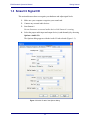


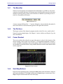
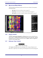
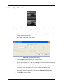

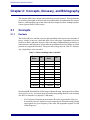


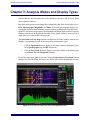


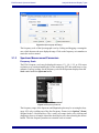
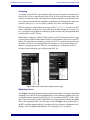
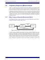

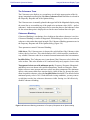

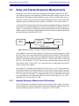
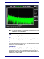
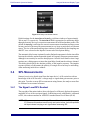


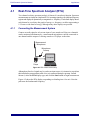
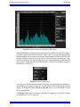
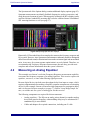
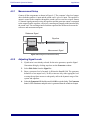

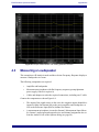
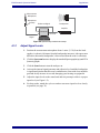
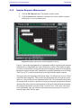


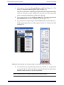
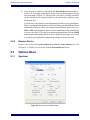
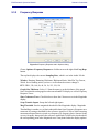


![[ siamo pronti al soccorso più pronto che immagini ] We are safety](http://vs1.manualzilla.com/store/data/006136853_1-948a1218599d528bc9a8bfb3fdadaf2c-150x150.png)