1
EE13
Updating Selected Laboratories
for Engineering Experimentation Course at Worcester Polytechnic Institute
A Major Qualifying Project Report
Submitted to the Faculty
of the
WORCESTER POLYTECHNIC INSTITUTE
in partial fulfillment of the requirements for the
Degree of Bachelor of Science
By
_______________________
Mengjie Liu
Date: April 25, 2012
_______________________________
Cosme Furlong, Advisor
Abstract
This project aimed at updating two existing laboratories in Engineering Experiment
course at Worcester Polytechnic Institute: Strain and Pressure Measurement Laboratory and
Vibration Measurement Laboratory. Without major alternation to the experiment designs, the
author examined laboratory equipment, software and instruction materials for both laboratories.
Two alternative signal conditioners are recommended as replacements to the current
system; software is updated to improve usability; and comprehensive laboratory instructions are
developed based on existing materials. The updated materials are suitable for future use at WPI
and other universities.
Acknowledgements
I am grateful for all the help received during the process of this project. I thank my
advisor Professor Cosme Furlong for making this project possible, and for all the valuable
guidance and advices. I appreciate WPI Mechanical Engineering department for providing the
experiment equipment, especially Lab Manager Peter Hefti for offering help and support in the
lab, and past Teaching Assistant for Engineering Experimentation course Ivo Dobrev for
providing helpful information.
This project builds upon existing laboratories developed faculty at WPI Mechanical
Engineering Department. I also want to acknowledge the wonderful work they have done with
this course.
2
Table of Contents
Abstract ........................................................................................................................................... 1
Acknowledgements ......................................................................................................................... 2
1.
Introduction ............................................................................................................................. 1
2.
Background ............................................................................................................................. 3
2.1
Contents and Implementation of the Course ................................................................ 3
2.2
Comparable Curriculums in Other Mechanical Engineering Programs ...................... 3
2.3
Current Design and Implementation of the Laboratories ............................................. 4
2.2.2
3.
Methodology ......................................................................................................................... 10
3.1
Selection of Alternative Signal Conditioners ................................................................. 10
3.1.1
Selection of Potential Alternative Signal Conditioners for In-Lab Testing............ 10
3.1.2
In-Lab Output Testing............................................................................................. 11
3.1.3
Comparison of Set-up Procedure ............................................................................ 13
3.1.4
Test Run of the Laboratories with Selected Signal Conditioners ........................... 14
3.2
4.
Opportunities for Improvements and Expansions..................................................... 5
Updating Software and Laboratory Instruction Materials.............................................. 14
Results ................................................................................................................................... 15
4.1
In-Lab Evaluation of Alternative Signal Conditioners ................................................. 15
4.1.1
Basic Information.................................................................................................... 15
4.1.2
Output Testing ........................................................................................................ 17
4.1.3
Set-up Procedure ..................................................................................................... 19
4.1.4
Selection of Alternative Signal Conditioner ........................................................... 24
4.1.5
Test Run of Selected Laboratories with Selected Signal Conditioners .................. 24
4.2
Updated Software and Instruction Materials ................................................................. 24
4.2.1
Updated Software.................................................................................................... 24
3
5.
4.2.2
Updated Instruction Materials for Strain and Pressure Measurement Laboratory 25
4.2.3
Updated Instruction Materials for Vibration Measurement Laboratory ................ 25
Conclusions and Future Work .............................................................................................. 27
Works Cited ...................................................................................Error! Bookmark not defined.
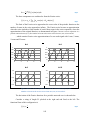
Appendix 1: Sample Laboratory Report for Strain and Pressure Measurement Laboratory ........ 30
Appendix 2: Sample Laboratory Report for Strain and Pressure Measurement Laboratory ....... 41
Appendix 3: Instructions for Strain and Pressure Measurement Laboratory ................................ 59
Appendix 4: Instructions for Vibration Measurement Laboratory ............................................... 90
4
Table of Tables
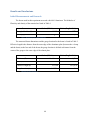
Table 1 Parameters for Testing ..................................................................................................... 12
Table 2 Comparison of Signal Conditioners’ Basic Parameters ................................................... 16
Table 3 Shunt Resistor Testing Result for Signal Conditioners ................................................... 17
Table 4 Accuracy Test Result ....................................................................................................... 18
Table 5 Output Noise of Signal Conditioners ............................................................................... 18
Table 6 Comparison Metrics for the Signal Conditioners ............................................................ 19
Table 7 Switch settings for Tacuna for 220 Gain ......................................................................... 20
5
Table of Figures
Figure 1 System Schematic of Strain Measurement Set-up.......................................................... 10
Figure 2 DATAQ’s Signal Response to Shunt Resistor ............................................................... 18
Figure 3 Connections for Tacuna Systems Strain Gauge or Load Cell Amplifier/Conditioner
Interface Manual ........................................................................................................................... 19
Figure 4 Location of Gain select switch and offset potentiometer ............................................... 20
Figure 5 Connections for Honeywell UV-10 In-line Amplifier ................................................... 21
Figure 6 Connections for Omega DMD 465-WB ......................................................................... 22
6
1.
Introduction
ABET accreditation criteria requires undergraduate engineering programs to prepare
students with “an ability to design and conduct experiments, as well as to analyze and interpret
data”, and mechanical engineering curriculums to “require students to apply principles of
engineering, basic science and mathematics”, and “prepare students to work professionally in
both thermal and mechanical systems.” (ABET, 2012)
The Engineering Experimentation course at WPI is designed to “develop analytical and
experimental skills in modern engineering measurement methods, based on electronic
instrumentation and computer-based data acquisition systems” (WPI, 2012). The lectures address
topics in engineering analysis and design, and the principles of instrumentation. (WPI, 2012)
It is the common understanding that the current laboratories in the WPI Engineering
Experimentation course can benefit from further efforts of improvement. Two existing laboratory
experiments from the Engineering Experimentation curriculum are selected as targets of
improvement: the Pressure Measurement Laboratory and the Vibration Measurement Laboratory.
The Pressure Measurement Laboratory performs characterization of internal pressure in
soda cans by measurements of strain, and conducts uncertainty analysis of characterized internal
pressures. (Furlong, Lab: Strain and Pressure Measurement, 2013) The Vibration Measurement
Laboratory determines the vibration amplitude, velocity, and acceleration, determines natural
frequencies and damping characteristics, and estimates elastic modulus of the cantilever used.
The results are then compared with analytical and/or computational models, uncertainty analysis
is then performed. (Furlong, Lab: Vibration Measurement, 2013)
This project aims at improving the laboratories by updating the instructive materials and
experiment equipment. The experiment designs will remain unaltered, suggestions for expanding
the experiment designs are included for future reference. The aspects for improvement include:
Educational Value.
Provided instructive materials and equipment should assist the students to meet
the defined objectives of the laboratories, and gain critical understanding of the physical
phenomenon, experimentation concepts, instrumentation principles, and data analysis
1
techniques involved. The equipment should enable acceptable level of accuracy and
resolution.
Student Experience.
The instructive materials should prepare the students with relevant theoretical
background, give clear and organized instructions that are easy to follow, and provide
challenging questions and assignments. The equipment should be safe and easy to operate,
and it should enable hands-on experience to deepen students’ understanding of the
equipment’s operating principle. Basic troubleshooting instructions should be provided
to the students and instructors to assist problem solving.
Cost-Effectiveness
Equipment for the laboratories should be low cost and adaptable for other
purposes of use. The perishable supplies should provide sufficient learning experience
before being consumed.
This project closely evaluates the existing laboratories and practices at other institutes
regarding similar experiments, and identifies goals for improvement according to the evaluation.
The identified issues are then addressed, and the updated laboratory is reevaluated after solutions
are implemented. Afterwards, opportunities to expand the experiment designs are explored.
In this project, an alternative strain gauge amplifier is selected from in-lab preliminary
evaluation of four suitable products; updated instructive material and sample reports are
generated for future Engineering Experimentation sections at WPI; and a literature research is
conducted to identify opportunities of expansion upon the current experimentation designs.
This report documented the process of this project in detail. The background section,
includes descriptions of the experiment procedures, sample results, an overview of practices at
other institutes, and identified areas for improvement of the existing laboratories.
The
methodology section includes the method used to evaluate and compare the existing and
potential alternative strain gauge amplifiers, and the method used to evaluate the measurements
acquired from the selected alternative amplifier.
2
2.
Background
2.1
Contents and Implementation of the Course
The Engineering Experimentation course at WPI is a junior-level compulsory course for
the Mechanical Engineering program; the coursework is equivalent to 3 credits. Before taking
this course, students are recommended to finish the compulsory fundamental courses in ordinary
differential equations, thermal-fluid, mechanics, and material science.
The topics addressed in this course include: review of engineering fundamentals,
discussions of standards, measurement and sensing devices, experiment planning, data
acquisition, analysis of experimental data, and report writing, etc. The laboratory periods exposes
students to modern devices in experiments, which involves both mechanical and thermal systems
and instrumentation in mechanical engineering. The students are trained to use modern
measurement and data acquisition systems, to process data with computer software, and to
produce formal laboratory reports.
The course provides two one-hour lectures and two three-hour lab periods every week
throughout a WPI’s seven-week term. Five laboratories with various focus and difficulties are
included.
2.2
Comparable Curriculums in Other Mechanical Engineering Programs
As essential parts of Mechanical Engineering skillset, topics from engineering
experimentation methods and techniques are often covered in undergraduate required
curriculums, and many programs provide electives for students to utilize and to further
strengthen skills in this area. The lectures are often accompanied by weekly laboratories that
focus on important topics mentioned in lectures; term projects are sometimes required.
The author conducted a primary curriculum study performed on around 70 top-ranked
undergraduate Mechanical Engineering programs according to the information from university
catalogs and course content websites. This study helped to identify the topics frequently taught at
state-of-art education institutes. Application of probability and statistics, uncertainty analysis,
calibration, resolution, precision, basic measurement techniques, basic signal conditioning, and
technical communication are addressed by almost all programs investigated. However, these
topics are often scattered in several courses taught at different times.
3
Familiarity of computerized data acquisition system is cultivated in required courses in
the majority of programs investigated, and a significant amount of programs teaches the use of
traditional tools such as oscilloscope and function generator. Other frequently taught topics
include frequency response and Fourier transformation, experiments in fluid mechanics, and
material testing. In the programs where control theory is a required content, experimentation
laboratories often include a section in control as well.
However, there are at least seven programs among the investigated ones that do not
dedicate coursework to address experimentation methodology and techniques, or introduces
these contents in a half course laboratory focused in other subjects such as material property.
2.3
Current Design and Implementation of the Laboratories
The laboratories cover measurements of resistance, calibration of pressure sensors,
measurement of pressure with strain gauges, measurement of vibration with strain gauges, and
calibration of thermistors.
Data acquisition system is used in all the laboratories, where LabVIEW programs are
used to facilitate data acquisition and processing. Mathematical programs are used in data
analysis. A formal lab report is required for each laboratory.
The lengths of the laboratories vary from one three-hour lab period to four periods.
During the lab periods, the instructor explains the procedures and important issues, and helps
students with trouble shooting when they are performing the experiment.
The Strain and Pressure Measurement laboratory teaches pressure characterization of
thin-wall vessel, uncertainty analysis of the result is also required. Combined with the signal
conditioning system and analog/digital converter, strain gauges are utilized to detect the change
in surface strain when the soda cans are opened; the strains are transferred to sensitive readings
in voltage with a Wheatstone bridge, and then used to determine the pressure difference after it is
amplified with a pre-amplifier.
The Vibration Measurement Laboratory focuses on dynamic measurement of a freevibrating cantilever beam, the measured characteristics are then used to estimate the elastic
modulus of the beam; uncertainty analysis of the results is also required. Same set-up is used to
4
acquire data in strains as the Strain and Pressure Measurement Laboratory, including strain
gauges, a Wheatstone bridge, a signal conditioning system, and an analog/digital converter.
2.2.2
Opportunities for Improvements and Expansions
Laboratories that measures pressure and vibration with strain gauges are frequently
taught at colleges. A review of the similar laboratories developed by other organizations provides
insights for the opportunities for improvements and expansions of the current laboratories at WPI.
More areas for improvements are suggested from a close examination of the current laboratories.
2.2.2.1 Design of Strain and Pressure Measurement Laboratory
The current set-up provides reliable measurements with an impressive micro-strain level
resolution, which is enabled by the 16-bit A/D converter and the signal conditioner. However,
the current laboratory does not fully utilize the set-up to reinforce the students’ appreciation of
resolution and the benefits of signal conditioning in the laboratories. The students can benefit
from additional activities to measure the resolution and noise under different gain settings and
the A/D converter’s range settings.
The current laboratory focuses on demonstrating pressure measurement with strain
gauges. The strain gauges are installed on soda cans, and once the cans are opened, the gauges
cannot be reused. Adding a few more activities to the existing laboratory could help utilize the
perishable materials more sufficiently. For example, an experiment conducted at Purdue
University College of Technology at New Albany proved that turning the can end to end twice
after shaking the can for 5 seconds will drastically reduce the measured strain in soda can
experiment. (Dues, 2006) The results from this experiment showed that the strain measured after
turning the can end to end twice is 90% lower than the strain measured directly after shaking the
can for 5 seconds. (Dues, 2006)
It is not uncommon for undergraduate laboratories to take advantage of a “class data
sheet” to increase the size of data set, which often provides more opportunity to practice the
statistical data analysis, and to draw significant conclusions to the phenomenon investigated. In
the case of this specific laboratory, multiple sources of errors exist in the strain gauge installation
process, such as alignment, surface condition of the adherence, wiring, etc. The property
measured, internal pressure of a soda can, can be easily affected by the person conducting the
measurement, as the solubility of carbon dioxide in the beverage can be affected as local
5
temperature and pressure vary, which unsettles the equilibrium of fluids and carbon dioxide in
the can. For these stated sources or variability, the students can gain more insights of the
experiment from a relatively large amount of measurements. Therefore, use of a “class data sheet”
to gather experiment results can be beneficial. In addition, due to the different carbonation
processes in the beverage products, beverage cans of one product should be provided to the
whole class to acquire more meaningful data.
Strain gauge rosettes, or a set of single strain gauges arranged in different directions, can
characterize the principle stresses of a surface. Strain measurements in multiple axes can provide
valuable learning experience to students. A student laboratory used at Middle East University
uses a three element rectangular rosette with an unknown angle α to the axis of a thin-wall vessel
to measure the internal pressure of the vessel. (Middle East Technical University) The material’s
Poison’s ratio, the unknown angle α, the direction and magnitude of principle stresses, principle
strains are also determined as a part of the laboratory. More in-depth engineering calculations are
utilized in the mentioned laboratory, and the introduction of strain rosettes adds breadth to the
basic design of laboratory.
2.2.2.2 Design of Vibration Measurement Laboratory
Since the vibration measurement laboratory shares the same set up with the strain and
pressure measurement laboratory, investigation of the resolution and noise under different gains
and the A/D converter’s range settings can be conducted in this laboratory as well.
Calibration of the strain measurement system can be taught with the current setup of this
laboratory. A laboratory taught at Northern Illinois University requires students to determine the
strain gauges’ gage factors by applying known weights, which is directly leads to known strains.
(Mostic, 1990) A laboratory taught at University of Massachusetts Lowell teaches students to
determine the systems’ sensitivity by applying known deflection, so that the output voltage can
be associated with measured strain. (Mostic, 1990) The laboratory developed by Vernier
Software and Technology challenges the students to use the set-up as a penny-counter, which
will accurately count the number of pennies placed on the tip of the cantilever. (Mostic, 1990)
This laboratory teaches students to determine elastic modulus of the material by deriving
it through measured frequency, yet the determination of “effective length” for vibration of the
beam, which is a parameter in the calculation, is somewhat ambiguous in this laboratory. The
6
error in finding the “effective length” adds uncertainty to the elastic modulus estimation. The
boundary condition created by the fixture made of a c-clamp and the lab bench makes the set-up
slightly deviates from the simple cantilever model. The issue can be alleviated by simply adding
a piece of aluminum plate between the clamp and the beam. A special fixture tool with a
rectangle shape that rigidly clamps the beam can provide the ideal boundary condition. On the
other hand, a conventional method of determining elastic modulus can be used in conjunction to
the existing method for comparison: apply a series of known load to the tip of the beam while
measuring strain, so the stress-strain plot can be created for extracting the elastic modulus.
The current laboratory uses a quarter-bridge Wheatstone set-up. The laboratories can be
extended by introducing half-bridge and full bridge set-up for uniaxial bending strain
measurement. In addition to providing temperature compensation and higher sensitivity, the
different set-ups enable compensation for the effect of transverse strain, and/or for the effect of
lead wire resistance. (Acromag)
Multi-axial strain measurement with a cantilever opens up opportunities for enriching the
current vibration laboratory and developing new laboratories. Besides principle stress and strain
under bending, which can be directly derived from strained measured in different directions,
Poisson’s ratio and stress concentration factor are among the characteristics the set-up can
measure.
Poisson’s ratio of the material can be measured with two strain gauges mounted along
longitudinal and lateral axis at corresponding locations on opposite sides of the beam. In a
laboratory used at Arizona State University, a range of known stresses is applied to acquire the
corresponding longitudinal and lateral strain when the beam reaches stable state. The dataset is
examined for outliers and then used to calculate an average Poisson’s ratio. (Poisson's Ratio,
2003)
Stress concentration factor of a specific geometric discontinuity, such as a hole on a
cantilever, can be measured with a group of very small strain gauges with fine grids. The
characterization can be performed when the beam is loaded with point bending and/or tension
with different methods. The laboratory taught at New Mexico Tech fitted the measured data into
a stress distribution function to find the constants, which contribute to the calculation of the
concentration factor. (Ruff) Other data analysis methods for laboratories range from deliberate
7
Finite Element simulation (Kargar, S; Bardot, D.M. ., 2010) to simplified method of drawing a
smooth curve to connect the data points on a plot with distance from the hole against the local
strain (Stress and Strain Concentration, 2003).
When a set of strain gauges are installed at different positions on the longitudinal axis of
a cantilever beam, and a known bending load applied at the free end of the beam, a series of
beam characteristics can be determined, and the system can be calibrated to measure unknown
loads. A stress analysis laboratory taught at Middle East Technical University with such design
determines the beam’s flexural rigidity, height, location of the beam and location of the applied
load, and enables the system to measure loads. (Middle East Technical University)
The current laboratory derives natural frequency of the beam by analyzing the vibration
data during free vibration. Another alternative method to determine natural frequency is to find
the resonance profile of the beam, or the amplitude response at each frequency under forced
vibration of constant amplitude input. This method is taught in certain curriculums, for example,
in the Aerospace laboratory course at University of Toronto. (Emami)
2.2.2.3 Equipment
While some improvements can be implemented without major change in the equipment
list, the existing resources do not support measurement of strain in multiple axes. The employed
signal conditioning unit, Vishay 2310 Signal Conditioning Amplifier System, is single-channeled
and relatively costly to acquire. An economical yet effective alternative signal conditioner should
be acquired to enable this upgrade, which will be discussed in section 3.1 and section 4.1 of this
report.
2.2.2.4 Laboratory Instructive Materials
The instructive materials should guide the students to prepare for the laboratory, conduct
the experiment and complete the lab report. Background knowledge of the key elements should
be provided to ensure sufficient appreciation of the topics; the experiment steps should be
described in details; and the discussion questions should help reinforce the knowledge and skills
acquired.
To help students further appreciate the Wheatstone bridge set-up with strain gauges, the
lab assignment should include calculations of current draw and power consumption of the circuit.
8
2.2.2.5 Software
The course requires no previous experience of programming in LabVIEW, therefore, the
instructive materials need to guide the students to construct simple functional programs to
facilitate the experiment. More advanced LabVIEW programs can be provided to the students to
use in the laboratories. Some of the suitable features to add to the basic programs are: filters,
data processing, and data reporting.
9
3.
Methodology
3.1
Selection of Alternative Signal Conditioners
3.1.1
Selection of Potential Alternative Signal Conditioners for In-Lab Testing
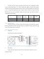
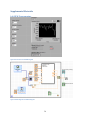
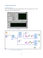
The two target laboratories, strain and pressure measurement laboratory, and vibration
measurement laboratory, use the same set up for strain measurement. The hardware set-up
includes a signal conditioner unit that supplies excitation voltage and amplifies output signal
from the Wheatstone bridge. The amplified signal is converted to digital signal by the A/D
converter, and then processed by software installed on a computer. Currently, NI6229, a 16 bit
DAQ instrument is used for the conversion, and LabVIEW program is used for data processing.
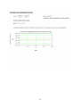
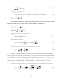
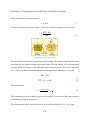
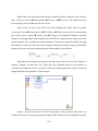
Figure 1 shows the system schematic of the strain measurement set-up.
Figure 1 System Schematic of Strain Measurement Set-up
The resolution of the experiments is determined by the signal conditioner gain setting,
A/D converter’s resolution, and its range. The range can be configured LabVIEW DAQ assistant
module. Since the resolution of an A/D converter of N bit is given by expression:
where N, the effective bit is 1.5 bit less than total bit.
10
In the case of the current set-up, the range can be set to 5V. Thus, the resolution is
0.22mV. Amplifier gain determines the transfer function between signal voltage and represented
strain. When gain is 200, the resolution represents 0.23 microstrain.
In order to enable successful implementation of the laboratories, suitable signal
conditioners should satisfy a series of requirements. Both laboratories uses strain gauges with
120Ω resistance, the signal conditioner should be able to provide quiet, accurate and stable
readings with selected strain gauges. The laboratories currently use a gain setting close to 200;
the signal conditioner should be able to offer a comparable gain. The vibration measurement
laboratory requires the signal conditioner to have a frequency response of over 1kHz. Gain
indication and bridge balancing are preferred, optional internal Wheatstone bride completion
circuit is another preferred feature. The cost for each unit of signal conditioner should be
relatively low, so that experiments involving multiple channels of strain measurement could be
developed in the future.
The currently deployed signal conditioner is Vishay 2310 Signal Conditioning Amplifier
System (Vishay 2310). Extensive search of available commercial products was conducted to
select the potential alternative systems that satisfy most criteria listed above.
3.1.2
In-Lab Output Testing
In-lab testing of the signal conditioners’ output is conducted. A quarter bridge completion
board is used for testing of all signal conditioners except Vishay 2310, which contains an internal
quarter bridge completion circuit.
The variable strain gauge is installed on an aluminum
cantilever beam with one foot of gauge 26 wires. For Omega, the gain was adjusted so that 1V
signal output corresponds to 800 microstrain. Table 1 shows the excitation and gain selected for
each signal conditioner for this testing. The signal conditioners require time to “warm up”, so
that optimum performance can be achieved. Table 1 shows the warm-up time used for each
signal conditioner during testing.
11
Vishay
Omega
Honeywell
DATAQ
2310
DMD-465WB
UV-10
DI5B38-04
Excitation
10V
10V
5V
10V
5V
Gain
191
239*
200
333.3
220
Warm-up
Time
0
45 min
10 min
10 min
5 min
Tacuna
Table 1 Parameters for Testing
Strain load can be simulated when a shunt resistor is connected to the Wheatstone bridge
in parallel to the active gauge. For the first output testing, three different shunt resistors are used
to simulate three different strains for each signal conditioner. For each shunt resistor, five
readings are taken with each signal conditioner. The three shunt resistors used in this testing
have the resistance of 12.88kΩ, 35.92kΩ, and 45.05kΩ, simulating strains of 4406 micro strain,
1751 micro strain, and 1268 micro strain respectively.
The shunt resistor is connected to the circuit before the recording starts. It is disconnected
from the circuit approximately five seconds after the recording starts. The recording continues
for 10 to 15 seconds until the readings stabilize for at least five seconds. A voltage reading is
acquired by calculating the absolute difference between the average voltage before disconnecting
the shunt resistor, and the average voltage after the signal stabilizes. The strain reading is given
by expression:
where
is the voltage reading, Gain is the amplifier gain,
is the excitation voltage,
and F is the excitation voltage.
The strain readings are evaluated for noise, accuracy and precision. The results of these
three parameters are compared for the four tested systems to eliminate systems with undesirable
performance.
12
The Error is the percentage difference between measured strain and simulated strain. The
Maximum Error is the largest observed error in the five samples taken. The Average Error is
given by:
̅
where
√
is the Error of each reading.
For each reading, the standard deviation of the signals after applying simulated load is
calculated; this is equivalent to RMS noise. Peak-to-peak noise amplitude is within 8 times RMS
value 98% of the time.
Note that the sources of measured output noise not only include the components in the
signal conditioner, but also include other hardware in the set-up. The set-up is designed to
simulate real conditions in the laboratories.
A second output testing is conducted with actual strain. With the clamped cantilever, a
known weight is attached to the free end of the beam, simulating strains between 200 micro
strain and 300 micro strain. Accuracy of 3 signal conditioners is tested by this method.
The test results for all four systems are reviewed and compared to eliminate systems with
less desirable performances.
3.1.3
Comparison of Set-up Procedure
The laboratories require systems that are easy and safe for students to connect and
balance. Gain setting and gain indication mechanisms are necessary. Among the signal
conditioners with acceptable performance (determined by in-lab output testing), the connection
layout, balancing procedure and gain setting procedure are compared to eliminate the ones
unsuitable for use in these laboratories.
Thus, the remaining systems should have both acceptable performance and suitable setup procedures to be used in selected laboratories.
13
3.1.4
Test Run of the Laboratories with Selected Signal Conditioners
Test run of the laboratories are performed with selected signal conditioners for further
validation. Sample laboratory reports are generated for reference.
3.2
Updating Software and Laboratory Instruction Materials
The current VIs is examined. Improvements are made to the program for usability,
without any major alternation of the program design. Detailed step-by-step tutorial for
constructing these VIs are written.
In the updated instructions, the key background topics are identified for each laboratory,
brief overview of the topics and derivations of key equations are provided. Optional activities are
developed for each laboratory based on the selected improvement opportunities for laboratory
designs, which are identified in the Background section. The optional activities are described in
attached documents to the instructions. The set-up and use procedures for the selected alternative
signal conditioner are included in the instructions. The detailed descriptions for the experiment
procedures are written based on the current instructions. Current materials include precise slides
and the instructor needs to explain the steps in person.
14
4.
Results
This project recommended two alternative signal conditioners for use in Strain and
Pressure Measurement Laboratory and Vibration Measurement Laboratory, and updated the
LabVIEW programs and instruction materials for both laboratories.
4.1
In-Lab Evaluation of Alternative Signal Conditioners
Extensive search for available commercial products, in-lab output testing for selected
potential products, and comparison of set-up procedures are conducted to generate
recommendations for alternative signal conditioners. Test runs of specified labs are conducted to
verify the conclusions.
4.1.1
Basic Information
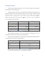
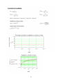
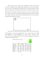
The basic parameters of Vishay 2310 are compared with potential alternative signal
conditioners in Table 2. The selected products include Omega DMD-465WB Bridge Sensor AC
Powered Signal Conditioner (Omega DMD-465WB), Honeywell UV-10 In-line Amplifier
(Honeywell UV-10), Tacuna Systems Strain Gauge or Load Cell Amplifier/Conditioner Interface
Manual (Tacuna), and DATAQ Instruments DI5B38-04 Strain Gage Input Modules (DATAQ
DI5B38-04). All five systems are single-channeled.
As shown in Table 2, all four alternative systems satisfy the basic requirements regarding
gain and frequency response. Honeywell and Tacuna meet the preferred requirements of
enabling bridge balance and gain indication.
15
Vishay
Omega
Honeywell
DATAQ
2310
DMD-465WB
UV-10
DI5B38-041
115VAC
115VAC
18 - 32 VDC
5VDC
6-16VDC
Excitation
0.5-15 VDC,
4 to 15VDC
3, 5 and 10 V,
Voltage
12 settings
Manual adjust
Manual adjust
10VDC
5VDC
Max 100 mA
Max 120mA
Max 70mA
70-170mA
Max 100 mA
Automatic
N/A
Manual
N/A
Manual
1-11000
40–250,
continuous
manual adjust
333.3
variable
potentiometer
110-11000, seven
switch settings;
Precision
programmable gain
Direct reading
No indication
Supply
Voltage
Current
Draw
Bridge
Balance
Gain
Gain
Indication
Output
Noise
5
Frequency
0.2
RMS
(when Gain=100)
switch settings
Shown by switches
on circuit board
55
RMS
No indication
2mV RMS
60kHz
2kHz
5kHz
10kHz
8.75”H 1.706”W
3.75”L 2.0”W
3.75”L 2.5”W
2.5” L 2.5”W
Response
Size
RMS
37.5-1000, 12
Cost
15.9” D
2.87”W
2.1”H
1.0”H
$2,200
$363
$350
$225
Table 2 Comparison of Signal Conditioners’ Basic Parameters
(Vishay Precision Group)
(Omega)
(Honeywell)
(Dataq)
(Tacuna Systems)
16
Tacuna
Shown by switches
on circuit board
Data unavailable
Factory
Adjustable
3.3” L 1.3”W
1.0”H
$117
4.1.2
Output Testing
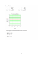
With the method described in section 3.1.2 of this report, the noise, accuracy, and
precision of measurements are evaluated. Table 3 shows the analysis results when the strains are
simulated with shunt resistors.
Vishay
Omega
Honeywell
DATAQ
2310
DMD-465WB
UV-10
DI5B38-04
0.24
2.46
2.14
4.99
0.18
0.24
3.94
4.09
11.44
0.31
1.93
19.71
16.8
39.95
1.44
1.93
31.49
32.7
91.54
2.48
Maximum Error
2.6%
9.3%
2.9%
12.5%
3.5%
Average Error
1.7%
7.1%
1.7%
9.7%
2.1%
0.65
0.36
0.54
4.55
3.90
0.65
0.57
1.04
10.43
6.77
Tacuna
Noise
Output Noise
(mV RMS)
Output Noise
(microstrain RMS)
Output Noise
(mV Peak-to-Peak)
Output Noise
(microstrain Peak-to-Peak )
Accuracy
Precision
Standard Deviation of Readings*
(mV)
Standard Deviation of Readings*
(microstrain)
Table 3 Shunt Resistor Testing Result for Signal Conditioners
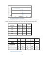
While the other tested signal conditioners responses to the change in simulated load
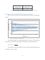
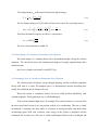
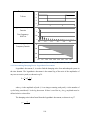
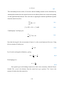
instantaneously, DATAQ occasionally shows response time as long as 3 to 5 seconds. Figure 2
shows the amplified signal output of DATAQ when the measurement starts at second 0, and
simulated load is removed at second 10.
17
Amplifiied Signal (V)
1
0.5
0
-0.5
0
5
10 Time (s) 15
20
25
Figure 2 DATAQ’s Signal Response to Shunt Resistor
With the method described in section 3.1.2 of this report, the noise, accuracy, and are
evaluated with actual strain of known values. Table 4 and Table 5 show the analysis results.
Applied Load
Omega
Honeywell
(micro strain)
DMD-465WB
UV-10
266.8
265.7
258.9
259.6
240.5
234.9
225.3
234
213.7
209.8
207.9
208.7
Error
2%
4%
2.5%
Tacuna
Table 4 Accuracy Test Result
Vishay
Omega
Honeywell
DATAQ
2310
DMD-465WB
UV-10
DI5B38-04
Output Noise
(mV-RMS)
0.30
0.55
0.72
1.25
0.14
Output Noise
(microstrain-RMS)
0.30
0.69
0.75
2.19
0.16
Output Noise
(mV-Peak to Peak)
2.38
4.43
5.77
10.05
1.10
Output Noise
(microstrain- Peak to Peak)
2.38
5.53
6.05
17.54
1.27
Table 5 Output Noise of Signal Conditioners
18
Tacuna
As shown in the test results, the current system, Vishay 2310, outperforms all other
system in all measured aspects. It is, however, significantly higher cost than all other systems
considered. The measured performance metrics for the four considered amplifier are ranked from
1 to 4, 1 being the best performance and 4 being the worst. As shown in Table 6, DATAQ
DI5B38 shows the lowest performance compared to other systems, and therefore should be
eliminated from the selection.
Omega
Honeywell
DATAQ
DMD-465WB
UV-10
DI5B38-04
2
3
1
3
1
2
4
4
4
Noise
Accuracy
Precision
Tacuna
1
2
3
Table 6 Comparison Metrics for the Signal Conditioners
4.1.3
Set-up Procedure
The set-up procedures for Tacuna, Honeywell and Omega are described and compared.
Discrete gain setting mechanism and gain indication are desirable features, and devices with
easier connecting procedures are preferred.
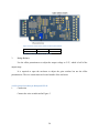
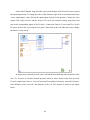
4.1.3.1 Set-up Procedure for Tacuna
1.
Connection
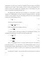
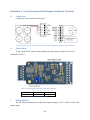
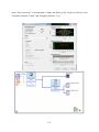
Connect the wires as indicated in Figure 3.
Figure 3 Connections for Tacuna Systems Strain Gauge or Load Cell Amplifier/Conditioner Interface Manual
2.
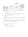
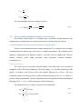
Gain Setting
To get a gain of 220, make sure the switches (location shown in Figure 4) are set as
indicated in Table 7.
19
Figure 4 Location of Gain select switch and offset potentiometer
G0
ON
G1
OFF
G2
OFF
Table 7 Switch settings for Tacuna for 220 Gain
3.
Bridge Balance
Use the offset potentiometer to adjust the output voltage to 2.5V, which is half of the
output range.
It is required to open the enclosure to adjust the gain switches but not the offset
potentiometer. The wire connections are located outside of the enclosure.
4.1.3.2 Set-up Procedure for Honeywell UV-10
1.
Connection
Connect the wires as indicated in Figure 5.
20
Figure 5 Connections for Honeywell UV-10 In-line Amplifier
2.
Gain setting
While excitation jumper is set to 5V, in order to get a gain of 200, make sure switch 3
and switch 6 are on and other switches are off.
3.
Calibration
With zero loads on the strain gauge, adjust the ZERO potentiometers until the reading
approaches 0.
It is required to open the enclosure to adjust both the ZERO potentiometers and the gain.
The wire connections are located inside the enclosure as well.
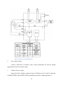
4.1.3.3 Set-up Procedure for Omega DMD-465 WB
1.
Connections
Connect the wires as indicated in Figure 6.
21
Figure 6 Connections for Omega DMD 465-WB
2.
Set excitation voltage
Connect a multi-meter to terminal 2 and 4; adjust potentiometer B+ until the reading
approaches the desired excitation voltage.
3.
Calibrate for zero voltage
Jumper pin 8 and 9 together, connect the inputs of DAQ box to pin 11 and 10. Adjust the
COARSE OFFSET and the FINE OFFSET potentiometers until the voltage approaches 0.
22
4.
Adjust gain
Connect the shunt resistor simulating strain desired for full scale. Adjust the COARSE
GAIN and FINE gain potentiometers for the desired full scale output.
All wire connections and potentiometers of this equipment are located on the surface of
the enclosure. No discrete gain setting is available, or any gain indications.
4.1.3.4 Comparison of Set-Up Procedures
Due to its lack of discrete gain setting mechanism and gain indication, and long set-up
procedure, Omega is less suitable for the target laboratories. Honeywell and Tacuna are
relatively easy to hook up and calibrate. For both systems, it is recommended that the
connections to be extended to avoid wear of the connection pieces and reduce issues caused by
bad connections in lab.
Comparing Honeywell UV-10 and Tacuna, Tacuna is more preferable. The students
won’t be required to open the enclosure of Tacuna if the gain setting is preset prior to the
laboratory, while the students need to open the enclosure of Honeywell UV-10 to adjust the
ZERO potentiometers, which might induce more complexity to managing the laboratories.
Tacuna also includes internal Wheatstone bridge completion circuit, in additional to the external
circuit set-up option tested in this project.
23
4.1.4
Selection of Alternative Signal Conditioner
Tacuna Systems Strain Gauge or Load Cell Amplifier/Conditioner Interface Manual
(Tacuna) provides reliable and quiet reading, and easy set-up experience. It is most viable
economical alternative to currently used signal conditioner.
Honeywell UV-10 In-line Amplifier provides satisfying performances as well, and a setup experience slightly more complex than Tacuna. It is more costly compared to Tacuna, but
also significantly more economical compared to the current system.
Out of the four signal conditioners considered, Tacuna is recommended as the top choice,
while Honeywell UV-10 is recommended as the second choice.
4.1.5
Test Run of Selected Laboratories with Selected Signal Conditioners
Test runs of both laboratories are performed with both Tacuna and Honeywell UV-10, no
problematic issues were encountered with the alternative equipment, and the experiments were
all successful.
Sample laboratory reports of both laboratories performed with Tacuna are included in
Appendix 1 and Appendix 2.
4.2
Updated Software and Instruction Materials
Updated software and instruction materials are produced for both laboratories. This
section describes the improvements on the software features and the contents of the instruction
material.
4.2.1
Updated Software
Updated VI for both labs added elements to the file output function. Using Write to
Measurement File instead of Write to Spreadsheet adds a column for elapsed time, which makes
the data more complete. The data is saved under the same directory as the program, with
standardized file names and “.csv” extension.
Updated software for Strain and Pressure Measurement Laboratory incorporated some
improvements of the existing VI, which include:
The LabVIEW Formula function is used to calculate strain, pressure and stresses, instead
of Formula Node. The Formula function can process dynamic data input, while the Formula
24
Node requires dynamic data to be converted to numerical data. This enables the program to
process and record all acquired data points.
The updated VI allows the user to input excitation voltage, gain, and gage factor; thus the
program can be used with different hardware conditions without major alternation.
Updated software for Vibration Measurement Laboratory enables saving time domain
data without alternating the program.
Step-by-step tutorials for constructing the programs are included in the updated
laboratory instructions, which are contained in Appendix 3 and Appendix 4.
4.2.2
Updated Instruction Materials for Strain and Pressure Measurement Laboratory
The background part of updated instruction material for Strain and Pressure Measurement
Laboratory contains brief overviews of following topics:
Piezoresistive pressure sensor
Stress and strain in a thin-wall cylinder
Strain gages
o
Operating principle and application of strain gages
o
Materials and selection of strain gauges
Wheatstone bridge
The instructions describe the experiment procedures in detail, propose data analysis tasks
and discussion questions, and include optional activities and relevant reference information.
Refer to Appendix 3 for the instructions document.
4.2.3
Updated Instruction Materials for Vibration Measurement Laboratory
The background part of updated instruction material for Vibration Measurement
Laboratory contains brief overviews of following topics:
Static analysis of simple cantilever beam
o
Stress, strain, and deflection associate with bending
o
Calculation of static characteristics
Dynamic characteristics of a cantilever beam under free vibration
o
Natural frequencies of a cantilever beam under free vibration
25
o
Mode shapes of a cantilever beam under free vibration
o
Damping factor of a cantilever beam under free vibration
Measurement methods of dynamic characteristics
o
Fourier transformation
o
Logarithmic decrement method to determine damping frequency
o
Determining acceleration, velocity and amplitude
o
Determining elastic modulus
Strain gages
o
Operating principle and application of strain gages
o
Materials and selection of strain gauges
Wheatstone bridge
The instructions describe the experiment procedures in detail, propose data analysis tasks
and discussion questions, and include optional activities and relevant reference information.
Refer to Appendix 4 for the instructions document.
26
5.
Conclusions and Future Work
This project examined two existing laboratories in WPI’s Engineering Experiment course
and made a series of recommendations and actions, in the hope of improving the educational
value, student experience and the cost-effectiveness of the laboratories.
The project recommended two alternative signal conditioners to use in the laboratories.
Both signal conditioners provide satisfactory performance and student experience, in addition to
being economical. Adopting either of the recommended models will help reduce expenses, and
enable dual or multiple axes measurements.
Software and laboratory instruction materials are updated. The software updates
improved user experience of the existing program. The instruction materials contain
comprehensive information to assist the students and instructors to prepare for and conduct the
experiments.
A review of similar laboratories developed by other institutes is included in the
background section of this report. Future effort of improving and expanding the laboratories can
be focused on introducing measurement of strain multiple axes for both labs, it will provide more
depth to the existing laboratories.
If the recommendations and updated materials are adopted, a brief survey can be
conducted to study the effects of the changes. Inputs from instructors and students are valuable
as references for future efforts to improve the laboratories.
27
Works Cited
Poisson's Ratio. (2003). Retrieved December 2012, from Fulton School of Engineering, Arizona State
University: http://enpub.fulton.asu.edu/imtl/HTML/Manuals/MC102_Poisson's_Ratio.html
Stress and Strain Concentration. (2003). Retrieved Febuary 2013, from Fulton School of Engineeing,
Arizona State University:
http://enpub.fulton.asu.edu/imtl/HTML/Manuals/MC104_Stress_Concentration.htm
ABET. (2012). Criteria for Accrediting Engineering Programs, 2012 - 2013 . Retrieved December 2012,
from ABET:
http://www.abet.org/uploadedFiles/Accreditation/Accreditation_Process/Accreditation_Docum
ents/Current/eac-criteria-2012-2013.pdf
Acromag. (n.d.). Introduction to Strain & Strain Measurement. Retrieved Febuary 2013, from Acromag:
http://www.weighing-systems.com/TechnologyCentre/Strain1.pdf
Dataq. (n.d.). Strain Gage Input Modules, Narrow and Wide Bandwidth. Retrieved 2012, from Dataq
Instrument: http://www.dataq.com/support/documentation/pdf/manual_pdfs/di5b38.pdf
Dues, J. F. (2006). Soda Can Myth Busting . The Technology Interface Journal.
Emami, F. (n.d.). Strain Gauge and Material Testing. Retrieved 2013, from Univerisity of Toronto:
http://www.aerospace.utoronto.ca/pdf_files/strain.pdf
Furlong, C. (2013). Lab: Strain and Pressure Measurement. Retrieved January 2013, from Cosme
Furlong's Engineering Experiementation Course:
http://users.wpi.edu/~cfurlong/me3901/lab03/Lab_3_Strain_D12.pdf
Furlong, C. (2013). Lab: Vibration Measurement. Retrieved January 2013, from Cosme Furlong's
Engineering Experimentation Course:
http://users.wpi.edu/~cfurlong/me3901/lab04/NotesLab04_P01.pdf
Honeywell. (n.d.). Bridge Based Sensor In-Line Amplifier. Retrieved 2012, from Honeywell:
https://measurementsensors.honeywell.com/ProductDocuments/Instruments/Model_UV10_Datasheet.pdf
Kargar, S; Bardot, D.M. . (2010). Uncertainty Analysis, Verification and Validation of a Stress
Concentration in a Cantilever Beam. COMSOL Conference . Boston.
Middle East Technical University. (n.d.). Lab 5: Stress Analysis Using Strain Gauges. Retrieved January
2013, from Middle East Technical University:
http://www.me.metu.edu.tr/courses/me410/exp5/me410_exp5_experiment_2011.pdf
28
Mostic, K. (1990). Lab: Calibration of and Measurement with Strain Gages. Retrieved Dec 2012, from
Northen Illinois University: http://www.kostic.niu.edu/Strain_gages.html
Omega. (n.d.). User's Guide. Retrieved from Omega:
http://www.omega.com/manuals/manualpdf/M1429.pdf
Pryputniewicz, R. (1993). Notes: Engineering Experiementation. WPI.
Ruff, J. (n.d.). Lab 6: Stress Concentration. Retrieved 2012, from New Mexico Tech:
http://infohost.nmt.edu/~jruff/Lab6.pdf
Tacuna Systems. (n.d.). Embedded Strain Gauge and Load Cell Signal Conditioner/Ampli. Retrieved 2012,
from Tacuna Systems: http://tacunasystems.com/zc/documents/EmbSGB1_2.pdf
Vishay Precision Group. (n.d.). Signal Conditioning Amplifier. Retrieved 2012, from Vishay Precision
Group: http://www.vishaypg.com/docs/11255/syst2300.pdf
WPI. (2012). WPI Undergraduate Catalog. Retrieved Dec 2012, from Worcester Polytechnic Institute:
http://www.abet.org/uploadedFiles/Accreditation/Accreditation_Process/Accreditation_Docum
ents/Current/eac-criteria-2012-2013.pdf
29
Appendix 1: Sample Laboratory Report for Strain and Pressure
Measurement Laboratory
Abstract
In this experiment, characterization of internal pressure in a thin-walled tank (a soda can)
is achieved by measurements of mechanical strains. Uncertainty analysis of characterized
internal pressure is conducted with respect to parameters involved. The percentage contribution
of all uncertainties to the overall uncertainty in pressure characterizations are identified in order
of importance.
Description
Purpose of the Experiment
The purposes of this experiment include:
Perform characterization of internal pressure in a thin-walled tank by measurements of
mechanical strains;
Perform uncertainty analysis of characterized internal pressures with respect to
parameters involved;
Identify, in order of importance, percentage contribution of all uncertainties to the overall
uncertainty in pressure characterizations.
30
Experimental Procedures
In order to understand the errors in this experiment, the procedure is repeated on three
soda cans of the same product.
Preparation
Find the Poisson’s ratio and elastic modulus of the material used for the soda cans.
LabVIEW Program
The constructed LabVIEW program obtains amplified voltage output and transfers the
output to strain, with the unit of micro-strain. A formula block calculates pressure and stress
from measured strains. Measurement results are recorded. Assume 0.005 inch as can thickness.
Hardware Setup
A strain gauge is installed onto each of the three soda cans used in this experiment.
Measure the diameter of the soda can.
The strain gauge is installed on the soda can surface along the circumferential direction,
the height of the strain gauge location should be half of the can height.
The strain gauge is connected to the quarter bridge completion circuit. A Tacuna Systems
Strain Gauge or Load Cell Amplifier/Conditioner Interface Manual (Tacuna) is used to supply
excitation voltage and amplify the signal. Gain is set at 220, while the excitation is set at 5 VDC.
The settings are verified by checking the switches on the circuit board. The wire connections are
indicated in Figure 1.
Figure 7 Connections for Tacuna Systems Strain Gauge or Load Cell Amplifier/Conditioner Interface Manual
31
Bridge Balancing and Verification
Make sure then NI DAQ box is turned on before starting the VI. Adjust the measurement
time to 0.01 second on the LabVIEW program to view instant strain readings. Use the offset
potentiometer to adjust the output voltage to 2.5V, which is half of the output range.
Connect shunt resistors parallel to the active gauge, and observe appropriate change in
the strain reading.
Gently press on the tap of the can, and observe the strain readings change accordingly.
Take Measurements
Allow the amplifier to warm up for 5 minutes before taking measurements.
For each can, record strain readings for approximately 5 seconds before opening the can,
and stop the VI 10 about seconds after opening the can. Use 0.005 inch for thickness during
recording. After clearing out the beverage in the can and cleaning the can, measure the thickness
of the can wall with a caliper. Take the average value of three measurements. Adjust the data
according to the new thickness measurement.
32
Key Equations
The expression for internal pressure of a thin-wall vessel can be given by:
where E is Elastic Modulus of the material,
is the Poisson’s ratio of the material, t is the
wall thickness of the vessel, r is the radius of the vessel,
is the strain in hoop
(circumferential) direction.
The stress in circumferential direction and axial direction is given by:
where P is internal pressure of the vessel, r is the radius, and t is the wall thickness.
Equipment List
National Instruments USB-6229 DAQ
Tacuna Systems Strain Gauge or Load Cell Amplifier/Conditioner Interface Manual
Wheatstone Bridge Quarter Bridge Completion Circuit
Vishay Strain Gage
Shunt Resistors
Three Cans of Soda of The Same Type
33
Results and Conclusions
The results of the characterization are listed in Table 1. The parameters are calculated by
taking the differences of the average values prior to opening of the cans and the average values
after opening the cans.
Can 1
(Fanta 355ml)
Can 2
(Fanta 355ml)
Can 3
(Fanta 355ml)
Pressure
Hoop Strain
Hoop Stress
Axial Stress
(psi)
(micro-strain)
(psi)
(psi)
35.0
750
43.7
937
48.2
1034
Table 1 Characterization Result
From the data acquired with three Fanta 355ml cans, it can be concluded that the pressure
in measured cans is in the range of 30 to 50 psi at room temperature.
34
Uncertainty Analysis
The parameters in Table 2 are used to perform uncertainty analysis for characterized
internal pressure. The detailed process of the analysis is included in the appendix.
Parameter
Young's Modulus (psi)
Poisson's Ratio
Thickness (in)
Radius (in)
Strain (micro strain)
Value
Uncertainty
0.35
0.005
1.300
0.005
3%
Table 2 Initial Parameters for Uncertainty Analysis
The uncertainty for measured pressure is constant at 10.4% when strain is within the
specified range. The percentage contributions of each variable (when strain = 900 micro strain)
are listed in the table below.
Parameter
Thickness
Strain
Poisson's Ratio
Radius
Young's Modulus
Contribution to Uncertainty
91.63%
8.25%
0.084%
0.034%
0.009%
Table 3 Percentage contribution to uncertainty
35
Supplemental Materials
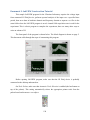
LabVIEW Programming
Figure 8 Front Panel of LabVIEW Program
Figure 9 Block Diagram of LabVIEW Program
36
Uncertainty Analysis
37
38
39
40
Appendix 2: Sample Laboratory Report for Strain and Pressure
Measurement Laboratory
Abstract
In this experiment, strain gauges are used to measure the dynamic characteristic and the
material properties of cantilevers. The vibration data is analyzed to determine the parameters; the
values derived from measurements are then compared with theoretical values and/or
computational models.
41
Description
Purpose of the Experiment
The purpose of the vibration measurement experiment is to use strain gauges to measure
the dynamic characteristic and the elastic material properties of cantilevers. Vibration data will
be analyzed to:
Determine the vibration amplitude, velocity, and acceleration in various units of measure;
Determine natural frequencies;
Measure and express damping characteristics as logarithmic decrement and percentage of
critical damping;
Compare measurements with analytical and/or computational models of a cantilever; and
Determine elastic modulus of a cantilever
42
Experimental Procedures
In order to understand the errors in this experiment, the procedure is repeated on two
similar cantilever beams.
Preparation
Find the elastic modulus and density of the material used for the cantilever beams.
LabVIEW Program
The constructed LabVIEW program obtains amplified voltage output and transfers the
output to strain, with the unit of micro-strain. A spectral analyzer performs Fourier
Transformation on measured strains. Measurement results in both time domain and frequency
domains are then recorded. A sampling rate of 5k S/s is selected, and 5 seconds of data is
recorded in each reading.
Hardware Setup
A strain gauge is installed onto each of the three soda cans used in this experiment.
Measure the diameter of the soda can.
The strain gauge is installed on the soda can surface along the circumferential direction,
the height of the strain gauge location should be half of the can height.
The strain gauge is connected to the quarter bridge completion circuit. A Tacuna Systems
Strain Gauge or Load Cell Amplifier/Conditioner Interface Manual (Tacuna) is used to supply
excitation voltage and amplify the signal. Gain is set at 220, while the excitation is set at 5 VDC.
The settings are verified by checking the switches on the circuit board. The wire connections are
indicated in Figure 1.
Figure 10 Connections for Tacuna Systems Strain Gauge or Load Cell Amplifier/Conditioner Interface Manual
43
Bridge Balancing and Verification
Make sure then NI DAQ box is turned on before starting the VI. Adjust the measurement
time to 0.01 second on the LabVIEW program to view instant strain readings. Use the offset
potentiometer to adjust the output voltage to 2.5V, which is half of the output range.
Connect shunt resistors parallel to the active gauge, and observe appropriate change in
the strain reading.
Gently press on the tap of the can, and observe the strain readings change accordingly.
Take Measurements
Allow the amplifier to warm up for 5 minutes before taking measurements.
For each beam, continuously pluck the end of the cantilever for 30 seconds and record the
vibration decay curves.
44
Key Equations
Strain in a Cantilever under Known Load
The strain in a cantilever beam under a known load applied at the free end is given by:
where is the strain, P is the applied load, L is the length of the beam, x is the distance
between the clamped end and the interested location of strain, E is the elastic modulus, b is the
width of the beam, and T is the thickness of the beam.
In this experiment, the applied load is the weight of a known mass. Therefore, we have
where M is the mass and g is gravity.
Fundamental Frequency
The equation below describes how to predict natural frequencies of cantilever beams.
√
√
where E is elastic modulus, L is effective length of beam,
thickness of the beam. The dimensionless wave number
cantilever beams are: β1L = 1.8751=
10.99557=
, β5L = 14.1372=
, β2L = 4.6941=
, β6L = 17.279=
is the density, T is the
= 2 /wavelength.
values for
, β3L = 7.8548=
, β4L =
.
In this experiment, the effective length of the beam is close to the distance between the
outer edge of the clamp and the free end of the beam.
Vibration Amplitude, Velocity, and Acceleration
The group of equations below shows the relationship how altitude and frequency
determine position, velocity and acceleration during vibration.
̇
̈
45
The altitude is equivalent to maximum deflection at vibration peaks. The amplitude can
be given by:
Therefore, the maximum velocity and maximum acceleration can be expressed as:
Damping Ratio
A common method for analyzing the damping of an underdamped oscillation is the
logarithmic decrement method, for which the following relationships apply.
(
)
√
√
where
is the amplitude of peak i (i is an integer counting each peak), n is the number of
cycles being considered, is the log decrement,
is the undamped natural frequency, and
is the damped natural frequency. Both frequencies are in radiance per second. Note, it is assumed
that object oscillates about zero. If there is an offset in y, the
amplitude must be defined
relative to that offset.
Elastic Modulus
From the expression for natural frequency, the expression for elastic modulus can be
derived as:
where
is
natural frequency,
values for cantilever beams are
,
is density, L is effective length, T is thickness, and
=1.8751,
.
46
=4.6941,
=7.8548,
,
Equipment List
National Instruments USB-6229 DAQ
Tacuna Systems Strain Gauge or Load Cell Amplifier/Conditioner Interface Manual
Wheatstone Bridge Quarter Bridge Completion Circuit
Vishay Strain Gage
Shunt Resistors
Three Cans of Soda of The Same Type
A Cantilever Beam
47
Results and Conclusions
Initial Measurements and Research
The beams used in this experiment are made with 6061 Aluminum. The Modulus of
Elasticity and density of the material are listed in Table 1.
Parameter
Value (SI Unit)
Value (English Unit)
68.9GPa
Young’s Modulus (E)
0.0975 lb/in³
Density (𝜌)
Table 1 Material Property of 6061 Aluminum
The measured beam dimensions and the gauge location for the beam is listed in Table 2.
Effective length is the distance from the outer edge of the aluminum plate (between the c-clamp
and the beam) to the free end of the beam; the gauge location is defined as distance from the
center of the gauge to the outer edge of the alumni plate.
Value (SI Unit)
Value (English Unit)
1/8 in
Thickness (T)
0.0255m
1 in
Effective Length (L)
0.270m
10 5/8 in
Gauge Location (x)
0.0255m
1 in
Width (b)
Table 8 Dimensions of Beam 1
48
Verification of Correct Installation
To verify the correct installation, a weight attached close to the free end on the beam. The
analytical strain at strain gauge location is derived and compared with measured values, as
shown in Table 3. The error is within 3% compared to the theoretical strain derived, therefore,
the installation is correct.
Theoretical Strain
Measured Strain
(micro strain)
(micro strain)
240.5
235
Error
2.5%
Table 3 Comparison of Theoretical Strain and Measured Strain
Determine Natural Frequencies
The fundamental frequency is determined by finding the frequency of the first “peak” in
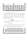
the power spectrum plot. Figure 1 shows results of Fourier Transformation from strain data
obtained from a vibrating beam.
Strain (Power Spectrum)
40
0
-40
-80
0
50
100
150
200
250
300
Hz
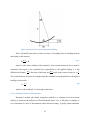
Figure 11 Power Spectrum of Strain
The fundamental frequencies of the two beams used in this experiment are determined
with this method. The measured value is then compared with theoretical undamped natural
frequency in the Table 4.
49
Theoretical Natural
Measured Natural
Frequency (Hz)
Frequency (Hz)
35.5
35.3
Table 4 Comparison of Measured Fundamental Frequency and Theoretical Fundamental Frequency
Determine the Vibration Amplitude, Velocity, and Acceleration
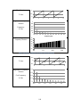
Figure 2 shows the plot for the strain measured from one of the beams during free
vibration.
Strain (micro strain)
200
100
0
-100
-200
2.9
3.4
3.9
Time (seconds)
Figure 12 Strain Measured from Vibrating Beam
The vibration amplitude, or maximum displacement at each peak, is derived from the
peak strain in the first vibration cycle and the beam dimensions with the relationship below.
The maximum velocity and acceleration is derived with the maximum displacement and
acceleration, as shown in Table 6.
50
Acceleration
Acceleration
Velocity
Amplitude
(m/s)
(m)
(g)
Peak
6.6
64.7
1.84
0.052
Peak-To-Peak
13.2
129.4
3.67
0.104
RMS
4.7
45.8
1.30
0.036
Table 5 Maximum Acceleration, Velocity and Displacement
Measure and Express Damping Characteristics
Using logarithmic decrement method, the damping ratio for the beam is determined from
measured data, as shown in Table 7.
Logarithmic Decrement
Damping Ratio
0.042
0.0067
Table 6 Damping Ratio
Predict Elastic Modulus.
The derived elastic modulus from the measurements and analytical prediction is listed
below. Predicted elastic modulus of the cantilever beam is 68GPa, the errors are close to
theoretical value.
Beam 1
Theoretical
Measured
Elastic Modulus (GPa)
Elastic Modulus (GPa)
68.9
68.2
Table 7 Comparison of Theoretical Elastic Modulus and Measured Elastic Modulus
51
Error
1%
Uncertainty Analysis
The uncertainty of natural frequency is 0.05 Hz, which is limited by the resolution of
spectral analyzer in LabVIEW program.
Uncertainty analyses with respect to the parameters are performed for damping ratio and
amplitude. Parameters used in the uncertainty analyses are shown in Table 9. Thickness, length
and gauge location are measured with a ruler, which has a least significant digit of
Therefore, the uncertainty for these three items is
inch, or
inch.
meter. An uncertainty
of 3% is assumed for measured strains.
Value
Uncertainty
Thickness (m)
Length
(m)
Gauge Location
Natural frequency
0.27
(m)
0.0254
(Hz)
35
Strain (micro strain)
0.05
3%
0 to
Table 8 Initial Values for Uncertainty Analysis
When logarithmic decrement is 0.043, the uncertainty for damping ratio is 9.9%.
Uncertainty in strain measurement is the only contributing factor.
The uncertainty for amplitude 25.2% when strain is within the range defined in Table 9.
The contributions of each factor are listed in Table 10.
Contribution
Thickness
98.5%
Strain
1.4%
Length
0.02%
Gauge location
0.02%
Table 9 Contributions of Parameters to Uncertainty in Amplitude
The steps of the uncertainty analysis are included in the Appendix.
52
Supplemental Materials
LabVIEW Program
Figure 3 shows the front panel of the LabVIEW program used in this experiment. Figure 4 shows
the block diagram of the LabVIEW program.
Figure 13 Front Panel of LabVIEW Program
Figure 14 Block Diagram of LabVIEW Program
53
Uncertainty Analysis
54
55
56
57
58
Appendix 3: Instructions for Strain and Pressure Measurement
Laboratory
Laboratory: Strain and Pressure Measurement
1.
OBJECTIVES
The objectives of this laboratory include:
Perform characterization of internal pressure in a thin-walled tank by measurements of
mechanical strains;
Perform uncertainty analysis of characterized internal pressures with respect to parameters
involved;
Identify, in order of importance, percentage contribution of all uncertainties to the overall
uncertainty in pressure characterizations;
59
2.
BACKGROUND
A thin walled cylinder has a wall thickness smaller than 1/10 of the cylinder’s radius. In this case, only
the membrane stresses are considered and the stresses are assumed to be constant throughout the wall
thickness.
The ASME boiler codes require continuous monitoring of pressure in thin walled pressure vessels. In
certain processes, use of mechanical pressure gauge or electrical pressure transducer to monitor the
pressure is unpractical, as the diaphragm can become encrusted with chemical products quickly.
Therefore, a new method is required.
2.1
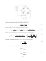
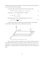
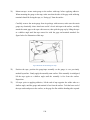
Piezoresistive Pressure Sensor
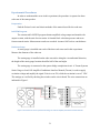
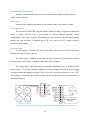
As shown in figure below, a pressure transducer consists of a diaphragm and four strain gages installed on
the metal film attached to the diaphragm. Note that strain gauges
strain gauges
the resistance of
and
and
and
are in the radial direction and
are in the direction transversal to the radius. Therefore, when pressure increases,
increases and
and
decreases. The four strain gages form a Wheatstone
bridge, as shown in figure below. The change in output voltage of a pressure transducer is directly
proportional to the change in pressure. The relationship between output voltage (
voltage (
) and the excitation
) is shown equation 1.
(
)
Figure 15a Cross Section of a Pressure Transducer
60
Eq.1
Figure 1b Top View of a Pressure Transducer
2.2
Figure 1c Circuit Diagram of a Wheat Stone Bridge
Stress and Strain in a Thin-Wall Cylinder
For vessels with a wall thickness of no more than one-tenth of its radius, the wall can be treated as a
surface. The law of LaPlace holds for fluid or gas filled hollow objects with radius r. For cylinders, the
internal pressure acts on them to develop a force along the axis of the cylinder.
Figure 16 Static equilibrium in cross-sections of a thin-walled cylinder
To determine the hoop stress
, equilibrium in the radial direction should be examined. As illustrated
in figure 2, the pressure acts to “pull the two halves apart”, while the hoop stress balances the effect. The
hoop stress yields,
Eq.1
Therefore,
Eq.2
61
Similarly, in the axial direction, the pressure acts to push the two halves apart, while axial stress balances
the effects, as shown in figure 3. The axial stress yields,
Eq.3
Eq.4
The Hooke’s Law states that stress in the can is proportional to the strain. The relationship in this case can
be expressed as:
Eq.5
where E is Elastic Modulus of the material, and
is Poisson’s ratio of the material.
With Eq.2, Eq.4, and Eq.5, the relationship between pressure and strains can be derived as:
Eq.6
2.3
Basics of Strain Gages
2.3.1
Operating Principle and Application of Strain Gages
Strain-gauge sensor is one of the most commonly used means of load, weight, and force detection. Strain
gauges are frequently used in mechanical engineering research and development to measure the stresses
generated by machinery, and in Aircraft component testing to structural measure stress of members,
linkages, and any other critical component of an airframe.
A strain gauge operates on the principle that the electrical resistance of a wire changes when the length of
the wire varies. It is used for measuring deformations in solid bodies. The strain experienced by the
sensor is directly proportional to the change in resistance of the gauge used, as shown in Eq 7.When
unstressed, usual strain gauge resistances range from 30 Ohms to 3 kOhms.
Eq.7
𝜌
An ideal strain gage is small in size and mass, low in cost, easily attached, and highly sensitive to strain
but insensitive to ambient or process temperature variations. The ideal strain gauge would undergo
change in resistance only because of the deformations of the surface to which the sensor is coupled.
However, in real applications, there are many factors which influence detected resistance such as
62
temperature, material properties, the adhesive that bonds the gage to the surface, and the stability of the
metal.
The strain sensitivity, which is also known as the gage factor (GF) of the sensor, is given by:
Eq.8
where R is the resistance of the gauge without deformation, dR is the change in resistance caused by
strain, and
is the strain to be measured. Therefore, the strain can be expressed as:
Eq.9
2.3.2
Materials and Selection of Strain Gauges
Typical materials for strain gages include: constantan (copper-nickel alloy), nichrome v (nickel-chrome
alloy), platinum alloys (usually tungsten), isoelastic (nickel-iron alloy), karma-type alloy wires (nickelchrome alloy), foils, and semiconductor materials. The most popular alloys for strain gages are coppernickel alloys and nickel-chromium alloys.
Temperature change can affect the internal structure of strain-sensing material, and also can amend
properties of the material of the surface the strain gage is attached to. When there is a temperature change
while a measurement is being made, the effects can cause large errors in data unless proper precautions
are taken.
Each material has unique reaction to temperature change, as illustrated in figure below. Variation in
expansion coefficients between the gage and base materials may cause dimensional changes in the sensor
element. Therefore, it is a good practice to select strain gauge made of same type of material as the base
structure.
63
Figure 17 Temperature Effects on Thermal Output of Strain Gauges
Strain gauge’s product name contains all critical information needed to select appropriate gauge. The
meanings of each part of the name are shown in Figure 18 below. While Figure 19 shows key information
of the type of strain gauge selected for this experiment.
Figure 18 Strain Gage Selection Steps
64
Figure 19 Crucial Information of Strain Gauge Selected
2.4
Basics of Wheatstone bridge
A Wheatstone bridge is an electrical circuit used to measure an unknown electrical resistance (from 1 Ω
to 1MΩ) by balancing two legs of a bridge circuit, one leg of which includes the unknown component. A
circuit diagram of Wheatstone bridge is shown in figure below, where the battery (symbol “E” serves as
an excitation source, and the output is measured by a potentiometer “G”).
A “balanced” bridge is one with potential difference between B and D is equal to zero. Balance is sensed
by closing switch S2 and measuring output current and voltage – to be near zero. Voltage drop across R2
is equal to voltage drop across R1, since voltage difference between B and D is equal to zero. Therefore,
Eq.10
65
Figure 6 circuit diagram of Wheatstone bridge
When the bridge is unbalanced, equivalent resistance of the circuit is,
Eq.10
When the circuit is viewed as a circuit divider, the output voltage is,
(
When the resistance of
)
(
Eq.11
)
changes by a small amount
, the new output voltage is,
Eq.12
(
If the bridge was originally balanced (
(
)(
)
)
, then we have,
Eq.13
(
Since change in resistance is really small
)
, the change in output voltage is,
or,
Eq.14
66
3.
PROCEDURES
In order to estimate the internal pressure of soda cans, the procedures of this experiment include research
for relevant data, hardware set-up, construction of LabVIEW program, signal conditioning, taking
measurements, and data analysis. The measurements should be repeated on 3 soda cans.
The information acquired from research and part of the measurement process should also be used to
produce uncertainty analysis and the contribution of each parameter to total uncertainty.
3.1
Preparation
3.1.1 Research for Relevant Parameters
Research for the parameters below, and provide references:
a.
Standard dimension of soda cans: diameter and thickness.
b.
Material property of soda cans: material type, elastic modulus, and Poisson’s ratio.
c.
Common internal pressure range of soda cans.
Document 1 includes relevant data and some information on the materials of soda cans.
3.1.2 Understand the Effects of Gain in the Signal Conditioner
Calculate the amplifier gain required to amplify the output of the Wheatstone bridge so that you get 1
mV/micro-strain.
Recall Gage factor defined in eq.8,
Measured strain can be expressed as
Eq.15
Recall the expression of change in bridge output voltage caused by a small change in resistance from
eq.14,
From eq.15 and eq.14, the relationship between measured strain and change in output can be found as,
Eq.16
67
To achieve an output signal of 1mV per
, the gain (G) needs to satisfy:
Therefore,
Eq.17
For this experiment, gage factor (F) is 2.095
.
3.1.3 Calculate Strain Simulated by Shunt Resistors
Calculate the strain simulated by shunt resistors.
The connected shunt resistors are parallel to the gage, the equivalent resistance is:
Eq.18
Therefore,
Eq.19
Gage factor is 2.095
0.5% for the gauge chosen for this experiment. Resistance without deformation is
120 .
3.2
Setup
For measurement of strain via a bonded resistance strain gage, it must be connected to an electrical
measuring circuit which can accurately measure changes in resistance. Strain-gage transducers usually
employ four strain elements electrically connected to form a Wheatstone bridge. This bridge circuit
compensates for temperature effects. Quarter bridge strain gauge circuits are appropriate for this purpose.
3.2.1
1.
Hardware setup
Prepare 3 cans of sodas; they should be of the exact same brand and product.
2.
Strain gauges should be mounted in hoop direction of the soda can.
68
Besides strain gauge and the cans, material needed for attaching the gauge to a surface include:
sand paper, degreaser/alcohol, conditioner, neutralizer solutions, cotton balls & swabs, one-side sticky
tape , adhesive , low-impedance strain gage wire (about 15 “) , and soldering material. The steps of are
explained below.
1)
Degreasing: wipe the surface with degreaser or alcohol to remove oil, grease, organic taminants
and soluble chemical residues.
2)
Surface abrading: sand the surface with sand paper, in order to remove loosely bonded adherents
(scalc, rust, paint, coating, oxides, etc.) and develop a surface texture suitable for bonding.
3)
Mark layout lines: mark the planned positions to attach strain gauges.
4)
Apply neutralizer to the surface, alcohol works as well.
5)
Mount on tape: secure strain gauge to the surface with tape, before applying adhesive. When
mounting the gauge to the tape, make sure that the side of the gage with soldering terminals
should be facing the tape, or “facing up” from the surface.
Carefully remove the strain gauge from its package with tweezers, make sure the strain gauge
stay chemically clean. Attach one end of a 4-to-6 inch tape to the surface, carefully attach the
strain gage to the tape with tweezers, then pick the gage up by lifting the tape at a shallow angle
until the tape comes free with the gage and terminal attached. See figure below for illustration of
this step.
Figure 20 Mount the strain gauge on tape
6)
Position the tape: position the gauge/tape assembly so the gauge is over previously marked layout
line. Gently apply the assembly onto surface. If the assembly is misaligned, lift the tape again at a
shallow angle until the assembly is free from the surface. Reposition.
69
7)
Lift tape: prior to applying adhesive, lift the end of tape opposite the solder tabs at a shallow
angle, until the gauge and terminal is free from the surface. Tack the loose end of the tape under
and press to the surface, so the gage lies flat with the bonding side exposed.
Figure 21 Lift tape
8)
Apply adhesive and attach: apply a drop of adhesive to the gage’s bonding side, attach the gauge
and the surface by pressing on the tape for a minute. Wait two minutes before making a firm
wiping stroke over the tape.
9)
Remove the tape and clean the terminals with alcohol and a cotton swab.
10)
Soldering and stress relief: mask the gage grid area with drafting tape before soldering. After
soldering the wires to the terminals, tape or hot gluing the lead-in wires to the surface to prevent
the wires from being accidentally pulled from the tabs.
Figure 22 hot gluing the positioned wires at 3 locations
70
11)
Protecting the gage: apply a protective coating over the entire gage and terminal area.
12)
Measure the base resistance of the unstrained strain gage after its proper mounting but before
complete wiring. Check for surface contamination by measuring the isolation resistance between
the gauge grid and the stressed force detector specimen by means of an ohmmeter, if the
specimen is conductive. This should be done before connecting the lead wires to the
instrumentation.
13)
14)
Strain gage will be connected to a Wheatstone bridge with quarter bridge set-up.
15)
Connect the signal conditioner properly to provide power to the bridge and amplify the signal.
For set-up procedures, refer to Document 2.
16)
Connect the inputs from the signal conditioner to the NI DAQ device with a BNC cable, use
channel AI0.
3.2.4
Construct the LabVIEW program
Refer to Document 3 for the tutorial to construct a basic VI program for this laboratory.
3.2.5
Verify the Set-up
Before starting the measurements, the strain gauge installations needs to be verified, the following steps
should be followed:
a.
Run the VI program to monitor the readings.
b.
Check for irrelevant induced voltages in the circuit by reading the voltage when the power supply
to the bridge is disconnected. Ensure that bridge output voltage readings for each strain-gage
channel are practically zero.
c.
Connect the excitation power supply to the bridge and verify both the correct voltage level and its
stability.
d.
Test out the strain gage bond by applying pressure to the gage. The reading should not be affected.
3.3
Taking Measurements
a.
Before connecting the can, measure the can diameter. Record uncertainty. The middle part of the
can has the largest diameter, make sure to capture the diameter from the middle.
71
b.
Enter relevant information into VI’s front panel, use standard thickness obtain from research as
initial value. Press the can or slightly shake the can and observe the measured strains react as
expected. Let the can settle (strains and pressure approach zero) before starting measurement.
c.
Run the VI for 10 seconds, then open the can, keep recording for another 10 to 20 seconds. Press
“stop” button to make sure the data is recorded. Data will be saved in csv file in the same
directory VI is saved.
d.
Measure thickness of the can after drinking the beverage; adjust the calculation results if there is
significant deviation from the initial value used. The middle part of the can has the lowest
thickness, make sure to capture the thickness from the middle.
72
4.
DATA ANALYSIS & DISCUSSION
With the results acquired with three soda cans, estimate the range of internal pressure of similar soda cans.
Compare with the pressure value obtained through research.
Conduct uncertainty analysis on the pressure measurements and Poisson’s ratio measurements. Assume 3%
of uncertainty in strain measurements. Refer to provided sample uncertainty analysis.
Identify, in order of importance, percentage contribution of all uncertainties to the overall uncertainty in
pressure characterizations and Poisson’s ratio measurements.
*For optional activities during this laboratory, refer to Document 4.
ATTACHMENTS
Suggested VI
Sample Lab Report
User Manual of Signal Conditioner Used in the Experiment
73
Document 1: Soda Can Parameters and Uncertainty Estimation as a
Reference
a.
Standard dimension of the soda can (diameter and thickness) and the
uncertainties associated
The standard values and factors contributing to uncertainty for can diameter and thickness of a soda can
are listed in table below. 2
Standard
Resolution
Repeatability
Standard Deviation
(Assumed)
(Assumed)
Metric
English
Diameter
6.6 cm
2.6 in
0.001 in
0.005 in
0.0001in
Thickness
0.013cm
0.005in
0.0001 in
0.0001in
negligible
Table 1 Standard values and factors contributing to uncertainty for can diameter and thickness
According to the table above, for diameter, the uncertainty caused by resolution is
the uncertainty caused by repeatability is
is
,
, uncertainty caused by standard deviation
. Therefore, uncertainty in diameter is calculated as:
√
(
)
Eq.14
Similarly, for thickness, the uncertainty caused by resolution is
caused by repeatability is
, the uncertainty
. Therefore, uncertainty in thickness is calculated as:
√
(
)
Eq.15
Same approach can be applied to uncertainty of strain measurement.
Resolution of strain measurements can be extracted by plotting the measurements data points and
identifying the smallest increment.
When gain=192, resolution is 0.325
repeatability is 0.163
and uncertainty caused by resolution is 0.325
, and uncertainty caused by resolution is 0.163
this experiment has a gauge factor of 2.095
uncertainty caused by gauge factor is 5
. Therefore,
. The strain gauge chosen for
0.5%. Therefore, when measuring strain of 1000
, the
.
Eq.16
2
Berlage, R. (2001). Strain Measurements of a Soda Can. Northern Illinois University.
74
√
(
)
(
)
The beverage can lids are usually made from AA5182 H48, while bodies are usually made from AA 3004
or AA 3104 in the H 19 temper. This specification is sufficiently wide to permit suppliers to offer
versions with higher formability or higher strength properties. Increase in material strength has been
achieved by gradually increasing the magnesium content from the nominal 0.9% of 10 years ago, to
nominal 1.1% today, and copper from nominal 0.06 to 0.15%. In addition to magnesium and copper,
manganese (up to 1.5%) is the principal alloying element for increasing strength. Careful control of the
level of iron, and the iron/silicon ratio, assists in reducing the level of earing; it also assists in controlling
the grain size, which is beneficial to formability. 3
b.
Material property of soda cans (material type, elastic modulus, and
Poisson’s ratio) and uncertainty associated.
AA3004-H19’s mechanical properties and significant digits of the data are shown in table below.
Mechanical Properties
Metric
English
Value
Significant Digits
Value
Significant Digits
Modulus of Elasticity
69.0 GPa
3
10000ksi
3
Poisson’s Ratio
0.35
2
0.35
2
Table 2 AA3004-H19’s mechanical properties
In Aluminum alloys, the compressive modulus is typically 2% greater than the tensile modulus. Provided
value is an average of modulus of elasticity during tension and compression.4 Therefore, since strain
gauge is in tension during our experiment, the corrected modulus of elasticity should be 68.3 GPa and
9900ksi, uncertainty of modulus of elasticity should be approximately 1%. And uncertainty of Poisson’
ratio is about 3%.
3
Wootton, E. (n.d.). Case study on Can Making. Retrieved 2012, from Training in Aluminum Application
Technologies: http://core.materials.ac.uk/repository/eaa/talat/3710.pdf
4
Ibid.
75
c.
Common internal pressure range of soda cans
Gases exert a pressure on any surface with which they are in contact. The amount of pressure exerted by
the molecules of a gas depends on the force and frequency of the molecules towards the walls of its
container. The pressure of gases is therefore dependent upon temperature and volume. The Third Gas
Law states that when the volume of a fixed mass of gas is maintained constant, pressure is directly
proportional to absolute temperature.
Soda manufacturers often inject cold liquid with pressurized carbon dioxide, then bottle the drink under
high pressure. This is due to the fact that more gas will dissolve in a cold liquid that's under a high
pressure than in a warm liquid that is not under pressure. The carbon dioxide in the soda forms carbonic
acid, which alleviates the sweet taste of the drink. The carbon dioxide also serves an anti-microbiological
purpose.
Each type of soda drink contains a different amount of carbon dioxide, and thus has varying amounts of
pressure. On average, the 12 ounce soda cans sold in the US tend to have a pressure of roughly 120 kPa
(17psi) when canned at 4 °C, and 250 kPa (36 psi)when stored at 20 °C.
Specifically, a refrigerated can of 7UP® contains 210 kPa (31 psi) of pressure. On the other hand, PepsiCola® contains 276 kPa (40 psi) at approximately 16 °C. Lastly, a can of Coca-Cola Classic® at 34 °C
has an internal pressure of approximately 380 kPa (55 psi).5
5
Pressure in a can of soda. (n.d.). Retrieved Dec 2012, from The physics fact book:
http://hypertextbook.com/facts/2000/SeemaMeraj.shtml
76
Document 2: Set-Up Procedure for Signal Conditioner (Tacuna)
a.
Connection
Connect the wires as indicated in Figure 1.
Figure 1 Connections for Tacuna Systems Strain Gauge or Load Cell Amplifier/Conditioner Interface Manual
b.
Gain Setting
To get a gain of 220, make sure the switches (location shown in Figure 4) are set as
indicated in Table 1.
Figure 23 Location of Gain select switch and offset potentiometer
G0
ON
G1
OFF
G2
OFF
Table 9 Switch settings for Tacuna for 220 Gain
c.
Bridge Balance
Use the offset potentiometer to adjust the output voltage to 2.5V, which is half of the
output range.
77
It is required to open the enclosure to adjust the gain switches but not the offset
potentiometer. The wire connections are located outside of the enclosure.
78
Document 3: Tutorial for LabVIEW Program
This sample LabVIEW program for the Strain and Pressure Laboratory acquires the
voltage input from connected NI DAQ device, calculates and indicates real-time strains
experienced by the strain gauge, then calculates and saves dynamic values of internal pressure of
the can, stress in both circumferential and axial directions of the can to a .csv file in the same
folder where the LabVIEW program is saved, along with the micro strain readings. Around 30
sets of readings are taken each second.
The front panel of the program is shown below. The block diagram is shown on page 2.
This document walks through the steps of constructing this program.
Part 1: Building the Front Panel
Before opening LabVIEW program, make sure that the NI DAQ device is probably
connected to the desktop and turned on.
On Tools Palette, make sure that Automatic Tools Selection is enabled (the box/button on
top of the palette). This setting automatically selects the appropriate pointer tools from the
palette based on the mouse- over object.
79
80
On Front Panel, right click on a blank location and access the Controls Palette, under
Express menu find Numeric Controls, then select a Num Ctrl by left clicking. The control can
also be found through Search tool in the Controls Palette. After selecting the icon, move the
pointer to desired location and left click to position the control on front panel.
Then, click on the text above the control and edit the name of the control.
In the same way, create all the numeric controls needed for this program. The objects can
be arranged with the tools on the top tool bar, alignment, distribution and resizing tools can be
used on selected objects.
Add the String Control for Sample Name. The control is located at Control Palette
Express Text Controls String Control.
81
Add Numeric Indicator and Waveform Graph for Micro Strain readings. The path for
Numeric Indicator is Control Palette Express Numeric Indicators Numeric Indicator.
The path for Waveform Graph is Control Palette Express Graph Indicators Graph.
Add Path Indicator for Data File Location (Control Palette Express Text Indicators
File Path Indicator), Text Button for Enable Write to File (Control Palette Express
Buttons Text Button), and Stop Button to end the program (Control Palette Express
Buttons Stop Button).
After arranging the objects for a desirable layout, the front panel is completed.
Part 2: Building the Block Diagram
Add a While Loop and connect the (already created) Stop Button with the Loop Condition
icon. (Functions Palette Programming Structures While Loop).
82
Add a DAQ Assistant in the While Loop and configure the subVI with the wizard.
(Functions Palette Measurement I/O NI DAQ mx DAQ Assistant). For the measurement
type, select Acquire Signals Analog Input Voltage. For the physical channel, select the
channel of incoming signal. Since channel AI0 of NI 6229 is connected to the input, select this
specific channel. Next, configure the channel settings: input -10V to 10V for input signal range,
and 1 Sample (On Demand) for acquisition mode. Note that the DAQ box needs to be connected
to the computer and turned on before starting of LabVIEW program. Save the work and restart
the program if the module fails to initialize.
The next step is to transfer the input voltage signal to strain, in the unit of micro strain,
and then display it in numerical and graphical form. Create a Formula (Function Palette
ExpressArithmetic & ComparisonFormula), set “Input Voltage”, “Excitation”, “Gage
Factor” and “Gain” as input labels, then click “OK” to close the configuration wizard. Input the
formula as shown in the figure below.
83
On the block diagram, drag down the arrow on the bottom of the Formula icon to expand
the input/output menu. To change the order of the elements, right click on an element and select
“select input/output”, then click on the input/output desired for the position. Connect the data
output of the DAQ Assistant, and the Numerical Controls for excitation voltage, gage factor and
gain to the corresponding inputs of the Formula. Connect the Numeric Control and Wave Graph
for micro strain to the result output of Formula. Then click on the text under the icon to change
the label to “micro strain”.
In similar ways, internal pressure can be calculated from strain and other properties of the
can. Use Formula to calculate internal pressure based on micro strain results from previous
Formula, inputs from Numeric Controls for material’s modulus of elasticity, material’s Poisson’s
ratio, thickness of the can wall, and diameter of the can. The formula is shown in the figure
below.
84
Calculated pressure, diameter and thickness are used to calculate circumferential stress
and axial stress. The formulas are shown in the two figures below.
85
Dynamic data of micro strain, pressure, circumferential and axial stress are then
combined with Merge Signal function and then written to file with a Write to Measurement File
function. The merged signal should be connected to Signal Input of the Write to Measurement
File function. The Filename can be constructed with Build Path function. It builds the file path
with an Application Directory function, which points to the folder where the VI is saved, and a
concatenated string (Use Concatenate String function in String Palette) which consists of the lab
name, the user inputted sample name, and a “.csv” (comma separated values) as file extension,
so that the data file can be opened with Microsoft Excel.
86
The Write to Measurement File should be configured as shown below. The filename in
this wizard will be overwritten by the input; it should “save to one file”; the format should be
text, with one header only or no headers; there should be only one time column; and the delimiter
should be comma.
87
Now we have completed constructing the VI. If there is any error in the program, the run
button will appear “broken” as shown in the figure below. Click on the button to view the error
list, the “details” should explain the error. Debug until all errors are resolved; use other
debugging functions on the menu bar if needed.
When the run button appears as a rightward arrow, enter appropriate parameters on the
Front Panel, connect a BNC cable to AI0 of the DAQ device with two idle clips (this will
provide some varied voltage inputs), and test run the program. Use Edit Make current values
default to save the entered parameters as default values. If there is no error interrupting the run,
we can check the data file under the specified directory for satisfactory results. Trouble shoots
until the program is ready for use.
Now the VI is ready for the Soda Can Laboratory. Can you make it better?
88
Document 4: Optional Activities in this Laboratory
1.
Create a shared data file for the class; consolidate measured internal pressure from all the
students. What is the average and standard deviation of the measured value? What are
some of the possible causes of these variations?
2.
Before opening the can in this experiment, shake the can for 5 seconds, measure the
change in internal pressure. What are the possible causes of the change?
3.
Before opening the can, take two data recordings, one with the DAQ Assistants’ input
voltage range set to -10V to 10V, one with it set to -2V to 2V. Analyze the data and find
out the resolution of each recording. Why are they different?
4.
Read the user manual for the signal conditioner and change the gain setting. Compare the
resolutions of strain readings and pressure readings under different gains.
89
Appendix 4: Instructions for Vibration Measurement Laboratory
Laboratory: Vibration Measurements
1.
OBJECTIVES
This laboratory uses strain gauge to measure the dynamic characteristic and the elastic
material properties of a cantilever.
Vibration data will be analyzed to:
Determine the vibration amplitude, velocity, and acceleration in various units of measure;
Determine natural frequencies;
Measure and express damping characteristics as logarithmic decrement and percentage of
critical damping;
Compare measurements with analytical and/or computational models of a cantilever; and
Determine elastic modulus of a cantilever.
Uncertainty analysis of the results will be performed.
90
2.
BACKGROUND
Health monitoring is the process of studying and assessing the integrity of structures,
which is crucial for preventing failure and for achieving reliable designs. Health monitoring can
be done by dynamic or static analysis, or a combination of both. In static analysis, deformations
or changes in the orientation of structures, due to application of loads, or unexpected damages,
are determined via comparisons with reference models. For dynamic analysis, dynamic
characteristics of the structures, including natural frequencies, modal shapes, and damping
factors, are determined via modal analysis.
In either static or dynamic health monitoring, the utilization of appropriate transducers is
required to provide accurate measurement of structural responses in both frequency and time
domains. Conventional devices utilized for health monitoring are based on piezoelectric
transducers. These transducers are usually large in size, require high actuation power, and have
narrow frequency bandwidths, which reduce their accuracy, versatility, and applicability to study
smaller
structures.
The
advanced
developments
of
IC
microfabrication
and
microelectromechanical systems (MEMS) have led to the progressive designs of small footprint,
low dynamic mass and actuation power MEMS inertial sensors. Due to their high natural
frequencies, these MEMS inertial sensors provide wide frequency bandwidths and high
measuring accuracies.
2.1 Static Analysis of a Simple Cantilever Beam
2.1.1 Stress, Strain, and Deflection Associated with Bending
A bending moment exists in a structural element when a moment is applied so that the
element bends. The bending moment at a section of a structural element is defined as the sum of
the moments about that the section of external forces acting to one side of the section. Moments
are calculated by multiplying the external vector forces by the vector distance at which they are
applied.
Bending occurs locally when a slender object is subjected to an external load applied
perpendicular to a longitudinal axis of the object. On a bending beam, compressive and tensile
forces develop in the direction of the beam axis under bending loads. The forces induce stresses
on the beam. The maximum compressive force occurs on at the lower edge of the beam, and the
91
maximum tensile force occurs at the upper most edge. The equation for determining the bending
stress is
Eq.1
where M is the applied moment, c is the distance from the neutral axis to the outer fiber
of the beam, and I is the moment of inertia. The derivation of Eq.1 is shown in Appendix A.
The maximum bending stress in a beam is
Eq.2
where t is the thickness of the beam.
Hooke’s law describes the relationship between stress and induced strains for linear
elastic materials.
Eq.3
where E is the elastic modulus of the beam’s material.
Deflection is the degree to which a structural element is displaced under a load; it may
refer to an angle or a distance. As shown in Figure 24, on the neutral axis of a beam subjected to
bending, for a very small angle, slope of the beam
defined as
;
is the radius of the curve. Since
(
)
. The curvature of a beam is
is small,
. Therefore we have
Eq.4
92
Figure 24 Neutral axis of a beam subjected to bending
Euler—Bernoulli beam theory relates curvature of a bending beam to bending moment
and rigidity of the material
Eq.4
where E is the elastic modulus of the material, I is the second moment of area. I must be
calculated with respect to the centroidal axis perpendicular to the applied loading. w is the
deflection in distance,
is the slope of the beam, and
equals to the beam curvature
, or .
The second moment of inertia of rectangle about the centroidal axis perpendicular to the applied
loading is expressed as
Eq.5
where b is the width and T is the height or thickness.
2.1.2 Calculation of Static Characteristics
Macaulay’s method (the double integration method) is a technique used in structural
analysis to determine the deflection of Euler-Bernoulli beams. Use of Macaulay’s technique is
very convenient for cases of discontinuous and/or discrete loading. Typically partial uniformly
93
distributed loads and uniformly varying loads over the span and a number of concentrated loads
are conveniently handled using this technique.
For general loadings, the bending moment M can be expressed in the form
〈
The quantity 〈
〈
〉
〈
〉
〈
〉
Eq.6
〉 is a Macaulay bracket, it is defined as
〉
{
Eq.7
When integrating expressions containing Macaulay brackets, we have
∫ 〈
〉
〈
Eq.8
〉
Consider a simple cantilever beam fixed at one end and loaded with a force on the free
end. The dimensions of the cantilever beam are defined in the figure below.
Figure 25 Dimensions of a Simple Cantilever Beam
Figure 3 equations and plots for deflection in terms of distance, deflection in terms of
slope, bending moment and shear stress at arbitrary location in the beam on the neutral axis. In
the equations, x is the distance from the fixed end of the beam to the point of interest, P is the
applied load, L is the length of the beam, E is the elastic modulus, and I is the second moment of
inertia.
94
d-displacement (m)
Eq.9
Eq.10
theta-slope (degrees)
x -horizontal location on the beam (m)
Eq.11
M-Moment (N*m)
x -horizontal location on the beam (m)
V-Shear (N)
x -horizontal location on the beam (m)
Eq.12
x -horizontal location on the beam (m)
Figure 3 Deflection, Bending Moment and Shear Stress
Recall Eq.2 and Eq.3, and substitute with
, we have the expressions for
maximum bending stress and corresponding strain at arbitrary location on beam.
95
Eq.13
Eq.14
2.2
Dynamic Characteristics of a Cantilever Beam under Free Vibration
Vibration is a mechanical phenomenon whereby oscillations occur about an equilibrium
point. Free vibration occurs when a mechanical system is set off with an initial input and then
allowed to vibrate freely. The mechanical system will then vibrate at one or more of its "natural
frequency" and damp down to zero. Forced vibration is when an alternating force or motion is
applied to a mechanical system.
A normal mode of an oscillating system is a pattern of motion in which all parts of the
system move sinusoidally with the same frequency and with a fixed phase relation. The motion
described by the normal modes is called resonance. The frequencies of the normal modes of a
system are known as its natural frequencies or resonant frequencies. Each physical object has a
set of normal modes that depend on its structure, materials and boundary conditions.
A mode of vibration is characterized by a modal frequency and a mode shape, and is
numbered according to the number of half waves in the vibration. In a system with two or more
dimensions, such as the pictured disk, each dimension is given a mode number. Each mode is
entirely independent of all other modes. Thus all modes have different frequencies (with lower
modes having lower frequencies) and different mode shapes.
2.2.1 Natural Frequencies of a Cantilever Beam under Free Vibration 6
For an Euler-Bernoulli beam under free vibration, the Euler-Lagrange equation is
𝜌
Eq.15
Since deflection is a function of time and distance, we have
Eq.16
This makes eq.15:
6
Volterra, E. (01/01/1966). "Dynamics of Vibrations". Journal of applied mechanics(0021-8936), 33(4),
p.956.
96
Eq.17
Solution for displacement is:
Eq.18
(
Where:
𝜌
)
For a cantilever beam, the displacement and slope are zero at the fixed end, and the
moment and shear are zero at the free end. Thus the boundary conditions are:
when x = 0, y = 0,
when x=L,
.
,
.
Applying the boundary conditions yields
Eq.19
The equation for time is
√
√
So the exact expression of
√
Eq.20
natural frequency in rad/sec is
√
Eq.21
where E is Young's modulus of elasticity, I is moment of inertia of cross section, L is
effective length of beam, and 𝜌 is the density, A is the area of cross section. The dimensionless
wave number
4.6941=
values for cantilever beams are: β1L = 1.8751=
= 2 /wavelength.
, β3L = 7.8548=
, β4L = 10.99557=
, β5L = 14.1372=
, β6L = 17.279=
, β2 L =
.
Therefore, the natural frequency of cantilever beam with a rectangular cross section is
√
√
√
97
√
√
Eq.22
A simple method of approximating the natural frequency of cantilever beams is shown
below. The method also estimates equivalent stiffness and equivalent mass of the beam.
√ . To find the
Recall the generic expression of natural frequency in rad/sec is
natural frequency of a cantilever beam, the equivalent stiffness and equivalent mass are needed.
As given in section 2.1.2, the deflection w at the tip of a cantilever beam (x=L) is
Eq.23
Using Hook’s law, the deflection at the end of the cantilever can be expressed as
Eq.24
where k is the stiffness of the cantilever beam. Combining eq. 17 and eq. 18, k can be
given as
Eq.25
Therefore, the frequency of a cantilever with a point load m at length x can be given as
√
Eq.26
The same frequency can be provided by a load
at the end of beam
Eq.27
√
Consider a cantilever beam with constant cross section and uniformly distributed mass of
value m per meter along the length. At any time t during vibration, the relationship between
generic deflection (measured at an abscissa y from free end), denoted by
deflection at the free end, denoted by
[
( )
and the
can be expressed as:
( ) ]
Eq.28
The kinetic energy of the distributed parameter cantilever is expressed as:
∫ 𝜌 [
]
[
] ∫ 𝜌 [
98
( )
( ) ]
Eq.29
The lumped load
at the end of beam has the kinetic energy:
[
]
Eq.30
The two kinetic energies of Eq. 29 and Eq.30 need to be equal. The equivalent mass is:
∫ 𝜌 [
( )
( ) ]
Eq.31
Therefore, the natural frequency in rad/sec is expressed as:
√
Eq.32
The error of the estimation is within 2%.
2.2.2 Mode Shapes of a Cantilever Beam under Free Vibration
The mode shapes of a vibrating beam can be determined through solving the relevant
equations. The video below shows the vibration mode shapes of a simply supported beam and a
cantilever beam.
http://www.youtube.com/watch?v=kun62B7VUg8
2.2.3 Damping Factor of a Cantilever Beam under Free Vibration
The vibrating object dissipates energy through damping, and the oscillation amplitude
decays with time as a result. The damping ratio is a dimensionless measure describing how
rapidly the oscillations decay during each cycle.
Where the system is completely lossless, the mass would oscillate indefinitely, with
constant amplitude. This hypothetical case is called undamped.
If the system contained high losses, for example if the system vibrates in a viscous fluid,
the mass could slowly return to its rest position without ever overshooting. This case is called
overdamped. Commonly, the mass tends to overshoot its starting position, and then return,
overshooting again. With each overshoot, some energy in the system is dissipated, and the
oscillations die towards zero. This case is called underdamped. Between the overdamped and
99
underdamped cases, there exists a certain level of damping at which the system will just fail to
overshoot and will not make a single oscillation. This case is called critical damping. The key
difference between critical damping and overdamping is that, in critical damping, the system
returns to equilibrium in the minimum amount of time.
The damping ratio expresses the level of damping in a system relative to critical
damping. For a damped harmonic oscillator with mass m, damping coefficient c, and spring
constant k, it can be defined as the ratio of the damping coefficient in the system's differential
equation to the critical damping coefficient:
Eq.33
where the system's equation of motion is
Eq.34
and the corresponding critical damping coefficient is
√
Eq.35
A common method for analyzing the damping of an underdamped oscillation is the
logarithmic decrement method, for which the following relationships apply.
(
)
Eq.36
Eq.37
√
Eq.38
√
where
is the amplitude of peak i (i is an integer counting each peak), n is the number of
cycles being considered, is the log decrement,
is the undamped natural frequency, and
is
the damped natural frequency. Both frequencies are in radiance per second. Note, it is assumed that
object oscillates about zero. If there is an offset in y, the
amplitude must be defined relative to that
offset.
According to Eq.25 and Eq.33, the equivalent stiffness and equivalent mass are expressed
as:
100
The critical damping factor of a cantilever beam is
√
2.3
=
Eq.39
√
Measurement Methods of Dynamic Characteristics
The dynamic characteristics of a vibrating object, including vibrating frequency and
damping factor extracted from strain and acceleration data acquired during the vibration .
2.3.1 Measurement of Vibration Frequency: Fourier Transformation
Fourier series decomposes periodic signals into the sum of an infinite series of simple
oscillating functions, namely sines and cosines, or complex exponentials. The technique can be
applied to mathematical and physical problems, especially electrical engineering, vibration
analysis, acoustics, optics, signal processing, image processing, quantum mechanics,
econometrics, etc.
2.3.1.1 Fourier Series
The Fourier series of a periodic function consists of an offset value, an even (cosine)
component, and an odd (sine) component. The offset value
of a periodic function
with
period T is defined as the average value of the periodic function over a period. The even
component relates to the portion of the periodic function behaving as
, which is a
property of the cosine function. The odd component relates to the portion of the periodic function
behaving as
, which is a property of the sine function.
The components
,
, and
are given by the relationships
∫
Eq.40
∫
Eq.41
101
∫
Eq.42
The three components are combined to form the Fourier series:
∑
Eq.43
The limit of the Fourier series approaches the exact value of the periodic function as the
number of terms in the series approaches infinity. The Fourier series become an approximation
when the series includes a finite number of terms. More terms in the series expansion, closer the
approximation of the original function, as demonstrated in Figure 4 Fourier serious expansion of a
periodic sawtooth wave (L=1). The number of terms in the series varies from one, two, to five and 25.
, which contains Fourier series approximations of a saw tooth signal with 1 term, 2 terms,
5 terms and 25 terms.
N=1
N=2
1
1
0.8
0.8
0.6
0.6
0.4
0.4
0.2
0.2
0
0
0
2
4
6
8
0
2
N=5
1.5
1
1
0.5
0.5
0
0
0
2
4
6
8
6
8
N=25
1.5
-0.5
4
6
8
0
2
4
-0.5
Figure 4 Fourier serious expansion of a periodic sawtooth wave (L=1). The
number of terms in the series varies from one, two, to five and 25.
The derivation of the Fourier functions for a periodic sawtooth wave is shown below.
Consider a string of length 2L plucked at the right end and fixed at the left. The
functional form of this configuration is
Eq.44
102
The components of the Fourier series are given by
∫
Eq.45
∫
(
)
Eq.46
∫
(
)
Eq.47
The Fourier series is therefore given by
∑
(
)
Eq.48
The example of periodic square wave can be also used to illustrate Fourier approximation.
Consider a square wave of length 2L over the range [0, 2L]. The functional form of the
configuration
[ ( )
(
)]
Eq.49
where H(x) is the Heaviside step function. Since
so
, the function is odd,
, and
(
∫
)
(
)
Eq.50
The Fourier series is therefore
∑
(
)
Eq.51
N=1
N=3
2
2
1
1
0
0
0
2
4
6
8
0
-1
-1
-2
-2
103
2
4
6
8
N=7
N=25
2
2
1
1
0
0
0
2
4
6
8
0
-1
-1
-2
-2
2
4
6
8
Figure 5 Fourier serious expansion of a periodic square wave (L=1). The number
of terms in the series varies from one, three, to seven and 25.
2.3.1.2 Introduction to Fast Fourier Transforms (FFT)
Fast Fourier transformation (FFT) is a technique used to rapidly convert data from time
domain to frequency domain. It decomposes a sequence of values into components of different
frequencies. The input to a FFT consists of a series of
data points sampled in time domain at a
constant sampling frequency (equally spaced intervals). The output consists of a series of
data points in frequency domain showing the contribution of each frequency to the overall signal.
The resolution of the FFT is given by
Eq.52
Sampling frequency
is determined by dividing the number of data points
by the time interval of sampling :
Eq.53
Higher the sampling frequency, higher the accuracy of the FFT. Below are the FFT
analysis of the function
, over the range of [0, 1] second. The function has a
frequency of 10 Hz. The input data and FFT analysis results are listed in Figure 26.
Data input when sampling frequency is 512Hz, and D=512 (N=9)
2
0
-2
0
0.1
0.2
0.3
0.4
0.5
104
0.6
0.7
0.8
0.9
1
Magnitude
FFT result: f=10.02Hz
4
2
0
0
2
4
6
8
10
12
Frequency (Hz)
14
16
18
20
data input when frequency is about 128 Hz, D=128 (N=7)
2
0
-2
0
0.2
0.4
0.6
0.8
1
Magnitude
FFT result: f=10.08Hz
3
2
1
0
0
2
4
6
8
10
Frequency (Hz)
12
14
16
18
20
data input when sampling frequency is about 32 Hz, D=32 (N=5)
2
0
-2
0
0.1
0.2
0.3
0.4
0.5
0.6
0.7
0.8
0.9
1
Magnitude
FFT result: f=10.32Hz
3
2
1
0
0
2
4
6
8
Frequency (Hz)
10
12
Figure 26 Data input to Fourier analysis and results
105
14
16
18
The result of FFT includes a real and an imaginary component. The magnitude (or power)
and phase of the FFT data is computed by
Eq.54
=√
Eq.55
For example, at 10Hz, the magnitude of the function
2, and a phase of
or
has magnitude of
; while the function
has a magnitude of 2
and a phase of 0 at 5Hz.
2.3.1.4 Properties of Fourier Transforms
The Fourier transform is linear. It possesses the properties of homogeneity and additivity.
That is, scaling in one domain corresponds to scaling in another domain, and addition in one
domain correspond to addition in another domain.
Figure 27 shows scaling and addition of
and
mentioned in previous paragraph.
We can clearly see that scaling the input in time domain results in same scaling in magnitude, but
has no effect in phase. And addition of inputs in time domain correspond to a combination of
magnitude and phase of the two inputs’ frequency domain.
Time
Domain
Magnitude in Frequency
Domain
f(x)=2sin(20𝜋x)
2
3
0
2
-0.5
0
5 10 15 20 25 30
-1
1
0
Phase in Frequency
Domain
-1.5
0
-2
0
0.5
0
1
2
2
0
1
-2
0
0.5
10 15 20 25 30
3
g(x)=2cos(10𝜋x)
0
5
1
-2
1
0.5
0
0
5
10 15 20 25 30
106
0 5 10 15 20 25 30
4*f(x)
8
10
0
8
-0.5
6
0
0
0.5
f(x)+g(x)
4
1
5 10 15 20 25 30
0
5 10 15 20 25 30
-1
4
-8
0
2
-1.5
0
-2
0
5 10 15 20 25 30
3
0
-0.5
2
-1
0
1
-1.5
0
-4
0
-2
0
5 10 15 20 25 30
0.5
1
Figure 27 properties of Fourier Transformation
This additivity can be understood in terms of how sinusoids behave. Consider adding two
sinusoids with the same frequency but different amplitudes) and phases If the two phases happen
to be same, the amplitudes will add when the sinusoids are added. If the two phases happen to be
exactly opposite, the amplitudes will subtract when the sinusoids are added. When sinusoids (or
spectra) are in polar form, they cannot be added by simply adding the magnitudes and phases.
In spite of being linear, the Fourier transform is not shift invariant. In other words, a shift
in the time domain does not correspond to a shift in the frequency domain. Instead, a shift in the
time domain corresponds to changing the slope of the phase.
2.3.1.5 Examples of Fourier Transforms
Recall the periodic sawtooth function used in section 1, Fourier transforms can be used to
find its frequencies. In Figure 28, the first “peak” in positive frequency domain indicates 0.5 Hz
as the function’s first frequency. Note the offset of the function results in a peak of magnitude at
0 Hz, and the time shift in the function causes the shift in slope of phase. Compare the result
after removing the offset and time shift (shown in Figure 29) with the original result.
107
Time Domain:
T=2 sec
1
0.5
0
0
Magnitude in Frequency
Domain
Frequency:
0.5 Hz
1
2
3
4
5
6
1
0.8
0.6
0.4
0.2
0
0.0 0.5 1.0 1.5 2.0 2.5 3.0 3.5 4.0 4.5 5.0 5.5
Frequency (Hz)
Phase (degrees) in
Frequency Domain
75
60
45
30
15
0
-15
0.0
5.0
10.0
15.0
Figure 28 Fourier Transform of Periodic Sawtooth Function
Time Domain:
0.5
T=2 sec
0
-0.5
0
Magnitude in Frequency
Domain
0.4
First Frequency:
0.5 Hz
0.2
2
4
6
0.3
0.1
0
0.0
1.0
108
2.0
3.0
4.0
5.0
Phase (degrees) in
Frequency Domain
90
60
30
0
-30
-60
-90
0.0
5.0
10.0
15.0
Figure 29 Fourier transformation of periodic sawtooth function without
offset and time shift.
Applying Fourier transform to the periodic square wave function used in section 1
yield results in Figure 30. Comparing the results in Figure 31 with Figure 30, we can see that a
time shift leads to a shift in phase, but have no impact on magnitude.
Time Domain:
T=6 sec
1.5
1
0.5
0
-0.5
-1
-1.5 0
2
4
6
1.5
1
Magnitude in Frequency
Domain
0.5
0
0.0
Phase (degrees) in
Frequency Domain
1.0
2.0
3.0
Frequency (Hz)
4.0
5.0
90
75
60
45
30
15
0
0.0
5.0
10.0
15.0
20.0
25.0
Figure 30 Fourier transform result of periodic square wave.
109
30.1
35.1
40.1
2
Time Domain:
1
T=6 sec
0
-1
-2
0
Magnitude in Frequency
Domain
First Frequency:
0.167 Hz
2
4
6
1.5
1
0.5
0
0.0
Phase (degrees) in
Frequency Domain
1.0
2.0
3.0
4.0
5.0
0
-30
-60
-90
0.0
5.0
10.0 15.0 20.0 25.0 30.1 35.1 40.1
Figure 31 Fourier transform result of periodic square wave with time shift.
2.3.2 Determining Damping Factor: Logarithmic Decrement
Logarithmic decrement, δ, is used to find the damping ratio of an underdamped system in
the time domain. The logarithmic decrement is the natural log of the ratio of the amplitudes of
any two successive peaks, as shown in eq.36.
(
where
)
is the amplitude of peak i (i is an integer counting each peak), n is the number of
cycles being considered, is the log decrement. If there is an offset in y, the
amplitude must be
defined relative to that offset.
The damping ratio is then found from the logarithmic decrement, as shown in eq.37.
√
110
2.3.3 Determining Vibration Amplitude, Velocity, and Acceleration
Eq.28 shows the relationship between the deflection at the free end of the beam and at
any point on the beam. The distance between the free end and the point is denoted by y.
[
( )
( ) ]
Eq. 9 and Eq.14 addressed the derivations of strain and deflection of the beam at a point
with distance x from the clamped end.
Therefore, the expression for the deflection can be updated:
Eq.56
Since it is obvious that L=x+y for any point chosen, we have the expression for the peak
altitude in terms of strain, and the location of measured strain, length of the beam, and thickness
of the beam:
Eq.57
And taking a derivation in regards of time gives the peak velocity of the tip:
Eq.58
And a second order derivative of the deflection gives the peak acceleration:
Eq.59
The root mean square (abbreviated RMS), is a statistical measure of the magnitude of a
varying quantity. It is especially useful when variants are positive and negative, e.g., sinusoids,
RMS is used in various fields.
The RMS value of a set of values (or a continuous-time waveform) is the square root of
the arithmetic mean (average) of the squares of the original values (or the square of the function
111
that defines the continuous waveform). In the case of a set of n values
, the RMS
is given by:
√
Eq.60
The RMS of a sine wave function
is given by:
Eq.61
√
The RMS value of the vibration altitude, velocity and acceleration can be calculated by
Eq.61 with the peak values provided by Eq.57, Eq.58 and Eq.59.
2.3.4
Determining the Elastic Modulus
Recall the expression of natural frequency in rad/sec in eq.22:
√
√
Since we have
√
√
√
, the first frequency in rad/sec can be expressed as:
√
Eq.62
Therefore, the elastic modulus can be given by:
Eq.63
2.4
Basics of Strain Gages
2.4.1
Operating Principle and Application of Strain Gages
Strain-gauge sensor is one of the most commonly used means of load, weight, and force detection. Strain
gauges are frequently used in mechanical engineering research and development to measure the stresses
generated by machinery, and in Aircraft component testing to structural measure stress of members,
linkages, and any other critical component of an airframe.
A strain gauge operates on the principle that the electrical resistance of a wire changes when the length of
the wire varies. It is used for measuring deformations in solid bodies. The strain experienced by the
112
sensor is directly proportional to the change in resistance of the gauge used, as shown in Eq 7.When
unstressed, usual strain gauge resistances range from 30 Ohms to 3 kOhms.
Eq.64
𝜌
An ideal strain gage is small in size and mass, low in cost, easily attached, and highly sensitive to strain
but insensitive to ambient or process temperature variations. The ideal strain gauge would undergo
change in resistance only because of the deformations of the surface to which the sensor is coupled.
However, in real applications, there are many factors which influence detected resistance such as
temperature, material properties, the adhesive that bonds the gage to the surface, and the stability of the
metal.
The strain sensitivity, which is also known as the gage factor (GF) of the sensor, is given by:
Eq.65
where R is the resistance of the gauge without deformation, dR is the change in resistance caused by
strain, and
is the strain to be measured. Therefore, the strain can be expressed as:
Eq.66
2.4.2
Materials and Selection of Strain Gauges
Typical materials for strain gages include: constantan (copper-nickel alloy), nichrome v (nickel-chrome
alloy), platinum alloys (usually tungsten), isoelastic (nickel-iron alloy), karma-type alloy wires (nickelchrome alloy), foils, and semiconductor materials. The most popular alloys for strain gages are coppernickel alloys and nickel-chromium alloys.
Temperature change can affect the internal structure of strain-sensing material, and also can amend
properties of the material of the surface the strain gage is attached to. When there is a temperature change
while a measurement is being made, the effects can cause large errors in data unless proper precautions
are taken.
Each material has unique reaction to temperature change, as illustrated in figure below. Variation in
expansion coefficients between the gage and base materials may cause dimensional changes in the sensor
element. Therefore, it is a good practice to select strain gauge made of same type of material as the base
structure.
113
Figure 32 Temperature Effects on Thermal Output of Strain Gauges
Strain gauge’s product name contains all critical information needed to select appropriate gauge. The
meanings of each part of the name are shown in Figure 18 below. While Figure 19 shows key information
of the type of strain gauge selected for this experiment.
Figure 33 Strain Gage Selection Steps
114
Figure 34 Crucial Information of Strain Gauge Selected
2.5
Basics of Wheatstone bridge
A Wheatstone bridge is an electrical circuit used to measure an unknown electrical resistance (from 1 Ω
to 1MΩ) by balancing two legs of a bridge circuit, one leg of which includes the unknown component. A
circuit diagram of Wheatstone bridge is shown in figure below, where the battery (symbol “E” serves as
an excitation source, and the output is measured by a potentiometer “G”).
A “balanced” bridge is one with potential difference between B and D is equal to zero. Balance is sensed
by closing switch S2 and measuring output current and voltage – to be near zero. Voltage drop across R2
is equal to voltage drop across R1, since voltage difference between B and D is equal to zero. Therefore,
Eq.67
115
Figure 10 circuit diagram of Wheatstone bridge
When the bridge is unbalanced, equivalent resistance of the circuit is,
Eq.68
When the circuit is viewed as a circuit divider, the output voltage is,
(
When the resistance of
)
(
Eq.69
)
changes by a small amount
, the new output voltage is,
Eq.70
(
If the bridge was originally balanced (
(
)(
)
)
, then we have,
Eq.71
(
Since change in resistance is really small
)
, the change in output voltage is,
or,
Eq.72
116
3.
PROCEDURES
In order to determine the dynamic characteristics and elastic modulus of a vibrating
cantilever beam, the procedures of this experiment include research relevant data, initial
measurement of the beam, analytical estimations, hardware set-up, signal conditioning, testing
with LabVIEW program, taking measurements, and data analysis.
The information acquired from research and part of the measurement process should also
be used to produce uncertainty analysis and the contribution of each parameter to total
uncertainty.
3.1
Preparations
3.1.1
Research of Relevant Data and Initial Measurements
In order to estimate the natural frequencies of the cantilever beam, the material’s elastic
modulus and the density need to be found from professional sources. Research online, or use a
table in a textbook.
Measure the beam’s length and thickness. With a pencil, mark the location to install the
strain gauge on the beam at approximately 1 inch from the clamped end.
3.1.2
Undamped Natural Frequency
With the equations provided in Section 2, calculate theoretical undamped natural
frequency of the beam. Make sure to use the actual effective length of the beam for calculation.
The effective part of the beam is the “free vibrating” part between table and the free end.
3.1.3
Understand the Effect of Gain in the Signal Conditioner
Calculate the amplifier gain required to amplify the output of the Wheatstone bridge so that you
get 1 mV/micro-strain.
Recall Gage factor,
Measured strain can be expressed as
Eq.73
Recall the expression of change in bridge output voltage caused by a small change in resistance ,
117
The relationship between measured strain and change in output can be found as,
Eq.74
To achieve an output signal of 1mV per
, the gain (G) needs to satisfy:
Therefore,
Eq.75
For this experiment, gage factor (F) is 2.095
3.1.4
.
Calculate the strain simulated by Shunt Resistors
Calculate the strain simulated by shunt resistors.
The connected shunt resistors are parallel to the gage, the equivalent resistance is:
Eq.76
Therefore,
Eq.77
Gage factor is 2.095
0.5% for the gauge chosen for this experiment. Resistance without
deformation is 120 .
118
3.2 Set-Up
3.2.1 Hardware Set-up
Clamp the beam to the edge of the lab bench. Place a metal plate between the clamp and
the beam for noise reduction. Attach the strain gauge to the beam on the marked location.
Figure 35 Clamped Cantilever Beam with Strain Gauge Installed
Besides strain gauge and the beam, material needed for attaching the gauge to a surface
include: sand paper, degreaser/alcohol, conditioner, neutralizer solutions, cotton balls & swabs,
one-side sticky tape , adhesive , low-impedance strain gage wire (about 15 “) , and soldering
material. The steps of are explained below.
17)
Degreasing: wipe the surface with degreaser or alcohol to remove oil, grease, organic
taminants and soluble chemical residues.
18)
Surface abrading: sand the surface with sand paper, in order to remove loosely bonded
adherents (scalc, rust, paint, coating, oxides, etc.) and develop a surface texture suitable
for bonding.
19)
Mark layout lines: mark the planned positions to attach strain gauges.
20)
Apply neutralizer to the surface, alcohol works as well.
119
21)
Mount on tape: secure strain gauge to the surface with tape, before applying adhesive.
When mounting the gauge to the tape, make sure that the side of the gage with soldering
terminals should be facing the tape, or “facing up” from the surface.
Carefully remove the strain gauge from its package with tweezers, make sure the strain
gauge stay chemically clean. Attach one end of a 4-to-6 inch tape to the surface, carefully
attach the strain gage to the tape with tweezers, then pick the gage up by lifting the tape
at a shallow angle until the tape comes free with the gage and terminal attached. See
figure below for illustration of this step.
Figure 36 Mount the Strain Gauge on Tape
22)
Position the tape: position the gauge/tape assembly so the gauge is over previously
marked layout line. Gently apply the assembly onto surface. If the assembly is misaligned,
lift the tape again at a shallow angle until the assembly is free from the surface.
Reposition.
23)
Lift tape: prior to applying adhesive, lift the end of tape opposite the solder tabs at a
shallow angle, until the gauge and terminal is free from the surface. Tack the loose end of
the tape under and press to the surface, so the gage lies flat with the bonding side exposed.
120
Figure 37 Lift tape
24)
Apply adhesive and attach: apply a drop of adhesive to the gage’s bonding side, attach
the gauge and the surface by pressing on the tape for a minute. Wait two minutes before
making a firm wiping stroke over the tape.
25)
Remove the tape and clean the terminals with alcohol and a cotton swab.
26)
Soldering and stress relief: mask the gage grid area with drafting tape before soldering.
After soldering the wires to the terminals, tape the lead-in wires to the surface to prevent
the wires from being accidentally pulled from the tabs.
27)
Measure the base resistance of the unstrained strain gage after its proper mounting but before
complete wiring. Check for surface contamination by measuring the isolation resistance between
the gauge grid and the stressed force detector specimen by means of an ohmmeter, if the
specimen is conductive. This should be done before connecting the lead wires to the
instrumentation.
28)
Strain gage should be connected to a Wheatstone bridge with quarter bridge set-up.
29)
Connect the signal conditioner properly to provide power to the bridge and amplify the signal.
For set-up procedures, refer to Document 2.
30)
Connect the inputs from the signal conditioner to the NI DAQ device with a BNC cable, use
channel AI0.
3.2.2
Construct the LabVIEW program
Refer to Document 3 for the tutorial to construct a basic VI program for this laboratory.
121
3.2.3
Verify the Set-up
Before starting the measurements, the strain gauge installations needs to be verified, the following steps
should be followed:
e.
Run the VI program to monitor the readings.
f.
Check for irrelevant induced voltages in the circuit by reading the voltage when the power supply
to the bridge is disconnected. Ensure that bridge output voltage readings for each strain-gage
channel are practically zero.
g.
Connect the excitation power supply to the bridge and verify both the correct voltage level and its
stability.
h.
Test out the strain gage bond by applying pressure to the gage. The reading should not be affected.
i.
Observe corresponding change in the time domain graph as the beam is gently bent.
j.
Take a weight provided by the lab and attach it to the beam, record a few seconds of
voltage readings after the system stabilizes. Take an average of the stabilized data and
calculate the corresponding measured strain. Calculate the theoretical strain at the point
of the stain gauge and compare with the measurement result.
3.3
Taking Measurements
Set the sampling rate to over 1kHz. Pluck the beam a few times and record the data with
provided program. Note that the program only records last group of data before clicking “stop”
button to end the program. The length of the recorded data is the number of samples divided by
sampling rate.
122
4.
DATA ANALYSIS AND DISCUSSIONS
Determine the vibration amplitude, velocity, and acceleration in various units of measure;
determine natural frequencies; measure and express damping characteristics as logarithmic
decrement and percentage of critical damping; determine elastic modulus of a cantilever;
compare measurements with analytical and/or computational models.
Conduct uncertainty analysis on the results. Assume 3% of uncertainty in strain
measurements. Refer to provided sample uncertainty analysis.
Identify, in order of importance, percentage contribution of all uncertainties to the overall
uncertainty in pressure characterizations and Poisson’s ratio measurements.
*For optional activities during this laboratory, refer to Document 4.
Attachments
Sample VI
Sample Lab Report
User Manual of Signal Conditioner Used in the Experiment
123
Document 1: Bending Stress and Strain in Cantilever Beam
Recall, the definition of normal strain is
Eq.1
Using the line segments shown in Figure 1, the before and after length can be used to give
̅̅̅̅̅̅
̅̅̅̅
̅̅̅̅
Eq.2
Figure 38 Bending of a Cantilever Beam
The line length on neutral axis remains same after bending. The length becomes shorter above
the neutral axis (for positive moment) and longer below. The line AB and A'B' can be described
using the radius of curvature, ρ, the differential angle, dθ, and the distance from A’B’ to the neutral
axis, y. The y coordinate is assumed upward from the neutral axis, where there is no strain.
̅̅̅̅
̅̅̅̅̅̅
𝜌
Eq.3
𝜌
Eq.4
Therefore we have
Eq5
This relationship gives the bending strain at any location as a function of the beam curvature
and the distance from the neutral axis.
The strain equation above can be converted to stress by using Hooke's law, σ = Eε, giving,
124
𝜌
Eq.6
This relationship between radius of curvature and the bending moment can be determined by
summing the moment due to the normal stresses on an arbitrary beam cross section and equating
it to the applied internal moment. This is the same as applying the moment equilibrium equation
about the neutral axis (NA).
Eq.7
∑
∫
∫
Eq.8
Combining Eq.7 and Eq.8 gives
𝜌
Eq.9
∫
Note that the integral is the area moment of inertia, I, or the second moment of the area. Using
the area moment of inertia gives
Eq.10
Eq. 10 can be used again to eliminate ρ, giving,
Eq.11
Rearranging gives,
Eq.12
This equation gives the bending normal stress, and is also commonly called the flexure
formula. The y term is the distance from the neutral axis (up is positive). The I term is the
moment of inertia about the neutral axis.
125
Document 2: Set-up Procedure for the Signal Conditioner (Tacuna)
d.
Connection
Connect the wires as indicated in Figure 3.
Figure 1 Connections for Tacuna Systems Strain Gauge or Load Cell Amplifier/Conditioner Interface Manual
e.
Gain Setting
To get a gain of 220, make sure the switches (location shown in Figure 4) are set as
indicated in Table 7.
Figure 2 Location of Gain select switch and offset potentiometer
G0
ON
G1
OFF
G2
OFF
Table 10 Switch settings for Tacuna for 220 Gain
f.
Bridge Balance
Use the offset potentiometer to adjust the output voltage to 2.5V, which is half of the
output range.
126
It is required to open the enclosure to adjust the gain switches but not the offset
potentiometer. The wire connections are located outside of the enclosure.
127
Document 3: LabVIEW Construction Tutorial
This sample LabVIEW program for the Vibration Laboratory acquires the voltage input
from connected NI DAQ device, performs spectral analysis of the input over a specified time
period, then saves data in both time domain and frequency domain to separate .csv files in the
same folder where the LabVIEW program is saved. Around 1kHz acquisition rate is used for the
experiment. This is a basic program to complete the experiment; there are many other ways to
write an advanced VI.
The front panel of the program is shown below. The block diagram is shown on page 2.
This document walks through the steps of constructing this program.
Before opening LabVIEW program, make sure that the NI DAQ device is probably
connected to the desktop and turned on.
On Tools Palette, make sure that Automatic Tools Selection is enabled (the box/button on
top of the palette). This setting automatically selects the appropriate pointer tools from the
palette based on the mouse- over object.
128
129
Add a While Loop and connect the (already created) Stop Button with the Loop Condition
icon. (Functions Palette Programming Structures While Loop). The modules can also
be accessed by Search toolbox in Function Palette.
Add a DAQ Assistant in the While Loop and configure the subVI with the wizard.
(Functions Palette Measurement I/O NI DAQ mx DAQ Assistant). For the measurement
type, select Acquire Signals Analog Input Voltage. For the physical channel, select the
channel of incoming signal. Since channel AI0 of NI 6229 is connected to the input, select this
specific channel. Next, configure the channel settings: N Samples for acquisition mode. Note that
the DAQ box needs to be connected to the computer and turned on before starting of LabVIEW
program. Save the work and restart the program if the module fails to initialize.
Drag down the downward arrow on the icon and create Numeric Controls for “number of
samples” (samples to read) and “rate” (Rate Hz). The calculated timeout is the number of
seconds for recorded data. Create a Graphical Indicator for data output of the DAQ Assistant and
change the label of the graph into “Time Domain”.
Create a Spectral Measurement for the data output of DAQ Assistant and create two
Graphical Indicators for the power spectrum output of the function. In the configuration wizard,
130
select “Power spectrum” as measurement. Change the labels of the Graphical Indicators into
“Frequency Domain – Linear” and “Frequency Domain – Log”.
131
Go to Front Panel and configure the three Waveform Graphs. Replace the default axis
labels with appropriate names (left clicking on the label texts enables editing). Make the
mapping of Y axis on the Frequency Domain-Log graph “Logarithmic”; the menu is accessed by
right clicking anywhere on the module.
Create a Write to Measurement File module outside of the While Loop. Drag down the
downward arrow to show the input and outputs of the module. Extend the Dynamic Data wire
for the time domain data out of the While Loop and connect it to the signals input. Create a
control for the “Enable” input, and rename the button “Enable Write to File”. The Filename can
be constructed with Build Path function. It builds the file path with an Application Directory
function, which points to the folder where the VI is saved, and a Concatenated String (Use
Concatenate String function in String Palette) which consists of the lab name, the text “time
domain data”, the user inputted sample name, and a “.csv” (comma separated values) as file
extension, so that the data file can be opened with Microsoft Excel.
132
The Write to Measurement File should be configured as shown below. The filename in
this wizard will be overwritten by the input; it should “save to one file”; the format should be
text, with one header only or no headers; there should be only one time column; and the delimiter
should be comma.
Create a second Write to Measurement File module for frequency domain data. The steps
are the same as the other Write to Measurement File, so one could simple select all elements
connected to the previous module and edit the elements later. The two modules should share the
“Sample name” and Enable button. The filename of the second module should say frequency
domain.
133
Rearrange the objects for a desirable layout. Drag the icon and drop them at appropriate
locations. The objects can be arranged with the tools on the top tool bar, alignment, distribution
and resizing tools can be used on selected objects.
Now we have completed constructing the VI. If there is any error in the program, the run
button will appear “broken” as shown in the figure below. Click on the button to view the error
list, the “details” should explain the error. Debug until all errors are resolved; use other
debugging functions on the menu bar if needed.
134
When the run button appears as a rightward arrow, enter appropriate parameters on the
Front Panel, connect a BNC cable to AI0 of the DAQ device with two idle clips (this will
provide some varied voltage inputs), and test run the program. Use Edit Make current values
default to save the entered parameters as default values. If there is no error interrupting the run,
we can check the data file under the specified directory for satisfactory results. Trouble shoots
until the program is ready for use.
Now the VI is ready for the Vibration Measurement Laboratory. Can you make it better?
135
Document 4: Optional Activities
1.
Create a shared data file for the class; consolidate measured internal pressure from all the
students. What is the average and standard deviation of the measured value? What are
some of the possible causes of these variations?
2.
Take two data recordings, one with the DAQ Assistants’ input voltage range set to -10V
to 10V, one with it set to -2V to 2V. Analyze the data and find out the resolution of each
recording. Why are they different?
3.
Read the user manual for the signal conditioner and change the gain setting. Compare the
resolutions of strain readings under different gains.
4.
A US nickel weighs 5 grams. Stack nickels on the further end of the beam after the
completing the set-up of this experiment. Calculate measured strain when 1 to 10 nickels
are on the beam. Compare the results with theoretical values. What are possible causes of
deviations? Plot the results. If there is any nonlinearity, try to explain it.
5.
Measure the elastic modulus in another way: apply various known weight onto the beam
and plot the measured strains with calculated theoretical stresses. Modify the VI for this
purpose if interested. Compare this measurement result with the result from vibration
measurement and theoretical value.
136