1
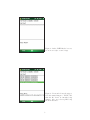
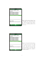
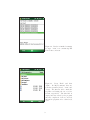
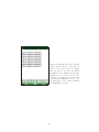
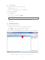
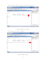
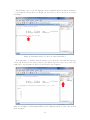
Wireless Sensing
Lab Module
Instructor’s Manual
by
Fred Schwaner, Joel Castro,
Ali Abedi, Casey Clark
Copyright 2013 – WiSe-Net Lab, ECE Dept, UMaine
Educational use of this document and associated source codes when citing
the reference is permitted.
Any other use including, but not limited to, the commercial and/or for
profit use requires licensing permission from WiSe-Net Lab Director, Dr.
Ali Abedi, [email protected]
WISENET.EECE.MAINE.EDU
1
1
Note to Instructors
This exists as a supplemental version of the standard user manual, which is also included
with this product. The purpose of this manual is to introduce you to the phenomenon of
signal fading. The MC 9090 that runs the software included with this manual is capable of
transmitting a radio frequency electromagnetic signal. Just like light, sound, and other types
of signals, electromagnetic signals fade. Fading is dependent on many factors. Among them
are distance and obstacles. This manual is to introduce you to these factors and discusses the
hardware and software used to introduce these concepts to students.
2
System Overview
The electromagnetic signal transmitted by the MC9090 is used to communicate with what
are called Radio Frequency Identification, or RFID tags. RFID tags are available in many
shapes and sizes, but all work approximately the same way. The tags consist of an antenna,
a microchip, and, sometimes, a small battery. The antenna on the tag converts the power in
the signal transmitted by the reader to electricity to power the microchip. The microchip then
sends an identification number back to the MC9090 by transmitting it on the tag’s antenna.
Small batteries are sometimes used to help power the microchip because, as you may find out,
the signal strength decreases in some situations making it more difficult to successfully read the
tag.
3
Fading
Fading is the disruption of a signal due to environmental factors. As the electromagnetic signal
propagates, its strength decays. This is not unlike any other form of signal. In fact, we deal
with this phenomenon every day whether we are aware of it or not. When we speak to one
another from longer distances we have to increase the volume of our voice. The reason for this
is that the strength of the sound coming from the other person decreases the farther the two
people are apart.
The same effect can occur due to obstacles. When there are obstacles in the way, two things
can happen. Firstly, the signal will degrade. When people speak from different rooms of a
house, the sound is often muffled and quieter due to some of the sound’s energy being absorbed
by walls and floors. Secondly, the signal can bounce. When sound reflects off multiple obstacles,
the path travelled by the signal often returns to the place of origin, resulting in an echo. This
is similar to one heard by yelling in a large empty room.
4
Experiments
Different experiments, described here, are designed to experiment with the conditions that cause
fading.
4.1
Experience Packet Loss Due to Distance
• Stand 50cm from the tag with the MC9090.
• Attempt to read the tag for a 10 seconds.
• Repeat the previous step for distances of 100cm, 150cm ...
• Count the number of successful reads, R, at each location and plot them.
1
• Attempt to match an equation of the following type to your data points:
R = T eαd
, where d is distance (in meters), α is a decay factor, T is an adjustment variable, and R
is the number of tags read at each location.
Figure 1: Distance Experiment
4.2
Experience Packet Loss Due to Obstacles
• Place a tag on a wall. Standing on the other side of the wall, attempt the same experiment
as above.
• How do the equations compare? How do T and α differ from in the previous experiment?
• Attempt this with various types of walls and objects.
• Try placing objects between you and the tag, but off to the side so the MC9090 still has
a direct path to the tag.
Figure 2: Obstacle Experiment
2
4.3
Experience Packet Loss Due to Reflections
• Place the tag on a tall, movable object 1 meter from a wall.
• Stand facing the wall, 50cm from the wall, yet off to the side, so that you are reflecting
the signal off the wall to the tag.
• Attempt to read the tag for 10 seconds.
• Repeat, while moving the tag backwards from the wall.
• Record and plot.
Figure 3: Reflection Experiment
5
MC9090 Hardware
5.1
Requirements
• Motorola MC9090 RFID Reader
• Connector cable for communication with PC
5.2
Overview
The hardware used is a Motorola MC9090-Z RFID handheld device. This is a Windows Mobile
device with IEEE 802.11a/b/g support allowing wireless networking with other computers and
wireless internet routers. The unit is controlled by an Intel XScale Bulverde PXA270 processor,
running at 624 MHz. This provides ample speed for applications and data management. The
RFID reader built into the device has an output power of 4 watts EIRP and can read tags up
to 10 feet away. The unit’s field of view is a 70 degree cone from the nose of the device. The
MC9090-Z RFID is widely available for purchase from a simple internet search.
The tags used are EPC Gen 2 RFID tags. These tags are highly compatible with most
readers as they were standardized to simplify a wide range of varying protocols used in early
RFID systems. As a result, they are very easy to work with, easy to find, and cheap to purchase.
For our development purposes, we used ALN-9634 from Alien Technologies as they offered good
angular sensitivity and were readily available.
3
6
C# Software
6.1
Requirements
• Microsoft Windows XP or newer
• Microsoft Visual Studio (2008 or later recommended)
• Windows Mobile 6 Professional Software Development Kit
• Microsoft Activesync
Note: Activesync and the Mobile 6 Professional SDK are available for free from Microsoft.
6.2
Installing the Software
The code is written in C# and can be opened using Microsoft Visual Studio. The SenseME.Mobile
solution file (.sln) is in the code’s root directory. Visual Studio lists the files used in the project
on the right hand side (by default). The main function is located in “Program.cs”. The two
windows in the program each have a designer file and a code file. The designer file simply
describes the physical setup of the window. The code file runs the features of the window.
Visual Studio also provides methods to compile, build, and install the program onto the
MC9090. In order to install, or deploy, the solution to the MC9090, one must have Microsoft
Activesync installed on their computer. Activesync allows communication between the MC9090
and the computer to allow transfer of files. Visual Studio should install the executable in the
My Devices>My Program directory of the MC9090.
The code is available for download at the WiSe-Net website.
6.3
How To Use
This program is designed to be very simple to use. Upon start, a simple “How To” procedure
is shown to the user describing, very simply, how to use the software, as shown in Figure 4.
Figure 4: Welcome Screen
4
From this screen, the user may either press “Quit” in the lower left corner or ”Begin” in the
lower right. This button leads to the RFID reading screen.
At the RFID screen, seen in Figure 5, the user may begin reading tags. A table of recentlyread tags is displayed and the RFID reader status (which can be either “Busy” or “Ready”) is
printed at the bottom of the screen.
Figure 5: RFID Reader Screen
To read tags, simply press the trigger button on the MC9090. The reader status will change
to “Busy” and below that, a message will be displayed indicating the name of a text file being
written with all the tags read.
The RFID reader scans for tags in intervals of 10 seconds. At the end of 10 seconds, the
reader will beep. If the trigger is still pressed, the user will continue reading, in 10 second
intervals, and beeping until the trigger is released and its current 10-second interval is over.
When the reader switches back to “Ready” mode, the message below the status indicator
contains the location of the file just written.
The text file written by the program includes the tag IDs of all the tags read during the
interval. The files are written into “My Documents”. Naming convention is “1.txt” for the first
reading interval, “2.txt” for the second reading interval, so on.
When the user wishes to quit the program, they may press “Back” in the lower left corner,
returning them to the welcome screen.
7
Related Reference Material
• MC9090-G Regulatory Guide
• MC9090-G RFID Integrator Guide
5
8
Illustrated Sample How-To Procedure
Figure 6: From “My Device/Program
Files/senseme.mobile.test”, open the
“SenseME.Mobile.Test” file.
Figure 7: At the welcome screen, press
“Begin” in the lower right.
6
Figure 8: At the “RFID Reader” screen,
we are now ready to scan for tags.
Figure 9: Press and release the trigger.
Note the status changes to “BUSY” and
that the file “1.txt” is currently being
written. Also, note the tag IDs being
shown in the table.
7
Figure 10: After 10 seconds, the device
beeps. Also, the status changes back
to “READY” and a message indicates
file “1.txt” has finished being written.
“1.txt” now contains tag IDs from a 10
second scan
Figure 11: Press and hold the trigger.
Notice the tag list clears and begins
to repopulate as tags are once again
recorded. After the device beeps (after 10 seconds), release the trigger. The
reader will continue to scan for tags until
the next beep, which will occur 10 seconds after the first.
8
Figure 12: Reader is finished scanning
for tags. “2.txt” now contains tag IDs
from a 20 second scan.
Figure 13:
Press “Back” and then
“Quit” . In “My Documents” there are
now three text files (“1.txt”, “2.txt”, and
“3.txt”. The first two files contain the
tag IDs read during the two read intervals, respectively. The third file is
empty, and was created by the program
after the completion of the second read
interval in preparation for a third read
cycle.
9
Figure 14: Opening file “2.txt” displays
a file counter at the top of the page, as
well as a list of the tags read. These
files can then be read into the MATLAB function for analysis and plotting.
NOTE: You can use the use the ActiveSync or Storage Device mode when
connecting the MC9090 to a PC to copy
the files created over to a PC for running
the MATLAB code later.
10
9
MATLAB Code
9.1
Requirements
• MATLAB 2009b or newer
• Directory containing only files generated by RFID Reader
• List of known test distances
9.1.1
Note on Compatibility
This MATLAB function was written for MATLAB 2009b and is guarenteed to work as described
for that and newer versions which are for the most part backwards compatible. It may also run
in older versions of MATLAB but has not been verified. This code uses only the base components installed with MATLAB and most PC’s should be capable of running a base version of
MATLAB. No special requirements are necessary for the PC specifications ouside the minimum
requirements for MATLAB itself.
9.2
Overview
This function reads the set of files containing the RFID tags read in by the MC9090 RFID
reader and plots the number of read tags for each distance. This requires the directory where
the files generated by the MC9090 code are located at and a list of the distances that the test
was conducted at. The ordered list of tags counted at each distance is created in the workspace
and a figure is plotted where the x- and y-axis represents the distance and number of packets
received, respectively.
9.3
Function Properties
As mentioned in the Overview, the function uses the directory of the files input as a string
and the distances used in the sampling as a vector. The number of distances input must not
exceed the number of files created during the test. There can be more files than distances,
however. This is allowed since the software for the RFID reader creates files before the user
starts recording; this means there will always be 1 extra but near-empty file. The function
takes the directory with the files and begins to extract the tags from each file and then save
the most common tag and the number of times it appears. This is done since it is assumed the
user was aiming directly at the desired tag and any other tags that might appear, especially at
further distances, will be read less. The function then takes these data values and sorts them
in ascending order of distance. For example:
d i s t a n c e s = [ 5 10 1 2 0 ] ;
d a t a S e t = [ 1 0 0 20 200 2 ] ;
becomes
d i s t a n c e s = [ 1 5 10 2 0 ] ;
d a t a S e t = [ 2 0 0 100 20 2 ] ;
A figure is then generated as explained in the overview. Note that the plot distances are in feet.
The code is written such that input values for distance are assumed to be in feet. This can be
changed in the plotting section of the code. Please see the comments in the MATLAB function
script for more details.
11
9.4
Use of Function
As a prerequisite, make sure the user has the following:
• MATLAB 2009b or newer
• Directory containing only files generated by RFID Reader
• List of known test distances
The procedures are simply:
1. Open MATLAB
2. Go to directory containing the file plt files.m
3. Type the command:
p l t f i l e s ( ’<d i r e c t o r y > ’ , [< d i s t a n c e s i n o r d e r >])
replacing <directory>and <distances in order>with respective values.
4. and press Enter.
10
MATLAB Example
Let us use the following as an example.
• Tag files are stored in the directory: C:\Users\Guest\Documents\data
• The plt files.m file is located in C:\Users\Guest\Documents
• The distances for the experiment were 1’, 2’, 5’, 7’, and 10’.
First, we go to file location C:\Users\Guest\Documents using the cd command in MATLAB.
Figure 15: Using the ’cd’ command to get to the proper directory.
12
You can use the ls command to check and see if the file is where it should be.
Figure 16: Results of ’ls’ command.
The command to be typed would look like this:
Figure 17: Example Command
13
An alternative can be to use the input the directory with the files as a relative path where
’./’ represents the current directory. In this case the directory can be entered as seen in the
next image.
Figure 18: Alternative method of directory entry is underlined.
It is important to remember that the distance vector is in the order that the tags were
collected in. If they are not, the plot may become distorted and out of the correct order. The
result can be seen as printed to the screen and added to the workspace.
Figure 19: Workspace and Command Window after calling the function. (Note ’ans’ is saved
in the workspace.
14
The figure generated looks like the following:
Figure 20: Plot of Received Packets versus Measured Distance
15
About Authors:
Dr. Ali Abedi is Associate Professor of Electrical and Computer Engineering and Director of
Wireless Sensor Networks (WiSe-Net) Lab, UMaine, Orono. He serves as Principal Investigator
on this project. Mr. Fred Schwaner and Mr. Joel Castro are graduate students at UMaine who
helped in developing the code and manual for this lab module. Mr. Casey Clark is an
undergraduate research assistant at UMaine who helped with preparation of this manual.
WISENET.EECE.MAINE.EDU