Download INSTITUT F¨UR INFORMATIK CASE Tools for Embedded Systems

TUM
I N S T I T U T F Ü R I N F O R M A T I K
CASE Tools for Embedded Systems
Bernhard Schätz, Tobias Hain, Frank Houdek, Wolfgang
Prenninger, Martin Rappl,Jan Romberg, Oscar Slotosch,
Martin Strecker, Alexander Wisspeintner
TUM-I0309
Juli 03
T E C H N I S C H E U N I V E R S I T Ä T M Ü N C H E N
TUM-INFO-07-I0309-0/1.-FI
Alle Rechte vorbehalten
Nachdruck auch auszugsweise verboten
c 2003
Druck:
Institut für Informatik der
Technischen Universität München
CASE Tools for Embedded
Systems1
Bernhard Schätz, Tobias Hain, Frank Houdek,
Wolfgang Prenninger, Martin Rappl, Jan Romberg,
Oscar Slotosch, Martin Strecker, Alexander Wisspeintner
and contributions by
Christoph Angerer, Martin Glaser, Christian Merenda,
Josef Maran, Martin Mössmer, Jürgen Steurer,
Percy Stocker, Armin Fischer, Stefan Gersmann,
Maria Bozo, Karin Katheder, Thomas Off,
Bastian Best, Julian Broy, Gerrit Hanselman, Peggy Sekatzek
Anis Trimeche, Abdellatif Zaouia, Hongkun Jiang
Karin Beer, Christian Truebswetter, Alexander Woitala,
Clemens Lanthaler, Petr Ossipov, Tania Fichtner
July 24, 2003
1
This work was in part supported by the DFG (projects KONDISK/IMMA,
InOpSys, Inkrea„ and SPP 1040 under reference numbers Be 1055/7-3, Br 887/161, and Br 887/14-1, Br 887/9, and InTime (SPP 1064)).
2
Contents
1
Introduction
1.1 Overview . . . . . . . . . . . . . . . .
1.2 What This Report Does Not Aim At
1.3 What This Report Does Aim At . . .
1.4 Acknowledgments . . . . . . . . . .
.
.
.
.
.
.
.
.
.
.
.
.
.
.
.
.
.
.
.
.
.
.
.
.
.
.
.
.
.
.
.
.
.
.
.
.
.
.
.
.
.
.
.
.
.
.
.
.
.
.
.
.
.
.
.
.
9
10
10
11
11
I
Preface
2
Assessing the Tools
2.1 General Aspects . . . . . . . . . . . . . . .
2.2 Modeling the System . . . . . . . . . . . .
2.2.1 Available Description Techniques
2.2.2 Applied Description Techniques .
2.2.3 Complexity of Description . . . . .
2.2.4 Operational Model . . . . . . . . .
2.3 Development Process . . . . . . . . . . . .
2.3.1 Applied Process . . . . . . . . . . .
2.3.2 Applied Process Support . . . . .
2.3.3 Applied Quality Management . .
2.3.4 Applied Target Platform . . . . . .
2.3.5 Incremental Development . . . . .
2.4 Conclusion . . . . . . . . . . . . . . . . . .
2.5 Model of the Controller . . . . . . . . . . .
.
.
.
.
.
.
.
.
.
.
.
.
.
.
.
.
.
.
.
.
.
.
.
.
.
.
.
.
.
.
.
.
.
.
.
.
.
.
.
.
.
.
.
.
.
.
.
.
.
.
.
.
.
.
.
.
.
.
.
.
.
.
.
.
.
.
.
.
.
.
.
.
.
.
.
.
.
.
.
.
.
.
.
.
.
.
.
.
.
.
.
.
.
.
.
.
.
.
.
.
.
.
.
.
.
.
.
.
.
.
.
.
.
.
.
.
.
.
.
.
.
.
.
.
.
.
.
.
.
.
.
.
.
.
.
.
.
.
.
.
.
.
.
.
.
.
.
.
.
.
.
.
.
.
15
15
16
16
17
17
18
18
19
19
20
20
21
21
21
Result Summary
3.1 General Aspects . . . . . . . . . . . . . . .
3.1.1 Functionality . . . . . . . . . . . .
3.1.2 Development Process . . . . . . .
3.1.3 Documentation . . . . . . . . . . .
3.1.4 Usability . . . . . . . . . . . . . . .
3.2 Modeling the System . . . . . . . . . . . .
3.2.1 Available Description Techniques
.
.
.
.
.
.
.
.
.
.
.
.
.
.
.
.
.
.
.
.
.
.
.
.
.
.
.
.
.
.
.
.
.
.
.
.
.
.
.
.
.
.
.
.
.
.
.
.
.
.
.
.
.
.
.
.
.
.
.
.
.
.
.
.
.
.
.
.
.
.
.
.
.
.
.
.
.
23
23
23
25
25
26
26
27
3
13
3
CONTENTS
4
.
.
.
.
.
.
.
.
.
.
28
29
30
33
34
35
37
39
39
40
Model-Based Development
Bibliography . . . . . . . . . . . . . . . . . . . . . . . . . . . . . . .
43
47
3.3
3.4
4
II
5
6
3.2.2 Applied Description Techniques
3.2.3 Complexity of Description . . . .
3.2.4 Operational Model . . . . . . . .
Development Process . . . . . . . . . . .
3.3.1 Applied Process . . . . . . . . . .
3.3.2 Applied Process Support . . . .
3.3.3 Applied Quality Management .
3.3.4 Applied Target Platform . . . . .
3.3.5 Incremental Development . . . .
Conclusion . . . . . . . . . . . . . . . . .
.
.
.
.
.
.
.
.
.
.
.
.
.
.
.
.
.
.
.
.
.
.
.
.
.
.
.
.
.
.
.
.
.
.
.
.
.
.
.
.
.
.
.
.
.
.
.
.
.
.
.
.
.
.
.
.
.
.
.
.
.
.
.
.
.
.
.
.
.
.
.
.
.
.
.
.
.
.
.
.
.
.
.
.
.
.
.
.
.
.
.
.
.
.
.
.
.
.
.
.
.
.
.
.
.
.
.
.
.
.
The Tools
49
Tool ARTiSAN RealTime Studio
5.1 General Aspects . . . . . . . . . . . . . . .
5.1.1 Functionalities . . . . . . . . . . .
5.1.2 Development phases . . . . . . . .
5.1.3 Documentation . . . . . . . . . . .
5.1.4 Usability . . . . . . . . . . . . . . .
5.2 Modeling the system . . . . . . . . . . . .
5.2.1 Available Description Techniques
5.2.2 Applied Description Techniques .
5.2.3 Complexity of description . . . . .
5.2.4 Modeling Interaction . . . . . . . .
5.3 Development Process . . . . . . . . . . . .
5.3.1 Applied Process . . . . . . . . . . .
5.3.2 Process Support . . . . . . . . . . .
5.3.3 Applied quality management . . .
5.3.4 Applied Target Plattform . . . . .
5.3.5 Incremental Development . . . . .
5.4 Conclusion . . . . . . . . . . . . . . . . . .
5.5 Model of the Controller . . . . . . . . . . .
5.5.1 Description of the structure . . . .
5.5.2 Description of the functionality . .
.
.
.
.
.
.
.
.
.
.
.
.
.
.
.
.
.
.
.
.
.
.
.
.
.
.
.
.
.
.
.
.
.
.
.
.
.
.
.
.
.
.
.
.
.
.
.
.
.
.
.
.
.
.
.
.
.
.
.
.
.
.
.
.
.
.
.
.
.
.
.
.
.
.
.
.
.
.
.
.
.
.
.
.
.
.
.
.
.
.
.
.
.
.
.
.
.
.
.
.
.
.
.
.
.
.
.
.
.
.
.
.
.
.
.
.
.
.
.
.
.
.
.
.
.
.
.
.
.
.
.
.
.
.
.
.
.
.
.
.
.
.
.
.
.
.
.
.
.
.
.
.
.
.
.
.
.
.
.
.
.
.
.
.
.
.
.
.
.
.
.
.
.
.
.
.
.
.
.
.
.
.
.
.
.
.
.
.
.
.
.
.
.
.
.
.
.
.
.
.
.
.
.
.
.
.
.
.
.
.
.
.
.
.
.
.
.
.
.
.
51
51
51
52
52
53
53
53
57
59
59
60
60
61
62
63
64
65
65
66
66
Ascet-SD
6.1 General Aspects . . . . . . . . . . . . . . .
6.2 Modelling the System . . . . . . . . . . . .
6.2.1 Available Description Techniques
6.2.2 Applied Description Techniques .
.
.
.
.
.
.
.
.
.
.
.
.
.
.
.
.
.
.
.
.
.
.
.
.
.
.
.
.
.
.
.
.
.
.
.
.
.
.
.
.
.
.
.
.
73
73
75
75
81
CONTENTS
.
.
.
.
.
.
.
.
.
.
.
.
.
.
.
.
.
.
.
.
.
.
.
.
.
.
.
.
.
.
.
.
.
.
.
.
.
.
.
.
.
.
.
.
.
.
.
.
.
.
.
.
.
.
.
.
.
.
.
.
.
.
.
.
.
.
.
.
.
.
.
.
.
.
.
.
.
.
.
.
.
.
.
.
.
.
.
.
.
.
.
.
.
.
.
.
.
.
.
.
.
.
.
.
.
.
.
.
.
.
.
.
.
.
.
.
.
.
.
.
.
.
.
.
.
.
.
.
.
.
.
.
.
.
.
.
.
.
.
.
.
.
.
. 82
. 82
. 84
. 84
. 84
. 86
. 88
. 89
. 90
. 91
. 91
. 95
. 100
AutoFocus
7.1 General Aspects . . . . . . . . . . . . . . .
7.2 Modeling the sytem . . . . . . . . . . . . .
7.2.1 Available Description Techniques
7.2.2 Applied Description Techniques .
7.2.3 Complexity of Description . . . . .
7.2.4 Modeling Interaction . . . . . . . .
7.3 Development Process . . . . . . . . . . . .
7.3.1 Applied Process . . . . . . . . . . .
7.3.2 Applied Process Support . . . . .
7.3.3 Applied Quality Management . .
7.3.4 Applied Target Platform . . . . . .
7.3.5 Incremental Development . . . . .
7.4 Model of the Controller . . . . . . . . . . .
7.4.1 Door Control . . . . . . . . . . . .
7.4.2 Seat Control . . . . . . . . . . . . .
7.4.3 User Control . . . . . . . . . . . . .
7.4.4 Merger . . . . . . . . . . . . . . . .
7.5 Conclusion . . . . . . . . . . . . . . . . . .
7.5.1 Benefits . . . . . . . . . . . . . . .
7.5.2 Weaknesses . . . . . . . . . . . . .
7.5.3 Desired features . . . . . . . . . . .
.
.
.
.
.
.
.
.
.
.
.
.
.
.
.
.
.
.
.
.
.
.
.
.
.
.
.
.
.
.
.
.
.
.
.
.
.
.
.
.
.
.
.
.
.
.
.
.
.
.
.
.
.
.
.
.
.
.
.
.
.
.
.
.
.
.
.
.
.
.
.
.
.
.
.
.
.
.
.
.
.
.
.
.
.
.
.
.
.
.
.
.
.
.
.
.
.
.
.
.
.
.
.
.
.
.
.
.
.
.
.
.
.
.
.
.
.
.
.
.
.
.
.
.
.
.
.
.
.
.
.
.
.
.
.
.
.
.
.
.
.
.
.
.
.
.
.
.
.
.
.
.
.
.
.
.
.
.
.
.
.
.
.
.
.
.
.
.
.
.
.
.
.
.
.
.
.
.
.
.
.
.
.
.
.
.
.
.
.
.
.
.
.
.
.
.
.
.
.
.
.
.
.
.
.
.
.
.
.
.
.
.
.
.
.
.
.
.
.
.
.
.
.
.
.
.
.
.
.
.
.
101
101
102
102
104
105
106
107
107
108
110
112
112
113
114
118
119
120
120
120
121
121
MATLAB/Stateflow
8.1 General Aspects . . . . . . . . . . . . . . .
8.2 Modeling the System . . . . . . . . . . . .
8.2.1 Available Description Techniques
8.2.2 Applied Description Techniques .
8.2.3 Complexity of Description . . . . .
8.2.4 Modeling Interaction . . . . . . . .
.
.
.
.
.
.
.
.
.
.
.
.
.
.
.
.
.
.
.
.
.
.
.
.
.
.
.
.
.
.
.
.
.
.
.
.
.
.
.
.
.
.
.
.
.
.
.
.
.
.
.
.
.
.
.
.
.
.
.
.
.
.
.
.
.
.
123
123
125
125
127
128
128
6.3
6.4
6.5
7
8
6.2.3 Complexity of Description . . .
6.2.4 Modelling Interaction . . . . .
Development Process . . . . . . . . . .
6.3.1 Applied Process . . . . . . . . .
6.3.2 Applied Process Support . . .
6.3.3 Applied Quality Management
6.3.4 Applied Target Platform . . . .
6.3.5 Incremental Development . . .
Conclusion . . . . . . . . . . . . . . . .
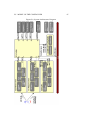
Model of the Controller . . . . . . . . .
6.5.1 Structure . . . . . . . . . . . . .
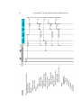
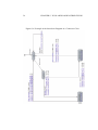
6.5.2 Functionality . . . . . . . . . .
6.5.3 Attachment . . . . . . . . . . .
5
.
.
.
.
.
.
.
.
.
.
.
.
.
CONTENTS
6
8.3
8.4
8.5
8.6
9
Development Process . . . . . . . . . . . . .
8.3.1 Applied Process . . . . . . . . . . . .
8.3.2 Applied Process Support . . . . . .
8.3.3 Applied Quality Management . . .
8.3.4 Incremental Development . . . . . .
Conclusion . . . . . . . . . . . . . . . . . . .
Model of the Controller . . . . . . . . . . . .
8.5.1 Overview . . . . . . . . . . . . . . .
8.5.2 Components and their Functionality
8.5.3 Tests . . . . . . . . . . . . . . . . . .
Appendix: Faults in the specification . . . .
.
.
.
.
.
.
.
.
.
.
.
.
.
.
.
.
.
.
.
.
.
.
.
.
.
.
.
.
.
.
.
.
.
.
.
.
.
.
.
.
.
.
.
.
.
.
.
.
.
.
.
.
.
.
.
.
.
.
.
.
.
.
.
.
.
.
.
.
.
.
.
.
.
.
.
.
.
.
.
.
.
.
.
.
.
.
.
.
.
.
.
.
.
.
.
.
.
.
.
.
.
.
.
.
.
.
.
.
.
.
130
130
131
132
134
135
136
136
136
149
153
Rhapsody in MicroC
9.1 General Aspects . . . . . . . . . . . . . . .
9.2 Modelling the System . . . . . . . . . . . .
9.2.1 Available Description Techniques
9.2.2 Applied Description Techniques .
9.2.3 Complexity of Description . . . . .
9.2.4 Modelling Interaction . . . . . . .
9.3 Development Process . . . . . . . . . . . .
9.3.1 Applied Process . . . . . . . . . . .
9.3.2 Applied Process Support . . . . .
9.3.3 Applied Quality Management . .
9.3.4 Applied Target Platform . . . . . .
9.3.5 Incremental Development . . . . .
9.4 Conclusion . . . . . . . . . . . . . . . . . .
9.5 Model of the Controller . . . . . . . . . . .
.
.
.
.
.
.
.
.
.
.
.
.
.
.
.
.
.
.
.
.
.
.
.
.
.
.
.
.
.
.
.
.
.
.
.
.
.
.
.
.
.
.
.
.
.
.
.
.
.
.
.
.
.
.
.
.
.
.
.
.
.
.
.
.
.
.
.
.
.
.
.
.
.
.
.
.
.
.
.
.
.
.
.
.
.
.
.
.
.
.
.
.
.
.
.
.
.
.
.
.
.
.
.
.
.
.
.
.
.
.
.
.
.
.
.
.
.
.
.
.
.
.
.
.
.
.
.
.
.
.
.
.
.
.
.
.
.
.
.
.
.
.
.
.
.
.
.
.
.
.
.
.
.
.
155
155
158
158
163
163
164
165
165
165
167
169
170
170
172
10 Rational Rose RealTime
10.1 General Aspects . . . . . . . . . . . . . . .
10.2 Modeling the System . . . . . . . . . . . .
10.2.1 Available Description Techniques
10.2.2 Applied Description Techniques .
10.2.3 Complexity of Description . . . . .
10.2.4 Modeling Interaction . . . . . . . .
10.3 Development Process . . . . . . . . . . . .
10.3.1 Applied Process . . . . . . . . . . .
10.3.2 Applied Process Support . . . . .
10.3.3 Applied Quality Management . .
10.3.4 Applied Target Platform . . . . . .
10.3.5 Incremental Development . . . . .
10.4 Conclusion . . . . . . . . . . . . . . . . . .
10.5 Model of the Controller . . . . . . . . . . .
10.5.1 TSG Design . . . . . . . . . . . . .
.
.
.
.
.
.
.
.
.
.
.
.
.
.
.
.
.
.
.
.
.
.
.
.
.
.
.
.
.
.
.
.
.
.
.
.
.
.
.
.
.
.
.
.
.
.
.
.
.
.
.
.
.
.
.
.
.
.
.
.
.
.
.
.
.
.
.
.
.
.
.
.
.
.
.
.
.
.
.
.
.
.
.
.
.
.
.
.
.
.
.
.
.
.
.
.
.
.
.
.
.
.
.
.
.
.
.
.
.
.
.
.
.
.
.
.
.
.
.
.
.
.
.
.
.
.
.
.
.
.
.
.
.
.
.
.
.
.
.
.
.
.
.
.
.
.
.
.
.
.
.
.
.
.
.
.
.
.
.
.
.
.
.
.
.
179
179
180
180
187
188
189
190
190
190
192
193
194
194
195
196
CONTENTS
7
10.5.2 Komponenten Design . . . . . . . . . . . . . . . . . . 196
10.5.3 Object Model . . . . . . . . . . . . . . . . . . . . . . . 200
11 Telelogic Tau
11.1 General Aspects . . . . . . . . . . . . . . .
11.2 Modeling the System . . . . . . . . . . . .
11.2.1 Available Description Techniques
11.2.2 Applied Description Techniques .
11.2.3 Complexity of Description . . . . .
11.2.4 Modeling Interaction . . . . . . . .
11.3 Development Process . . . . . . . . . . . .
11.3.1 Applied Process . . . . . . . . . . .
11.3.2 Applied Process Support . . . . .
11.3.3 Applied Quality Management . .
11.3.4 Applied Target Platform . . . . . .
11.3.5 Incremental Development . . . . .
11.4 Conclusion . . . . . . . . . . . . . . . . . .
11.5 Model of the Controller . . . . . . . . . . .
11.5.1 Packages and Classes . . . . . . .
11.5.2 Architecture . . . . . . . . . . . . .
11.5.3 Design of the behavior . . . . . . .
.
.
.
.
.
.
.
.
.
.
.
.
.
.
.
.
.
.
.
.
.
.
.
.
.
.
.
.
.
.
.
.
.
.
.
.
.
.
.
.
.
.
.
.
.
.
.
.
.
.
.
.
.
.
.
.
.
.
.
.
.
.
.
.
.
.
.
.
.
.
.
.
.
.
.
.
.
.
.
.
.
.
.
.
.
.
.
.
.
.
.
.
.
.
.
.
.
.
.
.
.
.
.
.
.
.
.
.
.
.
.
.
.
.
.
.
.
.
.
.
.
.
.
.
.
.
.
.
.
.
.
.
.
.
.
.
.
.
.
.
.
.
.
.
.
.
.
.
.
.
.
.
.
.
.
.
.
.
.
.
.
.
.
.
.
.
.
.
.
.
.
.
.
.
.
.
.
.
.
.
.
.
.
.
.
.
.
201
201
202
202
208
210
212
214
214
214
217
219
220
220
221
221
223
225
12 Trice Tool by Protos Software GmbH
12.1 General Aspects . . . . . . . . . . . . . . .
12.2 Modeling the System . . . . . . . . . . . .
12.2.1 Available Description Techniques
12.2.2 Applied Description Techniques .
12.2.3 Complexity of Description . . . . .
12.2.4 Modeling Interaction . . . . . . . .
12.3 Development Process . . . . . . . . . . . .
12.3.1 Applied Process . . . . . . . . . . .
12.3.2 Applied Process Support . . . . .
12.3.3 Applied Quality Management . .
12.3.4 Applied Target Platform . . . . . .
12.3.5 Incremental Development . . . . .
12.4 Conclusion . . . . . . . . . . . . . . . . . .
12.5 Model of the Controller . . . . . . . . . . .
.
.
.
.
.
.
.
.
.
.
.
.
.
.
.
.
.
.
.
.
.
.
.
.
.
.
.
.
.
.
.
.
.
.
.
.
.
.
.
.
.
.
.
.
.
.
.
.
.
.
.
.
.
.
.
.
.
.
.
.
.
.
.
.
.
.
.
.
.
.
.
.
.
.
.
.
.
.
.
.
.
.
.
.
.
.
.
.
.
.
.
.
.
.
.
.
.
.
.
.
.
.
.
.
.
.
.
.
.
.
.
.
.
.
.
.
.
.
.
.
.
.
.
.
.
.
.
.
.
.
.
.
.
.
.
.
.
.
.
.
.
.
.
.
.
.
.
.
.
.
.
.
.
.
227
227
229
229
230
231
231
232
232
232
234
235
236
237
238
III
Requirement Specification of the Controller
13 Das Türsteuergerät - eine Beispielspezifikation
247
249
8
CONTENTS
Chapter 1
Introduction
In this report, we show how eight different CASE tools for embedded systems can be used to develop the model of controller software for comfort
electronic in the automotive domain. The applied tools are
• ARTiSAN RealTime Studio by Artisan Software
• ASCET-SD by ETAS GmbH & Co.KG
• AutoF OCUS by Technische Universität München
• MATLAB/StateFlow by The MathWorks Inc.
• Rose RealTime by Rational
• Rhapsody in MicroC by I-Logix Inc.
• Telelogic Tau G2 by Telelogic Inc.
• Trice Tool by Protos Software GmbH
With each tool, a model of a controller software module was developed,
based on a given textual requirement specification. The requirement specification of the controller was taken from a revised version of a controller
specification provided by F. Houdek, Daimler Chrysler AG. Each tool was
applied by a group of three to four students; the students had no experience
with the applied tool. After receiving an initial training in using the tool,
the students were given three months to develop the model. The model of
the controller software was developed in two steps (first step: simplified
three axis seat control; second step: five axis seat control) to add the aspect
of specification reuse. Finally, the application of the tool was assessed by
each team using a common questionnaire.
This report presents the results of these questionnaires in a detail, and
summarizes them to give a "state of the art" impression of CASE tools for
embedded systems. Building on this summary, it sketches what properties
9
CHAPTER 1. INTRODUCTION
10
are necessary to extend this "state of the art" into a model-based development process.
1.1
Overview
The report consists of three parts:
Preface: In the first part we describe the questionnaire used to asses the
tools (Chapter 2), give a short summary of the results (Chapter 3), and
sketch what is to be expected from model-based CASE support in the
future (Chapter 4).
Tools: In the second part for each tool we include the results as described
by the students:
• ARTiSAN RealTime Studio (Chapter 5)
• ASCET-SD (Chapter 6)
• AutoF OCUS (Chapter 7)
• MATLAB/StateFlow (Chapter 8)
• Rhapsody in MicroC (Chapter 9)
• Rose RealTime (Chapter 10)
• Telelogic Tau G2 (Chapter 11)
• Trice Tool by (Chapter 12)
Requirement Specification: In the last part, we include the requirement
specification as used in the case study.
1.2
What This Report Does Not Aim At
The case study focuses on the use of CASE tools for the specification of embedded software. Therefore, several aspects essential to the development
of embedded systems are not sufficiently addressed to supply a complete
and sufficiently detailed picture of the tools. These aspects include
• Ease of deployment to specific operating systems
• Ease of deployment to hardware platforms
• Memory and processor efficiency of the generated code
• Integration in a tool chain
• Availability of rapid prototyping environment
1.3. WHAT THIS REPORT DOES AIM AT
11
Accordingly, this report is not meant to be a recommendation to select a
development tool for a specific application domain. Furthermore, since
those tools do target different development phases, different application
domains as well as different development techniques, it is paramount to
select the tool that fits best into the desired development process. Thus,
while the following overview can help to get a first impression of the relevant aspects of a tool as well as the state of the art in CASE tool support,
this study cannot replace a profound tool selection depending on a thorough definition of the requirements of the tool users.
1.3
What This Report Does Aim At
The case study shows what modeling concepts are reasonable and can be
useful in the domain of embedded systems. It also shows that general purpose object-oriented modeling is not desirable in this domain; suitable tools
have to address issues like
• describing structures more abstractly than on the level of class/object
diagrams
• introducing communication mechanisms more suitable than method
or procedure calls
• modeling reactive behavior as well as data flow
Furthermore, we show what models and description techniques are commonly accepted as essential, giving a state-of-the-art snapshot of the CASEbased specification of embedded software. Additionally, we show what
kind of tool support is available for the development of such specifications
and what the resulting development process looks like with a focus on the
design phase. Finally, we sketch what should be expected from future tools
by giving a vision of model-based development of embedded software.
1.4
Acknowledgments
The assessment of the state of the art in CASE tools for embedded systems
would not have been possible without access to a representative collection
of those tools. We are therefore especially thankful for the personal commitment of the vendors and distributors through their representatives not
only in supplying us with free trial versions, but also in supplying the students with an introductory course as well as valuable feedback during the
construction of the models:
• Andreas Korff from Artisan Software for ARTiSAN RealTime Studio
CHAPTER 1. INTRODUCTION
12
• Ulrich Freund from ETAS GmbH & Co.KG for ASCET-SD
• Validas AG for AutoF OCUS support
• Andreas Goser from The MathWorks Inc. for MATLAB/StateFlow
• Rainer Hochecker and Hans Windpassinger from Rational for Rose
RealTime
• Peter Schedl and Carsten Sbick from Berner & Mattner for Rhapsody
in MicroC
• Wolfgang Sonntag from Telelogic Inc. for Telelogic Tau G2
• Klaus Birken from Protos Software GmbH for Trice Tool
Part I
Preface
13
Chapter 2
Assessing the Tools
Bernhard Schätz, Tobias Hain, Wolfgang Prenninger,
Martin Rappl, Jan Romberg, Oscar Slotosch,
Martin Strecker, Alexander Wisspeintner
While all of the tools discussed in the sections of the second part support
the development of reactive software systems, they differ concerning how
specifically they address the development of embedded software. As a result, they focus on different aspects of the development process, e.g., modeling the system under development, supporting the test of the system, or
generating and deploying code to the embedded controller. Therefore, to
simplify a comparison of the different functionalities offered by the tools,
the tools were analyzed according to different criteria, which we present in
a structured format in the following sections.
After giving a short overview of each tool, the modeling concepts of the
tool – as applied in the case study – are discussed, focusing on its description techniques, the complexitiy of the resulting description of the system,
and the interpretation (i.e., the operational model) behind those description techniques. In the next section, the process support offered by the tool
is discussed, specifically addressing issues concerning functionalities supporting the modeling of the system, qualitiy assurance, deployment, and
incremental development. After a short conclusion – giving a short summary of the tool as well as some of its pros and cons – the model of the
controller as developed using the tool is illustrated in detail.
For each of the sections, a list of questions is defined to illustrate the
functionalities of the analysed tools. In the following, the sections mentioned above including their corresponding questions are listed.
2.1
General Aspects
In this section, general information about the tool is provided:
15
16
CHAPTER 2. ASSESSING THE TOOLS
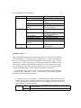
Functionalities. Which functionalities are supported by the tool (e.g. modeling, simulation, documentation, configuration management, test management, test case generation, model validation and verification.).
Development phases. During which development phases the tool can be
used (requirements analysis, design, implementation, test, deployment)?
Documentation. How good is the documentation of the tool functionalities (differ between manual and online help system) (very good, good,
satisfactory, enough, inadequate)?
Usability. How good is the usability / user interface of the tool (very good,
good, satisfactory, enough, inadequate)?
2.2
Modeling the System
This section provides information on how a system is modeled using the
description techniques supplied by the tool. Special emphasis is laid on
what kind of concepts and notions are applied to model a system, how
complex the resulting descriptions are, and what kind of operational model
is used to interpret the description. In each subsection, examples from the
modeled CASE study are used to illustrate the answers whereever suitable/possible.
2.2.1
Available Description Techniques
This subsection lists the notations and concepts provided by the tool:
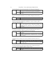
Supported notations. Which notations / constructs / diagram types are
offered by the tool (e.g. class diagrams, state machines, sequence diagrams)?
Modeling aspects. Which aspects can be modeled using the notations (according to the tool vendor) (e.g. behavior, structure, interfaces, interaction)?
Type of notation. What is the representation type of the notations (e.g.,
tabular, text, graphic)?
Hierarchy. Does the notation support hierarchical structuring (e.g., component/subcomponents, state/substates)?
2.2. MODELING THE SYSTEM
2.2.2
17
Applied Description Techniques
Approaches with a large variety of description techniques often offer different notations to describe similar or overlapping aspects (e.g., Collaboration
Diagrams and Sequence Diagrams in UML). Since in those approaches not
always all notations are applied, this section focusses on the description
technqiues applied in the case study:
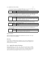
Applied notations. Which notations / constructs / diagram types have
been used during modeling the case study?
Modeled aspects. Which aspects have been modeled? (real application)
(e.g. behavior, structure, interfaces, interaction)?
Notations suitable. Are the notations suitable for modeling the case study?
Clearness. Do the notations allow to build clear and readable models?
Unused notations. Which notations / constructs / diagram types have not
been used for modeling the case study (reason)?
Missing notations. Which notations were missing while working on the
case study and what would have been modeled using these notations
(e.g. behavior, structure, interfaces, interaction)?
2.2.3
Complexity of Description
This section provides an estimation of the size of the built model. Only the
part of the specification used for executing the model (simulation / code
generation) is considered (e.g., sequence diagrams and use-case diagrams
are not considered). Since tools generally use graph-like diagrams to model
a system, a diagram-based metric for the complexitiy of the model is used.
Basis for the metric are the notions view (e.g. diagrams drawn), node (e.g.
block, component, class, state used in a diagram), edge (e.g. association,
channel, transition used in a diagram), visible annotation (text visible in
the diagrams) and invisible annotation (text hidden in dialog boxes):
Views. How many views are used in the whole model?
Nodes. How many nodes are used in the whole model? How many nodes
are user per view (average and maximum)?
Edges. How many edges are used in the whole model? How many edges
are user per view (average and maximum)?
Visible annotations. Size of the visible annotations per view (maximum
measured in characters)?
Invisible annotations. Size of the invisible annotations per view (maximum measured in characters)?
CHAPTER 2. ASSESSING THE TOOLS
18
2.2.4
Operational Model
Obviously, the choice of the operational model used to interpret the diagrams influences the complexity of the description. E.g., a operational
model supporting buffered communication can simplify the description of
a message handling strategy. In this section a short description of the operational model underlying the tool is given:
Supported communication model Which communication models are supported by the tool?
• Synchronization concerning event-scheduling:
– I/O synchronous (input and output can occur during the
same clock cycle)
– clock synchronous (all entities interact within the same clock
cycle)
– unsynchronized/event driven
– other
• Shared variables vs. messages
• Buffering: message synchronous (handshake/blocking (synchron)
vs. non-blocking, usually buffered (asynchronous) )
Communication model suitable Are the notations/the modeling techniques
suitable for modeling the case study?
Timing constraints Which notations are provided to model timing constraints?
Sufficient realtime support Is the realtime support sufficient for modeling
the case study?
2.3
Development Process
While the previous section focussed on what the model of a system looks
like, this section rather addresses the question how such a model is built.
In the following subsections, the development process is sketched and a
short description of the features (process and quality management support,
target platform) is given that were applied in the case study. Furthermore,
some of the additional features not used but offered by the tool are noted
including why they were not used (a possible reason is of course, that these
feature were not needed in the case study, especially in the target platform
section). Finally, the support for incremental development is addressed.
2.3. DEVELOPMENT PROCESS
2.3.1
19
Applied Process
This subsection gives a short summary of the development as performed
in the case study. For example, it is described the development process
is started (defining system boundries, describing initial use cases), how
model of the system is obtained (refining use cases by sequence diagrams,
defining data structures), as well as which further steps were applied (simulation, checks, test, etc.)
2.3.2
Applied Process Support
Here, all aspects that aid during the development process are listed, especially, addressing the question how much a tool has helped to understand
the specification and whether the tool supports to get models with different degrees of detail (starting with a coarse model, doing early simulations,
etc):
Simple development operations. Does the tool provide simple development operations (e.g. cut and paste of parts of a diagram)? If yes,
which operations are supported?
Complex development operations. Does the tool provide complex development operations (e.g. calculation of scheduling, protocol integration, partitioning on hardware components)? If yes, which operations
are supported?
Reverse engineering. Is reverse engineering supported by the tool (generation of diagrams out of source code)?
User support. Does the tool provide user support in form of wizards, context dependant process activities or design guidelines?
Consistency ensurance mechanisms. Does the tool offer consistency ensurance mechanisms (Mechanisms to find errors in the model)? If
yes, which kind of consistency is considered?
• syntactic consistency: e.g. type correctness, unambiguousness
of identifiers, executability.
• semantic consistency: e.g. compliance between the sequence diagrams and the state machines.
Component library. Does the tool support the usage of predefined components (e.g. clock, bus)? Is a predefined component library available?
Is the library user extensible?
Development history. Does the tool record the development history? Is it
possible to recover old development states?
20
2.3.3
CHAPTER 2. ASSESSING THE TOOLS
Applied Quality Management
Here, all performed validation and verification tasks are included that ensure that the model is correct with respect to the specification. In case faults
in the specification (inconsistencies or incompletenesses) where detected,
the faults are describes and the resolution is sketched. Additionally, the
tool is characterized along the following criteria for quality management:
Host Simulation Support. Does the tool support simulation on the PC or
workstation used for development (host)?
Target Simulation Support. Do the tools support simulation on the target
hardware? Are all the features of host simulation available?
Adequacy. How adequate are the simulation mechanisms? (e.g: numeric
simulation by curves/graphics instead of tables)
Debugging Features. Which features are available? Examples are Breakpoints, Event injection, Run-time display of variables. Debugging at
model level or code level?
Testing. How does the tool support testing? Can test vectors be played
into the model? Can test vectors be generated from models? Are
there further analysis capabilities? Are there interfaces to other test
tools? (e.g. Rational Test RealTime)
Certification Are code generators certified by an independent certification
authority? For simulation code? For target code? Are there any certified code generators available?
Requirements tracing Does the tool support tracing of requirements in the
development process? Are there interfaces to requirements engineering tools (e.g. RequisitePro, DOORS, MS Word)?
2.3.4
Applied Target Platform
Since code was not deployed in his case study, this section gives only a
short overview about the code generated out of the model of the system:
Target code generation. Does the tool support code generation for specific
target micro controllers?
Supported targets. Which target plattforms (micro controllers, operating
systems) are supported by the tool?
Code size. What is code size of the generated code for the target platform
(lines of code in C or Assembler / bytes of machine code / bytes of
used memory)?
2.4. CONCLUSION
21
Readability of code. How good is the readability of the generated target
code? Does the generated code relate to the model structure?
2.3.5
Incremental Development
This section discusses how much the tool aids in the incremental development process (i.e., going from a two-axes system to the five-axes-version):
Reuse. How much of the original specification could be reused?
Restricted changes. Could changes be restricted to a small part of the specification?
Modular design. Did the tool/approach help building a modular design
or was a very modular structure found uninfluenced by the approach
in the first stage?
Restructuring. Did the tool support restructuring techniques (e.g. refactoring)?
2.4
Conclusion
Here, a short summary of the strengths and weaknesses of the tool and its
application is given, especailly addressing the questions of what has been
missing and what was very helpful in the development.
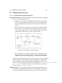
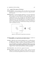
2.5
Model of the Controller
Finally, a description of the model is given, including
• a short description of the structure (what are the main modules/components,
etc)
• a short description of the functionality of each module/component
If possible, original documents generated with the tool are included. If
reasonable, also documentations of simulation protocols etc. are included,
which help to document the correctness of the model.
22
CHAPTER 2. ASSESSING THE TOOLS
Chapter 3
Result Summary
Bernhard Schätz, Jan Romberg, Oscar Slotosch, Martin Strecker
While all the discussed tools are treated in detail in the second part, in
this chapter we give a short overall summary of the tools. The aim of this
section is not to give a detailed comparison between the tools; rather, we
want to show the capabilities of tool-based development as presented by
the selected tools.
The discussed tools form a rather representative selection of the available tools for the development of embedded systems. Therefore, this summary also gives a snapshot of the state of the art of tool support for this
domain.
3.1
General Aspects
Like in other domains of CASE tool support, tools for the development
of embedded software have made significant progress concerning general
aspects including offered functionalities, supported development phases,
documentation of the tool, and their usability; unsurprisingly, all tools have
some potential for improvement. Most noticeable, CASE tools have made
strong improvements in usability, but also aspects of functionality like the
quality of the generated code, offered consistency checks, simulation, and
test automation.
3.1.1
Functionality
From a very abstract point of view, the functionalities of the tools are quite
similar. The spectrum of supported functionalities includes
• the design of the software using graphical description techniques,
• some form of analysis to detect inconsistencies,
23
CHAPTER 3. RESULT SUMMARY
24
• the possibility to simulate the design software,
• the generation of code (or code fragments) from the design, and
• the generation of documentation.
On a closer look, however, the tools differ noticeably concerning supported
description techniques, support for developing and analyzing the design,
the support for generating deployable code, or generated documentation.
Roughly, the used description techniques can be divided into two classes:
one supporting large parts of UML, the other mainly centered around the
real-time subset (block diagrams and state transition diagrams). Section 3.2
treats this in more detail.
Due to the complexity of the complete development process, the investigated tools obviously cannot cover the complete development process.
Therefore, an important aspect of the tools is their integration in the development in terms of interfaces to other development tools (e.g., tools for
requirements elicitation and analysis, configuration management, or regression test). While some tools offered only support to import and export models, others have support for a client-server architecture to support
shared development with other users and tools, or support integration into
version control systems.
A reasonable comparison of the generated code is not possible, because
the models have different functionality, the generated code includes or excludes support for the graphical simulation, and the code has been generated for different targets. To give a impression of the size of the system,
however, the different sizes are listed:
• Artisan: 110 KB (PC)
• ASCET-SD: 584 KB (PC, including simulation)
• AutoFOCUS: 31 KB (PC)
• Matlab/StateFlow: - no code generated
• Rhapsody in MicroC: 7 KB (Target)
• Rational Rose Realtime: 757 KB (PC, including simulation)
• Telelogic Tau: 81 KB (PC)
• Trice: 30 KB (Target)
A further, rather distinctive feature is the support of consistency analysis. Section 3.3.2 gives a more detailed analysis. However, often this form
of analysis is not sufficiently integrated into the modeling phase and still
to limited with respect to a real model-based development process.
3.1. GENERAL ASPECTS
25
All tools have support for the generation of documentation, e.g., generating a HTML document describing the model, or exporting the graphical
representations of the designed system. However, for a suitable support
of the development process it is important to have a flexible generation of
documentation, e.g. by selecting format of the documentation (DOC vs.
HTML), or the degree of detail (interface description vs. complete operations).
3.1.2
Development Process
The CASE tools investigated in this case study focus on the middle phases
of the (classical cascading) development process. Most support is available for (detailed) design and implementation including code generation.
Furthermore, some of the tools also support the later steps of requirements
analysis, e.g. by offering UML features like use cases and sequence diagrams or supporting a link to requirement management tools like DOORS.
While generally there is a tight integration between the design and the
implementation step (e.g., by customizing code generation for specific system and hardware platforms), other phases of the development process are
less tightly integrated. For example, the generation of test cases out of requirements specifications like sequence diagrams is somewhat weak (e.g.,
transforming abstract messages in bus-level signals), such that these features are only of limited use. Similarly, supporting a connection to the
DOORS tools offers only little integration of the informal requirements
analysis; for a tighter integration features are necessary like tracing the
requirements to the code level or obtaining coverage measurements concerning the defined test cases.
Toward the later phases - especially validation and testing - there usually is a tighter integration. Generally, the tools offer some form of a simulation feature to validate the design; some support test driver generators
setting up a test bed and translating e.g. low-level sequences into test cases.
Again, more elaborate forms of support could ensure a more systematic test
process, e.g., generating input sequences to reach specific states, ensure certain coverage criteria on the model or the implementation.
Only few tools have support for deployment of the code including the
definition of tasks and their scheduling on a target processor. More common is the generation of code targeting special processors for deploying
the code on the hardware. Furthermore, the support for deploying code to
multi-processor systems is rudimentary.
3.1.3
Documentation
The documentation of the tools generally consists of a user-manual, integrated help features, a tutorial, and examples. All tools have been ranged
CHAPTER 3. RESULT SUMMARY
26
from satisfactory to very good. The most cited deficits in the documentation were their incompleteness, i.e., some features of the tools are not
included in the documentation.
3.1.4
Usability
Obviously, the usability of a tool is coupled with the complexity of the
offered functionality. A view-based tool with little ensured inter-viewconsistency is more flexible concerning applicable user actions and thus
is considered sufficiently usable when supporting standard functionality
like creating a state and introducing a transition. On the other side, a more
model-based tool using a consistent model or repository for all views is
much more restricting possible user interactions and thus requires a high
level of support (.e.g, feedback why an action is not applicable) to be considered sufficiently usable.
However, some general criteria can be applied regardless of the supported approach, e.g., stability, speed, suitability of menus or dialogs, etc.
Even with differences in both the level of model-based support as well as
criteria like stability, in general the usability was rated from good to very
good and intuitive. This can be at least partly related to the fact that all participants received training in applying the tool prior to the modeling task.
Nevertheless all tools had some potential for improvement for example regarding stability, window managing or speed.
3.2
Modeling the System
Generally, for an embedded system, the interactive behavior of the system
or its components plays a more important role than the complexity of its
data structures. Therefore, a central aspect of a development tool for embedded systems is the modeling these interactions to treat them at a higher
level of abstraction than, e.g., in terms of method calls between objects or
procedure calls to the operating system to access the communication bus or
to activate a timer. In general, all of the selected tools model an (embedded)
system as a collection of individual reactive components, communicating
by some form of message or signal exchange. The environment is accessed
by receiving messages from sensors and sending messages to actors. Each
component has an associated behavior describing its input/output relation
in form of internal computational data flow or state-machine; the behavior is triggered by the reception of a message/signal or some timing event.
Time-treatment (access to clocks or use of timers producing timeout events)
is available to deal with (weak) real-time constraints.
They differ, however, concerning the level of abstraction from the implementation they use. Some tools rather consequently use this abstract
3.2. MODELING THE SYSTEM
27
model (e.g., AutoF OCUS, Matlab/Simulink, Rhapsody in MicroC, Telelogic
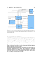
Tau, Trice); others at least partly keep the implementational view, modeling components, e.g., by object communicating by method call (e.g., ARTISAN). This is reflected in the description techniques as well as the operational model supported by the tools.
3.2.1
Available Description Techniques
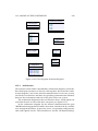
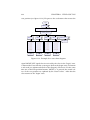
All tools support four common classes of description techniques:
Structural Descriptions describing the architecture of the system consisting of components, interfaces (e.g., ports, sensors, actors), communication paths (e.g, channels, connections). Examples are System Architecture Diagrams in Artisan, or Block Diagrams in ASCET-SD.1
State-Based Descriptions describing the behavior of the system using states,
transitions, actions or events, and timing annotations. Examples are
State Transition Diagrams in AutoF OCUS and Matlab/Simulink (different variants).
Scenario-Based Descriptions describing exemplary execution sequences
consisting of interactions between components or their continuous
data flow (e.g., in an Oscilloscope-like manner). Examples are Sequence Diagrams in Rhapsody in MicroC and Rational Rose RT.
Data Description describing the data types used to define messages, signals, or variables. Examples are Class Diagrams in Telelogic Tau and
Trice.
The first three are generally defined using a graphical description (including complex textual expression, e.g., for the description of transitions or
events/interactions), the latter either graphically or textually.
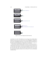
Note that there are two different forms of structural descriptions typically found in embedded systems:
Component Structure: describing concurrently active networks of distributed
components, loosely synchronized by message communication; generally, each component represent a heavy-weight process. Examples
are Architecture Diagrams in Tau, Capsule Diagrams in Rose RT and
Trice, or System Structure Diagrams in AutoF OCUS.
Data Flow: describing units of computation which are activated sequentially, tightly synchronized by the data flow between them; generally,
1
Note that, influenced by the UML, class or object diagrams are partially used to describe
structural aspects; however these are generally enhanced by some form of architecture diagrams.
CHAPTER 3. RESULT SUMMARY
28
each block represents a light-weigh task. Examples are Block Diagrams in ASCET-SD or MATLAB/Simulink.
Furthermore, some tools offer additional description techniques:
Scheduling and Real-Time Aspects: used to describe the task structure of
the system and the schedules of activation (e.g., ASCET-SD, Artisan).
Additional Analysis Descriptions like UML Use Cases, Process or Activity Diagrams, e.g. used to describe the functional structure or the
technical process controlled by the system (Artisan, Rhapsody in MicroC, Rational Rose RT)
Implementation Organization: Package, Deployment, or Component Diagrams, used to describe the code package structure (e.g., Artisan,
Rational Rose RT); Mapping Descriptions, used to described the mapping between interface elements and memory areas (e.g., ASCET-SD,
Artisan).
To structure the specifications, throughout the tools, each (graphical) description technique supports hierarchical structuring (e.g., component/subcomponents, state/sub-states).
3.2.2
Applied Description Techniques
As mentioned above, most tools focus on a small set of description techniques covering structure, behavior, interaction, and data. UML-driven
approaches (e.g., Artisan, Rose RT) add additional description techniques;
some complementary (e.g. Use Case Diagrams), some focusing on implementational aspects (e.g., Package Diagrams or Component Diagrams),
others describing similar or overlapping aspects (e.g., Collaboration Diagrams and Sequence Diagrams). Since in those approaches not always all
notations are applied, this section focuses on the description techniques
applied in the case study.
In general only those description techniques were intensively applied
which are - more or less - directly integrated in the development process
(see also 3.3): either because a simulatable specification or code can be generated from them (like from structural, behavioral, or data descriptions),
or because they are generated from other descriptions (like interaction descriptions). To a limited degree, other description techniques are used to
get a first impression when analyzing the system, like interaction descriptions and Use Cases. Since those description techniques are only weakly
integrated in the development process (e.g., no other descriptions can be
generated from them or checked against them), they are only used sparingly.
3.2. MODELING THE SYSTEM
29
Finally, the case studies are focusing on modeling the system rather
then implementing it. Therefore, the above-mentioned aspects of defining task and schedules as well as organizing the system in packages were
kept to a minimum; accordingly, corresponding description techniques are
hardly used.
In general, the tools focus on the four common description techniques
to specify and validate the system under development. Accordingly, in
the case studies, mainly those description techniques were applied to describe structure and interfaces, behavior, interaction, data. Additionally,
were available, use cases were used in an early stage to structure the functionality and to collect interface information. Since basically, structure, behavior, and data descriptions are sufficient to describe an executable model
of the system, all sets of description techniques offered by the tools were
considered to be sufficient. If no interaction descriptions by event-based
forms like sequence diagrams were available (e.g. Matlab/Simulink), those
were found missing. Furthermore, hierarchy within graphical description
techniques (e.g., state/sub-state) was considered essential in all tools (e.g.,
Telelogic Tau).
The use of graphical description techniques combined with the possibility of abstraction/hierarchical structuring was considered to greatly improve the clearness of the model. Generally, clearness of the model was
interpreted as being related to the simplicity of the model, resulting in
reducing the number of connections between modeling elements (especially, transitions); non-surprisingly, this reduced complexity per view is
achieved at the cost of deeper hierarchies.
3.2.3
Complexity of Description
The complexity of descriptions is influenced by factors like
Hierarchy support reducing the complexity by hierarchically structured
descriptions (e.g., state/sub state) and corresponding mechanisms
(e.g., group transitions for a hierarchical state)
Computational model affecting the resulting complexity of the annotations (e.g., parallel reception of signals vs. accepting only one method
call at a time) as well as the number of transitions
Furthermore, the level of abstraction does of course influence the complexity, e.g. using abstract signals instead of CAN-bus signals.
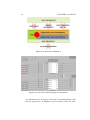
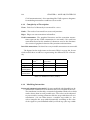
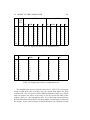
Nevertheless, the complexity of the specifications is more or less within
the same order of magnitude for the tools. Especially, the average complexity per view is similar between most tools (4 nodes, 7 edges); this indicates
suitable modular description techniques supporting readable designs. In
short, the following complexity measures were obtained:
CHAPTER 3. RESULT SUMMARY
30
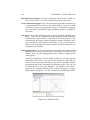
Views: The number of views varies between 14 and 90, with an average
around 40 views used to model the controller.
Nodes: A total number of about 100 nodes average where needed to model
the system.; the average number of nodes per view is about 4.
Edges: The total number of edges used in the specification ranges about
between 150 and 300 edges; the average number of edges per view is
about 7.
Visible annotations: The average length of visible annotations used to
specify the controller is between 30 and 60.
Invisible annotations. While in most tools no invisible annotations where
used, in some tools (e.g., AutoF OCUS) complex annotations (like transition triggers) where hidden and replaced by a short explanatory label.
For some of the tools, the reported figures are outside this range. With
ARTISAN, the statistics were applied to the more abstract design, leading
to a deviation from the mean. Due to its operational model tuned especially toward control algorithms, the MATLAB specification has a slightly
higher complexity for this event-based case study. For Telelogic Tau, the
deviation can be attributed to the more structured representation of state
diagrams similar to SDL. In case of Trice, overlaps in the representation
where counted multiply; otherwise, basically a result close to the statistics
of Rose RT would have been measured.
3.2.4
Operational Model
Obviously, the choice of the operational model used to interpret the diagrams influences the complexity of the description. For instance, an operational model supporting buffered communication can simplify the description of a message handling strategy. Furthermore, it also influences
the expressibility of the modeling language. For instance, a formalism supporting the explicit description of parallel events allows to detect simultaneously occurring events, which is not expressible in a language without
this feature. Therefore, in this section we give a short description of the
operational model underlying the tools.
When describing the behavior of a reactive system, the description of
interactions between its components plays a central role. The interaction is
influenced by two different forms of synchronization:
Message Synchronization: This form describes the coupling of sender and
receiver of a communication. Message-synchronous communication
corresponds to a handshake communication blocking the sender of
3.2. MODELING THE SYSTEM
31
a message until the message is accepted by the receiver. With message
asynchronous communication, the sender of a message is not influenced by the receiver of the message; the receiver will always accept
the message. This is either the case with buffered communication where
the receiver buffers unread message until consumption or with signalbased communication where unread messages are overwritten by new
arriving messages.
Time Synchronization: This form described the synchronization of the
actions of different components. In event-driven systems, behavior is
triggered by the occurrence of events; in time-driven systems, behavior is triggered by the passing of time.2
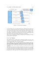
The applied tools use different combinations of those synchronization aspects:
Artisan: Method-based, event-driven: Artisan uses a method-based communication model. The exact interpretation of the method call (message-asynchronous or message-synchronous) is left open and depends
on the implementation platform. Since objects are activated by communication events, the model operates in an event-based fashion.
ASCET-SD: Signal-based, time-driven ASCET-SD uses a signal-based communication. Time synchronization usually is performed time-driven
with individual rates for the components; additionally, there are some
predefined events like interrupts.
AutoF OCUS: Signal-based, time-synchronized event-driven: AutoF OCUS
uses a signal-based communication. Concerning time-synchronization
it uses a hybrid model. Communication is performed in a synchronized manner: all components communicate in a time-driven roundbased scheme with a global time-rate for all components. Within
each round events for occurrence of a message as well as as the nonoccurrence can be detected.
Matlab/Stateflow: Signal-based, time-driven Matlab/Simulink use a signal-based communication. Time synchronization usually is performed
time-driven with individual rates for the components; additionally,
there are some predefined events like function calls, or value changes
(rising/falling edges).
2
Note that from a formal point of view event-driven systems can be transformed into
time-driven system and vice-versa, either by adding timing events or by adding explicit
absence events; however when considering additional restrictions like idle-load or efficient
simulation, those transformations are not always suitable.
32
CHAPTER 3. RESULT SUMMARY
Rhapsody: Signal-based, time-synchronized event-driven: Rhapsody in
MicroC uses signal-based communication. Concerning time-synchronization it uses an hybrid model. Communication is performed in a
synchronized manner: all components communicate in a time-driven
round-based scheme with a global time-rate for all components. During each round boolean events and change events are created in a ‘run
to completion’ form (till no more transition can be fired).
Rose RT: Buffered, event-driven : Rose RT uses a buffered communication
model, additionally supporting an explicit wait for a return value.
Components get activated whenever messages are available; if a component is not ready to accept messages from sending components,
those messages are stored in a message queue in the order of arrival.
Tau: Buffered, event-driven: Telelogic Tau uses a buffered communication model. Components get activated whenever messages are available; if a component is not ready to accept messages from sending
components, those messages are stored in a message queue in the order of arrival. Timers are used to generate time-out messages.
Trice: Buffered, time-driven: Trice uses a buffered communication model.
Similar to AutoF OCUS, during a cycle of the system each component
executes a step if a transition is enabled. Additionally, timers can be
used to generate timeout messages. If a component is not ready to accept messages from sending components, those messages are stored
in a message queue in the order of arrival.
Generally, all operational models have been found sufficient by the users
of the tools. However, extensions of the models with simple properties can
sometimes reduce the ease of handling. Examples are:
Signal-buffering: In signal-based communication, explicit buffering of messages can reduce the complexity of the model in situations with weak
synchronization of the models.
Channel-based communication: For channel-based systems relying on 1:1
communication, a multi-cast mechanism can reduce unnecessary connectivity.
Concerning support for the real-time aspects of embedded systems,
there are different possible approaches:
Timed model: The operational model explicitly deals with time. Depending on the synchronization mechanism of the model, there are different variants: event driven models generally use some form of timeout
event triggering behavior; time-driven models usually have a scheduled execution model supporting access to some system clock variable.
3.3. DEVELOPMENT PROCESS
33
Timed deployment: The operational model does not directly deal with
time. At most, timing conditions can be added as annotations.
Different timing models are used in the tools:
ARTiSAN: ARiTSAN delegates the real-time aspects to the implementation and deployment phase.
ASCET-SD: ASCET-SD uses a time-driven model (with individual frequencies, based on the operating system) with a variable indicating
the time difference to the last execution time.
AutoF OCUS: AutoF OCUS uses a time-driven model with a universal clock;
timers can be introduced based on the global clock tick.
MATLAB/StateFlow: MATLAB/StateFlow uses a time-driven model (with
individual frequencies, based on the operating system) with a variable indicating the system time as well as special time event.
Rose RealTime: Roses uses timeout-events generated from a timing service to support time in its event-based model.
Rhapsody in MicroC: Rhapsody uses timeout events as well as scheduled
actions to add event-driven time support. The actual timing behavior (including the frequencies of its time-driven behavior) is added
during deployment.
Telelogic Tau: Tau uses timeout-events generated from timers specific to
a component to support time in its event-based model.
Trice : Trice delegates the real-time aspects to the implementation and deployment phase.
Independent of the timing model, to meet real-time bounds, during deployment schedules and frequencies depending on the hardware platform
have to be defined or connections to the real-time features of the operating
systems must be established. Finally, depending on the parallelism available in the operational model, explicit tasks and interrupt levels must be
defined. Both aspects are not treated here.
3.3
Development Process
While the previous section focuses on the properties of the model of a system, this section rather addresses the question how such a model is built.
Since – as argued in Chapter 4 – a major advantage of a model-based development process lies in the analysis and construction support on the level of
the abstract model, Subsection 3.3.2 takes a close look at that subject.
CHAPTER 3. RESULT SUMMARY
34
3.3.1
Applied Process
Obviously, the applied process is defined by the description techniques and
process support supplied by the used tools. Nonetheless, a common development process independent from the tools can be established. Generally,
in each tool application the applied process was constructed by leaving out
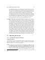
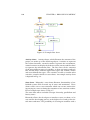
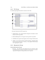
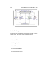
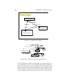
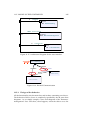
phases or activities of this general process. This overall applied development process consists of three main phases:
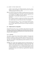
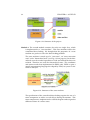
Analysis: The purpose of this phase is to get a better understanding of
the system and to identify groups of functionality (controlling the
seat, controlling the locking of the door, and the overall user management). Due to restriction of notations, this phase is more explicit in
tools supporting additional analysis description techniques like UML
use cases. Nevertheless, in all tools Step 2 was performed:
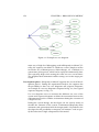
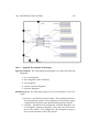
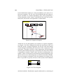
1. Coarsely structuring the functionality of the system, using use
case-like diagrams
2. Defining the system boundary (e.g., actors, sensors, busses), using structural diagrams
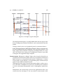
3. Exemplarily defining the functionality of the system using scenariobased diagrams
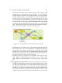
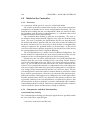
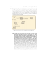
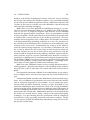
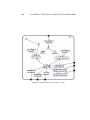
Design: During this phase, the system was generally partitioned to support concurrent engineering and modular development. Note that
this partitioning is performed on structural decomposition (based on
parallelly computing components, generally components to controlling the seat, the locking of the door, and the user management), but
based on the functional structuring identified in the Analysis phase.
These steps were generally explicitly performed in all tool applications:
1. Defining and refining the system structure by introducing (sub)components, using structural diagrams
2. Adding behavior to the (sub-)components, using state-based diagrams or data-flow diagrams
3. Validating and refining the behavior of (sub-)components, using
simulation
Integration/Validation: In this phase, the different components were integrated into one system (generally, due to the component model supported by the tools this requires no additional steps) and validated by
simulation. Generally, Step 1 step was performed by all tool applications:
3.3. DEVELOPMENT PROCESS
35
1. Generating simulations of the complete system, either generating scenario-based descriptions of simulation runs or using simulation interfaces
2. Comparing the simulation results with the scenario-based descriptions
Several of these steps are more explicit in certain processes, depending on
the available and applied process support as explained in the following
Subsection.
3.3.2
Applied Process Support
Development Operations
Simple development operations (e.g., cut-and-past of elements within one
diagram) are generally supported by all tools. Depending on the status of
the tool (academic prototype vs. wide-spread product, new release vs. established product), the stability and functionality of those operations differ.
Complex development operations (i.e. supporting complex stereotypic
or application domain specific operations) generally focus on the support
of the implementation. Typical examples are the generation of schedules
for computations (e.g., ASCET-SD, ROSE RT, Tau) or optimizations for certain platforms. Depending on how strong a tool supports the implementation phase, some of these functionalities may not be available if the tool
focuses on analysis and design (e.g., ARTiSAN). Generally, however, most
of the tools only have restricted complex development support for the analysis or design phase (see also Subsection 3.3.2).
For obvious reasons, reverse engineering (i.e. generating specifications
out of code) can only be partially supported by tools. Generally it focuses
on the structural parts of a system (e.g., generation of class diagrams) or is
limited to code generated by the tool and hardly modified.
Consistency ensurance mechanisms
When building a large specification broken up into several modules or diagrams, frequently errors arise at the interfaces between those parts. Additionally, specification errors also arise within each module or diagram
when parts of these specifications are missing or to not fit together. CASEtool can help to detect those inconsistencies to make the specification consistent. Model consistency can be supported at different levels:
Code Level: On this level, the tool does not directly support model consistency. Rather, syntactic consistency is only defined on the level of
the generated code; generally, the tool however can related code-level
36
CHAPTER 3. RESULT SUMMARY
errors back to the model, e.g., by relating a compiler error to the relevant element of the model.
Syntactic Diagram Level: On this level, the tool makes sure that a single diagram (or view) is well-formed. This is the most basic form of
model consistency. Examples are:
• Well-formedness of trigger expression
• Well-typedness of communication paths (channels and ports have
the same type)
Syntactic Model Level: On this level, the tool ensures syntactic consistency between diagrams referencing the same elements of the model.
Examples are:
• Definedness of types (e.g., types used for messages or variables
are defined)
• Definedness of messages (e.g., messages used in an interaction
description/Sequence Diagram are defined according to the type
of the channel as defined in the structural description/Architecture
Diagram)
Semantic Diagram Level: On this level, the tool ensures well-definedness
of a single diagram, usually requiring some form of execution or verification. Examples are:
• Non-determinism of behavioral descriptions (e.g., no two transitions from one state can be enabled by the same triggering
evens)
• Completeness of behavioral description (e.g., for each possible
triggering event there is an associated transition)
Semantic Model level: On this level, the tool ensures that the dynamic
aspects of the description are consistent - generally, this requires some
form of (symbolic) execution or verification. Examples are:
• Consistency between a behavioral description and an interaction description (e.g., between State Diagram and Sequence Diagram)
• Consistency between interaction descriptions (e.g., between several Sequence Diagrams)
Syntactic diagram level consistency can either ensured constructively or by
analysis. Examples of the first form include editors accepting only structurally well-formed diagrams (all tools), editors accepting only well-formed
trigger conditions (e.g., Rhapsody), or structural editors supporting only
3.3. DEVELOPMENT PROCESS
37
the construction of a connecting channel between ports of corresponding
types (e.g., Simulink/StateFlow). Examples of the second from include editors checking well-formedness of trigger conditions (e.g., AutoF OCUS), or
checking the well-typedness of channels (e.g., Tau).
Syntactic model level consistency, too, can either be ensured constructively or by analysis. The first form is often realized using a common (syntactic) model for all views, e.g., in form of a repository; the constructive
approach includes using only defined messages for channel in a Sequence
Diagram (e.g., Rose RT). The corresponding analytical approach uses an
additional check to ensure this property (e.g., Tau).
Semantic diagram consistency is generally not supported by tools. Few
exceptions exist„ e.g., the non-determinism check (AutoF OCUS).
Finally, semantic model consistency in most tools only support a constructive approach. Generally, this is limited to the construction of scenariobased interaction descriptions, e.g., in form of sequence diagrams; this is
supported by most tools. Few tools support the verification of such an
interaction description against the state-based behavioral description, e.g.
by checking whether a sequence diagram can be executed by the statemachines of the corresponding components; this is, e.g., supported by Rhapsody or AutoF OCUS. General verification techniques (e.g., model-checking)
are generally supported only by academic tools (AutoF OCUS) or by additional linked academic tools(e.g., for StateMate).
3.3.3
Applied Quality Management
The tools show only slight differences in their support for quality management. These can mostly be traced to different basic functionality of the
respective tools. For example, whenever target code is generated, there is
usually also some support for target simulation.
Host Simulation Support. Simulation of the model is generally offered by
the tools. The tools differ as to which kinds of displays are available,
which parameters can be modified, and how flexibly the tool reacts
to changes during simulation.
In some tools, such as Artisan and Rhapsody, display panels are mostly
thought to animate the models, no numeric simulation is available.
Tracing of states visited by a state machine or oscilloscopes for displaying curves are common visualization techniques in simulation.
Target Simulation Support. Some tools do not generate target code, so no
target code simulation is offered. Even if direct target simulation facilities are not provided, as in Autofocus, the generated target code
can in principle be simulated on the target hardware using tools of
third-party vendors.
38
CHAPTER 3. RESULT SUMMARY
Usually, target simulation is subject to some restrictions: Whereas
code can be executed on the target platform and data can be transferred back to the host for display, it is often not possible to interrupt
the simulation process or modify data interactively.
Adequacy. The simulation mechanisms were generally perceived as adequate. Whenever data can be measured, they can also be displayed in
an appropriate graphical form (e.g. curves or dials instead of tables).
Only some of the tools allow parameter adjustment during simulation. It should be noted that our case study did not require complex
parameter fitting, so not all of the tools’ capabilities were exploited.
Debugging Features. In most tools, debugging is synonymous for running a simulation, modifying parameters and observing the outcome.
Technically, simulation is often realized by executing the generated
code which has been especially instrumented (and not just by symbolically executing the model). This gives a high degree of confidence that bugs can effectively be tracked down in the generated
code. Some tools (ASCET, Rational Rose RT, Matlab/Stateflow) offer
the possibility to set watchdogs for certain variables or events. Beyond that, only Matlab seems to provide a more elaborate code level
debugger.
Testing. Almost all tools allow parameter vectors to be played back during a simulation, and current simulation data to be saved for later
use, for example in regression testing. Apart from that, there is little
support for test data management, like batch processing of test suites
and generation of test statistics. Test coverage analysis is provided by
Rational Rose RT (interface to an external tool) and Matlab. However,
automatic generation of test cases out of the model does not seem to
be offered by any of the tools.
Certification Most of the tools are not certified. Trice has started a TÜV
certification. Parts of ASCET have been TÜV certified; the exact extent of this certification is not clear.
Requirements tracing None of the tools directly integrates requirements
tracing. However, several tools offer an interface to external requirements tracing facilities, such as Doors.
The above remarks can be summarized by saying that the most important quality assurance method is simulation. The tools are generally very
well developed in this area. However, “debugging” and “testing” are just
understood as variations of simulation. Genuine support for testing (automatic derivation of test cases; test analysis including test coverage metrics)
3.3. DEVELOPMENT PROCESS
39
is not provided by the majority of tools, static analysis techniques are missing almost entirely (also see Section 3.3.2). Since all these quality assurance
mechanisms are required in standards like IEC 61508, it is not surprising
that only very few tools have been certified so far.
3.3.4
Applied Target Platform
Since code was not deployed in this case study, this section gives only a
short overview about tool features for target code generation and deployment.
Target code generation and supported targets. All of the reviewed tools
support the generation of code that can in principle be run both on
the host and the development target. The C and C++ languages are
supported by all tools; in addition, Rational Rose RT supports Java
code generation. Usually, running the code on a target would require
adaptations like adaption to the language subset supported by the
target compiler or appropriate operating system calls and configuration. As a notable exception, ASCET-SD, Matlab/Simulink, and Trice
support a range of embedded targets and rapid prototyping environments by compiler and OS-specific adaptations of the generated code.
Code size. The target code size (binaries) tended to be in the 8-80kByte
range, while memory consumption was up to 800kByte for the running model on the host. These figures are preliminary results, as the
focus of the evaluation was not on code generation.
Readability of code. Readability was found to be good for all of the evaluated tools. All of the tools use identifiers from the model in the code;
if state machines are implemented, the structure is generally replicated in the code’s control structure. Comments from the models are
usually included in the source files.
3.3.5
Incremental Development
Reuse, restricted changes, and modular design. Support for reusability and
the restriction of changes to localized parts of the model were generally found to be adequate. All of the evaluated tools supported some
notion of a reusable component or actor, thus simplifying architectural changes and reuse of existing components. As the only research
tool in the comparison, AutoF OCUS was found to lack support for
bottom-up structuring. Moving from the first iteration to the second,
changes in the specification were found to be restricted to some components, not affecting the specification as a whole. Reuse of partial
CHAPTER 3. RESULT SUMMARY
40
specifications was typically performed by simple copy/paste mechanisms; library mechanisms as in Matlab/Simulink and AutoF OCUS
have also proven to be helpful.
Restructuring. As of now, most of the tested tools lack automated support
for restructuring and refactoring. As a notable exception, the two
UML-RT tools, Rose RT and Trice, offer automated composition and
decomposition of actors (“aggregate function”).
3.4
Conclusion
Table 3.1 gives a summary of the perceived strengths and weaknesses of
the tools.
Obviously these perceived strengths and weaknesses do not always correspond with the strengths and weaknesses experienced by expert engineers. Therefore, features like support for platform-tailored code-generation
(e.g., Rhapsody in MicroC, Trice), in-the-loop tests or test case-generation
(e.g., ASCET-SD, Telelogic Tau), connection to project-support tools (e.g.,
Rose RT, ARTiSAN), transformations like discretization (e.g., MATLAB/
Stateflow), or verification (e.g., AutoF OCUS) were perceived as important
issues. Nevertheless, these perceived strengths and weaknesses have a decisive influence on the long-term adoption of a tool.
As a conclusion, all of the groups managed to design fully functional
models of the case study in their respective tools. The evaluated tools have
shown a good balance of user support and usability, support for quality
control, and target code generation. As the only research tool in the comparison, AutoF OCUS naturally showed some weaknesses regarding user
friendliness, documentation, and stability, while otherwise holding up well
against the commercial tools. MATLAB/Stateflow, ASCET-SD, Rhapsody,
and Trice, being somewhat more targeted at small embedded targets, have
strong support for target code generation. The tools from the classical
SW engineering or telecommunications domain, ARTiSAN, Rose RealTime,
and Telelogic Tau, excelled in terms of usability and user support. A common weakness of all of the above tools seems to be the almost nonexistent
support for automated or semi-automated development steps like restructuring and refactoring.
3.4. CONCLUSION
Tool
ARTiSAN
ASCET-SD
AutoF OCUS
MATLAB/StateFlow
Rhapsody in MicroC
Rose RealTime
Telelogic Tau
Trice
41
Strengths
Good overall usability
Tight consistency check
Good support for modular descriptions
Wide variety of notations
Strong target code generation
Good support for modular descriptions
Good
simulation/validation
support
Good readability of
generated code
Good usability
Good modeling notation
(Limited) support for
reverse
engineering
code
Good modeling notation
Useful simulation and
debugging
environment
Good interoperability
with 3rd party tools
Good usability
Fully constructive behavioral model
Good usability
Strong target code generation
Weaknesses
No explicit target code
generation
Usability could be
improved
Loose
consistency
check
No integration with
version management
Weak usability
Editor runs instable
Consistency
checks
need improvement
Insufficient
namespace concept
No sequence diagrams
Built-in
database
causes
versioning
problems
Limited
support
copy/paste
SDL-style notation may
be unfamiliar to UML
developers
Documentation incomplete
Table 3.1: Strengths and Weaknesses of the CASE tools
42
CHAPTER 3. RESULT SUMMARY
Chapter 4
Model-Based Development:
Executive Summary and
Picture of the Future
Bernhard Schätz
When looking for a definition of what model-based software development is (or is not), there is a wide range of different interpretations. However, most approaches have in common:
• the use of graphical representations for the system under development
• the possibility to describe the system (or software) with a certain degree of abstraction from the actual implementation platform
• the possibility to generate an executable system out of the model
As shown in Chapter 3 and in more detail in the chapters of the second part,
current CASE tools for embedded systems do support those functionalities;
additionally, those tools generally offer support
• to describe the system using different views (at least: data, structural,
state-based/behavioral, scenario-based)
• to hierarchically structure views
• to use message- or signal-based communication in the operational
model
• to include timing aspects in the description of the system
• to check the model for inconsistencies, mainly on the syntactic level
(e.g., undefined identifiers, type mismatches)
43
44
CHAPTER 4. MODEL-BASED DEVELOPMENT
• to simulate the system (or software) at the level of the description
Implicitly or explicitly, most model-based approaches aim at increasing
both
• the efficiency of the development process (by increasing the degree of
mechanization), and
• the quality of the development product (by decreasing the amount of
possible errors).
In order to achieves these goals, however, support for a model-based development for embedded systems should exceed
Using an implementation-level model: Modeling the system at code level
rather than at a more abstract level leads to a limited development
process, focusing on the implementation and integration phase. Thus,
e.g., defect analysis is limited to implementation level defects. This
excludes simple defects like message interface incompatibility between
processes executed on different nodes since those messages are described as a byte-block oriented bus-protocol. Furthermore, due to
the gap between the earlier phases and the implementation level,
even design specifications are not always related to the implementation. This is often leading to inconsistencies between the design and
the implementation.
Using an OO-model for embedded software: OO-based approaches supply different views of the system including non-executable views for
early phases (e.g., use case description, interaction scenarios) making
consistency analysis available in those phases. However, those views
offer only limited abstraction from the OO operational model; e.g.,
(synchronous) method calls are used to model interaction between
tasks rather than the more suitable message- or signal-based communication. Furthermore, additional domain-specific aspects (e.g., bus
schedules, task switching) are not modeled explicitly. Therefore - to
obtain deployable code - those aspects are laid off to the coding phase
outside the modeling capability of the tool, leading to similar problems as with implementation-level models
Using a Draw-and-Generate Tool: Domain-specific approaches generally
support a more detailed model including aspects like preemption or
time-driven communication allocatable to bus slots; these tools make
use of this information to generate deployable code. However, generally sophisticated analysis techniques are not available on the level of
the model; therefore, the analysis of defects introduced on the level of
the model is performed manually or is delayed until the execution of
45
the generated model. Thus, e.g., the consistency between time-driven
communication and allocated bus schedules is not ensured.
Using a loosely coupled tool chain: A loosely coupled tool chain generally splits the development process in tool-related phases with substantial gaps between those phases; often a high degree of integration is missing. Examples for those gaps in the development process are scenario-based descriptions of the behavior that cannot be
used to generate equivalent test cases on the implementation level,
or counter-examples generated by verification or validation on the
level of implementation which are not expressed on the level of the
abstract system. Therefore, the tool chain depends heavily on those
forward and backward integrations and a common model bridging
the tool chain. Since those steps are limited by the information explicitly represented in model of each tool of the chain, the degree of
coupling is limited by the quality of those models and their interdependence. If, e.g., the bus signal communicated on the implementation level cannot be related back to messages communicated between
abstract components, counter-examples cannot be expressed on that
abstract level.
The construction of reliable (embedded) software is of course possible without a model-based development process. However, research results suggest that such a process can contribute essentially to increase the quality of
the developed product as well as to an increased efficiency of the development itself:
• [Jon91] shows that more than 50 % of serious errors are made during
design (25 % during implementation); about 30 % of medium errors
are made during design (30 % during implementation)
• [Jon91] shows that analytical techniques performed on early-phase
description of the product (e.g., structured approaches, design reviews) require generally at least less than 50 % of the effort in both
error detection and correction needed for later-phase techniques (e.g.,
integration test, field test)
• [Jon91] shows that those analytical techniques of the early phases are
at least twice as effective to detect errors of the early phases than those
later-phase techniques.
• [BMJH96] shows that especially in a development process requiring a
high level of product quality, CASE support can significantly increase
productivity.1
1
Productivity is measured in implemented function points per time unit.
46
CHAPTER 4. MODEL-BASED DEVELOPMENT
In our understanding (see also [SPHP02]), a model-based software development process requires
• a product model integrating different views of the system for different stages of development and different levels of abstractions
• a CASE-supported development process offering techniques to analyze the product model on all levels of abstraction and supporting
transitions between those levels.
These properties have immediate consequences on how a tool should support a model-based development process: it concerns what aspects or views
of the system under development should be covered by the tool as well as
what kind of operations should be offered by the tool to analyze or transform the model:
Adequate Models: During the development process, different aspects of
the system under development must be addressed (for the domain
of embedded systems, e.g., overall functionality, time and resource
limitation, partitioning and deployment, scheduling) during different
phases (e.g., requirements analysis, design, implementation, integration). Specific views must be available for these phases. Since software systems, and especially embedded software systems, are moving from monolithic single-functionality programs to distributed, interactive multi-functionality networks, a central aspect of such a model
is treatment of interaction and communication as well as time-related
aspects. Furthermore, a model must support specific aspects needed
for the application domain (for the domain of embedded real-time systems, e.g., notions like messages or signals, task, schedule, controller,
bus). By supporting domain- and application specific modeling elements, more information about the system under development is
represented in the model, leading to stronger analysis and generation techniques (e.g, in the domain of embedded systems, checking
the wort case time bounds of a task, or generating a bus schedule
from the communication description of a component model).
Abstract Models: A model should contain only those aspects needed to
support the development phase they are applied for (e.g., modeling
the interaction between components by messages rather then method
calls to the bus driver or the operating system). By abstraction a
model reduce the complexity of description as much as possible as well
as the possibility to produce faulty descriptions (e.g., ensuring type correctness between communication ports rather than using byte block
messages on the level of bus communication). Furthermore, an abstract model also supports descriptions of the system under development in early analysis and design phases, making analysis and gen-
BIBLIOGRAPHY
47
eration support available even at early stages of the development process (e.g. completion of state-based description of a component to
introduce standard behavior for undefined situations).
Integration by Analysis: The relation between different models during
the development is supported. This includes the analysis of different
models used during the same phase (e.g., checking the consistency
of a exemplary sequence diagram and a complete state-transition description of a component) as well as different phases (e.g., checking
a bus communication schedule against the abstract communication
behavior of the corresponding abstract component). This leads to a
higher level of product quality, especially by supporting analysis of
the system at earlier stages; furthermore it also increases process efficiency by supporting earlier detection of defects.
Integration by Generation: The transition between different views or version of a model in the development process is supported by generating views or versions of the model out of each other. This includes
forward generation (i.e., from a view of an earlier phase to the view
of a latter phase; e.g., the generation of test cases from a behavioral
description) as well as backward generation (i.e., from an implementation view to a more abstract one; e.g., the generation of an abstract
scenario-based description from an execution trace of the implementation level). This leads to increased process efficiency by a higher
degree of automation as well as increased product quality by eliminating defects introduced by manual development steps.
Recent analysis suggests that currently available CASE support does indeed lead to a significant increase in productivity. However, especially
in the field of automotive industry, the increase of system complexity has
grown faster than the increase in productivity for the last 10 years. As argued above, model-based development promises to help closing this gap
by shifting analytical and generative techniques from the level of implementation to the level to specification and modeling. Current research (e.g.,
[PLP03], [SBHW03]) shows that model-based tool support is technically
feasible.
Bibliography
[BMJH96] Tilmann Bruckhaus, Nazim Madhavji, Ingrid Janssen, and John
Henshaw. The Impact of Tools on Software Productivity. IEEE
Software, 13(5):29–38, 1996.
[Jon91]
Capers Jones. Applied Software Measurement. Software Engineering Series. MacGraw Hill, 1991.
48
[PLP03]
CHAPTER 4. MODEL-BASED DEVELOPMENT
Alexander Pretschner, Heiko Lötzbeyer, and Jan Philipps.
Model Based Testing in Incremental System Development. Journal of Systems and Software, 2003.
[SBHW03] Bernhard Schätz, Peter Braun, Franz Huber, and Alexander
Wisspeintner. Consistency in Model-Based Development. In
Proceedings of ECBS 2003 10th IEEE International Conference. IEEE
Computer Socienty, 2003.
[SPHP02] Bernhard Schätz, Alexander Pretschner, Franz Huber, and
Jan Philipps. Model-based Development of Embedded Systems. Technical Report TUMI-0402, Fakultät für Informatik, TU
München, 2002.
Part II
The Tools
49
Chapter 5
Tool ARTiSAN RealTime
Studio
Christoph Angerer, Martin Glaser and Christian Merenda
5.1
General Aspects
ARTiSAN RT Studio is a development platform for embedded systems. It
is mainly based upon the UML 1.4 (Unified Modeling Language) extended
by some enhanced notation techniques. This paper evaluates capabilities
as well as possible weaknesses of ARTiSAN RT Studio. Basis for this evaluation was a shortended version of the case study “Das Türsteuergerät eine Beispielspezifikation”, which can be found at
http://www.iese.fhg.de/pdf_files/iese-002_02.pdf.
• Section 1 gives a short overview over ARTiSAN RT Studio
• Section 2 describes the features of ARTiSAN RT Studio for modelling
systems as well as as which features we used, including some experiences, during the case study.
• Section 3 deals with the subject development process, especially how
ARTiSAN RT Studio supports managing development.
• Finally, after a conclusion in Section 4, we introduce our model of the
door controller in section 5.
5.1.1
Functionalities
ARTiSAN RT Studio supports several modeling diagrams. The standard
UML diagrams (these are: Activity Diagram, Class Diagram, Object Col51
52
CHAPTER 5. TOOL ARTISAN REALTIME STUDIO
laboration Diagram, Object Sequence Diagram, State Diagram, Use Case
Diagram) and some enhanced diagram types (these are: Concurrency Diagram, Constraints Diagram, System Architecture Diagram, Table Relationships Diagram, General Graphics Diagram, Text Diagram). Out of the developed model, "Code Generators" for Java, C++, C and Ada undertake the
tasks of generating code skeletons.
Furthermore ARTiSAN RT Studio offers two simulation techniques for
validating the models: With "Object Animator" the interactions within the
modeled object sequence diagrams can be visualized and the "State Machine Generator" generates code to simulate the behaviour of the system.
An extension called "Altia Faceplate" in combination with the State Machine Generator can even be used to create simple demo applications.
The "Document Generator" is responsible for the documentation process. The result is a Microsoft Word document, which can be edited further
on. It contains the details of the different diagrams.
Configuration management is based on a central database, where all
models are interconnected with one another. So it is possible to work in a
team, without running into the failure of inconsistency. Each code generator includes the funtionality to synchronize code with a model to keep the
source code and model in step.
Test management and test case generation is described at length, but
there´s no direct support for these activities.
During every phase of the development process, the model can be automatically verified. With the "Report/Consistency" function, leaks within
the model can be discovered. Even though the models are implicetely consistent because of the underlying database, apparent design failures are
reported. Unfortunately, not all information of the model is used for this.
For example, wrong parameter passing between objects in a sequence diagramm is not recognized.
5.1.2
Development phases
ARTiSAN RT Studio assists the developer during the two phases requirements analysis and design (= modeling). The implementation activity is confined to code generation (class skeletons) and the synchronization functionality between code and model. Test and deployment is not supported. All
development phases are vividly described in the so called RtP mentor (see
5.1).
5.1.3
Documentation
There´s no print version of the manual available. The online help is very
good, not only because of the clearly arranged information and graphical
5.2. MODELING THE SYSTEM
53
representation in the RtP mentor, but also the extensive information behind
the scope of the provided functionality is very useful.
5.1.4
Usability
All in all the usability of ARTiSAN RT Studio is good. The handling is very
intuitive. The main issue the authors have to mention are the long waiting
periods, e.g. during the import/export of models in the so called models neighborhood or the copy/paste operation between different diagrams.
Besides the team wants to point out some minor aspects:
• The user only has weak control over the presentation of model elements (e.g. shadows, line thickness)
• some graphical elements cannot be resized and
• after copy/paste operations all objects (interface devices, classes, etc.)
are arranged one upon the other.
5.2
Modeling the system
This section describes how ARTiSAN RT Studio supports modeling a system and which features were used to model the case study.
5.2.1
Available Description Techniques
ARTiSAN RT Studio offers several diagram types. Each diagram type can
be used to express different views on the model. This section describes,
which diagrams are offered, what they can be used for and which graphical
elements provide their functionality.
Supported notations
The different diagram types supported by ARTiSAN RT STUDIO are listed
here. According to figure 5.1 they are grouped by the scope and the model
they get used.
54
CHAPTER 5. TOOL ARTISAN REALTIME STUDIO
Figure 5.1: Models supported by ARTiSAN RT Studio
5.2. MODELING THE SYSTEM
Scope
Requirements
Solution
Model
System Scope Model
System Usage Model
System Modes Model
System
Constraints
Model
Dynamic Model
Interaction Model
Class Model
Concurrency Model
Persistence Model
System Architecture
Model
General
55
Diagram types
System Architecture Diagram
Use Case Diagram, Sequence
Diagram
State Diagram
System Constraints Diagram,
Use Case Diagram
State Diagram, Activity Diagram
Sequence Diagram, Object
Collaboration Diagram
Class Diagram
Concurrency Diagram
Table Relationships Diagram
System Architecture Diagram
General Graphics Diagram,
Text Diagram
Modeling aspects
ARTiSAN RT Studio supports the development process exactly as described
in the RtP Mentor. According to this sample process, System Architecture,
Use Case, Constraints and State Diagrams are first used to express system
requirements. Out of this analysis, an Object Architecture emerges using
Class, State and Object Collaboration Diagrams. For the Software Architecture the diagram types Class and Concurrency get used. At last the solution
system is modeled again with the System Architecture Diagram.
In the following, a survey of the usage of the different diagram types
as suggested by ARTiSAN is given. Additionally, all possible graphical
elements for each diagram are listed.
A System Architecture Diagram, an ARTiSAN RT Studio extension to the
UML, declares the software boundary with usage scenarios depicted as
events flowing between Subsystems, Actors and Interface Devices. In fact,
it describes the system structure.
Elements used
Interface Device, Multidrop Bus, Subsystem, Actor, Link,
Event Message
unused Disk, Board
56
CHAPTER 5. TOOL ARTISAN REALTIME STUDIO
For describing the static system structure the Class Diagram is designated.
Elements used
Class, Attribute, Operation, Generalization, Aggregation,
Association, Uni directional association, Dependency
unused Package, Association class link, Ternary Association, External Class
The Use Case Diagrams details the ways in which a designed system can be
used
Elements used
Actor, Use Case, Interaction, Extend Flow, Include Flow,
unused Generalization
Key Use Cases can be explored by modeling a Sequence Diagram, which
shows the system interaction.
Elements used
Sequence, Selection, Outcome, Iteration, Parallel, Also Parallel, Actor, Interface Device, Subsystem, Package, Class,
Timing Constraints, Operation, Event, Include Probe, Extend Probe
unused External Class
The behaviour and the aspects of a system concerned with time and the
sequencing of operations will be defined in the State Diagrams.
Elements used
Initial State, Final State, Atomic State, Transition, Event Action Block
unused History State, Junction State, Sync State, Concurrent Compartment, Synchronization, Sequential State, Concurrent
State, Activity
An Activity Model Diagram can be used to design the dynamic aspects of a
system.
Elements used
Diagramtype not used
unused Action Object, Action State, Sync Bar, Decision Connector,
Initial State, Final State, Signal Send, signal Receive, Control
Flow, Object Flow
The dynamic behaviour can be also described a Object Collaboration Diagram
and so these type of diagram explains a usage scenario.
Elements used
Diagramtype not used
unused Actor, Class, External Class, Link, Operation Message, Event
Message
5.2. MODELING THE SYSTEM
57
A Constraints Diagram is an ARTiSAN RT Studio extension to the UML used
for modeling constraints applicable to real-time systems.
Elements used
Consrtaints Type, Constraint, Link
unused
Concurrency Model Diagrams are an ARTiSAN extension to the UML that
describes the multitasking and concurrency processes that allow a system
to execute within defined performance constraints. asdfsadf
Elements used
Diagramtype not used
unused Class, external Class, Interface Device, Task, Channel, Event
Flag, Mailbox, Monitore, Pool, Semaphore, Signal, Link,
Event Message, Operation Message
Table Relationships Diagrams are used for modeling persistent data storage.
Elements used
Diagramtype not used
unused Table, Column, One-to-many relationship, One-to-one relationship
A General Graphics Diagram is an additional diagram type for modeling various scenarious.
Elements used
Diagramtype not used
unused General Flow, Box, Softbox, Circle, Ellipse, Parallel, Diamond, Component, Node, Small circle
Type of notations
Almost all diagrams are graphical with additional text elements. An exception is of course the Text Diagram.
Hierarchy
It is possible to interlink various diagrams and to create sub-diagrams for
single elements of a model. The interconnection between the diagrams can
be hierarchically structured.
5.2.2
Applied Description Techniques
During modeling the case study, some, but by far not all, features of ARTiSAN RT Studio had been used. Used notations, unused notations as well
as some experiences are described in this section. Detailled informations
about used and unused diagram elements are shown in section 5.2.1.
CHAPTER 5. TOOL ARTISAN REALTIME STUDIO
58
Applied notations
The diagrams we used for modeling our system were:
• System Architecture Diagram
• Use Case Diagram
• Class Diagram
• Sequence Diagram
• Constraints Diagram
• State Diagram
Modeled aspects
According to the offered modeling aspects we have designed the interfaces
on a System Architecture diagram. The behavior and interaction were designed in several State and Sequence Diagrams based on a Use Case Diagram. In one Class Diagram the structure of the system is shown.
Notations suitable
The used notations are suitable for modeling the system.
Clearness
The diagrams consist of self-explaining graphical elements so the meaning
can be understood quickly. According to the UML specification only a few
different elements can be inserted into every diagram type. The graphical
representation of the model is clear and straightforward, because details
are kept separated in a property window.
Unused notations
We have not used some of the offered notations. These were:
• Activity Diagram
• Concurrency Diagram
• Object Collaboration Diagram
• Table Relationships Diagram
• General Graphics Diagram
5.2. MODELING THE SYSTEM
59
• Text Diagram
We were able to model the whole system with the applied notations. Additional diagrams would have contained redundant informations or were
not necessary for our purpose.
Missing notations
We have not missed any notations.
5.2.3
Complexity of description
In this part we only consider diagrams which are used for executing/simulating
the model. These are the state and class diagrams.
Views
Five state diagrams and one class diagram were used.
Nodes
State diagrams
Class diagram
In all there are 24 nodes. The maximum per view is eight,
average is five.
13 nodes
Edges
State Diagrams
Class diagram
50 Edges were used. The maximum is 18, average is ten
16 edges
Visible annotation
State diagrams
Class diagram
152 annotations are visible, maximum is 56, average is 30.
51 visible annotations
Invisible annotations
State diagrams
Class diagram
5.2.4
There are no invisible annotations.
no invisible annotations
Modeling Interaction
An important task during the development process is to model the interaction between system components and objects. This section shows, how this
task is implemented by ARTiSAN RT Studio.
CHAPTER 5. TOOL ARTISAN REALTIME STUDIO
60
Supported communication model
A sophisticated communication model is not provided by ARTiSAN RT
Studio. The modeling activity based on the UML standard uses a highlevel view of the system. It is possible to give hints for the implementation
team by annotations, e.g. synchronous/asynchronous method calls and
timing. Most of these annotations are visualized within the diagrams, e.g.
different arrowheads symbolize different message types.
Communication model suitable
The available notations and techniques were suitable for modeling the case
study.
Timing constraints
The proprietary diagram type "Constraints diagram" makes it possible to
collect timing constraints. In sequence diagrams, timing constraints can be
declared for one or more steps. These annotations are just for documentation purposes and do not affect the code generation.
Sufficient real time support
A few special graphical elements for embedded systems are available (e.g.
busses). There, some generic hardware data can be collected. For methods,
spezifical durations can be added. The Document Generator then calculates the total duration for modeled sequences.
All real time relevant informations are only hints for hard and software
developers and can not be validated automatically. Although there is no
sphisticated real-time support, for our purpose with the high-level view
the features were sufficient.
5.3
Development Process
This section discusses the development process we have used during the
case study as well as the support, ARTiSAN RT Studio gave us managing
it.
5.3.1
Applied Process
We started out with a system architecture diagram, which is part of the Realtime Studio´s enhanced features. This is a black box perspective of the
software system surrounded by the various interface devices and subsystems as specified in the case study.
5.3. DEVELOPMENT PROCESS
61
The next step was to identify and describe the use cases and to create
the use case diagram. To deepen the insights of the use case model, we
searched for possible realationships between the use cases and drew the
according associations.
In the following each use case description was sophisticated by an object sequence diagram, which constitute the communication/interaction
between interface devices and the software system. There we could reuse
the objects from the system architecture diagram.
Afterwards we focused on the class modeling activity. For every interface device a corresponding class was introduced. In addition the main use
cases were represented by controller classes. The first model was improved
during several team meetings and discussions.
As soon as the class model was stable enough, we got into the details of
modeling the object interactions on the class level. These object sequence
diagrams were an enhancement of the already designed object sequence
diagrams on the use case level. In an iterative process we detailled the
class diagram with the needed methods/operations.
At last we designed state machines for the most complex classes based
on the corresponding object sequence diagrams (class level). Also here we
could improve the class diagram and find the last methods, attributes and
constants.
We finished our design process, refined all models (especially the class
model) and searched for possible inconsistencies.
Last but not least we stepped into the test process. To simulate our state
machines, we used the state machine generator in combination with Altia
Faceplate.
5.3.2
Process Support
Simple development operations
All standard, well-known operations are supported by ARTiSAN Realtime
Studio, e.g. copy/paste or drag´n´drop. These functionalities are available
in all different diagrams. For example it is possible to copy and paste the
descriptions of the use cases to the corresponding object sequence diagram.
An undo-function with a large undo stack is provided by ARTiSAN Realtime
Studio (see Real-time Studio Tutorial, Part 1). Formerly deleted elements can
be restored at a later time.
Complex development operations
Complex development operations like protocol integration or partitioning
on hardware components are not supported directly by RT Studio. In turn,
these informations can only be added as “hints” for the developers.
CHAPTER 5. TOOL ARTISAN REALTIME STUDIO
62
Reverse engineering
The reverse engineering feature is available for C++, C, Java and Ada.
User support
A lot of design guidelines in the RtP mentor helps the user during the
whole development process. There are wizards available for every tool
of RT Studio, e.g. for the state machine generator.
Consistency ensurance mechanisms
The consistency is assured by the underlying database and the sophisticated connections between the various diagrams/objects/elements. Beyond that there´s a consistency check available which recognizes apparent
design failures. The syntax is kept consistent but semantical checks are not
possible. For example wrong parameter passing within sequence diagrams
can lead to wrong models but are not reported.
Component library
There´s no component library available for ARTiSAN RT Studio.
Development history
There´s the opportunity to create different versions of a model manually
in the ARTiSAN Models Neighborhood, but an automatic versioning system is absent. But if needed, third party CM-tools can be used for gaining
advanced versioning features.
5.3.3
Applied quality management
Failures we’ve found have already been corrected by the management team.
Host simulation support
Simulation support is offered only for sequence diagrams and state charts.
Target simulation support
Target simulation is not supported by ARTiSAN RT Studio.
5.3. DEVELOPMENT PROCESS
63
Adequacy
The simulation feature is mostly for creating demos. The sequence diagram
simulation shows method calls and signals between objects in a relatively
simple manner. The tool called Altia Faceplate supports creating simple
demo applications. It consists of a graphical windowing toolkit combined
with the possibility to send triggers to automatons, which were generated
out of the state chart diagrams. These are nice features in order to showcase
to the customer, but it´s not very valuable in the development process.
Debugging features
There are no code-debugging features available, because there´s no target
code generator offered by ARTiSAN RT Studio. During the simulation of
an automaton, the current state is visualized. Besides it is possible to set
breakpoints in the simulation of the sequence diagrams.
Testing
Except for the simulation, which is sometimes useful for recognizing modeling failures, no test features are available within ARTiSAN RT Studio.
Certification
Full code generation (except for class skeletons) is not supported and has to
be done with third party tools. Therefore the generated code is not certified.
Requirements tracing
The proprietary diagram type "Constraints diagram" makes it possible to
collect requirements. It is focussed on timing requirements, but generally it
can also be used for writing textual constraints. A built in requirement tracing is absent, but by making hyperlinks in all other diagrams, it is possible
to point to specific requirements.
ARTiSAN RT Studio comes along with a tool called "Tassc:Estimator".
It can be used for project management, especially for estimating the effort.
This tool is a third party tool and is not deeply integrated in ARTiSAN RT
Studio.
5.3.4
Applied Target Plattform
Target code generation
The tool doesn´t support code generation for specific target micro controllers.
CHAPTER 5. TOOL ARTISAN REALTIME STUDIO
64
Supported targets
The tool supports JAVA and therefore the portability of the code between
different target plattforms is ensured, as long as a Java Virtual Machine is
available for this specific target plattform. However there are no specific
hardware plattforms supported by the tool.
Code size
In fact, the code generators do only produce the class skeletons. So there´s
no sense to state the code size in terms of lines of code, because actually
there´s no implementation code generated. The code generation for the
state machines is for internal use only in order to simulate the state machines. The developer which has to implement the system can not take any
advantage by inspecting this code. Generated state machines have an approximately size of 35kB, including header files. Additional code of about
85kB was generated. The compiled TestHarness.dll had finally a size of
110kB.
Readability
As stated earlier it´s not possible to judge the readability of the generated
target code, because there´s no support for specific targets and moreover
the generated code represents only class skeletons.
5.3.5
Incremental Development
ARTiSAN RT Studio supports an incremental development process as well
as round trip engeneering. But both approaches come along with incrementations of the system. Therefore, reuseability, modular design and so
forth are important.
Reuse
The most diagrams of the original specification could be reused. Certainly
the specific diagrams, which took care of the seat adjustment had to be
refined. As far as our experience goes, it is possible to reuse 90% of the
specifiation.
Restricted changes
The changes could be restricted to a few models, so only a small part of the
specification had to be reengineered.
5.4. CONCLUSION
65
Modular design
Due to the UML development process and the object oriented software development, a modular design has been found as a matter of course. The
tool supports UML and therefore the tool helped us building this modular
design.
Restructuring
The various diagrams and elements are in a consistent state at every time
during the development process. Therefore it is possible to restructure the
models easily without an tremendeous impact. The quality of the code
synch features could not be evaluated, because the system has not been
implemented yet.
5.4
Conclusion
In the following we give a short summary of the strengths and weaknesses
of the tool.
ARTiSAN RT Studio is a very professional implementation of the UML
standard. Besides there are some enhanced and useful notations, which
enlarge the capability of expression of the modeler. The usability of the
tool is very good and intuitive. Moreover the consequent interconnection
between different diagrams (even in textual descriptions) is a excellent feature. The provided functionality is professionally realized.
On the other hand there´s no elaborated real-time support available.
ARTiSAN RT Studio is not a complete development tool for embedded
systems. Other applications have to be used in order to cover all implementation aspects. Although the functionality to synchronize source code
with a model exists and simple code-editing operations can be done within
ARTiSAN RT Studio, a real coding development environment is necessary.
Unfortunately the code generators only produce class skeletons without
using all the other existing informations of the model. Though our model
was not exceedingly large, some operations like merging models became
increasingly slow.
All in all we really enjoyed our work with ARTiSAN RT Studio and
wish ARTiSAN Software Tools, Inc. good speed.
5.5
Model of the Controller
This chapter gives a short overview of the system modeled during the case
study.
CHAPTER 5. TOOL ARTISAN REALTIME STUDIO
66
5.5.1
Description of the structure
Figure 5.2 shows the System Architecture Diagram which visualizes the
communication between the controller to be build and the interface-devices,
based on the case study. Especially the flow of the different signals has been
described seriously. This diagram is the base of the structure for the system
components.
After finishing the System Architecture Diagram we have created various Sequence Diagramms (see Figure 5.3). These diagrams were developed
in a round trip engeneering process from representations of textual use case
descriptions up to detailed communication protocols between subsystems,
which directly became the classes of the object model.
The whole class model, as shown in figure 5.4, is structured in three
layers. The control layer is composed of three classes, the UMController
(User Management), SAController (Seat Adjustment) and DoorController
(Door). These controllers assume the functionality described by the use
case model.
For every kind of interface device, a representation class has been included in the model layer. Each class offers an logical view to the corresponding interface device, to link together the control layer and the physical layer.
The physical connectors, including the can bus, has been modeled in
the physical layer. Each connector class handles in- and outcoming signals
for a single connector.
5.5.2
Description of the functionality
As shown in the class diagram in figure 5.4, the model is separated into
three layers. Each layer is described in this section. Figure 5.5 shows exemplary classes for each layer.
Controller Classes
The whole functionality, which should be offered by the system, has been
divided into the three main tasks: user management, seat adjustment and
door controlling. Each of these tasks is implemented by one controller class.
Atomic use cases of one task are mapped to single methods of the corresponding controller. The controllers communicate exclusively with the
model layer. Single use cases are invoked indirectly by signals forwarded
through the physical and the model layer.
Model Classes
Each class in the model layer represents a separate device, mentioned in
the case study. Besides the relatively simple button classes, which mainly
5.5. MODEL OF THE CONTROLLER
Figure 5.2: System Architecture Diagram
67
68
CHAPTER 5. TOOL ARTISAN REALTIME STUDIO
Figure 5.3: Part of an exemplary sequence diagram
5.5. MODEL OF THE CONTROLLER
Figure 5.4: Class Diagram
69
70
CHAPTER 5. TOOL ARTISAN REALTIME STUDIO
commute a physical signal into an use case invocation, there are more complex classes like the seat or the environment. The environment composes
all external functions related to the can bus. Additionaly to the signal forwarding, the door and seat classes implement elaborted tasks. For example
adjusting the seat is realized by instantiating a thread, which watches the
seat staying in its boundaries.
Connector Classes
Through the connector classes, all events mentioned in the case study, can
be sent and received. On the one hand, these classes observe the connectors
for incoming signals and forward them to the model layer. On the other
hand, they offer a set of constants to the model layer, to send the different
signals.
5.5. MODEL OF THE CONTROLLER
71
Figure 5.5: One exemplary class per layer of the Class Diagram
Control Layer
Model Layer
Physical Layer
72
CHAPTER 5. TOOL ARTISAN REALTIME STUDIO
Figure 5.6: Example of the Statechart Diagram of a Connector Class
Chapter 6
Ascet-SD
Josef Maran, Martin Mössmer, Jürgen Steurer
6.1
General Aspects
In this section we provide general information about the tool.
Functionalities. ASCET-SD offers an extensive set of functionalities to facilitate modelling and implementation of a given system specification. It provides its own modelling language that consists of several description techniques like block diagrams and state-machines.
These techniques allow a very flexible and exact textual or graphic
modelling. In addition, the tool supports the hierarchical capsulation
and the reuse of components, that can be exported and imported in
other models.
The created model and its components can be tested in a so called
"Offline Experiment". There the model’s behavior can be checked and
displayed depending on the inputs stimulated with various signal
types (sinus, pulse, constant, etc.). The test cases, represented by environments with predetermined input parameters, can be saved and
reloaded and therefore a kind of test case management is supported.
It is not only possible to simulate the system, but also to test the system in real-time and under real conditions on the experimental platform with the "Online Experiment".
The validation of the model is done by intense testing using the Offline or Online Experiment. On the other hand the verification process is not explicitly supported. But due to the automatic code generation the verification can be assumed to be done automatically as well.
73
74
CHAPTER 6. ASCET-SD
With the code generator the user has the possibility to convert the
model to C-code for several, market relevant target platforms. The
generated code is additionally optimised to achieve a maximum of
performance and precision.
Last but not least, ASCET-SD offers the possibility to document the
model. That can be done either by insertion of description boxes
near the various components or by launching the automatic document generator. The resulting document can be a HTML, PS, ASCII
or RTF file and contains all relevant information like names and types
of inputs and outputs as well as screenshots and descriptions of the
components.
Development phases. The tool can be used during the development phases
modelling, implementation and test. On the other hand the phases requirement analysis and maintenance are not supported (see Fig. 6.1
on page 74). Therefore the tool is mainly applicable to model and implement a given specification, test the result and load the generated
code on the target platform to make the system ready for use.
The analysis phase’s processes like create use cases, class or sequence
diagrams have to be done with other tools or by hand. For the maintenance process any technical assistance is missing too.
Figure 6.1: Supported phases of the V-model
Documentation. Documentation of the tool can be found in the manual
and online on the Etas homepage (www.etas.de).
The manual is delivered with the tool itself as PDF file. It is very extensive (1160 pages) and contains useful information about the tool
6.2. MODELLING THE SYSTEM
75
functionalities and their use. Furthermore a tutorial with some examples and the description of the components in the system library are
contained. The manual is available in German and English and many
screenshots and detailed directives facilitate the understanding.
The information available online is much more general, but allows to
get a quick and short overview. There are listed the main functionalities, the highlights and applications. Moreover some screenshots and
comments provide an insight into the development environment.
Altogether the offer of documentation about the tool is good.
Usability. ASCET-SD features good usability. Its graphical user interface
allows to build the model almost entirely by drag and drop components and by drawing logical circuits and connections. To configure
the components, e.g. set their data types or values, the tool provides
dialog boxes, where the information can be easily entered or selected.
The toolbar or popup menus are well structured and contain all important functions. That way, they enable a quick and effective working. Visual aids like color, icons and hierarchical collection of components raise additionally the clearness and readability of the model.
The usability is adversely affected by a slow display caused by many
components and by the zoom’s absence. Moreover the display does
not update every change and the popup menus appear far away from
the position clicked. The windows handling could be realised better
sometimes. For example, the oscilloscope does not remain on the top
level when the user tries to drag and drop a new parameter into it.
6.2
6.2.1
Modelling the System
Available Description Techniques
Supported notations
The modelling language of ASCET-SD supports several constructs to structure the model and to describe its behavior. Models are structured by
projects, modules, classes and state-machines.
Project. The project is the main construct containing everything else. It is
a collection of modules and serves to configure the interaction with
the underlying real-time operating system like ERCOS EK 1 , that controls the execution of the various algorithms and computations. This
means that the operating system’s task scheduling (see Fig. 6.2, page
1
IEC 61508 certification: "Functional Safety of Electrical, Electronic and Programmable
Electronic Safety-Related Systems"
76
CHAPTER 6. ASCET-SD
76) can be defined in the project. The processes listed in the tasks are
executed on activation of the task and execute the processes associated in the modules. Setting the periods of the tasks to a little time
interval provides the possibility to simulate the system in real-time.
Furthermore the code generator can be launched from the project.
Figure 6.2: Example of a project and its scheduling
Modules. Modules are the next structural entity. They can contain classes
and state-machines. A module is designed to encapsule an autonomous
control unit function and therefore it can be instantiated only once.
In modules there can be defined many processes. All components
in each module whose execution point in time takes effect to the result, have a sequence call number and are assigned to one of these
processes (see Fig. 6.3, page 77). Such components are if-statements,
variables, send-messages, classes etc. As the name implies, this sequence call determines in which order the components are called.
Every process can be stimulated at different time cycles, so different
parts of a control algorithm may be computed at different times. For
data exchange the modules use messages (see below).
Classes. If a special functionality or model sections are used more than
once in a module, then they should be encapsulated in classes or
state-machines. Classes can be structured hierarchically and communicate with the environment (modules or parent class) on the basis
of methods and their parameters and return values. In opposition to
6.2. MODELLING THE SYSTEM
77
Figure 6.3: Sequence calls
modules it is not possible to define processes, so every instantiated
class gets its own sequence call number and has to run at one time
cycle.
Fig. 6.4 on page 77 shows over again the relationship between the
structural constructs enumerated so far.
Figure 6.4: Relationship between the structural constructs
State-machine. The state-machine is a special type of class that does not focus on computations but on control flow. Therefore the main level of
description, the state diagram, does not describe how data, but how
control is passed. To model control flow, a state-machine consists of
a finite number of states, and transitions between them (see Fig. 6.5
on page 78). For a state there are three actions: the entry action, the
static action and the exit action. The static action is executed periodically until the state is left. Whether the state is left or not, depends
78
CHAPTER 6. ASCET-SD
on the condition of the transition. This condition is tested periodically by a trigger. When the condition is true, the transition action
will be executed first and then the target state will be jumped to. A
state can be declared hierarchical and contain sub-states that are also
associated over transitions. The history option provides the means to
determine the destination substate of a transition to a hierarchy state
based on past activities. If a hierarchy state has got a history, the transition ends in the substate, that was active most recently, and not in
the start state.
Figure 6.5: Example of a statemachine
CT blocks. As quite special structure entity ASCET-SD features the continuous time blocks, in short CT blocks. These CT blocks are suitable
to model and simulate continuous time systems like a drive-train. In
detail it is possible to characterise the behavior of a controlled system
via algebraic and differential equations. The differential equations are
solved by one of six provided real-time integration methods. More
CT blocks together can be assembled to CT structure blocks.
To describe the behavior of these structure entities, more precisely
the functions contained in their bodies, the tool provides three description languages: block diagrams, ESDL and C-code.
With the block diagrams the embedded control system can be specified graphically. The tool offers a large set of elements like messages,
6.2. MODELLING THE SYSTEM
79
Figure 6.6: Part of the block diagram for the user management
literals (constants), arrays, matrices, etc. and of arithmetic, logical,
comparison and program flow control operators. All these elements
have input and output pins that can be connected and result in combination to a complex circuit.
The textual equivalent of block diagrams is ESDL (Embedded Software Description Language). This language has a similar syntax as
Java and helps to model some functionality faster and easier than
graphically. That is for example the case, when many junctions (if...else,
switch) or loops (for, while) are required or a high nested arithmetic
expression like (((a+b)*c)/d + (e * d) / a) has to be computed. It is not
a real programming language because Strings and other elements not
needed to model embedded systems are missing.
The last offered description language is C. The crucial difference between using ESDL or block diagrams and C is that the components in
the C-code are specified on the implementation level, rather than on
the model level. This implies that the specified code has to be comprehensible for every target platform. This technique is often used if
C-code, for example for drivers, is already available.
For interaction ASCET-SD provides messages. Messages are global
variables with access rights that are used for data exchange. The con-
CHAPTER 6. ASCET-SD
80
cept of message exchange is also anchored in the real-time operating
system ERCOS EK . When the processes are scheduled then the OS
guarantees the consistence of the messages. There are send, receive
and send-receive messages to let modules communicate among each
other.
In a model there are three types of interfaces available: messages,
methods and input/output variables. Messages are the interfaces of
the modules. As aforementioned they are used as interfaces to other
modules, but they also define the communication channels to external components. Therefore all external signals sent and received have
to pass these interfaces.
Methods and input/output variables are only used to determine internal interfaces. Classes and state-machines can communicate over
these internal interfaces with their parents.
Modelling aspects
Using the provided notations allows to model the aspects structure, behavior, interaction and interfaces. The following gives a comprising overview
of the notations’ classification
• Structure: project, modules, classes, state-machines
• Behavior: block diagrams, ESDL, C, state-machines
• Interaction : messages
• Interfaces: messages, methods, input/oupt variables
Type of notation
The tool offers two representation types: textual and graphical. ESDL and
C are specified textually, whereas the block diagrams allow graphic modelling.
Hierarchy
ASCET-SD supports hierarchical structuring very well. At the top level
stands the project containing several modules. Classes and state-machines
are part of the 3rd level. The components of the 3rd level can be nested
very flexibly. Hence classes are able to comprise subclasses and the statemachine’s "hierarchy states" can contain sub-state-machines. But it is also
possible to nest classes in state-machines and vice versa. Fig. 6.7 on page
81 gives an example.
6.2. MODELLING THE SYSTEM
81
Figure 6.7: Example of hierarchical structuring
In addition to this hierarchical structuring mechanism the tool provides
a component called "Hierarchy". The hierarchy is a box that can collect
parts of a block diagram to make the diagram clear and easier to read. This
component can also be nested.
6.2.2
Applied Description Techniques
Applied notations. All available description techniques except for CT blocks
have been used. We had no controlled system to model, hence no CT
block was necessary.
Modelled aspects. With the provided notations all relevant aspects like behavior, structure, interaction and interfaces of the system could be
modelled.
Notations suitable. The notations we used to model the case study were
very suitable. ASCET-SD offers pretty much of them and every one
could be used to model a special part of the system.
Particularly the three available description languages allowed a very
comfortable, but also fast and efficient modelling. The biggest part
of the system we have modelled with block diagrams. The block diagrams have the advantage, that they are very clear and readable,
all their components can be configured with dialog boxes and almost
everything can be done by drag and drop. The diagrams are most
suitable for modelling data flow and small logical and arithmetic expressions. But if the operations get to complex it is easier to use the
textual notation like ESDL and C.
CHAPTER 6. ASCET-SD
82
Clearness. The notations allow to build clear and readable models. The
reason for that is the possibility to build a graphic model and to structure the model hierarchically.
Missing notations. The concept of semaphores is missing. It would have
been very helpful to control the access to variables (messages) and
especially for our case study to make sure that at most two seat axes
are adjusted.
6.2.3
Complexity of Description
Views. Our model has 23 views. These are 1 project, 3 modules, 16 classes
and 3 hierarchical sub-states of the state machine. From the view of
the project, every other view can be reached.
Nodes. As nodes we have counted 3 modules, 54 classes, 23 states, 2 tasks
and 3 processes that makes a total of 85. The maximum number of
nodes used in one view is 17, the average is about 3.7.
Edges. The whole model comprises about 150 associations and transitions,
that makes an average of approximately 6.5. The maximum number
of edges counted in one view is 44.
Visible annotations. The size of visible annotations amounts approximately
12.300 characters. The most extensive comment contains about 250
characters.
Invisible annotations. We have not used any invisible annotations, because these annotations are intended only for the automatic model
documentation and do not facilitate the readability. It is not necessary to fill this information for generating the document, but then
obviously the description is missing.
6.2.4
Modelling Interaction
In this section we describe the system model used by the description techniques.
Supported communication model
• Synchronization concerning event-scheduling:
In a module there can be defined divers processes and every
component has to be assigned to one of them with a sequence
call number. The sequence call determines the component’s rank
in the block and therefore the order in which the process is executed. These processes can be stimulated, namely either by
6.2. MODELLING THE SYSTEM
83
ASCET-SD itself (only simulation) or by the target platform’s
real-time OS like ERCOS EK . They can be stimulated cyclic, e.g.
every 50ms, or by an event like a software or hardware interrupt
(by the last two only if they were stimulated by the OS). Hence
all the synchronization in the model is realised by processes.
– I/O synchronous
Input and output can occur during the same clock cycle by
assigning the components, that write/read the values in/from
the send/receive messages, to the same process.
– clock synchronous
All components assigned to one cyclic stimulated process
interact within the same clock cycle.
– unsynchronized/event driven
If a process is stimulated by a software or hardware interrupt, then the assigned components work event driven.
• Shared variables vs. messages
The messages provided by ASCET-SD are not messages that are
really sent and received. They are only global, shared variables
with access rights, that determines if they can be read (receive
messages), written (send messages) or read and written (sendreceive message). Additionally their consistence is guaranteed
by the real-time OS.
To sum up, conceptual they are messages but they are implemented as global variables.
• Buffering: message synchronous (handshake/blocking (synchron)
vs. non-blocking, usually buffered (asynchronous) )
Not supported.
Communication model suitable Due to the possibility to synchronise both
the messages and the components the communication model is suitable for modelling the case study and almost everything could be
modelled well. Only for the CAN-connection asynchronous buffered
messages were missing, because we could not implement a queue.
Timing constraints To model timing constraints the tool provides two notations: processes and the "dT" component. Using processes allows
to control the time flow of the model and its components. The dt
element is a special variable set from the operating system and represents the time difference since the last activation of the currently
active task. Via the system parameter dT it is possible to model calculations working for all sampling rates (100ms, 1000ms, etc.). A simple
timer can be implemented very easily (see Fig. 6.8, page 84).
CHAPTER 6. ASCET-SD
84
Figure 6.8: Timer realised with the dT element
Sufficient real-time support The tool’s real-time support is sufficient. It
allows to define the processes executed from ERCOS EK , the realtime operating system, as tasks in a predefined cycle. If the clock
frequency is high enough, then the system works in "realtime".
6.3
Development Process
In the following sections we give a short description of the features that we
applied in the case study.
6.3.1
Applied Process
The first step of the development as performed in the CASE study, was to
define how to simulate physical inputs and outputs, the abstraction level
of our model’s interface. Then we decided how to structure the project and
how to divide it into modules. In this phase of the development we started
to look for functionalities of the modules that we could encapsulate into
classes or state charts. During this process we also tried to design the "inner
life" of the modules that way, we could afterwards extend them easily with
further functionality. The reuse of classes spared a lot of time and made the
resulting structure of the system more readable and easier to understand.
During all phases of implementation we used Offline Experiments to test
our components and to simulate their functionality. Finally we integrated
all modules into one big project and did the Offline Experiments again. To
validate the functionality of this project efficiently, we made a little experiment environment.
6.3.2
Applied Process Support
Simple development operations. ASCET-SD provides many useful operations that we could use: cut and paste (not only one component, but
whole parts of a diagram), replace components by drop them (the
new) on the old one and drag components into a diagram.
6.3. DEVELOPMENT PROCESS
85
Complex development operations. The tool offers also complex development operations, such as the automatic sequencing of processes and
the auto code generation. The generator supports various target platforms (PC, PPC, Motorola MPC5xx controller, etc.) and optimises the
code for them to reach maximum performance and precision. The
arithmetic and especially the integer code generation pose a special
challenge here. A simple arithmetic expression like c = a + b has to be
transformed to C = (A + 4 * B) / 5 because of different quantisations
of the variables (0.01 for a, 0.04 for b and 0.05 for c). For the values
a = 1, b = 0.6, and consequently c = 1.6, the result with the above
quantisations would be A = 100, B = 15 and C = 32.
Another very important feature is the auto document generation, which
allows to create a document of the model or of selected parts of it.
The resulting file can have different formats like PS or HTML and
can be generated in German or in English. It contains the layouts
and screenshots of the components, lists of their elements, messages
and methods, and implementation information. If the user has added
some comments then they are also included.
During the development phases we used all of them.
Reverse engineering. In parallel to the generated C-code, an ASAM-MCD2MC2 description is required. It provides the necessary address information for application and measuring systems. This is obtained
by reading back and interpreting the MAP file after generating the
program. The ASCET-SD Target Integration Package contains this
function. You can even start from an ASAM-MCD-2MC file, read it
into ASCET-SD and base a first data model in ASCET-SD from it (reengineering an existing program).
For the modelling we did not need this feature.
User support. The tool offers no design guidelines or context dependant
process activities. Very useful is the configuration window, which
can be opened when a new variable or constant is defined.
Consistency ensurance mechanisms. ASCET-SD offers no consistency ensurance mechanisms, but contains a helpful mechanism to find compilation errors in the model. Error and warning messages are shown
in a separate display. The mechanism allows to click on the error
display, and it jumps automatically to the error in the model. Unfortunately error messages are often very cryptical and therefore sometimes not really useful. Error messages point to serious faults in the
specification that lead the code generation process to be terminated.
Warnings point to less serious faults.
2
ASAM is an interface description for hardware
CHAPTER 6. ASCET-SD
86
Furthermore the tool contains a mechanism to check the unambiguousness of identifiers. It also can do automatic typecasting between
the arithmetic types if necessary.
Component library. ASCET-SD contains a predefined component library.
From this component pool we used only the "rising edge". Furthermore new components can be generated and stored as part of your
own library.
Development history. We recorded the development history manually, because we could not find any support mechanism. Apparently there
exists a tool called KM-Tool-Box, that allows to manage development
states.
6.3.3
Applied Quality Management
Throughout all supported development phases we used the Offline Experiment to validate the model and to check if the functionality of the model
complies with the specification. On the base of this test environment we
made various tests to check the correctness and completeness of the model.
But to verify the generated code especially, the tool does not offer any additional features.
Host Simulation Support. The tool supports a very effective mechanism
to do the simulation on the PC or on the workstation. This mechanism is the so called "Offline Experiment". The compiled model is
executed directly on the PC. The tool offers two possibilities to find
modelling errors very fast. Via the run-time display of parameters
during Offline Experiments and doing the execution of the program
step by step, the processing of the program can be observed very well.
Figure 6.9: Experimental system ES1000.2
6.3. DEVELOPMENT PROCESS
87
Target Simulation Support. ASCET-SD also supports the test of the model
on the target hardware. The code for the target platform can be generated directly on the PC, using the Target Integration Package, and
can then be incrementally integrated on the target hardware. This
integration process is accompanied by the so called "Online Experiment", which helps to validate the functionality of the generated code
for the target hardware in real-time. With the ES1000.2 (see Fig. 6.9 on
page 86), ETAS offers a modular experimental system that can be easily configured as the prototype of a particular target hardware. The
ES1000.2 can be associated with other measuring instruments, such
as a potentiometer, with the PC, for displaying input and output parameters. It can also be associated with the target micro controller, to
allow incremental integration of new functionality. This technique is
the so called "bypass technology".
Adequacy. Oscilloscopes (see Fig. 6.10 on page 87), numeric displays and
calibration editors are very helpful features, the tool offers. Numeric
and logic parameters can be calibrated easily via calibration editors
during Offline Experiments. Parameters can also be stimulated through
mathematical functions such as sinus, cosinus, ramp, etc.
Figure 6.10: sinus signal (red), ramp signal (green)
Debugging Features. The tool offers no real debugging feature, but Offline Experiments can be executed step by step and therefore you can
follow the processing of the experiment’s execution. Another very
useful feature is the run-time display of parameters during Offline
Experiments.
CHAPTER 6. ASCET-SD
88
Testing. Resulting measure data can be stored in a range of different file
formats and utilized in further test cases or for coverage analysis.
There is also the possibility to collaborate with Matlab. Therefore a
proper measure data file is generated (the Matlab m-file) and can be
displayed via Matlab, because display and analysis possibilities of
this tool are bigger.
Certification ASCET-SD is TÜV-certified for safety-relevant applications.
Requirements tracing ASCET-SD supports no tracing of requirements in
the development process. There are also no interfaces to requirements
engineering tools.
6.3.4
Applied Target Platform
Target code generation. The tool provides Target Integration Packages to
generate code for the following micro controllers:
• Infineon C16x controller.
• Motorola MPC5xx controller.
• Texas Instruments TMS470 controller.
• NEC V85x controller.
• Motorola M68HC12 controller.
• Hitachi SH7055F controller.
• Infineon TriCore controller.
Supported targets. The generated code runs under ETAS’ real-time operating system ERCOSEK , which is OSEK-conform. ERCOSEK is the first
operating system that is certified by the IEC 61508 standard for functional security in security relevant systems.
Code size. The size of the generated simulation C-code for the PC is about
584 KB and there are about 10,000 (approximately 60 characters for
one line of code) lines of code. The code’s size for the supported micro controllers is smaller and optimised in different ways to achieve
better performance. For example divisions or multiplications by 2 are
substituted by the faster shift-operations.
Readability of code. The readability of the generated code is not the best,
because it contains a lot of identifiers with cryptical and long names.
On the other hand, the names of the identifiers used in the model, are
used also in the code. The structure of the code reflects the structure
of the model. Every class is realized in two code files, one for the initialisation and one for the functionality. Using the Target Integration
6.3. DEVELOPMENT PROCESS
89
Packages for the different micro controllers, the code should become
more readable.
6.3.5
Incremental Development
Reusing the classes, that we built for the two-axes system, it was no problem to expand the system to the five-axes-version. Also the connection
structure between components remained more or less the same as before.
The incremental development process is supported very well.
Reuse. The original specification remained more or less the same, because
the functionality of an axe is encapsulated in some classes. New axes
could be added by adding further instances of these classes. The control logic of the five-axes system had to be expanded and became
more complicated.
Figure 6.11: Part of the block diagram for the seat adjustment - shows the
reuse of classes
Restricted changes. Changes, because of the extension, had to be made in
different modules. No class had to be adapted. Only the control logic
had to be extended and refined.
Modular design. The possibility of building reusable code, offered by ASCETSD, helped a lot in building a modular design for each module. Although the "inner life" of the modules looks a little bit confusing, you
can understand the organisation of the modules and the cooperation
of the different instances of the classes.
Restructuring. The tool does not really support restructuring techniques
such as refactoring.
CHAPTER 6. ASCET-SD
90
6.4
Conclusion
In this section we give a summary of the strengths and weaknesses of
ASCET-SD and its application. As well we specify what we missed during the modelling and also ASCET-SD‘s helpful features. During the modelling of our case study, we got to know the tool with many of its positive
and negative aspects..
Strengths. ASCET-SD offers very good possibilities of designing modularly. Functionality can be encapsulated in hierarchical classes or state
machines. Classes, specified once, can be instanciated wherever their
functionality is required. The reuse and the hierarchical structuring
leads to a quite clear and readable model.
Furthermore, we want to mention the several description techniques
which enable to find a suitable one for many various modelling problems.
The modelling of the functionality can be done completely independent from the target platform. Using Target Integration Packages, the
executable code for models is generated by the automatic code generator. ASCET-SD supports all market relevant micro controllers.
ASCET-SD offers two ways of validating a model: Offline and Online
Experiments. The Offline Experiment runs on the host, that simulates
the time flow. For testing the model in real-time, it has to be executed on the experimental system (ES1000.2). This system simulates
the target platform and allows to test nearly under real conditions.
Therefore the tool is very suitable for Rapid Prototyping.
Other strengths of ASCET-SD are the automatic document generator
and the voluminous manual.
Weaknesses. ASCET-SD also has some weaknesses and features that could
be improved.
Changes in the model sometimes are not immediately updated by the
tool and have to be done manually. The standard component layout
is too small and therefore the pins are positioned one upon the other.
The error messages could be more significant than they are. The modular design of ASCET-SD is restricted that way it allows to connect
messages only if they have the same name. Hence you have always
to be careful that messages are called equally. Another thing to improve is the stability of the system. It brings system errors during the
work process and recommends to restart the program. Sometimes it
crashes without any warning message.
Helpful properties. Very helpful for our case study was the extensive modelling language that allowed flexible specification. All components
6.5. MODEL OF THE CONTROLLER
91
could be tested quickly in the Offline Experiment. There the various
displays and the possibility to configure the parameters during the
simulation helped to find errors easily.
Missed. ASCET-SD offers the possibility to specify protocols, but we have
not found any guideline to use this feature. Even in the manual there
is no comment. We suppose, that such a protocol would have been
more adapted for modelling our CAN-connection.
Furthermore we missed that ASCET-SD offers no version management tool.
The concept of semaphores is missing. It would have been very helpful to control the access to variables (messages) and especially for our
case study to make sure that at most two seat axes are adjusted.
The last missed feature is a sort of a slow-motion function for processes during the simulation. With such a function you would not
have to stop the Offline Experiment anymore to change the frequency
of processes.
6.5
Model of the Controller
In the following section we give a description of the model we have built.
In doing so, the three main components of our implementation will be presented and described in detail. Additionally to the description of the structure of the model, another considered point in this section will be the functionality of these components.
6.5.1
Structure
Our model is composed of a "project and three "modules". The project integrates these modules (see Fig. 6.12 on page 92). In doing so, it enables these
modules to communicate among each other. By the use of the project, various tasks can be defined and assigned to each process used in the model.
This allows to simulate a working operating system and thereby to execute
Offline Experiments.
Module 1. One of these three modules realises the CAN-connection. It
contains a single "class" implemented in C-code. In fact, the functionality of the whole CAN-connection is realised in this class. The
cause we used C-code in this case, is that the CAN-connection is modelled very rudimentarily. To use a programming language instead
of a block diagram or state machine was an advantage, because the
needed lines of code were less than the complexity of an equivalent
block diagram.
92
CHAPTER 6. ASCET-SD
Figure 6.12: Structure of the project
Module 2. The second module contains also only one single class, which
is implemented as a "state machine". This state machine realises the
centralized door locking. We thought that the properties of a state
machine are perfect to solve the door locking problem.
The state machine is made up of a "start state", an "error correction
state" and a "hierarchical state" (see Fig. 6.13 on page 92). In the hierarchical state the needed operations to lock and unlock the door are
realised. Therefore are used also hierarchical states. The conditions
and actions needed are implemented in ESDL-code. ESDL is quite a
simple programming language developed by ETAS, its syntax is similar to C and Java.
Figure 6.13: Structure of the state machine
The specification of the centralised door locking requires the use of a
timer component to realise several delays during the runtime. This
timer component is implemented as a block diagram and assigned to
different actions of various states.
6.5. MODEL OF THE CONTROLLER
93
Module 3. The third and last of our modules is the most complex one. In
contrast to the other two modules, it contains two classes. One of
these two classes implements the function of the user management,
the other class performs the adjustment of the seat. Both components
have to communicate with each other, therefore they are put together
in one module (see Fig. 6.14 on page 94).
They are realised both as block diagrams. The user management consists of a rather complex entry logic, that decides the action to be performed, and a store, that saves up to four seat positions. In contrast
to the entry logic, the store is modelled as a independent class. Important to annotate is that the store contains a hierarchy of subclasses.
These classes are essential for the accurate functionality of the whole
component, but in this section a detailed description of them is not
worthy of mention. A seat position can be stored in one of four store
positions. Such a store position is modelled by a class, which is instantiated four times. Every store position offers place for five values, from which each one represents the position of an axis of the
seat. For every value there is needed an instance of a class, which enables to save a single value. To read a stored position there are needed
five instances of a multiplexer class (see Fig. 6.18 on page 98). These
values, read by the user management, will be transmitted to the seat
adjustment. Ditto transmitted are a start signal, which commands the
seat adjustment to start its work, and a signal, which tells if the seat
adjustment was triggered by the radio transmitter.
The seat adjustment is a bit more complex than the user management,
therefore it contains more different classes than the user management.
A very essential class is the comparator class. It compares the desired
position of the seat, transmitted by the user management, with the
real position of the seat. If the adjustment of the seat is started by
the user management buttons and not by the radio transmitter, the
calibration should follow a certain priority. If on the other hand, the
trigger of the action was the radio transmitter, this priority should be
ignored. Both behaviors are modelled with their own class.
As the seat can be adjusted manually, the component becomes much
more complex. These "manual" inputs have to be analysed. They
are correspondingly handled by a class, respectively by the instances
of this class. For every axis there is an input, so this certain class is
needed five times. The specification requires that in every case, the
last user action, must be executed. So the manual adjustment has
to be able to interrupt the automatical adjustment, activated by the
user management and vice versa. Naturally every component has
to be able to interrupt itself. For example, if during the seat calibration by the user management the desired seat position changes, the
94
CHAPTER 6. ASCET-SD
Figure 6.14: Structure of Module 3
Figure 6.15: Part of the block diagram for the priority
seat adjustment has to stop its work and restart immediately with
the new parameters. In addition to these features, there are some
6.5. MODEL OF THE CONTROLLER
95
more requirements imposed by the specification that should be considered (velocity of the vehicle, tension of the battery, front door open
or close. For checking them, there are used very simple classes, not
really worthy of mention.
6.5.2
Functionality
In the previous item, the structure of our model is described, now we give
a description of the functionality of these components.
Project. The job of the project is to connect the realised modules. It allows to define tasks and thereby to simulate the real time behavior
of the whole problem. The modules "user management/seat adjustment" and "centralised door locking" generate CAN-messages while
they are working. These messages have to be processed by the CANconnection. So a connection between these modules is necessary. Between the modules "user management/seat adjustment" and "centralised door locking" there is no connection. These components are
independent from each other (see Fig. 6.12 on page 92) .
CAN-connection. The CAN-connection is realised by a C-code file. A CANmessage is made up of nine fields, the first field contains the message
identifier, the second field contains the message content and the remaining fields have not been considered for the implementation. On
the basis of this, we used an array with length nine to model the CANmessage. All considered messages except one, are cyclic. That means
they are generated again and again after a certain time cycle, for example every 500ms. The time delays, we had to consider, were 500ms,
200ms and 100ms. The 100ms time delay is used twice.
A problem of the implementation was, that the CAN-messages are
triggered by the modules "user management/seat adjustment" and
"centralised door locking". But these two components do‘nt know
about the required time delays the messages have to follow. So the
incoming signals have to be put aside, until the time to generate the
message is come. For this reason, there are one or more variables
assigned to every CAN-message we generate. When the time interval
between two following CAN-messages of the same type is over, a
message of this type is generated anew by filling the array. (see Fig.
6.16 on page 96)
On the first position of the array, the message identifier will be written. The content of the message is generated by the value of the
message-assigned variables and written at the second position of the
array. This array position can also remain empty, namely when the
module did not receive any signal to generate the message in the last
96
CHAPTER 6. ASCET-SD
Figure 6.16: Functionality of the CAN-connection
time cycle. Now the array, respective the message, is complete and
has to be sent. Our implementation is only a very simple simulation
of a CAN-connection, therefore the message is not really sent. The
sending process is simulated by setting a boolean variable TRUE. After the messages has been "send", all variables used to generate this
message and the mentioned array are reset. The procedure begins
anew.
Centralised door locking. The centralised door locking system of the control unit we had to implement, is realised as a state machine. There
are three main states. One of them is the start state; it is active just for
a moment when the system booted up. Immediately after, it will be
checked if the doors are locked or unlocked. As the case may be, the
start state will be abandoned and the new active state is either "door
locked" or "door unlocked". (see Fig. 6.13 on page 92)
Another main states has the job to detect an inconsistent state. The
machine goes to the inconsistent state, if a door is opened and locked
at the same time. In this case, the door will be unlocked immediately,
independent of the current active state. (see Fig. 6.13 on page 92)
The last of these three main states is a hierarchical state. It contains
seven states, three of them are likewise hierarchical. If the door is
locked, the active state of the state machine is "door locked". When an
unlock signal comes, the focus switches to another hierarchical state,
6.5. MODEL OF THE CONTROLLER
97
that checks the battery tension. If the voltage of the battery is high
enough, the state "motor control" becomes active, else the whole operation cannot be executed and will be cancelled. The door remains
locked. "Motor control" is a hierarchical state, too, in which the motors of the door latch are triggered. The special feature of this state
is that it is used to unlock and also to lock the door. So there is only
one state needed to execute two different operations. If the operation
was successful, a CAN-message for blinking lights will be generated
in another state. Immediately after that, the new active state will be
"door unlocked". If the operation failed, the door remains locked, the
active state is "door locked". (see Fig. 6.17 on page 97)
Figure 6.17: Functionality of the centralised door locking
Locking the door acts the same way, but in the opposite direction. In
this case, the active state is "door unlocked". A signal to lock the door
occurs. The battery tension is checked, the state "motor control" will
lock the door. A CAN-message for blinking lights will be generated
and the state machine goes and remains in the state "door locked". If
the operation fails, the door remains unlocked.
In general, you may say that the state machine stands either in state
"door locked" or "door unlocked" or follows a way of states from
"door locked" to "door unlocked" or vice versa (see Fig. 6.13 on page
92).
User management/seat adjustment: The user management communicates
with the seat adjustment, therefore they are put together in one module. The user management get its input signals either from the buttons pressed by the user in the car or from the radio trigger used
outside the car. Ditto the user management is injected with the actual
seat position, respectively with the values of the five axes of the seat.
A rather complex entry logic determines the operation to execute and
98
CHAPTER 6. ASCET-SD
their priority. Such operations are "save a position" (triggered by user
button or CAN-message) and "read a saved position and send it to
the seat adjustment" (triggered by user button, CAN-message or radio transmitter). (see Fig. 6.18 on page 98)
In addition to the entry logic, the user management has to contain a
store component in which the seat positions can be stored. The user
management is able to store a seat position at more than one store position at the same time. So if the user wants, he can fill the whole store
with the current seat position in a point of time. In contrast to this,
only one stored position can be read from the store at the same time
and transmitted to the seat adjustment. If the user or the system tries
to read more than one stored positions, no valid value will be transmitted to the seat adjustment. In this case the seat adjustment cannot
start its work. To store the current seat position has absolute priority
over reading a stored position. A signal triggered by the user himself
has priority over a signal triggered by the system as a CAN-message.
The entry logic guarantees also that always the last incoming signal is
considered. If the seat adjustment is required, but no seat position is
saved in the store, it will not start. Additionally to the position values
two other signals are sent, namely a start signal and a signal indicating if the trigger for the whole operation was the radio transmitter.
Figure 6.18: Functionality of the user management
In addition to these signals, the seat adjustment gets the real current
values of the seat position to compare with the stored values. It also
receives the input signals from the manual seat calibration. If the
6.5. MODEL OF THE CONTROLLER
99
seat calibration gets as start signal a rising edge from the user management, a variable will be set. The seat adjustment works while this
variable is set. To stop the working seat adjustment this variable must
be reset. Now there are five compare elements, one for each seat axis.
As long as the desired seat position received by the user management, is different from the real one, the corresponding motors will be
triggered. After every seat axis has reached its desired value, the seat
adjustment stops its work. This process occurs in a certain priority
order realised by a special class. On the other hand, if the trigger of
this whole process was the radio transmitter, the priority order will
not be considered and another class is used during the execution. (see
Fig. 6.19 on page 99)
Figure 6.19: Functionality of the seat adjustment
Another way to calibrate the seat is to do it manually. Therefore there
are push-buttons next to the seat. The signals generated by these
push-buttons are also sent to the seat adjustment. In this case, the
motors are triggered immediately without any comparison. The only
restriction in this case is that at most two of five motors may be active
at the same time. Even this is realised by a class. An important feature
of the seat adjustment, required by the specification, is that in every
case, the last button pressed has to be considered. This means that the
seat adjustment triggered by the user management can be interrupted
by the manual seat adjustment and vice versa. Naturally both modes
have to be able to interrupt one another. This is realised by a rather
CHAPTER 6. ASCET-SD
100
simple logic, applied between the implemented classes. A required
feature is that the whole seat adjustment may be executed only if the
battery tension is high enough, the speed of the vehicle is not too high
and depending of the current mode, the front door is open or closed.
We realized this with two further classes. The described process with
its most important classes is illustrated in Fig. 6.19 on page 99.
6.5.3
Attachment
• automatically generated document (720KB HTML-file)
• automatically generated source code (584KB)
Chapter 7
AutoFocus
Percy Stocker, Armin Fischer and Stefan Gersmann
7.1
General Aspects
A UTO F OCUS has initially been developed in a ’Software-Technik Praktikum’
at the TU Munich university and further development has been by the TU
Munich and Validas.
Functionalities. The A UTO F OCUS tool provides several functionalities to
the developer. It is a graphical-oriented development tool for embedded systems. The main focus of A UTO F OCUS is in the modeling, simulation, validation and code generation facilities. It supports version
control, test management and test visualization.
Development phases. The A UTO F OCUS tool van be used in the development process for in the requirements analysis, design, modeling and
test phases. It provides specification facilities, so the complete product specification can be mapped to the model. A UTO F OCUS has the
ability, to generate source code from the model, that can be integrated
in the environment.
Documentation. The documentation of A UTO F OCUS is provided by means
of a manual, examples and training documents. The is no context sensitive help system. In the documentation the functionalities of A UTO F OCUS are described. It covers the functionality of A UTO F OCUS , but
only provides basic information but doesn’t go to much into depth.
It doesn’t make it as easy, as possible, to open up the complete functionality of the tool.
101
CHAPTER 7. AUTOFOCUS
102
Usability. The usability of the tool is intuitive. The basic methods are well
known to semi-experienced developers. The user interface is mainly
accessible via a mouse device only, except for textfields, which are accessible via keyboard. It doesn’t have a integrated desktop, but uses
OS windows for every windows open in the tool. It happens sometime, that the GUI doesn’t provide an optimal behavior, e.g. that dialogs open from a window, that is not the actual working area. Overall the UI of A UTO F OCUS is good, even if it’s not as accessible, as it
could be.
7.2
7.2.1
Modeling the sytem
Available Description Techniques
Supported notations. A UTO F OCUS provides four different views on the
system. Each of those views concentrates on different aspects in the
system and supports the developers in different phases of the system
development process:
• First at all, single components and the communication among
each other can be represented by means of system structure diagrams (SSDs, see Section 7.4, "Model of the Controller"). SSD’s
are similar to class diagrams and define the entities’ signatures
and the direction and type of messages which are exchanged between them. They consist of components, ports and channels.
The main concept of the communication between components is
the port/channel architecture. Every component can have input
and output ports, that can be connected via channels. Messages
are sent over channels which connect ports belonging to different components. Ports can have various attributes. The incoming values can be flushed, kept or sent immediately through the
following channel. Components can also have local variables.
Those variables must be well typed like ports and channels.
• In the requirement analysis man can use socalled extended event
traces (EETs, see Section 7.4, "Model of the Controller"), message
sequence charts (MSC) or sequence diagrams. Those notations
can help defining the components and the type of messages that
are exchanged between the different components and also between the system and the environment. In an EET every component has its timeline and messages can be drawn between them.
EET’s are also generated by the A UTO F OCUS testing environment from the test data, to visualize the flow of messages. They
cannot be used to define the system model, but they are useful
7.2. MODELING THE SYTEM
103
for the requirements elicitation, because they support the developer in the analysis of complex systems, and for its validation
and verification after the developing process.
• Then we have data type definitions (DTDs, see Section 7.4, "Model
of the Controller") which can be defined in J AVA or Q UEST F.
When starting a new model, the developer has the choice of
which programming language to use. If you take Java, a partial
set of basic types of the Java programming language is available
for typing, but user-definded types are not allowed. Therefore
the models are sometimes difficult to understand. QuestF as a
functional language allows such types besides Bool, Float and
Integer by means of data constructs, so that channels and ports
can have types which are self-explanatory. User-defined auxiliary functions can also be built in QuestF and even constants
can be defined. The concept of the DTD using Q UEST F is very
powerful and gives the experienced developer a very powerful
instrument at hand, to develop own data type and corresponding functions for the design of the model.
• At last A UTO F OCUS provides the concept of state transition diagrams (STDs, see Section 7.4, "Model of the Controller"), which
is similar to state charts diagrams, known from the UML modelling language. Each STD can be assigned to one or several
SSDs. In such diagrams there are different states which can be
initial, final, both or just regular states. Beginning with the initial
state another state can be reached with a transition. A transition
takes different arguments, which can be:
–
–
–
–
–
precondition
input port
output port
postcondition
priority
The input ports specified, define on the one hand data, wich
can be used in preconditions or written to an output port. On
the other hand the pure presence or absence of a value can be
checked as well. A transition can consider preconditions for the
input values or local variables stored in the appropriate SSD.
It also can define postconditions for the local variables which
means that those variables have to adopt new values. At last,
the priority of the transition is a instrument to make a STD deterministic, because it can be defined, which transition is used,
if there are multiple choices. This is very useful, if you have to
consider special cases.
CHAPTER 7. AUTOFOCUS
104
Modelling aspects. System structure diagrams (SSDs) enable the socalled
structural view. It shows the components and also their interfaces
through the channel-port-concept which have (user-defined) types
determined in the DTDs. The interaction view can be found in the extended event traces (EETs) where the communication within the system and between the environment and the system is described. Then
we have the data view in the data type definitions. The behavioral view
is shown in the state transition diagrams (STDs) which help to describe and to determine the manner of each component. It shows the
used input values or local variables and the calculated output messages.
Type of notation. Most of the notations of A UTO F OCUS are represented
graphically. SSDs are drawn as boxes in an editor and channels can
be connected through drag and drop. With every channel two appropriate ports are created and shown in the editor. The attributes
of channels, ports and components can be edited in pop-up dialogs.
Local variables are represented in table form.The timelines and actors
in EETs are pictured in an editor and also the messages between them
can be drawn by drag and drop. The order of the transmitted messages can be shown with a dashed line. Also STDs can be edited and
created in an editor. Transitions can be dragged from state to state
there and edited in a dialog window.
Only the DTDs cannot be edited graphically, they are shown in a text
editor where the constants, types and functions are stored sequentially.
All types of views on the model are represented in the project browser
in tree form.
Hierarchy. Each SSD, STD or EET can have a substructure, so it is possible
to create blackbox-views of parts of the model. SSDs either have a
subcomponent which consists of one or several components having
the same input and output ports as their superior component.
STDs may have subcomponents. They communicate via channels;
the input and output ports have to match with those of the parent
component.
7.2.2
Applied Description Techniques
Applied notations. The following notations/diagrams have been used in
the model:
• DTD
• SSD
• STD
7.2. MODELING THE SYTEM
105
• EET
Modeled aspects. The following aspects have been modeled using A UTO F OCUS :
• Interfaces: The interfaces have been modeled using DTDs and
the port-concept.
• Structure: The structure of the model has been defined by using
the SDD concept, including refinement of components into more
specialized components.
• Interaction: The interaction of the components has been modeled
by means of the port/channel concept provided by the SDD notation.
• Behaviour: The behaviour of the model has been modeled using
the STD notation and local variables in the SDD.
Notations suitable. The notations provided did match the requirements
for the modeling of the system. Because of the modular design of
the A UTO F OCUS tool system description facilities it has been easy, to
assign the subcomponents to the developers for further development
after the system design phase. Overall the concept of A UTO F OCUS
provided a good way, to realize the specification catalog.
Clearness. The notation of A UTO F OCUS follows a clear concept, that is easily understandable. The subsystem decomposition is intuitive and
therefore, the model is clear and comprehensive. The different views
on the model make it possible, to approach the structure with different levels of details. The description of the model is divided into
visible notations and structures and notations that show on as ’model
tips’, when the mouse moves over a certain part of the diagram. This
helps, to keep the model clear, but still be able to get the needed information.
Unused notations. We didn’t use the Extended Event Traces in the analysis phase of the process, but only the auto generated EETs from the
simulation environment.
Missing notations. As the provided notations were suitable for the model,
we didn’t miss any notation in special.
7.2.3
Complexity of Description
Views. In the whole model are altogether 31 Views, including non-atomic
SSDs & the STDs of the atomic SSDs.
CHAPTER 7. AUTOFOCUS
106
Nodes. The number of nodes is 122, including 43 components and 79 states.
Each view contains an average of about 4 nodes. The view with the
maximum count of nodes has 16 nodes.
Edges. In the whole model there are 150 channels and 169 transitions, which
is altogether 319 edges. This is an average of about 7 edges per view.
The maximum number of transitions in one view is about 40 channels
in the SeatControl component.
Visible annotations. In the SSDs there is nearly everything visible, except
the local variables and initial/default values. In our model, there is
nearly 95 % visible. In the STDs the transition semantic is visible, if
it is not hidden behind a label. We did use the option to label the
transitions, in most cases, to keep the view more accessible, so only
about 30 % of the annoations are visible.
Invisible annotations. The DTDs are complete invisible annotations and
the transition semantic in a STD is not visible if it is hidden behind a
label. This invisible information is shown to the user by means of a
pop-up window, if he moves the mouse over the transition label.
7.2.4
Modeling Interaction
In this section describe the used system model of the used description technique (semantics).
Supported communication model The communication model of A UTO F OCUS is realized by a port/channel approach. That means, that
the A UTO F OCUS components and subcomponents communicate via
message channels, that are attached to ports of the components. The
interaction between the A UTO F OCUS model and environment is realized by the same means. At the top level of the model input and
output ports can be defined, that realize the interface to the environment.
• Synchronization concerning event-scheduling:
All components in A UTO F OCUS use the same clock cycle. During one cycle both input and output can occur. If a message is
passed from one component to the other, it has to be written on
the output port of the first component and then it can be read
from the input port of the second component. It is not possible
to set different cycle times for different components. But it is
possible to set different attributes of the ports. If the flush value
flag is set the signal can only be read from the port for one cycle. After that the signal is lost even if it wasn’t read. If the keep
7.3. DEVELOPMENT PROCESS
107
value attribute is set, the incomming data is kept as long until a
new signal is put on the chanel. It is not consumed by reading it,
so the signal can be read as many times as desired. If the immediate attribute is set, the signal is passed in no time. Normaly it
takes a cyle to pass the signal on, but this way it doesn’t. One has
to be careful to keep the structure loopless. Otherwise situations
can occur that don’t have a defined outcome (e.g. deadlocks).
• In A UTO F OCUS no shared or global variables exist. The local
varaibales can only be seen within the components. Because of
that the components can’t communicate using global data fields.
They have to exchange their data using messages, which is sometimes not very convenient.
• Blocking communication is not supported. All communication
is done synchronous. But it is possible to buffer messages by using the ’keep value’ attribute of ports as described in the section
above.
Communication model suitable The communication model has been suitable, but a more sophisticated buffering strategy would have been
nice, eg.(FIFO).
Timing constraints A UTO F OCUS supports the immediate-port notation. This
way a message can be passed within the same clock cycle, if possible.
This helps to solve timing problems. During the case study we relied
much on the timer signal that could be read from the CAN bus. This
way it was easy to model timeouts of signals. The system time was
then just another input signal, that had to be queried. If this signal
hadn’t existed, it would have been possible to model an own timer
component that had been producing such a signal. Then the clock
cycle would have had a huge impact on the timing issue.
Sufficient realtime support The realtime support of A UTO F OCUS has been
sufficient for the modeling of the case study. It is possible to simulate
cases and to visualize the way and timing of the messages through
the SSDs and STDs.
7.3
7.3.1
Development Process
Applied Process
We didn’t use the Extended Event Traces(EET) in the Analysis phase, because the interaction between the Components was pretty obvious. So we
didn’t want to waste any time in here, since the EETs can’t be used in the
CHAPTER 7. AUTOFOCUS
108
later work. The first thing we did was to define the interfaces of our system to the environment. There were basically three interface definitions
needed: For the CAN-Bus and the two plugs. In A UTO F OCUS channels
are used to model interaction. So we decided to use three input and a few
more output channels. The driver can then listen on the output-channels
and then for example write the data back on the Can-Bus. The input channels are split up inside our TSG and linked to all components that need
data from outside the system. We wrote our own datatypes for the channels. Otherwise we would have had much more channels. The next step
was to model the structure of the system. This was done by dividing the
problem into three parts: The User, Seat and Door Control. This was the
division shown in the specification. Each of those parts was modeled as
a blackbox with interfaces to the outside. Fortunately not too much interaction between these components was necessary. Every team member was
delegated one of the components. This way it was possible to work parallel
on the system. First the structure in the Component was designed. Then a
automaton had to be build for every sub-component, which wasn’t further
divided. Sometimes it was possible to reuse an existing automaton. Then
every Component was tested in standalone behaviour. After all these tests
had been successfull we could start testing the whole system.
7.3.2
Applied Process Support
Simple development operations. It is possible to copy SSDs and to reuse
them again. It is also possible to build your own SSD library. This
is usefull when you have SSDs, that you use frequently in different
projects. There is also an existing library with basic components. We
didn’t use this feature, because there were no suitable components for
our task. It is also possible to reuse existing STDs. This is very usefull. The STDs are linked to the SSDs. By this concept a STD can be
connected to multiple SSDs. Very usefull is the copy paste functionality in Transitions. It saves quiet some time to copy an old Transitions
and to make some changes instead of building it new.
Complex development operations. An addon package with the name "MoDe"
(Modelbased Deployment) to A UTO F OCUS exists. This package extends the features of A UTO F OCUS . With this it is possible to distribute the components on different CPUs. Also bufferes and schedulers can be implemented. We didn’t use these features because we
didn’t need them.
Reverse engineering. No reverse engineering is supported by the A UTO F OCUS tool.
User support. The A UTO F OCUS tool offers context dependant menus. A
7.3. DEVELOPMENT PROCESS
109
very helpful feature is the aid when adding new transitions. Here
the input and the output ports of the SSD are listed and can be easily added to the transition by clicking a button. The same applies
to the variables. Another useful feature is when creating or altering
channels. Here it is possible to auto-change the Port types when the
channel type is modified. This helps to ensure consistency.
Consistency ensurance mechanisms. A broad variety of consistency checks
is offered by the A UTO F OCUS tool. A standard consistency check can
be run on the whole system. This standard test can be adjusted by
unchecking some options. This is useful when only a specific type of
test is necessary. It is also possible to test only parts of the system. But
this I wouldn’t recommend, because A UTO F OCUS has then difficulty
in finding some components and presents strange errors. The types
of consistency checks supported are:
- Do all components have a refinement or behaviour? This test is important to find errors that make it impossible to simulate the system.
- Are all the ports connected and are all the channels bound?
- Do all components have an unique name?
- Can the automatons be flattened?
- Are the transitions connected?
The checks are grouped by SSD, STD and ETT tests and split up in
inter and intra component behaviour.
The better way of checking the consistency with A UTO F OCUS is to
simulate the system. Still the consistency checks may be necessary
to get the system to simulate. With this graphical test errors can be
detected easily. Here it is also possible to simulate a subsystem. This
works good and we couldn’t find errors like in the standard consistency check here.
When a new Transition is created the correctness of the parameters
can be checked there.
The DTDs may be parsed on creation. This check is very useful, but
could be implemented better. A problem arises when DTDs are split
up into more documents. A UTO F OCUS has then difficulties in finding
the corresponding data. This problem can be avoided when import
DTD statements are used. This check also revealed a weakness of
A UTO F OCUS . A UTO F OCUS has problems handling variables with
the same name, even if they are part of different complex datatypes.
This makes it necessary to label the variables very carefully (like including a prefix for the complex datatype).
A good idea for the next version of A UTO F OCUS would be to color
channels with name or type conflicts in red. The same could be done
with transitions and components facing parameter or name conflicts.
CHAPTER 7. AUTOFOCUS
110
This way it is easy to see problems right away.
• syntactic consistency:
The type correctness can easily be tested by the consistency checks
of A UTO F OCUS . Problems here may be that A UTO F OCUS can’t
find parts of the system. This happens when DTDs are split up
in more files and a subsystem consistency check is made. Sometimes the consistency check is even too exact and points out possible problems that are not relevant.
• semantic consistency:
The semantic correctness is best tested by simulating the system. There the way of the data trough the system can be viewed
graphically and errors can be easily detected. Unfortunately
there is no possibility to auto-compare the simulation result with
EETs created during the analysis process. Still it is possible to
create EETs of the simulation and to check the correctness manually.
Component library. Various predefined libraries are available. We didn’t
use this feature, because they didn’t contain suitable components for
our project. It is possible to build user-defined libraries. They can be
imported and used like the predefined ones. Within this project we
didn’t build such a user-defined library, because the reuse functionality we needed was also provided by copy/paste and STD assignment.
It may be interesting to build such a library after completing a project.
This way all the "universal" components can be easily reused in later
projects.
Development history. No development history is supported. But a backup
can manually be made by exporting the project. This is very important, because A UTO F OCUS tends to crash once in a while. Unfortunately it doesn’t have an undo-function. This can be very critical
when a whole component was deleted unintentionally.
7.3.3
Applied Quality Management
Host Simulation Support. Yes we were able to run the simulation on the
workstation. No expensive test hardware was necessary. The simulation was run using the A UTO F OCUS GUI. It is also possible to generate test drivers and to run the tests on the generated c code. Here it
is useful to reuse the test vectors saved in graphical simulation. This
makes testing easier.
Target Simulation Support. A driver for the c code could have been generated to test the program on the target hardware.
7.3. DEVELOPMENT PROCESS
111
Adequacy. We used the graphical simulation a lot. This way we were able
to view the SSDs and the STDs and to track the signals graphically. In
the environment window we were able to enter the input signals. It
was easily possible to reenter the same signal a few times.
Unfortunately no history of the signals before is kept. That’s why
one has to always retype the whole input signal, if it wasn’t the last
one. Also the size of the textfield is too small. This way one can only
see parts of a big signal. This can be very confusing, when the signal
consists of many Variable of the same type.
Debugging Features. In the simulation process the cycle-time can be adjusted. This way we were able to view the simulation at the speed
desired. During the interesting parts we switched to the single step
mode to be sure, that we caught all the details.
In the simulation the state of the whole system, including active automaton states and values of variables and channels, can be viewed.
This way we always had a good overview on how the entire system
reacted on our inputs. Also the coverage of the system-test can be
seen here. If a channel passes a message it changes the color. This
way it was easy for us to see, which parts of the system had been covered by our test case. It is also possible to take a look at the signals
that had been send though a channel. This helps to ensure a coverage
of the different port values. This kind of graphical debugging is very
suitable for error tracking. Unfortunately it is not possible to eliminate the errors right here. Even for the smallest error the simulation
has to be stopped and one has to go back into the design view.
Testing. We used Test Vectors during the simulation. We retrieved them
by saving the input/output data after a successful test. Then we were
able to reuse them and to run the same test all over again. This way
one can ensure, that the system still returns the same results if something was changed in the system structure. This way testing can be
automated. The test vector files can easily be viewed and altered in a
text editor.
Other test tools could be easily integrated. The test driver generation can be a good assistance here. A driver in C could be written to
integrate such a third party tool.
Certification The code generator is not certified by an independent authority.
Requirements tracing A way of requirement tracing might be to create test
vectors in the analysis phase. These vectors can then be used during
the development process to verify the system. But this process is not
CHAPTER 7. AUTOFOCUS
112
particulary supported by A UTO F OCUS . There are no interfaces to
requirements engineering tools.
7.3.4
Applied Target Platform
Target code generation. No code optimization for specific micro controllers
is supported.
Supported targets. From the models created with the A UTO F OCUS tool
Ada and ANSI-C code can be generated. This code can be run on
various platforms. Where C or Ada code may be compiled and run.
Using cross compilers the ANSI-C code may be adjusted to run on
almost any system. Java code may also be extracted from the model.
But this is not officially supported since this is not a key feature and
the code is not very good.
Code size. The C-code size of our model is about 31 kB. This is equally to
about 6531 lines of code. This size was measured on a 32 bit CPU.
On a 4 or 8 bit CPU the size would even be smaller. Our model was
not optimized in terms of code size. With a little work the code could
even be smaller. If the test drivers are created we have about 11464
Lines of code and the size of the binary is about 109 kB.
Readability of code. The readability of the C code is good. And the structure is intuitive. For all datatypes seperate files are created. This way
the reuse of these code components is ensured. Also helpful comments are created to increase the readability of the code.
7.3.5
Incremental Development
The incremental development process is supported by A UTO F OCUS . But
one has to be careful in the design phase to take this into account when designing to structure. With a little work there we came up with a model that
enabled us to reuse some STDs. This was especially helpful when upgrading the seat-control from two to five axis. Often it was possible to copy an
existing Transition and to adjust it a little bit.
Reuse. The DTDs could be derived from the specification. Also the structure could be transferred to the SSD environment. This enabled us
to stick very closely to the specification, which made the testing easier. The tricky part was the design of the automatons. Here we had
to take the requirements from the specification and to simulate them
using SSD and STD structures.
Restricted changes. As it was possible to model our system very similar
to the specification we didn’t have to make big changes regarding the
specification.
7.4. MODEL OF THE CONTROLLER
113
Figure 7.1: The main components
Modular design. With the A UTO F OCUS tool we were able to build a modul
based TSG. The main component consisted of tree parts: The User-,
Seat- and Door Control. The A UTO F OCUS tool works best when a top
down approach is used. Starting out building Subcomponents and
putting them together afterwards may turn out to be quiet difficult.
Restructuring. After exporting the project in the QML-format it can be
used to create a user-defined library. Using this library restructuring
and refactoring can be done.
7.4
Model of the Controller
At the beginning we separated the whole system into four components:
Plug 1, Plug 2, CAN and TSG (door controller). Plug 1, Plug 2 and CAN
were build in order to deliver messages to the TSG and to receive messages from it. According to the given case study we then generated data
definitions (DTDs, Fig. 7.4) which represented all those messages. For example, we designed a user defined type called P1MsgOut containing all
single messages which Plug 2 could send to TSG. Such a type consists of
many subtypes which we also described in the data definition diagrams.
We can use the pattern matching-feature for ports of A UTO F OCUS in the
assigned automatons in order to get the values we want to have.
CHAPTER 7. AUTOFOCUS
114
Figure 7.2: Subcomponents of TSG
Later, in the simulation and test phase, we entered possible values for all
signals coming from the CAN-Bus or the plugs manually. Therefore we did
not implement any logic in these components, but they help us to understand the system and to build the particular data types.
In the following sections the main subcomponents of TSG are described.
We again divided the TSG component into four components: Door Control,
Seat Control and User Control (Fig. 7.2), which were required in the case
study paper.
Our model also contains some Merger components for the splitting and
merging of messages, which was necessary, because we decided to design
the messages, according to the sources and targets as n − T uple, so a channel contains a set of data. The splitter then extract the needed data from the
Tuple’s, to make it easier, to handle it, if only a subset is needed.
7.4.1
Door Control
The Door Control component is used to manage all actions that relate to
locking or unlocking the doors. It doesn’t have any interaction with the
other two major components the Seat Control and the User Control.
Now I want to describe how the Door Control works in detail. At first it
must be determined if a locking or unlocking action takes place. Such a
signal could either come from the CAN Bus or from the Plug 1 signaling
that the key was used to lock or unlock the door. It is also important to
detect errors in incoming messages. If these signals show signs of inconsistency the doors have to be opened. The whole signal detection is done in
three subcomponents of the Door Control. Every one of them is responsible
7.4. MODEL OF THE CONTROLLER
Figure 7.3: Excerpt of an EET for the main component
115
116
CHAPTER 7. AUTOFOCUS
Figure 7.4: Excerpt of an DTD for the plug 2
7.4. MODEL OF THE CONTROLLER
117
Figure 7.5: A screenshot excerpt of the seat control main part, with the user
control subsystem, the plug 2 input handling and the automatons for the
control of the seats
for a part of the detection listed above.
>From these components the lock or unlock signal is send to the main subcomponent "DoLockOrUnlock". An unlock action has always a higher priority than a lock signal. In this component a big STD implements all the
logic necessary to do the actual lock or unlock operation. >From the base
state either the branch for locking or for unlocking is picked. After it has
been completed the base state is reentered and the next action can take
place.
We worked quiet a bit with local variables here, especially for timing operations. Often it was necessary to save the current time from the CAN Bus
to check if an action took place on time.
Output signals are also generated here. For instance on a door locking operation the windows have to be closed. This is achieved by sending an
appropriate signal on the CAN Bus. The positive outcome of such a process is also presented the user by flashing the turn signals. This is done,
too, by sending a message on the CAN Bus.
CHAPTER 7. AUTOFOCUS
118
Figure 7.6: The automaton that is responsible for processing movement
commands to a seat motor
7.4.2
Seat Control
The Seat Control component consists conceptionally of three parts. One part
for the control of the user commands, received from the button for the manual control of the seat adjustment, one part for the control of the position
adjustment requests from the user control part, and one part, that executes
the seat motor control and sends the commands to the seat position adjustment motors (Fig. 7.5).
The Seat Control component receives input messages from the 2 ’Plugs’ and
the CAN-Bus. It also receives messages from the User Control component,
that contains position data for a requested seat position adjustment.
It sends messages to the ’Plug 2’ that control the seat movement motors,
as well as an error message, that is send to the output merger for the CANBus.
The movement request commands have to be checked for the constraints,
described in the specification. This is done in the Plug 2 input splitter,
the movement control and in the user control subsystem part for the position commands received from the user control. The automaton for the
seat movement is one of the key components (Fig. 7.6), where also the error
handling takes place.
There are two ways, how a movement request can reach those automatons.
One way is a direct request by the user, if the user presses a movement but-
7.4. MODEL OF THE CONTROLLER
119
Figure 7.7: UserControl component
ton and another way is a position load request. The latter one is processed
in the user control subsystem of the Seat Control part. If the requests source
is the door key, all seats are moved at the same time, if the source is a door
key, only 2 seat positions are moved at the same time, according to the
specification. The Plug 2 input splitter take care of the constraint, that only
2 positions can be moved at the same time by user request.
The rest of the components are helper components for splitting and merging the input/output signals.
7.4.3
User Control
The component User Control receives messages to load or to save a seat
position. It analyzes them and stores the actual position in its memory or
sends the demanded value to the Seat Control.
User Control has a User Control Main subcomponent recognizing a message
from the CAN-Bus or from Plug 1 which says to load or save the seat position and delivers the appropriate memory position. In the second case the
component sends a load- or save-message for the memory position to the
CAN-Bus.
Then it generates a message with the information if to load or to save and if
the order comes from the user buttons (Plug 1) or from the key (CAN-Bus).
It sends that message to the according component (Button 1-4) which are all
assigned to the same type of STD. Every button component has local vari-
CHAPTER 7. AUTOFOCUS
120
ables. If the seat position has to be stored, the button component fetches the
latest position from Plug 2 (which delivers all sensoric information about
the seats) and saves it in the variables. If the seat position shall be loaded
and the local variables are not empty, the button component sends the information through a merger to Seat Control. For that action we defined a
special data type which contains the seat position value and also the information if the key or a user button ordered it.
7.4.4
Merger
The Merger component collects all messages from the other components. As
nearly no component uses all values offered by a CAN data type or plug
data type, the Merger receives the relevant values and composes them to
messages which are flushed to the CAN-Bus or the plugs.
7.5
7.5.1
Conclusion
Benefits
First of all, one strength of A UTO F OCUS is the possibility to design systems
graphically. This feature makes it much easier to understand the dependencies of the components and to follow the message flow between them.
Developers can easy implement functionality by visualizing it.
One more benefit is the project architecture of A UTO F OCUS which is characterized through the offered modular design. The system can be divided
into subsystems which can again be divided and so on. The divide & conquer strategy can be applied. In addition the concept of Data Type Definitions (DTD) makes it easy to handle communication between the entities.
Another important feature appeared when we tested our model. The graphical simulation helped us to find out errors and inconsistencies in our system design. In the single-step-mode we could follow the messages running
through the channels and watch the changes in the variables of our components. We also were able to create test data we could use again to show
the simulation or to verify variations we transferred into the model.
A UTO F OCUS has a client/server architecture which assisted us very much,
because we all three could work on our model without having to make
copies of it and send them among each other. But the question of authentication appeared here, as you do not have to authenticate accessing the
repository server.
Furthermore A UTO F OCUS generates well structured C and Ada code. Our
model had a small C code size of 31 KB. Test driver generation is also possible.
Surprisingly A UTO F OCUS ran pretty fast for a Java program. Delays mostly
occurred because of synchronization with the repository server.
7.5. CONCLUSION
121
Last but no least A UTO F OCUS is a program which can be downloaded for
free. Also the C generator plug-in is available in a unrestricted 30-day-trial
version.
7.5.2
Weaknesses
One of the major weaknesses of A UTO F OCUS is the instability. It crashes
often when synchronizing with the repository server. If you have locked
a component by accessing it and a crash occurs, the lock sometimes is not
suspended. The graphical editors also don’t run very stable.
The usability of the GUI is not so good, too. For example the size of text
fields sometimes is not big enough, scrolling does not function like it should
and if you drag a component in the SSD editor ports, you want to stay
where they are, move with it.
Error messages in A UTO F OCUS often don’t help to find the error but cause
more confusion. If a transition is not well formed, the error messages most
of the time gives no hint where to look. You have to find out the error by
looking through the whole transition which can be - because of the DTD
concept - very long.
A UTO F OCUS provides consistency checks which are sometimes too correct.
That means the simulation or the model is allright and should run, but running the consistency check leads to error messages which are confusing and
misleading.
Another weakness (which could eventually be a feature) is the fact, that all
DTDs have the same namespace. That makes naming conventions essential, but if you give a data type in one DTD the same name like in another
DTD by mistake, no error message is written.
7.5.3
Desired features
At last we considered it as a good idea to specify some features we would
like to have in A UTO F OCUS . A version control would have been important
for us while we worked on our model. Because of the instability, accessing
and restoring older versions would have helped us a lot.
An undo function is another desired feature not implemented yet. Deleting
components, ports, channels etc. forced us to draw them again.
The client/server architecture helped us a lot, but if one of us opened a
view for editing it, no other user could access the view. If that user just
wants to read the information it should be possible in a read-only mode.
An automatic backup process could have preserved us for doing the same
work twice. Once the system crashed and we had to restore a backup which
we made some time before.
At last an extended library is preferable. You have the ability to store your
own components, but a larger standard library would be helpful.
122
CHAPTER 7. AUTOFOCUS
Perhaps some of those features are implemented soon and the specified
errors are eliminated. Then A UTO F OCUS will be a more interesting tool for
modelling as it is anyway.
Chapter 8
MATLAB/Stateflow
Maria Bozo, Karin Katheder, Thomas Off
8.1
General Aspects
Functionalities. Stateflow is a graphical design and development tool for
control logic that can be used together with Simulink. Stateflow provides functionality to design, model and develop finite state machines.
The created models can be simulated and tested with input data from
Simulink, but Stateflow itself provides no functionality to automatically generate test cases. Further analysis is possible with auxiliary
tools e.g. a model coverage tool (see 8.3.3). For test management one
can run a batch of simulations via the MATLAB command line. Using Stateflow Coder one can also generate code in C, C++ and ADA.
There are also different possibilities to document your model for example by using special documentation dialogs in Simulink, generating HTML reports or print books from your Stateflow model. MATLAB itself provides no own version/configuration management but
one can include third party tools like Rational ClearCase.
Development phases. Stateflow can be used during the following development steps:
• design: you design your model by fetching the necessary components from the toolbar and connecting them with transitions
• implementation: the step of implementation is identically to the
automatic code generation from your model
• test: you can simulate your model in Simulink/Stateflow with
different sets of input values
123
124
CHAPTER 8. MATLAB/STATEFLOW
The Stateflow documentation describes the steps design and implementation as ’modelling’.
Documentation. We have not been provided with a printed manual and
had to get along with the online help. MATLAB’s online help is realized by a modified HTML browser. Thus the user has the possibility
to create bookmarks for his favorite help topics. The online help also
offers a really useful search mechanism and an index (which doesn’t
include very detailed information). The single items in the help system are sometimes a bit short and unprecise so that the search for the
wanted information can take longer than expected. In Simulink there
is also the possibility to directly view the description of a component
by using the component’s context menu. In conclusion the documentation is adequate.
Usability. The tools are both quite easy to use due to the ’click-and-drag’
approach, i.e. you can easily copy, move, connect etc components
with the mouse. The menus are clearly structured and one can easily
guess what functionality lies behind a certain menu entry. All of the
dialogues are pretty comprehensible for an unexperienced user, too.
One thing to criticize is that the buttons in the tool bar are not really
intuitive. Also the handling of transitions in Stateflow can provide
some problems: if you want to structure your model to make it more
readable you’ll have to put some effort into it until you can arrange
the transitions so that you have few crosses and transitions which are
good to read (the tool provides no function to automate this). Finally,
during our work it happened some time that states or functions disappeared from the model, i.e. that after navigating in the model there
were only empty states/functions or that they had been deleted completely.
In conclusion you can get along quite well with the tool.
8.2. MODELING THE SYSTEM
8.2
8.2.1
125
Modeling the System
Available Description Techniques
Supported notations. Simulink/Stateflow offer graphical and non-graphical
notations. The graphical ones are:
• Stateflow’s state-transition diagrams consist of states, transitions
between states, junctions which can be used to connect transitions and graphical functions (they look quite like UML statecharts).
• Block diagrams in Simulink are composed of different blocks
(sinks, sources, linear and nonlinear components) and connections between these blocks. This specific notation stems from
control theory and allows to realize control circuits.
Figure 8.1: Example for a block diagram
• The Stateflow help mentions another form of diagrams: flow
diagrams. These are special arranged state-transition diagrams
which realize decision-making logic, e.g. if-then-else statements.
Additionally, Stateflow supports the Action Language as a non-graphical
notation which is a kind of programming language. It is used to describe conditions for transitions or actions taking place within an active state. The general syntax for transition annotations is event[condition]condition
action/action. Within an active state actions can be specified by
the keywords entry, during or exit.
Modeling aspects. The provided notations can be used for modeling structure, behavior and interaction. Stateflow’s flow diagrams can be used
to create decision-making logic such as if-then-else constructs or for
126
CHAPTER 8. MATLAB/STATEFLOW
Figure 8.2: Example for a state-transition diagram/flow diagram
loops without the use of additional states (and thus can be used to
simplify a model). The state-transition diagrams realize complex reactive systems and with Simulink’s block diagrams one can implement dynamic systems. There is a difference between Stateflow charts
and Simulink block diagrams considering data flow: in Stateflow the
events are broadcasted across the whole model whereas in Simulink
data is transferred from one block to another only along existing connections. This means that in Simulink interfaces are explicitly specified but in Stateflow this is not possible. Interaction cannot be modeled in advance because of the missing sequence diagrams (8.2.2). After the model is finished the resulting interaction can be displayed
with scopes.
Type of notation. As already mentioned above the Stateflow notation consists of graphical parts like states and transitions and non-graphical
one whereas Simulink makes use of graphical notations. There is the
possibility to parameterize each element within a dialog.
Hierarchy. The provided notations can be organized in hierarchies of arbitrary depth so one can build models top-down or bottom-up. The
hierarchies in Stateflow (state and function hierarchy) can be browsed
either within the modeling view or using Stateflow’s explorer. In
Simulink a hierarchy can be achieved by using subsystems which one
can view with the help of the context menu.
8.2. MODELING THE SYSTEM
8.2.2
127
Applied Description Techniques
Applied notations. In our realization of the case study we have been using
Stateflow’s state-transition diagram and (only for testing) Simulink’s
block diagrams.
Modeled aspects. The state-transition diagrams as well as the block diagrams can be used for modeling the system’s structure and its behavior though we used for this only state-transition diagrams as we
estimated this to be easier. Examples for such models of structure
and behavior can be found throughout the section about our model’s
components (8.5.2). The interaction between our model and the environment was realized by a block diagram as can be seen in Figure 8.3
where a simple model of the centralized door locking and its output
to the environment is shown.
Figure 8.3: Interaction of model and environment
Notations suitable. In our opinion the provided notations are suitable for
modeling the case study (and also for similar systems).
Clearness. Within the state-transition diagrams there is a conflict between
readability and clearness of a model. Either you improve readability
by reducing the number of elements (especially transitions) in one
view and structure your model in deeper hierarchies or you support the clearness by avoiding deep hierarchies which require a lot
of browsing and searching for the right next element. The notational
support lead to a clearly structured model with deep hierarchies.
Unused notations. We used all of the supported notations.
Missing notations. We missed the ability to assign a value to an event
which led to double input/output ports for the interaction with the
CAN bus (our realization required one data and one event output per
CHAPTER 8. MATLAB/STATEFLOW
128
CAN communication). Also something like UML sequence diagrams
for modeling interaction would have been useful.
8.2.3
Complexity of Description
Views. Each level of hierarchy in our model is a view.
Nodes. The nodes of our model are states and junctions.
Edges. Edges are state transitions in Stateflow.
Visible annotations. The graphical functions and the transition annotations represent the visible annotations in our model. We could not
count them based on the number of characters used as the functions
also consist of graphical elements like junctions and transitions.
Invisible annotations. We don’t have any invisible annotations in our model.
The figures for the single items are shown in Table 1 on page 128. In our
whole model there are 90 views representing the different levels of hierarchy.
nodes
edges
visible
annotations
invisible
annotation
average per
view
3.2
3.8
-
maximum
per view
19
19
385
model total
292
338
-
0
Table 8.1: Number of views, nodes, . . .
8.2.4
Modeling Interaction
Supported communication model Systems modeled with Simulink can be
simulated in continuous or in discrete time or in a hybrid of the two.
The simulation is realized by a numerical algorithm called solver which
can be chosen from several possible ones. The solver can be adjusted
to your needs by setting parameters like the step width between two
calculations: you can either choose a variable step width (i.e. the
solver computes the step width dynamically according to the value
of the signal in your Simulink model) or fixed step (the step width
8.2. MODELING THE SYSTEM
129
stays the same during the complete simulation).
A Stateflow chart can be activated during the simulation of the surrounding Simulink model in three different ways:
• triggered/inherited: the chart is activated either if an event is
passed into the chart from the Simulink model or if one of the
input data changes its value. An event can be a function call or
an edge of a signal (rising, falling or either of these).
• sampled: the chart is woken up at fixed time steps.
• continuous: the chart is fully integrated into the surrounding
model and ’calculated’ with it.
Furthermore Stateflow provides techniques to include custom code
and to share variables between the included code and the Stateflow
model. Inside a chart shared variables can be used for communication
tasks. In Simulink data flows explicitly between connected blocks
and no shared variables are possible.
Communication model suitable The available communication model was
fully suitable for our realization of the case study.
Timing constraints As there is an explicit time model in Simulink and
Stateflow one can express timing constraints directly as e.g. done in
the centralized door locking for realizing to switch on the locking motors at least two and up to the three seconds.
Sufficient realtime support As shown in the paragraph about the timing
constraints the available realtime capabilities are sufficient for modeling the aspects of the case study. An example for this is shown in
8.6 where the model has to wait two seconds until the door unlocks.
CHAPTER 8. MATLAB/STATEFLOW
130
8.3
8.3.1
Development Process
Applied Process
We started our development by getting familiar with the tool and therefore
built very simple models for opening and closing the doors. At the same
time we worked through the case study to comprehend the case study in
more detail and to figure out how we could realize the desired functionality
with our tool. In doing so we defined the necessary data and events for input and output of our model. During this activity some sketches of the system and plans of procedures grew with paper and pencil. We also decided
to split the realization into three parts: the centralized door locking, the
manual seat adjustment and the user management for the seat adjustment.
Afterwards we created an initial model for the centralized door locking and
refined it step by step until the full functionality was implemented.
Next we repeated this process for the manual seat adjustment and realized it first for two axes and after this was successful we extended our
model to all five axes of adjustment. After finishing the manual seat adjustment we were able to reuse a lot of components for the implementation
of the user management. As the user management has two ways to invoke
an adjustment procedure we split the development: we started by realizing
the less complex case, i.e the trigger via CAN bus. After this we built the
part for the user management button in analogy with the extension to two
phases of adjustment and the constraint to two motors at one time. Finally
we realized the memory management unit.
After having realized all of the specified functionality we began with
testing our models. Therefore we first described use cases that covered
(nearly) all requirements of the case study. We wrote the input data in an
Excel sheet, fed it into our model with Simulink’s ’From Workspace’ block
and started the simulation. The resulting output data was written back into
a MATLAB matrix from where we copied it into our sheet and compared
it to our previously defined reference values. There is also the possibilty to
build a GUI for tests with the help of MATLAB’s GUIDE (a GUI editor that
can interface Simulink models).
During our development process the tool supported us mainly with its
capability to reuse and adjust existing components in an easy way. Extension of the model can be achieved without problems, too. The tool did not
help us with the analysis because it does not offer techniques for requirements analysis or the modeling of use cases. The missing use cases and
sequence diagrams would also have been a helpful basis for creating test
cases.
8.3. DEVELOPMENT PROCESS
8.3.2
131
Applied Process Support
Simple development operations. Stateflow and Simulink both provide simple development operations like cut and paste for all kinds of components or search and replace for all kinds of text (including state
names, variables and transition annotations). Additionally the tools
support ’click and drag’ operations e.g. creating copies of existing
elements or inserting prebuilt blocks from Simulink’s library.
Complex development operations. Simulink/Stateflow themselves do not
offer complex development operations like hardware partitioning but
you can achieve this with add-ons that are available through MathWorks or other third-party companies.
Reverse engineering. Stateflow/Simulink offers reverse engineering only
for the re-import of generated code which can also be modified or
extended by the user (if the user doesn’t touch the specific syntax
of the generated code). In Simulink there also exists a special block
called ’MEX S-Function Wrapper’ that can be used to integrate legacy
code (functions or algorithms) into a Simulink model.
User support. MATLAB provides an import wizard which assists the user
in reading data from binary or text files and writing them back. In
Stateflow there exists a ’Symbol Autocreation Wizard’ which helps
the user to add variables or events which are used but not defined to
your model (this is also an ensurance mechanism for syntactic consistency). Other user support can be realized by add-ons. Design
guidelines exist on the web but are not included in the tool’s online
help.
Consistency ensurance mechanisms. As there is only one kind of diagram
available no semantic consistency check is possible. For syntactic consistency the following ensurance mechanisms: There exists a check
for type correctness in both tools: in Simulink e.g. you can’t connect
event ports directly with data ports. The executability is not checked
during the development process until one tries to simulate the model.
Unambiguousness of identifiers is controlled for variables, constants
and events on the same level of hierarchy during development, but
not for states or functions. These are first checked when parsing the
model during simulation.
Component library. Simulink provides a huge catalogue of prebuilt components e.g. sinks, sources, linear and non-linear components and
connectors which are arranged in different categories by their functionality.
132
CHAPTER 8. MATLAB/STATEFLOW
The catalogue is extensible by the user with certain blocks called ’SFunctions’. S-Functions are ’computer language descriptions’ of Simulink
blocks. One can write S-Functions in MATLAB, C, C++, ADA or FORTRAN. The S-Functions are compiled and can afterwards be masked
i.e. a dialogue can be created with which the user later can customize
the block’s parameter.
In Stateflow there exist only few predefined components (empty states,
junctions and history junctions and transitions).
Development history. MATLAB itself (and also Simulink and Stateflow)
does not provide functionality for keeping a development history or
recover old development states but it offers interfaces to three popular source control systems which are Rational ClearCase, Merant
PVCS Version Manager and the Revision Control System. It also allows the user to set up a custom interface to other source control systems. Information about version number, author, date of last change,
etc. can be displayed in Simulink with the help of the ’Model Info’
block which can also contain further customized text.
8.3.3
Applied Quality Management
The specification contained several faults and uncertainties where we had
to find our own solution. These faults are described in the appendix of this
document.
As the tool does not provide analysis functionality we had to discover
the faults ourselves by working through the specification.
Host Simulation Support. Simulink provides the ability to simulate the
the model on the PC or workstation used for development. Therefore it converts the model into code and executes this generated code.
While this takes place Stateflow can animate the active parts of the
model to simplify the detection of errors. It is also possible to simulate code which was compiled for an embedded application (and
is runnable on a platform different from the development system)
with Real-Time Workshop Embedded Coder. This functionality is
called ’software-in-the-loop’ or ’processor-in-the-loop’. With RealTime Workshop’s Rapid Simulation Target one can generate code from
models which can be run without using the Simulink solver and thus
be transferred to hosts without a MATLAB installation.
Target Simulation Support. Stateflow and Simulink offer the possibility to
simulate the created code on the target. Therefore the RealTime Workshop includes special functions to connect the target with the host e.g.
via TCP/IP. You can then transfer the code to the target, run it there
8.3. DEVELOPMENT PROCESS
133
and view the simulated system on the development host e.g. with
animation of the chart.
Adequacy. As all of the simulation results are data in your Simulink model
you can adjust the presentation of the output in different ways:
• send it back to the MATLAB workspace
• save it into a file
• post-process it with the help of another Stateflow chart or a model
in Simulink (for example you could display the results in a special Simulink block called ’scope’)
We appreciated the various possibilities to handle the simulation results.
Debugging Features. As Simulink simulates a model by executing generated code only debugging on code level is possible. The available
debugging features can be found in two places: in the dialogue for
the simulation parameters and in the debug dialog.
The simulation parameters dialogue provides sophisticated control
options to configure the diagnostic features according to the user’s
demand. For example one can adjust settings for the solver, the sample time, data checking, type conversions, block connectivity or backward compatibility.
The debug dialogue in Stateflow provides the user with the following
features:
• setting breakpoints: Breakpoints can be set for the following
events: chart entry, state entry, event broadcast and state entry.
• step by step execution: After a stop the simulation can either
be continued normally or you can step through it one by one to
watch control flow more exactly.
• injection of events:
• run-time display of variables: If the simulation is stopped one
can browse through data and active states. Additionally the call
stack is available for evaluation.
• error checking: One can enable these four error checking options: state inconsistency, transition conflict, data ranges, detect
cycles.
Another useful tool is that the simulated model can be animated during the simulation. By this one can track the control flow and find
semantic errors of the model.
134
CHAPTER 8. MATLAB/STATEFLOW
Testing. Simulink can read in test data in array or matrix from a file or the
MATLAB workspace with special blocks from its component library.
This data can then be fed into the Stateflow model to provide it with
test input. In the same way your model’s output can be written into
an array/a matrix on the MATLAB workspace or directly to a file.
Additionally there are two tools for further analysis:
• Profiler: The profiler can be used to measure several characteristic data and give you thus hints for possible further optimizations. It generates a profile report which is saved in your working directory.
• Model Coverage Tool: The model coverage tool provides you
with the ability to define test cases, run them on your model and
analyze afterwards what percentage of your model was covered
by this test. This tool outputs a report in HTML format and lets
you specify the amount of details the report should have. The
generated test cases can be saved to and reloaded from files.
Additionally, if you open the debugger Simulink/Stateflow displays
the coverage of the model. It is also possible to interface Simulink
with Rational Test RealTime for further testing purposes.
Certification The code generators in RealTime Workshop are not certified
in any way. The MathWorks explains this by the fact that their code
generators are thoroughly tested and certification is ’of no particular
advantage’ (they say that certification takes a lot of time and that one
has to certify the generated code in its specific context).
Requirements tracing MATLAB itself provides no functionality to trace
requirements but there exists an add-on called ’Requirements Management Interface’ that enables the user to interface MATLAB with
formal requirements management systems (like DOORS) or Microsoft
Word and Excel as well as with HTML documents. This tool gives
you the possibility to associate requirements with Simulink models
and Stateflow diagrams.
8.3.4
Incremental Development
Reuse. The reuse factor in the model for the centralized door locking was
not very big because the two actions locking and unlocking are different. While modeling the manual seat adjustment and the user
management we were able to reuse a lot of components as each axis
of adjustment requires the same control flow and thus only names
8.4. CONCLUSION
135
and values but not the complete structure had to be changed. During this changes Stateflow’s ’click-and-drag’ approach and its good
search and replace functionality helped us in a good way.
Restricted changes. As we created our model in a modular way we could
restrict the changes to be made to the according module and just had
to change some transition annotations and state names (which could
easily be done with Stateflow’s search and replace function) and had
to add some variables.
Modular design. Stateflow did not support us in finding a modular design
so we had to make this step by ourselves (as described above).
Restructuring. The tool did not really provide us with restructuring techniques as it does not implement complex development operations
like refactoring.
8.4
Conclusion
In review the tool offered enough functionality to realize the requirements
of the case study quite comfortable. As the training we received was not
that very helpful we had to acquire the necessary knowledge about the tool
by ourselves. Thereby the Stateflow help offered a lot of useful information
via demos to get along with the applied techniques.
After this starting problems work continued quite successful. Sadly the
tool provided no functionality to restructure a part of an existing model
to make it more readable (as described already above in the section about
usability). We also missed something like sequence diagrams to model the
control flow of our system in time; we missed this especially during the
analysis.
Finally, in our opinion MATLAB/Simulink/Stateflow are not perfect
but provide a lot of useful functionality themselves. Missing parts can be
added with versatile additional products either from MathWorks or from
other companies.
CHAPTER 8. MATLAB/STATEFLOW
136
8.5
8.5.1
Model of the Controller
Overview
As a start there will be given an overview of the built model:
The model of the door control unit consists of two main components
(components in Matlab can be charts and graphical functions): the centralized door locking and the seat adjustment. Both are realized in Matlab/Stateflow with the help of subcomponents, i.e. subcharts and several
graphical functions for the functionality.
The centralized door locking is split into two substates. The state zu
for all doors being locked and the opposite state offen for all doors being
open. The state zu includes the functionality for the case that the doors
are locked and shall be opened while the state offen ensures the locking of
the doors. In both states it is necessary to check if there is enough battery
voltage to empower the specified motors to do their duty. At the end of
each successful action (opening respectively closing the bars of the doors)
the corresponding state sends a signal for blinking.
The seat adjustment, too, is made out of two different components: one
for the manual seat adjustment (the state manuell) and one for the seat adjustment via the user management (the state benutzermanagement).
In both cases the seat can be adjusted in five axes: back, horizontal (the
distance from the seat to the steering wheel), seat casing and the front as
well as the back height of the seat. These axes can be moved in two directions, e.g. you can lift or lower the front of the seat. When a button for one
of these axes is pushed the manual seat adjustment reacts and adjusts the
seat just as long as the button stays pressed (assuming there is enough battery voltage for the relevant motors and the car’s doors are open). It is the
user management’s turn when either a memory button is pressed or a radio
key is used to open the doors. Then the seat is moved to the position specified by the memory. This happens in two different ways. If the signal comes
from the radio key then all axes are adjusted to the position wanted as fast
as possible. Otherwise, the seat adjustment is executed in two phases: first
all movements are done to make the seat more comfortable and second the
wished final position is reached. This time it is presumed that the car drives
with less than five km/h and the battery voltage is sufficient.
8.5.2
Components and their Functionality
Centralized Door Locking
The centralized door locking gets the input signals that are specified within
the case study. These signals report
• the states of the doors and the lock,
8.5. MODEL OF THE CONTROLLER
137
• the different locking commands,
• the state of the ignition, the engine and the battery voltage.
Depending on the state of the doors and the lock the centralized door
locking controls the locking motors, the blinker and the window lifts. In
case of an error it sends the right messages over the CAN-bus.
The model of the centralized door locking consists of the two superstates zu and offen, which are in turn assembled from sub-states. Some of
these sub-states themselves are again put together. Furthermore the model
includes several graphical Stateflow functions, which realize the control of
the locking motors and the communication via the CAN-bus.
State zu. The state zu is waiting in its sub-state z_a_start for an event that
signals "open the doors". Such an event can be:
• manually opening the door with the handle (see Problems with
the Case Study below),
• opening the lock via the remote control or
• opening the door with the key.
Figure 8.4: The complete substate for locked doors
If one of these events occurs the control passes to the state z_a_batterie.
Within this state it is checked in multiple steps whether the battery
voltage is sufficient to open the lock bar. First, the function batt_low_zv() is called and if its result is FALSE then there’s enough battery
138
CHAPTER 8. MATLAB/STATEFLOW
voltage available to open the lock and the state z_a_strom is activated.
If the function call returns TRUE, it is in turn checked, whether the
driver tries to start the engine. If he does not, the door lock can’t be
opened and so control goes to the state z_a_kein_strom.
Figure 8.5: State z_a_batterie
Otherwise, if the starting attempt is finished or the engine runs the
model waits one second and checks the battery voltage again. If it’s
still too low, the above described treatment takes effect and state z_a_kein_strom is the successor state. Else the transition to z_a_strom
results.
In the state z_a_kein_strom the error message CAN_B_LOW_KEY is
sent by calling the function can_send_b_low_key() and the initial state
z_a_start is reentered.
The state z_a_strom is responsible for unlocking the doors. Therefore
it first sends a CAN message (by a function call on can_send_zv_schl_l()) to the right controller notifying it to unlock the right door. The
controller then activates the motors which unlock the door and waits
in state z_a_strom_1 up to three seconds for the lock bar to open. If the
bar opens, the controller switches off the motors and waits another
second in z_a_strom_2 for a CAN_ERROR_KEY event that might be
sent by the right controller. If such an event occurs the controller
checks whether the door opening command was given from inside
the car and in such case moves to state z_a_error.
If no such event is sent the unlocking of the door was performed and
8.5. MODEL OF THE CONTROLLER
139
Figure 8.6: State z_a_strom
control passes over to z_a_blinken. If the lock bar on the driver’s side
could not be opened within the specified three seconds, the controller
calls can_send_error_key() to send a CAN message notifying the right
controller of the failure, switches off the motors and returns to the
initial state z_a_start.
If both doors are unlocked the state z_a_blinken is activated in which
a CAN message is generated and sent (via the function can_send_blinker(blink, duration)) that causes the blinker to blink once for 100ms.
Afterwards the state offen becomes the active state (and within offen
the initial state is a_z_start).
Finally, z_a_error is a state in which the model stays in case of the not
properly specified case that the door should close (according to the
rule that both doors must be in the same state) and open (because
one must be able to open the door always from inside the car) at the
same time.
State offen. The super-state offen is the counterpart to zu. In its initial state
a_z_start the model is waiting for events/signals that indicate "close
the doors". Possible events are:
• locking the lock via the remote control or
• locking the door with the key.
140
CHAPTER 8. MATLAB/STATEFLOW
Figure 8.7: State offen
If this happens a check of the battery voltage similar to the one in
z_a_batterie will be performed except that in a_z_batterie there is no
special treatment for a possible starting attempt. If the check fails
state z_a_kein_strom is activated which sends the error message CAN_B_LOW_KEY by a function call.
Otherwise, if there is enough battery voltage available the model enters the sub-state a_z_strom in which first of all the CAN messages
for locking the right door and for closing all of the windows are sent
by graphical functions. Next the motors for locking the bar are activated and the model waits up to three seconds in state a_z_strom_1
for the bar to unlock. If this does not happen, the CAN error message
CAN_ERROR_KEY is generated and the model passes back to state
a_z_start. Else the model waits in a_z_strom_1 if an error message is
sent by the right controller. In such case the next active state is z_a_batterie to unlock the door again. If no such event is received within
one further second the doors are both properly locked and state a_z_blinken is activated.
In this state the specified blinking operation is performed by sending
two CAN messages. There is a break of one second length between
them. Afterwards the transition to zu is taken and z_a_start becomes
the active state.
8.5. MODEL OF THE CONTROLLER
141
Figure 8.8: State a_z_strom
Seat Adjustment
The second main component can be divided into two parts: first, the manual seat adjustment and second, the seat adjustment of the user management.
Manual Seat Adjustment. The model for the manual seat adjustment consists of five parallel states, one for each possible direction of seat adjustment, and the supporting graphical functions. These five possibilities of adjustment are:
• the angle of the back,
• the distance steering wheel - seat,
• the width of the seat and
• the height of the seat (front and back)
Exemplarily the process flow of adjusting the position of the seat will
be explained through the state sitz_vorne (the four other states are
similar in their structure).
In the beginning the model is in the state idle_v and checks first whether
the according button is pressed. This is performed by the function
sitztaste_sitz_vorne() that returns the direction in which the seat should
be moved (the function returns SENKEN if the seat should be lowered, HEBEN if it should be lifted and AUS otherwise).
CHAPTER 8. MATLAB/STATEFLOW
142
Figure 8.9: State a_z_blinken
Figure 8.10: The five parallel states of the manual seat adjustment
Afterwards the model checks if the driver’s door is open because otherwise manual seat adjustment is not allowed. This is done by a call
to tuer_offen(), a function which returns TRUE if the door is open and
else FALSE.
If the door is closed a semaphore is used to assure that only up to two
directions of seat adjustment can be active at a time. If less than two
directions are adjusted at the moment the adjustment of the front seat
height is activated and the semaphore is increased by one. Then the
motors are switched on in the appropriate mode (i.e. the appropriate
voltage is put on: -12.0 V for SENKEN and +12.0 V for HEBEN). Independent from the direction of adjustment the conditions for stopping
the motor movement are checked in the successor states v2 and v3.
These conditions are:
• the door is opened,
• the appropriate button is pressed no more or
• the limit of the seat movement is reached.
The check for the resistance is realized by the function poscheck_sitz-
8.5. MODEL OF THE CONTROLLER
143
Figure 8.11: State sitz_vorne
Figure 8.12: Function sitztaste_sitz_vorne
_vorne(val) which is analyzing whether the lower limit of the resistance value is passed or the upper limit is exceeded so that no more
seat adjustment is possible.
If at least one of these conditions occurs the active motors of the seat
adjustment are switched off. Afterwards the semaphore is decreased
by one as the result of leaving the critical region and the transition
back to the initial state idle_v is taken.
Additionaly, there are the functions spannung_aus which switches off
all the motors of the seat adjustment at once and batt_low_sitz() which
tests whether the battery voltage is sufficient for seat adjustment.
Only if the voltage has a value of at least 10.0 V adjustment of the
seat is possible.
144
CHAPTER 8. MATLAB/STATEFLOW
User Management. The main model of the user management starts with
the state verteiler. Here it is decided which of the posible actions (calling a saved position via CAN bus, calling a saved position by the
user management buttons or saving a position into one of the four
available memories). The verteiler makes different checks within the
functions mgmt_can(), mgmt_taste() and mgmt_speichern() and decides
which state must be activated.
Figure 8.13: Overview of the complete user management
State can_bus. If a stored position from one of the memories should
be recalled control flow passes first to the state can_check, where
it is tested whether the memory that should be accessed has
already been used for saving a position and whether there is
enough battery voltage to perform the adjustment. In case that
these conditions are met the transition to can_bus is taken, otherwise state verteiler is activated again as no adjustment is possible.
The can_bus state is very similar to the manual seat adjustment.
It, too, consists of five paralles substates - one for each axes of
seat adjustment. In the following, the state sitz_vorne_c will be
described as an example - the other states work in the same way.
In idle_v_c the model compares (by a call to the function poscheck_sitz_vorne(val)) the actual position of the seat with the one that
is saved in the given memory. If both positions correspond only
the semaphore which counts the number of ready motors has to
be increased by one and there is a transition to the state ende_v_c.
Otherwise the function auto_zu_schnell() checks whether the car
8.5. MODEL OF THE CONTROLLER
145
Figure 8.14: State can_check
has a speed of more than five km/h. If it hasn’t, the control
flow goes over to state v1 where the direction in which the seat
shall be moved is evaluated. According to this information the
corresponding motors are switched on and a transition to the
following state v2_c takes place. Here it is again tested if the
saved position is already reached. As soon as this is fulfilled
or as the car gets too fast the motors of the seat adjustment are
switched off, the semaphore is increased by one and the state
ende_v_c is activated.
State sitztaster. The other possibility to recall a stored seat position
is using the user management buttons. If the driver does so,
the verteiler recognizes this and activates the state tasten_check
where exactly the same actions take place as described above in
can_check. If the necessary conditions are fulfilled the seat adjustment is started in state sitztaster, else the transition back to
the verteiler is taken.
The sitztaster state itself is a bit more difficile, but works about
the same than the can_bus state in that it is again divided into
two sub-states: phase1 and phase2 which are executed sequentially. In phase1 all adjustments to make the seat more comfortable are done and afterwards in phase2 the contrary movements
CHAPTER 8. MATLAB/STATEFLOW
146
Figure 8.15: State sitz_vorne_c
are performed.
Figure 8.16: State sitztaster
phase1 is again built from five parallel states (one for each axis
of adjustment). The axes are adjusted in the order: horizontal,
back, seat casing, seat front and back. But only up to two directions may be moved at one time.
For phase1 the adjustment of the front of the seat in sitz_vorne_1
is explained exemplarily; the other axes work accordingly.
First the actual position of the seat and the position saved in
the memory are compared in the state idle_v_1 to see if the seat
8.5. MODEL OF THE CONTROLLER
147
Figure 8.17: State phase_1
needs to be lowered. If this is not true, a transition to state the
final state ende_v_1 takes place.
Figure 8.18: State sitz_vorne_1
Otherwise the model checks the velocity of the car and tests with
the help of the semaphore max_motor whether the states with
higher ranks have already finished their adjustment. In v1_1 the
modus SENKEN of the seat adjustment is chosen, the right voltage is switched to the corresponding motors with the function
motor_sitz_vorne() and state v2_1 is activated. This state is left
as soon as the saved position is reached or the car gets too fast.
Then the motors are turned off and control passes over to ende_v_1, where the semaphores max_motor and fertige_motoren are
increased.
When all adjustments to the more comfortable direction have
been executed (i.e. the value of the semaphore fertige_motoren
has become five), the state phase1 is left, max_motor is set back to
zero and phase2 becomes active.
This state’s structure reflects the state phase1: only the axes of
the seat adjustment are moved in the other direction, everything
148
CHAPTER 8. MATLAB/STATEFLOW
else works identically.
At the end of phase2 if everything is completed control passes
back to the verteiler.
State speichern. This state realizes the possibility to save seat positions within four memories. Because this is a quite simple task
the state itself is built up quite simple.
If speichern becomes active, it just saves the actual values of the
five axes of adjustment into the appropriate memory and sets
a boolean flag which indicates whether a memory has already
been used before or not (because empty memories can not be
restored by can or sitztaster). After that a transition back to the
initial state of the user management, the verteiler, takes place.
8.5. MODEL OF THE CONTROLLER
8.5.3
149
Tests
We have performed a number of tests for all three parts of our model to
assure the correct implementation of all aspects of the case study. In this
document two tests, one for the centralized door locking and one for the
manual seat adjustment will be described as an example. But first in short
our test environment shall be described.
Test Environment
In our tests we used the From Workspace block from Simulinks library to
feed in the input values from a MATLAB matrix (the input data was created
and maintained by an Excel sheet). The model’s output was sent back to
MATLAB by a To Workspace block. In MATLAB the matrixes could easily be
edited using the Array Editor. In addition we used a Function Call Generator
block to trigger the model.
Testing the Centralized Door Locking
This test describes a scenario for the centralized door locking where the
driver wants to unlock the door with his key, the driver’s door unlocks, but
unlocking the right door fails and so the controller locks the driver’s door
again to keep all doors in the same state (though this behavior is probably
not really what the driver expects).
Table 8.2 shows the input data we used to simulate the scenario. As
one can see the command to unlock the door is given at t=2 and (as can be
seen in Table 8.3) immediately the motor for unlocking is switched on and
a CAN event is sent to the right controller to tell him to unlock the door.
As the door unlocks (in column in_T_RIEGEL 1 changes to 0) the motor is
switched off and the controller waits for a message from the right controller.
Because the right door doesn’t unlock its controller send a CAN message
(ERROR_KEY) and so the left controller locks the door again (switches on
the motors and off after the bar is locked).
Testing the Manual Seat Adjustment
In this scenario for testing the manual seat adjustment we wanted to prove
the correct function of the semaphor (which controlls that only two directions can be adjusted at one time) and the automatic stop of seat movement
if the movement limit for this direction is reached. This scenario is realized
by the input data in table 8.4 which results in the output data shown in
table 8.5.
CHAPTER 8. MATLAB/STATEFLOW
150
t
1
2
3
4
5
6
7
8
9
10
in_KEY_STATE
0
2
0
0
0
0
0
0
0
0
RIEGEL
OFFEN
KL_15ST.
MOTOR_LFT
BATT
ERROR_KEY
1
1
1
0
0
1
1
1
1
1
0
0
0
0
0
0
0
0
0
0
0
0
0
0
0
0
0
0
0
0
0
0
0
0
0
0
0
0
0
0
11
11
11
11
11
11
11
11
11
11
0
0
0
1
0
0
0
0
0
0
Table 8.2: Input data for the door locking test
t
0
1
2
3
4
5
6
7
8
9
10
out_ZV_SCH_L
0
0
1
1
1
1
1
1
1
1
1
out_BLINK
0
0
0
0
0
0
15
15
15
15
15
out_DURATION
0
0
0
0
0
0
50
50
50
50
50
out_ERROR_KEY
0
0
0
0
0
0
0
0
0
0
0
out_B- outout_LOW- _ZENTR-_WIN_KEY
_MOT _VL_CL
0
0
0
0
0
0
0
12
0
0
12
0
0
-12
2
0
-12
2
0
0
2
0
0
2
0
0
2
0
0
2
0
0
2
Table 8.3: Output data of the door locking test
8.5. MODEL OF THE CONTROLLER
t
T_OFFEN
1
2
3
4
5
6
7
8
9
10
0
0
0
0
0
0
0
0
0
0
151
in_SPOS_
W
5
5
5
4
3
2
1
1
1
1
HOR
5
5
5
5
5
5
5
5
5
5
V
5
5
5
5
5
5
5
5
5
5
in_SITZ_
S
5
5
5
5
5
5
5
5
5
5
H
5
5
5
5
5
5
5
5
5
5
W
0
0
1
1
1
1
1
1
1
1
HOR
0
0
0
1
1
1
0
0
0
0
V
0
0
0
0
1
1
1
1
0
0
S
0
0
0
0
0
0
0
0
0
0
H
0
0
0
0
0
0
0
0
0
0
Table 8.4: Input data for the seat adjustment test
t
0
1
2
3
4
5
6
7
8
9
10
W
0
0
0
12
12
12
12
0
0
0
0
HOR
0
0
0
0
12
12
12
0
0
0
0
out_SMOT
V
0
0
0
0
0
0
0
12
12
0
0
S
0
0
0
0
0
0
0
0
0
0
0
H
0
0
0
0
0
0
0
0
0
0
0
Table 8.5: Output data of the seat adjustment test
For simplification reasons only the values for in_SMOT_W are changed
which would mean that in reality only the motors that adjust the back
would work. The user presses three different buttons at once (at t=5) but
only two motors are active at one time (as can be seen in the table of the
output values), i.e. the semaphor works. At t=7 the back sensor indicates
that the front movement limit is reached and the control logic switches off
the motors. At the same moment as the back motors are switched off (and
152
CHAPTER 8. MATLAB/STATEFLOW
those for the horiozontal movement as well because the user released the
button) the motors for adjusting the front height of the seat are powered
on.
8.6. APPENDIX: FAULTS IN THE SPECIFICATION
8.6
153
Appendix: Faults in the specification
The first specification included several faults and uncertainties:
First there were some mistakes in the output data in the chapter about the
door locking (5.4). The motors for locking the doors are mapped to the
according plug and so it must be S1.ZENTR_MOT1 as well as S1.ZENTR_MOT2 (here the S1 was missing).
Furthermore the commands to control the opening and closing of the windows lacked; now, in the second version they are included: WIN_VL_CL
for the left side and WIN_VR_CL for the right one.
Next in the subsection about the behaviour for unbarring the doors there
was a contradictory specification of the values to use for barring/ unbarring the doors.
The command xF_OFFEN doesn’t exist, in the corrected version it is T_OFFEN and signals if the door is either opened or not.
The signals to open the doors were in the first version ZV_SCHL_A, ZV_SCHL_L and ZV_SCHL_R, but here only ZV_SCHL_A and ZV_SCHL_R
can be used. The signal ZV_SCHL_L is generated in the exceptional case
(here it was at first wrongly ZV_SCHL_R), i.e. the command for opening
the doors comes together with a trial to start the engine. For all of these
three signals the text says 01(binary) is the right value to unbar the doors,
but in the table where these commands and their possible values are described, it is the other way round. So we decided to keep the values of the
table which means that we send 10(binary) to unlock the doors.
To come back to the exception: the specification says if there is a trial to start
the engine you have to wait one second before checking again the voltage
level of the locking motors. But it wasn?t clear to us when exactly this second should take place. Either you wait directly after the starting trial or
there is the starting trial - successful or not- and then you have to wait this
one second before checking the battery. Our decision was to take the second possibility as it sounds more reasonable to us.
In the section about the behaviour for locking the doors there was the
same contradictory description of the values needed by the commands ZV_SCHL_A, ZV_SCHL_L and ZV_SCHL_R as in the section about unlocking
the doors. According to our upper choice we now send the value 01(binary)
to bar the doors.
Again in the battery checking case the command is ZV_SCHL_L and not
ZV_SCHL_R.
If there are sensor values which don?t fit together (i.e. opening and closing
at the same time), it is specified that the doors shall be opened. This is realised with the signal ZV_SCHL_L=10(binary) and not as given in the first
version ZV_SCHL_R=01(binary).
154
CHAPTER 8. MATLAB/STATEFLOW
Chapter 9
Rhapsody in MicroC
Bastian Best, Julian Broy, Gerrit Hanselmann and Peggy Sekatzek
Rhapsody in MicroC is a graphical model based development environment designed specifically to enable users to produce software for
micro controllers.1
9.1
General Aspects
In the following paragraphs, the main aspects of Rhapsody in
MicroC will be discussed.
Functionalities. Thus Rhapsody in MicroC is a model based development
environment, it’s main functionality is modelling systems. Rhapsody
offers graphical editors for drawing diagrams. By drawing diagrams
both the structure and the functionality of the system can be modelled. For example statecharts, flowcharts and truth tables are available. Furthermore, the developer can import his own C code into the
components.
But additionally, there are a number of functionalities, which support the engineer in the whole development process: Rhapsody in
MicroC holds tools to automatically generate a documentation of the
whole model and to generate code for different target platforms. Also
it helps to test the system by using graphical input/output panels
where the user can feed values into the model and watch the output in the panels. The graphical back animation module offers the
possibility to animate the diagrams during simulation. This is the
1
From the Rhapsody in MicroC manual.
155
156
CHAPTER 9. RHAPSODY IN MICROC
Figure 9.1: Example use case diagram
main way of high level debugging used in Rhapsody in MicroC. Finally, the engineer can define so called test vectors (simple text files
in which a row of button-presses, slider-changes, etc. is defined at a
certain time) in his panels, which can be replayed automatically later.
This especially helps when testing the same test case several times.
The graphical back animation enables testing even on the target processor.
Development phases. Rhapsody in MicroC supports the user in all development phases: During the requirement analysis, the engineer has
the possibility to draw use case diagrams and sequence diagrams.
An example of a use case diagram is depicted in Fig. 9.1, for a typical
sequence diagram, see Fig. 9.2.
Use case diagrams serve to structure the different use cases of the
system and sequence diagrams to define the interaction between the
subcomponents itselves and the environment during the execution of
a single use case.
During the system design, the developer can use activity charts to
describe the structure of the system. Furthermore Rhapsody offers
automatic code generation from the design model. Nevertheless the
developer has the possibility to integrate self written C code to specify the behavior of single components of the model.
9.1. GENERAL ASPECTS
157
Figure 9.2: Example sequence diagram
The implementation phase is totally hidden from the developer in the
best case Rhapsody in MicroC builds the code automatically from the
model.
Testing is done by the use of graphical panels as mentioned above.
In the deployment phase, Rhapsody in MicroC allows to integrate target cross-compilers into the automatic code generation process. For
many target micro-controller compilers preconfigurations are available. Nevertheless by writing own configuration scripts it is possible
to integrate not supported target compiles.
Documentation. Rhapsody in MicroC ships with a bunch of help files in
portable document format (PDF) which cover installation instructions,
quick references to the product and tutorials. Furthermore, a variety
of user guides are provided,e.g. a Programming Style Guide and style
guides on the different kinds of charts.
Although the index page of the documentation didn’t work in our release, the PDFs are helpful for a quick entry into Rhapsody in MicroC
as well as for further information, such as whitepapers, guide lines,
etc.
Furthermore, the context help system in the application itself is very
useful when the developer is not sure about a certain detail of the
CHAPTER 9. RHAPSODY IN MICROC
158
Figure 9.3: Rhapsody main window
user interface.
Usability. Rhapsody isn’t a classical Windows tool, it was developed for
the Unix platform. One resulting disadvantage is that the clarity of
the tool is afflicted with multiplicity of open windows. But there is the
central workarea browser to navigate through the specific functions
(see figure 9.4). The orientation is also given by the project window
which is depicted in Figure 9.3. The user interface of the modelling
tools looks like a typical graphic-editor, so the modelling tools are intuitively useable. After incorporating into the tool, Rhapsody in MicroC offers many possibilities to realize, test and simulate the project.
9.2
9.2.1
Modelling the System
Available Description Techniques
Supported notations. The supported diagram types of Rhapsody are activitycharts, state-charts, flow-charts,use-case-diagrams and sequence-diagrams.
9.2. MODELLING THE SYSTEM
159
Figure 9.4: Workarea browser
Sequence-diagrams Sequence-diagrams represent the interaction between specific components. They resemble the UML-sequence-diagrams.
An example for a sequence-diagram is depicted in Fig. 9.2.
In the sequence diagrams the axes stands for the components, the arrows between the axes are messages, that the components send or
receive.
Use-Case diagrams Use-Case diagrams serve as well for picture the
interaction of user and system as for structure of single use cases.
They define also the interfaces of use cases.
An Example of an use-case diagram is shown in Fig.9.1.
In the use case diagram you have an actor icon that is a symbol for
the user this icon is bound to his use cases by lines. This use cases
again are split into different uses cases. The connection between this
use cases is symbolized by arrows.
Flow-charts Flow-charts are charts without states always running
from start to end. For an example flow chart see Fig. 9.5.
The flow chart diagrams have rhombus’ for conditions and rectangles
for actions. They also consists start and end points and the flow is
always from start to an end point.
160
CHAPTER 9. RHAPSODY IN MICROC
Figure 9.5: Example flow chart
Activity-charts Activity-charts, which illustrate the structure of the
project, are made up of the following objects: Activities to represent
the various functions, external activities to picture the environment,
control-activities to display the behavior of the activity and flow lines
to represent the information flow. The flow lines can be container
of the most different types of variables, as there are integer and real,
bits and bit-arrays and also higher data types like records, unions
and user-defined data types. The activities are able to contain other
activities, control activities or state-charts. An example activity chart
is depicted in Fig. 9.6.
State-charts Rhapsody´s state-charts illustrate functionality of embedded systems and are made up of states and transitions. These
charts can be seen as state automata which can execute actions during staying in a state or during the transition of one state into another.
For an example state chart, see Fig. 9.7.
The state-chart offers extended concepts: hierarchy, parallelism and
history states:
Hierarchy allows the developer to interleave states or charts, so he
can start the developing process at the highest level and go into details more and more. The possibility of covering an automata with a
9.2. MODELLING THE SYSTEM
Figure 9.6: Example activity diagram
Figure 9.7: Example state diagram
161
162
CHAPTER 9. RHAPSODY IN MICROC
higher-ranking state offers the chance to design well structured and
clearly arranged projects.
Parallelism is also offered in Rhapsody. This means that two or more
states can be executed concurrently. In Rhapsody parallelism is achieved
by so-called and-states, pictured by state machines separated by a
dashed line.
Beyond it history states serve for remembering in which state an automata has been before it was left because of switching of a higher
ranking transition. On return the automata can continue exactly at
the state it was interrupted.
Other describing techniques But state-charts and flow-charts are
not the only way of describing behavior. Rhapsody places at the disposal truth tables and mini-specs and subroutines.
By the use of truth tables functionality can be represent in tabular
form. Inputs, outputs and also actions can be defined.
Mini-specs are specifications in written form and can be placed into
activities.
Furthermore subroutines are available which can be implemented in
Ansi C, action language or as lookup-tables.
In the panel editor interactions can be modelled using panels including buttons, slider, text-fields and self designed in/output devices.
These graphical objects are connected to elements of the model, e.g.
variables of a chart. Thus the developer is able to simulate test cases
without any target by using self designed panels. It can also be debugged by comparing input and output values. Rhapsody offers
the possibility to generate such a Panel automatically by the panel
builder.
Modelling aspects. Activity-charts picture the structure of the project, while
flow-charts and state-charts represent behavior. To show interaction
sequence-diagrams and usecase-diagrams can be used.
Type of notation. The following notations are supported: Tabular notations in the form of truthtables, textual like reactions or labels on transitions and graphical notation, i.e. the different kinds of charts.
Events and Conditions. Beyond this Rhapsody supports the constructs:
Events, which can be divided in primitive events, compound events
and derived/ defined events, conditions,exacting primitive, compound
and defined conditions.
9.2. MODELLING THE SYSTEM
163
Hierarchy. For complex systems many pages of activity charts will be necessary, this again is a strength of Rhapsody in MicroC as functional
hierarchy is easily depicted using off-page charts. This concept is
available in both activity charts and state charts.
9.2.2
Applied Description Techniques
During the whole process we used the following notations: Use case diagrams and sequence diagrams during the analysis phase. Use case diagrams to visualize the structure of usecases see fig.9.1. Sequence diagrams
rendered us possible to picture single usecases see fig.9.2. This kind of diagram facilitate the developer to compare his final implementation to the
requirement analysis.
In the design phase we used activity charts and state charts. By the use
of activity charts the basic structure of ones project is specified for example
see fig.9.9. Most of the functionality of our model is implemented through
the state charts here you can see an example in fig.9.11.
The main reason of using state-charts was the possibility of working
with this kind of chart. From our point of view behavior can be pictured
much more efficient by writing action syntax into the state automata than
drawing an extra flow-chart for it. On account of this we were able to avoid
overload. Another reason affecting us to use state charts was that state
charts provides the opportunity of using static reactions. Static reactions
are not visible in the model, but only in the data dictionary. That is the
reason why clearly arranged modelling was rendered possible.
The notations and diagram types offered by Rhapsody were fully suitable for modelling the case study, thus there were many notations we did
not use in our project, e.g. flow charts, truth tables and generics. There
was no need using these techniques because the state chart concept was
completely adequate.
Generally, the user has the possibility to keep even complex models
readable by using techniques like hierarchy. By embedding subcharts into
one’s charts, the developer can start at the top-level defining only the main
structure and data flows and keep moving down the hierarchy implementing more and more details of the model.
9.2.3
Complexity of Description
This section provides an estimation of the size of the built model. The
whole project covers 14 views including 105 nodes and 150 edges overall.
Nodes are states and activities, edges are transitions and dataflows. Each
view (state charts and activity charts) is made up of 7 nodes and 10 edges
at an average. The biggest diagram consists of 16 nodes which are connected by 25 edges with each other. The size of each visible annotations i.e.
CHAPTER 9. RHAPSODY IN MICROC
164
the label on a transition in the state charts differs from 7 to 476 characters
in every view. Contrary to the size of an invisible annotation of the state
charts is reaching a maximum size of 77 characters.
9.2.4
Modelling Interaction
Supported communication model In Rhapsody, interaction between the
components can be reached by using shared variables, communicating via messages as well as firing events.
In contrast to most of the other tools, the handling of messages is not
managed by Rhapsody itself, thus this task is delegated to the target’s
operating system. This means that there are different communication
semantics on each platform. However, the developer has the possibility to define a custom layer between the generated code and the
operating system and fine-tune it with the OS definition tool to influence the used mechanisms. This can be extended to the point where
no target operating system in necessary.
To avoid this additional layer, we did not use the technique of messages in our model.
Suitability of the communication model In the implementation of our model,
we mainly used the technique of shared variables to communicate
between the different components. Especially so called "conditions"
(boolean data types) were used as flags to signalize changes and trigger actions in other components.
As most communication between components in our models consists
of "start" or "stop" signals, the use of conditions was fully suitable.
Numeric semaphores in our model were implemented by shared integer variables.
Timing constraints Thus timing constraints are used in the specification
stage, they can be specified with sequence diagrams. Timing can
be modelled with constructs like delays, timeouts and scheduled actions. In our model we used delays to realize the timing constraints.
This usage of delays is available in the state charts we primarily used.
Sufficient realtime support The whole time model of Rhapsody is based
on the OSEK time model, and so by default Rhapsody uses the system
timer, but it’s also possible to adjust the timing of the model you have
created to a counter you need. For this you must set the system timer
counter option in the compilation profile.
So the support for realtime models is well, especially due to the time
model is based on the OSEK time model that enables a controlled realtime execution of several processes which appear to run in parallel.
9.3. DEVELOPMENT PROCESS
165
Therefor the OSEK time model provides a defined set of interfaces for
the user. These interfaces are used by entities which are competing for
the CPU. The two types of entities are interrupt service routines and
tasks. In our model we used the task based variant.
9.3
Development Process
In the following section, a description of the features that were applied in
the case study is given.
9.3.1
Applied Process
The development process was separated into two expansion stages. In the
first one only two of the five axes of the seat were realized. This requirement was given because one goal of the case study was the approach to
incremental development by the different tools. Going to the second step
in which all five axes had to be realized, all charts which are involved in
controlling the seat had to be completely renewed, only the door latch that
is separated from the two steps could be reused. Besides minor adjustments of the system interface, the main activity chart was not affected by
these changes.
First of all in the modelling process we started creating a use case and
various sequence diagrams. These diagrams were usable in both steps.
The use case diagram gives a overview over the system boundaries like
the user interface and the several functions that had to be realized.
After we determined the system boundaries we began creating the model.
Generally it is structured in three parts, the door latch, the user management and the seat control unit. We started designing different activity
charts one for each of the three components and a main activity chart in
which the three parts are encapsulated and which defines the interfaces between these three parts and the interface to the environment of the system
like the sensors, the motors and the can bus.
Afterwards we realized the behavior of the three components in state
charts, one or more state chart for each component. This had taken the
most time in the developing process.
Furthermore we created different panels to check the system whether it
agrees with the specification by simulating different user inputs and testing
the reaction upon it. In this phase we often had to jump back to the state charts and redesign these to gain the desired functionality.
9.3.2
Applied Process Support
In this subsection, all aspects that helped us during the development process, will be discussed.
166
CHAPTER 9. RHAPSODY IN MICROC
Simple development operations. The tool provides several simple development operations, e.g. it is possible to cut and paste parts of a diagram. This is very helpful particularly with regard to the reusability
of the model of one axis. Beyond this the developer has the possibility
to import parts out of other projects. Unfortunately a Redo-function
was missing. Furthermore there is a possibility to change the value
of variables globally, but the way of defining scopes is not very intuitively.
Complex development operations. The developer is able to integrate a communication protocol. This can be done by including a library into the
model. To create a system which runs on distributed hardware components, Statemate supplies help. Statemate can be easily integrated
with RiMC.
Reverse engineering. RiMC doesn’t support Reverse engineering. This
would mean creating statecharts out of source code.
User support. An assistance like a wizard for helping especially new users
in designing a model for the first time is not included in RiMC. Moreover the support of context dependent process activities is not provided in the tool. But there are design guidelines available as PDF
files.
Consistency ensurance mechanisms. A service to check the consistency
of the designed model of a user is available in RiMC. The so-called
Model-Check shows errors in the model. These errors are listed below the corresponding files. Different colors classify the different
kinds of errors, for example strong modelling errors or minor important errors like wrong labelled transitions.
The syntax is permanently checked in RiMC. Wrong expressions are
not accepted by the tool when they should be added to transitions or
static reactions.
Regrettably the clearness of identifiers can not be guaranteed as the
same identifiers can be used in different contexts. Furthermore there
are some troubles as the tool sometimes doesn’t recognize whether an
identifier is reused in a different file and it’s declared as a new one.
Additionally the user can check his model as the statechart can be
followed by coloring the current entered states in the simulation.
• syntactic consistency: The Model Check module provides information about the type correctness of the model. If strong
conflicts are caused by the incorrect use of variables, the RiMCCompiler reports these errors.
9.3. DEVELOPMENT PROCESS
167
• semantic consistency: As there is no semantic connection between created sequence diagrams and the state machines. There
can made no statement concerning the semantic consistency.
Component library. Modelling with components, administrated in libraries,
is supported by RiMC. But predefined components are not available.
Development history. RiMC records the history of all created files in its
database. The files can be checked in and out with using a locking
mechanism. So the files accordingly can be checked out just in "ReadOnly"- and "Update"-mode. The last updated version of each file remains in the database. Therefore a modified file can be substituted
by the last version in the database at any time. Unfortunately not all
created versions of each files can be recovered what would be helpful
for incremental development.
Moreover several other configuration management tools like ClearCase
or CVS are supported.
9.3.3
Applied Quality Management
In this subsection, all performed validation and verification tasks that ensure that the model is correct with respect to the specification are included.
Additionally, the tool is characterized along the criteria of quality management.
While modelling the case study, we mainly used the techniques host
simulation with graphical panels in association with test vectors. Target
testing was not used because there was no hardware target available in the
case study.
Host Simulation Support. In Rhapsody it’s possible to simulate the model
on the host you developed it. The simulation is based on the code
which is generated for the Windows host target. For providing a user
interface to the modelled system, RiMC has a tool called panel builder
which allows you to create panels that shows the in/output of the
system. Panels include buttons, scrollbars, slider, control lamps and
many other ways to show and also influence a simulation of the created model.
The user can also add some visualizations by creating effects with
hidden or shown parts in a picture, which are bound to shared variables. RiMC offers the user to build their individual panels. A characteristically panel we used in the case study is shown in figure 9.8
Furthermore RiMC is able to create panels by itself. But these panels
are not very useful, because the tool just lists all used shared variables
and creates bindings to the so-called lamp interactors.
168
CHAPTER 9. RHAPSODY IN MICROC
Figure 9.8: Simulation Case-Study
The GBA-animation colors the states in which the system is currently
running with a different color. So the user can use their own statecharts to understand the behavior of their designed model.
Numeric simulation like graphs or curves are not available in RiMC.
Target Simulation Support. The simulation on the target is also available,
it is based on generated target code.
Simulating the system on a target requires that the in- and output
signals from the model you created are assigned to ports the target
has. RiMC offers various functions to bind this signals to the ports.
After fitting the signals the target-code can be created, and sent to the
target. GBA is also useable in the target simulation.
Adequacy. Simulating the model is only provided by using panels. But
this is adequate for testing the model because the simulation with
GBA is based on generated code and so except for eventually timing
differences the same as using the final code on the target.
Debugging Features. RiMC allows debugging only by using panels and
the graphical back animation.
It’s impossible to show values, apart from panels, create breakpoints
or using other debugging features. Though we sometimes missed the
9.3. DEVELOPMENT PROCESS
169
option of setting watchers on certain variables to directly trace their
values while testing the model. The self designed panels and the GBA
suited well for testing the model we created in the case-study.
Especially with GBA you can exactly resolve in which state actually
the system is, and so you are able to find failures in the model.
Testing. Rhapsody allows you to create test vectors, called test drivers, or
you can test the function by manual user inputs. The test vectors only
record manual user inputs.
The tool is able to write different test vectors in a own file while using
a panel for simulating the model. But these vectors include only the
used variables in the panel and the user gets no written output about
his testing process. In conclusion the tool can’t write a protocol of a
test.
Certification The Code generator is not certified.
Requirements tracing Requirements tracing is implemented through the
interface to the DOORS requirements engineering tool. You can also
manage the requirements by linking any kind of model elements to a
word-document or giving them a long description.
9.3.4
Applied Target Platform
Target code generation and supported target. The possibility of free target choice is a strong feature of the tool. Furthermore Rhapsody enables the engineer to use every imaginable compiler. On account of
this the integration of a target compiler by using configuration scripts
is supported by RiMC. Example target adaptions exist for the Motorola HC08, HC12 and Fujitsu MC16lx controller including compilers from Metrowerks, Cosmic and Softune.
Code size. The generated code of the described project mount up to a size
of 318 kB for Windows (because of the graphical panels) and 7 kB on
a HC12 microcontroller target. This accords approximately 9000 lines
of C code. On the one hand RiMC generates very small code, on the
other hand the tool comes off well concerning the readability of code.
Readability of code. The good readability of generated code is a strength
of RiMC. The structure of code is identical to the structure of the statecharts. This means that the code can be divided into several parts.
Every part stands for one state-chart. Due to this fact tracing between
the code and the model is enabled. If the model is commented very
well, the easy understanding of the code is backed. But the feature
that allows someone to navigate from the code to the equivalent part
CHAPTER 9. RHAPSODY IN MICROC
170
of model by mouse-click is missing. Nevertheless integrating the generated code into another C code is feasible. In the event of correctness
of the modelled project there shouldn’t occur any conflicts. To check
whether the model is in proper style there is a feature called "Modelchecker".
9.3.5
Incremental Development
Reuse. In the case study only the parts which were not affected by the
changes of the step from two to five axes could be reused.
Especially the door-close/open statecharts could be used again. The
open mechanism in the keys had to be fitted to the new created seat
control charts including the handling of the five axes. The user management had to be built completely new, because the request of a different prioritization of the axes led to a reorganization of the statecharts.
The base of the whole model, which means the highest layer in our hierarchy including the three main units (user-management, seat-steering,
door-latch) without any statecharts and the belonging environment
with the input/ouput-signals could be reused.
Restricted changes. As aforementioned the changes are restricted to only
some parts of the model. The parts of the system not dealing with
controlling the seat motors were not affected.
Modular design. RiMC allows you modular designing. So for example in
the case study the door latch is a completely alone-standing module.
And the control of the seat is split into different modules, too.
It’s also possible to build modules as so called generics that could be
saved into libraries and reused in other projects.
Restructuring. In RiMC you have the possibility to change the structure
through the activity charts. But then it’s necessary to revise the modules which are involved in these changes.
9.4
Conclusion
RiMC in MicroC is a very impressive tool because it supports nearly all
kinds of ways to implement the designed user-model, including parallel
operations and hierarchy. The user is able to separate his model in internal
components and the environment what seems very helpful for modelling
embedded systems.
RiMC disposes a clear structure of the model by its workarea browser
illustrated by a tree and ensures the hierarchy of the designed model. A
9.4. CONCLUSION
171
database with all files including their history assists the user by realizing
his concept. Nevertheless the database requires a very structured handling
by the user because different updated versions combinated with some old
versions of files used in a model can create difficulties with the following
and sometimes enduring debugging.
RiMC offers a very nice approach in modelling the design of a system.
The user can create diagrams which are very similar to the UML-diagrams,
such as use case- or sequence diagrams and therefore he has manifold
methods for approaching his assignment. There are possibilities to build
sequence diagrams which can be reused to check whether the specification
is satisfied and a correct behavior of the model is guaranteed. The functionality can be designed by state- or flowcharts. The functions are realized
with propositional logic including conditions or events. The transitions in
the statechart can be labelled by these functions or can be defined by static
reactions in the states itself. Unfortunately the clearness of the model is
reduced with increasing complexity of a statechart. Furthermore the user
has to care by himself for the layout of his created statecharts which can
be work. Besides the user has to deal with an open window for each file
which should be changed and many different scrollbars, options and tabulars need time to get an overview. But RiMC offers therefore a variety of
possibilities to build panels for simulating and testing the designed model.
The handling of RiMC is too slow because it is a designed Unix-application
which causes problems running under MS Windows. Accordingly sometimes there are some graphical conflicts like rendering errors.
RiMC has some additional features in fact creating documentation including graphics , diagrams and tabulars of the designed model. Furthermore the user is able to add some self written code to the created code in
RiMC.
One significant advantage of RiMC is the independence to any targets.
Every compiler can be used to create target code for nearly all kind of targets.
Unfortunately RiMC includes some difficulties by incremental development. New or additional specifications can lead to discard some old files
and an automatic adaptation is not available. If you consider the specification which should be modelled, you have to agree that RiMC is very
suited for modelling the door control unit. There were enough possibilities
offered to design nearly all kind of ideas for different parts of the model. In
the end of designing the model, there were all required functionalities implemented in the created code. Additionally there has to be mentioned that
the model was created only by using a subset of the offered description
techniques. It is just amazing that the specification could be completely
transferred by using especially statecharts and shared variables. Maybe
several aspects could be modelled more efficiently by using also for example generics or flowcharts.
172
CHAPTER 9. RHAPSODY IN MICROC
Figure 9.9: Top-level activity chart TSG_MAIN
In conclusion RiMC is as a very multifunctional tool supporting nearby
all kinds of ideas for designing a model, but it takes some time to get familiar with it. Moreover the handling difficulties lead to additional troubles.
9.5
Model of the Controller
The functionalities of the different modules of the controller are divided
into various activity charts which build up a tree-like structure.
The root component of our model hierarchy is the activity chart TSG_MAIN
which defines the main internal modules, environmental activities and the
data flows between them. A screenshot of the chart is depicted in Figure
9.9. The functionality of the controller is mainly divided into three components. As every component has it’s own activity chart (charts BENUTZERMANAGEMENT, SITZSTEUERUNG and TUERSTEUERUNG), they are "blackboxes" in the chart TSG_MAIN. The environment of the controller (i.e. buttons, sensors, the CAN-bus, etc.) is represented by environmental activities. In the following paragraphs, the main modules of our model are described.
Component BENUTZERMANAGEMENT The activity chart BENUTZERMANAGEMENT administrates the user management and controls the automatic adjustment of the seat position based on user profiles.
9.5. MODEL OF THE CONTROLLER
173
Figure 9.10: Activity chart BENUTZERMANAGEMENT
Therefore, it has the ability to communicate both with the chart SITZSTEUERUNG and the chart TUERSTEUERUNG through input and output
data flows. It is furthermore connected to the activity chart SPEICHER,
which handles persistent storage of the seat positions for the different user
profiles. The environment activity BENUTZERMGMTTASTER is the source
of all input signals coming from the user devices, i.e. buttons on the user
panel, signals from the two wireless keys, etc. A screenshot of the activity
is shown in Figure 9.10.
The activity BENUTZERMANAGEMENT itself consists of a single control activity which encapsulates the state chart BENUTZERMANAGEMENT_C
(Fig. 9.11).
When this state automata started, it first remains in the state "IDLE" and
waits for user input.
When the user gives the command to store the actual seat position to
a certain user profile, the chart changes into the state "SPEICHERN" and
passes the values of the five axes onto the CAN-bus. After this is done, it
returns to the idle state.
Another possible user command is the request of a certain seat position
stored in a user profile. In this case, the model reads out the memory to
get the position the seat should be adjusted to and send it to the seat control unit. At the same time the memory is read out the state "AUTOMATISCHE_VERSTELLUNG" is entered. This state contains two nested state
174
CHAPTER 9. RHAPSODY IN MICROC
Figure 9.11: State chart BENUTZERMANAGEMENT_C
charts to increase readability of our model.
In the first nested state chart BNMG_ST_OP (see Fig. 9.12), the opening
movement of the axes is performed with only two axes moving at the same
time. Therefore this chart consists of a single superstate which contains two
parallel state series. Every series performs the movement of all the axes in
the required order. To ensure that a series doesn’t move an axis if it already
has been moved by the other series, the two sides are synchronized by the
use of semaphores. When all the opening movements of the axes are completed, the next state chart is entered. This chart is similar to the described
one, with the only difference that it performs the closing movements of the
axes. When the requested seat position is reached, the automata returns to
the idle state.
The third possible user command is the adjustment of the seat position
triggered by one of the two wireless keys. In this case, the required values for the axes are loaded into variables which are shared by the chart
SITZSTEUERUNG and an interrupt signal is set which triggers the SITZSTEUERUNG to move all the axes simultaneously.
Component SITZSTEUERUNG This component triggers the five axes in
order to control the seat position and regulates the manual adjustment by
the user.
Movement of the axes is either triggered by the chart BENUTZERMAN-
9.5. MODEL OF THE CONTROLLER
175
Figure 9.12: Example structure diagram
AGEMENT (automatic adjustment) or directly through the environment
activity SITZVERSTELLTASTER, which encapsulates the input signals from
the user devices. A screenshot of the activity is shown in Figure 9.13.
The activity SITZSTEUERUNG consists of one control activity called
SITZEINSTELLUNG_MANUELL where the functionality is implemented
as a state chart. SITZEINSTELLUNG_MANUELL (see Fig. 9.14) has one
main state which includes five parallel subcharts, one for each axis in the
seat. Each of the subcharts is implemented in a similar state automata with
three states (idle, opening and closing). The requirement of only two moving axes at the same time is reached through semaphores.
To guarantee consistent and efficient reactions to exceptions like an open
door, a too high velocity of the vehicle or a too low battery voltage, interruption of the seat movement is implemented in the main state chart by
using hierarchy.
Component TUERSTEUERUNG This chart handles the door locking functions.
It is connected to BENUTZERMANAGEMENT in order to receive input
signals from the wireless keys and gets input from various sensors indicating the current door state (open/closed), the state of the door lock, etc.
Output signals are generated and passed to the environment activity ZENTRALVERRIEGELUNGSMOTOR, which cares about controlling the door
176
CHAPTER 9. RHAPSODY IN MICROC
Figure 9.13: Activity chart SITZSTEUERUNG
Figure 9.14: State chart SITZEINSTELLUNG_MANUELL
9.5. MODEL OF THE CONTROLLER
177
Figure 9.15: Activity Chart ”Tuerschloss”
locking engines. A screenshot of the activity is shown in Figure 9.15.
In the component TUERSTEUERUNG you must especially look for that
locking the door should have top priority. Therefore all states which involved in locking the door are nested in a hierarchy that have a transition
to the unlocking state. So it’s guaranteed that you can unlock the door everytime.
The many requirements result in a complex diagram which is shown in Fig.
9.16
178
CHAPTER 9. RHAPSODY IN MICROC
Figure 9.16: State chart "TUERSCHLOSS"
Chapter 10
Rational Rose RealTime
Anis Trimeche, Abdellatif Zaouia, Hongkun Jiang
10.1
General Aspects
Rose RealTime is a software development environment tailored to the demands of real-time software. Developers use Rose RealTime to create models of the software system based on the Unified Modeling Language constructs, to generate the implementation code, compile, then run and debug
the application.
Functionalities. Rose RealTime includes features for:
1. creating UML models using the elements and diagrams defined
in the UML
2. generating complete code implementations(applications) for those
models
3. executing, testing and debugging models at the modeling language level using visual observation tools
4. using Change Management systems for team development(we
did not use this feature for modelling the TSG case study).
Development phases. Rose RealTime can be used through all phases of
the software development lifecycle, from initial requirements analysis through design, implementation, test and final deployment. It
provides a single interface for model-based development that integrates with other tools required during the different phases of development. For example, developers work directly through Rose RealTime to generate and compile the code that implements the model.
179
CHAPTER 10. RATIONAL ROSE REALTIME
180
Documentation. The documentation of the tool functionalities is very good.
Using the documentation map from the online documentation you
can find quickly the information you need. RealTime online documentation provides a wealth of information and includes a comprehensive online help system. The content is fully searchable and contains rich multimedia.
Usability. The usability of the tool is very good. The main elements of
the Rational Rose RealTime user interface are very easy to use (The
toolbar, Menus, Browsers, Diagram, Editors, Specification Dialogs)
10.2
Modeling the System
10.2.1
Available Description Techniques
Supported notations. In addition to supporting the core UML constructs,
Rose RealTime uses the extensibility features of the UML to define
some new constructs that are specialized for real-time system development. There are eight diagrams supported in the Rose RealTime
tool, not all of them are required to create an executable model. Although not all diagrams are required, they exist for a purpose: the
combination of these diagrams provides an excellent description of
the total composition and behavior of the model.
The supported diagrams are:
• use case diagrams
– Example (SitzEinstellen Use Case diagram ):
10.2. MODELING THE SYSTEM
• class diagrams (static structure)
– Example (TSG Class diagram):
• state diagrams
– Example (Schalung einstellen State Chart Diagram):
181
182
CHAPTER 10. RATIONAL ROSE REALTIME
• capsule structure diagrams
– Example (Structure Diagram for the capsule StizEinstellung):
• sequence diagrams
– Example (Sequence Diagram for the use case TürEntriegeln):
10.2. MODELING THE SYSTEM
183
• deployment diagrams
• component diagram
• collaboration diagrams(dynamic structure)
Modeling aspects. Diagram modelling aspects:
• use case diagrams - depict actors and use cases together with
their relationships. The individual use cases represent functionality, or requirements of functionality of a system, a class, or a
capsule. Use case diagrams can be organized into (and owned
by) use case packages, showing only what is relevant within a
particular package. It is recommended that you include each actor, use case, and relationship in at least one of the diagrams.
• class diagrams - show the static structure of the model. Although it is called a class diagram, it may also contain other
special stereotyped classes that exist in a model, such as capsules, protocols, their internal structure, and their relationships
to other elements. Class diagrams do not show temporal information. Class diagrams may be organized into (and owned by)
packages, but the individual class diagrams are not meant to
184
CHAPTER 10. RATIONAL ROSE REALTIME
represent the actual divisions in the underlying model. A package may then be represented by more then one class diagram. A
model element can appear in more than one class diagram.
• state diagrams - depict the sequence of states that an object or an
interaction goes through during its life in response to received
messages, together with its responses and actions. A state machine is a graph of states and transitions that describes the response of an object of a given capsule to the receipt of outside
stimuli. State diagrams show a state machine and are especially
useful in modeling event-driven systems.
• collaboration diagrams - show the communication patterns among
a set of objects or roles to accomplish a specific purpose. The diagram can be shown in two different forms: either a specification
level (showing classifier roles, association roles, and messages)
or at the instance level (showing objects or instances, links, and
stimuli). Collaborations are the constraining element to a set of
sequences. The sequences show all the different communication
scenarios that can occur between the instances or roles in the collaboration, while the collaboration show the connection topology between the elements. To model the explicit time related sequence of interactions between objects, use a sequence diagram.
It is important to understand that a collaboration defines a set of
interactions that are meaningful for a given purpose, for example, to accomplish a certain task. However, a collaboration does
not identify a global relationships between model elements.
• capsule structure diagrams - is a specialized collaboration diagram. This diagram is used for the same purpose as the general
collaboration, that is to specify a pattern of communication between objects. However in a capsule structure the communication pattern is owned by a particular capsule and represents the
composite structure of its capsule roles, ports, and connectors.
It is important to understand that a capsule structure defines a
set of interactions that are meaningful for a given purpose, that
is for the implementation of it’s behavior (e.g. a capsules behavior is actually the composite behavior of all its components).
However the collaboration does not identify global relationships
between its capsule role.
• sequence diagrams - An interaction is a pattern of communication among objects at run-time. A sequence diagram is used to
show this interaction from the perspective of showing the explicit ordering messages. Sequence diagrams are often used to
show specific communication scenarios of a collaboration. Sequence diagrams are particularly important to designers because
10.2. MODELING THE SYSTEM
185
they clarify the roles of objects in a flow and thus provide basic
input for determining class responsibilities and interfaces.
• diagrams deployment diagrams - provides a basis for understanding the physical distribution of the run-time processes across
a set of processing nodes. There is only one deployment view of
the system. Nodes may contain component instances, which indicates that the component runs on the node.
• component diagram - A component diagram show the dependencies among software components. A software module may
be represented as a component. Some components exist at compile time, some exist at link time, some exist at run time, and
some exist at more than one time. A compile-only component is
one that is only meaningful at compile time. The run-time component in this case would be an executable program. A component diagram has only a type form, not an instance form. To
show component instances, use the deployment diagram.
Type of notation. The representation type of the notations:
• use case diagrams
– Graphical notation: A use case diagram is a graph of actors,
use cases, use case packages, and the relationships between
these elements.
• class diagrams (static structure)
– Graphical notation: The basic notation for elements in a class
diagram is using a solid-outline rectangle with three compartments separated by a horizontal line. The top compartment is used to display the name of the element, and other
optional properties such as stereotypes and icons. The bottom compartments, or list compartments, are used to show
string representations of an elements features. For example
operations and attributes are commonly represented. However, other optional list compartments can show other features. For example, a capsule has a list compartment for
ports and capsule roles.
• state diagrams
– Graphical notation: A statechart diagram represents a state
machine. The states are represented by state symbols and
the transitions are represented by arrows connecting the state
symbols. States may also contain subdiagrams( other state
machines) that represent different hierarchical state levels.
• collaboration diagrams(dynamic structure)
186
CHAPTER 10. RATIONAL ROSE REALTIME
– Graphical notation: A collaboration is shown as a graph of
classifier roles together with connected lines called association roles.
• capsule structure diagrams
– Graphical notation: A capsule structure is shown as a box
with a heavy border, which represents the capsule’s boundary. Capsule roles are shown inside the boundary as composite parts. Ports are shown as rectangles and connectors
as solid lines connecting ports.
• sequence diagrams
– Graphical notation: A sequence diagram has two dimensions, the vertical dimension represents time, and the horizontal dimension represents the different objects in the interaction.
• diagrams deployment diagrams
– Graphical notation: A deployment diagram is a graph of
nodes connected by a communication association called a
connection. The deployment diagram is used to show which
components will run on which nodes.
• component diagram
– Graphical notation: A component diagram is a graph of
components connected by dependency relationships. Components can be connected to components by physical containment representing composition relationships
Hierarchy. The notation support hierarchical structuring.
• The states in statechart diagram may contain subdiagrams(other
state machines).
• An aggregation hierarchie can be represented in a class diagram
• Structure diagrams represents the composite structure of its capsule roles, ports, and connectors. This example from the case
study model show the Hierarchie in a sturcutre diagram:
10.2. MODELING THE SYSTEM
10.2.2
187
Applied Description Techniques
Applied notations. We used during modeling the case study the following
diagrams:
1. use case diagrams
2. class diagrams (static structure)
3. state diagrams
4. capsule structure diagrams
5. sequence diagrams
Modeled aspects. the following aspects have been modeled in our case
study:
1. behavior - described in state machines. They models the behavior of a particular capsule. For example the state machine at page
21 depicts the behavior of the BenutzerManagement capsule.
2. structure - described in class diagrams, structure diagrams, use
case diagrams, Sequence diagrams. They show the static structure of the model. For example the class diagram at page 3
shows static structure of the TSG capsule.
188
CHAPTER 10. RATIONAL ROSE REALTIME
3. interaction - Interactions model the dynamic aspects of a model.
They have been modeled in sequence diagrams and structure
diagrams in which a pattern of communication between objects
have been specified. For example the structure diagram at page
9 shows the set of interactions in the SitzEinstellung capsule.
Notations suitable. the notations are suitable for modelling the case study.
Using Structure diagrams with capsules, ports, connectors and protocols you can describe in the same time the interaction, the structure
and the hierarchical structuring of the model. These diagrams are a
powerful combination to describe the model. Rose RealTime uses the
extensibility features of the UML to define some new constructs that
are specialized for real-time system development. These new constructs allow code generation of elements that can use the services
provided in the Services Library, such as concurrent state machines,
concurrency, message passing, and timing services.
Unused notations. The following diagrams have not been used too in our
case study model:
1. collaboration diagram - It was not important to define during
modeling the case study the roles that objects play in an interaction. The interactions have been described in Sequence and
Structure diagrams.
2. deployment diagram - It’s not important in this case study to
understand the physical distribution of the run-time processes
across a set of processing nodes. We have to model the TSG only
in the application layer.
3. component diagram -It’s not important in this case study to show
the dependencies among software components.
10.2.3
Complexity of Description
This section provide an estimation of the size of the built model. Only
the part of the specification used for executing the model (simulation/code
generation)have been considered.
Views. 40 views (structure diagrams and state machines) are used in the
whole model.
Nodes. 70 nodes (capsules and states) are used in the whole model. In
average four nodes are used per view and maximum ten.
Edges. About 212 edges (connectors and transitions) are used in the whole
model. In average eight edges are used per view and maximum 20
edges.
10.2. MODELING THE SYSTEM
189
Visible annotations. Maximum 1500 characters (transition label and connector name) are used for the visible annotations per view.
Invisible annotations. Maximum 1000 characters (trigger, guards ) are used
for the invisible annotations per view.
10.2.4
Modeling Interaction
Supported communication model the following communication models
are supported by the tool:
• Message synchronous (handshake/blocking (synchron) ) - If synchronous communication is desired, a blocking send can be used.
During the invocation of the method, the sender (invoker) is
blocked until a reply is received even if higher-priority messages
arrive. At the other end, the receiver does not normally distinguish between synchronous and asynchronous communications
but replies to either in the same way. In this way, the receiver
is decoupled from the implementation decisions of its clients regarding which communication mode to use (that is, blocking or
non-blocking).
• Non-blocking, usually buffered (asynchronous) - If an asynchronous
send is used, the sending capsule will not block while the message is in transit.
Communication model suitable We used only buffered asynchronous communication. This mode is well-suited for modeling the TSG of the
case study.
Timing constraints To access the timing services, you reference, by name,
a timing port that has been defined on that capsule (that is, by creating a port with the pre-defined Timing protocol). Service requests
are made by operation calls to this port while replies from the service
are sent as messages that arrive through the same port. If a timeout occurs, the capsule instance that requested the timeout receives a
message with the pre-defined message signal ’timeout’. A transition
with a trigger event for the timeout signal must be defined in the behavior in order to receive the timeout message. Each request to the
timer service for a timing event will return a handle to the request.
This handle can be used to cancel the request.
Sufficient realtime support The realtime support is sufficient for modeling the case study:
• Rational Rose uses the extensibility features of UML to define
some new constructs that are specialized for real-time system
CHAPTER 10. RATIONAL ROSE REALTIME
190
development. For example Capsules are simply a pattern for
providing light-weight concurrency directly in the modeling notation. A capsule is implemented in Rational Rose RealTime as a
special form of class. Capsules allow the design of systems that
can handle many simultaneous activities without incurring the
high overhead of multitasking at the operating system level. In
fact, many real-time projects end up hand-coding some kind of
mechanism to handle multiple simultaneous transactions.
• RT Classes - This package describe the RT DATA class hierarchy.
10.3
Development Process
During the development process, we used of features provided by Rational
Rose Realtime for modeling the TSG of the case study some features, such
as process, quality management support and target platform. The description of our development process follows:
10.3.1
Applied Process
In the early phases, we have modeled coarsily in help of the classdiagram
, the use-case diagram , and the sequence diagram, ignoring the unimportant factors. In the requirement elicitation, we focused on describing the
purpose of the system. The system specification from the requirements
elicitation phase is structured and formalized during analysis. In the later
phases, we refined the model precisely which we have made in the earlier
phases. We decomposed the total system into smaller subsystems that we
can conquer effectively. The result is a model that includes a clear description. We closed the gap between the application object and the off-the-shelf
components by identifying additional solution objects and refining existing
objects. Testing or Simulation have been done at a higher level of abstraction specifying behavior in the state diagrams.In the simulation environment provided by Rational Rose RT, we finded the difference between the
expected behavior specified by the state machine and the observed behavior of the system and modified, opitimized it.
10.3.2
Applied Process Support
Rose RealTime can be used through all phases of the software development lifecycle, from initial requirements analysis through design, implementation, test and final deployment. It provides a single interface for
model-based development that integrates with other tools required during the different phases of development. For example, we work directly
through Rose RealTime to generate and compile the code that implements
10.3. DEVELOPMENT PROCESS
191
the model. The actual compilation is performed behind the scenes by a
compiler/linker outside of the toolset.
Using Rose RealTime, we work at a higher level of abstraction specifying behavior in state diagrams.
At a more detailed level, the process of creating an executable model in
Rose RealTime can be summarized as follows:
Use the use case modeling elements and use case diagram to develop
a detailed, semi-formal understanding of the problem. The use case elements can be associated with design elements as the design model evolves
to maintain traceability.
Create capsules, protocols, classes, use class diagrams, capsule structure diagrams, and capsule state diagrams to develop the structure and
behavior of the model. Add detailed implementation code to the capsule
state diagrams. In addition, we have used sequence diagrams to capture
the intended behavior of the system for various use cases. We have used
Rose RealTime’s execution and debugging tools(a simulation environment
)to validate the model behavior at run-time. Once the design has stabilized,
we have used state diagrams for capsules and protocols to capture the abstract design. This is particularly important for protocols, where the state
machine specifies how a capsule using that protocol must behave.
Simple development operations. Rational Rose Realtime provides simple
development operations, such as cut, paste, copy, delete of parts of
diagram and so on.
Complex development operations. Rational provide complex develepoment
operations like calculation of scheduling (We did not use this feature
for modelling the TSG of the case study). Capsules can belong to different logical threads. Each thread can be assigned a separate priority,
so that the designer has some control over the scheduling operation.
Reverse engineering. Rational Rose RealTime works with your existing
code. (we did not use this feature for modelling the TSG of the case
study). You can: reverse engineer your existing code into UML and
work with it in Rational Rose RealTime, and you can manage your
existing code using your existing tools and processes and have your
Rational Rose RealTime application compile and link against that external code.
User support. Rational Rose RealTime provide user support in form of
Wizards and tools
1. Component Wizard -helps you to quickly create C++ and C Executable components.
CHAPTER 10. RATIONAL ROSE REALTIME
192
2. TargetRTS Wizard -simplifies the activities of building, configuring, managing and customizing the TargetRTS libraries and
build environment (we did not use this feature for modeling the
TSG of the case study)
3. Aggregation Tool - enables you to quickly create aggregate and
composite associations. An aggregation association is a special
form of association that specifies the whole-part relationship between an aggregate (whole) and the component (part).
Consistency ensurance mechanisms. The tool offers mechanisms to find
build errors in the model. The build errors tab contains a location
column that provides the class/code segment name pair. The Context
column provides the context of the problem. The Message column
gives a description of the problem. These messages are taken directly
from the compiler error stream and therefore reflect the accuracy of
the compiler that you use. Further, errors within your code segments
may lead to errors being reported in system-generated files. Doubleclicking on an error or warning on the Build Errors tab brings you to
the location in the model where the problem occurred.
The consistency in Rose Realtime can be realized in some degree.
• Rose Realtime provides syntactic consistency: e.g. type correctness, unambiguousness of identifiers, executability.
• Rose Realtime provides semantic consistency: e.g. compliance
between the sequence diagrams and the state machines.
Component library. Predefined components are available for the C / C++
/ Java framework. With the included framework wizard a user can
easily created his own reusable components(we do not use this feature for modelling the TSG of the case study). Even ’black components’, just interface and binaries, can be modeled.
Development history. This is the domain of a Configuration Management
system. RoseRT integrates with every CM system which has a command line interface. (CM -> configuration management such as ClearCase
/ Visual SourceSafe, ..)(we do not use this feature for modelling the
TSG of the case study). The Undo/Redo Mechanismus is also supported.
10.3.3
Applied Quality Management
Host Simulation Support. Rational Rose RealTime support simulation on
the PC. The model gets compiled for the host platform for execution
and observation. We used this feature for modelling the TSG of the
case study.
10.3. DEVELOPMENT PROCESS
193
Target Simulation Support. Rational Rose RealTime support simulation on
the target hardware. Same features are available of host simulation.
In this case the model gets compiled for the target platform. We do
not use this feature for modelling the TSG of the case study
Adequacy. Rational Rose RealTime support very good the simulation mechanisms. Since RoseRT executes the actual software (with instrumentation), the behavior with observation is identical to the behavoir without it.
Debugging Features. The following features debugging of state charts diagrams are available: start, stop, step, animation of state charts, breakpoints for states/ transitions/ messages, watch and manipulation of
variables, traces (messages, data, time) -> MSC, probes, inject of messages and some others. We used this feature for modeling the TSG of
the case study to validate the model behavior at run-time.
Testing. RQA-RT (Quality Architect - RT): automatic test harness generation and test execution out of sequence diagrams; can be executed in
batch mode (e.g. for regression testing). Integration with Test Realtime: Performance profiling / Memory profiling / Coverage at model
and code level / Trace Integration to Partner Tools like Rapid RMA
(TriPacific). We do not use this feature for modeling the TSG of the
case study.
Certification The Code generators are not certified by an independent certification authority. Very strict standards like DO-178B require the
application to be certified, not the tools with which it was developed.
Rational provides a qualification kit for TestRT.
Requirements tracing The tool support tracing of requirements in the development process. Integrations to ReqPro and Doors exist. Through
the open API any other tool can be integrated. We do not use this
feature for modelling the TSG of the case study.
10.3.4
Applied Target Platform
Target code generation. The tool support code generation for specific target micro controllers. RoseRT generates C / C++ or Java code. RoseRT
can be configured with any cross compiler, so that almost any mirco
controller is supported.
Supported targets. These are the processor that toolset (Rose RealTime user
interface) runs on: sparc, hppa, x86, ppc, Cygnus, M68040, sh3.
Code size. (lines of code and the used memory)
The host Simulation is Windows NT40T.x86 VisualC++
CHAPTER 10. RATIONAL ROSE REALTIME
194
• 13627 lines of code in C++ with comments.
• 11319 lines of code in C++ without comments.
• 757 Kbytes of used memory.
Readability of code. The code reflects the model very good. In the latest
VDC (Venture Development Corporation) report RoseRT is ranked
number 1. we do not edit and use RoseRT generated code.
10.3.5
Incremental Development
We use an incremental Development for modeling the TSG of the case
study (going from a two-axes system to the five-axes-version).
Reuse. We had a very good reuse of the original specification.
Restricted changes. Changes have been restricted to a small part of the
specification. At first we had 2 capsules for two- axes system. To
become the five-axes-version we added simply 3 others capsules for
the rest of the axes.
Modular design. The tool helps building a modular design. With the use
of Capsules a RoseRT model is component based by design.
Restructuring. The tool support restructuring techniques e.g. aggregate
(you can select capsules from the structure diagram and by clicking of
the aggregate function they will be aggregated to one super capsule),
decompose(the opposite of the aggregate function) , reorganizing inheritance structure, cardinality, ...
10.4
Conclusion
Here is short summary of the strengths of the tool:
10.5. MODEL OF THE CONTROLLER
Modelling notations suitable
Visual Execution
Tools Interworking
Model Documentation
Online Documentation
- Use Case, class Modelling
- Collaboration(role)modelling
- Interaction Modelling
- sequence diagrams
- Component Modelling
- Deployment Modelling
- Host Execution
- C++ Language Support
- Java Language Support
- Data Class Code Generation
-Rational ClearCase
- SourceSafe
- PVSC (UNIX only)
- Microsoft Visual SCCS
- RCS
- Rational SoDA (requires Rational
Rose RTime domain)
- Rational RequisitePro
- Rational Purify
- Report Generation
- Web Publisher
-The content is fully searchable
and contains rich multimedia.
Here is short summary of the Weakness of the tool:
Saving Diagrams
Copy and paste feature
10.5
- it’s difficult to save
a diagram as a Graphic format(gif, jpg..)
it’s not possible to transfer a diagram
form a model to another with copy
and paste.
Model of the Controller
The Logical view of the model consist of four modules:
• TSG Design
• Komponenten Design
• Object Model
These are described in detail in the following sections.
195
CHAPTER 10. RATIONAL ROSE REALTIME
196
10.5.1
TSG Design
the following Diagram describe the structure of the TSG:
the main elements in the TSG capsule are
1. SitzEinstellung - this capsule handles all signals associated to a modification of the seat position.
2. BenutzerManagement - this capsule stores general seat position.
3. TürSchloß - this capsule sends signals to close and open the door lock.
4. Adapter - this capsule manages all TSG incoming /outgoing signals
from (S1 Stecker, S2 Stecker , Can bus ). Every Signal will be relayed
to the appropriate capsule.
10.5.2
Komponenten Design
BenutzerManagement Design
• Structure - The following class diagram show the protocols of BenutzerManagement capsule .Each protocol represents the set of messages(In/Out signals) exchanged between two capsules.
10.5. MODEL OF THE CONTROLLER
197
• Behavior- The following state chart diagram shows the behavior of
the BenutzerManagement capsule. This diagram contains six states
– (BMcontrol )-this state provides transitions to call a saved seat
position, when a signal form the can bus is received.
– (BMAGM1, BMAGM2, BMAGM3, BMAGM4)- these states provides transitions to save the current seat position
– (AbspeicherungBM)- this state will be used as a transition state,
when the driver press simultaneous the MGMGSET button and
one of these following buttons (BMGMT1, BMGMT2, BMGMT3,
BMGMT4).
198
CHAPTER 10. RATIONAL ROSE REALTIME
SitzEinstellung Design
The following class diagram shows the aggergation hierarchy of SitzEinstellung capsule. This capsule contains the following capsules:
1. Controller
2. SitzSteilerFlacher
3. SchalungEngerWeiter
4. SitzVorZurueck
5. flaecheVorneSinkeHeben
6. flaecheHintenSinkenHeben
10.5. MODEL OF THE CONTROLLER
199
TürSchloß Design
This State diagram consist of 7 States. When the driver lock the car doors,
the sate machine go from the entriegelt state to the state verriegelt. To lock
the door there is two possibilities using the key or the wireless device.
CHAPTER 10. RATIONAL ROSE REALTIME
200
10.5.3
Object Model
This package contain a class diagram which show the relationship between
LinkeTsg and its surroundings Objects.
Chapter 11
Telelogic Tau
Karin Beer, Christian Truebswetter, Alexander Woitala
11.1
General Aspects
Telelogic Tau is a case tool that enables you to model embedded systems
using the new UML 2.0 standard. It is available on MS Windows2000 and
MS WindowsXP platforms. Thus most errors of the tool have been eliminated during the last months. We tested and evaluated the tool by building
a model of a control unit for door locking and seat adjustment that is integrated in the front door of a car (in the following section called "TSG", an
abbreviation of the German word "Türsteuergerät").
Functionalities: The product lets you develop real-time applications. The
modeling is done in UML 2.0, a modeling standard expected to be
released by the OMG in 2003. The tool has some built-in verification
mechanisms. Some checking is done during the editing more complex checking by a checking tool. Furthermore Tau contains a simulation and model verification tool, called "model verifier", and a code
generator for C and C++ source code.
Development phases: During requirements analysis you describe the desired system with use cases, use case diagrams and sequence diagrams.
For the system design Telelogic suggests breaking down the system
in components and identifying the main classes. The interaction between the users and the system can be described using sequence diagrams, which helps you in identifying the main components of the
system. Those components, called "parts" and their connections ("ports",
201
CHAPTER 11. TELELOGIC TAU
202
"interfaces", and "connection lines") are modeled in architecture diagrams, a new concept of UML2.
The implementation is mainly done by creating state machines for the
classes. Functions that cannot be modeled with state machines can be
implemented as C/C++ source code that is added as notes in the state
machine diagrams.
The best method for simulating and testing the model is the so-called
"model verifier".
Documentation: We got a workshop manual and some pdf.files were delivered on the CD which contains some documentation out of the online help and some other tutorials e.g. case studies and a preliminary
UML2 tutorial.
The workshop manual is quite good, but of course not sufficient as
a reference manual. The on-line help provides lots of information,
but it is often not possible to find the information you want to have.
Sometimes we discovered that the naming in the on-line help is not
consistent with the case tool itself. To a lot of topics no help is available at all. Often we didn’t find an explanation of debugging and
error messages.
The UML2 standard is not released yet, so literature on that is not
available. The UML2 standard differs considerably from the UML1.x
standard. For this reason it was difficult to have an explanation of the
new concepts.
Therefor the main reference were the example programs provided by
Telelogic.
Usability: The user interface is very comfortable to work with. It provides
a typical MSWindow application environment with three windows
integrated in the main window (see Figure 11.1). The window on the
left is the tree view similar to the MS Explorer where you can visualize the model’s structure. On the right side you have a graphical
representation of the node, that is selected in the tree window. At the
bottom there is a debug window, that indicates information, warnings, and errors.
11.2
Modeling the System
11.2.1
Available Description Techniques
Supported notations: All basic UML 2.0 notation concepts are supported
by the tool. Use cases, use case diagrams, class diagrams, sequence
11.2. MODELING THE SYSTEM
Modelling
Elements
203
Status
Messages
Diagrams
Figure 11.1: User Interface
diagrams, architecture diagrams, state chart diagrams, and state machines are available. There are also Text Diagrams. In order to group
classes you can define packages. The packages build up a hierarchical
organization of the system.
In use case diagrams (see Figure 11.2) you specify different kinds of
UseCase
:
Figure 11.2: Use Case Diagram
actors for the users of the future system, symbolized by stickmen. You
can also use generalization and inheritance leading to a certain hierarchy of roles. The use cases themselves are represented by ovals. Their
description is hidden in its property window, where you can provide
CHAPTER 11. TELELOGIC TAU
204
textual information about pre- and postconditions, the course of action and exceptions. The use cases can be linked with each other using the «include» or «extend» dependency, they can be grouped by a
system boundary called "subject" and linked with actors by a performance line, because the actor performs a certain action.
Sequence Diagram
env[1]
SE[1]
TS[1]
mot[1]
SITZ_HO R (true)
sitztimer /* 0.1000 */
sitzzurueck
sitztimer
SMOT_HOR2 ()
Sitzzuruecktimer /* 0.4000 */
SPO S_HOR (6)
bereit
Figure 11.3: Sequence Diagram
>From the use case description you can derive a sequence diagrams
(see Figure 11.3). These diagrams describe the interaction of the user
with the system. Sequence diagrams can also be used later during
system design for describing the interaction of the components with
each other. Therefore you place some components on the diagram
and along their lifelines messages or function calls can be drawn from
a component to another. Timers can be used for visualizing time constraints. There are functions for referencing and decomposing available in order to reuse other diagrams or to make them more readable.
The next notation to mention is the class diagram (see Figure 11.4).
Here it is possible to specify all classes of the system, their attributes
Class Diagram
Klasse1
Klasse2
Figure 11.4: Class Diagram
and their methods. Furthermore signals and interfaces, consisting of
11.2. MODELING THE SYSTEM
205
a group of signals, can be defined. The classes can be linked with association, generalization and aggregation lines. The classes can also
be given ports and one can specify which signals and interfaces these
ports support (see Figure 11.5). Furthermore the direction of the sig<<s ignal>>
<<interface>>
B_LOW_SIT Z
IMGMT
signal MGMT_SET ()
signal MGMT_1 ()
signal MGMT_2 ()
signal MGMT_3 ()
signal MGMT_4 ()
<<s ignal>>
BattT B
Integer
Benutzermanagement
bminternport
BattTB, ISitzposition
tuerentriegeln, startfunkschluessel, startMGMT
IMGMT, IFunkschluessel
externerPort
B_LOW_SITZ
Figure 11.5: Definition of Signals and Interfaces
nals and interfaces of the port can be defined as incoming (called "required" in Tau) or outgoing (named "realized").
A new type of diagram in UML2.0 is the architecture diagram. It consists of parts, which are instances of classes and that are linked with
each other via their ports (see Figure 11.6). Ports can be defined either in class diagrams or in architecture diagrams. The ports of a part
can be made visible, if they have been defined before. The channel
between two ports is specified by a name, the signals and interfaces
exchanged by the ports and their direction.
The last type of graphical notation to talk about is the state chart
diagram (see Figure 11.7). The different states of a class can be defined as well as the transitions between them. A variety of symbols
is available for performing transitions. For example, a trigger for a
transition can be defined by an incoming signal symbol directly after
a state. The transition can only be performed, if a signal that triggers the transition is received. Sending a signal is described by an
outgoing signal symbol, branching is realized by question decision
symbols, and tasks are described in form of C code in task symbols.
Native C source code can be added in text diagrams or as notes in
state chart diagrams.
Modeling aspects: As all notations have been explained, we will discuss
which aspects can be modeled using them.
CHAPTER 11. TELELOGIC TAU
206
Architecture Diagram
BM:Benutzermanagement
bm internport
ISitzposition
BattTB
benutzerm anagem ent
startfunkschluessel, startMGMT
funkschluessel
Tuerstatus, BattTS
sitzinternport
tuercheck
tuerentriegeln
SE:Sitzeinstellung
tsinternport
TS:T uerschliesser
Figure 11.6: Architecture Diagram
begin
State
startMGMT (Soll_HO R, Soll_W , Soll_V, Soll_H, Soll_S)
Incoming Signal
Soll_HOR
Question
Defintions
else
Decision
private Integer lauf = 2;
private Boolean MGMT = false;
private Integer getestet = 0;
Outgoing Signal
== -1
lauf = 2;
MGMT = true;
getestet = 0;
begin
Task
batt
>100
set (MGMTTimer1, now +0.01);
set (MGMTTimer2, now +0.01);
else
B_LOW _SITZ
begin
begin
Figure 11.7: Components of a State Chart Diagram
First of all the behavior of the system and the interaction with the user
are specified by use cases, use case diagrams and sequence diagrams.
Next the basic structure needs to be defined with class diagrams and
the object model with architecture diagrams. Class diagrams define
all the elements needed for the system and mainly contain generalization, aggregation and associations between classes whereas the in-
11.2. MODELING THE SYSTEM
207
teractions are modeled between instances of classes, the parts, in the
architecture diagram.
Interfaces and signals should be defined in separate packages in order
to increase modularity. For complex systems also the different parts
of the system can be split up into packages.
Interaction between the single components of the system is described
by sequence diagrams. But no code is generated out of sequence diagrams. Instead architecture diagrams and state chart diagrams define
the interaction. As mentioned before, architecture diagrams specify
the structure of the system, hence also the communication structure
that is required for the interaction. How a single component interacts
with its environment, i.e. how its behavior is like is specified in state
chart diagrams. Keep in mind however, that state chart diagrams
always belong to a class description not to a single part. During simulation sequence diagrams can automatically be generated from the
model verifier and they can be compared with the sequence diagrams
that have been created manually.
Type of notation: The idea of UML2.0 is to represent the system in terms
of graphical views. Graphical modeling can be used throughout all
diagrams in Tau. Two exceptions exist: use case and state charts.
The former uses diagrams for representing relationships between use
cases and text for their content. The graphical modeling of state charts
is extended by source code annotations for the input/output with the
environment, for the control of local variables and the working with
timers.
Hierarchy: Tau supports various kinds of organizing the model in an hierarchical manner. The whole project is represented as a tree structure in the left window. This tree contains all information about the
project. At the top of the hierarchy there are the packages used in
the model. One package contains the main class, where all the diagrams describing the main class are in. It also contains other classes
used by the main class and global variables. The classes contain diagrams themselves, thus continuing to branch recursively. In the tree
view under each class node there are element nodes. For example,
parts are attributes of a class used by the class in its architecture diagrams. The diagrams themselves contain all information, represented
by their graphical nodes.
The only thing that was confusing is that you define classes within
a node of a class that contains objects (parts) of that classes. But of
course you could also define a package for all kinds of classes needed
more often and in different stages of the hierarchy (e.g. helper classes)
and avoid this problem.
CHAPTER 11. TELELOGIC TAU
208
Furthermore, hierarchical description techniques like aggregation and
composition are supported. One thing to mention is that in our preliminary version of the tool state chart diagrams can not be nested
within each other, thus enabling hierarchically organized state charts,
what might be useful in complex action flows.
11.2.2
Applied Description Techniques
Applied notations: For our system we used class diagrams, architecture
diagrams, and state chart diagrams. Which type of diagram was used
for which aspects is described in the following section.
Modeled aspects: As we got a specification of our system we left out the
use case and interaction analysis and started directly with modeling
the basic elements of the system with class diagrams and the structure
of the system with architecture diagrams.
The interfaces were created in a class diagram using the predefined
interface stereotype. The interfaces contain signal stereotypes and are
grouped in an interface package. So all the interfaces are separated
from the rest of the code and someone who wants to use the software
only needs to look at the interface without searching it in the rather
complex and large rest of the system.
For the simulation of the system we created an environment that simulates the signals that are sent from the three connectors to the "Tuersteuergeraet". This environment simulates the interaction of the "Tuersteuergeraet" and the car. For example, if the "Sitzeinstellung" sends
the signal to move the seat, our environment receives this signal and
sends the information that the seat has been moved in the demanded
way to the "Tuersteuergeraet". For the interaction with the TSG you
only have to send events to the simulation that are triggered by the
user like "Button XY pressed".
The behavior of the single classes and the interaction of their instances
make up the biggest part of the system as it contains all the logic that
is needed to fulfill the specified behavior of the system. The system itself consist of three classes: "Benutzermanagement", "Sitzeinstellung"
and "Tuersteuerung". The interaction between the different parts is
modelled in architecture diagrams. We have different architecture diagrams for the communication betwenn the parts of the system and
for the communication between each part of the system and its environment. The behaviour of the classes is described in state chart diagrams. Most of the classes have more than one state chart diagram.
Each state chart diagram describes the behaviour of its class when it
is in a certain state and receives a special signal. For example, if the
11.2. MODELING THE SYSTEM
209
"Benutzermanagement" receives the signal that the "MGMT1-Button"
has been pressed, it tests the batterie and if there is enough voltage it
sends a signal to the "Sitzeinstellung" to handle the move of the seat
otherwise it sends the warning "B_LOW_SITZ".
Notations suitable: The modeling with architecture diagrams caused some
trouble, because this notation is new in UML2 and therefore neither
official nor commercial documentation or literature was available in
winter 2002/2003. For example it is not obvious why you have to
define transition lines (connectors) between two ports of different objects, if on the other hand event based modeling normally does not
require that. And in fact, when testing our model, we discovered that
a part A which is not connected to a part B but has the same interface
as a part C which has a channel to B, could receive a signal that is
supposed to be sent from B to C.
At the beginning, we also faced difficulties using the state chart diagrams. This type of notation combines constructs of UML1 and SDL,
two modeling languages of rather different domains and it is not always evident which concept was taken from which language.
Besides from that the tool fully enables modeling all aspects of the
case study within the whole software process. And even more, the
tool contains an integrated verification, simulation and testing system.
Clearness: As mentioned in the item "Hierarchy" of the last section, the
tool provides some very useful constructs for organizing and structuring the model in an hierarchical way. By drawing the diagrams
and adding new graphical nodes or variables, the regarding elements
are created automatically in the appropriate position of the tree model.
You need to be careful to break down the system into components of
adequate size, in order not to get too many elements per component,
but this is a problem of software engineering that software tools can
not solve, at least not at the moment.
Unused notations: There were two kinds of notations that we did not use:
use cases and their respective diagrams, and sequence diagrams. Both
were not used because they are suitable mainly in the analysis phase
of software engineering that was not necessary because of the requirements specification we have already been given. But we used the
possibility of the model verifier to automatically create sequence diagrams out of the model and we compared those diagrams with the
specification we had. Another point is that we modeled all state chart
as transition oriented (states and actions are modeled as nodes) and
not as state oriented (only states are nodes). Those two types are iden-
CHAPTER 11. TELELOGIC TAU
210
tical, regarding the source code produced, but the former one is more
readable.
Missing notations: In general there was no notation we really missed. Two
things that could be improved in the future regard to use case description on the one hand and modeling with superstates on the other
hand. The use case is only described textually. We could imagine
using a predefined form with references to actors and other use cases
and linking to the other kind of diagrams. For extensive requirements
analysis Telelogic offers a separately available tool, called DOORS
which can be fully integrated into Tau.
Another useful thing might be superstates, hence enabling hierarchically organized state charts. As far as we know it is planned to integrate superstates into Tau, but it must be mentioned that superstates
also lead to some problems.
11.2.3
Complexity of Description
In this section we will provide an estimation of the size of the built model.
Only the part of the specification used for executing the model in the model
verifier and code generation are considered. This is the information represented by the class, architecture and state chart diagrams, whereas use case
and sequence diagrams do not affect code generation.
In order to measure the complexity of the built model, we counted or
estimated the number of elements (nodes) of the diagrams and connections
(edges) between these elements. Also the number of words within one
diagram will be estimated.
Diagrams: We used three kinds of diagrams in our model of the TSG. We
have 7 class diagrams, 6 architecture diagrams, 44 state chart diagrams. As these different kind of diagrams have a rather different
structure, we will also provide figures for them separately in the following items.
Nodes: We interpreted a node as a graphical element within the diagrams
that is not an edge or an annotation.
In the whole model we have 7 class diagrams. We defined 8 classes,
those contain 11 ports, where each class does not have more than 2
ports. Furthermore, we defined in these 7 class diagrams 10 interfaces containing 41 signals that were predefined by the case study.
Additionally we needed 7 signals that are not part of any of the 10
interfaces. The maximum number of signals in an interface was 10.
We decided not to graphically represent all 48 signals as nodes, but
11.2. MODELING THE SYSTEM
211
we chose the 10 interfaces and the 7 internal signals. So altogether we
have 36 nodes and 5.1 nodes/view.
The 5 architecture diagrams contain 8 different parts and 11 different
ports as every class has exactly one instance. Some parts are used in
more than one diagram so altogether there are 17 parts visible. A port
is only made visible in an architecture diagram, if it is needed, leading to 20 representations of ports. Summing up there are 37 nodes,
leading to 7.4 nodes per view.
The last code relevant diagram type, the state chart diagrams, defines
the behavior of the 8 classes. Altogether there are 27 different states,
one class having 11 states, one 9, one 2, and the rest each having
1 state, which makes an average of 3.4 states/class. Due to their
complexity the state machines of single classes were split up to 44
state charts diagrams. In order to improve readability even more,
we avoided drawings graphs with cycles, instead we repeated a state
several times within one graph. This is also the recommended modeling technique of Telelogic. The diagrams contain 258 graphical representation of states, 142 signal symbols, 125 task symbols, 123 decision
symbols and 263 guard symbols. Per view, the numbers are (5.8, 3.2,
2.8, 2.8, 6.0), altogether we counted 911 nodes and 20.7 nodes per
view in state chart diagrams.
Edges: Now we want to make some statistics about the edges that link
the before mentioned nodes. In the class diagrams there are no edges,
because we did not use inheritance or aggregation. The ports are directly attached to the class and hence have no connection line and the
matching of signals and interfaces to the ports is done by textual data
entry. In architecture diagrams there are 14 connector lines between the
ports (2.8 per view). For the state chart diagrams we have 44 diagrams
in tree form and 911 nodes altogether. A few cycles in the diagrams
and a few diagrams with more than one graph keep the balance. As
a tree has (n-1) edges for n nodes, we have (911-44)=867 edges.
Visible annotations: In the average about 300 characters and in the maximum 803 characters are used for the visible annotations per view in
our model. In the maximum 846 characters are used in our model.
Invisible annotations: Invisible annotations are using about 40 characters
in the average per view and 127 characters in the maximum.
The following table sums up all the figures of this subsection:
CHAPTER 11. TELELOGIC TAU
212
Diagram Type
Class Diagram
Architecture Diagram
State Chart Diagram
All Diagrams
11.2.4
Diag
7
5
44
56
Nodes
36
37
911
984
Nod/Diag
5.1
7.4
20.7
17.5
Edges
0
14
867
881
Ed/Diag
0
2.8
19.7
15.7
Modeling Interaction
Supported communication model
• Synchronization concerning event-scheduling
Different types of synchronization mechanisms are available. We
will discuss I/O synchronous, clock synchronous, unsynchronized and event driven mechanisms.
– I/O synchronous
I/O synchronization of parts is supported using the following two symbols in state charts (see Figure 11.8). The transiEingehendes Signal
Ausgehendes Signal
Figure 11.8: An incoming and an outgoing signal
tion only works if there is an incoming signal and then sends
immediately the second signal. But this is like triggering an
event, when a signal comes in. As far as we know higher
synchronization concepts like semaphores or monitors are
not available. However we were successful by implementing a semaphore.
– clock synchronous
There is a system-wide clock available, with which to synchronize signals. You have the possibility do define timers
(see item below).
– unsynchronized/event driven
Signals are stored in a queue and processed in the order they
are stored in the queue. If you don’t implement any synchronization mechanisms by yourself, event scheduling is
unsynchronized and therefore also the event driven actions
are.
11.2. MODELING THE SYSTEM
213
• Shared variables vs. messages
Using signals you have the possibility to graphically model interaction. We modeled the whole internal communication well
as the communication with the environment by sending and receiving signals. As you can integrate C/C++ code into all classes
and also the methods, that are represented by state machines,
you theoretically have the possibility to define shared variables.
But we did not use that, because modeling the communication
with messages is also recommended by the tool and much more
comfortable.
• Buffering
Every signal sent is buffered in a queue. If there is no receiver
for the first signal at the moment, the signal is deleted. There is
also the option of moving undelivered signals to the end of the
event queue. If there is more than one possible receiver, one of
them gets the signal in a non-deterministic way.
Communication model suitable
The notations are suitable for modeling the case study. But some features could be added in order to find more elegant solutions:
• Only one receiver can get the signal. We missed possibility to define that all interested receivers get a signal. For example a distributor that sends a signal over more than one channel would
be an option, that could be added to Tau. So we decided to define several different signals, representing the same information,
for each receiver.
• All states of the object that can receive a certain signal have to be
specified. As we were instructed not to use superstates, we tried
to keep the number of different states small by using variables.
• As we have not modeled with other case tools yet we cannot
compare this signal based communication model with other communication models.
Timing constraints Timers can be defined in order to keep time constraints.
Therefore you set the timer to the system clock plus a certain number
of seconds, for example "timer = now + 3". When the timer expires a signal, containing the name of the timer is sent. We used the
timers for the environment to send signal periodically and we used
them for the centralized door locking. After sending the signal to lock
or unlock all doors we had to wait some seconds if the "Tuersteuergeraet" of the other side sends an error warning. So we set the timer
and if the timer expires we suppose that there was no error at the
other doors.
CHAPTER 11. TELELOGIC TAU
214
Realtime support The real time support is guaranteed by the timers, where
you can exactly specify the time, when something should happen. We
didn’t use this feature because it wasn’t necessary.
11.3
Development Process
11.3.1
Applied Process
Our general principle was to start with a very limited functional prototype,
which we enhanced and restructured until we got the fully implemented
system.
We began modeling with one class called "TSG" which handles the movement of two axes of the seat. We checked this part until there were no more
errors visible in the autocheck which we will describe in the next section.
Using this as a core for our future system, we added all the other functionality step by step. This lead to a more and more complex model, so that
after some time, we restructured the model into three classes.
In order to be able to test our system in a better way, we build an environment around the system. The environment simulates the signals that
are sent from the three connectors to the "Tuersteuergeraet". During simulation with the model verifier you only have to enter signals, which the car
driver triggers. The results of these simulations allow us to discover some
bugs which led to improvements of the system.
11.3.2
Applied Process Support
Development operations: All graphical views, i.e. the tree window and all
diagrams provide full graphical modeling and modifying as known
from modern MS Windows OSs and applications. The tree (see Figure
11.9) view permits similar modifications that the MS Explorer provides, like drag and drop. The diagrams can be edited using tool
bars, drag and drop, copy and paste, similar to MS Powerpoint or
Visio. To visualize elements of the model tree graphically, you can
simply drag and drop them to a appropriate diagram. If the element
is not suitable for the diagram, e.g. if you want to drag a state into a
class diagram, you cannot drop it.
Reverse engineering: With Telelogic Tau you can generate some UML elements out of C/C++ header files of the source code, if the code fulfills
some conditions. Telelogic defined a fixed set of transformation rules
from UML 2.0 to C/C++. Therefore C/C++ code needs to be compliant with these rules. In particular header files generated by Telelogic
Tau 2.0 can be imported and converted into a UML model.
11.3. DEVELOPMENT PROCESS
215
Figure 11.9: Usability of the tree view
Furthermore, sequence diagrams can be generated out of the simulation of the model verifier.
User support: There is some support in establishing and maintaining the
software process. When starting a new project, a wizard enables you
to create an appropriate workspace with some packages already integrated. Once a new project is created there is no automatic guide.
But nevertheless Telelogic lays a strong emphasize on sticking to their
design guidelines described in their on-line help. In general you are
not restricted to start modeling with low level objects and state charts
diagrams. Of course there are some process dependencies due to the
fact, that some components of later processes require elements of the
former ones, e.g. parts, which are instances, only can be created when
classes are defined. Furthermore one could never test a state chart diagram using signals, that are not defined and when no architecture
diagram shows how the signal flow is like.
Consistency ensurance mechanisms:
• Syntactic consistency: Some very useful functions are provided
in order to maintain consistency between the model tree and the
views. E.g. if you change a name in the tree, all diagrams are
changed consistently. On the other hand, if you change a graphical element in a view, either a new element is created in the tree,
or the element in the tree is modified, depending on the modified element. But sometimes these helpful functions also cause
some trouble. One problem we often had was that it is possible to define elements with the same name and type within the
CHAPTER 11. TELELOGIC TAU
216
same class, but different reference. As elements are sometimes
created automatically when using them in a diagram, there were
elements with the same name but different references. Then we
had serious consistency problems. When deleting one of the redundant elements, the correct references have to be made but
now to the remaining element.
While the user edits the project, Telelogic Tau permanently verifies the users actions and marks errors. The tool checks the input
concerning syntactic correctness. Found errors are highlighted,
Figure 11.10: Syntax Error
as can be seen in Figure 11.10. If you try to create an object of
an undefined class, Tau recognizes that and underlines the not
existing class reference as seen in Figure 11.11.
Part:Klasse
Figure 11.11: "Class not defined" Error
In order to detect all syntax and rudimentary semantic errors
you can press the autocheck button. Also a partial check is possible. Then only the parts lying under the actual node shown in
the tree view are examined. Tau lists the errors and warnings in
a message window that can be seen in Figure 11.12.
While building up a diagram, only UML 2.0 compliant elements
can be added. For example, in a state chart diagram you can
connect next to a state just an incoming signal, but no different
element. When an element is selected, elements which cannot
be added are grayed out. If you try to connect components, that
do not fit, the connection is refused or marked red.
• Semantic consistency:
Besides the automatic syntax ensurance mechanism a manually
evokeable "check button" is provided. With the button’s "check
function" you can find more warnings and errors. By doubleclicking on the error message, you jump directly into the view
where the erroneous class, state, or variable is defined or used.
11.3. DEVELOPMENT PROCESS
217
Figure 11.12: Autocheck
Not only the before mentioned syntactic errors are displayed but
also some elementary semantic information, warnings and errors. For example, all signals that are sent from a part should be
defined as incoming or outgoing signals of a port and the channel where the signal is sent should be defined as a connection
between two parts in an architecture diagram.
Before running the simulation there is another extended syntax
and semantic check, caused by the build button.
Component library: , bus)? Is a predefined component There are two libraries available. These are two packages that can be found at the bottom of the tree view. The first one, "profile", contains some controller
components and the classes for the graphical components of the tool
like classes, states, all kinds of diagrams. The other library, "predefined packages", contains basic types like boolean variables, strings,
arrays.
Development history: The full history of modeling is stored until the first
step of the current session. You can always go back as far as you want.
However, the undo stack can be deleted manually. If you go back and
do some changes, you cannot go forward any more. It is not possible
to set recovery states, where you can jump back automatically.
11.3.3
Applied Quality Management
In order to validate the model with respect to the specification we started
the model verifier, which lets you simulate the model. You can monitor
variables in a message window. Furthermore a sequence diagram of the
whole model is generated, showing the interaction and the values that are
sent. We compared these data with the specification we got and changed
the model when necessary.
218
CHAPTER 11. TELELOGIC TAU
Host Simulation Support: The host simulation is done by the "model verifier" which serves as a verifier and simulator at the same time.
Target Simulation Support: The tool itself did not provide simulation on
a target platform. Nevertheless, the whole model is saved as an XML
file format and not in a proprietary format. So third party plug-ins
for a simulation on different target platforms could be available in
the future.
Adequacy: The model verifier generates sequence diagrams during simulation. These can be compared with the diagrams build during the
requirements analysis process and checked for inconsistencies. The
automatically generated sequence diagram contains all objects, messages and timers and becomes rather huge as the system increases.
But one can manually hide unused objects and hence make the description more readable.
Debugging Features: Next to the syntactic and rudimentary semantic checking discussed in the last section under "Consistency ensurance mechanisms" there are other debugging features which are applied in the
testing phase.
During the simulation with the model verifier you can inject signals,
that initiate TSG actions. You can run the simulation, stop and continue it at any time or proceed step by step. It is also possible to define
breakpoints and let the simulation run until this point. This can also
be monitored in a state chart diagram. All variables sent within a
signal can be examined directly in the sequence diagram (see upper
right window in Figure 11.13). The variables checked during the tran-
Figure 11.13: Model Verifier
11.3. DEVELOPMENT PROCESS
219
sitions are displayed in a separate window (see lower right window).
The different ways of running the simulation where very usefull because we could start the simulation with different signals and let it
run and we only had to do the simulation step by step if there where
an error. For example, one time the door wasn’t unlocked after the
simulation although it had to be. By doing the same simultion step by
step we ramarked that the battery was to low, because it was initialized empty and the signal with the new value has not been received.
So we found that the signal had been sent but a different part had received it. After renaming the signal that the other part should receive
the simulation ran through correctly.
To sum up all debugging is done at model level.
Testing: The model verifier is not only suitable for debugging but also for
testing. Either you can enter signals sent to the model manually or
you can store a sequence of signals and let it run as a test case.
Certification The code is not certificated, but it complies with Telelogic’s
own XML specification.
Requirements tracing Requirements tracing is not supported by Tau itself.
As the requirements engineering tool DOORS is also produced by
Telelogic, it is fully integrateable into Tau.
11.3.4
Applied Target Platform
Target code generation: Telelogic Tau generates C or C++ source code. This
code is always compilable, as long as the model verifier can be started.
Supported targets: C as well as C++ both are target independent languages.
Therefore you can create code for specific targets with the appropriate
compilers.
Code size: We used the compiler delivered with MS Visual Studio 6.0 to
generate code for i386 architectures. Without optimization and including the whole environment we got a 90kB executable file. By
optimizing code size we obtained 81kB.
Readability of code: The C source code produced by Tau had a size of
981kB. There are a lot of comments describing every node of the diagrams of the model. Some long references and the fact that we have
nearly 1000 nodes makes the code very long. But nevertheless it is
well structured. The code can be understood, but modifying is quite
difficult because of the flabbergasting number of code fragments.
CHAPTER 11. TELELOGIC TAU
220
11.3.5
Incremental Development
Reuse: Throughout the whole development process we incremented the
functionality of our system starting with one axis and one button.
All the system behavior is described by state charts. To add more
functionality we added new state charts to the model and modified or
extended the existing ones. We often used copy and paste functions
in order to reuse parts of formerly defined state charts, for example
when increasing the number of axes from two to five.
Restricted changes: The state chart diagrams are rather independent from
each other, also due to the fact that the classes communicate only via
signals. Most changes have a limited range therefore. On the other
hand this independence led e.g. to changing the state chart diagram
of each of the five axes separately.
Modular design: As we developed incrementally we integrated a modular structure later in the process. But Tau also has all characteristics
enabling modular developing. For example, Tau offers packages.
Restructuring: We extensively tested the restructuring capabilities of Tau
when breaking down the system from one into three basic classes.
It is no problem dragging around whole state chart diagrams and
distributing them among the new classes. All nodes and local variables are transferred or copied automatically to the class. If classes are
structured into different packages, you have to include the packages
in order to use their content in other packages.
11.4
Conclusion
The tool was in a testing phase, when this seminar started and has been
released meanwhile. We used a preliminary version of the tool. Because
of some bugs in this preliminary version, it was not always possible to use
the most elegant solutions, some components couldn’t be used (or we were
not capable to use it).
We want to evaluate Tau on the basis of three major aspects: documentation, usability, and modeling.
Due to the fact that UML2.0 is not released yet, we had some trouble in
finding appropriate information on modeling techniques that were not part
of UML1.x. Furthermore none of us had experience with SDL, which considerably influences the UML2.0 specification. So at least at the beginning a
lot of notations remained unclear to us. Also the documentation of the tool
itself does not sufficiently explain the graphical descriptions Tau provides.
For most problems the on-line help gives easy and quick information, also
using examples.
11.5. MODEL OF THE CONTROLLER
221
Certainly one of Tau’s biggest benefits is that it is very very comfortable to use. The graphical user interface allows to define large parts of the
models by merely click and drop, avoiding entering code manually as far
as possible. Already defined elements can be dragged and dropped into
new diagrams or moved consistently to other nodes of the model view. If
you rename a node in the tree view, all diagrams are updated.
Positive to mention is that Tau, in contrast to most other tools on the
market can be applied for the whole software development process. It generates runnable software applications only out of the modeled diagrams
and without writing one line of code.
To conclude, Tau is one of the most powerful and advanced modeling
tools on the market. With UML2.0 they decided to use a promising notation, that will most likely become the standard modeling language in the
next years.
11.5
Model of the Controller
In this last section we will give a short introduction to the model of the
the controller we built for the case study. First, the basic components we
defined will be explained. Then we show how the architecture of the model
is built up by these components. Finally, an example will illustrate how the
components’ state charts send and receive signals.
11.5.1
Packages and Classes
The whole model consists of three packages.
In the main package there is one top level main class having three classes
which describe the essential part of the system. The main class contains all
class and architecture diagrams of the core system. Each class contains its
own state chart diagrams that describe its behavior. The class diagram CD
TSG (see Figure 11.14) contains the three core classes "Benutzermangagement" which manages the interaction with the user, "Tuerschliesser", which
contains information about and routines for opening and closing the door,
and "Sitzeinstellung", which has mechanisms for coordinating the movements of the seat with semaphores.
The signals and interfaces are defined in a separate package. We organized them in five class diagrams, three class diagrams for the interfaces and signals used in the three classes "Benutzermangagement", "Tuerschliesser", and "Sitzeinstellung", one diagram for the signals, received by
the the sensors and one for the signals needed for the internal communication. All signal were already specified by the case study, except for the
internal communication which can be seen in figure 11.15).
CHAPTER 11. TELELOGIC TAU
222
+
"
#
*
*
&
!( $,
$%&'$
*
(
*
)
+
*
!
$%&'$
"
"
#
#
(
#
*
(
*
'
- (,$
(
.%$/ (,$
- (,$
.%$0
.%$% !$ $&!!12
! #
"
&&0$
(,
Figure 11.14: Class Diagram TSG
The third package contains the environment, that was created in order
to test the core system. It contains five classes and simulates sensors, motors, the driver layer, and the right door controller (see figure 11.16).
/ 1
11.5. MODEL OF THE CONTROLLER
223
Figure 11.15: Class Diagram for Internal Signals
11.5.2
Architecture
The structure of the model is described by architecture diagrams, which define which parts (instances of classes) work together. We created five architecture diagrams, one for the internal communication of our core system,
one for the user interface and three for specifying communication channels
between the environment and each of the parts of the core system.
The architecture diagram for the user interface shows, which signals are
sent from the user to each of the three core parts (see figure 11.17).
In the architecture diagram for the internal communication the part
"BM:Benutzermangagement" handles the remote controll of the key and the
user management buttons. It stores the users’ seat positions and generates
and sends signals for the "TS:Tuerschliesser" and the "SE:Sitzeinstellung"
CHAPTER 11. TELELOGIC TAU
224
(
)*
" &
% &
!" "
!" # $
#
%
" &
'
Figure 11.16: Class Diagram for Environment
(see Figure 11.18). The "Tuerschliesser" class manages the centralized door
locking. If any of the axes of the seat has to be changed, the "Sitzeinstellung" cares for the right movements. It acts in three different situations: if
the remote controll button of the key is used, if one of the user management
buttons is pressed, and if the user adjusts the axes manually.
If the remote controll button is pressed, all axes are moved simultaneously because the driver is outside his car. In the second case however, a
certain order of moving the axes must be kept, firstly the movements that
give the driver more space, then the others. Moreover only two axes are
moved at the same time. Also when the driver adjusts the seat position
by pressing the equivalent button, he can only move two axes maximum
simultaneously.
11.5. MODEL OF THE CONTROLLER
225
Figure 11.17: Architecture Diagram for the user interface
BM:Benutzermanagement
bminternport
ISitz position
BattTB
benutz ermanagem ent
s tartfunkschlues sel, s tartMGMT
funks chluess el
Tuerstatus , BattTS
tuerentriegeln
tuercheck
s itzinternport
SE:Sitzeinstellung
tsinternport
T S:Tuerschliesser
Figure 11.18: Internal Communication
11.5.3
Design of the behavior
All the functionality is in the main class and its three containing core classes.
The behavior of these classes is completely specified by the 44 state chart
diagrams. As an simple example a state chart diagram of the "Benutzermanagement" class will show, what happens, when the driver saves his
CHAPTER 11. TELELOGIC TAU
226
seat position (see figure 11.19). He presses the set button what creates the
set (MGMTSETtimer, now + 0.1);
Soll1_HOR
=Ist_HOR;
Soll1_W
=Ist_W;
Soll1_S
=Ist_S;
Soll1_V
=Ist_V;
Soll1_H
=Ist_H;
Soll2_HOR
=Ist_HOR;
Soll2_W
=Ist_W;
Soll2_S
=Ist_S;
Soll2_V
=Ist_V;
Soll2_H
=Ist_H;
Soll3_HOR
=Ist_HOR;
Soll3_W
=Ist_W;
Soll3_S
=Ist_S;
Soll3_V
=Ist_V;
Soll3_H
=Ist_H;
Soll4_HOR
=Ist_HOR;
Soll4_W
=Ist_W;
Soll4_S
=Ist_S;
Soll4_V
=Ist_V;
Soll4_H
=Ist_H;
Figure 11.19: Example for a state chart diagram
signal MGMT_SET signal that is received by the class in the "begin" state.
A timer makes sure that the system goes back to the begin state, if it button
is released (see rightmost branch of the diagram). However if at the same
time one of the four position buttons "MGMT_x" is pressed, the stored values of the seat position are updated by the actual values. After that the
class returns to the "begin" state.
Chapter 12
Trice Tool by Protos Software
GmbH
Clemens Lanthaler, Petr Ossipov, Tania Fichtner
12.1
General Aspects
The protos product range includes software development tools, software
components and consulting and training services, with the emphasis on
the areas of embedded systems and machine control software.
Functionalities. Trice supports modeling, simulation, testing, automated
documentation, validation and verification, as well as execution on
both development and target platforms.
Development phases. Trice is not only present during the development
phases, it is present for the whole project running time. Because
of the automatic code generation and integration of the application
and graphical model, the separation between the stages for analysis/design, implementation, testing and maintenance/service is removed. The graphical model can be directly run with the in-between
step of code generation.
At the start of a project, Trice can be used to carry out the analysis of
the system and to list requirements. During the modeling and graphical programming of operations it is possible to generate the running
application, test it, and monitor it. The findings from each respective test flow directly into the development process. This eliminates
concept breaks between project activities and efficiently supports the
development process. As soon as it seems useful, a first prototype can
227
228
CHAPTER 12. TRICE TOOL BY PROTOS SOFTWARE GMBH
be transferred over to the target system and tested. Testing and monitoring is possible during the development, but also during service
and maintenance in the running application.
Documentation. The Trice documentation is very good for an initial introduction on how the tool works.
It contains an user guide, reference manual and some tutorials, as
well as other information such as a description of the modelling language, the "protos Virtual Machine", etc. The tutorials are very useful in order to get a first acquaintance of the modelling technique in
general. The user guide is practical because it provides with general
information about various aspects of usage, ranging from theoretical
background to practical issues. However it does not cover every aspect into its maximal detail, so that some issues had to be clarified
with the tool developers. For more information about the graphical
user interface the reference manual is of great help, because it contains a detailed description of all editors, dialogs and browsers of
Trice (basic appearance, elements of the workspace, output bar, tool
bars, data classes, protocol classes, actor classes, ...).
The information contained there is also reachable as online help.
Usability. We were very satisfied with the usability and the user interface
of the tool. It is well structured and self explaining as almost all
features for a specific function/component can be accessed by right
clicking the mouse. It is very easy to get familiar with the basic features the tool offers such as creating a new project, modelling it, generating code and debugging. These basic features are well introduced
in the tutorials. Further knowledge of features and a deeper understanding of the whole functionality of Trice is gained through using
the tool. The basic appearance of the integrated development environment (IDE) is clearly structured. Only one project can be open at
a time. Nevertheless many different views of this project can be open
at the same time. This is useful for example when modeling the behavior of a component (actor), because it is possible to have a view
of the state machine, of the components structure and the communicating ports and interfaces of that component. Additionally to the
views there are several anchored bars visible (workspace bar, output
bar, system tool bar, behaviour tool bar). Through these bars you can
easily access the tools functions. For example the workspace bar contains a classes register card that shows the projects actor, protocol and
data classes. For each of these classes and its elements it is possible to
directly access the context menu.
The appearance of the bars can be configured independently.
12.2. MODELING THE SYSTEM
12.2
Modeling the System
12.2.1
Available Description Techniques
229
Supported notations. As Trice offers an architecture-centric approach, it
adopted a subset of the ROOM (Real-time object-oriented modeling)
modeling language. The ROOM method is suited for embedded and
real-time applications, in general to all event-driven applications. A
ROOM model has two principal aspects: structure and behaviour.
The structure, which defines the system’s architecture has its own
graphical notation. The behavior of these components is represented
with finite state machines.
Additionally to the ROOM notation Trice offers UML deployment
and sequence diagrams.
Modeling aspects. With the graphical editor it is possible to represent the
structure of the model. As stated above, the structure defines the
system’s architecture. It shows its components and sub components.
The graphical editor for the structure implements the modeling techniques as depicted in ROOM: all active objects are modelled using actors. Ports are the actor’s interfaces to its environment. Each port defines a specific way in which an actor interacts with other actors. Protocols provide a well-defined communication between ports. Thus
actors are decoupled from each other: dependencies become explicit
and easy to read.
The actor’s behavior is modelled as a hierarchical finite state machine.
A state machine consists of a set of states it can assume and transitions
between those states. Transitions are triggered by signals (or messages) coming from the actor’s internal and external ports or from its
service access points.
Type of notation. As Trice uses ROOM notation, main elements of it are
actors and protocols, and each actor’s behavior is modeled as finite
state machine. As well, data classes and sequence diagrams are present.
All representation types of the notations are graphical. The tool has
various graphical editors, each for a specific function: actor behavior editor, actor structure editor, hierarchical structure browser, configuration editor, deployment view, diagram tracing view, message
sequence chart view. Also see pictures in chapter 5.
Hierarchy. Hierarchical structuring is supported by Trice in the structure
and the behaviour modelling notations. The hierarchical structure of
the system means that actors can be formed by adding other actors
together, which considerably improves clarity and enables the breakdown of complex components into components which are easier to
CHAPTER 12. TRICE TOOL BY PROTOS SOFTWARE GMBH
230
understand. As state machines can be very complex, ROOM introduced a way to reduce this complexity significantly by means of hierarchy and abstraction. Each state of a hierarchical state machine can
contain a whole state machine and so on recursively.
12.2.2
Applied Description Techniques
Applied notations. For modeling the case study we mainly used the structure and behaviour editor and followed the recommended modeling
approach. So for the structure we captured the static aspects of the
model in the structure editor; and with the state machines in the behavior editor we represented the dynamics and the behavior of the
model. For testing and debugging of the model we used tracing, message injection and message sequence chart features of the tool.
Modeled aspects. The model represents a very high abstraction level and
is therefore plattform independent. We concentrated on modeling
the different functionalities of the left Türsteuergerät (TSG): Sitzsteuerung, Türverriegelung and Benutzermanagement. We implemented
each of these functionalities as different actors to define the structure
of our model. In addition to these actors we also needed to add actors
for other components the left TSG communicates with (e.g. Battery,
Doors, Motors, Blinker, etc.). Then we defined the behaviour of each
of these actors, their interfaces and communication protocols to define the overall behaviour of the case study. We also had to model
simulations to simulate the behavior of some actors such as the door,
the reaction of an object after turning on a motor, in order to test the
behavior of the left TSG.
Notations suitable. The approach we selected for modelling the case study
exactly represents the approach of the Trice tool to develop models.
So the notations perfectly suited our needs during the project.
Clearness. The hierarchical structure in Trice permits to layer different functionalities as needed. All active objects in the system were modelled
in the form of actors; for example, an actor can represent the software part of a closing action, a motor of a door, or also portray a
complete functionality (Sitzsteuerung) forming one part of the whole
case description. Also, it is easy to create new actors, but we preferred
to reuse similar components as much as possible (e.g. left and right
door).
The same applies for state machines, which can implement very complex behaviour. Trice supports the hierarchy and abstraction concept
introduced by ROOM. Each state of a hierarchical state machine can
contain a whole state machine and so on recursively.
12.2. MODELING THE SYSTEM
231
Unused notations. We did not use the concept of Primitive Classes in our
model. Primitive classes are an extension to the ROOM language introduced by Protos Software GmbH. Primitives are passive components, intended to encapsulate low level and frequently used functionality. The model just can send simple commands to the primitive.
These commands are defined as (incoming) messages in a protocol
which is exported by the primitive class.
The reason for not using primitive classes was that we never felt the
need for using them. Other features we did not use were inheritance
and transaction guards.
Missing notations. The only feature which is not formally provided by
the tool is the integrated requirements elicitation support. However,
there is an interface to DOORS.
12.2.3
Complexity of Description
Views. We have about 100 different views in our system, including 1 structure view per actor instance, 1 data view per actor, and 1 (or more, in
case of hierarchical state machines) behavior views per actor.
Nodes. In each view we have approximately between 1 and 20 different
nodes (actors/instances, states).
Edges. We have between 0 and approximately 50 edges per view.
Visible annotations. Most annotations are visible in Trice, or could be selected visible by user (for example action and trigger codes).
Invisible annotations. Only a few annotations in Trice are not visible, about
10% from all in our case.
12.2.4
Modeling Interaction
Supported communication model Trice is fully event-driven, using a p̈orts
and connectionsm̈odel. Data transfer methods are irrelevant for Trice
modeling, and can be implemented in different ways, depending on
target platform (for example: CAN, C variables, pointers, ethernet).
Communication model suitable The notation and modeling techniques are
well suited for our case study.
Timing constraints Timing constraints are irrelevant for Trice-based modeling, due to a high abstraction level.
Sufficient realtime support Real-time support was fully sufficient for case
study.
CHAPTER 12. TRICE TOOL BY PROTOS SOFTWARE GMBH
232
12.3
Development Process
12.3.1
Applied Process
Give a short summary of the development as performed in the CASE study.
For example, describe how you did start out in the development process
(defining system boundries, describing initial use cases), how you came up
with a model of the system (refining use cases by sequence diagrams, defining data structures), which further steps you applied (simulation, checks,
test, etc.)
For the development of the model we chose a very high level of abstraction to be hardware independent. Given the structure and functionality of the Trice Tool, we were able to graphically model the system from
the beginning. We started the development process by first defining the
components involved in the description of the case study. For each component we defined its function, responsibility and the role within the model.
Then we defined the interfaces for each component. These interfaces represent the defined component’s role internally and externally. In the next
step we modelled the structure of the system. We grouped different components according to their functionality and ordered them hierarchically
where possible or reasonable.
Afterwards, we modeled the behavior of each actor according to its functionality and responsibility, trying to keep a clear hierarchical structure. At
each step we were running the simulation to assure the correctness of each
component, refining the model when necessary. All bugs and problems
found during the simulation, on basis of message sequence charts, tracing,
etc., were fixed as early as possible.
12.3.2
Applied Process Support
Simple development operations. The Trice tool supports effective development operations with its graphical editors and basic features like
online-help, unlimited undo/redo, drag and drop, copy-paste. Special features of classes (actors, protocols, data) include drag and drop,
cut and paste and an easy access to the editing possibilities.
The drag and drop, cut and paste are very similar and the main idea is
that actors may be copied onto a file or into another trice application.
When copied into a file, a file named like the dropped class will be
created with the extension .tdc, .tpc or .tac depending on the type of
the dropped class.
Cut, copy, paste and merge features also exist within the behaviour
editor. When applied, states are copied with all their substates and
subtransitions. Carefull by dragging and dropping, as further changes
and adjustments have to be made manually.
12.3. DEVELOPMENT PROCESS
233
Another useful feature is the possibility to create a documentation for
each actor. When creating documentation of the main actor (system),
the documentation describing the whole project structure and behavior will be created into a previously defined html file.
Complex development operations. Trice supports deployment on heterogeneous hardware components. Scheduling of tasks in the generated
applications can be configured for each active object on each target
in the distributed application separately. However, we used only one
target in our example project.
Reverse engineering. There is no support for reverse or roundtrip engineering.
User support. Trice offers interactive formal methods, which can e.g. give
advice during the modeling of hierarchical state machines. We didn’t
use this feature in our test project.
Consistency ensurance mechanisms.
• syntactic consistency: e.g. type
correctness, unambiguousness of identifiers, executability.
Trice offers the syntactic consistency checks during typing of the
action, entry/exit code, and choice point conditions using different colors.
• semantic consistency: e.g. compliance between the sequence diagrams and the state machines.
State machines must be consistent with the generated sequence
charts from the debugging mechanism. Semantic consistency is
only given after compiling the model. If changes are made in one
of the State machines after generating the sequence chart, you
must regenerate the charts because the old ones aren’t longer accessible then.
Little checks are also provided when modeling a state machine.
Component library. The Primitives described above are one means of using predefined components with Trice. External users can provide
their own components (which may have program code in multiple
languages and their own graphical user interface for tracing). Another means for predefined component libraries is the actor drag&drop
feature also described above.
Development history. Trice has an automatic backup functionality which
generates a complete copy of the project-file and saves it in the backup
directory specified by its path in the preferences dialog. The filename
is the projectname plus the current three digit number of backup.
In addition to the automatic backup functionality, Trice also offers
an automatic saving functionality, which saves the project-file in the
CHAPTER 12. TRICE TOOL BY PROTOS SOFTWARE GMBH
234
current project. It is possible to define the frequency of saving and
backup (every minutes or after certain actions such as saving, code
generation, etc.).
12.3.3
Applied Quality Management
Host Simulation Support. Trice manages a set of user-extensible configurations. Each configuration interprets the model with respect to
scheduling, deployment and parameter initialization. Thus, a configuration for target PC or workstation can be added, which allows
the execution of the model on the development host. This feature
was extensively used during development of our test project.
Target Simulation Support. Trice allows the possibility of using its graphical model to monitor and control a running application, e.g. remotely
via an internet connection. This enables consistent software development through all project stages (analysis, design, implementation,
testing, service). The automatically generated application as well as
the runtime system (called "protos virtual machine") offer the possibility to monitor states and events during runtime. Operator intervention is also possible during the running process. This means, for
example, that remote servicing and intensive cooperation is possible.
Debugging Features. For debugging our model we used message injection, runtime display and manipulation of variables, message sequence
charts (MSC) recording, visualisation of state machine execution (tracing).
Debugging is completely on modeling level. However, it is possible
to use an existing debugger on the target platform at the same time
as using Trice modeling tools.
Testing. Testing can be accomplished by using the ROOM method itself.
There are also static analysis techniques available (interactive formal
methods). No automated tests are provided.
As well, Trice is delivered with a simple testing interface for simulation, showing the inputs and outputs.
Certification Generated code is not certified, but the process has been started
with TÜV.
Requirements tracing There is no integrated support for requirements tracing, however there is an interface to DOORS integrated into Trice. We
heard of this feature at the end of our modelling, so that we could not
use it.
12.3. DEVELOPMENT PROCESS
12.3.4
235
Applied Target Platform
Target code generation. Trice supports the target code generation for multiple target platforms.
Supported targets. Trice runs on Windows NT and Windows 2000. The
code generator of Trice generates ANSI-C and ANSI-C++ source code,
which can be integrated in software projects easily. However, Trice
supports some special targets and tools directly, which makes the
usage of Trice for these targets and with these tools even more simple. Depending on the chosen target, additional support is given for
certain third-party tools (Microsoft Visual Studio, Keil Vision2 IDE,
Watcom Compiler, GNU C++ Compiler, Unix make), which cooperate with Trice seamlessly.The properties of the target determine the
target language for the code generator. E.g., on small embedded systems efficient C-code must be generated in order to take into account
the limited resources of these systems. Therefore, Trice distinguishes
between targets with C generation and those with C++ generation.
For the following operating systems and platforms the runtime system "protos Virtual Machine" and ProjectTemplates are available for a
quick start but we have only used the Windows 2000/NT plattform
for our development process.
• Windows 2000/NT: This is also the development platform where
Trice itself is running. The generated code can be executed on
the development host directly. This is used primarily in early
phases of development. Later on, this target platform is wellsuited for event-driven, non-real-time software (e.g., protocol
stacks).
• QNX. We haven’t used this plattform.
• Windows 2000/NT with LPRT-Win. We haven’t used this plattform.
• Linux and RTLinux, but we haven’t used this system.
In preparation: VxWorks, RTTarget/RTKernel, OS X.Support with
ANSI-C generation for the following targets the runtime system
"protos Virtual Machine" (as modular source code) and ProjectTemplates are available for a quick start.
• Infineon C166-family. Trice supports the C166-family of 16-bit
microcontrollers by efficient C code generation. Furthermore,
special features of these controllers are supported, e.g. the CANcontroller of C167-CR. We have used this plattform with the help
of Protos to generate the plattform dependend C code. In our
view we are satisfied with the easy steps to change the target
system.
236
CHAPTER 12. TRICE TOOL BY PROTOS SOFTWARE GMBH
• 8051-family. From the graphical models of Trice it is also possible to generate efficient C code for 8-bit microcontrollers.
The minimal requirements for application of Trice-generated C
code on a microcontroller-target is a periodical function call, which
triggers the Trice-scheduler (e.g., a 1kHz timer interrupt can be
used). Hence, Trice-models may be integrated in every existing
project.
Code size. Code generated in ANSI C for the Infineon C167 CR Microcontroller: Source code approx. 13 000 lines of code. RAM aprox. 10
kByte without optimizing. ROM aprox. 30 kByte without optimizing. These numbers still include the simulation and extra modelled
components.
Readability of code. Code is highly readable and well-commented. All
identifiers in the generated code directly correspond to the element
names in the model (e.g., class names and actor names, variable names,
state names, event names, protocol names).
12.3.5
Incremental Development
Reuse. It was possible to reuse 90During our modeling phase the specification has changed and some error were not present anymore. But
we cannot say that the specification is now error free. But it was not
the goal to provide a bugfree specification. We know that in the real
world the software architect changes the specification and not the developers.
Restricted changes. The most changes were in the part of the seat adjustment. We decided to change the specification to a logic consistent
way. During the modeling phase we had not enough time to send
the changed specification to the software architect. All other parts
were nearly bugfree expect some small changes we made. But the
main point is that the hole concept of the architectur was good and
therefore we were able to change small things.
Modular design. The tool itself has hirarchically structure and that was
the point where we get the idea of structuring our model as we did.
So the tool helped us in that way to find the right structure. Most
things are provided by the fact that the tool uses the ROOM language
for describing the model and therefore it was logic to use a layer architecture. During the work we changed many functionalities of the
layers and that was one of the big points in the tool. Trice supports
this way of developing or modeling a system. So it can be used for
rapid prototyping as well as real development.
12.4. CONCLUSION
237
Restructuring. The application architecture could be adapted by using the
component drag&drop feature, which adjusts the communication and
interactions between the actors and their sub-components properly.
There is the possability to include a new layer in the application very
easily by using the described mechanism of the tool. The restructoring things are also possible for the state machines using drag&drop.
12.4
Conclusion
The Trice Tool has a powerfull IDE and is very stable. Its modelling approach/ technique permitted us to represent our model on a high abstraction level. So our model is platform independent and we did not need any
specific knowledge for the final implementation platform. Therefore the
Trice Team offers further assistance. The usability of the tool is very intuitive and there is no need for a deeper understanding of the method to start
modelling. We followed the principle of "learning by doing" and it resulted
very good for us. We were also very satisfied with the code generation, as
the resulting code is small in size and well documented.
Although we were very satisfied with the tool, there are some aspects that
did not fully convince us or were missing. For example hotkeys are only
partly implemented. When modelling a state machine there are no shortcuts for inserting states, transitions, etc. so that everything has to be done
with the mouse and it gets very time consuming. Another aspect is that
for more complex models it is necessary to have a big monitor to keep an
overview of the model. That is because for each actor and its behaviour
you want to navigate through, a new view is opened in a different window. Although on the other side this is useful to be able to see both the
structure and behaviour of an actor or the system. A problem was also that
the documentation does not cover every aspect into its fullest detail, so that
some issues had to be clarified with the tool developers.
Very helpful would have been, if the tool supported the requirements elicitation. We did not test the interface to DOORS, so that this might have
eased up some of the work.
Strengths:
• Powerfull IDE
• good codegeneration
• well documented generated code
• small code size
CHAPTER 12. TRICE TOOL BY PROTOS SOFTWARE GMBH
238
• good documentation
• good stability
Weakness:
• hotkeys only partly implemented
• with complicated models you need at least a 19" monitor (state machines)
• not all functions documented
12.5
Model of the Controller
The TSG we modelled consists of one main actor that fulfils three main
functionalities: Tuerverriegelung (TV), Benutzermanagement (BMGT), and
Sitzsteuerung (SS). In order to get our system running properly we had to
model the entire environment for testing and simulation purposes. Figure
12.1 shows the structure of our model with its actor sub-components. The
main functionalities have been marked.
Figure 12.1: TSG System Structure
12.5. MODEL OF THE CONTROLLER
239
Each actor was modelled in the same way, starting with modelling the
structure of the actor (or group of actors) in the structure editor and continuing with the definition of the behaviour in the hierarchical state machine
editor.
The structure view editor defines the interfaces of the actor with its environment, the ports and other actor components contained in it, if applicable
as not all the actors do have subactors.
Figure 12.2: Structure of actor class a_Tuere
The behaviour, the Service Access Points (SAP), additional code of an
actor, are defined in the hierarchical state machines editor. Figure 12.3 is an
example for the behaviour view of the left door actor. This state machine
has three states: Tuere_offen (door_open), Tuere_geschlossen (door_closed)
and Aktion (action). Depending from the input messages, the door is open,
closed or it is changing from open to closed and vice versa. The state Aktion
(Action) has a sub-state machine, where the action of opening or closing
are performed. This actor has no additional code and no SAP. An example
where we use SAPs is when there is a timer needed in the logic of the implementation.
In order to get a better understanding of the modelling technique of the
Trice Tool, following we describe one of the main functionalities in detail.
Tuerriegelung TV (Tuer-Riegelung-Links):
The TV is a main functionality of our model and its responsibility is to control locking and unlocking of both doors. The TV takes over the responsi-
240
CHAPTER 12. TRICE TOOL BY PROTOS SOFTWARE GMBH
Figure 12.3: Behaviour of actor class a_Tuere
12.5. MODEL OF THE CONTROLLER
241
bility for both motors in order to have a synchronous opening of the doors.
It cannot communicate directly with other doors as this communication is
made over the CAN Bus in this case study. If the right door is opened, then
the right TSG sends a message over the CAN Bus so that the left TV can
start the (un-)locking of the doors. The functionality of the right TSG is not
explicitly shown, as this was out of the scope of this task.
The structure of Tuerriegelung can be seen in Figure 12.4. It contains no
other actors, and communicates with the right TSG, the left door, the motors for (un-)locking the doors, both radio-keys, the battery, and the car.
Figure 12.4: Structure of actor class a_TuerRiegelung
The behaviour of the TuerRiegelung has been modelled with a total of
eight hierarchically ordered state machines: TOP Level (1) state machine
contains the WillEntriegeln (2) and WillVerriegeln (3) state machines. The
WillEntriegeln state machine (2) contains the CheckVorraussetzungen (4)
and Entriegeln (5) state machines. The same happens with the WillVerriegeln (3) state machine which contains the CheckVorraussetzungen (6)
and Verriegeln (7) state machines and additionally a Wait (8) state machine
within the CheckVorraussetzungen (6) state machine.
Two main functions have to be implemented: lock and unlock the doors.
Both of the actions have different and complex conditions they have to fulfil in order to be done. So to have a clear structure in the model we made
use of the hierarchy and divided the behaviour into two, the locking and
the unlocking part.
242
CHAPTER 12. TRICE TOOL BY PROTOS SOFTWARE GMBH
Depending on the input messages the TV receives one of the two actions
will be started: WillEntriegeln (2)(Desire to Unlock) or WillVerriegeln (3)
(Desire to Lock). Some of the input messages set predefined extended state
variables to a value. For example if the message "key_abschliessen" is received, the state variable key_abschliessen (Boolean) is set to true. This
makes it easier to check whether the conditions are fulfilled.
The WillVerriegeln and WillEntriegeln state machines have similar be-
Figure 12.5: Illustration of State machine TOP
haviour. Both contain three states CheckVorraussetzungen, Verriegeln (or
Entriegeln) and Fehler (Error). The first two are sub-state machines, and
the last is just a state for error handling. We did not specify any further
action, but it can easily be done by simply adding a sub state machine.
The aim of the state inf Figure 12.6 is to check all the conditions needed
(Checkvorraussetzungen) to start the (un-)locking action respectively. If all
conditions are correct, the (un-)locking process starts in the next state. If
not, the state Error is entered.
In the next state CheckVorraussetzungen we implemented how all the
conditions are checked and depending on the result, actions are taken on a
hierarchy higher: (un-)lock or error states.
Basically this is how Trice works, and the model looks like. The other
main functions of our TSG were modelled similarly. Their responsibilities
are described below.
The functionalities of the modules are the following:
12.5. MODEL OF THE CONTROLLER
Figure 12.6: Sub State Machine TOP/WillVerriegeln
243
244
CHAPTER 12. TRICE TOOL BY PROTOS SOFTWARE GMBH
Figure 12.7: Sub state machine TOP/WillVerriegeln/CheckVorraussetzungen
12.5. MODEL OF THE CONTROLLER
245
• Benuztermanagement: BMGT is an actor responsible for user profile
saving and loading. It communicates with both, radio keys and with
SS. It does not contain any sub-components (actors).
• Sitzsteuerung: Actor SS manages the movement of all 5 chair axis,
for the manual and the automatic (BMGT) modes. It communicates
with BMGT, speed sensor, battery, and left door. It contains multiple
actor instances inside:
Axis
Five instances of seat axis model the different seat positions that can
be set by the user. These instances contain the chair position change
switch, motor, and simulation of seat position changes.
textitCounter
This actor controls the position changes of all seat axis, assuring that
position changes happen in the proper order.
• Environment: Environment consists of doors, their motors, speed
sensor, battery, starter, two radio keys, and right TSG.
The functionalities of the modules are the following:
Benutzermanagement is the user management module which functionality is saving and restoring chair positions. When restore process
is initialised by the user, appropriate position is loaded and then sent
to the SS. Saving process gets the actual position from the SS, and
saves it internally.
Sitzsteuerung is a module responsible for all chair position changes,
in both manual and automatic modes. Manual mode is handled only
by this module, and automated mode is initiated on request from
BMGT module. As well, it provides actual positions of all sit axis
on request.
246
CHAPTER 12. TRICE TOOL BY PROTOS SOFTWARE GMBH
Part III
Requirement Specification of
the Controller
247
Chapter 13
Das Türsteuergerät - eine
Beispielspezifikation
Frank Houdeck, Alexander Wisspeintner
249
Technische Universität München
Fakultät für Informatik
Hauptseminar
CASE-Werkzeuge für eingebettete Systeme
Wintersemester 2002/2003
Prof. Dr. Manfred Broy
B. Schätz , T. Hain , W. Prenninger , M. Rappl , J. Romberg ,
O. Slotosch , M. Strecker , A. Wißpeintner
Fallstudie Türsteuergerät
Eine gekürzte Fassung der Fallstudie:
Frank Houdek und Barbara Paech, Das Türsteuergerät – eine Beispielspezifikation,
Technischer Bericht, IESE-Report Nr. 002.02/D, Fraunhofer Institut Experimentelles
Software Engineering (IESE), 2002.
URL http://www.iese.fhg.de/pdf_files/iese-002_02.pdf.
1
1
Einleitung ......................................................................................................................................... 3
2
Überblick.......................................................................................................................................... 4
3
2.1
Absatzmarkt .............................................................................................................................. 4
2.2
Kurzbeschreibung der Komponente ......................................................................................... 4
2.3
Periphere Komponenten ........................................................................................................... 4
2.4
Sitzeinstellung........................................................................................................................... 5
2.5
Benutzermanagement................................................................................................................ 5
2.6
Türschloß .................................................................................................................................. 6
Komponentenbeschreibung.............................................................................................................. 7
3.1
Position im Fahrzeug ................................................................................................................ 7
3.2
Schnittstellen............................................................................................................................. 8
3.2.1
Stecker S1: Türelemente.................................................................................................... 8
3.2.2
Stecker S2: Externe Elemente ........................................................................................... 9
3.2.3
Stecker S3: Energie und Kommunikation ....................................................................... 11
3.3
Elektrische Spezifikation ........................................................................................................ 12
3.4
Gehäuse................................................................................................................................... 12
4
CAN-Kommunikation.................................................................................................................... 13
5
Funktionen ..................................................................................................................................... 17
6
5.1
Allgemeines Verhalten ........................................................................................................... 17
5.2
Sitzeinstellung......................................................................................................................... 18
5.3
Benutzermanagement.............................................................................................................. 19
5.4
Türschloß ................................................................................................................................ 20
Zusätzliche Richtlinien zur Modellierung...................................................................................... 23
6.1
Inkrementelle Entwicklung..................................................................................................... 23
6.2
Umgebung............................................................................................................................... 23
6.3
Abstraktionen für Hardware- und Bus-Kommunikation ........................................................ 23
6.3.1
Hardware-Schnittstelle .................................................................................................... 23
6.3.2
CAN-Schnittstelle............................................................................................................ 23
2
1 Einleitung
Dieses Lastenheft enthält festgelegte Anforderungen an die unter Abschnitt 2 beschriebene
Komponente. Es ist die verbindliche Vorgabe zur Entwicklung dieser Komponente.
Alle Abweichungen von den Anforderungen dieses Lastenhefts bedürfen der Schriftform. Sind für die
einwandfreie und uneingeschränkte Funktion erforderliche Randbedingungen in diesem Lastenheft
nicht oder abweichend definiert, so ist dies dem Auftraggeber anzuzeigen. Sind dem
Entwicklungslieferanten qualitäts- oder zuverlässigkeitserhöhende oder kostensenkende Alternativen
bekannt, sind diese dem Auftraggeber anzuzeigen.
In Abschnitt 2 findet sich zuerst eine Übersicht über die einzelnen Funktionalitäten, die das
Türsteuergerät (TSG) zur Verfügung stellt. Abschnitt 3 beschreibt das TSG aus Komponentensicht,
d.h. Anforderungen an den Einbau des TSG sowie dessen Schnittstellen. Der Abschnitt 4 beschreibt
detailliert die Kommunikation des TSG über den CAN-Bus. In Abschnitt 5 werden die einzelnen
Funktionalitäten des TSG mit ihren jeweiligen Randbedingungen und speziellen Anforderungen
erläutert. Abschnitt 6 enthält zusätzliche Richtlinien für die Durchführung der Fallstudie.
Hinweise zur Notation
Binärzahlen werden durch Unterstreichen dargestellt, z.B. 01101.
Hexadezimalzahlen werden (wie auch in C üblich), mit vorangestelltem 0x dargestellt, z.B. 0x22f.
Fußnoten werden durch eckige Klammern eingerahmt, z.B. [nicht bei Coupé].
3
2 Überblick
In diesem Abschnitt wird ein kurzer Überblick über die Funktionalitäten und Eigenschaften des TSG
aus Benutzersicht gegeben. Eine detaillierte Beschreibung der einzelnen Funktionalitäten findet sich in
Abschnitt 5. In Zweifelsfällen gelten die Beschreibungen in Abschnitt 5.
2.1
Absatzmarkt
Der Einsatz der beschriebenen Komponente ist für die Baureihe STAL 390 (Coupé, 2 Türen) geplant.
Die Markteinführung ist für das 3. Quartal 2003 geplant. Die erwarteten Stückzahlen betragen ca.
20.000 Einheiten pro Jahr.
2.2
Kurzbeschreibung der Komponente
Die in diesem Lastenheft beschriebene Komponente wird als Türsteuergerät bezeichnet (kurz: TSG).
Gegenstand der Modellierung ist das TSG der linken Fahrzeugseite. Dieses TSG kommuniziert mit
einem TSG auf der rechten Fahrzeugseite. Das TSG wird in einem Fahrzeug mit zwei Türen
verwendet.
Das TSG übernimmt folgende Funktionen im Fahrzeug:
Sitzeinstellung
Verstellen des Lehnenwinkels, der horizontalen Sitzposition, der Höhe des vorderen Sitzbereichs, der
Höhe des hinteren Sitzbereichs und der Schalung des Sitzes.
Benutzermanagement
Benutzerspezifisches Abspeichern der Sitzposition.
Türschloß
Auf- und Zuschließen des Fahrzeugs über Schlüssel, Funksender oder CAN.
2.3
Periphere Komponenten
In Abbildung 1 ist das TSG zusammen mit seinen peripheren Komponenten in einer schematischen
Zeichnung dargestellt.
Die hellgrau unterlegten Teile der Abbildung beschreiben die Funktionalitäten des TSG. Die weiß
unterlegten Elemente bezeichnen diejenigen Fahrzeug-Komponenten, mit denen das TSG direkt
interagiert (über Sensoren und Aktuatoren, die direkt mit dem TSG verbunden werden). Neben diesen
direkten Ein- und Ausgabeeinheiten gibt es eine Reihe externer Einheiten, mit denen das TSG über
den CAN-Bus kommuniziert (z.B. Kombigerät oder Telematiksystem).
Im Folgenden werden die in Abbildung 1 angedeuteten drei Funktionalitäten des TSG in informeller
Weise aus Benutzersicht näher beschrieben.
4
Sitzposition
Benutzermgmttaster
Sitzverstelltaster
Sitzmotoren
TSG
Griffleistensensor
Schloßnußschalter
Sitzeinstellung
Benutzermanagement
Tür-OffenSensor
Zentralverriegelungsmotor
Türschloß
Türverriegelungssensor
CAN-Bus (Innenraum)
Abbildung 1: Schematische Darstellung des TSG mit seinen peripheren Komponenten
2.4
Sitzeinstellung
Vor dem Antritt einer Fahrt kann der Benutzer den Sitz gemäß seinen Anforderungen einstellen. Er hat
dabei die Möglichkeit:
•
den Winkel, in dem die Sitzlehne steht,
•
die Entfernung des Sitzes vom Lenkrad,
•
die Höhe des hinteren Sitzbereichs,
•
die Höhe des vorderen Sitzbereichs und
•
die Schalung des Sitzes
zu verstellen. Die Einstellung der Sitzpositionen ist nur bei geöffneter Tür möglich. Die näheren
Einzelheiten sind in Abschnitt 5.2 beschrieben.
2.5
Benutzermanagement
Ohne Benutzermanagement muß jeder Fahrer Sitzposition vor jedem Fahrantritt überprüfen und ggf.
neu einstellen. Das Benutzermanagement nimmt dem Fahrer diese Aufgaben ab, indem es diese
Einstellungen speichert und bei Wiederbenutzung des Fahrzeugs durch denselben Fahrer dessen
vorherige Einstellungen wiederherstellt.
Dazu stehen den Benutzern eine Speicherungstaste und vier Zifferntasten zur Verfügung, die vier
benutzerdefinierten Einstellungen entsprechen. Die Einstellungen der Plätze eins und zwei werden
abgerufen, wenn (a) der Benutzer die entsprechende Zifferntaste drückt oder (b) der Funksender mit
der Benutzerkennung eins bzw. zwei verwendet wird. Die Einstellungen der Plätze drei und vier
können nur über die entsprechenden Zifferntasten abgerufen werden. Zur Speicherung der ggf.
geänderten Einstellungen muß der Benutzer die Speicherungstaste drücken, gedrückt halten, und
anschließend die Zifferntaste des entsprechenden Speicherplatzes betätigen. Das Benutzermanagement
wird in Abschnitt 5.3 näher erläutert.
5
2.6
Türschloß
Zum Auf- und Abschließen des Wagens von außen kann der Benutzer wahlweise das Türschloß in der
Fahrer- bzw. Beifahrer-Tür verwenden oder aber einen Funksender einsetzen. Die Verriegelung der
zwei Türen wird daraufhin gemeinsam geöffnet bzw. geschlossen. Die Öffnung und Verriegelung des
Kofferraums wird vom Kofferraum-Steuergerät übernommen.
Das Öffnen der Türen von innen ist immer möglich, unabhängig davon, ob die Zentralverriegelung
offen oder geschlossen ist (mechanisches Öffnen). Wird eine Fahrzeugtür von innen geöffnet, werden
alle Türen entriegelt.
In Abschnitt 5.4 findet sich die ausführliche Beschreibung der Türschloßsteuerung.
6
3 Komponentenbeschreibung
3.1
Position im Fahrzeug
Je ein TSG wird in der Fahrer- und Beifahrer-Tür eingebaut (siehe Abbildung 2). Abbildung 3 zeigt
schematisch die Anordnung der Bedienelemente, die dem TSG zugeordnet sind.
Abbildung 2: Position des TSG im Fahrzeug
Sitztaster
Sitztaster
Benutzermanagement
Beifahrersitz
Mittelkonsole
Fahrersitz
Fahrertür
Abbildung 3: Schematische Darstellung der Anordnung der Bedienelemente
7
Beifahrertür
3.2
Schnittstellen
Das TSG wird über drei Steckleisten mit seiner Umgebung verbunden.
•
Stecker S1: 24-polige Steckerleiste. Über diesen Stecker werden alle Sensoren und Aktoren
innerhalb der Tür angeschlossen.
•
Stecker S2: 49-polige Steckerleiste. Über diesen Stecker werden alle Sensoren und Aktoren
außerhalb der Tür, d.h. im Fahrzeuginnenraum (z.B. Sitztaster), im Fahrzeugrahmen und in
der zugehörigen Fondtür angeschlossen.
•
Stecker S3: 8-polige Steckerleiste. Über diesen Stecker erfolgt die Stromversorgung sowie die
Ankopplung an den Innenraumbus (CAN-Bus).
Nachfolgend werden die einzelnen Schnittstellen detailliert beschrieben.
3.2.1 Stecker S1: Türelemente
Die Kontaktierung ist durchgängig mit versilberten 0.63 mm Kontakten im Macro Tripplelock System
auszuführen. Abbildung 4 zeigt das Steckerbild. Tabelle 1 beschreibt die Belegung des Steckers im
Überblick.
Abbildung 4: Steckerbild S1
Anschluß
1
7
8
9
10
11
12
13
18
19
20
21
24
Bezeichnung
MASSE
MGMT_1
MGMT_2
MGMT_3
MGMT_4
MGMT_SET
T_OFFEN
T_GRIFF
T_RIEGEL
KEY_STATE
ZENTR_MOT1
ZENTR_MOT2
V_CC
In/Out
Beschreibung
Signalmasse
Benutzermanagement-Taster Einstellung 1
Benutzermanagement-Taster Einstellung 2
Benutzermanagement-Taster Einstellung 3
Benutzermanagement-Taster Einstellung 4
Benutzermanagement-Taster Speichern
Fahrer-Tür offen
Fahrer-Griffleiste angehoben
Fahrer-Tür verriegelt
Status Türschloß
Schließung Fahrer-Tür
Schließung Fahrer-Tür
Betriebsspannung 12 V
In
In
In
In
In
In
In
In
In
Out
Out
Tabelle 1: Steckerbelegung S1
Nachfolgend werden für die einzelnen Signale deren Charakteristiken detailliert beschrieben.
Benutzermanagement-Taster
Anschlüsse: 7 (MGMT_1), 8 (MGMT_2), 9 (MGMT_3), 10 (MGMT_4), 11 (MGMT_SET)
Charakteristik:
8
Nicht entprellter Taster gegen Masse (siehe Abbildung 5).
Abbildung 5: Anschlußcharakteristik Benutzermanagement-Taster
Sensor-Eingänge Türgriff, Türverriegelung
Anschlüsse: 12 (T_OFFEN), 13 (T_GRIFF), 18 (T_RIEGEL)
Charakteristik:
Nicht entprellter Mikroschalter gegen Masse (analog Abbildung 5).
Schloßnußschalter
Anschlüsse: 19 (KEY_STATE)
Charakteristik:
Über ein Widerstandsnetzwerk werden die verschiedenen Tasterstellungen codiert (siehe Abbildung
6).
Abbildung 6: Anschlußcharakteristik Schloßnuß
Schließmotor Zentralverriegelung
Anschlüsse: 20 (ZENTR_MOT1), 21 (ZENTR_MOT2)
Charakteristik:
+12 V für 2 sec. ± 0.3 sec. verriegeln die Tür.
-12 V für 2 sec ± 0.3 sec. entriegeln die Tür.
Die Leistungsaufnahme des Schließmotors beträgt 18 W.
3.2.2 Stecker S2: Externe Elemente
Die Kontaktierung ist durchgängig mit versilberten 0.63mm Kontakten im Macro Tripplelock System
auszuführen. Abbildung 7 zeigt das Steckerbild.
Abbildung 7: Steckerbild S2
9
Tabelle 2 beschreibt die Belegung des Steckers im Überblick.
Anschluß
1
4
5
6
7
8
9
10
Bezeichnung
MASSE
SITZ_HOR
SITZ_V
SITZ_H
SITZ_S
SITZ_W
SPOS_HOR
SPOS_V
In/Out
In
In
In
In
In
In
In
11
SPOS_H
In
12
13
32
33
34
SPOS_S
SPOS_W
SMOT_HOR1
SMOT_HOR2
SMOT_V1
In
In
Out
Out
Out
35
SMOT_V2
Out
36
SMOT_H1
Out
37
SMOT_H2
Out
38
39
40
SMOT_S1
SMOT_S2
SMOT_W1
Out
Out
Out
41
SMOT_W2
Out
Beschreibung
Signalmasse
Sitztaster Sitz vor/zurück
Sitztaster Sitzfläche vorne heben/senken
Sitztaster Sitzfläche hinten heben/senken
Sitztaster Schalung enger/weiter
Sitztaster Lehnenwinkel steiler/flacher
Sitzposition Ist-Wert Sitz vor/zurück
Sitzposition Ist-Wert Sitzfläche vorne
heben/senken
Sitzposition Ist-Wert Sitzfläche hinten
heben/senken
Sitzposition Ist-Wert Schalung enger/weiter
Sitzposition Ist-Wert Lehnenwinkel steiler/flacher
Ansteuerung Sitzmotor + Sitz vor/zurück
Ansteuerung Sitzmotor - Sitz vor/zurück
Ansteuerung Sitzmotor + Sitzfläche vorne
heben/senken
Ansteuerung Sitzmotor - Sitzfläche vorne
heben/senken
Ansteuerung Sitzmotor + Sitzfläche hinten
heben/senken
Ansteuerung Sitzmotor - Sitzfläche hinten
heben/senken
Ansteuerung Sitzmotor + Schalung enger/weiter
Ansteuerung Sitzmotor - Schalung enger/weiter
Ansteuerung Sitzmotor + Lehnenwinkel steiler/
flacher
Ansteuerung Sitzmotor - Lehnenwinkel steiler/
flacher
Tabelle 2: Steckerbelegung S2
Nachfolgend werden für die einzelnen Signale deren Charakteristiken detailliert beschrieben.
Sitztaster
Anschlüsse: 4 (SITZ_HOR), 5 (SITZ_V), 6 (SITZ_H), 7 (SITZ_S), 8 (SITZ_W)
Charakteristik:
Über ein Widerstandsnetzwerk werden die verschiedenen Tasterstellungen codiert (siehe Abbildung
8).
Abbildung 8: Anschlußcharakteristik Sitztaster
Sitzposition
10
Anschlüsse: 9 (SPOS_HOR), 10 (SPOS_V), 11 (SPOS_H), 12 (SPOS_S), 13 (SPOS_W)
Charakteristik:
Widerstandswert 1 kΩ bis 10 kΩ (Wertebereich wird i.d.R. nicht ganz ausgenutzt), bei Endanschlag
Unterbrechung.
Kleinere Werte geben an, daß Sitz/Lehne/Schalung weiter vorne, höher, steiler bzw. enger sind.
Sitzmotor
Anschlüsse: 32 (SMOT_HOR1), 33 (SMOT_HOR2), 34 (SMOT_V1), 35 (SMOT_V2), 36
(SMOT_H1), 37 (SMOT_H2), 38 (SMOT_S1), 39 (SMOT_S2), 40 (SMOT_W1), 41 (SMOT_W2)
Charakteristik: siehe Tabelle 3. Die Leistungsaufnahme je Motor beträgt max. 15 W.
Sitzeigenschaft
Kürzel
Bewegung bei +12
V
Bewegung bei 12 V
Geschw.
Entfernung Sitz Lenkrad
HOR
nach vorne
nach hinten
0.9 cm/sec.
Sitzfläche vorne
V
heben
Senken
0.7 cm/sec.
Sitzfläche hinten
H
heben
Senken
0.7 cm/sec.
Schalung
S
heben
Senken
0.5 cm/sec.
Lehnenwinkel
W
steiler
Flacher
3.3 °/sec.
Tabelle 3: Sitzmotoransteuerung
Schließmotor Zentralverriegelung
Anschlüsse: 43 (FZENTR_MOT1), 44 (FZENTR_MOT2)
Charakteristik:
+12 V für 2 sec. ± 0.3 sec. verriegeln die Tür.
-12 V für 2 sec ± 0.3 sec. entriegeln die Tür.
Die Leistungsaufnahme des Schließmotors beträgt 18 W.
3.2.3 Stecker S3: Energie und Kommunikation
Die Kontaktierung ist durchgängig mit versilberten 0.63mm Kontakten im Macro Tripplelock System
auszuführen. Abbildung 9 zeigt das Steckerbild. Tabelle 4 beschreibt die Belegung des Steckers im
Überblick.
Abbildung 9: Steckerbild S3
Anschluß
Bezeichnung
In/Out
1
MASSE
Signalmasse
2
V_CC
12 V Versorgungsspannung
11
Beschreibung
(Bordnetz)
5
CAN_B_LOW
In/Out
CAN-B (Innenraumbus) Low
6
CAN_B_HIGH
In/Out
CAN-B (Innenraumbus) High
Tabelle 4: Steckerbelegung S3
Nachfolgend werden für die einzelnen Signale deren Charakteristiken detailliert beschrieben.
CAN-B Bus
Anschlüsse: 5 (CAN_B_LOW), 6 (CAN_B_HIGH)
Charakteristik:
Anbindung an den Innenraumbus gemäß ISO 11519. Übertragungsrate 83.333 KBit. Anbindung über
Differenzsignal.
Die Botschaften, die über den CAN-Bus übertragen werden, sind in Abschnitt 4 definiert.
3.3
Elektrische Spezifikation
Die Betriebsspannung des TSG liegt zwischen 9.0 V und 13.5 V. Die erweiterte Betriebsspannung
(Ansteuern der Aktuatoren nicht notwendig) liegt zwischen 7.5 V und 16.0 V.
Im aktiven Zustand darf der Stromverbrauch ohne aktive Aktoren 500 mA nicht überschreiten. Bei
aktivierten Aktoren darf der Stromverbrauch entsprechend höher sein (siehe dazu die Beschreibung
der einzelnen Ausgänge).
3.4
Gehäuse
Für das Gehäuse gelten die maximalen Abmessungen von (B x H x T) 220 mm x 185 mm x 34 mm.
Die in Abbildung 10 eingezeichneten Befestigungspunkte sind zu beachten. Weitere oder geänderte
Befestigungspunkte sind nur nach Absprache mit dem Auftraggeber zulässig.
Abbildung 10: Position der Befestigungspunkte
12
4 CAN-Kommunikation
Nachfolgend sind alle Botschaften zusammengetragen, die das TSG über den CAN-Bus sendet oder
empfängt. Die Tabelle selbst ist wie folgt aufgebaut:
•
Spalte 1 (TSGL): Sende/Empfangsstatus für das linke TSG.
•
o
e: Botschaft wird vom linken TSG empfangen
o
s: Botschaft wird vom linken TSG gesendet
o
x: Botschaft wird vom linken TSG entweder gesendet oder empfangen; dies ist
abhängig davon, ob es sich um eine Fahrer- oder Beifahrer-TSG handelt (siehe
jeweilige Fußnote)
ƒ
[xa: Die Botschaft wird vom Fahrer-TSG gesendet und vom Beifahrer-TSG
empfangen.]
ƒ
[xb: Die Botschaft wird vom Beifahrer-TSG gesendet und vom Fahrer-TSG
empfangen.]
ƒ
[xc: Die Botschaft wird vom Beifahrer-TSG gesendet. Das Fahrer-TSG
ignoriert diese Botschaft.]
ƒ
[xd: Die Botschaft wird nur auf eine Aufforderung hin generiert.]
Spalte 2 (TSGR): Sende/Empfangsstatus für das rechte TSG.
o
e: Botschaft wird vom rechten TSG empfangen
o
s: Botschaft wird vom rechten TSG gesendet
o
x: Botschaft wird vom rechten TSG entweder gesendet oder empfangen; dies ist
abhängig davon, ob es sich um eine Fahrer- oder Beifahrer-TSG handelt (siehe
jeweilige Fußnote bei TSGL)
•
Spalte 3 (ID): Identifier der CAN-Nachricht (Hexadezimalwert).
•
Spalte 4 (Sig.-Art): Signalart zyklisch oder spontan.
•
Spalte 5 (δt): Im Falle eines zyklischen Signals die Zykluszeit in Millisekunden.
•
Spalte 6 (Byte): Die Nummer des nun betrachteten Bytes in der aktuellen Botschaft.
•
Spalte 7 (Bit): Die Nummer des nun betrachteten Bits innerhalb des aktuellen Bytes.
•
Spalte 8 (Signal-Name): Bezeichnung des Signals.
•
Spalte 9 (Signal-Funktion): Bedeutung des betrachteten Signals.
•
Spalte 10 (Länge): Länge des betrachteten Signals in Bits.
TSGL
e
TSGR ID
Sig.-Art
e
0x003 zyklisch
δt
100
Byte Bit
0
6
Signal-Name
ZV_SCHL_A
s
e
e
e
s
e
100
100
100
0
0
0
ZV_SCHL_L
ZV_SCHL_R
BATT
0x004 zyklisch
0x005 zyklisch
0x020 zyklisch
6
6
0
13
Signal-Funktion
Zentralverriegelung
00 = Zustand beibehalten
01 = Verriegeln
10 = Entriegeln
11 = ungültig
(wie 0x003)
(wie 0x003)
Batteriespannung 5 V – 18
V
Werte 50 bis 180, 0.1 V
Länge
2
2
2
8
e
e
e
e
0x031 zyklisch
0x060 zyklisch
100
100
1
1
7
0
MOTOR_LFT
TIME
e
e
0x080 zyklisch
100
1
0
FZG_V
e
e
0x100 zyklisch
100
0
s
e
0x22d zyklisch
100
0
0
1
2
3
0
KL_15KEY
KL_15RADIO
KL_15
KL_15START
BLINK
e
e
0x234 zyklisch
200
0
4
DURATION
0
0
WIN_VL_OP
2
WIN_VL_CL
4
WIN_VR_OP
6
WIN_VR_CL
0
2
4
6
0
WIN_VL_OP
WIN_VL_CL
WIN_VR_OP
WIN_VR_CL
M_POS_1
1
M_POS_2
2
M_POS_3
3
M_POS_4
4
M_SAVE_1
xa
x
0x235 zyklisch
200
0
e
e
0x28c zyklisch
500
0
14
Auflösung
1 = Motor läuft
Systemzeit
0-232 - 1, Auflösung 1 sec.,
Zeit in Sekunden, die seit
dem letzten Anklemmen
der Batteriespannung
vergangen ist (0 sec. bis
ca. 136 Jahre)
Fahrzeuggeschwindigkeit
0 - 1023, Auflösung 0.25
km/h, (0.0 km/h bis 255.75
km/h)
1 = Schlüssel steckt
1 = Schlüssel auf Radiost.
1 = Schlüssel auf Zündung
1 = Schlüssel auf Anlassen
Blinken auf den
angegebenen Positionen
x1, x2, x3, x4
x1: vorne Links
(1 = Blinker an)
x2: vorne Rechts
(1 = Blinker an)
x3: hinten Links
(1 = Blinker an)
x4: hinten Rechts
(1 = Blinker an)
Blinkdauer in 10 ms
1-255 (10 ms bis 2550 ms)
Fenster vorne links öffnen
00 = halten, 01 = bewegen,
solange Signal anliegt, 10
= automatisch in
Endposition bewegen, 11 =
ungültig
Fenster vorne links
schließen (dito)
Fenster vorne rechts
öffnen (dito)
Fenster vorne rechts
schließen (dito)
(wie 0x234)
(wie 0x234)
(wie 0x234)
(wie 0x234)
1 = Memoryposition 1
einnehmen
1 = Memoryposition 2
einnehmen
1 = Memoryposition 3
einnehmen
1 = Memoryposition 4
einnehmen
1 = Memoryposition 1
speichern
1
32
10
1
1
1
1
4
8
2
2
2
2
2
2
2
2
1
1
1
1
1
5
6
7
xa
x
0x28d zyklisch
s
e
0x6fe spontan
500
0
0
0
1
2
3
4
5
6
7
0
1
2
e
s
0x6ff
spontan
0
0
1
2
xb
x
0x710 zyklisch
200
0
0
xa
x
0x780 zyklisch
200
0
0
1 = Memoryposition 2
speichern
1 = Memoryposition 3
M_SAVE_3
speichern
1 = Memoryposition 4
M_SAVE_4
speichern
M_POS_1
(wie 0x28c)
M_POS_2
(wie 0x28c)
M_POS_3
(wie 0x28c)
M_POS_4
(wie 0x28c)
M_SAVE_1
(wie 0x28c)
M_SAVE_2
(wie 0x28c)
M_SAVE_3
(wie 0x28c)
M_SAVE_4
(wie 0x28c)
B_LOW_SITZ Batterie für Sitzbewegung
zu gering
B_LOW_KEY Batterie für Schließung zu
gering
ERROR_KEY Fehler beim
Schließvorgang
B_LOW_SITZ Batterie für Sitzbewegung
zu gering
B_LOW_KEY Batterie für Schließung zu
gering
ERROR_KEY Fehler beim
Schließvorgang
DOOR_STATE Zustand der Türen x1, x2
x1: vorne Links (1 = Tür
offen)
x2: vorne Rechts (1 = Tür
offen)
F_T_OFFEN
Zustand der Türen
Fahrerseite x1
x1: Fahrertür (1 = Tür
offen)
M_SAVE_2
1
1
1
1
1
1
1
1
1
1
1
1
1
1
1
1
1
2
1
Tabelle 5: Verzeichnis aller TSG relevanter Kommunikationssignale
Erläuterung:
•
Die Zuordnung einer Botschaft auf zwei TSGs (Sende/Empfangsstatus x) dient der
Einsparung von CAN-Identifiern. Andernfalls hätten immer zwei Botschaften vorgehalten
werden müssen (wie z.B. bei 0x004 und 0x005), was mehr Realisierungs- und
Kommunikationsaufwand zur Folge hätte.
•
Botschaft 0x100:
o
•
Die Signale sind kumulativ, d.h. neben der aktuellen Zündungsstufe sind auch immer
alle niedrigeren Zündungsstufen mit aktiviert.
Botschaft 0x22d:
o
Das eigentliche Blinken wird von entsprechenden Aktuatoren (Blinker,
Kombiinstrument) eigenverantwortlich durchgeführt. Sobald eine Botschaft mit
BLINK ≠ 0000 empfangen wird, erfolgt ein Blinkzyklus mit 54/100*DURATION
Leuchtzeit und 46/100*DURATION Dunkelzeit.
o
Weitere Botschaften, die während Leucht- oder Dunkelzeit eingehen, werden
ignoriert.
15
o
•
•
Erst nach Ablauf eines Blinkzyklus werden weitere Blinkbotschaften bearbeitet.
Botschaft 0x28c:
o
Die Signale M_POS_1 und M_POS_2 werden gesendet, wenn der Benutzer einen
Funksender verwendet.
o
Die anderen Botschaften sind für den Einsatz eines Fahrerassistenz-Systems
vorgehalten (momentan nicht verwendet).
Botschaften 0x6fe und 0x6ff:
o
Diese Botschaften werden vom Kombiinstrument ausgewertet; im Fehlerfall kann eine
entsprechende Warngrafik im Kombi-Display angezeigt werden.
16
5
Funktionen
In den nachfolgenden Abschnitten finden sich die detaillierten Anforderungen an die
Systemfunktionen des TSG. Für jede Systemfunktion findet sich eine Beschreibung der Systemeinund -ausgänge, die Beschreibung des Verhaltes sowie Angaben zum Initialisierungsverhalten. Die
Systemein- und -ausgänge sind wie folgt gekennzeichnet:
•
S1.x: Eingang von Stecker S1 (siehe Abschnitt 3.2.1)
•
S2.x: Eingang von Stecker S2 (siehe Abschnitt 3.2.2)
•
S3.x: Eingang von Stecker S3 (siehe Abschnitt 3.2.3)
•
CAN.x: CAN-Signal (siehe Abschnitt 4)
5.1
Allgemeines Verhalten
Eingänge
•
Zustand Fahrertür:
S1.T_OFFEN
•
Zyklische CAN-Botschaften:
CAN.KL_15KEY, CAN.KL_15RADIO, CAN.KL_15, CAN.KL_15START, CAN.BATT,
CAN.FCODE_T0, CAN.FCODE_T1
Ausgänge
Zyklisch gesendete CAN-Botschaften
•
Zustand Zentralverriegelung:
CAN.ZV_SCHL_L bzw. CAN.ZV_SCHL_R
•
Ansteuerung Blinklicht:
CAN.BLINK, CAN.DURATION
•
Benutzermanagement:
CAN.M_POS_1, CAN.M_POS_2, CAN.M_POS_3, CAN.M_POS_4, CAN.M_SAVE_1,
CAN.M_SAVE_2, CAN.M_SAVE_3, CAN.M_SAVE_4
•
Zustand der dem TSG zugeordneten Fahrzeugtüren:
CAN.F_T_OFFEN
Verhalten
Solange das TSG aktiv ist, werden zyklisch die angegebenen CAN-Botschaften gesendet. Die
Zykluszeiten finden sich im Abschnitt 4. Die Werte der Signale sind gemäß Tabelle 6 zu ermitteln.
Signal
ZV_SCHL_L
ZV_SCHL_R
BLINK
DURATION
M_POS_1
M_POS_2
M_POS_3
M_POS_4
M_SAVE_1
Wert bzw. Quelle
Linkes TSG: Solange die Tür nicht ver- oder entriegelt wird, wird 00 gesendet
(siehe Abschnitt 5.4)
Rechtes TSG: Solange die Tür nicht ver- oder entriegelt wird, wird 00 gesendet
(siehe Abschnitt 5.4)
Solange keine Tür ver- oder entriegelt wird wird BLINK=0000 und
DURATION=0 gesendet (siehe Abschnitt 5.4)
normalerweise 0 senden (Ausnahme: siehe Abschnitt 5.3)
17
M_SAVE_2
M_SAVE_3
M_SAVE_4
F_T_OFFEN
Zustand der Fahrzeugtüren auf Fahrerseite, Werte x1, wobei
x1 = 1, wenn Fahrertür offen
Tabelle 6: Werte für zyklisch erzeugte Signale
5.2
Sitzeinstellung
Eingänge
•
Zustand der Vordertür:
S1.T_OFFEN
•
Sitzbedienungstasten:
S2.SITZ_HOR, S2.SITZ_V, S2.SITZ_H, S2.SITZ_S, S2.SITZ_W
•
Sitzposition:
S2.SPOS_HOR, S2.SPOS_V, S2.SPOS_H, S2.SPOS_S, S2.SPOS_W
•
Batteriespannung:
CAN.BATT
•
Fahrzeuggeschwindigkeit:
CAN.FZG_V
Intern gibt es eine Verbindung zum Benutzermanagement.
Ausgänge
•
Sitzmotoren:
S2.SMOT_HOR1, S2.SMOT_HOR2, S2.SMOT_V1, S2.SMOT_V2, S2.SMOT_H1,
S2.SMOT_H2, S2.SMOT_S1, S2.SMOT_S2, S2.SMOT_W1, S2.SMOT_W2
•
Warnmeldung:
CAN.B_LOW_SITZ
Verhalten
Generell:
Ein Verstellen der Sitzposition über die Sitztaster ist nur möglich, wenn die dem TSG zugeordnete
Vordertür geöffnet ist (F_OFFEN = 1). Das Verstellen der Sitzposition über das Benutzermanagement
ist auch bei geschlossener Tür möglich.
Die Sitzposition wird entweder entsprechend der vom Benutzermanagement gesendeten
Positionsangaben oder den Sitztasten eingestellt. Dabei gilt das Prinzip, daß immer die zuletzt
benutzte Taste (Benutzermanagement oder Sitztaste) die Bewegung des Sitzes bestimmt.
Bewegung des Sitzes:
Zur Bewegung des Sitzes werden die in Tabelle 3 angegebenen Spannungen auf die Sitzmotoren
gelegt. Die Bewegung wird solange durchgeführt wie:
•
Ist-Wert und Soll-Wert nicht übereinstimmen (bei Anfahren einer Sitzposition über das
Benutzermanagement) bzw. die Sitztasten gedrückt werden (bei Verstellen der Sitzposition
über die Sitztasten)
•
und der Wert der Sitzposition keine Unterbrechung erkennt.
Bewegung über Sitztasten:
Bei der Verwendung der Sitztasten können maximal zwei Bewegungsrichtungen gleichzeitig
verwendet werden. Wird während der Sitzverstellung über die Sitztasten eine Taste des
18
Benutzermanagements gedrückt (siehe Abschnitt 5.3), so wird die Sitzverstellung über Tasten
abgebrochen und die Sitzverstellung über das Benutzermanagement begonnen.
Ist die Batteriespannung BATT während der Sitzverstellung kleiner als 10 V, so werden die Sitze nicht
bewegt bzw. wird die Sitzbewegung abgebrochen. Statt dessen wird die Meldung B_LOW_SITZ = 1
generiert.
Bewegung über Benutzermanagement:
Die Sitzverstellung über das Benutzermanagement ist nur möglich, solange die
Fahrzeuggeschwindigkeit (FZG_V) kleiner als 5 km/h ist. Überschreitet die Fahrzeuggeschwindigkeit
5 km/h, so wird die Sitzbewegung sofort abgebrochen.
Es sind zwei Fälle zu unterscheiden:
•
Fall 1: (Auswahl einer Einstellung über Benutzermanagementtaste)
o
o
•
In diesem Fall ist anzunehmen, daß der Fahrer bereits auf dem Fahrersitz sitzt. Um die
Bewegung so angenehm wie möglich zu gestalten, sind folgende Regeln bei der
Ansteuerung der Sitzposition zu beachten:
ƒ
Zuerst werden die Bewegungen durchgeführt, die eine Entspannung der
Sitzposition zur Folge haben, d.h. das Vergrößern der Entfernung SitzLenkrad, das Flacher-Stellen des Lehnenwinkels, das Absenken der Sitzfläche
(vorne und hinten) sowie das Öffnen der Schalung.
ƒ
Anschließend werden die entgegengesetzten Bewegungen durchgeführt.
ƒ
Es dürfen zu einer Zeit maximal zwei Richtungen gleichzeitig bewegt werden.
Dabei gilt die Reihenfolge Entfernung Sitz-Lenkrad, Lehnenwinkel,
Schalung, Sitzfläche vorne, Sitzfläche hinten.
Ist die Batteriespannung BATT zu Beginn der Sitzverstellung kleiner als 10 V, so
werden die Sitze nicht bewegt. Statt dessen wird die Meldung B_LOW_SITZ = 1
generiert.
Fall 2: (Auswahl einer Einstellung über Funksender)
o
In diesem Fall soll die gewünschte Sitzposition so schnell wie möglich eingenommen
werden. Dazu werden alle Sitzmotoren gleichzeitig angesteuert.
o
Ist die Batteriespannung BATT zu Beginn der Sitzverstellung kleiner als 10 V, so
werden die Sitze nicht bewegt. Statt dessen wird die Meldung B_LOW_SITZ = 1
generiert.
Initialisierung
Keine Aktion
5.3
Benutzermanagement
Eingänge
•
Konfiguration Benutzermanagement:
CONFIG.B_MGMT
•
Position des dem TSG zugeordneten Sitzes:
S2.SPOS_HOR; S2.SPOS_H; S2.SPOS_V; S2.SPOS_S; S2.SPOS_W
•
Tasten des Benutzermanagements:
S1.MGMT_1; S1.MGMT_2; S1.MGMT_3; S1.MGMT_4; S1.MGMT_SET
•
CAN-Botschaften zum Abrufen einer Speicherposition (Fahrer-TSG nur Botschaft 0x28c):
CAN.M_POS_1; CAN.M_POS_2; CAN.M_POS_3; CAN.M_POS_4
19
•
CAN-Botschaften zum Speichern einer Speicherposition (Fahrer-TSG nur Botschaft 0x28c):
CAN.M_SAVE_1; CAN.M_SAVE_2; CAN.M_SAVE_3; CAN.M_SAVE_4
Ausgänge
•
CAN-Botschaften zum Abrufen einer Speicherposition (nur Fahrer-TSG, Botschaft 0x28d):
CAN.M_POS_1; CAN.M_POS_2; CAN.M_POS_3; CAN.M_POS_4
•
CAN-Botschaften zum Speichern einer Speicherposition (nur Fahrer-TSG, Botschaft 0x28d):
CAN.M_SAVE_1; CAN.M_SAVE_2; CAN.M_SAVE_3; CAN.M_SAVE_4
Intern gibt es Verbindungen zur Sitzeinstellung.
Verhalten
Generell:
Verwendung der Tasten des Benutzermanagements
Betätigt der Fahrer eine der Tasten MGMT_1, MGMT_2, MGMT_3 oder MGMT_4, so wird die
Einstellung, die unter dieser Speicherposition abgelegt ist, abgerufen.
Dazu wird
•
die CAN-Botschaft M_POS_1, M_POS_2, M_POS_3 oder M_POS_4 (0x28d) generiert (je
nach gedrückter Taste), und
•
die Sitzeinstellung angestoßen, wobei als Soll-Werte die Werte genommen werden, die unter
der Speicherposition abgelegt sind, die der gedrückten Taste entsprechen.
Wurden unter der jeweiligen Speicherposition noch keine Einstellungen abgespeichert, so entfällt das
Ansteuern des Sitzes.
Abspeicherung mittels der Tasten des Benutzermanagements:
Betätigt der Fahrer die Taste MGMT_SET und gleichzeitig eine der Tasten MGMT_1, MGMT_2,
MGMT_3 oder MGMT_4, so werden die aktuellen Einstellungen unter der zugehörigen
Speicherposition abgelegt.
Dazu wird
•
die CAN-Botschaft M_SAVE_1, M_SAVE_2, M_SAVE_3 oder M_SAVE_4 (0x28d)
generiert (je nach gedrückter Taste), und
•
die Werte der Sitzeinstellung SPOS_HOR, SPOS_H, SPOS_V, SPOS_S und SPOS_W unter
der entsprechenden Speicherposition abgelegt.
Abruf einer Einstellung über CAN:
Empfängt ein TSG die Botschaft M_POS_1, M_POS_2, M_POS_3 oder M_POS_4, so wird die
Einstellungen für den Sitz entsprechend der gespeicherten Werte angestoßen. Finden sich unter den
jeweiligen Speicherposition keine Einstellung, so entfällt das Ansteuern des Sitzes.
Speichern einer Einstellung über CAN:
Empfängt ein TSG die Botschaft M_SAVE_1, M_SAVE_2, M_SAVE_3 oder M_SAVE_4, so
speichert das TSG die Werte der Sitzeinstellung in der entsprechenden Speicherposition.
Initialisierung
Keine Aktion
5.4
Türschloß
Eingänge
•
Zustand Vordertür und Türschloß:
S1.KEY_STATE; S1.T_RIEGEL; S1.T_OFFEN
20
•
Schließbefehle über CAN:
CAN.ZV_SCHL_A; CAN.ZV_SCHL_L
•
Zündung:
CAN.KL_15START
•
Motor läuft:
CAN.MOTOR_LFT
•
Batteriespannung:
CAN.BATT
Ausgänge
•
Schließmotoren:
S1.ZENTR_MOT1; .ZENTR_MOT2
•
Schließbefehle über CAN:
CAN.ZV_SCHL_R
•
Ansteuerung Fahrzeugblinker:
CAN.BLINK; CAN.DURATION
•
Fehlermeldungen:
CAN.ERROR_KEY, CAN.B_LOW_KEY
Verhalten
Generell:
Die Funktion soll dem Prinzip folgen, daß entweder alle Fahrzeugtüren verriegelt oder alle
Fahrzeugtüren entriegelt sind. Wird eine einzelne Tür ver- bzw. entriegelt, so müssen alle anderen
Türen diesem Vorbild folgen. Im Zweifelsfalle hat Entriegeln Vorrang vor Verriegeln (z.B. wenn ein
Fahrgast die Tür von innen öffnet [= entriegeln], während der Fahrer die Türen mittels Funksender
verriegeln möchte). Solange wenigstens eine Fahrzeugtür offen ist, kann das Fahrzeug nicht verriegelt
werden.
Aufschließen des Fahrzeugs:
Die Fahrzeugtüren werden entriegelt, wenn die Fahrzeugtüren verriegelt sind und entweder:
•
mindestens eine Tür (mechanisch) geöffnet wird (d.h. xF_OFFEN= 1)
•
oder das Signal zum Öffnen der Türen erkannt wird (ZV_SCHL_A= 01, ZV_SCHL_L = 01
oder ZV_SCHL_R= 01)
•
oder der Schlüssel zum Aufschließen der Tür verwendet wird (KEY_STATE= Aufschließen)
Um die Fahrzeugtüren entriegeln zu können, muß die Batteriespannung BATT mindestens 9 V
betragen. Unterhalb von 9 V arbeiten die Motoren der Zentralverriegelung nicht mehr zuverlässig. Ein
selbständiges Nach-Entriegeln der Türen zu einem späteren Zeitpunkt erfolgt i.d.R. nicht.
Ausnahme: Wird zu dem Zeitpunkt, an dem auf Entriegeln erkannt wird, die Entriegelung nicht
durchgeführt, weil die Batteriespannung unter 9 V liegt und wird gleichzeitig ein Anlaßversuch
unternommen (KL_15START = 1), so wird nach einer Wartezeit von 1 sec. nachdem KL_15START =
0 oder MOTOR_LFT = 1 gilt nochmals selbständig geprüft, ob die Batteriespannung nun ausreichend
ist. Falls ja, wird die Tür nach-entriegelt. Kann keine Nach-Entriegelung durchgeführt werden, wird
die Nachricht B_LOW_KEY = 1 gesendet.
Beim Entriegeln wird das Signal ZV_SCHL_R = 01 generiert und an die Ausgänge ZENTR_MOT1
und ZENTR_MOT2 wird jeweils die Spannung -12 V für einen Zeitraum von mindestens 2 sec.
angelegt. Sobald nach dieser Zeit das Entriegeln einer Tür erkannt wird (T_RIEGEL = 0), wird der
entsprechende Motor abgestellt.
Wird innerhalb von 3 sec. nicht das Entriegeln der Tür erkannt, so wird der Entriegelungsvorgang
abgebrochen, es wird die CAN-Botschaft ERROR_KEY generiert.
21
Nach erfolgter Entriegelung (oder wenn das Fahrzeug bereits entriegelt war) werden vom linken TSG,
soweit nicht das rechte TSG innerhalb von 1 sec. die Fehler-Botschaft ERROR_KEY sendet, die
Signale BLINK = 1111 und DURATION = 100 gesendet. Trat ein Fehler beim Verriegeln auf, so wird
nicht geblinkt.
Abschließen des Fahrzeugs:
Die Fahrzeugtüren werden verriegelt, wenn die Türen des Fahrzeugs entriegelt sind, alle
Fahrzeugtüren geschlossen sind und entweder:
•
das Signal zum Abschließen der Türen erkannt wird (ZV_SCHL_A = 10, ZV_SCHL_L = 10
oder ZV_SCHL_R = 10)
•
oder der Schlüssel zum Abschließen der Tür verwendet wird (KEY_STATE = Abschließen)
Um die Fahrzeugtüren verriegeln zu können, muß die Batteriespannung BATT mindestens 9 V
betragen. Unterhalb von 9 V arbeiten die Motoren der Zentralverriegelung nicht mehr zuverlässig. Ein
selbständiges Nach-Verriegeln der Türen zu einem späteren Zeitpunkt erfolgt nicht. Kann keine
Verriegelung durchgeführt werden, wird die Nachricht B_LOW_KEY = 1 gesendet.
Beim Verriegeln wird das Signal ZV_SCHL_R = 10 generiert und an die Ausgänge ZENTR_MOT1
und ZENTR_MOT2 wird jeweils die Spannung +12 V für einen Zeitraum von mind. 2 sec. angelegt.
Sobald nach dieser Zeit das Verriegeln einer Tür erkannt wird (T_RIEGEL = 1), wird der
entsprechende Motor abgestellt.
Wird innerhalb von 3 sec. nicht das Verriegeln der Tür erkannt, so wird der Verriegelungsvorgang
abgebrochen, es wird die CAN-Botschaft ERROR_KEY generiert.
Nach erfolgter Verriegelung (oder wenn das Fahrzeug ohnehin schon verriegelt war) werden vom
linken TSG, soweit nicht das rechte TSG innerhalb von 1 sec. die Fehler-Botschaft ERROR_KEY
sendet, die Signale BLINK = 1111 und DURATION = 50 zweimal hintereinander im Abstand von δt
= 1000 ms gesendet. Trat ein Fehler beim Verriegeln auf, so wird nicht geblinkt.
Automatisches Schließen der Fenster:
Beim Verriegeln werden die Signale WIN_VL_CL, WIN_VR_CL mit dem Wert 10 (vollständiges
Schließen) gesendet, um die Fenster automatisch zu schließen.
Unplausible Sensorwerte:
Wird festgestellt, daß eine Tür offen ist (F_OFFEN = 1), wobei gleichzeitig die Tür verriegelt ist
(F_RIEGEL = 1), so gilt:
•
die Türen werden entriegelt (s.o.)
•
und es wird das Signal zum Türöffnen gesendet (ZV_SCHL_R = 01)
Initialisierung
Bei der Initialisierung des TSG wird geprüft, ob der Zustand der Türen konsistent ist. Wenn nein, dann
werden alle Türen geöffnet (s.o.).
22
6 Zusätzliche Richtlinien zur Modellierung
6.1
Inkrementelle Entwicklung
In der inkrementellen Entwicklung wird schrittweise die Funktionalität des zu entwickelnden Systems
erweitert. Um die Möglichkeiten der inkrementellen Entwicklung und der Wiederverwendung mit den
CASE Werkzeugen zu erproben, wird die Funktionalität „Sitzverstellung“ zunächst nur für die zwei
Verstellachsen „Winkel Lehne“ und „Abstand Sitz Lenkrad“ realisiert. Erst nachdem diese
Funktionalität vollständig ausführbar im Werkzeug simuliert und getestet wurde, werden die
Funktionalitäten für die Verstellung der drei weiteren Achsen hinzugefügt.
6.2
Umgebung
Um ein ausführbares Modell für die Simulation zu erhalten, ist in bestimmten Fällen die Modellierung
der Systemumgebung des Türsteuergeräts notwendig und sinnvoll. Ein vereinfachtes Modell der
Umgebung sollte daher Bestandteil der Modellierung sein. Wichtig ist dabei, dass die Grenze
zwischen System und Umgebung klar ist.
Ein Beispiel für ein solches Umgebungsmodell ist die Modellierung der Umgebung der
Sitzverstellungsfunktion in Form eines Verstellmotors und eines Positionssensors: Wird der
Verstellmotor durch ein Signal der Steuerung in eine bestimmte Richtung gefahren, erwartet die
Sitzverstellungsfunktion eine Rückmeldung in Form eines Positionssignals. Die Umgebung sollte
dabei in Form von möglichst einfachen „Dummies“ abstrahiert werden, d.h. es werden nur diejenigen
Rückkopplungen erzeugt, die für das Funktionieren des Simulationsmodells notwendig sind.
6.3
Abstraktionen für Hardware- und Bus-Kommunikation
Ein Modell eines Systems ist immer auch eine Abstraktion, d.h. eine durch gezieltes Weglassen
entstandene Vereinfachung. In den folgenden Abschnitten wird diskutiert, wie HW- und BusKommunikation typischerweise softwareseitig realisiert werden. Bei der Modellierung wird vor allem
die Anwendungsschicht modelliert, d.h. darunterliegende Schichten müssen nicht notwendigerweise
berücksichtigt werden. Es muss aber klar sein, wie die Spezifikation durch eine Implementierung des
Modells erfüllt werden könnte.
6.3.1 Hardware-Schnittstelle
Auf die physikalischen Signale an einer HW-Schnittstelle kann softwareseitig durch einen der
folgenden drei Mechanismen zugegriffen werden:
•
Programmierung von Speicheraddressen (memory mapped I/O). Die eingangsseitige
Änderung von Signalwerten kann zusätzlich durch Versenden von Interrupts (=Nachrichten)
angezeigt werden.
• durch Empfangen/Versenden von periodischen Nachrichten (Polling)
• durch Empfang/Versenden von spontanen, d.h. nichtperiodischen Nachrichten (z.B. bei
Signaländerung)
Die Existenz von entsprechenden Schichten/Treibern wird vorausgesetzt.
6.3.2 CAN-Schnittstelle
Als Referenz für eine Software-Schnittstelle für Zugriff auf den CAN-Bus dient die Communication
API der OSEK COM-Spezifikation, http://www.osek-vdx.org/mirror/com2-2-2.pdf. Relevant sind nur
die Seiten 1-27.
23
Abbildung 11: Schichtenarchitektur von OSEK COM
6.3.2.1 Senden
Für das Versenden von CAN-Nachrichten kann angenommen werden, dass der Interaction-Layer aus
sporadischen SendMessage()-Aufrufen „zyklische“ CAN-Botschaften erzeugt, falls erforderlich.
In der OSEK COM-Spezifikation wird dies als „Periodic“-Kommunikation bezeichnet. Die
Funktionalität des Interaction Layer sowie der darunterliegenden CAN-Kommunikation muss also
nicht notwendigerweise im Modell spezifiziert werden. Falls in der Spezifikation „spontane“ CANBotschaften gefordert sind, kann dementsprechend das „Direct“-Kommunikationsmodell modelliert
werden.
6.3.2.2 Empfangen
CAN-Botschaften können vom Modell entweder aktiv abgefragt werden, z.B. durch Versenden einer
entsprechenden ReceiveMessage()-Nachricht an den Interaction Layer, oder passiv empfangen
werden, z.B. durch Empfang einer entsprechenden Message in der Modellierungssprache des CASEWerkzeugs.
24