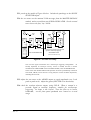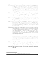
1
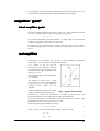
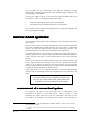
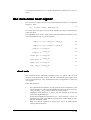
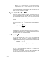
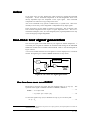
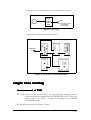
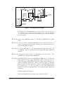
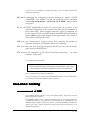
AMPLIFIER OVERLOAD
PREPARATION................................................................................. 44
not too little - not too much....................................................... 44
amplifier ‘gain’.......................................................................... 45
ideal amplifier ‘gain’................................................................................45
real amplifiers ..........................................................................................45
harmonic distortion ................................................................... 46
calculation of harmonic distortion components........................................46
definition of harmonic distortion - THD ..................................................47
measurement of THD ...............................................................................47
narrow band systems ................................................................. 48
measurement of a narrow band system.....................................................48
the two-tone test signal.............................................................. 49
short cuts ..................................................................................................49
signal-to-distortion ratio - SDR................................................................50
two-tone example .....................................................................................50
noise .......................................................................................... 51
two-tone test signal generation.................................................. 51
the two-tone seen as a DSBSC .................................................................51
EXPERIMENT ................................................................................... 52
experimental set-up ................................................................... 52
single tone testing...................................................................... 53
measurement of THD ...............................................................................53
two-tone testing......................................................................... 55
measurement of SDR................................................................................55
conclusions ................................................................................ 58
TUTORIAL QUESTIONS ................................................................. 58
APPENDIX......................................................................................... 59
some useful expansions............................................................. 59
Amplifier overload
Vol A2, ch 6, rev 1.1
- 43
AMPLIFIER OVERLOAD
ACHIEVEMENTS: an introduction to the definition and measurement of
distortion in wideband and narrowband systems.
PREREQUISITES: completion of the experiment entitled Spectrum analysis - the
WAVE ANALYSER in
this Volume.
EXTRA MODULES: SPECTRUM UTILITIES.
PREPARATION
not too little - not too much
One of the aims of an analog transmission system, such as an audio amplifier or a
long-distance telephone circuit, is to present at the output a faithful reproduction of
the signal at the input. Analog systems will always introduce some signal
degradation, however defined, but it is the aim of the analog design engineer to keep
the amount of degradation to a minimum.
As you are probably already aware, if signal levels within a system rise ‘too high’,
then the circuitry will overload; it is no longer operating in a linear manner. As will
be seen later in this experiment, extra, unwanted, distortion components will be
generated. These distortion, or noise 1, components, are signal-level dependent. In
this case the noise components arise due to the presence of the signal itself.
Conversely, if signal levels within a system fall ‘too low’, then the internal circuit
noise, which is independent of signal level, will eventually swamp the small, wanted,
output. The background noise of the TIMS system is held below about 10 mV peak
- this is a fairly loose statement, since this level is dependent upon the bandwidth
over which the noise is measured, and the model being examined at the time. A
general statement would be to say that TIMS endeavours to maintain a SNR of better
than 40 dB for all models.
Thus analog circuit design includes the need to maintain signal levels at a level 'not
to high' and 'not too low', to avoid these two extremes.
The TIMS working level, or ANALOG REFERENCE LEVEL has been set at
4 volts peak-to-peak. Modules will generally overload if this level is exceeded by
say a factor of two.
1 noise is here considered to be anything that is not wanted.
44 - A1
Amplifier overload
It is the purpose of this experiment to introduce you to the phenomenon of circuit
overload, and to offer some means of defining and measuring its effects.
amplifier ‘gain’
ideal amplifier ‘gain’.
Consider an amplifier which is said to have a gain of ‘g’. This is understood to mean
that, if vi is the input signal voltage, then the output vo is given by:
........ 1
v = g.v
o
i
This would be described as an ideal amplifier. Its input/output (i/o) characteristic
would be a straight line, with a slope of g volts/volt.
In simple terms, g is a dimensionless constant. More generally it can be complex,
and frequency dependent; but such complications will be ignored in the work to
follow.
real amplifiers
Unfortunately, a real amplifier does not have an ideal straight-line input/output
characteristic. It is more likely to look like that of Figure 1.
It is obvious to the eye that the
characteristic shown in Figure 1 could not
be considered straight, or linear, except
perhaps for input signal amplitudes in the
range say ± ½ volt.
In this range the slope of the characteristic
is 10 volts/volt.
The amplifier is said to have a small
signal gain of 10. Input signal amplitudes
in the range say ± ½ volt would be
considered small signals for this
amplifier.
A typical amplifier characteristic is likely
Fig 1: typical characteristic
to flatten off and become parallel to the
horizontal axis, whereas this characteristic, as defined by eqn. (2) below, will
approach and finally cross the input-axis for larger input amplitudes.
So this approximation to an amplifier characteristic should be used for input
amplitudes restricted to the range 0 to say ±1½ volts.
Its actual input/output relationship is given by:
vo = g1.vi + g3.vi3
........ 2
where vi and vo are the input and output voltages, respectively, and
Amplifier overload
g1 = 10
........ 3
g3 = - 1.5
........ 4
A1
- 45
Note that the range of the so-called linear part of the characteristic is not obvious
from a cursory examination of eqn. (2) alone. We shall later obtain a method of
defining an acceptable operating input signal range.
harmonic distortion
calculation of harmonic distortion components
Intuition tells us that an amplifier with the input-output characteristic of Figure 1 will
introduce distortion, but what sort of distortion ? This can be checked analytically
by nominating a test input signal, and then determining the corresponding output.
Let the test signal be a single tone, vi, where:
vi = V.cosµt
........ 5
Substituting this into eqn. (2), and expanding, gives:
........ 6
vo = g1 V cosµt + g3 V3 (3/4 cosµt + 1/4 cos3µt)
Notice that the cubic term has given rise to two new components; one on the same
frequency as the input signal, and the other on its third harmonic.
After combining like harmonic terms the last equation can be rewritten as:
........ 7
vo = [g1 V + (3/4) g3 V3] cosµt + (1/4) g3 V3 cos3µt
Notice that, at the output:
1) the amplitude of the wanted term cosµt is no longer simply g1 times the input
amplitude (as suggested by eqn. (1)).
2) there is an extra, unwanted term, on the third harmonic of the input.
The original signal has been distorted.
This can be observed in the time domain, using an oscilloscope. For the example
under discussion, the output, for an input of amplitude V = 1 volt, is shown in Figure
2.
Figure 2: the output voltage waveform of eqn. (7),
for an input amplitude of V = 1 volt
46 - A1
Amplifier overload
definition of harmonic distortion - THD
Notice that the analysis has been performed so as to describe the output in terms of
harmonic components of the input. The fundamental, or first harmonic, is the
wanted term, and all higher harmonic terms (in this example there is only one) are
unwanted.
The wanted and unwanted harmonic terms can be compared, and some measure
defined, to describe the amount of harmonic distortion.
The comparison is usually made on a power basis, described as the ‘total harmonic
distortion’, or THD, and defined as:
THD = 10 log10
∑H
∑H
2
1
n
dB
2
j
........ 8
j =2
where H1 is the amplitude of the output signal on the same frequency as the input test
signal, and the Hj are the amplitudes of the 2nd and higher harmonics, or unwanted,
terms.
Figure 3: THD versus input amplitude
for the response of eqn. (2)
For the example above, where the input amplitude V was 1 volt peak, this evaluates
to a THD of 27.48 dB.
Figure 3 shows the THD plotted for input amplitudes in the range 0 to 1½ volts.
Having decided on an acceptable THD for this amplifier (say 40 dB), the user can
now specify a maximum input level (½ volt) from Figure 3.
measurement of THD
There are instruments available which measure THD directly. They supply their
own test input signal to the device under test, measure the total AC power output,
subtract the power due to the wanted signal, and present the THD expressed in
decibels.
Amplifier overload
A1
- 47
You will make your own measurements with TIMS by modelling a WAVE
ANALYSER 2, measuring the amplitudes of the individual output components, and
then applying the THD formula.
Note that this THD is specific to the actual input signal amplitude used for the
measurement. There is no subsequent simple step to enable:
1.
2.
prediction of the THD for another input signal amplitude.
determination of the non-linear characteristic of the amplifier.
This is because of the non-linear relationship between the input signal amplitude and
the corresponding output THD.
narrow band systems
The previous discussion requires some modification if the system being examined is
narrow band 3.
There are many circuits in an analog communications system which are narrowband,
since many communications signals themselves are narrow band. A narrowband
system is one which has had its frequency response intentionally restricted. This
generally simplifies the circuit design, and eliminates out-of-band noise.
To simplify the discussion, suppose there is a bandpass filter at the system output, so
that only frequencies over a narrow range either side of the measurement frequency,
µ rad/s, will pass to the output. Let the non-linearities be in the circuitry preceding
the filter.
If this were the case for the example already discussed, the output waveform would
show no sign of distortion, but instead be a pure sinewave ! No distortion would be
visible on an oscilloscope connected to the output, because the distorting third
harmonic signal would not reach the output. An instrument for measuring THD with
a single tone input would register no distortion at all !
Is the system linear or not ? It is definitely non-linear. This can be demonstrated by
observing that the relationship between input amplitude and output amplitude is not
linear.
Using the methods so far employed, this does not
show up as waveform distortion, and would not be
revealed by a spectrum analysis of the output
measurement of a narrow band system
The single-tone test signal we have been using so far is inappropriate for the
measurement of THD in a narrow-band system. What is needed is a more
demanding test signal, which will reveal the non-linearity, and which is more
representative of the signals to be found in most systems. The non-linearity is
2 see the experiment entitled Spectrum Analysis - the Wave Analyser, or model a spectrum analyser
using the TIMS320 module.
3 ‘wideband’ and ‘narrowband’ signals are defined in the chapter entitled Introduction to Modelling
with TIMS.
48 - A1
Amplifier overload
revealed by the transmission of two signals simultaneously, namely the two tone test
signal.
the two-tone test signal
The two-tone test signal consists of two equal amplitude sinusoids, of comparable
frequency. Thus:
........ 9
v(t) = V (cosµ t + cosµ t) where say µ < µ
1
2
1
2
Let us use this as the input to the non-linear amplifier previously examined with a
single tone input.
The amplitudes of the various output terms, from trigonometrical expansion of v(t)
when substituted into eqn. (2), are shown below:
cos(µ1).t ==> g1.V + (3/4).g3.V3 + (3/2).g3.V3
........ 10
cos(µ2).t ==> g1.V + (3/4).g3.V3 + (3/2).g3.V3
........ 11
cos(3µ1).t ==> (1/4).g3.V3
........ 12
cos(3µ2).t ==> (1/4).g3.V3
........ 13
cos(2µ1 - µ2) t ==> (3/4).g3.V3
........ 14
cos(µ1 - 2µ2) t ==> (3/4).g3.V3
........ 15
cos(2µ1 + µ2) t ==> (3/4).g3.V3
........ 16
cos(µ1 + 2µ2) t ==> (3/4).g3.V3
........ 17
short cuts
The calculation of these amplitude coefficients can be very tedious. But one soon
observes certain phenomena involved, and with a narrowband system applies short
cuts to avoid unnecessary work. Remember that the two frequencies µ1 and µ2 are
close together.
Some observations are:
•
•
•
•
Amplifier overload
The trigonometrical expansions can only generate terms on harmonics of the
original frequencies, and on sum and difference frequencies of the form (n.µ1
+ m.µ2) and (n.µ1 - m.µ2), where n and m are positive integers.
Components with frequencies µ1 and µ2 will pass through the system, but
none of their higher harmonics.
Of the sum and difference frequencies (n.µ1 + m.µ2) and (n.µ1 - m.µ2), it is
agreed that only those of the difference group, where n and m differ by unity,
will pass through the system.
When n is odd, the expansion of (cosµt)n gives rise to all odd harmonics
counting down from the nth.
A1
- 49
•
When n is even, the expansion of (cosµt)n gives rise to all even harmonics
counting down from the nth. Note that the count goes down to the zeroeth
term, which is DC.
Taking these observations into account when dealing with a narrowband system, the
number of necessary calculations can be reduced.
signal-to-distortion ratio - SDR
We have seen that when the test input is a single tone, the distortion components are
restricted to being harmonics of this signal. But with a more complex test signal
other distortion products are possible. As has just been seen, a two-tone test input
gives rise to harmonics of each of these signals, as well as intermodulation products.
Intermodulation products (IPs) arise from the products of two or more signals, and
fall on frequencies which are the sums and differences of multiples of their
harmonics.
The measure of distortion can no longer be called THD, since the sum and difference
frequencies are present in addition to the harmonic terms, so the term signal-todistortion ratio, or SDR, is used. It is evaluated using the same principle as THD,
namely:
n
∑W
2
∑U
2
j
i
SDR = 10 log10
i =1
m
dB
........ 18
j =1
where the amplitude of the n wanted terms is Wi and of the m unwanted terms is Uj.
These are the terms which actually reach the output. In a narrow band system many
others will be generated which will not reach the output.
two-tone example
We will now apply eqn. (18) to calculate the SDR for the characteristic of Figure 1.
The input signal is defined by eqn. (9), with V = 0.5 volts. This makes the peak
amplitude of the two-tone signal equal to 1 volt, which is comparable with the
amplitude used earlier for the single tone testing. First we will include all unwanted
components in the calculation, making this a wideband result.
........ 19
wideband SDR = 27.01 dB
For the narrowband case the terms to be neglected, in this example, are those on the
third harmonics of µ1 and µ2 and the intermodulation products on the sum
frequencies. The result is then:
........ 20
narrowband SDR = 30.25 dB
Remember that, had a single tone been used for this narrowband system, there would
have been no signal-dependent distortion products found at the output, and the
amplifier would have appeared ideal.
The noise output would not, in fact, have been zero. We have been dealing with
large-signal operation, and so have ignored the existence of random noise.
50 - A1
Amplifier overload
noise
In the work above we have divided the output signal into wanted and unwanted
components. All the unwanted components so far had magnitudes which were
directly dependent upon the amplitude of the input signal. Such unwanted
components are referred to as signal dependent noise.
Also to be considered in any system is random noise, or system noise. This arises
naturally in all circuitry, and its magnitude is independent of any input signal 4.
In the work above we have made no mention of such noise. This is because it has
been assumed insignificant with respect to signal dependent noise. This was a
reasonable assumption, since, in a well designed system, signal dependent noise only
occurs for large input signal magnitudes.
two-tone test signal generation
The two-tone signal can be made from any two signals of suitable frequencies; a
convenient pair of signals for TIMS is the nominal 2 kHz message at the MASTER
SIGNALS module and an AUDIO OSCILLATOR. Refer to the block diagram of
Figure 4 below.
A lot can be learned about the two tone signal if it can be displayed in a convenient
manner. Recognising it as a form of DSBSC makes this an easy matter.
ENVELOPE
DETECTOR
µ
1
µ
2
ext. trig
TWO TONE
TEST
SIGNAL
Figure 4: two-tone test signal generation
the two-tone seen as a DSBSC
Recall that a two-tone test signal has been defined earlier as in eqn. (9). The
spectrum of this signal is identical with that of a DSBSC, defined as:
........ 21
DSBSC = 2.V.cosµt.cosωt
= V [cos(ω - µ)t + cos(ω + µ)t ]
........ 22
To force the signal of eqn. (21) to match that of eqn. (9), it is necessary that:
........ 23
ω-µ = µ
1
4 although it can be dependent on the presence of an input generator, the output impedance of which can
influence the system noise.
Amplifier overload
A1
- 51
........ 24
ω + µ = µ2
From these two equations the DSBSC frequencies are:
µ = ( | µ2 - µ1 | ) / 2
ω = ( µ1 + µ2 ) / 2
........ 25
rad/s
........ 26
rad/s
To display a DSBSC stationary on the screen a triggering signal is required that is
related to its envelope. The envelope of the DSBSC of eqn. (21) is a full wave
rectified version of cosµt, but there is no signal at this frequency [ eqn. (25) ] if the
two-tone signal is made by the addition of two tones as per eqn. (9).
The appropriate triggering signal can be generated with an envelope detector acting
on the two-tone signal. Remember this is a rectifier followed by lowpass filter which
will pass a few harmonics (ideally the first only) of the difference frequency of
eqn. (25), but not the sum frequency eqn. (26).
EXPERIMENT
experimental set-up
For this experiment you will need a WAVE ANALYSER. We suggest you use the
model examined in the experiment entitled Spectrum analysis - the WAVE
ANALYSER.
For the non-linear amplifier you will use the COMPARATOR within the UTILITIES
module. Please refer to the TIMS User Manual. The COMPARATOR has an
analog (YELLOW) output socket, which you will use, and in this application it is
called a CLIPPER. The CLIPPER has a non-linear input/output characteristic. That
is, it will overload with input signal amplitudes comparable with the TIMS
ANALOG REFERENCE LEVEL of 4 volts peak-to-peak.
The overload
characteristic can be varied by means of two on-board DIP switches. For the present
application you will use the ‘soft clipping’ characteristic; this is set with SW1
switched to ‘ON/ON’, and SW2 switched to ‘OFF/OFF’. The REF input socket,
used for the COMPARATOR, is not used for CLIPPER applications.
From now on the CLIPPER will be referred to as the
‘DUT’, namely the ‘device-under-test’.
For the purpose of the experiment you could consider it to be an amplifier in an
audio system, where it is required to amplify speech signals. Thus it is a wideband
device.
52 - A1
Amplifier overload
You should base your experimental set up on the block diagram of Figure 5.
DUT
device
under
test
test signal
OUT
to OSCILLOSCOPE
and WAVE
ANALYSER
Figure 5: test setup
The WAVE ANALYSER model is shown in Figure 6
UNKNOWN
IN
Figure 6: the WAVE ANALYSER model.
single tone testing
measurement of THD
T1 set the DIP switches on the DUT to the low gain (soft limiting) position,
before inserting the module into the TIMS SYSTEM UNIT. This is the
device under test (‘DUT’). Include the patchings to the SCOPE
SELECTOR inputs.
T2 patch up the model as in Figure 7 below.
Amplifier overload
A1
- 53
ext. trig
CH2-A
CH1-A
CH1-B
roving
lead
DEVICE
UNDER
TEST
#1
to WAVE
ANALYSER
#2
SINGLE TONE
TEST SIGNAL
Figure 7: the single tone test model
The ADDER, in cascade with BUFFER #2, will be used later in the two-tone test set
up. BUFFER #2 will be used for test signal amplitude control. The other BUFFER,
#1, is used for polarity reversal and level adjustment of the oscilloscope display of
the input test signal.
T3 set the gain of the ADDER to about ½, and that of BUFFER #2 to about
unity.
T4 use the ‘ext. trig’ from a constant amplitude version of the test source, as
shown, to trigger the oscilloscope. Set the sweep speed to show one or
two periods of the test signal.
T5 switch to CH1-A and CH2-A. Set both channels to the same gain, say
½ volt/cm. You are looking at both the input and output signals of
the DUT.
T6 use the oscilloscope shift controls to superimpose the two traces.
BUFFER #1 to equalize their amplitudes.
Use
T7 notice that BUFFER #2 varies the amplitude of both traces, so they stay
superimposed at low input amplitudes, before distortion sets in.
Adjust the gain of BUFFER #2 until the output signal indicates the
onset of moderate distortion; that is, when its shape is obviously
different from the input waveform, which is also being displayed on
the oscilloscope. A ratio of about 5:6 for the distorted and
undistorted peak-to-peak amplitudes gives a measurable amount of
distortion.
You have duplicated Figure 2.
Record the amplitude of the signal at the input to the DUT.
54 - A1
Amplifier overload
You are now set up moderate overload of the DUT. You are ready to measure the
distortion components.
T8 without disturbing the arrangement already patched up, model a WAVE
ANALYSER. For example, use the one examined in the experiment
entitled Spectrum analysis - the WAVE ANALYSER. This is shown
in Figure 6.
T9 use the WAVE ANALYSER to search for, and record, the presence of all
significant components at the output of the DUT for the conditions of
the previous Task. Theory suggests that these will be at 2.084 kHz (set
by the nominal 2 kHz test signal from the MASTER SIGNALS module)
and its odd multiples (odd, because of the approximate cubic shape of
the transfer function of the DUT).
T10 from your measurements of the previous Task calculate the amount of
harmonic distortion ( THD) under the above conditions.
T11 now reduce the level of the input signal to the DUT by (say) 50% (using the
gain control of BUFFER #2).
T12 measure the amplitude of the largest unwanted component - the third
harmonic of the input.
You should have observed that:
whereas the amplitude of the input was reduced by 50%, that
of the largest unwanted component fell by more than this.
This is a phenomenon of non-linear distortion.
Now try a two-tone test, looking for intermodulation products as well as harmonics.
You will work on the same amplifier (DUT) as before.
two-tone testing
measurement of SDR
If you built the model of Figure 7, then you are almost ready. The new test set-up is
illustrated in Figure 8 below.
The ADDER combines the two signals in equal proportions. The tones should be of
‘comparable frequency’; say within 10% or less of each other. BUFFER #2 at the
ADDER output is used as a joint level control. As before, BUFFER #1 enables the
‘before’ and ‘after’ signals, displayed on CH1-A and CH2-A respectively, to be
matched in amplitude.
Amplifier overload
A1
- 55
T13 patch up the model of Figure 8 below. Include the patchings to the SCOPE
SELECTOR inputs.
T14 the two tones are the nominal 2 kHz message from the MASTER SIGNALS
module, and a second from an AUDIO OSCILLATOR. Set the second
tone close to the first, say 1.8 kHz.
DUT output
CH2-A
DUT input
CH1-A
CH1-B
roving
lead
to WAVE
ANALYSER
ext. trig
DEVICE
UNDER
TEST
recovery of the envelope of the two-tone
signal for oscilloscope triggering
TWO-TONE GENERATOR
INSTRUMENTATION
(WAVE ANALYSER not shown)
Figure 8: two-tone test setup
The two-tone signal necessitates new oscilloscope triggering arrangements. As
already explained, an envelope recovery circuit is needed, and this is shown
modelled with a RECTIFIER in the UTILITIES module, and a TUNEABLE LPF.
Three of the four SCOPE SELECTOR positions are shown permanently connected.
The fourth, CH1-B, can be used as a roving lead, for various waveform inspections,
including the next task.
T15 adjust the two tones at the ADDER output to equal amplitudes (say 2 volt
peak-to-peak each). Adjust the gain of BUFFER #2 to about unity.
T16 check the envelope detector output, using CH1-B. What is wanted is a
periodic signal at envelope frequency, suitable for oscilloscope
triggering. Its shape is not critical. Tune the filter to its lowest
bandwidth; set the front panel passband GAIN control to its mid
range.
56 - A1
Amplifier overload
T17 when satisfied with the previous Task, use the output of the envelope detector
to trigger the oscilloscope, and check on CH1-A (with BUFFER #1 set
to mid-gain) that the envelope of the two-tone signal is stationary on
the screen (showing one or two periods of the envelope). Note that
this display will show up any imperfection in the equality of the
amplitudes of the two tones (or could have been used to set them equal
in the first place).
T18 switch to CH1-A and CH2-A. Set both these oscilloscope channels to the
same gain. You are now observing the input and output of the DUT.
Adjust the gain of BUFFER #2 so that the output (CH2-A) is not
distorted - that is, the same waveform as CH1-A.
T19 use the oscilloscope shift controls to overlay the two waveforms. Adjust the
gain of BUFFER #1 until they are of exactly the same amplitude, and
so appear as a single trace on the screen.
T20 now slowly increase the gain of BUFFER #2. Both traces will get larger,
but remain overlaid, until the signal level into the DUT exceeds its
linear operating range, and the output begins to show distortion. The
two waveforms will no longer be identical, and the difference should
be clearly visible.
T21 familiarize yourself with the overloading process by covering the full gain
range of BUFFER #2. Then set the gain to the point where distortion
of the DUT output waveform is ‘moderate’ 5. A ratio of output to
input signal amplitudes of about 5:6 is suggested as a start. This is
the condition under which you will be making some distortion
measurements. Record the input amplitude to the DUT; sketch the
input and output waveforms.
Remember the DUT has a cubic non-linearity. This suggests it will generate odd
order harmonic and intermodulation products. If the two test signals are f1 and f2,
then the largest unwanted components are likely to be on frequencies 3f1, 3f2,
(2f1±f2) and (2f2±f1).
T22 use the WAVE ANALYSER to search for, and record, the presence of all
significant components in the output of the DUT for the conditions of
the previous Task. Record clearly the frequency of each component
found, and relate it to the frequencies of the two-tone signal.
T23 from your measurements of the previous Task calculate the SDR, using
eqn. (18).
5 if you make it too slight the distortion components will be hard to find !
Amplifier overload
A1
- 57
In the above calculation you might have included all components which you
measured.
But suppose the output signal DUT had then been transmitted via a channel with a
bandpass characteristic. Then many of the distortion components would have been
removed.
But distortion would still have been measured, since those
intermodulation products close to the two wanted tones would have been passed.
T24 re-calculate the SDR, assuming transmission was via a bandpass filter.
conclusions
During the experiment you might have taken the opportunity to listen to the signals
with and without distortion, to gain a qualitative idea and appreciation of what level
of distortion - with these types of signals - is detectable by ear.
This experiment has served as an introduction to the methods of measuring and
describing the non-linear performance of an analog circuit. A problem associated
with the measurement of a narrowband system has been demonstrated, together with
a method of overcoming it.
TUTORIAL QUESTIONS
Q1 why were the two tones, in the two-tone test signal, set relatively close in
frequency to each other ?
Q2 equation (19) suggests an alternative method of making a two-tone test signal.
It has the particular advantage of providing a synchronizing signal
(from the low frequency source), the two tones are automatically of
equal amplitude, and the whole signal can be swept across the
spectrum with one control - that of the high frequency oscillator.
What are some disadvantages of this method of generation ?
Q3 explain qualitatively how the display of the two added tones, as a DSBSC
signal, can be used to equalize the amplitudes of the two tones. Use a
phasor diagram or other method to explain the process quantitatively.
Q4 two businesses advertise the same amplifier, one saying it is a 50 watt
amplifier, and the other a 60 watt amplifier. There is no dishonesty.
How could this be ?
58 - A1
Amplifier overload
APPENDIX
some useful expansions.
In analysing a non-linear system in terms of sinusoidal signals as in the above work,
the aim is to convert expressions in terms of powers of sinusoidal signals to
expressions in terms of harmonics of the fundamental frequencies involved.
Some useful expansions are:
cos2Α = 1/2 + 1/2.cos2Α
cos3Α = 3/4.cosΑ + 1/4.cos3Α
cos4Α = 3/8 + 1/2.cos2Α + 1/8.cos4Α
cos5Α = 5/8.cosΑ + 5/16.cos3Α + 1/16.cos5Α
cos6Α = 5/16 + 15/32.cos2Α + 3/16.cos4Α + 1/32.cos6Α
Perhaps you can see the pattern developing ? It is clear that:
•
•
when n is odd, the expansion of (cosmt)n gives rise to all odd harmonics
counting down from the nth.
when n is even, the expansion of (cosµt)n gives rise to all even harmonics
counting down from the nth. Note that the count goes down to the zeroeth
term, which is DC.
After an expression has been reduced to the sum of harmonic terms, those of similar
frequency must be combined, taking into account their relative phases. Thus:
V1.cosµ1t + V2.cosµ1t = ( V1 + V2 ).cosµ1t
but
V1.cosµ1t + V2.sinµ1t = V.cos(µ1t + α)
where
V = (V12 + V22 )
and
α = tan −1 (
V2
)
V1
As an exercise, develop the above expansions in terms of sin functions. There must
be some obvious similarities, but just as importantly there must be differences.
Explain !
Further useful expansions may be found in Appendix B to this Text.
Amplifier overload
A1
- 59
60 - A1
Amplifier overload