1
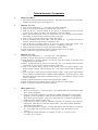
Tutorial session 4 examples
1.
ADF01 and ADF12
1. Explore the ADAS database for these formats. Note that the specification is in the IDLADAS User manual (appxa-01 and appxa-12).
2.
ADAS301 Test Case
2. Move to your sub-directory /.../<uid>/adas/pass. Start ADAS301.
3. Click on Central Data, and select qcx#h0/qcx#h0_old#n7.dat.
4. Click the Browse comments button to see the list of transitions present in the file
qcx#h0/qcx#h0_old#n7.dat. Move onto ADAS301 Processing window.
5. Select Fit polynomial at the 5% level. Click on the n=8 - n’=7 transition in the transition
list window. You will need to use the scroll-bar on the right.
6. Click on Select Velocities/Energies for Output File button.
7. Now put in default values in the Table. Note the units in use. It is preferred to units of
eV/amu. You need to edit the table to change the units.
8. Click on the Select Qunatum Numbers for Processing button. Select the 7f shell. Note
that you can select total and partial cross-sections – see the key to the right.
9. Click on the Done button to proceed to the Output options window.
10. Click on the button for Graphical Output. Then click Done to see the graph.
11. Have a look at the output text file after completion
3.
ADAS303 Test Case
12. Move to your sub-directory /.../<uid>/adas/pass. Start ADAS303.
13. Click on Central Data, and select qef93#h/qef93#h_c6.dat.
14. Click the Browse comments button to see what is in the file qef93#h_c6.dat. Move onto
ADAS303 Processing window.
15. Select Fit polynomial at the 5% level. Click on the n=8 - n’=7 transition in the transition
list window. You will need to use the scroll-bar on the right.
16. Click on the Default Energy/Velocity Values button. A set of energies appears in the
Output energies column. Note the units in use. You need to edit the table to change the
units.
17. Click on the Select supplementary plasma parameters button. Now type in Output Values
for Ion Density, Ion Temperature, Z effective and B Magnetic. Note the reference value
and valid ranges for each of these parameters are given. The reference values are good
values to start with.
18. Click on the Done button to proceed to the Output options window.
19. Click on the button for Graphical Output. Then click Done to see the graph.
20. Have a look at the output text file after completion
4
ADAS 308 Test Case
1. Move to your directory /.../<uid>/adas/pass. Start ADAS and move to the ADAS3 series
menu. Select ADAS308.
2. Click on Central Data, the data root to data class ADF01 should appear in the window
alongside. Click on the directory name qcx#h0 in the file list window. qcx#h0 appears
above in the selection window. Click on qcx#h0_old#n7.dat. It appears in the selection
window [you may need to scroll down].
3. Click the Browse comments button. Information of what is in the file qcx#h0_old#n7.dat
is displayed. Click Done to restore the Input window. Click Done and the ADAS308
Processing window appears.
4. The Processing window is complex. Note the information on donor and receiver near the
top. To the right enter the Atomic mass of the receiver (14.0). Remember to press
{return}.
5. Next Input the plasma parameters, for example, Ti=5.0e3, Te=5.0e3, Ni=2.5e13,
Ne=5.0e13, Zeff=2.0, B=3.0.
6.
Now Select charge exchange theory. This is a drop down menu. Click Use input data
set. [Note programs have built in default activation on some buttons. If the button is
darkened it is activated]. Now Select emission measure model. This is also a drop down
menu. Click Charge exchange.
7. Now turn to the Input of beam and spectrum line information and click first on the button
for Beam parameter information. The appropriate table appears below for editing.
Click Edit to bring up Table Editor and enter appropriate values, for example
0.85
8.0E4
0.12
4.0E4
0.03
2.7E4
and then Done.
8. Similarly, click the button for Observed spectrum lines and edit it’s table. Try
9
8
1.00E12
and click Done.
9. Finally click the button for Required emissivity prediction and edit it’s table. Try
9
8
1
8
7
2
7
6
2
6
5
and click Done.
10. All is now ready. Click Done to move to the Output options window.
11. Click the button for Graphical output. You may also Enable Hard Copy and Text Output.
Finally click Done to see the graph.
12. Click Done to return to the Output options screen. Click on the Exit to Menu icon to
finish up. Finally click on the Exit button on the sub-menu and main menu windows to
exit ADAS.
The tutorial continues with some examples concerned with beam stopping and beam emission.
5.
ADAS 304 Test Case
1. Move to your directory /.../<uid>/adas/pass. Start ADAS and move to the ADAS3 series
menu. Select ADAS304.
2. The Input window is different from the usual. Click on Central Data, the data root to the
data class ADF21 should appear in the window above. Now enter the Group name for
input files. This is the directory of the look-up tables of stopping data for a particular
beam species. Type bms93#h. Remember the {return}.
3. Now you must decide on the mixture of impurity nuclei (and hydrogen nuclei) which
cause the total stopping. Click the button Select Ion List. The button incidentally
becomes Reselect Ion List on later passes through. A button table pops up. Click on the
buttons for the nuclei you wish to include, for example, Be4, C6, H1 and click Done.
Note the Stopping Ion List. Click Done to advance to the Processing Options window.
4. Click on the Fit polynomial button, then type 5 in the adjacent active editable box
5. Now move to the Stopping ion fractions. Click on the Edit Table button to activate Table
Editor. Enter 0.1,0.1,0.8 for Be, C, H respectively and click Done.
6. Now Select the co-ordinate type for the output graph. Click the Energy button for the
first try.
7. Click on the Default Output Values button. You may find a warning widget pops up. If
so, click the Confirm button.
8. Click the button for Graphical output. Finally click Done to see the graph.
9. Click Done to return to the Output options screen. You may Exit to menu using the icon
in this program.
6.
ADAS 310 Test Case
1. Move to your directory /.../<uid>/adas/pass. Start ADAS and move to the ADAS3 series
menu. Select ADAS310.
2. The Input window is considerably different from the usual. Enter beam species details (H
for hydrogen and its isotopes) and the atomic charge of the beam species.
3. There are two files to be selected, the expansion file and the charge exchange file. To
select the expansion file, click on the Central Data button, the Data root to the data class
ADF18 should appear in the window above. Now select the data file bndlen_exp#h0.dat.
To select the charge exchange file, click on Central Data, the Data root to data class
ADF01 should appear in the window. Select qcx#h0. Now select the data file
qcx#h0_e2p#h1.dat. Click on the Done button to advance to the Proessing options
window.
4. The control parameters of the collisional-radiative calculation are organised into three
groups, selected in turn by the buttons general, switches (I) and switches (II).
General button: Click on the general button to view the general parameter settings.
The default values are reasonable.
Switches (I) button: Click on the switches (I) button to view the settings associated
with electron collisions. Working down the list set the parameters to the following: 2, 3,
NO, YES.
Switches (II) button: Click on the switches (II) button to view the settings associated
with the ion collisions. Working down the list set the parameters to the following: YES,
0, YES, YES.
5. Now you must decide what range of principal quantum numbers that you want to include
in the calculation. Click on the Representative N-shells button . Enter 1 and 110 as the
minimum and maximum n-shells. Now click on the Edit Table button and enter the
following values into the editor: 1,2,3,4,5,6,7,8,9,10,12,15,20,30,40,50,60,70,80,90,100.
Click on Done to return to the processing widget.
6. Now you need to decide the impurity content of the target plasma. Click on the Impurity
information button. Now click on the Selection mode button and choose Multiple
impurities. Click on the Edit Table button and enter the following information into the
editor
H
1.0
0.9
C
12.0
0.05
Be
11.0
0.05
Click on the Done button to return to the processing window.
7. Click on the electron/proton density scan button to choose the range of plasma densities.
In the usual manner enter the following values into the table editor.
8.
9.
1.0e13
1.0
2.0e13
2.0
3.0e13
3.0
4.0e13
4.0
5.0e13
5.0
Click Done to return to the processing window. Enter the value 3 as the Index for the
reference density.
Now click on the electron/proton temperature button and enter the following values ino
the text editor
1.0e3
2.0e3
3.0e3
4.0e3
5.0e3
Click on the Done button to return to the processing widget. Enter the value 3 as the
Index for the reference temperature.
Click on the beam energy scan button and eneter the following values into the table
editor
2.0e4
3.0e4
4.0e4
5.0e4
6.0e4
Click on the Done button to return to the processing widget. Ernter the value 3 for the
Index for the reference beam energy and 1.0e8 as the Beam density.
Now click on Done to advance to the Output window.
10. There are several possible outputs but our interest is in the contents of the first passing
file. The first passing file is of type ADF26 and contains the tabulated population
structure and effective stopping coefficients as a function of plasma parameters. It should
be noted that the fourth passing file contains the stopping coefficients assembled
according to format ADF21. The preferred route to obtaining the stopping coefficients is
via ADAS312.
11. Click on the First passing file button and enter a filename. Now click on Run now. An
Information widget appears. After the calculation, click on the Exit to Menu button to
return to the ADAS3 series menu.