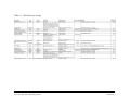
1
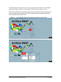
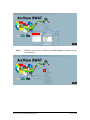
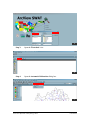
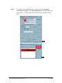
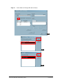
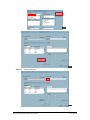
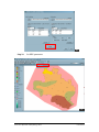
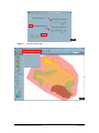
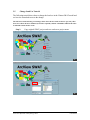
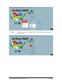
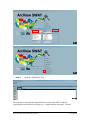
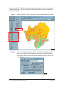
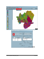
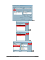
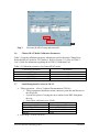
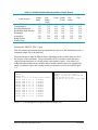
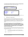
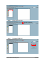
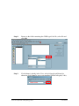
U.S. Army Corps of Engineers
Detroit District
Clinton River Watershed Model
User Manual
Prepared by
W.F. Baird & Associates Ltd.
Madison, Wisconsin
May 16, 2005
CLINTON RIVER WATERSHED MODEL
USER MANUAL
Prepared for:
US ARMY CORPS OF ENGINEERS
DETROIT DISTRICT
CONTRACT # DACW35-01-D-0009/0012
Prepared by:
W.F. BAIRD & ASSOCIATES
COASTAL ENGINEERS LTD.
MADISON, WI
MAY 16, 2005
USACE – Detroit District
Great Lakes Hydraulics and Hydrology Office
Clinton River Watershed Model
User Manual
Clinton River Watershed Model User Manual
For further information please contact
James P. Selegean, P.E,PhD.: (313)226-6791
This report was prepared by W.F. Baird & Associates Ltd. for USACE Detroit District.
The material in it reflects the judgment of Baird & Associates in light of the information
available to them at the time of preparation. Any use which a Third Party makes of this
report, or any reliance on decisions to be made based on it, are the responsibility of
such Third Parties. Baird & Associates accepts no responsibility for damages, if any,
suffered by any Third Party as a result of decisions made or actions based on this
report.
USACE – Detroit District
Great Lakes Hydraulics and Hydrology Office
Clinton River Watershed Model
User Manual
TABLE OF CONTENTS
1.0
INTRODUCTION ...................................................................................... 1
2.0
SWAT....................................................................................................... 1
2.1
System Requirements and Setup...............................................................................................1
2.2
Data Requirements.....................................................................................................................2
2.3
File Setup.....................................................................................................................................4
2.4
SWAT Set Up For Individual Subbasin Tutorial....................................................................4
2.5
Change Land Use Tutorial ......................................................................................................25
2.6
Clinton SWAT Model Calibration Parameters .....................................................................34
2.7
Land Management Practices in SWAT..................................................................................34
2.8
SWAT Output Description ......................................................................................................35
2.9
Future Developments ...............................................................................................................36
3.0
GSSHA................................................................................................... 37
3.1
The Project File (*.prj) ............................................................................................................37
3.2
The Index Map Tables .............................................................................................................39
3.3
GSSHA Land Use Change Tutorial........................................................................................45
3.4
Running GSSHA ......................................................................................................................53
3.5
GSSHA output interpretation .................................................................................................54
4.0
GIS PROJECTS...................................................................................... 55
5.0
REFERENCES ........................................................................................ 56
APPENDIX UM1 - SWAT PEER REVIEWED PUBLICATIONS
APPENDIX UM2 - INSTRUCTIONS TO INSTALL MANUAL GRID EDITOR
ARCVIEW EXTENSION
USACE – Detroit District
Great Lakes Hydraulics and Hydrology Office
Table of Contents
Clinton River Watershed Model
User Manual
1.0
INTRODUCTION
The following user manual is designed to complement the Clinton River Watershed
Sediment Transport Study Report (USACE, 2005) as well as the existing user manuals
for the numerical models (SWAT and GSSHA) used in the Clinton River Watershed
Modeling System. The following manual gives the users of the Clinton River watershed
models some additional information about the set up and execution of the SWAT and
GSSHA models as well as certain insight gained through the development of these
models for this specific watershed. In addition, the GIS projects set up for the Clinton
River Watershed Sediment Transport Study are introduced and explained.
Guidance on how to use the SWAT and GSSHA models, where they are applicable, as
well as example applications are given in USACE (2005), Sections 4 and 7.
2.0
SWAT
In addition to the accompanying report (USACE, 2005), the user has at their disposal
several documents pertaining to the SWAT model and AVSWAT interface (Di Luzio, et
al., 2001; Neitsch, et al., 2002a; Neitsch, et al., 2002b). It is assumed that the user will
utilize these documents as a guide for general SWAT model setup and execution. The
SWAT website also provides a list of SWAT peer reviewed publications. This list is
included in Appendix UM1. The following sections are designed to present some of the
most relevant information for getting started using the Clinton River SWAT model as
well as walk the user through some model modifications to ultimately rerun the SWAT
model to see the change in results. For this project, the ArcView interface (AVSWAT)
was used to set up and run the SWAT model, thus this manual will assume the user is
using the same.
2.1
System Requirements and Setup
The computer requirements and software setup for the Clinton River watershed SWAT
model are similar to those described in Section 2 of the AVSWAT User Guide. The
following system requirements are taken directly from the AVSWAT User Guide:
The SWAT2000/Arcview Interface requires:
• Personal computer using a Pentium I processor or higher, which
runs at 166 megahertz or faster
• 64 megabytes RAM minimum
• Microsoft Windows 95, 98, NT 4.0 or Win2000 operating system
with most recent kernel patch*
USACE – Detroit District
Great Lakes Hydraulics and Hydrology Office
1
Clinton River Watershed Model
User Manual
•
•
•
•
•
VGA graphics adapter and monitor. The interface works best
when the resolution is set to 800 x 600 or 1024 x 768 pixels, the
color palette is set to 8-bit (256 colors) or 16-bit (32768 colors)
and the display font size is set to small fonts.
50 megabytes free memory on the hard drive for minimal
installation and up to 300 megabytes for a full installation
ArcView 3.1 or 3.2 (software)
Spatial Analyst 1.1 or later (software)
Dialog Developer 3.1 or later (software – included with ArcView)
While 50 MB is adequate hard drive space for installing the interface, you
may need considerably more space to store the tables generated when the
interface processes the map layers.† We have found that a 2 gigabyte hard
drive works very well for storing ArcView, the SWAT/ArcView interface,
and project maps and tables.
Microsoft constantly updates the different versions of windows. This interface was
developed with the latest version of Windows and may not run with earlier versions.
Patches are available from Microsoft.
†
The space required to create a SWAT project with the SWAT/ArcView interface
depends on the resolution of the maps used. While testing the interface, a 10-meter
resolution DEM map layer taking up only 6 MB of space was processed. At one point in
the analysis of the map, the interface had filled 350 MB of storage with data.
*
An important note about the software requirements is that to use the AVSWAT interface
the user not only needs ArcView 3.X but also the Spatial Analyst Extension for ArcView,
which is a separate cost.
Section 2 of the AVSWAT User Guide (Di Luzio, et al., 2001) also provides instructions
on how to install the SWAT ArcView interface. The files used for installation can be
downloaded directly from the official SWAT website: http://www.brc.tamus.edu/swat/.
Order of installation:
1. ArcView 3.x
2. Spatial Analyst
3. AVSWAT
4. BASINS (optional – install if the user would like to use GenScn for output
processing)
2.2
Data Requirements
The required datasets are described in detail in the AVSWAT User Guide, Section 3.
The following is a summary of the datasets needed; in addition, comments are given to
further expand upon the requirements of certain datasets:
USACE – Detroit District
Great Lakes Hydraulics and Hydrology Office
2
Clinton River Watershed Model
User Manual
Required ArcView Map Themes:
• ArcInfo-ArcView GRID—Digital Elevation Model (DEM)
• ArcInfo-ArcView GRID or Shape—Land Cover/Land Use – the land cover/land
use is reclassified when brought in to AVSWAT, the user should double-check the
data table used for reclassification to be sure it corresponds correctly to their
dataset
• ArcInfo-ArcView GRID or Shape—Soil – AVSWAT is designed to use the NRCS
STATSGO soil dataset, though a pre-processor for the more detailed SSURGO
soil dataset has been developed at Texas A&M University and can be downloaded
at http://lcluc.tamu.edu/ssurgo/; the SWAT model developed for the Clinton River
watershed used the STATSGO soil dataset
• ArcInfo-ArcView GRID or Shape or Draw Manually—DEM Mask (optional)
• ArcInfo-ArcView Shape—Stream Delineation (optional)
The GIS datasets used in the Clinton River watershed SWAT model are listed in Table
4.1. It is important to remember that all GIS data sets must have the same projection to
use them in AVSWAT.
Required ArcView Tables and Text Files:
• Subbasin Outlet Location Table (dBase Table)
• Watershed Inlet Location Table (dBase Table)
• Land Use Look Up Table (dBase or ASCII) –the table developed for the Clinton
River watershed SWAT model for use with the NLCD land use dataset is given in
Table 2.1.
• Soil Look Up Table (dBase or ASCII)
• Weather Generator Gage Location Table (dBase)
• Precipitation Gage Location Table (dBase)
• Precipitation Data Table (dBase or ASCII)
• Temperature Gage Location Table (dBase)
• Temperature Data Table (dBase or ASCII)
• Solar Radiation, Wind Speed, or Relative Humidity Gage Location Table (dBase)
• Solar Radiation Data Table (dBase or ASCII)
• Wind Speed Data Table (dBase or ASCII)
• Relative Humidity Data Table (dBase or ASCII)
• Point Discharge Data Table—Annual Loadings (dBase or ASCII)
• Point Discharge Data Table—Monthly Loadings (dBase or ASCII)
• Point Discharge Data Table—Daily Loadings (dBase or ASCII)
• Reservoir Monthly Outflow Data Table (dBase or ASCII)
• Reservoir Daily Outflow Data Table (dBase or ASCII)
• Potential ET Data Table (dBase or ASCII)
USACE – Detroit District
Great Lakes Hydraulics and Hydrology Office
3
Clinton River Watershed Model
User Manual
It should be noted that most of these tables and text files are not necessary to set up a
simple SWAT model. Many are used to customize the model for special datasets or
measured inputs.
Table 2.1: Land use reclassification table for AVSWAT
SWAT Land
SWAT Land Cover/Plant
NLCD
NLCD Land Use Category
Cover/Plant Type
Type Description
code
11
Open Water
WATR
Water
21
Low Intensity Residential
URLD
Residential-Low Density
22
High Intensity Residential
URHD
Residential-High Density
23
Commercial/Industrial/Transportation
UCOM
Commercial
32
Quarries/Strip Mines/Gravel Pits
UIDU
Industrial
33
Transitional
RNGE
Range-Grasses
41
Deciduous Forest
FRSD
Forest-Deciduous
42
Evergreen Forest
FRSE
Forest-Evergreen
43
Mixed Forest
FRST
Forest-Mixed
81
Pasture/Hay
PAST
Pasture
82
Row Crops
AGRR
Agricultural Land-Row Crops
85
Urban/Recreational Grasses
AGRL
Agricultural Land-Generic
91
Woody Wetlands
WETF
Wetlands-Forested
92
Emergent Herbaceous Wetlands
WETN
Wetlands-Non-Forested
2.3
File Setup
All data and model files needed to run the Clinton River SWAT model are included on
the accompanying CD. In order to get the model to run properly please follow these
instructions:
•
•
•
Copy ClintonSWAT folder from the CD to c:\ drive.
Copy MI folder from CD to \\AVS2000\AvSwatDB\AllUs\statsgo.
Copy gridedit.avx from CD to \\ESRI\AV_GIS30\ARCVIEW\EXT32.
After each file or folder is copied, be sure to uncheck Read Only in the properties dialog
for each file/folder. If the files are left as “Read Only” the SWAT model will not run
properly.
In the following tutorials, some folder locations (pathnames) may be different from what
the user will have on their computer, depending on what drive the SWAT model was
installed.
2.4
SWAT Set Up For Individual Subbasin Tutorial
USACE – Detroit District
Great Lakes Hydraulics and Hydrology Office
4
Clinton River Watershed Model
User Manual
The following tutorial shows how to set up the Clinton SWAT model for an individual
subbasin by starting with the overall watershed SWAT model (clintonws.swat).
The red boxes on the following screen images show where the user needs to click or type; the yellow
boxes are to draw the user’s attention (no action is required); and the red numbers indicate the
order in which the actions need to occur.
Step 1:
Copy original SWAT project and save under new project name.
1
2
USACE – Detroit District
Great Lakes Hydraulics and Hydrology Office
5
Clinton River Watershed Model
User Manual
3
Step 2:
When the copy process is finished, click Open Project to open the newly
created project.
4
USACE – Detroit District
Great Lakes Hydraulics and Hydrology Office
6
Clinton River Watershed Model
User Manual
5
Step 3:
Open the Watershed view.
6
Step 4:
Open the Automatic Delineation dialog box.
7
USACE – Detroit District
Great Lakes Hydraulics and Hydrology Office
7
Clinton River Watershed Model
User Manual
Step 5:
To mask the desired subbasin area, click the box next to Focusing
watershed area option. Click Manually delineate, though other options
are available. Click No when asked to Edit the previous shape of mask
area.
8
2
1
9
USACE – Detroit District
Great Lakes Hydraulics and Hydrology Office
8
Clinton River Watershed Model
User Manual
Step 6:
Draw a line around the desired subbasin (in the case the Paint Creek
subbasin) using the Draw tool. This will create a mask so only the
portion of the DEM within this area will be processed – this saves
processing time.
10
USACE – Detroit District
Great Lakes Hydraulics and Hydrology Office
9
Clinton River Watershed Model
User Manual
Step 7:
Click Apply to process DEM.
11
12
13
USACE – Detroit District
Great Lakes Hydraulics and Hydrology Office
10
Clinton River Watershed Model
User Manual
Step 8:
Set threshold area for subbasins and click Apply to create stream
network. The smaller the number, the more detailed the stream network
generated.
1
2
14
USACE – Detroit District
Great Lakes Hydraulics and Hydrology Office
11
Clinton River Watershed Model
User Manual
Step 9:
To determine location for outlet of basin, open the USGS gage shapefile
and add an outlet at the gage location. This allows for direct comparison
of SWAT output to gage measurements.
15
16
USACE – Detroit District
Great Lakes Hydraulics and Hydrology Office
12
Clinton River Watershed Model
User Manual
Step 10:
Select gage location for whole watershed outlet.
17
2
1
18
USACE – Detroit District
Great Lakes Hydraulics and Hydrology Office
13
Clinton River Watershed Model
User Manual
19
Step 11:
After watersheds have been delineated, click Apply to calculate subbasin
parameters.
20
Step 12:
From the AVSWAT menu, select Land Use and Soil Definition.
21
USACE – Detroit District
Great Lakes Hydraulics and Hydrology Office
14
Clinton River Watershed Model
User Manual
Step 13:
Select Land Use layer.
22
2
1
23
2
1
24
2
1
25
USACE – Detroit District
Great Lakes Hydraulics and Hydrology Office
15
Clinton River Watershed Model
User Manual
Step 14:
Select land use lookup table and reclassify.
26
2
1
27
2
1
28
USACE – Detroit District
Great Lakes Hydraulics and Hydrology Office
16
Clinton River Watershed Model
User Manual
2
1
29
30
Step 15:
Select soils layer.
31
USACE – Detroit District
Great Lakes Hydraulics and Hydrology Office
17
Clinton River Watershed Model
User Manual
2
1
32
2
1
33
2
1
34
1
2
35
USACE – Detroit District
Great Lakes Hydraulics and Hydrology Office
18
Clinton River Watershed Model
User Manual
36
Step 16:
Set HRU parameters.
37
USACE – Detroit District
Great Lakes Hydraulics and Hydrology Office
19
Clinton River Watershed Model
User Manual
2
1
3
4
38
Step 17:
Specify climate data.
39
USACE – Detroit District
Great Lakes Hydraulics and Hydrology Office
20
Clinton River Watershed Model
User Manual
40
2
1
41
42
USACE – Detroit District
Great Lakes Hydraulics and Hydrology Office
21
Clinton River Watershed Model
User Manual
2
1
43
44
45
USACE – Detroit District
Great Lakes Hydraulics and Hydrology Office
22
Clinton River Watershed Model
User Manual
Step 18:
Write input files.
46
47
48
Step 19:
Run SWAT simulation.
49
USACE – Detroit District
Great Lakes Hydraulics and Hydrology Office
23
Clinton River Watershed Model
User Manual
1
2
3
50
51
52
USACE – Detroit District
Great Lakes Hydraulics and Hydrology Office
24
Clinton River Watershed Model
User Manual
2.5
Change Land Use Tutorial
The following tutorial shows how to change the land use in the Clinton SWAT model and
see how the watershed reacts to the change.
The red boxes on the following screen images show where the user needs to click or type; the yellow
boxes are to draw the users attention (no action is required); and the red numbers indicate the order
in which the actions need to occur.
Step 1:
Copy original SWAT project and save under new project name.
53
54
USACE – Detroit District
Great Lakes Hydraulics and Hydrology Office
25
Clinton River Watershed Model
User Manual
55
Step 2:
When the copy process is finished, click Open Project to open the newly
created project.
56
USACE – Detroit District
Great Lakes Hydraulics and Hydrology Office
26
Clinton River Watershed Model
User Manual
57
58
Step 3:
Open the “Watershed” view.
59
The next step is to modify the original land use used for the SWAT model or
create/import a new land use coverage (e.g., a future land use coverage). For this
USACE – Detroit District
Great Lakes Hydraulics and Hydrology Office
27
Clinton River Watershed Model
User Manual
exercise, the SWAT Land Use grid will be modified using an ArcView extension called
“Manual Grid Editor”. Refer to Appendix UM2 for instructions on how to install this
ArcView extension.
Step 4:
Make the SWAT Land Use grid active and open the Manual Grid Editor.
2
1
60
Step 5:
Select area of land use grid to modify. The Manual Grid Editor allows
the user to modify the whole grid or just a portion (using the graphics
tools) and to change the selected area to multiple land use values or one
single value.
61
USACE – Detroit District
Great Lakes Hydraulics and Hydrology Office
28
Clinton River Watershed Model
User Manual
For this example a polygon will be used to change the land use in the
selected area to low intensity residential (grid code = 21). The first click
will initiate the polygon, and to complete the polygon, hold down the
“Ctrl” key while clicking the final point or double-click on the final point.
2
1
4
5
3 – Draw
Polygon
62
USACE – Detroit District
Great Lakes Hydraulics and Hydrology Office
29
Clinton River Watershed Model
User Manual
63
Step 6:
Select newly modified land use grid (“Modified Grid”) for use in SWAT
model.
USACE – Detroit District
Great Lakes Hydraulics and Hydrology Office
30
Clinton River Watershed Model
User Manual
64
65
USACE – Detroit District
Great Lakes Hydraulics and Hydrology Office
31
Clinton River Watershed Model
User Manual
2
1
66
2
1
67
2
1
68
USACE – Detroit District
Great Lakes Hydraulics and Hydrology Office
32
Clinton River Watershed Model
User Manual
69
2
1
70
2
1
71
2
1
72
USACE – Detroit District
Great Lakes Hydraulics and Hydrology Office
33
Clinton River Watershed Model
User Manual
1
2
73
Step 7:
2.6
Proceed with SWAT setup and run model.
Clinton SWAT Model Calibration Parameters
Table 2.2 lists the calibration parameter adjustments used for the entire Clinton River
Watershed SWAT model for 1992 land use. Refer to Section 13.3 of the AVSWAT
User’s Guide for information regarding the AVSWAT Calibration Tool.
Table 2.2 Calibration parameters for Clinton SWAT model.
Calibration Parameter
CN2
ALPHA_BF
ESCO
REVAPMN
2.7
Adjustment
-4
+0.5
+0.95
+50
Land Management Practices in SWAT
•
•
Tillage operations – refer to Technical Documentation (TD) 20.6
o Tillage operation redistributes residue, nutrients, pesticides and bacteria in
the soil profile.
o User has the option of varying the curve number in the HRU throughout
the year.
o From Table 4 in Kirsch, et al. (2002)
Transect Survey Residue
Assumed SWAT Tillage Practice
Conventional (<15% cover)
Moldboard plow
Other (15% to 30% cover)
2 passes with chisel plow
Mulch (>30% cover)
1 pass with chisel plow
No-till
No-till
Filter strips – refer to TD 20.10
USACE – Detroit District
Great Lakes Hydraulics and Hydrology Office
34
Clinton River Watershed Model
User Manual
•
•
•
•
2.8
o Edge-of field filter strips may be defined in an HRU.
o Sediment, nutrient, pesticide and bacteria loads in surface runoff are
reduced as the surface runoff passes through the filter strip.
Riparian buffer areas – refer to Vaché, et al. (2002)
o Adjust channel cover factor and channel erodibility factor.
Irrigation – refer to TD 21.1
o Irrigation in an HRU may be scheduled by the user or automatically
applied by SWAT.
o In addition to specifying the timing and application amount, the user must
specify the source of irrigation water.
Infiltration – refer to TD 22.1 & 22.2
o User can specify fraction of impervious area, fraction of directly
connected impervious area and curve number for urban land types.
o Hydraulic conductivity can also be altered.
o Use Green & Ampt method and sub-daily precipitation to directly model
infiltration.
Street sweeping in urban areas – refer to TD 22.4.1
o Sweep operations impact build up of solids in the impervious portion of
the HRU.
o SWAT performs street sweeping operations only when the build up/wash
off algorithm is specified for urban loading calculations.
o
SWAT Output Description
Every SWAT simulation generates a number of output files including:
• The summary output file (output.std),
• The HRU output file (.sbs),
• The subbasin output file (.bsb) and
• The main channel or reach output file (.rch)
These are ASCII text files that can be viewed using any text editor. These files
(excluding output.std) can also be imported into ArcView. After the SWAT model is
run, a dialog box will appear asking if the user wants to read the ASCII outputs. If “yes”
is selected, AVSWAT will create .dbf table files from the ASCII text outputs, import
them into the ArcView project and open them. The user then has the option to use the
Map-Chart tool under the Reports menu to plot the SWAT results.
Chapter 32 of the SWAT User’s Manual (Neitsch, 2002a) explains in detail the primary
output files and the information they contain. Descriptions of the most relevant output
variables for the Clinton River SWAT model are described below.
USACE – Detroit District
Great Lakes Hydraulics and Hydrology Office
35
Clinton River Watershed Model
User Manual
Subbasin Output File (basins.bsb)
This file contains summary information for each subbasin in the watershed.
Variable Name
PRECIP
Description____________________________________________
Total amount of precipitation falling on the subbasin during a time
step (mm H2O).
SURQ
Surface runoff contribution to streamflow during a time step (mm
H2O).
GW_Q
Groundwater contribution to streamflow (mm). Water from the
shallow aquifer that returns to the reach during a time step.
WYLD
Water yield (mm H2O). The net amount of water that leaves the
subbasin and contributes to streamflow in the reach during a time
step.
SYLD
Sediment yield (metric tons/ha). Sediment from the subbasin that
is transported into the reach during a time step.
Main Channel Output File (basins.rch)
This file contains summary information for each routing reach in the watershed.
Variable Name
FLOW_IN
Description____________________________________________
Average daily streamflow into reach during a time step (m3/s).
FLOW_OUT
Average daily streamflow out of reach during a time step (m3/s).
SED_IN
Sediment transported with water into reach during a time step
(metric tons).
SED_OUT
Sediment transported with water out of reach during a time step
(metric tons).
SEDCONC
Concentration of sediment in reach during a time step (mg/L).
2.9
Future Developments
An ArcView 8.x interface for SWAT is currently under development by Francisco
Olivera and others at Texas A&M University. It is compatible with the ArcHydro data
model, a standard data model for spatial and temporal hydrologic data, thus enabling
more integration with other hydrologic and hydraulic models that use the same types of
input data. Since ESRI (the developer of the ArcView software) is no longer updating
the ArcView 3.x software, there is a general trend away from ArcView 3.X and towards
ArcView 8.X (and 9.X).
USACE – Detroit District
Great Lakes Hydraulics and Hydrology Office
36
Clinton River Watershed Model
User Manual
3.0
GSSHA
GSSHA is a physically-based, distributed-parameter model that simulates the hydraulic
response of watersheds to a given hydrometeorological condition.
The major
components of the model include:
•
•
•
•
•
•
•
•
•
•
Precipitation (spatial and temporal variation)
Precipitation interception
Snow fall accumulation and melting
Infiltration
Evapotranspiration
Overland flow routing
Groundwater flow
Channel routing
Overland Sediment erosion / deposition
In-stream sediment transport
A detailed description of how these processes are treated within the model are described
in USACE (2005), the GSSHA users manual developed by Downer and Ogden (2002)
and the folloing page fromn the Coastal and Hydraulics Laboratory CHL from the
USACE. http://chl.erdc.usace.army.mil/gssha .
This manual was designed to help Clinton watershed managers in the application and
interpretation of GSSHA numerical model and is organized by different processes. For
simplicity and because the events modeled were during the summer months,
evapotranspiration and snowfall accumulation and melting were not included in the
simulation process.
There are two main files that the user needs to understand in order to run GSSHA
properly: The project file and the Index map tables.
3.1
The Project File (*.prj)
This file contains the main information to run GSSHA which includes the file names for
all the parameters and basic information regarding grid size, time step etc. Figure 3.1
depicts a typical project file. The user should NOT change the red lines or “cards”.
MAP_FREQ and HYD_FREQ specify the frequency (in number of time steps) for file
output writing.
USACE – Detroit District
Great Lakes Hydraulics and Hydrology Office
37
Clinton River Watershed Model
User Manual
CASC2DPROJECT
WMS 6.1
WATERSHED_MASK
FLINE
METRIC
GRIDSIZE
ROWS
COLS
TOT_TIME
TIMESTEP
OUTROW
OUTCOL
OUTSLOPE
MAP_FREQ
HYD_FREQ
MAP_TYPE
CHAN_EXPLIC
SED_POROSITY
ELEVATION
DEPTH
INCLUDE_CHANNEL_DEPTH
INF_DEPTH
CHAN_DEPTH
CHAN_DISCHARGE
CHANNEL_INPUT
LINKS
NODES
DIS_PROFILE
WAT_SURF_PROFILE
OVERTYPE
INF_REDIST
MAPPING_TABLE
MATERIALS
GW_SIMULATION
AQUIFER_BOTTOM
WATER_TABLE
GW_HYCOND_MAP
GW_POROSITY_MAP
GW_BOUNDFILE
GW_TIMESTEP
GW_LSOR_DIR
GW_LSOR_CON
GW_RELAX_COEFF
GW_LEAKAGE_RATE
GW_INIT_MOISTURE
SUMMARY
OUTLET_HYDRO
OUTLET_SED_FLUX
PRECIP_FILE
SOIL_EROSION
SAND_SIZE
SILT_SIZE
CLAY_SIZE
WATER_TEMP
BRIEF DESCRIPTION
paint8_gar17k.msk
paint8_gar17k.map
49.829661
257
267
5760
20
256
255
0.001000
360
180
1
0.400000
paint8_gar17k.ele
paint8_gar17k.dep
paint8_gar17k
paint8_gar17k.cdp
paint8_gar17k.cdq
paint8_gar17k.cip
paint8_gar17k.lks
paint8_gar17k.nod
paint8_gar17k.qpf
paint8_gar17k.wpf
ADE
paint8_gar17k.cmt
paint8_gar17k.mat
paint8_gar17k.aqe
paint8_gar17k.wte
paint8_gar17k.hdc
paint8_gar17k.gwp
paint8_gar17k.bnd
60.000000
2
0.000010
1.200000
0.000000
0
paint8_gar17k.sum
paint8_gar17k.hyd
paint8_gar17k.sed
paint8_gar17k.gag
Infiltration depth (Output)
Channel depth (Output)
Channel Discharge (Output)
Channel network connectivity
Location of channel links
Location of channel nodes
Startup channel discharge
Startup channel discharge
Overland flow scheme
Infiltration method
Mapping table values
Material index
Aquifer bottom elevation
Water table elevation map
GW hydraulic Conductivity
GW porosity map
GW boundary map
Ground water time step
GW flow direction
Convergence parameter
Relaxation coefficient
GW leakage rate
GW Initial moisture
Summary file (output)
Outlet hydrograph
Outlet sediment flux
Precipitation time series
Sand size (mm)
Silt size (mm)
Clay size (mm)
Water temperature Cº
0.250000
0.016000
0.001000
20.000000
USACE – Detroit District
Great Lakes Hydraulics and Hydrology Office
Defines domain extension
River network
Units
Grid size spacing (m)
Number of grid squares in Y
Number of grid squares in X
Modeling time (minutes)
Time step (s)
Outlet Y location
Outlet X Location
Outlet slope
Map frequency output
Hydrograph frequency output
Type of output file 1=ASCII
Modeling scheme
Initial sediment porosity %
Surface elevation map (m)
Overland flow depth (Output)
38
Clinton River Watershed Model
User Manual
Figure 3.1 Project file sample (Do not modify red cards)
The ground water time step GW_TIMESTEP can be larger than the overland flow time
step. It is recommended that a multiple of the latter be chosen.
WATER_TEMP can be changed but only a constant value can be specified.
3.2
The Index Map Tables
MAPPING_TABLE (*.cmt)
This file contains index data information mainly associated with land use and soil type
raster data coverages. Each attribute is assigned with an index value for which different
erodability and infiltration parameters can be manipulated. The data shown in Figure 3.2
depicts an example of a mapping table file.
Each raster map is identified as an index map (*.idx), which is used for different
processes throughout the modeling. For example, the land use index map is used to
define friction parameters and the soil index map to define infiltration characteristics.
For erosion processes, the combination of soil type and land use maps will determine the
eroded material quantities.
Roughness (SURF_ROUGH)
This map defines the surface roughness of the model domain. A constant value could be
applied to the whole domain but it is more realistic to specify different values for
different land use types. For example, paved areas would have a much smaller friction
coefficient than densely vegetated areas. The Manning’s n values usually range from
0.005 to 0.7 depending on the land use type (see Table 3.1 for values). These values can
be manipulated within a reasonable range to calibrate the model.
Infiltration (GREEN_AMPT_INFILTRATION)
This parameter is associated mainly with soil type, although in some instances (especially
in smaller scale models) land use can play a significant role (e.g. infiltration rate would
be different for a driveway than for a lawn regardless of the soil type).
The main parameters considered in this map are:
Hydraulic conductivity (HYDR_COND)
Capillary Head (CAPIL_HEAD)
Porosity (POROSITY)
Pore distribution index (PORE_INDEX)
Residual water content (RESID_SAT)
The most sensitive parameters are the hydraulic conductivity and the capillary head, both
of which are used for calibration purposes.
USACE – Detroit District
Great Lakes Hydraulics and Hydrology Office
39
Clinton River Watershed Model
User Manual
Initial moisture (GREEN_AMPT_INITIAL_SOIL_MOISTURE)
The initial soil moisture can also be specified in SOIL_MOISTURE and it is dependent
on the soil type. For this case an assumed value of 0.38 (38% moisture) is used.
Soil Erosion properties (SOIL_EROSION_PROPS)
This erodability parameter is directly related to the soil properties, which include an
erodability factor (ERODABILITY), the sand percentage (SAND_PCT) and silt
percentage (SILT_PCT) of a particular soil type.
Soil Erosion Factors (SOIL_EROSION_FACTORS)
This set of parameters is related to the land use properties and accounts for management
practices through the C (CROP_MANAG) and P (CONS_PRAC) factors described by
the USLE equation. Although the C factor is fairly well defined in the literature and
digital data attributes for different land use types, this value can be manipulated to
calibrate the model in terms of sediment delivery.
Ground Water Properties
There are four raster maps associated with the ground water flow. All have a similar
structure and are described below:
Aquifer Bottom (*.aqe)
This file can be a constant number set to the elevation at which the bedrock is
encountered. Since in many instances this is an unknown value, it can be assumed to be
at a constant level below the surface. For this case it was assumed to be at 100m.
Water Table (*.wte)
This file contains water table elevation values for each grid cell. Since it is often
unknown, an arbitrary value can be assumed (e.g. 10 m below the surface), giving the
water table a parallel surface to the elevation map with a fixed vertical displacement.
This file influences base flow significantly, thus it can be manipulated to obtain better
calibration results. After the model is run, a “hotstart_file” is created which contains a
newer more natural water table level. This information can be cut and pasted into the
original *wte file. It is our experience that when the model is run for two or more cycles
the simulated water table levels produce results closer to measurements. Since the water
table is a function of the precipitation history, it is recommended that for each
precipitation event to be run by the user, the water table be adjusted to match the preevent outflow discharge.
Ground Water Hydraulic Conductivity (*.hdc)
This raster map defines the speed at which the groundwater moves in the horizontal
plane. The values are associated with the soil properties and can vary throughout the
domain. Typical values range from 10 to 40 cm/hr. The hydraulic conductivity is an
important parameter for calibration of the base flow. For this case the ground water
hydraulic conductivity was assumed constant.
USACE – Detroit District
Great Lakes Hydraulics and Hydrology Office
40
Clinton River Watershed Model
User Manual
GSSHA_INDEX_MAP_TABLES
INDEX_MAP
id_map_3.idx "land use"
INDEX_MAP
id_map_4.idx "soils"
INDEX_MAP
id_map_5.idx "infiltration"
ROUGHNESS "land use"
NUM_IDS 11
ID
DESCRIPTION1
DESCRIPTION2
2
Roughness ID
Residential
3
Roughness ID
Developed Industrial
8
Roughness ID
Bare Field
9
Roughness ID
Range (natural)
10
Roughness ID
Range (Clipped)
14
Roughness ID
Small Grain
15
Roughness ID
Row Crops
18
Roughness ID
Short GrassPrairie
22
Roughness ID
Forest
25
Roughness ID
Lakes
26
Roughness ID
Wetlands
INTERCEPTION ""
NUM_IDS 0
ID
DESCRIPTION1
DESCRIPTION2
RETENTION ""
NUM_IDS 0
ID
DESCRIPTION1
DESCRIPTION2
GREEN_AMPT_INFILTRATION "infiltration"
NUM_IDS 8
ID
DESCRIPTION1
DESCRIPTION2
2
Infiltration ID
Concreete/Asphalt
3
Infiltration ID
Developed/ Industrial (Loamy Sand)
4
Infiltration ID
Range/Forest/Prairie (Loamy Sand)
5
Infiltration ID
Crops (LoamySand)
6
Infiltration ID
Lakes Wetlands
8
Infiltration ID
Developed/ Industrial (Sandy Loam)
9
Infiltration ID
Range/Forest/Prairie (Sandy Loam)
10
Infiltration ID
Crops (SandyLoam)
GREEN_AMPT_INITIAL_SOIL_MOISTURE "soils"
NUM_IDS 2
ID
DESCRIPTION1
DESCRIPTION2
2
Soil Moisture ID
Sandy Loam
4
Soil Moisture ID
Loamy Sand
RICHARDS_EQN_INFILTRATION_BROOKS ""
NUM_IDS 0
MAX_NUMBER_CELLS 0
ID
DESCRIPTION1
DESCRIPTION2
RICHARDS_EQN_INFILTRATION_HAVERCAMP ""
NUM_IDS 0
MAX_NUMBER_CELLS 0
ID
DESCRIPTION1
DESCRIPTION2
EVAPOTRANSPIRATION ""
NUM_IDS 0
ID
DESCRIPTION1
DESCRIPTION2
SOIL_EROSION_PROPS "soils"
NUM_IDS 2
ID
DESCRIPTION1
DESCRIPTION2
2
Soil erosion properties ID
Sandy Loam
4
Soil erosion properties ID
Loamy Sand
SOIL_EROSION_FACTORS "land use"
NUM_IDS 11
ID
DESCRIPTION1
DESCRIPTION2
2
Soil erosion factors ID
Concreete/Asphalt
3
Soil erosion factors ID
Developed/ Industrial
8
Soil erosion factors ID
Bare Field
9
Soil erosion factors ID
Range (Natural)
10
Soil erosion factors ID
Range (Clipped)
14
Soil erosion factors ID
Small Grain
15
Soil erosion factors ID
Row Crops
18
Soil erosion factors ID
Short Grass Prairie
22
Soil erosion factors ID
Forest
25
Soil erosion factors ID
Lakes
26
Soil erosion factors ID
Wetlands
MATERIAL_INDEX
NUM_IDS 0
ID
DESCRIPTION
AQUIF BTM
WATER TBL
SURF_ROUGH
0.011000
0.013700
0.050000
0.130000
0.100000
0.150000
0.100000
0.150000
0.192000
0.400000
0.400000
STOR_CAPY
INTER_COEF
RETENTION_DEPTH
HYDR_COND
0.076000
0.836000
1.068000
6.004000
15.000000
0.185000
0.235000
1.326000
CAPIL_HEAD
6.130000
6.130000
6.130000
6.130000
6.130000
11.010000
11.010000
11.010000
POROSITY
0.401000
0.401000
0.401000
0.401000
0.401000
0.434000
0.434000
0.434000
PORE_INDEX
0.553000
0.553000
0.553000
0.553000
0.553000
0.252000
0.252000
0.252000
RESID_SAT A_REDUX_DEPTH
0.035000
0.000000
0.035000
0.000000
0.035000
0.000000
0.035000
0.000000
0.035000
0.000000
0.027000
0.000000
0.027000
0.000000
0.027000
0.000000
HYD_COND
POROSITY
RESID_SAT
SOIL_MOIST
WILTING_PT
DEPTH
LAMBDA
BUB_PRESS
DELTA_Z
HYD_COND
POROSITY
RESID_SAT
SOIL_MOIST
WILTING_PT
DEPTH
ALPHA
BETA
AHAV
ALBEDO
WILTING_PT
VEG_HIEGHT
ERODIBILITY
0.270000
0.120000
SAND_PCT
0.650000
0.800000
SILT_PCT
0.250000
0.150000
CROP_MANAG
0.005000
0.003000
0.300000
0.010000
0.010000
0.070000
0.120000
0.003000
0.011000
0.000100
0.001000
CONS_PRACT
0.400000
0.400000
0.400000
0.400000
0.400000
0.400000
0.400000
0.400000
0.400000
0.400000
0.400000
SOIL_MOISTURE
0.380000
0.380000
GW HYCOND GW POROSITY
BHAV
DELTA_Z
V_RAD_COEF CANOPY_RESIST
CELL ELEV
Figure 3.2 Index-Map-Tables File Sample.
USACE – Detroit District
Great Lakes Hydraulics and Hydrology Office
41
Clinton River Watershed Model
User Manual
Ground Water Porosity (*.gwp)
This file contains the initial porosity of the soil (1.0 being the highest value).
Table 3.1. GSSHA Surface Roughness Coefficients for Overland Flow (All Models)
Paint Creek
Galloway Creek
Middle Branch
Land Use Type
ID
Value
ID
Value
ID
Value
Residential
2
0.011
12
0.011
12
0.011
Developed/ Industrial
3
0.0137
13
0.0137
13
0.0137
Bare Field
8
0.050
77
0.050
8
0.050
Range (natural)
9
0.130
N/A
0.130
32
0.130
Range (Clipped)
10
0.100
N/A
0.100
33
0.100
Small Grain
14
0.150
N/A
0.150
N/A
N/A
Row Crops
15
0.100
22
0.100
22
0.100
Short Grass Prairie
18
0.150
N/A
0.150
N/A
N/A
Forest
22
0.192
42
0.192
43
0.192
Lakes
25
0.400
53
0.400
53
10.00
Wetlands
26
0.400
53
0.400
62
0.400
Strip Mines, Quarries
N/A
0.020
76
0.020
N/A
0.020
Table 3.2. GSSHA Crop Management (Soil Erosion) Factor (All Models)
Paint Creek
Galloway Creek
Middle Branch
Land Use Type
ID
Value
ID
Value
ID
Value
Concrete/ Asphalt
2
0.005
N/A
N/A
N/A
N/A
Developed/ Industrial
Bare field
Range (natural)
Range (clipped)
Small grain
Row crops
Short grass prairie
Forest
Lakes
Wetlands
Strip Mines, Quarries
3
8
9
10
14
15
18
22
25
26
N/A
USACE – Detroit District
Great Lakes Hydraulics and Hydrology Office
0.003
0.300
0.010
0.010
0.070
0.120
0.003
0.011
0.0001
0.001
0.020
42
13
77
N/A
N/A
N/A
22
N/A
42
53
53
76
0.003
0.300
N/A
N/A
N/A
0.120
N/A
0.011
0.0001
0.001
0.020
13
8
32
33
N/A
22
N/A
43
53
62
N/A
0.003
0.300
0.010
0.010
N/A
0.120
N/A
0.011
0.0001
0.001
N/A
Clinton River Watershed Model
User Manual
Table3.3. GSSHA Model Infiltration Indices and Values (cm/hour) Paint Creek
Soil Type
Land use type
Sandy loam
Loamy sand
ID
Value
ID
Value
Concrete or asphalt
2
0.076
2
0.076
Developed/Industrial
8
0.185
3
0.836
Range/Forest/ Prairie
9
0.235
4
1.068
Crops
10
1.326
5
6.004
Lakes / Wetlands
6
15.00
6
15.00
Table 3.4 GSSHA Model Infiltration Indices and Values (cm/hour) Galloway Creek
Soil Type
Land use type
Sandy loam
Loamy sand
Loam-Sandy
Loam
(MI029)
(MI014)
loam (MI016)
(MI010)
ID
Value
ID
Value
ID
Value
ID
Value
Lakes / Wetlands
N/A 0.0000 N/A 0.0000 N/A 0.0000 23 0.0000
Transportation
8
0.0168 14 0.0336 N/A 0.0112 16 0.0084
Developed/Industrial
20
0.0168
3
0.0336
6
0.0112 21 0.0084
Residential (high
N/A 0.0624 N/A 0.1248 N/A 0.0416 N/A 0.0312
density)
Residential
13
0.0912
0.1824 N/A 0.0608 18 0.0456
Agriculture
N/A 0.1200 N/A 0.2400 N/A 0.0800 N/A 0.0600
Range/Forest/
7
0.1200
2
0.2400
1
0.0800
6
0.0600
Prairie/Crops
Table 3.5. GSSHA Model Infiltration Values (cm/hour) Middle Branch
Soil Association / Type
Loam Sandy Clay
Clay
Loamy
Fine
Land use type
Loam
Loam
Sand
Sandy
Loam
Lakes / Wetlands
0.000
0.000
0.000 0.000
0.000
0.000
Transportation
0.034
0.002
0.001 0.001
0.001
0.000
Developed/Industrial
0.034
0.012
0.009 0.007
0.004
0.003
Residential (high density) 0.125
0.084
0.068 0.049
0.030
0.023
Residential
0.182
0.162
0.130 0.094
0.058
0.043
Agriculture
0.228
0.214
0.171 0.124
0.076
0.057
Range/Forest/
0.240
0.225
0.180 0.130
0.080
0.060
Prairie/Crops
USACE – Detroit District
Great Lakes Hydraulics and Hydrology Office
43
Clinton River Watershed Model
User Manual
Table 3.6 GSSHA Model Infiltration Indices Middle Branch
Soil Association / Type
Loam Sandy Clay
Loamy
Fine
Land use type
Loam
Loam
Sand
Sandy
Loam
Lakes / Wetlands
553
753
453
653
353
Transportation
515
715
415
615
315
Developed/Industrial
514
714
414
614
314
Residential (high density)
516
716
416
616
316
Residential
512
712
412
612
312
Agriculture
520
720
420
620
320
Range/Forest/
522
722
422
622
322
Prairie/Crops
Clay
253
215
214
216
212
220
222
Precipitation PRECIP_FILE (*.gag)
This file contains information about precipitation time series for the simulation period. A
formatted sample file is shown below.
Precipitation can be input in different forms depending on the available data as well as
the purpose of the simulation. The precipitation can be a constant in time and space,
varying in time and space or varying in time and constant in space. Since there was
sufficient temporal data for the modeled basins and the domain areas were significantly
small, a constant in space and varying in time precipitation record was created (Figure
3.3).
EVENT
NRGAG
NRPDS
COORD
RATES
RATES
RATES
RATES
RATES
RATES
RATES
RATES
RATES
RATES
"Event Name"
1
300
0.0 0.0 "no name" "Event Name"
1986 9 21 0 0 0.000000
1986 9 21 1 0 0.000000
1986 9 21 2 0 0.000000
1986 9 21 3 0 0.000000
1986 9 21 4 0 0.000000
1986 9 21 5 0 0.000000
1986 9 21 6 0 0.000000
1986 9 21 7 0 0.000000
1986 9 21 8 0 0.000000
1986 9 21 9 0 0.000000
Name of Event
Number of utilized gages
Number of precip. Data points
Gage Coordinates UTM
Year Month Day hr min value (mm)
Figure 3.3. Constant Spatial Precipitation Record Sample File.
USACE – Detroit District
Great Lakes Hydraulics and Hydrology Office
44
Clinton River Watershed Model
User Manual
For evaluating the different BMPs at the small-scale resolution, a constant precipitation
record in time and space was specified. When constant precipitation is utilized, the user
must implement the following changes to the project (*.prj) file.
At the precipitation section on the project file,
OUTLET_SED_FLUX
PRECIP_FILE
SOIL_EROSION
paint8_gar17k.sed
paint8_gar17k.gag
the user should delete the PRECIP_FILE row and substitute in the following form,
OUTLET_SED_FLUX
PRECIP_UNIF
RAIN_INTENSITY
RAIN_DURATION
START_DATE
START_TIME
SOIL_EROSION
buf6_inf_snodevelop2.sed
30.000000
180
1994 1 1
12 0
where the RAIN_INTENSITY is given in mm per hour, the RAIN_DURATION given in
minutes and followed by the start date (yyyy mm dd) and time (hh mm).
3.3
GSSHA Land Use Change Tutorial
The GSSHA model can be run within the WMS software, but since this is proprietary
software, it was desired to have a way to modify the GSSHA land use grid without
needing the WMS software. Because the ArcView 3.x software is more commonly used
than WMS, an extension was developed for ArcView 3.x that allows the user to import
an existing GSSHA land use grid, edit it, and output a new grid ready to be run in
GSSHA.
This tutorial will overwrite some of the existing GSSHA datasets. To
assure that the original datasets are preserved, it is advisable to copy the
entire subfolder of files, and save to a new subfolder (Note, the sub folder
and folder path must not have spaces in the title). It is also a good practice
to rename the subfolder to a descriptive name, in order to identify the
scenario that is being modeled.
The red boxes on the following screen images show where the user needs to click or type; the yellow
boxes are to draw the users attention (no action is required); and the red numbers indicate the order
in which the actions need to occur.
Step 1:
Copy GSSHAgrid.avx and gridedit.avx from CD and paste into the
ArcView EXT32 folder (commonly C:\ESRI\AV_GIS30\ARCVIEW\EXT32)
Step 2:
Open ArcView 3.x.
USACE – Detroit District
Great Lakes Hydraulics and Hydrology Office
45
Clinton River Watershed Model
User Manual
Step 3:
Click File, Extensions to open Extension loader dialog.
Step 4:
Click the box next to GSSHA Grid Load and Edit then click OK.
Step 5:
Double-click on View1 to open the view.
USACE – Detroit District
Great Lakes Hydraulics and Hydrology Office
46
Clinton River Watershed Model
User Manual
Step 6:
Click the GSSHA grid button.
←GSSHA grid button
Step 7:
Click Import GSSHA Grid.
USACE – Detroit District
Great Lakes Hydraulics and Hydrology Office
47
Clinton River Watershed Model
User Manual
Step 8:
Browse to the folder containing the GSSHA grid .idx file, select file and
click OK.
Step 9:
If soils theme is already in the View, select it from the pull down list,
otherwise click Cancel to open corresponding GSSHA soils grid (*.idx).
Pull down list
USACE – Detroit District
Great Lakes Hydraulics and Hydrology Office
48
Clinton River Watershed Model
User Manual
Step 10:
Be sure the newly imported grid theme is active and click Edit Grid.
Step 11:
Specify whether to edit entire grid or just a portion (using shape tools to
select area) and whether to edit multiple or single values. Make edits;
this will create a new grid called Modified Grid.
USACE – Detroit District
Great Lakes Hydraulics and Hydrology Office
49
Clinton River Watershed Model
User Manual
USACE – Detroit District
Great Lakes Hydraulics and Hydrology Office
50
Clinton River Watershed Model
User Manual
←Adjust
values as
appropriate
Step 12:
When finished editing, click Save Export Grid.
USACE – Detroit District
Great Lakes Hydraulics and Hydrology Office
51
Clinton River Watershed Model
User Manual
Step 13:
Specify name for new GSSHA land use grid and click OK. This will
create a new GSSHA land use grid file (.idx) that can be used in a new
GSSHA run.
USACE – Detroit District
Great Lakes Hydraulics and Hydrology Office
52
Clinton River Watershed Model
User Manual
2
1
Step 14:
Step 15:
3.4
Specify new name for the GSSHA land use / soils combo grid and click
OK. This will create another .idx file to be used in the new GSSHA
model run.
Substitute the old files in the GSSHA project folder with the newly
generated files. Make sure to keep a backup of the original land use, soil
and soil/landuse grid fileas at all times.
Running GSSHA
USACE – Detroit District
Great Lakes Hydraulics and Hydrology Office
53
Clinton River Watershed Model
User Manual
Once the mapping files have been modified and saved, as described in the previous Steps
1 through 15, the GSSHA simulation is ready to run. The GSSHA executable file
(gssha.exe) runs in a DOS window, and is easiest to execute with an MS-DOS batch file
(*.bat). The content of this batch file is one line, “gssha *.prj” where the * is replaced
with the name of the project file. There are many ways to run this batch file, including
opening a DOS window and running the model in that window, or by double left-clicking
the batch file in Windows Explorer. In either case, once the batch file is successfully
executed, other windows will open that will show the progress of the simulation. One
window will show a graphical representation of the overland flow simulation and channel
discharge that is color-coded. The other half of that same window will be a flow
hydrograph at the mouth of the subbasin. In a separate window, the time step and
outflow will be shown numerically.
Once the GSSHA run is complete, the following files will contain relevant output data:
•
•
•
3.5
The *.sum file will contain summary information from the simulation;
The *.hyd file will contain the runoff hydrogaph for the mouth of the subbasin.
The *.sed file will contain the sediment delivered to the mouth, sometimes
referred to as the sedimentgraph.
GSSHA output interpretation
Summary file (*.sum)
This file is generated at the end of the simulation and it gives peak flow date and
discharge (in m3/s) and total volumes of eroded, delivered and exported sediment,
(separated in sand, silt and clay) and precipitation, infiltration, exfiltration, runoff and
outlet discharge volumes in m3.
Hydrograph file (*.hyd)
This file contains discharge quantities in (m3/s) for every HYD_FREQ time step which is
given in simulation time steps (e.g. If TIMESTEP=20s and HYD_FREQ=180, the
hydrograph values will have an hourly output). This file consists of two columns (the
first being the time (min) and the second one being discharge at the watershed outlet).
Sediment load file (*.sed)
This file has a similar structure as the *.hyd file but contains three columns. The first
column is time (min), second column is sand flux (m3/s) and the third column is
suspended sediment flux (m3/s).
The sediment hydrograph and sediment load time series can be imported into excel as
text file to generate plots.
USACE – Detroit District
Great Lakes Hydraulics and Hydrology Office
54
Clinton River Watershed Model
User Manual
4.0
GIS PROJECTS
As part of the Clinton River Watershed Study, a GIS project of all GIS data acquired for
the study was created. Some of the GIS data layers were used as inputs to the numerical
models. An ArcView 3.x project was set up as part of the Clinton River watershed
SWAT model. Only the data layers necessary to run the SWAT model are included in
the project. Additional GIS layers were complied into an ArcView 8.x project (which is
also compatible with the ArcView 9.X software). Table 4.1 lists the GIS layers and gives
some descriptive information about them. All GIS data layers and project files are
included on the accompanying CD-ROM.
USACE – Detroit District
Great Lakes Hydraulics and Hydrology Office
55
Clinton River Watershed Model
User Manual
Table 4.1. GIS Data Layer Listing
USACE – Detroit District
Great Lakes Hydraulics and Hydrology Office
55
Clinton River Watershed Model
User Manual
5.0
REFERENCES
Di Luzio, M., Srinivasan, R., Arnold, J.G. 2001. ARCVIEW Interface for SWAT 2000
User’s Guide. Blackland Research Center. Texas Agricultural Experiment Station,
Temple, Texas.
Downer, C.W., and Ogden, F.L. 2002. GSSHA Users Manual, US Army Engineer
Research and Development Center.
Kirsch, K., Kirsch, A., Arnold, J.G. 2002. Predicting Sediment and Phosphorus Loads in
the Rock River Basin Using SWAT. Transactions of the ASAE Vol. 45(6): 1757-1769.
Neitsch, S.L., Arnold, J.G., Kiniry, J.R., Srinivasan, R., Williams, J.R. 2002a. Soil and
Water Assessment Tool User’s Manual, Version 2000. Blackland Research Center. Texas
Agricultural Experiment Station, Temple, Texas.
Neitsch, S.L., Arnold, J.G., Kiniry, J.R., Williams, J.R., King, K.W. 2002b. Soil and
Water Assessment Tool Theoretical Documentation, Version 2000. Blackland Research
Center. Texas Agricultural Experiment Station, Temple, Texas.
USACE. 2005. Clinton River Sediment Transport Modeling Study. U.S. Army Corps of
Engineers, Great Lakes Hydraulics and Hydrology Office, Detroit District. Contract No.
DACW35-01-D-0009/0012. 161pp
Vaché, K.B., Eilers, J.M., Santelmann, M.V. 2002. Water Quality Modeling of
Alternative Agricultural Scenarios in the U.S. Corn Belt. Journal of the American Water
Resources Association Vol. 38(3): 773-787.
USACE – Detroit District
Great Lakes Hydraulics and Hydrology Office
56
Clinton River Watershed Model
User Manual
APPENDIX UM1
SWAT PEER REVIEWED
PUBLICATIONS
USACE – Detroit District
Great Lakes Hydraulics and Hydrology Office
Appendix UM1
Clinton River Watershed Model
User Manual
APPENDIX UM2
INSTRUCTIONS TO INSTALL
MANUAL GRID EDITOR ARCVIEW
EXTENSION
USACE – Detroit District
Great Lakes Hydraulics and Hydrology Office
Appendix UM2
Clinton River Watershed Model
User Manual
INSTALLATION OF MANUAL GRID EDITOR ARCVIEW EXTENSION
The user should first check to see if the Manual Grid Editor extension is already installed
on their computer. This can be done by opening ArcView 3.x, clicking on “File” then on
“Extensions”. If “Manual Grid Editor” is already in the list of extensions, the user does
not need to install it and can skip to the final paragraph in the section explaining how to
turn the extension on.
The Manual Grid Editor extension can be downloaded from the ESRI website:
http://arcscripts.esri.com/details.asp?dbid=11114, or it can be copied from the
accompanying CD-ROM (filename: gridedit.avx).
To install the extension, simply copy the file (gridedit.avx) to the ArcView extension
folder: drive:\ESRI\AV_GIS30\ARCVIEW\EXT32.
To turn on the extension, open ArcView 3.2, click “File” then “Extensions”. Find
“Manual Grid Editor (v3)” in the list and click the adjacent box to turn it on. This will
have to be done each time you create a new ArcView project (i.e., it is not on by default).
To use the Manual Grid Editor, go to the Analysis menu and click “Manual Grid Editor”.
USACE – Detroit District
Great Lakes Hydraulics and Hydrology Office
Appendix UM2
Clinton River Watershed Model
User Manual