Download JNM-ECA Series JNM-ECX Series JNM-ECS Series

INSTRUCTIONS
JNM-ECA Series
JNM-ECX Series
JNM-ECS Series
(Delta V4.3.6)
APPLICATION
USER’S MANUAL
For the proper use of the instrument, be sure to
read this instruction manual. Even after you
read it, please keep the manual on hand so that
you can consult it whenever necessary.
INMECA/ECX-USA-3a
AUG2007-08110241
Printed in Japan
JNM-ECA Series
JNM-ECX Series
JNM-ECS Series
(Delta V4.3.6)
APPLICATION
USER’S MANUAL
JNM-ECA Series
JNM-ECX Series
JNM-ECS Series
This manual explains how to perform more-advanced measurement using
the JNM-ECA, JNM-ECX or JNM-ECS Series FT NMR system.
Please be sure to read this instruction manual carefully,
and fully understand its contents prior to the operation
or maintenance for the proper use of the instrument.
NOTICE
• This instrument generates, uses, and can radiate the energy of radio frequency and, if not installed and used in
accordance with the instruction manual, may cause harmful interference to the environment, especially radio
communications.
• The following actions must be avoided without prior written permission from JEOL Ltd. or its subsidiary company
responsible for the subject (hereinafter referred to as "JEOL"): modifying the instrument; attaching products other than
those supplied by JEOL; repairing the instrument, components and parts that have failed, such as replacing pipes in the
cooling water system, without consulting your JEOL service office; and adjusting the specified parts that only field
service technicians employed or authorized by JEOL are allowed to adjust, such as bolts or regulators which need to be
tightened with appropriate torque. Doing any of the above might result in instrument failure and/or a serious accident. If
any such modification, attachment, replacement or adjustment is made, all the stipulated warranties and preventative
maintenances and/or services contracted by JEOL or its affiliated company or authorized representative will be void.
• Replacement parts for maintenance of the instrument functionality and performance are retained and available for seven
years from the date of installation. Thereafter, some of those parts may be available for a certain period of time, and in
this case, an extra service charge may be applied for servicing with those parts. Please contact your JEOL service office
for details before the period of retention has passed.
• In order to ensure safety in the use of this instrument, the customer is advised to attend to daily maintenance and
inspection. In addition, JEOL strongly recommends that the customer have the instrument thoroughly checked up by
field service technicians employed or authorized by JEOL, on the occasion of replacement of expendable parts, or at the
proper time and interval for preventative maintenance of the instrument. Please note that JEOL will not be held
responsible for any instrument failure and/or serious accident occurred with the instrument inappropriately controlled or
managed for the maintenance.
• After installation or delivery of the instrument, if the instrument is required for the relocation whether it is within the
facility, transportation, resale whether it is involved with the relocation, or disposition, please be sure to contact your
JEOL service office. If the instrument is disassembled, moved or transported without the supervision of the personnel
authorized by JEOL, JEOL will not be held responsible for any loss, damage, accident or problem with the instrument.
Operating the improperly installed instrument might cause accidents such as water leakage, fire, and electric shock.
• The information described in this manual, and the specifications and contents of the software described in this manual
are subject to change without prior notice due to the ongoing improvements made in the instrument.
• Every effort has been made to ensure that the contents of this instruction manual provide all necessary information on
the basic operation of the instrument and are correct. However, if you find any missing information or errors on the
information described in this manual, please advise it to your JEOL service office.
• In no event shall JEOL be liable for any direct, indirect, special, incidental or consequential damages, or any other
damages of any kind, including but not limited to loss of use, loss of profits, or loss of data arising out of or in any way
connected with the use of the information contained in this manual or the software described in this manual. Some
countries do not allow the exclusion or limitation of incidental or consequential damages, so the above may not apply to you.
• This manual and the software described in this manual are copyrighted, all rights reserved by JEOL and/or third-party
licensors. Except as stated herein, none of the materials may be copied, reproduced, distributed, republished, displayed,
posted or transmitted in any form or by any means, including, but not limited to, electronic, mechanical, photocopying,
recording, or otherwise, without the prior written permission of JEOL or the respective copyright owner.
• When this manual or the software described in this manual is furnished under a license agreement, it may only be used
or copied in accordance with the terms of such license agreement.
© Copyright 2002, 2003, 2004,2007 JEOL Ltd.
• In some cases, this instrument, the software, and the instruction manual are controlled under the “Foreign Exchange and
Foreign Trade Control Law” of Japan in compliance with international security export control. If you intend to export
any of these items, please consult JEOL. Procedures are required to obtain the export license from Japan’s government.
TRADEMARK
• Windows is a trademark of Microsoft Corporation.
• All other company and product names are trademarks or registered trademarks of their respective companies.
MANUFACTURER
JEOL Ltd.
1-2, Musashino 3-chome, Akishima, Tokyo 196-8558 Japan
Telephone: 81-42-543-1111 Facsimile: 81-42-546-3353 URL: http://www.jeol.co.jp
Note: For servicing and inquiries, please contact your JEOL service office.
NOTATIONAL CONVENTIONS AND GLOSSARY
■ General notations
— CAUTION — :
?:
Points requiring great care and attention when operating the device
to avoid damage to the device itself.
Additional points to remember regarding the operation.
F:
A reference to another section, chapter or manual.
1, 2, 3 :
Numbers indicate a series of operations that achieve a task.
◆:
A diamond indicates a single operation that achieves a task.
Reference:
Useful information for you.
File:
The names of menus, commands, or parameters displayed on the
screen are denoted with bold letters.
File–Exit :
Selecting a menu item from a pulldown menu is denoted by linking
the menu and the item with a dash (–).
For example, File–Exit means selecting Exit from the File menu.
Ctrl :
Keys on the keyboard are denoted by enclosing their names in a
box.
■ Mouse terminology
Mouse pointer:
A mark, displayed on the screen, which moves following the
movement of the mouse. It is used to specify a menu item, command, parameter value, and other items. Its shape changes according to the situation.
Click:
To press and release the left mouse button.
Right-click:
To press and release the right mouse button.
Double-click:
To press and release the left mouse button twice quickly.
Drag:
To hold down the left mouse button while moving the mouse.
NMECA/ECX-USA-3
CONTENTS
1 RELAXATION TIME MEASUREMENT AND DATA PROCESSING
1.1 RELAXATION TIME MEASUREMENT.............................................1-1
1.1.1 Relaxation Time (T1) Evaluation.....................................................1-1
1.1.2 Measurement of Relaxation Times (T1) ..........................................1-2
1.2 RELAXATION TIME DATA PROCESSING........................................1-5
1.2.1 Loading Relaxation Time Measurement Data.................................1-5
1.2.2 Processing Relaxation Time Measurement Data.............................1-7
1.2.2a Fourier-transforming (Step 1) ....................................................1-8
1.2.2b Selecting a peak (Step 2)..........................................................1-12
1.2.2c Obtaining relaxation times by approximate calculation
(Step 3).....................................................................................1-18
1.2.3 Plotting Calculation Results ..........................................................1-20
2
MEASUREMENT OF DIFFUSION COEFFICIENT AND DATA
PROCESSING
2.1 METHOD OF EVALUATING DIFFUSION COEFFICIENT...............2-1
2.2 HOW TO MEASURE PFG STRENGTH ..............................................2-2
2.3 MEASUREMENT OF DIFFUSION COEFFICIENT (D).....................2-4
2.4 PROCESSING DIFFUSION MEASUREMENT DATA .......................2-8
2.4.1 Loading Diffusion Coefficient Measurement Data .........................2-8
2.4.2 Procedure for Processing Diffusion Coefficient Measurement
Data ...............................................................................................2-10
2.4.2a Fourier transformation (Step 1)................................................2-11
2.4.2b Extraction of peaks, and creation of peak-intensity table
(Step 2).....................................................................................2-14
2.4.2c Method of obtaining diffusion coefficient by approximate
calculation (Step 3) ..................................................................2-21
2.4.3 Plotting Calculation Results ..........................................................2-22
3 DOSY MEASUREMENT AND DATA PROCESSING
3.1 OUTLINE OF DOSY.............................................................................3-1
3.2 DOSY MEASUREMENT......................................................................3-2
3.3 PROCESSING DOSY DATA.................................................................3-7
3.3.1 Reading DOSY Measurement Data ................................................3-7
3.3.2 Procedure for Processing DOSY Measurement Data......................3-9
3.3.2a Processing for x-axis of DOSY measurement data (Step 1) ....3-10
3.3.2b Processing for y-axis of DOSY measurement data (Step 2) ....3-12
4
MEASUREMENT OF SR-MAS
4.1 OUTLINE OF SR-MAS MEASUREMENT..........................................4-1
4.2 HOW TO ADJUST MAGIC ANGLE....................................................4-2
4.3 ADJUSTMENT OF RESOLUTION......................................................4-4
4.4 ADJUSTING TUNING..........................................................................4-6
4.4.1 When Tuning is Necessary..............................................................4-6
NMECA/ECX-USA-3
C-1
CONTENTS
4.4.2 How to Tune ....................................................................................4-6
4.4.3 How to Adjust Tuning Precisely for Carbon13 .............................4-10
4.5 TEMPERATURE CONTROL..............................................................4-11
4.6 SPINNING SPEED AND RESOLUTION...........................................4-12
INDEX
C-2
NMECA/ECX-USA-3
RELAXATION TIME
MEASUREMENT AND DATA
PROCESSING
RELAXATION TIME MEASUREMENT ......................................................... 1-1
1.1.1 Relaxation Time (T1) Evaluation................................................................ 1-1
1.1.2 Measurement of Relaxation Times (T1)...................................................... 1-2
1.2 RELAXATION TIME DATA PROCESSING.................................................... 1-5
1.2.1 Loading Relaxation Time Measurement Data............................................ 1-5
1.2.2 Processing Relaxation Time Measurement Data ........................................ 1-7
1.2.2a Fourier-transforming (Step 1) ............................................................. 1-8
1.2.2b Selecting a peak (Step 2)................................................................... 1-12
1.2.2c Obtaining relaxation times by approximate calculation (Step 3) ...... 1-18
1.2.3 Plotting Calculation Results ..................................................................... 1-20
1.1
NMECA/ECX-USA-3
1 RELAXATION TIME MEASUREMENT
1.1
RELAXATION TIME MEASUREMENT
There are three kinds of relaxation times, T1, T1ρ, and T2.
Section 1.1 explains the method of T1 measurement, which is frequently performed.
1.1.1
Relaxation Time (T1) Evaluation
To obtain T1 with high accuracy, array measurement is performed using the variable of
recovery times. To set the variable of recovery times to appropriate values, the
approximate T1 of the sample must be determined first.
This section describes the method of a simple T1 evaluation by means of inversion
recovery.
■ Simple T1 evaluation method using T1 measurement mode by means of
inversion recovery
If a peak changes as a single exponential function, the observed magnetization M(τ) is
expressed as a function of the relaxation delay time τ by using the inversion recovery
method:
M (τ) = M0 {1-2exp(-τ/ T1)}
From this equation it is found that T1 can be evaluated from the delay time when the
observed magnetization becomes zero. This delay time is called the null point, and is
represented by τnull.
Thus, T1 is given by
T1 = τnull / ln2 = 1.44 × τnull
To obtain an accurate value of T1, first obtain the null point, and then perform the array
measurement.
NMECA/ECX-USA-3
1-1
1 RELAXATION TIME MEASUREMENT
1.1.2
Measurement of Relaxation Times (T1)
■ To obtain the null point
1. Tune the probe.
2. Verify the 90° pulse width.
? To enhance accuracy of T
1 measurement, verify the 90° pulse width of the
sample used to measure relaxation time. To do this, perform array measurement
in the single pulse or single pulse dec measurement mode.
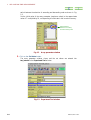
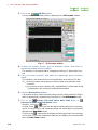
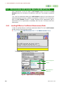
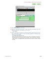
3. Click on the Expmnt button in the Spectrometer Control window.
The Open Experiment window opens.
4. Click on relaxation.
Fig. 1.1 Open Experiment window
5. To perform T1 measurement for 1H, select double_pulse.ex2 from the file
name list box.
To perform T1 measurement for 13 C, select double_pulse_dec.ex2.
The Experiment Tool window used to set the parameters opens.
1-2
NMECA/ECX-USA-3
1 RELAXATION TIME MEASUREMENT
6. Enter the following values.
x_ pulse
tau_interval
relaxation_delay
90° pulse width obtained in Step 2
Value at most 1/10 of the expected T1 as an initial value
Value at least 5 times the expected T1
7. Click on the Submit button.
Measurement is carried out.
8. Perform data processing in the 1D processor window, and adjust the phase
on the phase correction panel in the 1D processor window to turn the peak
downward.
9. Increase tau_interval in the Experiment Tool window, and perform
measurement again.
Perform the phase correction on the obtained spectrum using the same phase
correction values as those obtained in Step 8.
While you repeat this operation, the peak reverses and then turns upward. During
the process, the tau_interval at the time when the peak disappears is obtained. This
is the null point. You can obtain an approximate value of T1 by multiplying the null
point by 1.4.
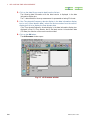
■ Setting the parameters
1. After you obtain the null point, enter the approximate value of T1 multiplied by
10 into relaxation_delay.
The peaks in the spectrum have different T1 values. However, enter 10 times the
maximum T1 value in the peaks used for the T1 measurement.
2. Based on the obtained approximate value of T1, set tau_interval to array
parameter (array variable).
To enter the array parameter for T1 measurement by the inversion recovery method,
be sure to array the values in order from the greatest value. The arrow buttons
NMECA/ECX-USA-3
1-3
1 RELAXATION TIME MEASUREMENT
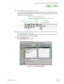
switch between the selection of ascending and descending order as shown in Fig.
1.2.
Set the initial value of the array parameter (maximum value) to the approximate
value of T1 multiplied by 10, corresponding to infinite tau in the inversion recovery.
Switch buttons
between ascending
and descending order
Fig. 1.2
Array parameter window
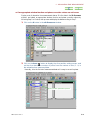
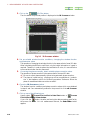
3. Click on the Set Value button.
The array parameter window closes, and the set values are entered into
tau_interval in the Experiment Tool window.
Fig. 1.3
1-4
Experiment Tool window
NMECA/ECX-USA-3
1 RELAXATION TIME MEASUREMENT
1.2
RELAXATION TIME DATA PROCESSING
Data processing following measurement is performed in the nD processor window, and
then T1 calculation is performed in the Curve Analysis window. Chapter 2 explains the
procedure for data processing.
1.2.1
Loading Relaxation Time Measurement Data
First, load measurement data in the nD Processor window in the same way as to perform
2D measurement data processing.
? If
measurement data was transferred from the spectrometer immediately after
relaxation time measurement finished, and the nD Processor window is already
open, you can omit the procedure of Section 1.2.1.
To load relaxation time measurement data (FID) in the nD Processor window,
1. Click on the
Data Processor button in the Delta Console window.
The Open Data for Processing window is displayed.
Version display box
List box
Data information
display box
Fig. 1.4 Open Data for Processing window
NMECA/ECX-USA-3
1-5
1 RELAXATION TIME MEASUREMENT
2. Click on the data file you want to load from the list box.
The following data information with the latest version is displayed in the data
information display box.
The T1 data obtained in the array measurement is represented as having 2D format.
3. If the Time domain/Frequency domain display in the data information display
box is not [s] (time domain data), select the version number from the version
display box so as to display the time domain data.
If the Time domain/Frequency domain display in the data information display box
displayed in Step 2 is Time domain, that is, the latest version is time domain data
(FID data), the selection of the version can be omitted.
4. Click on the Ok button.
The nD Processor window opens.
Fig. 1.5 nD Processor window
1-6
NMECA/ECX-USA-3
1 RELAXATION TIME MEASUREMENT
1.2.2
Processing Relaxation Time Measurement Data
Processing of relaxation time measurement data is performed in the following three
steps.
Step 1
All sets of measurement data from the first to the nth are transformed together under
the same condition.
n
FFT
2
1
Step 2
The processed data sets are transferred to the Curve analysis window. Then, the
peak for T1 calculation is selected from any numbered data set by peak picking.
Step 3
The relaxation times are obtained by approximate calculation.
The procedures are next explained in the order of the above steps.
NMECA/ECX-USA-3
1-7
1 RELAXATION TIME MEASUREMENT
1.2.2a
Fourier-transforming (Step 1)
l If an appropriate window function and phase correction values are already
known and are saved in the processing list
1. Load the desired processing list in the nD Processor window.
Fig. 1.6 nD Processor window
2. Click on either of the
Process File And Put In Data Slate button or
Process File And Put In Data Slate button.
Normally, click on the
button.
button performs the data processing specified in the processing
Clicking on the
list for the first to the nth measurement data sets, and displays the processed data
sets in the Data Slate window.
button performs the data processing specified in the processClicking on the
ing list for the first to the nth measurement data sets, and displays the processed
data sets in the Data Viewer window.
1-8
NMECA/ECX-USA-3
1 RELAXATION TIME MEASUREMENT
l If an appropriate window function and phase correction values are not known
Display a set of relaxation time measurement data as 1D slice data in the 1D Processor
window, and obtain an appropriate window function and phase correction values by
following Step 1 to 6 below; then process and display the data according to Step 7.
1. Click on the X button in the nD Processor window.
Click on one of
above buttons.
2. Click on the Axes
button to display the slice position setting screen, and
set the slice data to the number of points from the number of sets (1 - n) in
the relaxation time measured data.
Normally, slice the first set of measurement data as it is easy to correct its phase.
Slice position parameter input box
NMECA/ECX-USA-3
1-9
1 RELAXATION TIME MEASUREMENT
3. Click on the
1D Slice button.
The slice data at the specified position is displayed in the 1D Processor window.
Fig. 1.7 1D Processor window
4. Change the window function and its parameter values, and enter an
appropriate window function condition.
This operation is the same as that of changing the ordinary 1D data window function.
5. Carry out phase correction, and obtain the appropriate phase correction
values.
This operation is the same as that of correcting the phase of the ordinary 1D data.
• Be sure to perform manual phase correction without using automatic phase
correction.
• If you cannot correct the phase of the J-modulated and J-coupled peak during
T2 measurement, refer to the topic labeled Reference below.
?
6. Close the1D Processor window.
The window function condition and the phase correction values obtained in Steps 4
and 5 are automatically inserted in the processing list in the nD Processor window.
7. Click on the
Process File And Put In Data Slate button or
Process File And Put In Data Viewer button
button.
Normally, click on the
Clicking on the
button performs the data processing specified in the processing list for the first to the nth measurement data sets, and displays the processed
data sets in the Data Slate window.
button performs the data processing specified in the processing
Clicking on the
list for the first to the nth measurement data sets, and displays the processed data
sets in the Data Viewer window.
1-10
NMECA/ECX-USA-3
1 RELAXATION TIME MEASUREMENT
Reference: If you cannot correct the phase of T2 (transverse relaxation
time) measurement data
Repeat Step 4 using the sinbell window function. Perform power processing
without phase correction in Step 5 according to the following procedure:
a. Click on the Append button in the1D Processor window.
b. Select PostTransform—Abs from the menu bar.
The power processing step abs is entered in the processing list.
abs
c. Proceed to Step 6.
NMECA/ECX-USA-3
1-11
1 RELAXATION TIME MEASUREMENT
1.2.2b
Selecting a peak (Step 2)
To perform this operation, the relaxation time measurement data after Fourier
transformation should first be loaded in the Curve Analysis window.
■ To open the Curve Analysis window
u Select Viewers—Analysis—Curve Analysis from the menu bar in the Delta
Console window.
The Curve Analysis window opens.
Fig. 1.8
Curve Analysis window
■ To load relaxation time measurement data after Fourier transformation in
the Curve Analysis window
l If relaxation time measurement data after Fourier transformation is saved on a
hard disk
1. Click on the
Get Data From File button in the Curve Analysis window.
2. Click on the
Open Data File button.
The Open File window opens.
1-12
NMECA/ECX-USA-3
1 RELAXATION TIME MEASUREMENT
Fig. 1.9 Open File window
3. Select the file, in which the relaxation time measurement data after a Fourier
transformation is saved, from the list box in the Open File window, and then
click on the Ok button.
The selected relaxation time measurement data is loaded in the Curve Analysis
window.
Relaxation time measurement data
NMECA/ECX-USA-3
1-13
1 RELAXATION TIME MEASUREMENT
l If relaxation time measurement data after a Fourier transformation is being
displayed
1. Click on the
Open Data By Fingering a Geometry button in the Data
Slate window.
2. Click on the
Open Data File button.
The mouse pointer changes to the shape of a finger.
3. Move the mouse pointer to the area in which the relaxation time measurement data after Fourier transformation is displayed, and click on it.
The selected relaxation time measurement data is loaded in the Curve Analysis
window.
■ To select a peak
Either the Pick mode or the Peak mode is used to select a peak.
If there are a lot of peaks for T1 measurement, and you want to print all those T1 values,
the Peak mode is useful. The peaks to be used in the Peak mode must be listed in the
peak picking list.
The Pick mode can be used to obtain T1 at any position of a spectrum. The top of the
peak is not required for T1 calculation in the Pick mode, making it different from the
Peak mode.
l To select a peak in the Pick mode
1. Click on the Pick button in the Curve Analysis window.
The cursor tool bar in the spectral display area changes to the Pick mode.
1-14
NMECA/ECX-USA-3
1 RELAXATION TIME MEASUREMENT
2. Click on the
Pick position button in the cursor tool Pick mode.
3. Move the mouse pointer onto the X ruler in the spectral display area, and
press and hold the left mouse button.
The cursor is displayed.
4. With the mouse button pressed, move the cursor to the top of the peak
whose relaxation time you want to obtain, and release it.
The pick position marker is displayed at the position at which you released the
mouse button.
l To select a peak in the Peak mode
1. Click on the Peak button in the Curve Analysis window.
2. Click on the
Peak Pick button.
Peak picking is carried out.
If required, before picking peak, change threshold level and noise level so that small
signals or peaks having fine splitting, which T1 value does not need, may not be
picked up.
NMECA/ECX-USA-3
1-15
1 RELAXATION TIME MEASUREMENT
3. Click on the
Select button in the cursor tool Peak mode.
4. Move the mouse pointer onto the X ruler of the spectrum display range, press
and hold down the left mouse button.
The curser appears.
5. Move the cursor to the position which crosses to the top of the peak to obtain
the current relaxation time, and release the mouse button.
A peak position mark appears at the position at which the mouse button was
released.
1-16
NMECA/ECX-USA-3
1 RELAXATION TIME MEASUREMENT
The selected peak values change to yellow, and a peak intensity table is created.
When printing out the T1 values of two or more signals collectively, drag cursor
around the peak area. All peaks listed up by peak picking in the area are selected,
and numerical markers become white.
NMECA/ECX-USA-3
1-17
1 RELAXATION TIME MEASUREMENT
1.2.2c
Obtaining relaxation times by approximate calculation (Step 3)
■ To select an approximate calculation equation
u Select the desired approximate calculation equation in the approximate
calculation equation selection box.
The selected approximate calculation equation is displayed in the approximate
calculation equation display box.
Approximate calculation
equation selection box
Approximate calculation
equation display box
approximate
calculation equation
Description
Weighted Linear
Weighted linear least squares method Lower weights are applied to
measurement points having higher tau_interval values.
Unweighted Linear
Unweighted linear least squares method
Nonlinear
Nonlinear least squares method
? The statement, such as Inv. Recovery, Sat. Recovery, and Spin Lock, which follows
these commands shows experimental method. Inv. Recovery, Sat. Recovery, and
Spin Lock are meaning Inversion Recovery method, Saturation Recovery method,
and Spin Lock method, respectively.
1-18
NMECA/ECX-USA-3
1 RELAXATION TIME MEASUREMENT
■ To execute an approximate calculation and obtain relaxation times
u Click on the Apply button.
The approximate calculation is executed, and the calculated result of the relaxation
time and the yellow approximation curve are displayed.
Calculation results
of relaxation time
Approximation
curve
? When we enter the selection state by pressing the Apply button, the display changes
to Auto. When changing the peak to obtain a relaxation time or when changing
selection of an approximate calculation formula, an approximate calculation is
performed automatically.
NMECA/ECX-USA-3
1-19
1 RELAXATION TIME MEASUREMENT
1.2.3
Plotting Calculation Results
1. Click on the
Plot Data File button in the Curve Analysis window.
Items and buttons for plotting are displayed in the approximation curve display
area.
The Plot Option window opens.
2. Put a check mark on the buttons with the items you want to plot.
To print the T1 values of more than one peak selected in the Peak mode together,
click on the All Slices button.
3. Click on the
Plot data with current state button.
The items that were selected in Step 2 are plotted.
1-20
NMECA/ECX-USA-3
MEASUREMENT OF DIFFUSION
COEFFICIENT AND DATA
PROCESSING
2.1
2.2
2.3
2.4
METHOD OF EVALUATING DIFFUSION COEFFICIENT........................... 2-1
HOW TO MEASURE PFG STRENGTH .......................................................... 2-2
MEASUREMENT OF DIFFUSION COEFFICIENT (D) ................................. 2-4
PROCESSING DIFFUSION MEASUREMENT DATA ................................... 2-8
2.4.1 Loading Diffusion Coefficient Measurement Data .................................... 2-8
2.4.2 Procedure for Processing Diffusion Coefficient Measurement Data ....... 2-10
2.4.2a Fourier transformation (Step 1)......................................................... 2-11
2.4.2b Extraction of peaks, and creation of peak-intensity table (Step 2).... 2-14
2.4.2c Method of obtaining diffusion coefficient by approximate
calculation (Step 3) ........................................................................... 2-21
2.4.3 Plotting Calculation Results ..................................................................... 2-22
NMECA/ECX-USA-3
2 MEASUREMENT OF DIFFUSION COEFFICIENT
2.1
METHOD OF EVALUATING DIFFUSION COEFFICIENT
Generally, diffusion is a process by which the concentration of solution or temperature of
a sample approaches uniformity. However, here “diffusion” means self-diffusion, in
which a molecule changes the position in solution or in solid state. Therefore, the
diffusion coefficient is a measure of transfer of the molecule.
■ Method of evaluating diffusion coefficient by NMR
Although the translational motion of molecule is 3-dimensional motions, the translational
motion actually observed by NMR is only the motion parallel to the z axis because a
magnetic field gradient is applied along the z axis.
If the translational molecular motion is a random walk, the probability of the molecule
moving a distance Δz from its initial position during time t is the following Gaussian
function.
P ( ∆z , t ) = (4πDt ) 1 / 2 exp( − ∆z 2 / 4 Dt )
where D is the diffusion coefficient of the molecule. In this function, the Δz distributes
wide range with increasing t.
In PFG NMR, the transverse magnetization produced by a 90°pulse is in the state
(coherent) where the phase is complete in the beginning. If PFG is applied here, since the
spin receives a magnetic field strength corresponding to its z coordinate, the phase of the
magnetization changes with the magnetic field strength. If the strength of the magnetic
field gradient is G, the duration of the field gradient pulse is δ, and the gyromagnetic
ratio is γ, the final amplitude of phase modulation is Φ = γG∆zδ for a square-wave
field gradient in the direction of z axis. The distribution function of the phase modulation
is as follows.
P (Φ, t ) = (4πDt ) −1 / 2 (γGδ ) −1 / 2 exp( −Φ 2 / 4(γGδ ) 2 Dt )
Therefore, when the coherence is reestablished due to rephasing by a second PFG after
vanishing due to dephasing by the first PFG, the signal intensity is as follows if the time
between the two FG pulses is Δ：
I (G, ∆ ) = I (0, ∆ ) exp( − D(γGδ ) 2 ∆ )
Furthermore, when the influence of the diffusion between FG pulses cannot be
disregarded, it is corrected as follows.
I (G, ∆ ) = I (0, ∆ ) exp( − D(γGδ ) 2 ( ∆ − δ / 3))
Therefore, the diffusion coefficient D can be evaluated from the formula by changing
either the strength of the magnetic field gradient G, the duration of the field gradient
pulse δ, or the time between the two magnetic-field-gradient pulses Δ.
NMECA/ECX-USA-3
2-1
2 MEASUREMENT OF DIFFUSION COEFFICIENT
2.2
HOW TO MEASURE PFG STRENGTH
In order to obtain the diffusion coefficient, it is necessary to measure the strength of
magnetic-field gradient G. Therefore, the maximum magnetic-field-gradient strength of
the system being used should be measured before carrying out an actual measurement.
■ Simple way to measure PFG strength
1. Prepare a water sample with the liquid height adjusted to about 5 mm.
? A sample tube such as a micro-cell, in which the height of liquid is clearly
known, is needed.
2. Click on the Expmnt button in the Spectrometer Control window.
The Open Experiment window opens.
3. Click on diffusion.
Fig. 2.1 Open Experiment window
4. Select the fg_power_check.ex2 sequence from the File name list box.
The Experiment Tool window for setting parameters opens.
5. Set the parameter grad_amp.
? Since
a long magnetic-field-gradient pulse will be used in the
fg_power_check.ex2 sequence, do not use a large magnetic-field gradient. Use
a value of 1% to 5% for the value of grad_amp.
6. Click on the Submit button.
A measurement is performed.
7. Process the data in the 1D processor window and display the absolute value
of the spectrum.
In order to display the absolute value, perform abs processing.
8. Measure the frequency at the both ends of the obtained rectangular spectrum
in Hz.
2-2
NMECA/ECX-USA-3
2 MEASUREMENT OF DIFFUSION COEFFICIENT
9. Select Tools—Math—Gradient Strength from the menu bar of the Delta
Console window.
The Gradient Strength window opens.
10. Input value into each item of the Gradient Strength window.
Select 1H (Proton) in Nucleus, and input the liquid height of the sample used into
Coil length column. Moreover, input the frequency obtained in step 8 into the Left
position and Right position column.
The obtained magnetic-field-gradient strength is displayed on Gradient Strength
window.
NMECA/ECX-USA-3
2-3
2 MEASUREMENT OF DIFFUSION COEFFICIENT
2.3
MEASUREMENT OF DIFFUSION COEFFICIENT (D)
As discussed above, the measurement of the diffusion coefficient can be carried out by
changing either the field-gradient strength G, the duration of gradient pulse δ, or the
time between two FG pulses Δ.
However, in the measurement in which a time parameter such as the duration of the field
gradient pulse δ or time between FG pulses Δ changes, you have to take into account
the influences time, such as relaxation. Therefore, the measurement by changing
magnetic-field-gradient strength G is presently in general use. The procedure for
measurement of the diffusion coefficient by changing the magnetic-field-gradient
strength G is explained below.
■ To obtain measurement conditions
1. Stop the sample spinning, and tune the probe.
2. Check the 90° pulse width.
? In order to improve the accuracy of the diffusion coefficient measurement, we
recommend that you check the 90° pulse width of the sample you are measuring. For checking the 90° pulse, perform an array measurement using the
measurement mode single_pulse.ex2 or single_pulse_dec.ex2.
3. Click on the Expmnt button in the Spectrometer Control window.
The Open Experiment window opens.
4. Click on diffusion.
5. Select the desired sequence from the File name list.
The Experiment Tool window for setting up parameters opens.
6. Input the following value if needed.
The values of x_pulse and gradient_max of the following are recalled automatically from the default values in the probe file. Input values when values obtained in
step 2 differ from the values in the probe file.
2-4
NMECA/ECX-USA-3
2 MEASUREMENT OF DIFFUSION COEFFICIENT
x_pulse:
gradient_max:
?
90°pulse width which you obtained in step 2.
The maximum magnetic field strength [T/m] in the
system currently used.
For the maximum magnetic field strength, input into gradient_max, measure
the value for every system combination of the probe and the maximum output
of the FG power supply referring to section 2.2 "How to measure PFG
strength".
7. Input values for the parameters of measurement of the diffusion coefficient.
The following three parameters are necessary for measuring the diffusion coefficient.
Interval of two FG pulses (diffusion time Δ).
diffusion_time:
Duration of magnetic-field-gradient pulse.
grad_1:
Magnetic-field strength (G).
grad_1_amp:
The duration of magnetic-field-gradient pulse (δ) which is used for calculation
of the diffusion coefficient is not equivalent to the parameter grad_1 in some
sequences. Refer to the parameter delta for the duration of the magnetic-field-gradient pulse (δ) used for the calculation of the diffusion coefficient.
?
Fig. 2.2
Experiment Tool window
8. Input a number about 10 times the value of T1 into relaxation_delay.
9. Perform an array measurement at the minimum value and maximum of the
variable magnetic-field strength that are used in the actual measurement.
For example, to change magnetic field gradient from 3 mT/m to 0.27 T/m, carry out
an array measurement at 3 mT/m and 0.27 T/m.
The instrument cannot output a magnetic field strength greater than gradient_max.
?
NMECA/ECX-USA-3
2-5
2 MEASUREMENT OF DIFFUSION COEFFICIENT
Fig. 2.3
Array parameter window
10. Process the data in the nD processor window, and check the decay of the signal.
Repeat steps 8 and 9, changing the values of diffusion_time and grad_1 so that the
decay ratio of the signal may become in the range of 10:1 to 20:1 for the maximum
and minimum of field gradient strength.
■ Measurement of diffusion time
1. Stop sample spinning, and adjust tuning of the probe.
2. Check the 90°pulse width.
? In order to improve the accuracy of the diffusion coefficient measurement, we
recommend you to check the 90° pulse width of the sample to measure. To
check the 90° pulse, perform an array measurement in the single_pulse.ex2 or
single_pulse_dec.ex2 measurement mode.
3. Set up the various parameters obtained in the procedure "■ To obtain
measurement conditions”.
Set up scans so that you obtain a sufficient S/N ratio also for the decay signal.
?
2-6
NMECA/ECX-USA-3
2 MEASUREMENT OF DIFFUSION COEFFICIENT
4. Set grad_1_amp to a suitable array variable in the range of the minimum
and minimum value of the variable magnetic-field gradient used in the
condition setting.
In measurement of a diffusion coefficient, good measurement can be performed
changing an array variable so that the 2nd power of the magnetic field gradient
may be measured at equal intervals. For this reason, the array variable can be
easily set by selecting Logarithmic as an Array Type and by setting the Base
value to 2.
?
5. Click on the Set Value button.
Close the array parameter window, and input the set values into the Experiment
Tool window.
6. Click on the Submit button.
Measurement starts.
NMECA/ECX-USA-3
2-7
2 MEASUREMENT OF DIFFUSION COEFFICIENT
2.4
PROCESSING DIFFUSION MEASUREMENT DATA
After measurement, process the data in nD Processor window, and use the Curve
Analysis window for calculation of the diffusion coefficient. The procedure is explained
below.
First, recall the measurement data into the nD Processor window as in two-dimensional
measurement data processing. In addition, the operation of section 2.4.1 is not necessary
when the nD Processor window is already displayed when measurement data is
transmitted from the spectrometer immediately after the end of diffusion-coefficient
measurement.
2.4.1
Loading Diffusion Coefficient Measurement Data
In order to load the diffusion coefficient measurement data (FID) into the nD Processor
window, perform the following procedure.
1. Click on the
Data Processor button in the Delta Console window.
The Open Data for Processing window appears.
Version display box
List box
Data information
display box
Fig. 2.4 Open Data for Processing window
2-8
NMECA/ECX-USA-3
2 MEASUREMENT OF DIFFUSION COEFFICIENT
2. Click the data file in the filename list box.
In the data information display box, the data information of the newest version is
displayed as shown below. Note that the format of the data obtained by the array
measurement is displayed as 2D.
Time domain / Frequency domain (unit)
s:
Time domain data (FID data)
Hz, PPM: Frequency domain data (Fourier transformed data)
T:
Field intensity
1D/2D/nD
A number of data points
Row of data
R: Ranged
S: Sparsed
Revision_time
Comment
Creation_time
3. Looking at the data information display box, and select the version of stored
FID from the version display box.
If the newest version of the data displayed in step 2 is the time domain data (FID
data), selection of a version is unnecessary.
4. Click on the Ok button.
The nD Processor window opens.
Fig. 2.5 nD Processor window
NMECA/ECX-USA-3
2-9
2 MEASUREMENT OF DIFFUSION COEFFICIENT
2.4.2
Procedure for Processing Diffusion Coefficient
Measurement Data
The processing of the diffusion coefficient measurement data consists of the following
three steps.
Step 1
Fourier-transform the diffusion measurement data sets under the same conditions
for the 1 to n-th measurement data set as shown in the following schematic figure.
n
FFT
2
1
Step 2
Transmit the processed data to the Curve Analysis window. Then, select the peaks
to use to perform the diffusion coefficient calculation by picking the peaks.
Step 3
Obtain the diffusion coefficient using the approximate calculation.
The procedure is explained in the order of these step.
2-10
NMECA/ECX-USA-3
2 MEASUREMENT OF DIFFUSION COEFFICIENT
2.4.2a
Fourier transformation (Step 1)
Displaying one diffusion coefficient measurement data set in the 1D Processor window as
1-dimensional slice data, search a suitable window function and phase correction value.
1. Click on the X button in the nD Processor window.
Click on one of
above buttons.
2. Click on the Axes
button to display the slice position setting screen, and
set the slice data to the number of points from the number of sets (1 - n) in
the diffusion coefficient measurement data.
Usually, slice the first measurement data, whose phase correction is easy to carry
out easily.
Slice position
parameter input box
NMECA/ECX-USA-3
2-11
2 MEASUREMENT OF DIFFUSION COEFFICIENT
3. Click on the
1 D Slice button.
The slice data at the specified position is displayed on the 1D Processor window.
Fig. 2.6
1D Processor window
4. Set up suitable window function conditions, changing the window function
and parameter value.
The operation of changing the window function is the same as that of usual 1D data.
When calculating the diffusion coefficient, only the height information of a peak is
required. Therefore, in order to reduce the contribution of noise, it is more effective
to use a wider window function than usual.
5. Correcting the phase manually, obtain suitable phase-correction value.
The operation of phase correction is the same as that of the usual 1D data.
? Be sure to correct phase manually without using automatic phase correction.
? The phase of a peak having J coupling may not be corrected due to J modula-
tion. If that happens, refer to the following procedure "Reference: When the
phase of measurement data can not be corrected."
6. Close the 1D Processor window.
The window function conditions and phase-correction values which were obtained
in steps 4 and 5 are automatically entered in the process list of the nD Processor
window.
7. Click on one of the following icon.
Usually select
Process File And Put In Data Slate button or
Process
File And Put In Data Viewer button.
If you click the
button, the after performing the data processing specified by
the process list to the 1 to n-th measurement data set, the Data Slate window
appears.
2-12
NMECA/ECX-USA-3
2 MEASUREMENT OF DIFFUSION COEFFICIENT
If you click the
button, the after performing the data processing specified the
process list to the 1 to n-th measurement data sets, the Data Viewer window appears.
l Reference: When the phase of measurement data cannot be corrected
Power processing replaces phase correction in step 5.
Perform the following operational procedure.
a. Click on the
Append button in the 1D Processor window.
b. Select Post Transform—Abs in the menu bar.
The abs function for power processing is entered into the process list.
abs
c. Go to step 6.
NMECA/ECX-USA-3
2-13
2 MEASUREMENT OF DIFFUSION COEFFICIENT
2.4.2b
Extraction of peaks, and creation of peak-intensity table (Step 2)
This operation calls the diffusion coefficient measurement data that performed Fourier
transform processing to the Curve Analysis window, and change the Mode to Diffusion
Analysis.
■ Open the Curve Analysis window and change the Mode
1. Select Viewers—Analysis—Curve Analysis in the menu bar of for Delta
Console window.
The Curve Analysis window opens.
Fig. 2.7
Curve Analysis window
2. Change the Mode to Diffusion Analysis.
The window changes to the Diffusion Analysis mode.
Mode
2-14
NMECA/ECX-USA-3
2 MEASUREMENT OF DIFFUSION COEFFICIENT
■ Reading the data Fourier transformed in the Curve Analysis window
l When Fourier transformated diffusion coefficient measurement data is saved on
the hard disk
1. Click on the
Get Data From File button in the Curve Analysis window.
2. Click on the
Open Data File button.
The Open File window opens.
Fig. 2.8 Open File window
3. Select the file containing the Fourier transformed diffusion coefficient
measurement data from the list box of in the Open File window, and click on
the Ok button.
The selected diffusion coefficient measurement data is loaded into the Curve
Analysis window.
NMECA/ECX-USA-3
2-15
2 MEASUREMENT OF DIFFUSION COEFFICIENT
l When Fourier-transformed diffusion coefficient measurement data is displayed
1. Click on the
Open Data By Fingering a Geometry button in the Data
Slate window.
2. Click on the
Open Data File button.
The mouse pointer changes to the shape of a finger.
3. Move the mouse pointer to the area where the Fourier-transformed diffusion
coefficient measurement data is displayed, and click it.
The selected diffusion coefficient measurement data is recalled into the Curve
Analysis window.
■ For extracting peak
There are two methods of extracting method of a peak Pick mode and Peak mode.
If you are using a large number of peaks to calculate the diffusion coefficient, then when
printing those diffusion coefficient values collectively, the Peak mode is convenient. The
candidate peaks of the Peak mode should be listed by peak picking beforehand.
Using the Pick mode, yuo can measure the diffusion coefficient of an arbitrary peak in a
spectrum. It differs from the Peak mode, and it is not necessary that the point for
calculating the diffusion coefficient is the top of the peak.
l Method of extracting in Pick mode
When extracting the peaks in the Pick mode, the procedure for creating the
peak-intensity table is as explained below.
1. Click on the Pick button in the Curve Analysis window.
The cursor tool in the spectrum display range changes to the Pick mode.
2-16
NMECA/ECX-USA-3
2 MEASUREMENT OF DIFFUSION COEFFICIENT
2. Select the Pick—Pick position by cursor tool.
3. Move the mouse pointer onto the X ruler in the spectrum display area, and
press and hold down the left mouse button.
A cursor appears.
4. While continuing to hold down the left mouse button, move the cursor so that
it intersects the top of a peak that you want to use to calculate the diffusion
coefficient; then release the mouse button.
A pick position marker is displayed at the position where you released the mouse
button.
5. When displaying the peak-intensity table, select File—Point List… in the pull
down menu of the Curve Analysis Tool.
NMECA/ECX-USA-3
2-17
2 MEASUREMENT OF DIFFUSION COEFFICIENT
The Points List appears.
l Method of extracting Peak in Peak mode
In the Peak mode, the procedure for extraction of a peak and creation of a peak-intensity
table is as explained below.
1. Click on the Peak button in the Curve Analysis window.
2. Click on the
Peak Pick Data button.
A peak pick is performed.
If necessary, before performing peak picking, adjust the threshold and noise level so
that small signals and fine splitting of the peak, which you do not need to obtain the
diffusion coefficient, may not be picked.
2-18
NMECA/ECX-USA-3
2 MEASUREMENT OF DIFFUSION COEFFICIENT
3. Select Peak—Select by cursor tool.
4. Move the mouse pointer onto the X ruler in the spectrum display area, and
press and hole down the left button of the mouse.
Cursor appears.
5. While continuing to hold down the left mouse button, move the cursor to the
top of a peak that you want to use to calculate the diffusion coefficient; then
release the mouse button.
The selected peak changes to white.
When printing the diffusion coefficient value of two or more peaks collectively,
drag the mouse cursor around the area of the peaks. All the peaks listed in the peakintensity table in the dragged area are selected, and their numerical markers change
to white.
NMECA/ECX-USA-3
2-19
2 MEASUREMENT OF DIFFUSION COEFFICIENT
6. When displaying the peak-intensity table, select File—Point List… in the pull
down menu of the Curve Analysis Tool.
The Point list appears
2-20
NMECA/ECX-USA-3
2 MEASUREMENT OF DIFFUSION COEFFICIENT
2.4.2c
Method of obtaining diffusion coefficient by approximate calculation
(Step 3)
This method calculates the diffusion coefficient approximately.
■ Input parameters used for measurement
u Select the parameters used as variables for the array measurement in the Y
Value Type check boxes.
Enter a check mark into the check box of a variable to selected it.
u Input the gyromagnetic ratio of the nucleus used for calculation and the other
parameters which were not used as array variables into the parameter input
boxes.
When the following parameters are used in the used sequence, these default values
are read.
γ:
G:
δ:
Δ:
x_domain: Gyromagnetic ratio of an observed nucleus
grad_1_amp : Amplitude of magnetic-field-gradient pulse
delta: Duration of magnetic-field-gradient pulse
diffusion_time: Diffusion time
■ To obtain diffusion coefficient by approximate calculation
u
Click on the Apply button.
An approximate calculation is performed, and the result of the calculation of a
diffusion coefficient and the approximation curve in yellow appear.
? When entering in the selection state by pressing the Apply button, the display
changes to Auto. When changing the peak which obtains the diffusion coefficient,
or when changing the parameter value, an approximate calculation is performed
automatically.
NMECA/ECX-USA-3
2-21
2 MEASUREMENT OF DIFFUSION COEFFICIENT
2.4.3
Plotting Calculation Results
1. Click on the
Plot Data File button in the Curve Analysis window.
The Plot Option window opens.
2. Place a check mark in the box of each item that you want to plot.
When two or more peaks are selected in the Peak mode and you wont to print the
diffusion coefficient values of those peaks collectively, turn on All Slices.
In order to put check mark on an item to plot, click its button from Curves &
Info, Peaks & Equations or Vectors & Equations, or the check button of an
item to plot directly.
?
3. Click on the
Plot data with current state icon.
The items selected in step 2 are plotted.
2-22
NMECA/ECX-USA-3
DOSY MEASUREMENT AND
DATA PROCESSING
3.1
3.2
3.3
OUTLINE OF DOSY......................................................................................... 3-1
DOSY MEASUREMENT .................................................................................. 3-2
PROCESSING DOSY DATA............................................................................. 3-7
3.3.1 Reading DOSY Measurement Data............................................................ 3-7
3.3.2 Procedure for Processing DOSY Measurement Data................................. 3-9
3.3.2a Processing for x-axis of DOSY measurement data (Step 1) ............. 3-10
3.3.2b Processing for y-axis of DOSY measurement data (Step 2) ............. 3-12
NMECA/ECX-USA-3
3 DOSY MEASUREMENT
3.1
OUTLINE OF DOSY
The DOSY (Diffusion-Ordered NMR SpectroscopY) method evolves the diffusion
coefficient of a sample on one axis in the two-dimensional spectrum by inverse Laplace
transformation or curve fillings.
■ Principle of DOSY
As described in Chapter 2 “Measurement of Diffusion Coefficient and Data Processing",
when the phase coherence of the spin is lost due to the first FG pulse and the phase
coherence is restored by a second FG pulse, the signal intensity is as follows if interval
of two FG pulses is Δ.
I (G, ∆ ) = I (0, ∆ ) exp( − D(γGδ ) 2 ( ∆ − δ / 3))
Therefore, when two or more NMR signals overlap in the same chemical shift, since the
echo intensity becomes a linear combination of the signals, the echo is given as follows.
N
I (G, ∆ ) = å I j (0, ∆ ) exp( − D j (γGδ ) 2 ( ∆ − δ / 3))
(3.1)
j=I
Moreover, for a sample which has a continuous molecular weight distribution like a
polymer, the echo intensity is given as follows.
∞
I (G, ∆ ) = ò G( D ) exp(− D(γGδ ) 2 ( ∆ − δ / 3))dD
(3.2)
0
where G (D) is the distribution function of D.
Such overlapping signals evolve along with one axis by the diffusion coefficient using
the peak intensity. Curve fitting is used for a signal like equation (3.1) and inverse
Laplace transformation is used for a signal like equation (3.2).
NMECA/ECX-USA-3
3-1
3 DOSY MEASUREMENT
3.2
DOSY MEASUREMENT
A DOSY measurement is basically the same as the diffusion coefficient measurement
discussed in previous chapter. The only difference between DOSY and diffusion
coefficient measurement is that the target of measurement is a multicomponent system or
a system having a distribution of molecular weight.
■ To obtain measurement conditions
1. Measure the maximum magnetic-field-gradient intensity of PFG (FG pulse)
used measurement.
Refer to Section 2.2 "How to measure PFG strength." for measuring FG pulse
strength.
?
2. Stop the sample spinning, and tune the probe.
3. Check the 90° pulse width.
? In order to improve the accuracy of a diffusion coefficient measurement, we
recommend you to check 90° pulse width of the sample to measure. In order
to check 90° pulse, perform an array measurement using the measurement
mode of single_pulse.ex2 or single_pulse_dec.ex2.
4. Click on the Expmnt button in the Spectrometer Control window.
The Open Experiment window opens.
5. Click on diffusion.
6. Select a sequence to use from the File name list box.
The Experiment Tool window for setting parameters opens.
7. Input the following values if needed.
For the values of x_pulse and gradient_max shown in below, the default value in
the probe file is automatically called. Input value when the values you found in step
3 differs from the value in the probe file.
90° pulse width which you obtained in step 3.
x_pulse:
3-2
NMECA/ECX-USA-3
3 DOSY MEASUREMENT
gradient_max:
The maximum applicable magnetic field strength in the
system currently used in [T/m].
? For the maximum magnetic field strength to input into gradient_max, measure
the value for every different combination of the probe and the maximum output
of the FG power supply, referring to section 2.2 "How to measure PFG
strength".
8. Input values for the parameter of measurement of the diffusion coefficient.
The following three parameters are necessary for measuring the diffusion coefficient
diffusion_time:
grad_1 :
grad_1_amp:
Time interval of two FG pulses (diffusion time Δ)
Duration of magnetic-field-gradient pulse
Magnetic-field-gradient strength (G) [T/m]
? The duration of magnetic-field-gradient pulse (δ) for DOSY processing is not
equivalent to the parameter grad_1 in some types of sequence. DOSY processing of Delta program refers to parameter delta automatically for duration of
the magnetic-field-gradient pulse (δ).
Fig.3.1
Experiment Tool window
9. Input about 10 times the value of T1 into relaxation_delay.
10. Perform an array measurement at the minimum and maximum value of the
variable magnetic-field-gradient strength which are used in the actual
measurement.
For example, when changing magnetic field from 3 mT/m to 0.27 T/m, perform an
array measurement at 3 mT/m and 0.27 T/m.
A magnetic field strength greater than gradient_max cannot be output.
?
NMECA/ECX-USA-3
3-3
3 DOSY MEASUREMENT
Fig. 3.2
Array parameter window
11. Process the data in the nD processor window, and check the decay of the
signal.
Be careful of the following points when two or more kinds of molecules are included.
• When the maximum magnetic field gradient to use is applied, adjust measurement
conditions so that a signal can be observed also for the molecule with the largest
diffusion coefficient.
• Also for the molecule with the smallest diffusion coefficient, select the measurement conditions to make at the decay of the signal intensity about 1/2.
When the measurement sample includes molecules whose the diffusion
coefficients different largely, suitable decaying data may not be obtained for
each kind of molecule. In this case, we recommend that you divide the measurement sample into a group having a large diffusion coefficient and a group
having a small diffusion coefficient, and measure two times under conditions
suitable for each group separately.
?
3-4
NMECA/ECX-USA-3
3 DOSY MEASUREMENT
■ DOSY measurement
1. Stop sample spinning, and tune the probe.
2. Check the 90° pulse width.
? In order to improve the accuracy of diffusion coefficient measurement, we
recommend that you check the 90° pulse width of the measurement sample. In
order to check the 90° pulse, perform an array measurement using the measurement mode of single_pulse.ex2 or single_pulse_dec.ex2.
3. Input various parameters obtained by the above procedure “To obtain
measurement conditions”.
Set scans so that sufficient signal to noise ratio can be obtained for every
molecule groups.
?
4. Set grad_1_amp to suitable array variable in the range of the minimum and
maximum values of the variable magnetic-field-gradient which were used in
condition setting.
5. Click on the Set Value button.
Close the array parameter window, and input the settings into Experiment Tool
window.
NMECA/ECX-USA-3
3-5
3 DOSY MEASUREMENT
6. Click on the Submit button.
Measurement starts.
3-6
NMECA/ECX-USA-3
3 DOSY MEASUREMENT
3.3
PROCESSING DOSY DATA
After measurement process the data in the nD Processor window.
First, measurement data are loaded into the nD Processor window as in two-dimensional
measurement data processing. In addition, when the measurement data is transmitted
from the spectrometer immediately after the end of DOSY measurement and the nD
Processor window is already open, the operation of section 3.3.1 is not necessary.
3.3.1
Reading DOSY Measurement Data
In order to load the data (FID) of DOSY measurement into the nD Processor window,
perform the following procedure.
1. Click on the
Data Processor button in the Delta Console window.
The Open Data for Processing window appears.
Version display box
List box
Data information
display box
Fig. 3.3 Open Data for Processing window
2. Click the data file called from the list box.
The data information on the newest version is displayed in the data information
display box as shown below. Note that the format of the data obtained by the array
measurement is displayed as 2D data.
NMECA/ECX-USA-3
3-7
3 DOSY MEASUREMENT
Time domain / Frequency domain (unit)
s:
Time domain data (FID data)
Hz, PPM:
Frequency domain data (Fourier transformed data)
T:
Field intensity
1D/2D/nD
A number of data points
Row of data
R: Ranged
S: Sparsed
Revision_time
Comment
Creation_time
3. Looking at the data domain of the data information display box, and select
the version of stored FID from the version display box.
If the newest version of the data displayed in step 2 is the time domain data,
selection of the version is unnecessary.
4. Click on the Ok button.
nD Processor window opens.
Fig. 3.4 nD Processor window
3-8
NMECA/ECX-USA-3
3 DOSY MEASUREMENT
3.3.2
Procedure for Processing DOSY Measurement Data
The processing of the DOSY measurement data consists of the following two steps.
Step 1
Fourier transformation the X-axis of DOSY measurement data set under same
conditions for the 1 to n-th measurement data set as shown in the following schematic diagram.
n
FFT
2
1
1
2
n
ILT
D [um2/s]
Step 2
For the processing of the Y-axis of DOSY measurement data, Inverse Laplace
Transformation is carried out on every data point that is Fourier transformed along
the X-axis as shown in the following schematic diagram.
[ppm]
The procedures are explained in the order of these steps below.
NMECA/ECX-USA-3
3-9
3 DOSY MEASUREMENT
3.3.2a
Processing for x-axis of DOSY measurement data (Step 1)
Display one data of DOSY measurement data in the 1D Processor window as 1D slice
data, and search a suitable window function and phase correction values.
1. Click on the X button in the nD Processor window.
Click on one of
above buttons.
2. Click on the Axes
button to display the slice position setting screen, and
set the slice data to the number of points from the number of sets (1 - n) in
the DOSY measurement data.
Usually, slice the first measurement data whose phase correction is easy to performed.
Slice position
parameter input box
3-10
NMECA/ECX-USA-3
3 DOSY MEASUREMENT
3. Click on the
1D Slice button.
The slice data at the specified position is displayed in the 1D Processor window.
Fig.3.5
1D Processor window
4. Changing the window function and parameter value, set up suitable window
function conditions.
The operation of changing the window function is the same as that of usual 1D data.
The height information of a peak is required for inverse Laplace transformation of
DOSY. Therefore, in order to reduce the contribution of noise, it is more effective
to use a larger window function conditions than usual data processing.
5. Correct a phase manually, and obtain suitable phase correction values.
The phase correction is the same as that of the usual 1D data.
? Be sure to perform phase correction manually without using automatic phase
correction.
? A phase may not correct at the peak having J coupling due to J modulation. If
that happens, refer to section 2.4.2 "Reference: When the phase of measurement data can not be corrected."
6. Close the 1D Processor window.
The window function conditions and phase correction value, which were obtained
in steps 4 and 5, are automatically entered in the process list in the nD Processor
window.
7. Select Post Transform—Math—Real from the menu bar.
Real processing is sentered in the process list of windows.
In inverse Laplace transformation processing of DOSY, only real data is need.
?
NMECA/ECX-USA-3
3-11
3 DOSY MEASUREMENT
3.3.2b
Processing for y-axis of DOSY measurement data (Step 2)
Carry out inverse Laplace transformation of the Y-axis for the data Fourier transformed
in the direction of the X-axis in step 1.
1. Click on the Y button in the nD Processor window.
Click on one of
above buttons.
2. Select Transform—DOSY in the menu bar, and select the algorithm used for
processing.
3. Set up the various parameters.
There are the following parameters.
In the nD Processor window, only three parameters are displayed simultaneously. When the parameters you want to change are not displayed, display them
by clicking the
Back to previous parameter group button or the
Advance to next parameter group button.
?
Start:
Stop:
Interp:
This is the minimum value of the range over which to search for the
peak to use to measure the diffusion coefficient.
This is the maximum value of the range over which to search for the
peak to use to measure the diffusion coefficient.
This determines the number of points to interpolate in the diffusion
coefficient axis (Y-axis ).
Example: When the number of data points is three, and Interp is 2,
thenumber of points becomes 7 after processing.
Original points
Interpolated points
? In the CONTIN method, values of Interp that are 15 or more are
suitable.
3-12
NMECA/ECX-USA-3
3 DOSY MEASUREMENT
Threshold:
Species:
Peaks:
Ratio:
Threshold level of the peak to used for processing.
When Threshold is 0, the default value of Delta
software is used.
Set the total number of components expected.
Set this to the maximum number of the diffusion coefficient expected
for each chemical shift.
In the L-Marquardt method, set Peaks to 1.
In the SPLMOD method, set this to the minimum ratio of the
different diffusion coefficients having equal chemical shift.
This parameter applies only to the SPLMOD
method.
Set this to the permissible error in the SPLMOD method as decimal.
Example: When Error is 0.2, the permissible error is 20%.
this parameter applies only to the SPLMOD method.
Set this to the gyromagnetic ratio of the nucleus used for processing.
?
?
?
Error:
Gamma:
?
4. Click on the Process File And Put In Data Viewer button.
Data processing is performed, and DOSY data is displayed.
5. Repeating steps 3 and 4, obtain the search condition for the diffusion
coefficient in the suitable range.
l Logarithmic display of diffusion coefficient axis.
In the diffusion coefficient axis, logarithmic display may be more legible. Here, the
procedure for logarithmic display is explained.
1. Set cursor tool to Select geometry in Select mode, and click on DOSY data
display area on the screen.
The DOSY data display range is selected.
2. Right click in the data display area.
A pop-up menu appears.
NMECA/ECX-USA-3
3-13
3 DOSY MEASUREMENT
3. Select the bases of the logarithm from Logarithm Base—Y Ruler of the
pop-up menu.
The base can be selected from 2 and 10 for common logarithms, and e for natural
logarithm.
4. Right click in the data display area again.
A pop-up menu appears.
5. Select Options—Ruler—Logarithmic Y Ruler from the pop-up menu.
The Y-axis changes to logarithmic display.
3-14
NMECA/ECX-USA-3
MEASUREMENT OF SR-MAS
OUTLINE OF SR-MAS MEASUREMENT ...................................................... 4-1
HOW TO ADJUST MAGIC ANGLE................................................................ 4-2
ADJUSTMENT OF RESOLUTION .................................................................. 4-4
ADJUSTING TUNING...................................................................................... 4-6
4.4.1 When Tuning is Necessary......................................................................... 4-6
4.4.2 How to Tune............................................................................................... 4-6
4.4.3 How to Adjust Tuning Precisely for Carbon13........................................ 4-10
4.5 TEMPERATURE CONTROL.......................................................................... 4-11
4.6 SPINNING SPEED AND RESOLUTION....................................................... 4-12
4.1
4.2
4.3
4.4
NMECA/ECX-USA-3
4 MEASUREMENT OF SR-MAS
4.1
OUTLINE OF SR-MAS MEASUREMENT
SR-MAS（Swollen Resin Magic Angle Spinning）is a measurement method for gel
samples, swollen resin of solid phase synthesis, and heterogeneous systems such as tissue.
In order to perform this measurement, it is necessary to use the special SR-MAS probe
which can carry out MAS measurement and the special-purpose sample tube use for
liquid samples which does not leak even if it rotates at several kilohertz.
to the manual of the SR-MAS for the preparation and the operation of the
F Refer
SR-MAS probe.
The pulse sequence used for a SR-MAS measurement is the same sequence as the pulse
sequence used for general solution NMR measurement. Therefore, the basic measuring
method and data-processing method are the same as those of solution NMR.
? However, the pulse sequence using field gradient (FG) cannot be used.
Here, the method of adjustment of the magic angle, the resolution and tuning, the
temperature controlling, and the relationship between spinning speed and resolution, that
is peculiar to the SR-MAS NMR measurement and different from the general solution
NMR measurement in the spectrometer, are explained.
■ SR-MAS measurement
SR-MAS is the abbreviation of Swollen Resin Magic Angle Spinning. It means that the
resin swallenby the solvent is directly measured under the condition of several-kilohertz
MAS spinning. The resolution of the spectrum of semisolids (soft solid) and
high-viscosity liquids will be improved by reducing the residual weak dipole-dipole
interaction of a sample by MAS. Moreover, higher resolution can be reached by
averaging inhomogeneity of the local magnetic field around the rotating axis.
—— CAUTION ———————
Be sure to rotate a sample in SR-MAS experiment. If you measure
without the air for sample spinning flowing, the probe may be damaged.
However, when you carry out the resolution adjustment using single_pulse.ex2, damage to the probe does not occur even if a measurement is carried out without air flowing.
NMECA/ECX-USA-3
4-1
4 MEASUREMENT OF SR-MAS
4.2
HOW TO ADJUST MAGIC ANGLE
—— CAUTION ———————
Receive instruction from an experienced person when the magic angle
is adjusted the first time. The SR-MAS probe may be damaged if unsuitable adjustment is performed.
1. Insert the reference sample KBr.
2. Start the spinning.
3. Insert the stick for magic-angle adjustment through the top of the SCM.
4. Change LF (Lower frequency) channel to Bromine79 observation.
Check the combination of the stick and the tuning dial for Bromine79 observation.
5. Load the pulse sequence global/experiments/single_pulse.ex2 in the
Experiment Tool window, and perform the following setting.
• Set observed nucleus to Bromine79.
• Set x_sweep to 1000 ppm.
• Add the repeat flag to Header, and turn on spinning.
• Set scans to 1.
6. Click on the Submit button.
The pulse occurs, and measurement starts.
If the Inform window appears, click on the GO button.
?
7. Adjusts a phase by the following procedure.
a. Click on the View button.
The View Tool window opens.
b. After clicking on the View button, click on the Process vector button to
change the display.
c. Select Processing—Phase and Processing—Phase Boxes.
The Phase Boxes window opens.
d. Adjust the phase.
8. Adjust the magic angle.
Turn the adjustment stick to maximize the spinning side band of KBr (Fig. 4.1) .
The gear of the magic-angle adjustment mechanism has some backlash.
Therefore, adjust it by turning the dial for fine-tuning in only one direction.
?
FT
Fig 4.1 Free Induction Decay (left) and spectrum (right)
after magic-angle adjustment
4-2
NMECA/ECX-USA-3
4 MEASUREMENT OF SR-MAS
9. After completing magic-angle adjustment, select the current measurement in
the Spectrometer Control window, and click on the STOP button.
If a measurement is stopped while it is in progress, the data file is stored
automatically, and the version of the data file increases. In order to keep space
free on the hard disk, delete the file at any time.
?
10. Remove the stick for adjustment.
? Adjustment of the magic angle may change the resolution. Be sure to check the
resolution according to section 4.3 "Adjustment of resolution", and adjust the shim
values if needed.
NMECA/ECX-USA-3
4-3
4 MEASUREMENT OF SR-MAS
4.3
ADJUSTMENT OF RESOLUTION
1. Insert the chloroform (CHCl3)sample.
It is not necessary to perform spinning.
2. Select Config—Shim on FID in the pull down menu of the Spectrometer
Control window.
3. Click on the Start button.
The spectrum is updated continuously.
4. Adjust the phase.
5. Expand near the peak, and check the resolution.
4-4
NMECA/ECX-USA-3
4 MEASUREMENT OF SR-MAS
Fig. 4.2 View Tool window in resolution adjustment
6. If the resolution is not good, adjust the resolution as followings
a.
b.
c.
d.
Open the Sample window, and adjust Z1 to maximize the peak intensity.
Adjust X2 and Y2 to maximize the peak intensity.
Adjust Y and other axes to maximize peak intensity.
Repeat steps a to c.
7. Click on the STOP button after shim adjustment is complete.
NMECA/ECX-USA-3
4-5
4 MEASUREMENT OF SR-MAS
4.4
ADJUSTING TUNING
In order to apply RF pulses to a sample efficiently, tuning is necessary operation. If tuning
shifts, measurement conditions will change, and the S/N ratio of the spectrum will decrease.
Furthermore, if tuning shifts greatly, it will cause electric discharge in the probe.
4.4.1
When Tuning is Necessary
Tune the probe in the following cases. Perform the measurement under the best
conditions of both the observation and the irradiation system.
■ When an observed nucleus is changed
Tuning of the observation and irradiation system is necessary.
? The stick selection and the standard position on the dial scale of major nuclei are
indicated in the table supplied with the probe. When the observed nucleus is
changed, estimate the tuning point roughly with the numerical value from the table,
and then fine-tune.
■ When the sample is changed
Although the tuning and matching of the observation system hardly change for an
ordinary sample unless VT measurement is performed, the tuning of the irradiation
system changes a little.
For a sample with a high dielectric constant or a semiconductor sample, tuning and
matching of the irradiation and observation system change sharply. Be sure to tune the
probe.
4.4.2
How to Tune
After inserting the sample and setting the sample spinning speed, tune according to the
following procedure. Here, as an example, the case ic which the measurement method is
single_pulse_dec, the observed nucleus is Carbon13 and the irradiation nucleus is Proton
will be introduced.
1. Click on the Expmnt button in the Delta Console window.
The Open Experiment window opens.
4-6
NMECA/ECX-USA-3
4 MEASUREMENT OF SR-MAS
2. Click on the
button.
The contents of the Global Experiment directory appear.
a. Click on the measurement mode single_pulse_dec.exp, and highlighting it.
b. Click on the OK button.
The Experiment Tool window opens.
3. Enter the measurement conditions in the order of Header, Instrument,
Acquisition and Pulse in the Experiment Tool window.
4. Click on force_tune in the Header.
NMECA/ECX-USA-3
4-7
4 MEASUREMENT OF SR-MAS
5. Click on the Submit button.
A tuning message appears. The message of Proton appears first. At this time, the
NMR system is already prepared for tuning.
6. Adjust the sensitivity of the indicator for Proton tuning.
If LEVEL METER of the head amplifier chassis is out of range, or does not move
far, adjust the button and knob of METER GAIN.
HF1
RF POWER
HF2
LF1
SAMPLE
LF2
LOAD
LEVEL METER
SWR SELECT
HF1
HF2
EMPTY
CHECK
METER GAIN
LF1
LF2
×1
×10
Button and knob of METER GAIN
7. Adjust HF (high frequency) TUNE knob of the probe to minimize LEVEL
METER display first, and next, adjust the HF MATCH knob. Finally adjust the
HF TUNE knob again.
HF MATCH knob
Fig. 4.3
4-8
HF TUNE knob
Bottom view of the probe
NMECA/ECX-USA-3
4 MEASUREMENT OF SR-MAS
8. When tuning of Proton is complete, click on the GO button.
Then, the message of Carbon13 appears. At this time, the NMR system is already
prepared for tuning.
9. Adjust the sensitivity of indicator for Carbon13 tuning.
If LEVEL METER of the head amplifier chassis is out of range, or does not move
far, adjust the button and knob of METER GAIN.
10. Check that no stick is attached for Carbon13.
? In nuclei other than Carbon13, since there are nuclei that need a stick, refer to
the data provided at delivery time.
11. Adjust the LF TUNE dial of the probe first to minimize the LEVEL METER
display, and next, adjust the LF MATCH dial. Adjust the LF TUNE dial and LF
MATCH dial several times to minimize LEVEL METER reading.
LF TUNE dial
LF MATCH dial
? When adjusting tuning precisely, refer to section 4.4.3 "How to adjust tuning
precisely for Carbon13".
12. When the tuning is complete, click on the GO button.
The ordinary measurement of Carbon13 starts.
NMECA/ECX-USA-3
4-9
4 MEASUREMENT OF SR-MAS
4.4.3
How to Adjust Tuning Precisely for Carbon13
1. Turn the LF MATCH dial to minimize the deflection of LEVEL METER.
2. Turn the LF TUNE dial to minimize the deflection of LEVEL METER.
Make a note of the deflection (F1) of LEVEL METER at this time.
3. Turn the LF MATCH dial to the +10 mark, and turn the LF TUNE dial to
minimize the deflection (F2) of LEVEL METER.
Compare the deflection (F2) of LEVEL METER at this time with F1.
Repeat the above steps until the deflection of LEVEL METER becomes the minimum.
4-10
NMECA/ECX-USA-3
4 MEASUREMENT OF SR-MAS
4.5
TEMPERATURE CONTROL
For the SR-MAS probe, the temperature can be controlled in the range from room
temperature to +50 ℃． The temperature control can be carried out in the same way in
the usual solution NMR measurement. However, perform temperature control with the
air for sample spinning flowing in any case.
—— CAUTION ———————
If a variable-temperature experiment is performed while sample air is
not flowing, the probe may be damaged.
NMECA/ECX-USA-3
4-11
4 MEASUREMENT OF SR-MAS
4.6
SPINNING SPEED AND RESOLUTION
In some sample systems, the resolution changes when the spinning speed changes. For
such a sample system, adjust the spinning speed to optimize the resolution.
4-12
NMECA/ECX-USA-3
INDEX
Ａ
Adjusting tuning ............................... 4-6
Adjustment of resolution................... 4-4
Approximate calculation equation ... 1-18
Ｃ
Curve Analysis window ........ 1-12, 2-14
Ｄ
DOSY .............................................. 3-1
DOSY measurement ......................... 3-2
Ｅ
Extracting in pick mode .................. 2-16
Extracting peak............................... 2-16
Extracting peak in peak mode ......... 2-18
Ｉ
Inversion recovery ............................ 1-1
Ｌ
Loading diffusion coefficient
measurement data.......................... 2-8
Loading relaxation time
measurement data.......................... 1-5
Ｍ
Magic angle...................................... 4-2
Measurement of diffusion
coefficient (D)............................... 2-4
Method of evaluating diffusion
coefficient..................................... 2-1
Ｎ
Nonlinear ...................................... 1-18
Null point ......................................... 1-2
NMECA/ECX-USA-3
Ｐ
PFG strength .................................... 2-2
Plotting calculation results ..... 1-20, 2-22
Procedure for processing diffusion
coefficient measurement data .......2-10
Procedure for processing DOSY
measurement data ......................... 3-9
Processing diffusion measurement
data .............................................. 2-8
Processing DOSY data ..................... 3-7
Processing relaxation time
measurement data ......................... 1-7
Ｒ
Reading DOSY measurement data .... 3-7
Relaxation time (T1) evaluation......... 1-1
Relaxation time measurement ........... 1-1
Ｓ
Spinning speed and resolution .........4-12
SR-MAS measurement...................... 4-1
Ｔ
Temperature control.........................4-11
To select a peak ...............................1-14
To select a peak in the peak mode ....1-15
To select a peak in the pick mode .....1-14
Tuning precisely for carbon13 .........4-10
Ｕ
Unweighted Linear ........................1-18
Ｗ
Weighted Linear ............................1-18