1
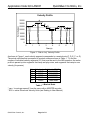
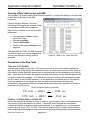
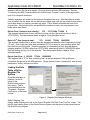
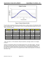
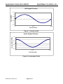
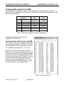
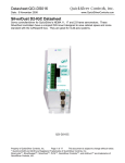
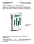
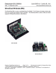
Application Note:QCI-AN031
Date: 12 November 2004
QuickSilver Controls, Inc.
www.QuickSilverControls.com
Interpolated Motion Control - Standalone
Associated Files:
• Profile Playback – Ode to Joy.qcp
• Profile Playback – Ode to Joy.txt
• Profile Playback - Position(t).qcp
• Profile Playback - Position(t).txt
• Make IMS Segment.xls.
Introduction
For many industrial camming applications, it is necessary to define a motion profile with
velocity segments. The Interpolated Motion feature allows users to execute interpolated
movements by utilizing four Data Registers that cycle through Time, Position, Acceleration,
and Velocity Data. See Interpolated Motion Control in SilverLode User Manual for a general
description.
These registers define constant acceleration velocity segments that ramp (up or down) to a
desired velocity or move at a constant velocity (acceleration = 0) over a period of time. By
streaming data through these registers, the IMS command can interpolate the points in each
velocity segment as well as between the velocity segments to create a continuous, complex
motion profile.
The cycling of data can be accomplished either by a host that streams the data to the device
via serial communication or by the device operating in a standalone configuration. This
document will focus on standalone-interpolated movement where all data resides in the QCI
device's non-volatile memory and is spooled to the IMS command via a Register File Array
command. Two specific application examples are provided in this application note; one that
details using velocity over time data (ode to joy) and another that details position over time
data (sinusoidal motion).
Velocity over Time Data – Ode to Joy Example
The easiest and most straightforward way to understand IMS is within an application where the
data is defined by velocity as a function of time—as in the Ode to Joy example. In this
application, moves of different velocities create musical notes and the duration of the note is
defined by how long the servo maintains that velocity. The velocity profile is defined so that it
ramps up or down to specific velocities that coincide with the musical notes of “Ode to Joy”.
Property of QuickSilver Controls, Inc.
Page 1 of 11
This document is subject to change without notice.
QuickControl® is a registered trademark of QuickSilver Controls, Inc.
Other trade names cited are property of their explicit owner.
QuickSilver Controls, Inc.
Application Note:QCI-AN031
Velocity Profile
35000
G
F
Velocity (cps)
30000
E
25000
D
C
20000
15000
10000
5000
0
0
1
2
3
4
5
6
7
Time (s)
Figure 1: “Ode to Joy” Velocity Profile
As shown in Figure 1, each velocity segment corresponds to a musical note (C, D, E, F, or G).
The actual velocities that correspond to musical notes are shown in Table 1. To find the
number of individual velocity segments (21) that must be sent to the IMS operation, the entire
profile is parsed up into segments that ramp and play notes, and segments that ramp to zero
velocity (for pauses).
Note Velocity (cps*) Velocity (SVU*)
G
31360
252544077
F
27960
225163660
E
26360
212278758
D
23480
189085935
C
20920
168470092
Table 1—Musical Scale
* cps = “counts per second” from the servo with a 4000CPR encoder
* SVU = native SilverLode Velocity Units (see Scaling in User Manual)
QuickSilver Controls, Inc.
Page 2 of 11
QuickSilver Controls, Inc.
Application Note:QCI-AN031
Creating a Data Table for Use with IMS
The Register File System within QuickControl revision 4.0 + permits the linking of text files that
contain data to be used by the IMS
command.
Figure 2 shows a Register File Array
consisting of 22 rows and 4 columns. Each
row specifies an IMS velocity segment.
Each column contains one of the four IMS
parameters.
•
•
•
•
First parameter is time (in servo
cycle clock ticks)
Second is position
Third is acceleration
Fourth is the ending velocity of that
segment.
This data table will “feed” the IMS command
one line at a time (one velocity segment at
a time) until the entire velocity profile is
executed.
Figure 2: “Ode to Joy” Data Text File
Parameters of the Data Table
Time: 0 to 2,147,483,6471
Indicating the number of time ticks (120 µsec time slices) to count down before loading the
next set of data. Note that the time parameter does not influence the motion profile; it acts as
a time delay, giving the profile enough time to develop based on the acceleration and velocity
data. If this value is too small, the segment will end prematurely, too big, and the segment will
run on for longer then intended. A “0” indicates the last set of data to be transferred and tells
the QCI device to exit the IMS operation. In this application, the values chosen for segment
times are indicative of note length, but their corresponding parameters (velocity and
acceleration) are calculated from the constant acceleration kinematics equations of motion to
make the song “Ode to Joy”.
Time Conversion (ticks to seconds)
270 ticks × . 00012
3470 ticks × . 00012
sec
tick
sec
tick
= . 0324 sec
= . 4164 sec
Position: -2,147,483,648 to 2,147,483,647
Unless the segment is intended to come to a halt at a given location, the position parameter is
only used to project the direction of motion. It should be noted that position calculations
incorporate register wrap-around as they are summed. For a general move, use the present
position, plus or minus 1,073,741,824. This value is large enough to project moves properly,
while remaining small enough to never wrap around the register range and project movement
QuickSilver Controls, Inc.
Page 3 of 11
QuickSilver Controls, Inc.
Application Note:QCI-AN031
in the opposite direction. If the segment should stop (decelerate to zero velocity), give the
desired ending position of the move. In this case, the position parameter is used to direct the
motion profile to a specific location.
Note that in Figure 2, all but two position parameters are large positive values to project each
velocity segment out to infinity. The 21st segment commands a decelerating stop from the last
“D” velocity, so the final stopping position is given. The 22nd segment has a “0” for time
commanding an exit from IMS and indicating it is the last segment. Since they have no effect,
the previous position, velocity, and acceleration parameters are repeated.
Acceleration: 1 to 1073741823 (Scaled from a 0 – 2000RPM/120µsec value)
This parameter has the highest priority and defines the acceleration or deceleration used in
reaching the ending velocity of the segment. A “0” indicates a constant velocity segment.
Acceleration is calculated from time using constant acceleration kinematics equations of
motion. See SilverLode Acceleration Units (SAU) in User Manual for scaling details.
Acceleration Conversion With 4000CPR Encoder (cps/s to a SAU)
3865.47056
sec 2
rev
× 800000
counts
sec 2
×
1rev
= 773094
4000 counts
Velocity: 0 to 2,147,483,647 (Scaled from a 0 – 4000RPM value)
Unless the segment is the last of the profile, this should be the desired ending velocity of the
segment. When specifying the last segment of a profile, set velocity equal to the starting
velocity of the segment. Do not set it to the ending velocity of the segment (usually 0); this will
cause the servo to undershoot the desired ending position. See SilverLode Velocity Units
(SVU) in User Manual for scaling details. The musical scale (shown in Table 1) define the
velocities used, which are given by:
Velocity Conversion With 4000CPR Encoder (cps to a SVU)
32212254.7
sec
rev
× 31360
counts
sec
×
1rev
= 252544077
4000 counts
Explanation of the Data Table
The first row of the Register File Array shows a velocity segment that ramps up to the “E” note
velocity and projects that movement for 3470 ticks (0.4164 sec) before looking to load a new
segment or decelerate to a stop using register 19. Note that these parameters define the initial
ramping and constant velocity segments, while the position specified for this segment is never
reached. The position parameter is intended to allow the acceleration and velocity parameters
to define the shape of the profile while position is projected off to some unattainable position.
Data in Row 1 (ramp and play “E”): 3470 2147483647 773094 212278758
The 3470 ticks of time data are copied to register 18 just before this segment’s execution. This
count is decremented every servo cycle (120 µsec) until it reaches “0”. If register 17 has been
written to, it should contain the register reference number of the first register out of four user
registers from which to load data. If register 17 still has a “1” in the upper word, the IMS
QuickSilver Controls, Inc.
Page 4 of 11
Application Note:QCI-AN031
QuickSilver Controls, Inc.
operation will use the value in register 19 to stop motion and exit IMS operation. See the
“Configuring the IMS Command within the QuickControl Program” section of this application
note for a complete discussion.
Velocity segments are defined in this manner throughout the song. Note that when a double
note is played, the two notes are not defined as a single long note, but two distinct notes with a
quick ramp down to 0 velocity and back up again. This is done to maintain the beat of the
original tune. If the double notes are profiled as a continuous note, the tune reduces to ten
beats rather then fifteen.
Data in Row 2 (ramp to zero velocity):
270 1073741824 773094 0
This segment ramps down to zero velocity but does not stop (the position value is left at
1073741824). Time decrements down in register 18 as described above.
Data in 21st Row (ramp to stop):
272 161000 773094 189085935
This segment ramps down to a stop using the standard acceleration after completing the final
“D” note. Give a few extra ticks than calculated (270+2) to allow for any rounding errors that
have built up over the profile. Since the segment is commanding a stop, give the desired
stopping position (161000) rather than 1073741824, and starting velocity (189085935) rather
than the ending velocity (0) of the segment. Time decrements down in register 18 as
described above.
Data in final Row: 0 161000 773094 189085935
This segment has a “0” for time, indicating that it is the last segment of the profile and
commands the device to exit IMS operation. Simply repeat position, acceleration, and velocity
parameters, as they will have no effect.
Linking the Data
Table with the
Register File
System
Once the data table is
created, it must be
linked to the
QuickControl program
that uses it. This is
accomplished with the
“Programs > Register
Files” option in the main
toolbar.
Figure 3: Register file Dialogue Windows
Select “Register File
Arrays” under Display and click on the “Import Register File Data From Text File” button. The
text file that is being linked to the QuickControl program must be saved to the same folder as
the QuickControl program.
QuickSilver Controls, Inc.
Page 5 of 11
Application Note:QCI-AN031
QuickSilver Controls, Inc.
Configuring the QuickControl Program to use the Register File System
Once the text file is linked, the QuickControl Program
needs to access the register file properties so that it can
iterate through the entire array. Three Write Register
File (WRF) commands are needed to do this. The first
WRF command writes the non-volatile memory Start
Address, where the first row of data resides, to a user
register. The register file system assigns the start
address automatically upon linking to ensure that the
entire table will fit in non-volatile memory. The second
WRF command writes an Address Increment to another
register. The register file system assigns an address
increment based on the number of columns reported
(col=4, see Figure 2) in the first line of the Register File
Figure 4: WRF Dialogue
Array. The third WRF command writes the Number of
Rows in the array to a third register. Specified in the first line of the Register File Array
(row=22, see fig. 2). See Register File System in SilverLode™ User Manual for details.
Configuring the IMS Command within the QuickControl Program
Once three user registers contain the Start Address, Address Increment, and Number of Rows
of the table, the IMS command has to start iterating through the data. The IMS command uses
seven registers in its operation. Register [17] contains a data indicator (see Checking for Stale
Data) in the upper word and the register reference number of the first user register that is
loaded with segment data in the lower word. Register [18] is used internally to hold the
segment time countdown. Register [19] holds a data loss deceleration value. This value will
only be used if there is an under-run of data to the IMS operation; the time value counted down
in Register [18] reaches zero before a new velocity segment is loaded into the user registers.
The four user registers are defined by the value in Register
[17]. The first holds the time data, the second position data,
the third acceleration data, and the fourth register holds
velocity data. In “Profile Playback – Ode to Joy.qcp” these
are Registers [30] – [34].
After the operational registers are loaded with data and the
four segment data registers are identified, they should be
loaded with the first row of segment data from the Register
File Array. This is accomplished via indirect addressing and
the Register Load Multiple (RLM) command. With the
“Indirect Addressing Mode” checkbox checked, the RLM
command uses the value in the Accumulator [10] as the
starting non-volatile memory address of the data to be
loaded into the segment data registers. Therefore, before
the RLM is issued, the Start Address from the first WRF
Figure 5: RLM Dialog window
must be copied into the Accumulator [10]. Then the RLM is
issued, loading registers 30-34 with time, position, acceleration, and velocity data.
After the first segment is queued into the data registers, the IMS command starts execution.
The IMS command requires two tasks running in a loop to ensure that it can iterate through the
QuickSilver Controls, Inc.
Page 6 of 11
Application Note:QCI-AN031
QuickSilver Controls, Inc.
entire Register File Array. This loop checks to see if the segment data just loaded has been
used, then queues the next row of data into the same four registers. If the next segment is not
loaded into data registers before the previous segment ends, the IMS command uses the
acceleration value in Register [19] to come to a stop and exits IMS operation.
Checking for Stale Data
Register [17] is an operational register for the IMS command, and contains the register
reference number of the first register that is loaded with segment data. Once the IMS
operation copies the segment data, it writes a “1” to the upper word of Register [17] indicating
the data is stale.
When fresh data is loaded, Register [17] must have the register reference number rewritten in
order to clear the upper word “0000XXXX” and once the data is stale, the IMS operation
automatically writes a “1” to the upper word “0001XXXX” (in “Ode to Joy” XXXX is 001E, 30 in
hex). A single Jump on Register Equals (JRE) command back to itself when Register [17]
indicates fresh data is present (Reg17=0000001E) can serve as a single line checking routine.
As soon as the “1” is written to the upper word, the jump condition is no longer valid, and the
loop moves on to the next task.
Queuing the Next Row of Data
Once the previous segment is stale, the loop needs to load (with the RLM command) the next
row of data into the segment data registers. To achieve this, the current Start Address must
be added to the Increment Address; the resulting sum is the Start Address of the next row of
data in the Register File Array. This is the new value that must be copied into Accumulator
[10] before the RLM command executes. Note: See the “CHECK” loop in Profile Playback –
Ode to Joy.qcp for an example of this routine.
This loop should iterate through the entire Register File Array with no problems. Similar
routines can be implemented for use with the IMS command, but care should be taken to
ensure that they execute in a timely manner. If the loop is trying to do too many tasks in
between checking for stale data and loading the new data, a data under-run could occur
causing the interpolated move to decelerate to a stop using Register [19] and exit prematurely.
If it is necessary to repeat the profile or exit the program after the profile is finished, use the
Calculation (CLC) command to decrement the Number of Rows register each time the loop
executes, and use the JRE command when that register contains a “0” to jump to an exit line
or repeat the process.
Position Over Time Data – Sinusoidal Motion Example
In this example, position vs. time data for a cosine function will be used to create a table to
follow the cosine curve. Figure 6 shows the original position function defined by an inverted
cosine function shifted for positive displacement over t = 0 to t = 2π.
QuickSilver Controls, Inc.
Page 7 of 11
QuickSilver Controls, Inc.
Application Note:QCI-AN031
Original Function
Position (Revs)
1.2
1
0.8
0.6
0.4
0.2
0
0
3.14
6.28
Time (Seconds)
Figure 6: Desired Position Profile
From this data, successive derivatives should be taken to obtain velocity and acceleration data
for the original profile. This can be done in Excel or another spreadsheet program as shown in
Table 2 on the next page.
Pos (revs)
Time (sec)
dx (revs)
dt (sec)
Vel (rps)
Acc (rps/s)
0.5 - 0.5*cos(time)
(k* π)/n
k=0,1,2…n=25*
posn-posn-1
timen-timen-1
dx/dt
veln-veln-1/dt
0
0.007885285
0.031416786
0.070223397
0.123693115
0.190982694
0
0.1256636
0.2513272
0.3769908
0.5026544
0.628318
0.00789
0.02353
0.03881
0.05347
0.06729
0.1257
0.1257
0.1257
0.1257
0.1257
0
0.06
0.19
0.31
0.43
0.54
0
0.99081
0.967309
0.928554
0.875154
0.807953
Table 2: Example Velocity and Acceleration Spreadsheet
* Note: The value n = 25 is chosen for 50 point resolution, use larger values of n for higher
resolution.
Velocity and acceleration data can be plotted against time to verify data integrity. Since the
derivative of position yields velocity, and the derivative of velocity yields acceleration, these
plots should be visually examined to verify correct velocity and acceleration calculations. In
this case, the choice of cosine for the original function makes visual inspection of successive
derivatives easy.
QuickSilver Controls, Inc.
Page 8 of 11
QuickSilver Controls, Inc.
Application Note:QCI-AN031
d/dt Original Function
Velocity (RPS)
1.5
1
0.5
0
-0.5
-1
-1.5
0
3.14
6.28
Time (seconds)
Figure 7: Velocity Profile
Acceleration (RPS/S)
d2x/dt2 Original Function
1.5
1
0.5
0
-0.5
-1
-1.5
0
3.14
Time (Seconds)
Figure 8: Acceleration Profile
QuickSilver Controls, Inc.
Page 9 of 11
6.28
QuickSilver Controls, Inc.
Application Note:QCI-AN031
Creating Data Segments for IMS
Interpolated Move segments can also be computed within a spreadsheet from the actual
position, velocity, acceleration, and time data. Following the rules for each parameter, an IMS
table is generated below.
Interpolated Move
Segments
Time (ticks)
Position (counts)
dt/0.00012 poscurrent±1073741824
Acceleration
(SAU)
Velocity
(SVU)
0-2 -1:
0-2000RPM/120usec
30
0-2 :
0-4000RPM
acc*3865.47056
vel*32212254.705
31
1047
1073741824
1914
1010645
1047
1073741840
1869
3015999
1047
1073741888
1794
4973788
1047
1073741966
1691
6853138
1047
1073742073
1561
8624410
Table 3: IMS Data Segments Defined in Spreadsheet
See Make IMS Segments below for an
explanation of the XLS file.
Creating a Data Table for Use with IMS
Just as in the “Ode to Joy” example, a data table
can be made and linked to a QCP file. The data
for this application can be copied directly out of
the spreadsheet and pasted in to the .txt file.
Notice that the 50th row has a few extra ticks
added for any rounding errors that may have built
up and the position is set as the desired stopping
position of the profile as described earlier. Also,
note that an extra row (the 51st) with a “0” for time
has been added with repeated parameters for
position, velocity, and acceleration. The “0” for
time initiates an exit from IMS operation, a very
important step if this is the desired action.
Figure 9: Position Data Text File
QuickSilver Controls, Inc.
Page 10 of 11
Application Note:QCI-AN031
QuickSilver Controls, Inc.
Make IMS Segments
The Make IMS Segments.xls spreadsheet example uses time data in π/25 increments (column
B). For a more precise approximation, use smaller fractions of π for the time interval; this will
also require more data points. Position is a cosine function of time (column A) and that is why
time increments were chosen as a fraction of π. Increase the fraction to π/50 to yield a much
better approximation.
The encoder constant (D2) only applies to scaled position data (position in counts columns
G&H) and the final position column for the IMS segment (column N).
Columns F-K use the finite difference between time and position to generate velocity (dx/dt)
and acceleration (d2x/dt2) data. Columns J & K are plotted against time for the velocity and
acceleration plots respectively. A COS function for position was chosen because successive
derivates (velocity and acceleration) are easily identified: vel= -SIN and acc= -COS (see the
first three plots).
Note that the start and end points of actual velocity (dx/dt) and acceleration (d2x/dt2) are hilighted in red. This is to indicate that the endpoints of dx/dt can cause a spike in d2x/dt2 and in
some instances needs to be inputted manually rather then calculated by the spreadsheet. It
was noticed that adjustments to these endpoints were needed to realize a more precise move
(final position ±1 count around 0). If the actual acceleration plot was let to begin and end on –
1 (as it should), the final position was short 30 counts or so.
Once the position function and it's successive derivatives are confirmed graphically, compute
the actual IMS data segments (cols M-P). Click on a cell in columns M-P to see the constants
used to scale actual position, velocity, and acceleration data into Native SilverLode Units
based on the register range for each parameter used by IMS.
A slight gain (10% or lower) is added to the acceleration and velocity data. These gains need
to be equal or else the ending position of the profile is negatively affected. The gains are used
to increase the peak position of the COS curve. With the original calculated values, the actual
position curve falls short of the peak value.
Important Notes
Interpolated time is in SilverLode servo clock ticks: dt/120usec and is rounded down to the
nearest integer. It was noted that this, along with rounding interpolated velocity and
acceleration up, yields precise moves (most of the time stopping exactly on 0 and oscillating
±1 count).
Interpolated position is NOT the position each segment is commanded to; it is only used to
project the move in a direction. IMS position is defined to be: current position +1073741824 if
actual velocity is in the positive direction or -1073741824 if actual velocity is in the negative
direction. See the Interpolated position graph and the "IF" statement in the cell formatting.
Interpolated velocity and acceleration are scaled absolute values; they do not need a sign
because the position parameter will be projecting the direction of the segment. See the
Interpolated plots and cell formatting for constants used.
QuickSilver Controls, Inc.
Page 11 of 11