1
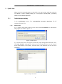
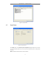
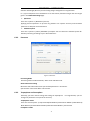
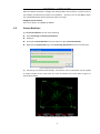
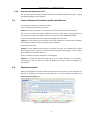
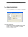
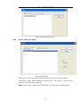
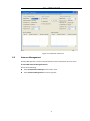
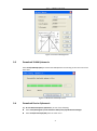
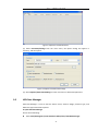
CGO | CHC GEOMATICS OFFICE USER MANUAL I Introduction About this Manual Welcome to the CHC Geomatics Office Manual. This manual is designed to provide the information that you need to effectively use the full power and capabilities of CHC Geomatics Office, hereafter referred to as CGO. It also describes how to install and use CGO software. Revision December 2013 – Version 1.0.1 Technical Support If you have a problem and cannot find the information you need in the product documentation, contact the CGO support center. Your Comments Your feedback about the supporting documentation helps us to improve it with each revision. E-mail your comments to [email protected]. World Wide Web site For an interactive look at CHC Navigation, visit our site on the World Wide Web (www.chcnav.com). Disclaimer Please read this user guide before using the software so that it can be used in a proper way. CHC Navigation holds no responsibility for the wrong operation. In addition, CHC reserves the rights to make changes of the user guide regularly. Copyright Copyright 2009-2013 CHC Shanghai HuaCe Navigation Technology Ltd. All rights reserved. II CONTENT INTRODUCTION ............................................................................................................................................................ II CONTENT ...................................................................................................................................................................... 1 1. QUICK START ................................................................................................................................ 4 1.1 STATIC DATA PROCESSING ........................................................................................................................... 4 1.1.1 New Project ......................................................................................................................................... 4 1.1.2 Import Data ......................................................................................................................................... 5 1.1.3 Process Baselines ................................................................................................................................ 6 1.1.4 Known Points Settings ......................................................................................................................... 9 1.1.5 Adjustment .......................................................................................................................................... 9 1.1.6 Result Output .................................................................................................................................... 10 1.2 POST-PROCESS KINEMATIC (PPK) DATA ...................................................................................................... 11 1.2.1 New Project ....................................................................................................................................... 11 1.2.2 Import Data ....................................................................................................................................... 11 1.2.3 Process Baselines .............................................................................................................................. 11 1.2.4 Result Output .................................................................................................................................... 12 2 USER INTERFACE ..........................................................................................................................13 2.1 INTRODUCTION ...................................................................................................................................... 13 2.2 STARTUP OF CGO .................................................................................................................................. 13 2.3 MENU................................................................................................................................................. 14 2.4 TOOLBARS ............................................................................................................................................ 15 2.5 PROJECT BAR ........................................................................................................................................ 15 2.6 WORKING AREA .................................................................................................................................... 16 2.6.1 Project Plot ...................................................................................................................................... 16 2.6.2 Files Page ......................................................................................................................................... 17 2.6.3 Baselines Page ................................................................................................................................. 18 2.6.4 Stations Page ................................................................................................................................... 20 2.6.5 Loops Page ....................................................................................................................................... 20 2.7 OUTPUT WINDOW ................................................................................................................................ 20 2.8 STATUS BAR.......................................................................................................................................... 20 3 PROJECT MANAGEMENT .............................................................................................................20 3.1 CREATE A NEW PROJECT .......................................................................................................................... 20 3.2 OPEN A PROJECT.................................................................................................................................... 21 3.3 SAVE A PROJECT..................................................................................................................................... 22 1 3.4 CLOSE A PROJECT ................................................................................................................................... 22 4 PROJECT COORDINATE SYSTEM AND ATTRIBUTE .........................................................................22 4.1 PROJECT DETAIL ..................................................................................................................................... 22 4.2 PROJECT DATUM .................................................................................................................................... 23 4.3 TIME SYSTEM ........................................................................................................................................ 24 4.4 UNIT AND FORMAT................................................................................................................................. 25 4.5 ADVANCED ........................................................................................................................................... 25 5 DATA IMPORT ..............................................................................................................................26 5.1 OBSERVATION DATA FORMAT.................................................................................................................... 26 5.2 DOWNLOADING DATA FROM A RECEIVER .................................................................................................... 27 5.3 IMPORT DATA ........................................................................................................................................ 27 5.4 OBSERVATION FILE ATTRIBUTE DIALOG ....................................................................................................... 28 5.5 SATELLITE TRACK DIALOG......................................................................................................................... 28 5.6 IMPORT PRECISE EPHEMERIS .................................................................................................................... 30 6 PROCESS BASELINES ....................................................................................................................30 6.1 BASELINES PROCESSING OVERVIEW ........................................................................................................... 30 6.2 BASELINE PROCESS PARAMETERS DIALOG.................................................................................................... 31 6.2.1 General Settings ................................................................................................................................ 31 6.2.2 Processor ........................................................................................................................................... 33 6.2.3 Troposphere and Ionosphere ............................................................................................................ 33 6.2.4 Advanced Settings ............................................................................................................................. 34 6.3 PROCESS BASELINES................................................................................................................................ 35 6.4 CHECK BASELINE PROCESS RESULTS ........................................................................................................... 36 6.4.1 Baseline quality control ..................................................................................................................... 36 6.4.2 Loop and Repeated baseline check ................................................................................................... 36 6.4.3 Free Network Adjustment check ....................................................................................................... 38 6.5 FACTORS INFLUENCE ON BASELINE RESULTS AND SOLUTIONS........................................................................... 38 6.6 REPROCESS BASELINE .............................................................................................................................. 38 7 NETWORK ADJUSTMENT .............................................................................................................39 7.1 NETWORK ADJUSTMENT OVERVIEW .......................................................................................................... 39 7.2 PREPARATION BEFORE NETWORK ADJUSTMENT ............................................................................................. 40 7.2.1 Coordinate system settings and Network Check ............................................................................... 40 7.2.2 Network Adjustment settings ........................................................................................................... 40 7.2.3 Set Control Point ............................................................................................................................... 42 7.3 ADJUSTMENT ........................................................................................................................................ 43 7.4 RESULTS ............................................................................................................................................... 45 2 8 REPORTS......................................................................................................................................46 8.1 BASELINE PROCESSING REPORT ................................................................................................................. 46 8.1.1 Static Baseline Processing report ...................................................................................................... 46 8.1.2 Kinematic Baseline process report .................................................................................................... 46 8.2 LOOP REPORT........................................................................................................................................ 47 8.3 ADJUSTMENT REPORT ............................................................................................................................. 48 8.4 ADDITIONAL REPORT ............................................................................................................................... 49 8.5 DATA EXPORT ........................................................................................................................................ 49 8.5.1 Baseline Computation Result Export ................................................................................................. 49 8.5.2 DXF file and log file Export ................................................................................................................ 50 8.5.3 Project summary Report ................................................................................................................... 51 9 TOOLS ..........................................................................................................................................51 9.1 COORDINATE TRANSFORMATION ............................................................................................................... 51 9.2 ANTENNA MANAGEMENT ........................................................................................................................ 52 9.3 DOWNLOAD YUMA EPHEMERIS ............................................................................................................... 53 9.4 DOWNLOAD PRECISE EPHEMERIS .............................................................................................................. 53 9.5 HCN DATA MANAGER ............................................................................................................................ 54 9.6 RINEX CONVERTER TOOL ........................................................................................................................ 55 10 INSTALLATION AND REGISTRATION..............................................................................................57 10.1 SYSTEM REQUIREMENTS .......................................................................................................................... 57 10.2 INSTALLING CGO ................................................................................................................................... 57 10.3 SOFTWARE REGISTRATION........................................................................................................................ 59 APPENDIX ....................................................................................................................................60 1. TERMINOLOGY ..................................................................................................................................................................... 60 2. SP3 PRECISE EPHEMERIS........................................................................................................................................................ 62 3. YUMA ALMANAC FORMAT.................................................................................................................................................... 66 4. SHORTCUT KEY .................................................................................................................................................................... 67 3 Process Baselines——CGOffice User Guide 1. Quick Start Below are the recommended steps in using CGO. This step-by-step guide will quickly get you started on CGO, including setting up a new project, importing data, processing baselines, and network adjustment. 1.1 Static data processing In the Start/Programs menu select HuaceNAV/CHC Geomatics Office/CGO. It will automatically start CGO. 1.1.1 New Project (1) To create a new project, select the main menu command File/New. The New Project dialog appears, as shown in Figure 1-1. Figure 1-1 New Project (2) Enter the name of the new project, set the new project storage path and click OK. Then, the Project Attribute dialog appears. Note that the new dialog presents five tabs: Project Detail, Project Datum, Time System, Unit and Format, and Advanced. You can edit these parameters. Figure 1-2 Project Attribute 4 Process Baselines——CGOffice User Guide (3) Click Project Datum to switch to the Project Datum tab (see Figure 1-3). Then Click change button, and coordinate system management dialog will appear, as shown in Figure 1-4. Figure 1-3 Project Datum (4) Define your coordinate system, and click OK. Figure 1-4 Coordinate System Management (5) Click OK. Now you have finished setting up a new project. 1.1.2 Import Data After creation of the project, you can import raw data to process. 5 Process Baselines——CGOffice User Guide (1) Click File/Import/Source File (or Hotkey F1), the Import Files dialog will appear. Choose the type of data you want to import. Select the files to import and click ok. Check Source Data dialog will appear. Figure 1-5 Check the Source Files (2) Check and if necessary, edit the following parameters: point name, Antenna Height, Antenna Type, Survey Type. Then click OK. (3) After that, CGO automatically displays the network plot, observation file list, baseline list, station list and so on. You can also edit point name, Antenna Height, Antenna Type, Survey Type in Files page. Figure 1-6 Plot 1.1.3 Process Baselines (1) Set parameters. Select Processing/Config Baseline Processing All Baselines from the main menu( or Hotkey F2). Then Baseline Process Parameters dialog appears. If necessary, you can modify the default parameters. 6 Process Baselines——CGOffice User Guide Figure 1-7 Baseline Process (2) Process Baselines Select Processing/ Processing All Baselines from the main menu (Hotkey F2). Figure 1-8 Processing Baselines Wait until Baseline Processing dialog disappears. 7 Process Baselines——CGOffice User Guide Figure 1-9 The Network Diagram after Baseline Processing NOTE: Green: quality test was successful. Yellow: quality test failed. (3) If you are not satisfied with the results, check, for example, reference station coordinates, check parameters, check observations (select the baseline Residual Graph from right click menu as shown in Figure 1-10, delete bad observations as shown in Figure 1-11 ). Then repeat processing. Figure 1-10 Baseline Residual Graph Command 8 Process Baselines——CGOffice User Guide Figure 1-11 Observation and Residual Map (4) View results. Select Report/Baseline Processing Report from the main menu. 1.1.4 Known Points Settings Select Adjustment/Setting Known Points (Hotkey F6), the Input known points dialog appears, as shown in Figure 1-12. You can edit the coordinates of control points and select the constraint type. Figure 1-12 Setting Known Points 1.1.5 Adjustment (1) Select Adjustment/Adjustment (Hotkey F5), the Adjustment dialog appears, as shown in Figure1-13. 9 Process Baselines——CGOffice User Guide Figure1-13 Adjustment (2) If necessary, Click Settings button to set the adjustment parameters. (3) Select the type of Constraint Adjustment and Height Fitting, then click adjust button. The software will automatically complete the adjustment operation. 1.1.6 Result Output (1) Click Report button as shown in Figure1-13 or select Report/Adjustment Report, the adjustment report will be generated automatically. Figure1-14 Adjustment Report (2) To export the results in word format, you can select File/Export from the main menu, and the Export dialog will appear. Switch to the Project Summary Report to export the document. 10 Process Baselines——CGOffice User Guide 1.2 1.2.1 Post-Process Kinematic (PPK) data New Project Refer to 1.1.1 New Project. 1.2.2 Import Data Refer to 1.1.2 Import Data. Figure 1-15 PPK Project Plot 1.2.3 Process Baselines (1) Check Switch to Files tab to check the station name, Antenna Height, Antenna Type, and Survey Type. If necessary, you can edit them. (2) Setting Known Point If you want to set control base points, switch to Station tab, right-click a base point and select from its context menu the option Setting Known Points. Then, the PPK Setting Known Point dialog appears, as shown in Figure 1-16. 11 Process Baselines——CGOffice User Guide Figure 1-16 Setting Known points Select constraint type and enter the coordinates in setting known point dialog, then click ok. (3) Process baselines Select Processing/ Processing All Baselines from the main menu (Hotkey F2). Figure 1-17 PPK plot 1.2.4 Result Output Select Report/ Baseline Report, the baseline report will be generated automatically. 12 Process Baselines——CGOffice User Guide Figure 1-18 PPK Report 2 User Interface 2.1 Introduction This chapter gives you an overview of all basic objects involved in CGO interface. 2.2 Startup Of CGO To start CGO Do one of the following: Select Start/Programs menu select HuaceNAV/CHC Geomatics Office/CGO. Double-click the desk icon Once start CGO, the software main interface appears as shown in Figure 2-1. 13 Process Baselines——CGOffice User Guide Figure 2-1 CGO Main Interface After creating or opening a project, the interface will appear, as shown in Figure 2-2. It consists of menu bar, toolbars, Project bar, working area, output window and status bar. Figure 2-2 Software Interface 2.3 Menu The main menu consists of File, Edit, View, Processing, Adjustment, Report, Tool, Window, and Help options. Figure 2-3 Menu Bar 14 Process Baselines——CGOffice User Guide Besides main menu, each window has a context menu. The commonly used menu items have their own hotkeys. You can complete most processes by the submenu items, which covers the main processes of each step. 2.4 Toolbars CGO has powerful toolbars. Located just below the menu bar, they act as a graphical Control center, where you may access the module’s most commonly used functions with the click of a mouse button. A toolbar consists of one or more tools. Toolbars are separated by vertical lines. A tool is a shortcut to frequently-used menu commands. A toolbar button displays the same icons as the respective menu command. Figure 2-4 Toolbars (1) New Tool: Create a new project. (2) Open Tool: Open a project. (3) Save Tool: Save a project. (4) Import Tool: Import data. (5) Export Tool: Export results. (6) Process Chosen baseline Tool: Process baselines Selected. (7) Process all baselines Tool: Process all the enabled baselines. (8) Adjustment Tool: Do network adjustment. (9) Select tool: Selects one or more objects shown on the map. (10) Grabber tool: Shifts the map as instructed. The map shift directly results from the length and orientation of the segment you drag on the map. (11) Zoom In: Zoom in on the area where you click or drag. (12) Zoom Out: Zoom out from where you click or drag (13) Full Screen: Adjust the map scale so that all the visible objects present on the map can be seen. (14) Grid: Show the grid of the map. 2.5 Project Bar The Project bar consists of named groups that list shortcuts to commonly-used tasks in the CGO software. Each shortcut is available in a menu. To quickly access a task: 1. Click a shortcut on the Project bar. 2. Click a group to move to a different set of shortcuts. 15 Process Baselines——CGOffice User Guide Figure 2-5 Project Bar The navigator at the left-hand side shows a preliminary project structure consisting of project, Import, Process Baselines, Adjustment and Tool, etc. With a new project, these containers are all empty. 2.6 Working Area The working area at the right-hand side displays the background for a sketch of the project (the project plot) and some tables. At the time of creation, they are all empty. Now, you may import GNSS data like observation files or other raw data, ephemeris data, and then use CGO to view or process those data. 2.6.1 Project Plot Project plot will display points, baselines, error ellipse, plotting scale, latitude-longitude grids and so on, as shown in Figure 2-6. Points When import kinematic data, the filled rectangle represents rover points while the filled triangle represents base points. When import static data, the filled triangle represents control points and the filled circle represents common survey points. 16 Process Baselines——CGOffice User Guide Baselines They are defined by their start and end point. To activate a baseline, click on it. NOTE: Color of unprocessed Baseline— White Color of qualified processed Baseline—Green Color of unqualified processed Baseline—yellow Color of baseline selected ---pink Color of disabled baseline ---gray Error Ellipse A specialty of the project plot is the display of standard errors for each baseline after processing and for each point after network adjustment. Standard errors are displayed in form of position error ellipses with height error bars. A reference circle indicates as diameter of the circle the maximum derived standard deviation values of the currently activated objects in North or East. A reference bar right to it indicates the maximum standard deviation in height. Figure 2-6Netwrok map Context Menu Right-click on the project plot area, the context menu will appears. 2.6.2 Files Page Lists for each observation file storage path, the point name, start time, end time and time span of observation, the receiver serial number and the type of measurement (static or kinematic). It also gives full antenna information. Figure 2-7 Observation Files 17 Process Baselines——CGOffice User Guide Context Menu Right-click on the Files area, the context menu will appears. Figure 2-8 Observation Files Transform to RINEX file: Right click item Transform To RINEX to transform the original file again and then RINEX data would be saved in the RINEXs folder of the project folder. Delete: you can directly delete the chosen file. 2.6.3 Baselines Page Baseline table Open the table of baselines within the project. For each baseline, you will find information on ID, begin point, end point, solution, start time and time span of observation, ratio, rms, the baseline components dX, dY and dZ with standard deviations and the slope distance between the start and end point. Figure 2-9 Baselines list Context Menu Right-click on the baseline page, the context menu will appears. Figure 2-10 Baseline Right-Click popup Menu 18 Process Baselines——CGOffice User Guide Reverse Baseline: Reverse the begin point and end point. Enable/Disable Baseline: If checked, all baselines with sessions conforming to the selection will be enabled or disabled. Repeated Line Lists for repeated baseline group, the baseline components dX, dY and Dz, length difference, length difference tolerance and relative error. Figure 2-11 Repeated Line Observation and Residual Map Right-click on the baseline page, then select baseline residual graph from the context menu. The Observation and Residual Map Subpage will show up. You can use the observation edit tool (see below) to inspect baseline related observation data and to select the time spans to be used for processing. The screen displays the times of satellite tracking by two or more observation stations. You can edit the time span of collected data, disable selected satellite tracking information. You can also clear the check box to delete the bad satellite. Figure 2-12 Baseline observation data map At the bottom right corner, you can see the satellite Residual Graph, if you have process the baseline. Different color curves represent different satellite Residual error. The length of the time bar represents the total observation time from the left (start time) to the right (end time). Figure 2-13 Residual Graph 19 Process Baselines——CGOffice User Guide 2.6.4 Stations Page Lists for station name, local geodetic coordinates, north and east coordinate, height, parameters of constraints. You can set known points and delete stations by context menu. Figure 2-14 Stations List 2.6.5 Loops Page For each Loop, you will find information on ID, Loop Type, Quality, Loop Length, closure error components EX, EY, EZ and total length closure error E-Loop, number of baselines and relative closure error. It also gives baseline information that make up of the loop. Figure 2-15 Loops List 2.7 Output Window An output window documents many processes, warnings and errors. By default, it is positioned at the bottom of the working area. 2.8 Status Bar A status bar covers the bottom of the main window, displaying information: Whenever you move the cursor above a menu or toolbar item, a small text informs you about the action that will be performed when the item is chosen. 3 Project Management 3.1 Create a New Project To create a new project, do one of the following: Select the main menu command File/New. Click Click New Project from the Project bar. from the toolbar Project. 20 Process Baselines——CGOffice User Guide Hotkeys [Ctrl + Tab]. Figure 3-1 New Project Project Name: Default name is the assembly of local time, you can edit it Project Folder: Default path is the root folder of CGO.exe, you can change it The New Project dialog allows you to create a new project. When you click OK button, system will automatically create a folder with the name of the project, which consists of several subfolders, as shown in Figure 3-2. Figure 3-2 Project Subfolder Data Files: to save the result when saving the whole project; Eph Files: to save the Ephemeris files; Incoming: to save the future files related to the project, such as precise ephemeris files; Moving: to save the export baselines processed result; Obs Files: to save intermediate observation files; PEph Files: to save the downloaded precise ephemeris files; Reports: to save reports; RINEXs: this folder will save the source files’ RINEX files, if users execute the operation of transforming to RINEX. Additionally you may click Cancel button, if you don’t need it any more. 3.2 Open a Project To retrieve an already stored project from disk Do one of the following: 21 Process Baselines——CGOffice User Guide Select the main menu command File/ Open. Click from the toolbar Project. Click Open Project from the Project bar. 3.3 Save a Project To save ac project at any time: Do one of the following: Select the main menu command File/ Save. Click from the toolbar Project. The current project is stored with the same name with which it was opened or saved the last time. No dialog appears. 3.4 Close a Project To close the current project, select the main menu command File/ Close. When you close a project, a warning dialog will appear, asking you, whether you want to save changes to the project, or to leave the project without storing, or to cancel the closing process. 4 Project Coordinate System and Attribute After creation of a New Project, Project Attribute dialog will automatically show up. Use it to review and edit the status of your project. You will find all project-related information here. It contains four tabs. You can also select File/Project Attribute from the main menu or Click Project Attribute in project bar to open the dialog. 4.1 Project Detail Use it to view and edit the basic information of the project. 22 Process Baselines——CGOffice User Guide Figure 4-1 Project Detail 4.2 Project Datum Figure 4-2 Project Datum Click change button, the coordinate system management dialog will appear. You can select your local coordinates system here. You can create a new coordinate system or modify, delete an old one. NOTE: The default coordinate systems cannot be deleted. 23 Process Baselines——CGOffice User Guide Figure 4-3 Coordinate System Management 4.3 Time System It contains four time system: GPSW, GPST, UTC, Local time. If choosing local time, you can select the local zone from Choose Local Zone combo box. Figure 4-4 Time System 24 Process Baselines——CGOffice User Guide 4.4 Unit and Format Use it to view and edit the settings for the display of data units and format. Figure 4-5 Unit and Format 4.5 Advanced Use it to view and edit the advanced parameters of the project. Figure 4-6 Advanced Min. duration of static observation: The minimum simultaneous session in forming baselines for static processing. Min. duration of PPK observation: The minimum simultaneous session in forming 25 Process Baselines——CGOffice User Guide baselines for kinematic processing. Max. length of Baseline: If the distance between two points is greater than this value, it can’t form a baseline. Max. allowed distance between points: Stations will be considered as the same station if their distance is smaller than this parameter. Min. synchronous session: If the synchronous time is greater than this value, it can form a simultaneous observation loop; otherwise, it can form an independent observation loop. NOTE: The parameters of Advanced tab should be set before importing observation files. Or else they will not be effective. 5 Data Import 5.1 Observation Data Format CGO support the following data types: CHC type HCN file(*.HCN); V2.00 –V3.00 version RINEX file (*.??O, *.OBS); NOVATEL OEM4/V/6 mainboard file(*.NOV); TRIMBLE BD950/BD970 mainboard file(*.BD9); HEMISPHERE mainboard(*.RAW); Precise ephemeris file(*.SP3); Observation file mainly consists of original observation of each epoch, point information, ephemeris information and so on (see below). Figure 5-1 Observation Data 26 Process Baselines——CGOffice User Guide 5.2 Downloading Data From a Receiver First, transfer your data to computer. If using CHC GNSS receivers, you can download the data by HcLoader tool or U disk. When you use receivers with other brands, files should be transformed into standard RINEX format if it is not supported by CGO. 5.3 Import Data (1) To open the import dialog, , do one of the following: Select File/Import/Source File. Hotkey F1. Click option xx- Files from the Project bar group Import. The import dialog will show up. You can press Ctrl or Shift Key to select more files. NOTE: If a point that you want to import has the same name with a point already in the project, CGO checks for the position of the point. If the coordinates are apart more than the limit set in the Project Attribute dialog, a warning dialog will appear. When importing files, the software will automatically check the files, the output window will show related warnings. If a point that you want to import has the same receiver serial number, start and end time but different name from other points, CGO will automatically refuse to import, the warning bar in the message area will give the reasons for refusing. (2) After data being imported, a check dialog will appear. You can edit Station ID, point name, Antenna Height, Antenna Type and Survey Type. It allows you to deselect observation files from the import by clearing check box Figure 5-2 Check Source Data 27 Process Baselines——CGOffice User Guide 5.4 Observation File Attribute Dialog Right-click the Files page in the working area and then select Attribute option from the context menu, the Observation File Attribute dialog will appear. Figure 5-3 File Attribute Dialog Switch to Station tab, you can view or edit the station name Switch to Receiver tab, you can view the information of the receiver. Switch to Antenna tab, You can view, edit Antenna Height, Antenna type and survey type ,as shown in Figure 5-3 . 5.5 Satellite Track Dialog Right- click the Files page in the working area and then select Satellite Track option from the context menu, the dialog (see below) will appear. You can view single point positioning map, satellite track summary and SNR (Signal To Noise Ratio). 28 Process Baselines——CGOffice User Guide Figure5-4 Single Point Map Figure 5-5 Tracking Summary 29 Process Baselines——CGOffice User Guide Figure 5-6 Satellite Signal 5.6 Import Precise Ephemeris To import precise ephemeris (*.sp3), select File/Import/ Precise Ephemeris from the main menu. NOTE: If you select Precise Ephemeris in Baseline Process Parameter dialog, precise ephemeris will be used in baseline processing. 6 Process Baselines 6.1 Baselines Processing Overview CGO was designed for fully automated baseline calculation. To process your baselines, do the following: (1) Select baselines. (2) Set parameters. (3) Click the Process command. (4) Processing is performed automatically. (5) If necessary, re-compute. (6) View results. (7) If you are not satisfied with the results, check, for example, reference station coordinates, 30 Process Baselines——CGOffice User Guide check parameters, check observations. Then repeat processing. 6.2 Baseline Process Parameters Dialog To open Baseline Process Parameters dialog, do one of the following: Select Processing /Config Baseline Processing. Hotkey F4. Click option Baseline Process Parameters from the Project bar group Process Baselines. Right-click the project plot page, select Config Baseline Processing from the context menu. 6.2.1 General Settings Figure 6-1 General Settings Mask (Deg) The mask allows you to specify the minimum satellite elevation mask for post processing. Signals of low elevation satellite are complicatedly influenced by aerosphere and difficult to correct with models. Additionally, many factors such as multi-path and electromagnetic wave can put impact on them. Therefore, these signals are often poor and should be deleted in the post processing. 31 Process Baselines——CGOffice User Guide Figure 6-2 Elevation Mask Sampling interval (Sec) Enter a value for the processing interval given in seconds. The processing interval may be larger than the current observation time interval, but should be a multiple of it. This parameter is used to define the default sampling time interval in seconds between the epochs (observations) to be processed. This is useful when the data was recorded at a fast rate, e.g., every 0.5 seconds, and you want to process only every 10 seconds. This is also of importance considering that different processing intervals within a project would lead to different weighted observations in the Network Adjustment. GNSS differential processing is always optimistic with its analysis of standard errors and this effect is increased by a high processing frequency. Minimum Epoch Number CGO will consequently delete the data that contains less continuous epochs than the minimum epoch number requires. Minimum epoch number the software requires is two or more than two and the default number is five. The Observed carrier phase must be continuous to ensure the good quality of the baseline processing. Therefore, data with frequent cycle slips are poor-quality data and in most cases, should be deleted. Auto Processing There are 2 options: 1) Advanced 2) Common. If you select advanced option, the software will automatically eliminate the bad observation data and deal with the cycle slips; otherwise, you should delete bad data by hand. Frequency This defines the type of carrier phase to be used in the baseline processing. The following options are available: L1 only L1 processing only L2 only L2 processing only L1+L2 Combination of L1 and L2 data Ln "Narrow lane" phase combination with f=2803.02 MHz (L1+L2). Lw "Wide lane" phase combination with f=347.82 MHz (L1 - L2). This is useful for its low 32 Process Baselines——CGOffice User Guide effective wavelength (86.2 cm) and for finding integer ambiguities on long baselines. Lc > [x] km Ionospheric free combination of L1 and L2 data, if baseline longer than the length given in the Advanced Settings page. Ephemeris There are 2 options: 1) Broadcast 2) Precise; Applying Precise Ephemeris to process long baseline can improve accuracy and broadcast ephemeris is adequate to short baseline. Satellites System There are 3 options: 1) GPS 2) GLONASS 3) Compass. You can choose the satellites system for baseline processing according to your observation files. 6.2.2 Processor Figure 6-3 Processor Processing Mode Processing mode include Automatic, Static mode and PPK mode. Observation time setting Minimum static observation time span: default parameter is 10 minutes. Split sessions if start time differs: 120 minutes. 6.2.3 Troposphere and Ionosphere Generally, you don’t need to change the settings of Troposphere. For long baseline, you can change the parameters to improve the accuracy. Troposphere model There are several options: 1) Improved Hopfield Model 2) Sastamoinen Model 3) Niell Model 4) Black Model 5) Goad Goodman Model 6) New Brunswick Model 7) Uncorrected Ionosphere model 33 Process Baselines——CGOffice User Guide There are 2 options: 1) Auto 2) uncorrected Figure 6-4 Trop. and Iono. 6.2.4 Advanced Settings Figure 6-1 Trop. and Iono. Blunder tolerance coefficient Normally, the default setting is 3.5, and no need to edit. RMS and Ratio 34 Process Baselines——CGOffice User Guide When the RMS of the baseline is bigger than 0.04 and Ratio of the baseline is smaller than 1.8, the software will indentify the baseline as unqualified. Of course, you can edit RMS or Ratio. The unqualified baseline will be showed in Yellow in the plot. Ambiguity search method There are 2 options: 1) LAMBDA 2) OMEGA. 6.3 Process Baselines (1) To process baselines, do one of the following: Select Processing / Processing all baselines. Hotkey F2. Click option Process Baselines from the Project bar group Process Baselines. Right-click the project plot page, select Processing all Baselines from the context menu. Figure 6-6 Baseline process procedure (2) Processing is performed automatically. The baseline process information will be update on output window. At the same time, the color of baselines turns from white to green or yellow (disqualified). Figure 6-7 Baseline network after process 35 Process Baselines——CGOffice User Guide 6.4 6.4.1 Check Baseline Process Results Baseline quality control You can check the baseline quality by Ratio and RMS after baseline processing. RATIO The best ambiguity set found is compared to the second best. RATIO reflects the reliability of ambiguity and it depends on several factors like observation data quality and observation condition. RMS RMS (Root Mean Square): V:Residual error P:Weight of observation n-f:Redundancy RMS shows the quality of the observation value. The smaller the RMS value, the better the quality of observation value. RMS only indicates the precision of inner coincidence 6.4.2 Loop and Repeated baseline check The definition of loop closure Loop closure is a good way to check the baseline quality. Loop include: Simultaneous Observation Loop, Independent Observation Loop. Theoretically the loop closure should be zero, but in practice, it is not zero. Component error X Y Z X Y Z Relative closing error of loop X 2 Y 2 Z 2 S 36 Process Baselines——CGOffice User Guide S : Length of the loop Simultaneous Observation Loop Simultaneous loop is formed by synchronous baselines. Theoretically the synchronization loop closure should be zero. If synchronization loop closure exceeds the limit, it means at least one baseline of the loop have problem. If the closure is within the limit, it means most of the baselines are with good quality. Independent Observation Loop Independent Observation loop is consisted of asynchronous baselines. When independent observation loop closure is within the limit, it means the asynchronous baseline quality is good. If independent observation loop closure exceeds limit, it means there is at least one baseline of the loop have some problem. Repeated baseline The baseline between the two same observation stations during different time span is called duplicate baseline. How to Check Closure Error The content and tolerance range vary according to the setting of tolerance. The checking result will be displayed in the list of repeated baselines and closure loop. Figure 6-8 Loop For the unqualified closure loop and repeated baselines, the analysis and reprocess can be done as follows. a. Edit the closure loop and repeated baselines and reprocess these baselines until they are qualified. The editing method includes: delete some baseline observation data and sample interval according to baseline residual. b. Forbidden or delete some unqualified baselines. NOTE: The baselines of the loop should meet the following requirements: (1) Every baseline of the loop must be used. (2) Every baseline of the loop must be calculated. (3) The synchronized time of baseline group of loop should be no less than the minimum observational time. 37 Process Baselines——CGOffice User Guide 6.4.3 Free Network Adjustment check You can also check the baseline process results in Free Network Adjustment report. Please see following chapter for more details. 6.5 Factors Influence On baseline results and Solutions The main factors influence on baseline results: (1) The start point coordinate is inaccurate. Solution: The way to avoid this is to improve the accuracy of the start point coordinate. You can use the point with higher coordinate accuracy as start point. To get high accuracy coordinate, prolong static observation time or conjunct with other WGS84 coordinates. (2) Short satellite observation time causes that ambiguity can’t be fixed. Solution: You can delete the observation data of these Satellites or exclude these Satellites from baseline process to ensure the baseline process quality. (3) Too much cycle slips. Solution: If some satellites have big slips in the same time span, you exclude this time span from baseline process. If there are only some specific satellites have big slips, you can exclude these satellites from baseline process. (4) Error excessive caused by Ionosphere or troposphere. Solution: 1) Enlarge the elevation mask. But it is not always effective. 2) If the data is dual-frequency, you can select LC model. 3) Modify the correct model of Ionosphere or troposphere. 6.6 Reprocess baseline When you distinguish the factor impacting the baseline process result, you can reprocess the baseline by changing the baseline process parameters or edit the observation data in the observation and residual map. Figure 6-9 Baseline observation data and residual chat 38 Network Adjustment——CGOffice User Guide 7 Network Adjustment If satisfied with baselines processing results, you can continue with network adjustment and export results. 7.1 Network Adjustment Overview Generally Speaking, the network adjustment can be divided into following steps: (1) Before you start a network adjustment, set coordinate system, process baseline, import control points and run the Network Check in the Adjustment module. (2) Network adjustment and export results. (3) Quality check and analysis. Figure 7-1 Procedure of Network Adjustment You may want to temporarily exclude objects of your network from network adjustment. A lot of selection and toggling options, which are accessible from the main menu, from the project bar or from the project plot area, help you to configure your network. Before performing a least-squares adjustment, you can choose to hold the coordinates of one or several control point(s) fixed during adjustment. The project plot displays a little triangle to mark a fixed control point. NOTE: Note that fixed points will weigh very high within the adjustment. They force the adjustment module to adjust all others points in a way that they will fit the fixed points. Be 39 Network Adjustment——CGOffice User Guide sure that fixed points have very precise coordinates; otherwise they may induce geometrical distortions of your network. 7.2 7.2.1 Preparation before network adjustment Coordinate system settings and Network Check If necessary, select Project Attribute to open the attribute dialog and switch to project datum tab, then click change button to open Coordinate System Management dialog. You can check the coordinate system information here. Figure 7-2 Coordinate system management 7.2.2 Network Adjustment settings CGO allows you to modify a lot of parameters, which may influence the network adjustment. You may weigh the standard errors differently depending on the source of the data. You may perform a tau test and set tau test limits. You may define your own report format and make it known to the adjustment module. 40 Network Adjustment——CGOffice User Guide Figure7-3 Adjustment configuration-Quality Figure 7-4 Adjustment configuration-parameters 41 Network Adjustment——CGOffice User Guide Figure7-5 Adjustment configuration-Baseline Weighting 7.2.3 Set Control Point (1) To open Input Known points dialog, do one of the following: Select Adjustment /Setting Known Points. Hotkey F6. Click option Setting Known Points from the Project bar group Adjustment. Right-click the project plot page, select Adjustment from the context menu. (2) Set control points. Local If you choose Local, the constraint will list following options: 1) NE; 2) N,Zone+E;3) NEh; 4) N,Zone+E ;5)h; 6) BLH; 7) BL;8)None Figure 7-6 Local Point Input WGS-84 42 Network Adjustment——CGOffice User Guide If you choose WGS-84, the constraint will list following options: 1) XY 2) XYH 3) H 4) BLH 5) BL. Figure 7-7 WGS84 point Input NOTE: a. All the control point coordinates should be in the same coordinate system. b. The distribution of control points should be reasonable. 7.3 Adjustment (1) To open the Adjustment Dialog, do one of the following: Select Adjustment / Adjustment. Hotkey F5. Click option Adjustment from the Project bar group Adjustment. Right-click the project plot page, select Adjustment from the context menu. Figure 7-8 Network Adjustment (2) Then the Adjustment dialog appears, it allows you to edit some basic adjustment settings. 43 Network Adjustment——CGOffice User Guide You can click the respective radio button to select the adjustment type: Free Network Adjustment: Free 3D adjustment in WGS84 system, no constraints Constraint Adjustment: 3D or 2D adjustment in WGS84 system or Local System, constrained by control points. Height Fitting: Heights fitting, constrained by control point height. Methods to do height fitting as follows: Fixed Distance: At least one point height should be constrained. Plane Fitting: Three or more point height should be constrained. Curve Surface Fitting: Six or more height should be constrained. TGO Algorithm: One or more point height should be constrained. (3) After that, Click Adjust to perform adjustment. CGO will automatically do adjustment according to the following process. a. GNSS network connectivity check Next, CGO will check the baselines network connectivity. If the GNSS network is not connected, a message box will show up. Figure 7-9 GNSS network is not connected b. Extract Baseline vector network The first step of network adjustment is to form baseline vector network. The principle is: The baseline is not deleted or disabled. The baseline has beginning point and end point name. The baseline has been processed. The unqualified baseline is not set as “not allow to process or adjust". c. Free network adjustment Thirdly, Freedom network adjustment will be performed. You may check the results of the free adjustment in Adjustment report. d. Constraint adjustment If there are constraints, constraint adjustment will be performed. When choosing 3D constraint adjustment, you need to constrain XYZ or BLH on at least one observation station in WGS system and three observation station in Local system. When choosing 2D constraint adjustment, user needs to constrain N E on at least one observation station. When choosing Height Fitting in Network Adjustment, you need to constrain BLH or xyh or h 44 Network Adjustment——CGOffice User Guide on at least one observation station. e. Click Report button, you can see the Adjustment Report. 7.4 Results Click Adjustment Report option. CGO automatically generates reports from the type of adjustment. Select File/Export from the main menu, and you can export the project summary report. Figure 7-10 network adjustment report ccc 45 Tool——CGOffice User Guide 8 Reports CGO supports exporting the reports of Baseline processing, Loop Closure, Observation Station, Duplicate Baselines, Network Adjustment, etc. Report settings allow you to individually enable and disable sections of the report or other options for display. 8.1 8.1.1 Baseline Processing Report Static Baseline Processing report To create Baseline Processing Reports 1. Perform baseline processing. 2. If necessary, select Report Template Management/Baseline Report from the main menu. Then Baseline Report Configuration dialog appears. You can set the content of your Baseline report. Figure 8-1 baseline report configuration 3. Select baselines. 4. To open the baseline Report, do one of the following: From the main menu select Report/Baseline Processing Report. From the Project Bar, select baseline Report. Hotkey F9. CGO automatically generates and open baseline report. 8.1.2 Kinematic Baseline process report 46 Tool——CGOffice User Guide Figure 8-2 PPK report settings Kinematic Baseline Process Report includes 3 parts: Coordinate System, Map and Baselines. The first part of the rover gives the information on number of total epoches, epochs involved in computation and fixed solution. 8.2 Loop Report To create Loop Reports 1. Perform baseline processing. 2. If necessary, select Report Template Management/Loop Report from the main menu. Then Loop Report Configuration dialog appears. You can set the parameters of your Loop report. Figure 8-3 Loop report 47 Tool——CGOffice User Guide 3. To open the Loop Report, do one of the flowing: From the main menu select Report/Loop Report. From the Project Bar, select Loop Report. Hotkey F10. CGO automatically generates and open Loop report. 8.3 Adjustment Report To create network adjustment reports 1. Perform adjustment. 2. If necessary, select Report Template Management/Adjustment Report from the main menu. Then Adjustment Report Configuration dialog appears. You can set the content of your adjustment report. Figure 8-4 Adjustment report configuration 3. To open the adjustment Report, do one of the flowing: From the respective Adjustment dialog, click the button Report. From the main menu select Report/Adjustment Report. From the Project Bar, select Adjustment Report group . Hotkey F8. CGO automatically generates and open adjustment report. 48 Tool——CGOffice User Guide 8.4 Additional report Station Report To open Station Report, do one of the flowing: From the respective Adjustment dialog, click the button Report. From the main menu select Report/Additional Report/Station Report. CGO automatically generates and open station report. The report consists of project information and station list. Repeat Baseline report To open Repeat Baseline Report, do one of the flowing: From the respective Adjustment dialog, click the button Report. From the main menu select Report/Additional Report/Repeat Baseline Report. CGO automatically generates and open repeat baseline report. The report consists of project information and repeat baselines list. 8.5 Data Export The Export dialog appears when you do one of the following: 8.5.1 Select the command File/ Export from the main menu. Click from the toolbar Project. Baseline Computation Rcesult Export (COSA) Baseline file (*.TXT) (TGO) Baseline file (*.ASC) Export to Trimble Data Exchange files. Trimble Data Exchange files may contain point coordinates, adjustment vectors, and terrestrial data. 49 Tool——CGOffice User Guide Figure 8-5 Export-baseline result 8.5.2 DXF file and log file Export Figure 8-6 Export-info CGO Log File (*.TXT): It stores the messages CGO has output onto the output window. CGO Net File (*.DXF): Export Network file in DXF Format. File selector on the left corner allows you to set the content of the file. NOTE: Another log file is stored in the project folder. E.g. ProjectName\ ProjectName.log 50 Tool——CGOffice User Guide 8.5.3 Project summary Report Figure 8-7 Export-project summary report 9 Tools 9.1 Coordinate transformation This tool is used to do the transformation between different Coordinate forms. To Start Coordinate Transverter tool Do one of the following: Select Start/All Programs/ CHC Geomatics Office/Tools/ Coordinate Transverter. Select Tools/ Coordinate transform from the main menu. Select Coordinate transform from the Project bar. 51 Tool——CGOffice User Guide Figure 9-1 Coordinate Transverter 9.2 Antenna Management Antenna Manage Tool is used to view and edit the antenna information and correction. To start CGO Antenna Management Tool Do one of the following: Select Tools/Antenna Manage from the main menu. Select Antenna Management from the Project bar. 52 Tool——CGOffice User Guide Figure 9-2 Antenna Management 9.3 Download YUMA Ephemeris Select Tool/YUMA Eph.(GPS) to download YUMA Ephemeris according to the UTC Time of the static data. Figure 9-3 Download YUMA Ephemeris 9.4 Download Precise Ephemeris (1) To start download precise ephemeris, do one of the following: Select Start/All Programs/ CHC Geomatics Office/Tools/sp3 download manager. Select Tools/Precise Eph.(SP3) from the main menu. 53 Tool——CGOffice User Guide Figure 9-4 Ephemeris Download Tool (2) Select Parameter/Settings from the main menu, the Option dialog will appear. If necessary, edit the options. Figure 9-5 Ephemeris Download settings (3) Select Operate/Start Downloading from the main menu to download ephemeris. 9.5 HCN Data Manager HCN Data Manager is used to edit the station name, Antenna Height, Antenna type, and Measured Type of HCN file imported. To open HCN Data Manager Do one of the following: Select Start/All Programs/ CHC Geomatics Office/Tools/ HCN Data Manager 54 Tool——CGOffice User Guide Select Tools/ HCN Data Manager from the main menu. Select Convert to Rinex from the Project bar. Figure 9-6 HCN Data manager 9.6 RINEX Converter Tool RINEX Converter Tool is used to convert CHC HCN format data to Rinex Format. To start CGO Do one of the following: Select Start/All Programs/ CHC Geomatics Office/Tools/Rinex Converter Select Tools/Transform to Rinex from the main menu. Select Convert to Rinex from the Project bar. 55 Tool——CGOffice User Guide Figure 9-7 Rinex Conversion Tool 56 Software installation and uninstallation——CGOffice User Guide 10 Installation and Registration 10.1 System Requirements CGO is designed to run under Microsoft Windows 2000/2003/2008/XP, Win7. Minimum hardware and software requirements for CGO are: At least 256 RAM and 1GB Hard Disk. At least Microsoft ® Windows NT Service Pack 4. At least Microsoft .Net Frameworks 2.0. Internet access to load data (if desired). 10.2 Installing CGO The folder on the installation CD-ROM contains executables CGO.exe. Run CGO.exe on your CD, the Figure10-1 dialog show up. Figure 10-1 Choose Installation Click NEXT button to continue, the Figure10-2 dialog will show up. 57 Software installation and uninstallation——CGOffice User Guide Figure 10-2 Choose Path to install Click Browse button for choosing the Path for installation and click Next button to continue installation, the Figure10-3 dialog will show up. Figure 10-3 Ready for Installation Click Install to start Installation, the Figure10-4 dialog will show up when the installation finishes: 58 Software installation and uninstallation——CGOffice User Guide Figure10-4 Installation Finish 10.3 At last Click Finish button. Now, you can use CGO. Software Registration You can use CGO for 3 Months for free. With your purchase of the product you have received a registration code. Select Help/Register from the main menu. A dialog appears (see below). Please enter registration code and click Register. Figure10-5 Software Registration If you don’t have Register code, Please send your machine code to [email protected] to get one. 59 Software installation and uninstallation——CGOffice User Guide Appendix 1. Terminology IGS: International GPS Geodynamics Service. Ambiguity: The unknown integer number of the reconstructed carrier phase contained in an unbroken set measurement. The receiver counts the radio waves (from the satellite as they pass the antenna) to a high degree of accuracy. However, it has no information on the number of waves to the satellite at the time it started counting. This unknown number of wavelengths between the satellite and the antenna, then, is the ambiguity. Also known as Integer ambiguity or integer bias. Baseline: The position of a point relative to another point. In GNSS surveying, this is the position of one receiver relative to another. When the data from these two receivers is combined, the result is a baseline comprising a three-dimensional vector between the two stations. Internally, a baseline is built, if it has one common epoch between the observations of two stations. Datum: A mathematical model of the earth designed to fit part or all of the geoid. It is defined by the relationship between an ellipsoid and a point on the topographic surface established as the origin of the datum. It is usually referred to as a geodetic datum. The size and shape of an ellipsoid, and the location of the center of the ellipsoid with respect to the center of the earth, usually define world geodetic data. Error ellipse: Graphically displays the quality of computation result. It represents the standard deviations in North, East and Height direction. For baselines, the values of the best solution are displayed. A reference circle indicates as diameter of the circle the maximum derived standard deviation values of the currently activated objects in North or East. A reference bar right to it indicates the maximum standard deviation in height. DOP: Dilution of Precision .An indicator of the quality of a GPS position. It takes account of each satellite location relative to the other satellites in the constellation, and their geometry in relation to the GPS receiver. A low DOP value indicates a higher probability of accuracy. Standard DOPs for GNSS applications are: PDOP Position (3-D) HDOP Horizontal (2-D) GDOP Geometrical (4-D) VDOP Vertical (height only) TDOP Time (clock offset only) RDOP Relative Dilution of Precision Range Float solution: A solution obtained when the baseline processor is unable to 60 Software installation and uninstallation——CGOffice User Guide resolve the integer ambiguity search with enough confidence to select one set of integers over another. It is called a float solution because the ambiguity includes a fractional part and is non-integer. Ellipsoid: A mathematical model of the earth formed by rotating an ellipse around its minor axis. For ellipsoids that model the earth, the minor axis is the polar axis, and the major axis is the equatorial axis. You define an ellipsoid by specifying the lengths of both axes, or by specifying the length of the major axis and the flattening. Two quantities define an ellipsoid; these are usually given as the length of the semi-major axis (a) and the flattening f = (a - b) / a, where b is the length of the semi-minor axis. Ephemeris: A set of data that describes the position of a celestial object as a function of time. Each GPS satellite periodically transmits a broadcast ephemeris describing its predicted positions through the near future, uploaded by the Control Segment. Postprocessing programs can also use a precise ephemeris that describes the exact positions of a satellite in the past. The static and kinematic processors of CGO require binary EF18 format for processing baselines. Geoid Model: A mathematical representation of the geoid for a specific area, or for the whole earth. The software uses the geoid model to generate geoidal separations for your points in the network. Multipath: Interference (similar to ghosts on a television screen) that occurs when GPS signals arrive at an antenna after traveling different paths. The signal traveling the longer path yields a larger pseudorange estimate and increases the error. Multiple paths may arise from reflections from structures near the antenna. Network adjustment: If redundant observations are available, they can be used to improve the results and to investigate for reliability. The network adjustment computes coordinates that are optimized by the method of least squares. Ratio (Processing): The best ambiguity set found is compared to the second best. A quality criterion for the best ambiguity set is the ratio between the weighted residuals for this solution and the second best solution. This ratio should be above a given value for C to define the ambiguities as fixed and the baseline as accepted (green). If the ratio is below this value, results will not be accepted (yellow or red). Single Point Positioning: Single Point Positioning is an independent recalculation of the coordinates for the point selected. This recalculation is based on a single observation file. Single Point Positioning is useful, if you want to estimate positions without reference. They may improve accuracy with respect to the code positions. Single Point Positions have an accuracy of 10 m (if S/A is disabled). S/A effects, if any, are not reduced. 61 Software installation and uninstallation——CGOffice User Guide 2. SP3 precise ephemeris # @(#) sp3 1.3 #aV1993 1 29 0 03/08/95 0 0.00000000 ## 681 432000.00000000 + 19 1 + 96 d ITR91 FIT JPL 900.00000000 49016 0.0000000000000 2 3 12 13 14 15 16 17 18 19 20 21 23 24 25 26 27 28 0 0 0 0 0 0 0 0 0 0 0 0 0 0 0 + 0 0 0 0 0 0 0 0 0 0 0 0 0 0 0 0 0 + 0 0 0 0 0 0 0 0 0 0 0 0 0 0 0 0 0 + 0 0 0 0 0 0 0 0 0 0 0 0 0 0 0 0 0 ++ 10 10 10 10 10 10 10 10 10 10 10 10 10 10 10 10 10 ++ 10 11 0 0 0 0 0 0 0 0 0 0 0 0 0 0 0 ++ 0 0 0 0 0 0 0 0 0 0 0 0 0 0 0 0 0 ++ 0 0 0 0 0 0 0 0 0 0 0 0 0 0 0 0 0 ++ 0 0 0 0 0 0 0 0 0 0 0 0 0 0 0 0 0 %c cc cc ccc ccc cccc cccc cccc cccc ccccc ccccc ccccc ccccc %c cc cc ccc ccc cccc cccc cccc cccc ccccc ccccc ccccc ccccc %f 0.0000000 0.000000000 0.00000000000 0.000000000000000 %f 0.0000000 0.000000000 0.00000000000 0.000000000000000 %i 0 0 0 0 0 0 0 0 0 %i 0 0 0 0 0 0 0 0 0 /* CCCCCCCCCCCCCCCCCCCCCCCCCCCCCCCCCCCCCCCCCCCCCCCCCCCCCCCCC /* CCCCCCCCCCCCCCCCCCCCCCCCCCCCCCCCCCCCCCCCCCCCCCCCCCCCCCCCC /* CCCCCCCCCCCCCCCCCCCCCCCCCCCCCCCCCCCCCCCCCCCCCCCCCCCCCCCCC /* CCCCCCCCCCCCCCCCCCCCCCCCCCCCCCCCCCCCCCCCCCCCCCCCCCCCCCCCC * 1993 1 29 0 0 0.00000000 P 1 14722.638510 V 1 -1196.628800 7502.277100 0.000000 P 2 -24023.155300 -11843.563990 -1675.647210 -10.813964 V 2 -769.152700 -3247.508000 31255.023300 0.000000 P 3 2074.555420 19025.998840 17928.366120 -430.859048 V 3 -6873.932300 22421.664200 -23147.529600 0.000000 P 12 -6236.325580 13153.271260 -21964.100040 -108.945737 V 12 -27384.917100 6805.632800 12337.728800 0.000000 6464.319150 -21020.844810 26950.022500 62 -8.059218 Software installation and uninstallation——CGOffice User Guide P 13 -13306.857100 V 13 4790.062110 -22360.523490 628.240251 9739.738600 -26864.612400 -11662.222500 0.000000 . . . . . . . . . . . . P 27 -19350.820260 -4003.111190 17582.690790 14.651464 V 27 19491.879100 -11990.042400 18156.904400 0.000000 P 28 13316.378500 -13959.644490 18317.660940 52.520005 V 28 258.246400 23316.420800 17208.928500 0.000000 EOF SP3 LINE 1 col 1 symbol # col 2 version id a col 3 P/V mode flag V col 4- 7 year start 1993 col 9-10 month start _1 col 12-13 day of month start 29 col 15-16 hour start _0 col 18-19 minute start _0 col 21-31 second start _0.00000000 col 33-39 number of epochs _____96 col 41-45 data used ____d col 47-51 coordinate system ITR91 col 53-55 orbit type FIT col 57-60 agency name _JPL SP3 LINE 2 col 1- 2 symbols ## col 4- 7 GPS week _681 col 9-23 seconds of week 432000.00000000 col 25-38 epoch interval __900.00000000 col 40-44 mod. julian day start 49016 col 46-60 fractional day 0.0000000000000 SP3 LINE 3 col 1- 2 symbols +_ col 5- 6 number of satellites 19 63 Software installation and uninstallation——CGOffice User Guide col 10-12 sat #1 id __1 col 13-15 sat #2 id __2 sat #17 id _26 symbols +_ col 10-12 sat #18(35,52,69) id _27 col 13-15 sat #19(36,53,70) id _28 sat #34(51,68,85) id __0 symbols ++ col 10-12 sat #1(18,35,52,69) acc _10 col 13-15 sat #2(19,36,53,70) acc _10 . . . col 58-60 SP3 LINES 4-7 col 1- 2 . . . col 58-60 SP3 LINES 8-12 col 1- 2 . . . col 58-60 sat #17(34,51,68,85) acc _10 SP3 LINES 13-14 col 1- 2 symbols %c col 4- 5 2 characters cc col 7- 8 2 characters cc col 10-12 3 characters ccc col 14-16 3 characters ccc col 18-21 4 characters cccc col 23-26 4 characters cccc col 28-31 4 characters cccc col 33-36 4 characters cccc col 38-42 5 characters ccccc col 44-48 5 characters ccccc col 50-54 5 characters ccccc col 56-60 5 characters ccccc 64 Software installation and uninstallation——CGOffice User Guide SP3 LINES 15-16 col 1- 2 symbols %f col 4-13 10-column float _0.0000000 col 15-26 12-column float _0.000000000 col 28-41 14-column float _0.00000000000 col 43-60 18-column float _0.000000000000000 SP3 LINES 17-18 col 1- 2 symbols %i col 4- 7 4-column int ___0 col 9-12 4-column int ___0 col 14-17 4-column int ___0 col 19-22 4-column int ___0 col 24-29 6-column int _____0 col 31-36 6-column int _____0 col 38-43 6-column int _____0 col 45-50 6-column int _____0 col 52-60 9-column int ________0 SP3 LINES 19-22 col 1- 2 symbols /* col 4-60 comment CC...CC SP3 LINE 23 (epoch header record) col 1- 2 symbols *_ col 4- 7 year start 1993 col 9-10 month start _1 col 12-13 day of month start 29 col 15-16 hour start _0 col 18-19 minute start _0 col 21-31 second start _0.00000000 SP3 LINE 24 (position and clock record) col 1 symbol P col 2- 4 satellite id __1 col 5-18 x-coordinate (km) __14722.638510 col 19-32 y-coordinate (km) ___6464.319150 col 33-46 z-coordinate (km) _-21020.844810 65 Software installation and uninstallation——CGOffice User Guide col 47-60 clock (microsec) _____-8.059218 SP3 LINE 25 (velocity and clock record) col 1 symbol V col 2- 4 satellite id __1 col 5-18 x-dot (decim/sec) __-1196.628800 col 19-32 y-dot (decim/sec) __26950.022500 col 33-46 z-dot (decim/sec) ___7502.277100 col 47-60 cl rate (10e-4 msec/sec) ______0.000000 . . . SP3 LINE 22+numeps*(numsats+1)+1 (last line) col 3. 1- 3 symbols EOF YUMA Almanac Format ID: PRN of the SVN Health: 000=usable Eccentricity: This shows the amount of the orbit deviation from circular (orbit). It is the distance between the foci divided by the length of the semi-major axis (our orbits are very circular). Time of Applicability: The number of seconds in the orbit when the almanac was generated. Kind of a time tag. Orbital Inclination: The angle to which the SV orbit meets the equator (GPS is at approx. 55 degrees). Roughly, the SV's orbit will not rise above approx. 55 degrees latitude. The number is part of an equation: #= pi/1 80 = the true inclination. Rate of Right Ascension: Rate of change in the measurement of the angle of right ascension as defined in the Right Ascension mnemonic. Square Root of Semi - Major Axis: This is defined as the measurement from the center of the orbit to either the point of apogee or the point of perigee. Right Ascension at Time of Almanac (TOA): Right Ascensions is an angular measurement from the vernal equinox (omega (0)). 66 Software installation and uninstallation——CGOffice User Guide Argument of Perigee: An angular measurement along the orbital path measured from the ascending node to the point of perigee, measured in the direction of the SV's motion. Mean Anomaly: Angle (arc) traveled past the longitude of ascending node (value= 0-1 80 degrees or 0-negative 1 80 degrees). If the value exceeds 1 80 degrees, subtract 360 degrees to find the mean anomaly. When the SV has passed perigee and heading towards apogee, the mean anomaly is positive. After the point of apogee, the mean anomaly value will be negative to the point of perigee. Af(0): SV clock bias in seconds Af(1): SV clock Drift in seconds per seconds week: GPS week (0000-1 024), every 7 days since 6 Jan 1 980/0000z 4. Shortcut Key File Key 1 Key 2 Function Ctrl + Tab Select File and click N Create a new project Shift + Tab Select File and click O Open project Ctrl + S Select File and click S Save Project F1 Select File and click I Import Data Ctrl + W Select File and click E Export -- Select File and click X Exit Key 1 Function Esc Refresh Ctrl + Z Recover Ctrl + C Copy Ctrl + V Paste Delete Delete View Key 1 Key 2 Function Alt + S Select View and Click S 67 Select Software installation and uninstallation——CGOffice User Guide Alt + X Select View and Click M Move Ctrl+↑ Select View and Click O Zoom In Ctrl+↓ Select View and Click I Zoom Out Ctrl + Q Select View and Click E Full Screen Alt + D Select View and Click P Point Mark 68 Software installation and uninstallation——CGOffice User Guide Key Function F2 Process all baselines F3 Process selected baselines F4 Baseline Process settings Alt + S Reverse Baselines Alt + A Enable/Disable Baseline Key Function F5 Adjust F6 Set Known F7 Adjustment Settings Key Function F9 Baseline Report F10 Loop Report F8 Adjustment Report 69