Download PDF version of this user manual

OQ
User
Instructions
OPENQUAKE
calculate share explore
hazard
Science
integrated Risk
Modelling Toolkit
User Instruction Manual
risk
SciencE
Hands-on-instructions on
the different functionalities of
the Integrated Risk Modelling
Toolkit
GLOBAL EARTHQUAKE MODEL
working together to assess risk
Integrated Risk Modelling Toolkit User Manual
Release 1.7.5
GEM Foundation
December 02, 2015
CONTENTS
1
Introduction
2
2
Definitions
4
3
The plugin’s toolbar
5
4
OpenQuake Platform connection settings
6
5
Loading socioeconomic indicators from the OpenQuake Platform
7
6
Downloading a project from the OpenQuake Platform
9
7
Transforming attributes
11
8
Project definitions manager
14
9
Weighting data and calculating indices
9.1 Adding a node . . . . . . . . . . . . . . . . . . . . .
9.2 Removing a node . . . . . . . . . . . . . . . . . . . .
9.3 Setting the operators to be used to aggregate variables
9.4 Setting weights . . . . . . . . . . . . . . . . . . . . .
9.5 Inverting a variable . . . . . . . . . . . . . . . . . . .
9.6 Assigning a new name to a variable . . . . . . . . . .
9.7 Styling the layer by a chosen field . . . . . . . . . . .
.
.
.
.
.
.
.
.
.
.
.
.
.
.
.
.
.
.
.
.
.
.
.
.
.
.
.
.
.
.
.
.
.
.
.
.
.
.
.
.
.
.
.
.
.
.
.
.
.
.
.
.
.
.
.
.
.
.
.
.
.
.
.
.
.
.
.
.
.
.
.
.
.
.
.
.
.
.
.
.
.
.
.
.
.
.
.
.
.
.
.
.
.
.
.
.
.
.
.
.
.
.
.
.
.
.
.
.
.
.
.
.
.
.
.
.
.
.
.
.
.
.
.
.
.
.
16
18
18
18
19
19
19
19
10 Aggregating loss by zone
21
11 Uploading a project to the OpenQuake Platform
23
Bibliography
26
i
Integrated Risk Modelling Toolkit - User Manual, Release 1.7.5
Contents:
CONTENTS
1
CHAPTER
ONE
INTRODUCTION
At the core of the Global Earthquake Model (GEM) is the development of state-of-the-art modeling
capabilities and a suite of software tools that can be utilized worldwide for the assessment and communication of earthquake risk. For a more holistic assessment of the scale and consequences of earthquake
impacts, a set of methods, metrics, and tools are incorporated into the GEM modelling framework to
assess earthquake impact potential beyond direct physical impacts and loss of life. This is because with
increased exposure of people, livelihoods, and property to earthquakes, the potential for social and economic impacts of earthquakes cannot be ignored. Not only is it vital to evaluate and benchmark the
conditions within social systems that lead to adverse earthquake impacts and loss, it is equally important
to measure the capacity of populations to respond to damaging events and to provide a set of metrics for
priority setting and decision-making.
The employment of a methodology and workflow necessary for the evaluation of seismic risk that is
integrated and holistic begins with the Integrated Risk Modelling Toolkit (IRMT). The IRMT is QGIS
plugin that was developed by the Global Earthquake Model (GEM) Foundation1 and co-designed by
GEM and the Center for Disaster Management and Risk Reduction Technology (CEDIM)2 . The plugin
allows users to form an integrated workflow for the construction of metrics used to assess characteristics
within societies that affect earthquake risk by providing a GIS-based platform for the construction of
indicators and composite indices to foster comparative assessments. Here, an indicator is defined as a
piece of information that summarizes the characteristics of a system or highlights what is happening in
a system. An indicator is a quantitative or qualitative measure derived from observed facts that simplify
and communicate the reality of a complex situation. Indicators reveal the relative position of the phenomena being measured and when evaluated over time, can illustrate the magnitude of change (a little
or a lot) as well as direction of change (up or down; increasing or decreasing). The mathematical combination (or aggregation as it is termed) of a set of indicators forms a composite indicator (or composite
index or indices).
As part of the workflow, the IRMT facilitates the integration of composite indicators of socio-economic
characteristics with measures of physical risk (i.e. estimations of human or economic loss) from the
OpenQuake Engine (OQ-engine) [SCP+14], or other sources, to form what is referred to as an integrated risk assessment. Although the tool may be utilized for any type of indicator development, it is
encouraged that composite indicators of social vulnerability are developed within this integrated risk
framework. Social vulnerability is defined here as characteristics or qualities within social systems that
create the potential for harm or loss from damaging hazard events. Given equal exposure to natural
threats, such as an earthquake, two groups may vary in their social vulnerability due to their pre-existing
social characteristics, where differences according to wealth, gender, race, class, history, and sociopolitical organization influence the patterns of loss, mortality, and the ability to reconstruct following
damaging events.
1
2
http://www.globalquakemodel.org/
https://www.cedim.de/english/index.php
2
Integrated Risk Modelling Toolkit - User Manual, Release 1.7.5
The focus on the development of indicators of social vulnerability, and ultimately integrated risk, will
allow researchers, decision-makers, and other relevant stakeholders to:
• consider loss and damage as part of a dynamic system in which interactions between natural
systems and societal factors redistribute risk before an event and redistribute loss after an event
• mainstream socio-economic vulnerability and resilience in earthquake loss and damage policy
discussions
• evaluate loss and damage taking social factors into account at different time and space scales
• use risk assessments in benchmarking exercises to monitor trends in earthquake risk over time
• recognize that both causes and solutions for earthquake loss are found in human, environmental,
and built-environmental interactions
• help decision-makers develop a common dialog that pertains to the factors that they should concentrate on to reduce risk and strengthen resilience.
The development of composite indicators is not new to research fields and occupations requiring empirical measurement, and a vast literature on composite indicators exists that outline methodological
approaches for index construction and validation. To accompany this manual we suggest the use of two
popular resources ([NSST05] and [NSST08]) aimed at providing a guide for the construction and use of
composite indicators.
This literature outlines the process of robust composite indicator construction that contains a number
of steps. The IRMT leverages the QGIS platform to guide the user through the major steps for index
construction. These steps include 1) the selection of variables; 2) data normalization/standardization; 3)
weighting and aggregation to produce composite indicators; 4) risk integration using OpenQuake risk
estimates; and 5) the presentation of the results. Brief descriptions of the tool’s components and the
workflow to develop integrated risk models are outlined in the sections below.
3
CHAPTER
TWO
DEFINITIONS
In this manual, the terminology layer, project, and project definition are used ubiquitously, and it is
important to explain what the terminology means as well as its use. In QGIS, a project or project file is
a kind of container that acts like a folder storing information on file locations of layers and how these
layers are displayed in a map. It is the main QGIS datafile. A layer is the mechanism used to display
geographic datasets in the QGIS software, and layers provide the data that is manipulated within the
IRMT. Each layer references a specific dataset and specifies how that dataset is portrayed within the
map. The standard layer format for the IRMT is the ESRI Shapefile [ESRI98] that can be imported
within the QGIS software using the default add data functionality, or layers may be created on-the-fly
within the IRMT using GEM’s socio-economic databases. A QGIS project can include multiple layers
that can be utilized to provide the variables and maps necessary for an integrated risk assessment. For
each layer, multiple project definitions can be saved. A project definition is a set of parameters that are
defined within the IRMT to define the integrated risk assessment’s workflow. It allows users to create,
edit, and manage the workflow needed to systematically develop integrated risk models using layers.
The project definition:
• distinguishes which variables within a dataset are to be combined together to obtain a composite
indicator;
• defines how variables are grouped together by supporting: 1) deductive models that typically
contain fewer than ten indicators that are normalized and aggregated to create the index; and 2)
hierarchical models that employ roughly ten to twenty indicators that are separated into groups
(sub-indices) that share the same underlying dimension (such as economy and infrastructure) in
a manner in which individual indicators are aggregated into sub-indices, and the subindices are
aggregated to create the index;
• describes the type of aggregation method including additive modelling, weighted aggregation, and
geometric aggregation that can be utilized by users to combine variables;
• establishes the application of weights (if desired) to individual variables or sub-indices; and
• delimits the directionality of variables when the intent is to consider that some variables may add
to an index outcome; whereas some variables may need to detract from it. When considering the
social vulnerability of populations, a socio-economic status indicator such as the percentage of
population with a college education provides an example of a characteristic that may detract from
social vulnerability, thereby warranting a negative directionality within an index.
4
CHAPTER
THREE
THE PLUGIN’S TOOLBAR
When the IRMT plugin is installed, it adds its own toolbar to those available on the QGIS graphical user
interface. The plugin’s toolbar contains the buttons listed below. For each button, this manual provides a
separate chapter with the description of its functionality and of the typical workflow in which it is used.
Please follow the links next to the button icons, to reach the corresponding documentation.
By pressing the QGIS What’s This? button and then clicking one of the buttons of the IRMT toolbar,
the user will be redirected to the corresponding explanation in this user manual.
Note: The toolbar’s buttons are disabled when the corresponding functionalities can not be performed.
For instance, the Transform attributes button will be available only as long as one of the loaded layers is
activated.
OpenQuake Platform connection settings
Loading socioeconomic indicators from the OpenQuake Platform
Downloading a project from the OpenQuake Platform
Transforming attributes
Project definitions manager
Weighting data and calculating indices
Aggregating loss by zone
Uploading a project to the OpenQuake Platform
A web browser will be opened, showing the html version of this manual
5
CHAPTER
FOUR
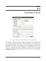
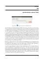
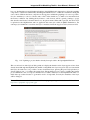
OPENQUAKE PLATFORM CONNECTION SETTINGS
Fig. 4.1:
OQ-Platform connection settings
Some of the functionalities provided by the plugin, such as the ability to work with GEM data, require
the interaction between the plugin itself and the OpenQuake Platform (OQ-Platform). The OQ-Platform
is a web-based portal to visualize, explore and share GEM’s datasets, tools and models. In the Platform
Settings dialog displayed in Fig. 4.1, credentials must be inserted to authenticate the user and to allow
the user to log into the OQ-Platform. In the Host field insert the URL of GEM’s production installation
of the OQ-Platform1 or a different installation if you have URL access. If you still haven’t registered to
use the OQ-Platform, you can do so by clicking Register to the OQ-Platform. This will open a new web
browser and a sign up page2 . The checkbox labeled Developer mode (requires restart) can be used to
increase the verbosity of logging. The latter is useful for developers or advanced users because logging
is critical for troubleshooting, but it is not recommended for standard users.
1
2
https://platform.openquake.org
https://platform.openquake.org/account/signup/
6
CHAPTER
FIVE
LOADING SOCIOECONOMIC INDICATORS FROM THE
OPENQUAKE PLATFORM
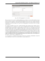
Fig. 5.1:
Socio-economic indicators selection portal
The selection of data comprises an essential step for an assessment of risk from an integrated and holistic
perspective using indicators. The strengths and weaknesses of composite indicators are derived to a great
extent by the quality of the underlying variables. Ideally, variables should be selected based on their
relevance to the phenomenon being measured, analytical soundness, accessibility, and completeness
[NSST08]. Proxy measures for social and economic vulnerability have been provided by the Global
Earthquake Model that have been stringently tested for representativeness, robustness, coverage and
analytical soundness [KBT+14]. These are currently accessible in the IRMT at the national level of
geography (gadm L1). Future software releases will add access to data at gadm level 2 (L2) for a
selection of countries and regions. This will include the eight Andean countries of South America and
countries within Sub-Saharan Africa.
Fig. 5.1. displays the Select Socioeconomic Indicators dialog that was developed to allow users to select
indicators based on a number of factors and filtering mechanisms. A Filters section was developed to
enable users to filter indicators by name, keywords, theme (e.g. Economy) and subtheme (e.g Resource
7
Integrated Risk Modelling Toolkit - User Manual, Release 1.7.5
Distribution and Poverty). The subtheme dropdown menu is automatically populated depending on the
selection of a respective theme. When Get indicators is pressed, a list of filtered indicators is populated
on the left side of the dialog within the Select indicators window. If no filters are set, then the whole
list of indicators available within the database is retrieved and displayed within the Select indicators
window.
From the Select indicators window, it is possible to select one or more indicators by single-clicking them
in the Unselected list on the left. Double-clicking the selected indicator(s) moves them to the Selected
list on the right, and the corresponding data will be downloaded from the OQ-Platform. Another way
to move items to the right, or back to the left, is to use the four central buttons (add the selected items,
remove the selected items, add all, remove all). The Indicator details section displays information about
the last selected indicator: code, short name, longer description, source and aggregation method.
The Select countries dialog contains the list of enumeration types (in this case countries) that socioeconomic data is available for within the database. Countries can be selected from the list in the same
manner that indicators are selected using Select indicators. Once at least one indicator and one country
has been selected, the OK button will be enabled. By pressing the OK button, data will be downloaded
from the OQ-Platform and compiled into a vector shapefile for display and manipulation within QGIS
(another dialog will ask you where to save the shapefile that will be obtained). The layer will contain
features equal to the number of selected countries and will contain all attributes selected as indicators for
the given countries. Additional attributes will include fields containing country ISO codes and country
names. To reduce processing time, detailed country geometries were simplified using ESRI’s Bend Simplify algorithm1 . Bend Simplify removes extraneous bends and small intrusions and extrusions within
an area’s topology without destroying its essential shape.
Fig. 5.2: Layer attribute table
Fig. 5.2 shows the attribute table of a sample vector layer compiled and downloaded within the IRMT.
Note: For some countries the values of indicators might be unavailable (displayed in the attribute table
as NULL).
When the tool downloads the socioeconomic data, a project definition is automatically built taking into
account how the data was organized in the socioeconomic database. At the country level data was
grouped together by theme meaning that indicators belonging to the same theme will be grouped together in a hierarchical structure. This structure considers: 1) vulnerable populations; 2) economies; 3)
education; 4) infrastructure; 5) health; 6) governance and institutional capacities; and 7) the environment.
1
http://resources.arcgis.com/en/help/main/10.1/index.html#//007000000010000000
8
CHAPTER
SIX
DOWNLOADING A PROJECT FROM THE OPENQUAKE PLATFORM
Fig. 6.1:
Downloading a project from the OpenQuake Platform
An additional option to access data is by downloading projects shared by others on the OQ-Platform.
By clicking the Download project from the OpenQuake Platform, the above dialog is opened (Fig. 6.1).
Here, a list of available projects is displayed. The list will contain the titles of projects for which the user
has been granted editing privileges (their own projects or those shared with them by other users). When a
project is selected from the list, its title, abstract, bounding box and keywords are displayed in the lower
textbox that is utilized to delineate important attributes of the project’s definition. The label directly
above the textbox displays an ID that uniquely identifies the layer used in the OpenQuake-platform.
9
Integrated Risk Modelling Toolkit - User Manual, Release 1.7.5
By pressing OK, the layer will be downloaded into the QGIS. Prior to downloading, the layer will first
have to be saved as a new shapefile locally by navigating to a folder in which the shapefile is to be
saved. If the associated project only contains one project definition, it will be automatically be selected
and downloaded. Otherwise, the project definition manager will open (see Project definitions manager)
allowing the user to choose one of the available project definitions. Once a project definition is selected,
the composite indicators delineated within the project definition are re-calculated, and the layer is styled
and rendered accordingly. This process may take some time, depending on the complexity of the project.
10
CHAPTER
SEVEN
TRANSFORMING ATTRIBUTES
Fig. 7.1:
Variable transformation and batch transformation functionality
Once variables are selected, they should be standardized or normalized before they are aggregated into
composite indicators. This is because variables are delineated in a number of statistical units that could
easily consist of incommensurate ranges or scales. Variables are standardized to avoid problems inherent
when mixing measurement units, and normalization is employed to avoid having extreme values dominate an indicator, and to partially correct for data quality problems. The QGIS platform natively provides
a Field calculator that can be used to update existing fields, or to create new ones, in order to perform
a wide variety of mathematical operations for the standardization/transformation of data. In addition,
the IRMT provides a number of transformation functions found in popular statistical and mathematical
modelling packages (Table 7.1).
11
Integrated Risk Modelling Toolkit - User Manual, Release 1.7.5
Table 7.1: Selection of transformation functions with equations found in the
IRMT.
Standardization (or Z-scores)
𝑍(𝑥𝑖 ) =
Min-Max
𝑀 (𝑥𝑖 ) =
Logistig Sigmoid
𝑆(𝑥𝑖 ) =
Simple Quadratic
𝑄(𝑥𝑖 ) =
𝑥𝑖 −𝜇𝑥
𝜎𝑥
(𝜇𝑥 = 𝑚𝑒𝑎𝑛 𝜎𝑥 = 𝑠𝑡𝑑𝑑𝑒𝑣)
𝑥𝑖 −min𝑖∈{1,...,𝑛} (𝑥𝑖 )
max𝑖∈{1,...,𝑛} (𝑥𝑖 )−min𝑖∈{1,...,𝑛} (𝑥𝑖 )
1
1+𝑒−𝑥𝑖
𝑥2
max𝑖∈{1,...,𝑛} (𝑥𝑖 )
These include:
1. Data Ranking is the simplest standardization technique. Ranking is not affected by outliers and
allows the performance of enumeration units to be benchmarked over time in terms of their relative
positions (rankings).
2. Z-scores (or normalization) is the most common standardization technique. A Z-score converts
indicators to a common scale with a mean of zero and standard deviation of one. Indicators with
outliers that are extreme values may have a greater effect on the composite indicator. The latter
may not be desirable if the intention is to support compensability where a deficit in one variable
can be offset (or compensated) by a surplus in another.
3. Min-Max Transformation is a type of transformation that rescales variables into an identical
range between 0 and 1. Extreme values/or outliers could distort the transformed risk indicator.
However, the MIN-MAX transformation can widen a range of indicators lying within a small
interval, increasing the effect of the variable on the composite indicator more than the Z-scores.
4. Log10 is one of a class of logarithmic transformations that include natural log, log2, log3, log4,
etc. Within the current plugin, we offer functionality for log10 only, yet these transformations
are possible within the advanced field calculator. A logarithm of any negative number or zero is
undefined. It is not possible to log transform values within the plugin if the data contains negative
values or a zero. For values of zero, the tool will warn users and suggest that a 1.0 constant be
added to move the minimum value of the distribution.
5. Sigmoid function is a transformation function having an S shape (sigmoid curve). A Sigmoid
function is used to transform values on (−∞, ∞) into numbers on (0, 1). The Sigmoid function
is often utilized because the transformation is relative to a convergence upon an upper limit as
defined by the S-curve. The IRMT utilizes a simple sigmoid function as well as its inverse. The
Inverse of the Sigmoid function is a logit function which transfers variables on (0, 1) into a new
variable on (−∞, ∞).
6. Quadratic or U-shaped functions are the product of a polynomial equation of degree 2. In
a quadratic function, the variable is always squared resulting in a parabola or U-shaped curve.
The IRMT offers an increasing or decreasing variant of the quadratic equation for horizontal
translations and the respective inverses of the two for vertical translations.
Note: It may be desirable to visualize the results of the application of transformation functions to
data. Although not feasible within the plugin at this point, we intend to build data plotting and curve
manipulating functionalities into future versions of the toolkit.
The Transform attribute dialog (Fig. 7.1) was designed to be quite straightforward. The user is required
to select one or more numeric fields (variables) available in the active layer. For the selection to be
completed, the user must move the variables (either one at a time, or in a batch) to the Selected variables
window on the right side of the interface. The user must then select the function necessary to transform
the selected variables. For some functions, more than one variant is available. For functions that have
12
Integrated Risk Modelling Toolkit - User Manual, Release 1.7.5
an implementation of an inverse transformation, the Inverse checkbox will be enabled to allow users to
invert the outcome of the transformation.
The New field(s) section contains two checkboxes and a text field. If the first checkbox Overwrite the
field(s) is selected, the original values of the transformed fields will be overwritten by the results of the
calculations; otherwise, a new field for each transformed variable will be created to store the results.
In situations in which a user may desire to transform variables one at a time rather than using a batch
transformation process, it is possible for the user to name each respective new field (editing the default
one proposed by the tool). Otherwise, the names of the new fields will be automatically assigned using
the following convention: if the original attribute is named ORIGINALNA, the name of the transformed
attribute becomes _ORIGINALN (prepending “_” and truncating to 10 characters which is the maximum
length permitted for field names in shapefiles).
If the checkbox Let all project definitions utilize transformed values is checked, all the project definitions associated with the active layer will reference the transformed fields instead of the original ones.
Otherwise, they will keep the links to the original selected attributes. In most cases it is recommended to
keep this checkbox checked. This automatic update of field references simplifies the workflow because
it avoids the need to manually remove the original nodes from the weighting and aggregation tree (discussed in detail in Weighting data and calculating indices) in order to add the transformed nodes and
to set again the nodes’ weights. In other words, if a project was developed by weighting and aggregating untransformed indicators, this functionality allows for variables used in the project definition to be
replaced on-the-fly (and automatically) by transformed variables. This saves the user from having to
augment the model manually.
By clicking the Advanced Calculator button, the native QGIS field calculator is opened. Please refer
to the code documentation for the detailed description of all the agorithms and variants provided by the
IRMT.
13
CHAPTER
EIGHT
PROJECT DEFINITIONS MANAGER
Fig. 8.1:
Project definitions manager
The Project Definitions Manager is a module that was developed to allow users to create multiple models
that can be accessed with a click of a button using a single layer. Each project definition (see Definitions)
can define a different model structure, weighting and aggregation scheme, and variable selections among
data available in the underlying layer. It allows users to seamlessly toggle through various integrated risk
assessment projects without having to refer to different QGIS projects or different layers containing data
for a given area or areas, and without having to re-symbolize data to compare results of assessments
using different methodological parameters. The Project definitions manager was developed around a
dialog window that enables users to edit the current project definition, to switch from the current project
definition to a different one, to add a new project definition, or to clone an existing project definition.
While contributing to the Title and Description textbox of the project definitions manager, the Raw
textual representation is updated accordingly.
14
Integrated Risk Modelling Toolkit - User Manual, Release 1.7.5
Warning: It is not recommended for users to edit the parameters directly inside the raw textual
representation portion of the project definition manager, although it is not forbidden. This especially
applies to variable names (field names) and sub-indicators (also field names) defined by nodes within
the weighting and aggregation tree (see Weighting data and calculating indices). Manual adjustments
can be useful in some corner cases, by experienced users, but manual adjustments can cause the
toolkit to behave unexpectedly and can cause shapefiles to behave unexpectedly. Users performing
these adjustments are at risk of compromise their data.
The + button at the right of the dropdown menu can be used to associate the current layer with a new
project definition. By clicking it, a new basic project definition is created and the user is invited to provide the new project definition with a title and, possibly, a description. The button Make a copy of the
selected project definition, assigns to the active layer within the QGIS a new project definition that is an
exact clone of the selected one. Having two similar project definitions can be useful to easily visualize
how the output of a project is changed based on updated variable selections, weighting, and aggregation
schemes. This visualization is possible because a simple click is sufficient to switch between before
and after project definitions. When OK is pressed, the composite indices are re-calculated accordingly
with the project definition and the layer is styled as a consequence via a default classification and symbolization that is adjustable within the QGIS. This computation can take some time, depending on the
complexity of the layer.
15
CHAPTER
NINE
WEIGHTING DATA AND CALCULATING INDICES
Fig. 9.1:
Tree chart structure for the development of composite indicators
Central to the construction of composite indicators is the need to meaningfully combine different data
dimensions, and consideration must be given to weighting and aggregation procedures. Most composite
indicators rely on equal weighting largely for simplicity. Equal weighting, however, implies that all
variables within the composite indicator are of equal importance when this may not actually be the case.
The issue of aggregation is similar to the weighting process. Different aggregation rules may be applied depending on the underlying theoretical framework chosen by the user for the modelling process.
Sub-indicators may be summed up (linear aggregation) for instance, multiplied, or geometrically aggregated to correct for compensability (i.e., the possibility of offsetting a deficit in some dimension with
an outstanding performance in another). Each technique has specific consequences, implies different
assumptions, and could ignore or incorporate weights.
The Weight data and calculate indices widget (Fig. 9.1) is the key module of the IMRT. It contains
the model building functionality of the IRMT, and it is used to create, edit, and manage composite
indicator(s) and integrated risk model development. It provides users with an intuitive way to develop
composite models by building and editing the selected project definition through the use of a dynamic
graphical interface that was developed explicitly to guide the construction of composite indicators in a
manner that is simple, visual, and straight-forward. The latter is accomplished through a window that
16
Integrated Risk Modelling Toolkit - User Manual, Release 1.7.5
embeds a dynamic model builder that takes the form of a tree chart (see Fig. 9.1). This structure (or
weighting and aggregation tree) defines a workflow that strings together sequences of steps to describe
how variables are combined together to obtain the composite indices.
Fig. 9.2: Composite indicator types
Currently, the IRMT supports the development of two composite model types: a) deductive and, b) hierarchical (Fig. 9.2 1 ). Deductive models typically contain fewer than ten indicators that are normalized
and aggregated to create an index. Hierarchical models typically employ ten to twenty indicators that
are separated into groups (sub-indices) that share the same underlying dimension of a concept (in this
case socio-economic parameters of earthquake risk such as population, economy, infrastructure, education, and governance). Individual indicators are aggregated into sub-indices (e.g., population, economy,
etc.), and the sub-indices are aggregated to form a final composite index (e.g., social vulnerability or
integrated risk index). The tree structure of the Weight data and calculate indices widget encourages the
development of hierarchical models of integrated risk. The starting point is a root node that corresponds
to the development of a hierarchical model that can be: 1) an Integrated Risk Index (IRI) which is a
function of the aggregation of a Social Vulnerability Index (SVI) and a Risk Index (RI); or 2) a Social
Vulnerability Index (SVI) that is the result of the aggregation of various sub-indicators defined by the
user (e.g., Economy, Education, and Environment as shown within Fig. 9.1). The tree can be modified
dynamically by adding or removing nodes, inverting variables, setting a weight to each variable or node
and choosing the operators to be used to combine variables together.
Whenever Update or Update and close are clicked, the project definition is updated and the composite
indices are re-calculated. As a consequence, the map is rendered and styled accordingly. This allows the
user to have an immediate feedback on how the map changes depending on how the project definition is
1
Adapted from [TAT12]
17
Integrated Risk Modelling Toolkit - User Manual, Release 1.7.5
set. Such automatic re-calculations and rendering can take some time, depending on the complexity of
the project and number of enumeration units analysed. Sometimes it is more convenient to disable the
on-the-fly calculations while changing the project’s structure, and enable it again once the project has
been built. In order to do so, it is sufficient to toggle the Run calculations on-the-fly checkbox.
The main functional elements of the weighting and aggregation tree are discussed in the subsections
below.
9.1 Adding a node
Individual nodes correspond to aggregated composite indicators within the weighting and aggregation
tree. To add a node (i.e., a composite sub-indicator) within the tree, it is possible to begin by leftclicking on the default node (i.e., SVI). Clicking on the default SVI node allows the addition of multiple
new sub-indicators, each with its own user-provided name.
Note: It is not possible to add nodes stemming from the IRI.
When a newly created node is clicked, a new dialog is initiated to give users the option to select the
variables available in the layer (and not already used in the node) to populate the sub-indicator being
under construction.
Note: The SVI can be calculated if each socioeconomic sub-indicator has at least one variable.
In order to add an indicator to one of the socioeconomic sub-indicators, you can click on the corresponding node. When adding an indicator to the RI, or to one of the socioeconomic sub-indicators, the
description of the node will be automatically set to be equal to the name of the corresponding layer’s
variable. Users can edit this description, however, by clicking on the text displayed next to the node in
the tree and then by clicking within the corresponding textbox to change the text.
9.2 Removing a node
In order to remove one of the nodes from the tree, users can perform a right-click on that node. A popup
dialog window will ask you to confirm if you really intend to delete the node and all of its children (the
lower level nodes connected to it).
Note: Removing a node from the tree will not delete the corresponding field from the layer.
9.3 Setting the operators to be used to aggregate variables
On the right of each node, the tree indicates the name of the operator to be used to combine (or aggregate)
the variables making up the node. By clicking on the operator’s name, a dialog to set weights and
operators is opened. The same happens when clicking on the name of one of the children nodes. The
operator can be chosen from a dropdown menu. Some operators (e.g., Weighted sum) take into account
the weights applied to the child nodes. Other operators (e.g., Average (ignore weights)) do not take
into account weights. When the chosen operator is one of the latter, the child nodes will be rendered
on the graphical display all with the same radius and their weights will not be rendered (see Fig. 9.1
9.1. Adding a node
18
Integrated Risk Modelling Toolkit - User Manual, Release 1.7.5
for a demonstration of how the radius of nodes corresponds with the respective weights of variables).
Otherwise, the radius of a node is proportional to its weight, and the weight is rendered next to the node.
9.4 Setting weights
Central to the construction of composite indicators in the need to combine data which implies decisions
on weighting. The dialog to set weights is opened in the same way as described in Setting the operators
to be used to aggregate variables. Several weighting techniques are available, and some make use of
statistical models. For the IRMT we implemented a simple solution to weighting that is often based
on the results of participatory approaches. A weight can be edited manually by clicking on its value
and overwriting it with a new value. A weight can also be edited by clicking on the spinner’s arrows to
increase or decrease the weight. By clicking Update, the weights will be re-calculated in order to make
them sum to 1. In other words, if you have 3 variables and you set their weights to 1, 2 and 5 and you
press Update, the weights will be re-calculated to be respectively 0.125, 0.250 and 0.625, keeping the
same proportion between each other, and summing to 1.
9.5 Inverting a variable
The dialog to invert variables is opened in the same way as described in Setting the operators to be used
to aggregate variables. If a variable contributes in a negative way to the composite indicator (e.g., a
higher education corresponding to a lower social vulnerability), it is possible to indicate such an inverse
relationship by pressing the Invert button next to the variable name. The effect on a composite indicator
in response to this decision process and setting is that each value of an inverted variable will be to
multiplied by -1 each time the variable is used in a calculation.
Note: Please note that the layer’s field will keep holding the original value of the variable, and that the
inversion will be performed on-the-fly for the purpose of the calculation.
9.6 Assigning a new name to a variable
The dialog to assign a new name to a variable is also opened in the same way as described in Setting
the operators to be used to aggregate variables. By clicking on the variable’s name, a popup dialog
asks users to insert the new name. The project definition will be updated accordingly, linking the layer’s
fieldname with the modified description.
9.7 Styling the layer by a chosen field
The dropdown menu entitled Style layer by on the bottom of the Set weights and operators module can
be used to choose fields within a layer, i.e., fields other than those delineated within the project definition
to be symbolized, allowing all fields in a layer to be to be symbolized on-the-fly. This can be useful, for
instance, to map the values calculated for different sub-indicators, or even individual variables if they
are of interest. By default, the selection is blank. In the default case, the tool will adopt the following
convention: 1) if the IRI can be computed, then the layer will be symbolized according to it; 2) otherwise,
if the SVI can be computed, then it will be used as the default case for symbolization in the absence of
IRI; 3) otherwise, the convention will apply with respect to the RI; and 4) if none of main sub-indicators
9.4. Setting weights
19
Integrated Risk Modelling Toolkit - User Manual, Release 1.7.5
can be calculated, then the layer will not be re-styled unless the user uses the dropdown menu to specify
a specific symbolization field.
9.7. Styling the layer by a chosen field
20
CHAPTER
TEN
AGGREGATING LOSS BY ZONE
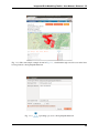
Fig. 10.1:
Aggregate loss by zone data import tool
The development of an integrated risk model (IRI) arises from the convolution of two main components: 1) estimations of physical risk (RI), and 2) a social vulnerability index (SVI). The convolution
of earthquake physical risk and social vulnerability parameters can be accomplished by, first, importing risk assessments from OpenQuake (or some other source) using the toolkit’s risk import tool (Fig.
10.1). To import data, users can click the Aggregate loss by zone button that prompts a dialog window
to open. Here, it is possible to select layers containing estimations of physical risk, (Loss layer) or some
other type of risk model, and to combine these with a layer containing zonal geometries of the study
area (e.g., country borders, district borders) and socioeconomic indicators. The top dropdown menu is
pre-populated with the names of the available vector layers containing point geometries (a native output
of the OQ-Engine), while the second dropdown menu is pre-populated with the names of the available
vector layers containing polygonal geometries. If those menus do not contain the desired layers, it is
possible to click one of the ... buttons, to load another layer from the file system. As soon as a new
layer is loaded, it will be available in the QGIS table of contents and its name will become available and
pre-selected in the corresponding dropdown menu.
Estimations of physical risk can be made available from the OQ-Engine as one or multiple CSV files.
By selecting the file type Loss curves from the OpenQuake-engine, such files become available and can
be (multi)selected. The resulting loss layer will contain a number of attributes equal to the number of
CSV files imported, and each attribute will correspond to a different loss type.
Loss data from the OQ-Engine is rendered as points containing X,Y locational coordinates and the loss
values for the different assets represented at a given location. Once both a loss layer and a zonal layer
have been selected, the above dialog window is opened (Fig. 10.2). In the Loss Layer section of the
dialog window, the user is invited to select one or more attributes from the loss layer. This selection
is because the toolkit will calculate the sum and average values for each of the zonal layer’s features,
and it will add those statistics to the zonal layer as new attributes. Within the layer’s attribute table, a
subsequent attribute will be added to display the count of loss points that are found inside the boundaries
of each feature. The latter can be useful for troubleshooting.
21
Integrated Risk Modelling Toolkit - User Manual, Release 1.7.5
Fig. 10.2: Zonal aggregation of loss values
The aggregation by zone can be obtained in different ways. If the user is aware that both the loss layer
and the zonal layer contain a common attribute that indicates the id of the zone to which each feature
belongs, then it is sufficient to select this common attribute both for the loss layer and the zonal layer,
and let the tool perform a simple join. In this case, the aggregation is fast because it does not require
spatial analysis.
If a common zonal ID does not exist, a spatial join using zonal geometries may be utilized. This is
accomplished, first, by selecting Use zonal geometries within the Zone ID attribute name dropdown
menu that contains also the names of all the attributes of the loss layer. As a consequence, the tool will
perform a spatial search to detect to which zone each of the loss points belongs. The Zone ID attribute
name in the zonal layer is the attribute that uniquely identifies each of the zones. If the user is not sure
if features are uniquely identified by any of the available attributes in the zonal layer, then it is possible
to select the additional item Add field with unique zone id. As a consequence of this choice, the tool will
produce an additional attribute in the corresponding layer, and it will set the values of that attribute to be
equal to the unique id of the corresponding feature. Then the new attribute will be used as unique id of
the feature, to perform the loss aggregation by zone.
As a subsequent step, earthquake risk data imported into the tool should be standardized to render the
data commensurate to the socioeconomic indicators created within the tool.
22
CHAPTER
ELEVEN
UPLOADING A PROJECT TO THE OPENQUAKE PLATFORM
Fig. 11.1: Simplified Integrated Risk analysis as it is seen inside QGIS right before the project is
uploaded to the OpenQuake Platform
Once an integrated risk model is complete, and the user is satisfied with results such as those obtained
for the example displayed in Fig. 11.1, it is possible to upload projects through the OQ-Platform.
Projects are uploaded in order to share them with the wider earthquake risk assessment, earthquake risk
reduction, GIS communities, etc. Uploading to the OQ-Platform also supports the ability to visualize
models using advanced visualization tools and the mapping of the data over the web. In addition, sharing
the models on the OQ-Platform allows users that are not QGIS savvy to dynamically interact with the
data. The mapping and visualization over the web is accomplished using the OQ-Platform (Fig. 11.2)
and the Social Vulnerability and Integrated Risk Viewer (see the web application1 and the corresponding
documentation2 ).
To upload a project to the OQ-Platform, click Upload project to the OpenQuake Platform. This will
result in the opening of a dialog window in which, depending on the context, the window will look like
those delineated in Fig. 11.3 or Fig. 11.4. The former will be displayed if the current project has never
been uploaded to the OQ-Platform. In such cases, the user is invited to provide a project title that will
become the title of the layer that will be created on the Platform. A second field will contain the abstract,
where the user can provide a general description of the project.
Note: In order to be able to correctly utilize the advanced visualization tools found on the OQ-Platform,
the selection of a Zone labels field is required (see Fig. 11.3).
The user must designate the Zone labels field within their dataset. The latter is a field containing unique
labels (or identifiers) whether these are individual country names, district names, or census block num1
2
https://platform.openquake.org/irv_viewer/
http://www.globalquakemodel.org/openquake/support/documentation/platform/irv/
23
Integrated Risk Modelling Toolkit - User Manual, Release 1.7.5
Fig. 11.2: The same simple example shown in Fig. 11.1, visualized through a web browser after it has
been uploaded to the OpenQuake Platform
Fig. 11.3:
Uploading a project to the OpenQuake Platform
24
Integrated Risk Modelling Toolkit - User Manual, Release 1.7.5
bers, etc. Delineating a zone field when uploading to the OQ-Platform is imperative to allow the graphing
components of the Social Vulnerability and Integrated Risk Viewer to render the visualization using the
zone’s labels. Without the latter, comparisons among places within the graphing tools are not possible.
It is also mandatory to choose a license and to click on the checkbox to confirm to be informed about
the license conditions. By clicking the Info button, a web browser will be opened, pointing to a page
that describes the license selected in the License dropdown menu. When OK is pressed, the active layer
is uploaded to the OQ-Platform and it is applied in the same style visible in QGIS. Furthermore, the
current project definition is saved into the layer’s metadata, inside the Supplemental information field.
Fig. 11.4: Updating a project that has already been uploaded to the OpenQuake Platform
This second version of the Upload dialog window is displayed when the active layer appears to have been
already shared through the OQ-Platform (the ID of a OQ-Platform’s layer was previously associated with
this layer). In such cases, it is possible to create a brand new layer, ignoring the previously uploaded (or
downloaded) project, or to update the current layer. The updating process consists of adding the current
project definition to the set of project definitions associated to that layer on the OQ-Platform. This is a
much faster procedure because no geometries need to be uploaded, and only the metadata of the layer
will be changed.
Note: This documentation is distributed within the plugin’s package and it is also available online at
http://docs.openquake.org/oq-irmt-qgis/
25
BIBLIOGRAPHY
[SCP+14] Silva, V., Crowley, H., Pagani, M., Monelli, D., and Pinho, R., 2014. Development of the
OpenQuake engine, the Global Earthquake Model’s open-source software for seismic risk assessment. Natural Hazards 72(3), 1409-1427.
[NSST05] Nardo, M., Saisana, M., Saltelli, A. and Tarantola, S. 2005. Tools for composite indicators
Building. Ispara, Italy: Joint Research Center of the European Commission.
[NSST08] Nardo, M., Saisana, M., Saltelli, A. and Tarantola, S. 2008. Handbook on constructing composite indicators: Methodology and user guide. Paris, France: OECD Publishing.
[ESRI98] ESRI Shapefile Technical Description, Environmental Systems Research Institute, Redlands,
C.A.
[KBT+14] Khazai B, Burton C.G., Tormene, P., Power, C., Bernasocchi, M., Daniell, J., and Wyss, B.
(2014) Integrated Risk Modelling Toolkit and Database for Earthquake Risk Assessment. Proceedings of the Second European Conference on Earthquake Engineering and Seismology, European
Association of Earthquake Engineering and European Seismological Commission, Istanbul, Turkey.
[TAT12] Tate, E.C. 2012. Social vulnerability indices: a comparative assessment using uncertainty and
sensitivity analysis, Natural Hazards, 63(2): 325-347
26