1
Copyright Warning & Restrictions
The copyright law of the United States (Title 17, United
States Code) governs the making of photocopies or other
reproductions of copyrighted material.
Under certain conditions specified in the law, libraries and
archives are authorized to furnish a photocopy or other
reproduction. One of these specified conditions is that the
photocopy or reproduction is not to be “used for any
purpose other than private study, scholarship, or research.”
If a, user makes a request for, or later uses, a photocopy or
reproduction for purposes in excess of “fair use” that user
may be liable for copyright infringement,
This institution reserves the right to refuse to accept a
copying order if, in its judgment, fulfillment of the order
would involve violation of copyright law.
Please Note: The author retains the copyright while the
New Jersey Institute of Technology reserves the right to
distribute this thesis or dissertation
Printing note: If you do not wish to print this page, then select
“Pages from: first page # to: last page #” on the print dialog screen
The Van Houten library has removed some of the
personal information and all signatures from the
approval page and biographical sketches of theses
and dissertations in order to protect the identity of
NJIT graduates and faculty.
ABSTRACT
FLEXIBLE MANUFACTURING SYSTEM UTILIZING COMPUTER
INTEGRATED CONTROL AND MODELING
by
Yahia Mohammed Al-Smadi
In today's fast-automated production, Flexible Manufacturing Systems (FMS) play a very
important role by processing a variety of different types of workpieces simultaneously.
This study provides valuable information about existing FMS workcells and brings to
light a unique concept called Programmable Automation.
Another integrated concept of programmable automation that is discussed is the
use of two feasibility approaches towards modeling and controlling FMS operations; the
most commonly used is programmable logic controllers (PLC), and the other one, which
has not yet implemented in many industrial applications is Petri Net controllers (PN).
This latter method is a unique powerful technique to study and analyze any production
line or any facility, and it can be used in many other applications of automatic control.
Programmable Automation uses a processor in conventional metal working
machines to perform certain tasks through program instructions. Drilling, milling and
chamfering machines are good examples for such automation.
Keeping the above issues in concern; this research focuses on other core
components that are used in the FMS workcell at New Jersey Institute of Technology,
such as; industrial robots, material handling system and finally computer vision.
FLEXIBLE MANUFACTURING SYSTEM UTILIZING COMPUTER
INTEGRATED CONTROL AND MODELING
by
Yahia Mohammed Al-Smadi
A Thesis
Submitted to the Faculty of
New Jersey Institute of Technology
In Partial Fulfillment of the Requirements for the Degree of
Master of Science in Manufacturing Systems Engineering
Department of Industrial and Manufacturing Engineering
May 2002
APPROVAL PAGE
FLEXIBLE MANUFACTURING SYSTEM UTILIZING COMPUTER
INTEGRATED CONTROL AND MODELING
Yahia Mohammed Al-Smadi
Dr. Kevin J. McDermott, Thesis Advisor
Associate Professor of Industrial and Manufacturing Engineering,
Director of Cad/Cam Robotics Consortium, NJIT
Date
Dr. Athanassios K. Bladikas. Committee Member
Associate Professor of Industrial and Manufacturing Engineering
Chair of Industrial and Manufacturing Engineering Department, NJIT
Date
1-1
Dr. George H. Abdou, Committee Member
Associate Professor of Industrial and Manufacturing Engineering,
Associate Chair & Program Director: Industrial Engineering Programs, NJIT
Date
BIOGRAPHICAL SKETCH
Author :
Yahia Mohammed Al-Smadi
Degree:
Master of Science
Date:
May 2002
Undergraduate and Graduate Education
•
Master of Science in Manufacturing Systems Engineering
New Jersey Institute of Technology, Newark, NJ, 2002
•
Bachelor of Science in Mechanical Engineering
Jordan University of Science and Technology, Irbid, Jordan, 1999
Major:
Manufacturing Systems Engineering
This thesis is dedicated to my
beloved parents and family members
v
ACKNOWLEDGMENT
I would like to express my sincere gratitude to Dr. Kevin J. McDermott for his invaluable
guidance, support and encouragement throughout the research.
Special thanks to Dr. Athanassios K. Bladikas and Dr. George Abdou for actively
participating as members of the committee.
I would like to thank Dr. R. Kane and Ms. C. Gonzalez for their help and guidance to
write this thesis
Thanks to Mr. Abuibraheem Choudry and Mr. Sherif Mandi for their help and
constructive criticism
Thanks are also due to the Robotics Training Lab, New Jersey Institute of Technology,
where I gained most of my experience in the robotics and PLC fields.
vi
TABLE OF CONTENTS
Page
Chapter
1 FLEXIBLE MANUFACTURING SYSTEMS 1.1 Introduction
1
1
1.2 Data Flow of FMS 2
1.3 Hierarchical Structure of an FMS Control System
4
1.4 Advantages of FMS
5
1.5 Components of FMS 6
1.5.1 Four Processing Stations
7
1.5.2 Robots 10
1.5.3 Material Handling System and Storage 12
1.5.4 Logic Controllers PLC. GE Series Cell Controller 13
1.6 FMS Layout Configuration 14
1.7 Product Cycle 14
16
2 COMPUTER NUMERICAL CONTROL 2.1 Introduction 16
2.2 CNC Machine Classification 17
2.2.1 Mechanical Systems 18
2.2.2 Control System 22
2.2.3 Coordinate System 24
2.2.4 Motion Control System 25
2.2.5 Number of Axes 27
2.2.6 Control Loop System 28
2.3 Numerical Control/Computer Numerical Control/
Direct Numerical Control NC/CNC/DNC 29
2.3.1 Digital Computer for NC 29
2.3.2 Direct Numerical Control (DNC) 30
2.3.3 Distributed Numerical Control (DNC/CNC) 31
32
2.4 NC Part Programming 33
2.4.1 Manual Data Input — MDI vii
TABLE OF CONTENTS
(Continued)
Chapter
Page
2.4.2 Manual Part Programming 33
2.4.3 Computer-Assisted Part Programming 34
2.4.4 NC Part Programming Using CAD/CAM 34
2.5 Data Preparation for Numerical Control 35
2.6 Case Study for NJIT FMS 36
3 INDUSTRIAL ROBOTS AND INTERFACE WITH CAD SYSTEM 38
3.1 Introduction 38
3.2 Programming Techniques 39
3.3 Robot Software 39
3.4 Robot Anatomy 41
3.5 WorkSpace3 44
3.5.1 Features 44
3.5.2 Specifications 45
3.5.3 Applications 45
3.6 Case Study Sample Program for Drilling Operation done by NJIT FMS 4 COMPUTER VISION INSPECTION 46
50
4.1 Introduction 50
4.2 Operations of Computer Vision 51
4.2.1 Image Acquisition and Digitization 52
4.2.2 Image Processing and Analysis 53
4.2.3 Interpretation 54
4.3 The Itran IVS Computer Vision System 56
4.3.1 Obtaining an Image 57
4.3.2 Area Tools 57
4.3.3 Screen Messages, RS232 Outputs and Discrete I/O 59
4.4 The FS 11 — Feature Sensor 59
viii
TABLE OF CONTENTS
(Continued)
Page
Chapter
4.5 Inspection Method 62
4.6 Project Description 64
5 PROGRAMMABLE LOGIC CONTROLLERS 65
5.1 Introduction 65
5.2 PLC Devices 66
5.3 PLC Components 67
5.4 PLC Computer Functions 68
5.5 Advantages of PLC 68
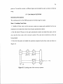
5.6 Basic Logic Gates used in PLC AND, OR, and NOT 68
5.7 Case Study NJIT FMS 71
6 PETRI NET MODELING AND SIMULATION 74
6.1 Introduction 74
6.2 Petri Net Definitions 75
6.3 Petri Nets 76
6.3.1 Mathematical Models 76
6.3.2 Applications 79
6.4 Modeling Methods 79
6.5 Case Study Modeling and Analysis of PN for NJIT FMS 81
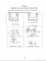
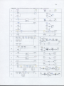
6.5.1 Description and Modeling 81
6.5.2 Analysis 90
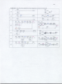
6.6 PN Vs PLC 90
6.7 Analysis of Ladder Logic (LLD) Diagram and PN 91
93
7 CONCLUSIONS ix
TABLE OF CONTENTS
(Continued)
Page
Chapter
APPENDIX A
FMS DRAWINGS SHOW NJIT FMS 94
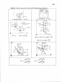
APPENDIX B
FORMULAS THAT CAN BE USED FOR CNC
PROGRAMMING 99
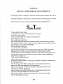
APPENDIX C
DRILLING AND MILLING OPERATIONS PROGRAM 102
APPENDIX D
CREATING A SIMPLE ROBOT 104
APPENDIX E
INPUT AND OUTPUT PORTS USED IN PLC TO
CONTROL THE FMS 106
APPENDIX F
DESCRIPTION FOR EACH PORT AND SEQUENCE
USED IN PLC 110
APPENDIX G
PLC LADDER LOGIC DIAGRAM FOR NJIT FMS 117
APPENDIX H
PN PRESENTATION FOR LLD 120
REFERENCES
124
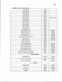
LIST OF TABLES
Page
Table
6
1.1
Comparison Between FMS and Conventional System Performance 2.1
Classification for Number of Axes of CNC Machines 27
2.2
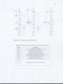
Olivetti Machining Center Program "Chamfering Operation" 36
3.1
Points Coordinate with Joints Motions of the Robot 46
5.1
Input and Output PLC Devices 66
5.3
Basic Logic Gates used in Logical Controller 69
6.1
Reachability Tree for the Figure 6.2 79
6.2
Manufacturing Processes and Their Applications by PN 80
6.3
Places (Events) and Transitions for Material Handling System 82
6.4
Reachability Tree of PN Modeling for Material Handling System 83
6.5
Places (Events) and Transitions for Milling Machine,
GE P-50 Robot, Vision System and Part Presentation Station (Feeder) 85
Reachability Tree of PN Modeling for CNC Milling Machine,
GE P-50 Robot, Vision System, and Part Feeder 85
6.7
Places (Events) and Transitions for Drilling Station 86
6.8
Reachability Tree of PN Modeling for Drilling Station 86
6.9
Places (Events) and Transitions for Chamfering Station 87
6.10
Reachability Tree of PN Modeling for Chamfering Station,
GMF MI Robot, and a 100-Tool crib 88
6.11
Comparison of PN and LLD 92
B.1
Formulas Used for CNC Programming 99
C.1
Drilling and Milling Program 102
E.1
Input List 106
E.2
Output List 108
F.1
Sequences Description for PLC Control Program 110
H.1
Petri Net Presentations for the Sequences of LLD 120
6.6
xi
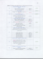
LIST OF FIGURES
Page
Figure
1.1
Data flow of FMS 3
1.2
Hierarchic structure of FMS 4
1.3
Functions for hierarchical structure of FMS 5
1.4
FMS components 7
1.5
NASA II CNC milling machine 8
1.6
Olivetti Machining Center 8
1.7
IBM 7535 Robot
9
1.8
ITRAN vision system 9
1.9
IBM 7535 Robot 10
1.10
General Electric P-50 robot 11
1.11
GMF M1 robot 11
1.12
Cartrac material handling system 12
1.13
Operation of cart on track conveyor 13
1.14
Control system used in NJIT FMS 13
1.15
NJIT FMS layout 14
2.1
Classification of CNC machine 18
2.2
Servomotor 19
2.3
(a) Resolver, (b) Synchros, (c) Inductive linear scales,
(d) Binary encoders, and (e) Laser inferometer 20
2.4
B al I screw 21
2.5
Mounting Ballnuts and Ballscrews; (a) conventional screw
(b,c) Ballscrew 21
2.6
Geometrical properties for the tool 22
2.7
Tools, which are used in (a) NASA II milling machine
(b) Drilling operation 22
2.8
Configuration of CNC machine control unit 23
2.9
Schematic diagram that shows all of MCU, DPU, and CLU used
in CNC machine 24
2.10
Visualization for coordinate system 25
2.11
Point to point control system 26
xii
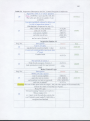
LIST OF FIGURES
(Continued)
Page
Figure
2.12
Straight cut control system 26
2.13
Contouring control system 27
2.14
Classifications of the CNC machines according to their axes 28
2.15
Open loop system 29
2.16
Closed loop system 29
2.17
General configuration of a DNC systems. Connection to MCU is
behind the tape reader 30
2.18a Configuration of DNC: Switching network 31
2.18b Configuration of DNC: LAN configuration 32
2.19
Schematic diagram for part programming methods 33
2.20
Tasks in assisted computer programming 34
2.21
Dimensions of the chamfered block
36
3.1
Process flow from simulation to translation 40
3.2a
Orthogonal joint 42
3.2b
Rotational joint 42
3.2c
Revolving joint 42
3.3a
Rotational joint 43
3.3b
Twisting joint 43
3.4
Linear joint 43
3.5
Rotational axes around X-axis by angle (1) 47
3.6
CAD modeling for GE P-50 robot 49
3.7
CAD modeling for IBM 7535 robot 49
4.1
Basic functions of a machine vision system 52
4.2
Matrix of picture elements, where each element has a high
intensity value corresponding to that portion of the image 53
4.3
Diverse applications for which machine vision has been implemented 55
4.4
FS 11-feature sensor 60
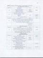
LIST OF FIGURES
(Continued)
Page
Figure
4.5
Tooth brush threshold
64
4.6
Model of the inspected workpart 64
5.1
Examples for input and out devices; (a) Limit switch
(b) Photo detector, (c) Solenoid 66
5.2
Schematic diagram for the PLC controller 67
5.4
An example for LLD programming 70
5.3
Loading state of the conveyor system 71
5.5
Control points 73
6.1
An example of processing which analyzes the mathematical
modeling of a PN 77
6.2
Transition of tokens, which is based on enabling and firing rules 78
6.3
PN modeling for material handling system 82
6.4
Modeling for milling machine, GE P-50 robot, vision system and
Part presentation station (Feeder) 84
6.5
Modeling for drilling station 86
6.6
Modeling for chamfering station 87
6.7
Final Petri net modeling for NJIT FMS cell 89
6.8
Comparison between PN and PLC 91
A.1
NJIT FMS layout SE isometric view 94
A.2
NJIT FMS layout SW isometric view 95
A.3
Schematic diagram for NJIT FMS 96
A.4
Loading/unloading process station 97
A.5
Feeder with parts 98
G.1
LLD diagram used in NJIT FMS cell 119
xiv
CHAPTER 1
FLEXIBLE MANUFACTURING SYSTEMS
1.1 Introduction
Automation is a technology concerned with the application of mechanical, electronic, and
computer based systems used to operate and control production systems. One of the most
important types of automation is flexible automation.
Productivity, cost, quality, and utilization are concepts of concern in most
industries. Flexible manufacturing systems (FMS) can promote the integration of these
concepts and many more which are important to the manufacturer, for example: [27]
•
Flexibility.
•
Group technology.
•
CNC machine tools.
•
Automated material handling between machines.
•
Computer control of machines.
Flexible manufacturing system can be defined as follows:
A Flexible manufacturing system consists of a group of processing stations
(predominantly CNC machine tools), interconnected by means of an automated material
handling and storage system, and controlled by an integrated computer system.[27]
1
2
In addition a flexible manufacturing system can be defined as a computer controlled
configuration of semi-independent work stations and a material handling system designed
to efficiently manufacture more than one part number at low to medium volumes.[32]
In this Chapter, the focus will be on data flow and hierarchy of FMS in Sections
1.2 and 1.3 respectively; components of FMS in Section 1.4; facility layout in Section
1.5; and product cycle in Section 1.6.
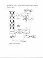
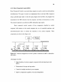
1.2 Data Flow of FMS
It is important to analyze the data flow of the system and to define the function of each
module in the system. The operation of an FMS can be treated as a sequence of events,
which can be done concurrently or in series, whereby one event can trigger the
occurrence of another event.
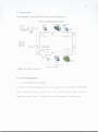
It can be seen from the Figure 1.1 how the data flow between elements
contributes in FMS and also it can be noted that the response of the system is:
✓ Retrieving a new work piece from a storage place
✓ Loading/unloading a work piece a robot
✓ Loading/unloading tools to the machines by robots
✓ Accepting/rejecting machined parts during the inspection stage
✓ Controlling the fixtures and clamps
✓ Controlling the material handling systems such as carts, transporters, and AGV's
✓ Monitoring the conditions of the machine and cutting tool to save the machine
from damage.
3
The system takes care of all procedures until all operations are finished according to the
production schedule.
Figure 1.1 Data flow of FMS.
4
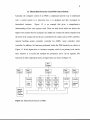
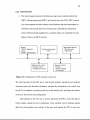
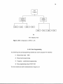
1.3 Hierarchical Structure of an FMS Control System
Typically, the computer control of an FMS is complicated and the way to understand
such a control system is to determine how it is designed and then investigate its
hierarchical structure. Figure 1.2 is an example that gives a comprehensive
understanding of how such systems work. There are three levels which are shown; the
higher level contains the host computer, the middle one contains the client computers and
the lower level contains all the devices controlled by the clients such as CNC controller,
material handling system controller, controller for AS/RS, vision controller, robot
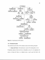
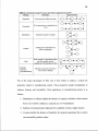
controller. In addition, the functions performed within the FMS hierarchy are shown in
Figure 1.3. In this figure there is a business computer, which is not primary level, and its
basic function is to record and schedule the production and it can be separate. The
functions of other components shown in figure below are shown in Figure 1.3.
Figure 1.2 Hierarchical structure of FMS.
5
Figure 1.3 Functions performed within the FMS hierarchy.
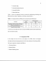
1.4 Advantages of FMS
The advantages resulting from the implementation of FMS have been studied extensively.
They can be summarized as follows:[27&35]
✓ Reduced labor cost.
6
✓ Increased output.
✓ Decreased manufacturing cost.
✓ Increased flexibility.
✓ Reduced lead time.
Table 1.1 shows the comparison between conventional manufacturing technology and
FMS under three criteria's (optimistic, most likely, and pessimistic).
Table 1.1 Comparison Between FMS and Conventional System Performance
Parameter
Percentage of machine time spent without part
Percentage of time when the part is not being
worked on while machine is on
Percentage of manufacturing lead time the part 1I
spends in moving or waiting
Conventional
system
performance
50
FMS performance
Most
Optimistic
Pessimistic
likely
35
20
5
70
35
21
7
95
92.5
90
85
it can be seen in the table above that in all cases the FMS systems has better performance
than conventional systems.
1.5 Components of FMS
In this chapter the focus will be on the analysis of an FMS, which was designed,
developed, fabricated and programmed at the New Jersey Institute of Technology (NJIT).
The major components included in the FMS are:
1. Processing Stations
2. Industrial Robots
3. Material Handling System
7
4. Control System
The components of the NJ IT FMS cell are shown in Figure 1.4.
Flexible Manufacturing System
Figure 1.4 FMS components.
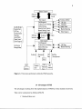
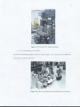
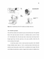
1.5.1 Processing Stations.
• CNC Milling Process Station
The NASA II CNC milling machine shown in Figure 1.5, is driven by DC servomotors
with a closed loop control system with a 3-axis control motion system. It has the
capability to travel in the X, Y, and Z directions, with variations of spindle speed.
8
Figure 1.5 NASA II CNC milling machine.
• CNC Chamfering Process Station.
The Olivetti Machining station, which is shown Figure 1.6, is serviced by a GMF M1
robot and a carousel of 100 tools.
Figure 1.6 Olivetti machining center.Drilling Process Station.
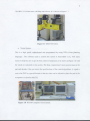
9
The IBM 7535 Robot uses a drilling end effector. It is shown in Figure 1.7.
Figure 1.7 IBM 7535 robot.
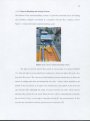
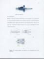
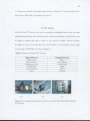
• Vision System
This is a high speed, sophisticated unit programmed by using VPL (vision planning
language). The software used to control this system is SensorEdit v2.1c, with many
menus to help the user to get the best control of inspection. It is shown in Figure 1.8 with
the whole set contained in this system. The Itran computerized vision system inspects the
part and decides if the part meets the specifications of the control algorithms. A signal is
sent to the PLC in a special format so that the robot can be ordered to place the part in the
acceptance or rejection bin.[22]
Figure 1.8 ITRAN Computer vision system.
10
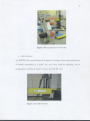
1.5.2 Robots
•
IBM 7535 Robot
This robot is a SCARA type point-to-point robot that is interfaced with the FMS using a
photoelectric sensor fixed to the conveyor system. Its specifications are 5 degrees of
freedom, 4-axis control, payload up to 30 pounds, and repeatability of 0.005" with DC
servo drive. Its configuration is shown in Figure 1.9
Figure 1.9 IBM 7535 robot.
•
General Electric P-50 Robot
The specifications of this robot are 5 degrees of freedom, 5-axis robot, payload of up to
22 pounds and repeatability of 0.008". It is used in the automobile industry for spot
welding applications and is used in this FMS as a material handling robot with hydraulic
drive and a jointed-arm configuration. Figure 1.10 below shows the GE P-50 robot.
11
Figure 1.10 General Electric P-50 robot.
• GMF M1 Robot
The GMF M1 robot specifications are; 6 degrees of freedom, 4-axis robot, payload up to
44 pounds, repeatability of ± 0.005", DC servo drive, used for palletizing, and its
configuration is cylindrical. Figure 1.11 shows the GMF M1 robot.
Figure 1.11 GMF M1 robot.
12
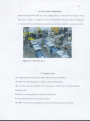
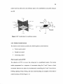
1.5.3 Material Handling and Storage System
The function of the material handling system is to provide convenient access for loading
and unloading workparts and should be compatible with the PLC computer control.
Figure 1.12 shows the Cartrac material handling system
Figure 1.12 Cartrac material handling system.
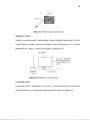
The type of conveyor used in this system is cart-on-track, it is shown in Figure
1.13. The cart rides on a two-railed track contained in a frame that places the track a few
feet above floor level. The carts are not individually powered; instead, they are driven by
means of rotating tubes that run between the two rails. A drive wheel, attached to the
bottom of the cart and set at an angle to the rotating tube, rests against it and drives the
cart forward. Here regulating the angle of contact between the drive wheel and the
spinning tube controls the cart speed. When the drive wheel is perpendicular to the tube,
the cart doesn't move, as the angle is increased toward 45°, the speed increases. In this
way the carts can achieve relatively good accuracies of position.[27]
13
Figure 1.13 Operation of cart-on-track conveyor.
1.5.4 PLC Logic Controller — GE Series Cell Controller
The PLC is the traffic and activities coordinator for the FMS cell. It controls all operations and
functions of the processing stations and the material handling system. It is responsible for carts
flow control, tool and production control and all the other control activities of the workcell.
The subsystem is shown in Figure 1.14.
Figure 1.14 Control system used in NJIT FMS.
14
1.6 FMS Layout Configuration
The layout of the NJIT FMS has a loop configuration, as it was shown in Figure 1.4 and
illustrated in Figure 1.15.additional views for NJIT FMS wrokcell are shown in appendix
A. The parts flow in one direction around the loop with the capability to stop at any station.
Figure 1.15 NJIT FMS layout.
1.7 Product Cycle
One complete product cycle for the FMS workcell operates as follows:
•The GE P-50 robot loads the four conveyor carts with blank parts.
•The conveyor carts are indexed to the four process stations by the Cartrac material
handling system.
•Each process station performs its function concurrently.
•Each part is indexed to the next process station.
•The IBM 7535 robot is programmed to execute the drilling operation on the part
15
•The GMF Ml robot picks the part and loads the Olivetti machining center for the
chamfering operation.
•The GMF M1 robot also loads the tools from the 100-tool crib into the machining
center.
•The GE P-50 robot picks up the part with its vacuum end effecter and places it into the
fixture installed on the CNC milling machine.
•The NASA II CNC milling machine performs the etching of 'NET FMS' on the upper
surface of the part.
•The GE P-50 robot picks up the completed part from the milling machine and loads it
back onto the fixture on the cart.
•The Vision system inspects the completed part to determine the acceptance or rejection
of the part.
•The GE P-50 robot then picks up the completed part and places it in the acceptance or
rejection bin.
CHAPTER 2
COMPUTER NUMERICAL CONTROL
2.1 Introduction
The evolution of this field could not have been possible without the existence and
availability of computers, especially mini or personal computers. The most important
application of computers was in the development of the control operations in the
conventional machines industry such as cutting, welding, lathing, and milling. Computer
use in metalworking machines aids in controlling and performing complex and precise
machining operations at a low cost.
Sections 2.2, and 2.3 contain CNC classifications, Section 2.4 discusses numerical
control (NC), CNC and direct numerical control (DNC), Section 2.5 shows details about
NC part programming and Section 2.6 describes some data used in CNC programming.
Finally there are examples for CNC programming for the case study in NJIT FMS
presented in Section 2.7.
The following terms are used CNC operations:[27]
•
Control Resolution: the capability of machine control unit MCU to divide the
range of a given axis movement into closely spaced points that can be identified by
the controller.
•
Accuracy:.the capacity of MCU to position the worktable at a desired location.
•
Repeatability: the ability of the control system to return to a given location that
was previously programmed into the controller.
•
Mechanical Errors: results from gear backlash, leadscrew play, deflection of
16
17
machine components, and similar inaccuracies in the mechanical positioning system.
2.2 CNC Machine Classification
CNC machines can be classified as shown in Figure 2.1 according to:
✓ Mechanical systems
✓ Control systems
✓ Coordinate system
✓ Motion control
✓ Number of axes
✓ Control loop system
18
Figure 2.1 Classification of CNC machine
2.2.1 Mechanical Systems
The mechanical system used in CNC machines consists of the following vital parts:
• Clamps and Fixture: A Riveted fixture is used in CNC milling table; it is two
Perpendicular plates are fixed with rivets or threaded by screws. It's very important to be
precise in firming the fixture, so a hydraulic motor is used to push the block to the
19
clamps. Generally, the setup of the fixture is the most time consuming process, which
requires tool- making skills to design the proper features for ultimate matching stability.
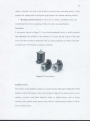
• Mechanical Drive Elements Consist of a servomotor, a feedback system and
recalculating ball screws( consisting of ballscrews and a mounting ballnut).
Servomotor
A servomotor shown in Figure 2.2 is an electromechanical device in which electrical
input determines the position of the armature of a motor and the rotation of the shaft
moves the table forward or backward. They are used extensively in robotics and radiocontrolled cars, CNC machines, airplanes, and boats.
Figure 2.2 Servomotors.
Feedback system
The function of the feedback system is to assure that the table and workpart have been
properly located with respect to the tool. It could be triggered by analog sensors such as
synchros, revolvers, and linear inductive scales, or digital sensors such as binary
encoders, rotary pulsers, linear optical scales, and laser interferometers. Figure 2.3 shows
some example sensors.
20
Figure 2.3 (a) Resolver, (b) Synchros, (c) Inductive linear scales, (d) Binary encoders,
and (e) Laser interferometer.
Ballscrews
A ballscrew shown in Figure 2.4 and 2.5 is a mechanical device that replaces the sliding
friction of leadscrews with the rolling friction of ball bearings placed between the screw
and nut members. A ballscrew performs at very high mechanical efficiency and with
much less energy consumption for a given load. As compared to conventional screw
drives, predictable wear life and smooth quiet operation are also obtained [8].
21
Figure 2.4 Ballscrew.
Mounting Ballnuts
Ballnuts are typically mounted in mating flanges as shown in Figure 2.5, A to restrain the
nut from rotation and translation and are sufficient when loads are axial. If significant
side loads are present, support rails should be used in parallel with the ballscrew. The
longer and the smaller the ballscrew diameter, the greater the possibility of column
loading limitations.[8]
Figure 2.5 Mounting Ballnuts and Ballscrews; (a) conventional screw, (b,c)
Ballscrew.
22
The servomotor is hard mounted on the end of a ground screw that is coupled with a
recirculating ballnut assembly, which allows zero screw backlashes.
• Tools. All parameters associated with the tool such as diameter, length, rpm, and
other geometry features should be saved in CNC control memory. The controller of CNC
machine should have the capability to chose the right tool for that dedicated program.
Tools examples are shown in Figures 2.6 and 2 .7.
Figure 2.7 Tools, which are used in (a) NASA II milling machine, (b) drilling
operation.
23
2.2.2 Control System
• The control system consists of the following major parts; machine control unit
(MCU), data processing unit (DPU), and control loop unit (CLU). MCU consists
of a microcomputer and other related control hardware that store the program of
instructions and execute them by converting each command into mechanical
action of the processing equipment (e.g. machine tools), one command of a time.
Figure 2.8 shows an MCU structure
Figure 2.8 Configuration of CNC machine control unit
The main functions of the DPU are to read the part program, decode the part program
statement, process the decoded information, and pass the information to the control loop
unit (CLU). In addition, it positions each axis of the machine tool, and directs the motion
of the axis, the feed rate and cutting speed.
The functions of the CLU are to receive data from the DPU, convert the data to
control signals, operate the drive mechanisms of the machine, receive feedback signals
about the actual position and velocity of the axes, and instruct the DPU to read new
24
instructions from the part program when the operation has been completed. Figure 2.9
illustrates a schematic diagram of a CNC machine.
Figure 2.9 Schematic diagram that shows the MCU, DPU, and CLU
used in a CNC machine.
2.2.3 Coordinate System
The most basic important programming concept of numerical control is to provide the
mean of locating the tool in relation to the workpiece. Figure 2.11 below shows three
major programming axes, X,Y, and Z, However, there are three more axes; a, b, and c,
representing the motion around each axis X, Y, and Z respectively.
The axes maybe referenced on the bases of two major systems; fixed zero system
(absolute zero) and float zero system. The fixed zero system is a numerical control
system in which all-positional dimensions, both input and feedback are given with
reference to a common datum point. Float zero system is a characteristic of a machine
25
control unit that allows the zero reference point to be established at any point along an
axis.[9]
Figure 2.10 Visualization for coordinate system.
2.2.4 Motion Control System
The motion control system can utilize the following three control motions:
•
Point to point control
•
Straight cut control
•
Contouring control
Point to point control (PTP)
The objective of PTP is to move the cutting tool to a predefined location. The motion
maybe programmed as a sequence of movements along the X and Y-axes or direct
movement between two points by simultaneously controlling the X and Y-axes drives.
Drilling, tapping, boring riveting, and sheet metal bunching are examples of this kind of
control motions. [27] See Figure 2.12.
26
Figure 2.11 Point to point control system.
Straight Cut control
Straight cut control provides a limited degree of control during the positioning of the tool
from one point to another. That can be parallel to one of the major axes or it can be
performed at 45°. Figure 2.13 shows the straight cut operation.[27]
Figure 2.12 Straight cut control system.
Contouring control
Contouring control is recognized for its ability to control continuously the cutting tool
path in all directions. An example for contouring control is shown in Figure 2.14.
27
Figure 2.13 Contouring control.
2.2.5 Number of Axes
In machine tools, the cutter may typically move in multiple directions with respect to the
workpiece or vice versa. Therefore the controller may drive more than one machine axis.
In table 2.1, a classification of machines is presented on the basis of their number of, axes
and Figure 2.15 shows some machines with their number and direction of axes.
Table 2.1 Classification for the Number of Axes of CNC Machines
Number of Axis
Two axes machines
Two and one half axes machines
Three — axes machines
Four axes machines
Five axes machines
Description
Generally in two orthogonal directions in a plane (
e.g. lathe, punch presses, flame and plasma arc,
cloth cutting machines, electronic component
insertion. And some drilling machines)
Machine tool controller is able to control the tool
along only two axes simultaneously.
The machine movements are in planes parallel to
the x.y plane. Moves in the Z.direction are drilling
or for in feed or cutter retraction.
The movements are generally along the three
principal directions (x, y, and z) , (e.g. milling,
boring, drilling, and coordinate measuring
machine).
The tool can be moved along any curve by
simultaneous control of the three axes, but the tool
orientation does not change with tool motion.
Typically the movements are three linear and one
rotary axis (e.g. lathe fitted with supplementary
milling heads).
Normally involve three (x, y, and z) axes, with
rotation about two of these — normally x and y, and
are generally milling machines.
28
Figure 2.14 Classifications of the CNC machines according to their axes.
2.2.6 Control Loop System
The control loop system can be classified as open and closed loop system. The significant
feature of the open loop system is that there is no feedback system; as shown in Figure
2.16. The information flows from the input media to the processor and storage memory
through signal forms, the latter sends them to the motor controller, which drives the
motor according to those signals.
A closed loop system is able to control precisely the position of the worktable
through a feedback system. Figure 2.17 shows a closed loop system, which has the same
operation as open loop system, except the there is an additional rout for signal. When the
motor finishes the motion there a module is triggered which consists of a feedback device
29
and comparing unit, to compare what was sent with what was achieved and direct the
necessary correction.
Figure 2.16 Closed loop control system.
2.3 Numerical Control/Computer Numerical Control/ Direct Numerical Control
An NC machine uses a tape reader to deliver the part program to the MCU. The MCU has
storage capacity and can process only one command at a time.
2.3.1 Digital Computer for NC
Digital computers in NC can be done through Incorporating
I. Direct numerical control.
2. Distributed numerical control
30
2.3.2 Direct Numerical Control (DNC)
Direct Numerical Control is exercised when computer is used to control several machines
simultaneously. This type of control was implemented first in the late 1960s. Instead of
using a punched tape reader to enter the part program into the MCU, the program was
transmitted to the MCU directly from the computer, one block of instructions at a time.
This mode of operation was referred as BTR.( behind the tape reader).
Direct numerical control consists of four components classified as central
computer, bulk memory at the central computer site, set of controlled machines, and
telecommunication lines to connect the machines to the central computer. These
components are shown in the Figure 2.18.
Figure 2.17 General configuration of a DNC systems. Connection to MCU is behind the
tape reader.
Advantages of a DNC
✓ High reliability of central computer compared with individual hard-wired
MCUs
✓ Elimination of the tape and tape reader.
✓ Control of multiple machines by one computer.
✓ Improve computation capability of circular interpolation.
31
✓ Part program stored magnetically in bulk memory in a central location.
Disadvantages
✓ High investment.
✓ There is problem when the central computer goes down.
2.3.3 Distributed Numerical Control (DNC/CNC)
As the number of CNC machine installations grew during the 1970s and 1980s, DNC
emerged once again, but in the form of distributed computer system, or distributed
numerical control (DNC). For both DNC and DNC/CNC systems, the machine operation
data can be reported to central computers for the provision of workshop management
information, and for the incorporation of the machine tool and other manufacturing
equipment into a large integrated system.
There are several ways to configure a DNC/CNC system as shown in Figures 2.19
a & b. Figure 2.19arepresents switching network configuration and Figure 2.19b
represents local area network LAN.
Figure 2.18a Configuration of DNC: switching network.
32
MT: Machine Tool
Figure 2.18b Configuration of DNC: LAN.
2.4 NC Part Programming
The following four part-programming methods are used to program NC machines
1) Manual data input — MDI
2) Manual part programming
3) Computer — assisted part programming
4) Part programming using CAD/CAM.
The four method are shown schematically in Figure 2.20.
Figure 2.19 Schematic diagram for part programming methods.
2.4.1 Manual Data Input — MDI
Under manual data input the operator manually enters the part geometry data and motion
commands directly into the MCU prior to running the job. MDI is useful in small
machine shops. It introduces NC to small machine shop without the need to acquire
special NC part programming equipment.
2.4.2 Manual Part Programming
Under manual part programming the programmer prepares NC code using a low — level
machine language. The program can be written by hand and coded as punched tape or
other storage media, or entered directly onto a computer equipped with NC part
34
programming software, which writes the program onto the storage media. Manual part
programming is mostly suited for point-to-point (drilling and spindle contouring jobs
milling and turning when only two axes are involved).
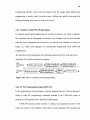
2.4.3 Computer-Assisted Part Programming
.
In computer-assisted part programming, the machine instructions are written in English,
like statements that are subsequently translated by the computer into low-level machine
code that can be interpreted and executed by the machine tool controller. As shown in
Figure 2.2, widely used languages are Automatically Programmed Tools (APT) and
COMPACT II.
The main tasks of the programmer are to defining the geometry of the work part and to
specifying the tool path and operation sequence.
Figure 2.20 Tasks in computer assisted programming.
2.4.4 NC Part Programming Using CAD/CAM
In this programming, the part program is directly prepared from the CAD part geometry,
either by using NC programming commands included in the CAD/CAM system or
passing the CAD geometry into a dedicated CAM program.
CAD/CAM systems provide facilities to display the programmed motion of the
cutter with respect to the workpiece, which allows visual verification of the program and
35
the ability to edit interactively a tool path with the addition of tool moves, standard
cycles, and perhaps APT macros ( or the equivalent from other languages).
2.5 Data Preparation for Numerical Control
A post-processor is used to convert the machine-independent code format into a format
suitable for the machine tool (machine control data, MCD). The machine receives
instructions as a sequence of blocks containing commands to set machine operations,
parameters, dimensional, and speed data. The classification of identifiers for the
commands is as follows:
1- N. Sequence number: Is simply the identifying number for the block, in ascending
numerical order, but not necessary in a continuous sequence.
2- G. Preparatory functions: Prepare the MCU for a given operation, typically
involving a cutter motion.
3- X, Y, Z, A, or B Dimensional Data: Contain the location and axis orientation data
for a cutter move.
4- F — Feed functions: Are used to specify the cutter federates to be applied.
5- S — Speed functions: Are used to specify the spindle speed, or to setup parameters
for constant surface speed operation.
6- T — Tool functions: Are used to specify the cutter to be used, where there are
multiple choices, and also specify the particular cutter offset.
36
7- M — Miscellaneous functions: Are used to designate a particular mode of
operation, typically to switch a machine function ( such as coolant supply or
spindle) on or off.
2.6 Case Study for NJIT FMS
Chamfering program
Chamfering operation takes place by chamfering 7" X 7" Plexiglas block in 45 ° as shown
in Figure 2.22. Olivetti machining center through CNC instructions shown in table 2.2
does chamfering operation.
Table 2.2 Suggested Program for Olivetti Machining Center " Chamfering Operation"
Sequence
number
Preparatory
functions
X
Y
N001
G54
0.000
0.000
N002
.0.500
N003
S
...
M
03
.7.00
N004
.7.00
N005
+7.00
N006
N007
N008
N009
Z
+7.00
G54
+3.00
0.000
0.000
0.000
05
Program End
Figure 2.22 Dimensions of the chamfered block.
Notes
Rapid travel to start point
Adjust Z height and start
cutting
Start cutting and move in
negative X direction
Continue cut and move in
negative Y direction
Continue cut and move in
Positive X direction
Continue cut and move in
negative Y direction
Move away from Piece
Rapid travel back to start
Turn off motor
37
Drilling and milling program
Drilling and milling operations performed as drilling four holes, a hole in each corner.
The milling operation performs fabricating NJIT FMS on the top surface of the work
piece. Appendix C has the CNC program instructions to perform both operations. In
milling operation or any similar operation, there are special motions for the cutting tool
path; such as circular motions, these special motions have been formulated in
mathematical formulas to facilitate their CNC programming. Examples for useful
formulas are shown in Appendix B.
CHAPTER 3
INDUSTRIAL ROBOTS AND INTERFACE WITH CAD SYSTEM
3.1 Introduction
Robotics is a wide field currently sought after for research and development. There are
many robot software available today. New software are released periodically, they
become increasingly user-friendlier, compatible with working the environment, and
possess more powerful features to control the robot. However, these software are
designed to control one specific robot or a unique family of robots. Recently, software
have been developed that are compatible with the robots of any manufacturer. The price
of the package is affected by the complexity of its programming. For example, there are
packages that cost $25000 or more, like the PLACE graphic simulator.
The software used one in this chapter is Workspace ™
3 and works in the DOS
environment. There are new versions of this software, such as Workspace ™ 5, which
works in Windows.
Workspace ™3 is an off-line programming, graphical robot simulator that offers
accuracy and compatibility regardless of what major manufacturers robot is used. The
benefit of Workspace ™3 is that it helps to visualize of the robot process quickly before it
goes into the production stage.
38
39
3.2 Programming Techniques
Robots are programmed using manual setups leadthrough programming, computer like
robot programming languages, and off-line programming. Manual setup techniques are
usually associated with limited sequence robots where limit switches and mechanical
stops provide robot control.
Leadthrough programming involves teaching a particular task by moving the
robot's manipulator through a sequence of motions and recording the position
coordinates. Computer like robot languages involve a specific set of instructions that
provide robot control, from a simulated CAD model, Off-line programming is
accomplished by sending a set of instructions to the robot controller. This minimizes the
time a robot must be taken out of production in order to accomplish the programming.
A PC based CAD system interfaced with an industrial robot is beneficial over the
standard robot programming techniques since robot programs can be generated
automatically by a set of graphical instructions displayed on the computer screen. Once
proper kinematics and geometries are established, a graphical simulation of the
workcell's function will occur in real-time, allowing for modification and improvement
before generated programs are downloaded into the robot's controller.
3.3 Robot Software
A robotic McDonald Douglas CAD software system consists of four modules, namely
PLACE, BUILD, COMMAND, and ADJUST. The relationship among these modules is
shown in Figure 3.1.
Figure 3.1 Process flow from simulation to translation.
The PLACE (Positioner Layout And Cell Evaluator) module is used to develop a model
of the workcell similar to the actual working system. It is also useful in simulating all the
operations of the FMS cell on the system so that the various layouts and motion
sequences can be animated and evaluated.
The BUILD module enables the user to graphically build any additional robots or
other devices that are not in the CAD data base. These geometric models of the new
robots and devices can be automatically combined with their unique kinematics
description for future animation in PLACE.
41
The COMMAND module is used for programming the robots off-line.
COMMAND is used in conjunction with PLACE and a specific robot program translator
to generate a complete robot program that can be downloaded to and executed on the
robot controller. A powerful feature of COMMAND permits the user to associate groups
of logic instructions with specific robot positions defined by a place sequence.
The ADJUST module is used in conjunction with a probe attached to the robot
end effector. It is designed to modify the locations of the robot end effector in a PLACE
workcell so that the physical dimensions of the robot match the actual locations of the
corresponding end effector in the actual FMS cell. This is a fast and efficient way of
resolving any discrepancies that may exist between the physical dimensions of the actual
robot and the dimensions of the simulated model and also between the actual cell and its
computer model.
3.4 Robot Anatomy
All robots have joints and links. The anatomy of robot is a description of its joints and
links.
IBM 7535 Robot
The IBM 7535 robot was shown in Figure 1.9 has special end effectors to perform
drilling operation. The robot has SCARA configuration. The arm is very rigid in the
vertical direction allowing the robot to perform drilling operation by moving the drill
only up and down in vertical direction. This robot consists of number joint and links. It
has five degrees of freedom with three types of joints; orthogonal, rotational, and
revolving. In orthogonal joint. The relative movement between the input link and the
42
output link is a linear sliding motion. The input and the output links are perpendicular to
each other. It is called 0 joint and is shown in Figure 3.2a. Rotational joint provides a
rotational relative motion of the joints with the axis of rotation perpendicular to the axis
of the input and output links. It is called
R joint and is shown in Figure 3.2b. In revolving
joint. The axis of the input link is parallel to the axis of rotation of the joint, and the axis
of the output link is perpendicular to the axis of rotation. It is called V join, and shown in
Figure 3.2c.
Figure 3.2c Revolving joint.
GE P-50 Robot
The GE P-50 robot was shown in Figure 1.10 has a vacuum gripper to enable picking up/
depositing a block from/to the cart. It has a jointed arm configuration, with the arm being
able to swivel about the base. This robot consists of rotational joints and twisting joints.
The rotational joint allows for a rotational motion of the links with the axis of rotation
perpendicular to the axis of the input and output links. It is called
R joint, and is shown
43
in Figure 3.3a. The twisting joint permits a rotary motion, but the axis of rotation is
parallel to the axis of the two links. It is called T joint and is shown in Figure 3.3b.
Figure 3.3a Rotational joint.
Figure 3.3b Twisting joint.
GMF Ml Robot
GMF M1 robot was shown in Figure 1.11 has a mechanical gripper, and a cylindrical
configuration, It consists of a vertical column, relative to which an arm assembly can be
moved up and down. This robot consists of an orthogonal joint, twisting joint, and linear
joint. The orthogonal and twisting joints were discussed earlier. In linear joint the relative
movement between the input link and the output link is a linear sliding motion, with the
axes of the two links being parallel. it is called L joint. And shown in Figure 3.4.
Figure 3.4 Linear joint
44
3.5 WorkSpace™3 Robot CAD System
With the assistance of modern computer technology, design, simulation, control,
planning, management, or any area of manufacturing is no longer difficult to model. It
has been said that "3D simulation has revolutionized the way that engineers can
work".[6]. The following sections describe how the computer simulation done by
Workspace™
3 was used to simulate the drilling operation done by the IBM 7535 robot.
Workspace ™3 is widely used in industry tool to design, model and simulate. It
can be used in off-line programming, which means that it can prepare the program and
download it to the robot without interrupting production. The features, specifications and
applications of Workspace ™3 are discussed below.
3.5.1 Features
Workspace™3 is a 3D graphical simulation software system for robotics and
mechanisms. It is a productive tool designed to make the implementation of advanced
manufacturing systems as simple and economical as possible. Workspace™ increases
productivity and reduces time [34]. The features are:
1. Quickly model work cell layout
2. Demonstrate process and plant design
3. Prepare real time animation for presentation
4. 3D CAD system constructive solid geometry
45
3.5.2 Specifications
1. Teach point files
2. Graphical representation results
1. Ability to easily off-line programming
2. Kinematics modeler
3.5.3 Applications
1. Arc and spot-welding
2. Materials handling
3. Paint spray
4. Palletizing
3. Electronics assembly
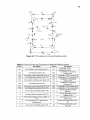
Table 3.1 is an example of controlling the robot motion using Workspace ™3 . It describes
the joints and points positions for the SCARA industrial robot for a drilling operation.
Initially after the robot is built, the joints have home position values in the X, Y and Z
axes as: X: 708", Y: 2", and Z: 204", and the values of rotational axes a, b, and c around
each axis are a:0° b:0° and c:0°, if the joint is taught to move the point 1 then the
coordinates will be changed and the new points called TP1, its values are shown in the
table below. So there are four teach points to perform drilling operation done by the IBM
7535 robot
46
Table 3.1 Coordinates of the Points with Joints Motions of IBM 7535Robot
Points
HOME
Joints
1_ 0_
2
0
3
0
4
0
X
708
Y
2
Z
204
a
0
b
0
0
c
TP1 I TP2
TP3
TP4
0
45
0
0
618
223
204
0
0
0
0
45
45
75
618
221
129
0
0
90
0
45
45
0
618
221
204
0
0
90
0
45
45
0
618
221
204
0
0
90
3.6 Case Study: Sample Program for Drilling Operation done by NJIT FMS
The program presented here shows how WorkSpace ™3
can be used to program the IBM
7535. It also shows the parameters, which should be considered in the programming. To
understand this program, the following definitions are needed:
•
Karel 2. The language for the simulation and for writing this program.
•
Teachpoint (TP). The point, where the joint should rest by the end of the
movement.
•
Position. The defined position for each teachpoint.
•
NullObject. Hidden object used to join two objects.
•
AttachObject. A command likes the same but to attach the block to the cart.
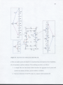
Referring to the Figure 3.5. If the yellow bar rotates about the X-axis by 4) degrees,
the transformation matrix for that rotation is Rot (X, 4) ). Similarly, if the rotation
47
takes a place around Y-axis or Z-axis, the rotation matrices are Rot (Y, I) and Rot (Z,
CD) respectively. These matrices are shown below.
Figure 3.5 Rotational axes around X-axis by angle (I)
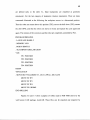
The program below traces the robot from an ISOMETRIC view. It consists of
three types of statements; auxiliary statements, geometry statements, and motion
statements.
The first five statements in the program are the auxiliary statements. The program
begins with the declaration of the program name, which is DRILING. Then it declares the
language (Karel2), the memory is 1024kb, the name of the robot IBM 7535, and then it
moves to teachpoint declaration, {then there are four teaching points and their positions
48
are defined early in the table 3.1, these teachpoints are classified as geometry
statements). For the last category of statements (motion statements). There are many
commands illustrated as the following, the workpiece moves to a determined position.
Then the robot arm comes above this position (TP2), moves the drill down (TP3), rotates
the drill (TP4), and then the robot arm moves to home and repeats the cycle again and
again. The motions of the conveyors and the robot are completely controlled by PLC.
PROGRAM DRILLING
. LANGUAGE KAREL 2
. MEMORY 1024
. ROBOT IBM7535
. TEACHPOINT DECLARATION
VAR
TP1: POSITION
TP2: POSITION
TP3: POSITION
TP4: POSITION
BEGIN
%INCLUDE 2#
. MOVE OBJ `NULLOBJECT1', 201.31,709.62, .208.31,250
MOVE TO TP2
MOVE TO TP3
MOVE TO TP4
MOVE TO $ HOME
END DRILLING
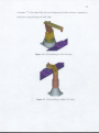
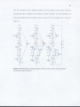
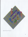
Figures 3.6 and 3.7 show examples of robots used in NJIT FMS drawn by the
well known CAD package AutoCAD. These files can be exported and imported by
49
Workspace ™3 . The whole FMS cell can be displayed by CAD as shown in Appendix A,
which shows many drawings for NJIT FMS.
Figure 3.6 CAD modeling for GE P-50 robot.
Figure 3.7 CAD modeling for IBM 7535 robot.
CHAPTER 4
COMPUTER VISION INSPECTION
4.1 Introduction
Over the past twenty years, computer vision has been used in wide array of
manufacturing applications, including robotics, electronics and semi conductor
manufacturing. These were among the first to embrace the technology and currently
account for about half of the computer vision applications found on factory floors.
However acceptance is rapidly growing throughout the entire manufacturing
sector, with computer vision systems now in place in food processing, pharmaceuticals,
wood and paper, plastics, metal fabrication and other industries. Until recently, the
limiting factor in vision-based robotic control has been the ability to perceive and react in
complex and unpredictable surroundings.
Computer Vision and Image Understanding is a prestigious journal devoted to the
dissemination of research in areas relevant to computer vision. Papers are published on
all aspects of image analysis, from low-level processing, as in early vision, to high-level
symbolic processing needed for recognition and interpretation. More specifically, the
following topics are particularly central to what is published in the journal:
•
Computational models of the human visual system
•
Early vision
•
Data structures and representations needed for high-level vision
•
Shape representation and extraction
50
51
•
Range data analysis
•
Use of motion for recognition and interpretation
•
Matching and recognition
•
Architectures and languages for image processing
•
Vision systems
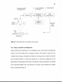
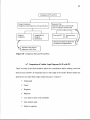
4.2 Operations of Computer Vision
Computer vision inspection can be defined as a method of using a computer to analyze an
image obtained from a video camera. The operation of the vision system can be divided
into the following three functions: [27]
1- Image acquisition and digitization
2- Image processing and analysis
3- Interpretation
These functions and their relations are illustrated schematically in Figure 4.1.
52
Figure 4.1 Basic functions of a machine vision system.
4.2.1 Image Acquisition and Digitization
Image acquisition and digitization is accomplished using a video camera and digitizing
system to store the image data for subsequent analysis. The camera is focused on the
workpart and an image is obtained by dividing the viewing area into a matrix of discrete
picture elements (Pixels), in which each element has a value that is proportional to the
light intensity of that portion of the scene. The intensity value for each pixel is converted
into its equivalent digital value. The operation of viewing a scene consisting of a simple
object is depicted in Figure 4.2.
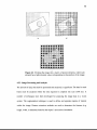
Figure 4.2 Dividing the image into a matrix of picture elements, where each
element has a light intensity value corresponding to that portion of the image.
4.2.2 Image Processing and Analysis
The amount of data, that must be processed and analyzed, is significant. The data for each
frame must be analyzed within the time required to complete one scan (1/30 sec). A
number of techniques have been developed for analyzing the image data in a vision
system. The segmentation technique is used to define and separate regions of interest
within the image. Feature extraction methods are used to determine the features (e.g.
length, width, or diameter) based on the object's area and its boundaries.
54
There are two commonly used segmentation techniques. The threshold technique,
which involves the conversion of each pixel intensity level into a binary value. This is
done by comparing the intensity value of each pixel with a defined threshold value. If the
pixel value is greater than the threshold, it is given the binary value of white (e.g. 1). If
the value is less than the defined threshold, it is given the bit value of black (e.g.0).
Another segmentation technique is edge detection. It determines the location of
boundaries between an object and its surroundings in an image. This is accomplished by
identifying the contrast in light intensity that exists between adjacent pixels at the borders
of the object.
4.2.3 Interpretation
The interpretation function is usually concerned with recognizing the object, a task
termed object recognition or pattern recognition. The objective of this task is to identify
the object in the image by comparing it to predefined models or standard values. Two
commonly used techniques are template matching and feature weighting. The most basic
template matching technique is one in which the image is compared, pixel-by-pixel, with
a corresponding computer model. Within certain statistical tolerance, the computer
determines whether or not the image matches the template. Several examples of this are
shown in Figure 4.3.
55
Figure 4.3 Diverse applications for which machine vision has been implemented.
The process begins with an image that is formed from a camera lens using a camera
receiver. The receiver is a CCD (charged coupled device) array, which converts the
image into a grid of separate points, called pixels. The pixels are seen as squares on the
grid. Each pixel is light sensitive and therefore has an electronic charge, which is
representative of the amount of light, the lens projects onto them.
The electronic signals are sent to a processor where an analog to digital converter
coverts the signals into a series of binary numbers and stores them into memory. Each
pixel is therefore assigned a numerical value that represents a particular intensity of light.
The light intensity number corresponds to a grayscale indicator that uses values from 0 to
63 (0 begin black and 63 begin white).
Intelligent Visual Sensor (IVS) systems can analyze the converted image in a
number of ways. IVS use algorithms that can identify measurements, edge detection, part
defects, and other parameters. These algorithms can be used simultaneously to detect
56
acceptable and rejectable parts. During an inspection, the system could use a triggering
device, such as a photoelectric sensor, to enable the camera to acquire an image of the
object that is being inspected. The image would then be converted to a digital array and
stored into a buffer. The vision system could apply an algorithm such as counting edge
pixels and comparing them to a standard value for this measurement. The values
generated can be used to calculate other functions within the IVS system before sending
an output through RS232 communications to an external device such as a programmable
logic controller.
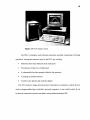
4.3 The Itran IVS Computer Vision System
The IVS system used for the project is a feature sensor system. The feature sensor
contains area tools, which can be configured in different ways. There are quite a few
components of the system, which need to be configured for the application. The software
used to configure and edit the system is the SensorEdit software supplied by Itran. The
software is used on a PC, which contains a link card and cable used to communicate with
the IVS.[14]
The pixel resolution for Itran IVS system is 320 x 240 pixels. The IVS system has
sub-pixel resolution capabilities to 1/32 of a pixel. This is done by using mathematical
operations of differentiation and interpolation on the surrounding pixel values. Because
of this technology, the accuracy of the system is greatly increased.
The total processing time of the IVS system is constant of each inspected part at
67 msec. Time is needed for scanning (at fixed rate) and the implementation of a parallel
57
processing technique. The system is actually processing four images at one time. There
are four steps for each inspection, and each of the four images that are being processed
advance to the next step. The four steps are as follows:
1) Read inputs, acquire image, apply locator and lightmeter.
1) Apply the vision algorithms.
2) Process the worksheet calculations.
3) Process outputs.
4.3.1 Obtaining an Image
The first step in obtaining an image is to place a part in the inspection area and within the
field of view. Using the software, the system is configured for continuous inspection in
order to obtain a live video image on a display monitor. Lighting and focus adjustments
are made until the image is optimized. Next, using the Itran software, a converted digital
image of the object is obtained. A magnifier tool, which enables one to see the values of
the pixels within the image, can be used to determine if any additional lighting or
focusing issues need to be addressed to obtain a clear contrasted image. The magnifier
also helps determine the threshold settings that need to be used for the inspection.
4.3.2 Area Tools
The area tool is a technique used to measure certain selected functions within a selected
(or highlighted) area within the field of view. The functions include sum edge energy,
count edge pixels, sum gray values, and count threshold pixels. For this application, the
count threshold pixels function was used which provides the total number of pixels
58
values above or below a specified threshold value within the area tool. The threshold
value must also be determined. The IVS software provides a histogram of the pixel
values within the area tool, which is used as a. guide in determining the optimum
threshold value. The count threshold function was set to count the number of pixels that
had a value above the threshold value of 9.
The area tool was inserted and placed over the image of the largest part in order
for it to be large enough for all six different parts. After the application was downloaded
to the IVS, each part was manually placed in the inspection area to measure the area tool
value for that part. Once all the values were obtained, the output of the system was
configured. This procedure is used after uploading an image (a new image from the
camera), and positioned the locator tool; these tools are listed as following:
1. Select Edit Arc Tools.
2. Select a Brush Shape.
3. "Paint" an Area Tool.
4. Select Inspection Method.
5. Repeat For Additional Tools.
4. Resolve Tool Conflicts.
5. Program the 110.
6. Program the Math Worksheet.
7. Download and Test the Application.
59
4.3.3 Screen Messages, RS232 Outputs and Discrete I/O
The IVS system allows one to create outputs in three different forms: discrete I/O, screen
messages, and RS232. The output can be configured using Boolean logic or can be set to
true or false. The discrete I/O is opto isolated hardwired outputs, which can be wired to
any external device. The screen massages are displayed on the vision system display
monitor. The RS232 output information can be sent to a wide variety of RS232 terminals
including PC's and PLC's.
Screen messages and discrete I/O are created using Boolean logical formulas. A
sample formula could be: IF (AREA 1>24000 AND AREA 1<26000,TRUE, FALSE).
Here 24000 is the least number of threshold pixels and 26000 is the maximum number of
threshold pixels. The AREA 1 is the name of the area tool, TRUE is the 'then' statement
and the FALSE is the 'else' statement. The message display is then configured to
determine what was to be displayed. Each part is then assigned an output port, which is
used as hardware interface to the PLC.
RS232 outputs are configured exactly the same way as the screen messages and
discrete I/O. The only difference is that the RS232 outputs setup needs to be configured
in order to send the data in the proper format for the receiving device. Items such as baud
rate, data bits, stop bits, and terminators are configured.
4.4 The FS11 — Feature Sensor
The FS 11 is an innovative, low cost, non-contact, feature sensor. It is capable of highspeed operation, performing multiple feature inspections per part. As shown in Figure
4.5.
60
Figure 4.4 FS 11-feature sensor.
The FS 11 is primarily used following automatic assembly, machining or forming
operations. Among the numerous uses for the FS 11 are verifying:
•
That holes have been drilled in sheet metal parts
•
The absence of flash on a modeled part
•
A subassembly has been properly added to the operation
•
A package is properly formed
•
A bottle cap is present and correctly shaped
The FS 11 delivers image derived process information to production control devices
such as programmable logic controllers, personal computers, or any control system. It can
be directly connected to process machinery using standard industrial I/O.
61
On-line operation
The FS 11 grabs from a video camera a 2D image of the part to be inspected. The image is
processed in 16.7 milliseconds using Iran's proven and sophisticated gray scale
technology. Up to 128 feature inspections can be made on each image.
A powerful comprehensive set of math operations combines and manipulates the
inspection results, allowing that implement real time solutions. It can be used to perform
inspection and other tasks associated with manufacturing processes. A built-in shift
register tracks parts and permits effective reject control, even on high-speed processes
(up to 60 parts/sec).
Simplified System Integration
The FS 11 has been designed to simplify its integration into a manufacturing line. Its
features include:
Built-in material handling shift register for effective rejection control, even on
•
high-speed processes
•
Integrated sensor and strobe circuitry (for those systems requiring strobes)
•
Built-in user menu for system setup, including options to control monitor display
and camera setup
Benefits/Features
•
•
Fast
-
All measurements made in 16.7 msec
-
Pipelined processing allows rates up to 60 parts per second
Non-contact
-
2D visual analysis of parts
62
•
•
•
Easy to Use
-
Graphic setup environment on MS Windows 95 or more
-
Speed and response rate are unaffected by the complexity of inspection
-
Automatic compensation for object motion and lighting variation
Communications
-
RS 232
-
Discrete I/O
-
Built-in shift register for interfacing with material handling system
Flexible
-
•
•
Measurements can be made along any line or contour
Visual feed back provided for operators
-
RGB/monochrome RS 170 monitor output
-
Real time display of images and vision tool graphics
-
Screen message reports results
Meet special application needs
-
Sensor development kit allows tailoring the sensor to meet specific
application demands
4.5 Inspection Method
In the SensorEdit program, there is a Method menu, which contains the methods used to
control the computer vision system regarding the acceptance or rejection the inspected
part. Several options are available on the this menu as indicated below:
63
1. Sum gray values. Sum the gray scale values of all pixels in the tool. Suppose there are
four pixels in the tool having gray scale values of 20, 23, 24, and 26. This function
returns a value of 93.
2. Count threshold pixels. Counts all pixels with gray scale intensity values equal to or
above the threshold that has been set.
3. Count pixels below threshold. Counts all pixels with gray scale intensity values below
the threshold that has been set.
4. Sum edge energy. Sums the edge strength values of all pixels in the tool.
5. Count edge pixels. Counts the pixels with edge strength values equal to or above the
threshold.
The focus will be "Count threshold pixels", "Counts pixels below threshold" and
"Count edge pixels". Changes can be done to the threshold values by selecting image
brush thresholds Figure 4.5, a dialog box displays a histogram of the image, in this box,
lower and upper thresholds can be updated to show the qualifying pixels.
The histogram is a vertical bar chart set on a horizontal axis of 63 gray-scale
values. The height of each bar shows the relative number of pixels at each gray-scale.
Value. For example, if the bar over the gray-scale value 33 is twice as high as the bar
over the gray-scale value 32, then there are twice as many pixels in the region with grayscale value of 33 as there are with a value of 32.
64
Figure 4.5 Tooth brush threshold.
4.6 Project Description
The IVS system was configured to identify "NJIT FMS", which is fabricated on the
NASA II CNC milling machine and shown in Figure 4.6. The IVS system scans the part
as it passed the lens and matches its image with qualifying logical expressions that were
created for each part. Screen messages were displayed for the identification of each block
accordingly.
Using the RS232 input of the IVS system, a terminal software program using
windows software was used to display and store the inspection data for each "NJIT FMS"
work part, make comparison with a predefined image and energize the robot to place
each part the accepted or rejected bins
Figure 4.6 model of the inspected workpart.
CHAPTER 5
PROGRAMMABLE LOGIC CONTROLLERS
5.1 Introduction
Today manufacturing becomes increasingly flexible and fully automated to achieve faster
and better quality production, and to stay on the competitive edge. Programmable logic
controllers (PLCs) are used in most industrial applications control. They are considered
as an integral and invaluable tool that helps designers and decision makers to better
implement their long term manufacturing control plans by using computer hardware and
software.
A PLC can be defined as a digitally operating electronic system designed for use
in an industrial environment to implement specific functions such as sequencing, timing,
counting and arithmetic control function and analog functions such as proportionalintegral-derivative (PD). Ladder logic diagram LLD is used to program PLCs.
A Ladder Logic Diagram is a graphical programming language consists of a set of
rungs each of which instructs the PLC to scan input(s) and activate output(s). A rung is
bounded by two vertical lines representing the negative polarity on the left and positive
polarity on the right. Each rung describes the current flow from component(s) on the left
side of the rung (input(s)) to the right side component(s) of the rung (output(s)).
A PLC study is presented in this chapter. Components of PLCs in Section 5.2,
functions and advantages of PLCs in Sections 5.3 and
65
66
5.4 respectively, and the basic logical gates of PLCs in Section 5.5. The case study for the
PLC used in NJIT FMS is presented in Section 5.6.
5.2 PLC Devices
State-of-the art PLC devices are used as controllers in assembly lines, robots and other
manufacturing facilities that facilitate precise control measurements. Those devices can
be digital or analog and used as inputs to the system or outputs from the system.
Examples of devices used with PLC are listed in table 5.1 and examples for the input
devices used in NJIT FMS are shown in Figure 5.1
Table 5.1 Input and Output PLC Devices
Input Devices
Limit switch
Photo detector
Pushbutton switch
Control relay
Circuit breaker
Timer
Output Devices
Motor
Alarm buzzer
Control relay
Lights
Valves
Solenoid
Figure 5.1 Examples for input and out devices; (a) Limit Switch, (b) Photo detector,
(c) Solenoid.
67
5.3 PLC Components
A PLC has the following components:
I. Input module
2. Output Module
3. Processor
4. Memory
5. Power Supply
6. Programmable Device
The components of a PLC controller and their functions are shown in Figure 5.2.
Figure 5.2 Schematic diagram of a PLC controller.
68
5.4 PLC Computer Functions
The functions that a PLC can perform are:
1. Control of each process station
2. Production control
3. Traffic control
4. Tool control
5.5 Advantages of PLC
PLC use offers the following advantages:
1. Increase system availability
2. Decrease downtime requirements to recover from failure
3. Decrease cost from material and man-hours for installation
4. Increase system feasibility.
5. Increase flexibility to meet new requirements
5.6 Basic Logic Gates used in PLC (AND, OR, and NOT)
A logical AND gate outputs a value of 1, if all inputs are 1. A logical OR gate outputs a
value of 0, if all inputs are 0. Logical NOT gate output is 1 if the input is 0, and vice
versa.
Table 5.3 shows the three basic logic gates with their presentations as Logic gate,
electrical circuits and LLD presentation.
69
Table 5.3 Basic Logic Gates Used in PLC
For better visualization of how the programming language LLD is designed, see the
example shown in Figure 5.4. In the first rung, pressing input switch I:1/1 activates the
output 0:6/1, which can be any output device. The next rung describes a logic AND gate.
To energize output 0: 6/2 both input switches or devices should be energized. The third
rung describes a logic OR gate. Output 0:6/6 can be activated if either one of inputs 1:2/4
or 1:6/12 or both should be pressed.
The following rung describes the latching concept in PLC programming. Once the
switch 1:2/4 is pressed or activated, the circuit is closed and output 0:5/1 is energized. It
will remain on, irrespective of whether the previous switch is off or on. The function of
switch I:1/2 is to let the current flow through the circuit for the first time and to cut off
the circuit whenever is needed, it might be used as emergency switch.
70
The fifth rung shows a timer element. When switch I: 2/2 is pressed the output
goes on and the timer starts timing for four seconds. When the timing is over, output 0:
6.12 goes off and the timer sends a signal to the following rung to activate output 0: 6/4
Figure 5.4 An example for LLD programming
The seventh rung shows counter element. Here after the switch I: 1/3 senses something 5
times, the counter sends a signal to the following rung to activate it and output 0: 6/7
71
goes on. To reset the counter, a different input switch should be used. as shown in the last
rung.
5.7 Case Study of NJIT FMS
Operational Descriptions
The working cycle for this FMS proceeds in the following five states:
State 1: Loading Carts State.
1. Initially all four carts on the conveyor system are empty and available for the raw
materials to be loaded onto them from the parts presentation station.
2. The GE robot P-50 goes to the parts presentation station and loads four parts, one by
one, onto the four carts on the conveyor system. The carts move clockwise as they are
being loaded.
3. Once the four parts are loaded, the positions acquired by the four carts are shown in
Figure 5.3
Figure 5.3 Loading state of the conveyor system.
72
State 2: Drilling Operation.
The 113M7535 robot drills four holes on each of the corners of each blank part as the cart
stops at the drilling machine.
State 3: Chamfering Operation.
1. The GMF Ml robot moves to position x6 of cart C and picks up the part from the cart
and places it into the fixture of the Olivetti machining center.
2. Once the part is loaded on the chamfering machine, the robot retracts, and the
chamfering machine chamfers the edges of the upper surface as required.
3. After the chamfering machine operation, the robot moves to the Olivetti machining
center to remove the part that was machined from the holding fixture back to cart C.
State 4: Milling Operation.
1. The GE P-50 robot moves to the conveyor to remove the part from the cart position X1
and loads it into the fixture located on the CNC machine table.
2. Once the part is loaded on the CNC milling machine, the robot retracts, and the milling
machine mills the rectangular part as required.
3. After the milling machine operation, the robot moves to the milling machine to remove
the part that was machined from the holding fixture.
4. The robot returns the finished part to the same cart on the conveyor.
State 5: Vision Inspection
1. A signal is sent to the vision camera to inspect the part.
2. The vision system analyzes the part and outputs a signal that directs the PLC to tell the
robot to accept or reject the part.
73
3. The robot runs either an accept program to place the part in the accept bin or runs a
reject program to place the part in the reject bin.
The entire operation with its control points is shown in Figure 5.5. For more
information about the PLC — LLD used to control NJIT FMS cell refer to appendices E,
F, and G
Figure 5.5 Control points of NJIT FMS operation.
CHAPTER 6
PETRI NET MODELING AND SIMULATION
6.1 Introduction
the use of technology and the application of control and management theories and
techniques have revolutionized the flexibility of manufacturing. New control and
modeling techniques are always sought for the purpose of achieving further
improvements. A technique that has the potential for generating additional improvements
is the use of Petri nets.
The focus of this chapter is primarily on Petri nets (PN) and their contribution to
industry development. Definitions are discussed in section 6.2; classifications of PN in
section 6.3; modeling methods in section 6.4; a case study of NJIT FMS in section 6.5;
and finally the connection between Petri Nets and PLC in the last two sections.
74
75
6.2 Petri Net Definitions
Petri Net: A Petri net is a graphical and mathematical modeling tool, which is able to
model concurrent, asynchronous, distributed, and parallel systems. The basic Petri net
consists of four different components: Places, Transitions, Arcs, and Tokens.
Place: A Place is a basic Petri net component, which represents a condition and
represented by a circle. If a place is a member of the input function of a transition, it is a
precondition for that transition or event to occur. If a place is a member of the output
function of a transition, it is a post-condition of that transition.
Transition: A transition is a basic Petri net component, which represents an event. The
event may occur when all of the input places to the transition contain enough tokens to
enable the input arcs to the transition. The occurrence of the event, also known as a
firing of the transition, will result in tokens being deposited through each of the output
arcs of the transition into the respective output places.
Arc: An arc is a Petri net component, which relates places to transitions and transitions to
places, and has an associated weight, representing the number of tokens needed to enable
the arc.
Token: A token is a basic Petri net component, which is thought of as residing in a
`place'. A token signifies that a particular place, or condition, is true. Multiple tokens
residing in a place are usually representative of the existence of multiple resources.
Reachability Tree: A reachability tree represents all of the obtainable markings for a
Petri net. The tree begins with the initial marking, with a line from the initial marking to
a new marking for each enabled transition.
Marking: A mapping of tokens to places, which defines a state for the Petri net.
76
Live: A Petri net is live when there exist no terminal nodes in the net's reachability tree.
For each marking in the reachability tree, there exists at least one transition that is
enabled for that marking.
Safe: A place is said to be safe if, for all possible markings, the number of tokens in that
place never exceeds one. The Petri net is declared safe if all of the places in the net are
safe.
Bounded: A place is k-bounded when, for each marking in a reachability tree, the
maximum number of tokens appearing in that place never exceeds k. A Petri net is jbounded if all places in the net are bounded and j represents the maximum bound value of
all places in the net. k represents maximum number of tokens in specific place.
Conservative: A Petri net is said to be strictly conservative if, for all possible markings,
the total number of tokens in the Petri net always remains constant. A Petri net may also
be conservative with respect to a weighting vector such that all markings when multiplied
by the weighting vector are equal. [31&35]
6.3 Petri Nets
Petri net models can be either mathematical or applications
6.3.1 Mathematical Models
A Petri net is four-pillars:
PN= [P, T, I, 0]
P: a finite set of places I P.
• • • ,PE,
77
T: a finite set of transitions, ft t
t
I: an input function, (TxP) 4 {1,0}
0: an output function, (TxP) 4 {0,1}
Mo : an initial marking P4 N where N = {0,1,2,...}
< P, T, I, 0, M o> a marked Petri net.
To start analyzing the PN, assume the process shown in Figure 6.1.
Figure 6.1 An example of processing which analyzes the
mathematical modeling of a PN.
Where
P = {P1, P2, P3, P4}
Mo = (1,0,1,0)
Enabling Rule A transition is enabled if every input place contains at least one token.
78
Firing Rule The firing of an enabled transition occurs by removing one token from each
input place of the transition, and adding one token to each output place of the transition.
The enabling and firing rules are illustrated in Figure 6.2
The above rules can be explained in detail using the Petri net example shown in
Figure 6.1. It consists of four places and three transitions, initially M. = (1,0,1,0), so for
ti to be enabled it should have two tokens; one from P1 and another from P3. Both
tokens are available in this example, so the firing takes a place and the token moves to
P2, meaning that processing is activated. Transition t2 has one input and two outputs, so
once the token is in P2, automatically t2 has been enabled, and the token moves to places
P3, and P4. In this state t1 is not enabled because it doesn't have a token in P1 while t3 is
enabled. So P4 fires the token to P1 and process recycles it self.. Figure 6.2 shows every
enabled transition and their firing places. Table 6.1 describes the reachability tree for this
Petri net
Figure 6.2 Transition of tokens, which is based on enabling and firing rules.
79
Table 6.1 Reachability Tree for Figure 6.2
State before
(1,0,1,0)
(0,1,0,0)
(0,0,1,1)
Transition
.T 1 .>
.T2.>
.T3.>
State after
(0,1 ,0,0)
(0,0,1,1)
(1,0,1,0)
6.3.2 Applications
➢ Petri nets can be used in the following applications:
Manufacturing, production, and scheduling systems
➢ For sequence control, both modeling and visualization and generating the code for
a (PLC)
➢ Communication protocols and networks
➢ An alternative to finite state machines and state diagrams
6.4 Modeling Methods
The basic relationships between processes in any automated manufacturing line and their
representation by PN can be classified as shown in Table 6.2, which shows the modeling
method, definition of that method.
80
Table 6.2 Manufacturing Processes and Their Annlications by PN
One of the major advantages of Petri nets is their ability to analyze a system for
properties related to manufacturing control. These properties include boundedness or
safeness, liveness, and reversibility. Their significance to manufacturing systems is as
follows:
1- Boudedness or safeness implies the absence of capacity overflows, which assures
there is no overflow. Safeness is a special case of 1-boundedness
2- Safeness of a resource place indicates the availability of only a single resource
3- Liveness implies the absence of deadlock; this property guarantees that a system
can successfully produce tokens
81
4- Reversibility implies the cyclic behavior of a system; it means the system can be
initialized from any reachable state
For Petri net, there are conditions that have to be furnished to understand the analysis of
modeling and analysis of reachability tree. The latter is considered to be an important tool
for the following conditions:
1- If all the places have one token at any firing stage, which means the system is 1.
Bounded and safe.
2- If the system continues to produce tokens, that means the system is live.
3- If from any reachable state the system can be initialized, that means the system is
reversible.
6.5 Case Study: Modeling and Analysis of PN for NJIT FMS
6.5.1 Description and Modeling
The material handling system of NJIT FMS cell was modeled using Petri net. The
modeling is shown in Figure 6.3 and the description of its places and transitions is shown
in table 6.3. Table 6.4 shows the reachability tree for material handling system
82
Figure 6.3 PN modeling for a material handling system.
Table 6.3 Places (Events) and Transitions for Material Handling System
Event
Description
Event
Px 1
Cart available at the loading station X1
Py 1
Px2
Cart halting at position X2
Py2
Px3
Px4
Cart loaded on the transfer table TT1at X3
Cart transported to position X4 by TT 1
Py3
Py4
Px5
Cart available at drilling workstation at X5
Py5
Px6
Cart halting at position X6
Py6
Px7
Px8
Cart loaded on the transfer table TT2at X7
Cart transported to position X8 by TT2
Py7
Py8
Cart moving from loading station to X2
t6
Cart being loaded on transfer table TT I
t7
t1
t2
t3
t4
t5
TT1 and the loaded cart move together to
X4
Cart unloads from TT 1 and moves to
drilling station
Cart moves from drilling station to X6
t8
t9
t10
Description
Availability of cart
halting position at X1
Availability of cart halting
position at X2
Availability of TT1 at position X3
Availability of TT1 at position X4
Availability of cart halting
position at X5
Availability of cart halting
position at X6
Availability of TT2 at position X7
Availability of TT2 at position X8
Cart being loaded on transfer
table TT2
TT2 and the loaded cart move
together to X8
Cart unloads from TT2 and
moves to X1
Moves back from position X8 to
X7
TT1 moves back from position
X4 to X3
83
Table 6.4 Reachability Tree of PN Modeling for Material Handling System
84
The PN modeling for the milling machine, GE P-50 robot, vision system and part
presentation station (Feeder) the modeling is shown in Figure 6.4 and description of
places and transition for this system is shown in table 6.5. Its reachability tree is shown in
table 6.6.
Figure 6.4 Modeling for milling machine, GE P-50 robot, vision system and Part
presentation station (Feeder).
85
Table 6.5 Places (Events) and Transitions for Milling Machine, GE P-50 Robot,
Vision System and Part Presentation Station (Feeder)
Event
P1
P2
P3
P4
P5
P6
P7
P8
P9
P 10
P11
P12
P13
t'
t"
p
Description
Raw material to be processed with the cart
Milling machine loaded with raw material by GE P-50 robot
Milling operation performed on the raw material
Finished part returned to the cart
Part inspected by vision camera
The robot places the accepted part in a bin
The robot places the rejected part in another bin
The robot loads the cart with a new blank part
Cart available to be released to the system
GE P-50 robot available
Milling machine available
Vision system available for inspection purpose
Raw material from the parts presentation station
Are added to check this subnet for its properties
'
Table 6.6 Reachability tree of PN Modeling for CNC Milling Machine, GE P-50
Robot, Vision System, and Part Feeder
Figure 6.4 shows from right to left the modeling made to reduce the number of arcs and
places so that the model become marked to facilitate study and analyze the reachability
tree.
86
The PN modeling for the drilling station is shown in Figure 6.5 and the description for
the places and transitions is presented in table 6.7. Table 6.8 shows the reachability tree
for drilling station
Figure 6.5 Modeling for drilling station.
Table 6.7 Places (Events) and Transitions for Drilling Station
Event
P21
P22
P23
P24
t21
t22
Description
Raw material available with a cart
Drilling operation performed on the raw material
Finished part available with a cart
Drilling machine available
Initiation of drilling operation
Completion of drilling operation
Table 6.8 Reachability Tree of PN Modeling for Drilling Station
The PN modeling for the chamfering station, GMF M1 robot, and 100-tool crib, is shown
in Figure 6.6, and the description for the places and transitions is presented in table 6.9.
Its reachability tree is presented in table 6.10.
87
Figure 6.6 Modeling for chamfering station.
Table 6.9 Places (Events) and Transitions for Chamfering Station
Event
P25
P26
P27
P28
P29
P30
P31
P32
P33
t'
p'
Description
Drilled part is available
Loading chamfering machine with the tool
Loading machine with the part
Process chamfering operation
Unload part after operation is finished
Part is available to be released to the system
Unload tool after operation is finished
GMF M I robot is available
Chamfering machine center is available
Are added to check this subnet for its properties
t"
88
Table 6.10 Reachability Tree of PN Modeling for Chamfering Station, GMT Ml
Robot, and a 100-Tool Crib
Figure 6.6 shows from left to right the modeling modification made to reduce the number
of arcs and places so that the model become marked to facilitate study and analyze the
reachability tree. The final Petri net model for the entire FMS cell is shown in Figure 6.7.
89
Figure 6.7 Final Petri net modeling for NJ IT FMS cell.
A Petri net model can be developed for a manufacturing system given a list of machines,
a list of operations, and their relations. The modeling procedure is as follows:
1. A simple Petri net first chosen which describes the aggregate level system and
satisfies the safeness, liveness, and reversibility conditions.
2. Stepwise refinement of this PN is done in a manner which maintains the
90
structural properties while adding process and control details.
3. Stepwise refinement is accomplished by replacing places by basic design modules
that describe more detailed logic for the process represented by that place. These
basic modules are defined as sequence PN, parallel PN, conflict PN, and mutually
exclusive PN.
4. If this method is used, the desirable detail will be achieved and the structural
properties guaranteed.
6.5.2 Analysis
It can be noticed that:
•
Since each marking has its element being 0 or 1, the net is safe.
•
Since the reachability graph has a directed circuit containing all the transitions at
least once, the sub.net is consistent.
•
From any marking in the reachability graph, any transition can be enabled by an
appropriate firing sequence. Thus, the sub.net is live.
•
Since every node in the reachability graph is a directed circuit containing node m o
the sub.net is reversible with respect to an initial marking.
6.6 Petri Nets (PNs) Vs Programmable Logic Controllers (PLCs)
PNs and PLCs can be compared in terms of design complexity and response time. The
criteria and the factors needed to make the comparison are shown in Figure 6.8.
91
Figure 6.8 Comparison between PN and PLC.
6.7 Comparison of Ladder Logic Diagram (LLD) with PN
There are many factors that should be taken into consideration before making a decision
between LLD and PN. An important factor is the length of the model. Shorter models are
preferred to use rather then longer models because it's easier to:
✓ Understand
✓ Check
✓ Diagnose
✓ Maintain
✓ Less time to enter to the controller
✓ Less memory used
✓ Faster in response
92
✓ Low cost
✓ Less design complexity.
✓ Adaptability to change in specifications
Table 6.11 makes a comparison between PN with LLD, on the basis of some key factors.
PN presentation for sequences of LLD is shown in appendix H
Table 6.11 Comparison of PN and LLD
Factors
1.
2.
Easiness of readability,
understandability, and reliability
.Improvement in modifiability
and maintianbility
3.
Easiness of modeling and
simulation
4.
Debugging of the control logic
5.
Software availability
6. Error handling and diagnostics
LLD
•
The same node may appear
multiple times
• Need more basic elements to
model timers and counters
• Lack of ability to know the
properties of the system before
implementation.
• Difficult; because a node
appears more than one time in
the diagram, so the tracking of
control becomes difficult.
• Excellent, standard industry
practice
• Excellent
1. Methodology in place to handle
timeout errors
2. Can include unexpected event
error
3. Minimum programming for
diagnostics
PN
No repetition for any node.
No modeling for timers and
counters
Ability to analyze and check
the properties for the system.
Easy, it helps to track the
system dynamically
Poor; no commercial software.
Poor
1. Error handling is additional.
2. Has no methodology.
CHAPTER 7
CONCLUSIONS
This research accomplished the following:
•
Utilized and implemented industrial engineering principles that are used in
Flexible Manufacturing Systems.
•
Applied in an industrial setting of the components used for operations and
control.
•
Modeled the FMS workcell control process using Petri net approach.
•
Integrated Petri net controllers and programmable logic controllers using a
unique control system.
Automated manufacturing improvements will continue to satisfy the demands of
industry. These efforts will make the manufacturing more efficient and flexible. These
improvements can be in management, control systems, modeling and simulation,
scheduling and operations, manufacturing processes, and cost reduction techniques.
Those, who are interested in this subject, can be confident that these manufacturing
principles will be adoptable to any change, flexible to any industry and feasible for any
cost.
93
APPENDIX A
FMS DRAWINGS SHOW NJIT FMS
The five figures that follow show the layout of NJIT FMS cell from different views.
They are drawn by AutoCAD r14
94
Figure A.2 NET FMS layout SW isometric view.
Figure A.3 Schematic diagram for NJIT FMS.
Figure A.4 Loading/unloading process station.
Figure A.5 Feeder with the parts.
APPENDIX B
FORMULAS THAT CAN BE USED FOR CNC PROGRAMMING
In the table below, there are formulas that can be utilized in CNC programming
Table B.1 Formulas that can be Used for CNC Programming
99
100
Table B.1 Formulas that can be Used for CNC Programming. (Continued)
101
TI
T T
1-,1■
TN
•
APPENDIX C
DRILLING AND MILLING OPERATIONS PROGRAM
The following table shows the programming for drilling and milling operations done by
CNCez software. It also shows the data preparation for CNC programming
Table C.1 Drilling and Milling Program
102
103
Table C.1 Drilling and Milling Program (Continued)
APPENDIX D
CREATING A SIMPLE ROBOT BY USING WORKSPACE3
The following tutorial is designed to match the interests between Robotics and CAD. A
broad understanding of the principles of CAD and robotics interfacing can be achieved
from this tutorial. It is about creating small robot structure using Worksape ™3 .
Create cylinder (create menu)
use default name, radius=100, default length and region
create box ( create menu )
use name = link1, length = 40, length2= 400, length3=40
click on the front view icon
click on the move object icon
drag LINK1 using the mouse with the mouse button pressed down to just above
CYLINDER, and move a little to the left so that rightmost part of LINK 1 is just to
the right of the center of the CYLINDER }
click on the copy object icon
use the default name (LINK2)
click on the move object icon and drag LINK2 to just above LINK1 so that the
rightmost part of LINK2 is just to the right of the leftmost part of LINK1
click the mouse over the CYLINDER and then click on the snap onto object icon
the flesh of the robot is now modeled and the base of the robot is highlighted
create robot ( create icon )
enter 2 for the number of joints
click on the top view icon
the direction of the rotation of the first joint is shown as an arrow, leave this joint
in its default position
click the mouse over LINK1 and then click on the snap onto object icon
move Axis ( Edit joint submenu of the layout menu )
drag the axis using the mouse with the mouse button pressed down to the
intersection of LINK 1 and LINK 2
click the mouse over LINK2 and then click on the snap onto object icon
move axis ( edit joint submenu of the layout menu )
drag the axis using the mouse button pressed down to the end of LINK2
click on the diagonal view icon
104
105
the robot is fully defined and may now be moved
show kinematics ( edit robot submenu of the layout menu )
the joint distances and the offsets are labeled on the screen
exact kinematics ( edit robot submenu of the layout menu )
select the 2R inverse kinematics template
the A matrix constant ( the mathematics representation of how the robot moves )
for the robot are shown
click OK
a massage amperes saying math achieved with the inverse kinematics for the 2R
inverse kinematics is now available for the this robot ( it can now be moved by
specifying robot endpoint positions )
click on the top menu icon
pendant
change the joint one variable by moving the mouse over the up/down button on the
pendant and pressing the mouse button down
repeat with joint 2
follows ( Pendant menu )
click the mouse at different points near the end point of the robot
the robot moves to each position instantly or comes up with a massage explaining
that the robot cannot achieve the position.
move home ( action menu )
the robot moves smoothly to its home position
CP move ( action menu ) the robot moves smoothly to the current pointer.
move home ( action menu )
the robot returns to the home position
APPENDIX E
INPUT AND OUTPUT PORTS USED IN PLC TO CONTROL THE FMS
The tables that follow show the input and output lists and their ports and nicknames for
the PLC controller used in NJIT FMS cell for the process stations and IBM 7535 and GE
P-50 robots.
Table E.1 Input List
Input List
1.
Load/Unload Station
DESCRIPTION
I/O Ports
Nickname
Limit Switch 302 car present at transfer station #1
Limit Switch 303 transporter #1 at home position
Limit Switch 304 transporter #1 at away position
Limit Switch 305 transfer of cart clear of transporter #1
Photocell contract for cart present transporter #1
Limit switch 307 cart present at work station #1
Limit switch 308 cart present at work station #2
Normal stop pushbutton
Release station #1 pushbutton
Release station #2 pushbutton
Limit switch 402 car present at transfer station #2
Limit Switch 403 transporter #2 at home position
Limit Switch 404 transporter #2 at away position
Limit Switch 405 transfer of cart clear of transporter #2
Photocell contract for cart present transporter #2
Limit switch 407 cart present at load/unload station.
Release load/unload station pushbutton
System run
System start pushbutton
Emergency stop pushbutton air pressure necessary*
10001
10002
10003
LS302
LS303
LS304
LS305
PCR201
10004
10005
10006
10007
10008
10009
10010
10013
10014
10015
10016
10017
10018
10020
10021
10022
10024
LS307
LS308
PB155A
PB310
DESCRIPTION
I/O Ports
Nickname
Machine tool jog mode
Machine tool M22
10033
10034
JOGMODE
M22
2.
PB313
LS402
LS403
LS404
S405
PCR202
LS407
PB4098
CNC Milling Machine
106
107
Table E.1 Input List (Continued)
Machine tool M21
M decode spare
M decode spare
M decode spare
M decode spare
10035
10036
10037
10038
10039
OEM Emergency stop pushbutton
Optomation Data bit 0
Optomation Data bit 0
Optomation Data bit 0
Optomation Data bit 0
Optomation Data strobe
Optomation VPL run
Optomation Data overflow
Optomation error
Optomation over temperature
10040
M21
OPT0DB
10049
10050
10051
10052
10056
10057
10058
10059
10060
DATASTB
DESCRIPTION
I/O Ports
Nickname
Robot output #0 — turn on Gripper
Robot output #1 — turn off gripper
Robot output #2 — close vise
Robot output #3 — robot clear of CNC
Robot output #4 — open vise
10065
10066
10067
10068
10069
Robot output #5
10070
GRP ON
GRP OFF
CLSCLMP
ROB OTCL
OPENCLP
Camera#2 take
PIX
Robot output #6
10071
Robot output #7
10072
Robot output #8
Robot output #9
Robot output #10
Robot output #11
Robot output #12
Robot output #13
Robot output #14
Robot output #15
Robot in motion
Robot abnormal welding condition
Robot emergency stop
10073
10074
10075
10076
10077
10078
10079
10080
10081
10082
10083
2.
Robot
Robot Release
STA #2
Robot in motion
108
Table E.2 Output List
1.
Output List
Load/Unload Station
DESCRIPTION
I/O Ports
Nickname
Enter transporter #1 solenoid
Exit transporter #1 solenoid
Transporter #1 tube drive forward direction
Transporter #1 tube drive reverse direction
Transporter #1 traffic Q solenoid
Work station #1 solenoid
Work station #2 solenoid
Enter transporter #2 solenoid
00001
00002
00003
00004
00005
00006
00007
00009
SOL331
SOL332
MSF334
MSR334
SOL337
SOL340
SOL343
SOL431
Exit transporter #2 solenoid
00010
SOL432
00011
00012
00013
00014
00015
00016
MSF433
MSR434
SOL437
SOL440
STOP
Gripper ON
I/O Ports
Nickname
00017
Vise Closed
Emergency
Feedhold
Transporter #2 tube drive forward direction
Transporter #2 tube drive reverse direction
Transporter #2 traffic Q solenoid
Load/unload solenoid
System normal stop
Robot gripper solenoid
2.
CNC Milling Station
DESCRIPTION
Machine tool vise solenoid
Machine tool emergency stop
Machine tool feedhold
Machine tool cycle stop
Machine tool cycle start
Machine tool M01
Optomation system reset
Vision Inspection Station
3.
00033
00034
00035
00036
00037
00052
Sysstrt
DESCRIPTION
I/O Ports
Nickname
Car present workstation #1 take picture camera#1
Reset take picture station #1
4.
Robot
00049
00050
CARPR I
PRTPR2
DESCRIPTION
I/O Ports
Nickname
Robot input #0 — Cart present at work station #2
Robot input #1
Robot input #2
00065
00066
00067
Go get Part
109
Table E.1 Input List (Continued)
Robot input #3
Robot input #4
Robot input #5
Robot input #6
Robot input #7
Robot input #8
Robot input #9
Robot input #10
Robot input #11
Robot input #12
Robot input #13
Robot input #14
Robot input #15
Robot job select 2**0
Robot job select 2**1
Robot job select 2**2
Robot job select 2**3
Robot zero point adj. Or servo on
Robot servo off
Robot external start
Robot external stop
Robot emergency stop
Part is present station #1
Part is missing station #1
Part is accepted station #2
Part is rejected station #2
Robot job #2 selected — Load CNC
Robot job #3 selected — Unload CNC
5.
Reloading Station
00068
00069
00070
00071
00072
00073
00074
00075
00076
00077
00078
00079
00080
00081
00082
00083
00084
00085
00086
00087
00088
00089
00190
00191
00192
00193
00211
00212
Accept - reject
JOBSEL0
JOBSEL1
JOBSEL2
JOBSEL3
ZEROADJ
SERVOFF
EXTSTRT
EESTOP
PRTPRE I
PR1M1S 1
PRTACP2
PRTREJ2
JOB2SEL
JOB3SEL
DESCRIPTION
I/O Ports
Nickname
Station #1 Table pointer
00400
00401
PRTPTR I
DESCRIPTION
I/O Ports
Nickname
Power UP
System Enable
Initiate
00480
00490
01024
PWERUP
SYSENAB
1N1T
Station #1 Table pointer
6.
PRTPTR2
Functions
APPENDIX F
DESCRIPTION FOR EACH PORT AND SEQUENCE USED IN PLC
Table F.l describes the sequences used in the ladder logic diagram to control the FMS
cell and the names of each sensor and port assigned to each sequence. It also contains
some notes after certain sequences to explain further that sequence
Legend
NS = No Switch, i.e. software logic
LS = Limit Switch
PB = Push Button
PC = Photocell
SEE # =
reference to another outlined logic
Table F.1 Seauences Description for PLC Control Program
110
111
Table F.1 Sequences Description for PLC Control Program (Continued)
I^
I
I
I
112
Table F.1 Sequences Description for PLC Control Program (Continued)
113
Table F.1 Sequences Description for PLC Control Program (Continued)
114
Table F.1 Sequences Description for PLC Control Program (Continued)
115
Table F.1 Sequences Description for PLC Control Program (Continued)
116
Table F 1 Sequences Description for PI C Control Program (Continued)
APPENDIX G
LADDER LOGIC DIAGRAM FOR NJIT FMS
The following figures show the ladder logic diagram used in GE series controller. The
ports names consist of one or two letters followed by four digits as determined by
manufacturer.
117
Figure G.1 LLD diagram used in NJIT FMS cell. (Continued)
119
Figure G.1 LLD diagram used in NJIT FMS cell. (Continued)
APPENDIX H
PN PRESENTATION FOR LLD
The following table represents each sequence of the LLD shown in appendix F and the
Petri net representation for that sequence.
Table Hi Petri Net Presentations of the Sequences of
120
121
Table H.1 Petri Net Presentations of the Sequences of LLD (Continued)
122
Table H.1 Petri Net Presentations of the Sequences of LLD (Continued)
123
Table H.1 Petri Net Presentations of the Sequences of LLD (Continued)
REFERENCES
[1] Andrea Bobbie et al. "Comparison of the methodologies for the safety and
dependability assessment of an industrial programmable logic controller".
Available at
http://www.aidic.it/italiano/congressi/esrel2001/webpapersesrel2001/85.pdf.
[2] C.K. Gallopade and D.M. Tisbury "Familiar and Emerging Logic Control
Frameworks: A Critical Comparison" Control Engineering Magazine. Submitted,
December 6,2001. Available at
http://www.controlen g. corn/arch i ves/2002/ctl0202.01/020202umi ch.pdf.
[3] C. Ray Asphalt "Robots and Manufacturing Automation", John Wiley & Sons Inc,
1985.
[4] David A. Geller "Programmable Controllers, Using the Allen. Bradley SLC.500
Family" Prentice. Hall, Inc. Englewood Cliffs, NJ 2000.
[5] Frank Nanfara, Tony Uccello, and Derek Murphy "The CNC Workbook",
Addison.Wesley Publishing Company, Inc. 1995.
[6] Dr. Herli Surjanhata, Department of Mechanical Engineering, New Jersey Institute of
Technology Computer Aided Design Class, Spring 200.
[7] "Dynamic Modeling and Control Applications in Computer Integrated
Manufacturing" 1 Dec.1999 available at
http://www . me. i astate. edu/me522 f99/new/M E522Modeling&controlf99/.
[8] Grand Valley State University, Claymore. Available at
http://claymore. engi neer.gvsu.edu/~j ackh/eod/mechtron/mechtro n-50.html#pg d46556.
[9] ROTON Co. "Ballscrews and Ballnuts" available at
http://www.roton.com/balls.jsp#figure2.
[10] MicroSystemsGeorgia CNC Programming available at
http://microsystemsgeorgia.com/cnc.htm.
[11] BlueLeaf Ltd http://www.blueleaf.comk/colour.htm.
[12] Kennedy Space Center (KSC) " Programmable Logic Controller" available at
http://www.hq.nasa.gov/office/codeq/mtecpage/ops05.pdf.
[13] Ian G. Warnock "Programmable Controllers , Operation and Application", Prentice
Hall International (UK) Ltd, 1988.
124
125
[14] ITRAN Corporation, Feature Sensor User Manual. 1991.
[15] ITRAN Corporation, SensorEdit User Manual. 1991.
[16] James Madison "CNC Machining Handbook", Industrial Press Inc. NY 1996.
[17] Jan.Sheau Jo "The Impact of FMS on batch Production Processes" , Master Thesis,
IE dept. NJIT 1986.
[18] Jon Stenerson "Fundamentals of Programmable Logic Controllers, Sensors, and
Communications" Prentice Hall, Inc. Englewood Cliffs, NJ 1999.
[19] John W. Webb, and Ronald A. Reis "Programmable Logic Controllers, Principles
and Applications", Prentice Hall, Inc. Englewood Cliffs, NJ 1999.
[20] McDermott K.J., Zhou. M.C. and P.A. Pate. "Petri Net Synthesis and Analysis of
Flexible Manufacturing System Cell " IEEE Trans. On system man, and
Cybernetics, Vol 23, No.2,1993.
[21] McDermott K.J., and Wenlong Albert Yao "Developing a Hybrid Programmable
Logic Controller Platform for a Flexible Manufacturing System".
[22] McDermott K.J. and Kamisetty K.V. " Developing an FMS Using IE Tools
and Principles", Industrial Engineering, December, 1991,28.
[23] McDermott K.J. and Mark I. Feldman. " Intelligent 2D/3D Computer Vision
Identification", 1995.
[24] McDermott K.J. "An Industrial Engineering Based Flexible Manufacturing System".
[25] McDermott K.J. and William Tereshkovich "Hardware Design Interfacing Between
CAD Systems and Industrial Robots".
[26] Michael Sava, and Joseph Pusztai "Computer Numerical Control Programming",
Prentice Hall, Englewood Cliffs, NJ 1990.
[27] Micheal E. Williams, "Improvement in Machine Vision gives robots
affordable, Reliable Eyesight.", Robotics World , May,2001.
[28] Mikell P. Groover "Automation, Production Systems, and Computer Integrated
Manufacturing", Prentice Hall, Inc. Englewood Cliffs, NJ 1987.
[29] Mikell P. Groover "Industrial Robots, Technology, Programming, and Applications"
McGraw Hill Book Company, 1986.
126
[30] Patel Peasant A. "Tools for the Design of Flexible Manufacturing Systems", Master
Thesis, Dept. of Electrical Engineering, New Jersey Institute of Technology,1998.
[31] Prichard et al. "Solving scheduling problems using Petri nets and constrains logic
programming". Available at
http://www.lisi.ensma.fr/members/richardp/papers/etfa95.pdf.
[32] Richard Scott Brink 'A Petri Net Design, Simulation, and Verification Tool", Master
Thesis, Department. of Computer Engineering, Rochester Institute of Technology,
NY 1996.
[33] Staff of Automation and Management Systems Division "Flexible Manufacturing
Systems Handbook", Noyes Publications, Park Ridge, NJ, USA 1984.
[34] Warren Seams "Computer Numerical Control, Concepts and Programming" Delmar
Publishers, 1995.
[35] Workspace Version 3.2 Reference Manual. Revision 13, 1994.
[36] Zhou M.C. and Venkatesh K. "Modeling, simulation, and control of flexible
manufacturing systems", World Scientific, NJ, 1999.
[37] Zhou M.C. and DiCesare F. "Petri net synthesis for discrete event control of
manufacturing systems". Kluwer Academic Publishers, MA, 1993.