Download Dcell & DSC version 2 Manual - Load and Force Cells, Indicators

DCell & DSC Miniature, Hi–
Precision Strain Gauge
Converters - Version 2
DCell
DSC
Converts a strain gauge sensor input to a digital serial output
www.mantracourt.co.uk
Contents
Chapter 1 Introduction .................................................................................................................................... 4
Overview......................................................................................................................................................... 4
Key Features .................................................................................................................................................. 4
Special Facilities............................................................................................................................................. 4
The Product Range ........................................................................................................................................ 5
Which Device To Use..................................................................................................................................... 5
Additional DSC Variants Available ................................................................................................................. 6
Some Application Examples........................................................................................................................... 6
Chapter 2 Getting Started with the Evaluation Kit ....................................................................................... 8
The Evaluation Kit .......................................................................................................................................... 8
Contents ......................................................................................................................................................... 8
Figure 2.1 Evaluation Kits for the DCell & DSC .......................................................................................... 8
Other Things you will need............................................................................................................................. 8
Checking the Device Protocol Type and Station Number.............................................................................. 9
Connecting Up The Evaluation Kit For RS485............................................................................................... 9
Figure 2.2 DCell - RS485 Versions Evaluation Kit Communications........................................................ 10
Figure 2.3 DSC4-RS485 Versions Evaluation Kit Connections................................................................ 10
Connecting Up The Evaluation Kit For RS232.......................................................................................... 10
Figure 2.4 DSC2-RS232 Versions Evaluation Kit Connections................................................................ 11
Installing VisualLink...................................................................................................................................... 11
Running the VisualLink Evaluation Application............................................................................................ 11
Figure 2.5 Communication & Parameter Test Page ................................................................................. 12
Viewing Device Data .................................................................................................................................... 13
Figure 2.6 Device Communications Page................................................................................................. 13
Chapter 3 Basic Setup and Calibration ....................................................................................................... 15
Connecting a Load Cell ................................................................................................................................ 15
Figure 3.1 Evaluation Board Sensor Connections.................................................................................... 15
Adjusting the System Calibration ................................................................................................................. 15
Figure 3.2 System Calibration Page ......................................................................................................... 16
Device Communications............................................................................................................................... 17
WARNING: Finite Non-Volatile Memory Life ............................................................................................ 17
Setting a Precise Calibration ........................................................................................................................ 17
Calibration Methods .................................................................................................................................. 18
Changing Device Communications Settings................................................................................................ 19
Figure 3.3 Control Settings Page .............................................................................................................. 20
Output Rate Control .................................................................................................................................. 20
Baud Rate and Station-Number Controls ................................................................................................. 21
Chapter 4 Summary of Software Features .................................................................................................. 23
Chapter 5 Readings Processing and Calibration ....................................................................................... 24
Main Reading Calculations .......................................................................................................................... 24
Figure 5.1 Readings Processing – Main Features.................................................................................... 24
Results Value Scaling .................................................................................................................................. 25
The SOUT Main Output Value ..................................................................................................................... 26
A Complete Picture of Readings Processing ............................................................................................... 26
Figure 5.2 Readings Processing – Full ..................................................................................................... 26
Calibration Parameters Summary and Defaults........................................................................................... 26
Two-Point Calibration Calculations and Examples ...................................................................................... 27
Chapter 6 Temperature Compensation ....................................................................................................... 29
Purpose and Method of Temperature Compensation.................................................................................. 29
Control Parameters ...................................................................................................................................... 29
Internal Calculation....................................................................................................................................... 29
How to Set Up a Temperature Compensation ............................................................................................. 30
Mantracourt Electronics Limited DCell & DSC Version 2 User Manual Issue 1.3
1
Potential Problems ....................................................................................................................................... 30
Temperature Measurement Accuracy.......................................................................................................... 31
Parameter Calculations and Example.......................................................................................................... 31
Chapter 7 Linearity Compensation .............................................................................................................. 34
Purpose and Method of Linearisation .......................................................................................................... 34
Control Parameters ...................................................................................................................................... 34
Internal Calculation....................................................................................................................................... 34
How to Set Up Linearity Compensation ....................................................................................................... 35
Parameter Calculations and Example.......................................................................................................... 35
Chapter 8 Self-Diagnostics ........................................................................................................................... 37
Monitoring Warning Flags ............................................................................................................................ 37
Meaning and Operation of Flags.................................................................................................................. 37
Cell Excitation Management......................................................................................................................... 38
Chapter 9 Device Locking ............................................................................................................................. 39
Lock Operation ............................................................................................................................................. 39
Figure 9.1 Lock States and Transitions .................................................................................................... 39
Ways of Using the Lock................................................................................................................................ 40
Purpose of the Security Scheme.................................................................................................................. 40
Lock Calculation Details ............................................................................................................................... 41
Figure 9.2 Lock Operations....................................................................................................................... 41
Lock Commands Examples ......................................................................................................................... 42
Chapter 10 Additional Software Features ................................................................................................... 43
SOUT Output Selection................................................................................................................................ 43
Output Update Tracking ............................................................................................................................... 43
Reading Snapshot........................................................................................................................................ 43
Output Format Control (ASCII ONLY).......................................................................................................... 44
Continuous Output (ASCII ONLY)................................................................................................................ 44
EEPROM Controls ....................................................................................................................................... 44
Electrical Calibration..................................................................................................................................... 44
Figure 10.1 Electrical Calibration Process ............................................................................................... 45
Dynamic Filtering.......................................................................................................................................... 45
Temperature Calibration............................................................................................................................... 46
Informational Parameters ............................................................................................................................. 46
Software Reset............................................................................................................................................. 46
Chapter 11 Communication Protocols ........................................................................................................ 48
Bus Standards.............................................................................................................................................. 48
Serial Data Format ....................................................................................................................................... 48
Communications Flow Control .................................................................................................................. 48
Communications Errors............................................................................................................................. 48
Choice of Bus Formats.............................................................................................................................. 48
The RS232 Bus Standard ......................................................................................................................... 49
The RS485 Bus Standard ............................................................................................................................ 49
Communications Protocols .......................................................................................................................... 49
Choosing a Protocol.................................................................................................................................. 49
Communications Software for the Different Protocols .............................................................................. 50
Common Features of All Protocols ........................................................................................................... 50
Data Type Conversions and Rounding ..................................................................................................... 51
The ASCII Protocol....................................................................................................................................... 51
The MODBUS-RTU Protocol ....................................................................................................................... 53
The Mantrabus-II Protocol ........................................................................................................................... 56
Chapter 12 Software Command Reference................................................................................................. 58
Table 12.1 Commands in Access Order ................................................................................................... 58
2
Mantracourt Electronics Limited DCell & DSC Version 2 User Manual Issue 1.3
Table 12.2 Commands in Alphabetic Order............................................................................................. 59
Chapter 13 Installation .................................................................................................................................. 61
Before Installation......................................................................................................................................... 61
Physical Mounting ........................................................................................................................................ 61
Electrical Protection...................................................................................................................................... 61
Moisture Protection ...................................................................................................................................... 61
Soldering Methods ....................................................................................................................................... 62
Power Supply Requirements........................................................................................................................ 62
Identifying Sensor-End Connections............................................................................................................ 62
Figure 13.1 DCell Input Connections ........................................................................................................ 62
Figure 13.2 DSC Input Connections ......................................................................................................... 63
Identifying Bus-End Connections ................................................................................................................. 63
Figure 13.3 DCell Bus Connections.......................................................................................................... 63
Figure 13.4 DSC4-RS485 Versions-Bus Connections ............................................................................. 63
Figure 13.5 DSC2-RS232-Bus Connections ............................................................................................ 64
Sensor Cabling and Grounding Requirements ............................................................................................ 64
DCell Sensor Wiring ..................................................................................................................................... 64
Figure 13.6 DCell Input Wiring Arrangement ............................................................................................ 64
Figure 13.7 DSC Input Cabling Arrangement ........................................................................................... 65
Communications Cabling and Grounding Requirements............................................................................. 65
Figure 13.8 DCell Bus-End Arrangement ................................................................................................. 66
Figure 13.9 DSC4-RS458 Versions-Bus-End Arrangement..................................................................... 66
Key Requirements........................................................................................................................................ 66
Figure 13.10 DSC2-RS232 Versions Bus-End Arrangement ................................................................... 67
Suitable Cable Types ................................................................................................................................... 67
Warning: Special Problems with Portable Computers ................................................................................. 67
To Avoid These Problems ............................................................................................................................ 67
RS232 Bus Layout ....................................................................................................................................... 68
RS485 Bus Layout ....................................................................................................................................... 68
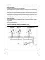
Figure 13.11 RS485 Bus Connections for Multiple DCells ....................................................................... 68
Figure 13.12 RS485 Bus Connections for Multiple DSC4-RS485 Versions............................................. 69
RS232 & RS485 Bus Converters ................................................................................................................. 70
Input Sensitivity Adjustment ......................................................................................................................... 70
Figure 13.13 Identifying the DCell ‘Rg’ Resistor ....................................................................................... 70
Fitting an External Temperature Sensor ...................................................................................................... 71
Figure 13.14 Identifying the DCell T+ and T- Track Cut ........................................................................... 71
Chapter 14 Troubleshooting......................................................................................................................... 72
No Communications ..................................................................................................................................... 72
Bad Readings............................................................................................................................................... 72
Unexpected Warning Flags.......................................................................................................................... 73
Problems with bus baud rate........................................................................................................................ 73
Recovering a ”lost” DCell/DSC..................................................................................................................... 73
Chapter 15 The VisualLink Application ....................................................................................................... 75
Figure 15.1 Communication & Parameter Test Page ............................................................................... 76
Figure 15.3 Instrument Settings Window .................................................................................................. 77
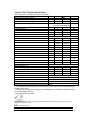
Chapter 16 Specifications............................................................................................................................. 78
Table 16.1 Technical Specifications ......................................................................................................... 78
Table 16.2 DSC Technical Specifications................................................................................................. 79
Mantracourt Electronics Limited DCell & DSC Version 2 User Manual Issue 1.3
3
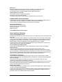
Chapter 1 Introduction
This chapter provides an introduction to DCell/DSC products, describing the product range, main
features and application possibilities.
Overview
The DCell and DSC products are miniature, high-precision Strain gauge Converters; converting a
strain gauge sensor input to a digital serial output. They allow multiple high precision
measurements to be made over a low-cost serial link. Outputs can be accessed directly by PLCs
or computers, or connected via various types of network, telephone or radio modem, all without
compromising accuracy.
Key Features
Ultra-miniature
The DCell ‘puck’ format can be fitted inside most load cell pockets, and similar restricted spaces.
The DSC cards are similarly very small, optimised for mounting as a component onto custom
PCBs.
High-precision
10ppm basic accuracy (equates to 17 bit resolution) with comparable stability – far exceeds
standard instrument performance.
Low-power
Low-voltage DC supply (8.5V min), typically 40mA per device. (including 350R strain gauge)
Adjustable sensitivity
Configured for standard 2.5mV/V full-scale strain gauges as supplied.
A single additional resistor configures the input between 1 and 100 mV/V full-scale.
Temperature sensing and compensation
Built-in temperature sensor and advanced 5-point temperature-compensation of measurement.
Linearity compensation
Advanced 7-point linearity compensation
Serial output
Lower-cost cabling, improved noise immunity, and longer cable runs with no accuracy penalty.
Device addressing allows up to 253 devices on a single bus, drastically reducing cabling cost and
complexity.
Two-way communications allow in-situ re-calibration, multiple outputs and diagnostics.
No separate measuring instruments needed.
Digital calibration
Completely drift-free, adjustable in-system and/or in–situ via standard communications link.
Two independent calibration stages for load cell- and system-specific adjustments.
Programmable compensation for non-linearity and temperature corrections.
Calibration data is also transferable between devices for in-service replacement.
Self-diagnostics
Continuous monitoring for faults such as strain overload, over/under-temperature, broken sensors
or unexpected power failure.
All fault warnings are retained on power-fail.
Multiple output options
Choice of 2 communications standards: RS232 or RS485.
Choice of 3 different protocols: ASCII, MODBUS or MANTRABUS, for ease of integration.
All variants provide identical features and performance.
Special Facilities
Output Capture Synchronisation
A single command instructs all devices on a bus to sample their inputs simultaneously, for
synchronised data capture.
Output Tare Value
4
Mantracourt Electronics Limited DCell & DSC Version 2 User Manual Issue 1.3
An internal control allows removal of an arbitrary output offset, enabling independent readings of
net and gross measurement values.
Cell Excitation Sensing
For increased accuracy and sensor malfunction detection
Dynamic Filtering
Gives higher accuracy on stable inputs, without increased settling time.
Programmable Output Modes
Output rate control enables speed/accuracy trade-off.
ASCII output version provides decimal format control and continuous output mode for ‘dumb
terminal’ output.
Unique Device Identifier
Every unit carries a unique serial-number tag, readable over the communications link.
Communications Locking
A private key locking scheme can restrict device access to the suppliers own software, giving
suppliers or systems integrators control over 3rd-party re-supply.
Communications Error Detection
An interruption of normal communications due to drop-outs or noise is detected as badly formatted
receive data, which triggers a diagnostic warning flag.
External Temperature Sensing
The internal temperature sensor can be replaced with an external device in contact with the
sensor, for improved accuracy (especially tracking changing temperature conditions).
Software Reset
A special communications command forces a device reboot, as a failsafe to ensure correct
operation.
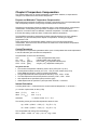
The Product Range
Devices are available in two physical formats.
The DCell (puck) products consist of a Digital Strain
gauge Signal Conditioner with RS485 bus output in an
ultra-miniature cylindrical “puck” format.
This is suitable for installation in very small spaces,
including load cell pockets.
External connections are made by wiring to solderpads.
The DSC (card) products are very similar to the DCell
but in a different physical form for mounting
standalone or on a board.
The DSC is also available with an RS232 output.
External connections are via header pins which can
plug into connectors, or be soldered to wires or into a
host PCB.
Which Device To Use
It is important to select the correct product for your application.
• First choose DCell or DSC based on your physical installation needs
• Choose the communications protocol depending on performance/integration requirements
• the RS232 output option may be simpler if your system only uses a single DSC card
Common Features
Both physical formats offer identical control and near-identical measurement performance
Both are available in all three output protocols: MODBUS, ASCII or MANTRABUS
Mantracourt Electronics Limited DCell & DSC Version 2 User Manual Issue 1.3
5
Differences
DCell (puck) has a 4 wire gauge connection for mounting very close to the sensor
The DSC (card) has a 6 wire gauge connection allowing a short cable run.
Only the DSC (card) is currently available with the RS232 output option
Special Aspects To Consider
The DCell fits neatly into a strain gauge pocket
The DSC lends itself to PCB mounting
The RS485 output version must be used for multiple devices on the same bus
Additional DSC Variants Available
A separate DSC variant is available with CANbus output, using a CANOpen-compliant protocol.
A DSC variant with 3 bits of digital i/o is available for simple control interfacing
(These variants are sufficiently different to require their own manuals)
Future Planned Versions
DCell (puck) form with RS232 output
DCell (puck) form with CANbus output
Ethernet connection
Radio connection
Contact Mantracourt for latest details.
Some Application Examples
Simple Distributed Measurement
Pressure loads are taken at a number of keys points in a manufacturing process, distributed over a
large area.
Each pressure sensor contains a DCell unit, and all the sensors are connected by a single cable
carrying power and RS485 communications. A central PC allows continuous display, monitoring
and logging of all values from a central control room. This displays a control-panel and current
display window, and logs information to an Excel spreadsheet for future analysis.
Further monitoring checks and displayed information can easily be added when required to the
system where up to 253 ‘nodes’ can be installed.
Low cost dedicated weighing station
A basic load cell weighing-pad device has a cable leading to a wall mounted weight display.
Digital Load Cell
Load cell products are offered with a high-precision digital communications option.
A DCell is fitted into the gauge pocket of each load cell in manufacture. During product testing,
each unit undergoes a combined load test and temperature cycle. Each unit is then programmed
with individually calculated gain, offset, linearity and temperature compensation tables. All units
perform to a very tight specification without the use of any trimming components.
High Reliability Load Sensing
A road bridge has a dedicated load monitoring and active control computer system. System
calibration adjustments are only established during construction, so sensors must be replaceable
without recalibration.
Each load monitoring point has a digital load cell fitted, with calibration values set during
construction. Self-diagnostics aid detection of failures.
When a failed load cell is replaced it will produce identical force measurements. The old load cell
set-up data values are programmed into the separate user-level calibration store in the unit, to
produce an identically performing replacement.
Remote radio weigher
A variety of lifting machines in a loading yard can be used with a weighing link to display weight in
tonnes on a remote hand-held readout.
A heavy duty strain gauge load-link is fitted with a battery-powered radio modem and DCell. The
independent handheld display unit communicates with the DCell over a transparent radio link,
providing a simple LCD readout and tare button operation.
6
Mantracourt Electronics Limited DCell & DSC Version 2 User Manual Issue 1.3
Load balance monitor
A lorry loading weighpoint monitors left/right load balance and sounds a warning if loading is too
uneven for safety.
A drive-on weighing platform is provided with load cells at each of four corners. Each cell is wired
to a DSC unit, and these are cabled to a 3rd-party LCD display and control unit, producing a
complete turnkey system. A digital I/O card is wired to the same bus to control the warning alarm.
Application software running on the control unit provides a % left/right balance readout with a
graphical tipping display, and a total weight indication.
The balance indication is calculated by comparing the different corner readings. If it exceeds a
programmed limit, a command to the I/O card turns the relay on.
Total weight is calculated by summing the individual results mathematically.
Automatic re-zeroing occurs when the total is near zero for more than a few seconds.
A control button enables a set-up mode for recalibration (protected by operator password), which
displays individual readings and total. Corner compensation can be checked by observing the
changing total as a weight is moved around. Simple button presses control two point recalibration
for any cell.
Weighing subsystem for process control
Several strain gauge loads are monitored as part of a larger data acquisition/monitoring system,
based around a high-speed Profibus network.
The load measurements occur in groups of physically related signals which relate to specific ‘area
modules’ along with a number of other measurements and control outputs.
The strain gauges are wired to DSC cards, controlled and interrogated via MODBUS protocol
commands on an RS485 bus. The DSCs and other 3rd-party MODBUS-compliant devices which
govern the area module are all connected to a single RS485 ‘spur’. The devices in each areamodule spur are controlled from the main Profibus backbone, using an off-the-shelf bus gateway
unit.
Mantracourt Electronics Limited DCell & DSC Version 2 User Manual Issue 1.3
7
Chapter 2 Getting Started with the Evaluation Kit
This chapter explains how to connect up a DCell/DSC for the first time and how to get it working.
For simplicity, this chapter is based on the standard DCell/DSC Evaluation Kit, which contains
everything needed to communicate with a puck or card from your PC.
It is advised that first time users wishing to familiarise themselves with the product use
Mantracourt’s Evaluation Kit. This provides a low cost, easy way to get started.
If you do not have an Evaluation Kit, the instructions in this chapter mostly still apply, but you will
need to wire up the device (and possible bus-converter) and have some means of communicating
with it. See Communications Protocols in Chapter 11 Communication as appropriate to the
protocol type.
See also Chapter 13 Installation for details on wiring up the device.
The Evaluation Kit
Contents
• An Evaluation PCB which comprises of
A 7 Way Screw Connector for the Strain Gauge
A 4 Way Screw Connector for Power & RS485 Comms
A 9 Way ‘D’Type for Direct RS232 Connection to PC
Link Headers for 4 Wire Strain Gauge Option (DCell)
Link Headers for RS232 or RS485 Comms Selection
Terminating resistor for RS485
•
•
•
•
An Evaluation DCell or DSC of your choice
A CD ROM containing VisualLink Evaluation Software
A 9 to 25 Way ‘D’Type Adaptor for the PC Comms Port
A 9 Way ‘D’Type Extension Lead
• For RS485 ONLY an RS232 to RS485 converter and connecting cable
• For RS232 ONLY a power connection cable
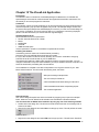
See the following diagram.
Figure 2.1 Evaluation Kits for the DCell & DSC
Evaluation Kit for the RS485, with the DCell
Evaluation Kit for the RS232 with the DSC
Other Things you will need
• A regulated power supply, capable of providing 10 -15V at 100mA (10v is minimum
requirement for RS485 converter)
• A PC running Windows 95 or above, with a spare RS232 communications port and 35Mb free
disk space
8
Mantracourt Electronics Limited DCell & DSC Version 2 User Manual Issue 1.3
and, ideally
• A strain gauge, load cell or simulator, 350-1000 ohms impedance.
(NOTE: the devices use ac excitation, so a dc mV source will not work)
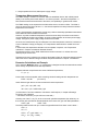
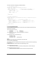
Checking the Device Protocol Type and Station Number
Before running the communications application, you should check both the protocol to use and the
device station number.
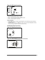
The product label shows the product code which determines the protocol and its serial number
which determines initial station number.
Example DCell label
98
Example DSC label
m
1000118851
‘D’Cell
For a DCell, the Product Code is one of the following 3 types
DLCPKASC
ASCII output
DLCPKMAN
MANTRABUS output
DLCPKMOD
MODBUS output
For a DSC card, the Product Code is one of the following 6 types
RS485 output card with ASCII protocol
DSC4AS
RS485 output card with MANTRABUS protocol
DSC4MA
RS485 output card with MODBUS protocol
DSC4MB
RS232 output card with ASCII protocol
DSC2AS
RS232 output card with MANTRABUS protocol
DSC2MA
RS232 output card with MODBUS protocol
DSC2MB
NOTE: For evaluation purposes, the electrical output standard RS485 or RS232 is not important:
Your kit should contain the correct equipment to connect the device to a PC.
The product code should match your original order.
The serial number of the device is also shown.
The station number of a new DCell/DSC device is set up to have the same
last 2 digits as its serial number
E.G. 817752 gives station 52, while 103800 gives station 100.
(N.B. this is only the factory set value; and its value changed by a previous user)
Make a note of both the protocol and station number now. The communications application needs
to be told both the protocol to use and the station number to communicate with.
Connecting Up The Evaluation Kit For RS485
Connect the PC using the 9 way ‘D’Type to the RS232/RS485 converter. Plug the cable provided
into the converter and connect the other end to the 4 way screw connector on the PCB using the
colour codes indicated on the PCB ident.
Ensure LK4 & LK5 are set to pins 1 & 2. Fit LK3 which terminates the RS485 comms. Connect the
power cable to your power supply, which has been set to deliver between 10 & 15 volts, then
switch on.
Mantracourt Electronics Limited DCell & DSC Version 2 User Manual Issue 1.3
9
Figure 2.2 DCell - RS485 Versions Evaluation Kit Communications
Figure 2.3 DSC4-RS485 Versions Evaluation Kit Connections
Connecting Up The Evaluation Kit For RS232
Connect the supplied power cable (Red & Black twisted) to the 4 way screw noting the colours
indicated on the PCB.
Connect the 9 way ‘D’Type extension lead to the J1 of the evaluation board marked (RS232) and
the other end to the comms port of the PC.
Ensure LK4 & LK5 are set to pins 3 & 2 again see PCB indent for the markings of these links.
Now connect power cable to your power supply, which has been set to deliver between 10 & 15
volts, and switch on.
10 Mantracourt Electronics Limited DCell & DSC Version 2 User Manual Issue 1.3
Figure 2.4 DSC2-RS232 Versions Evaluation Kit Connections
Note that if your PC serial port has a 25 way serial port connector, you should use the 9 to 25 way
‘D’ type adaptor provided to connect to the evaluation hardware.
Installing VisualLink
The DCell/DSC evaluation communications application is written for the VisualLink environment.
VisualLink is Mantracourt’s own rapid development software platform for PC SCADA applications.
It provides communications drivers for the DCell/DSC products (amongst many others). An
evaluation copy is provided on CD-ROM with the DCell/DSC Evaluation Kit.
Uninstall any previous versions of VisualLink before proceeding.
Install the VisualLink demonstration application by inserting the CD in the CD ROM drive. This
should start the ‘AutoRun’ process, unless this is disabled on your computer.
(If the install program does not start of its own accord, run SETUP.EXE on the CD by selecting
‘Run’ from the ‘Start Menu’ and then entering D:\SETUP, where D is the drive letter of your
CD-ROM drive).
The install program provides step-by-step instructions. The software will install into a folder called
VisualLink inside the Program Files folder. You may change this destination if required.
After installation you may be asked to restart the computer. This should be done before proceeding
with communications.
For further information, refer to Chapter 15 The VisualLink Application
Running the VisualLink Evaluation Application
Having installed VisualLink, you can now run the special evaluation application, which the rest of
this chapter is based around.
From the windows ‘Start’ button, select Programs, then VisualLink, select Design Examples. This
opens a folder, double click on ‘DSC & DCell Evaluation.vld’.
Will open the design example folder
The on-line help for VisualLink
A brief animated tutorial about adding an instrument
A brief animated tutorial about manipulating objects
The VisualLink application
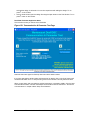
The following window should appear:–
Mantracourt Electronics Limited DCell & DSC Version 2 User Manual Issue 1.3
11
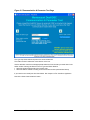
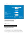
Figure 2.5 Communication & Parameter Test Page
The ‘type’ drop-down selects the protocol to communicate with.
The ‘station number’ selects the correct device on the bus.
Use the selection controls to make appropriate selections, from the data you noted down in the
earlier section Checking the Device Protocol Type and Station Number
• Select the protocol appropriate to the product code
• Select the station-number according to the device serial number (as described above)
If you need to use a serial port other then COM1. See Chapter 15 The VisualLink Application
Now hit the ‘Start Communications’ button…
12 Mantracourt Electronics Limited DCell & DSC Version 2 User Manual Issue 1.3
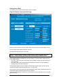
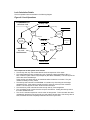
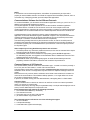
Viewing Device Data
The following, main ‘Communications Page’ should now appear
Figure 2.6 Device Communications Page
At the top are shown the device type, serial number and current communications station number.
The main device output values are shown on the left.
The diagnostics flags are shown on the right
If there is a communications problem, a separate ‘Error’ window will appear after a few
seconds – check all settings, and Chapter 14 Troubleshooting for additional advice.
Once communications are established, the screen displays current information values read from
the DCell/DSC device :–
• The ‘SOUT’ value is the main device output –this is probably currently near zero as there is no
input connected.
• The ‘TEMP’ value is the internal temperature measurement reading – this will probably be
changing slowly as the device warms up.
The application refreshes these two displays at a reasonably fast rate, about 3 times a second,
while the other data is read less frequently (every 1 or 2 seconds).
On the right, the ‘FLAG’ value shows the device diagnostic warning flags. Individual bits of this 16bit parameter register represent specific warning conditions.
This value is generally zero in normal use, but at present will have at least bits 15 and 1 set (value
32768+2=32770).
Mantracourt Electronics Limited DCell & DSC Version 2 User Manual Issue 1.3
13
The application also displays the current bit settings as individual indicators: Bits 15 and 1 are
shown as the REBOOT and EXCOR flag indicators.
REBOOT means the device has been reset (usually powered down).
EXCOR means the excitation measurement is above a warning ‘high’ limit (“EXCitation OverRange”): This is a sensor high-impedance warning, i.e. the input gauge is broken or disconnected.
If you now hit the ‘Clear All’ button next to the FLAG value, the REBOOT warning (and any others)
should clear, but the EXCOR flag will remain set (assuming that there is still no load cell
connected), and the FLAG value will be 2.
Now you have successfully established communications with your evaluation device, future
chapters concentrate on specific feature areas.
14 Mantracourt Electronics Limited DCell & DSC Version 2 User Manual Issue 1.3
Chapter 3 Basic Setup and Calibration
This chapter explains the most common setup and maintenance operations for operating
DCell/DSC devices. This includes initial calibration, and communications settings.
Connecting a Load Cell
You can now connect a strain gauge bridge, load cell or simulator to the DCell/DSC.
A suitable strain gauge should have an impedance of 350-1000ohms and (at least for now) a
nominal output of around 2.5mV/V.
NOTE: You can’t just simulate a cell input with a small voltage.
This is because DCell/DSC devices use an AC bridge excitation, so the input is an AC signal
changing in phase with the excitation.
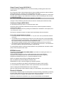
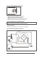
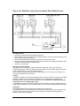
Note the following
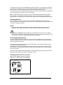
1. If using the DCell or a 4 wire strain gauge then ensure LK1 & LK2 are fitted. Connections to
+Sen & -Sen will not be made.
2. The cable length from strain gauge to evaluation PCB should be as short as possible and not
exceed 3 meters.
3. The screen should be connected to the body of the load cell and terminated at ‘CHASS’.
Figure 3.1 Evaluation Board Sensor Connections
-Exc
LK1
Evaluation
Board
(6 wire DSC only)
-Exc
Rg
Rg
-Sen
-Sig
+Sig
Strain
Gauge
-Sig
+Sig
(6 wire DSC only)
LK2
+Sen
Rg
Rg
+Exc
CHASS
+Exc
Once you have connected the load cell, you should see ‘believable’ output values on the main
reading “SOUT” indicator, that change with the input level between about –100.0 and +100.0.
The readings are scaled in “percent full-scale”, i.e. it reads 100.0 for a 2.5mV/V input.
If you hit the ‘Clear All Flags’ button, the EXCOR warning flag should now clear, and the FLAG
value will just be zero.
Adjusting the System Calibration
The values obtained so far are simple ‘electrical’ readings, in %-full-scale (where 100% is the basic
2.5mV/V output level).
These are produced by the device ‘electrical’ calibration, which is factory-fixed to within about 0.2%
accuracy.
This inbuilt calibration cannot be changed, however the device also contains separate useradjustable calibration controls. These allow you to rescale the output value to read in units of your
choice, and to calibrate precisely to your load cell / system hardware for much more precise
results.
To see this, from the main ‘Communications’ page, hit the ‘System Calibration’ button
Mantracourt Electronics Limited DCell & DSC Version 2 User Manual Issue 1.3
15
The following page should now appear :–
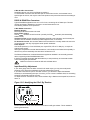
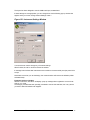
Figure 3.2 System Calibration Page
The boxes labelled SOFS, SGAI, SMIN and SMAX show the current values of control parameters
stored in the device.
To change a setting, just click in the relevant box and enter the new value. The new value is sent
to the device immediately.
This application page shows how the SOUT output is produced from the basic CELL reading value
by the following steps
1. The input is the CELL reading value
2. This then has SOFS (the system offset) subtracted from it
3. The result of this is multiplied by SGAI (the system gain)
4. After applying GAIN the result is limited to the range SMIN..SMAX (system minimum to system
maximum)
5. This gives the new SOUT output value
The system over-range flags are also shown (SYSUR,SYSOR = system under-range / overrange): If the scaled result was bigger than SMAX or smaller than SMIN, then the SYSOR or
SYSUR flag is set.
NOTE:- SMIN & SMAX also clamp the output SOUT to exceeded value!
Try changing the SOFS and SGAI parameters to different values :–
The SOFS parameter is used to remove the cell output offset.
E.G. If CELL reads 0.1253 when the load cell is unloaded, set SOFS=0.1253 to make SOUT=0
with no load.
The SGAI parameter scales the results, so changing the output units.
E.G. if you have a 2.5mV/V output, 5 tonne load cell, then the CELL output should be 100 for
a nominal 5-tonne load. So setting SGAI=0.05 causes the cell to read approximately in
16 Mantracourt Electronics Limited DCell & DSC Version 2 User Manual Issue 1.3
tonnes
Note that when you change SGAI, you change the output ‘units’, so SMIN and SMAX may also
need to be adjusted.
E.G. if, in the previous example, you wanted an output in Kg, you would set SGAI=5.0. But
the valid output range will then be ±5000 (Kg), so you also need to set SMIN=-5000 and
SMAX=5000 as well –otherwise the output will still be limited to ±100.
The boxes show the current values of parameters in your device: The applications page reads
data from the device to display the values, and allows you to enter new values which are then sent
back to the device. It thus acts as a ‘window’ on the data within the device you are currently
communicating with.
To return to the previous page, just hit the ‘Main Comms Page’ button.
Device Communications
Most interactions with DCell/DSC devices actually involve reading and writing ‘parameter’ values,
• Device outputs are read from ‘read-only’ parameters
• Control values (such as the calibration controls above) are read/write parameters
• Some fixed values (such as device serial-number) are also read-only
However, some commands can simply cause a one-off action to be performed, e.g. the SNAP
command takes a ‘snapshot’ sample of the current output value (see in Chapter 10 Additional
Software Features), and the RST command causes a device reboot (see Changing Device
Communications Settings, below).
The commonest use of DCell/DSC devices in an overall system involves several devices on one
bus, with a ‘host’ controller reading the main output value from each device in turn. Less
frequently, the host also checks the devices’ warning flags. Other, occasional activities may use
other commands.
In this situation, the permanently-stored control parameters for calibration and communications
setup are normally set up in the initial installation process, and then never (or rarely) touched.
WARNING: Finite Non-Volatile Memory Life
The DCell and DSC use EEPROM-type memory as the storage for non-volatile controls (i.e. all the
settings that are retained even when powered down).
The device EEPROM itself is specified for 100,000 write cycles (for any one storage location).
Therefore –
When automatic procedures may write to stored control parameters, it is important to make
sure this does not happen too frequently.
So you should not, for example, on a regular basis adjust an offset calibration parameter to zero
the output value. However, it is reasonable to use this if the zeroing process is initiated by the
operator, and won’t normally be used repeatedly.
For the same reason, automatically cancelling warning flags must also be implemented with
caution: It is okay as long as you are not getting an error recurring repeatedly, and resetting it
every few seconds.
Setting a Precise Calibration
NOTE: the full calibration facilities are considerably more complex than the basic
calculations described here. See Chapter 5 Readings Processing and Calibration for fuller
details.
In order to get correct measurement values from a device, you need to establish precise values for
the calibration controls. This generally depends on the combined performance of the measuring
device, load cell and (often) the mechanical system it is installed in.
Mantracourt Electronics Limited DCell & DSC Version 2 User Manual Issue 1.3
17
Once you have worked out correct values for SGAI and SOFS, these values are simply written into
the parameters, as shown above. This then gives precise readings in the required output units.
The SMIN and SMAX controls are then set to the expected normal range of the output value.
(One of the advantages of digital calibration is that the results of changing the calibration are
always precisely known –i.e. you can calculate exactly what results you will get with a particular
change to the calibration setup, there is no ‘cut and try’ needed)
If you have a load cell connected, and a suitable test weight, you can calibrate the cell in the
simplest way as follows
1. Run up the VisualLink DCell/DSC Evaluation Design Application, and select the ‘System
Calibration’ page, as above
2. Set SGAI back to the default 1.0, SOFS to 0.0 and SMIN/SMAX to –/+100.0
3. Remove all load so the inputs see’s the desired ‘zero’ calibration point and allow to settle
4. Note the CELL reading value, and copy this into SOFS.
SOUT should then read zero.
5. Apply your test weight, and allow to settle, ideally this would be about full range for best
accuracy over the measurement range.
6. Take the known weight of your test weight (in the required engineering units), and divide by the
current SOUT value – i.e. calculate (weight)/(SOUT) Put this value into SGAI.
7. Set SMIN and SMAX to an appropriate output value range.
SOUT should now show the value of the test weight, as required
The next section briefly reviews different methods of establishing the calibration values.
Calibration Methods
There are a number of ways of establishing the correct control values
Method 1 - Nominal (data sheet) performance values
This is the simplest method, where the given nominal mV/V sensor output is used to calculate an
approximate value for SGAI (as described in the above example).
E.G. a 50 kN (i.e. approx 5-tonne) load cell has nominal sensitivity of 2.2mV/V full-scale.
The standard DCell/DSC sensitivity is 2.5mV/V, giving an output value of 100, so to get 50.0
for an input of 2.2mV/V, we set SGAI to 50/100*(2.5/2.2)≈0.568182.
( N.B. 6 figures is a suitable accuracy to work to )
It is also useful to set SMIN/SMAX=–/+50.0, to show when the input goes out of the normal
range, because the electrical signal will now never exceed the normal range.
Method 2 - Device Standard (Calibration) Values
With some load cells you may have a manufacturer’s calibration document. This gives precise celloutput gain and offset specifications for the individual cell. These values can be used to set the
SGAI and SOFS values to be used.
E.G. a 10 tonne load cell has a calibration sheet specifying 2.19053mV/V full-scale output,
and -0.01573mV/V output offset.
SOFS is set to the input offset in %-of-2.5mV/V, which is –0.01573/2.5*100 ≈ –0.629200
SGAI is set to (10/100)*(2.5/2.19053) ≈ 0.114128
SMAX and SMIN can be set to 10.0 and –0.1 (if negative loads are not expected in this case)
NOTE:
Methods 1 and 2 require no load tests. This means that systematic installation errors cannot be
removed, such as cells not being mounted exactly vertical. The accuracy is also limited by the
DCell/DSC electrical calibration accuracy, which is about 0.2%.
The remaining methods require testing with known loads, but are therefore inherently more reliable
in practice, as they can remove unexpected complicating factors relating to installation.
Method 3 - Two-Point Calibration Method
This is a simple in-system calibration procedure, and probably the commonest method in practice
(as in the previous example).
Two known loads are applied to the system, and reading results noted, then calibration parameters
are set to provide exactly correct readings for these two conditions.
18 Mantracourt Electronics Limited DCell & DSC Version 2 User Manual Issue 1.3
E.G. a 10kN (1-tonne) load cell has a CELL reading of +0.120721 with no load, and -87.2077
with a known 100Kg test-weight.
To calibrate this to read in a –1.0 to +1.0 tonne range, set SOFS=0.120721, SGAI=0.1/(87.2077 – +0.120721)≈–0.00114510 and SMAX/SMIN=+/-1.10
NOTE:
The usual method for weighing systems is to make point (1) the unloaded state, which should read
zero, and point (2) with a known test weight on, which should read the value (in required units) of
the test weight. This approach is simpler, because you can remove the offset first, as explained in
the previous section.
Method 4 - Multi-point Calibration Test
For ultimate accuracy to a whole series of point measurements may be taken to determine the best
linear scaling of input output: Effectively, a ‘best line’ through the data is then chosen, and the
calibration is set up to follow the line.
Testing of this sort is also used to establish linearity corrections, and similar tests at different
temperatures are used to set up temperature compensation (see Chapter 6 Temperature
Compensation and Chapter 7 Linearity Compensation).
Changing Device Communications Settings
This section explains the other most commonly used settings – those used to control device
communications.
The device bus standard and protocol type are specified by the product code, and fixed during
manufacture. However, the communications ‘station number’ (bus address) and baudrate are
programmable via communications parameters. Care is needed when changing these, to avoid
losing communications with the device, so this section demonstrates how to do this correctly.
If you lose all communications with the device, see Chapter 14 Troubleshooting to solve the
problem.
The section also shows you how to adjust the device output rate, and how this affects the output
readings.
From the main ‘Device Communications’ page in the VisualLink evaluation application, hit the
‘Control Settings’ button.
The following page should now appear :–
Mantracourt Electronics Limited DCell & DSC Version 2 User Manual Issue 1.3
19
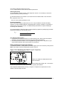
Figure 3.3 Control Settings Page
The SOUT and FLAG info are shown here for reference only.
The RATE, STN and BAUD settings control
output rate, station number and comms baudrate.
The ‘RST’ button sends a device reboot command.
This is needed for changes to RATE, STN and BAUD to take effect.
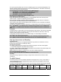
Output Rate Control
The RATE parameter is used to select the output update rate, according to the following table of
values –
RATE value
update rate (readings per second)
0
10
1
1
2
100
The normal rate is 10Hz (RATE=0): The other settings give a different speed/accuracy trade-off.
Invalid RATE values are treated as if it was set to 0.
To change the output rate
1. Set RATE to the new value
2. Hit the ‘RST’ button to reboot the device
3. Wait for 3 seconds for the reset procedure to complete and measure cycle to start
The value displays will ‘freeze’ for 2-3 seconds, as VisualLink interrupts communications for a
while whenever a device is rebooted, to avoid spurious errors when the device does not respond.
With RATE set to 1, you should be able to see the SOUT update rate slow to once a second, and
the noise level should also noticeably decrease.
20 Mantracourt Electronics Limited DCell & DSC Version 2 User Manual Issue 1.3
With RATE=2, you won’t see any difference in rate because VisualLink can’t display the results
much quicker than 10 a second, but increased noise can be seen.
All the main-reading output values are updated at this rate. See Figure 5.1 Readings Processing –
for an overview of readings processing.
Baud Rate and Station-Number Controls
Station Number, STN
The STN parameter controls the ‘station number’, which specifies the device address for bus
communications.
As supplied, devices have the station-number set according to the device serial number, as
described previously in Checking the Device Protocol Type and Station Number.
To change the station number of your device
1. First set STN to a suitable new value (making sure that no other device of the same number is
also connected!)
2. Now hit the ‘RST’ button to reboot (needed before the device begins to use the new value)
3. Wait for a VisualLink ‘Errors’ window to appear.
(because it is no longer getting responses to commands addressed to the old number)
4. Return to the startup page, by hitting the ‘Restart Comms’ button
5. Clear the errors, and close the Errors window
6. Select the new Station Number in the dropdown list
7. Hit ‘Start Communications’ button again. You should now find you can talk to the device again
To connect multiple devices on the same bus, it is first vital to set all the station numbers to
different values.
This is because if two devices with the same station number are connected to the same bus, it is
not possible to talk to them individually: So in particular, you cannot correct the problem by
changing the station number of one of them!
If a bus connects to two devices with the same station number, the only solution is to remove one
of them and connect it to a one-to-one link to reprogram it.
NOTES:
• The valid range of STN depends on the protocol, but it is always at least 1-253.
• All the protocol types have a ‘bus address’ type device identifier, which is known as the ‘station
number’ for MANTRABUS, ‘address’ for ASCII and ‘node id’ for MODBUS.
• The valid ranges for different protocols are: 1-253 for MANTRABUS, 1-999 for ASCII and 1-255
for MODBUS.
• In all cases, if STN is set outside the valid range, it behaves as if set to a default of 1.
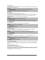
Baudrate Control, BAUD
The BAUD parameter is a read/write byte value specifying a standard communications baudrate
according to the following table –
BAUD value
1
2
3
4
5
baud rate
2400
4800
9600
19200
38400
(bps)
BAUD can only take the values shown above. If set <1 or >5, the baud rate defaults to 9600.
Warning: When changing this setting it is possible to lose communication with the device.
As well as keeping track of the correct baudrate, it is also essential in this case to be sure
that your hardware supports the rate you are changing to.
The evaluation kit supports all possible DCell/DSC baudrate settings.
When changing baudrates, you should not see any noticeable difference, except maybe slight
changes in responsiveness when changing parameter values. However, if you design your own
communications applications (with VisualLink, or otherwise), higher baudrates will allow faster
readout rates etc.
Mantracourt Electronics Limited DCell & DSC Version 2 User Manual Issue 1.3
21
Lowering the baudrate is generally only needed where very long cable runs are used, to improve
communications reliability.
To change the baudrate, follow a similar sequence to changing the STN value
1. First set BAUD to the new value
2. Now hit the ‘RST’ button to reboot (needed to make the device start using the new value)
3. Wait for the VisualLink ‘Errors’ window to appear
4. Return to the startup page, by hitting the ‘Restart Comms’ button
5. Clear the errors, and close the Errors window
6. Hit the ‘Change Comms Settings’ button: A new popup window appears
7. Select the new VisualLink communications baudrate with the popup menu controls
8. Hit ‘Ok’ to confirm and hide the window
9. Hit ‘Start Communications’ button again. You should now find you can talk to the device again
22 Mantracourt Electronics Limited DCell & DSC Version 2 User Manual Issue 1.3
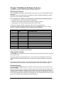
Chapter 4 Summary of Software Features
This chapter gives a complete overview of all the software functions.
Each item has only a brief description here, consult the references for detailed information.
User Calibrations
The devices have sophisticated digital calibrations, which can be adjusted via communications.
See Chapter 5 Readings Processing and Calibration.
Diagnostic Warnings
Checks are continually made on correct operation, and warning flags record any problems found.
See Chapter 6 Self Diagnostics.
Temperature Compensation
An internal temperature measurement can be used to correct for sensor drifts with temperature.
See Chapter 6 Temperature Compensation.
Linearity Compensation
Corrections can be applied to correct for non linearities in the input measurement.
See Chapter 7 Linearity Compensation
Communications Lock
A ‘security’ scheme enables a supplier to ensure that devices they sell can only be used with their
software, and vice-versa.
See Chapter 9 Device Locking.
Factory Calibration
The calculations for the basic electrical reading and the temperature measurement are described
in Electrical Calibration and Temperature Calibration in Chapter 10 Additional Software Features.
Input Filtering
The input Electrical calibration processing involves a dynamic filtering technique, explained in
Chapter 10 Additional Software Features.
Result Snapshot
Multiple inputs can be sampled simultaneously with a single bus command.
See Reading Snapshot in Chapter 10 Additional Software Features.
Continuous Output
(ASCII protocol only): Devices can be made to transmit continuously for output on slave display.
See Continuous Output in Chapter 10 Additional Software Features.
Output Formatting
(ASCII protocol only): The decimal formatting of the output value is adjustable.
See Output Format Control in Chapter 10 Additional Software Features.
Output Tracking
A flag mechanism allows every output result to be sampled once and once only.
See Output Update Tracking in Chapter 10 Additional Software Features.
Output Selection
The main output can be switched between different internal values.
See SOUT Output Selection in Chapter 10 Additional Software Features.
Information Parameters
The device serial-number and software version can be read back over the communications.
See Informational Parameters in Chapter 10 Additional Software Features.
EEPROM access
Special commands to access internal storage are used to adjust the factory calibration.
See EEPROM Controls in Chapter 10 Additional Software Features. Software Reset
A ‘reboot’ command is also used to implement communications settings changes.
See Software Reset in Chapter 10 Additional Software Features.
Mantracourt Electronics Limited DCell & DSC Version 2 User Manual Issue 1.3
23
Chapter 5 Readings Processing and Calibration
This chapter gives a complete account of the calibration controls and processing of input readings
except for the linearity-and temperature-compensation processes (which have their own chapters
later on).
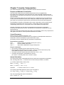
Main Reading Calculations
The following figure shows a simplified view of the whole of the readings processing calculations,
omitting the compensation calculations (see Figure 5.2 for the complete version).
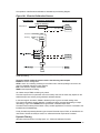
Figure 5.1 Readings Processing – Main Features
‘Electrical’ Outputs
‘Cell’ Calibration
‘System’ Calibration
ELEC
TEMP
−
CRAWUR
CRAWOR
COFS
−
SOFS
×
SGAI
×
CGAI
≥
CMIN
≥
SMIN
CMAX
≤
SMAX
≤
SRAWUR
SRAWOR
SRAW
−
CELL
SYSN
This ‘chain’ of calculations is performed on every input reading.
The named values shown in the boxes are all output parameters, which can be read back over the
comms link.
These calculations are updated continually, at the update rate set by the RATE control (see Output
Rate Control in Chapter 3 Basic Setup and Calibration).
The diagram shows three separate calibration stages, called the ‘Electrical’, ‘Cell’ and ‘System’.
This allows independent calibrations to be stored for the device itself, the load cell and the installed
system characteristics –
Electrical
The ‘Electrical’ calibration produces corrected electrical readings from the internal measurements.
This is factory-set by Mantracourt during the production process.
(There are effectively three electrical calibrations, one for each output rate setting)
The main outputs from this are –
• ELEC is the raw electrical output, in “% full scale” units.
• TEMP is a device temperature measurement, in °C.
There are also two flags, ECOMUR and ECOMOR (not shown on the diagram), which indicate an
input electrical under- or over-range.
The electrical calibration is not covered in detail here, because it normally never changes after
manufacture, and is not controlled by communications parameters.
(A fuller account is given in Electrical Calibration in Chapter 10 Additional Software Features)
24 Mantracourt Electronics Limited DCell & DSC Version 2 User Manual Issue 1.3
Cell
The ‘Cell’ calibration converts the raw electrical output into a cell-force reading.
This can be used by an OEM sensor manufacturer to provide a standard, calibrated output in force
units, which could be based on either typical or device-specific calibration data.
(This stage also includes the temperature- and linearity-corrections, not covered here)
The outputs from this are
CELL is a load cell force reading in “Force” units (e.g. kN)
CRAWUR and CRAWOR are two flags indicating under or, over range for the force measurement.
System
The ‘System’ calibration converts the Cell output into a final output value, in the required
engineering units.
This is normally be set up by a systems installer or end user, to provide whatever kind of output is
needed, independently of device-specific information in the Cell calibration.
(Making this split allows in-service replacement without re calibration).
The outputs from this are
• SRAW is a re-scaled and offset adjusted output
• SYS is the final output value, after removing a final user output offset value (SZ) from SRAW
• SRAWUR and SRAWOR are output warning limit flags.
In practice, SRAW and SYS can be used to represent something like gross and nett values.
Results Value Scaling
Both the Cell and System calibrations are simply linear rescaling calculations –i.e. they apply a
gain and offset.
In both cases, four parameters define the scaling, offset and min and max limit values. These
calculations are applied in the following way:
Output = (input – OFS) × GAI
Output = min(output, MAX)
Output = max(output, MIN)
(In addition, if the value exceeds either limit, one of two dedicated error flags is set)
The control parameters thus have the following characteristics: –
• OFS is the input value that gives zero output, set in “input units”
• GAI is the multiplying factor, set in “output-units per input-unit”
• MAX and MIN are output limit values, set in “output units”
The units and functions of the main scaling controls can thus be summarised as –
Cell Calibration
ELEC value offset (ELEC value giving CELL=0)
[%fs]
COFS
CELL/ELEC gain factor
[force/%fs]
CGAI
Minimum value for CRAW
[force]
CMIN
Maximum value for CRAW
[force]
CMAX
System Calibration
CELL value offset (CELL value giving SRAW=0)
[force]
SOFS
[eng/ force] SYS/CELL gain factor
SGAI
Minimum value for SRAW
[eng]
SMIN
Maximum value for SRAW
[eng]
SMAX
SRAW value offset (SRAW value giving SYS=0)
[eng]
SZ
(where “%fs” is “per-cent full scale”, “force” is force units, and “eng” is engineering units)
Mantracourt Electronics Limited DCell & DSC Version 2 User Manual Issue 1.3
25
The SOUT Main Output Value
The “main” output value, SOUT, is normally an identical copy of the final system output, SYS.
In fact, however, SOUT can be ‘selected’ to track any of a whole group of different output
parameters. Details for this are given in SOUT Output in Chapter 10 Additional Software Features.
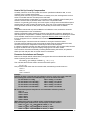
A Complete Picture of Readings Processing
For completeness, the following diagram shows a total overview of the calibration processes
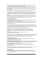
Figure 5.2 Readings Processing – Full
Electrical Outputs
Cell Calibration
System Calibration
ELEC
TEMP
CTOx(CTx)
−
−
SOFS
COFS
−
×
SGAI
1+CTGx(CTx)
×
CGAI
×
≥
SMIN
CMIN
≥
≤
SMAX
CMAX
≤
CRAW
CLKx(CLXx)
SRAW
−
+
SYS
CELL
SOUT
The detailed operation of the ‘Cell’ calibration stage, as shown above, as follows
• The raw ‘ELEC’ input is rescaled by the ‘Cell’ controls and temperature compensated (based on
current TEMP value) to give the CRAW value.
• CRAW is then linearity-compensated to give the final CELL output
NOTES:
1. Temperature-compensation is integrated with the basic cell scaling calculations, so there is no
‘uncompensated cell output’ value available.
2. The cell range limits, CMIN and CMAX are applied to the CRAW result, not the linearised value
3. The system range limits are applied to SRAW, not SYS, so the range errors SYSUR and
SYSOR are independent of the SZ setting.
This more complete picture is used for the discussion of the compensation facilities in the following
chapters.
Calibration Parameters Summary and Defaults
The various control parameters are listed for each stage.
This also includes the compensation parameters, not covered in this chapter, but shown in Figure
5.2 Readings Processing – Full
The ‘default’ values shown set the device back to its nominal default calibration (%-full-scale
output)
26 Mantracourt Electronics Limited DCell & DSC Version 2 User Manual Issue 1.3
Cell Control Defaults
Command
Action
COFS
basic cell offset
CGAI
basic cell gain
CTN
number of temp points
CT1..5
temp point values
CTO1..5
offset adjusts
CTG1..5
gain adjusts
CMIN
craw min limit
CMAX
craw max limit
CLN
number of linearity points
CLX1..7
linearity raw-value points
CLK1..7
linearity adjusts
Default Values
0.0
1.0
2
0.0, 25.0, 0,0…
0.0, 0.0, 0,0…
0.0, 0.0, 0,0…
–150.0
+150.0
2
0.0, 100.0, 0,0…
0.0, 0.0, 0,0…
System Control Defaults
Command
Action
SOFS
basic offset
SGAI
basic gain
SMIN
raw min limit
SMAX
raw max limit
SZ
output zero offset
Default Values
0.0
1.0
–150.0
+150.0
0.0
Two-Point Calibration Calculations and Examples
Values for both the Cell and System calibrations can be set up in any of the ways described under
Calibration Methods in Chapter 3 Basic Setup and Calibration.
Examples are given here for two-point calibration, as this is by far the most common method.
Cell Calibration
The scaling parameters are COFS, CGAI, CMIN and CMAX –
COFS is in ‘%’ (nominal percent-full-scale from electrical calibration)
CGAI is in ‘cell-units per %’
CMIN, CMAX are in cell units.
The cell output calculation is (in the absence of temperature and linearity corrections) –
CELL = (ELEC – COFS) × CGAI
If we have two electrical-output (ELEC) readings for two known force loads, we can convert the
output to the required range. So if –
test load = fA Æ ELEC reading = cA
test load = fB Æ ELEC reading = cB
– then calculate the following gain value
CGAI = (fB – fA) / (cB – cA)
and the offset is
COFS = cA – (fA / CGAI)
The outputs should then be CELL = fA,fB true force values, as required.
System Calibration
For system calibration, the arrangement is very similar
The parameters are SGAI, SOFS, SMIN and SMAX. So –
SOFS is in cell units
SGAI is in ‘engineering units per cell unit’
SMIN, SMAX are in engineering (output) units.
The system calculations are —
SRAW = (CELL – SOFS) × SGAI
SYS = SRAW – SZ
Mantracourt Electronics Limited DCell & DSC Version 2 User Manual Issue 1.3
27
If we have two cell-output (CELL) readings for two known test loads, we can convert the output to
the required range. So if –
test load = xA Æ CELL reading = cA
test load = xB Æ CELL reading = cB
– then we calculate the following gain value
SGAI = (xB – xA) / (cB – cA)
and then the offset
SOFS = cA – (xA / SGAI)
The outputs should now be SRAW = xA, xB true load values, as required.
Example:
A 2500Kgf load cell installation is to be calibrated by means of test weights.
The cell calibration gives an output in Kgf ranging 0–2000.
A system calibration is required to give an output reading in the range 0–1.0 tonnes.
Calculations
Take readings with two known applied loads, such as –
For test load of xA = 99.88Kg :
CELL reading cA = 100.0112
For test load of xB = 500.07Kg
:
CELL reading cB = 498.7735
Calculate gain value. In this case put SGAI = (xB – xA) / (cB – cA)
= (0.50007 – 0.09988) / (498.7735 – 100.0112)
≈ 0.001003580 = 1.003580•10-3
Calculate offset value. In this case SOFS = (cA – xA/SGAI)
= (100.0112 – (0.09988 / 1.003580•10-3))
≈ 0.487495
Set SMIN, SMAX to include the expected output range
say SMAX = +1.0, and SMIN = –0.1 to allow for small negative loads
Check
Putting the values back into the equation, results for the two test loads should then be —
For x = 99.88Kg, CELL = 100.0112, so
SRAW ≈ (100.0112 – 0.487495) × 1.003580•10-3 ≈ 0.0998799
For x = 500.07Kg, CELL = 498.7735, so
SRAW ≈ (498.7735 – 0.487495) × 1.003580•10-3 ≈ 0.5006987
The remaining errors are due to rounding the parameters to 7 figures.
Internal parameter storage is only accurate to about 7 figures, so errors of about this size
can be expected in practice.
28 Mantracourt Electronics Limited DCell & DSC Version 2 User Manual Issue 1.3
Chapter 6 Temperature Compensation
This chapter explains how to use the Temperature Compensation facilities, to compensate for
changes in the measurement with ambient temperature.
Purpose and Method of Temperature Compensation
Most measurement methods are affected by changes in temperature, and (uncompensated) load
cells are especially sensitive, having a large overall temperature coefficient.
Temperature compensation adjusts the measured value in a way that depends on a temperature
measurement, so that (ideally) the output does not depend on the current temperature.
In practice, it is usual to refer to a calibration ‘reference’ temperature: The ideal output value is
then what the reading ‘would have been’ if made at the reference temperature.
The DCell/DSC temperature compensation facilities make adjustments to the ‘Cell’ calibration
parameters (i.e. gain and offset) which depend on temperature, according to a digitally
programmed curve.
These adjustments are automatically applied, based on the current device temperature
measurement. With some care, this can remove the need for the usual electrical compensation
components altogether.
Control Parameters
The temperature compensation parameters define a pair of lookup tables that contain adjustments
to the cell calibration gain and offset over temperature.
The parameters concerned are the following
[-]
number of temperature table points
CTN
indicated TEMP value at table point
CT1…CT5
[°C]
CTO1…CTO5 [ppm-fs]
ELEC offset (×104) adjustment at table point
CTG1…CTG5 [ppm]
cell gain (×106) adjustment at table point
They work like this
• The number of temperature calibration points is set by CTN (from 2 up to 5).
• The temperature values are set by CT1, CT2 .. CT5 (or to the number set by CTN).
These must be arranged in order of increasing temperature.
• The gain adjustments at these temperatures are set by CTG1, CTG2 .. CTG5
• The offset adjustments at these temperatures are set by CTO1, CTO2 .. CTO5
• Gain adjustments are specified in parts-per-million (ppm)
• Offset adjustments are specified in “parts-per-million full-scale”, or 0.0001%
Internal Calculation
A working table index, i, is derived from the current measured temperature, T, as follows —
(n = number of points used, as set by CTN)
When (T < T1)
then i = 1
When (T > Tn-1)
then i = (n–1)
Otherwise
i is chosen so that Ti ≤ T ≤ Ti+1
The resulting current gain and offset adjustment values are then
ctg = CTGi + (CTGi+1 – CTGi) × (T – Ti) / (Ti+1 – Ti)
cto = CTOi + (CTOi+1 – CTOi) × (T – Ti) / (Ti+1 – Ti)
The compensated cell value is then calculated as
CELL = (ELEC – COFS – 10-4×cto) × (1.0 + 10-6×ctg) × CGAI
Mantracourt Electronics Limited DCell & DSC Version 2 User Manual Issue 1.3
29
How to Set Up a Temperature Compensation
There are a number of ways of setting up a temperature compensation curve.
The best possible compensation for a given piece of physical hardware can only be achieved by
performing detailed experiments on that particular unit, to characterise the measurement output at
a variety of different, stable temperatures in the required operating range.
The cost, time, expertise and equipment needed to do this can be considerable: The basic choice
of methods thus depends on trading off ideal accuracy against the expense of the calibration
procedure.
Method 1
Apply a simple linear drift correction (i.e. for known constant gain and offset changes per degree),
by specifying zero correction at the calibration temperature, and appropriately adjusted correction
values at extreme temperatures above and below this.
This can be used when the measurement or sensor has known temperature coefficients.
Method 2
Where the temperature characteristics of the measurement are known, but not linear, a similar
scheme to Method 1 can be used, with a multi-point table defining an approximation to the known,
ideal temperature curves of offset and gain variations.
NOTE: Both of the above methods are based on ‘known’ characteristics, which could come from
datasheets. This is fairly easy, but also brings into question the actual accuracy of the TEMP
measurement – see Temperature Measurement Accuracy below.
The remaining methods assume some calibration testing.
Method 3
Do a series of measurements at different temperatures and install the appropriate correction
values to give exactly correct results at those same temperatures –i.e. calculate ideal gain and
offset corrections at the tested temperatures.
(This method is the most common).
Method 4
Use a set of test results to plan a ‘best correction’ curve (not necessarily perfect at test
temperatures, but slightly better overall).
NOTES:
All of these methods can be applied either to data from individual devices or to an ‘average’
correction for a particular type of sensor hardware.
During testing, temperatures should be measured using the internal TEMP measurement, as this is
the measurement used to do the corrections.
For in-system tests, the environment of the DCell/DSC must always be as near as possible to the
exact conditions of the eventual in-system use.
Potential Problems
It is worth always bearing in mind some unavoidable limitations of the compensation scheme
1. Equipment physical characteristics may drift over time
2. The internal temperature measurement may drift over time
3. The temperature measurement will experience a time-lag in tracking the actual temperature of
the measuring device during changes in temperature
4. The relationship between internal device temperature and that at the sensor is complicated by
the fact that the device itself emits heat in use.
See Temperature Measurement Accuracy.
These problems can be addressed as follows
1. No real solution.
2. Should be adequately repeatable if random noise is acceptable: The temperature
measurement is typically not that stable anyway, due to fluctuating cooling conditions.
3. Do not rely on large temperature compensation factors where temperature may change quickly.
Or use external temperature sensor bonded to the input sensor (see next section)
30 Mantracourt Electronics Limited DCell & DSC Version 2 User Manual Issue 1.3
4. Always operate with a fixed, stable power supply voltage.
Temperature Measurement Accuracy
The TEMP reading is a taken from a sensor within the DCell/DSC device. With a DCell placed
directly in the sensor pocket it will measure – as near as practical – the sensor temperature. A
DSC should at least be mounted close to the sensor, and preferably in good thermal contact.
The TEMP reading can be expected to track that at the sensor, but with an offset: The offset is
due to the device itself giving off heat – i.e. the internal temperature is always above the ambient
temperature it finds itself in.
Luckily, the temperature compensation process only needs a reasonably repeatable measurement
which relates to actual conditions at the sensor.
However, any tests to establish temperature corrections must always be carried out as close to
normal operational conditions as possible –and this includes operation at the same power-supply
voltage. Changes in power-supply voltage must also be avoided.
Of course, the measurement may be inadequate if a nominal temperature correction is wanted (i.e.
a known calibration change per-degree), or if a temperature measurement is wanted for its own
sake.
In these cases, the temperature calibration can be adjusted, if required – see Temperature
Calibration in Chapter 10 Additional Software Features.
The absolute accuracy of the TEMP measurement would not exceed 1°C at best, due to the
relatively simple sensor used.
Temperature accuracy problems can mostly be eliminated by fitting an external temperature sensor
near to the sensor. See also Fitting an External Temperature Sensor in Chapter 13 Installation:
Parameter Calculations and Example
This is based on Method 3 above –i.e. compensation is designed so that the measured test results
will be exactly compensated at the test temperatures.
Suppose load tests are performed at a series of different temperatures,
Ti (i=1..n)
Known loads, xA,xB are applied, and the resulting electrical readings at each temperature are
ELEC = eAi, eBi
(for each Ti)
‘Ideal’ offset and gain factors can then be derived for each temperature –
gaii = (xB – xA) / (eBi – eAi)
ofsi = eAi – (xA + COFS/CGAI) / gaii
( as described in Two-Point Calibration Calculations and Examples, in Chapter 5 Readings
Processing and Calibration
– note that this is easier if you put COFS=0 to start with )
Choosing one of the Ti , say Tk , as the ‘most usual’ operation temperature (the reference), we
then use the gain and offset for that temperature as the basic ‘Cell’ gain and offset parameters –
CGAI = gaik
,
COFS = ofsk
The lookup tables are then set up to contain the ppm-differences from these ‘centre’ values –
CTN = n
CTi = Ti
CTGi = 106 × (gaii / CGAI – 1)
CTOi = 104 × (ofsi – COFS)
Mantracourt Electronics Limited DCell & DSC Version 2 User Manual Issue 1.3
31
(last factor is 10-4 because 100.0 full-scale gives 1ppm f.s. = 0.0001)
NOTES:
1. The Ti values are temperatures as measured by the device (i.e. TEMP values). The actual
temperatures are not important.
2. The calculation yields exact results (except for rounding errors) at all the calibration points e1i,
e2i (at the appropriate temperatures).
3. For the ‘centre’ temperature, Tk, the correction values disappear, i.e. CTGk = CTOk = 0.
This is less wasteful than it appears, as the calculation needs to be “told” the temperature that
the basic gain and offset apply at.
4. Any subsequent calibration changes to CGAI and COFS will probably not require the table
values to change, unless the change is fairly large.
Example
Suppose electrical readings are taken with two known loads –
xA=99.88Kg , xB=500.07Kg
at different three temperatures, giving the following ELEC values –
at T1 = –15.3°C : ELEC readings are eA1=14.25537, eB1=70.18944
at T2 = 20.7°C : ELEC readings are eA2=14.31633, eB2=70.50611
at T3 = 35.2°C : ELEC readings are eA3=14.40616, eB3=71.00749
at T4 = 51.9°C : ELEC readings are eA4=14.39212, eB4=71.05322
Calculations
applying the formulae for gain and offset values then gives –
gai1= (xB–xA)/( eB1–eA1) ≈7.154673 , ofs1= eA1–(xA/gai1) ≈0.295263
gai2= (xB–xA)/( eB2–eA2) ≈7.122114 , ofs2= eA2–(xA/gai2) ≈0.292404
gai3= (xB–xA)/( eB3–eA3) ≈7.070329 , ofs3= eA3–(xA/gai3) ≈0.279519
gai4= (xB–xA)/( eB4–eA4) ≈7.062870 , ofs4= eA4–(xA/gai4) ≈0.250560
taking T2=20.7°C as ‘normal’ operating temperature, we then set
CGAI = gai2 ≈7.122114 , COFS = ofs2 ≈0.292404
the temperature correction tables are then set relative to this, as follows –
CTN = 4
CT1 = T1 ≈ –15.3
CT2 = T2 ≈ +20.7
CT3 = T3 ≈ +35.2
CT4 = T3 ≈ +51.9
6
CTG1 = 10 × ((gai1 / CGAI) – 1) ≈ 4571.536
CTG2 = 106 × ((gai2 / CGAI) – 1) ≈ 0
CTG3 = 106 × ((gai3 / CGAI) – 1) ≈ –7271.015
CTG4 = 106 × ((gai4 / CGAI) – 1) ≈ –8318.317
4
CTO1 = 10 × (ofs1 – COFS) ≈ 028.5900
CTO2 = 104 × (ofs2 – COFS) ≈ 0
CTO3 = 104 × (ofs3 – COFS) ≈ –128.850
32 Mantracourt Electronics Limited DCell & DSC Version 2 User Manual Issue 1.3
CTO4 = 104 × (ofs4 – COFS) ≈ –418.440
Checking
the CELL result is now correct for all these temperatures and loads, e.g. –
for TEMP=20.7, ELEC=14.31633, result is
CELL = ((ELEC– 10-4×cto)×(1.0 + 10-6×ctg) – COFS) × CGAI
≈ (14.31633 – 0.292404 –10-4×0)×(1.0 + 10-6×0) × 7.122114
≈ 99.8799
for TEMP=20.7, ELEC=70.50611, result is
≈ (70.50611 – 0.292404 –10-4×0)×(1.0 + 10-6×0) × 7.122114
≈ 500.070
for TEMP= –15.3., ELEC=14.25537, result is
≈ (14.25537–0.292404–10-4×28.59) ×(1.0+10-6×4571.536) ×7.122114
≈ 99.8800
for TEMP= –15.3., ELEC=70.18944, result is
≈ (70.18944–0.292404–10-4×28.59) ×(1.0+10-6×4571.536) ×7.122114
≈ 500.069
Mantracourt Electronics Limited DCell & DSC Version 2 User Manual Issue 1.3
33
Chapter 7 Linearity Compensation
This chapter describes the Linearity Compensation features and how to use them.
Purpose and Method of Linearisation
Load cell sensor outputs are never precisely proportional to the input (applied load).
If the graph of the measurement output against the true value shows slight deviations from the
ideal straight-line, then slight errors remain even when the basic calibration (offset and gain) is as
good as possible.
Linearity compensation adjusts the raw measurement by a small amount that is calculated as a
function of the raw measurement value itself. Ideally this will adjust the output response, for any
given input load, by exactly the right amount to place the final result onto the ideal straight line.
The DCell/DSC non-linearity compensation uses a single ‘lookup table’, similar to those used for
temperature compensation (see previous chapter). This provides a linearly-interpolated
compensating value with up to 7 control points, which is then added to the output result.
Generally, linearisation is a finer level of compensation than temperature compensation.
It should only be applied after the basic Cell calibration and temperature compensation (if any)
have been set up.
Although the tests are generally simpler than testing over temperature, the accuracy requirement is
often greater. See below for notes of possible difficulties to be avoided.
Control Parameters
Refer to Figure 5.2 Readings Processing – Full
The lookup table (based on parameters CLXi, CLKi) defines an offset adjustment based on the
CRAW value, which is then added in to give the final CELL output.
(So linearity correction is applied after any temperature compensation.)
The parameters involved are
CLN
sets the number of linearisation points (from 2 up to 7).
CLX1..7
raw input (CRAW) value points
CLK1..7
output (CELL) adjustments to apply at these points
They are used like this
• The number of calibration points is set by CLN (from 2 up to 7).
• Raw input value points are set by CLX1, CLX2 .. CLX7 (or up to the number set by CLN)
These must be arranged in order of increasing input value.
• The output corrections at these points are set by CLK1, CLK2 .. CLK7
• Corrections are specified in “thousandths of a cell unit”
(so a CLKi of 1.0 actually adds 0.001 to the CELL output)
Internal Calculation
This uses the same basic ‘interpolated table lookup’ method as for temperature compensation.
First, a working table index, i, is derived from the current raw input CRAW=x, as follows
(n = number of points used, as set by CLN)
When (x < CLX1)
then i = 1
When (x > CLXn-1)
then i = (n–1)
Otherwise
i is chosen so that CLXi ≤ x ≤ CLXi+1
The resulting interpolated adjustment value is then calculated as –
ofs = CLKi + (CLKi+1 – CLKi) × (x – CLXi) / (CLXi+1 – CLXi)
Then the compensated cell value is calculated as –
CELL = CRAW + 10-3 × ofs
34 Mantracourt Electronics Limited DCell & DSC Version 2 User Manual Issue 1.3
How to Set Up Linearity Compensation
A linearity correction can be set up either from sensor specification/calibration data, or more
commonly from in-system testing results.
Assuming we do not have any prior information on linearity errors, the usual approach is to do a
series of controlled tests with accurately known test loads.
Just as with temperature compensation, it is possible to obtain a detailed graph of linearity error
and then choose a ‘best-fit’ piecewise linear curve for the compensation table.
However, it is generally good enough, and much simpler, to simply test at several different points
and then apply an exact correction at those points. If the error curve is reasonably smooth, this
should give exact results at the test points, and reasonably accurate values in between.
NOTES:
Linearisation tests should only be done after the cell calibration is set, because the correction
values are dependent on the cell calibration.
Similarly, linearisation testing should only be done at the calibration ‘reference’ temperature, or
after temperature compensation is installed, to avoid temperature effects from distorting the results.
The linearisation tests should not reveal any significant remaining linear trend in the errors.
If errors do appear to lie on a definite line, this could drastically reduce the accuracy of the
correction.
If this does happen, it shows that the cell calibration is wrong and should be redone.
The table points must always cover more-or-less the whole range of output values to be used,
because corrections are extrapolated outward beyond the first and last points.
It is always worthwhile including more test-points than will be used in the correction table, because
this gives confidence that no regions of rapidly changing error have been missed.
Tests should be done both with steadily increasing and decreasing load values, as hysteresis
effects (for load cells) are often of a similar size to non-linearities.
Parameter Calculations and Example
Based on the simple method outlined above, we suppose that we have obtained test results for a
series of precisely known load values –
test loads Xi give readings of CRAW = Ci, for (i = 1..n)
Then calculate the errors that need to be removed at these points –
Ei = Xi – Ci
Now just enter these values into the correction table, remembering to scale the errors –
CLN = n
CLXi = Xi
CLKi = 1000 • Ei
Example
Suppose we have a load cell and Cell calibration giving a result in the range 0-500 KgF.
The following test results were obtained using a series of known test loads –
For test load of x1 = 0Kg
:
CELL reading c1 = 0.0010
For test load of x2 = 100.13Kg :
CELL reading c2 = 100.44
For test load of x3 = 199.72Kg :
CELL reading c3 = 200.57
For test load of x4 = 349.97Kg :
CELL reading c4 = 349.75
For test load of x5 = 450.03Kg :
CELL reading c5 = 449.98
We choose these precise test points as our linearisation reference points, so
CLN = 5
CLX1 = 0.0010
CLX2 = 100.44
CLX3 = 200.57
CLX4 = 349.75
CLX5 = 449.98
(Note that these are the raw reading values, not the known true values.)
Now calculate all the residual errors, and set up the correction factors –
CLK1 = 103×(x1 – c1) ≈ 1000×(000.00–0.0010) = –1.0
3
CLK2 = 10 ×(x2 – c2) ≈ 1000×(100.13–100.44) = –310.0
3
CLK3 = 10 ×(x3 – c3) ≈ 1000×(199.72–200.57) = –850.0
Mantracourt Electronics Limited DCell & DSC Version 2 User Manual Issue 1.3
35
CLK4 = 103×(x4 – c4) ≈ 1000×(349.97–349.75) = +220.0
CLK5 = 103×(x5 – c5) ≈ 1000×(450.03–449.98) = +320.0
The CELL output values will now have the required values at all these 5 points.
Note on the Example
If you graph the errors from the above example, the results look like this
0.4
0.2
0
-0.2
0
100
200
300
400
500
-0.4
-0.6
-0.8
-1
This doesn’t show any very definite linear trend, so the calibration is okay.
However there is a big jump between points 3 and 4, which might be worth a more detailed
investigation: Some important features of the error curve could have been missed by the test.
36 Mantracourt Electronics Limited DCell & DSC Version 2 User Manual Issue 1.3
Chapter 8 Self-Diagnostics
This chapter describes the use of the in-built self diagnostics.
All the self-diagnostics rely on the FLAG parameter, which is a 16-bit integer register in which
different bits of the value represent different diagnostic warnings.
Monitoring Warning Flags
The flags are normally used something like this
FLAG is read at regular intervals by the host (like the main output value, but generally at longer
intervals)
If some warnings are active, i.e. FLAG is non-zero, then the host tries to cancel the warnings found
by writing FLAG= 0
The host then notes whether the error then either remains (i.e. couldn’t be cancelled), or if it
disappears, or if it re-occurs within a short time, and will take action accordingly.
The warning flags are generally latched indicators of transient error events: By resetting the
register, the host both signals that it has seen the warning, and readies the system to detect any
re-occurrence (i.e. it resets the latch).
What the host should actually do with warnings depends on the type and the application:
Sometimes a complete log is kept, sometimes no checking at all is needed.
Often, some warnings can be ignored unless they recur within a short time.
Warning flags survive power-down, i.e. they are backed up in non-volatile (EEPROM) storage.
Though useful, this means that repeatedly cancelling errors which then shortly recur can wear out
the device non-volatile storage – see WARNING: Finite Non-Volatile Memory Life in Chapter 3
Basic Setup and Calibration.
The flags EXCSC and OLDVAL are exceptions to the above scheme:
These are both set and unset by the device software, and are not stored in EEPROM. See below
for more details.
Meaning and Operation of Flags
The various bits in the FLAG value are as follows
Bit
Value
Description
0
1
Excitation under-range
1
2
Excitation over-range
2
4
Temperature under range ( TEMP)
3
8
Temperature over-range (TEMP
4
16
Strain gauge input under-range
5
32
Strain gauge input over-range
6
64
Cell under-range (CRAW)
7
128
Cell over-range (CRAW)
8
256
System under-range (SRAW)
9
512
System over-range (SRAW)
10
1024
Communication error
11
2048
(unused – reserved)
12
4096
(unused – reserved)
11
8192
Stale output value
14
16384
Excitation Short circuit (cell currently off)
15
32768
Reboot warning
Name
EXCUR
EXCOR
TEMPUR
TEMPOR
ECOMUR
ECOMOR
CRAWUR
CRAWOR
SYSUR
SYSOR
COMMSFAIL
OLDVAL
EXCSC
REBOOT
NOTE:
The mnemonic names are used by convenience properties in VisualLink, but are otherwise for
reference only –the flags can only be accessed via the FLAG parameter.
Mantracourt Electronics Limited DCell & DSC Version 2 User Manual Issue 1.3
37
The various warning flags have the following meanings
The EXCSC and EXCUR/EXCOR warnings are triggered by measurements of the bridge excitation
voltage:
EXCOR is set when the excitation measures high (sensor open-circuit).
EXCUR is set when the excitation measures low (sensor short-circuit)
EXCSC is set while excitation is turned off (to reduce over currents), but this flag is self-resetting:
See Cell Excitation Management below
TEMPUR and TEMPOR indicate temperature under- and over-range. The temperature minimum
and maximum settings are part of the temperature calibration, fixed at –50.0 and +90.0 ºC
ECOMUR and ECOMOR are the basic electrical output range warnings. These are tripped when
the electrical reading goes outside fixed ±120% limits: This indicates a possible overload of the
input circuitry, i.e. the input is too big to measure.
The tested value, ECOM is an unfiltered precursor of ELEC
CRAWUR and CRAWOR are the cell output range warnings. These are tripped when the cell value
goes outside programmable limits CMIN or CMAX.
The tested value, CRAW is the cell output prior to linearity compensation.
SYSUR and SYSOR are the system output range warnings. These are triggered if the SYS value
goes outside the SMIN or SMAX limits.
COMMSFAIL indicates that a serial communications framing error was detected, which indicates
that improperly formatted data was detected on the bus. If this occurs 3 times in 100 output times
this causes a communications reset). See Communications Errors in Chapter 11 Communication.
OLDVAL indicates that the value SOUT (used for various special purposes) has not been updated
since last read. This flag is not reset by the host in the usual way. See Output Update Tracking in
Chapter 10 Additional Software Features.
REBOOT is set whenever the DCell/DSC is reset. The possible causes are power loss, the RST
command or a software watchdog timeout (should never happen!).
Cell Excitation Management
The EXCSC and EXCUR/EXCOR warnings are triggered by measurements of the bridge excitation
voltage.
EXCUR/EXCOR are reset in the usual way, by host action only, but EXCSC is a self-resetting
warning indication (not a normal, latching flag value).
EXCOR is set when the excitation measures high, so that the apparent bridge impedance is
considerably greater than 1kOhm.
This can mean that the sensor or wires are broken (open-circuit).
EXCUR is set when the excitation measures low, so that the apparent bridge impedance is
considerably less than 350ohm.
This normally means a short-circuit. For a DSC only (with 6-wire cell connection) it may also be
due to a wiring failure.
Whenever EXCUR is triggered, the device also sets the EXCSC flag and turns off the bridge
excitation, in order to protect itself against a possible overcurrent.
About every 10 seconds, EXCSC is cancelled and the excitation turned back on again, in case the
problem has cleared itself: If the excitation still measures low, after a few milliseconds EXCSC will
be set and the excitation turned off again. Otherwise, normal operation resumes with EXCSC
cancelled, but the EXCUR warning will remain set until cancelled by the host.
When the excitation is turned off, of course, some readings may be invalid (usually near zero). This
can be important if the data are being logged as a continuous stream. To ensure good readings, it
will probably be necessary to reject all data up to a few readings around (and especially after) the
time EXCSC is reported. Also note that EXCSC will always be clear for a short period every few
seconds even if the apparent short-circuit persists.
38 Mantracourt Electronics Limited DCell & DSC Version 2 User Manual Issue 1.3
Chapter 9 Device Locking
This chapter describes the security ‘locking’ scheme.
All devices contain a ‘lock’ that prevents unauthorised usage. This is not intended as a data
security feature, but to insure DCell/DSC resellers against being undercut by third-party resellers.
In order to access a device’s data outputs, it must first be in an ‘unlocked’ state. This is achieved
by programming it to either disable locking completely or to release the lock when a specific coded
command is received.
The locking scheme has the following general features
• A device can be tied exclusively to supplied software, and vice-versa
• Access requires knowledge of a secret ‘security code’, unique to the supplier
• All communications are normal, uncoded data, including the unlock operation
• The lock can be completely disabled when required, by programming in a separate secret code
number
Lock Operation
The device lock is always in one of the states shown
Figure 9.1 Lock States and Transitions
(SECRET)
cell release code
security code
(write only)
(all other data)
initialise
lock
normal
commands
open/untried
(SECRET)
keycode
calculation
?open
User
command
set
LOCK
reboot
?not shut
open/shut
(SECRET)
key code
unlock
calculation
unlock
attempt
lock
access
randomize
(read only)
random data
The behaviour in the different states can be summarised as follows
• When the device is rebooted it is in the OPEN or UNTRIED state, depending on whether
locking is currently disabled or enabled (controlled by lock ‘security code’ parameter)
• In the ‘lock open’ state, the device behaves as normal
• In the ‘lock untried’ state, no data can be read from the device, but parameter writes and action
commands (including the ‘unlock’ command) are permitted.
• In the ‘lock shut’ state all access is forbidden.
The only way out of the ‘shut’ state is to reset the device.
• When the lock is open, it can still be deliberately (+permanently) shut by sending a bad unlock
value.
Mantracourt Electronics Limited DCell & DSC Version 2 User Manual Issue 1.3
39
Ways of Using the Lock
Locking is controlled by setting the stored ‘security code’ in each device, to enable use in one of
two ways (refer also to Figure 9.2 Lock Operations)
Locking Disabled
The security code is set to the ‘cell release code’. This disables locking, allowing access to the
full set of commands.
As the security code cannot be read out, and the release code is different for each device, this
information can be restricted as required.
Devices are supplied in this state, which can be reinstated at any time simply by rewriting the
security code. Mantracourt will only reveal a Cell’s release code to the original supplier.
Locking Active
In this case the security code is set to a ‘supplier code’, issued to authorised suppliers by
Mantracourt. The device must then be specifically ‘unlocked’ for use after every device reboot (i.e.
following powerdown or a reset command).
To unlock the device for use, the user first reads back some data which is randomly produced on
reboot, and then issues an ‘unlock’ command passing an ‘unlock value’ calculated using this
random data.
Calculating the ‘unlock value’ requires the matching ‘supplier key’, issued by Mantracourt with the
supplier code. This prevents anyone from reusing a device by setting an unauthorised security
code – they will need the appropriate key value as well.
Purpose of the Security Scheme
It is fairly easy to gain access to any device, simply by using the supplier’s approved software to
access it, and then reconnecting the device to communicate with something else.
It is also possible to ‘get in’ by trying random unlock values: The unlock value is only one byte, so
this will usually succeed in around 1-200 tries. However, this is not practical as a general getaround as the device must also be repeatedly reset, taking around 2-3 seconds per attempt.
In view of this, the scheme does not attempt to make unlocking hard. Instead, it makes it hard to
determine the unlock key.
This is done by making the unique release code device-specific, using random data in the
calculation, making the security code write-only, and deriving the unlock key from the security code
by a secret algorithm.
To defeat locking, you need either the device-specific release code, or a valid code/key pair. Such
information will only be released to authorised suppliers.
40 Mantracourt Electronics Limited DCell & DSC Version 2 User Manual Issue 1.3
Lock Calculation Details
The lock operations are summarised in the following diagram
Figure 9.2 Lock Operations
(SECRET)
cell release code
security code
(write only)
(all other data)
initialise
lock
normal
commands
open/untried
(SECRET)
keycode
calculation
?open
User
command
set
LOCK
reboot
?not shut
open/shut
(SECRET)
key code
unlock
calculation
unlock
attempt
lock
access
randomize
(read only)
random data
The components of this system are as follows
• The security code, key and random data all consist of sequences of four bytes.
• The random data bytes are accessed as a pair of read-only integer parameters LKD1..2.
Each contains 2 bytes of the four-byte sequence (like SERL and SERH): The lower byte of the
LKD1 value is the first data byte.
These are the only values that can be read back before the device is unlocked. They are
rewritten randomly on every reboot.
• The security code is stored in the EEPROM. It is written to by first writing the two integer
parameters LKK1, LKK2 and then sending the LKD1 value (as a check) to the command
LKWR. The lower byte of the LKK1 value is the first code byte.
• The internal ‘key code’ is derived from the security code by a secret algorithm
• The ‘cell release code’ is a special value unique to each device. Setting the security code to
this value disables the lock.
• The “ULCK” command requires an ‘unlock value’ as its argument. This must match the value
calculated by the device from its security key code and the random data. If the wrong value is
sent, the device becomes completely locked and can then only be reset.
Mantracourt Electronics Limited DCell & DSC Version 2 User Manual Issue 1.3
41
The unlock value itself is a single byte, calculated as follows –
/* a bit-jumbling routine */
unsigned char Scramble_Bits(unsigned char data) {
int i, bit, rotate;
rotate = data & 7;
/* extract lower 3 bits (MOD 8) .. */
for (i=0; i<rotate; i++) {
/* .. and ‘rotate’ by this many */
if (data >= 128)
data = 2*(data - 128);
else
data = 2*data + 1;
}
return data;
}
/* the main calculation */
unsigned char Unlock_Value(unsigned char data[4], unsigned char key[4]) {
int i, unlock;
unlock = 0;
for (i=0; i<4; i++) {
/* do for each of 4 bytes .. */
unlock ^= key[i];
/* XOR with one byte of key */
unlock = Scramble_Bits(unlock); /* jumble up */
unlock ^= data[i];
/* XOR with one byte of data */
unlock = Scramble_Bits(unlock); /* jumble up */
}
return unlock;
}
Lock Commands Examples
To unlock a device, the command sequence looks like this (note: examples are described using
ASCII protocol commands) –
read out random data using, E.G.
!001:LKD1?
+03123 (e.g.)
Æ
!001:LKD2?
+11723 (e.g.)
Æ
now calculate the unlock value + send it to turn the lock off, using (e.g.)
!001:ULCK=173
To rewrite security code, you would send (e.g.)
!001:LKK1 = 7207
!001:LKK2 = 42219
!001:LKWR = 3123
(matching LKD1)
NOTE:
The value sent to LKWR value must match the current LKD1 value.
This is to prevent accidental writes.
The VisualLink protocols for DCell/DSC devices also provide convenience functions for performing
these operations.
If ‘device’ is a VisualLink instrument object of an appropriate type, then –
“device.PerformUnlock k1,k2,k3,k4”
unlocks the device, where k1-k4 are the key-code byte values, k1 the low-order byte
“device.RewriteSecurityCode k1,k2,k3,k4”
installs a new security-code value, where k1-k4 are the four bytes of the code.
42 Mantracourt Electronics Limited DCell & DSC Version 2 User Manual Issue 1.3
Chapter 10 Additional Software Features
This chapter describes a variety of features not covered elsewhere.
SOUT Output Selection
The control ICNT can be used to make the SOUT value ‘track’ any one of several different output
parameters.
Every time a new main reading value is processed, the SOUT parameter is updated to contain a
copy of the current ‘selected’ output reading.
This is important for a number of other operations, as described in the following sections
• Continuous output: SOUT is the value that is transmitted.
• Snapshot: SOUT is the result latched into SYSN by a SNAP command.
• Result update: the OLDVAL flag is reset only when SOUT is read
In order to choose the ‘selected’ output result, ICNT is set to an indexing value.
The following values are currently supported (see Figure 5.2 Readings Processing – Full and
Figure 10.1 Electrical Calibration Process for details of these parameters)
ICNT setting
Selected output
Description
0
SYS
main System output
1
TEMP
temperature reading
2
SRAW
System output before SZ (‘Gross’ value)
3
CELL
Cell (force) output
4
FLAG
fault diagnostics
5
CRAW
cell output before linearisation
6
ELEC
raw electrical reading (%fs)
7
ECOM
unfiltered electrical reading
8
ERAW
raw input value before
9
EXC
excitation measure
10
FILT
dynamic filter time-constant
11
OFFS
input channel in use (=1 near to zero)
12
SZ
Final System output offset (Tare)
13
SYSN
Snapshot value
The usual ‘default’ setting is ICNT=0, which makes SOUT=SYS.
New devices are always shipped with this setting.
Output Update Tracking
The OLDVAL flag is cleared every time new reading values are produced, and set when the SOUT
output value is read.
This allows sampling each result exactly once: SOUT is read (and possibly other results), and
then the host waits, polling the FLAG value, until OLDVAL is cleared to indicate a new output is
ready.
This scheme works as long as the communications speed is fast enough to keep up. With faster
update rates and slower baud rates, it may not be possible to read out the data fast enough.
Reading Snapshot
The action command SNAP samples the selected output by copying SOUT to the special result
parameter SYSN.
The main use of this is where a number of different inputs need to be sampled at the same instant.
Normally, multiple readings are staggered in time because of the need to read back results from
separate devices in sequence: By broadcasting a SNAP command at the required time, all devices
on the bus will sample their inputs within a few milliseconds. The resulting values can then be read
back in the normal way from all the devices’ SYSN parameters.
Mantracourt Electronics Limited DCell & DSC Version 2 User Manual Issue 1.3
43
Output Format Control (ASCII ONLY)
The parameters DP and DPB are used to control the formatting of floating-point values in the
ASCII protocol.
DP controls the number of decimal places after the point and DPB controls the number of decimal
places before the point. Values of 1..8 are appropriate in both cases.
All output values are then transmitted in this same format. As values are limited to a normal 4-byte
accuracy (about 7 digits), it may sometimes be necessary to alter the formatting for best accuracy
in reading/writing values.
E.G. if DP=5 and DPB=2, the value 1.257 is output as “+01.25700”
Changes to DP and DPB only take effect when the device is rebooted (as for BAUD and STN).
Continuous Output (ASCII ONLY)
For the ASCII protocol only, there is a ‘continuous output’ mode:
The SOUT value is continually broadcast at the output rate (or as fast as possible if limited by
communications speed).
The output is switched on and off by sending the standard ASCII ‘XON/XOFF’ control bytes (ctrl-Q
= 0x11 and ctrl-S = 0x13).
This feature is intended for output to a single, simple serial display devices and printers.
It has certain special limitations as follows
• It can only be used in one-to-one operation, i.e. only one unit on a bus (as otherwise collisions
can occur).
• On a RS485 bus it is not always easy to switch off, as the stop instruction must be transmitted
when the device itself is not transmitting: If the output rate is limited by communications speed,
then output is virtually continuous and may be impossible to stop.
(N.B. this does not apply to RS232, which has separate transmit and receive connections)
• The operation does not start automatically, i.e. an initial Ctrl-Q must be sent. This means that if
there is (for instance) a brief power interruption, output will stop.
To avoid possible problems, continuous-output operation is only enabled when the station-number
(STN) is set to the special value of 999.
EEPROM Controls
The special commands EEAD, EEV, EEWR, EERD are provided for accessing the built-in nonvolatile storage (EEPROM).
This is potentially dangerous, as all non-volatile settings are stored in the EEPROM.
At present, the only expected end-user use of these commands would be to adjust the
Temperature Calibration see Figure 10.1 Electrical Calibration Process.
EEAD is a read/write integer holding an EEPROM address (0-495).
EEV is a read/write byte value holding the read/write value.
EERD/EEWR are action commands triggering a read/write operation.
To read a byte, set EEAD to the address, execute EERD and read the result from EEV.
To write, set EEAD to the address, write the value required to EEV and execute EEWR.
There are 496 bytes of EEPROM data which can be addressed.
After use, EEAD is always reset to 65535 for safety (an invalid address, which prevents a write).
Electrical Calibration
The ‘Electrical’ calibration stage is the initial phase of results processing, responsible for producing
the basic TEMP and ELEC value outputs. This contains factory-set calibration information which
should never need to be changed, and therefore has no control parameters.
Details are included here for explanation only, as none of these facilities can be adjusted.
44 Mantracourt Electronics Limited DCell & DSC Version 2 User Manual Issue 1.3
The operation of the Electrical Calibration is illustrated by the following diagram.
Figure 10.1 Electrical Calibration Process
Raw Results
Electrical Calibration
Temp Cal Settings
Temperature
× ≥ ≤
Electrical Outputs
TEMP
TEMPUR
TEMPOR
Excitation
EXC
Reading
OFS
ERAW
−
:
−
×
≥
ECOMUR
≤
ECOMOR
ECOM
ELEC
FILT
In the same way as Figure 5.2 Readings Processing – Full this diagram shows the initial phase of
results processing.
The basic internal reading processes result in the following initial outputs
ERAW is the basic reading value
OFFS is set to 1/0, indicating a reading on the ‘offset’/’main’ channel (readings near to zero are
read on a separate channel for noise reasons)
EXC is the excitation voltage measurement
TEMP is the temperature reading
All of these except TEMP are debug-only values.
The other outputs are of no particular use to the ordinary user as their values may depend on the
selected output rate, and may change between software releases.
In the next stage of calculation, ERAW is divided by EXC to give a corrected reading value.
This value is adjusted by stored calibration constants and block-averaged (depending on output
rate setting), to give rise to ECOM, the first guaranteed, calibrated output value.
The electrical limit values (fixed at about ±120%) are also applied here, which are connected to the
ECOMUR and ECOMOR flags.
Finally, ECOM is dynamically filtered to give the main Electrical Output, ELEC, as described in the
next section. ECOM can safely be used, if an unfiltered electrical output value is needed.
Dynamic Filtering
(See also previous section, including Figure 10.1 Electrical Calibration Process)
Mantracourt Electronics Limited DCell & DSC Version 2 User Manual Issue 1.3
45
The dynamic filter produces the basic ELEC result by passing the evenly sampled ECOM value
through a low-pass filter with a variable amount of averaging.
With a static input, this averages the input over a fairly large number of readings, smoothing the
signal value to significantly improve noise performance. When the input changes, however, the
filter responds to the increased rate of change by reducing its averaging time-constant, to better
track the change.
The FILT parameter shows the current time-constant setting. This is 1 after a sharp step-change,
and increases up to a fixed maximum (depending on RATE) while the input is steady.
This approach produces a better trade-off between steady-state output noise and response to input
changes. However, the output noise on ELEC (and all subsequent values) increases during an
input level change, and for some time after (it takes time for the filter time constant to ramp up
again).
The filter settings are optimised for each rate setting, assuming a relatively ‘clean’ input signal.
However, dynamic filtering is inherently sensitive to noise. Extra noise on the input can thus have a
disproportionate effect on the output reading noise (something like a square-law).
Temperature Calibration
While the basic ‘Electrical’ calibration stage is factory-set and not suitable for adjustment by the
user, the TEMP calibration can be modified if needed.
This might be necessary if a more precise temperature reading value is required, or the measured
temperature doesn’t track the sensor temperature well enough to perform a desired nominal
temperature compensation.
The temperature calibration is an adjustable linear rescaling and limiting process similar to those
for the Cell and System reading calibrations. There are no communications parameters provided to
access this, but the controls are stored with the other control settings in the non-volatile memory
(EEPROM) and can be accessed via the EEPROM read/write commands.
These values are formatted as IEEE 4-byte floating-point values (as described for the
MANTRABUS protocol, see The Mantrabus-II Protocol in Chapter 11 Communication).
They are stored from the LSB at the lowest address to the exponent byte at the highest.
NOTE:
These storage addresses may change between software releases.
These addresses are valid for Version 2
As with any use of the temperature measurement, any tests must be done using the exact intended
operating conditions, including power-supply voltage, for any useful accuracy – see Temperature
Measurement Accuracy in Chapter 6 Temperature Compensation for more details.
Informational Parameters
The VER parameter (read-only byte) returns a value identifying the software release number,
coded as 256*(major-release)+(minor-release)
E.G. current version 2.2 returns VER=514
SERL and SERH are read-only integer parameters returning the device serial-number.
This is decoded as serno = 65536*SERH + SERL.
The VisualLink DCell/DSC protocols include a convenience ‘Serial Number’ property that
automatically does this.
The nine parameters USR1..9 are read/write real values: These can be freely used for non-volatile
storage of customer information, such as OEM serial-numbers or calibration dates.
Software Reset
The RST command forces a device reset, equivalent (as near as possible) to power cycling.
The reset action may take up to about a second to take effect, followed by the normal start-up
pause (another 1-2 seconds).
46 Mantracourt Electronics Limited DCell & DSC Version 2 User Manual Issue 1.3
The VisualLink protocols’ ‘RST’ property imposes a 3 second application delay to avoid
communications failure during a reset operation.
The command is mostly used when a device reboot is required to changes to certain parameters
take effect, such as STN and BAUD.
Mantracourt Electronics Limited DCell & DSC Version 2 User Manual Issue 1.3
47
Chapter 11 Communication Protocols
This chapter gives details of communication protocols and bus connections.
There are effectively three ‘layers’ to DCell/DSC communications
1. Internally, all devices support the same ‘command set’, as described in Chapter 12 Software
Command Reference.
2. Command-accesses are coded into actual byte sequences according to a communications
protocol. Several different protocols are available.
3. Serial communications are carried out over a bus, which operates according to the usual RS232
or RS485 standards.
The bus standard and protocol type are fixed for a given device during production.
The communications baudrate and station number (the “bus address”) are configured for each
device by the ordinary control parameters STN and BAUD (see Baud Rate and Station-Number
Controls in Chapter 2 Getting Started with the Evaluation Kit).
Bus Standards
Serial Data Format
Serial data formatting is the same for all the protocols and is fixed to
• one start-bit
• one stop-bit
• 8 data bits
• no parity
Communications Flow Control
Bus flow control is managed as part of the protocol (managed differently by each).
No hardware or software flow control signals are to be used for any of the bus standards.
Communications Errors
Serial data which does not conform to the expected format causes a ‘serial framing error’ to be
registered, which sets the COMMSFAIL flag see Chapter 8 Self-Diagnostics.
What this actually means is that, following a starting (1 to 0) transition, a ‘stop’ (1) bit was not seen
in the expected place. This is obviously baudrate dependent; the commonest cause being data
transmitted at a lower baudrate than the unit was configured for.
Choice of Bus Formats
Essentially, the RS232 bus is only suitable where the application will only ever need a single
DCell/DSC device.
The only real advantage of RS232 output is that no data converter is required to connect the
device to a PC.
The RS485 bus is the simplest and most flexible choice from the wiring point of view. It enables
multi-drop operation and much longer cable lengths.
However, it usually requires a bus converter, which must be chosen to suit the equipment in use.
48 Mantracourt Electronics Limited DCell & DSC Version 2 User Manual Issue 1.3
The RS232 Bus Standard
RS232 has separate, dedicated transmit (Tx) and receive (RX) wires. Each wire is permanently
driven by the sending end, with no transmit enable/disable controls, so RS232 is only suitable for
one-to-one communications.
The connection is basically 3-wire, in that the Tx and RX signals are related to a common ground
potential. For DCell/DSC connections, this ground is shared with the power return (VIN–).
(It is therefore especially important for RS232 devices to connect the earth at the device end, to
avoid noise from communications degrading the reading accuracy).
The RS232 standard specifies operation over line lengths of 15M (50 ft) or less, more or less
independent of baudrate.
The drive capability of RS232 compatible hardware varies a great deal, but most exceed this
comfortably, at least at the baudrates used by DCell/DSC devices.
The RS485 Bus Standard
RS485 differs from RS232 in two important respects:
1. It uses differential signalling on pairs of signal wires. With small voltage detection thresholds
and a large amount of common-mode rejection, this improves performance over longer
distances.
2. It uses driver enable/disable controls to allow the same wires to be shared between several
devices. This enables multidrop operation.
The RS485 standard is a two-wire bus. For good noise immunity, the two wires are normally
twisted together and shielded.
There is no defined ground connection: All attached devices load the A and B lines so as to
normally pull the grounds of floating devices to within a few volts of each other. The common-mode
tolerance (effectively about +/–7 Volts) then allows communications without any further grounding
provision.
An RS485 bus of any length also behaves like a transmission line, and so must be terminated to
avoid reflections. This is done by connecting a 120 Ohm resistor between the A and B lines at each
end of the bus.
The RS485 standard is specified for operation up to 4000 feet (1200 metres) at any rate
below 9600 baud, and proportionately less at higher rates.
However, this assumes an ideal straight cable run with termination at both ends.
In practice, a bus with many devices along its length can fall short of this, especially if any
connected devices are on long ‘stubs’ leading off the main bus. This may mean that the bus has to
run at a slower speed than expected for reliable communications.
For practical details, see RS485 Bus in Chapter 13 Installation.
Communications Protocols
All communications take place according to a specific protocol. All devices on a bus must use the
same protocol to avoid confusion.
The protocol specifies the structure and meaning of data exchanged, and how access is controlled
so as to avoid collisions.
The various DCell/DSC variants support a variety of different protocols, allowing integration with
various other types of devices on a network.
Choosing a Protocol
The current choices are
ASCII
printable characters, easy to drive, direct output to printers/displays
MODBUS RTU
binary industry standard, inter-compatible with other devices such as PCBs
efficient binary protocol, checksums give better security than ASCII
MANTRABUS-II
Mantracourt Electronics Limited DCell & DSC Version 2 User Manual Issue 1.3
49
NOTE:
In a VisualLink communications application, a DCell/DSC is represented by an object with a
property for each available command. As VisualLink supports all the DCell/DSC protocols, this is a
convenient way of designing portable, protocol-independent applications.
Communications Software for the Different Protocols
To access a DCell/DSC, you will need a communications application running on your PC or PLC, in
addition to the appropriate hardware connections.
The simplest approach for initial experiments is to use the VisualLink evaluation application.
A purchased version of VisualLink can be used for more much more complex control and
monitoring applications. VisualLink Lite can be used providing a ‘window’ into intended parameters
and variables. This can be downloaded from our website http://www.mantracourt.co.uk/vllitre.htm
A great advantage of using VisualLink is that it is protocol-independent, so that the same
application can be used with different types of DCell/DSC if required. This is possible because the
command set itself is the same for all devices, regardless of the communications protocol used
(see Chapter 12 Software Command Reference for the complete list).
Commands are generally referred to by their mnemonic names, as used in the ASCII protocol:
VisualLink uses these same names for the instrument properties which access the commands, so
this makes the property set of a DCell/DSC device (as a VisualLink ‘instrument’ object) the same
for all product types.
Other simple ways of using the different protocols are as follows
1. The ASCII protocol only uses basic printable characters, and so can be accessed with a simple
terminal program like Windows ‘HyperTerminal’.
2. The MODBUS protocol can be accessed via a proprietary generic MODBUS application.
For evaluation purposes, we suggest the free shareware demo of ‘ModScan32’ from Win-Tech
software (visit www.win-tech.com).
3. MANTRABUS needs a purpose-designed program to handle full 8-bit data bytes and the
proprietary checksum calculations, VisualLink and VisualLink Lite provides this.
Common Features of All Protocols
The communications protocols are all of the master/slave type: A central ‘host’ device (normally a
PC or PLC) acts as a bus master, in control of all communications.
Communications consist of the master transmitting command messages addressed to particular
DCell/DSC ‘slave’ devices. The target slave may then transmit a ‘response message’ back to the
master.
Because there is only one bus master, and slaves never initiate communications, the master is in
control of all communications. This enables multidrop operation, i.e. a single master can control
any number of slave devices at a time.
In practice, the master usually ‘polls’ the attached slaves, interrogating them in a fixed rotation.
Command Types
A single command sent to a device can instruct it to read from or write to an internal ‘parameter’
value, or to execute a ‘Control Action’.
The device responds by returning data (for a parameter read) or a simple acknowledge (for write or
action): Precise details depend on the protocol in use.
Each command message contains the following information
1. The intended slave address (or broadcast)
2. The command to access
3. The access type, one of read / write /execute
4. (for write accesses only) the write value
The command response will then be one of the following three types
1. An error indication
2. A simple acknowledge
3. A read data-value (implicit acknowledge)
50 Mantracourt Electronics Limited DCell & DSC Version 2 User Manual Issue 1.3
The various protocols differ quite a lot in the available types of error and acknowledgements. The
distinction between different access types is also protocol-dependent, in that some use a dummy
read or write command for execute access.
E.G. the following are example commands of the ASCII protocol –
“!001:BAUD?” is to read the value of the BAUD parameter
“!001:CLX3=3.74” is a write to the CLX3 parameter
“!001:SNAP” is to execute the SNAP action
N.B. all these are addressed to station number 1 only.
Slave Addressing and Broadcast
Every slave device on the bus is identified by a unique address value, known variously as its
‘station number’, ‘node id’ etc. depending on the protocol.
Each command message contains an address specifying to which slave device it is directed. A
slave will ignore all communications that are not addressed to it.
All the protocols also define a special address value (normally 0) which is reserved for broadcast
commands, which all slaves act on.
No response is allowed to broadcast commands, as multiple replies would collide with one another.
E.G. “!037:BAUD?” is an ASCII-protocol command asking station 37 for its BAUD value
“!000:SNAP” is an ASCII-protocol broadcast command telling all devices to sample their
data
Parameters
Parameters are the values used for all control settings and output values. They have an associated
storage type (byte, integer or real-value), and may be either read/write, read-only or write-only.
Output or ‘result’ values are mostly read-only.
Configurable parameters are held in non-volatile storage, so control settings are retained
permanently even when power is removed.
E.G. “SYS” is the main system output value: It is a read-only real (floating-point) value.
E.G. “BAUD” controls the serial communications rate: It is a read/write byte value.
Data Type Conversions and Rounding
Type Conversion
Depending on the protocol, an integer/byte parameter may need to be converted to or from a
floating-point representation for reading or writing.
The rules are as follows
For reading, integer and byte parameters are treated as unsigned, and never read negative
– i.e. read value ranges are 0 to 65535.0 and 0 to 255.0.
For writing, values written to integer and byte parameters are truncated to the nearest integer, and
negative or positive values are acceptable
NOTE: Floating-point data is not always exact, even when reading integral data
E.G. could get 3.999974 instead of 4
E.G. for a byte write 240, 240.1 and 239.66 are all the same value
Rounding
Although rounding is applied when writing to integral values, data read from a device is not
rounded off.
The ASCII Protocol
The ASCII protocol uses only printable characters and carriage-return (‘<CR>’), which allows a
“dumb” terminal device or a PC programme like Hyper-Terminal to interrogate the device.Host
Command Message Format
The basic command request structure is shown in the following example, illustrating the message
“!001:SGAI=123.456<CR>”, meaning write 123.456 to parameter SGAI on station 1:
Framing
Station
Separator Command Access
Data
End of
Character
Address
Identifier
Code
frame
!
001
:
SGAI
=
-99.9999
<CR>
Mantracourt Electronics Limited DCell & DSC Version 2 User Manual Issue 1.3
51
An explanation of each field is as follows
• Framing character A “!” character is used to signal the start of a new message. This character
is only ever transmitted by the host, for framing purposes
• Station Address A 3-digit ASCII decimal number (0-999), determining which slave device(s)
the command is intended for. All 3 digits must be sent
Address 000 is reserved for broadcast addressing.
• Separator Always present. As no checksum or message verification technique is used, slaves
use this as an extra check on message validity
• Command Identifier Up to 4 alpha-numeric characters, case insensitive, giving the name of
the required command.
• Access Code Defines what sort of response is expected :–
’=’ means write data is expected to follow
’?’ means the host is expecting to receive read data back
<CR> (i.e. nothing more before end) means the command is an action type (execute)
• Data An ASCII decimal-formatted number, can include 0..9, ‘+’,’–‘, ‘.’ and spaces.
This field can have a maximum length of 15 characters
• End of frame A <CR> is always present to indicate the end of the message
Summary
• A command message begins with ‘!’, followed by a 3-digit station address, then a ‘:’, and
finishes with a <CR>.
• The ‘!’ and <CR> only appear at the beginning and end of commands respectively
• From the ‘:’ to the final <CR> is the command ‘instruction’ (of read, write or execute type)
• All instructions begin with an alphanumeric command identifier of up to 4 characters, and end
with a non-alphanumeric (which may be the final <CR>).
Slave Response Message Formats
Each slave monitors the bus for command messages. It responds to any message that is
addressed to it by sending a response message.
To be accepted by a slave device, a message must start with ‘!’, the correct 3-digit slave address
and ‘:’, and end with <CR>, with no intervening extra ‘!’.
The slave will then always respond.
There are three possible types of response: acknowledge (ACK), acknowledge with data
(for a read), and not-acknowledge (NAK)
ACK is a single <CR> character. This confirms an execute or write command.
ACK-with-data is a decimal number, followed by <CR>. This confirms a read and returns the data
value.
NAK is an ‘?’ <CR> sequence. The device rejected the command.
There are several possible reasons for a NAK response
Command identifier not recognised
Badly formatted command: Missing command identifier, unrecognised access-code character, or
unexpected character somewhere else
Access attempted not supported by this command.
NOTES:
• From receipt of the host’s terminating <CR> to a response from the device (if any) will be at
most 50mS. After this, it can be assumed there is no response.
• There is no value-checking: A slave can not NAK a command because a write data value is
‘unsuitable’ in some way, only if write access itself is disallowed.
For the Ack-with-data (i.e. a successful read command), the returned value consists of printable
ASCII characters finishing with a <CR>, formatted according to the DP and DPB settings as follows
52 Mantracourt Electronics Limited DCell & DSC Version 2 User Manual Issue 1.3
Write Command
If the command is accepted by the device then a <CR> is transmitted. There is no error checking
on the data received by the device.
Example:
A command to set the BAUD parameter to 3 on station 1 could look like this –
!001:BAUD=3<CR>
assuming a device with STN=1 is present, it will respond with –
<CR>
Read Command
Returns the requested value specified by the command.
The returned value is formatted according to the DP and DPB values: The response consists of a
sign character (±), DPB decimal digits before a decimal point, DP digits after the point and a
terminating <CR>:
The length of the response is thus fixed at DP+DPB+3 characters.
Example:
A command to read the SOUT output could look like this –
!001:SOUT?<CR>
if the value=32.1, and format settings are DP=3 and DPB=5, the response string will be –
+00032.100<CR>
Action Command
If the command is accepted by the device then a <CR> is transmitted.
Example:
A command to reset device 14 would look like –
!014:RST<CR>
the response string will be just –
<CR>
Broadcast Commands
If the station address in a command message is “000”, this means a broadcast command:.
All slaves act as normal on a broadcast command, but do not respond.
Example:
A command to all devices on the bus to sample their inputs would look like this –
!000:SNAP<CR>
- there is no response
Bad Commands
If any command is not understood by the device then a “?” is transmitted followed by a <CR>.
Example:
A unrecognised command, correctly addressed to station 173 –
!173:XYWR?<CR>
produces the general error response –
?<CR>
Continuous Output Stream
When the STN is set to 999, the ASCII protocol also provides a ‘continuous output’ stream facility.
The new SOUT value is transmitted on every result update – see Chapter 10 Additional Software
Features.
The MODBUS-RTU Protocol
MODBUS is a proprietary standard of Modicom Inc.
The full specification is quite complex, including a timeout-based framing strategy and polynomial
CRC calculation, so full details are not given here.Refer to Modicom documentation. Knowledge of
the MODBUS protocol is therefore assumed.
Mantracourt Electronics Limited DCell & DSC Version 2 User Manual Issue 1.3
53
The MODBUS protocol is a partial implementation of the “RTU” (binary) form of the MODBUS
standard, sufficient to allow DCell/DSC units to coexist on a serial bus with other MODBUScompliant devices.
NOTE:
Third-party applications for MODBUS communications are readily available (e.g. ModScan from
Win-Tech software, www.win-tech.com, who offer a free trial version).
Modbus Messages
All messages and responses are formatted and checksummed according to the normal RTU rules.
The slave number is the device station number: Slave ‘0’ may also be used for broadcast writes.
The device command-set is mapped into the MODBUS ‘Output’ or ‘Holding Registers’ –
Parameters (read or write) are mapped onto a pair of registers containing a 4-byte floating-point
value
Action commands are implemented as dummy parameters: Writing activates the command and
reading returns a dummy value (with no action)
Only two valid message function codes are supported
Function 03
‘Read Holding Registers’
- to read a register-pair
Function 16
‘Preset Multiple Registers’
- to write a register-pair
The start address must always be a valid parameter address, which is always an odd number (see
below).
The only permitted data length is 2 registers, i.e. 4 bytes.
Registers can not be read or written singularly, in larger groups or using other addresses (i.e.
even-numbered registers cannot be addressed directly).
Parameter Addresses
All MODBUS parameter addresses are derived from the equivalent MANTRABUS register number
by a simple “times 2 plus 1” calculation.
For example, the ‘FLAG’ parameter is Mantrabus register#14, so this occupies MODBUS holding
registers 29 and 30 (because 2×14+1 = 29).
See the command table in Chapter 12 Software Command Reference for the starting register
numbers.
Parameter Values
All exchanged values (read and write parameters) are in the standard IEEE 4-byte floating-point
format :
The 32 bits of the number are distributed as follows
MSB 31
1=negate
Sign bit ,
30-22 Exponent,
7-bit excess-127
LSB
21-0
23-bit fraction with implicit 1
Mantissa,
The value of the number is thus
{ (-1)Sign * 2(Exponent-127) * 1.Mantissa },
Note the ‘assumed 1’ before the mantissa. The exception to this is the special value 0.0, which is
represented as 4 zeroes.
E.G. a floating point number of -12345.678 is represented as – [hex] C6 40 E6 B6
These 32 bits are mapped onto a register pair in the following way: The lower register holds bits
15-0 and the upper register bits 31-16.
These values are coded according to normal Modbus conventions, so the actual byte sequence in
a read/write message is thus –
R1hi, R1lo, R2hi, R2lo
– which in terms of bits is (rather oddly!) –
15:8, 7:0, 31:24, 23:16
54 Mantracourt Electronics Limited DCell & DSC Version 2 User Manual Issue 1.3
Error codes
Only three Modbus error codes are supported, which are used as follows
01
‘Illegal Function’
request for function other than 3 / 16
02
‘Illegal Data Address’ attempt to read an unsupported register address
03
‘Illegal Data Value’
attempt to write a read-only parameter, or message too long for
buffer (valid messages have a known maximum length)
Write Command Example
Write value 1.23 (represents as hex 3F9D70A4) to registers 57,58 on slave#4
by sending
[hex] 04
station address
function code
10
00 38 start-reg hi,lo (NB h38=56 addresses register 57)
00 02 quantity = 2 registers
byte-count = 4
04
70 A4 first=lower register (17) value = hi,lo
3F 9D second=upper register (18) value = hi,lo
6B AB checksum = hi,lo
A correct response would then be
[hex] 04
station address
info copied from command ...
10
00 38
00 02
C0 50 checksum = hi,lo
Read Command Example
Read a value from registers 13,14 on slave#52
by sending –
[hex] 34
station address
function code
03
00 0C start-reg hi,lo (NB h14=20 addresses register 21)
00 02 quantity = 2 registers
01 AD checksum = hi,lo
A correct response, with a value -55.2317 (hex C25CED51), would then be
[hex] 34
station response
function
03
byte-count
04
ED 51 C2 5C data
AA D4 checksum = hi,lo
Execute Command Example
Execute command 101 on slave#17
by sending –
[hex] 11
station address
function code
10
00 64 start-addr h64=100 → register 101
00 02 quantity = 2 registers
byte-count
04
00 00 00 00 data (value irrelevant)
A0 B4 checksum = hi,lo
The acknowledge response is then
[hex] 11
station response
info copied from command ...
10
00 64
00 02
02 87 checksum = hi,lo
Mantracourt Electronics Limited DCell & DSC Version 2 User Manual Issue 1.3
55
The Mantrabus-II Protocol
Mantrabus-II is a 2 wire system where data is transmitted & received over a common pair of wires.
For this reason the framing character must not be sent in a reply from the responding DCell.
The protocol ensures this does not occur by splitting byte data into nibbles with the exception of the
framing character & station number.
Framing Character
The framing character for Mantrabus-II is FEh, (this being different from the older Mantrabus-I FFh
to allow the two protocols to be mixed on one bus).
Checksum
Both Host & Device send their EXOR checksum of all data sent, excluding framing character, in
nibble format the MS nibble being first.
E.G. EXOR Checksum of data is A7h. Checksum characters sent = 0Ah, 07h
Data Transfer
Data is both sent and received as 4 bytes split into 8 nibbles following the station number, plus two
nibbles of checksum.
Floating-Point Data Format
All data sent & received in Mantrabus-II is in the IEEE floating point format, this being a 4 byte
floating-point number. The byte containing the sign & exponent is sent first, with the LS byte of the
mantissa being last.
The memory layout of the 4-byte floating-point numbers is:
MSB 31
1=negate
Sign bit ,
30-22 Exponent,
7-bit excess-127
LSB
21-0
23-bit fraction with implicit 1
Mantissa,
The value of the number is thus
{ (-1)Sign * 2(Exponent-127) * 1.Mantissa },
Note the ‘assumed 1’ before the mantissa. The exception to this is the special value 0.0, which is
represented as 4 zeroes.
E.G. a floating point number of -12345.678 is represented as – [hex] C6, 40, E6, B6
This is transmitted in nibble format as – [hex] 0C, 06, 04, 00, 0E, 06, 0B, 06.
End of Data Identifier
As the protocol has no fixed length or length identifiers the last nibble of data sent to the device
has its MS nibble set. This indicates to the device that all data has been received & the next 2
bytes will be checksum data.
ACK & NAK
Mantrabus-II supports ACK & NAK, sending ACK (06h) at the end of a successful operation, and
NAK (15h) for an unknown command or failed operation. These are always preceded by the
station number (see examples below).
N.B. Mantrabus-II will not transmit a NAK for invalid checksum data, but instead remains silent.
(This is different from the behaviour of the older Mantrabus-I).
Writing to Variables
Station number and command number are followed by 8 bytes of nibble data (the last having its
MS bit set), followed by the 2 checksum nibbles.
E.G. To write the value 100.0 (Floating point 100.0 = 42h, C8h, 00h, 00h) to variable CGAI
(command number 40) at station 20, send the following
FEh,
14h,
|
|
Frame
Station
char number
the response is then –
14h, 06h
28h,
04h, 02h, 0Ch, 08h, 00h, 00h, 00h, 80h,
0Bh, 0Eh
|
[
DATA
|
]
[EXOR CS]
Cmd
MS bit
number
of last Byte set
i.e. ‘station number’, ‘ACK’.
56 Mantracourt Electronics Limited DCell & DSC Version 2 User Manual Issue 1.3
Reading of Variables
To read an individual variable, the command number is sent with the MS bit set (i.e. no data
following).
E.G. To read CGAI (command number 40) from station number 20, send the following –
FEh,
14h,
A8h,
0Bh, 0Ch
|
|
[ | ]
[EXOR CS]
Frame Station
Cmd with
char
number
MS bit set
of last byte
Assuming the value was -12345.678 (coded as C640E6B6h, representing -1 * 213* 12345.678 /
8192), the response will be –
14h,
0Ch, 06h, 04h, 00h, 0Eh, 06h, 0Bh, 06h,
01h, 0Fh
|
[
DATA
]
[EXOR CS]
Station
number
Action Commands
These are transmitted like read commands, i.e. no data sent. The response is as for write
commands.
E.G. To reset station 3 (command 100), send the following.–
FEh,
03h,
E4h,
0Eh, 07h
|
|
|
[EXOR CS]
Frame Station
Cmd with
char
number
MS bit set
The response is then –
03h, 06h
Dump Commands
Mantrabus-II supports commands 1 (data-dump) and 2 (read display), similar to the older
Mantrabus-I.
Command 2 is treated exactly like a read command for the SYS value (command 10).
Command 1 returns a set of data outputs in the normal nibble format –
Response to command 1
Byte
1
Station number
2-9
SYS
10-17
TEMP
18-25
SRAW
26-33
CELL
34-41
FLAG
42-49
VER
50-57
SERL
58-65
SERH
66-73
STN
74-81
BAUD
82-89
RATE
90-97
DP
98-105
DPB
106-113
SGN
114-121
SOFS
122-129
SMIN
130-137
SMAX
138-145
SHST
146-147
XOR Checksum
Mantracourt Electronics Limited DCell & DSC Version 2 User Manual Issue 1.3
57
Chapter 12 Software Command Reference
This chapter contains tables of all DCell/DSC commands, with brief details of each.
Table 12.1 Commands in Access Order
ASCII name
SOUT
SYS
TEMP
SRAW
CELL
FLAG
CRAW
ELEC
ECOM
ERAW
EXC
FILT
OFFS
SZ
SYSN
VER
SERL
SERH
STN
BAUD
ICNT
RATE
DP
DPB
CTN
CT1..5
CTG1..5
CTO1..5
CGAI
COFS
CMIN
CMAX
CLN
CLX1..7
CLK1..7
SGAI
SOFS
SMIN
SMAX
USR1..9
EEAD
EEV
LKK1..2
RST
EERD
EEWR
SNAP
ULCK
LKD1..2
LKWR
description
selected output
main output
temperature
raw system output
cell output
error flags
raw cell output
electrical output
unfiltered ELEC
raw reading
raw excitation
filter averaging
offset channel flag
system zero
snapshot result
software version
serial number low
serial number high
station number
baud rate select
output select
reading rate select
digits after point
digits before point
tempco n-points
tempco TEMPs
tempco gain-adjust
tempco offset-adjust
cell gain
cell offset
cell range min
cell range max
lin n-points
lin raw-values
lin corrections
system gain
system offset
system range min
system range max
g.p. storage values
EEPROM address
EEPROM value
new lock code data
reboot
read EEPROM
write EEPROM
take snapshot
unlock
lock random data
write new lock code
datatype
float
float
float
float
float
int
float
float
float
float
float
byte
char
float
float
byte
int
int
int
byte
byte
byte
byte
byte
byte
float
float
float
float
float
float
float
byte
float
float
float
float
float
float
float
int
byte
int
–
–
–
–
byte
int
int
access
RO
RO
RO
RO
RO
RW
RO
RO
RO
RO
RO
RO
RO
RW
RO
RO
RO
RO
RW
RW
RW
RW
RW
RW
RW
RW
RW
RW
RW
RW
RW
RW
RW
RW
RW
RW
RW
RW
RW
RW
RW
RW
WO
X
X
X
X
W
RO
WO
MB reg
9
10
11
12
13
14
15
16
17
18
19
20
21
22
23
30
31
32
33
34
35
36
37
38
110
111..115
116..120
121..125
40
41
44
45
50
51..57
61..67
70
71
74
75
81..89
90
91
92..93
100
101
102
103
104
105..6
107
58 Mantracourt Electronics Limited DCell & DSC Version 2 User Manual Issue 1.3
MD reg
19
21
23
25
27
29
31
33
35
37
39
41
43
45
47
61
63
65
67
69
71
73
75
77
221
223..231
233..241
243..251
81
83
89
91
101
103..115
123..135
141
143
145
151
163..179
181
183
185..187
201
203
205
207
209
211..213
215
Table Key
“..” - Denotes a range (e.g. CLK1..7 means “CLK1” to “CLK7”)
Access RW/RO/WO/X = read-write / read-only / write-only / execute
Datatype float/int/byte/– = 4-byte real / 2-byte integer / 1-byte integer / none
MB reg = register number for MANTRABUS protocol
MD reg = start register address (always odd) for MODBUS protocol
NOTES:
All Modbus accesses are in register pairs, Modbus addresses are just (2*MANTRABUS)+1
ICNT output-index values correspond to the position in this table (SOUT=0, SYS=1, ...)
Table 12.2 Commands in Alphabetic Order
ASCII
name
SOUT
SYS
TEMP
SRAW
CELL
FLAG
CRAW
ELEC
ECOM
ERAW
EXC
FILT
OFFS
SZ
SYSN
VER
SERL
SERH
STN
BAUD
ICNT
RATE
DP
DPB
CTN
CT1..5
CTG1..5
CTO1..5
CGAI
COFS
CMIN
CMAX
CLN
CLX1..7
CLK1..7
SGAI
SOFS
SMIN
SMAX
USR1..9
EEAD
EEV
datatype access description
float
float
float
float
float
int
float
float
float
float
float
byte
char
float
float
byte
int
int
int
byte
byte
byte
byte
byte
byte
float
float
float
float
float
float
float
byte
float
float
float
float
float
float
float
int
byte
RO
RO
RO
RO
RO
RW
RO
RO
RO
RO
RO
RO
RO
RW
RO
RO
RO
RO
RW
RW
RW
RW
RW
RW
RW
RW
RW
RW
RW
RW
RW
RW
RW
RW
RW
RW
RW
RW
RW
RW
RW
RW
selected output
main output
temperature
raw system output
cell output
error flags
raw cell output
electrical output
unfiltered ELEC
raw reading
raw excitation
filter averaging
offset channel flag
system zero
snapshot result
software version
serial number low
serial number high
station number
baud rate select
output select
reading rate select
digits after point
digits before point
tempco n-points
tempco TEMPs
tempco gain-adjust
tempco offset-adjust
cell gain
cell offset
cell range min
cell range max
lin n-points
lin raw-values
lin corrections
system gain
system offset
system range min
system range max
g.p. storage values
EEPROM address
EEPROM value
Mantrabus II
Command
9
10
11
12
13
14
15
16
17
18
19
20
21
22
23
30
31
32
33
34
35
36
37
38
110
111..115
116..120
121..125
40
41
44
45
50
51..57
61..67
70
71
74
75
81..89
90
91
Modbus
register
19
21
23
25
27
29
31
33
35
37
39
41
43
45
47
61
63
65
67
69
71
73
75
77
221
223..231
233..241
243..251
81
83
89
91
101
103..115
123..135
141
143
145
151
163..179
181
183
Mantracourt Electronics Limited DCell & DSC Version 2 User Manual Issue 1.3
59
LKK1..2
RST
EERD
EEWR
SNAP
ULCK
LKD1..2
LKWR
int
–
–
–
–
byte
int
int
WO
X
X
X
X
W
RO
WO
new lock code data
reboot
read EEPROM
write EEPROM
take snapshot
unlock
lock random data
write new lock code
92..93
100
101
102
103
104
105..6
107
185..187
201
203
205
207
209
211..213
215
60 Mantracourt Electronics Limited DCell & DSC Version 2 User Manual Issue 1.3
Chapter 13 Installation
This chapter gives detailed information on integrating DCell and DSC devices into a production
system – including mounting, protection, adjustments, wiring and electrical requirements.
Before Installation
Carefully remove the DCell/DSC device from its shipment box. Check that the device is complete
and undamaged.
Check the Product Type Code – on the product label is that which you ordered.
The DCell/DSC can operated in any industrial environment providing the following limits are not
exceeded
Operating Temperature
Humidity
Storage temperature
-40 ºC to +80 ºC
95% non condensing
-40 ºC to +80 ºC
For precise details of environmental approvals, see Chapter 16 Specifications.
It is advisable to follow the following installation practice where possible
• Minimise vibration.
• Do not mount next to strong electrical or magnetic fields (transformers, power cables)
• Ensure easy access to the module
• Install electrical protection device as the unit is not internally fused.
• Always ensure the package is secure and protected
Physical Mounting
DCell is normally sealed in the pocket of the load cell, which provides mechanical and moisture
protection, and electrical screening.
The case is a flexible nylon “sheath”, which can be secured with a suitable flexible adhesive: An
ordinary silicone sealant works well. Rigid glues or cements are not suitable.
Connecting wires are soldered directly to the pads on the top and bottom of the ‘puck’. Care must
be taken to electrically insulate the connection pads from the surrounding metal.
DSC is normally installed in a protective enclosure, such as a metal box.
The pins can be plugged into standard (0.1” pitch) PCB header sockets, or soldered directly into a
host board or to connecting wires.
It can be mounted either way up. Unwanted pins projecting on one side may be cropped off.
For extra vibration resistance, the three mounting holes provided can be used.
If not required, the protruding end with the single hole can be cut off to make the board smaller.
Electrical Protection
No additional electrical screening is normally needed.
Electrostatic protection is sufficient for installation purposes only.
Devices are protected up to 25V against reverse-polarity supply, shorting of communications lines
to power supply, and shorting of sensor inputs.
No over-current protection is provided in case of faults, so the supply arrangements should ensure
adequate power limiting or fusing.
Moisture Protection
Both DCell and DSC must only be operated in a dry environment, as moisture can dramatically
degrade the measurement performance.
DCell
Will normally be sealed into a load cell pocket.
While flexible silicone sealant can be used to completely embed the unit, this is not adequate
moisture protection in itself.
Mantracourt Electronics Limited DCell & DSC Version 2 User Manual Issue 1.3
61
If required, the entire unit can be embedded in a potting compound: A two-part epoxy compound
can be used, but bubbles and gaps must be avoided to prevent mechanical stresses which could
break the device –compound can be injected into the outer sheath with a syringe.
The compound used must be specified for electrical use, and have sufficient thermal conductivity to
cope with the heat given off (up to 1W on a 15V supply).
DSC no additional electrical screening is required, but moisture and/or mechanical protection is
often required. Any simple box or enclosure can be used. If metal, the enclosure should be
earthed to the CH connection (see Communications Cabling and Grounding Requirements below).
Soldering Methods
Take care soldering cables to the pads. Use a temperature controlled soldering iron set to a
maximum 330ºC, for no longer than 2 seconds per pad. Excessive heat or increased soldering time
may result in damage to the PCB.
NOTES:
1. Solder with water-soluble flux should not be used (even low-residue), as this can leave a
surface film which attracts atmospheric moisture, degrading measurement performance.
2. DCell units are especially easily damaged by poor soldering, due to the use of thin, flexible
circuit boards: Overheating or applying any pressure to a pad can de solder components on the
other side of the board, or cause the pad itself to become detached.
Power Supply Requirements
The power supply needed is nominally 8.5 to 15V DC, but any possible droop or ripple must be
included: The devices contain ‘brown-out’ detection, which may trigger if the supply voltage at the
device drops below the 8.5 volts.
A single device consumes typically 35mA with a 350Ω gauge connected (except RS232-output
units, which use about 10mA more).
An installation should therefore assume at least 50mA per unit, and allow for extra current being
taken at power-on (though supply voltage can safely drop temporarily), and for possible voltage
drops in long cables.
Any power-supply ripple should be below 30mV, and supply arrangements should provide current
limiting for fault conditions (see Electrical Protection, above).
Identifying Sensor-End Connections
Figure 13.1 DCell Input Connections
+T
EXT T
-I
-T
+I
-E +E
RG TC
62 Mantracourt Electronics Limited DCell & DSC Version 2 User Manual Issue 1.3
Figure 13.2 DSC Input Connections
EXC+
SEN+
TC
SIG+
RG
SIGSEN-
-T
EXC-
+T
-EXT T
Strain gauge bridge connections are as follows
• EXC+/– positive/negative excitation (supply)
• SNS+/– DSC ONLY positive/negative excitation sense
• SIG+/– positive/negative output signal
Other Connections
• Resistor RG and track-cut TC are used to adjust the mV/V sensitivity (see Input Sensitivity
Adjustment, below).
• Connections T+/– and track-cut EXTT are used to connect an external temperature sensing
device (see Fitting an External Temperature Sensor below).
Identifying Bus-End Connections
Figure 13.3 DCell Bus Connections
A
B
-V
+V
CH
Figure 13.4 DSC4-RS485 Versions-Bus Connections
+V
485 ‘A’
-V
485 ‘B’
CH
GND
Mantracourt Electronics Limited DCell & DSC Version 2 User Manual Issue 1.3
63
Figure 13.5 DSC2-RS232-Bus Connections
•
•
•
•
•
+V
Rx
-V
Tx
CH
GND
VIN+/– are the DC power-supply and return connections
A and B are RS485 communications connections
RX and Tx are RS232 communications connections
GND is a communications ground connection (not DCell, use VIN–)
CH is the chassis ground, used for shielding and earthing only
Sensor Cabling and Grounding Requirements
To achieve full performance specifications and conform to environmental approvals, it is
important to follow the wiring procedures outlined in this section.
DCell Sensor Wiring
The following diagram illustrates how to wire up a puck to a strain gauge
Figure 13.6 DCell Input Wiring Arrangement
Load Cell Case
-EXC
-SIG
+SIG -SIG
Strain
Gauge
+SIG
-EXC +EXC
+-EXC
A
B
-V
+V
CH
64 Mantracourt Electronics Limited DCell & DSC Version 2 User Manual Issue 1.3
Key Requirements
All the load cell wires should be kept as short as feasible, at most 10cm.
The EXC+/– wires should be twisted together, also the SIG+/– pair, and the two pairs kept apart. It
is also recommended to secure the wires from moving due to shock or vibration.
The CH pad must be grounded to the load cell body.
For specified performance, this should be less than 10cm of at least 16/0.2 solid wire.
DSC Sensor Cabling
The following diagram illustrates how to connect a DSC card to the load cell sensor
Figure 13.7 DSC Input Cabling Arrangement
Load Cell Case
+EXC
Rg
-SIG
Rg
+SIG
Strain
Gauge
Rg
Rg
EXC+
EXC+
SEN+
SNS+
SIG+
OUT+
SIG-
OUT-
SEN-
SNS-
EXC-
(Shield)
CH
EXC-
-EXC
Key Requirements
The load cell cable should be a triple twisted pair with independent screens, with the three pairs
used for the EXC, SNS and SIG signal-pairs.
The cable should be as short as possible, up to 5 meters for a low capacitance cable when
connected to a 350 ohm bridge.
For specified performance, the load cell must be grounded to the CH pin using a separate
conductor (not via the load cell cable screen).
This should be a solid wire, at least 16/0.2, again as short as possible and at most 2m.
The cable screen must be grounded at the cell end, and not at the DSC end.
Communications Cabling and Grounding Requirements
To achieve full performance specifications and conform to environmental approvals, it is
important to follow the wiring procedures outlined in this section.
DCell Power and Communications Wiring
The following diagram illustrates how to connect a puck to the communications and power supply
(“bus”) cable.
Mantracourt Electronics Limited DCell & DSC Version 2 User Manual Issue 1.3
65
Figure 13.8 DCell Bus-End Arrangement
2 x Twisted Pair
-V +V
‘A’
(G)Data -
RS485
‘B’
+ Power
-
CH
NuDam
ND-6520
(RS-232 IN)
A
B
(B)GND
No Connection
-
PSU
+
Key Requirements
The cable must enter the load cell via an EMC cable gland which connects the cable screen to the
load cell body.
The cable must be a twin twisted pair with independent screens, with one pair used for the
communications and the other for the power wires.
The cable screen must be grounded to the CH pad of the DCell, and not at the host end.
DSC4-RS485 Versions- Power and Communications Wiring
The following diagram illustrates how to connect a DSC4 card to the communications and power
supply (“bus”) cable.
Figure 13.9 DSC4-RS458 Versions-Bus-End Arrangement
2 x Twisted Pair
485 ‘A’
-V
485 ‘B’
CH
GND
‘A’
(G)Data -
RS485
‘B’
+ Power
-
NuDam
ND-6520
(RS-232 IN)
+V
(B)GND
No Connection
+
PSU
Key Requirements
The cable should be a twin twisted pair with independent screens, with one pair used for the
communications and the other for the power wires.
The cable screen must be grounded to the CH pin at the DSC end, and not at the host end.
Any further metal housing should also be grounded to the DSC CH pin, and should not be
connected to the bus cable screen (or the sensor cable).
DSC2-RS232 Versions (RS232 output) Power and Communications Wiring
The following diagram illustrates how to connect a DSC2 card to the communications and power
supply (“bus”) cable.
66 Mantracourt Electronics Limited DCell & DSC Version 2 User Manual Issue 1.3
Figure 13.10 DSC2-RS232 Versions Bus-End Arrangement
3 x Twisted Pair
+
-
Power
Key Requirements
The cable should be a triple twisted pair with independent screens. Each of the Rx, Tx and VIN+
wires is paired with a VIN- wire.
The cable screen must be grounded to the CH pin at the DSC end, and not at the host end.
Any further metal housing should also be grounded to the DSC CH pin, and should not be
connected to the bus cable screen (or the sensor cable).
Suitable Cable Types
DCell/DSC4-RS485 Versions-RS485 Bus Cable
Requires
• 2 × twisted-pair with independent screens
• Characteristic impedance 50-150 ohms.
• Core to core and core to screen capacitance below 300pF/m
A suitable type is BICC Brand-Rex BE56723 (also equivalent to Belden type 8723).
In the UK, this is available from Farnell, part number 148-539.
DSC Sensor Cable and DSC2-RS232 Versions RS232 Cable
Both of these require 3 × twisted-pair version, otherwise similar to the above.
A suitable type is BICC Brand-Rex PD3003 (also equivalent to Belden type 8777).
In the UK, this is available from Farnell, part number 148-540.
Warning: Special Problems with Portable Computers
Many portables use double insulated power supplies with no ground connection, and in this case a
considerable voltage can appear on the port pins/chassis when the PC is powered off the mains.
When such a system hosts a DCell/DSC bus, the whole arrangement may be connected to the
mains ground only via the external power-supply or the ground connections to the data-converter
or the DCell/DSC units.
Electrical damage due to the brief presence of high voltages can easily occur when such a system
is connected up.
Permanent harm can easily be done to the PC serial port, the data converter and/or
DCell/DSC devices.
This is not simply a theoretical risk. We have seen several converters, and some DCell devices,
destroyed in this way.
Also note that this kind of damage may often not be immediately obvious, appearing as erratic
operation rather than outright failure.
To Avoid These Problems
1. Any portable should be separately grounded (e.g. via the converter supply) before connecting it
to the mains supply, or to a DCell/DSC bus.
Mantracourt Electronics Limited DCell & DSC Version 2 User Manual Issue 1.3
67
2. We always recommend the use of externally powered rather than port powered data converters
(see below for details of suitable converters)
RS232 Bus Layout
Essentially, the only limitation here is on the cable length.
As described in The RS232 Bus Standard in Chapter 11 Communication, this is supposedly up to
15m independent of baudrate.
This is not a very realistic figure for typical modern hardware: For genuine RS232 compatible
hardware, the length might be at least twice this at 9600 baud, and perhaps more at lower speeds.
However, some PCs have serial ports that are not truly RS232 hardware compatible, and may not
have sufficient drive for specified operation.
In these cases, the port will probably still be usable with a “short enough” cable. It would be far
safer, though, to replace the suspect hardware with something more suitable.
RS485 Bus Layout
See also the general discussion of RS485 characteristics, The RS485 Bus Standard in Chapter 11
Communication.
Multiple devices are connected “in parallel” to the communications and power supply wire pairs, as
shown in the following diagrams.
Figure 13.11 RS485 Bus Connections for Multiple DCells
GND
Device
68 Mantracourt Electronics Limited DCell & DSC Version 2 User Manual Issue 1.3
Figure 13.12 RS485 Bus Connections for Multiple DSC4-RS485 Versions
GND
Device
Key Requirements
• The main bus cable must be terminated at either end.
• Where the bus does not go directly to each attached device, each ‘stub’ cable connecting to the
bus should have just one device on it.
• Stub branches should be kept as short as possible, less than 10m at most.
• The ‘stub’ cables should be grounded at each device, and the main cable grounded at the dataconverter end. None of these should connect.
• Stubs are not terminated.
Bus Layout and Termination
The ideal bus is a single length of cable, terminated at either end. Each end connects to a
communicating device, while other devices are connected as near as possible directly to the main
bus as it passes them (i.e. not on long side-branches).
The bus must be terminated at both ends to avoid reflections. This is done by connecting a 120
Ohm resistor between the A and B lines.
Loading
In addition to reflections, each connected device places a load on the bus. According to the RS485
standard, a maximum of 32 ‘standard-load’ devices can be simultaneously connected. The
DCell/DSC devices are each one quarter standard load, so a maximum of 128 devices may be
connected at once to a single length of bus.
It is possible to increase this with bus repeaters, but the bi-directional nature of RS485 means it is
usually simpler to add extra communications ports at the host, driving completely separate busses.
Grounding
The RS485 standard does not specify any particular ground connection.
If two external devices are both externally grounded (i.e. not floating), the grounds must be within
the bus common-mode range (±7 volts) to connect safely and communicate. Beyond this, an
isolating converter may be needed.
Mantracourt Electronics Limited DCell & DSC Version 2 User Manual Issue 1.3
69
2 Wire & 4 Wire Connections
DCell/DSC devices only use 2 wire RS485 connections.
A 2 wire RS485 connection uses the same pair for transmit and receive, so the master has no
special rights to the bus, and only the rules of the protocol used prevent two devices transmitting at
once.
RS232 & RS485 Bus Converters
Typical DCell/DSC applications use a PC or PLC host, connecting via an RS232 port. This then
requires an RS232 to RS485 bus converter to communicate with the bus.
The following features are of importance2 Wire RS485 Connection
Baudrate Support
Must support at least the rates to be used
Driver-enable Control
Can be either hardware control-line driven (normally via DTR), or automatic (host transmitting
enables driver).
Hardware Control requires special host software (especially under Windows), and the serial port
hardware must be suitable. VisualLink provides support for this, on most PCs.
For Automatic Control, the converter detects host transmissions: It usually needs to be set to the
correct baud rate, and may only support certain specific baudrates.
Power Options
Can be self-powered (i.e. from the RS232 port, maybe RTS, DTR or Tx data-pin), or require an
external power-supply.
Although a self powered converter seems attractive, it will usually have a limited drive capability: It
will thus only drive a reasonably short bus with a few devices on it.
The RS232 & RS485 bus converter Mantracourt supplies as standard is an externally powered
device, supporting all the DCell/DSC data rates.
It features completely automatic data-rate detection (no setup switches), and automatic enablecontrol switching with opto isolation.
GND PSU must be connected to GND of the RS485 device.
Input Sensitivity Adjustment
If your strain gauge does not deliver a 2.5mV/V full scale output, you may want to adjust the
sensitivity of the electronics (hardware) and/or the software gain controls.
If you want to test with an input of more than 2.5mV/V, you will have to adjust the hardware
sensitivity to avoid saturating the input. If it is less, you can correct in software alone, but increasing
sensitivity will generally improve accuracy.
To adjust the mV/V of a DCell or DSC, an extra resistor ‘Rg’ is fitted across the pads RG, as shown
above, in
Figure 13.13 Identifying the DCell ‘Rg’ Resistor
+T
EXT T
-I
-T
+I
-E +E
RG TC
‘Rg’ resistor
Identifying Sensor End Connections
The link across TC can be cut to disconnect the internal 100R gain resistor: This is needed for
lowering the sensitivity.
70 Mantracourt Electronics Limited DCell & DSC Version 2 User Manual Issue 1.3
The resistor is 0805 size surface mount chip.
A 0.1%, 15ppm resistor must be used to maintain performance.
Reducing Sensitivity
To accommodate a maximum sensor output larger than 2.5mV/V, it is necessary to reduce the
electrical sensitivity of the input circuitry.
To decrease sensitivity, the link TC is cut, and the value of the resistor fitted, in kΩ, should be –
Rg = (required
mV/V) x 40
- where ‘S’ is the required sensitivity in mV/V.
Increasing Sensitivity
When the full scale output is smaller than 2.5 mV/V, it may be desired to increase sensitivity.
However, it is often possible instead to compensate partly or entirely in software, by increasing a
software gain control (CGAI or SGAI – see Main Reading Calculations in Chapter 5 Readings
Processing and Calibration).
To increase sensitivity, TC is left in place, so that the fitted Rg appears in parallel (this gives better
temperature stability). It’s value should then be
Rg =
1
0.025
(required mV/V)
-0.01
Two effects should be noted
1. The purpose of increasing sensitivity is to reduce reading noise, which governs the effective
resolution. Using software gain alone obviously gives reduced performance.
2. The sensitivity should, however, not be set greater than typically 1mV/V: Beyond this, input
noise usually dominates and no extra benefit can be achieved.
Fitting an External Temperature Sensor
An external temperature sensing diode can be fitted in place of the one on-board by cutting the link
EXTT, and wiring the sensor anode/cathode to pads +T and –T
Figure 13.14 Identifying the DCell T+ and T- Track Cut
+T
Track cut
-T
-E +E
EXT T
-I
+I
RG TC
Contact your supplier for suitable devices and
further information.
The sensor itself is a small surface-mount device, approximately 0603 resistor size. It will need to
be secured in good thermal contact with the sensor, typically with adhesive.
See Temperature Measurement Accuracy in Chapter 6 Temperature Compensation for more
details of when this might be useful.
Mantracourt Electronics Limited DCell & DSC Version 2 User Manual Issue 1.3
71
Chapter 14 Troubleshooting
This chapter gives a quick guide to problem solving for DCell/DSC devices.
Bear in mind that the quickest way to pin down problems is to usually replace items with ‘known
good’ alternatives. This also applies to cables, power supplies, devices etc.
No Communications
The majority of problems involve a failure to communicate, as there are a fair number of optional
settings that must be set the same at both ends of the link.
For this reason, any communications application should always check command responses, and
flag a problem when there these responses are not activated.
Possible problems can be categorised according to where in the ‘chain’ of communication the
problem may be. The typical chain runs as follows,
•
•
•
•
•
•
PC software (port connection, baudrate, station number, protocol)
PC serial port (working)
Serial lead to converter
RS232/RS485 data converter (power supply, PC port, wiring, transmit enable, baudrate setting)
Bus wiring
Device (wiring, station number, baudrate, protocol, working)
A quick checklist elaborates on these requirements, in the case that you are using the VisualLink
evaluation software (other software may have different requirements at the PC end): Check that –
PC End
1. PC software settings: right serial port, baudrate and protocol
(standard data setup is 1 start bit+ 1 stop bit, no flow control)
2. PC serial port okay: check with other serial device, e.g. wire 2 PCs together with Hyperterminal
running on both
(RS232 Versions) RS232 Evaluation Cable
3. Evaluation Kit cable: on right serial port; end without power supply wires connects to PC
(RS485 Versions) Cable + Data Converter
4. Cable to data converter: right serial port, standard 9 pin straight-through cable (not ‘null
modem’ type, with Tx/Rx crossed).
5. Power connected to data converter
6. Data converter baudrate setting (if not Evaluation Kit type): DIL switches for this, may be
essential for automatic enable-switching
7. Data converter enable switching (if not Evaluation Kit type): If done by control line, check the
serial port connects this correctly. If by transmission detect, how is baudrate set?
Evaluation Board or Device
8. Power reaches the device
9. (RS485) connections the right way round.
with comms idle, ‘B’ should be a few tenths of a volt higher than ‘A’
10.Device settings: correct station-number, baudrate
(How do you know these are correct? A substitute device is very useful here!)
11.Device protocol: double-check product label
12.Device running okay:
devices take 20-30mA supply current without sensor attached, 30-50 with
device should produce 4-5V AC across sensor end EXC connections
Bad Readings
The cause can be either hardware or software related.
72 Mantracourt Electronics Limited DCell & DSC Version 2 User Manual Issue 1.3
Software
1. Check the ELEC reading first and ensure it is correct. This figure is the RAW input and is not
affected by the user configurable calibration settings.
2. If ELEC looks correct, check the calibration settings step by step.
Consider resetting all the calibration controls to default values – see Calibration Parameters
Summary and Defaults in Chapter 5 Readings Processing and Calibration. This should make
SOUT=ELEC at all times.
Hardware
3. Excitation problems – should be obvious from the flags value.
If the input appears (to device) to be shorted, the device only applies excitation briefly every
10secs or so. This can look like a disconnected sensor (results read near zero all the time).
Check excitation voltage (~4V AC)
With DSC cards, broken/missing excitation sense connections will cause similar problems.
4. Genuine hardware problems usual show up as total failure – i.e. no reading = always
unchanging, usually near zero, sometimes always full-scale.
Check wiring, take voltage level readings and again if possible use a known good device and
set up.
5. Check the sensor is connected properly, and has some resistance across excitation wires, and
around 350 Ohms across output wires (when disconnected from device).
6. Check for damaged DCell/DSC device by replacement
Unexpected Warning Flags
Remember that all ordinary warning flags (i.e. not EXCSC, OLDVAL) must be explicitly reset –they
do not clear themselves when a problem is resolved.
If a flag cannot be cleared, the cause must be persistent –i.e. it keeps happening again. This can
be immediate, regular (every few seconds) or irregular (occasional).
See Chapter 6 Temperature Compensation Self Diagnosis for precise details of how the individual
warnings operate.
Bear in mind the following possible problems
1. REBOOT or COMMSFAIL may indicate intermittent connections.
2. Where ECOMUR/OR or EXCUR/EXCOR are triggered, suspect input wiring.
3. Various ‘range’ errors (CRAWUR/OR, SRAWUR/OR) are also likely to be set if the excitation
was interrupted (EXCUR/OR).
4. For DSC cards, EXCUR/OR may also be due to bad excitation-sense connections.
5. For range errors, check the associated limit parameters (CMIN/MAX, SMIN/MAX).
6. Problems are likely if any calibration MIN/MAX parameters are set the wrong side of zero
(i.e. MIN>0 or MAX<0).
Problems with bus baud rate
There are a number of special difficulties to be considered here
• Systems with very long cabling may not work with higher baud rates
• When using an RS232/RS485 converter, it may be necessary to change some converter
settings when changing baud rate. Some baud rates may not be supported by some converters.
• Always remember you need to reboot devices before the change takes effect
• A bus with two devices talking at different baud rates may become unusable.
So always change all at once by powering down or issuing a broadcast reset command (RST).
Difficult problems can always be overcome, if necessary, by isolating individual devices and trying
the different baud rates in turn. This deals with all possible problems, as long as your hardware can
deliver all the supported baud rates.
Recovering a ”lost” DCell/DSC
For baud rate problems, see previous section.
You can try all 3 protocols if confused (but this should be indicated by the product code on the
product label, if it has not been removed).
Mantracourt Electronics Limited DCell & DSC Version 2 User Manual Issue 1.3
73
If a station number is unknown, it can be reset via broadcast command, as long as the device is
the only one on the bus.
If two devices on the same bus end up set to the same ‘bus address’, they can no longer be
commanded separately:
The only solution is to remove one device from the bus and connect it exclusively to a PC to
change its STN.
Always remember that a reboot (power-off or RST command) is needed to change settings!
74 Mantracourt Electronics Limited DCell & DSC Version 2 User Manual Issue 1.3
Chapter 15 The VisualLink Application
Introduction
An evaluation version of VisualLink, the SCADA package from Mantracourt, is available with
special designs constructed to communicate with the supplied DCell and DSC instruments. This
will enable you to test and program the instrument.
Limitations
The evaluation version of VisualLink allows you to do everything that can be achieved with the full
version except that a pop-up notice will appear every minute. The example designs mentioned in
this manual are special designs that will not display this notice. If you save one of these designs in
your version of VisualLink you will no longer be able to run it without the notice being displayed.
(Save it to another filename if you want to retain the original designs.)
Hardware Requirements
Recommended minimum PC specification:
• Pentium 200 with Windows 95 or better
• Mouse
• 64 MB RAM
• CD ROM
• 45MB hard disk space
A lower specified PC will still run the software but speed will be reduced.
Installing the Software
Uninstall any previous versions of VisualLink before proceeding.
Placing the CD in the CD ROM drive should start Auto Install.
If not, run SETUP.EXE from the CD drive by selecting ‘Run’ from the ‘Start Menu’ and typing
D:SETUP where D is the drive letter of your CD ROM drive.
The software will install into a folder called VisualLink inside the Program Files folder. You may
change this destination if required. After installation you may be asked to restart the computer. This
should be done before proceeding with communications.
Once installation is complete a new item will be placed in the ‘Programs’ section of your ‘Start
Menu’ called VisualLink. This will contain the following items, see below:
Will open the design example folder
The on-line help for VisualLink
A brief animated tutorial about adding an instrument
A brief animated tutorial about manipulating objects
The VisualLink application
Running Designs
Click on the ‘Design Examples’ item within the VisualLink program group to open the examples
folder. Within this, the file ‘DSC & DCell evaluation is the DCell/DSC evaluation software.
You can select and run DSC & DCell evaluation by using any one of the following methods
• Double click on the design file. This will launch VisualLink and load and run the design with no
access to the editor.
• Right click on the design file and select Run from the pop-up menu. This will perform the same
action as above.
• Right click on the design file and select Edit from the pop-up menu. This will launch VisualLink
Mantracourt Electronics Limited DCell & DSC Version 2 User Manual Issue 1.3
75
and load the design in edit mode. You can then experiment with editing the design. To run
press on the Toolbar.
4
• Launch VisualLink and open the design file using the Open button on the Tool Window. To run
press button on the Toolbar.
4
DCell/DSC Evaluation Application Notes
This is the first screen you will see in the Evaluation
Figure 15.1 Communication & Parameter Test Page
Select the instrument type from the drop down menu & the station number.
If you have changed the serial number and lost track of it’s setting, click on the “Scan” button and
VisualLink will search from 1 to 253 producing a list of found devices. This may take some time!
When you are happy with your selection and the instrument is connected to COM1, click the ‘Start
Communications’ button. This will now attempt communications with the instrument – see Device
Communications in Chapter 3 Basic Setup and Calibration.
76 Mantracourt Electronics Limited DCell & DSC Version 2 User Manual Issue 1.3
The layout has been designed to use the COM1 serial port, at 9600 baud.
If these settings are not appropriate, you can change them via the following pop-up window that
appears when you hit the ‘Change Comms Settings’ button –
Figure 15.3 Instrument Settings Window
You should never need to change any of the other settings.
When finished, hit ‘OK’ to confirm and close the window.
If message boxes indicate that instruments cannot reside on the same serial ports just press OK to
accept.
Note that the next time you use the design, the communications will revert to the defaults (COM1
and 9600 baud).
Evaluation Version Limitation
Without a full licence, VisualLink will display a pop-up message about registration once a minute
while in ‘run’ mode.
The designs provided have been specially processed to remove this restriction, but in any device
you save to disk this limitation will reappear.
Mantracourt Electronics Limited DCell & DSC Version 2 User Manual Issue 1.3
77
Chapter 16 Specifications
Table 16.1 Technical Specifications
‘D’Cell is nominally set for 2.5mV/V sensitivity.
Parameter
Strain Gauge Excitation System
Strain Gauge Excitation Voltage
Strain Gauge Drive Capability
Strain Gauge Sensitivity
Internal Resolution
Output Resolution - 1Hz readings
10Hz readings
100Hz readings
Signal Filter
Non Linearity before Linearization
Offset Temperature coefficient , before compensation
Gain Temperature coefficient, before compensation
Offset long term drift
Gain long term drift
Common mode imbalance offset
Common mode imbalance gain
Temperature resolution
Temperature accuracy
Power Supply voltage
Power Supply current
Power Supply ripple
Output Data terminal
Data transmission rate
Output cable length (speed dependant)
Operating temperature range
Storage temperature
Humidity
Housing
PCB Dimensions
Min
Typical
Max
Units
4 Wire
4.5
5
VAC
320
1200 *
Ohms
1
2.5
20 **
mV/V
24
Bits
19 (17)
Bits
17 (16)
Bits
15 (14)
Bits
Dynamic recursive type
0.0005
0.001
%FSD
0.0005
0.001
%C
0.001
0.003
%C
(0.002)
(0.005)
0.0005
0.001
% month
0.002
0.005
% month
0.001
%FSD
0.001
%FSD
0.1
C
1
C
8.5
10
14
Vdc, 60mA
max
35
60
mA
30
mVAC
RS485
2,400
9,600
38,400
bps
1000
m
-40
+85
C
-40
+85
C
0
95
%RH
Black nylon sleeve
Diameter 20.7mm, Height 12mm
Notes: Italics figures in (brackets) refer to the low cost version
* For reporting of excitation open circuit. Able to drive up to 10K Ohms, but will continually
report excitation open circuit.
**
By setting of the gain resistor.
78 Mantracourt Electronics Limited DCell & DSC Version 2 User Manual Issue 1.3
Table 16.2 DSC Technical Specifications
DSC Conditioner is nominally set for 2.5mV/V sensitivity.
Parameter
Min
Typical
Max
Units
Strain Gauge Excitation System
6 Wire
Strain Gauge Excitation Voltage
4.5
5
VAC
Strain Gauge Drive Capability
320
1200 *
Ohms
Strain Gauge Cable length
**see note
m
Power & Communications
Strain Gauge Sensitivity
1
2.5
20 ***
mV/V
Internal Resolution
24
Bits
Output Resolution - 1Hz readings
19 (17)
Bits
10Hz readings
17 (16)
Bits
100Hz readings
15 (14)
Bits
Signal Filter
Dynamic recursive
Non Linearity before Linearization
0.0005
0.001
%FSD
Offset Temperature coefficient, before compensation
0.0005
0.001
%C
Gain Temperature coefficient, before compensation
0.001
0.003
%C
(0.002)
(0.005)
Offset long term drift
0.0005
0.001
% month
Gain long term drift
0.002
0.005
% month
Common mode imbalance offset
0.001
%FSD
Common mode imbalance gain
0.001
%FSD
Temperature resolution
0.1
C
Temperature accuracy
1
C
Power Supply voltage
8.5
10
14
Vdc, 60mA
max
Power Supply current
35
60
mA
Power Supply ripple
30
mVAC
Output Data terminal
RS232/485
Data transmission rate
Output cable length (speed dependant)
1000
m
Operating temperature range
-40
+85
C
Storage temperature
-40
+85
C
Humidity
0
95
%RH
Housing
PCB with metal shield case if required
Connectors - Input
6 pins
Connectors - Output
6 pins including dc power
Environmental protection
IP40
PCB Dimensions L x W x H
87.4mm x 20mm x 8.5mm
Notes: Italics figures in (brackets) refer to the low cost version
* For reporting of excitation open circuit. Able to drive up to 10K Ohms, but will continually report
excitation open circuit.
** Power & Communications Connections: For a 350R Bridge, a cable length of 5 meters will give
no more than 80ppm gain shift.
*** By setting of the gain resistor.
In the interests of continued product development, Mantracourt Electronics Limited reserves the right to alter product
specifications without prior notice.
A
MANUFACTURED IN THE UK
Doc No ME3000ML1D
Code No 517-153
Issue 1.3
Date 15.01.04
Mantracourt Electronics Limited DCell & DSC Version 2 User Manual Issue 1.3
79
80 Mantracourt Electronics Limited DCell & DSC Version 2 User Manual Issue 1.3