Download How to use the WRF/Noah/BEP coupled modeling system

Description of the modifications made in WRF.3.1 and short
user’s manual of BEP.
Alberto Martilli (CIEMAT, S pain), Susanne Grossmann Clarke (Arizona State
University), Mukul Tewari(NCAR) , Kevin W. Manning (NCAR).
4 Sept 2009
Introduction
This document is about three changes introduced in the 3.1 release:
1. Change in the structure of the pbl_driver routine (available with idiff=1, flag
hardcoded in module_pbl_driver.F).
2. Implementation of the multilayer urban scheme (BEP). There is now a new entry in
the namelist.input called “sf_urban_physics”. When the flag is equal to 2 the BEP
routine is used. The module is called module_sf_bep.F.
3. Implementation of the Bougeault and Lacarrere, 1989, PBL scheme. This is
equivalent to option 8 for flag bl_pbl_physics. The module is called
module_bl_boulac.F
1 Below a detailed description of the changes in the pbl_driver structure is provided (point 1
above), and a short user’s manual for the use of BEP (point 2 above) is given.
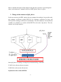
1. Change in the structure of pbl_driver
In the new structure each PBL routine does not compute the tendencies, but provides only
the exchange coefficients (called EXCH_H for exchange coefficient for heat, and
EXCH_M the exchange coefficient for momentum). Then the tendencies for the different
variables are estimated in a routine called DIFF3D at the end of pbl_driver. This new
structure can be represented as.
In the pbl_driver everything is managed by an hardcoded flag, called idiff.
If idiff=1 the code uses the new structure.
If idiff=0 the code uses the old structure.
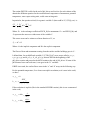
Explanation of the routine DIFF3D.
2 The routine DIFF3D is called at the end of pbl_driver and it solves for each column of the
domain the diffusion equation for the two horizontal components of momentum, potential
temperature, water vapor mixing ratio, could water mixing ratio.
In particular, the equation solved, for a generic variable C (that could be U,V,TH,Q, etc). is:
C 1  
C 

 K H
  Sc
t
z 
 z 
Where K H is the exchange coefficient EXCH_H (for momentum K M and EXCH_M), and
S c represents the sources or sinks terms of the variable C.
This source term can be written as a linear function of C, or:
S c  AC  B
Where A is the implicit component and B is the explicit component.
The fluxes of heat and momentum coming from the surface and the buildings goes in S c .
I defined then, for each diffused variable (U,V,TH,QV,QC), new arrays called a_u, a_v,
a_t, a_q, a_qc, and b_u, b_v, b_t, b_q, b_qc, that are filled at the beginning of the
pbl_driver routine and passed to the diff3d routine at the end of pbl_driver. If some of the
pbl schemes has a non local term, it can goes in the “b” variables.
If BEP is not used, the surface fluxes enter in the “a” and “b” arrays in the following way:
For the potential temperature, if we choose an explicit resolution (as it is now in the code)
we have:
a _ t i ,1, j  0
b _ t i ,1, j 
HFX i , j
 i ,1, j C p z i ,1, j
If the resolution is implicit (like in the standard MYJPBL routine) (this is now commented
in the code)
a _ t i ,1, j  akhsi ,1, j
b _ t i ,1, j  akhsi ,1, j
1
z i ,1, j
thz 0 i , j
z i ,1, j
3 Which is equivalent to write, for the lowest model level (n indicates the time):
S TH 

1
K H  o   n 1
z

For water vapor: explicitely
a _ qi ,1, j  0
QFX i , j
b _ qi ,1, j 
 i ,1, j z i ,1, j
And implicitely
a _ q i ,1, j  akhsi ,1, j
b _ qi ,1, j  akhsi ,1, j
1
z i ,1, j
qz 0 i , j
z i ,1, j
For momentum, the resolution is done implicitly, starting from the consideration that the
momentum flux at the surface for U and V is:
SU  u*
2
SV  u*
2
U
(U  V 2 )
V
2
(U  V 2 )
2
Then taking the U and V at numerator at time n+1 (while those at denominator are kept at
time n) , we have
S U  u *
2
1
U n 1
2
2
(U  V ) z
1
V n 1
S V  u *
2
2
(U  V ) z
2
and
4 a _ u i ,1, j  u*
2
i ,1, j
U
2
i ,1, j
1
 Vi ,21, j z i ,1, j
U
2
i ,1, j
1
 Vi ,21, j z i ,1, j

b _ u i ,1, j  0.
a _ vi ,1, j  u*
2
i ,1, j

b _ vi ,1, j  0.
If BEP is used, those values are weighted average (using the fraction of urban area in the
cell) with the values of a, and b terms coming from the BEP routine.
At the moment, this new structure works with MYJPBL and BOULAC schemes. It is
planned to make it working with any of the PBL schemes.
Numerical details of the routine.
If we discretize the equation
C 1  
C 

 K H
  AC  B
 z 
t
z 
Using the convention that n indexes indicate the time, lowercase “i” indicates the face of
the level, while UPPERCASE I indicates the center of the level, or:
We have:
5 CI
n 1
n
 CI
C  CI
C  C I 1 
1 1 
  AI C In 1  BI
  i 1 K i 1 I 1

 i K i I
t
z i 1
z i 
 I z I 
Since the density  is known at the center, it is interpolated at the faces, as follows:
 I z I 1   I 1 z I
i 
z I  z I 1
Moreover,
z i 
z I  z I 1
2
Then, defining a local variable to simplify the notation as
cddz i   i K i
1
z i
The full equation can be rewritten as:
CI
n 1
 CI
1 1
cddzi 1 C I 1  C I   cddzi C I  C I 1   AI C In1  BI

t
 I z I
n
And re-arranged as
 1 t
1 t
 1 t
cddz i C In11  (1. 
cddz i 1C In11  C In  BI t
(cddz i 1  cddz i )  AI t )C In 1 
 I z I
 I z I
 I z I
This can be solved by inversion of a tridiagonal matrix
 2 I
 1
 I




 3I
 2I
 1I
 3I
 2I
 1I
 3I
 2I
 1I
 C In 1    I 
  n 1    
 C I   I 
  C In 1    I 
 
 
 3 I  C In 1    I 
 2 I  C In 1    I 
Where the lower diagonal is
 1I 
 1 t
cddz i
 I z I
6 The main diagonal
 2 I  1. 
1 t
(cddz i 1  cddz i )  AI t
 I z I
The upper diagonal
 3I 
 1 t
cddz i 1
 I z I
And the right hand side term
 I  C In  BI t
The problem is solved by matrix inversion, using the subroutine “invert”.
If BEP is used, moreover, the air volume of the cell (without buildings), as well as the air
surface at the faces of the grid cell, are taken into account through the introduction of the
two parameters vl and sf, which are the fraction of the volume cell not occupied by
buildings (vl), and the fraction of surface (at the faces of the grid cell), not occupied by
buildings (sf, see eqn. 21 in Martilli et al. 2002).
The equations are then modified as follows:
cddz i  sf i  i K i
 1I 
1
t
cddz i
 I vl I z I
 2 I  1. 
 3I 
1
z i
t
(cddz i 1  cddz i )  AI t
 I vl I z I
1
1
t
cddz i 1
 I vl I z I
The routine computes also diagnostically the vertical turbulent fluxes of momentum
(WU_TUR, WV_TUR,WT_TUR,WQ_TUR). These are 3D variables that are in the outputs
(can be used for analysis of the PBL schemes, for example).
7 2. How to use WRF with BEP (multilayer Urban Canopy Model).
This document explains how to use the multilayer urban canopy model BEP implemented
in the meteorological model WRF.
In a city, the sources/sinks of heat, momentum, and turbulent kinetic energy are not
localized only at the surface, but they are vertically distributed in the whole urban canopy
layer. This is one of the reasons of the differences in the vertical structure of the Surface
Layer between cities and flat rural areas. The inclusion of BEP attempts to simulate this
effect (details about the formulation can be found in Martilli et al. 2002).
In order to get full advantage of the scheme it is necessary to run the model with a very
high vertical resolution (5-10m in the lowest levels), in order to have several numerical
layers within the urban canopy. The drawback of this approach is that the CPU time may
increase. For this reason, it is suggested to use BEP to reproduce past case studies, where
the CPU constraint is less important than for weather forecast. It is also expected that the
impact of BEP will be more relevant for air quality or urban climate studies, where the
behaviour of the atmosphere in the urban canopy is particularly important (because it is
where the people live), rather than for weather forecast studies.
The files to modify to run WRF-BEP are namelist.input, and URBPARM.TBL (see detailed
explanation below). If new urban classes are added, also the landuse file needs to be
modified accordingly. Respect to the single layer UCM, the only extra input needed is the
vertical distribution of building heights for each urban class, which should be included in
URBPARM.TBL (see below). By default, there are no new outputs specific for BEP. The
impact of the scheme will be visible in the 3D temperature and wind fields. The 2m
temperature and 10m winds have been forced equal to the lowest model level This is
mainly for two reasons: a) Monin-Obukhov Similarity Theory is not valid in the urban
canopy, so that it is impossible to derive the 2m and 10m values using the log-law, b) to run
WRF-BEP it is necessary to have a very high vertical resolution (5-10m), so that the
differences between the lowest model level value and the 2m and 10m values are expected
to be small.
1.
How to run WRF with BEP.
namelist.input
To run WRF with BEP, it is necessary to set the option sf_urban_physics=2 in the
namelist.input file. Variable sf_urban_physics is a multidomain variable, so a value should
be set for each domain. Again it is suggested to use BEP only for the inner domains, with
horizontal resolution of the order of few kilometres or less, to save CPU time. We suggest
8 also using the 6th order filter, in order to avoid oscillations that may arise at the border of
the city where a strong change in roughness is present.
At the moment, BEP has been coupled only with the NOAH land surface scheme (so it
works only with sf_surface_physics=2).
Moreover, BEP works with two PBL schemes: MYJ, and BOULAC (Bougeault and
Lacarrere, 1989). This latter has been recently implemented, (option bl_pbl_phyiscs= 8).
Future plans are to couple BEP with YSU.
If the standard USGS classes are used, there is only one urban class (landuse type =1). The
parameters of this class have been set equal to class 2 (Hi density residential) in the
URBPARM.TBL (see below).
Alternatively you can add three extra urban classes, each one characterized by values of the
thermal properties of the materials, and of the urban morphology (see file
URBPARM.TBL).
In namelist.input, the parameter num_urban_layer should be added in the physics section.
This should be equal to, at least, the product of nz_um*ndm*nwr_u, set in
module_sf_bep.F.
If we use the 33 categories mentioned below, num_land_cat must be put equal to 33 in
namelist.input.
URBPARM.TBL
In the file URBPARM.TBL the urban classes are defined. By default, we defined three
classes (Please note that BEP assumes different building heights than UCM, in the standard
table and people should check for their specific urban area if this is suitable).
31: Low Intensity residential: Includes areas with a mixture of constructed materials and
vegetation. Constructed materials account for 30-80 percent of the cover. Vegetation may
account for 20 to 70 percent of the cover. These areas most commonly include singlefamily housing units. Population densities will be lower than in high intensity residential
areas.
32: High Intensity residential: Includes highly developed areas where people reside in
high numbers. Examples include apartment complexes and row houses. Vegetation
accounts for less than 20 percent of the cover. Constructed materials account for 80 to100
percent of the cover.
9 33: Commercial/Industrial/Transportation - Includes infrastructure (e.g. roads, railroads,
etc.) and all highly developed areas not classified as High Intensity Residential.
If you are simulating an US city, you can use the NLCD (2001) which has following 4
urban categories instead of 3 as is the case with 1992 data.
21. Developed, Open Space - Includes areas with a mixture of some constructed materials,
but mostly vegetation in the form of lawn grasses. Impervious surfaces account for less
than 20 percent of total cover. These areas most commonly include large-lot single-family
housing units, parks, golf courses, and vegetation planted in developed settings for
recreation, erosion control, or aesthetic purposes
22. Developed, Low Intensity - Includes areas with a mixture of constructed materials and
vegetation. Impervious surfaces account for 20-49 percent of total cover. These areas most
commonly include single-family housing units.
23. Developed, Medium Intensity - Includes areas with a mixture of constructed materials
and vegetation. Impervious surfaces account for 50-79 percent of the total cover. These
areas most commonly include single-family housing units.
24. Developed, High Intensity - Includes highly developed areas where people reside or
work in high numbers. Examples include apartment complexes, row houses and
commercial/industrial. Impervious surfaces account for 80 to100 percent of the total cover.
The following remapping procedure should be adopted,
The land use categories 21 and 22 should be mapped to land use category 31,
The land use category 23 should be mapped to 32, and
The land use category 24 should be mapped to 33.
The procedure to download the data and the source code to change the data to the
compatible WPS format is described at
http://www.mmm.ucar.edu/people/duda/files/how_to_hires.html
There are 2 sample programs available at this site to process the NLCD (1992) data and the
NLCD (2001) data.
If you are simulating a city not in the US, and you have data to identify the three extra
urban classes, you need to add the extra classes to the landuse file.
For the moment we limited to only three urban categories. It is possible to have more
categories but this will need to introduce some changes in the code. If the user has detailed
10 information on urban morpohology is encouraged to create as many urban classes as he
needs to better represent the city is studying.
The values of thermal properties and urban morphology for each urban class are defined in
URBPARM.TBL. Several variables are common to UCM and BEP, while others are
specific only to BEP. Below is an example of the file, where the variables that are for BEP
or UCM are indicated
# Urban Parameters depending on Urban type
# USGS
Number of urban categories: 3
#
# Where there are multiple columns of values, the values refer, in
# order, to: 1) Commercial, 2) High intensity residential, and 3) Low
# intensity residential: I.e.: UCM, BEP
#
# Index:
1
2
3
# Type: Commercial, Hi-dens Res, Low-dens Res
#
#
# ZR: Roof level (building height) [ m ] UCM
#
ZR: 10.0, 7.5, 5.0
11 #
# ROOF_WIDTH: Roof (i.e., building) width [ m ] UCM
#
(KWM Just made up some numbers for the time being)
#
ROOF_WIDTH: 10.0, 9.4, 8.3
#
# ROAD_WIDTH: road width [ m ] UCM
#
(KWM Just made up some numbers for the time being)
#
ROAD_WIDTH: 10.0, 9.4, 8.3
#
# AH: Anthropogenic heat [ W m{-2} ] UCM
#
AH: 90.0, 50.0, 20.0
#
# FRC_URB: Fraction of the urban landscape which does not have natural
#
vegetation. [ Fraction ] UCM, BEP
#
FRC_URB: 0.95, 0.9, 0.5
12 #
# CAPR: Heat capacity of roof [ J m{-3} K{-1} ] UCM, BEP
#
CAPR: 1.0E6, 1.0E6, 1.0E6,
#
# CAPB: Heat capacity of building wall [ J m{-3} K{-1} ] UCM, BEP
#
CAPB: 1.0E6, 1.0E6, 1.0E6,
#
# CAPG: Heat capacity of ground (road) [ J m{-3} K{-1} ] UCM, BEP
#
CAPG: 1.4E6, 1.4E6, 1.4E6,
#
# AKSR: Thermal conductivity of roof [ J m{-1} s{-1} K{-1} ] UCM, BEP
#
AKSR: 0.67, 0.67, 0.67,
#
13 # AKSB: Thermal conductivity of building wall [ J m{-1} s{-1} K{-1} ] UCM, BEP
#
AKSB: 0.67, 0.67, 0.67,
#
# AKSG: Thermal conductivity of ground (road) [ J m{-1} s{-1} K{-1} ] UCM, BEP
#
AKSG: 0.4004, 0.4004, 0.4004,
#
# ALBR: Surface albedo of roof [ fraction ] UCM, BEP
#
ALBR: 0.20, 0.20, 0.20
#
# ALBB: Surface albedo of building wall [ fraction ] UCM, BEP
#
ALBB: 0.20, 0.20, 0.20
#
# ALBG: Surface albedo of ground (road) [ fraction ] UCM, BEP
#
14 ALBG: 0.20, 0.20, 0.20
#
# EPSR: Surface emissivity of roof [ - ] UCM, BEP
#
EPSR: 0.90, 0.90, 0.90
#
# EPSB: Surface emissivity of building wall [-] UCM, BEP
#
EPSB: 0.90, 0.90, 0.90
#
# EPSG: Surface emissivity of ground (road) [ - ] UCM, BEP
#
EPSG: 0.95, 0.95, 0.95
#
# Z0R: Roughness length for momentum, over roof [ m ] UCM, BEP
#
Z0R: 0.01, 0.01, 0.01
15 #
# Z0B: Roughness length for momentum, over building wall [ m ]
#
Only active for CH_SCHEME == 1 UCM
#
Z0B: 0.01, 0.01, 0.01
#
# Z0G: Roughness length for momentum, over ground (road) [ m ]
#
Only active for CH_SCHEME == 1 UCM, BEP
#
Z0G: 0.01, 0.01, 0.01
#ifdef _FOR_ALBERTO_
STREET PARAMETERS: BEP
# urban
street
street
# category direction
building
width
width
# [index] [deg from N] [m]
[m]
1
0.0
15.0
15.0
1
90.0
15.0
15.0
2
0.0
15.0
15.0
2
90.0
15.0
15.0
16 3
0.0
15.0
15.0
3
90.0
15.0
15.0
END STREET PARAMETERS
BUILDING HEIGHTS: 1
#
height Percentage
#
[m]
[%]
5.0
30.0
10.0
40.0
15.0
30.0
END BUILDING HEIGHTS
BUILDING HEIGHTS: 2
#
height Percentage
#
[m]
[%]
10.0
3.0
15.0
7.0
20.0
12.0
25.0
18.0
30.0
20.0
35.0
18.0
17 40.0
12.0
45.0
7.0
50.0
3.0
END BUILDING HEIGHTS
BUILDING HEIGHTS: 3
#
height Percentage
#
[m]
[%]
5.0
50.0
10.0
50.0
END BUILDING HEIGHTS
#endif
#
# DDZR: Thickness of each roof layer [ m ]
#
This is currently NOT a function urban type, but a function
#
of the number of layers. Number of layers must be 4, for now. UCM
#
DDZR: 0.05, 0.05, 0.05, 0.05
#
# DDZB: Thickness of each building wall layer [ m ]
#
This is currently NOT a function urban type, but a function
#
of the number of layers. Number of layers must be 4, for now. UCM
18 #
DDZB: 0.05, 0.05, 0.05, 0.05
#
# DDZG: Thickness of each ground (road) layer [ m ]
#
This is currently NOT a function urban type, but a function
#
of the number of layers. Number of layers must be 4, for now. UCM
#
DDZG: 0.05, 0.25, 0.50, 0.75
#
# BOUNDR: Lower boundary condition for roof layer temperature [ 1: Zero-Flux, 2: T =
Constant ] UCM
#
BOUNDR: 1
#
# BOUNDB: Lower boundary condition for wall layer temperature [ 1: Zero-Flux, 2: T =
Constant ] UCM
#
BOUNDB: 1
#
19 # BOUNDG: Lower boundary condition for ground (road) layer temperature [ 1: ZeroFlux, 2: T = Constant ] UCM
#
BOUNDG: 1
#
# TRLEND: Lower boundary condition for roof temperature [ K ] UCM
#
TRLEND: 293.00, 293.00, 293.00
#
# TBLEND: Lower boundary temperature for building wall temperature [ K ] UCM
#
TBLEND: 293.00, 293.00, 293.00
#
# TGLEND: Lower boundary temperature for ground (road) temperature [ K ] UCM
#
TGLEND: 293.00, 293.00, 293.00
#
# Ch of Wall and Road [ 1: M-O Similarity Theory, 2: Empirical Form of Narita et al.,
1997 (recommended) ] UCM
20 #
CH_SCHEME: 2
#
# Surface and Layer Temperatures [ 1: 4-layer model, 2: Force-Restore method ] UCM
#
TS_SCHEME: 1
#
# AHOPTION [ 0: No anthropogenic heating, 1: Anthropogenic heating will be added to
sensible heat flux term ] UCM
#
AHOPTION: 0
#
# Anthropogenic Heating diurnal profile. UCM
# Multiplication factor applied to AH (as defined in the table above)
# Hourly values ( 24 of them ), starting at 01 hours Local Time.
# For sub-hourly model time steps, value changes on the hour and is
# held constant until the next hour.
#
#
21 AHDIUPRF: 0.16 0.13 0.08 0.07 0.08 0.26 0.67 0.99 0.89 0.79 0.74 0.73 0.75 0.76 0.82
0.90 1.00 0.95 0.68 0.61 0.53 0.35 0.21 0.18
Users are invited to adapt these values to their case.
Initialization.
The initial temperatures for wall roof and street are initialized in the subroutine:
urban_var_init of the module_sf_urban.F.
The names of the variables are:
TRB_URB4D = roof temperature
TW1_URB4D, and TW2_URB4D= wall temperatures
TGB_URB4D= street temperature.
Note that the values of the initial temperature at the deepest level are kept constant for the
whole simulation.
By default they are initialized with TSLB.
2. Routines modified
The new urban scheme is in routine module_sf_bep.F.
Other routines modified are:
in phys:
module_pbl_driver.F
module_surface_driver.F
module_sf_noahdrv.F
in dyn_em:
module_first_rk_step_part1.F
start_em.F
3. New variables added in Registry
The source/sinks induced by the buildings are written as:
S   A u  B 
22 Where can be an horizontal wind component, the potential temperature, or the moisture.
The new variables added are:
a_u_bep = this is a 3D variable that brings the implicit part of the momentum sink (xcomponent), induced by the buildings ( Au )
b_u_bep = this is a 3D variable that brings the explicit part of the momentum sink (xcomponent), induced by the buildings ( B u )
a_v_bep = this is a 3D variable that brings the implicit part of the momentum sink (ycomponent), induced by the buildings
b_v_bep = this is a 3D variable that brings the explicit part of the momentum sink (ycomponent), induced by the buildings
a_t_bep = this is a 3D variable that brings the implicit part of the potential temperature
source/sink induced by the buildings
b_t_bep = this is a 3D variable that brings the explicit part of the potential temperature
source/sink, induced by the buildings
a_q_bep = this is a 3D variable that brings the implicit part of the moisture source/sink
induced by the buildings
b_q_bep = this is a 3D variable that brings the explicit part of the moisture source/sink,
induced by the buildings
a_e_bep = this is a 3D variable that brings the implicit part of the tke source/sink induced
by the buildings
b_e_bep = this is a 3D variable that brings the explicit part of the tke source/sink, induced
by the buildings
dlg_bep, dl_u_bep are length scales needed to estimate the impact of buildings on tke
sf_bep, vl_bep are the air surface and volume fraction, left by the buildings in the urban
canopy.
References
Bougeault, P. and Lacarrère, P. 1989. Parameterization of orography-induced turbulence
in a mesobeta-scale model. Mon. Wea. Rev. 117: 1872-1890.
23 Martilli, A., Clappier, A., and Rotach, M. W., 2002,’An urban surface exchange
parameterization for mesoscale models’, Boundary-Layer Meteorol., 104, 261-304.
24